ae2-wq-01.pdf
113
January 2009 Environmental Impact Statement for the Lower Churchill Hydroelectric Generation Project Water Quality and Quantity Report 1 of 5 Component Studies Aquatic Environment (2) Water and Sediment Modeling in the Lower Churchill River
-
Upload
angel-maldonado-mendivil -
Category
Documents
-
view
13 -
download
6
Transcript of ae2-wq-01.pdf
January 2009
Environmental Impact Statement for the Lower Churchill Hydroelectric Generation Project
WWaatteerr QQuuaalliittyy aanndd QQuuaannttiittyy
Report 1 of 5
CCoommppoonneenntt SSttuuddiieessAAqquuaattiicc EEnnvviirroonnmmeenntt ((22))
Water and Sediment Modeling in the Lower Churchill River

WATER AND SEDIMENT MODELLING IN THE LOWER CHURCHILL RIVER
ENVIRONMENTAL BASELINE REPORT LCP #535725
FINAL REPORT
August 20, 2008
Prepared by Minaskuat Inc. for
Newfoundland and Labrador Hydro


Lower Churchill Hydroelectric Generation Project
MIN0315.22/1026782 • Water and Sediment Modelling Final EBR • August 20, 2008 Page i © Minaskuat Inc. 2008
EXECUTIVE SUMMARY
As part of its expanded energy mandate, Newfoundland and Labrador Hydro (“Hydro”) proposes to develop the hydroelectric potential of the lower Churchill River, including a 2,000 megawatt (MW) project at Gull Island and a 824 MW project at Muskrat Falls (the “Project”). In 2006, Hydro commissioned an environmental assessment of the Project including this study, which projects nutrient (phosphorus (P)) and total suspended sediment (TSS) levels in the lower Churchill River post-impoundment.
Long term trends in suspended sediment and P in the main stem of the Churchill River system, as a result of the Project, were projected using a simulation model. The lower Churchill River was divided into eight river reaches from Churchill Falls to Happy Valley-Goose Bay, including Lake Winokapau, two reaches in Gull Island reservoir and three in Muskrat Falls reservoir. Average concentrations of TSS and total phosphorus (TP), the limiting nutrient in most water bodies, were modelled in surface water, deep water and bottom sediment cells. The primary sediment and P inputs were shoreline erosion and vegetation decomposition, with minor input from unregulated surface runoff. The model sensitivity to selected key parameters was tested by setting those parameters to high and low values. The best-case and worst-case scenarios were also determined by setting all key sensitivity analysis parameters to values that produced the highest and lowest TSS and TP concentrations. Results were compared against TSS and TP levels from other reservoirs, relevant water bodies and water courses.
Concentrations of both TSS and TP had similar annual cycles post-impoundment, with elevated concentrations during ice-free periods and rapid decreases to near-baseline concentrations during the ice-covered periods, when little shoreline erosion or vegetation decomposition occurred. Overall, the greatest increases in TSS and TP concentrations were observed in reaches downstream of the Gull Island reservoir (i.e., Muskrat Falls reservoir and Happy Valley). These reaches also had the greatest shoreline erosion potential. Concentrations of both variables peaked in the first two years post-impoundment and decreased thereafter. By the end of the 20-year model scenarios, concentrations of both variables in all model cells had reached near-equilibrium levels and beyond this timeframe, yrs 20-50, concentrations approximate current baseline levels. Long-term trends in TSS and TP closely followed the model erosion rate and vegetation decomposition functions as these were the primary sediment and P inputs. When compared to TSS and TP concentrations from other reservoirs and river systems, the model projections had similar general patterns of peaks and recoveries, and intra-annual cycles. The models were most sensitive to variation in the rates of river flow (affecting both TSS and TP), vegetation decomposition (TP only), reservoir clearing (TP only), and sediment settling (TSS only).
Projected peak TSS concentrations ranged from <1 to approximately 30 mg/L in the various modelled river reaches, and occurred during the first year post-impoundment. However, by the end of the 20-year modelling projection, concentrations from all reaches were below 2 mg/L. According to Canadian Council of Ministers of the Environment (CCME) guidelines, long-term increases in TSS should not exceed 5 mg/L above baseline. Applying these guidelines is difficult due to the natural variability of TSS in river systems, and also because the river is undergoing a shift from a river to reservoir. While the projected mean concentrations remain below the maximum concentration reported from the baseline study (127 mg/L), TSS concentrations will be elevated for longer periods of time during the open water season. Projected TP concentrations of the river system rose to between 0.013 and 0.115 mg/L; nutrient inputs to the river post-impoundment will likely raise the trophic status. However, primary production is unlikely to reach maximum potential due to the flow through of impounded river systems and the counteractive shading effect caused by simultaneously increased TSS concentrations.

Lower Churchill Hydroelectric Generation Project
MIN0315.22/1026782 • Water and Sediment Modelling Final EBR • August 20, 2008 Page ii © Minaskuat Inc. 2008
TABLE OF CONTENTS
Page No.
1.0 INTRODUCTION ..................................................................................................................... 1-1
1.1 Lower Churchill Hydroelectric Generation Project ................................................................ 1-1
1.2 Effects of Watercourse Impoundment on Sediment and Phosphorus Dynamics .................. 1-2
1.2.1 Reservoir Erosion .......................................................................................................... 1-2
1.2.2 Trends in Reservoir Phosphorus Concentrations and Primary Production ..................... 1-3
1.2.3 Classification of Trophic State in Lakes and Impoundments .......................................... 1-3
1.2.4 Baseline Water Quality in the Lower Churchill River ...................................................... 1-4
1.3 Report Organization ............................................................................................................. 1-6
2.0 STUDY TEAM ......................................................................................................................... 2-1
3.0 STUDY OBJECTIVES ............................................................................................................. 3-1
4.0 STUDY AREA ......................................................................................................................... 4-1
5.0 MODEL DEVELOPMENT AND ANALYSIS METHODS .......................................................... 5-1
5.1 Mass Balance Modelling Concepts ...................................................................................... 5-1
5.2 The STELLA® Modelling Framework ................................................................................... 5-4
5.3 Mass Flux Between Compartments...................................................................................... 5-4
5.3.1 Surface Compartment to Surface Compartment Mass Flux ........................................... 5-4
5.3.2 Deep Compartment to Deep Compartment Mass Flux .................................................. 5-5
5.3.3 Surface Compartment to Deep Compartment Mass Flux .............................................. 5-6
5.3.4 Water Compartment to Sediment Compartment Mass Flux ........................................... 5-7
5.4 Values Used in the Model .................................................................................................... 5-8
5.4.1 Geographic Information System Measurements ............................................................ 5-8
5.4.2 Surface Compartment Loading .................................................................................... 5-10
5.4.3 Biomass Decomposition Rate Calculations ................................................................. 5-11
5.4.4 Ice-free Season ........................................................................................................... 5-11
5.4.5 Regulated Flow Volumes ............................................................................................ 5-12
5.4.6 Unregulated Flow Volumes ......................................................................................... 5-12
5.4.7 Phosphorus Estimates ................................................................................................ 5-13
5.4.8 Settling Velocities for Silt and Clay .............................................................................. 5-14
5.4.9 Vertical Mixing and Deep Water Dispersion Coefficients ............................................. 5-14
5.5 Model Sensitivity Analysis .................................................................................................. 5-15
5.5.1 Shoreline Erosion Intensity .......................................................................................... 5-16
5.5.2 Baseline Total Suspended Solids Concentration in Water and Silt and Clay Fractions ..................................................................................................................... 5-17
5.5.3 Baseline Phosphorus Concentration in Water ............................................................. 5-18
Lower Churchill Hydroelectric Generation Project
MIN0315.22/1026782 • Water and Sediment Modelling Final EBR • August 20, 2008 Page iii © Minaskuat Inc. 2008
5.5.4 Vertical Mixing (Mixer) and Deep Water Dispersion (Dispers) ..................................... 5-18
5.5.5 Settling Velocities of Silt and Clay ............................................................................... 5-19
5.5.6 Water/Sediment Partition Coefficient (Kd) for Phosphorus ........................................... 5-19
5.5.7 Biomass Decomposition Rate ..................................................................................... 5-20
5.5.8 Annual River Flow ....................................................................................................... 5-21
5.5.9 Reservoir Clearing ...................................................................................................... 5-21
6.0 RESULTS ................................................................................................................................ 6-1
6.1 Pattern of Intra-annual Total Suspended Solids and Total Phosphorus Cycle ...................... 6-1
6.2 Long-term Suspended Sediment Projections ....................................................................... 6-1
6.2.1 Best Estimate Scenario Results .................................................................................... 6-1
6.2.2 Sensitivity Analysis for Total Suspended Solids ............................................................ 6-6
6.3 Long-term Phosphorus Projections ...................................................................................... 6-7
6.3.1 Best Estimate Scenario Results .................................................................................... 6-7
6.3.2 Sensitivity Analysis of Total Phosphorus ....................................................................... 6-9
7.0 DISCUSSION .......................................................................................................................... 7-1
7.1 Projected Total Suspended Sediment Concentrations ......................................................... 7-1
7.2 Projected Total Phosphorus Concentrations ........................................................................ 7-2
7.3 Model Sensitivity Analysis .................................................................................................... 7-2
7.4 Model Uncertainties ............................................................................................................. 7-3
7.4.1 Erosion rates ................................................................................................................. 7-3
7.4.2 Spatial Sediment Distribution ........................................................................................ 7-4
7.5 Summary and Conclusions .................................................................................................. 7-4
8.0 CLOSURE ............................................................................................................................... 8-1
9.0 REFERENCES ........................................................................................................................ 9-1
9.1 Literature Cited .................................................................................................................... 9-1
9.2 Internet Sites ........................................................................................................................ 9-4
10.0 ACRONYM LIST ................................................................................................................... 10-1

Lower Churchill Hydroelectric Generation Project
MIN0315.22/1026782 • Water and Sediment Modelling Final EBR • August 20, 2008 Page iv © Minaskuat Inc. 2008
LIST OF TABLES
Page No.
Table 1-1 Canadian Council of Ministers of the Environment Environmental Quality Guideline Trophic Categories for Lakes ........................................................................ 1-4
Table 1-2 Report Organization ..................................................................................................... 1-7
Table 2-1 Study Team for Total Suspended Solids and Phosphorus Modeling Study .................. 2-1
Table 5-1 Data Generated by GIS Catchment Areas Including Phosphorus, Silt and Clay Loadings ...................................................................................................................... 5-9
Table 5-2 Monthly Mean Flow Rates at Gauging Station EC 03OD005 ...................................... 5-12
Table 5-3 Monthly Mean Unregulated Runoff Rate for the Lower Churchill River ....................... 5-13
Table 5-4 Minimum, Best Estimate, and Maximum Parameter Values for Model Sensitivity Analysis ...................................................................................................................... 5-16
Table 5-5 Review of Published Phosphorus Kd Values ............................................................... 5-20
Table 6-1 Peak Total Suspended Solids Concentration (mg/L) in Each River Reach ................... 6-6
Table 6-2 Effect on Total Suspended Solids of Adjusting Sensitivity Analysis Parameters from Best-Case to Worst-Case ..................................................................................... 6-7
Table 6-3 Peak Total Phosphorus Concentrations in All River Reaches ....................................... 6-9
Table 6-4 Effect on Total Phosphorus of Adjusting Sensitivity Analysis Parameters from Best-Case to Worst-case............................................................................................ 6-10
LIST OF FIGURES
Page No.
Figure 1-1 Baseline TP Concentrations (mg/L), April 2006 to March 2007 .................................... 1-5
Figure 4-1 Modelled Study Area .................................................................................................... 4-1
Figure 5-1 Conceptual Model of the Lower Churchill River Showing Channel Profile and STELLA® Model Stocks and Flow Icons ...................................................................... 5-2
Figure 6-1 Modelled Total Suspended Solids Concentrations in the Churchill River for Second Year Post-Impoundment .................................................................................. 6-2
Figure 6-2 Modelled Total Phosphorus Concentrations in the Churchill River for Second Year Post-Impoundment .............................................................................................. 6-3
Figure 6-3 Modelled Total Suspended Solids Concentrations in the Churchill River ...................... 6-4
Figure 6-4 Annual Shoreline Erosion Intensity Over Time ............................................................. 6-5
Figure 6-5 Modelled Total Phophorus Concentrations in the Churchill River ................................. 6-8
Figure 6-6 Percent Flooded Biomass Remaining in the Reservoir Over Time ............................... 6-9
LIST OF APPENDICES
Appendix A The STELLA® Model Equations


Lower Churchill Hydroelectric Generation Project
MIN0315.22/1026782 • Water and Sediment Modelling Final EBR • August 20, 2008 Page 1-1 © Minaskuat Inc. 2008
1.0 INTRODUCTION
This model of total suspended sediment (TSS) and nutrients (phosphorus (P)) in the river and proposed reservoirs, was developed and implemented as part of the environmental assessment process for the proposed Lower Churchill Hydroelectric Generation Project (the “Project”), being considered by Newfoundland and Labrador Hydro (“Hydro”). The information provided in this document is intended to support the environmental effects analysis of the Project.
1.1 Lower Churchill Hydroelectric Generation Project
The Project will include hydroelectric generating facilities at Gull Island and Muskrat Falls, and interconnecting transmission lines to the existing Labrador grid. The Gull Island facility will consist of a generating station with a capacity of approximately 2,000 megawatt (MW) and include:
• a dam 99 m high and 1,315 m long and
• a 200 km² reservoir at an assumed full supply level of 125 m above sea level (asl)
The dam will be a central till-cored, rock-fill, zone embankment. The reservoir will be 225 km long, and the area of inundated land will be 85 km² at full supply level. The powerhouse will contain four to six Francis turbines.
The Muskrat Falls facility will consist of a generating station that will be approximately 800 MW in capacity and will include:
• a concrete dam with two sections on the north and south abutments of the river and
• a 107 km² reservoir at an assumed full supply level of 39 m asl
The north section dam will be 32 m high and 180 m long, while the south section will be 29 m high and 370 m long. The north section will serve as a spillway in extreme precipitation events. The reservoir will be 60 km long and the area of inundated land will be 41 km² at full supply level. The powerhouse will contain four to five propeller or Kaplan turbines, or a combination of both.
The interconnecting transmission lines will consist of:
• a 735 kilovolt (kV) transmission line between Gull Island and Churchill Falls and
• two 230 kV transmission lines between Muskrat Falls and Gull Island
The 735 kV transmission line will be 203 km long and the 230 kV transmission lines will be 60 km long. Both lines will likely be lattice-type steel structures. The location of the transmission lines will be north of the Churchill River; the final route is the subject of a route selection study that will be included in the environmental assessment. The lines between Muskrat Falls and Gull Island may be on separate towers, or combined on double-circuit structures.
The Project design may be refined as engineering details become available.
Lower Churchill Hydroelectric Generation Project
MIN0315.22/1026782 • Water and Sediment Modelling Final EBR • August 20, 2008 Page 1-2 © Minaskuat Inc. 2008
1.2 Effects of Watercourse Impoundment on Sediment and Phosphorus Dynamics
1.2.1 Reservoir Erosion
Damming of watercourses for the purpose of generating electricity alters the natural hydrological cycle of the watercourse. In order to provide a relatively stable rate of electricity production, reservoirs are typically created and water regulated according to the seasonal spring freshet and lower winter input. Raising water levels as a result of reservoir creation causes a shift in the shoreline level of the watercourse. As the shoreline is raised from an equilibrium state of erosion, which is dependent on the local topography and stream hydrology, the resulting new reservoir shoreline will be in a state of disequilibrium, and new erosion will occur.
Shorelines in a state of disequilibrium may experience from erosion or slope failure. Types of slope failures are presented in the Bank Stability Study Report (AMEC 2007), and will not be discussed here in detail. The rate of shoreline erosion in an open water body, such as a reservoir, is dependent on the onshore wave energy (a function of wind velocity and fetch distance), the resistance (composition) of the shoreline materials to the erosion process, and the configuration of the shoreline and offshore zone (Newbury and McCullough 1984). The shoreline will change its initial configuration after reservoir filling to a wave-cut bank with growing offshore deposits. In reservoirs, the effect of drawdown during low flow periods has also been shown to be positively related to shoreline erosion and the duration of shoreline instability (Saint-Laurent et al. 2001). Hydroelectric facilities that function closer to run-of-reservoir production rates tend to have less severe erosion events and shorter periods of instability compared to facilities that depend to a higher degree on reservoir drawdown during periods of lower flow.
In Precambrian Shield terrain, the disequilibrium erosion period is dependent on the erosion rate and type of erosion materials, but typically continues until an equilibrium profile is established or until the overburden is removed and the underlying bedrock is reached (Newbury and McCullough 1984). Erosion of shorelines results in sediment inputs into the reservoir. Larger sediment particles (e.g., sand, gravel) deposit quickly and contribute to changing of the offshore zone (Elçi et al. 2007). Smaller particles (e.g., silt and clay) settle at much slower rates, and effectively become suspended in the water column for a period of time dependent on particle size and water turbulence (Kerr 1995, Newbury and McCullough 1984).
In river systems, the period of spring runoff (spring freshet) typically also results in increased concentrations of suspended sediments. Material is carried from terrestrial habitats and the peak flow rates associated with spring freshet cause scouring of deposited sediments. Concentrations of TSS, therefore, typically increase during the spring freshet, or during other spate events, but decline rapidly thereafter as water levels recede.
Relative water levels and flow rates in reservoirs do not increase to the same degree during the spring freshet as in rivers. While sediment from unregulated runoff may increase in the springtime, the most important source of sediment is shoreline erosion as a result of wind-driven wave action during the ice-free period. Concentrations of TSS, therefore, are often elevated during the entire ice-free period and are dependent on summer wind velocity.
Lower Churchill Hydroelectric Generation Project
MIN0315.22/1026782 • Water and Sediment Modelling Final EBR • August 20, 2008 Page 1-3 © Minaskuat Inc. 2008
1.2.2 Trends in Reservoir Phosphorus Concentrations and Primary Production
Impounding river systems causes change to ecosystem productivity and community composition (Hall et al. 1999). While external nutrient loads are unlikely to change, temporal patterns of reservoir production result from changes in nutrient biogeochemistry due to flooding of terrestrial habitat. Sources of nutrients include erosion of newly formed shoreline, leaching of soluble nutrients from flooded soil, and decomposition of inundated vegetation (Kennedy and Walker 1990). In aquatic systems, the nutrient most commonly limiting primary production is P. Nitrogen is frequently limiting in terrestrial systems; however, due to the ability of certain algae and other micro-organisms to fix atmospheric nitrogen, this nutrient can be increased in the system to match the input of P. Therefore, this study focuses on P as the limiting nutrient in the lower Churchill River. While dissolved P (P not adsorbed to suspended particles or sediments) is the biologically available fraction of the total phosphorus (TP), P cycling in dilute and nutrient-limited systems is typically very rapid. Therefore, due to the prevalence of TP reported in the literature, P concentrations in the water are presented as TP in this report, however, in processes related to the release or loading, phosphorus is referred to as P.
A concern following impoundment of watercourses is the potential change in nutrient loading and resulting eutrophication of the reservoir. This phenomenon has been extensively documented in the literature (Kennedy and Walker 1990; Kimmel et al. 1990; Hall et al. 1999; Stockner et al. 2000; Jeppesen et al. 2005). However, the magnitude of eutrophication and extent of its duration are important considerations when examining the long-term effects of impoundment on the productivity of the system, and possible secondary effects on fish populations and communities. Furthermore, it is important to consider the initial trophic status of the system prior to impoundment.
Kimmel et al. (1990) also indicated that productivity of reservoirs may increase for a period of 5 to 20 years post-impoundment. The length of this period depends on the amount of flooded biomass, the magnitude of water level changes, and other factors including water retention time (flushing rate). This period is typically followed by a 3 to 30 year period of reduced production, then a possible gradual increase in fish production (Lindström 1973, in Hall et al. 1999). This is contradicted by Stockner et al. (2000), who indicated that the post-impoundment equilibrium TP concentration in the water column can actually be lower than concentrations pre-impoundment. This is the result of increased sedimentation and losses from discharge, and also to water level fluctuations from drawdown during periods of low water input and high energy demands. One factor relevant to the postulated equilibrium state of reduced production is that many reservoirs discharge water from the hypolimnion, which may be enriched in TP (due to P release from decomposing organic matter as it sinks, or from sediments to the overlying water under anoxic conditions) and is the reverse of what would normally occur in a lake system.
1.2.3 Classification of Trophic State in Lakes and Impoundments
Changes in TP concentrations within reservoirs cause a trophic shift, with an increase in the availability of nutrients immediately following impoundment, and a return to equilibrium conditions similar to pre-impoundment conditions approximately 10 to 20 years later. According to the Canadian Council of Ministers of the Environment (CCME 2004) Trophic Categories for Lakes and Rivers in Canada, the magnitude of the increase in TP post-impoundment will determine the extent to which the affected system will undergo eutrophication (Table 1-1). After the initial increase in TP concentrations, lakes and
Lower Churchill Hydroelectric Generation Project
MIN0315.22/1026782 • Water and Sediment Modelling Final EBR • August 20, 2008 Page 1-4 © Minaskuat Inc. 2008
reservoirs typically return to a trophic state similar to pre-impoundment (Stockner et al. 2000; Jeppesen et al. 2005).
Table 1-1 Canadian Council of Ministers of the Environment Environmental Quality Guideline Trophic Categories for Lakes
TP Concentration (mg/L) Trophic Status
0 to 0.004 Ultra-oligotrophic 0.004 to 0.01 Oligotrophic 0.01 to 0.02 Mesotrophic 0.02 to 0.035 Meso-eutrophic 0.035 to 0.1 Eutrophic >0.1 Hyper-eutrophic Source: CCME 2004.
1.2.4 Baseline Water Quality in the Lower Churchill River
Water quality of the lower Churchill River was assessed in 1998 and again in 2006/07 using similar sampling and analytical techniques and sampling sites (JWEL 1999; Minaskuat Limited Partnership (Minaskuat) 2007a). The survey area was the Churchill River from below Churchill Falls Generating Station downstream to the mouth of the river; areas were identical in both studies. The number of sampling stations was reduced in the 2006/07 study to a subset of the prior study. Ten stations were selected to represent sections of the river. The number of water sampling campaigns was increased from four in 1998 to 15 (i.e., monthly for a year and weekly during spring break-up in 2006). The measured parameters were the same in both studies, although lower reportable levels of detection (RDLs) in 2006/07 provided more information on many parameters that are present at trace levels. The single sediment sampling campaign was similar to that conducted in 1998. While the sampling was conducted by boat in 1998, a helicopter equipped with floats was used in 2006/07. This allowed for timely sampling along the entire river and, with minor exceptions, all stations could be accessed safely in ice-covered and open water conditions.
One additional procedure in the 2006/07 study was the deployment of a series of 14 recording thermistors suspended from anchored buoys at both ends of Lake Winokapau. Although one of the arrays was lost, the other provided a record of water temperatures through the top 25 m of the lake from July through November, 2006.
The water quality in the survey area changed very little between the 1998 and 2006/07 studies. In 1998, concentrations of TP and orthophosphate were typically below RDLs and the Churchill River was identified as being highly oligotrophic (nutrient-poor) system. In 2006/07, nitrogen concentrations typically reflected a similar situation to 1998, with nitrogen compounds below or only slightly above detection limits. However, for TP the 2006/07 laboratory analysis was undertaken using more precise techniques resulting in a lower RDL.
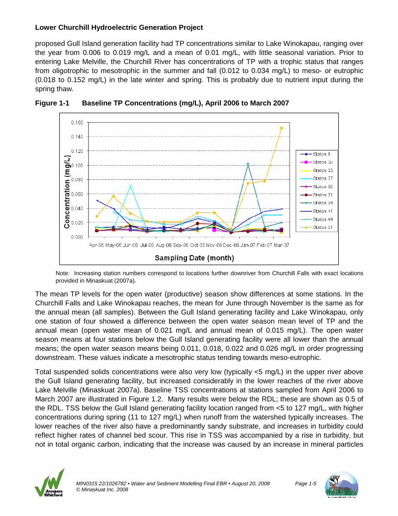
TP in the Churchill River varies along the length of the river and by season (Minaskuat 2007a). Baseline TP concentrations at stations sampled from April 2006 to March 2007 are illustrated in Figure 1.1. TP concentrations below the confluence with Metchin River ranged over the year from 0.006 to 0.016 mg/L, with a mean of 0.012 mg/L and little seasonal variation. Data from Lake Winokapau indicate a generally oligotrophic state, with TP concentrations ranging from 0.006 to 0.012 mg/L and a mean of 0.009 mg/L (i.e., mean of all samples). The river reach between Lake Winokapau and the
Lower Churchill Hydroelectric Generation Project
MIN0315.22/1026782 • Water and Sediment Modelling Final EBR • August 20, 2008 Page 1-5 © Minaskuat Inc. 2008
proposed Gull Island generation facility had TP concentrations similar to Lake Winokapau, ranging over the year from 0.006 to 0.019 mg/L and a mean of 0.01 mg/L, with little seasonal variation. Prior to entering Lake Melville, the Churchill River has concentrations of TP with a trophic status that ranges from oligotrophic to mesotrophic in the summer and fall (0.012 to 0.034 mg/L) to meso- or eutrophic (0.018 to 0.152 mg/L) in the late winter and spring. This is probably due to nutrient input during the spring thaw.
Figure 1-1 Baseline TP Concentrations (mg/L), April 2006 to March 2007
Note: Increasing station numbers correspond to locations further downriver from Churchill Falls with exact locations provided in Minaskuat (2007a).
The mean TP levels for the open water (productive) season show differences at some stations. In the Churchill Falls and Lake Winokapau reaches, the mean for June through November is the same as for the annual mean (all samples). Between the Gull Island generating facility and Lake Winokapau, only one station of four showed a difference between the open water season mean level of TP and the annual mean (open water mean of 0.021 mg/L and annual mean of 0.015 mg/L). The open water season means at four stations below the Gull Island generating facility were all lower than the annual means; the open water season means being 0.011, 0.018, 0.022 and 0.026 mg/L in order progressing downstream. These values indicate a mesotrophic status tending towards meso-eutrophic.
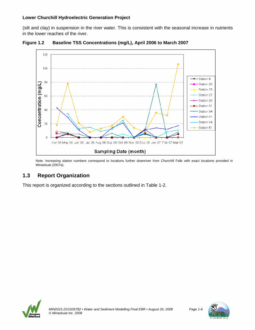
Total suspended solids concentrations were also very low (typically <5 mg/L) in the upper river above the Gull Island generating facility, but increased considerably in the lower reaches of the river above Lake Melville (Minaskuat 2007a). Baseline TSS concentrations at stations sampled from April 2006 to March 2007 are illustrated in Figure 1.2. Many results were below the RDL; these are shown as 0.5 of the RDL. TSS below the Gull Island generating facility location ranged from <5 to 127 mg/L, with higher concentrations during spring (11 to 127 mg/L) when runoff from the watershed typically increases. The lower reaches of the river also have a predominantly sandy substrate, and increases in turbidity could reflect higher rates of channel bed scour. This rise in TSS was accompanied by a rise in turbidity, but not in total organic carbon, indicating that the increase was caused by an increase in mineral particles
Lower Churchill Hydroelectric Generation Project
MIN0315.22/1026782 • Water and Sediment Modelling Final EBR • August 20, 2008 Page 1-6 © Minaskuat Inc. 2008
(silt and clay) in suspension in the river water. This is consistent with the seasonal increase in nutrients in the lower reaches of the river.
Figure 1.2 Baseline TSS Concentrations (mg/L), April 2006 to March 2007
Note: Increasing station numbers correspond to locations further downriver from Churchill Falls with exact locations provided in Minaskuat (2007a).
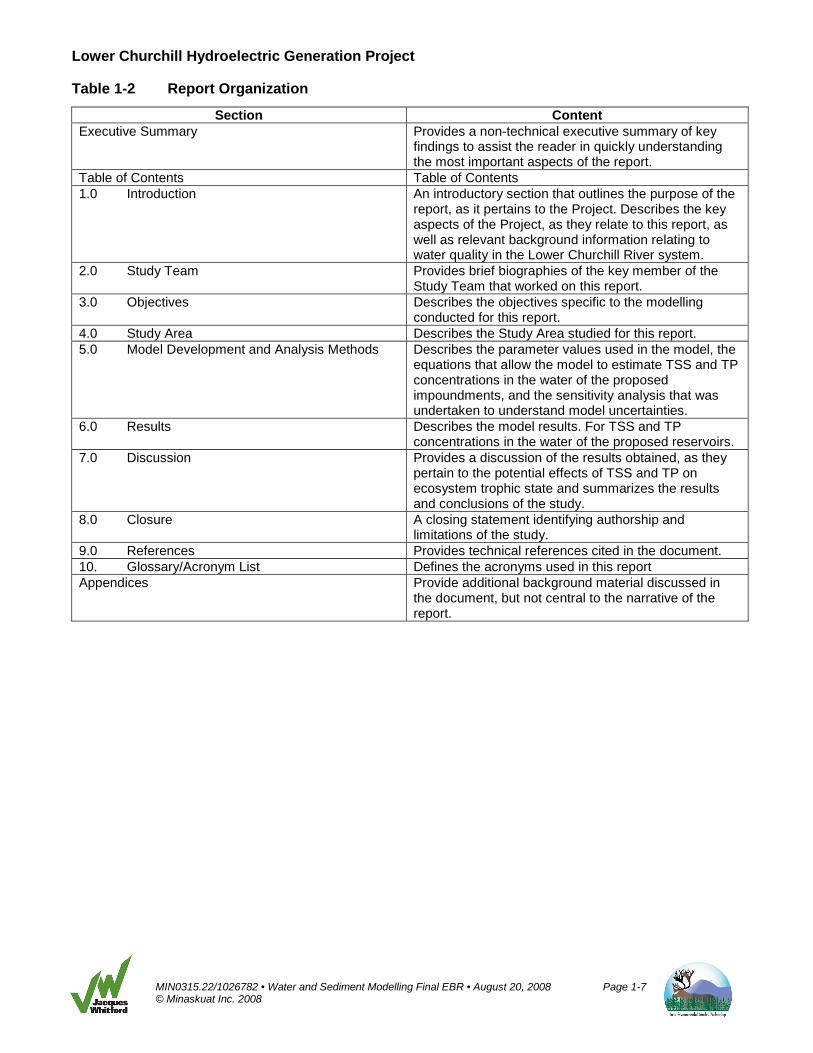
1.3 Report Organization
This report is organized according to the sections outlined in Table 1-2.
Lower Churchill Hydroelectric Generation Project
MIN0315.22/1026782 • Water and Sediment Modelling Final EBR • August 20, 2008 Page 1-7 © Minaskuat Inc. 2008
Table 1-2 Report Organization
Section Content Executive Summary Provides a non-technical executive summary of key
findings to assist the reader in quickly understanding the most important aspects of the report.
Table of Contents Table of Contents 1.0 Introduction An introductory section that outlines the purpose of the
report, as it pertains to the Project. Describes the key aspects of the Project, as they relate to this report, as well as relevant background information relating to water quality in the Lower Churchill River system.
2.0 Study Team Provides brief biographies of the key member of the Study Team that worked on this report.
3.0 Objectives Describes the objectives specific to the modelling conducted for this report.
4.0 Study Area Describes the Study Area studied for this report. 5.0 Model Development and Analysis Methods Describes the parameter values used in the model, the
equations that allow the model to estimate TSS and TP concentrations in the water of the proposed impoundments, and the sensitivity analysis that was undertaken to understand model uncertainties.
6.0 Results Describes the model results. For TSS and TP concentrations in the water of the proposed reservoirs.
7.0 Discussion Provides a discussion of the results obtained, as they pertain to the potential effects of TSS and TP on ecosystem trophic state and summarizes the results and conclusions of the study.
8.0 Closure A closing statement identifying authorship and limitations of the study.
9.0 References Provides technical references cited in the document. 10. Glossary/Acronym List Defines the acronyms used in this report Appendices Provide additional background material discussed in
the document, but not central to the narrative of the report.

Lower Churchill Hydroelectric Generation Project
MIN0315.22/1026782 • Water and Sediment Modelling Final EBR • August 20, 2008 Page 2-1 © Minaskuat Inc. 2008
2.0 STUDY TEAM
The Water and Sediment Modelling in the Lower Churchill River was conducted by Minaskuat. The Study Team included project and study managers, senior and junior researchers (Table 2-1). All team members have in-depth knowledge and experience in their fields of expertise and a broad general knowledge of the work conducted by other specialists in related fields. Brief biographical statements, highlighting project roles and responsibilities and relevant education and employment experience, are provided below.
Table 2-1 Study Team for Total Suspended Solids and Phosphorus Modeling Study
Role Personnel Project Manager Dr. Malcolm Stephenson Researchers/Modellers Dr. Jean-Michel DeVink
Paul Mazzocco Dr. Jay Walmsley
Data management and Reporting Dr. Malcolm Stephenson Dr. Jean-Michel DeVink Kevin Keys Chad Amirault
Malcolm Stephenson, Ph.D., is a Principal and Senior Aquatic Scientist with Jacques Whitford in Fredericton, New Brunswick. He has a background in fisheries and wildlife biology, supplemented by broad post-graduate training in aquatic science and toxicology. Dr. Stephenson is the Scientific Authority for this water quality (TSS and TP) modelling study. His primary areas of specialization are environmental impact assessment and risk assessment, emphasizing multi-disciplinary linkages to environmental restoration, hydrology, ecological modelling, ecotoxicology, geochemistry and applied aquatic ecology. Dr. Stephenson has developed water and sediment quality models for a wide variety of applications, including Precambrian Shield lakes for the Canadian Nuclear Fuel Waste Management Program, the Great Lakes and the Ottawa River for Atomic Energy of Canada Limited, the Sydney Tar Ponds and Sydney Harbour in Nova Scotia to support the Sydney Tar Ponds cleanup efforts, and St. John’s Harbour in Newfoundland and Labrador for Public Works and Government Services Canada.
Jean-Michel DeVink, Ph.D., is an Environmental Scientist at with Jacques Whitford in Fredericton, New Brunswick. His role is primarily in the area of environmental risk assessment. He completed his B.Sc. (2002) in Forestry and Environmental Management at the University of New Brunswick and Ph.D. (2007) in Biology and Ecotoxicology at the University of Saskatchewan. Since 1999, his research and work experiences have focused on wildlife biology as well as landscape level effects of habitat loss and contamination on habitat quality and wildlife populations. His research has taken place in marine, boreal, arctic, and prairie environments in addition to captive experimental settings. Dr. DeVink’s strengths lie in experimental design, ecotoxicology, biostatistical analysis, and habitat assessment.
Paul Mazzocco, B.Sc., is an associate hydrogeologist with over ten years experience with Jacques Whitford. He has experience relating to the identification, assessment, and remediation of hydrocarbons, PCB’s, PAH’s and other contaminants. He has designed and implemented various databases in the assistance of numerous Phase II/III site assessments on residential, commercial and industrial sites. These have included groundwater, soil, air quality and hazardous material studies, recommendations for remedial options, and qualitative/quantitative human health and ecological risk assessments. Mr. Mazzocco’s current focus is in the development and implementation of technology

Lower Churchill Hydroelectric Generation Project
MIN0315.22/1026782 • Water and Sediment Modelling Final EBR • August 20, 2008 Page 2-2 © Minaskuat Inc. 2008
and its assistance towards automated historical data collection, statistical analysis, enhanced data management and analyses including the design, implementation and use of database, GIS, mathematical models and custom Visual Basic programs.
Kevin Keys, M.Sc.F., R.P.F., is a forest ecologist and soil scientist with Jacques Whitford in Dartmouth, Nova Scotia. His primary areas of specialization are ecosystem classification, soil classification, and related management interpretations. Mr. Keys has over 15 years experience working throughout Maritime Canada, British Columbia, and Labrador. He is the author of Forest Soil Types of Nova Scotia: Identification, Description, and Interpretation, and was a leading contributor in the development of Nova Scotia’s forest ecosystem classification system.
Chad Amirault is a GIS cartographer and the Service Director for GIS and Data Management with Jacques Whitford. His responsibilities include GIS business development, strategy and team development. He has extensive experience in database design/management, GIS analysis, cartography, map production, 3-D/environmental modelling and graphic design. Mr. Amirault has been with Jacques Whitford for over four years and has been working with GIS software for over six years. He has worked on many large projects including the Phase II/III Muggah Creek Environmental Assessment and Blue Atlantic Transmission System. Mr. Amirault has developed many in-house cartographic tools as well as initiated the use of new 3-D visualization software. Mr. Amirault received his Diploma in Digital Cartography from the College of Geographic Sciences (COGS), Lawrencetown, Nova Scotia. There, he received intense training in the fields of cartography, GIS and graphic design. In 2000, Mr. Amirault was awarded the CCA President’s Prize for best colour map. In 2001, he received first place at the ESRI users conference map gallery, Dartmouth, Nova Scotia. In 2003, he received second place at the same ESRI users conference. Mr. Amirault is currently a member of the Canadian Cartographic Association the Geomatics Association of Nova Scotia and the Geomatics Industry of Canada.
Lower Churchill Hydroelectric Generation Project
MIN0315.22/1026782 • Water and Sediment Modelling Final EBR • August 20, 2008 Page 3-1 © Minaskuat Inc. 2008
3.0 STUDY OBJECTIVES
The objective of this study was to develop a water and sediment quality model for the lower Churchill River (i.e., that portion of the Churchill River system in Labrador that lies between the tailrace of the existing Smallwood Reservoir, and the mouth of the river entering Lake Melville near Happy Valley-Goose Bay, Labrador) post-impoundment, and to implement the model using the STELLA® modelling software system, to provide estimates of TSS and TP concentrations in the water for a 20-year period post-impoundment.
Specifically, the tasks of this study were to:
• develop a physical model (i.e., segmentation and characterization) of the post-impoundment lower Churchill River, as the framework on which the various water quality models will operate
• include in the model the physical, chemical and biological processes necessary to describe the behaviour of TSS and TP within the impoundments
• run the water quality models to estimate future water quality characteristics and trends in the various reaches until a level of stability is achieved (nominally 20 years) and
• prepare a report documenting the models and the model outputs
The objective of this study was to estimate TSS and TP concentrations for 50 years post-impoundment. However, as it was determined that the processes (shoreline erosion and biomass decomposition) resulting from impoundment that largely determine concentrations of TSS and TP in the Gull Island and Muskrat Falls reservoirs subside within the first 15 years post-impoundment (e.g., Figures 6-4 and 6-6), the model was set to a 20-year time interval. This reduced time interval allows the model to use shorter time steps (dT = 0.25 days), which produced more accurate results during the first 20-year period when the greatest changes occur. Beyond 20 years (20 to 50 years), concentrations of TSS and TP are extrapolated from the 20-year model results and discussed.
Hydro identified three potential scenarios for harvesting of timber and clearing of vegetation in portions of the Churchill River valley to be flooded by the Project that would affect estimates of TP in the two modelled reservoirs. These three scenarios are: a default No Clearing scenario, a Partial Clearing scenario, and a Full Clearing scenario. These scenarios are presented in sub-section 5.5.9.

Lower Churchill Hydroelectric Generation Project
MIN0315.22/1026782 • Water and Sediment Modelling Final EBR • August 20, 2008 Page 4-1 © Minaskuat Inc. 2008
4.0 STUDY AREA
The Project will consist of two hydroelectric generating facilities, located at Gull Island and Muskrat Falls, and an interconnecting electrical transmission line to the existing Labrador grid. The Gull Island generating facility will consist of a large generating facility and reservoir system, while the Muskrat Falls generating facility will have a smaller generating facility and reservoir with run of river generating capacity. The location of the Project and generating facilities is presented in Figure 4-1.
The Study Area comprised the main stem of the lower Churchill River from the Tailrace at Churchill Falls to the mouth of the river where it enters Lake Melville.
Figure 4-1 Modelled Study Area
Lower Churchill Hydroelectric Generation Project
MIN0315.22/1026782 • Water and Sediment Modelling Final EBR • August 20, 2008 Page 5-1 © Minaskuat Inc. 2008
5.0 MODEL DEVELOPMENT AND ANALYSIS METHODS
The STELLA® Version 8.0 modelling software system was used to develop a water quality model for TSS and TP for the proposed Project. A detailed description of the model equations, parameters and documentation is found in Appendix A. The following sections explain the mathematical relationships that were used to estimate concentrations of TSS and TP in the surface water compartments.
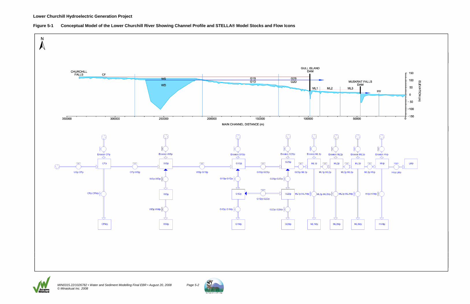
The basic structure of the water quality model is illustrated in Figure 5-1. The physical structure of the river is represented as a series of completely mixed reactors that receive inputs of TSS and TP, and that can exchange water and materials (TSS and TP) with adjacent compartments (i.e., compartments located downstream or beneath). Most of the compartments represent the full water depth, except for those located in the Gull Island reservoir, which are treated as surface (0 to 25 m depth) and deep (>25 m depth) units. This type of model is often referred to as a “cells in series” model, and this approach is commonly used to simulate rivers and estuaries.
The model consists of three “decks”, representing silt, clay, and TP in the water of the lower Churchill River, respectively. Each deck has essentially the same structure, and the silt and clay decks combined represent the TSS.
Within each compartment in each deck, mass balance is observed, so that the mass of silt, clay or TP in any compartment at any time is a direct function of the inputs to and outputs from that compartment. The compartment inputs for TSS typically include the baseline TSS concentration coming from upriver or tributaries (estimated to be 1 mg/L), as well as the mass of silt or clay eroded from the shorelines within each time step of the simulation. For TP, inputs include the baseline TP concentration coming from upriver or tributaries, as well as P released from soils by erosion, and P released from decaying organic matter and vegetation remaining after shoreline clearing. The compartment outputs for TSS and TP typically include losses to deep water compartments or sediments, and down-river transport with hydraulic flushing.
The following sections provide a technical description of the model that was developed and used to estimate TSS and TP concentrations in the lower Churchill River, post-impoundment. The model was implemented using the commercially available modelling software, STELLA®, version 8.1.1 for Windows (see Systems 2004).
5.1 Mass Balance Modelling Concepts
No single model is appropriate for all purposes, and a range of models is often required. Because biological, chemical, geological and physical processes can all affect the transport, dispersion and fate of contaminants, the quantification of the important processes in a given river environment frequently requires multidisciplinary study. However, such studies are often either too costly, or of insufficient duration, resolution and breadth to adequately characterize the receiving system. Thus, other approaches are required.
The mathematical modelling approach can be used to understand and trace the fate and transport of contaminants through a system. A model can be a useful tool for extending limited data sets to predictions of future conditions. However, it should be remembered that a model is an idealized and simplified representation of the environment. Although not a perfect representation, a model can still be useful if it is designed to embody the important features and processes of the original system.
Lower Churchill Hydroelectric Generation Project
MIN0315.22/1026782 • Water and Sediment Modelling Final EBR • August 20, 2008 Page 5-2 © Minaskuat Inc. 2008
Figure 5-1 Conceptual Model of the Lower Churchill River Showing Channel Profile and STELLA® Model Stocks and Flow Icons

Lower Churchill Hydroelectric Generation Project
MIN0315.22/1026782 • Water and Sediment Modelling Final EBR • August 20, 2008 Page 5-3 © Minaskuat Inc. 2008
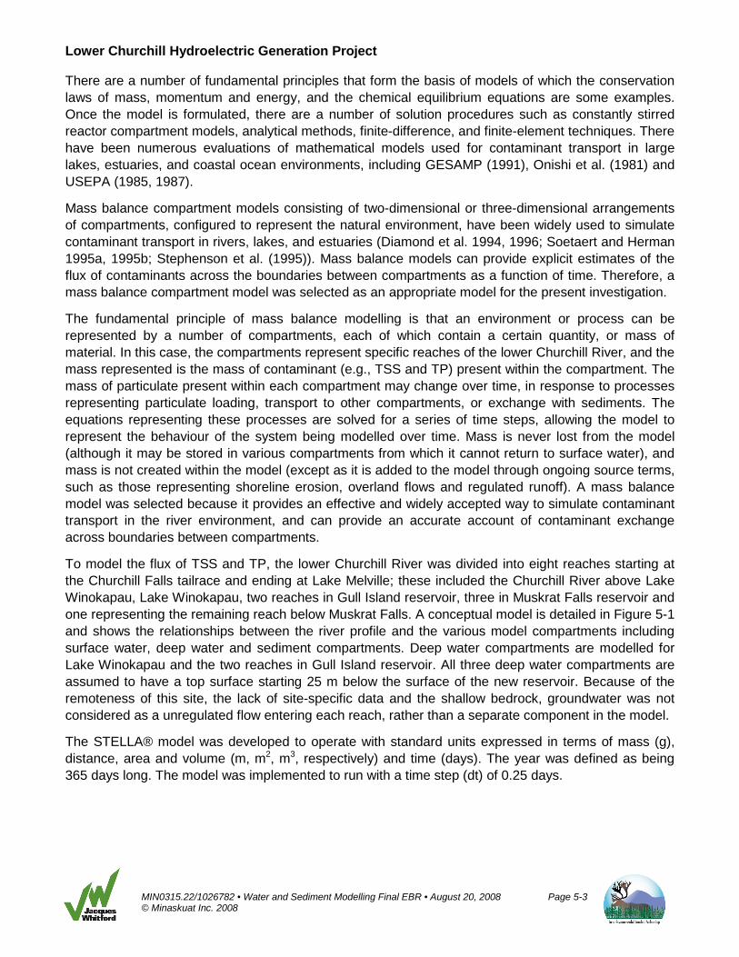
There are a number of fundamental principles that form the basis of models of which the conservation laws of mass, momentum and energy, and the chemical equilibrium equations are some examples. Once the model is formulated, there are a number of solution procedures such as constantly stirred reactor compartment models, analytical methods, finite-difference, and finite-element techniques. There have been numerous evaluations of mathematical models used for contaminant transport in large lakes, estuaries, and coastal ocean environments, including GESAMP (1991), Onishi et al. (1981) and USEPA (1985, 1987).
Mass balance compartment models consisting of two-dimensional or three-dimensional arrangements of compartments, configured to represent the natural environment, have been widely used to simulate contaminant transport in rivers, lakes, and estuaries (Diamond et al. 1994, 1996; Soetaert and Herman 1995a, 1995b; Stephenson et al. (1995)). Mass balance models can provide explicit estimates of the flux of contaminants across the boundaries between compartments as a function of time. Therefore, a mass balance compartment model was selected as an appropriate model for the present investigation.
The fundamental principle of mass balance modelling is that an environment or process can be represented by a number of compartments, each of which contain a certain quantity, or mass of material. In this case, the compartments represent specific reaches of the lower Churchill River, and the mass represented is the mass of contaminant (e.g., TSS and TP) present within the compartment. The mass of particulate present within each compartment may change over time, in response to processes representing particulate loading, transport to other compartments, or exchange with sediments. The equations representing these processes are solved for a series of time steps, allowing the model to represent the behaviour of the system being modelled over time. Mass is never lost from the model (although it may be stored in various compartments from which it cannot return to surface water), and mass is not created within the model (except as it is added to the model through ongoing source terms, such as those representing shoreline erosion, overland flows and regulated runoff). A mass balance model was selected because it provides an effective and widely accepted way to simulate contaminant transport in the river environment, and can provide an accurate account of contaminant exchange across boundaries between compartments.
To model the flux of TSS and TP, the lower Churchill River was divided into eight reaches starting at the Churchill Falls tailrace and ending at Lake Melville; these included the Churchill River above Lake Winokapau, Lake Winokapau, two reaches in Gull Island reservoir, three in Muskrat Falls reservoir and one representing the remaining reach below Muskrat Falls. A conceptual model is detailed in Figure 5-1 and shows the relationships between the river profile and the various model compartments including surface water, deep water and sediment compartments. Deep water compartments are modelled for Lake Winokapau and the two reaches in Gull Island reservoir. All three deep water compartments are assumed to have a top surface starting 25 m below the surface of the new reservoir. Because of the remoteness of this site, the lack of site-specific data and the shallow bedrock, groundwater was not considered as a unregulated flow entering each reach, rather than a separate component in the model.
The STELLA® model was developed to operate with standard units expressed in terms of mass (g), distance, area and volume (m, m2, m3, respectively) and time (days). The year was defined as being 365 days long. The model was implemented to run with a time step (dt) of 0.25 days.
Lower Churchill Hydroelectric Generation Project
MIN0315.22/1026782 • Water and Sediment Modelling Final EBR • August 20, 2008 Page 5-4 © Minaskuat Inc. 2008
5.2 The STELLA® Modelling Framework
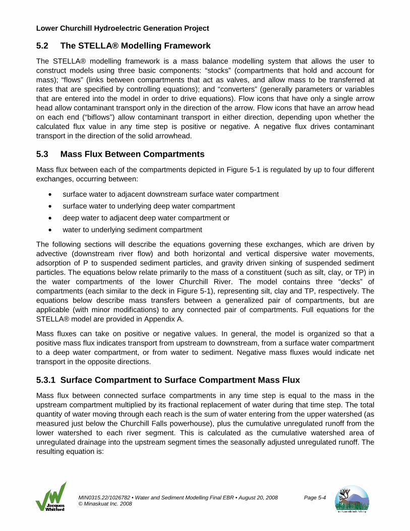
The STELLA® modelling framework is a mass balance modelling system that allows the user to construct models using three basic components: “stocks” (compartments that hold and account for mass); “flows” (links between compartments that act as valves, and allow mass to be transferred at rates that are specified by controlling equations); and “converters” (generally parameters or variables that are entered into the model in order to drive equations). Flow icons that have only a single arrow head allow contaminant transport only in the direction of the arrow. Flow icons that have an arrow head on each end (“biflows”) allow contaminant transport in either direction, depending upon whether the calculated flux value in any time step is positive or negative. A negative flux drives contaminant transport in the direction of the solid arrowhead.
5.3 Mass Flux Between Compartments
Mass flux between each of the compartments depicted in Figure 5-1 is regulated by up to four different exchanges, occurring between:
• surface water to adjacent downstream surface water compartment
• surface water to underlying deep water compartment
• deep water to adjacent deep water compartment or
• water to underlying sediment compartment
The following sections will describe the equations governing these exchanges, which are driven by advective (downstream river flow) and both horizontal and vertical dispersive water movements, adsorption of P to suspended sediment particles, and gravity driven sinking of suspended sediment particles. The equations below relate primarily to the mass of a constituent (such as silt, clay, or TP) in the water compartments of the lower Churchill River. The model contains three “decks” of compartments (each similar to the deck in Figure 5-1), representing silt, clay and TP, respectively. The equations below describe mass transfers between a generalized pair of compartments, but are applicable (with minor modifications) to any connected pair of compartments. Full equations for the STELLA® model are provided in Appendix A.
Mass fluxes can take on positive or negative values. In general, the model is organized so that a positive mass flux indicates transport from upstream to downstream, from a surface water compartment to a deep water compartment, or from water to sediment. Negative mass fluxes would indicate net transport in the opposite directions.
5.3.1 Surface Compartment to Surface Compartment Mass Flux
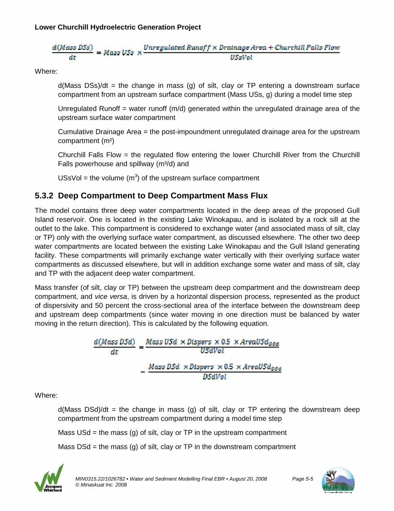
Mass flux between connected surface compartments in any time step is equal to the mass in the upstream compartment multiplied by its fractional replacement of water during that time step. The total quantity of water moving through each reach is the sum of water entering from the upper watershed (as measured just below the Churchill Falls powerhouse), plus the cumulative unregulated runoff from the lower watershed to each river segment. This is calculated as the cumulative watershed area of unregulated drainage into the upstream segment times the seasonally adjusted unregulated runoff. The resulting equation is:
Lower Churchill Hydroelectric Generation Project
MIN0315.22/1026782 • Water and Sediment Modelling Final EBR • August 20, 2008 Page 5-5 © Minaskuat Inc. 2008
Where:
d(Mass DSs)/dt = the change in mass (g) of silt, clay or TP entering a downstream surface compartment from an upstream surface compartment (Mass USs, g) during a model time step
Unregulated Runoff = water runoff (m/d) generated within the unregulated drainage area of the upstream surface water compartment
Cumulative Drainage Area = the post-impoundment unregulated drainage area for the upstream compartment (m²)
Churchill Falls Flow = the regulated flow entering the lower Churchill River from the Churchill Falls powerhouse and spillway (m³/d) and
USsVol = the volume (m3) of the upstream surface compartment
5.3.2 Deep Compartment to Deep Compartment Mass Flux
The model contains three deep water compartments located in the deep areas of the proposed Gull Island reservoir. One is located in the existing Lake Winokapau, and is isolated by a rock sill at the outlet to the lake. This compartment is considered to exchange water (and associated mass of silt, clay or TP) only with the overlying surface water compartment, as discussed elsewhere. The other two deep water compartments are located between the existing Lake Winokapau and the Gull Island generating facility. These compartments will primarily exchange water vertically with their overlying surface water compartments as discussed elsewhere, but will in addition exchange some water and mass of silt, clay and TP with the adjacent deep water compartment.
Mass transfer (of silt, clay or TP) between the upstream deep compartment and the downstream deep compartment, and vice versa, is driven by a horizontal dispersion process, represented as the product of dispersivity and 50 percent the cross-sectional area of the interface between the downstream deep and upstream deep compartments (since water moving in one direction must be balanced by water moving in the return direction). This is calculated by the following equation.
Where:
d(Mass DSd)/dt = the change in mass (g) of silt, clay or TP entering the downstream deep compartment from the upstream compartment during a model time step
Mass USd = the mass (g) of silt, clay or TP in the upstream compartment
Mass DSd = the mass (g) of silt, clay or TP in the downstream compartment
Lower Churchill Hydroelectric Generation Project
MIN0315.22/1026782 • Water and Sediment Modelling Final EBR • August 20, 2008 Page 5-6 © Minaskuat Inc. 2008
Dispers = a parameter representing the horizontal dispersivity of water movements between the two compartments (m/d)
AreaUSdDSd = the cross-sectional area of the interface between the upstream deep and the downstream deep compartment (m²)
USdVol = the volume of the upstream compartment (m³) and
DSdVol = the volume of the downstream compartment (m³)
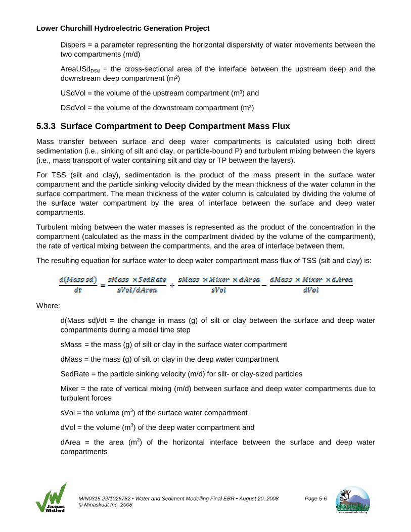
5.3.3 Surface Compartment to Deep Compartment Mass Flux
Mass transfer between surface and deep water compartments is calculated using both direct sedimentation (i.e., sinking of silt and clay, or particle-bound P) and turbulent mixing between the layers (i.e., mass transport of water containing silt and clay or TP between the layers).
For TSS (silt and clay), sedimentation is the product of the mass present in the surface water compartment and the particle sinking velocity divided by the mean thickness of the water column in the surface compartment. The mean thickness of the water column is calculated by dividing the volume of the surface water compartment by the area of interface between the surface and deep water compartments.
Turbulent mixing between the water masses is represented as the product of the concentration in the compartment (calculated as the mass in the compartment divided by the volume of the compartment), the rate of vertical mixing between the compartments, and the area of interface between them.
The resulting equation for surface water to deep water compartment mass flux of TSS (silt and clay) is:
Where:
d(Mass sd)/dt = the change in mass (g) of silt or clay between the surface and deep water compartments during a model time step
sMass = the mass (g) of silt or clay in the surface water compartment
dMass = the mass (g) of silt or clay in the deep water compartment
SedRate = the particle sinking velocity (m/d) for silt- or clay-sized particles
Mixer = the rate of vertical mixing (m/d) between surface and deep water compartments due to turbulent forces
sVol = the volume (m3) of the surface water compartment
dVol = the volume (m3) of the deep water compartment and
dArea = the area (m2) of the horizontal interface between the surface and deep water compartments
Lower Churchill Hydroelectric Generation Project
MIN0315.22/1026782 • Water and Sediment Modelling Final EBR • August 20, 2008 Page 5-7 © Minaskuat Inc. 2008
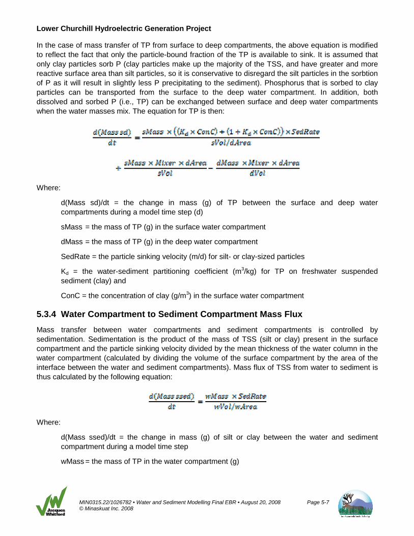
In the case of mass transfer of TP from surface to deep compartments, the above equation is modified to reflect the fact that only the particle-bound fraction of the TP is available to sink. It is assumed that only clay particles sorb P (clay particles make up the majority of the TSS, and have greater and more reactive surface area than silt particles, so it is conservative to disregard the silt particles in the sorbtion of P as it will result in slightly less P precipitating to the sediment). Phosphorus that is sorbed to clay particles can be transported from the surface to the deep water compartment. In addition, both dissolved and sorbed P (i.e., TP) can be exchanged between surface and deep water compartments when the water masses mix. The equation for TP is then:
Where:
d(Mass sd)/dt = the change in mass (g) of TP between the surface and deep water compartments during a model time step (d)
sMass = the mass of TP (g) in the surface water compartment
dMass = the mass of TP (g) in the deep water compartment
SedRate = the particle sinking velocity (m/d) for silt- or clay-sized particles
Kd = the water-sediment partitioning coefficient (m3/kg) for TP on freshwater suspended sediment (clay) and
ConC = the concentration of clay (g/m3) in the surface water compartment
5.3.4 Water Compartment to Sediment Compartment Mass Flux
Mass transfer between water compartments and sediment compartments is controlled by sedimentation. Sedimentation is the product of the mass of TSS (silt or clay) present in the surface compartment and the particle sinking velocity divided by the mean thickness of the water column in the water compartment (calculated by dividing the volume of the surface compartment by the area of the interface between the water and sediment compartments). Mass flux of TSS from water to sediment is thus calculated by the following equation:
Where:
d(Mass ssed)/dt = the change in mass (g) of silt or clay between the water and sediment compartment during a model time step
wMass = the mass of TP in the water compartment (g)

Lower Churchill Hydroelectric Generation Project
MIN0315.22/1026782 • Water and Sediment Modelling Final EBR • August 20, 2008 Page 5-8 © Minaskuat Inc. 2008
wVol = the volume of the water compartment (m³) and
wArea = the area of the interface (m2) between the water and sediment compartments
In the case of mass transfer of TP from water to sediment compartments, sedimentation is modified to reflect the fact that only P that is sorbed to suspended sediment (clay) particles is transported to the sediment compartment. In this case the equation becomes:
5.4 Values Used in the Model
The following section describes the source or the methods used in determining various inputs used in the modelling exercise. The model was designed to initiate on January 1 of the year following impoundment of the reservoir. Values for initial TSS and TP during impoundment cannot be accurately modelled.
5.4.1 Geographic Information System Measurements
The Geographic Information System (GIS) software used for spatial data interpretation was ESRI ArcGIS ArcINFO 9.2. The ESRI ArcGIS 3D Analyst extension was also used in working with the LiDAR data used to generate existing conditions for river bathymetry and corresponding volumes. Biomass estimates were derived from ecological land classifications (ELC) (Minaskuat 2007b) and forest inventories (EnFor 2008); coverage areas were calculated on a 2-dimensional basis. Data generated using the GIS are listed in Table 5-1 and were generated by using spatial analysis tools within GIS. This was achieved by intersecting layers of interest and spatially querying areas and features of interest to fulfill required criteria. A partial list of GIS data sources used is as follows:
1. 1:500,000 Earth Observation for Sustainable Development (EOSD, NRCan) Description: Land Cover Classification Source: Natural Resources Canada, Canadian Forest Service - Atlantic Forestry Centre Publication date: 2006
2. 1:50,000 Watersheds (Geogratis) Description: Watershed boundaries for the project area Source: Original data downloaded from Geogratis and modified by Stephen Rowe Publication Date: Undated
3. 1:50,000 Catchment Areas (created by Minaskuat 2007b) Description: Sub Watershed units based on the Churchill River project reaches. Source: Minaskuat interpreted from digital terrain using ArcGIS software Created: 2007
4. 1:250,000 National Topographic System (NTS, NRCan) Projection: 'NAD_1983_UTM_Zone_20N' Source: Natural Resources Canada Publication Date: Undated


Lower Churchill Hydroelectric Generation Project
MIN0315.22/1026782 • Water and Sediment Modelling Final EBR • August 20, 2008 Page 5-9 © Minaskuat Inc. 2008
Table 5-1 Data Generated by GIS Catchment Areas Including Phosphorus, Silt and Clay Loadings

Lower Churchill Hydroelectric Generation Project
MIN0315.22/1026782 • Water and Sediment Modelling Final EBR • August 20, 2008 Page 5-10 © Minaskuat Inc. 2008
5. 1:20,000 ELC (Created by Minaskuat in 2007 from new colour orthophotography) Description: Ecological Land Classification (ELC) Source: Minaskuat interpreted from colour orthophotography Created: 2007
The information depicted in this GIS layer is the result of digital analyses performed on a database consisting of information from a variety of governmental and other reliable sources. The accuracy of the information presented is limited to the collective accuracy of the database on the date of the analysis. The information is believed accurate and reasonable efforts have been made to ensure the accuracy of the data.
5.4.2 Surface Compartment Loading
Each of the eight surface water compartments were modelled to account for loading of surface water through regulated and unregulated runoff, silt, clay and P loading through shoreline erosion and P loading through plant matter decomposition and flooded soil leaching. The process used to calculate regulated and unregulated runoff is described in Sections 5.4.5 and 5.4.6, respectively.
Estimates of shoreline Erosion Potential were drawn from AMEC (2007). Minaskuat then used GIS to calculate average erosion volumes for each model reach based on the AMEC (2007) estimates of slope, erodability, and wave energy. Erosion Potential takes into consideration shoreline stability, soil types, fetch and exposure to wave action. Each model segment is assigned a unique sediment loading based on these variables. Sediment loading to the reservoir segments is assumed to occur at a uniform rate during the ice-free season, and to fall to zero (due to the absence of wave action and the stabilizing effect of freezing on lake shorelines) during the winter period.
The Shoreline Erosion Intensity parameter (unitless) was used to modify the Erosion Potential (m3/d) over time. The Shoreline Erosion Intensity is assigned a value of 1.0 in the first two years following impoundment, and is allowed to decline thereafter to a minimum value of 0.05 after 20 years. Values were selected based on professional judgment; however, it is important to note that the worst-case conditions will occur when the Shoreline Erosion Intensity has a value of 1.0. This represents a worst-case situation, since the Erosion Potential is, as its name indicates, a measure of the potential for erosion, and not an indicator that the potential erosion rate will be realized at all locations or at all times (it will be modified by such factors as actual wave energy and water levels).
Loading of silt and clay to the surface water compartments was derived by multiplying the calculated erosion volumes by the percent fraction of silt and clay expected in the eroded soils. These fractions were derived from the ELC soil distribution maps generated by Minaskuat (2007b). Lastly, silt and clay loading values were multiplied by the Shoreline Erosion Intensity parameter to account for the reduced erosion activity expected as shorelines reach new equilibrium.
Phosphorus loading to the surface water compartments is linked to soil erosion and biomass decomposition; these processes are described in Sections 5.4.3 and 5.4.7.
Lower Churchill Hydroelectric Generation Project
MIN0315.22/1026782 • Water and Sediment Modelling Final EBR • August 20, 2008 Page 5-11 © Minaskuat Inc. 2008
5.4.3 Biomass Decomposition Rate Calculations
Following impoundment, the biomass remaining in the flooded areas will decompose and release P into the aquatic system. The rate at which biomass decomposes will in part determine the magnitude of P loading to the reservoirs and therefore the degree of potential eutrophication of the system. The decomposition of vegetation and organic matter typically occurs in three stages based on the types of organic compounds present (Westrich and Berner 1984; Carignan and Lean 1991). Lignin, cellulose and protein have been shown to be differentially labile with respect to bacterial decomposition (Westrich and Berner 1984). Highly reactive compounds decompose rapidly (i.e., days to weeks, Carignan and Lean 1991) and will generally be lost from the soil litter and duff layers in the period between clearing and flooding of the reservoirs. Any of the remaining highly reactive components will likely be eliminated from the reservoirs during the initial flooding period. These compounds are also primarily mono- and polysaccharide structures that contain very low concentrations of P. Unreactive components (i.e., lignins, resins, and waxes) have slow decomposition rates (k = 0.01/yr) that render the decomposition of these compounds a minor component of the TP released from decomposition of organic matter. Therefore, the TSS and TP model focuses on the moderately reactive component of the flooded organic matter because it will determine the rate of P release into the reservoir system. As part of the overall conservative approach, it was assumed that all vegetative biomass remaining in the flood zone would decompose at a moderately reactive rate.
Decomposition of organic matter was modelled using a first-order exponential decay model, which is explained by the following equation:
Mt = M0 e-kt
Where: Mt is the biomass (kg) at time t, M0 is the biomass (kg) at the starting time, t is the time elapsed (yr), and k is the decomposition rate (1/yr).
In the model, the default decomposition rate is set at 0.3/yr during the ice-free period when water is warm and 0.074 during the ice-cover period. These values are converted to values of 0.000822/d and 0.000205/d (units of “per day”, respectively in the STELLA® model). Justification for using these default values and the alternate values in the sensitivity analysis is provided in Section 5.5.7.
5.4.4 Ice-free Season
Estimates of shoreline erosion are based on data provided in the Bank Stability Study (AMEC 2007). Erosion Potential takes into consideration shoreline stability, soil types, fetch and exposure to wave action. Sediment loading to the reservoir segments is assumed to occur at a uniform rate during the ice-free season, and to fall to zero (due to the absence of wave action and the stabilizing effect of freezing on lake shorelines) during the winter period. For this reason, estimating the period when the water bodies are free of ice is essential to the TSS and TP model.
In the Ice Dynamics Study Draft Report, Hatch (2007) describes that freezing in Goose Bay generally begins in late October or early November and that thawing begins somewhere between mid-April to mid-May. Hatch (2007) goes on to describe that due to the ability of large water bodies to act as thermal capacitors, the creation of the reservoirs will delay the freezing and thawing processes by approximately two weeks. As a result, the ice-free season for the Churchill River was defined to start on May 15 and to end on November 26, for a total duration of 196 days.

Lower Churchill Hydroelectric Generation Project
MIN0315.22/1026782 • Water and Sediment Modelling Final EBR • August 20, 2008 Page 5-12 © Minaskuat Inc. 2008
5.4.5 Regulated Flow Volumes
The head of the Churchill River is the Smallwood Reservoir. This reservoir was created by damming the river and hence creating a control structure as part of the Churchill Falls Hydroelectric Development. Water escapes the reservoir and enters the lower Churchill River, either though the powerhouse as part of the power generation process or the spillway as excess water. A river gauging station (EC 03OD005) located just downstream of the Churchill Falls Hydroelectric Development powerhouse and the spillway measures the volume of water entering the lower Churchill River. These volumes are recorded and available from Environment Canada and were used to determine average monthly regulated flow volumes entering the river (Table 5-2). These values vary monthly and are recorded in the STELLA® model as a graphical function linked to Julian days. Regulated flow volumes are repeated each year and are not modified for potential changes in long-term weather patterns.
Table 5-2 Monthly Mean Flow Rates at Gauging Station EC 03OD005
Month Flow (m³/d)
January 1.44E+08 February 1.41E+08 March 1.29E+08 April 1.12E+08 May 9.50E+07 June 9.50E+07 July 9.94E+07 August 1.00E+08 September 9.94E+07 October 1.09E+08 November 1.24E+08 December 1.40E+08
5.4.6 Unregulated Flow Volumes
Unregulated runoff is considered to be the amount of surface water entering the Churchill River through natural water courses and overland flow. It is a product of rainfall and is affected by evaporation, transpiration and groundwater recharge. These parameters could be estimated for the lower Churchill River watershed with some certainty. Alternatively, net freshwater input into the river system can be estimated using data from monitoring stations along the river. Environment Canada publishes average monthly flows from various monitoring locations throughout the country. Two of these locations are present at the Churchill Falls Hydroelectric Development powerhouse (EC 03OD005) and above Muskrat Falls (EC 03OE001). The Unregulated Flow rate can be calculated by dividing the net flow through the river (flow at Muskrat Falls less flow just below Churchill Falls outlet) by the watershed drainage area upstream of Muskrat Falls. This indicates the amount of precipitation that fell on a unit of the watershed and reached Muskrat Falls and hence, takes into account losses to evaporation, transpiration and groundwater recharge. The monthly mean unregulated runoff rates (m/d) for the lower Churchill River are provided in Table 5-3. By assuming that the watershed below Muskrat Falls is similar in climate, geology and vegetation as the watershed above Muskrat Falls, the unregulated flow volumes for the entire watershed can be estimated. Both the extent of the Churchill River watershed and the incremental extent of each catchment area (corresponding to the eight reaches used in the model) are depicted in Figure 5-1. The size of each catchment area was derived using GIS software
Lower Churchill Hydroelectric Generation Project
MIN0315.22/1026782 • Water and Sediment Modelling Final EBR • August 20, 2008 Page 5-13 © Minaskuat Inc. 2008
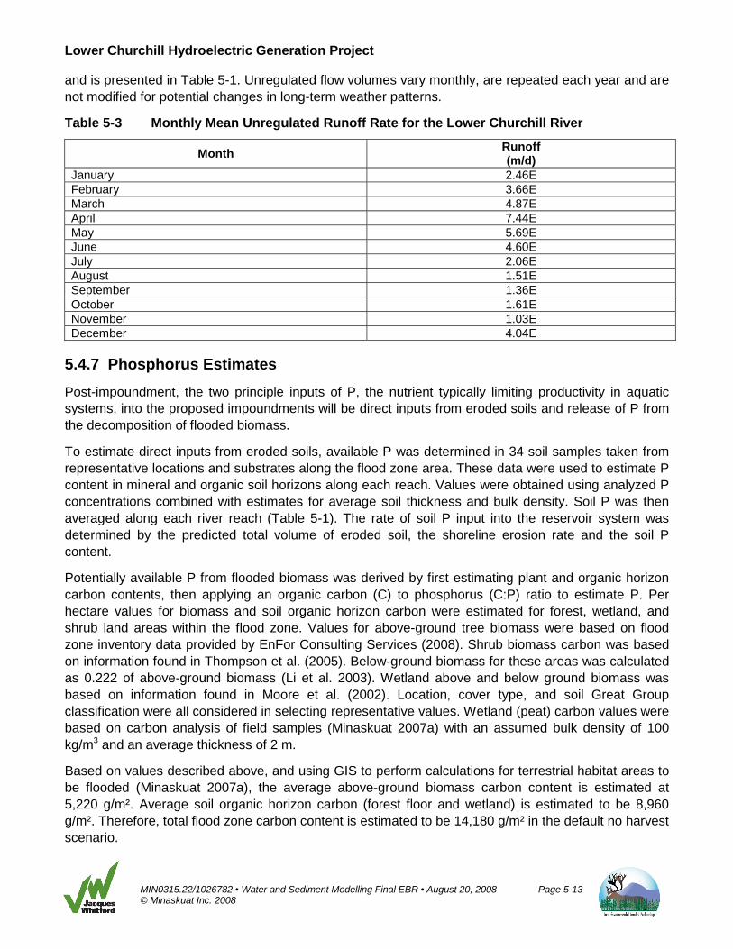
and is presented in Table 5-1. Unregulated flow volumes vary monthly, are repeated each year and are not modified for potential changes in long-term weather patterns.
Table 5-3 Monthly Mean Unregulated Runoff Rate for the Lower Churchill River
Month Runoff (m/d)
January 2.46E February 3.66E March 4.87E April 7.44E May 5.69E June 4.60E July 2.06E August 1.51E September 1.36E October 1.61E November 1.03E December 4.04E
5.4.7 Phosphorus Estimates
Post-impoundment, the two principle inputs of P, the nutrient typically limiting productivity in aquatic systems, into the proposed impoundments will be direct inputs from eroded soils and release of P from the decomposition of flooded biomass.
To estimate direct inputs from eroded soils, available P was determined in 34 soil samples taken from representative locations and substrates along the flood zone area. These data were used to estimate P content in mineral and organic soil horizons along each reach. Values were obtained using analyzed P concentrations combined with estimates for average soil thickness and bulk density. Soil P was then averaged along each river reach (Table 5-1). The rate of soil P input into the reservoir system was determined by the predicted total volume of eroded soil, the shoreline erosion rate and the soil P content.
Potentially available P from flooded biomass was derived by first estimating plant and organic horizon carbon contents, then applying an organic carbon (C) to phosphorus (C:P) ratio to estimate P. Per hectare values for biomass and soil organic horizon carbon were estimated for forest, wetland, and shrub land areas within the flood zone. Values for above-ground tree biomass were based on flood zone inventory data provided by EnFor Consulting Services (2008). Shrub biomass carbon was based on information found in Thompson et al. (2005). Below-ground biomass for these areas was calculated as 0.222 of above-ground biomass (Li et al. 2003). Wetland above and below ground biomass was based on information found in Moore et al. (2002). Location, cover type, and soil Great Group classification were all considered in selecting representative values. Wetland (peat) carbon values were based on carbon analysis of field samples (Minaskuat 2007a) with an assumed bulk density of 100 kg/m3 and an average thickness of 2 m.
Based on values described above, and using GIS to perform calculations for terrestrial habitat areas to be flooded (Minaskuat 2007a), the average above-ground biomass carbon content is estimated at 5,220 g/m². Average soil organic horizon carbon (forest floor and wetland) is estimated to be 8,960 g/m². Therefore, total flood zone carbon content is estimated to be 14,180 g/m² in the default no harvest scenario.

Lower Churchill Hydroelectric Generation Project
MIN0315.22/1026782 • Water and Sediment Modelling Final EBR • August 20, 2008 Page 5-14 © Minaskuat Inc. 2008
Assuming an organic matter C:P molar ratio of 500:1 (Prescott et al. 2004), and considering the atomic masses of carbon and P (12 and 31, respectively), the organic matter C:P mass ratio becomes 6,000:31 or roughly 200:1. As a result, the average flood zone P inventory is estimated to be 71 g/m².
The best estimate model does not include tree harvesting and reservoir clearing. However, the effect of both clearing scenarios are evaluated in the sensitivity analysis (see Sections 5.5.9, 6.2.2, and 6.3.2).
5.4.8 Settling Velocities for Silt and Clay
Fine particles added to the water column through shoreline erosion or other inputs have two possible fates: suspended particles may flow through the river reach as they pass through the watercourse, or they may sink and deposit on the lake or river bottom. Fine particles, such as clay, settle at a slower rate, thus remaining suspended in the water column for longer than large coarse particles, such as sand and gravel. Indeed, suspended sediment fate and concentrations are heavily influenced by settling velocities of the sediments in the water column. In typical lakes and rivers, suspended sediment is comprised of particles finer than 74 µm (primarily silt and clay, Newcombe 1994).
As coarse matter and sand settles very rapidly, they were not considered to contribute to TSS in the water column. Therefore, representative settling rates for silt and clay were required. Sullivan et al. (2007) assigned two settling rates, 21 m/d for particles 2 µm (representing silt), and 0.6 m/d for particles <2 µm (representing clay) in order to model suspended sediment in an impoundment in Oregon. These values are comparable to, although slightly higher than those calculated using Stokes’ Law. Differences between empirically measured settling velocities and those measured in the laboratory or calculated using Stokes’ Law can be caused by uncertainty regarding the actual shapes of particles (irregularly shaped or flattened particles may sink more slowly than spherical particles), or processes that cause particles to agglomerate and sink more quickly than would otherwise be predicted. Settling velocities of 21 m/d for silt and 0.6 m/d for clay were used in the STELLA® model.
5.4.9 Vertical Mixing and Deep Water Dispersion Coefficients
The vertical mixing coefficient is represented in the model as the variable “Mixer” and is used to simulate vertical mixing of the water column in the deeper portions of the reservoir system, specifically in Lake Winokapau, and in the two downstream segments representing the Gull Island reservoir.
Mixing in freshwater lakes is typically driven by wind, and is impeded by ice cover in winter and by thermal stratification in winter and summer. It was assumed that the deeply impounded segments would stratify thermally during the winter. The formation of ice cover will eliminate wind forcing during the winter, therefore vertical mixing during the winter will be negligible. It was also assumed that for a period of 15 days following ice-out in spring, and 30 days prior to freeze-up in the fall, the reservoirs will be isothermal with depth, and resistance to vertical mixing will be minimal. During the summer period, there is weak thermal stratification that impedes mixing, although the thermocline is typically weak and deep (around 25 m depth) in Lake Winokapau under present day conditions. Mixer was assigned a value of 0.26 m/d from Julian day 0 to 135 (representing winter ice cover), 90 m/d from days 135 to 149 (representing spring turnover), 1 m/d from days 150 to 300 (representing limited mixing in a stratified system during summer), 90 m/d from days 301 to 330 (representing fall turnover), and 0.26 m/d from days 331 to 365 (representing minimal mixing due to winter ice cover). These values are repeated each year.
Lower Churchill Hydroelectric Generation Project
MIN0315.22/1026782 • Water and Sediment Modelling Final EBR • August 20, 2008 Page 5-15 © Minaskuat Inc. 2008
Most of the newly impounded river will remain dominated by advective flows from upstream to downstream, particularly in the surface water layer. In Lake Winokapau, there currently is, and post-impoundment there will remain, a deep-water compartment (WD) that is somewhat isolated from the river flow during periods of thermal stratification. In addition, post-impoundment, there will be two segments in the Gull Island reservoir (i.e., G1D and G2D) that are relatively isolated from advective flows because the Gull Island reservoir will be a deep impoundment (roughly 100 m deep near the generating facility) water body with surface drawdown. In contrast, the Muskrat Falls reservoir will be less deep, and will have bottom drawdown, so there will be low potential for stratification and isolation of a deep water compartment at Muskrat Falls.
The deep water compartment in Lake Winokapau will remain isolated from the downstream portions of the Gull Island reservoir by a bedrock sill at the outflow of the lake. In contrast, the deep water compartments at Gull Island (G1D and G2D) will be connected to each other, and even in the absence of advective water movements, there will be exchange of water between these two compartments by eddy dispersion. Horizontal mixing in stratified lakes is substantially more rapid than vertical mixing, although vertical mixing will approach the rate of horizontal mixing during spring and fall overturn. The variable “Dispers” is used to represent this process, and has been assigned a best estimate value of 162 m/d.
5.5 Model Sensitivity Analysis
The TSS and TP model is sensitive to the values of all input parameters; however, most parameter values (such as watershed areas and reservoir segment volumes) are considered to be known with a high level of confidence, or are invariant. As such, these parameters have fixed values (or seasonal ranges of values) and need not be investigated with respect to the sensitivity of model outputs. The following section reviews the parameters included in the model which are not known with certainty, or which may vary substantially, and for which the selection of standard values may affect the model outputs. With several parameters having some degree of uncertainty and an assigned probable range of values the potential individual and cumulative effects of varying these parameters was investigated.
Initially, the effect of varying one parameter value was investigated while each other parameter was set at its best estimate value. Subsequently, each parameter was set to the value at the limit of its probable range that would produce the highest concentration of TSS or TP and the model was run to determine the worst-case scenario. In order to compare the predicted outcomes with the best-case scenario, the selected variables were all set to the value that would cause the minimum concentration of TSS and TP. As peak concentrations of TSS and TP occur in the first year post-impoundment, the effect of varying the sensitivity analysis parameters was examined over the first 365-day period. The best estimate, minimum and maximum probable values of variables identified as key variables to test in the sensitivity analysis are presented in Table 5-4. In order to further simplify the sensitivity analysis, the effects of varying the six key parameters (i.e., river flow rate, organic matter decomposition rate, Kd for P on TSS, particle settling velocities, vertical and horizontal mixing or dispersion rates, and flooded biomass) were examined in the most sensitive reaches of both the Gull Island and Muskrat Falls reservoirs (i.e., model segments G2S and ML3, see Figure 5-1).

Lower Churchill Hydroelectric Generation Project
MIN0315.22/1026782 • Water and Sediment Modelling Final EBR • August 20, 2008 Page 5-16 © Minaskuat Inc. 2008
Table 5-4 Minimum, Best Estimate, and Maximum Parameter Values for Model Sensitivity Analysis
Parameter Effect on TSS or TP
Low Range
Best Estimate
High Range
River Flow Rate (multiplier) +/-A 0.786 1 1.286 Decomposition Rate (multiplier) + 0.667 1 1.333 Kd for P on TSS (values) - 300 600 900 Particle Settling Velocity (multiplier) + 0.7 1 1.6 Vertical Mixer and Water Dispersion (multiplier)
- 0.333 1 3
Flooded Biomass (values) + 8,960/13,240B 14,180 A River flow rate had a negative effect on TP in both reaches, and a negative effect on TSS only in the Muskrat Falls reservoir reach due to increased flushing and dilution. In Gull Island reservoir it had a small positive effect due to reduced sediment trap efficiency on the deep compartments. B The best estimate value was set to include all flooded vegetation. The Low Range value for this parameter tests both the full clearing scenario and partial clearing scenario (8,960/13,240), and the best-case scenario uses the full clearing value of Flooded Biomass.
The two extreme scenarios (i.e., worst-case and best-case) effectively comprise the upper and lower confidence limits of the best estimate scenario. The best estimate scenario is a result of the parameters set to values estimated based on available literature and professional judgment. The probability that either the worst or best-case scenario will occur is low as they represent the product of the probabilities that all of the parameter values will assume the stipulated maximum or minimum values simultaneously. The one exception to this approach was the flooded biomass value. The best estimate and worst case scenarios converge, as it was assumed (conservatively) for these scenarios that there will be no harvesting or clearing of the flood zones, and the flooded biomass estimate for these scenarios was 14,180 g C/m2. The best-case scenario involves the flooded biomass set to a value of 8,960 g C/m2 following the removal of all above-ground biomass under the Full Clearing scenario as described in Section 5.5.9. The effect of Partial Clearing on TP concentrations is also assessed, but this scenario is not used to determine the best-case scenario.
The justification for the low range and high range parameter values used in the sensitivity analysis and those parameters that were determined not to be tested in the sensitivity analysis are described in the following sections.
5.5.1 Shoreline Erosion Intensity
Estimates of the Erosion Potential (m3/d) are based on data provided in the Bank Stability Study (AMEC 2007). Factors affecting shoreline erosion are outlined in section 5.4.2.
The Shoreline Erosion Intensity parameter (unitless) is used to modify the Erosion Potential (m3/d) over time. Shoreline Erosion Intensity is assigned a value of 1.0 in the first two years following impoundment, and is allowed to decline thereafter to a minimum value of 0.05 after 20 years. Values were selected based on professional judgment; however, it is important to note that the worst-case conditions will occur when Shoreline Erosion Intensity has a value of 1.0. This represents a worst-case condition, since the Erosion Potential identified by AMEC is, as its name indicates, a measure of the potential for erosion, and not an indicator that the potential erosion rate that will be realized at all locations or at all times (since it will be modified by such factors as actual wave energy and water levels). It is possible that peak shoreline erosion intensity may last for longer than the two year period

Lower Churchill Hydroelectric Generation Project
MIN0315.22/1026782 • Water and Sediment Modelling Final EBR • August 20, 2008 Page 5-17 © Minaskuat Inc. 2008
used in the model. Again, this would not result in higher concentrations of TSS or TP in the reservoirs, but would result in an extended period of time when these peak concentrations would be observed.
While the exact time frame required for stabilization of the new shorelines cannot be known in advance, the scenario that has been developed (i.e., worst-case erosion rates during the first two years following impoundment, with erosion rates subsequently declining to a base level after 20 years) is consistent with experience elsewhere, and will not result in an under-estimate of worst-case conditions. Ragozin and Burova (1993) described three phases of erosion with the initial phase being intense (intensity = 1) and lasting approximately four years in sandy terrain (range two to seven years). The second phase of erosion has a longer duration (perhaps 10 to 20 years) and is less intense (intensity approximately 0.3 to 0.4) than the initial phase, and transitions into the third and longest phase of erosion, when shorelines are approaching stability and erosion intensity is low (intensity < 0.1). The time scale of the erosion intensity curve used in the model is consistent with median values for the erosion of sandy shorelines from Ragozin and Burova (1993), with erosion intensity reaching a value of 0.1 by year 13. It is possible that the time scale of the erosion intensity curve could be prolonged, or that peak erosion intensity would not occur until the second or even several years post-impoundment due to the protective effect of shoreline vegetation on its stability. However, shoreline erosion rates from Baskatong Reservoir, Quebec, (Saint-Laurent et al. 2001) and from Southern Indian Lake, Manitoba, (Newbury and McCullough 1984) indicate that shoreline recession was most significant immediately following impoundment. However, an extended erosion intensity curve, or a lag in peak erosion intensity, would not affect the peak concentration of TSS or TP, but would simply cause a delay in the peak concentration. Therefore, no manipulation of the shoreline erosion intensity is required for sensitivity analysis.
5.5.2 Baseline Total Suspended Solids Concentration in Water and Silt and Clay Fractions
Baseline concentrations of TSS in water are based on values reported in water quality surveys (Minaskuat 2007a). Baseline concentrations of TSS are typically low (<5 mg/L) in the upper river (above Gull Island) but increase in the lower reaches of the river due to erosion of the predominantly sandy shorelines. Baseline concentrations of TSS in the lower river also display higher concentrations during spring (11 to 127 mg/L) when runoff from the watershed typically increases, water levels are high, and erosion rates increase. The TSS in the lower river has been linked to an increase in mineral particles (clay and silt) in suspension in the river water (Minaskuat 2007a). The baseline concentration of TSS in water entering the river from the Smallwood Reservoir or tributaries to the Churchill River is therefore assumed to be 1 mg/L, with 10 percent of this amount being clay-sized, and 90 percent being silt-sized particles based on soil quality data from the watershed. Variation in the baseline TSS concentration in water, or the fractionation between silt and clay will have a negligible effects on model outputs, since the model-predicted silt and clay concentrations are much higher, and are dominated by materials originating from soil erosion.
For eroded soils, the clay and silt fraction is empirically determined, and varies from 0.21 percent clay (as a fraction of the TSS) to 31.5 percent clay. These fractions were determined based on soils data and soil types in the various reaches (from GIS), and are considered to be reliably known. Therefore, no manipulation of the clay and silt fraction is required for sensitivity analysis.

Lower Churchill Hydroelectric Generation Project
MIN0315.22/1026782 • Water and Sediment Modelling Final EBR • August 20, 2008 Page 5-18 © Minaskuat Inc. 2008
5.5.3 Baseline Phosphorus Concentration in Water
TP concentrations in the Churchill River vary along the length of the river and by season. Data from Lake Winokapau indicate a generally oligotrophic state, with TP ranging from 0.006 to 0.012 mg/L, with a mean of 0.009 mg/L (Minaskuat 2007a). The middle section of the river had TP concentrations similar to Lake Winokapau, ranging over the year from 0.006 to 0.019 mg/L with a mean of 0.01 mg/L (Minaskuat 2007a). The lower reaches of the river (below the proposed Gull Island generating facility) typically have higher concentrations of TP, ranging from 0.012 to 0.034 mg/L in the fall, and 0.018 to 0.152 mg/L in the late winter and spring (Minaskuat 2007a). These increases (both upstream to downstream, and seasonally) are probably due to nutrient inputs associated with erosion, and during the spring thaw. These processes will be substantially modified post-impoundment, since shoreline erosion intensity in the reservoirs will be driven by wave action, not by water velocities in the free-flowing river. Since the water flow in the lower river is dominated by water discharged from the Smallwood Reservoir (with low TP), and by tributaries draining relatively pristine land, the baseline TP concentrations in all water entering the proposed reservoirs in the lower Churchill River is assumed to be 0.01 mg/L.
5.5.4 Vertical Mixing (Mixer) and Deep Water Dispersion (Dispers)
The variable Mixer is used to simulate vertical mixing of the water column in the deeper portions of the reservoir system, specifically in Lake Winokapau, and in the two downstream segments representing the Gull Island reservoir. In the absence of mixing, the upper and lower water layers would be completely independent and the lower water layers would be stagnant. The variable Dispers is used to simulate exchange between deep water compartments of Lake Winokapau.
The high mixing rates in spring and fall simulate spring and fall overturn of the water bodies, bringing the TSS and TP concentrations of the upper and lower water masses to relatively uniform concentrations. The lower mixing rates in the summer partially segregate the water masses, although particles of silt and clay continue to sink from the upper water layer to the lower water layer, and the clay particles are assumed to carry some adsorbed P down to the lower water layer. Vertical mixing rates in the winter, spring and fall are not likely to be subject to variation in a way that would measurably affect model outputs. There is a high level of confidence that the deep water portions of Lake Winokapau will be stratified and weakly mixing in the winter, and also that the lake undergoes strong mixing in spring and fall. It is assumed that these processes will also apply to the proposed Gull Island reservoir.
For the best estimate scenario, Mixer was assigned a value of 0.26 m/d from Julian day 0 to 135 (representing winter ice cover), 90 m/d from days 135 to 149 (representing spring turnover), 1 m/d from days 150 to 300 (representing limited mixing in a stratified system during summer), 90 m/d from days 301 to 330 (representing fall turnover), and 0.26 m/d from days 331 to 365 (representing minimal mixing due to winter ice cover) (see also Section 5.4.9). These values are repeated each year.
Under the best estimate scenario, Dispers was assigned a value of 162 m/d. When applied to 50 percent of the surface area of the vertical boundary between these two compartments (estimated to be 0.5 × 30,337 m2), the result is an estimated water exchange of 2.46E06 m3/d between the two compartments. Based on the volumes of the two compartments (G1D has a volume of 9.34E08 m3, and G2D has a volume of 1.23E09 m3), this suggests a mixing time of approximately 390 days for the two
Lower Churchill Hydroelectric Generation Project
MIN0315.22/1026782 • Water and Sediment Modelling Final EBR • August 20, 2008 Page 5-19 © Minaskuat Inc. 2008
compartments. Note, however, that strong vertical mixing during spring and fall will cause the two compartments to equilibrate with surface water twice each year.
As these values are based on professional judgment, the sensitivity of the model to varying the Mixer and Dispers values by a factor of 3 was tested. This was done though the variable Mixmaster, which was assigned a default of 1 for the best estimate scenario and alternate low and high values of 0.333 and 3.
5.5.5 Settling Velocities of Silt and Clay
Only silt and clay particles were considered as potential suspended sediments in the water column (See section 5.4.8). These particles classes were assigned settling rates of 21 m/d and 0.6 m/d, respectively, based on the report by Sullivan et al. (2007).
However, Cooke et al. (1993, in Kerr 1995) provided settling velocities for various particles sizes. Silt settling velocities varied from 224 m/d for coarse silt to 0.95 m/d for very fine silt (mean = 47.3 m/d). Clay was broadly given a settling velocity of <0.95 m/d. These settling velocities are faster than those used in the model, and would result in lower estimated concentrations of TSS in water. Hill et al. (2000) estimated the actual settling velocity for suspended sediment in Eel River, Nova Scotia, and determined that an overall mean rate of 8.6 m/d explained the observed settling velocity of the suspended sediments in the river (silt and clay sized particles were not distinguished in this evaluation). This was, nevertheless, faster than a theoretically expected value of 3.5 m/d based on the sampled particle size distribution (very fine clay to medium-coarse sand). This difference in settling velocities was thought to be the result of flocculation of the particles, a process whereby several particles bind together to form one large particle, resulting in overall faster settling velocity. Based on these reports, the estimated settling velocities (21 m/d and 0.6 m/d) are likely to be somewhat low, although this is considered to be conservative, as low settling velocities will lead to an over-estimate of the TSS concentration in water. As settling rates may have a significant effect on the TSS concentrations in the river, the model’s sensitivity to this parameter was tested by adjusting the settling velocities for silt and clay by factors of 0.7 (further lowering the settling velocities) and 1.6 (increasing the settling velocities) using the variable Settlemaster, which was assigned a default best-estimate scenario value of 1 (Table 5-5).
5.5.6 Water/Sediment Partition Coefficient (Kd) for Phosphorus
Phosphorus is generally considered to be the limiting nutrient in aquatic systems due to its generally low availability, and the important role it plays in nucleic acids and energy transfer systems, among other processes (Pant and Reddy 2001; House 2003). Thus, TP dynamics in aquatic systems are important determinants of productivity and trophic state. In addition to being rapidly taken up and cycled by phytoplankton and other aquatic biota, P may be adsorbed to suspended sediment particles. It is estimated that only about 5 to 10 percent of the P eroded from continental rock is carried to the oceans in dissolved form. The rest is likely carried as inert P in fluvial detritus (Froelich 1988). This emphasizes the importance of accurately estimating the rate at which P sorbs to particles, which is estimated as the water/sediment partition coefficient (Kd, L/kg). A large Kd value results in greater sorption of P to suspended sediment, and lower dissolved or bioavailable P.
The P sorption capacity of sediment and suspended particles is dependent on many water and sediment characteristics. For example, finer particles have greater surface area per mass and therefore have a greater number of cation exchange sites to bind with P. Therefore, the Kd value is dynamic and
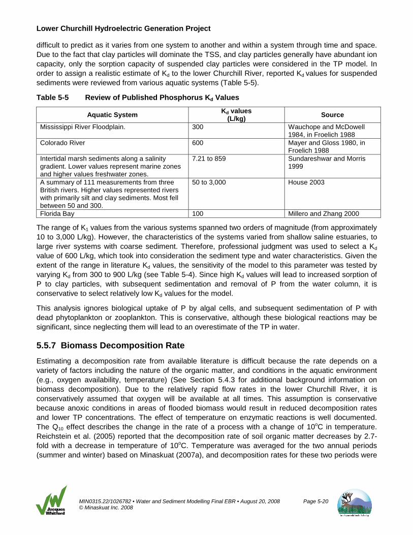
Lower Churchill Hydroelectric Generation Project
MIN0315.22/1026782 • Water and Sediment Modelling Final EBR • August 20, 2008 Page 5-20 © Minaskuat Inc. 2008
difficult to predict as it varies from one system to another and within a system through time and space. Due to the fact that clay particles will dominate the TSS, and clay particles generally have abundant ion capacity, only the sorption capacity of suspended clay particles were considered in the TP model. In order to assign a realistic estimate of Kd to the lower Churchill River, reported Kd values for suspended sediments were reviewed from various aquatic systems (Table 5-5).
Table 5-5 Review of Published Phosphorus Kd Values
Aquatic System Kd values (L/kg) Source
Mississippi River Floodplain. 300 Wauchope and McDowell 1984, in Froelich 1988
Colorado River 600 Mayer and Gloss 1980, in Froelich 1988
Intertidal marsh sediments along a salinity gradient. Lower values represent marine zones and higher values freshwater zones.
7.21 to 859 Sundareshwar and Morris 1999
A summary of 111 measurements from three British rivers. Higher values represented rivers with primarily silt and clay sediments. Most fell between 50 and 300.
50 to 3,000 House 2003
Florida Bay 100 Millero and Zhang 2000
The range of K1 values from the various systems spanned two orders of magnitude (from approximately 10 to 3,000 L/kg). However, the characteristics of the systems varied from shallow saline estuaries, to large river systems with coarse sediment. Therefore, professional judgment was used to select a Kd value of 600 L/kg, which took into consideration the sediment type and water characteristics. Given the extent of the range in literature Kd values, the sensitivity of the model to this parameter was tested by varying Kd from 300 to 900 L/kg (see Table 5-4). Since high Kd values will lead to increased sorption of P to clay particles, with subsequent sedimentation and removal of P from the water column, it is conservative to select relatively low Kd values for the model.
This analysis ignores biological uptake of P by algal cells, and subsequent sedimentation of P with dead phytoplankton or zooplankton. This is conservative, although these biological reactions may be significant, since neglecting them will lead to an overestimate of the TP in water.
5.5.7 Biomass Decomposition Rate
Estimating a decomposition rate from available literature is difficult because the rate depends on a variety of factors including the nature of the organic matter, and conditions in the aquatic environment (e.g., oxygen availability, temperature) (See Section 5.4.3 for additional background information on biomass decomposition). Due to the relatively rapid flow rates in the lower Churchill River, it is conservatively assumed that oxygen will be available at all times. This assumption is conservative because anoxic conditions in areas of flooded biomass would result in reduced decomposition rates and lower TP concentrations. The effect of temperature on enzymatic reactions is well documented. The Q10 effect describes the change in the rate of a process with a change of 10oC in temperature. Reichstein et al. (2005) reported that the decomposition rate of soil organic matter decreases by 2.7-fold with a decrease in temperature of 10oC. Temperature was averaged for the two annual periods (summer and winter) based on Minaskuat (2007a), and decomposition rates for these two periods were
Lower Churchill Hydroelectric Generation Project
MIN0315.22/1026782 • Water and Sediment Modelling Final EBR • August 20, 2008 Page 5-21 © Minaskuat Inc. 2008
determined using these average temperatures. While the intra-annual pattern of water temperature is more variable, this approach was deemed reasonable given the temporal extent of the model.
Carignan and Lean (1991) determined the rate of decomposition for the three classes of organic matter in a mestrophic Canadian Shield lake in Ontario; conditions that would be similar to those in the proposed impoundments. They estimated the decomposition rate for the moderately reactive class of compounds to be 0.2/yr. Root litter decomposition rates from the littoral zone of a boreal lake ranged from 0.19 to 0.3/yr (Larmola et al. 2006). Decomposition rates from a tropical mesotrophic brackish wetland, after correcting for the Q10 effect, were similar and averaged 0.40/yr (Rejmánková and Houdková 2006). The latter rate may be slightly elevated due to the higher trophic status of the brackish wetland compared to the reports from boreal sites, and because of the marine influence as the rate of decomposition within the wetland increased along the salinity gradient. Therefore, the decomposition rate of organic matter in the TSS and TP model was estimated to be 0.3/yr during the open water season when temperatures are relatively warm (i.e., 15°C) and 0.074/yr during the ice-covered period when temperatures are low (0°C). However, as P input from decomposing vegetation may release a large amount of P into the aquatic system, the model sensitivity to this parameter was tested by varying the summer decomposition rate from 0.2/yr to 0.4/yr, values representing the range reported in the literature, and concomitantly the winter values from 0.049/yr to 0.097/yr. This was done through the variable Decaymaster, which varied from the best estimate default value of 1 to low and high values of 0.667 and 1.333 (Table 5-4).
5.5.8 Annual River Flow
The TSS and TP model was based on long-term average river discharge rates measured by Environment Canada at the Churchill Falls tailrace, and at Muskrat Falls, since the 1970s. The effect of altered river flow (corresponding to wet or dry years) was evaluated by modelling the observed maximum and minimum river flow rates on the concentrations of TSS and TP in the river. These extreme scenarios were implemented by adjusting the average flow rate by factors of 1.286 (high river flow) and 0.786 (low river flow) using the variable Wetmaster, which was assigned a default best-estimate scenario value of 1 (Table 5-4).
Altering flow rates would have several potential effects on TSS and TP concentrations. Increased flow rates would decrease retention time of water within the reservoir, which would also decrease settling time of TSS and help to flush TSS and TP downriver (decreased retention). It would also result in increased dilution, which would serve to decrease concentrations of both TSS and TP. Low river flow rates would cause decreased dilution (higher concentrations of TSS and TP in water), but would also allow for increased retention of TSS and TP in reservoir sediments.
5.5.9 Reservoir Clearing
Removal of vegetation was not accounted for in the best estimate model as a conservative approach. However, as two different harvesting scenarios have been proposed (full clearing and partial clearing), the effect of these harvesting scenarios on TP concentrations was tested in the sensitivity analysis. According to the Reservoir Preparation Plan - Update 2007 Draft Report (EnFor 2008), the two harvesting scenarios are defined as follows:
• full clearing and brush disposal: this scenario involves the complete removal and disposal of all vegetation within the proposed flood zone for both the Gull Island and Muskrat Falls reservoirs.

Lower Churchill Hydroelectric Generation Project
MIN0315.22/1026782 • Water and Sediment Modelling Final EBR • August 20, 2008 Page 5-22 © Minaskuat Inc. 2008
Under this scenario merchantable timber would to be salvaged and brush and vegetation removed.
• partial clearing and brush disposal: this scenario applies to the Gull Island Reservoir only and is defined as the preparation of the area between 3 m elevation below low supply level (119 m) and 3 m above full supply level (128 m). This area is commonly referred to as the “Ice-Ring”. The Muskrat Falls Reservoir would be treated the same as under the full clearing scenario.
These harvesting scenarios would not affect the average soil organic horizon carbon value (8,960 g/m2), but would influence the amount of above-ground biomass, estimated to be 5,520 g/m2 on average. As the full clearing scenario implements full tree harvesting and clearing of brush, and the remaining vegetation would be a negligible amount of biomass, the above-ground biomass in both reservoirs was set to 0 g/m2 in this scenario. In the partial clearing scenario, above-ground biomass in the Muskrat Falls reservoir was set to 0 g/m2, but was set to 4,280 g/m2 in the Gull Island reservoir to account for harvesting and clearing down to 3 m below low supply level. (119 m asl).
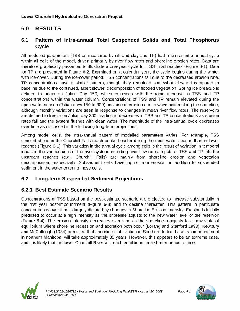
Lower Churchill Hydroelectric Generation Project
MIN0315.22/1026782 • Water and Sediment Modelling Final EBR • August 20, 2008 Page 6-1 © Minaskuat Inc. 2008
6.0 RESULTS
6.1 Pattern of Intra-annual Total Suspended Solids and Total Phosphorus Cycle
All modelled parameters (TSS as measured by silt and clay and TP) had a similar intra-annual cycle within all cells of the model, driven primarily by river flow rates and shoreline erosion rates. Data are therefore graphically presented to illustrate a one-year cycle for TSS in all reaches (Figure 6-1). Data for TP are presented in Figure 6-2. Examined on a calendar year, the cycle begins during the winter with ice-cover. During the ice-cover period, TSS concentrations fall due to the decreased erosion rate. TP concentrations have a similar pattern, though they remained somewhat elevated compared to baseline due to the continued, albeit slower, decomposition of flooded vegetation. Spring ice breakup is defined to begin on Julian Day 150, which coincides with the rapid increase in TSS and TP concentrations within the water column. Concentrations of TSS and TP remain elevated during the open-water season (Julian days 150 to 300) because of erosion due to wave action along the shoreline, although monthly variations are seen in response to changes in mean river flow rates. The reservoirs are defined to freeze on Julian day 300, leading to decreases in TSS and TP concentrations as erosion rates fall and the system flushes with clean water. The magnitude of the intra-annual cycle decreases over time as discussed in the following long-term projections.
Among model cells, the intra-annual pattern of modelled parameters varies. For example, TSS concentrations in the Churchill Falls reach peaked earlier during the open water season than in lower reaches (Figure 6-1). This variation in the annual cycle among cells is the result of variation in temporal inputs in the various cells of the river system, including river flow rates. Inputs of TSS and TP into the upstream reaches (e.g., Churchill Falls) are mainly from shoreline erosion and vegetation decomposition, respectively. Subsequent cells have inputs from erosion, in addition to suspended sediment in the water entering those cells.
6.2 Long-term Suspended Sediment Projections
6.2.1 Best Estimate Scenario Results
Concentrations of TSS based on the best-estimate scenario are projected to increase substantially in the first year post-impoundment (Figure 6-3) and to decline thereafter. This pattern in particulate concentrations over time is largely dictated by changes in Shoreline Erosion Intensity. Erosion is initially predicted to occur at a high intensity as the shoreline adjusts to the new water level of the reservoir (Figure 6-4). The erosion intensity decreases over time as the shoreline readjusts to a new state of equilibrium where shoreline recession and accretion both occur (Lorang and Stanford 1993). Newbury and McCullough (1984) predicted that shoreline stabilization in Southern Indian Lake, an impoundment in northern Manitoba, will take approximately 35 years. However, this appears to be an extreme case, and it is likely that the lower Churchill River will reach equilibrium in a shorter period of time.

Lower Churchill Hydroelectric Generation Project
MIN0315.22/1026782 • Water and Sediment Modelling Final EBR • August 20, 2008 Page 6-2 © Minaskuat Inc. 2008
Figure 6-1 Modelled Total Suspended Solids Concentrations in the Churchill River for Second Year Post-Impoundment
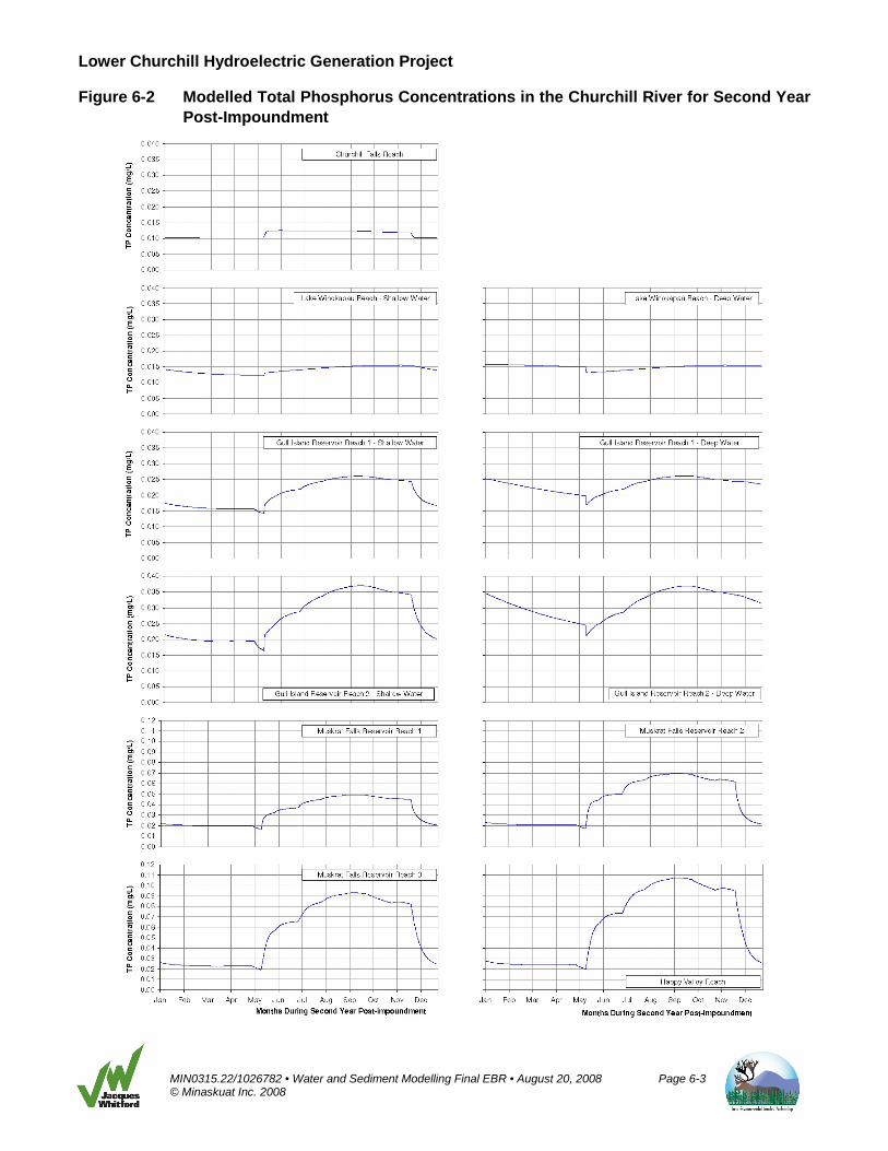
Lower Churchill Hydroelectric Generation Project
MIN0315.22/1026782 • Water and Sediment Modelling Final EBR • August 20, 2008 Page 6-3 © Minaskuat Inc. 2008
Figure 6-2 Modelled Total Phosphorus Concentrations in the Churchill River for Second Year Post-Impoundment
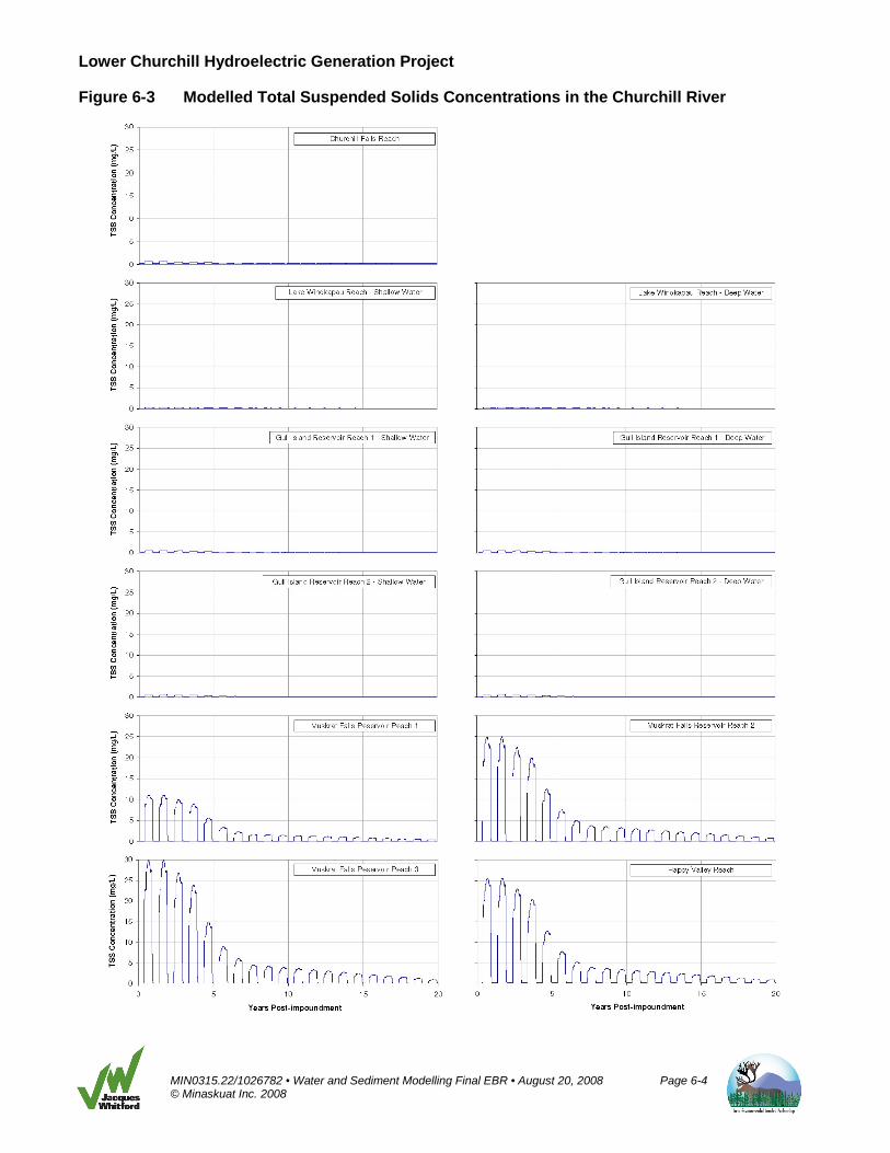
Lower Churchill Hydroelectric Generation Project
MIN0315.22/1026782 • Water and Sediment Modelling Final EBR • August 20, 2008 Page 6-4 © Minaskuat Inc. 2008
Figure 6-3 Modelled Total Suspended Solids Concentrations in the Churchill River

Lower Churchill Hydroelectric Generation Project
MIN0315.22/1026782 • Water and Sediment Modelling Final EBR • August 20, 2008 Page 6-5 © Minaskuat Inc. 2008
Figure 6-4 Annual Shoreline Erosion Intensity Over Time
0%
10%
20%
30%
40%
50%
60%
70%
80%
90%
100%
0 5 10 15 20
Ero
sio
n In
tens
ity
Years Post-Impoundment
Currently, the baseline concentration of TSS in the lower Churchill River are very low and typically below DLs (5 mg/L) (Minaskuat 2007a); baseline was assigned a value of 1 mg/L for modelling purposes. However, during the spring freshet, baseline concentrations may rise to between 11 and 127 mg/L, depending on the river reach, due to high turbulence and scouring of sediment in the streambed and river banks (Minaskuat 2007a). This is a typical cycle of TSS concentrations for rivers. After impoundment (with the exception of the Happy Valley reach below Muskrat Falls generating facility), unregulated runoff will continue to occur in the spring, but river levels will not rise as much as they did pre-impoundment, and water velocities within the impoundments will be lower. Therefore, the spring freshet spike in TSS concentrations will be weaker. Instead, in the impounded area, TSS concentrations will peak during summer due to shoreline erosion.
Predicted peak particulate concentrations were approximately one order of magnitude greater in reaches below Gull Island generating facility (ML1, ML2, ML3, and HV) than above it (Table 6-1). Greater erosion potential of the banks along this stretch of the river (AMEC 2007) was the main factor influencing these results. Beyond year 15, concentrations in all river reaches returned to levels approximating those of current baseline concentrations (Minaskuat 2007a) and will continue to fluctuate seasonally beyond the 20-year model (i.e., years 20 to 50).
Lower Churchill Hydroelectric Generation Project
MIN0315.22/1026782 • Water and Sediment Modelling Final EBR • August 20, 2008 Page 6-6 © Minaskuat Inc. 2008
Table 6-1 Peak Total Suspended Solids Concentration (mg/L) in Each River Reach
River Reach Maximum TSS Concentration (mg/L)
Churchill Falls Reach 0.65 Lake Winokapau Reach - Shallow Water 0.37 Lake Winokapau Reach - Deep Water 0.37 Gull Island Reservoir Reach 1 - Shallow Water 0.55 Gull Island Reservoir Reach 1 - Deep Water 0.55 Gull Island Reservoir Reach 2 - Shallow Water 0.52 Gull Island Reservoir Reach 2 - Deep Water 0.52 Muskrat Falls Reservoir Reach 1 11.08 Muskrat Falls Reservoir Reach 2 24.99 Muskrat Falls Reservoir Reach 3 29.95 Happy Valley Reach 25.65
6.2.2 Sensitivity Analysis for Total Suspended Solids
The sensitivity of the model was tested for six key parameters: Mixer and Dispers; Sediment Settling Velocity; River Flow; Kd; organic matter Decomposition Rate and Flooded Biomass. Only three of these variables would have effects on TSS concentrations. The Kd value and organic matter decomposition rate are applicable only to TP; therefore, their effects on TSS are not presented.
As expected, TSS concentrations in both reaches were sensitive to variation in Settling Velocity (Table 6-2). Varying the rate of mixing between deep and shallow cells (Mixer), and the rate of dispersion between deep cells (Dispers) only affected concentrations of TSS in the Gull Island reservoir when the rates were increased (Table 6-2). However, there was no effect on the Muskrat Falls reservoir, as there are no deep cells within this reach. Varying River Flow had little effect on TSS concentrations within the Gull Island reservoir, although a larger effect was observed within the Muskrat Falls reservoir. The effect of river flow on TSS in the Gull Island reservoir was opposite of that the Muskrat Falls reservoir, where increased river flow increased the TSS concentration in Gull Island reservoir, but decreased the TSS concentration in Muskrat Falls reservoir. This was because the background concentration of TSS was set at 1 mg/L and under reduced river flow, more TSS was able to settle out of the water column in the Gull Island reservoir. Because of the higher erosion potential of the banks along the Muskrat Falls reservoir (AMEC 2007), decreasing the river flow had the effect of increasing TSS concentrations there.

Lower Churchill Hydroelectric Generation Project
MIN0315.22/1026782 • Water and Sediment Modelling Final EBR • August 20, 2008 Page 6-7 © Minaskuat Inc. 2008
Table 6-2 Effect on Total Suspended Solids of Adjusting Sensitivity Analysis Parameters from Best-Case to Worst-Case
Parameter Effect on TSS
Gull Island Reservoir Muskrat Falls Reservoir Best-case
Best Estimate
Worst-case
Best-case
Best Estimate
Worst-case
Mixer and Dispers + 0.52 0.52 1.02 29.95 29.95 29.95 Settling Velocity - 0.35 0.52 0.71 24.67 29.95 34.10 River Flow +/-A 0.52 0.52 0.53 25.59 29.95 34.59 Combined Effect 0.34 - 5.98 21.40 - 39.71 A - river flow rate had a positive effect on TSS in Gull Island reservoir and a negative effect in the Muskrat Falls reservoir.
6.3 Long-term Phosphorus Projections
6.3.1 Best Estimate Scenario Results
Phosphorus concentrations exhibited a trend similar to that of TSS throughout the river. The TP concentration is expected to peak in the first year post-impoundment as a result of the greatest inputs from flooded and eroded soils and release from flooded biomass. Peak concentrations are expected to decrease rapidly in the decade following impoundment and less so thereafter (Figure 6-5).
This pattern is primarily the result of two processes occurring in tandem. As erosion decreases with time (Figure 6-4) due to the restabilization of the shoreline, there is less input of P from eroded soils into the water column. Likewise, as the flooded biomass decomposes, there is less biomass available to decompose and release P (Figure 6-6). These two combined processes result in the modelled pattern of TP within the reservoir.
Depending on the reach, current baseline concentrations of TP in the lower Churchill River range from 0.012 to 0.034 mg/L in the fall and 0.018 to 0.152 mg/L in the spring. Similar to the current pattern of TSS, concentrations of TP increase in the spring, but quickly return to lower summer levels (Minaskuat 2007a). The post-impoundment model projections indicate that concentrations will increase in the spring, though not to the same degree, but may persist through the ice-free period.
As with TSS, the highest TP concentrations are expected to occur in the sections of the river below the proposed Gull Island generating facility (i.e., in river reaches ML1, ML2, ML3 and HV), with the highest predicted concentration occurring in HV (best estimate = 0.115 mg/L; Table 6-3). Concentrations in this section of the river may increase by an order of magnitude above baseline concentrations (0.01 mg/L). However, by year 11, peak summer concentrations decreased to approximately 0.02 mg/L (Figure 6-5), concentrations that are similar to current annual peak concentrations in this river reach (Minaskuat 2007a). In fact, by year 11, all model reaches are projected to reach TP concentrations similar to current baseline concentrations measured from the respective river reach (Minaskuat 2007a), and continue to slowly decline to more stable background concentrations (years 20 to 50) due to greater dilution of spring freshet.
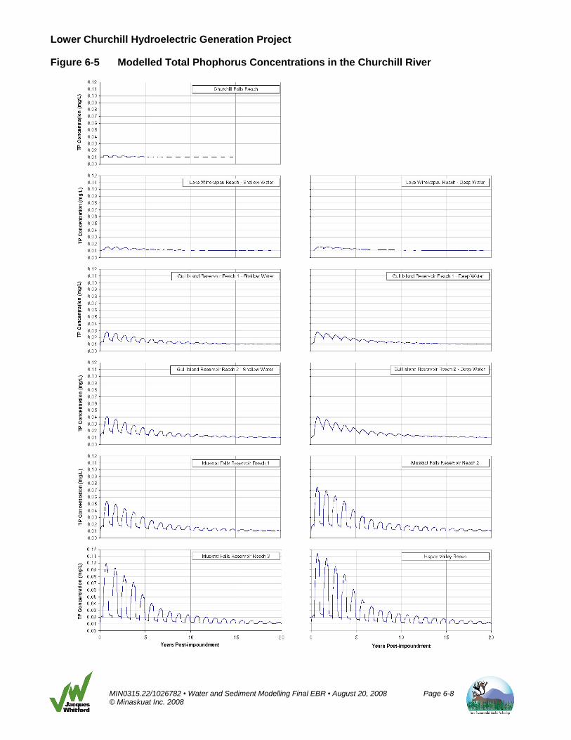
Lower Churchill Hydroelectric Generation Project
MIN0315.22/1026782 • Water and Sediment Modelling Final EBR • August 20, 2008 Page 6-8 © Minaskuat Inc. 2008
Figure 6-5 Modelled Total Phophorus Concentrations in the Churchill River

Lower Churchill Hydroelectric Generation Project
MIN0315.22/1026782 • Water and Sediment Modelling Final EBR • August 20, 2008 Page 6-9 © Minaskuat Inc. 2008
Figure 6-6 Percent Flooded Biomass Remaining in the Reservoir Over Time
0%
10%
20%
30%
40%
50%
60%
70%
80%
90%
100%
0 5 10 15 20
Rem
ain
ing
Bio
mas
s
Years Post-Impoundment
Table 6-3 Peak Total Phosphorus Concentrations in All River Reaches
Reach Maximum Phosphorus Concentration (mg/L)
Churchill Falls Reach 0.013 Lake Winokapau Reach - Shallow Water 0.016 Lake Winokapau Reach - Deep Water 0.016 Gull Island Reservoir Reach 1 - Shallow Water 0.028 Gull Island Reservoir Reach 1 - Deep Water 0.028 Gull Island Reservoir Reach 2 - Shallow Water 0.041 Gull Island Reservoir Reach 2 - Deep Water 0.041 Muskrat Falls Reservoir Reach 1 0.054 Muskrat Falls Reservoir Reach 2 0.075 Muskrat Falls Reservoir Reach 3 0.099 Happy Valley Reach 0.115
6.3.2 Sensitivity Analysis of Total Phosphorus
The sensitivity of TP concentration in the model was tested for all six key parameters. In Gull Island reservoir, TP concentrations were most sensitive to Decomposition Rate and River Flow, as well as clearing of Flooded Biomass. Settling Velocity, Mixer and Dispers, and Kd had negligible effects on TP concentrations (Table 6-4). In the Muskrat Falls reservoir, TP concentrations were most affected by a reduction in Flooded Biomass and variation in River Flow and Decomposition Rate. The three remaining parameters had relatively small influence (Table 6-4).
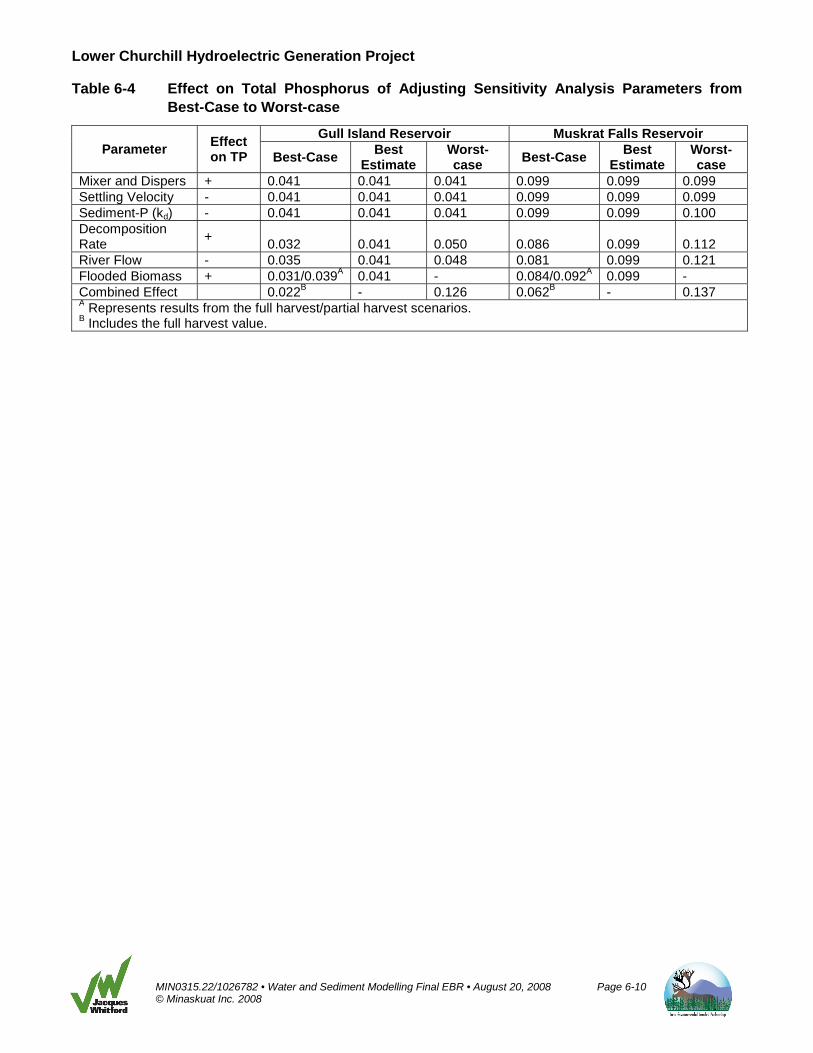
Lower Churchill Hydroelectric Generation Project
MIN0315.22/1026782 • Water and Sediment Modelling Final EBR • August 20, 2008 Page 6-10 © Minaskuat Inc. 2008
Table 6-4 Effect on Total Phosphorus of Adjusting Sensitivity Analysis Parameters from Best-Case to Worst-case
Parameter Effect on TP
Gull Island Reservoir Muskrat Falls Reservoir
Best-Case Best Estimate
Worst-case Best-Case Best
Estimate Worst-case
Mixer and Dispers + 0.041 0.041 0.041 0.099 0.099 0.099 Settling Velocity - 0.041 0.041 0.041 0.099 0.099 0.099 Sediment-P (kd) - 0.041 0.041 0.041 0.099 0.099 0.100 Decomposition Rate
+ 0.032 0.041 0.050 0.086 0.099 0.112
River Flow - 0.035 0.041 0.048 0.081 0.099 0.121 Flooded Biomass + 0.031/0.039A 0.041 - 0.084/0.092A 0.099 - Combined Effect 0.022B - 0.126 0.062B - 0.137 A Represents results from the full harvest/partial harvest scenarios. B Includes the full harvest value.

Lower Churchill Hydroelectric Generation Project
MIN0315.22/1026782 • Water and Sediment Modelling Final EBR • August 20, 2008 Page 7-1 © Minaskuat Inc. 2008
7.0 DISCUSSION
7.1 Projected Total Suspended Sediment Concentrations
Projected TSS concentrations in the Gull Island and Muskrat Falls reservoirs are expected to increase rapidly in the spring, remained elevated during the summer season, then decline during the ice-covered period as erosion ceases and suspended sediment settles or is flushed downriver. The first two years post-impoundment are projected to have the highest peak concentrations of TSS. Based on the model results and comparison with other reservoirs, peak TSS concentrations are expected to last approximately 5 to 10 years post-impoundment, after which TSS concentrations will gradually decline as the shorelines establish a new equilibrium. By the end of the 20-year model scenarios, concentrations approach equilibrium in all river reaches. Between 20 to 50 years, concentrations will continue to fluctuate seasonally and approximate current baseline concentrations with reduced peaks due to the sedimentation in reservoirs as a result of reduced turbulence caused by impoundment.
The best estimate scenario results in a peak TSS concentration of <1 mg/L in Gull Island reservoir and approximately 30 mg/L in Muskrat Falls reservoir. These concentrations are similar to those observed during baseline sampling at various stations located between Goose Bay and Churchill Falls in 2006 and 2007 as illustrated on Figure 1.1 (Minaskuat 2007a). The concentrations <1 mg/L in the reaches above the proposed Gull Island dam are a result of reduced river flow and turbulence due to impoundment and the low Erosion Potential of banks along these reaches. This is also due to the model initiating on January 1 of the year following impoundment, which begins as an ice-covered system, and does not account for unpredictable turbulence and processes that may occur during the flooding phase that may produce a short-term rise in TSS. The higher concentrations in the lower river reaches (i.e., below the proposed Gull Island dam) are a result of much higher Erosion Potential of the shorelines and the finer texture of the soils in these reaches (AMEC 2007). These latter concentrations are consistent with reported values for reservoirs throughout North America. In Missouri, 98 percent of 135 reservoirs surveyed had TSS concentrations below 30 mg/L (Jones and Knowlton 2005). TSS was modelled in Detroit Lake, Oregon, and the model was validated with real data (Sullivan et al. 2007). In that reservoir system, TSS increased from approximately 6 mg/L pre-impoundment to just above 25 mg/L post-impoundment.
Relatively few long-term monitoring data are available on post-impoundment reservoir TSS concentrations; however the model result trends are not unlike those of the Red Rock Reservoir in Iowa (DMRWQN 2007). Reservoir TSS concentrations in that system remained in the peak phase at very high concentrations for 12 to 15 years post-impoundment. The difference in concentrations duration is due to the sediment substrate being deep deposits of fine particulate and natural turbidity of the system. This results in a longer period of time for banks to restabilize and more frequent resuspension of sediments in that system.
Projected TSS concentrations from the lower Churchill River model are also consistent with observed TSS concentrations from several large Canadian river systems, indicating that these concentrations are not incompatible with healthy fish communities. In the MacKenzie River, Northwest Territories, TSS concentrations during average flow range from approximately 40 to 60 mg/L in the river delta (Emmerton 2006). These concentrations do not represent spring runoff, when TSS concentrations rise substantially. Similarly, in the Fraser River, British Columbia, TSS concentrations average 48 mg/L (ranging from 1 to 380 mg/L) near Hope, British Columbia (Swain et al. 1998).

Lower Churchill Hydroelectric Generation Project
MIN0315.22/1026782 • Water and Sediment Modelling Final EBR • August 20, 2008 Page 7-2 © Minaskuat Inc. 2008
7.2 Projected Total Phosphorus Concentrations
The projected concentration of TP over the 20-year projection begins with a substantial increase, followed by a five- to six-year period of rapid decline and a 10- to 15-year period of restabilization. During winter periods where there is less input from shoreline erosion and vegetation decomposition, the majority of the suspended TP and particulate in the Churchill River are flushed downriver. Beyond the 20-year modelling projection (years 20 to 50), concentrations of TP will remain near current baseline concentrations (Minaskuat 2007a), but will reach a more stable equilibrium due to the dilution effect of reservoirs to the input of P from the spring freshet.
In the model reaches between Churchill Falls and the proposed Gull Island generating facility, concentrations of TP in both the shallow water and deep water are expected to increase to between 0.013 and 0.041 mg/L, an approximately four-fold increase from the typical background concentration of 0.01 mg/L. According to the CCME (2004) trophic categories for Lakes and Rivers in Canada, these reaches would change from being oligotrophic to mesotrophic or meso-eutrophic. A trophic shift may not be fully realized due to the rapid flushing rate of the reservoir.
In the three model reaches of the Muskrat Falls reservoir, and in the Happy Valley reach, TP concentrations of between 0.054 and 0.115 mg/L are predicted; all peak concentrations in these stretches would fall into the eutrophic or hyper-eutrophic categories according to CCME rankings, although again, these trophic shifts might not be fully realized due to rapid flushing and shading caused by elevated TSS concentrations. While these peak concentrations represent substantial increases above background concentrations, they remain within the range that would result in increased fish production and below concentrations where summer kill due to anoxia from algal blooms would likely occur (Stockner et al. 2000, Jeppesen et al. 2005). Furthermore, modelled peak TP concentrations are within the range of current TP concentrations observed during 2006 and 2007 (Figure 1.2; Minaskuat 2007a).
Primary productivity in the Churchill River would likely be lower than the potential during the early period (0 to 10 years) post-impoundment based on nutrient levels in the reservoir (Stockner et al. 2001). Productivity below potential in that reservoir system has been attributed to the reduced light transmission from the increased suspended sediment load in the reservoir. Given that the peak TP and TSS concentrations are projected to occur over a similar temporal scale, the antagonistic interaction of these two parameters on primary productivity and the flushing effect of river flow would serve to mitigate water quality issues related to eutrophication in the early periods post-impoundment (0 to 10 years).
It was assumed that due to turbulence and water temperatures, oxygenated water would circulate through all flooded areas of the reservoirs. If some deep portions were to become anoxic, decomposition rates would be lower in those portions, which would result in a lower input of phosphorus into the system over a longer period of time.
7.3 Model Sensitivity Analysis
The sensitivity of the model to variation in six key parameters (Mixer and Dispers, Settling Velocity, Sediment-P (Kd), Decomposition Rate, River Flow and Flooded Biomass) was tested. In addition to the best estimate value (default value), a low and high value based on reported values in the literature and
Lower Churchill Hydroelectric Generation Project
MIN0315.22/1026782 • Water and Sediment Modelling Final EBR • August 20, 2008 Page 7-3 © Minaskuat Inc. 2008
professional judgement were assigned. The observed model sensitivity to variation in the key model variables and the potential implications for these are discussed in this section.
In the Gull Island reservoir, TSS concentrations were most sensitive to Settling Velocity and an increase in Mixer and Dispers. Being a large reservoir, with deep water compartments and surface drawdown, the Gull Island reservoir will be an effective sediment trap. Thus, increasing Settling Velocity will allow greater quantities of particulates to be deposited into bottom sediments. Suspended sediment concentrations were sensitive to Mixer and Dispers because increases in these values influenced the rate of exchange among cells particularly the shallow and deep water cells of Gull Island reservoir. Variation in River Flow had very little effect on TSS in Gull Island reservoir, due to the fact that erosion rates in this reservoir will remain quite low, and the background TSS concentration is quite low.
In the Muskrat Falls reservoir, TSS concentrations were equally sensitive to Settling Velocity and River Flow. Variation in Settling Velocity influenced the quantity of particulate settling into bottom sediment, as was the case in Gull Island reservoir, but there is no deep water compartment in Muskrat Falls reservoir, and this reservoir will have bottom drawdown. Increasing River Flow resulted in lower TSS concentrations due to dilution with relatively low TSS water from the Gull Island reservoir.
In the Gull Island reservoir, TP concentrations were most sensitive to Decomposition Rate and River Flow and a decrease in Flooded Biomass from harvesting and clearing. This was as expected since biomass decomposition represents a major input of TP, and increasing Decomposition Rate would result in a more rapid initial input and a faster return to equilibrium. Altering River Flow influenced residency time within the reservoir and affected the ability of TP to accumulate in the lakes. As would be expected, a decrease in the amount of Flooded Biomass decreased the amount of TP because less biomass was present to decompose and release P into the water column. The TP was relative insensitive to Settling Velocity or Sediment-P (kd). Most P is present in dissolved form; Settling Velocity only affects suspended sediment. Therefore altering this parameter only affected the small fraction of TP bound to suspended sediment. In Muskrat Falls reservoir, TP concentrations were most sensitive to River Flow, Decomposition Rate and a decrease in flooded biomass, similar to results from Gull Island reservoir, and less sensitive to Settling Velocity and Sediment-P (kd).
Overall, the model sensitivity analysis indicates that the model has relatively low sensitivity to most of the parameter values, and that overall confidence in the best estimate values can be quite high. The range in projected TSS concentrations between best-case and worst-case estimates was relatively small (0.34 to 5.98 mg/L in the Gull Island reservoir, and 21.40 to 39.71 mg/L in the Muskrat Falls reservoir). Concentrations of TP (0.022 to 0.126 mg/L in the Gull Island reservoir, and 0.062 to 0.137 in the Muskrat Falls reservoir) had similar relative variability to TSS. These ranges can be considered confidence intervals for the best estimate values.
7.4 Model Uncertainties
7.4.1 Erosion rates
Shoreline erosion rates and data provided by AMEC (2007) were used in the TSS and TP models. The sensitivity of the models to this parameter was not tested because these were considered to be worst-case values.
Lower Churchill Hydroelectric Generation Project
MIN0315.22/1026782 • Water and Sediment Modelling Final EBR • August 20, 2008 Page 7-4 © Minaskuat Inc. 2008
7.4.2 Spatial Sediment Distribution
The model assumes that sediment inputs into the reservoir will be instantaneously distributed in a homogeneous manner throughout the model cell. However, this is unlikely to occur. Realistically, there will be higher concentrations of TSS and TP in areas proximal to eroding shorelines, while areas further removed from the sediment and nutrient inputs will have lower concentrations. The mass balance model approach can not readily quantify the magnitude of these heterogeneities; however, it is typically accepted that the sediment-water or shoreline-water interfaces have higher TSS and TP concentrations than open water (Roberts 2004).
7.5 Summary and Conclusions
The objective of this study was to develop a conceptual water quality model structure for the lower Churchill River (i.e., that portion of the Churchill River system in Labrador that lies between the tailrace of the existing Smallwood Reservoir, and the mouth of the river near Happy-Valley Goose Bay, Labrador), as it will be post-impoundment, and to implement the model using the STELLA® modelling software system, to provide models to estimate TSS and TP concentrations in the water for a 50-year period following impoundment.
Based on the model projections, TSS and TP concentrations will remain at relatively low levels in the Gull Island reservoir, but will increase substantially (TSS - 12 to 30 mg/L; TP – 0.013 to 0.115 mg/L) for a number of years post-impoundment in the Muskrat Falls reservoir. These results are due primarily to the greater shoreline erosion potential of these reaches. The peak concentrations of both TSS and TP in all reaches are expected to decline within 5 to 10 years post-impoundment as shoreline erosion rates decrease and after most flooded biomass has decomposed. Several river systems throughout Canada have healthy fish populations despite natural TSS concentrations exceeding projections of this study.
Projected peak TSS concentrations ranged from <1 to approximately 30 mg/L in the various modelled reaches of the river, and occurred during the first year post-impoundment. However, by the end of the 20-year modelling projection, concentrations in all reaches were below 2 mg/L. According to CCME (1999) guidelines, long-term increases in TSS should not exceed 5 mg/L above baseline. While the projected mean concentrations remain below the maximum concentration reported from the baseline study (127 mg/L), TSS concentrations through most of the open water season will be higher than baseline concentrations during the first 10 years post-impoundment.
Projected TP concentrations of the river system rose to between 0.013 and 0.115 mg/L; nutrient inputs to the river post-impoundment will likely raise the trophic state. However, primary production is unlikely to increase to maximum potential due to flow through and the counteractive effect of shading caused by increased TSS concentrations, which occur simultaneously. Full removal of above-ground vegetation (Full Clearing scenario; see Section 6.3.2) resulted in a TP concentration of 0.84 mg/L in the Muskrat Falls reservoir, a reduction of 0.15 mg/L from 0.99 mg/L using the best-estimate (no clearing) scenario. As biomass removal will likely fall somewhere between these extremes, actual concentrations are likely to be between 0.99 and 0.84 mg/L in this reach. Due to reservoir clearing, a similar relative difference can be expected in the other reaches as well.
The sensitivity of the model to six key parameters was tested. Model sensitivity was greatest to variations in river flow, vegetation decomposition and sediment particle settling rates. When all sensitivity analysis parameters were set to values that produced the highest (worst-case)

Lower Churchill Hydroelectric Generation Project
MIN0315.22/1026782 • Water and Sediment Modelling Final EBR • August 20, 2008 Page 7-5 © Minaskuat Inc. 2008
concentrations of TSS and TP, peak TSS and TP concentrations in the first year post-impoundment increased by approximately 9.76 mg/L and 0.038 mg/L, respectively, above best estimate levels in the Muskrat Falls reservoir, where the highest concentrations in the river were observed from the best estimate scenario.

Lower Churchill Hydroelectric Generation Project
MIN0315.22/1026782 • Water and Sediment Modelling Final EBR • August 20, 2008 Page 8-1 © Minaskuat Inc. 2008
8.0 CLOSURE
This report has been prepared for the sole benefit of Newfoundland and Labrador Hydro. The report may not be used by any other person or entity, other than for its intended purposes, without the consent of Minaskuat and Newfoundland and Labrador Hydro.
The information and conclusions contained in this report are based upon work undertaken in accordance with generally accepted engineering and scientific practices current at the time the work was performed. The information provided in this report was compiled from existing documents, design information provided by Newfoundland and Labrador Hydro, data provided by regulatory agencies and others. Information obtained from secondary sources has been assumed to be correct; Minaskuat accepts no responsibility for damages or liability that may arise from use of this data.
If any conditions become apparent that differ significantly from our understanding of conditions as presented in this report, Minaskuat requests that we be notified immediately, and permitted to reassess the conclusions provided herein.
This report was prepared by Jean-Michel DeVink, Ph.D., and Paul Mazzocco, B.Sc., and was Senior Reviewed by Malcolm Stephenson, Ph.D.
MINASKUAT LIMITED PARTNERSHIP
(Final to be signed by) (Final to be signed by) Jean-Michel DeVink, Ph.D. Environmental Scientist
Malcolm Stephenson, Ph.D. Principal Study Manager, Senior Technical Review
Lower Churchill Hydroelectric Generation Project
MIN0315.22/1026782 • Water and Sediment Modelling Final EBR • August 20, 2008 Page 9-1 © Minaskuat Inc. 2008
9.0 REFERENCES
9.1 Literature Cited
AMEC Earth and Environmental. 2007. Bank Stability Study: Proposed Lower Churchill River Hydroelectric Development, Labrador. Draft report TF6110449 prepared for Newfoundland and Labrador Hydro, St. John’s, NL.
Carignan, R. and D.R.S. Lean. 1991. Regeneration of dissolved substances in a seasonally anoxic lake: the relative importance of processes occurring in the water column and in the sediments. Limnology and Oceanography 36: 683-707.
CCME (Canadian Council of Ministers of the Environment). 1999. Canadian Water Quality Guidelines for the Protection of Aquatic Life: Total Particulate Matter. Factsheet, updated in 2002.
CCME (Canadian Council of Ministers of the Environment). 2004. Canadian Water Quality Guidelines for the Protection of Aquatic Life: Phosphorus. Factsheet.
Diamond, M.L., D. Mackay, D.J. Poulton and F.A. Stride. 1994. Development of a mass balance model of the fate of 17 chemicals in the Bay of Quinte. Journal of Great Lakes Research 20: 643-666.
Diamond, M.L., D. Mackay, D.J. Poulton, and F.A. Stride. 1996. Assessing the chemical behaviour and developing remedial actions using a mass balance model of chemical fate in the Bay of Quinte. Water Research 30: 405-421.
Elçi, , P.A. Work and E.J. Hayter. 2007. Influence of stratification and shoreline erosion on reservoir sedimentation patterns. Journal of Hydrological Engineering 133: 255-266.
Emmerton, C.A. 2006. Downstream Nutrient Changes Through the Mackenzie River Delta and Estuary, Western Canadian Arctic. M.Sc. Thesis. Simon Fraser University, Burnaby, BC.
EnFor Consulting Services. 2008. Lower Churchill River Power Project Reservoir Preparation Plan – Update 2007. Draft Report. Volume I – Preparation Plan and Cost Estimate.
Froelich, P.N. 1988. Kinetic control of dissolved phosphate in natural rivers and estuaries: a primer on the phosphate buffer mechanism. Limnology and Oceanography 33: 649-668.
GESAMP (IMA/FAO/ UNESCO/WMO/WHO/IAEA/UN/UNEP Joint Group of Experts on the Scientific Aspects of Marine Pollution). 1991. Coastal Modeling. GESAMP Reports and Studies No. 43, 192 pp.
Hall, R.I., P.R. Leavitt, A.S. Dixit, R. Quinlan and J.P. Smol. 1999. Limnological succession in reservoirs: a paleolimnological comparison of two methods of reservoir formation. Canadian Journal of Fisheries and Aquatic Sciences 56:1109-1121.
Hatch. 2007. Ice Dynamics of the Lower Churchill River. Draft report prepared for Newfoundland and Labrador Hydro, St. John’s, NL.
Hill, P.S., T.G. Milligan, and W.R. Geyer. 2000. Controls on effective settling velocity of suspended sediment in the Eel River flood plume. Continental Shelf Research 20: 2095-2111.
House, W.A. 2003. Geochemical cycling of phosphorus in rivers. Applied Geochemistry 18: 739-748.
Lower Churchill Hydroelectric Generation Project
MIN0315.22/1026782 • Water and Sediment Modelling Final EBR • August 20, 2008 Page 9-2 © Minaskuat Inc. 2008
Jeppesen, E., M. Søndergaard, J.P. Jensen, K.E. Havens, O. Anneville, L. Carvalho, M.F. Coveney, R. Deneke, M.T. Dokulil, B. Foy, D. Gerdeaux, S.E. Hampton, S. Hilt, K. Kangur, J. Köhler, E.H.H.R. Lammens, T.L. Lauridsen, M. Manca, M.R. Miracle, B. Moss, P, Nõges, G. Persson, G. Phillips, R. Porteilje, S. Romo, C. L. Schelske, D. Straile, I. Tatrai, E. Willén and M. Winder. 2005. Lake reseponses to reduced nutrient loading - An analysis of contemporary long-term data from 35 case studies. Freshwater Biology 50: 1747-1771.
JWEL (Jacques Whitford Environment Limited). 1999. 1998 Water and Sediment Quality of the Churchill River (LHP 98-08). Newfoundland and Labrador Hydro, St. John’s, NL.
Jones, J.R. and M.F. Knowlton. 2005. Suspended solids in Missouri reservoirs in relation to catchment features and internal processes. Water Research 39: 3629-3635.
Kennedy, R.H. and W.W. Walker. 1990. Reservoir nutrient dynamics. Pp. 109-132. In: K.W. Thornton, B.L. Kimmel, and F.E. Payne (eds.). Reservoir Limnology: Ecological Perspectives. John Wiley & Sons, New York.
Kerr, S.J. 1995. Silt, turbidity, and suspended sediments in the aquatic environment: an annotated bibliography and literature review. Ontario Ministry of Natural Resources, Southern Region Science and Technology Transfer Unit Technical Report TR-008: 277 pp.
Kimmel, B.L., O.T. Lind and L.J. Paulson. 1990. Reservoir primary production. Pp. 133-194. In: K.W. Thornton, B.L. Kimmel and F.E. Payne (eds.). Reservoir Limnology: Ecological Perspectives. John Wiley & Sons, New York.
Larmola, T., J. Alm, S. Juutinen, D. Koppisch, J. Augustin, P.J. Martikainen and J. Silvola. 2006. Spatial patterns of litter decomposition in the littoral zone of boreal lakes. Freshwater Biology 51: 2252-2264.
Li, Z., W.A. Kurz, M.J. Apps and S.J. Beukema. 2003. Belowground biomass dynamics in the Carbon Budget Model of the Canadian Forest Sector: recent improvements and implications for the estimation of NPP and NEP. Canadian Journal of Forest Research 33: 126-136.
Lorang. M.S. and J.A. Stanford. 1993. Variability of shoreline erosion and accretion within a beach compartment of Flathead Lake, Montana. Limnology and Oceanography 38: 1783-1795.
Minaskuat Inc.. 2007a. Water and Sediment Quality in the Churchill River Environmental Baseline Report LHP 06-04. Report prepared for Newfoundland and Labrador Hydro, St. John’s, NL.
Minaskuat Limited Partnership. 2007b. Project Area Ecological Land Classification Environmental Baseline Report. Interim Report prepared for Newfoundland and Labrador Hydro, St. John’s, NL.
Moore, T.R., J.L. Bubier, S.E. Frolking, P.M. LaFleur and N.T. Roulet. 2002. Plant biomass and production and CO2 exchange in an ombrotrophic bog. Journal of Ecology 90: 25-36.
Newbury, R.W., and G.K. McCullough. 1984. Shoreline erosion and restabilization in the Southern Indian Lake reservoir. Canadian Journal of Fisheries and Aquatic Science 41: 558-566.
Newcombe, C.P. 1994. Suspended Sediment Pollution: Dose Response Characteristics of Various Fishes. Draft Report, Habitat Protection Branch, British Columbia Ministry of Environment, Lands and Parks, Victoria, BC. 45 pp.
Lower Churchill Hydroelectric Generation Project
MIN0315.22/1026782 • Water and Sediment Modelling Final EBR • August 20, 2008 Page 9-3 © Minaskuat Inc. 2008
Onishi, Y., R.J. Serne, E.M. Arnold, C.E. Cowan and F.L. Thompson. 1981. Critical Review: radionuclide transport, sediment transport, and water quality mathematical modeling; and radionuclide adsorption/desorption mechanisms. Report Prepared for U.S. Nuclear Regulatory Commission, NUREG/CR-1322.
Pant, H.K. and K.R. Reddy. 2001. Phosphorus sorption characteristics of estuarine sediments under different redox conditions. Journal of Environmental Quality 30: 1474-1480.
Prescott, C.E., L. Vesterdal, C.M. Preston and S.W. Simard. 2004. Influence of initial chemistry on decomposition of foliar litter in contrasting forest types in British Columbia. Canadian Journal of Forest Research 34: 1714-1729.
Ragozin, A.L. and V.N. Burova. 1993. Method of quick predictive estimate of the rate of reworking reservoir banks. Hydrotechnical Construction 27:577-585.
Reichstein, M., J.-A. Subke, A.C. Angeli and J.D. Tenhunen. 2005. Does the temperature sensitivity of decomposition of soil organic matter depend upon water content, soil horizon, or incubation time? Global Change Biology 11: 1754-1767.
Rejmánková, E. and K. Houdková. 2006. Wetland plant decomposition under different nutrient conditions: what is more important, litter quality or site quality? Biogeochemistry 80: 245-262.
Roberts, K.L. 2004. Modeling of River Hydrodynamics and Active Cap Effectiveness in the Anacostia River. MSc Thesis. Louisiana State University, Baton Rouge, LA.
Saint-Laurent, D., B.N. Touileb. J.-P. Saucet, A. Whalen, B. Gagnon and T. Nzakinuena. 2001. Effects of simulated water level management on shore erosion rates. Case study: Baskatong Reservoir, Quebec, Canada. Canadian Journal of Civil Engineering 28: 482-495.
Soetaert, K. and P.M.J. Herman. 1995a. Estimating estuarine residence times in the Westerschelde (The Netherlands) using a box model with fixed dispersion coefficients. Hydrobiologia 311: 215-224.
Soetaert, K. and P.M.J. Herman. 1995b. Carbon flows in the Westerschelde Estuary (The Netherlands) evaluated by means of an ecosystem model (MOSES). Hydrobiologia 311: 247-266.
Stephenson, M., J.A.K. Reid, Y. Zhuang and S.B. Russell. 1995. Preliminary assessment of low- and intermediate-level waste disposal in the Michigan Basin: large lake model. Atomic Energy of Canada Limited Report, COG-95-256.
Stockner, J.G., A.R. Langston and G.A. Wilson. 2001. The limnology of Williston Reservoir. Peace/Williston Fish and Wildlife Compensation Program 242. 51 pp.
Stockner, J.G., R. Rydin and P. Hyenstrand. 2000. Cultural oligotrophication: causes and consequences for fisheries resources. Fisheries 25: 7-14.
Sullivan, A.B., S.A. Rounds, S. Sobieszczyk and H.M. Bragg. 2007. Modeling Hydrodynamics, Water Temperature, and Suspended Sediment in Detroit Lake, Oregon. US Department of the Interior, US Geological Survey, Scientific Investigations Report 2007-5008.
Sundareshwar, P.V. and J.T. Morris. 1999. Phosphorus sorption characteristics of intertidal marsh sediments along an estuarine salinity gradient. Limnology and Oceanography 44: 1693-1701.
Lower Churchill Hydroelectric Generation Project
MIN0315.22/1026782 • Water and Sediment Modelling Final EBR • August 20, 2008 Page 9-4 © Minaskuat Inc. 2008
Swain, L.G., D.G. Walton, B. Phippen, H. Lewis, S. Brown, G. Bamford, D. Newsom and I. Lundman. 1998. Water Quality Assessment and Objectives for the Fraser River from Hope to Sturgeon and Robertson Banks. Ministry of Environment, Lands and Parks, BC. First Update, Technical Appendix.
Thompson, C.C., A.D. McGuire, J.S. Clein F.S. Chapin III and J. Beringer. 2005. Net carbon exchange across the Arctic tundra-boreal forest transition in Alaska 1981-2000. Mitigation and Adaption Strategies for Global Change 11: 805-827.
USEPA (United States Environmental Protection Agency). 1985. Rates, constants, and kinetics formulations in surface water quality modeling (Second Edition). EPA/600/3-85/040.
USEPA (United States Environmental Protection Agency). 1987. Processes, coefficients, and models for simulating toxic organics and heavy metals on surface waters. EPA/600/3-87/015
Westrich, J.T. and R.A. Berner. 1984. The role of sedimentary organic matter in bacterial sulfate reduction: the G model tested. Limnology and Oceanography 29: 236-249.
9.2 Internet Sites
DMRWQN (Des Moines River Water Quality Network). 2007. Downloadable Project Data. Available at: http://te-webserver.cce.iastate.edu/research/lutz/dmrwqn/dmrwqn.html (accessed 01/04/2008)
Millero, F.J. and J.-Z. Zhang. 2000. The Role of Suspended Calcium Carbonate in the Phosphorus Cycle in Florida Bay. NOAA COP Project Final Report. Available at: http://www.aoml.noaa.gov/ocd/sferpm/millero/millero_final.html (accessed, 11/27/2007)
Lower Churchill Hydroelectric Generation Project
MIN0315.22/1026782 • Water and Sediment Modelling Final EBR • August 20, 2008 Page 10-1 © Minaskuat Inc. 2008
10.0 ACRONYM LIST Acronym/ Symbol Definition
< A mathematical symbol meaning less than.
> A mathematical symbol meaning greater than.
A mathematical symbol representing less than or equal to.
A mathematical symbol representing greater than or equal to.
°C Degrees Celsius; a measurement of temperature.
µm Micromoles; a measurement of amount of substance
asl above sea level
CCME Canadian Council of Ministers of the Environment
Con Concentration
d Day; a measurement of time.
DS downstream
e.g., for example
EC Environment Canada
ELC Ecological Land Classification
EOSD Earth Observation for Sustainable Development
et al. and others
g Grams; a measurement of mass.
HV Happy Valley
Hydro Newfoundland and Labrador Hydro
i.e., that is to say, in other words
k Decomposition rate
Kd Water/sediment partitioning coefficient
kg Kilograms; a measurement of mass.
km Kilometres; a measurement of distance.
km2 Kilometres squared, a measurement of area.
kV Kilovolt
L Litres; a measurement of fluid volume.
m Metres; a measurement of distance.
m2 Metres squared; a measurement of area.
m3 Metres cubed; a measurement of volume.
m3/kg Metres cubed per kilogram; a measurement of distance over mass.
m3/s Metres cubed per second; a measurement of distance over time
mg Milligrams; a measurement of mass
mg/L Milligrams per litre; a measurement of mass over volume.
MW Megawatt
NTS National Topographic System
P Phosphorus
Lower Churchill Hydroelectric Generation Project
MIN0315.22/1026782 • Water and Sediment Modelling Final EBR • August 20, 2008 Page 10-2 © Minaskuat Inc. 2008
Acronym/ Symbol Definition
The Project Lower Churchill Hydroelectric generation Project
Q10 effect Rate of change of biochemical processes with a change of 10oC in temperature
RDL Reportable levels of detection.
s Seconds; a measurement of time.
TP Total Phosphorus
TSS Total Suspended Solids
US upstream
USEPA United States Environmental Protection Agency
Vol volume
yr Year; a measurement of time.


Lower Churchill Hydroelectric Generation Project Appendix A - The STELLA® Model Equations
Appendix A
The STELLA® Model Equations


CFc(t) = CFc(t - dt) + (USc:CFc + Erosion_CFc - CFc:WSc - CFc:CFMc) * dtINIT CFc = 0
DOCUMENT: CFc - Chuchill Falls reach, clay compartment. This extends from km 284 to km 334 (the tail race of the existing Churchill Falls project), and is modelled as a fully mixed water body. The compartment records the mass of clay (g) in the water.
INFLOWS:USc:CFc = TSS_Conc_Clay*Churchill_Falls_Flow_cDOCUMENT: Mass of TSS entering CHS from US is equal to the seasonally adjusted TSS concentration (kg/m3) in US water multiplied by the seasonally adjusted volume of water discharged at Churchill Falls (m3/d).
Erosion_CFc = (Ice_c * (856*1650000/196) * Erosion_Intensity) + ((Unregulated_Runoff_c * 2181354075.207)*TSS_Conc_Clay)DOCUMENT: Amount of Clay (g/day) entering CF weighted for ice free times of the year
1650000 is the density of silt in g/m3196 = ice free days856 = Eroded Volume of Clay (m3)2181354075.207 = Unregulated Segment Drainage Area (m2)
OUTFLOWS:CFc:WSc = CFc*(((Unregulated_Runoff_c * 2174263646) + Churchill_Falls_Flow_c)/Vol_CF)DOCUMENT: Mass of TSS entering WS from CF is equal to the mass in CF multiplied by the fractional replacement of water in CF.
Total water moving through this reach is the sum of water entering from the regulated Churchill Falls flow plus the cumulative unregulated flow. This is calculated as the cumulative watershed area of unregulated drainage into the CF segment (m2) times the seasonally adjusted unregulated runoff (m/d)
CFc:CFMc = CFc*Clay_SedRate/(Vol_CF/Area_CF)DOCUMENT: Mass transfer (g/day) from water to sediments.
CFMc(t) = CFMc(t - dt) + (CFc:CFMc) * dtINIT CFMc = 0
DOCUMENT: CFMc - Chuchill Falls reach, clay in mud compartment. The compartment records the mass of clay in sediments (g).
INFLOWS:CFc:CFMc = CFc*Clay_SedRate/(Vol_CF/Area_CF)DOCUMENT: Mass transfer (g/day) from water to sediments.

CFMp(t) = CFMp(t - dt) + (CFp:CFMp) * dtINIT CFMp = 0
DOCUMENT: CFMp - Chuchill Falls reach, phosphorus in mud compartment. The compartment records the mass of phosphorus in sediments (g).
INFLOWS:CFp:CFMp = (CFp*((Kd*Con_CFc)/(1+Kd*Con_CFc))*(SedRate_p/(Vol_CF/Area_CF)))DOCUMENT: Mass transfer (g/day) from water to sediments.
CFMs(t) = CFMs(t - dt) + (CFs:CFMs) * dtINIT CFMs = 0
DOCUMENT: CFMs - Chuchill Falls reach, silt in mud compartment. The compartment records the mass of silt in sediments (g).
INFLOWS:CFs:CFMs = CFs*Silt_SedRate/(Vol_CF/Area_CF)DOCUMENT: Mass transfer (g/day) from water to sediments.
CFp(t) = CFp(t - dt) + (USp:CFp + Erosion_CFp - CFp:WSp - CFp:CFMp) * dtINIT CFp = 0.01*241468601
DOCUMENT: CFp - mass (g) of phosphorus in Churchill Falls reach water compartment. This extends from km 284 to km 334 (the tail race of the existing Churchill Falls project), and is modelled as a fully mixed water body.
INFLOWS:USp:CFp = Baseline_P*Churchill_Falls_Flow_pDOCUMENT: Mass of TSPhosphorous S entering CHS from US is equal to the seasonally adjusted TSS concentration (kg/m3) in US water multiplied by the seasonally adjusted volume of water discharged at Churchill Falls (m3/d).

Erosion_CFp = (Ice_p * (16131*1000/196) * Erosion_Intensity_p) + ((Unregulated_Runoff_p * 2181354075.207)*Baseline_P)+ (Daily_P_Loss * 4038066)DOCUMENT: Amount of Phosphorous (g/day) entering CF from shoreline erosion and decomposion of organic matter in flooded soils and vegetation, adjusted for frozen or ice free times of the year.
1000 = g/kg conversion factor196 = ice free days16131 = Eroded Volume of Phosphorous (kg)2181354075.207 = Unregulated Segment Drainage Area (m2)4038066 = Flooded Segment Area (m2)
OUTFLOWS:CFp:WSp = CFp*(((Unregulated_Runoff_p * 2174263646) + Churchill_Falls_Flow_p)/Vol_CF)DOCUMENT: Mass of Phosphorous entering WS from CF is equal to the mass in CF multiplied by the fractional replacement of water in CF.
Total water moving through this reach is the sum of water entering from the regulated Churchill Falls flow plus the cumulative unregulated flow. This is calculated as the cumulative watershed area of unregulated drainage into the CF segment (m2) times the seasonally adjusted unregulated runoff (m/d)
CFp:CFMp = (CFp*((Kd*Con_CFc)/(1+Kd*Con_CFc))*(SedRate_p/(Vol_CF/Area_CF)))DOCUMENT: Mass transfer (g/day) from water to sediments.
CFs(t) = CFs(t - dt) + (USs:CFs + Erosion_CFs - CFs:WSs - CFs:CFMs) * dtINIT CFs = 0
DOCUMENT: CFs - Chuchill Falls reach, mass (g) of silt in water compartment. This extends from km 284 to km 334 (the tail race of the existing Churchill Falls project), and is modelled as a fully mixed water body.
INFLOWS:USs:CFs = TSS_Conc_Silt*Churchill_Falls_Flow_sDOCUMENT: Mass of TSS entering CHS from US is equal to the seasonally adjusted TSS concentration (kg/m3) in US water multiplied by the seasonally adjusted volume of water discharged at Churchill Falls (m3/d).

Erosion_CFs = (Ice_s * (25273*1650000/196) * Erosion_Intensity) + ((Unregulated_Runoff_s * 2181354075.207)*TSS_Conc_Silt)DOCUMENT: Amount of Silt (g/day) entering CF weighted for ice free times of the year
1650000 is the density of silt in g/m3196 = ice free days25273 = Eroded Volume of Silt (m3)2181354075.207 = Unregulated Segment Drainage Area (m2)
OUTFLOWS:CFs:WSs = CFs*(((Unregulated_Runoff_s * 2174263646) + Churchill_Falls_Flow_s)/Vol_CF)DOCUMENT: Mass of TSS entering WS from CF is equal to the mass in CF multiplied by the fractional replacement of water in CF.
Total water moving through this reach is the sum of water entering from the regulated Churchill Falls flow plus the cumulative unregulated flow. This is calculated as the cumulative watershed area of unregulated drainage into the CF segment (m2) times the seasonally adjusted unregulated runoff (m/d)
CFs:CFMs = CFs*Silt_SedRate/(Vol_CF/Area_CF)DOCUMENT: Mass transfer (g/day) from water to sediments.
C_stock(t) = C_stock(t - dt) + (- Decay_C) * dtINIT C_stock = 1
DOCUMENT: C_stock - this is used to help calculate the release rate of P from sediments, via the decomposition of organic matter (carbon). The initial mass of carbon in sediments is assumed to be 1 unit, and the daily loss as a fraction of the initial total quantity is modeled through Decay C.
OUTFLOWS:Decay_C = ((C_stock * ((Ice_p*0.3*Decaymaster/365) + ((Ice_p-1)*(-1)*0.074*Decaymaster/365))))DOCUMENT: Decay_C - this flow estimates the daily fraction of carbon that decomposes from an initial unit quantity. The variable Ice_p determines whether it is summer (Ice_p = 1) or winter (Ice_p = 0), and the carbon decomposition rate is adjusted from a summer value of 0.3/year to a winter value of 0.074/year. The ratio of 0.3 to 0.074 is based on an assumed summer temperature of 15C and winter temperature of 0C, and the assumption that based on Q10 theory and measurements, microbial activity decreases by a factor of 2.7 with a temperature decrease of 10C.
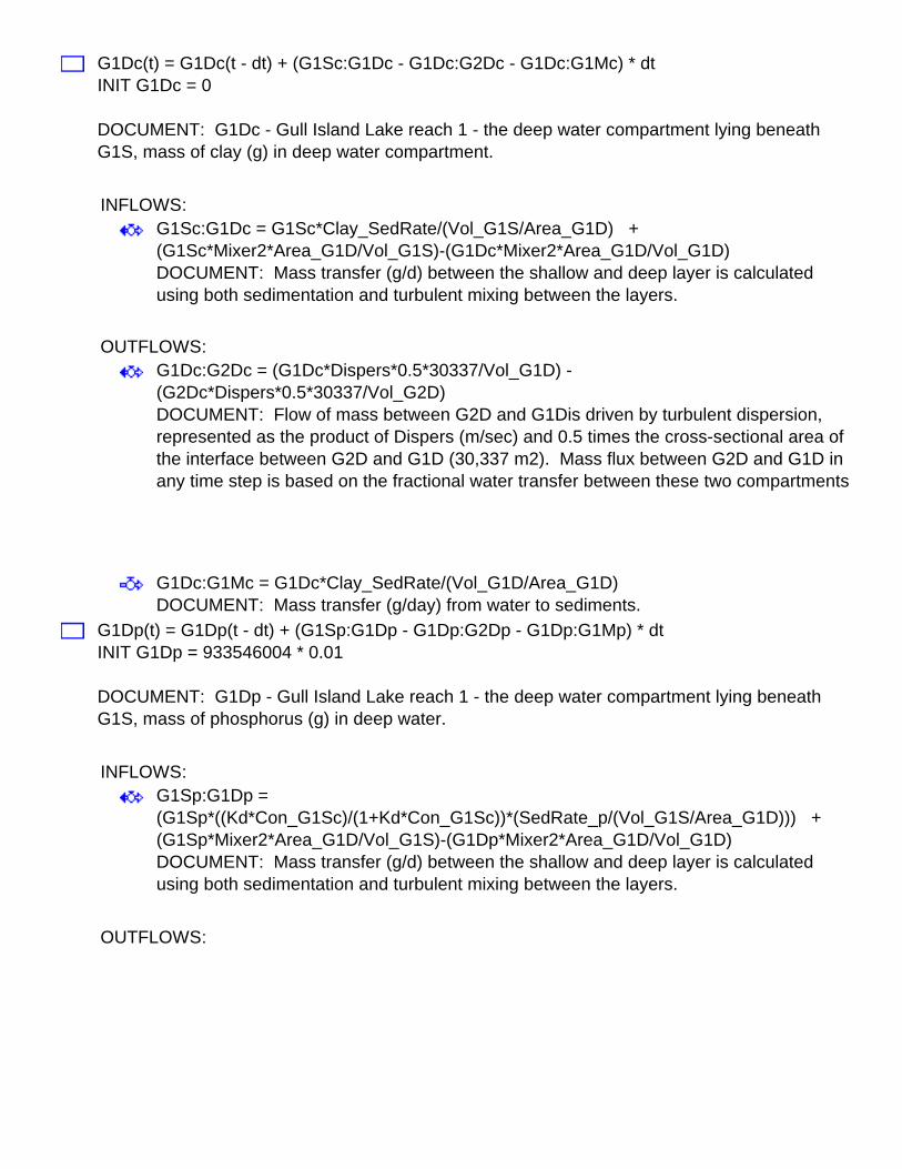
G1Dc(t) = G1Dc(t - dt) + (G1Sc:G1Dc - G1Dc:G2Dc - G1Dc:G1Mc) * dtINIT G1Dc = 0
DOCUMENT: G1Dc - Gull Island Lake reach 1 - the deep water compartment lying beneath G1S, mass of clay (g) in deep water compartment.
INFLOWS:G1Sc:G1Dc = G1Sc*Clay_SedRate/(Vol_G1S/Area_G1D) + (G1Sc*Mixer2*Area_G1D/Vol_G1S)-(G1Dc*Mixer2*Area_G1D/Vol_G1D)DOCUMENT: Mass transfer (g/d) between the shallow and deep layer is calculated using both sedimentation and turbulent mixing between the layers.
OUTFLOWS:G1Dc:G2Dc = (G1Dc*Dispers*0.5*30337/Vol_G1D) - (G2Dc*Dispers*0.5*30337/Vol_G2D)DOCUMENT: Flow of mass between G2D and G1Dis driven by turbulent dispersion, represented as the product of Dispers (m/sec) and 0.5 times the cross-sectional area of the interface between G2D and G1D (30,337 m2). Mass flux between G2D and G1D in any time step is based on the fractional water transfer between these two compartments.
G1Dc:G1Mc = G1Dc*Clay_SedRate/(Vol_G1D/Area_G1D)DOCUMENT: Mass transfer (g/day) from water to sediments.
G1Dp(t) = G1Dp(t - dt) + (G1Sp:G1Dp - G1Dp:G2Dp - G1Dp:G1Mp) * dtINIT G1Dp = 933546004 * 0.01
DOCUMENT: G1Dp - Gull Island Lake reach 1 - the deep water compartment lying beneath G1S, mass of phosphorus (g) in deep water.
INFLOWS:G1Sp:G1Dp = (G1Sp*((Kd*Con_G1Sc)/(1+Kd*Con_G1Sc))*(SedRate_p/(Vol_G1S/Area_G1D))) + (G1Sp*Mixer2*Area_G1D/Vol_G1S)-(G1Dp*Mixer2*Area_G1D/Vol_G1D)DOCUMENT: Mass transfer (g/d) between the shallow and deep layer is calculated using both sedimentation and turbulent mixing between the layers.
OUTFLOWS:
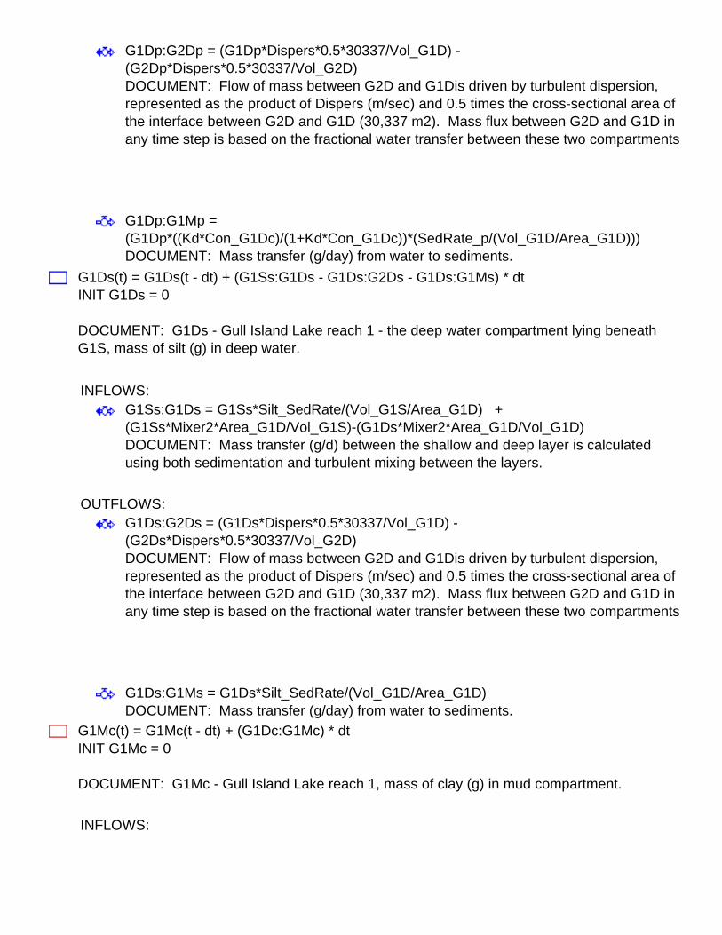
G1Dp:G2Dp = (G1Dp*Dispers*0.5*30337/Vol_G1D) - (G2Dp*Dispers*0.5*30337/Vol_G2D)DOCUMENT: Flow of mass between G2D and G1Dis driven by turbulent dispersion, represented as the product of Dispers (m/sec) and 0.5 times the cross-sectional area of the interface between G2D and G1D (30,337 m2). Mass flux between G2D and G1D in any time step is based on the fractional water transfer between these two compartments.
G1Dp:G1Mp = (G1Dp*((Kd*Con_G1Dc)/(1+Kd*Con_G1Dc))*(SedRate_p/(Vol_G1D/Area_G1D)))DOCUMENT: Mass transfer (g/day) from water to sediments.
G1Ds(t) = G1Ds(t - dt) + (G1Ss:G1Ds - G1Ds:G2Ds - G1Ds:G1Ms) * dtINIT G1Ds = 0
DOCUMENT: G1Ds - Gull Island Lake reach 1 - the deep water compartment lying beneath G1S, mass of silt (g) in deep water.
INFLOWS:G1Ss:G1Ds = G1Ss*Silt_SedRate/(Vol_G1S/Area_G1D) + (G1Ss*Mixer2*Area_G1D/Vol_G1S)-(G1Ds*Mixer2*Area_G1D/Vol_G1D)DOCUMENT: Mass transfer (g/d) between the shallow and deep layer is calculated using both sedimentation and turbulent mixing between the layers.
OUTFLOWS:G1Ds:G2Ds = (G1Ds*Dispers*0.5*30337/Vol_G1D) - (G2Ds*Dispers*0.5*30337/Vol_G2D)DOCUMENT: Flow of mass between G2D and G1Dis driven by turbulent dispersion, represented as the product of Dispers (m/sec) and 0.5 times the cross-sectional area of the interface between G2D and G1D (30,337 m2). Mass flux between G2D and G1D in any time step is based on the fractional water transfer between these two compartments.
G1Ds:G1Ms = G1Ds*Silt_SedRate/(Vol_G1D/Area_G1D)DOCUMENT: Mass transfer (g/day) from water to sediments.
G1Mc(t) = G1Mc(t - dt) + (G1Dc:G1Mc) * dtINIT G1Mc = 0
DOCUMENT: G1Mc - Gull Island Lake reach 1, mass of clay (g) in mud compartment.
INFLOWS:
G1Dc:G1Mc = G1Dc*Clay_SedRate/(Vol_G1D/Area_G1D)DOCUMENT: Mass transfer (g/day) from water to sediments.
G1Mp(t) = G1Mp(t - dt) + (G1Dp:G1Mp) * dtINIT G1Mp = 0
DOCUMENT: G1Mp - Gull Island Lake reach 1, mass of phosporus (g) in mud compartment.
INFLOWS:G1Dp:G1Mp = (G1Dp*((Kd*Con_G1Dc)/(1+Kd*Con_G1Dc))*(SedRate_p/(Vol_G1D/Area_G1D)))DOCUMENT: Mass transfer (g/day) from water to sediments.
G1Ms(t) = G1Ms(t - dt) + (G1Ds:G1Ms) * dtINIT G1Ms = 0
DOCUMENT: G1Ms - Gull Island Lake reach 1, mass of silt (g) in mud compartment.
INFLOWS:G1Ds:G1Ms = G1Ds*Silt_SedRate/(Vol_G1D/Area_G1D)DOCUMENT: Mass transfer (g/day) from water to sediments.
G1Sc(t) = G1Sc(t - dt) + (WSc:G1Sc + Erosion_G1Sc - G1Sc:G2Sc - G1Sc:G1Dc) * dtINIT G1Sc = 0
DOCUMENT: G1Sc - Gull Lake reach 1, mass of clay (g) in surface water compartment - extends from km 148 to km 209 (the sill at the outlet of Lake Winokapau). This is modelled as a stratified water body.
INFLOWS:WSc:G1Sc = WSc*(((Unregulated_Runoff_c * 11256058672) + Churchill_Falls_Flow_c)/Vol_WS)DOCUMENT: Mass of TSS entering G1S from WS is equal to the mass in WS multiplied by the fractional replacement of water in WS
Total water moving through this reach is the sum of water entering from the regulated Churchill Falls flow plus the cumulative unregulated flow. This is calculated as the cumulative watershed area of unregulated drainage into the WS segment (m2) times the seasonally adjusted unregulated runoff (m/d)

Erosion_G1Sc = (Ice_c * (122*1650000/196) * Erosion_Intensity) + ((Unregulated_Runoff_c * 4128937049.923)*TSS_Conc_Clay)DOCUMENT: Amount of Clay (g/day) entering G1S weighted for ice free times of the year
1650000 is the density of silt in g/m3196 = ice free days122 = Eroded Volume of Clay (m3)4128937049.923 = Unregulated Segment Drainage Area (m2)
OUTFLOWS:G1Sc:G2Sc = G1Sc*(((Unregulated_Runoff_c * 15384995722) + Churchill_Falls_Flow_c)/Vol_G1S)DOCUMENT: Mass of TSS entering G2S from G1S is equal to the mass in G1S multiplied by the fractional replacement of water in G1S
Total water moving through this reach is the sum of water entering from the regulated Churchill Falls flow plus the cumulative unregulated flow. This is calculated as the cumulative watershed area of unregulated drainage into the G1S segment (m2) times the seasonally adjusted unregulated runoff (m/d)
G1Sc:G1Dc = G1Sc*Clay_SedRate/(Vol_G1S/Area_G1D) + (G1Sc*Mixer2*Area_G1D/Vol_G1S)-(G1Dc*Mixer2*Area_G1D/Vol_G1D)DOCUMENT: Mass transfer (g/d) between the shallow and deep layer is calculated using both sedimentation and turbulent mixing between the layers.
G1Sp(t) = G1Sp(t - dt) + (WSp:G1Sp + Erosion_G1Sp - G1Sp:G2Sp - G1Sp:G1Dp) * dtINIT G1Sp = 805e6 * 0.01
DOCUMENT: G1Sp - Gull Lake reach 1, mass of phosphorus (g) in surface water compartment - extends from km 148 to km 209 (the sill at the outlet of Lake Winokapau). This is modelled as a stratified water body.
INFLOWS:WSp:G1Sp = WSp*(((Unregulated_Runoff_p * 11256058672) + Churchill_Falls_Flow_p)/Vol_WS)DOCUMENT: Mass of Phosphorous entering G1S from WS is equal to the mass in WS multiplied by the fractional replacement of water in WS
Total water moving through this reach is the sum of water entering from the regulated Churchill Falls flow plus the cumulative unregulated flow. This is calculated as the cumulative watershed area of unregulated drainage into the WS segment (m2) times the seasonally adjusted unregulated runoff (m/d)

Erosion_G1Sp = (Ice_p * (23216*1000/196) * Erosion_Intensity_p) + ((Unregulated_Runoff_p * 4128937049.923)*Baseline_P)+ (Daily_P_Loss * 29324436)DOCUMENT: Amount of Phosphorous (g/day) entering CF from shoreline erosion and decomposion of organic matter in flooded soils and vegetation, adjusted for frozen or ice free times of the year.
1000 = g/kg conversion factor196 = ice free days23216 = Eroded Volume of Phosphorous (kg)4128937049.923 = Unregulated Segment Drainage Area (m2)29324436 = Flooded Segment Area (m2)
OUTFLOWS:G1Sp:G2Sp = G1Sp*(((Unregulated_Runoff_p * 15384995722) + Churchill_Falls_Flow_p)/Vol_G1S)DOCUMENT: Mass of Phosphorous entering G2S from G1S is equal to the mass in G1S multiplied by the fractional replacement of water in G1S
Total water moving through this reach is the sum of water entering from the regulated Churchill Falls flow plus the cumulative unregulated flow. This is calculated as the cumulative watershed area of unregulated drainage into the G1S segment (m2) times the seasonally adjusted unregulated runoff (m/d)
G1Sp:G1Dp = (G1Sp*((Kd*Con_G1Sc)/(1+Kd*Con_G1Sc))*(SedRate_p/(Vol_G1S/Area_G1D))) + (G1Sp*Mixer2*Area_G1D/Vol_G1S)-(G1Dp*Mixer2*Area_G1D/Vol_G1D)DOCUMENT: Mass transfer (g/d) between the shallow and deep layer is calculated using both sedimentation and turbulent mixing between the layers.
G1Ss(t) = G1Ss(t - dt) + (WSs:G1Ss + Erosion_G1s - G1S:G2S - G1Ss:G1Ds) * dtINIT G1Ss = 0
DOCUMENT: G1Ss - Gull Lake reach 1, mass of silt (g) in surface water compartment - extends from km 148 to km 209 (the sill at the outlet of Lake Winokapau). This is modelled as a stratified water body.
INFLOWS:
WSs:G1Ss = WSs*(((Unregulated_Runoff_s * 11256058672) + Churchill_Falls_Flow_s)/Vol_WS)DOCUMENT: Mass of TSS entering G1S from WS is equal to the mass in WS multiplied by the fractional replacement of water in WS
Total water moving through this reach is the sum of water entering from the regulated Churchill Falls flow plus the cumulative unregulated flow. This is calculated as the cumulative watershed area of unregulated drainage into the WS segment (m2) times the seasonally adjusted unregulated runoff (m/d)
Erosion_G1s = (Ice_s * (37482*1650000/196) * Erosion_Intensity) + ((Unregulated_Runoff_s * 4128937049.923)*TSS_Conc_Silt)DOCUMENT: Amount of Silt (g/day) entering G1S weighted for ice free times of the year
16500000 is the density of silt in g/m3196 = ice free days37482 = Eroded Volume of Silt (m3)4128937049.923 = Unregulated Segment Drainage Area (m2)
OUTFLOWS:G1S:G2S = G1Ss*(((Unregulated_Runoff_s * 15384995722) + Churchill_Falls_Flow_s)/Vol_G1S)DOCUMENT: Mass of TSS entering G2S from G1S is equal to the mass in G1S multiplied by the fractional replacement of water in G1S
Total water moving through this reach is the sum of water entering from the regulated Churchill Falls flow plus the cumulative unregulated flow. This is calculated as the cumulative watershed area of unregulated drainage into the G1S segment (m2) times the seasonally adjusted unregulated runoff (m/d)
G1Ss:G1Ds = G1Ss*Silt_SedRate/(Vol_G1S/Area_G1D) + (G1Ss*Mixer2*Area_G1D/Vol_G1S)-(G1Ds*Mixer2*Area_G1D/Vol_G1D)DOCUMENT: Mass transfer (g/d) between the shallow and deep layer is calculated using both sedimentation and turbulent mixing between the layers.
G2Dc(t) = G2Dc(t - dt) + (G1Dc:G2Dc + G2Sc:G2Dc - G2Dc:G2Mc) * dtINIT G2Dc = 0
DOCUMENT: G2Dc - Gull Island Lake reach 2, mass of clay (g) in deep water compartment - the deep water compartment lying beneath G2S.
INFLOWS:

G1Dc:G2Dc = (G1Dc*Dispers*0.5*30337/Vol_G1D) - (G2Dc*Dispers*0.5*30337/Vol_G2D)DOCUMENT: Flow of mass between G2D and G1Dis driven by turbulent dispersion, represented as the product of Dispers (m/sec) and 0.5 times the cross-sectional area of the interface between G2D and G1D (30,337 m2). Mass flux between G2D and G1D in any time step is based on the fractional water transfer between these two compartments.
G2Sc:G2Dc = G2Sc*Clay_SedRate/(Vol_G2S/Area_G2D) + (G2Sc*Mixer2*Area_G2D/Vol_G2S)-(G2Dc*Mixer2*Area_G2D/Vol_G2D)DOCUMENT: Mass transfer (g/d) between the shallow and deep layer is calculated using both sedimentation and turbulent mixing between the layers.
OUTFLOWS:G2Dc:G2Mc = G2Dc*Clay_SedRate/(Vol_G2D/Area_G2D)DOCUMENT: Mass transfer (g/day) from water to sediments.
G2Dp(t) = G2Dp(t - dt) + (G1Dp:G2Dp + G2Sp:G2Dp - G2Dp:G2Mp) * dtINIT G2Dp = 1232917646 * 0.01
DOCUMENT: G2Dp - Gull Island Lake reach 2, mass of phosphorus (g) in deep water compartment - the deep water compartment lying beneath G2S.
INFLOWS:G1Dp:G2Dp = (G1Dp*Dispers*0.5*30337/Vol_G1D) - (G2Dp*Dispers*0.5*30337/Vol_G2D)DOCUMENT: Flow of mass between G2D and G1Dis driven by turbulent dispersion, represented as the product of Dispers (m/sec) and 0.5 times the cross-sectional area of the interface between G2D and G1D (30,337 m2). Mass flux between G2D and G1D in any time step is based on the fractional water transfer between these two compartments.
G2Sp:G2Dp = (G2Sp*((Kd*Con_G2Sc)/(1+Kd*Con_G2Sc))*(SedRate_p/(Vol_G2S/Area_G2D)))+ (G2Sp*Mixer2*Area_G2D/Vol_G2S)-(G2Dp*Mixer2*Area_G2D/Vol_G2D)DOCUMENT: Mass transfer (g/d) between the shallow and deep layer is calculated using both sedimentation and turbulent mixing between the layers.
OUTFLOWS:G2Dp:G2Mp = (G2Dp*((Kd*Con_G2Dc)/(1+Kd*Con_G2Dc))*(SedRate_p/(Vol_G2D/Area_G2D)))DOCUMENT: Mass transfer (g/day) from water to sediments.
G2Ds(t) = G2Ds(t - dt) + (G1Ds:G2Ds + G2Ss:G2Ds - G2Ds:G2Ms) * dtINIT G2Ds = 0
DOCUMENT: G2Ds - Gull Island Lake reach 2, mass of silt (g) in deep water compartment - the deep water compartment lying beneath G2S.
INFLOWS:G1Ds:G2Ds = (G1Ds*Dispers*0.5*30337/Vol_G1D) - (G2Ds*Dispers*0.5*30337/Vol_G2D)DOCUMENT: Flow of mass between G2D and G1Dis driven by turbulent dispersion, represented as the product of Dispers (m/sec) and 0.5 times the cross-sectional area of the interface between G2D and G1D (30,337 m2). Mass flux between G2D and G1D in any time step is based on the fractional water transfer between these two compartments.
G2Ss:G2Ds = G2Ss*Silt_SedRate/(Vol_G2S/Area_G2D) + (G2Ss*Mixer2*Area_G2D/Vol_G2S)-(G2Ds*Mixer2*Area_G2D/Vol_G2D)DOCUMENT: Mass transfer (g/d) between the shallow and deep layer is calculated using both sedimentation and turbulent mixing between the layers.
OUTFLOWS:G2Ds:G2Ms = G2Ds*Silt_SedRate/(Vol_G2D/Area_G2D)DOCUMENT: Mass transfer (g/day) from water to sediments.
G2Mc(t) = G2Mc(t - dt) + (G2Dc:G2Mc) * dtINIT G2Mc = 0
DOCUMENT: G2Mc - Gull Island Lake reach 2, mass of clay (g) in mud compartment.
INFLOWS:G2Dc:G2Mc = G2Dc*Clay_SedRate/(Vol_G2D/Area_G2D)DOCUMENT: Mass transfer (g/day) from water to sediments.
G2Mp(t) = G2Mp(t - dt) + (G2Dp:G2Mp) * dtINIT G2Mp = 0
DOCUMENT: G2Mp - Gull Island Lake reach 2, mass of phosphurus (g) in mud compartment.
INFLOWS:G2Dp:G2Mp = (G2Dp*((Kd*Con_G2Dc)/(1+Kd*Con_G2Dc))*(SedRate_p/(Vol_G2D/Area_G2D)))DOCUMENT: Mass transfer (g/day) from water to sediments.
G2Ms(t) = G2Ms(t - dt) + (G2Ds:G2Ms) * dtINIT G2Ms = 0
DOCUMENT: G2Ms - Gull Island Lake reach 2, mass of silt (g) in mud compartment.
INFLOWS:G2Ds:G2Ms = G2Ds*Silt_SedRate/(Vol_G2D/Area_G2D)DOCUMENT: Mass transfer (g/day) from water to sediments.
G2Sc(t) = G2Sc(t - dt) + (G1Sc:G2Sc + Erosion_G2Sc - G2Sc:ML1c - G2Sc:G2Dc) * dtINIT G2Sc = 0
DOCUMENT: G2Sc - Gull Lake reach 2, mass of clay (g) in surface water compartment - extends from km 102 (the Gull Island dam) to km 148. This is modelled as a stratified water body.
INFLOWS:G1Sc:G2Sc = G1Sc*(((Unregulated_Runoff_c * 15384995722) + Churchill_Falls_Flow_c)/Vol_G1S)DOCUMENT: Mass of TSS entering G2S from G1S is equal to the mass in G1S multiplied by the fractional replacement of water in G1S
Total water moving through this reach is the sum of water entering from the regulated Churchill Falls flow plus the cumulative unregulated flow. This is calculated as the cumulative watershed area of unregulated drainage into the G1S segment (m2) times the seasonally adjusted unregulated runoff (m/d)
Erosion_G2Sc = (Ice_c * (69*1650000/196) * Erosion_Intensity) + ((Unregulated_Runoff_c * 4722646398.915)*TSS_Conc_Clay)DOCUMENT: Amount of Clay (g/day) entering G2S weighted for ice free times of the year
1650000 is the density of silt in g/m3196 = ice free days69 = Eroded Volume of Clay (m3)4722646398.915 = Unregulated Segment Drainage Area (m2)
OUTFLOWS:
G2Sc:ML1c = G2Sc*(((Unregulated_Runoff_c * 20107642121) + Churchill_Falls_Flow_c)/Vol_G2S)DOCUMENT: Mass of TSS entering ML1 from G2S is equal to the mass in G2S multiplied by the fractional replacement of water in G2S
Total water moving through this reach is the sum of water entering from the regulated Churchill Falls flow plus the cumulative unregulated flow. This is calculated as the cumulative watershed area of unregulated drainage into the G2S segment (m2) times the seasonally adjusted unregulated runoff (m/d)
G2Sc:G2Dc = G2Sc*Clay_SedRate/(Vol_G2S/Area_G2D) + (G2Sc*Mixer2*Area_G2D/Vol_G2S)-(G2Dc*Mixer2*Area_G2D/Vol_G2D)DOCUMENT: Mass transfer (g/d) between the shallow and deep layer is calculated using both sedimentation and turbulent mixing between the layers.
G2Sp(t) = G2Sp(t - dt) + (G1Sp:G2Sp + Erosion_G2Sp - G2Sp:ML1p - G2Sp:G2Dp) * dtINIT G2Sp = 985696307.853 * 0.01
DOCUMENT: G2Sp - Gull Lake reach 2, mass of phosphorus (g) in surface water compartment - extends from km 102 (the Gull Island dam) to km 148. This is modelled as a stratified water body.
INFLOWS:G1Sp:G2Sp = G1Sp*(((Unregulated_Runoff_p * 15384995722) + Churchill_Falls_Flow_p)/Vol_G1S)DOCUMENT: Mass of Phosphorous entering G2S from G1S is equal to the mass in G1S multiplied by the fractional replacement of water in G1S
Total water moving through this reach is the sum of water entering from the regulated Churchill Falls flow plus the cumulative unregulated flow. This is calculated as the cumulative watershed area of unregulated drainage into the G1S segment (m2) times the seasonally adjusted unregulated runoff (m/d)
Erosion_G2Sp = (Ice_p * (20244*1000/196) * Erosion_Intensity_p) + ((Unregulated_Runoff_p * 4722646398.915)*Baseline_P)+ (Daily_P_Loss * 35797254)DOCUMENT: Amount of Phosphorous (g/day) entering CF from shoreline erosion and decomposion of organic matter in flooded soils and vegetation, adjusted for frozen or ice free times of the year.
1000 = g/kg conversion factor196 = ice free days20244 = Eroded Volume of Phosphorous (kg)4722646398.915 = Unregulated Segment Drainage Area (m2)35797254 = Flooded Segment Area (m2)
OUTFLOWS:G2Sp:ML1p = G2Sp*(((Unregulated_Runoff_p * 20107642121) + Churchill_Falls_Flow_p)/Vol_G2S)DOCUMENT: Mass of Phosphorous entering ML1 from G2S is equal to the mass in G2S multiplied by the fractional replacement of water in G2S
Total water moving through this reach is the sum of water entering from the regulated Churchill Falls flow plus the cumulative unregulated flow. This is calculated as the cumulative watershed area of unregulated drainage into the G2S segment (m2) times the seasonally adjusted unregulated runoff (m/d)
G2Sp:G2Dp = (G2Sp*((Kd*Con_G2Sc)/(1+Kd*Con_G2Sc))*(SedRate_p/(Vol_G2S/Area_G2D)))+ (G2Sp*Mixer2*Area_G2D/Vol_G2S)-(G2Dp*Mixer2*Area_G2D/Vol_G2D)DOCUMENT: Mass transfer (g/d) between the shallow and deep layer is calculated using both sedimentation and turbulent mixing between the layers.
G2Ss(t) = G2Ss(t - dt) + (G1S:G2S + Erosion_G2s - G2Ss:ML1s - G2Ss:G2Ds) * dtINIT G2Ss = 0
DOCUMENT: G2Ss - Gull Lake reach 2, mass of silt (g) in surface water compartment - extends from km 102 (the Gull Island dam) to km 148. This is modelled as a stratified water body.
INFLOWS:
G1S:G2S = G1Ss*(((Unregulated_Runoff_s * 15384995722) + Churchill_Falls_Flow_s)/Vol_G1S)DOCUMENT: Mass of TSS entering G2S from G1S is equal to the mass in G1S multiplied by the fractional replacement of water in G1S
Total water moving through this reach is the sum of water entering from the regulated Churchill Falls flow plus the cumulative unregulated flow. This is calculated as the cumulative watershed area of unregulated drainage into the G1S segment (m2) times the seasonally adjusted unregulated runoff (m/d)
Erosion_G2s = (Ice_s * (32721*1650000/196) * Erosion_Intensity) + ((Unregulated_Runoff_s * 4722646398.915)*TSS_Conc_Silt)DOCUMENT: Amount of Silt (g/day) entering G2S weighted for ice free times of the year
1650000 is the density of silt in g/m3196 = ice free days32721 = Eroded Volume of Silt (m3)4722646398.915 = Unregulated Segment Drainage Area (m2)
OUTFLOWS:G2Ss:ML1s = G2Ss*(((Unregulated_Runoff_s * 20107642121) + Churchill_Falls_Flow_s)/Vol_G2S)DOCUMENT: Mass of TSS entering ML1 from G2S is equal to the mass in G2S multiplied by the fractional replacement of water in G2S
Total water moving through this reach is the sum of water entering from the regulated Churchill Falls flow plus the cumulative unregulated flow. This is calculated as the cumulative watershed area of unregulated drainage into the G2S segment (m2) times the seasonally adjusted unregulated runoff (m/d)
G2Ss:G2Ds = G2Ss*Silt_SedRate/(Vol_G2S/Area_G2D) + (G2Ss*Mixer2*Area_G2D/Vol_G2S)-(G2Ds*Mixer2*Area_G2D/Vol_G2D)DOCUMENT: Mass transfer (g/d) between the shallow and deep layer is calculated using both sedimentation and turbulent mixing between the layers.
HVc(t) = HVc(t - dt) + (ML3c:HVc + Erosion_HVc - HVc:HVMc - HVc:LMc) * dtINIT HVc = 0
DOCUMENT: HVc - Happy Valley, mass of clay (g) in water compartment - reach of the Churchill river between km 0 and km 43. This reach is downstream of the Muskrat Falls dam and discharges into Lake Melville.
INFLOWS:
ML3c:HVc = ML3c*(((Unregulated_Runoff_c * 22741960833) + Churchill_Falls_Flow_c)/Vol_ML3)DOCUMENT: Mass of TSS entering HVS from ML3 is equal to the mass in ML3 multiplied by the fractional replacement of water in ML3
Total water moving through this reach is the sum of water entering from the regulated Churchill Falls flow plus the cumulative unregulated flow. This is calculated as the cumulative watershed area of unregulated drainage into the ML3 segment (m2) times the seasonally adjusted unregulated runoff (m/d)
Erosion_HVc = (Ice_c * (65765*1650000/196) * Erosion_Intensity) + ((Unregulated_Runoff_c * 1815982274.017)*TSS_Conc_Clay)DOCUMENT: Amount of Clay (g/day) entering HV weighted for ice free times of the year
1650000 is the density of silt in g/m3196 = ice free days65765 = Eroded Volume of Clay (m3)1815982274.017 = Unregulated Segment Drainage Area (m2)
OUTFLOWS:HVc:HVMc = HVc*Clay_SedRate/(Vol_HV/Area_HV)DOCUMENT: Mass transfer (g/day) from water to sediments.HVc:LMc = HVc*(((Unregulated_Runoff_c * 24557943107) + Churchill_Falls_Flow_c)/Vol_HV)DOCUMENT: Mass of TSS entering LM from HVS is equal to the mass in HVS multiplied by the fractional replacement of water in HVS
Total water moving through this reach is the sum of water entering from the regulated Churchill Falls flow plus the cumulative unregulated flow. This is calculated as the cumulative watershed area of unregulated drainage into the HVS segment (m2) times the seasonally adjusted unregulated runoff (m/d)
HVMc(t) = HVMc(t - dt) + (HVc:HVMc) * dtINIT HVMc = 0
DOCUMENT: HVMc - Happy Valley reach, mass of clay (g) in mud compartment.
INFLOWS:HVc:HVMc = HVc*Clay_SedRate/(Vol_HV/Area_HV)DOCUMENT: Mass transfer (g/day) from water to sediments.
HVMp(t) = HVMp(t - dt) + (HVp:HVMp) * dtINIT HVMp = 0
DOCUMENT: HVMp - Happy Valley reach, mass of phosphorus (g) in mud compartment.
INFLOWS:HVp:HVMp = (HVp*((Kd*Con_HVc)/(1+Kd*Con_HVc))*(SedRate_p/(Vol_HV/Area_HV)))DOCUMENT: Mass transfer (g/day) from water to sediments.
HVMs(t) = HVMs(t - dt) + (HVs:HVMs) * dtINIT HVMs = 0
DOCUMENT: HVMs - Happy Valley reach, mass of silt (g) in mud compartment.
INFLOWS:HVs:HVMs = HVs*Silt_SedRate/(Vol_HV/Area_HV)DOCUMENT: Mass transfer (g/day) from water to sediments.
HVp(t) = HVp(t - dt) + (ML3p:HVp + Erosion_HVp - HVp:HVMp - HVp:LMp) * dtINIT HVp = 135046668.453*2 * 0.01
DOCUMENT: HVp - Happy Valley reach, mass of phosphorus (g) in water compartment of the Churchill river between km 0 and km 43. This reach is downstream of the Muskrat Falls dam and discharges into Lake Melville.
INFLOWS:ML3p:HVp = ML3p*(((Unregulated_Runoff_p * 22741960833) + Churchill_Falls_Flow_p)/Vol_ML3)DOCUMENT: Mass of Phosphorous entering HVS from ML3 is equal to the mass in ML3 multiplied by the fractional replacement of water in ML3
Total water moving through this reach is the sum of water entering from the regulated Churchill Falls flow plus the cumulative unregulated flow. This is calculated as the cumulative watershed area of unregulated drainage into the ML3 segment (m2) times the seasonally adjusted unregulated runoff (m/d)
Erosion_HVp = (Ice_p * (304985*1000/196) * Erosion_Intensity_p) + ((Unregulated_Runoff_p * 1815982274.017)*Baseline_P)+ (Daily_P_Loss * 16027654)DOCUMENT: Amount of Phosphorous (g/day) entering CF from shoreline erosion and decomposion of organic matter in flooded soils and vegetation, adjusted for frozen or ice free times of the year.
1000 = g/kg conversion factor196 = ice free days304985 = Eroded Volume of Phosphorous (kg)1815982274.017 = Unregulated Segment Drainage Area (m2)16027654 = Flooded Segment Area (m2)
OUTFLOWS:

HVp:HVMp = (HVp*((Kd*Con_HVc)/(1+Kd*Con_HVc))*(SedRate_p/(Vol_HV/Area_HV)))DOCUMENT: Mass transfer (g/day) from water to sediments.HVp:LMp = HVp*(((Unregulated_Runoff_p * 24557943107) + Churchill_Falls_Flow_p)/Vol_HV)DOCUMENT: Mass of Phosphorous entering LM from HVS is equal to the mass in HVS multiplied by the fractional replacement of water in HVS
Total water moving through this reach is the sum of water entering from the regulated Churchill Falls flow plus the cumulative unregulated flow. This is calculated as the cumulative watershed area of unregulated drainage into the HVS segment (m2) times the seasonally adjusted unregulated runoff (m/d)
HVs(t) = HVs(t - dt) + (ML3s:HVs + Erosion_HVs - HVs:HVMs - HVs:LMs) * dtINIT HVs = 0
DOCUMENT: HVs - Happy Valley reach of the Churchill river, mass of silt (g) in the water compartment between km 0 and km 43. This reach is downstream of the Muskrat Falls dam and discharges into Lake Melville.
INFLOWS:ML3s:HVs = ML3s*(((Unregulated_Runoff_s * 22741960833) + Churchill_Falls_Flow_s)/Vol_ML3)DOCUMENT: Mass of TSS entering HVS from ML3 is equal to the mass in ML3 multiplied by the fractional replacement of water in ML3
Total water moving through this reach is the sum of water entering from the regulated Churchill Falls flow plus the cumulative unregulated flow. This is calculated as the cumulative watershed area of unregulated drainage into the ML3 segment (m2) times the seasonally adjusted unregulated runoff (m/d)
Erosion_HVs = (Ice_s * (428239*1650000/196) * Erosion_Intensity) + ((Unregulated_Runoff_s * 1815982274.017)*TSS_Conc_Silt)DOCUMENT: Amount of Silt (g/day) entering HV weighted for ice free times of the year
1650000 is the density of silt in g/m3196 = ice free days428239 = Eroded Volume of Silt (m3)1815982274.017 = Unregulated Segment Drainage Area (m2)
OUTFLOWS:HVs:HVMs = HVs*Silt_SedRate/(Vol_HV/Area_HV)DOCUMENT: Mass transfer (g/day) from water to sediments.

HVs:LMs = HVs*(((Unregulated_Runoff_s * 24557943107) + Churchill_Falls_Flow_s)/Vol_HV)DOCUMENT: Mass of TSS entering LM from HVS is equal to the mass in HVS multiplied by the fractional replacement of water in HVS
Total water moving through this reach is the sum of water entering from the regulated Churchill Falls flow plus the cumulative unregulated flow. This is calculated as the cumulative watershed area of unregulated drainage into the HVS segment (m2) times the seasonally adjusted unregulated runoff (m/d)
LMc(t) = LMc(t - dt) + (HVc:LMc) * dtINIT LMc = 0
DOCUMENT: LMc - Lake Melville, mass of clay (g). Lake Melville is the ultimate destination and sink for TSS. Concentrations of TSS in lake Melville water are not calculated.
INFLOWS:HVc:LMc = HVc*(((Unregulated_Runoff_c * 24557943107) + Churchill_Falls_Flow_c)/Vol_HV)DOCUMENT: Mass of TSS entering LM from HVS is equal to the mass in HVS multiplied by the fractional replacement of water in HVS
Total water moving through this reach is the sum of water entering from the regulated Churchill Falls flow plus the cumulative unregulated flow. This is calculated as the cumulative watershed area of unregulated drainage into the HVS segment (m2) times the seasonally adjusted unregulated runoff (m/d)
LMp(t) = LMp(t - dt) + (HVp:LMp) * dtINIT LMp = 0
DOCUMENT: LMp - Lake Melville, mass of phosphorus (g). Lake Melville is the ultimate destination and sink for phosphorus. Concentrations of phosphorus in lake Melville water are not calculated.
INFLOWS:HVp:LMp = HVp*(((Unregulated_Runoff_p * 24557943107) + Churchill_Falls_Flow_p)/Vol_HV)DOCUMENT: Mass of Phosphorous entering LM from HVS is equal to the mass in HVS multiplied by the fractional replacement of water in HVS
Total water moving through this reach is the sum of water entering from the regulated Churchill Falls flow plus the cumulative unregulated flow. This is calculated as the cumulative watershed area of unregulated drainage into the HVS segment (m2) times the seasonally adjusted unregulated runoff (m/d)
LMs(t) = LMs(t - dt) + (HVs:LMs) * dtINIT LMs = 0
DOCUMENT: LMs - Lake Melville, mass of silt (g). Lake Melville is the ultimate destination and sink for TSS. Concentrations of TSS in lake Melville water are not calculated.
INFLOWS:HVs:LMs = HVs*(((Unregulated_Runoff_s * 24557943107) + Churchill_Falls_Flow_s)/Vol_HV)DOCUMENT: Mass of TSS entering LM from HVS is equal to the mass in HVS multiplied by the fractional replacement of water in HVS
Total water moving through this reach is the sum of water entering from the regulated Churchill Falls flow plus the cumulative unregulated flow. This is calculated as the cumulative watershed area of unregulated drainage into the HVS segment (m2) times the seasonally adjusted unregulated runoff (m/d)
ML1c(t) = ML1c(t - dt) + (G2Sc:ML1c + Erosion_ML1c - ML1c:ML2c - ML1c:ML1Mc) * dtINIT ML1c = 0
DOCUMENT: ML1c - Muskrat Lake Reach 1, mass of clay (g) in water compartment. This extends from km 88 to km 102 (the toe of the Gull Island dam), and is modelled as a fully mixed water body.
INFLOWS:G2Sc:ML1c = G2Sc*(((Unregulated_Runoff_c * 20107642121) + Churchill_Falls_Flow_c)/Vol_G2S)DOCUMENT: Mass of TSS entering ML1 from G2S is equal to the mass in G2S multiplied by the fractional replacement of water in G2S
Total water moving through this reach is the sum of water entering from the regulated Churchill Falls flow plus the cumulative unregulated flow. This is calculated as the cumulative watershed area of unregulated drainage into the G2S segment (m2) times the seasonally adjusted unregulated runoff (m/d)
Erosion_ML1c = (Ice_c * (92632*1650000/196) * Erosion_Intensity) + ((Unregulated_Runoff_c * 569404091.164)*TSS_Conc_Clay)DOCUMENT: Amount of Clay (g/day) entering ML1 weighted for ice free times of the year
1650000 is the density of silt in g/m3196 = ice free days92632 = Eroded Volume of Clay (m3)569404091.164 = Unregulated Segment Drainage Area (m2)
OUTFLOWS:
ML1c:ML2c = ML1c*(((Unregulated_Runoff_c * 20677046212) + Churchill_Falls_Flow_c)/Vol_ML1)DOCUMENT: Mass of TSS entering ML2 from ML1 is equal to the mass in ML1 multiplied by the fractional replacement of water in ML1
Total water moving through this reach is the sum of water entering from the regulated Churchill Falls flow plus the cumulative unregulated flow. This is calculated as the cumulative watershed area of unregulated drainage into the ML1 segment (m2) times the seasonally adjusted unregulated runoff (m/d)
ML1c:ML1Mc = ML1c*Clay_SedRate/(Vol_ML1/Area_ML1)DOCUMENT: Mass transfer (g/day) from water to sediments.
ML1Mc(t) = ML1Mc(t - dt) + (ML1c:ML1Mc) * dtINIT ML1Mc = 0
DOCUMENT: ML1Mc - Muskrat Lake Reach 1, mass of clay (g) in mud compartment.
INFLOWS:ML1c:ML1Mc = ML1c*Clay_SedRate/(Vol_ML1/Area_ML1)DOCUMENT: Mass transfer (g/day) from water to sediments.
ML1Mp(t) = ML1Mp(t - dt) + (ML1p:ML1Mp) * dtINIT ML1Mp = 0
DOCUMENT: ML1Mp - Muskrat Lake Reach 1, mass of phosphorus (g) in mud compartment.
INFLOWS:ML1p:ML1Mp = (ML1p*((Kd*Con_ML1c)/(1+Kd*Con_ML1c))*(SedRate_p/(Vol_ML1/Area_ML1)))DOCUMENT: Mass transfer (g/day) from water to sediments.
ML1Ms(t) = ML1Ms(t - dt) + (ML1s:ML1Ms) * dtINIT ML1Ms = 0
DOCUMENT: ML1Ms - Muskrat Lake Reach 1, mass of silt (g) in mud compartment.
INFLOWS:ML1s:ML1Ms = ML1s*Silt_SedRate/(Vol_ML1/Area_ML1)DOCUMENT: Mass transfer (g/day) from water to sediments.
ML1p(t) = ML1p(t - dt) + (G2Sp:ML1p + Erosion_ML1p - ML1p:ML2p - ML1p:ML1Mp) * dtINIT ML1p = 381092553 * 0.01
DOCUMENT: ML1p - Muskrat Lake Reach 1, mass of phosphorus (g) in water compartment. This extends from km 88 to km 102 (the toe of the Gull Island dam), and is modelled as a fully mixed water body.
INFLOWS:G2Sp:ML1p = G2Sp*(((Unregulated_Runoff_p * 20107642121) + Churchill_Falls_Flow_p)/Vol_G2S)DOCUMENT: Mass of Phosphorous entering ML1 from G2S is equal to the mass in G2S multiplied by the fractional replacement of water in G2S
Total water moving through this reach is the sum of water entering from the regulated Churchill Falls flow plus the cumulative unregulated flow. This is calculated as the cumulative watershed area of unregulated drainage into the G2S segment (m2) times the seasonally adjusted unregulated runoff (m/d)
Erosion_ML1p = (Ice_p * (288222*1000/196) * Erosion_Intensity_p) + ((Unregulated_Runoff_p * 569404091.164)*Baseline_P)+ (Daily_P_Loss * 4514911)DOCUMENT: Amount of Phosphorous (g/day) entering CF from shoreline erosion and decomposion of organic matter in flooded soils and vegetation, adjusted for frozen or ice free times of the year.
1000 = g/kg conversion factor196 = ice free days288222 = Eroded Volume of Phosphorous (kg)569404091.164 = Unregulated Segment Drainage Area (m2)4514911 = Flooded Segment Area (m2)
OUTFLOWS:ML1p:ML2p = ML1p*(((Unregulated_Runoff_p * 20677046212) + Churchill_Falls_Flow_p)/Vol_ML1)DOCUMENT: Mass of Phosphorous entering ML2 from ML1 is equal to the mass in ML1 multiplied by the fractional replacement of water in ML1
Total water moving through this reach is the sum of water entering from the regulated Churchill Falls flow plus the cumulative unregulated flow. This is calculated as the cumulative watershed area of unregulated drainage into the ML1 segment (m2) times the seasonally adjusted unregulated runoff (m/d)
ML1p:ML1Mp = (ML1p*((Kd*Con_ML1c)/(1+Kd*Con_ML1c))*(SedRate_p/(Vol_ML1/Area_ML1)))DOCUMENT: Mass transfer (g/day) from water to sediments.
ML1s(t) = ML1s(t - dt) + (G2Ss:ML1s + Erosion_ML1s - ML1s:ML2s - ML1s:ML1Ms) * dtINIT ML1s = 0
DOCUMENT: ML1s - Muskrat Lake Reach 1, mass of silt (g) in surface water compartment. This extends from km 88 to km 102 (the toe of the Gull Island dam), and is modelled as a fully mixed water body.

INFLOWS:G2Ss:ML1s = G2Ss*(((Unregulated_Runoff_s * 20107642121) + Churchill_Falls_Flow_s)/Vol_G2S)DOCUMENT: Mass of TSS entering ML1 from G2S is equal to the mass in G2S multiplied by the fractional replacement of water in G2S
Total water moving through this reach is the sum of water entering from the regulated Churchill Falls flow plus the cumulative unregulated flow. This is calculated as the cumulative watershed area of unregulated drainage into the G2S segment (m2) times the seasonally adjusted unregulated runoff (m/d)
Erosion_ML1s = (Ice_s * (374220*1650000/196) * Erosion_Intensity) + ((Unregulated_Runoff_s * 569404091.164)*TSS_Conc_Silt)DOCUMENT: Amount of Silt (g/day) entering ML1 weighted for ice free times of the year
1650000 is the density of silt in g/m3196 = ice free days374220 = Eroded Volume of Silt (m3)569404091.164 = Unregulated Segment Drainage Area (m2)
OUTFLOWS:ML1s:ML2s = ML1s*(((Unregulated_Runoff_s * 20677046212) + Churchill_Falls_Flow_s)/Vol_ML1)DOCUMENT: Mass of TSS entering ML2 from ML1 is equal to the mass in ML1 multiplied by the fractional replacement of water in ML1
Total water moving through this reach is the sum of water entering from the regulated Churchill Falls flow plus the cumulative unregulated flow. This is calculated as the cumulative watershed area of unregulated drainage into the ML1 segment (m2) times the seasonally adjusted unregulated runoff (m/d)
ML1s:ML1Ms = ML1s*Silt_SedRate/(Vol_ML1/Area_ML1)DOCUMENT: Mass transfer (g/day) from water to sediments.
ML2c(t) = ML2c(t - dt) + (ML1c:ML2c + Erosion_ML2c - ML2c:ML3c - ML2c:ML2Mc) * dtINIT ML2c = 0
DOCUMENT: ML2c - Muskrat Lake Reach 2, mass of clay (g) in water compartment. This extends from km 69 to km 88, and is modelled as a fully mixed water body.
INFLOWS:
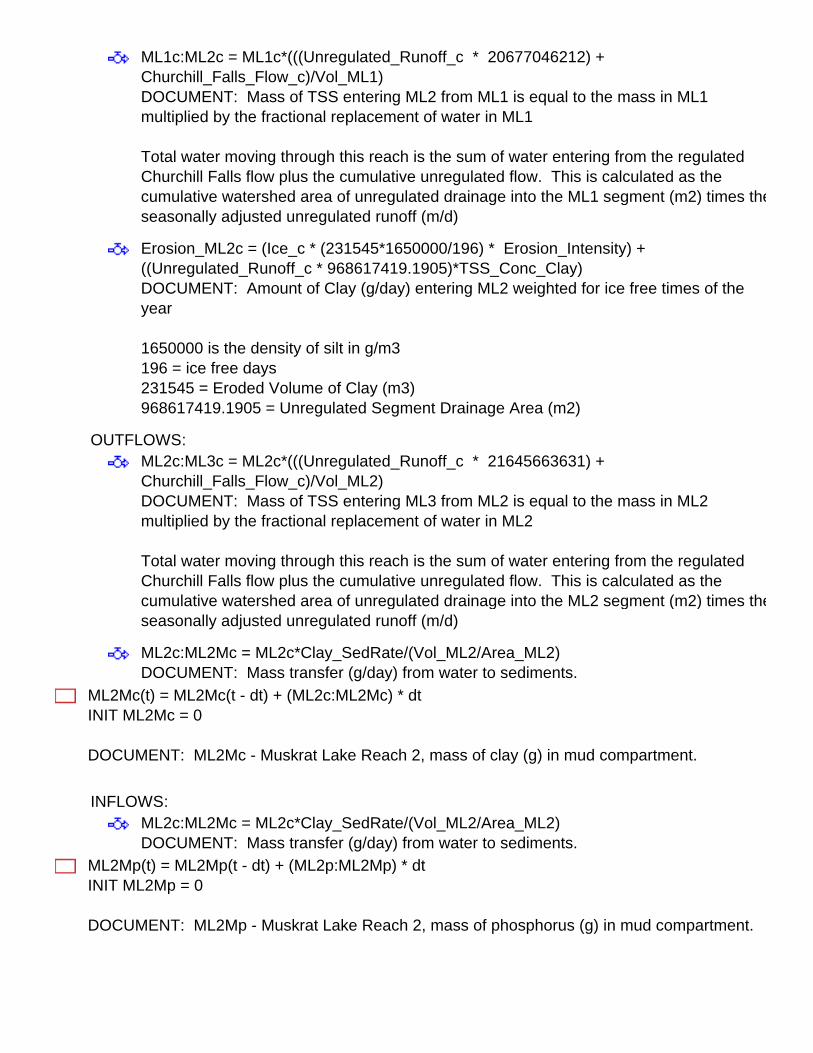
ML1c:ML2c = ML1c*(((Unregulated_Runoff_c * 20677046212) + Churchill_Falls_Flow_c)/Vol_ML1)DOCUMENT: Mass of TSS entering ML2 from ML1 is equal to the mass in ML1 multiplied by the fractional replacement of water in ML1
Total water moving through this reach is the sum of water entering from the regulated Churchill Falls flow plus the cumulative unregulated flow. This is calculated as the cumulative watershed area of unregulated drainage into the ML1 segment (m2) times the seasonally adjusted unregulated runoff (m/d)
Erosion_ML2c = (Ice_c * (231545*1650000/196) * Erosion_Intensity) + ((Unregulated_Runoff_c * 968617419.1905)*TSS_Conc_Clay)DOCUMENT: Amount of Clay (g/day) entering ML2 weighted for ice free times of the year
1650000 is the density of silt in g/m3196 = ice free days231545 = Eroded Volume of Clay (m3)968617419.1905 = Unregulated Segment Drainage Area (m2)
OUTFLOWS:ML2c:ML3c = ML2c*(((Unregulated_Runoff_c * 21645663631) + Churchill_Falls_Flow_c)/Vol_ML2)DOCUMENT: Mass of TSS entering ML3 from ML2 is equal to the mass in ML2 multiplied by the fractional replacement of water in ML2
Total water moving through this reach is the sum of water entering from the regulated Churchill Falls flow plus the cumulative unregulated flow. This is calculated as the cumulative watershed area of unregulated drainage into the ML2 segment (m2) times the seasonally adjusted unregulated runoff (m/d)
ML2c:ML2Mc = ML2c*Clay_SedRate/(Vol_ML2/Area_ML2)DOCUMENT: Mass transfer (g/day) from water to sediments.
ML2Mc(t) = ML2Mc(t - dt) + (ML2c:ML2Mc) * dtINIT ML2Mc = 0
DOCUMENT: ML2Mc - Muskrat Lake Reach 2, mass of clay (g) in mud compartment.
INFLOWS:ML2c:ML2Mc = ML2c*Clay_SedRate/(Vol_ML2/Area_ML2)DOCUMENT: Mass transfer (g/day) from water to sediments.
ML2Mp(t) = ML2Mp(t - dt) + (ML2p:ML2Mp) * dtINIT ML2Mp = 0
DOCUMENT: ML2Mp - Muskrat Lake Reach 2, mass of phosphorus (g) in mud compartment.
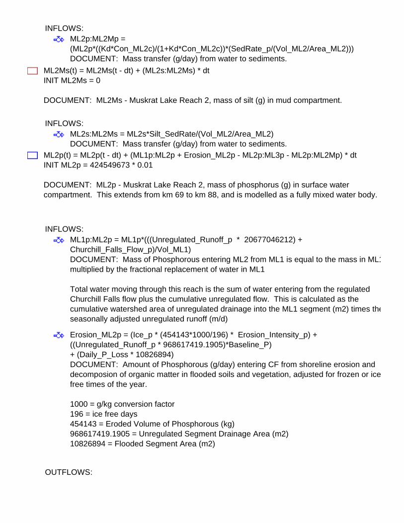
INFLOWS:ML2p:ML2Mp = (ML2p*((Kd*Con_ML2c)/(1+Kd*Con_ML2c))*(SedRate_p/(Vol_ML2/Area_ML2)))DOCUMENT: Mass transfer (g/day) from water to sediments.
ML2Ms(t) = ML2Ms(t - dt) + (ML2s:ML2Ms) * dtINIT ML2Ms = 0
DOCUMENT: ML2Ms - Muskrat Lake Reach 2, mass of silt (g) in mud compartment.
INFLOWS:ML2s:ML2Ms = ML2s*Silt_SedRate/(Vol_ML2/Area_ML2)DOCUMENT: Mass transfer (g/day) from water to sediments.
ML2p(t) = ML2p(t - dt) + (ML1p:ML2p + Erosion_ML2p - ML2p:ML3p - ML2p:ML2Mp) * dtINIT ML2p = 424549673 * 0.01
DOCUMENT: ML2p - Muskrat Lake Reach 2, mass of phosphorus (g) in surface water compartment. This extends from km 69 to km 88, and is modelled as a fully mixed water body.
INFLOWS:ML1p:ML2p = ML1p*(((Unregulated_Runoff_p * 20677046212) + Churchill_Falls_Flow_p)/Vol_ML1)DOCUMENT: Mass of Phosphorous entering ML2 from ML1 is equal to the mass in ML1 multiplied by the fractional replacement of water in ML1
Total water moving through this reach is the sum of water entering from the regulated Churchill Falls flow plus the cumulative unregulated flow. This is calculated as the cumulative watershed area of unregulated drainage into the ML1 segment (m2) times the seasonally adjusted unregulated runoff (m/d)
Erosion_ML2p = (Ice_p * (454143*1000/196) * Erosion_Intensity_p) + ((Unregulated_Runoff_p * 968617419.1905)*Baseline_P)+ (Daily_P_Loss * 10826894)DOCUMENT: Amount of Phosphorous (g/day) entering CF from shoreline erosion and decomposion of organic matter in flooded soils and vegetation, adjusted for frozen or ice free times of the year.
1000 = g/kg conversion factor196 = ice free days454143 = Eroded Volume of Phosphorous (kg)968617419.1905 = Unregulated Segment Drainage Area (m2)10826894 = Flooded Segment Area (m2)
OUTFLOWS:
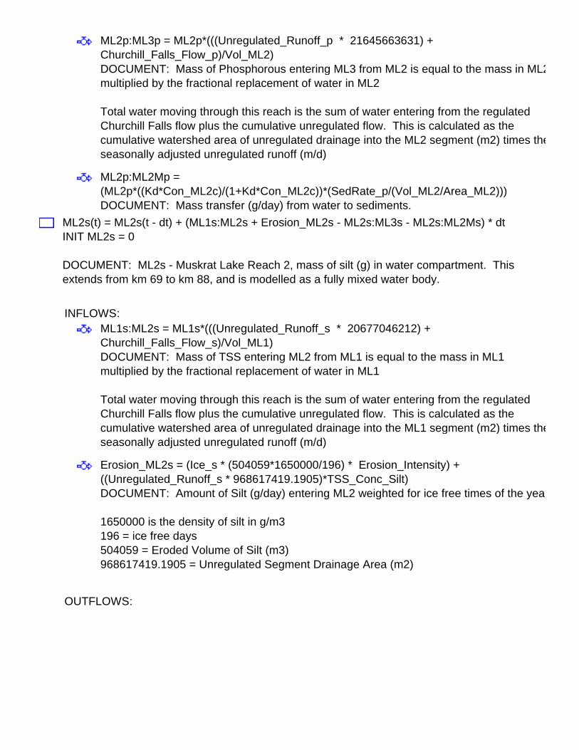
ML2p:ML3p = ML2p*(((Unregulated_Runoff_p * 21645663631) + Churchill_Falls_Flow_p)/Vol_ML2)DOCUMENT: Mass of Phosphorous entering ML3 from ML2 is equal to the mass in ML2 multiplied by the fractional replacement of water in ML2
Total water moving through this reach is the sum of water entering from the regulated Churchill Falls flow plus the cumulative unregulated flow. This is calculated as the cumulative watershed area of unregulated drainage into the ML2 segment (m2) times the seasonally adjusted unregulated runoff (m/d)
ML2p:ML2Mp = (ML2p*((Kd*Con_ML2c)/(1+Kd*Con_ML2c))*(SedRate_p/(Vol_ML2/Area_ML2)))DOCUMENT: Mass transfer (g/day) from water to sediments.
ML2s(t) = ML2s(t - dt) + (ML1s:ML2s + Erosion_ML2s - ML2s:ML3s - ML2s:ML2Ms) * dtINIT ML2s = 0
DOCUMENT: ML2s - Muskrat Lake Reach 2, mass of silt (g) in water compartment. This extends from km 69 to km 88, and is modelled as a fully mixed water body.
INFLOWS:ML1s:ML2s = ML1s*(((Unregulated_Runoff_s * 20677046212) + Churchill_Falls_Flow_s)/Vol_ML1)DOCUMENT: Mass of TSS entering ML2 from ML1 is equal to the mass in ML1 multiplied by the fractional replacement of water in ML1
Total water moving through this reach is the sum of water entering from the regulated Churchill Falls flow plus the cumulative unregulated flow. This is calculated as the cumulative watershed area of unregulated drainage into the ML1 segment (m2) times the seasonally adjusted unregulated runoff (m/d)
Erosion_ML2s = (Ice_s * (504059*1650000/196) * Erosion_Intensity) + ((Unregulated_Runoff_s * 968617419.1905)*TSS_Conc_Silt)DOCUMENT: Amount of Silt (g/day) entering ML2 weighted for ice free times of the year
1650000 is the density of silt in g/m3196 = ice free days504059 = Eroded Volume of Silt (m3)968617419.1905 = Unregulated Segment Drainage Area (m2)
OUTFLOWS:

ML2s:ML3s = ML2s*(((Unregulated_Runoff_s * 21645663631) + Churchill_Falls_Flow_s)/Vol_ML2)DOCUMENT: Mass of TSS entering ML3 from ML2 is equal to the mass in ML2 multiplied by the fractional replacement of water in ML2
Total water moving through this reach is the sum of water entering from the regulated Churchill Falls flow plus the cumulative unregulated flow. This is calculated as the cumulative watershed area of unregulated drainage into the ML2 segment (m2) times the seasonally adjusted unregulated runoff (m/d)
ML2s:ML2Ms = ML2s*Silt_SedRate/(Vol_ML2/Area_ML2)DOCUMENT: Mass transfer (g/day) from water to sediments.
ML3c(t) = ML3c(t - dt) + (ML2c:ML3c + Erosion_ML3c - ML3c:HVc - ML3c:ML3Mc) * dtINIT ML3c = 0
DOCUMENT: ML3c - Muskrat Lake Reach 3, mass of clay (g) in water compartment. This extends from km 43 to km 69, and is modelled as a fully mixed water body.
INFLOWS:ML2c:ML3c = ML2c*(((Unregulated_Runoff_c * 21645663631) + Churchill_Falls_Flow_c)/Vol_ML2)DOCUMENT: Mass of TSS entering ML3 from ML2 is equal to the mass in ML2 multiplied by the fractional replacement of water in ML2
Total water moving through this reach is the sum of water entering from the regulated Churchill Falls flow plus the cumulative unregulated flow. This is calculated as the cumulative watershed area of unregulated drainage into the ML2 segment (m2) times the seasonally adjusted unregulated runoff (m/d)
Erosion_ML3c = (Ice_c * (216190*1650000/196) * Erosion_Intensity) + ((Unregulated_Runoff_c * 1096297202.038)*TSS_Conc_Clay)DOCUMENT: Amount of Clay (g/day) entering ML3 weighted for ice free times of the year
1650000 is the density of silt in g/m3196 = ice free days216190 = Eroded Volume of Clay (m3)1096297202.038 = Unregulated Segment Drainage Area (m2)
OUTFLOWS:

ML3c:HVc = ML3c*(((Unregulated_Runoff_c * 22741960833) + Churchill_Falls_Flow_c)/Vol_ML3)DOCUMENT: Mass of TSS entering HVS from ML3 is equal to the mass in ML3 multiplied by the fractional replacement of water in ML3
Total water moving through this reach is the sum of water entering from the regulated Churchill Falls flow plus the cumulative unregulated flow. This is calculated as the cumulative watershed area of unregulated drainage into the ML3 segment (m2) times the seasonally adjusted unregulated runoff (m/d)
ML3c:ML3Mc = ML3c*Clay_SedRate/(Vol_ML3/Area_ML3)DOCUMENT: Mass transfer (g/day) from water to sediments.
ML3Mc(t) = ML3Mc(t - dt) + (ML3c:ML3Mc) * dtINIT ML3Mc = 0
DOCUMENT: ML3Mc - Muskrat Lake Reach 3, mass of clay (g) in mud compartment.
INFLOWS:ML3c:ML3Mc = ML3c*Clay_SedRate/(Vol_ML3/Area_ML3)DOCUMENT: Mass transfer (g/day) from water to sediments.
ML3Mp(t) = ML3Mp(t - dt) + (ML3p:ML3Mp) * dtINIT ML3Mp = 0
DOCUMENT: ML3Mp - Muskrat Lake Reach 3, mass of phosphorus (g) in mud compartment.
INFLOWS:ML3p:ML3Mp = (ML3p*((Kd*Con_ML3c)/(1+Kd*Con_ML3c))*(SedRate_p/(Vol_ML3/Area_ML3)))DOCUMENT: Mass transfer (g/day) from water to sediments.
ML3Ms(t) = ML3Ms(t - dt) + (ML3s:ML3Ms) * dtINIT ML3Ms = 0
DOCUMENT: ML3Ms - Muskrat Lake Reach 3, mass of silt (g) in mud compartment.
INFLOWS:ML3s:ML3Ms = ML3s*Silt_SedRate/(Vol_ML3/Area_ML3)DOCUMENT: Mass transfer (g/day) from water to sediments.
ML3p(t) = ML3p(t - dt) + (ML2p:ML3p + Erosion_ML3p - ML3p:HVp - ML3p:ML3Mp) * dtINIT ML3p = 900733511 * 0.01
DOCUMENT: ML3p - Muskrat Lake Reach 3, mass of phosphorus (g) in water compartment. This extends from km 43 to km 69, and is modelled as a fully mixed water body.
INFLOWS:
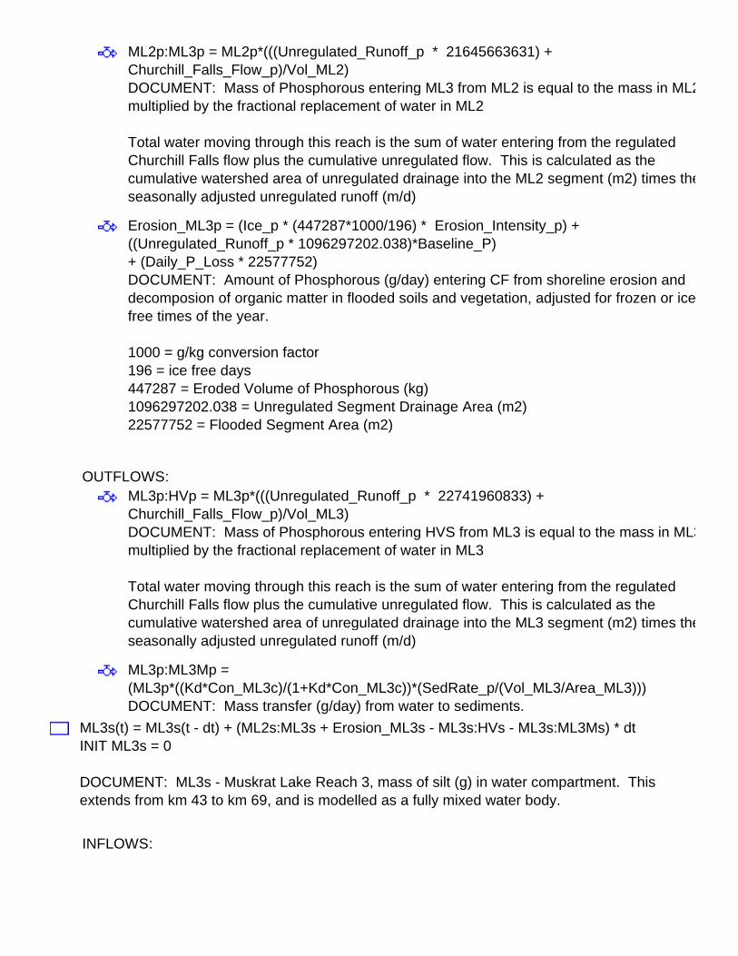
ML2p:ML3p = ML2p*(((Unregulated_Runoff_p * 21645663631) + Churchill_Falls_Flow_p)/Vol_ML2)DOCUMENT: Mass of Phosphorous entering ML3 from ML2 is equal to the mass in ML2 multiplied by the fractional replacement of water in ML2
Total water moving through this reach is the sum of water entering from the regulated Churchill Falls flow plus the cumulative unregulated flow. This is calculated as the cumulative watershed area of unregulated drainage into the ML2 segment (m2) times the seasonally adjusted unregulated runoff (m/d)
Erosion_ML3p = (Ice_p * (447287*1000/196) * Erosion_Intensity_p) + ((Unregulated_Runoff_p * 1096297202.038)*Baseline_P)+ (Daily_P_Loss * 22577752)DOCUMENT: Amount of Phosphorous (g/day) entering CF from shoreline erosion and decomposion of organic matter in flooded soils and vegetation, adjusted for frozen or ice free times of the year.
1000 = g/kg conversion factor196 = ice free days447287 = Eroded Volume of Phosphorous (kg)1096297202.038 = Unregulated Segment Drainage Area (m2)22577752 = Flooded Segment Area (m2)
OUTFLOWS:ML3p:HVp = ML3p*(((Unregulated_Runoff_p * 22741960833) + Churchill_Falls_Flow_p)/Vol_ML3)DOCUMENT: Mass of Phosphorous entering HVS from ML3 is equal to the mass in ML3 multiplied by the fractional replacement of water in ML3
Total water moving through this reach is the sum of water entering from the regulated Churchill Falls flow plus the cumulative unregulated flow. This is calculated as the cumulative watershed area of unregulated drainage into the ML3 segment (m2) times the seasonally adjusted unregulated runoff (m/d)
ML3p:ML3Mp = (ML3p*((Kd*Con_ML3c)/(1+Kd*Con_ML3c))*(SedRate_p/(Vol_ML3/Area_ML3)))DOCUMENT: Mass transfer (g/day) from water to sediments.
ML3s(t) = ML3s(t - dt) + (ML2s:ML3s + Erosion_ML3s - ML3s:HVs - ML3s:ML3Ms) * dtINIT ML3s = 0
DOCUMENT: ML3s - Muskrat Lake Reach 3, mass of silt (g) in water compartment. This extends from km 43 to km 69, and is modelled as a fully mixed water body.
INFLOWS:

ML2s:ML3s = ML2s*(((Unregulated_Runoff_s * 21645663631) + Churchill_Falls_Flow_s)/Vol_ML2)DOCUMENT: Mass of TSS entering ML3 from ML2 is equal to the mass in ML2 multiplied by the fractional replacement of water in ML2
Total water moving through this reach is the sum of water entering from the regulated Churchill Falls flow plus the cumulative unregulated flow. This is calculated as the cumulative watershed area of unregulated drainage into the ML2 segment (m2) times the seasonally adjusted unregulated runoff (m/d)
Erosion_ML3s = (Ice_s * (508310*1650000/196) * Erosion_Intensity) + ((Unregulated_Runoff_s * 1096297202.038)*TSS_Conc_Silt)DOCUMENT: Amount of Silt (g/day) entering ML3 weighted for ice free times of the year
1650000 is the density of silt in g/m3196 = ice free days508310 = Eroded Volume of Silt (m3)1096297202.038 = Unregulated Segment Drainage Area (m2)
OUTFLOWS:ML3s:HVs = ML3s*(((Unregulated_Runoff_s * 22741960833) + Churchill_Falls_Flow_s)/Vol_ML3)DOCUMENT: Mass of TSS entering HVS from ML3 is equal to the mass in ML3 multiplied by the fractional replacement of water in ML3
Total water moving through this reach is the sum of water entering from the regulated Churchill Falls flow plus the cumulative unregulated flow. This is calculated as the cumulative watershed area of unregulated drainage into the ML3 segment (m2) times the seasonally adjusted unregulated runoff (m/d)
ML3s:ML3Ms = ML3s*Silt_SedRate/(Vol_ML3/Area_ML3)DOCUMENT: Mass transfer (g/day) from water to sediments.
WDc(t) = WDc(t - dt) + (WSc:WDc - WDc:WMc) * dtINIT WDc = 0
DOCUMENT: WDc - Winokapau Lake, deep water compartment lying beneath WS, mass of clay (g) in water compartment.
INFLOWS:WSc:WDc = WSc*Clay_SedRate/(Vol_WS/Area_WD) + (WSc*Mixer2*Area_WD/Vol_WS)-(WDc*Mixer2*Area_WD/Vol_WD)DOCUMENT: Mass transfer (g/d) between the shallow and deep layer is calculated using both sedimentation and turbulent mixing between the layers.
OUTFLOWS:
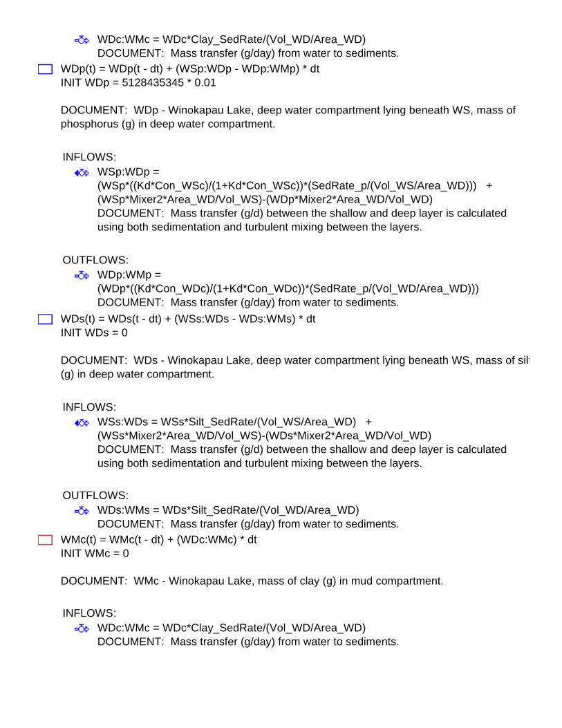
WDc:WMc = WDc*Clay_SedRate/(Vol_WD/Area_WD)DOCUMENT: Mass transfer (g/day) from water to sediments.
WDp(t) = WDp(t - dt) + (WSp:WDp - WDp:WMp) * dtINIT WDp = 5128435345 * 0.01
DOCUMENT: WDp - Winokapau Lake, deep water compartment lying beneath WS, mass of phosphorus (g) in deep water compartment.
INFLOWS:WSp:WDp = (WSp*((Kd*Con_WSc)/(1+Kd*Con_WSc))*(SedRate_p/(Vol_WS/Area_WD))) + (WSp*Mixer2*Area_WD/Vol_WS)-(WDp*Mixer2*Area_WD/Vol_WD)DOCUMENT: Mass transfer (g/d) between the shallow and deep layer is calculated using both sedimentation and turbulent mixing between the layers.
OUTFLOWS:WDp:WMp = (WDp*((Kd*Con_WDc)/(1+Kd*Con_WDc))*(SedRate_p/(Vol_WD/Area_WD)))DOCUMENT: Mass transfer (g/day) from water to sediments.
WDs(t) = WDs(t - dt) + (WSs:WDs - WDs:WMs) * dtINIT WDs = 0
DOCUMENT: WDs - Winokapau Lake, deep water compartment lying beneath WS, mass of silt (g) in deep water compartment.
INFLOWS:WSs:WDs = WSs*Silt_SedRate/(Vol_WS/Area_WD) + (WSs*Mixer2*Area_WD/Vol_WS)-(WDs*Mixer2*Area_WD/Vol_WD)DOCUMENT: Mass transfer (g/d) between the shallow and deep layer is calculated using both sedimentation and turbulent mixing between the layers.
OUTFLOWS:WDs:WMs = WDs*Silt_SedRate/(Vol_WD/Area_WD)DOCUMENT: Mass transfer (g/day) from water to sediments.
WMc(t) = WMc(t - dt) + (WDc:WMc) * dtINIT WMc = 0
DOCUMENT: WMc - Winokapau Lake, mass of clay (g) in mud compartment.
INFLOWS:WDc:WMc = WDc*Clay_SedRate/(Vol_WD/Area_WD)DOCUMENT: Mass transfer (g/day) from water to sediments.

WMp(t) = WMp(t - dt) + (WDp:WMp) * dtINIT WMp = 0
DOCUMENT: WMp - Winokapau Lake, mass of phosphorus (g) in mud compartment.
INFLOWS:WDp:WMp = (WDp*((Kd*Con_WDc)/(1+Kd*Con_WDc))*(SedRate_p/(Vol_WD/Area_WD)))DOCUMENT: Mass transfer (g/day) from water to sediments.
WMs(t) = WMs(t - dt) + (WDs:WMs) * dtINIT WMs = 0
DOCUMENT: WMs - Winokapau Lake, mass of silt (g) in mud compartment.
INFLOWS:WDs:WMs = WDs*Silt_SedRate/(Vol_WD/Area_WD)DOCUMENT: Mass transfer (g/day) from water to sediments.
WSc(t) = WSc(t - dt) + (CFc:WSc + Erosion_WSc - WSc:G1Sc - WSc:WDc) * dtINIT WSc = 0
DOCUMENT: WSc - Winokapau Lake, mass of clay (g) in surface water compartment - extends from km 209 (the sill at the outlet of Lake Winokapau) to km 284. This is modelled as a stratified water body.
INFLOWS:CFc:WSc = CFc*(((Unregulated_Runoff_c * 2174263646) + Churchill_Falls_Flow_c)/Vol_CF)DOCUMENT: Mass of TSS entering WS from CF is equal to the mass in CF multiplied by the fractional replacement of water in CF.
Total water moving through this reach is the sum of water entering from the regulated Churchill Falls flow plus the cumulative unregulated flow. This is calculated as the cumulative watershed area of unregulated drainage into the CF segment (m2) times the seasonally adjusted unregulated runoff (m/d)
Erosion_WSc = (Ice_c * (970*1650000/196) * Erosion_Intensity) + ((Unregulated_Runoff_c * 9081795025.567)*TSS_Conc_Clay)DOCUMENT: Amount of Clay (g/day) entering WS weighted for ice free times of the year
1650000 is the density of silt in g/m3196 = ice free days970 = Eroded Volume of Clay (m3)9081795025.567 = Unregulated Segment Drainage Area (m2)

OUTFLOWS:WSc:G1Sc = WSc*(((Unregulated_Runoff_c * 11256058672) + Churchill_Falls_Flow_c)/Vol_WS)DOCUMENT: Mass of TSS entering G1S from WS is equal to the mass in WS multiplied by the fractional replacement of water in WS
Total water moving through this reach is the sum of water entering from the regulated Churchill Falls flow plus the cumulative unregulated flow. This is calculated as the cumulative watershed area of unregulated drainage into the WS segment (m2) times the seasonally adjusted unregulated runoff (m/d)
WSc:WDc = WSc*Clay_SedRate/(Vol_WS/Area_WD) + (WSc*Mixer2*Area_WD/Vol_WS)-(WDc*Mixer2*Area_WD/Vol_WD)DOCUMENT: Mass transfer (g/d) between the shallow and deep layer is calculated using both sedimentation and turbulent mixing between the layers.
WSp(t) = WSp(t - dt) + (CFp:WSp + Erosion_WSp - WSp:G1Sp - WSp:WDp) * dtINIT WSp = 11189342547 * 0.01
DOCUMENT: WSp - mass (g) of phosphorus in Winokapau Lake surface water compartment - extends from km 209 (the sill at the outlet of Lake Winokapau) to km 284. This is modelled as a stratified water body.
INFLOWS:CFp:WSp = CFp*(((Unregulated_Runoff_p * 2174263646) + Churchill_Falls_Flow_p)/Vol_CF)DOCUMENT: Mass of Phosphorous entering WS from CF is equal to the mass in CF multiplied by the fractional replacement of water in CF.
Total water moving through this reach is the sum of water entering from the regulated Churchill Falls flow plus the cumulative unregulated flow. This is calculated as the cumulative watershed area of unregulated drainage into the CF segment (m2) times the seasonally adjusted unregulated runoff (m/d)
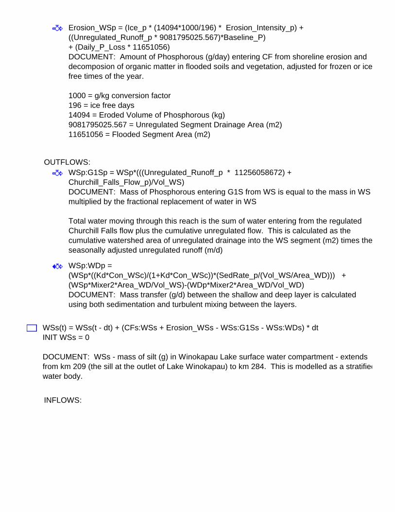
Erosion_WSp = (Ice_p * (14094*1000/196) * Erosion_Intensity_p) + ((Unregulated_Runoff_p * 9081795025.567)*Baseline_P)+ (Daily_P_Loss * 11651056)DOCUMENT: Amount of Phosphorous (g/day) entering CF from shoreline erosion and decomposion of organic matter in flooded soils and vegetation, adjusted for frozen or ice free times of the year.
1000 = g/kg conversion factor196 = ice free days14094 = Eroded Volume of Phosphorous (kg)9081795025.567 = Unregulated Segment Drainage Area (m2)11651056 = Flooded Segment Area (m2)
OUTFLOWS:WSp:G1Sp = WSp*(((Unregulated_Runoff_p * 11256058672) + Churchill_Falls_Flow_p)/Vol_WS)DOCUMENT: Mass of Phosphorous entering G1S from WS is equal to the mass in WS multiplied by the fractional replacement of water in WS
Total water moving through this reach is the sum of water entering from the regulated Churchill Falls flow plus the cumulative unregulated flow. This is calculated as the cumulative watershed area of unregulated drainage into the WS segment (m2) times the seasonally adjusted unregulated runoff (m/d)
WSp:WDp = (WSp*((Kd*Con_WSc)/(1+Kd*Con_WSc))*(SedRate_p/(Vol_WS/Area_WD))) + (WSp*Mixer2*Area_WD/Vol_WS)-(WDp*Mixer2*Area_WD/Vol_WD)DOCUMENT: Mass transfer (g/d) between the shallow and deep layer is calculated using both sedimentation and turbulent mixing between the layers.
WSs(t) = WSs(t - dt) + (CFs:WSs + Erosion_WSs - WSs:G1Ss - WSs:WDs) * dtINIT WSs = 0
DOCUMENT: WSs - mass of silt (g) in Winokapau Lake surface water compartment - extends from km 209 (the sill at the outlet of Lake Winokapau) to km 284. This is modelled as a stratified water body.
INFLOWS:
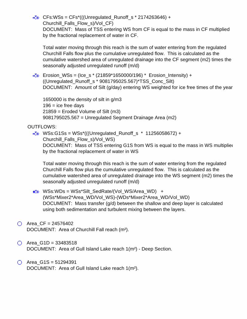
CFs:WSs = CFs*(((Unregulated_Runoff_s * 2174263646) + Churchill_Falls_Flow_s)/Vol_CF)DOCUMENT: Mass of TSS entering WS from CF is equal to the mass in CF multiplied by the fractional replacement of water in CF.
Total water moving through this reach is the sum of water entering from the regulated Churchill Falls flow plus the cumulative unregulated flow. This is calculated as the cumulative watershed area of unregulated drainage into the CF segment (m2) times the seasonally adjusted unregulated runoff (m/d)
Erosion_WSs = (Ice_s * (21859*1650000/196) * Erosion_Intensity) + ((Unregulated_Runoff_s * 9081795025.567)*TSS_Conc_Silt)DOCUMENT: Amount of Silt (g/day) entering WS weighted for ice free times of the year
1650000 is the density of silt in g/m3196 = ice free days21859 = Eroded Volume of Silt (m3)9081795025.567 = Unregulated Segment Drainage Area (m2)
OUTFLOWS:WSs:G1Ss = WSs*(((Unregulated_Runoff_s * 11256058672) + Churchill_Falls_Flow_s)/Vol_WS)DOCUMENT: Mass of TSS entering G1S from WS is equal to the mass in WS multiplied by the fractional replacement of water in WS
Total water moving through this reach is the sum of water entering from the regulated Churchill Falls flow plus the cumulative unregulated flow. This is calculated as the cumulative watershed area of unregulated drainage into the WS segment (m2) times the seasonally adjusted unregulated runoff (m/d)
WSs:WDs = WSs*Silt_SedRate/(Vol_WS/Area_WD) + (WSs*Mixer2*Area_WD/Vol_WS)-(WDs*Mixer2*Area_WD/Vol_WD)DOCUMENT: Mass transfer (g/d) between the shallow and deep layer is calculated using both sedimentation and turbulent mixing between the layers.
Area_CF = 24576402DOCUMENT: Area of Churchill Fall reach (m²).
Area_G1D = 33483518DOCUMENT: Area of Gull Island Lake reach 1(m²) - Deep Section.
Area_G1S = 51294391DOCUMENT: Area of Gull Island Lake reach 1(m²).

Area_G2D = 32525137DOCUMENT: Area of Gull Island Lake reach 2 (m²) - Deep Section.
Area_G2S = 48888848DOCUMENT: Area of Gull Island Lake reach 2 (m²).
Area_HV = 63823506DOCUMENT: Area of Happy Valley reach (m²).
Area_ML1 = 21689342DOCUMENT: Area of Muskrat Lake reach 1 (m²).
Area_ML2 = 28174787DOCUMENT: Area of Muskrat Lake reach 2 (m²).
Area_ML3 = 51060068DOCUMENT: Area of Muskrat Lake reach 3 (m²).
Area_WD = 51112985DOCUMENT: Area of Winokapau reach (m²) - Deep Section.
Area_WS = 88437872DOCUMENT: Area of Winokapau reach (m²).
Baseline_P = 0.01DOCUMENT: P_conc - the background phosphorus concentration in river water, is assumed to be 0.01 mg/L = 0.01 g/m3. This value is the approximate baseline concentration for the Churchill river, although significant deviations from this value are associated with high TSS concentrations and high flow during spring run off in the lower portion of the river.
Churchill_Falls_Flow_c = Churchill_Falls_Flow_sDOCUMENT: Churchill_Falls_Flow_c - flow of the Churchill River at Churchill Falls tailrace, based on the master variable Churchill_Falls_Flow_s.
Churchill_Falls_Flow_p = Churchill_Falls_Flow_sDOCUMENT: Churchill_Falls_Flow_p - flow of the Churchill River at Churchill Falls tailrace, based on the master variable Churchill_Falls_Flow_s.
Churchill_Falls_Flow_s = Churchill_Falls_Flow*WetmasterDOCUMENT: Churchill_Falls_Flow_s - seasonally variable flow rate of the Churchill River at the Churchill Falls tailrace, used to drive the silt submodel, with units of m3/day.

Clay_SedRate = 0.6*SettlemasterDOCUMENT: Clay_SedRate - particle settling rate (m/day) is the distace that a sinking particle will fall in one day. The model runs for two particle size classes, phi 4-6 representing silt and phi 7-9 representing clay. Unique particle settling velocities (m/day) are assigned to each phi class as follows: silt = 21 m/day; clay = 0.6 m/day.
ConD_CFp = (CFp / (1+Kd*Con_CFc))/Vol_CFDOCUMENT: All concentrations (variables beginning with "Con") will be expressed in units of g/m3.
ConD_G1Dp = (G1Dp / (1+Kd*Con_G1Dc))/Vol_G1DConD_G1Sp = (G1Sp / (1+Kd*Con_G1Sc))/Vol_G1SConD_G2Dp = (G2Dp / (1+Kd*Con_G2Dc))/Vol_G2DConD_G2Sp = (G2Sp / (1+Kd*Con_G2Sc))/Vol_G2SConD_HVp = (HVp / (1+Kd*Con_HVc))/Vol_HVConD_ML1p = (ML1p / (1+Kd*Con_ML1c))/Vol_ML1ConD_ML2p = (ML2p / (1+Kd*Con_ML2c))/Vol_ML2ConD_ML3p = (ML3p / (1+Kd*Con_ML3c))/Vol_ML3ConD_WDp = (WDp / (1+Kd*Con_WDc))/Vol_WDConD_WSp = (WSp / (1+Kd*Con_WSc))/Vol_WSConT_CFp = CFp/Vol_CFConT_G1Dp = G1Dp/Vol_G1DConT_G1Sp = G1Sp/Vol_G1SConT_G2Dp = G2Dp/Vol_G2DConT_G2Sp = G2Sp/Vol_G2SConT_HVp = HVp/Vol_HVConT_ML1p = ML1p/Vol_ML1ConT_ML2p = ML2p/Vol_ML2ConT_ML3p = ML3p/Vol_ML3ConT_WDp = WDp/Vol_WDConT_WSp = WSp/Vol_WSCon_CF = Con_CFs+Con_CFcCon_CFc = CFc/Vol_CFCon_CFs = CFs/Vol_CFCon_G1D = Con_G1Ds+Con_G1DcCon_G1Dc = G1Dc/Vol_G1DCon_G1Ds = G1Ds/Vol_G1DCon_G1S = Con_G1Ss+Con_G1ScCon_G1Sc = G1Sc/Vol_G1SCon_G1Ss = G1Ss/Vol_G1SCon_G2D = Con_G2Ds+Con_G2DcCon_G2Dc = G2Dc/Vol_G2DCon_G2Ds = G2Ds/Vol_G2D

Con_G2S = Con_G2Ss+Con_G2ScCon_G2Sc = G2Sc/Vol_G2SCon_G2Ss = G2Ss/Vol_G2SCon_HV = Con_HVs+Con_HVcCon_HVc = HVc/Vol_HVCon_HVs = HVs/Vol_HVCon_ML1 = Con_ML1s+Con_ML1cCon_ML1c = ML1c/Vol_ML1Con_ML1s = ML1s/Vol_ML1Con_ML2 = Con_ML2s+Con_ML2cCon_ML2c = ML2c/Vol_ML2Con_ML2s = ML2s/Vol_ML2Con_ML3 = Con_ML3s+Con_ML3cCon_ML3c = ML3c/Vol_ML3Con_ML3s = ML3s/Vol_ML3Con_WD = Con_WDs+Con_WDcCon_WDc = WDc/Vol_WDCon_WDs = WDs/Vol_WDCon_WS = Con_WSs+Con_WScCon_WSc = WSc/Vol_WSCon_WSs = WSs/Vol_WSDOCUMENT: All concentrations (variables beginning with "Con") will be expressed in units of g/m3.
Daily_P_Loss = Decay_C*((5220+8960)/200)DOCUMENT: Average carbon content from above ground vegetation is expected to be 5220 g/m². Average carbon content in forest floor litter/duff layer (0.1 m thick) is estimated to be 8960 g/m². Therefore the total soil and plant carbon content of flooded areas is 14180 g/m².
The soil and vegetation carbon to phosphorus molar ratio is assumed to be 500:1, and the atomic masses of carbon and phosphorous are 12 and 31 respectively, so the carbon to phosphorous mass ratio becomes 6000:31 or roughly 200:1.
Decaymaster = 1DOCUMENT: Decaymaster increases or decreases the rate of biomass decomposition. The default value is 1.0. Under enhanced decomposition, the value is 1.333; under low decomposition the value is 0.667.
Deposited_Clay = CFMc+G1Mc+G2Mc+HVMc+ML1Mc+ML2Mc+ML3Mc+WMcDeposited_P = CFMp+G1Mp+G2Mp+HVMp+ML1Mp+ML2Mp+ML3Mp+WMpDeposited_Silt = CFMs+G1Ms+G2Ms+HVMs+ML1Ms+ML2Ms+ML3Ms+WMs

Dispers = 162*MixmasterDOCUMENT: Dispers is a turbulent dispersive horizontal mixing coefficient. Horizontal dispersion coefficients (cm2/sec) depend on the scale of the phenomenon. Based on the assumption that the centres of the two deep water compartments (G1D and G2) are approximately 53 km (5.3E6 cm) apart, a horizontal dispersion coefficient of approximately 1E6 cm2/s is appropriate. This suggests a mean effictive horizontal water velocity across the boundary between the compartments of approximately 0.187 cm/s or 162 m/day. This value is probably accurate within an order of magnitude, or a factor of 3 higher or lower. Thus, bounding values of 486 m/day (fast mixing) and 54 m/day (slow mixing) are proposed. Variation in the value is achieved through the variable Mixmaster.
Erosion_Intensity_p = Erosion_IntensityDOCUMENT: Erosioin_Intensity_p - the rate at which phosphorus enters the water from shoreline soil erosion is the same rate used to model silt and clay entry into the water column.
Ice_c = Ice_sDOCUMENT: Ice_c - the ice free period used in modeling clay in water depends upon the master variable Ice_s.
Ice_p = Ice_cDOCUMENT: Ice_p - the ice free period used in modeling phosphorus in water depends upon the master variable Ice_s.
Julian = INT(1+(365*((TIME/365)-(INT(Time/365)))))DOCUMENT: Julian is a function that returns the "day of the year" as values ranging from 1 to 365, as the time of the simulation advances in total elapsed hours from the start of the simulation. This allows the Daily Runoff to recycle "year after year", based on a single hydrological year stored as a graph in that parameter.
Kd = 600 * 1e-6DOCUMENT: Kd - the water-sediment partition coefficient (m3/g) for Phosphorous on freshwater suspended sediment. Values in the literature range from approximately 10 to 1000 L/kg, the selected value is as follows:
Kd = 600 (L/kg) = 600 * (1 m3/1000 L)* (1 kg/1000g) = 600 * 1e-6 (m3/g)
Mixer2 = Mixer1*MixmasterDOCUMENT: Mixer2 - based on Mixer1, but adjusted for vertical mixing intensty by Mixmaster.
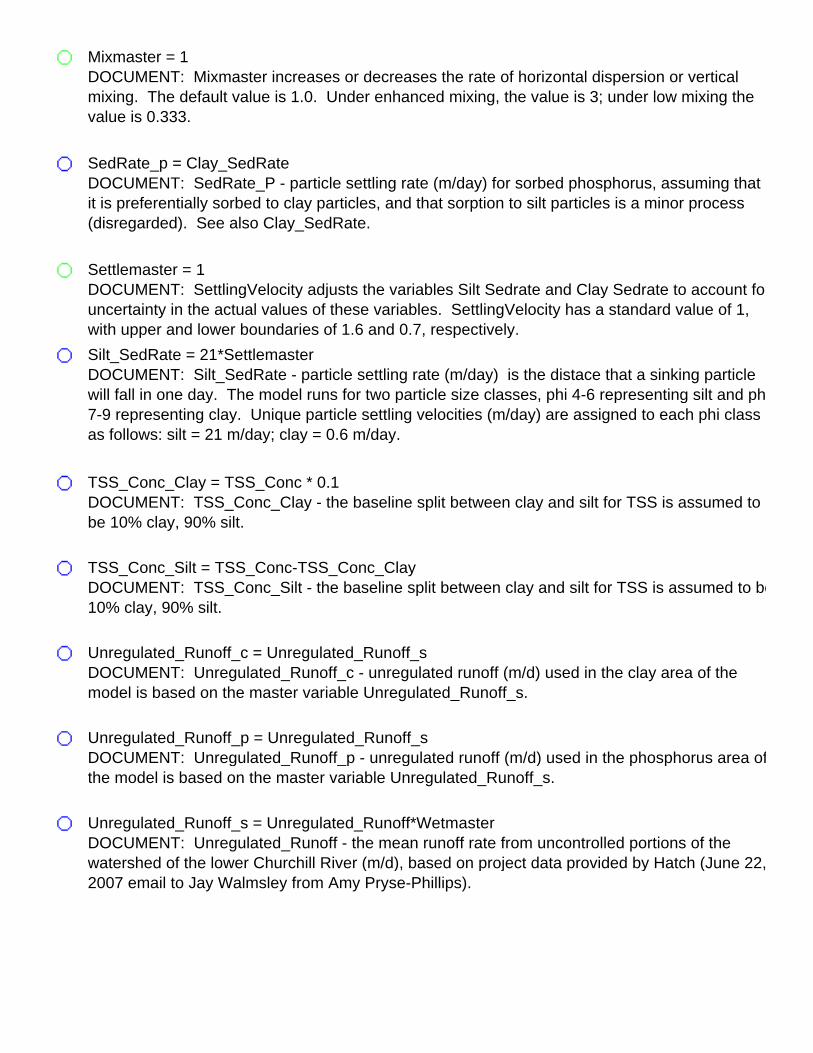
Mixmaster = 1DOCUMENT: Mixmaster increases or decreases the rate of horizontal dispersion or vertical mixing. The default value is 1.0. Under enhanced mixing, the value is 3; under low mixing the value is 0.333.
SedRate_p = Clay_SedRateDOCUMENT: SedRate_P - particle settling rate (m/day) for sorbed phosphorus, assuming that it is preferentially sorbed to clay particles, and that sorption to silt particles is a minor process (disregarded). See also Clay_SedRate.
Settlemaster = 1DOCUMENT: SettlingVelocity adjusts the variables Silt Sedrate and Clay Sedrate to account for uncertainty in the actual values of these variables. SettlingVelocity has a standard value of 1, with upper and lower boundaries of 1.6 and 0.7, respectively.
Silt_SedRate = 21*SettlemasterDOCUMENT: Silt_SedRate - particle settling rate (m/day) is the distace that a sinking particle will fall in one day. The model runs for two particle size classes, phi 4-6 representing silt and phi 7-9 representing clay. Unique particle settling velocities (m/day) are assigned to each phi class as follows: silt = 21 m/day; clay = 0.6 m/day.
TSS_Conc_Clay = TSS_Conc * 0.1DOCUMENT: TSS_Conc_Clay - the baseline split between clay and silt for TSS is assumed to be 10% clay, 90% silt.
TSS_Conc_Silt = TSS_Conc-TSS_Conc_ClayDOCUMENT: TSS_Conc_Silt - the baseline split between clay and silt for TSS is assumed to be 10% clay, 90% silt.
Unregulated_Runoff_c = Unregulated_Runoff_sDOCUMENT: Unregulated_Runoff_c - unregulated runoff (m/d) used in the clay area of the model is based on the master variable Unregulated_Runoff_s.
Unregulated_Runoff_p = Unregulated_Runoff_sDOCUMENT: Unregulated_Runoff_p - unregulated runoff (m/d) used in the phosphorus area of the model is based on the master variable Unregulated_Runoff_s.
Unregulated_Runoff_s = Unregulated_Runoff*WetmasterDOCUMENT: Unregulated_Runoff - the mean runoff rate from uncontrolled portions of the watershed of the lower Churchill River (m/d), based on project data provided by Hatch (June 22, 2007 email to Jay Walmsley from Amy Pryse-Phillips).

Vol_CF = 241468602DOCUMENT: Vol_CF - volume of the surface water compartment in the Churchill Falls reach (m3).
Vol_G1D = 933546005DOCUMENT: Vol_G1D - volume of Gull Lake reach 1 deep water compartment (m3).
Vol_G1S = 1322017253DOCUMENT: Vol_G1S - volume of Gull Lake reach 1 shallow water compartment (m3)****TO BE CONFIRMED****
Vol_G2D = 1232917646DOCUMENT: Vol_G2D - volume of the Gull Lake reach 2 deep water compartment (m3).
Vol_G2S = 985696308DOCUMENT: Vol_G2S - volume of the Gull Lake reach 2 shallow water compartment (m3).
Vol_HV = 135046668*2DOCUMENT: Vol_HV - volume of the Happy Valley reach surface water compartment (m3) is multiplied by 2 to avoid numerical instability (generated by rapid flushing of water in the compartment) while still allowing the model to run at a dt of 4/day. This makes no difference to the results.
Vol_ML1 = 381092553DOCUMENT: Vol_ML1 - volume of the Muskrat Lake reach 1 surface water compartment (m3).
Vol_ML2 = 424549674DOCUMENT: Vol_ML2 - volume of the Muskrat Lake reach 2 surface water compartment (m3).
Vol_ML3 = 900733511DOCUMENT: Vol_ML3 - volume of the Muskrat Lake reach 3 surface water compartment (m3).
Vol_WD = 5128435346DOCUMENT: Vol_WD - volume of the Winokapau Lake deep water compartment (m3).
Vol_WS = 11189342547DOCUMENT: Vol_WS - volume of the Winokapau Lake surface water compartment (m3).
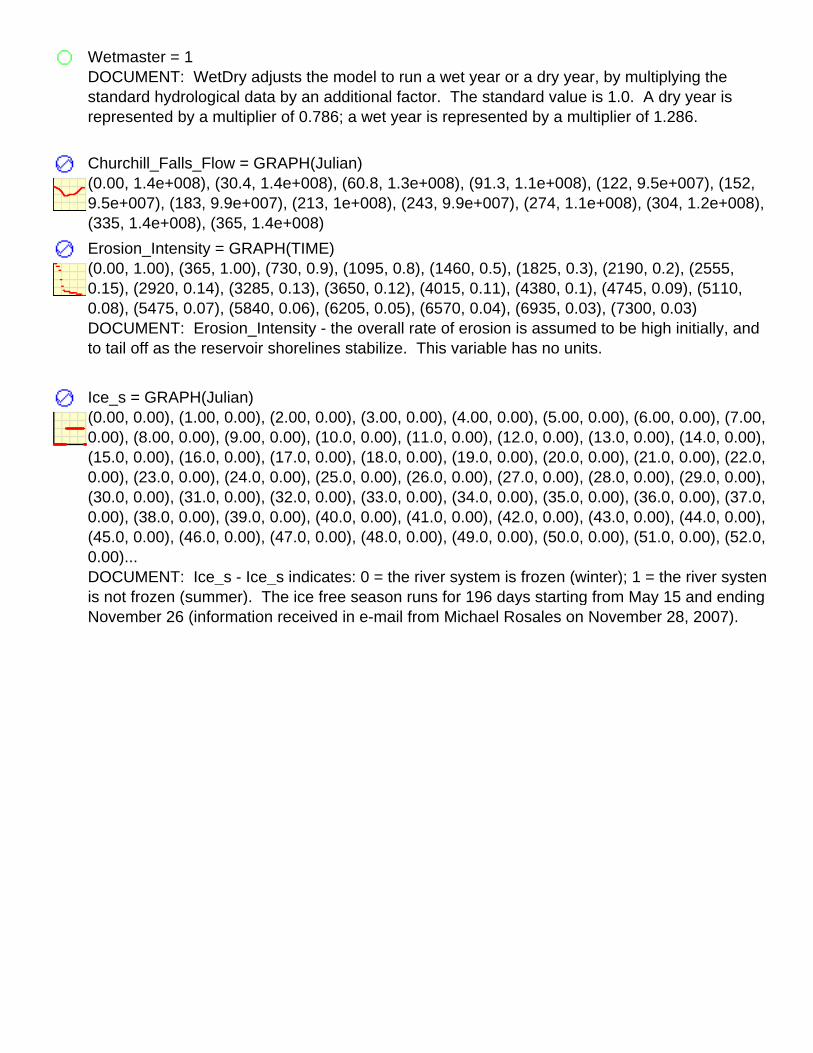
Wetmaster = 1DOCUMENT: WetDry adjusts the model to run a wet year or a dry year, by multiplying the standard hydrological data by an additional factor. The standard value is 1.0. A dry year is represented by a multiplier of 0.786; a wet year is represented by a multiplier of 1.286.
Churchill_Falls_Flow = GRAPH(Julian)(0.00, 1.4e+008), (30.4, 1.4e+008), (60.8, 1.3e+008), (91.3, 1.1e+008), (122, 9.5e+007), (152, 9.5e+007), (183, 9.9e+007), (213, 1e+008), (243, 9.9e+007), (274, 1.1e+008), (304, 1.2e+008), (335, 1.4e+008), (365, 1.4e+008)
Erosion_Intensity = GRAPH(TIME)(0.00, 1.00), (365, 1.00), (730, 0.9), (1095, 0.8), (1460, 0.5), (1825, 0.3), (2190, 0.2), (2555, 0.15), (2920, 0.14), (3285, 0.13), (3650, 0.12), (4015, 0.11), (4380, 0.1), (4745, 0.09), (5110, 0.08), (5475, 0.07), (5840, 0.06), (6205, 0.05), (6570, 0.04), (6935, 0.03), (7300, 0.03)DOCUMENT: Erosion_Intensity - the overall rate of erosion is assumed to be high initially, and to tail off as the reservoir shorelines stabilize. This variable has no units.
Ice_s = GRAPH(Julian)(0.00, 0.00), (1.00, 0.00), (2.00, 0.00), (3.00, 0.00), (4.00, 0.00), (5.00, 0.00), (6.00, 0.00), (7.00, 0.00), (8.00, 0.00), (9.00, 0.00), (10.0, 0.00), (11.0, 0.00), (12.0, 0.00), (13.0, 0.00), (14.0, 0.00), (15.0, 0.00), (16.0, 0.00), (17.0, 0.00), (18.0, 0.00), (19.0, 0.00), (20.0, 0.00), (21.0, 0.00), (22.0, 0.00), (23.0, 0.00), (24.0, 0.00), (25.0, 0.00), (26.0, 0.00), (27.0, 0.00), (28.0, 0.00), (29.0, 0.00), (30.0, 0.00), (31.0, 0.00), (32.0, 0.00), (33.0, 0.00), (34.0, 0.00), (35.0, 0.00), (36.0, 0.00), (37.0, 0.00), (38.0, 0.00), (39.0, 0.00), (40.0, 0.00), (41.0, 0.00), (42.0, 0.00), (43.0, 0.00), (44.0, 0.00), (45.0, 0.00), (46.0, 0.00), (47.0, 0.00), (48.0, 0.00), (49.0, 0.00), (50.0, 0.00), (51.0, 0.00), (52.0, 0.00)...DOCUMENT: Ice_s - Ice_s indicates: 0 = the river system is frozen (winter); 1 = the river system is not frozen (summer). The ice free season runs for 196 days starting from May 15 and ending November 26 (information received in e-mail from Michael Rosales on November 28, 2007).
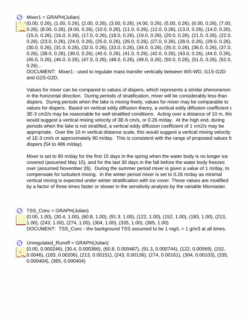
Mixer1 = GRAPH(Julian)(0.00, 0.26), (1.00, 0.26), (2.00, 0.26), (3.00, 0.26), (4.00, 0.26), (5.00, 0.26), (6.00, 0.26), (7.00, 0.26), (8.00, 0.26), (9.00, 0.26), (10.0, 0.26), (11.0, 0.26), (12.0, 0.26), (13.0, 0.26), (14.0, 0.26), (15.0, 0.26), (16.0, 0.26), (17.0, 0.26), (18.0, 0.26), (19.0, 0.26), (20.0, 0.26), (21.0, 0.26), (22.0, 0.26), (23.0, 0.26), (24.0, 0.26), (25.0, 0.26), (26.0, 0.26), (27.0, 0.26), (28.0, 0.26), (29.0, 0.26), (30.0, 0.26), (31.0, 0.26), (32.0, 0.26), (33.0, 0.26), (34.0, 0.26), (35.0, 0.26), (36.0, 0.26), (37.0, 0.26), (38.0, 0.26), (39.0, 0.26), (40.0, 0.26), (41.0, 0.26), (42.0, 0.26), (43.0, 0.26), (44.0, 0.26), (45.0, 0.26), (46.0, 0.26), (47.0, 0.26), (48.0, 0.26), (49.0, 0.26), (50.0, 0.26), (51.0, 0.26), (52.0, 0.26)...DOCUMENT: Mixer1 - used to regulate mass transfer vertically between WS-WD, G1S-G2D and G2S-G2D.
Values for mixer can be compared to values of dispers, which represents a similar phenonenon in the horizontal direction. During periods of stratification, mixer will be considerably less than dispers. During periods when the lake is mixing freely, values for mixer may be comparable to values for dispers. Based on vertical eddy diffusion theory, a vertical eddy diffusion coefficient of 3E-3 cm2/s may be reasonable for well stratified conditions. Acting over a distance of 10 m, this would suggest a vertical mixing velocity of 3E-6 cm/s, or 0.26 m/day. At the high end, during periods when the lake is not stratified, a vertical eddy diffusion coefficient of 1 cm2/s may be appropriate. Over the 10 m vertical distance scale, this would suggest a vertical mixing velocity of 1E-3 cm/s or approximately 90 m/day. This is consistent with the range of proposed values for dispers (54 to 486 m/day).
Mixer is set to 90 m/day for the first 15 days in the spring when the water body is no longer ice covered (assumed May 15), and for the last 30 days in the fall before the water body freezes over (assumed November 26). During the summer period mixer is given a value of 1 m/day, to compensate for turbulent mixing. In the winter period mixer is set to 0.26 m/day as minimal vertical mixing is expected under winter stratification with ice cover. These values are modified by a factor of three times faster or slower in the sensitivity analysis by the variable Mixmaster.
TSS_Conc = GRAPH(Julian)(0.00, 1.00), (30.4, 1.00), (60.8, 1.00), (91.3, 1.00), (122, 1.00), (152, 1.00), (183, 1.00), (213, 1.00), (243, 1.00), (274, 1.00), (304, 1.00), (335, 1.00), (365, 1.00)DOCUMENT: TSS_Conc - the background TSS assumed to be 1 mg/L = 1 g/m3 at all times.
Unregulated_Runoff = GRAPH(Julian)(0.00, 0.000246), (30.4, 0.000366), (60.8, 0.000487), (91.3, 0.000744), (122, 0.00569), (152, 0.0046), (183, 0.00206), (213, 0.00151), (243, 0.00136), (274, 0.00161), (304, 0.00103), (335, 0.000404), (365, 0.000404)