Advances in Pseudospectral Methods for Optimal Control

Advances in Pseudospectral Methods for Optimal

Control

Fariba Fahroo∗ and I. Michael Ross†

Recently, the Legendre pseudospectral (PS) method migrated from theory to flight ap-plication onboard the International Space Station for performing a finite-horizon, zero-propellant maneuver. A small technical modification to the Legendre PS method is neces-sary to manage the limiting conditions at infinity for infinite-horizon optimal control prob-lems. Motivated by these technicalities, the concept of primal-dual weighted interpolation,introduced earlier by the authors, is used to articulate a unified theory for all PS methodsfor optimal control. This theory illuminates the previously hidden fact of the unit weightfunction implicit in the the Legendre PS method based on Legendre-Gauss-Lobatto points.The unified framework also reveals why this Legendre PS method is the most appropriatemethod for solving finite-horizon optimal control problems with arbitrary boundary condi-tions. This conclusion is borne by a proper definition of orthogonality needed to generateconvergent approximations in Hilbert spaces. Special boundary conditions are needed toensure the convergence of the Legendre PS method based on the Legendre-Gauss-Radau(LGR) and the Legendre-Gauss (LG) points. These facts are illustrated by simple exam-ples and counter examples which reveal when and why PS methods based on LGR andLG points fail. A new kind of consistency in the primal-dual weight functions allows usto generate dual maps (such as Hamiltonians, adjoints etc) without resorting to solvingdifficult two-point boundary-value problems. These concepts are encapsulated in a unifiedCovector Mapping Theorem.

I. Introduction

In 2007, a front page article in SIAM News1 announced that pseudospectral optimal control was success-fully used to maneuver the International Space Station. Over the last decade, PS methods has moved rapidlyfrom theory and computation to ground experiments2,3 ... and now successful flight applications.1,4, 5 Therapid rise of PS methods is, in part, due to its independently reproducible superior performance when com-pared to other general purpose techniques.7–10 Furthermore, the versatility of PS methods is evident fromthe vast number of diverse optimal control problems that haven solved by various practitioners; examplesinclude space station attitude control,4,5 ascent guidance,7 interplanetary solar sail mission design,8 su-personic intercept,9,10 low-thrust Earth-to-Jupiter rendezvous,10 loitering of unmanned aerial vehicles,11,12

lunar guidance,13 libration-point stationkeeping,14 momentum-dumping,15 launch vehicle trajectory opti-mization,16 impulsive orbit transfer optimization,17 inert and electrodynamic tether control,18,19 magneticattitude control20 and many more.21 Solutions to well over a hundred problems are documented in Ref. [21].Many of the preceding example problems have been solved by OTIS22 and DIDO,23 the FORTRAN andMATLAB codes respectively for solving optimal control problems.

The most widely used PS method is the Legendre PS method24–26 that is based on the Legendre-Gauss-Lobatto (LGL) node points. This is simply because a rich number of convergence theorems have been provenin the literature,28–30 and hence one may use this method with a high degree of confidence in its validity. Inaddition, in practical applications, one may treat the outcome of the LGL/PS method in terms of a rigorousapplication of the Pontryagin Minimum Principle and accept or reject solutions based on the optimalityconditions.31 This comfort of guarantees is enunciated as the Covector Mapping Principle27,28,32–35 (CMP)which provides the foundations for generating explicit Covector Mapping Theorems.25,26,28,29 The proof

∗Professor, Department of Applied Mathematics, Naval Postgraduate School, Monterey, CA 93943. Email: [email protected] Fellow, AIAA

†Professor, Department of Mechanical & Astronautical Engineering, Code ME/Ro, Naval Postgraduate School, Monterey,CA 93943; [email protected]. Associate Fellow, AIAA.

1 of 23

American Institute of Aeronautics and Astronautics

SafeR

Text Box

AIAA Guidance, Navigation and Control Conference, Honolulu, HI, August 2008.

of this theorem utilizes specific quadrature formulas36,37 that have thus far shown to be valid only for theLGL/PS method, and hence the popularity of this approach.

In 2005, we proposed38 a PS method based on Legendre-Gauss-Radau (LGR) points to solve infinite-horizon optimal control problems. This proposal was motivated by a means to handle the singularity prob-lems that arise as a result of transforming the infinite-time domain to a finite time-domain. Additionalstudies showed39 a number of other advantages of the shifted LGR/PS method, particularly for real-timeapplications. This generates a natural question: does the LGR/PS method satisfy CMP-consistency? Anapparently simple way to investigate this issue is to apply the CMP to derive an explicit covector map34 ina manner similar to that of the LGL/PS approach. While conceptually simple, this task is not altogetherstraightforward as a key lemma related to an integration-by-parts formula26 is not readily available fornon-LGL methods. This crucial formula identifies the correct finite-dimensional inner-product space that isnecessary for the construction of the discretized 1-form that defines the sequences of discretized Lagrangiansthat converge to the continuous-time Lagrangian.40 In Ref. [41], we showed that a special weight functionmet all the appropriate criteria for the CMP leading to a new theorem on dual consistency for the LGR/PSmethod.

Motivated by these ideas for the LGR/PS method and their possible connections to the LGL/PS method,we develop a unified approach to investigate all PS methods. The key idea introduced in this paper is thenotion of weighed interpolants, their duals, and their direct effect on the generation of the correct pre-Hilbertspace where the computed solutions lie. The concept of a pre-Hilbert space is crucial for proofs of convergencetheorems28–30 that rely on the separability of the infinite-dimensional Hilbert spaces used to construct highly-accurate solutions to practical optimal control problems. We presented some of these ideas in Ref. [21]; here,we substantially expand and clarify our previous results.21

We begin this paper at the level of first principles by providing a unified set of foundations for all PSmethods for optimal control; i.e. PS methods over an arbitrary grid. In limiting the scope of the discussions,we focus on three Legendre PS methods: LGL, LGR and Legendre-Gauss (LG). From the perspective ofunification, it is shown that the LGL/PS method is indeed the correct Legendre PS method for solvingboundary value problems (BVPs) with arbitrary boundary conditions and hence all generic finite-horizonoptimal control problems. The unification also illustrates why the LGR/PS method is indeed better thanthe LGL/PS method for stabilizing control systems as this problem falls under the realm of a special optimalcontrol problem, the specialty being the infiniteness of the horizon. We illustrate some key consequences ofour theory by demonstrating how disastrous results are possible when the LGR/PS and LG/PS methodsare artificially forced to solve BVP-type problems over a finite horizon. Furthermore, in practical optimalcontrol problems, this disaster may be masked for low orders of discretization by giving the appearance ofconvergence;however, as the mesh is refined, the LGR and LG PS methods reveal a lack of convergence,particularly at the boundary points similar to the classic Runge phenomenon.42 Our theory explains thisphenomenon thus suggesting that the weighted-interpolant perspective is indeed the proper perspective forall PS methods for optimal control.

II. A Distilled Optimal Control Problem

For simplicity in exposition, we will consider the following scalar Bolza problem, with the understandingthat our discretization methods can be easily extended to higher-dimensional cases. For the same reasonwe will ignore path constraints as these can also be easily incorporated into our framework by replacing thecontrol Hamiltonian by the Lagrangian of the Hamiltonian.26 In simplifying such bookkeeping issues, weconsider the problem of finding the optimal state-control function pair t 7→ (x, u) ∈ R × R that solves thefollowing problem (Problem B):

x ∈ X ⊆ R, u ∈ R

(B)

Minimize J [x(·), u(·)] = E(x(−1), x(1)) +∫ 1

−1

F (x(t), u(t)) dt

Subject to x(t) = f(x(t), u(t))e(x(−1), x(1)) = 0

where X is an open set in R and the problem data (i.e. the endpoint cost function, E, the running costfunction, F , the vector field, f and the endpoint constraint function, e) are assumed to be at least C1-smooth.

2 of 23


An application of Pontryagin’s Minimum Principle (PMP) results in a two-point BVP that we denote asProblem Bλ. This “dualization” is achieved through the construction of the control Hamiltonian, H, andendpoint Lagrangian, E, defined as

H(λ, x, u) = F (x, u) + λf(x, u) (1)E(ν, x(−1), x(1)) = E(x(−1), x(1)) + νe(x(−1), x(1)) (2)

where λ is the adjoint covector (or costate) and ν is the endpoint covector. Problem Bλ is now posed asfollows:

(Bλ)

Find t 7→ (x, u, λ) and ν

Such that x(t)− f(x(t), u(t)) = 0e(x(−1), x(1)) = 0

λ(t) + ∂xH(λ(t), x(t), u(t)) = 0∂uH(λ(t), x(t), u(t)) = 0

λ(−1) +∂E

∂x(−1)(ν, x(−1), x(1)) = 0

λ(1)− ∂E

∂x(1)(ν, x(−1), x(1)) = 0

In using the PMP to solve a trajectory optimization problem, we must solve Problem Bλ which is clearly aproblem of finding the zeros of a map in an appropriate function space.43 This is the so-called indirect method.From a first-principles perspective,31 the PMP is used as follows: For every optimal solution to ProblemB, there exist an adjoint covector function, t 7→ λ, and an endpoint covector, ν, that satisfy the conditionsset forth by Problem Bλ. Thus, every candidate optimal solution to Problem B must also be a solutionto Problem Bλ under appropriate technical conditions. The LGL/PS method ensures a satisfaction of thiscondition through its Covector Mapping Theorem.25,26 A generalized and unified version of this theoremwith respect to PS methods is the main contribution of this paper and is developed in the following sections.A generalized version of this theorem with respect to the stability and convergence of the approximation isdescribed by Gong et al.28

III. A Unified Perspective on Pseudospectral Methods

The class of Legendre PS methods are a subset of a larger class of spectral methods which use orthogonalbasis functions in global expansions similar to Fourier and Sinc series expansions.44 What distinguishes PSmethods is that they are based on approximating the unknown functions by interpolants.45 This is one reasonwhy PS methods are sharply different from other polynomial methods previously considered in the literature.The interpolating points in a PS method can be any of the three major classes of Gaussian quadrature pointscalled nodes: Gauss points, Radau points and Lobatto points. Note that Radau and Lobatto points are alsoGaussian quadrature points; this is why specific PS methods are identified by adjectives that describe thespecific choice of nodes. All of these nodes are zeros of the orthogonal polynomials or their derivatives such asLegendre and Chebyshev or more generally the Jacobi polynomials. Thus, a very large family of PS methodscan be generated to solve optimal control problems. This notion is similar to Runge-Kutta (RK) methods.For example, Euler, trapezoid, Hermite-Simpson and many other methods are equivalently some form of anRK method with appropriately chosen coefficients.46 Just as not all RK methods are legitimate, not all PSmethods are legitimate. This is particularly true in solving optimal control problems as has been noted byHager.43 For example, an RK method that is legitimate for propagating an ODE may fail gloriously whenapplied to an optimal control problem. In other words, it is imperative to carefully select an appropriatemethod to solve optimal control problems.

In the absence of special information (such as special boundary conditions), it is customary to selectChebyshev PS methods in solving PDE problems as they are simple and effective. For optimal control ofODEs, the LGL/PS method is preferable as it maintains the consistency of dual approximations similar tothe Hager class of RK methods. Recently, we proposed the usage of Radau points38,39,41 as a means tomanage a singularity problem that arises in solving infinite-horizon control problems. The goal of this paperis to present a more unified view of these methods where we can show the similarities and differences of the

3 of 23


methods based on the choice of these different nodes and show the effect of these nodes on the discretizationof both the primal and dual problems.

A. Weighted Interpolants and Differentiation Matrices on Arbitrary Grids

We begin with the basic definition of PS methods and the different ingredients required in defining thesemethods for various nodes. Inspired by Weideman’s research,45 we select PS methods based on weightedinterpolants of the form,

y(t) ≈ yN (t) =N∑

j=0

W (t)W (tj)

φj(t)yj , a ≤ t ≤ b (3)

where y(t) is an arbitrary function. Here the nodes tj , j = 0, ..., N are a set of distinct interpolation nodes(defined below) in the interval [a, b], the weight function W (t) is a positive function on the interval, andφj(t) is the Nth− order Lagrange interpolating polynomial that satisfies the relationship φj(tk) = δjk. Thisimplies that

yj = yN (tj), j = 0, ...N. (4)

An expression for the Lagrange polynomial can be written as44

φj(t) =gN (t)

g′N (tj)(t− tj), gN (t) =

N∏

j=0

(t− tj). (5)

One important tenant of polynomial approximation of functions is that differentiation of the approximatedfunctions can be performed by differentiation of the interpolating polynomial,

dyN (t)dt

=N∑

j=0

yj

W (tj)[W ′(t)φj(t) + W (t)φ′j ]

Since only the values of the derivative at the nodes ti are required for PS methods, then we have,

dyN (t)dt

∣∣∣∣ti

=N∑

j=0

yj

W (tj)[W ′(ti)δij + W (ti)Dij ] =

N∑

j=0

Dij [W ]yj (6)

where we use Dij [W ] as a shorthand notation for the W -weighted differentiation matrix,

Dij [W ] :=[W ′(ti)δij + W (ti)Dij ]

W (tj)(7)

and Dij is usual unweighted differentiation matrix given by,

Dij :=dφj(t)

dt

∣∣∣∣t=ti

(8)

Thus, when W (t) = 1, we haveDij [1] = Dij (9)

From Eq. (5), the unweighted differentiation matrix, Dij = φ′j(ti), has the form,

Dij =

g′N (ti)g′N (tj)

1(ti − tj)

, i 6= j

g′′N (ti)2g′N (ti)

, i = j

(10)

The above equations are the general representations of the derivative of the Lagrange polynomials evaluatedat arbitrary interpolation nodes. Thanks to Runge, it is well-known that an improper selection of the gridpoints can lead to disastrous consequences. In fact, a uniform distribution of grid points is the worst possiblechoice for polynomial interpolation and hence differentiation. On the other hand, the best possible choice ofgrid points for integration, differentiation and interpolation of functions are Gaussian quadrature points.36

Consequently, all PS methods use Gaussian quadrature points. In order to limit the scope of this paper, welimit our discussions to Gaussian points based on Legendre polynomials as these polynomials offer eleganttheoretical properties for optimal control applications.

4 of 23


B. Legendre Nodes

Gaussian quadrature points lie in the interval [−1, 1]. In most problems the physical problem is posedon some interval [a, b] which can then be easily transformed to the computational domain [−1, 1] via alinear transformation. The Gauss quadrature points are zeros that are interior to the interval [−1, 1]. TheGauss-Radau zeros include one of the end points of the interval, usually the left-end point at t = −1.The Gauss-Lobatto points include both endpoints of the interval at t = −1, and t = 1; see Fig. 1. These

−1 −0.75 −0.5 0 0.5 0.75 1

Gauss

Gauss−Radau

Gauss−Lobatto

Figure 1. Illustrating the various Legendre quadrature nodes: Legendre-Gauss (LG), Legendre-Gauss-Radau (LGR) andLegendre-Gauss-Lobatto (LGL) grid points.

quadrature nodes are related to the zeros of the Qth-order Jacobi polynomials Pα,βQ which are orthogonal

on the interval [−1, 1] with respect to the inner product,36,37

∫ 1

−1

(1− t)α(1 + t)βPα,βQ (t)Pα,β

Q′ (t)dt (11)

Note that the Legendre polynomials are a special case of Jacobi polynomials which correspond to α = β = 0.Let tα,β

i,Q be the Q zeros of the Qth-order Jacobi polynomial Pα,βQ such that

Pα,βQ (tα,β

i,Q ) = 0, i = 0, ..., Q− 1 (12)

Then, we can define zeros and weights that approximate the following integral

∫ 1

−1

u(t)dt =N∑

i=0

wiu(ti) + R(u) (13)

and find expressions for the unweighted differentiation matrices for these nodes as follows:37

1. Legendre-Gauss (LG)

ti = t0,0i,N+1, i = 0, . . . , N

w0,0i =

21− (ti)2

[d

dt(LN+1(t)|t=ti

]−2

, i = 0, . . . , N,

R(u) = 0 if u(t) ∈ P2N+1([−1, 1]).

Dij =

{L′N+1(ti)

L′N+1(tj)(ti−tj), i 6= j, 0 ≤ i, j ≤ N

ti

1−ti2 , i = j

5 of 23


2. Legendre-Gauss-Radau (LGR)

ti =

{−1, i = 0,

t0,1i−1,N , i = 0, . . . , N

w0,0i =

1− ti(N + 1)2[LN (ti)]2

, i = 0, . . . , N,

R(u) = 0 if u(t) ∈ P2N ([−1, 1]).

Dij =

−N(N+2)4 , i = j = 0,

LN (ti)LN (tj)

1−tj

1−ti

1(ti−tj)

, i 6= j, 0 ≤ i, j ≤ N1

2(1−ti), 1 ≤ i = j ≤ N

3. Legendre-Gauss-Lobatto (LGL)

ti =

−1, i = 0,

t1,1i−1,N−1, i = 1, . . . , N − 1

1 i = 1

w0,0i =

2N(N + 1)[LN (ti)]2

, i = 0, . . . , N,

R(u) = 0 if u(t) ∈ P2N−1([−1, 1]).

Dij =

−N(N+1)4 , i = j = 0,

LN (ti)LN (tj)

1(ti−tj)

, i 6= j, 0 ≤ i, j ≤ N

0, 1 ≤ i = j ≤ N − 1N(N+1)

4 , i = j = N,

where PN is the set of all algebraic polynomials of degree at most N .

C. Pre-Hilbert Spaces

Given the definitions of the quadrature nodes and weights above, we can proceed with the definitions ofthe appropriate discrete inner-product spaces associated with the above nodes and weights. Let [−1, 1] 7→{y(t), z(t)} be real-valued functions in L2([−1, 1],R). The standard inner product in L2 is given by

〈y, z〉L2 :=∫ +1

−1

y(t)z(t) dt

For any given m ∈ N, and {wj > 0, j = 0, 1, . . . m}, define the weighted discrete inner product in L2 to be

〈y, z〉m,w :=m∑

j=0

y(tj)wjz(tj)

For the various Gauss quadrature nodes and the standard inner-product in L2, we have the following result:44

Lemma 1 For all pq ∈ P2N+ζ ,〈p, q〉L2 = 〈p, q〉N,w

where ζ = 1 for Legendre-Gauss (LG), ζ = 0 Legendre-Gauss-Radau (LGR) and ζ = −1 for Legendre-Gauss-Lobatto (LGL) integration and weights.

6 of 23


For any weight function, W (t), the weighted inner product in L2 is given by

〈y, z〉L2W

:=∫ +1

−1

y(t)W (t)z(t) dt

Let W (t) be any one of the following weight functions,

W (t) =

Wlgl(t) ⇒ W (t) = 1

Wlgr(t) ⇒ W (t) = 1− t

Wlg(t) ⇒ W (t) = 1− t2

(14)

From Lemma 1, we have the following unified result:

Lemma 2 For all pq ∈ P2N−1,〈p, q〉L2

W= 〈p, q〉N,w

Remark 1 Lemma 2 implies that Wlgl is the only weight function that is dual to itself in the standard innerproduct space and unweighted interpolation.

This primal-dual symmetry explains why the LGL PS method offers elegant properties.

Lemma 3 For the three Legendre quadrature nodes, LG, LGR and LGL, the following relationships hold:For i 6= j we have,

Dij = −W (tj)W (ti)

wj

wiDji

Hence, we can write,Dij [W ] = −wj

wiDji, i 6= j

and for i = j the following relationships hold:

For LG Nodes → Dii[Wlg] = −Dii, i = 0, · · · , N (15)

For LGR Nodes →{

Dii[Wlgr] = −Dii i = 1, · · · , N

D00[Wlgr] = −D00 − 1w0

(16)

For LGL Nodes →

Dii[Wlgl] = Dii = 0, i = 1, · · · , N − 1D00[Wlgl] = −D00 − 1/w0

DNN [Wlgl] = −DNN + 1/wN

(17)

IV. Primal-Dual Pseudospectral Discretizations

We can now define LG, LGR and LGL pseudospectral methods based on the choice of interpolationnodes. For approximating the state and costate variables we use the expansions,

xN (t) =N∑

j=0

W (t)W (tj)

xjφj(t), λN (t) =N∑

j=0

W ∗(t)W ∗(tj)

λjφj(t) (18)

where W and W ∗ are appropriate choices of weight functions. Lemma 2 suggests that if we take W (t) = 1and LGL nodes, then we must take W ∗(t) = 1 as well. This is in conformance with the standard theory.26 Itis clear that the use of Lemma 2 in the integration-by-parts argument proposed in Refs. [26,56], generalizesthe standard theory by suggesting that if we take W (t) = 1 and LGR nodes, then W ∗(t) = 1− t; likewise, forW (t) = 1 and LG nodes, W ∗(t) = 1− t2. Similarly, if we take W (t) = 1− t for LGR nodes, then W ∗(t) = 1etc.; thus,

(W ∗(t))∗ = W (t) (19)

That is, the dual of the dual is the original function.

7 of 23


For approximating the control variables, we take

uN (t) =N∑

j=0

ujψj(t) (20)

where ψj(t) is any interpolant. Note this key point that constitutes part of the unification principles28,30.That is uN (t) is not necessarily constructed as a Lagrange interpolating polynomial; rather, uN (t) is con-structed using any type of interpolation such as linear, cubic, spline etc. In previous versions, it was assumedthat uN (t) must be Lagrange interpolants leading to certain convergence questions with increase in N . Bychoosing uN (t) to be any interpolant, we retain the key elements of pseudospectral theory while allowingψj(t) to be chosen arbitrarily. This arbitrariness can then be exploited to further enhance the spectralconvergence property of PS methods by collecting information in between nodes through an application ofBellman’s Principle. Thus ψj becomes an abstract interpolant that may be selected based on optimizationprinciples. These ideas have been fully discussed by Ross et al.47

The preceding points illustrate how PS methods for optimal control have indeed evolved to a separateand distinct theory from those used to solve problems in fluid dynamics, the original source of ideas for PSmethods for optimal control. It is clear that this paper is part of these new foundations for PS methods foroptimal control.

A. Discretization of the Primal Problem (BN)

Based on these new ideas, we formulate PS methods for optimal control as follows: From Eqs. (6) and (18),it follows that the state derivative is approximated as,

dxN (t)dt

∣∣∣∣ti

=N∑

j=0

Dij [W ]xj (21)

Suppose we set W (t) ≡ 1 for the state variables for all Legendre PS methods. This automatically definesdual weight functions for costate interpolation. We may also set W (t) according to the appropriate class ofweighted interpolations in which case we would arrive at the corresponding duals. Choosing W (t) ≡ 1 for theprimal variables implies that the primal differentiation matrix, D[W ], is the standard differentiation matrix(Cf. Eq. (9)). Applying the quadrature rules for approximating the integral terms and using the appropriateform of the derivative matrix according to the choice of the nodes, we have the following expressions forProblem BN which is the discretized form of Problem B:

X ∈ RNn , U ∈ RNn

(BN )

Minimize JN [X, U ] = E(x0, xN ) +N∑

j=0

wjF (xj , uj)

Subject toN∑

j=0

Dijxj − f(xi, ui) = 0 i = 0, 1, . . . , N

e(x0, xN ) = 0

where X = [x0, x1, . . . , xNn ] and U = [u0, u1, . . . , uNn ].

B. Selection of a Proper Choice of PS Methods

Lemma 2 suggests the proper choice of an appropriate PS method for Problem BN . In many optimal controlproblems the endpoints are not totally free and are frequently constrained; that is, the endpoint function, e,is typically a function of both x(−1) and x(1). Then, according to Lemma 2, we must choose the LGL/PSmethod. Now suppose that we choose an LG or LGR PS method for such a problem. The motivation forthis selection may be based on Lemma 1 which suggests the apparently higher degree of approximation forLG and LGR nodes when compared to LGL nodes. That this is not true is best illustrated by a simple

8 of 23


counter example of Gong et al:30

x = (x, v) ∈ R2, u ∈ R

(P1)

Minimize J [x(·), u(·)] =∫ 1

0

v(t)u(t) dt

Subject to x(t) = v(t)v(t) = −v(t) + u(t)v(t) ≥ 0

0 ≤ u(t) ≤ 2(x(0), v(0)) = (0, 1)(x(1), v(1)) = (1, 1)

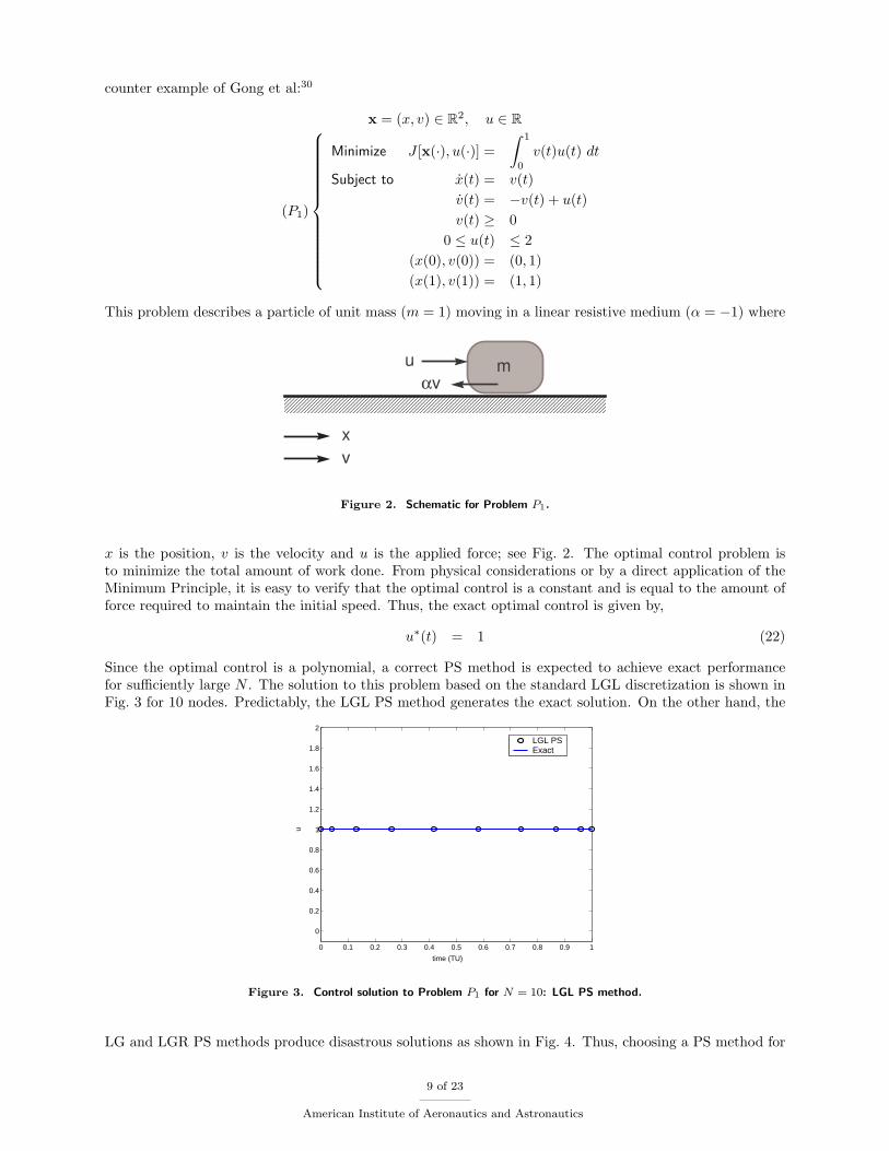
This problem describes a particle of unit mass (m = 1) moving in a linear resistive medium (α = −1) where

xxxxxxxxxxxxxxxxxxxxxxxxxxxxxxxxxxxxxxxxxxxxxxxxxxxxxxxxxxxxxxxxxxxxxxxxxxxxxxxxxxxxxxxxxxxxxxxxxxxxxxxxxxxxxxxxxxxxxxxxxxxxxxxxxxxxxxxxxxxxxxxxxxxxxxxxxxxxxxxxxxxxxxxxxxxxxxxxxxxxxxxxxxxxxxxxxxxxxxxxxxxxxxxxxxxxxxxxxxxxxxxxxxxxxxxxxxxxxxxxxxxxxxxxxxxxxxxxxxxxxxxxxxxxxxxxxxxxxxxxxxxxxxxxxxxxxxxxxxxxxxxxxxxxxxxxxxxxxxxxxxxxxxxxxxxxxxxxxxxxxxxxxxxxxxxxxxxxxxxxxxxxxxxxxxxxxxxxxxxxxxxxxxxxxxxxxxxxxxxxxxxxxxxxxxxxxxxxxxxxxxxxxxxxxxxxxxxxxxxxxxxxxxxxxxxxxxxxxxxxxxxxxxxxxxxxxxxxxxxxxxxxxxxxxxxxxxxxxxxxxxxxxxxxxxxxxxxxxxxxxxxxxxxxxxxxxxxxxxxxxxxxxxxxxxxxxxxxxxxxxxxxxxxxxxxxxxxxxxxxxxxxxxxxxxxxxxxxxxxxxxxxxxxxxxxxxxxxxxxxxxxxxxxxxxxxxxxxxxxxxxxx

xxxxxxxxxxx

xxxxxxxxxxx

x

v

xxxxxxxxxxxu

xxxxxxxxxx αv

m

Figure 2. Schematic for Problem P1.

x is the position, v is the velocity and u is the applied force; see Fig. 2. The optimal control problem isto minimize the total amount of work done. From physical considerations or by a direct application of theMinimum Principle, it is easy to verify that the optimal control is a constant and is equal to the amount offorce required to maintain the initial speed. Thus, the exact optimal control is given by,

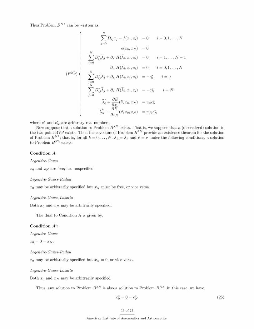
u∗(t) = 1 (22)

Since the optimal control is a polynomial, a correct PS method is expected to achieve exact performancefor sufficiently large N . The solution to this problem based on the standard LGL discretization is shown inFig. 3 for 10 nodes. Predictably, the LGL PS method generates the exact solution. On the other hand, the

0 0.1 0.2 0.3 0.4 0.5 0.6 0.7 0.8 0.9 1

0

0.2

0.4

0.6

0.8

1

1.2

1.4

1.6

1.8

2

time (TU)

u

LGL PSExact

Figure 3. Control solution to Problem P1 for N = 10: LGL PS method.

LG and LGR PS methods produce disastrous solutions as shown in Fig. 4. Thus, choosing a PS method for

9 of 23


0 0.1 0.2 0.3 0.4 0.5 0.6 0.7 0.8 0.9 1

0

0.2

0.4

0.6

0.8

1

1.2

1.4

1.6

1.8

2

u

time (TU)

LG PSExact

0 0.1 0.2 0.3 0.4 0.5 0.6 0.7 0.8 0.9 1

0

0.2

0.4

0.6

0.8

1

1.2

1.4

1.6

1.8

2

u

time (TU)

LGR PSExact

Figure 4. Control solutions to Problem P1 for N = 10: LGR and LG PS methods; compare Fig. 3.

optimal control based on Lemma 1 alone is a bad proposition. To illustrate the point that the LG and LGRPS methods are not just converging at a slower rate than the LGL PS method, their control solutions areplotted in Fig. 5 for N = 30. It is clear that the LG and LGR PS methods do not converge. What is most

0 0.1 0.2 0.3 0.4 0.5 0.6 0.7 0.8 0.9 1

0

0.2

0.4

0.6

0.8

1

1.2

1.4

1.6

1.8

2

u

time (TU)

LG PSExact

0 0.1 0.2 0.3 0.4 0.5 0.6 0.7 0.8 0.9 1

0

0.2

0.4

0.6

0.8

1

1.2

1.4

1.6

1.8

2u

time (TU)

LGR PSExact

Figure 5. Control solutions to Problem P1 for N = 30: Illustrating why the LGR and LG PS methods are the wrong PS methodsfor this problem.

interesting about the lack of convergence of the LGR and LG PS methods is that their node points convergeto the node points of the LGL PS method as N increases. This point is illustrated in Fig. 6.

C. Discretization of the Dualized Problem (BλN)

Given that dual space considerations are indeed important even when only primal variables are sought,34,43

we now explore the discretization of the dualized problem. From Eqs. (7) and (18), it follows that the costatederivative is approximated as,

dλN (t)dt

∣∣∣∣ti

=N∑

j=0

D∗ijλj (23)

with

D∗ij = Dij [W ] =

[W ′(ti)δij + W (ti)Dij ]W (tj)

10 of 23


−1 −0.75 −0.5 0 0.5 0.75 1

LG

LGR

LGL

Figure 6. Illustrating the near absence of differences between the three Legendre quadrature nodes for increasing N .

Thus Problem BλN which is the discretization of Problem Bλ defined in Sec. II, can be constructed as,

(BλN )

N∑

j=0

Dijxj − f(xi, ui) = 0 i = 0, 1, . . . , N

e(x0, xN ) = 0N∑

j=0

D∗ijλj + ∂xiH(λi, xi, ui) = 0 i = 0, 1, . . . , N

∂uiH(λi, xi, ui) = 0 i = 0, 1, . . . , N

λ0 +∂E

∂x0(ν, x0, xN ) = 0

λN − ∂E

∂xN(ν, x0, xN ) = 0

Thus, in the unified PS method, we use the matrices D and D∗ as primal and dual differentiation matricesarising from the primal and dual weighted interpolation with weight functions, W (t) and W ∗(t), respectively.Furthermore, from Eq. (19), it follows that we may choose W (t) for discretizing the dual, in which case weneed to use W ∗(t) for discretizing the primals.

V. A Unified Covector Mapping Theorem

Based on the preceding discussions it is now abundantly clear that the correct inner product space forall three PS discretizations is given by RNn

w , the finite-dimensional Hilbert space RNn equipped with theweighted inner product,

〈a, b〉RNnw

:=N∑

i=0

aiwibi a, b ∈ RNn

Thus, the Lagrangian in RNnw is given by,40

JN [λ, ν, x, u] =N∑

j=0

wjF (xj , uj) +N∑

i=0

wiλif(xi, ui)−N∑

i=0

wiλi

N∑

j=0

Dijxj + νe(x0, xN ) + E(x0, xN )

=N∑

i=0

wiH(λi, xi, ui)−N∑

i=0

wiλi

N∑

j=0

Dijxj + E(ν, x0, xN )

11 of 23


where λ and ν are the Karush-Kuhn-Tucker (KKT) multipliers in RNnw . From the KKT theorem we have,

∂xkJN [λ, ν, x, u] = wk∂xk

H(λk, xk, uk)−N∑

i=0

wiλi

N∑

j=0

Dijδjk k = 1, . . . , N − 1

= wk∂xkH(λk, xk, uk)−

N∑

i=0

wiλiDik

From Lemma 3 we have,

D∗ki := −wi

wkDik for k = 1, . . . , N − 1, i = 0, . . . , N (24)

Hence,

∂xkJN [λ, ν, X, U ] = wk

(∂xk

H(λk, xk, uk) +N∑

i=0

D∗kiλi

)= 0

Similarly,

∂xkJN [λ, ν, X, U ] = wk∂xk

H(λk, xk, uk)−N∑

i=0

wiλi

N∑

j=0

Dijδjk + ν∂xke(x0, xN ) k = 0, N

= wk∂xkH(λk, xk, uk)−

N∑

i=0

wiλiDik + ν∂xke(x0, xN )

From Lemma 3, this implies,


(∂xk


i=0

D∗kiλi

)+ λ

∗k + ν∂xk

e(x0, xN ) = 0, k = 0


(∂xk


i=0

D∗kiλi

)+ λ

∗k − ν∂xk

e(x0, xN ) = 0, k = N

where λ∗k is given by:

1. Legendre-Gauss

λ∗k = 0 for k = 0 and N

2. Legendre-Gauss-Radau

λ∗k = λk for k = 0 and λ

∗k = 0 for k = N

3. Legendre-Gauss-Lobatto

λ∗k = λk for k = 0 and N

12 of 23


Thus Problem BNλ can be written as,

(BNλ)

N∑

j=0

Dijxj − f(xi, ui) = 0 i = 0, 1, . . . , N

e(x0, xN ) = 0N∑

j=0

D∗ij λj + ∂xi

H(λi, xi, ui) = 0 i = 1, . . . , N − 1

∂uiH(λi, xi, ui) = 0 i = 0, 1, . . . , NN∑

j=0

D∗ij λj + ∂xi

H(λi, xi, ui) = −c∗0 i = 0

N∑

j=0

D∗ij λj + ∂xiH(λi, xi, ui) = −c∗N i = N

λ∗0 +

∂E

∂x0(ν, x0, xN ) = w0c

∗0

λ∗N − ∂E

∂xN(ν, x0, xN ) = wNc∗N

where c∗0 and c∗N are arbitrary real numbers.Now suppose that a solution to Problem BλN exists. That is, we suppose that a (discretized) solution to

the two-point BVP exists. Then the covectors of Problem BλN provide an existence theorem for the solutionof Problem BNλ; that is, for all k = 0, . . . , N , λk = λk and ν = ν under the following conditions, a solutionto Problem BNλ exists:

Condition A:

Legendre-Gauss

x0 and xN are free; i.e. unspecified.

Legendre-Gauss-Radau

x0 may be arbitrarily specified but xN must be free, or vice versa.

Legendre-Gauss-Lobatto

Both x0 and xN may be arbitrarily specified.

The dual to Condition A is given by,

Condition A∗:

Legendre-Gauss

x0 = 0 = xN .

Legendre-Gauss-Radau

x0 may be arbitrarily specified but xN = 0, or vice versa.

Legendre-Gauss-Lobatto

Both x0 and xN may be arbitrarily specified.

Thus, any solution to Problem BλN is also a solution to Problem BNλ; in this case, we have,

c∗0 = 0 = c∗N (25)

13 of 23


That is, Eq. (25) is a matching condition that matches Problem BNλ to Problem BλN . Matching condi-tions48,49 are part of the totality of closure conditions required to complete the circuit (arrows) indicated inFig. 7.

Note that Problems BN and BλN are generated from Problems B and Bλ respectively without introducingany additional continuous-time primal conditions to carry over to the discrete-time problems. This notion isimplicit in Fig. 7. Fig. 7 is a commutative diagram promulgated in Ref. [27] that forms part of the broader

Problem B

Problem B λ Problem B λN

Problem B N

du

aliz

atio

n

du

aliz

atio

n

approximation(direct method)

approximation(indirect method)

convergence

convergence

CovectorMappingTheorem

Problem B Nλ

shortest pathfor solvingProblem B

Figure 7. Illustrating the Covector Mapping Principle and the unification of direct and indirect methods inoptimal control as first described by Ross and Fahroo.25–27

notion of the Covector Mapping Principle in optimal control. A historical account of the origins of thisdiagram and the ideas embedded in it are documented in Ref. [33]. The concepts embedded in Fig. 7 formyet another unification principle in PS methods and optimal control at large.

A. A Unified Pseudospectral Covector Mapping Theorem

In completing the steps suggested in Fig. 7 towards the development of a Unified Covector Mapping Theorem,we identify the following multiplier sets analogous to those introduced in Ref. [50]: Let χ := {[xk], [uk]} andΛ := {ν0, [µk], [λk]}. We denote by MλN (χ) the multiplier set corresponding to χ,

MλN (χ) :={Λ : Λ satisfies conditions of Problem BλN

}(26)

Similarly, we define, Λ :={

ν0, [µk], [λk]}

and MNλ(χ) the multiplier set,

MNλ(χ) :={

Λ : Λ satisfies conditions of Problem BNλ}

(27)

Clearly, MλN (χ) ⊆MNλ(χ). We now define a new multiplier set,

MNλ(χ) :={

Λ ∈MNλ(χ) : Λ satisfies Eq. (25)}

(28)

Thus, MNλ(χ) ∼MλN (χ). That is, under a matching (closure) condition, every solution of Problem BNλ isalso a solution to Problem BλN . This statement is encapsulated as the Covector Mapping Theorem:

Theorem 1 (Unified Covector Mapping Theorem) Let MλN (χ) 6= ∅ and{

ν0, [µk], [λk]}∈ MNλ(χ);

then, the bijection, MNλ(χ) ∼MλN (χ), is given by,

λN (tk) = λk µN (tk) = µk, ν0 = ν0 (29)

Remark 2 The statement of Theorem 1 is identical to that of Ref. [50] and is made possible through theconstruction of weighted interpolation. The weighted interpolants lead to a consistent pair of differentiationmatrices, D and D∗, that are dual to each other. In this context, the LGL case turns out to be the specialsituation where the formal adjoint of D is the same as −D.

14 of 23


Remark 3 Note that Theorem 1 neither states λN (tk) = λk, µN (tk) = µk, ν0 = ν0 nor does it implyλN (tk) ≈ λk, µN (tk) ≈ µk, ν0 ≈ ν0 as is sometimes erroneously interpreted. Furthermore, note thatEq. (29) is an exact relationship.

Remark 4 A simple counter example is constructed in Ref. [33] to show that a solution to Problem BλN

may not exist for Euler discretization no matter how small the mesh. This well-known phenomenon requiresa proper technical modification to Theorem 1 similar to Polak’s theory of consistent approximations. Thisaspect of Theorem 1 is rigorously proved in Refs. [30] and [28] for unit weight functions. The extension ofthis rigor to non-unit weight function is straightforward but lengthy. Thus, the main assumption in Theorem1 that the multiplier set, MλN (χ), is non empty can be eliminated. In other words, Theorem 1 remains validunder much weaker assumptions.

Remark 5 Because the set MNλ(χ) is “larger” (i.e. has more elements) than MλN (χ), it de-sensitizes thesensitivities associated with solving Problem BN . This fact is exploited in Ref. [52] to design a “guess-free”algorithm for solving Problem B.

B. Some Remarks on the Covector Mapping Principle

The Covector Mapping Theorem was generated by an application of the Covector Mapping Principle (seeFig. 7). Since the introduction of Pontryagin’s Principle, it has been known that the Minimum Principlemay fail in the discrete-time domain if it is applied in exactly the same manner as in the continuous-timedomain. For the Minimum Principle to hold exactly in the discrete-time domain, additional assumptions ofconvexity are required whereas no such assumptions are necessary for the continuous-time versions. This isbecause the continuous-time problem has a hidden convexity49 that is implicitly used in proving theorems.Thus, when a continuous-time optimal control problem is discretized, this hidden convexity is not carriedover to the discrete time domain resulting in a loss of information. If this information loss is not restored, thediscrete-time solution may be spurious, not converge to the correct solution, or may even provide completelyfalse results. A historical account of these issues, along with a simple counter example, is described inRef. [33]. Further details are provided in the references contained in Ref. [33]. A thorough discussion ofthese issues and their relationship to advance concepts in optimal control theory has been developed byMordukhovich.48,49

The closure conditions introduced by Ross and Fahroo26 are a form of matching conditions that aresimilar in spirit to Mordukhovich’s matching conditions for Euler approximations. These conditions can bein primal space alone,48,51 or in primal-dual space.34 Note however that the primal space conditions48,51

are obtained through dual space considerations. These new ideas reveal that dual space issues cannot beignored even in the so-called “direct methods,” for optimal control.

C. Software

A proper implementation of a PS method requires addressing all the numerical stability and accuracy issuesand a case-by case approach to problem solving using PS approximations is inadvisable as it is tantamountto using first principles in every situation. Consequently, it is preferable for all the intricacies of a PSmethod to be implemented just once for a general problem in a form of a reusable software package. Thisexercise has been carried out in both OTIS and DIDO.23 OTIS is in FORTRAN while DIDO is in MATLAB.While OTIS uses PS techniques an one of its many option, DIDO is exclusively based on PS methods alone.In addition, DIDO implements the spectral algorithm53 to complete the “circuit” shown in Fig. 7. Thegeneralized approach is implemented in an α-version of the software package. This software was used in thefollowing sections that illustrate the principles and practice.

VI. Illustrative Some Key Points of the Main Theorem

In this section we will illustrate the many elements of our unified theory. From the statements of Theorem1, it is clear that the LGL PS method is the most general of the Legendre PS methods and is hence applicableto all finite-horizon optimal control problems. Furthermore, note that although the Covector MappingTheorem is meaningful only under convergence of the discretization, convergence issues are separate anddistinct concepts. The apparently many nuances of the Unified Covector Mapping Theorem can be bestillustrated by examples and counter examples.

15 of 23


A. Convergence of the Costates Does Not Imply Convergence of the Control

Obviously, the key variable in an optimal control problem is the control variable. Thus, convergence of thecontrol variable implies convergence of the states and costates under fairly mild conditions; however, theopposite is not true.54 To illustrate this point we once again consider Problem P1. By a direct applicationof the Minimum Principle, it can be shown that the exact values of the costates are given by,

λx(t) = −2 (30)λv(t) = −1 (31)

Figure 3 shows that the LGL controls have converged; thus, as expected, the LGL costates converge asillustrated in Fig. 8. On the other hand, the controls for the LG and LGR PS methods do not converge (see

0 0.1 0.2 0.3 0.4 0.5 0.6 0.7 0.8 0.9 1−2

−1.8

−1.6

−1.4

−1.2

−1

−0.8

−0.6

cost

ates

−LG

L

Time (TU)

Figure 8. Exact and LGL PS costates for Problem P1.

Fig. 5) despite that the costates do indeed converge as illustrated in Fig. 9.

0 0.1 0.2 0.3 0.4 0.5 0.6 0.7 0.8 0.9 1−2.2

−2

−1.8

−1.6

−1.4

−1.2

−1

−0.8

cost

ates

−G

auss

Time (TU)0 0.1 0.2 0.3 0.4 0.5 0.6 0.7 0.8 0.9 1

−2.2

−2

−1.8

−1.6

−1.4

−1.2

−1

−0.8

cost

ates

−LG

R

Time (TU)

Figure 9. Exact and PS costates for Problem P1: LG and LGR PS methods; compare Fig. 5.

B. Illustrating the Utility of the Covector Mapping Theorem

The premise of computational methods is that, unlike Problem P1 most optimal control problems do nothave analytical solutions. Consequently, any computational solution requires theoretical justification alongwith multiple and independent means to verify feasibility and optimality of the solution. The CovectorMapping Theorem, when applied correctly, provides one such test. To illustrate this point, we consider themuch-studied orbit transfer problem of Moyer and Pinkham.55 This widely-studied31,51,56 classical problem,

16 of 23


has no analytical solution, and is given by,

x = (r, θ, vr, vt) ∈ R4, u = β ∈ R

(P2)

Minimize J [x(·),u(·)] = −r(tf )Subject to r(t) = vr(t)

θ(t) = vθ

r

vr(t) = v2θ

r − 1r2(t) + A(t) sin β(t)

vθ(t) = −vr(t)vθ(t)r(t) + A(t) cos β(t)

tf = 3.32(r(0), θ(0)) = (1, 0)

(vr(0), vθ(0)) = (0, 1)(vr(tf ), vθ(tf )) = (0,

√1/r(tf ))

where the state variables are the radial distance r, the angular distance θ, the radial velocity component vr,and the transverse velocity component vθ. The control variable is the thrust steering angle measured fromthe local horizontal β, and A(t) is the continuous acceleration parameterized by,

A(t) =T

(m0 − |m|t) (32)

where T = 0.1405, is the continuous thrust, m0 = 1.0 is the initial mass, and |m| = 0.0749 is the constantfuel consumption rate.

The state and control solution to this problem using the LGL PS method is shown in Fig. 10. Although,

0 0.5 1 1.5 2 2.5 3 3.50

0.5

1

1.5

2

2.5optimal states−LGL

optim

al s

tate

s

Time (TU)

r

θv

r

vθ

0 0.5 1 1.5 2 2.5 3 3.5−4

−3

−2

−1

0

1

2

3

optim

al c

ontr

ol−

LGL

Time (TU)

Figure 10. State and control trajectories for the LGL PS method.

this solution is identical to the validated one we obtained in Ref. [57] nearly a decade ago, one of theadvantages of the Covector Mapping Theorem is that it provides an independent means to test the optimalityof the solution by an application of Pontrygain’s Principle. To demonstrate this point, we begin by developingthe necessary conditions for Problem P2. It is straightforward to show that the adjoint equation for λθ alongwith the transversality condition indicates that,

λθ(t) = 0 (33)

The costates obtained by an application of the Covector Mapping Theorem are shown in Fig. 11. Clearly,Fig. 11 shows that λθ(t) = 0 to within numerical errors. Thus, it is clear that the Covector MappingTheorem is extremely useful in verifying the optimality of the candidate solution by a direct application ofPontryagin’s Principle.

17 of 23


0 0.5 1 1.5 2 2.5 3 3.5−2.5

−2

−1.5

−1

−0.5

0

0.5

1

1.5

cost

ates

−LG

LTime (TU)

λr

λθ

λv

r

λv

θ

Figure 11. The costate, t 7→ λθ, obtained from the Covector Mapping Theorem.

C. Illustrating The Multiplier Sets of Theorem 1

The concept of multiplier sets used in the statement of Theorem 1 is based on our prior work presented inRef. [50]. At this point it is useful to illustrate how our multiplier sets can be used while drawing attentionto their possible misuse as well.

It can be shown29 that for Problem P2, the map, χ ⇒ MNλ(χ), is indeed multivalued, and hence thenotation, ⇒. Let Λ ∈ MNλ(χ). Fig. 12 shows the multiplier trajectories obtained by one selection of the

0 0.5 1 1.5 2 2.5 3 3.5−0.35

−0.3

−0.25

−0.2

−0.15

−0.1

−0.05

0

0.05

0.1

0.15

KK

T M

ultip

liers

Time (TU)

Figure 12. KKT multiplier trajectories, t 7→ eλ, in the wrong Hilbert space and wrong selection.

set-valued map, MNλ(χ). This selection is based on a least-squares solution (LSQ) of minimizing∥∥∥Λ

∥∥∥2,

(LSQ)

Minimize∥∥∥Λ

∥∥∥2

2

Subject to Λ ∈MNλ(χ)

Comparing Figs. 11 and 12, it is clear that the multiplier trajectories of Fig. 12 are not the discrete costates;they are not even approximations as noted in Remark 3. Because the dual space is a weighted Hilbert space,one could credibly argue that the multiplier trajectories of Fig. 12 are in the wrong space. By selecting themultipliers in the correct Hilbert space but still based on the selection given by Problem LSQ, we get themultiplier trajectories shown in Fig. 13. Clearly, none of the KKT multipliers can be construed as discretecostate trajectories. The correct selection of multiplier trajectories are indeed obtained from Eq. (28). Notsurprisingly, a proper use of the theory generates the right answer!

18 of 23


0 0.5 1 1.5 2 2.5 3 3.5−6

−4

−2

0

2

4

6

8

KK

T M

ultip

liers

Time (TU)

Figure 13. KKT multiplier trajectories, t 7→ eλ, in the correct Hilbert space but wrong selection.

As a final point of contention we note that it is incorrect to interpret any of the KKT multiplier trajectoriesas “wiggles” about the correct answer. The appearance of the wiggles is simply a result of existence of aprimal solution in the absence of satisfying the KKT constraint qualifications. A proof of this assertion isbeyond the scope of this paper but may be found in Refs. [25, 26, 28, 32–35, 40, 58] with various levels ofsophistication and rigor.

Based on the primal space arguments put forth in Sec V.B, it is clear that the LGR and LG PS methodsare inappropriate for Problem P2 as well. Nonetheless, it is instructive to explore the consequences ofselecting the wrong PS method, and examine its dual space consequences.

D. Illustrating the Consequences of an Improper Choice of a PS Method

From Theorem 1, it is clear that we should not use the LGR or LG PS methods for this problem. Regardless,it is instructive to examine their numerical performance in order to determine the practical consequences ofchoosing the wrong PS method. As already noted previously, what matters in optimal control problems isthe convergence of the control variables; hence, we focus our attention on the convergence of the control.

The optimal controls for the LGR PS method is shown in Fig. 14. From this figure it is apparent

−0.5 0 0.5 1 1.5 2 2.5 3 3.5−2

−1

0

1

2

3

4

optim

al c

ontr

ol−

Rad

au

Time (TU)−0.5 0 0.5 1 1.5 2 2.5 3 3.5−4

−3

−2

−1

0

1

2

3

optim

al c

ontr

ol−

Rad

au

Time (TU)

Figure 14. LGR controls for N=32 and n=64.

that the LGR PS method indicates convergence but at a slower rate than the LGL PS method. On theother hand, it is clear from Fig. 15. that the LG controls perform disastrously as the number of nodes areincreased indicating the absence of convergence. As neither the LG nor the LGR PS methods are the correctPS methods for this problem, the numerical experimentation reveals that the wrong PS method does not

19 of 23


0 0.5 1 1.5 2 2.5 3 3.5−3

−2

−1

0

1

2

3

optim

al c

ontr

ol−

Gau

ss

Time (TU)0 0.5 1 1.5 2 2.5 3 3.5

−4

−3

−2

−1

0

1

2

3

4

optim

al c

ontr

ol−

Gau

ss

Time (TU)

Figure 15. LG controls for N=32 and n=64. Note the divergence of the controls.

necessarily generate the wrong answer, but that it is impossible to provide assurances on the validity of asolution obtained by the wrong method.

E. Some Remarks on the Completeness of Our Framework

Because the intent of this paper is on generalizing and unifying PS methods, we have chosen to describe ourcore ideas in terms of certain simplifications. For instance, we have chosen a distilled optimal control ProblemB to describe the unified principles. Our choice of the distilled Problem B is not to be confused with thelimitation of the ideas; rather, with additional bookkeeping all our ideas transfer trivially to substantiallymore complex problems than the one posed as Problem B. In the same spirit, we have restricted thediscussions in this paper to Legendre-based PS methods. Our ideas apply equally to other PS methods as well.The key new concept we have proposed in this paper is contained in Eq. (18). This is the notion of consistencyin primal and dual functions for interpolation. That is, the weight functions for primal interpolation is notnecessarily the same as the weight function for dual interpolation. This notion of consistency is different fromPolak’s theory of consistent approximations. Thus PS methods for optimal control are now firmly establishedas being distinct from PS methods in other applications. Roughly speaking, PS methods for optimal controlcan be described as follows: For any chosen primal interpolant with primal weight function, W (t), it isnecessary to choose a consistent dual interpolant with weight function, W ∗(t). The weight function pair,{W (t),W ∗(t)}, must be selected in a manner that generates the correct Hilbert space for the approximationof functions. Under the assumption of existence of a continuous-time solution in an appropriate Sobolevspace, global convergence of the solution based on the consistency of the approximation can then be rigorouslyproved under mild and checkable conditions. Refs. [28, 30] present some of the foundations for such results.These theoretical developments explain the widely-demonstrated superior performance of PS methods foroptimal control. A generalized presentation of these ideas is beyond the scope of this paper, but it is nowclear why the Lobatto family of Legendre PS methods have a weight function of unity. For non-unit weightfunctions, the starting point for designing PS methods is Eq. (18).

VII. Conclusions

According to the data from Elissar, LLC, DIDO is used in over 25 countries around the world. This makespseudospectral (PS) methods the most popular class of methods for trajectory optimization. In recent years,PS methods have been used in ground experiments as well as flight implementation. The high reliance on PSmethods by industry demands that sound practices in computational verification and validation (V&V) beadopted. In sharp contrast to its theory in fluid dynamics, the proper framework for PS methods for optimalcontrol is a weighted pre-Hilbert space. This unification of the apparently disparate PS methods revealstwo major conclusions: (i) for finite-horizon optimal control problems, the correct PS methods are based onGauss-Lobatto points while, (ii) for infinite-horizon optimal control problems, Gauss-Radau points form the

20 of 23


right choice for discretization. The choice of Gauss points alone leads to information loss, particularly at thecritical initial point because pure Gauss points are all interior to the interval. Nonetheless, Gauss points maybe chosen for special finite-horizon problems such as when the boundary conditions are homogenous. If thewrong PS method is chosen to solve the problem, numerical experiments show that it is possible to obtainseemingly valid results for many problems, particularly for low orders of discretization. Because numericalsolutions to optimal control problems are sought when no analytic solutions are available, suspicion may becast on the validity of the solutions obtained by the wrong PS method. Industrial-strength finite-horizonoptimal control problems have complex boundary conditions; consequently, the proper choice of PS methodsfor such problems are selectable from the Lobatto family. Because the Lobatto-based Legendre PS method isconsistent with a unit weight function, the discovery of primal-dual weighted polynomials remained shieldeduntil recently.

VIII. Acknowledgments

We gratefully acknowledge partial funding for this research provided to one of the authors (Ross) by theAir Force Office of Scientific Research under AFOSR Grant F1ATA0-60-6-2G002.

References

1Kang, W. and Bedrossian, N., “Pseudospectral Optimal Control Theory Makes Debut Flight – Saves NASA $1M inUnder 3 hrs,” SIAM News, Vol. 40, No. 7, September 2007, Page 1.

2Sekhavat, P., Fleming A., and Ross, I. M., “Time-Optimal Nonlinear Feedback Control for the NPSAT1 Spacecraft,”Proceedings of the 2005 IEEE/ASME International Conference on Advanced Intelligent Mechatronics, AIM 2005, 24-28 July2005 Monterey, CA.

3Ross, I. M., Sekhavat, P., Fleming, A., and Gong, Q., “Pseudospectral Feedback Control: Foundations, Examples andExperimental Results,” Proceedings of the AIAA Guidance, Navigation and Control Conference, Keystone, CO, August 2006.AIAA-2006-6354.

4Bedrossian, N., Bhatt, S., Lammers M., Nguyen, L., Zhang, Y., “First Ever Flight Demonstration of Zero PropellantManeuver Attitude Control Concept,” AIAA-2007-6734.

5Bedrossian, N., Bhatt, S., Lammers M., Nguyen, L., “Zero Propellant Maneuver: Flight Results for 180◦ ISS Rotation,”20th International Symposium on Space Flight Dynamics, September 24-28, 2007, Annapolis, MD, NASA/CP-2007-214158.

6Infeld, S. I., “Optimization of Mission Design For Constrained Libration Point Missions,” Ph.D. Dissertation, Departmentof Aeronautics and Astronautics, Stanford University, December 2005.

7Lu, P., Sun H., and Tsai, B., “Closed-Loop Endoatmospheric Ascent Guidance,” Journal of Guidance, Control andDynamics, Vol. 26, No. 2, pp.283-294, 2003.

8Melton, R. G., “Comparision of Direct Optimization Mehods Applied to Solar Sails,” AIAA/AAS Astrodynamics Spe-cialists Conference and Exhibit, 5-8 August 2002, Monterey, CA, AIAA 2002-4728.

9Paris, S. W., Riehl, J. P. and Sjaw, W. K., “Enhanced Procedures for Direct Trajectory Optimization Using NonlinearProgramming and Implicit Integration,” AIAA/AAS Astodynamics Specialist Conference and Exhibit, 21-24 August 2006,Keystone, CO, AIAA 2006-6309.

10Riehl, J. P., Paris, S. W., and Sjaw, W. K., “Comparision of Implicit Integration Methods for Solving Aerospace TrajectoryOptimization Problems,” AIAA/AAS Astodynamics Specialist Conference and Exhibit, 21-24 August 2006, Keystone, CO,AIAA 2006-6033.

11Harada, M., and Bollino, K., “Optimal Trajectory of a Glider in Ground Effect and Wind Shear,” AIAA Guidance,Navigation and Control Conference, San Francisco, CA, August 15-18, 2005. AIAA 2005-6474.

12Harada, M., Bollino, K., and Ross, I. M., “Minimum-Fuel Circling for an Unmanned Aerial Vehicle,” 2005 JSASS-KSASJoint International Symposium on Aerospace Engineering, Nagoya, Japan, October 12-15, 2005.

13Hawkins, A. M., Fill, T. R., Proulx, R. J., Feron, E. M., “Constrained Trajectory Optimization for Lunar Landing,” AASSpaceflight Mechanics Meeting, Tampa, FL, January 2006, AAS 06-153.

14Infeld, S. I. and Murray, W., “Optimization of Stationkeeping for a Libration Point Mission,” AAS Spaceflight MechanicsMeeting, Maui, HI, February 2004. AAS 04-150.

15J. Pietz and N. Bedrossian, “Moemtum Dumping Using Only CMGs,” Proceedings of the AIAA GNC Conference, Austin,TX, 2003.

16Rea, J., “Launch Vehicle Trajectory Optimization Using a Legendre Pseudospectral Method,” Proceedings of the AIAAGuidance, Navigation and Control Conference, Austin, TX, August 2003. Paper No. AIAA 2003-5640.

17S. Stanton, R. Proulx and C. D’Souza, Optimal orbit transfer using a Legendre pseudospectral method, AAS/AIAAAstrodynamics Specialist Conference, AAS-03-574, Big Sky, MT, August 3-7, 2003.

18P. Williams, Application of Pseudospectral Methods for Receding Horizon Control, J. of Guid., Contr. and Dyn., Vol.27,No.2., 2004, pp.310-314.

19P. Williams, C. Blanksby and P. Trivailo, Receding horizon control of tether system using quasilinearization and Cheby-shev pseudospectral approximations, AAS/AIAA Astrodynamics Specialist Conference, Big Sky, MT, August 3-7, 2003, PaperAAS 03-535.

21 of 23


20H. Yan and K. T. Alfriend, Three-axis Magnetic Attitude Control Using Pseudospectral Control Law in Eccentric Orbits,AAS Spaceflight Mechanics Meeting, Tampa, FL, January 2006, AAS 06-103.

21Fahroo, F. and Ross, I. M., “On Discrete-Time Optimality Conditions for Pseudospectral Methods,” Proceedings of theAIAA/AAS Astrodynamics Conference, Keystone, CO, August 2006. AIAA-2006-6304

22Paris, S. W. and Hargraves, C. R., OTIS 3.0 Manual, Boeing Space and Defense Group, Seattle, WA, 1996.23Ross, I. M., User’s Manual for DIDO: A MATLAB Application Package for Solving Optimal Control Problems, Technical

Report 04-01.0, Tomlab Optimization Inc, February 2004.24Elnagar, J., Kazemi, M. A. and Razzaghi, M., “The Pseudospectral Legendre Method for Discretizing Optimal Control

Problems,” IEEE Transactions on Automatic Control, Vol. 40, No. 10, 1995, pp. 1793-1796.25Ross, I. M. and Fahroo, F., “A Pseudospectral Transformation of the Covectors of Optimal Control Systems,” Proceedings

of the First IFAC Symposium on System Structure and Control, Prague, Czech Republic, 29-31 August 2001.26Ross, I. M. and Fahroo, F., “Legendre Pseudospectral Approximations of Optimal Control Problems,” Lecture Notes in

Control and Information Sciences, Vol.295, Springer-Verlag, New York, 2003.27Ross, I. M. and Fahroo, F., “A Perspective on Methods for Trajectory Optimization,” Proceedings of the AIAA/AAS

Astrodynamics Conference, Monterey, CA, August 2002. AIAA Paper No. 2002-4727.28Gong, Q., Ross, I. M., Kang, W. and Fahroo, F., “On the Pseudospectral Covector Mapping Theorem for Nonlinear

Optimal Control,” to appear in Proceedings of the 45th IEEE Conference on Decision and Control, San Diego, CA, December13-15, 2006.

29Gong, Q., Ross, I. M., Kang, W., and Fahroo, F., “Connections Between the Covector Mapping Theorem and Convergenceof Pseudospectral Methods for Optimal Control,” to appear in Computational Optimization and Applications, 2007.

30Gong, Q., Kang, W. and Ross, I. M., “A Pseudospectral Method for the Optimal Control of Constrained FeedbackLinearizable Systems,” IEEE Transactions on Automatic Control, Vol. 51, No. 7, July 2006, pp. 1115-1129.

31Vinter, R. B., Optimal Control, Birkhauser, Boston, MA, 2000.32Ross, I. M., “A Framework for Analyzing Discrete Approximations in Optimal Control,” SIAM Conference on Mathe-

matics for Industry: Challenges and Frontiers, Invited Talk, Toronto, Ontario, Canada, 13-15 October 2003.33Ross, I. M., “A Historical Introduction to the Covector Mapping Principle,” Advances in the Astronautical Sciences,

Vol. 123, Univelt, San Diego, CA 2006, pp. 1257-1278.34Ross, I. M., “A Roadmap for Optimal Control: The Right Way to Commute,” Annals of the New York Academy of

Sciences, Vol. 1065, December 2005, pp. 210-231.35Ross, I. M., “Certain Connections in Optimal Control Theory and Computation,” Proceedings of the Symposium on New

Trends in Nonlinear Dynamics and Control and Their Applications, Invited Talk, 18-19 October 2002, Monterey, CA.36Davis, P., and Rabinowitz, P., Methods of Numerical Integraion, Academic Press, 1975.37Karniadakis, G., and Sherwin, S., Spectal/hp Element Methods for Computational Fluid Dynamics, Oxford University

Press, Oxford, 2005.38Fahroo, F. and Ross, I. M., “Pseudospectral Methods for Infinite Horizon Nonlinear Optimal Control Problems,” AIAA

Guidance, Navigation and Control Conference, San Francisco, CA, 2005.39Ross, I. M., Gong, Q., Fahroo, F. and Kang, W., “Practical Stabilization Through Real-Time Optimal Control,” 2006

American Control Conference, Minneapolis, MN, June 14-16 2006.40Ross, I. M. and Fahroo, F., “Discrete Verification of Necessary Conditions for Switched Nonlinear Optimal Control

Systems,” Proceedings of the American Control Conference, June 2004, Boston, MA.41Fahroo, F. and Ross, I. M., “Pseudospectral Methods for Infinite Horizon Optimal Control Problems,” Journal of Guid-

ance, Control and Dynamics, July-August, 2008.42Trefethen, L. N., Spectral Methods in MATLAB, SIAM, Philadelphia, PA, 2000.43Hager, W. W., “Numerical Analysis in Optimal Control,” International Series of Numererical Mathematics, Hoffmann,

K.-H. Lasiecka, I., Leugering, G., Sprekels, J., and Troeltzsch, F., Eds., Birkhauser, Basel, Switzerland, 2001, Vol. 139, pp. 83–93.44Canuto, C., Hussaini, M. Y., Quarteroni, A., and Zang, T. A., Spectral Methods in Fluid Dynamics, Springer Verlag,

New York, 1988.45Weideman, J.A.C., “Spectral Methods Based on Non-Classical Orthogonal Polynomials,” The Proceedings of the Ober-

wolfach Meeting on Application and Computation of Orthogonal Polynomials, March 1998.46J. T. Betts, Practical Methods for Optimal Control Using Nonlinear Programming, SIAM, Philadelphia, PA, 2001.47Ross, I. M., Gong, Q. and Sekhavat, P., “Low-Thrust, High-Accuracy Trajectory Optimization,” Journal of Guidance

Control and Dynamics, Vol. 30, No. 4, 2007, pp. 921-93348Mordukhovich, B. S., Variational Analysis and Generalized Differentiation, I: Basic Theory, vol. 330 of Grundlehren der

Mathematischen Wissenschaften [Fundamental Principles of Mathematical Sciences] Series, Springer, Berlin, 2005.49Mordukhovich, B. S., Variational Analysis and Generalized Differentiation, II: Applications, vol. 331 of Grundlehren der

Mathematischen Wissenschaften [Fundamental Principles of Mathematical Sciences] Series, Springer, Berlin, 2005.50Ross, I. M. and Fahroo, F., “Discrete Verification of Necessary Conditions for Switched Nonlinear Optimal Control

Systems,” Proceedings of the American Control Conference, June 2004, Boston, MA.51Hager, W. W., “Runge-Kutta Methods in Optimal Control and the Transformed Adjoint System,” Numerische Mathe-

matik, Vol. 87, 2000, pp. 247-282.52Ross, I. M., and Gong, Q., “Guess-Free Trajectory Optimization,” AIAA/AAS Astrodynamics Specialist Conference and

Exhibit, Honolulu, Hawaii, August 18-21, 2008. AIAA Paper 2008-6273.53Gong, Q., Fahroo, F. and Ross, I. M., A spectral algorithm for pseudospectral methods in optimal control, AIAA Journal

of Guidance, Control and Dynamics, Vol. 31, No. 3, pp. 460-471, 2008.54Fahroo, F. and Ross, I. M., “Convergence of the costates does not imply convergence of the control,” Journal of Guidance,

Control and Dynamics, to appear.

22 of 23


55Moyer, H. G., and Pinkham, G., “Several Trajectory Optimization Techniques, Part II: Applications,” Computing Methodsin Optimization Problems, edited by A. V. Balakrishnan, and L. W. Neustadt, New York, Academic Press, 1964, pp. 91-105.

56Fahroo, F. and Ross, I. M., “Costate Estimation by a Legendre Pseudospectral Method,” Journal of Guidance, Controland Dynamics, Vol.24, No.2, March-April 2001, pp.270-277.

57Fahroo, F. and Ross, I. M., “Costate Estimation by a Legendre Pseudospectral Method,” AIAA Guidance, Navigationand Control Conference, 1998.

58Gong, Q., Ross, I. M., Kang, W. and Fahroo, F., “Dual Convergence of the Legendre Pseudospectral Method for SolvingNonlinear Constrained Optimal Control Problems,” Proceedings of the IASTED International Conference on Intelligent Systemsand Control, Cambridge, MA, 2005.

23 of 23


Advances in Pseudospectral Methods for Optimal Control

Documents

Transcript of Advances in Pseudospectral Methods for Optimal Control