D3.3 – Advanced_SAR, page 1/21

Advanced_SAR Advanced Techniques for Forest Biomass and

Biomass Change Mapping Using Novel Combination of Active Remote Sensing Sensors

Collaborative project, FP7- SPACE-2013-1, Grant Agreement Number 606971

Due Deliverable date 1.10.2016

Deliverable submission date 1.10.2016

Work Package 3

Task 1

Partner in lead FGI

Authors Yuwei Chen (YC), Teemu Hakala (TH), Ziyi Feng (ZF)

Reviewed by Coordinator Juha Hyyppä (JH), Mika Karjalainen (MK)

Dissemination level PU = Public X PP = Restricted to other programme participants (including the Commission Services) RE = Restricted to a group specified by the consortium (including the Commission Services) CO = Confidential, only for members of the consortium (including the Commission Services)

D3.3 Tomoradar data report, v1

D3.3 – Advanced_SAR, page 2/21

Document history

Version Date Author(s) Modifications

0 1.9.2016 YC, MK Initial document

0.1 x.9.2016 YC First version

1.0 1.10.2016 JH, YC Releasable version

Executive Summary (public)

Until this stage, the range calibration of TomoRadar has been completed as described in the present document. The system has been proved to be linear, which means the target range can be acquired simply from our linear equation. With this calibration result the range calculation process is simple but result is precise. Several preliminary conclusions could be drawn based on the field test, car-borne test and helicopter tests.

1. The functionality of the Tomoradar has been successfully fulfilled; 2. Tomoradar can discriminate the two targets when the distance between them are

more than 30 cm; 3. The range resolution of Tomoradar is 15 cm which is same as that in project plan; 4. The effective maximum range distance is at least 250 meters which is higher than

the designed parameter, we assume the maximum range of current configuration is about 400 meters with minor modification on IF parts, which means it might be also use for gasoline-drive fix wing UAV. It implies that the application scope for Tomoradar might be more extendable than former anticipation;

5. The current Tomoradar is light weight, and the size of two antennas (including the separation) is less than 70 cm; which implies it can be integrated in a Mini-UAV platform.

6. First forestry test with the Tomoradar was successful 7. Full polarization system has already been designed, calibrated and tested. 8. Three measurements at Evo test field had already been done with leaf on (2015.10

and 2016.9) and leaf off situation (2015.12) and test plots with the system.

D3.3 – Advanced_SAR, page 3/21

Contents

1. Summary ........................................................................................................................................................ 4

2. Deliverable description .................................................................................................................................. 4

3. Object and logic ............................................................................................................................................. 5

4. Description of Tomoradar system ................................................................................................................. 5

4.1. System configuration .............................................................................................................................. 5

4.2. System Installation: ................................................................................................................................ 6

5. Test ................................................................................................................................................................ 8

5.1. Test site................................................................................................................................................... 9

5.2. Test data ............................................................................................................................................... 10

5.3. Profile of detected echo ....................................................................................................................... 11

6. Data Calibration analysis ............................................................................................................................. 14

6.1. Range calibration .................................................................................................................................. 14

6.2. Backscatter signal strength calibration ................................................................................................ 16

6.3. Range Resolution .................................................................................................................................. 17

6.3.1. One target resolution test ............................................................................................................. 17

6.3.2. Two targets resolution test ........................................................................................................... 18

6.4. Calibration Results ................................................................................................................................ 19

7. Conclusion ................................................................................................................................................... 20

8. Full polarization Tomoradar ........................................................................................................................ 20

9. Future activities ........................................................................................................................................... 21

D3.3 – Advanced_SAR, page 4/21

1. Summary

This report summarizes the data process progress for Tomoradar- an FM-CW airborne radar with 15 cm range resolution. Since the data collected with spaceborne SAR are in HH polarization mode. We mainly discuss the data processing method for HH mode. Thus the results derived from airborne platform are more comparable to that from spaceborne platform. ABBREVIATIONS: A/D Analog/Digital ALS Airborne Laser Scanning DDS Direct Digital Synthesizer FFT Fast Fourier Transform FGI Finnish Geospatial Research Institute FM-CW Frequency Modulation Continuous Wave GNSS Global Navigation Satellite System GPS Global Positioning System HH Horizontal polarization-Horizontal polarization HUTSCAT Helsinki University of Technology’s SCAtterometer HV Horizontal polarization-Vertical polarization IF Intermedia Frequency IMU Inertial Measurement Units LNA Low Noise Amplifier OMT OrthoMode Transducer RCS Radar Cross Section RF Radio Frequency SAR Synthetic Aperture Radar TBD To Be Determined UAV Unmanned Aerial Vehicle VV Vertical polarization- Vertical polarization VH Vertical polarization- Horizontal polarization WP Working Package

2. Deliverable description

We aim to compare the canopy profiles from ALS, preferably ALS waveform and radar, and from multi-temporal data acquisition registered to ground field reference (individual tree based forest inventory) of the EVO data. Special emphasis is put to following areas: penetration to ground (accuracy to DEM, penetration rate), possibility to detect suppressed tree storeys, penetration into dominant canopy layer, derivation of features from all data to be used in forest inventory, synergy studies where soil moisture change derived by TomoRadar is assisted by both radar and laser-derived biomass and roughness information. The data sets are registered together using best knowledge. Beam size and canopy gap information are used to analyse the differences between data sets. Studies are to be made in EVO where field data at individual tree level exists, with ALS, field reference and SAR. We aim to derive a physically-based model which can be used for the inversion of the biomass from SAR data. The challenge is to find an optimum inversion with SAR features, from WP 2, and vertical canopy structure, from Task 3.1 and Task 7.1 (ALS) and field reference, obtained from Tasks 7.1-7.2, and to partly improve the SAR-derived heights from radargrammetry and interferometry suffering from signal penetration into the canopy.

D3.3 – Advanced_SAR, page 5/21

Since the Tomoradar data are the major product generated by the sensor developed partly in this project. In this section, we will present the progress of Tomoradar data processing. All the data processing is based on the data we collected with field test, vehicle-borne ground test and the helicopter-borne test. The test field of the aforementioned three type tests is the forest locates nearby FGI.

3. Object and logic

The range results and backscatter signal strength are the major information derived from the tomoradar data, thus how such data can be calibrated and utilized are the major tasks for D3.2 sub-project. The output of Tomoradar will be utilized as inputs of the other task. To maintain the high quality research chain, the accuracy of the Tomoradar data output should be firstly assured. The logic of the research should be how to identify that the range resolution of the system is 15cm, and how the measured frequency could be calibrated to range. And how accurate backscatter signal strength could be calculated based with external and internal methods.

4. Description of Tomoradar system

4.1. System configuration

All dataset are collected by Tomoradar 1.0 (the technical specification will be listed in Table 1 and the system diagram is presented in Figure 1).

Novatel SPAN© UIMU LCI tactical grade IMU, FlaxPak6 GNSS receiver. Both the IMU/GNSS and the RF/IF part of Tomoradar were installed on a steel-made frame which is rigidly connected to an arm of a helicopter (Bell 206). However, the GPS (GPS-702) antenna could be installed on the frame rather than the top of helicopter; thus, the position accuracy is a little bit lower than the optimal value 1cm+ 1 ppm list in the datasheet.

Figure 1. The diagram of RF part of Single Polarization System.

Table 1. The specification of Tomoradar 1.0

Parameter Specified value

Frequency 14.0 GHz,

D3.3 – Advanced_SAR, page 6/21

Sweep Frequency 1000 MHz

Polarization modes HH mode

Measurement range 10-150 m

Range resolution 0.15 m

Spatial resolution two-way antenna beam width < 6o

Frequency band Ku band

Incidence angle 0 degree nadir

Modulation type FMCW

A/D converter 12 bits

Intermediate Frequency range > 20 K

Antenna size 33 cm

Antenna type Parabolic with OMT feed

Modulation Frequency 163 Hz

Position accuracy 1cm + 1 ppm

Radar Control PC AT computer

Absolute Accuracy TBD

Dynamic Range >50 dB

Data Rate 2.5 MS/S

IMU data rate 200 Hz

Attitude Accuracy

Roll: 0.005 degree

Pitch: 0.005 degree

Heading: 0.008 degree

Gyro Rate Bias < 1 degree / hr

Accelerometer Bias < 1.0 mg

4.2. System Installation:

Tomoradar was installed on an extended arm of Bell 206 as Figure 2 shows. However, there is a potential risk that the left-front end of the landing shaft is pretty close to the transmitting axis of the radar system as the sub-figures show. If the side lobe of transmitting/receiving antenna projects on the shaft, the reflected RF signal will totally saturate the receiving IF amplifier, which might ruin the whole test campaign. However, the final test proves that such worry never become true. All data collecting computers and parameter control computers are installed in the cabin of helicopter as Figure 3 presents. The “sensor” part are installed on the steel-made frame and connected to the helicopter with the arm and the data from two sensors are transferred and achieved by logging computers via an “umbilical cord” which is taped on the shell of helicopter. Even though, the system could be operated by one person, two scientists (Yuwei Chen and Teemu Hakala) operated the system for test purpose.

D3.3 – Advanced_SAR, page 7/21

Figure 2. System installation on helicopter.

D3.3 – Advanced_SAR, page 8/21

Figure 3. Installation of Tomoradar in Bell 206 Helicopter.

5. Test

Flight test start from 05:12:16 to 06:40:36 16th of July 2015 (GPS time, local time +3 hours). FGI order the helicopter service from Helikopterikeskus Oy, Helsinki as the airborne platform for the first test. The test was planned to carry out on 13:00, 15th of July, 2015 with a Bell 206B Jet Ranger. Due to the leakage problem of hydraulic liquid of helicopter platform happened on the midway to the test site, the first test was interrupted and the final test had to be postponed to next morning, however, approximate 6 GB data were also collected on the way return back to the helicopter airport of Helikopterikeskus Oy. During the first successful test, the weather was sunshine except when the field was almost finished it become cloudier as Figure 4 presents. However, from the data records, we did not find obvious difference between the dataset. It also proves a well-known concept that the RF remote sensing is less sensitive to operation condition comparing with LiDAR. The traces of the flight test are presented in Figure 5 and Figure 6. Both on onward and backward to the site, the helicopter pass a route which composes various ground targets – sea, island, forest, building, grassland, etc. Three flight altitudes were selected to testify the range performance of the Tomoradar: 60 meters, 150 meters and 230 meters as Figure 8, Figure 9 and Figure 10 illustrate. The major reason that most of the field test are on elevation of 60 meters is that the footprint size of the radar is in single tree level while since the highest tree in test field is approximate 30 meters, 60 meters altitude should be a compromise between the system performance and safety consideration that the distance between canopy and helicopter is about 30 meters. Tomoradar worked well on three altitudes. The amplitude of the signal at 230 meters altitude is about -10 to -20 dB against the -65dB noise floor, thus we assumed with current configuration, the system could work up to 400 meters even higher

D3.3 – Advanced_SAR, page 9/21

altitude. Totally 60 GB data was collected during the test. One the way back from the Masala test field site to helicopter airport, we also collected 22.5GB data to verify the system performance on different ground objects and recorded the helicopter landing.

Figure 4. Tomoradar in test flight.

5.1. Test site

Figure 5 Flight Trace of the Field Test

D3.3 – Advanced_SAR, page 10/21

Figure 6. Detailed Surveying Trajectory in FGI Site

5.2. Test data

Totally 24 stripes data at three elevations on Masala site were collected during the flight test as Table 2 presents. The height profile during the flight test is presented in Figure 7. The helicopter flied on 150-180 meters elevation on the way from/to test site. The field tests are carried out in three different elevations: 60, 150 and 230 meters to evaluate the system performance.

Table 2. Information about collected data in FGI site test.

Altitude Stripes collected Speed (meter/s) Footprint size (meters)

60 20 7 6.31 (single tree level)

150 2 19 15.77

230 2 19 24.17

The major objects in the survey site (Masala, nearby FGI) are boreal forest, including pines, spruces, and birches, with different density and age, and the twigs and branch of lower part of some trees in front of FGI are removed on purpose, where several dwellings sparsely locate within forest besides FGI main building.

D3.3 – Advanced_SAR, page 11/21

Figure 7. Example profile (Waveform) during the test flight.

Georeferenced data is collected by Novatel SPAN system which deeply couple GNSS measurements (FlexPak6) with the measurements collected by a tactical grade IMU (UIMU LCI). The positioning error is in centimeter level. The positioning accuracy of trajectory during the flight in local East-North-Up coordinate, is presented in the Table 3, which should be accurate enough to evaluate the performance of Tomoradar, for example the smallest footprint size of Tomoradar is 6.31 meters. 5.3 cm Horizontal error of georeferenced system can be neglected.

Table 3. The positioning accuracy of the applied georeferenced system in local ENU coordinates

East 2.1 cm

North 4.9 cm

Up 6.8 cm

5.3. Profile of detected echo

In this section, the profiles of the detected echo from various elevations both on Masala test site (60 meters, 150 meters and 230 meters) and the way back to helicopter airport (100-150 meters) are illustrated. To complete the data acquisition the NI oscilloscope (NI PXI-6115) is used to digitize the amplified IF signal and to save the acquired data to disk. The oscilloscope also performs fast Fourier transform (FFT) for part of the data for real time display and data quality control purposes. This FFT is not saved to save disk space and to reduce processor load, as the FFT can be performed in post processing. The card also provides synchronization signal for the GPS IMU. After the testing, the data saved in disk is processed in Matlab and the stand profiles are produced. The profiles are presented in Figure 8, Figure 9, and Figure 10 with three separated figures which consist of 2 subfigure each, the up subfigure is prone to present the detail of each record (about 1 minute data) , and the lower one illustrate the overall view of the surveying at that altitude. As the fact mentioned in Section 2 that there some building sparsely locate beside FGI in test field, thus some sector of the profile are saturated, which can be observed from all

D3.3 – Advanced_SAR, page 12/21

altitudes.

Figure 8. Tomoradar measurement at 60 meters elevation.

Figure 9. Tomoradar measurement at 130 meters elevation.

D3.3 – Advanced_SAR, page 13/21

Figure 10. Tomoradar measurement at 230 meters elevation.

Some preliminary conclusions could be drawn based on these results:

Currently amplifying rate of IF(73dB) and RF (30dB) parts should be enough for Tomoradar which operation from 60 meters to 150 meters which is the designed maximum flying height. Based on the measurement of 230 meters, we could assume that the system could be operated on even higher altitude. Thus a fixed wing airplane is an alternative platform if higher altitude surveying mission is needed with current setup. However the maximum detect range still need further investigated.

Parabolic antenna with Orthomode transducer feed solution for Tomoradar is an effective solution, which can greatly decrease the system weight since weight is an important issue for UAV borne system operation.

It can be observed that when the elevation increased, the width of period that the echo signal is saturated increased when the footprint of radar covered building object on ground. Since the flight speed is same (150 meters and 230 meters). The fact that the saturated period increase implies that the reported 6 degrees of 3dB beam width is trustable.

It is interested that on the stand profile which collected during the flight back to helicopter airport. The helicopter passes by some islands in Baltic Sea nearby the airport. From the Figure 11, it is easily to discriminate the islands section and sea section from the stand profile output, since the return from the sea was too high and signal was distorted to wide range area (similar to the ringing effect in laser scanners).

D3.3 – Advanced_SAR, page 14/21

Figure 11. Stand Profile of island and sea.

6. Data Calibration analysis

Both detected range and backscatter signal power calibration are completed in TomoRadar system. However, the calibration process should be conducted before system testing every time to update the calibration parameters.

6.1. Range calibration

In this calibration, a wood go-cart on which there is a metal sheet is used to be target. The backscatter signal from metal sheet is used to analyse the range calibration, while the go-cart is used to move the metal sheet. In addition, there is a tape putting on the ground from radar antenna to the go-cart straight.

To conduct the range calibration, the target was moved with the go-cart along the straight tape and the precise range was measured by the distance laser measurer. They moved from the position which is 12.047 meters away from radar to the position 25.536 meters away. The back scatter signal frequency was recorded every one meter. Figure 12 shows how the range calibration is implemented.

D3.3 – Advanced_SAR, page 15/21

Figure 12. TomoRadar System calibration.

There are 15 records in total, while six of them were picked to analyse the relation between target distance and the back scatter signal frequency. Table 4 shows the recorded results.

Table 4. Target distance and frequency.

Backscatter signal

frequency (KHz)

Distance from radar to target

(m)

Frequency/meter(KHz/m)

29.4 12.972 2.26

31.7 13.945 2.27

44.35 19.768 2.24

46.5 20.730 2,24

54.8 24.644 2,22

56.7 25.536 2,22

The relation between backscatter signal frequency (F) and range (D) is F= 4*B*fmod*D/C which can be calculated as

F=2.173*D (1)

Table 4 shows that as distance increases the frequency of back scatter signal increases. However, the radio between signal frequency and distance is not a certain value. AS the distance increases, the radio decreases. Based on equation 1, it can be assumed that F= m*D + n; according to the data in Table 4, m and n are obtained. Finally the experimented equation is

F (KHz) =2.179*D (m) +1.329 (2)

D3.3 – Advanced_SAR, page 16/21

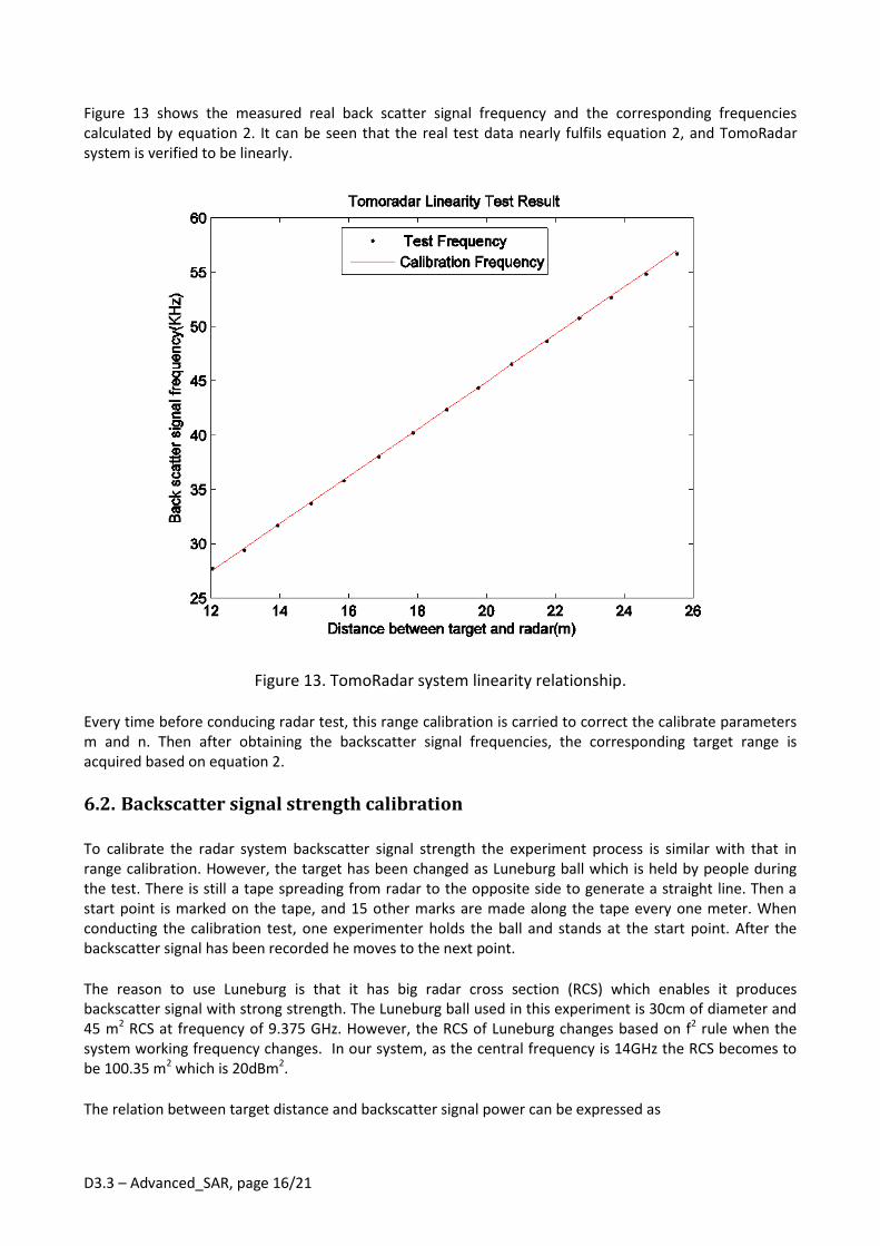
Figure 13 shows the measured real back scatter signal frequency and the corresponding frequencies calculated by equation 2. It can be seen that the real test data nearly fulfils equation 2, and TomoRadar system is verified to be linearly.

Figure 13. TomoRadar system linearity relationship.

Every time before conducing radar test, this range calibration is carried to correct the calibrate parameters m and n. Then after obtaining the backscatter signal frequencies, the corresponding target range is acquired based on equation 2.

6.2. Backscatter signal strength calibration

To calibrate the radar system backscatter signal strength the experiment process is similar with that in range calibration. However, the target has been changed as Luneburg ball which is held by people during the test. There is still a tape spreading from radar to the opposite side to generate a straight line. Then a start point is marked on the tape, and 15 other marks are made along the tape every one meter. When conducting the calibration test, one experimenter holds the ball and stands at the start point. After the backscatter signal has been recorded he moves to the next point.

The reason to use Luneburg is that it has big radar cross section (RCS) which enables it produces backscatter signal with strong strength. The Luneburg ball used in this experiment is 30cm of diameter and 45 m2 RCS at frequency of 9.375 GHz. However, the RCS of Luneburg changes based on f2 rule when the system working frequency changes. In our system, as the central frequency is 14GHz the RCS becomes to be 100.35 m2 which is 20dBm2.

The relation between target distance and backscatter signal power can be expressed as

D3.3 – Advanced_SAR, page 17/21

D4 =λ2G2PtGaσ

(4π)3∙1

Pr (3)

Where G is the antenna gain and Ga is the system amplifier gain; σ is the RCS of target; 𝜆 is wavelength of signal.

Backscatter signal strength calibration will be completed soon. With the experiment data, the relation between backscatter signal power and the target range will be researched. In other words, the relation presented by equation 3 will be verified and the power will be calibrated if necessary.

6.3. Range Resolution

6.3.1. One target resolution test

The system range resolution is calculated as R0= C/Beff, where C is light speed and B is system efficient bandwidth. In TomoRadar system the efficient bandwidth can be seen as the whole bandwidth which is 1 GHz. Thus the resolution of system is 15cm theoretically. To verify this resolution, the similar experiment in 6.1 is conducted. However, the target is designed to move 15cm every time instead of 1 meter. The length of the go-cart is a little bit less than one meter, thus the metal sheet was designed to be moved four times in total towards one direction. In the experiment, the go-cart was put in three different places; and the target was detected four times at different positions in each place. The go-cart is put in three different positions. One is near the radar, and one is far away from radar, while the last one locates in the middle of those two positions. More details and test results can be seen in Table 5.

Table 5. One target resolution test result.

Backscatter signal frequency (KHz)

Distance from radar to target (m)

Frequency difference with former recording(Hz)

Calibration backscatter signal frequency(KHz)

A 58.2 26.062 --------------------------------- 58.1

58.0 25.921 200 57.8

57.5 25.746 500 57.4

57.2 25.598 300 57.1

B

46.5 20.704 -------------------------------- 46.4

46.2 20.545 300 46.1

45.9 20.397 300 45.8

45.5 20.260 400 45.5

C

24.3 10.476 ------------------------------- 24.2

24.0 10.321 300 23.8

23.6 10.157 400 23.5

23.3 10.016 300 23.2

As Table 5 shows that no matter how far the target is away from radar, whenever the target moves 15 cm the frequency of backscatter signal changes corresponding frequency value. Thus the system resolution 15 cm is reached for one target.

D3.3 – Advanced_SAR, page 18/21

Through resolution test the calibration equation is verified at the same time. According to equation 2 the frequency changes should be 327 Hz when the target moves 15 cm. Table 5 shows the frequency difference is around 350Hz. With currently configuration of FFT conversion of oscilloscope card, the minimum resolution is 100Hz and the system cannot detect 100 Hz difference of the back scattered signal. Thus they nearly fulfilled equation 2. Moreover, the calibration backscatter signal frequencies have been calculated based on equation 2 in Table 5. Compare the calibration values and the practical values; the frequency difference is around 100Hz which is the minimum detectable value. Therefore the formula fulfils the system properties. However, there are some factors might affect the practical test results. Firstly, when conducted this test, one Low Noise Amplifier (LNA) is embedded in the radar system and the received backscattered signal has been amplified. More details about the effect of LNA will be researched later. Secondly, the backscatter signal frequency is read from the received signal diagram directly by experimenters which may cause deviations. Thirdly, it is difficult to exactly assure that where the signal emits from radar, from the mixer where LO signal mixed with DDS IF signal or the feed centre of parabolic antenna. Therefore, we have to estimate the start point based on principle understanding of physical nature. Thus there must be some deviation between the exact distance and the measured distance. All these factors may cause the difference between practical signal frequency and calibrated values.

6.3.2. Two targets resolution test

Theoretically when there are two targets, the radar system should detect them separately when the distance between two targets is at least 15 cm. The similar experiment with 6.3.1 has been done to verify this theoretically resolution value. Besides the former metal sheet one more metal sheet with smaller size is employed. Both of two metal sheets are put on the wood go-cart, while the smaller one stands before the bigger one to guarantee that both targets reflect signal. Figure 14 shows how the targets are arranged.

Figure 14 Two target resolution test

When conducting the experiment, the wood go-cart is put in three different positons and the distance between two targets is changed. Table 6 shows the results.

D3.3 – Advanced_SAR, page 19/21

According to Table 6 , No matter how far the targets are away from radar, when the distance between two targets is 50 cm they can be recognized easily. However, when the distance between two targets decreases to be 30 cm whether they can be recognized depends on their position. If there is no big interference around target and the targets are a little far from radar (still in the detect range), then they can be recognized. However, when there is big interference, it’s difficult to recognize two targets respectively. Thus for two targets the resolution cannot reach 15cm. From single target resolution test, it is sure that the backscatter signal strength is strong enough. However, when there are two targets, as each backscatter signal in frequency domain is wide, then the two backscatter signal is merged in frequency domain.

Table 6. Two target resolution test.

Backscatter signal frequency-front(KHz)

Backscatter signal frequency-back(KHz)

Distance between front sheet and radar(m)

Distance between two metal sheet (cm)

A 23.4 24.3 10.04 50

23.6 Two peaks merges 10.235 30

B 44 45.1 19.578 50

44.4 45.1 19.777 30

44.3~45.4 , two peaks merges together, only a wide pulse

19.879 20

44.6~45.3, signal is not stable, sometimes merges and sometimes separate

19.928 15

C 60.3 61.4 27.044 50

Two peaks merges together, caused a little by the trees around(big interference)

27.243 30

In addition, environment noise has a bad effect on the test. Even though we have utilized the wood cart as a platform to carry the metal sheet target, the wood structure of the cart frame still reflect the transmitted RF signal which might expend the width of target in frequency domain which results in that two targets could not be recognized after FFT. Similar effects have been produced by the environment. Both the trees around target and floor noise reflect signal which is some kind of noise to radar.

6.4. Calibration Results

Until this stage, the range calibration of TomoRadar has been completed as shown before. The system has been proved to be linear which means the target range can be acquired simply from our linear equation. With this calibration result the range calculation process is simply but result is precise. However, how it fulfils the long range situation will be researched later with the data obtained from the helicopter test. Power calibration is planned to be completed soon as well.

Furthermore, the calibration process figures out the least distance between two targets required to be recognized by TomoRadar. However, the system resolution is verified as well. With these conclusions, the scanned results of TomoRadar can be analysed in more details. What’s more, these factors are meaningful when considering TomoRadar applications with different system sensitivity requirement.

D3.3 – Advanced_SAR, page 20/21

7. Conclusion

Several preliminary conclusions could be drawn based on the field test, car-borne test and helicopter tests. 1. The functionality of the Tomoradar has been successfully fulfilled; 2. Tomoradar can discriminate the two targets when the distance between them are more than 30

cm; 3. the range resolution of Tomoradar is 15 cm which is same as that in project plan; 4. The effective maximum range distance is at least 250 meters which is higher than the designed

parameter, we assume the maximum range of current configuration is about 400 meters with minor modification on IF parts, which means it might be also use for gasoline-drive fix wing UAV. It implies that the application scope for Tomoradar might be more extendable than former anticipation;

5. The current Tomoradar is light weight, and the size of two antennas (including the separation) is less than 70 cm; which implies it can be integrated in a Mini-UAV platform.

8. Full polarization Tomoradar

Extension to the previous one channel version Tomoradar into 2 channels (HH and HV), and finally into full polarimetry (HH, VV, HV and VH) system as Figure 15 presents has been done. The field test in EVO site has already been carried out with leaf on (2015.10 and 2015.9) and leaf off (2015.12) situations. Some electronics models for IF part is redesigned and upgraded based on the first airborne test. The noise floor of the real time FFT has been decreased to -80-90 dB, which is 15-20 dB lower than the previously version. The precise report about the field test the data quality will be reported in next report period.

Figure 15. The diagram of the full polarimetric system.

D3.3 – Advanced_SAR, page 21/21

9. Future activities

We will continue the FGI-Tomoradar campaign by comparing results against other RS data from the Evo area. From the scientific point of view, other frequency bands should be investigated for different research purposes. For example, 9.4 GHz might be a candidate frequency bank to select to compare the previous results collected by HUTSCAT.