ADVANCED CONCEPTS IN POLARIMETRIC SAR IMAGE ANALYSIS

A TUTORIAL REVIEW

Eric POTTIER(1), Jong-Sen LEE(2), Laurent FERRO-FAMIL(1)

(1): I.E.T.R – UMR CNRS 6164, University of Rennes1 Image and Remote Sensing Department, SAPHIR Team Campus de Beaulieu, Bat 11D, 263 Av Gal Leclerc F-35042 Rennes cedex, France e-mail : eric.pottier@univ-rennes1.fr,

laurent.ferro-famil@univ-rennes1.fr (2): Naval Research Laboratory

Remote Sensing Division Washington, DC 20375-5351 USA e-mail : lee@ccf.nrl.navy.mil

ABSTRACT

There is currently widespread interest in the development of radar sensors for the detection of surface and buried targets and the remote sensing of land, sea and ice surfaces. An important feature of electromagnetic radiation is its state of polarisation and a wide range of classification algorithms and inversion techniques have recently been developed based on the transformation of polarisation state by scattering objects. There are three primary ways in which multi-parameter radar measurements can be made: multi-frequency, single or multi-baseline interferometry and multi-polarization. While several airborne systems can now provide diversity over all three of these, it is the combination of polarimetry with interferometry at a single wavelength that forms the central focus of future challenges in developing new and original data processing. The main reason for this is the imminent launch of a series of advanced satellite radar systems such as PALSAR, an L-band SAR sensor on board the NASDA ALOS satellite and Radarsat II, a C-band polarimetric sensor. These are typical of a new generation of radars with the potential for providing data from various combinations of polarimetry and interferometry.

This paper seeks to review recent progress in polarimetric and interferometric SAR data processing, covering advances and addressing the important topic of classification of polarimetric SAR data.

1 INTRODUCTION

SAR remote sensing allows all weather, global scale imaging and estimation of important bio and geophysical parameters about the Earth's surface. This is achieved by sensing scattered electromagnetic fields reflected from the Earth surface when emitted by an electromagnetic energy source situated on an aircraft, spacecraft or satellite outside of the Earth's atmosphere. The development of multi-parameter SAR techniques such as Polarimetric SAR (POLSAR) and Interferometric SAR (InSAR) is advancing rapidly, and these novel radar technologies are constantly extending the range of applications of radar in remote sensing.

Radar Polarimetry (Polar: polarization Metry: measure) is the science of acquiring, processing and analysing the polarization state of an electromagnetic field. The polarization information contained in the waves backscattered from a given medium is highly related to its geometrical structure and orientation as well as to its geophysical properties such as humidity, roughness and conductivity of soils, . . . . .

Radar Polarimetry deals with the full vector nature of polarized electromagnetic waves, and when the wave passes through a medium of changing index of refraction, or when it strikes an object or a scattering surface and it is reflected; then, characteristic information about the reflectivity, shape and orientation of the reflecting body can be obtained by implementing polarization processing [Boerner 1998]. Whereas with radar polarimetry the textural fine-structure, target-orientation and shape, symmetries and material constituents of the Earth surface can be recovered with considerable improvements above that of standard “amplitude-only radar”; with radar interferometry the spatial structure can be explored. More recently, Radar Interferometry has matured as an important sensing technology for topographic mapping and land classification [Bamler 1998]. By combining interferograms in different polarisation states it has been shown that important structural information relating to vegetation height and density can be obtained [Cloude 1998]. Combining polarimetric and interferometric SAR techniques (POL-IN-SAR) it is today possible to recover such co-registered textural plus spatial properties simultaneously. This has important consequences for the design of future space and airborne sensors for carbon sequestration and climate change studies.

Thanks to the new polarimetric radar sensors (ENVISAT ASAR and the future RADARSAT-2 and ALOS-PALSAR, TerraSAR X & L), it is now shown that the accelerated advancement of POLSAR techniques is of direct relevance and of priority to local-to-global environmental ground-truth measurement and validation, stress assessment, and stress-change monitoring of the terrestrial and planetary covers. POLSAR remote sensing offers an efficient and reliable means of collecting the information required in order to extract the biophysical and geophysical parameters about the Earth's surface and have found successful application in crop monitoring and damage assessment, in forestry clear cut mapping, deforestation and burn mapping, in land surface structure (geology) land cover (biomass) and land use, in hydrology (soil moisture, flood delineation), in sea ice monitoring, in oceans and coastal monitoring (oil spill detection) etc …

Today, it can be said that there is more and more a rapidly increasing interest in the use of radar polarimetry and interferometry for radar remote sensing; and wave polarization is today of fundamental importance in the information retrieval problem of microwave imaging and inverse scattering.

2 POLARIMETRIC SAR DATA ANALYSIS 2.1 TARGET VECTOR FOR BACKSCATTER PROBLEMS.

An important development in our understanding of how to best extract physical information from the classical 2x2 coherent backscattering matrix [S] has been achieved through the construction of system vectors [Cloude 1996][Cloude 1997]. We represent this vectorization of a matrix by the vector V(.) built as follows :

[ ] [ ]( ) [ ][ ](SS SS S k V S Trace SXX XY

XY YY=

⇒ = =

12

ψ ) (1)

where Trace([A]) is the sum of the diagonal elements of matrix [A] and [ψ] is a set of 2x2 complex basis matrices which are constructed as an orthonormal set under an hermitian inner product [Cloude 1986][ Cloude 1996]. There exist in the literature different basis sets, but the special set used to generate 3x3 coherency matrix [T] is based on linear combinations arising from the Pauli matrices, and is given by:

[ ]ψ =

−

21 00 1 2

1 00 1 2

0 11 0, , (2)

where the factor 2 arises from the requirement to keep the norm of the target vector k invariant, equal to the Frobenius norm (Span) of the backscattering matrix [S], namely the total power scattered by the target. The target vector k has the explicit form shown in (3).

[k S S S S SXX YY XX YY XY

T= + −

12

2 ] (3)

With such a vectorization we can then generate a coherency matrix from the outer

product of the target vector k with its conjugate transpose. For the monostatic case, the 3x3 hermitian coherency matrix [T] has the following parameterisation [Cloude 1996]:

[ ]T k kA C jD H jG

C jD B B E jFH jG E jF B B

T= ⋅ =− +

+ + +− − −

*

2 0

0

0

(4)

where A0, B0, B, C, D, E, F, G and H are the « Huynen parameters » identified as phenomenological target parameters interrelated in such a way as to reflect directly the physical source of correlation effects in the target. These nine parameters are useful for general target analysis without reference to any model, and each of them contains real physical target information [Huynen 1970][Pottier 1992].

The parameters A0, B0+B and B0 - B, called the « target generators », are connected respectively with the symmetry, irregularity / double bounce and non-symmetry physical properties in the case of a pure target (strong scatterer) [Huynen 1970][Pottier 1992], or related to surface scattering, double-bounce scattering and volume scattering in the case of a distributed target (natural media).

It is thus possible to use these « target generators » to create a color coding for PolSAR images, by assigning respectively the color red for VVHH0 SSBB −=+ , green for

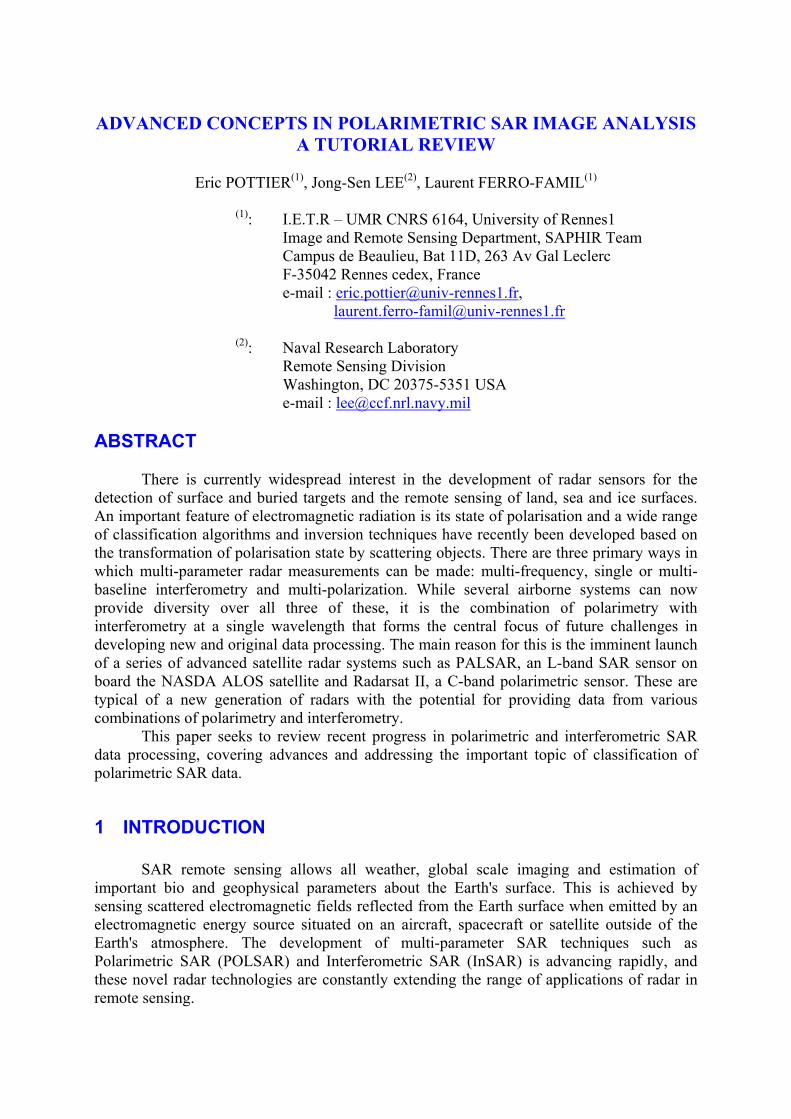
, and blue for |S|BB HV0 =− VVHH0 SSA2 += . For illustration, the well known NASA/JPL AIRSAR L-Band full polarimetric SAR image of San Francisco Bay (1988) and the DLR E-SAR L-Band full polarimetric SAR image of Oberpfaffenhofen (Germany) are shown respectively on Figs. 1 and 2.

Fig. 1 : Pauli color coded image of the San Francisco Bay.

Fig. 2: Optical image and Pauli color coded image over Oberpfaffenhofen (Germany)

In these two displays, the polarimetric channel combinations play an important role in separating ocean surface or agricultural areas (surface scattering), forests, vegetation and trees (volume scattering), and urban areas (double bounce scattering) which composed the different scenes.

Called the “Pauli coding representation”, this adopted color coding has become today the standard for PolSAR image display. 2.2 POLARIMETRIC SAR DATA STATISTICS A polarimetric radar measures the complete scattering matrix [S] of a medium at a given incidence angle and for a given frequency. This scattering matrix with complex elements can be expressed in a vector form, following :

[X S S SHH HV VV

T= 2 ] (5)

where the factor 2 arises from the requirement to keep the norm of the target vector X an invariant, equal to the Frobenius norm (Span) of the backscattering matrix [S], namely the total power scattered by the target.

When the radar illuminates an area of a random surface of many elementary scatterers, the one-look scattering vector X can be modeled as having a multivariate complex Gaussian probability density function [Lee 1999b], with :

( ) [ ][ ]P X e

CX C XT

= − −1

3

1

π

*

(6)

where [C]=E(X XT*)is the hermitian covariance matrix of the scattering vector X.

As the target vector k is constructed from a linear combination of the elements of the scattering vector X, following :

kS SS S

S

SS

S

HH VV

HH VV

HV

HH

HV

VV

=+−

= −

12

2

12

1 0 11 0 10 2 0

2 (7)

the elements of the target vector k are considered as having the same complex Gaussian distribution than the elements of the scattering vector X.

POLSAR data are frequently multi-look processed for speckle reduction, or data compression. The relative polarimetric information is thus contained in the expected value of the coherency matrix <[T] > representing the spatial-averaged distributed target given by :

[ ] [TN

k kN

Ti iT

i

N

ii

N

= ⋅ == =∑1 1

1 1

* ]∑ (8)

where [Ti] is a single-look coherency matrix of the ith pixel.

It has been shown in [Lee 1999b] that the averaged coherency matrix <[T]> has a complex Wishart distribution. The probability density function is given by :

[ ] [ ]( ) [ ] [ ] [ ]( )

( ) ( ) [ ]P T T

L T e

L L p Tm

Lp L p L Tr T T

m

L

m

p p/...

( )=− +

− −−

−

1

12 1π Γ Γ

(9)

where [Tm] is global coherency matrix with [Tm] = E(k kT*), L is the number of look and p the dimension of the target vector k, with p=3 for the reciprocal case (SHV=SVH) and p=4 for the non-reciprocal case.

The distribution functions for dual polarization (HH, VH), (HV, VV) or (HH, VV) can be derived from this complex Wishart distribution. For example, if only complex HH and VV are available, p=2, and for single polarization, p=1, which reduces (9) to the Chi-square distribution with 2L degree of freedom.

For the dual polarization case without phase difference information (|HH|, |VV|), the probability density function has been derived [Lee 1994a]. Letting >=< 2

HH1 SR and

>=< 2VV2 SR , we have:

−⋅

−

−+

−

= −−+

−+

2c

c

2211

211n1n

c2

c2/)1n(

2211

2c

2221112)1n(

211n

21 ||1||

CCRR

n2I||)||1)(n()CC(

||1)C/RC/R(n

exp)RR(n)R,R(p

ρρ

ρρΓρ

(10) where is the modified Bessel function of the nth order,( )nI [ ]111 REC = and C . [ ]222 RE=

3 POLARIMETRIC TARGET DECOMPOSITION THEOREMS

There is currently a great deal of interest in the use of polarimetry for radar remote sensing. In this context, an important objective is to extract physical information from the observed scattering of microwaves by surface and volume structures. The most important observable measured by such radar systems is the 3x3 coherency matrix [T]. This matrix accounts for local variations in the scattering matrix and is the lowest order operator suitable to extract polarimetric parameters for distributed scatterers in the presence of additive (system) and/or multiplicative (speckle) noise.

Many targets of interest in radar remote sensing require a multivariate statistical description due to the combination of coherent speckle noise and random vector scattering effects from surface and volume. For such targets, it is of interest to generate the concept of an average or dominant scattering mechanism for the purposes of classification or inversion of scattering data. This averaging process leads to the concept of the « distributed target » which has its own structure, in opposition to the stationary target or « pure single target » [Huynen 1970][Pottier 1992].

Target Decomposition theorems are aimed at providing such an interpretation based on sensible physical constraints such as the average target being invariant to changes in wave polarization basis.

Target Decomposition theorems were first formalized by J.R. Huynen but have their roots in the work of Chandrasekhar on light scattering by small anisotropic particles. Since this original work, there have been many other proposed decompositions. We classify four main types of theorem:

1. Those employing coherent decomposition of the scattering matrix (Krogager, Cameron).

2. Those based on the dichotomy of the Kennaugh matrix (Huynen, Barnes). 3. Those based on a “model-based” decomposition of the covariance or the

coherency matrix (Freeman and Durden, Dong). 4. Those using an eigenvector / eigenvalues analysis of the covariance or

coherency matrix (Cloude, VanZyl, Cloude and Pottier).

A complete description of all these different Polarimetric Target Decomposition can be found in [Cloude 1996], and we focus here on the H / A / α decomposition theorem which will be used further in the polarimetric classifications. 3.1 THE H / A / α POLARIMETRIC DECOMPOSITION THEOREM

In 1997, S.R. Cloude and E. Pottier proposed a method for extracting average parameters from experimental data using a smoothing algorithm based on second order

statistics [Cloude 1997]. This method does not rely on the assumption of a particular underlying statistical distribution and so is free of the physical constraints imposed by such multivariate models. An eigenvector analysis of the 3x3 coherency matrix [T] is used since it provides a basis invariant description of the scatterer and also provides a decomposition into types of scattering process (the eigenvectors) and their relative magnitudes (the eigenvalues). This original method, based on an eigenvalue analysis of the coherency matrix, employs a 3-level Bernoulli statistical model to generate estimates of the average target scattering matrix parameters. This alternative statistical model sets out with the assumption that there is always a dominant 'average' scattering mechanism in each cell and then undertakes the task of finding the parameters of this average component [Cloude 1997].

3.1.1 EIGENVECTOR-BASED DECOMPOSITION. The instantaneous (single pixel) target return from a spatially extended target can be characterized either by its complex scattering matrix [S] which relates to received spatial-voltage, or by its 3x3 coherency matrix [T] which relates to spatial-power. In the case of spatial-averaging, it is customary to consider the expected value of the coherency matrix <[T]> as representing the averaged distributed target, as :

[ ] [ ]TN

k kN

Ti iT

i

N

ii

N

= ⋅ == =∑1 1

1 1

* ∑ (11)

From this estimate, the eigenvectors and eigenvalues of the 3x3 hermitian coherency matrix <[T]> can be calculated to generate a diagonal form of the coherency matrix which can be physically interpreted as statistical independence between a set of target vectors [Cloude 1992][ Cloude 1996]. The coherency matrix <[T]> can be written in the form of:

[ ] [ ][ ][ ] 133 UUT −= Σ (12)

where [ ]Σ is a 3x3 diagonal matrix with nonnegative real elements, and [ ] [ ]3213 uuuU = is a 3x3 unitary matrix of the SU(3) group, where u1, u2, and u3 are the three unit orthogonal eigenvectors.

By finding the eigenvectors of the 3x3 hermitian coherency matrix <[T]>, such a set of 3 uncorrelated targets can be obtained and hence a simple statistical model can be constructed, consisting of the expansion of <[T]> into the sum of 3 independent targets, each of which, represented by a single scattering matrix. This decomposition can be written following:

[ ] [ ] ∑∑=

=

=

=

⋅==3i

1i

T*iii

3i

1iii uuTT λλ (13)

where the real numbers λi are the eigenvalues of <[T]> and represent statistical weights for the three normalized component targets [Ti] [Cloude 1992]. If only one eigenvalue is nonzero then the coherency matrix <[T]> corresponds to a pure target and can be related to a single scattering matrix. On the other hand, if all eigenvalues are equal, the coherency matrix <[T]> is composed of three orthogonal scattering

mechanisms with equal amplitudes, the target is said random and there is no correlated polarized structure at all.

Between these two extrema, there exists the case of partial targets and where the coherency matrix <[T]> has non-zero and non-equal eigenvalues. The analysis of its polarimetric properties requires a study of the eigenvalues distribution as well as a characterization of each scattering mechanism of the expansion.

To introduce the degree of statistical disorder of each target, the entropy (H) is defined

in the Von Neumann sense from the logarithmic sum of eigenvalues of <[T]> [Cloude 1996][Cloude 1997], as:

(∑=

=

−=3i

1ii3i PlogPH ) (14)

where Pi are the probabilities obtained from the eigenvalues λi of <[T]> with:

Pii

jj

j=

=

=

∑

λ

λ1

3 (15)

If the entropy H is low then the system may be considered as weakly depolarizing and the dominant target scattering matrix component can be extracted as the eigenvector corresponding to the largest eigenvalue and ignore the other eigenvector components. If the entropy H is high then the target is depolarizing and we can no longer consider it as having a single equivalent scattering matrix. The full eigenvalue spectrum must be considered. Further, as the entropy H increases, the number of distinguishable classes identifiable from polarimetric observations is reduced. In the limit case, when H=1, the polarization information becomes zero and the target scattering is truly a random noise process . While the entropy is a useful scalar descriptor of the randomness of the scattering problem, it is not a unique function of the eigenvalue ratios. Hence, another eigenvalue parameter defined as the anisotropy A can be introduced, with :

A =−+

λ λλ λ

2

2 3

3 (16)

When A=0 the second and third eigenvalues are equal. The anisotropy may reach such a value for a dominant scattering mechanism, where the second and third eigenvalues are close to zero, or for the case of a random scattering type where the three eigenvalues are equal. The condition for <[T]> to have such an equivalent scattering matrix [S] is for both the target entropy H and the anisotropy A to be equal to zero, which corresponds to a single nonzero eigenvalue (λ1) [Cloude 1992][Cloude 1996]. In this case the coherency matrix <[T]> has rank r=1, and can be expressed as the outer product of a single target vector k1 with:

[ ]T k k u uT= ⋅ = ⋅1 1 1 1 1

* λ T* (17)

where is equal to the Frobenius norm (Span) of the corresponding scattering matrix, and where the corresponding unit target vector is expressed as follows :

(λ1 02= +A B )0

ue j

A

AC jDH jG

e j A

B B e j D C

B B e j G H1

0 1

0

1

0

0

0

2

2 2

= +−

= + +

− −

φ

λ

φ

λarctan( / )

arctan( / ) (18)

It is interesting to note that the modulus of the three components of the unit target vector are directly function of the three « Huynen target generators ». Without using ground truth measurements, this polarimetric parameterisation of the unit target vector u involves the fit of a combination of three simple scattering mechanisms : surface scattering, dihedral scattering and volume scattering, which are characterized from the three components (target generators) of the unit target vector such as: Surface scattering: A0 >> B0 +B , B0 - B Dihedral scattering: B0 + B >> A0 , B0 - B Volume scattering: B0 - B >> A0 , B0+B

3.1.2 PROBABILISTIC MODEL FOR RANDOM MEDIA SCATTERING. In previous publications [Cloude 1995] [Cloude 1996] [Cloude 1997], a parameterisation of the eigenvectors of the 3x3 coherency matrix [T] has been introduced for the case of scattering medium which does not have azimuthal symmetry [Nghiem 1992], and which takes the form shown in (19).

u e j e j T

=

cos sin cos sin sinα α β δ α β γ (19)

It follows a revised parameterisation of the coherency matrix [Cloude 1997], as :

[ ] [ ] [ ]T U U3=

λλ

λ

1

2

3

0 00 00 0

*T

3 (20)

[ ] ( ) ( )( ) ( )

U e je j e j

e j e j e j

e j e j e j3

1

2 3

11

2 22 2

3 33 3

1 11

2 22 2

3 33 3

1=+ +

+ +

φα α φ α φ

α β δ α β δ φ α β δ φ

α β γ α β γ φ α β γ φ

cos cos cos

sin cos sin cos sin cos

1 2 3

sin sin sin sin sin sin

(21)

The parameterisation of a 3x3 unitary matrix [U3] in terms of column vectors with different parameters α1 β1 etc... is made so as to enable a probabilistic interpretation of the scattering process. In general, the columns of the 3x3 unitary matrix are not only unitary but mutually orthogonal. This means that in practice α1 α2 and α3 are not independent.

In this case a statistical model of the scatterer is considered as a 3 symbol Bernoulli process i.e. the target is modeled as the sum of three [S] matrices, represented by the columns of [U3] in (21), occuring with probabilities Pi ,given from (15) by the normalized eigenvalues so that P1 + P2 + P3 = 1 [Cloude 1997]. In this way for example, the parameter α follows a random sequence:

α α α α α α α α α α= 1 2 3 2 1 2 3 1 1 K (22) and the best estimate of this parameter is given by the mean of this sequence, easily evaluated as [Cloude 1997] :

α α α α= + +P P P1 1 2 2 3 3 (23) In this way, the mean parameters of the dominant scattering mechanism are extracted from the 3x3 coherency matrix as a mean target vector u0, such that:

u e j e j

ej

0 =

φα

α β δ

α βγ

cos

sin cos

sin sin

(24)

where the parameters α β δ and γ are defined in (19), and where φ is physically equivalent to an absolute phase.

3.1.3 THE ROLL INVARIANCE PROPERTY. One of the most important property in Radar Polarimetry concerns the roll invariance. The effect of rotation around the radar line of sight [Cloude 1996] can be generated as:

( )[ ] [ ] [ ] [ ]T U T URθ =−

3

1R3

]

2θ

(25) where [ is the unitary similarity rotation matrix, given by: U R

3

[ ]U R3

1 0 00 2 20 2

=−

cos sinsin cos

θθ θ

(26)

According to the eigenvector-based decomposition approach, the coherency matrix can be written in the form of:

( )[ ] [ ][ ][ ][ ] [ ] [ ][ ][ ]T U U U3 3 3 3θ = = ′ ′−

U UR T R T

3 3

1Σ

*UΣ

* (27)

[ ] [ ][ ] ( ) ( )( ) ( )

′ = =

′ ′

′ ′ ′′ + ′

′′ + ′

′ ′ ′′ + ′

′′ + ′

U U e je j e j

e j e j e j

e j e j e j

R3 3

1

2 3

11

2 22 2

3 33 3

1 11

2 22 2

3 33 3

1U

cos cos cos

sin cos sin cos sin cos3

1 2 3

φα α φ α φ

α β δ α β δ φ α β δ φ

α β γ α β γ φ α β γ φsin sin sin sin sin sin

(28)

where is the same 3x3 diagonal matrix with nonnegative real elements. [ ]Σ

[ ] [′ =U v v v3 1 2 3 ] is the new 3x3 unitary matrix of the SU(3) group, where v1, v2, and v3 are the new three unit orthogonal eigenvectors. Following the parameterisation of the 3x3 unitary matrix [U’3], it can be seen that the three parameters α1 α2 and α3 remain invariant, as the three eigenvalues (λ1 λ2 λ3). It follows that the mean parameter α, and the two important scalar functions of the eigenvalues, the entropy H and the anisotropy A, are three roll-invariant parameters. Among the mean parameters (α, β, δ and γ) of the dominant scattering mechanism which can be extracted from the 3x3 coherency matrix, it is now clear from the above analysis, that for random media problems, the main parameter for identifying the dominant scattering mechanism is α. The three others parameters (β, δ and γ) can be used to define the target polarisation orientation angle [Pottier 1998][Pottier 1999][Schuler 1999]. In previous publication [Cloude 1997], it has been shown that the useful range of the parameter α corresponds to a continuous change from surface scattering in the geometrical optics limit (α=0°) through surface scattering under physical optics to the Bragg surface model, encompassing dipole scattering or single scattering by a cloud of anisotropic particles (α=45°), moving into double bounce scattering mechanisms between two dielectric surfaces and finally reaching dihedral scatter from metallic surfaces (α=90°). The α parameter estimate is related directly to underlying average physical scattering mechanism, and hence may be used to associate observables with physical properties of the medium [Cloude 1997]. Fig. 3 shows these three roll-invariant parameters : H, A and α.

0 0.5 1 Entropy H

0 0.5 1 Anisotropy A

0° 45° 90°

α parameter Fig. 3 : Roll-invariant parameters : H, A and α

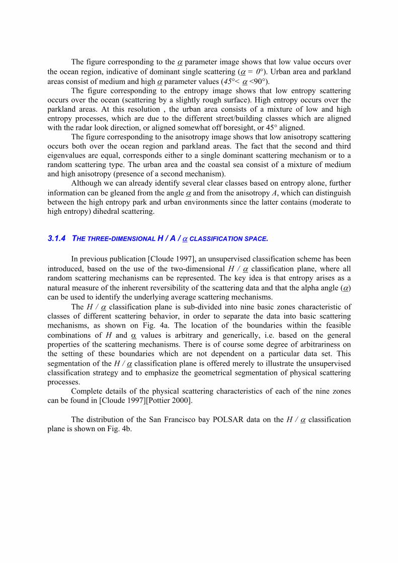
The figure corresponding to the α parameter image shows that low value occurs over the ocean region, indicative of dominant single scattering (α = 0°). Urban area and parkland areas consist of medium and high α parameter values (45°< α <90°). The figure corresponding to the entropy image shows that low entropy scattering occurs over the ocean (scattering by a slightly rough surface). High entropy occurs over the parkland areas. At this resolution , the urban area consists of a mixture of low and high entropy processes, which are due to the different street/building classes which are aligned with the radar look direction, or aligned somewhat off boresight, or 45° aligned. The figure corresponding to the anisotropy image shows that low anisotropy scattering occurs both over the ocean region and parkland areas. The fact that the second and third eigenvalues are equal, corresponds either to a single dominant scattering mechanism or to a random scattering type. The urban area and the coastal sea consist of a mixture of medium and high anisotropy (presence of a second mechanism). Although we can already identify several clear classes based on entropy alone, further information can be gleaned from the angle α and from the anisotropy A, which can distinguish between the high entropy park and urban environments since the latter contains (moderate to high entropy) dihedral scattering.

3.1.4 THE THREE-DIMENSIONAL H / A / α CLASSIFICATION SPACE. In previous publication [Cloude 1997], an unsupervised classification scheme has been introduced, based on the use of the two-dimensional H / α classification plane, where all random scattering mechanisms can be represented. The key idea is that entropy arises as a natural measure of the inherent reversibility of the scattering data and that the alpha angle (α) can be used to identify the underlying average scattering mechanisms. The H / α classification plane is sub-divided into nine basic zones characteristic of classes of different scattering behavior, in order to separate the data into basic scattering mechanisms, as shown on Fig. 4a. The location of the boundaries within the feasible combinations of H and α values is arbitrary and generically, i.e. based on the general properties of the scattering mechanisms. There is of course some degree of arbitrariness on the setting of these boundaries which are not dependent on a particular data set. This segmentation of the H / α classification plane is offered merely to illustrate the unsupervised classification strategy and to emphasize the geometrical segmentation of physical scattering processes. Complete details of the physical scattering characteristics of each of the nine zones can be found in [Cloude 1997][Pottier 2000]. The distribution of the San Francisco bay POLSAR data on the H / α classification plane is shown on Fig. 4b.

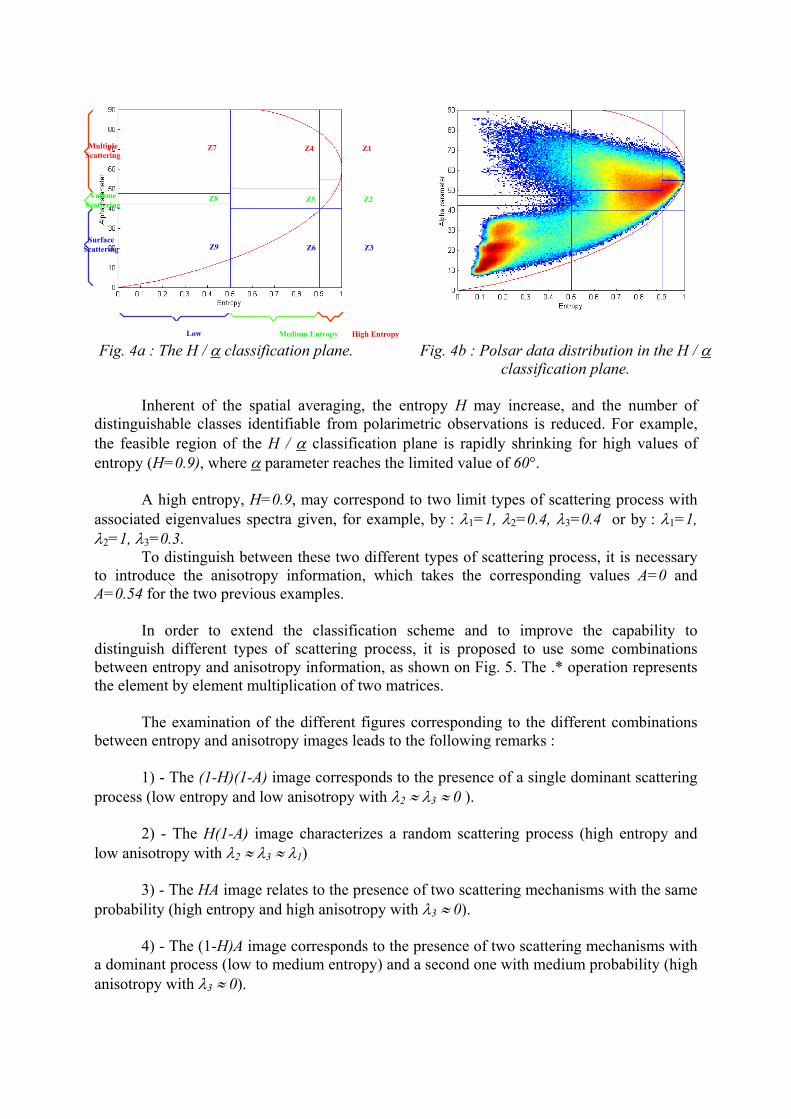
Fig. 4a : The H / α classification plane. Fig. 4b : Polsar data distribution in the H / α classification plane.

Multiple Scattering

Z7 Z4 Z1

Volume Scattering

Z8 Z5 Z2

Surface Scattering Z9 Z6 Z3

Low Medium Entropy High Entropy

Inherent of the spatial averaging, the entropy H may increase, and the number of distinguishable classes identifiable from polarimetric observations is reduced. For example, the feasible region of the H / α classification plane is rapidly shrinking for high values of entropy (H=0.9), where α parameter reaches the limited value of 60°. A high entropy, H=0.9, may correspond to two limit types of scattering process with associated eigenvalues spectra given, for example, by : λ1=1, λ2=0.4, λ3=0.4 or by : λ1=1, λ2=1, λ3=0.3. To distinguish between these two different types of scattering process, it is necessary to introduce the anisotropy information, which takes the corresponding values A=0 and A=0.54 for the two previous examples. In order to extend the classification scheme and to improve the capability to distinguish different types of scattering process, it is proposed to use some combinations between entropy and anisotropy information, as shown on Fig. 5. The .* operation represents the element by element multiplication of two matrices. The examination of the different figures corresponding to the different combinations between entropy and anisotropy images leads to the following remarks : 1) - The (1-H)(1-A) image corresponds to the presence of a single dominant scattering process (low entropy and low anisotropy with λ2 ≈ λ3 ≈ 0 ). 2) - The H(1-A) image characterizes a random scattering process (high entropy and low anisotropy with λ2 ≈ λ3 ≈ λ1) 3) - The HA image relates to the presence of two scattering mechanisms with the same probability (high entropy and high anisotropy with λ3 ≈ 0). 4) - The (1-H)A image corresponds to the presence of two scattering mechanisms with a dominant process (low to medium entropy) and a second one with medium probability (high anisotropy with λ3 ≈ 0).

Fig. 5 : Combinations between entropy and anisotropy images.

(1-H)(1-A)

.*

(1-H)

A

(1-A)

(1-H)A

HA

H(1-A)

H

0 0.5 1(For all images)

These remarks are confirmed by the analysis of the distribution of the San-Francisco bay POLSAR data in the extended and complemented three-dimensional H / A / α classification space, as shown on Fig. 6 This representation shows that it is possible to discriminate new classes using the anisotropy value.

For example, it is now possible to notice that there exists in the « Low Entropy Surface Scattering » area (Z9) a second class associated with a high anisotropy value and which corresponds to the presence of a second physical mechanism which is not negligible. Identical remarks can be made concerning the « Medium Entropy Vegetation Scattering » area (Z5) and the « Medium Entropy Multiple Scattering » area (Z4). Due to the spread of the POLSAR data along the anisotropy axis, it is now possible to improve the capability to distinguish different types of scattering process which have quite the same high entropy value: - High entropy and low anisotropy correspond to random scattering. - High entropy and high anisotropy correspond to the presence of two scattering mechanisms with the same probability.

Fig. 6 : Distribution of the San-Francisco bay POLSAR data in the

H / A / α classification space

From the analysis of the different images shown on Fig. 5 and from the distribution of the San-Francisco bay POLSAR data in the H / A / α classification space shown on Fig. 6., we can conclude that the anisotropy has to be considered now as a key parameter in the polarimetric analysis and/or inversion of POLSAR data. The information contained in these three roll-invariant parameters extracted from the local estimate of the 3x3 hermitian coherency matrix <[T]>, corresponds to the type of scattering process which occurs within the pixel to be classified (combination of entropy H and anisotropy A) and to the corresponding physical scattering mechanism (α parameter).

4 SUPERVISED POLARIMETRIC CLASSIFICATION

The selection of radar frequency and polarization are two of the most important parameters in synthetic aperture radar (SAR) mission design. Of course, a multi-frequency fully polarimetric SAR system is highly desirable, but the limitations of payload, data rate, budget, required resolution, area of coverage, etc. frequently prevent multi-frequency fully polarimetric SAR from becoming a reality, especially in a space-borne system. For a particular application, it is desirable to optimally select the frequency and combination of linear polarization channels, if a fully polarimetric SAR system is not possible, and to find out the expected loss in classification and geophysical parameter accuracy.

In this section, we quantitatively compare crop and tree classification accuracies between fully polarimetric SAR and partial polarimetric SAR for P-, L- and C-band frequencies. Using polarimetric P-, L- and C-band data from NASA/JPL AIRSAR [VanZyl 1990], we quantitatively compare the correct classification rates of crops and tree ages for all combinations of polarizations. Additionally, to understand the importance of phase differences between polarizations, we compare the correct classification rates using the complex HH and VV versus using the two intensity images without their phase difference.

The methodology introduced should have an impact on selecting the combinations of polarizations and frequency of a SAR for use in various applications. For example, the future C-band ENVISAT ASAR [Desnos 1999] system will have dual-polarization and single polarization/single polarization modes, and the C-band RADARSAT II [Meisl 2000] and L-band ALOS-PALSAR [Wakabayashi 1998] will also have the same modes for wider swatch selection, in additional to a fully polarimetric SAR mode.

To quantitatively evaluate the classification capability for various combinations of polarization, a procedure must be carefully established:

1. Optimal supervised classification algorithms developed from the same concept should be used for all combinations of polarizations

2. Training sets have to be carefully selected from the available ground truth map 3. The classification reference map to be used for the classification evaluation

must be reasonable and consistent with the ground truth map and polarimetric SAR data.

Comparison of classification accuracies between fully polarimetric, dual polarization

and single polarization SAR data have been evaluated for P-band, L-band and C-band using two JPL AIRSAR data sets: Flevoland for crops and Les Landes for tree ages. The availability of these multi-frequency polarimetric SAR data enables us to quantitatively compare classification capabilities of all combinations of polarizations for three frequencies. Furthermore, we have ground truth maps for both scenes that facilitate the selections of training sets and reference maps. 4.1 THE SUPERVISED WISHART CLASSIFIER The presented supervised algorithm, is a maximum likelihood classifier based on the complex Wishart distribution for the polarimetric coherency matrix, given by:

[ ] [ ]( ) [ ] [ ] [ ]( )

( ) ( ) [ ]P T T

L T e

L L p Tm

Lp L p L Tr T T

m

L

m

p p/...

( )=− +

− −−

−

1

12 1π Γ Γ

(29)

Each class is characterized by its own coherency matrix [Tm] which is estimated using training samples from the mth class : ωm. According to the Bayes maximum likelihood classification procedure [Lee 1994b], an averaged coherency matrix <[T]> is assigned to the class ωm, if :

[ ] [ ] [ ]( ) [ ]( ) mjTdTdifTT jmm ≠∀<∈ (30) with :

[ ]( ) [ ] [ ]( ) [ ]( ) [ ]( )( ) KTPlnTlnLTTTrLTd mm1

mm +−+= − (31) This relation shows that if the number of look (L) increases, the a priori probability

of the class ω[ ](P Tm ) m does not play a significant role for the classification. It is generally

assumed that without a priori knowledge, the different [ ]( )P Tm are equal, in which case the distance measure is not a function of the number of look (L). Usually, to implement the classification, the coherency matrix [Tm] is estimated using pixels within different selected areas of the mth class, and data is then classified pixel by pixel. These different training sets have to be selected in advance. For each pixel, represented by the averaged coherency matrix <[T]>, the distance [ ]( )Tmd is computed for each class, and the class associated to the minimum distance is assigned to the pixel. During the procedure, each feature coherency matrix [Tm] is iteratively updated from the initial estimate. The algorithm of this iterative procedure, similar to the k-mean method, is given as follows [Lee 1994b] : 1 : Provide an initial [Tm](0) as an initial guess for each class (k=0) 2 : Classify the whole image using the distance measure procedure 3 : Compute [Tm](k+1) for each class using the classified pixels of step 2 4 : Return to step 2, until a termination criterion defined by the user is met. This procedure based on a distance measure, is simple and easy to apply. In addition, this algorithm based on the Wishart distribution, uses the full polarimetric information.

4.1.1 FULLY POLARIMETRIC SAR DATA CLASSIFIER

For terrain or land-use classification, a distance measure [Lee 1994b] was derived based on the maximum likelihood classifier (31) and the complex Wishart distribution (29),

[ ]( ) [ ] [ ]( ) [ ]( )m1

mm TlnTTTrTd += − (32) where [ ] [ mm |TET ]ω= is the mean covariance matrix for class mω . It is important to note that this distance measure is independent of the number of looks. Consequently, it can be applied to single-look, multi-look and polarimetric speckle filtered complex data. For supervised

classification, training sets are required to estimate [ ]mT for each class. The distance measure is then applied to classify each pixel.

m(T

[ ]T

11C

4.1.2 MULTI-FREQUENCY FULLY POLARIMETRIC SAR DATA CLASSIFIER

Based on the assumption that speckle is statistically independent between frequency bands, the distance measure (31) can be generalized for the classification using combined multi-frequency polarimetric SAR data [Lee 1994b],

[ ]( ) [ ] [ ]( ) [ ] ∑=

−+=J

1j

1mm )j(T)jTr)j(TlnTd (33)

where J is the total number of bands, [ ])j(Tm is the feature covariance, and is the covariance matrix, for the frequency band.

[ )j(T ]thj

4.1.3 DUAL POLARIZATION COMPLEX SAR DATA CLASSIFIER

For classification of dual polarization complex SAR data (HH, VH), (HV, VV) or (HH, VV), the same distance measure (31), with [ ]mT and accordingly defined as 2x2 matrices, is used for maximum likelihood classification [Lee 1995].

4.1.4 SINGLE INTENSITY SAR DATA CLASSIFIER

As mentioned in section II, the single polarization intensity SAR data can be described by the same Wishart distribution with q=1. Letting >=< 2

11 SR and C , the distance measure for the single polarization SAR data becomes:

[ 111 RE= ]

( ) 1111m /RClnRd += (34)

4.1.5 DUAL INTENSITIES SAR DATA CLASSIFIER

In the absence of phase difference data, the classification is based only on the intensities. The magnitude of the complex correlation coefficient | |cρ of (10) can be derived from two intensity images [Lee 1994a]. For each class, , and ||11C 22C cρ are computed in a training area. A distance measure can be derived from (10), but this does not provide a computational advantage. Consequently, the maximum likelihood classifier is applied directly to the probability density function (10). 4.2 CLASSIFICATION PROCEDURE

Ground truth maps often do not show sufficient detail for a fair evaluation of classification capabilities. Training sets have to be carefully selected from the ground truth map. Pixels in training sets are then used for all supervised classifications. To evaluate

classification accuracy, the training sets may be used as the reference class map, if each training set contains a sufficient number of pixels to obtain statistically significant results. Otherwise, a reference class map may be established using the classification map from combined multi-frequency polarimetric SAR data. More detail will be given in the section of forest age classification. The basic classification procedure is listed as follows:

1. Select training sets from a ground truth map 2. Filter polarimetric SAR data using the polarimetric property preserving filter [Lee

1999a] to reduce the effect of speckle on the classification evaluation. 3. Apply maximum likelihood classifiers to

a. Each individual polarization, |HH|2, |VV|2 and |HV|2, for all three bands. b. Combinations of dual polarizations without the phase differences, (|HH|2,

|VV|2), (|HH|2, |HV|2) and (|HV|2, |VV|2). c. Combinations of dual polarization complex data with phase differences,

complex (HH, VV), (HH, HV) and (HV, VV). d. P-band, L-band or C-band fully polarimetric data. e. Combined P-, L-, and C-band fully polarimetric data.

4. Compute the correct classification rates based on the reference map. 4.3 COMPARISON OF CROP CLASSIFICATION

The JPL P-,L-, and C-band polarimetric SAR data of Flevoland (Netherlands) is used for this crop classification study. The color image shown in Fig. 7a is an L-band image with color composed by Pauli matrix representation. Contrasting patches of agriculture field reveal the capability of L-band polarimetric SAR to characterize crops. C-band and P-band do not have as such contrast between fields as L-band.

The original ground truth map is shown in Fig. 7b. A total of 11 classes are identified, consisting of 8 crop classes from stem beans to wheat, and three other classes of bare soil, water and forest. To obtain refined training sets, the ground truth map was modified by eliminating the roads and all border pixels. The refined map shown in Fig. 7c was then co-registered with SAR image, and used for training and for computing classification accuracies. The color coded class label is given in Fig. 7d.

(a) Original L-band image (b) Original ground truth map

(c) Training sets and reference map (d) Class Label

Fig. 7: L-band polarimetric SAR image of Flevoland, France, and its ground truth map for crop classification

The Flevoland data were originally processed with 4-look average in Stokes matrix.

All three bands of polarimetric data were speckle filtered by applying the polarimetric property preserving filter [Lee 1999a]. The discussion on these classification results measured against the crop reference map are discussed in the following.

4.3.1 FULLY POLARIMETRIC CROP CLASSIFICATION RESULTS

Using fully polarimetric SAR data, the classification results are shown in Fig. 8. The class are coded with the color of Fig. 7d. The L-band has the best total correct classification rate of 81.65%, shown in Fig. 8b; P-band is the next with 71.37% shown in Fig. 8c; C-band is the worst with 66.53%, shown in Fig. 8a. L-band radar, with wavelength of 24 cm, has the proper amount of penetration power, producing better distinguished scattering characteristics between classes. C-band does not have enough penetration, while P-band has too much penetration. When all three bands are used for the classification, the correct classification rate increases to 91.21%, as shown in Fig. 8d. It is apparent that multi-frequency fully polarimetric SAR is highly desirable.

(a) C-band fully polarimetric classification (b) L-band fully polarimetric classification

(c) P-band fully polarimetric classification (d) Combined P-L- C-band fully polarimetric classification

Fig. 8: Comparisons of fully polarimetric SAR crop classification results

4.3.2 DUAL POLARIZATION CROP CLASSIFICATION RESULTS

Correct classification rates for combinations of two polarization images with and without phase differences were calculated. Since correlation between co-polarization HH and VV is higher than between cross-polarization and co-polarization, we found that the phase difference between HH and VV is an important factor for crop classification. Fig. 9a shows L-band classification result using the complex HH and VV. Fig. 9b shows the result using HH and VV intensities only. The total correct classification rate of complex HH and VV at 80.91% is only slightly inferior to that using fully polarimetric data. However, when the phase difference is not included in the classification the rate drops to 56.35%. This is mainly because the penetration depth of HH and VV are different for the crops under consideration.

The difference in phase centers between HH and VV generates important discriminating signatures in phase differences shown in Fig. 9c. Fig. 9d shows histograms of phase difference for each class. It reveals that all classes, except stem beans and the forest, have their phase difference highly concentrated near peaks, and the peaks do not coincide. In particular, the class of stem beans and forest have peaks located at roughly -π/2 and π/4 respectively, indicating that they are easily separated by phase differences.

The phase differences between co-polarization terms and cross-polarization terms are not as important as that between HH and VV, because co-polarization and cross-polarization terms are generally uncorrelated in distributed targets. The classification results reflect this characteristic. The L-band Complex VV and HV with correct classification rate of 64.72% is only slightly better than for the intensities with a rate of 60.12%.

The results of P-band are similar except with lower overall classification rates. The total classification rate for complex HH and VV is 69.25%, and 59.37% for HH and VV intensities. The classification rates for the forest class for P-band are much better than L-band and C-band, but are very poor in classifying the grass class. These results are expected, because P-band has higher penetration power. The overall classification rates for C-band are not as good. The phase difference between HH and VV is also important in C-band classification, but the classification rate for forest is inferior to L-band and P-band, except that the grass class is better.

(a) L-band complex HH and VV classification (b) L-band |HH|2 and |VV|2 classification

(c) Phase differences between HH and VV (d) Histograms of phase difference for each class Fig. 9: Comparison of dual polarization crop classification with and without phase difference

information.

4.3.3 SINGLE POLARIZATION DATA CROP CLASSIFICATION RESULTS

The classification accuracies for single polarization data, as expected, are much worse than those from two polarizations. For L-band and C-band, the cross polarization HV has the highest rate, but for P-band, VV has the best rate. 4.4 COMPARISON OF TREE AGE CLASSIFICATION

The JPL P-,L-, and C-band polarimetric SAR data of Les Landes (France) is used for this tree age classification study. The scene contains bare soil areas and many homogeneous forested areas of maritime pines. Six tree-age groups are included from 5-8 years to more than 41 years of age. A P-band color composed image with red for |HH|, Green for |HV| and blue for |VV| is shown in Fig. 10a. The available ground truth map, a courtesy of Dr. Thuy Le Toan (CESBIO), is shown in Fig. 10b. A comparison of Fig. 10a and 10b reveals the backscattering coefficients increasing roughly with tree ages.

The ground truth map is not sufficiently detailed, and inhomogeneous areas, which are revealed in polarimetric SAR images, are not shown in the map. These discrepancies forced

us to select other means to create a tree class reference map for the evaluation of classification accuracy. The procedure involves careful selection of the smaller training sets shown in Fig. 10c. It has been shown in our crop classification and by others [Cloude 1997] that classification based on all three bands (P-, L- and C-band) of polarimetric data has the highest classification rate. Consequently, the combined P-, L-, and C-band classification map is used as the reference map for computing classification accuracies. The color coded class label is shown in Fig. 10d.

(a) P-band HH(Red), HV(Green) and VV(Blue) (b) Ground Truth Map Courtesy of Dr. Thuy Le Toan (CESBIO).

(c) Training set (d) Color coded classification label Fig. 10: P-band polarimetric SAR image of Les Landes, France, and its ground truth map for

tree age classification

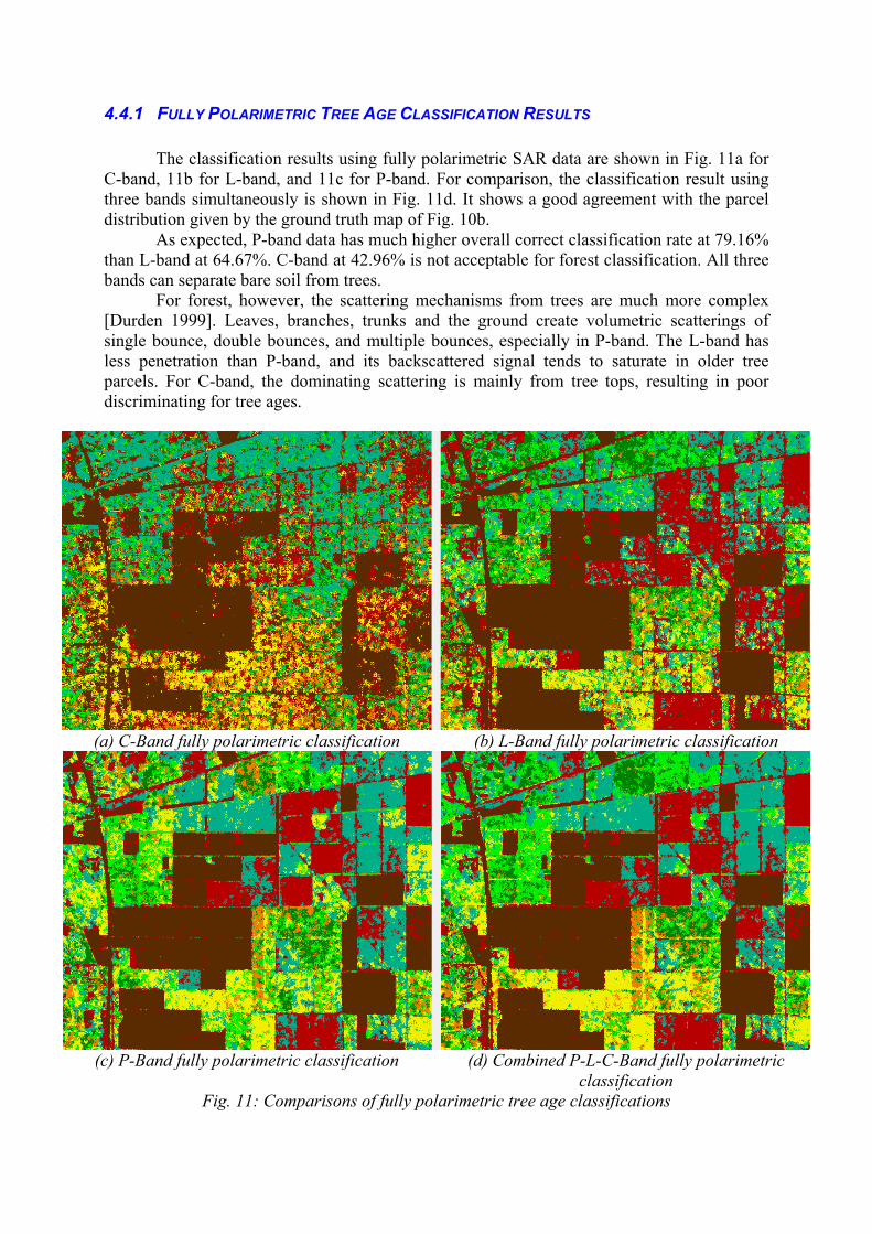
4.4.1 FULLY POLARIMETRIC TREE AGE CLASSIFICATION RESULTS

The classification results using fully polarimetric SAR data are shown in Fig. 11a for C-band, 11b for L-band, and 11c for P-band. For comparison, the classification result using three bands simultaneously is shown in Fig. 11d. It shows a good agreement with the parcel distribution given by the ground truth map of Fig. 10b.

As expected, P-band data has much higher overall correct classification rate at 79.16% than L-band at 64.67%. C-band at 42.96% is not acceptable for forest classification. All three bands can separate bare soil from trees.

For forest, however, the scattering mechanisms from trees are much more complex [Durden 1999]. Leaves, branches, trunks and the ground create volumetric scatterings of single bounce, double bounces, and multiple bounces, especially in P-band. The L-band has less penetration than P-band, and its backscattered signal tends to saturate in older tree parcels. For C-band, the dominating scattering is mainly from tree tops, resulting in poor discriminating for tree ages.

(a) C-Band fully polarimetric classification (b) L-Band fully polarimetric classification

(c) P-Band fully polarimetric classification (d) Combined P-L-C-Band fully polarimetric classification

Fig. 11: Comparisons of fully polarimetric tree age classifications

4.4.2 DUAL POLARIZATION TREE AGE CLASSIFICATION RESULTS

For P-band, the combination of HH and HV performs better than HH and VV as shown in Fig. 12. Phase differences are less influential on the classification, because scattering mechanisms in tree areas are very random. Consequently, phase differences between polarizations are very noisy.

The overall classification accuracy for complex HH and VV of 68.56% is very close to that for HH and VV intensities of 65.30%. This difference is much less than that from crop classification. The complex HH and HV classification accuracy is much higher at 75.95, and the HH and HV intensities is at 75.44%. The difference between using and not using phases is negligible for all three dual polarization modes. We also notice that the use of HH and HV can achieve results nearly as good as that of fully polarimetric SAR. This is because the contribution of HV polarization to tree age classification is the most significant.

Classification for L-band is similar but somewhat inferior. The performance of C-band are much worse due to the inadequate penetration of its shorter wavelength.

(a) P-band complex HH and VV (b) P-band HH and VV intensity (without phase)

(c) P-band complex HH and HV (d) P-band HH and HV intensities (without phase) Fig. 12: Comparisons of dual polarization tree age classifications.

4.4.3 SINGLE POLARIZATION TREE AGE CLASSIFICATION

The overall tree age classification accuracies for single polarization are much better than those for crop classification. P-band HV has the overall classification rate of 68.88%, HH of 58.31%, and VV of 53.89%. Classification rates for single polarization are very close to those for dual polarization for all three bands. It indicates that highly correlated radar returns between polarizations.

Applying target decomposition of Cloude and Pottier [Cloude 1996], to fully polarimetric SAR images, we found that the entropy are very high for all forest areas, revealing random scattering mechanisms. In other words, the backscattered signals are very depolarized; the polarization effect is less significant. Cross-polarization HV produces better classification results than HH and VV, because the volumetric scattering in forest areas enhances the cross-polarization returns. 4.5 CONCLUSION

A procedure has been developed to quantitatively evaluate the classification capabilities for fully polarimetric, combinations of dual polarization and single polarization SAR. Quantitative comparison has been made for crop and forest age classifications for P-band, L-band and C-band frequencies. The fully polarimetric and partially polarimetric classification algorithms are developed based on the principle of maximum likelihood classifier. All probability densities functions are derived from the complex Wishart distribution under the circular Gaussian assumption for single look complex polarimetric data. These optimal classifiers, developed on the same foundation ensure a fair comparison of classification capabilities.

We found that L-band fully polarimetric SAR data are best for crop classification, but P-band is best for forest age classification, because longer wavelength electromagnetic waves provides higher penetration. For dual polarization classification, the HH and VV phase difference is important for crop classification, but less important for tree age classification.

For crop classification, it is clear that the combination of HH and VV polarization is preferred, if fully polarimetric data is not available. The contribution of co-polarization phase differences to classification is highly significant. The classification results using P-band and C-band data are inferior to those using L-band. Also, for crop classification, the L-band complex HH and VV can achieve correct classification rates almost as good as for full polarimetric SAR data, and for forest age classification, P-band HH and HV should be used in the absence of fully polarimetric data.

In all cases, we have demonstrated that multi-frequency fully polarimetric SAR is highly desirable. The methodology introduced in this section should have an impact on the selection of polarizations and frequencies in current and future SAR systems for various applications.

5 UNSUPERVISED POLARIMETRIC CLASSIFICATION

Classification of Earth terrain types within a fully polarimetric SAR image is one of the many important applications of radar polarimetry. Several algorithms have recently been developed for the classification of land features based on their polarimetric microwave signatures. These methods exploit observed similarities and correlation in feature vectors

derived mainly from complete coherent scattering matrix data. Most of these techniques are supervised, in the sense that the feature vector is derived from measurements over known terrain classes. Unknown pixels are then compared with the training set, and a statistical decision is made as to class membership.

When the ground truth is not available, it is often difficult to select significant training sets. Several unsupervised techniques have also been developed. They tend to be more physically based and have the advantage that their performance is not data specific, as often arises with supervised methods. These methods tend to classify automatically the SAR image by finding clusters following a given strategy. Different unsupervised polarimetric classification procedures are outlined and discussed in this section. 5.1 UNSUPERVISED IDENTIFICATION OF A POLARIMETRIC SCATTERING MECHANISM

An unsupervised classification scheme has been introduced [Cloude 1997], based on the use of the two-dimensional H / α classification plane, where all random scattering mechanisms can be represented. The key idea is that entropy arises as a natural measure of the inherent reversibility of the scattering data and that the alpha angle (α) can be used to identify the underlying average scattering mechanisms.

This classification plane is sub-divided into nine basic zones characteristic of classes of different scattering behavior. It is important to note that the absolute magnitude of the eigenvalues were not taken into account. This simple classification procedure was just based on the comparison to fixed thresholds of the polarimetric properties of the different scattering mechanisms. The different class boundaries, in the H-α plane, have been determined so as to discriminate surface reflection (SR), volume diffusion (VD) and double bounce reflection (DB) along the α axis and low, medium and high degree of randomness along the entropy axis. Detailed explanations, examples and comments concerning the different classes can be found in [Cloude 1997].

Fig. 13 shows the H-α plane and the occurrence of the studied polarimetric data into this plane.

Fig. 13: Polarimetric data occurrence in the H-α plane. San Francisco Bay (Left) and Oberpfaffenhofen (right).

It can be seen, in Fig. 13, that the largest densities in the two occurrence planes

correspond to volume diffusion and double bounce scattering with moderate and high randomness. Medium and low entropy surface scattering mechanisms are also frequently encountered in the two scenes under examination. Data distribution in the H-α plane show that identification results may highly depend on segmentation thresholds. Results of this simple unsupervised identification procedure are presented in Fig. 14.

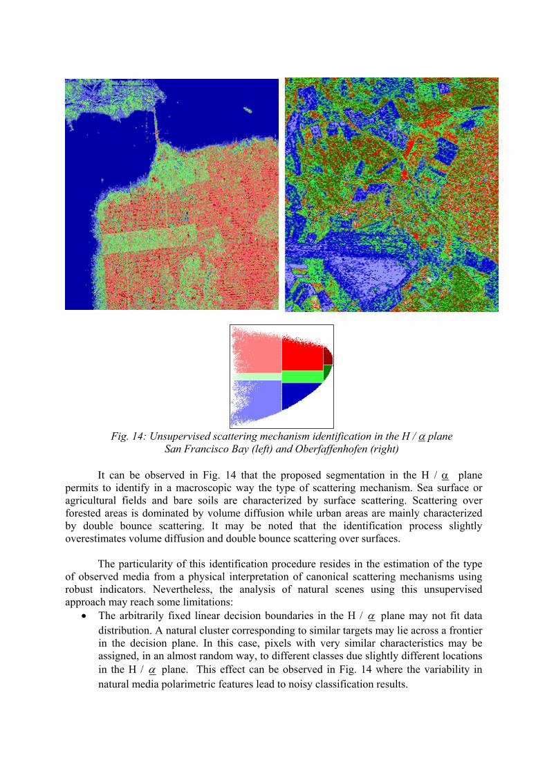
Fig. 14: Unsupervised scattering mechanism identification in the H / α plane

San Francisco Bay (left) and Oberfaffenhofen (right)

It can be observed in Fig. 14 that the proposed segmentation in the H / α plane permits to identify in a macroscopic way the type of scattering mechanism. Sea surface or agricultural fields and bare soils are characterized by surface scattering. Scattering over forested areas is dominated by volume diffusion while urban areas are mainly characterized by double bounce scattering. It may be noted that the identification process slightly overestimates volume diffusion and double bounce scattering over surfaces.

The particularity of this identification procedure resides in the estimation of the type of observed media from a physical interpretation of canonical scattering mechanisms using robust indicators. Nevertheless, the analysis of natural scenes using this unsupervised approach may reach some limitations:

• The arbitrarily fixed linear decision boundaries in the H / α plane may not fit data distribution. A natural cluster corresponding to similar targets may lie across a frontier in the decision plane. In this case, pixels with very similar characteristics may be assigned, in an almost random way, to different classes due slightly different locations in the H / α plane. This effect can be observed in Fig. 14 where the variability in natural media polarimetric features lead to noisy classification results.

• Even if the computation of H and α requires fully polarimetric data, these two parameters do not represent the whole polarimetric information. The use of other indicators such as the span or specific correlations coefficients may improve the classification results in a significant way.

Segmentation procedures based on the whole coherency matrix statistics permit to

overcome the limitations mentioned above. Nevertheless, it is shown in the following, that the physical interpretation of the scattering phenomenon permits to enhance in a significant way the performance of statistical segmentation schemes.

5.1.1 THE COMBINED H / α - WISHART CLASSIFICATION

In 1994, J.S. Lee et al. [Lee 1994a] developed a supervised algorithm based on the complex Wishart distribution for the polarimetric covariance matrix. This algorithm is statistically optimal in that it maximizes the probability density function of pixels' covariance matrices. However, as for all supervised methods, training sets have to be selected in advance. These training sets, selected in advance, require from the user an a priori knowledge of the different significative Earth terrain components which can be found in the POLSAR image.

In 1998, J.S. Lee et al. [Lee 1999b] proposed an unsupervised classification method that uses the two-dimensional H / α classification plane to initially classify the polarimetric SAR image. The initial classification map defines training sets for classification based on the Wishart distribution. The classified results are then used as training sets for the next iteration using the Wishart method. Significant improvement in each iteration has been observed, and the analysis of the final class centers in the two-dimensional H / α classification plane are useful for interpretation of terrain types. The polarimetric H / α segmented image is used as training sets for the initialization of the supervised Wishart classifier. The cluster centers of the coherency matrices, [Tm], is computed for each zone, with :

[ ] [ ]TN

Tmm

kk

k N m

==

=

∑11

(35)

where Nm is the number of pixels in the a priori class ωm. Each pixel in the whole image is then reclassified by applying the distance measure procedure. The reclassified image is then used to update the [Tm], and the image is then again classified by applying the same distance measure procedure. To classify similar objects in the same image, which can have different orientation angles, the orientation dependence is removed from the coherency matrix during the Wishart classification. The classification procedure stops when a termination criterion, defined by the user, is met. The termination criterion we used is the number of iterations and is here equal to 4. In this case, the ratio of pixels switching class with respect to the total pixel number is smaller than 10%. Classification results are shown on Fig. 15 with the corresponding color coded distribution of the data in the two-dimensional H / α.

Fig. 15: Classification result after 4 iterations San Francisco Bay (left) and Oberfaffenhofen (right)

An important improvement in the segmentation accuracy can be observed in the two images presented in Fig. 15. The main kinds of natural media are clearly discriminated by the Wishart H-α segmentation scheme. This unsupervised classification algorithm modifies the decision boundaries in an adaptive way to better fit the natural distribution of the scattering mechanisms and takes into account information related to the back-scattered power.

However, the identification of the terrain type directly from the analysis of the classified image may cause some confusion, due to the color scheme [Lee 1999b]. Indeed, during the classification, the cluster centers in the two-dimensional H / α plane can move out of their zones, or several clusters may end in the same zone [Lee 1999b]. This is due to the fact that the zone boundaries were set somewhat arbitrarily as mentioned previously. It is thus necessary to study the final H / α location of each class to identify the terrain type, and to interpret the scattering mechanisms.

5.1.2 THE COMBINED H / A / α - WISHART CLASSIFICATION In order to improve the capability to distinguish between different classes whose cluster centers end in the same zone, the combined Wishart classifier is extended and complemented with the introduction of the anisotropy (A) information. The original method we proposed, consists in comparing the anisotropy value of all the pixels to ½. This comparison procedure leads to the definition of an « equivalent » projection of the three-dimensional H / A / α space in two complemented H / α planes, as shown on Fig. 16, where is represented the POLSAR data distribution of the San Francisco

bay. The color coding associated to the first 8 classes is retained and 8 new colors are introduced.

Fig. 16a : Distribution of the San-Francisco POLSAR data in the two-dimensional H / α

plane corresponding to A < ½.

Fig. 16b : Distribution of the San-Francisco POLSAR data in the two-dimensional H / α

plane corresponding to A > ½.

A2A1 A4A3

From the analysis of these two complemented H / α planes, it is thus possible to define four main areas (A1 ... A4), each of them gathering several zones (Zi), leading to the following interpretation : 1) - Area 1 (A1) corresponds to the zones where occurs one single scattering mechanism. This is equivalent to the (1-H)(1-A) image. 2) - Area 2 (A2) corresponds to the zones where occurs three scattering mechanisms. This is equivalent to the H(1-A) image. 3) - Area 3 (A3) and Area 4 (A4) correspond to the zones where occur two scattering mechanisms. These are equivalent respectively to the (1-H)A and HA images. Among the different approaches tested, the best way to introduce the anisotropy information in the classification procedure consists in implementing two successive combined Wishart classifiers. The first one is identical to the previous one. Once the first classification procedure has met its termination criterion, the anisotropy comparison for all the pixels, is then introduced, which leads to the definition of 16 new training sets used for the initialization of the second Wishart classifier.

Initialize pixel distributionover 8 classes

85.0 +Χ→Χ⇒> mmA⇒ 16 classes

Anisotropy

Segmented H- planeα

Initialize pixel distributionover 8 classes

Initialize pixel distributionover 8 classes

Initialize pixel distributionover 8 classes

85.0 +Χ→Χ⇒> mmA⇒ 16 classes

85.0 +Χ→Χ⇒> mmA⇒ 16 classes

Anisotropy

Segmented H- planeαSegmented H- planeα

Fig. 17: Synopsis of the Wishart H-A-α segmentation procedure

The entire unsupervised Wishart classification procedure is as follows : 1 : Apply target decomposition to compute the entropy H and α. 2 : First initial classification of the image into 8 classes by zone in the two- dimensional H / α plane. 3 : For each class, compute the initial cluster center [Tm](0) (k=iteration number and m=1..8) 4 : Classify the whole image using the distance measure procedure 5 : Compute [Tm](k+1) for each class using the classified pixels of step 4 6 : Return to step 4, until a termination criterion defined by the user is met. 7 : Apply target decomposition to compute the anisotropy A. 8 : Second initial classification of the image into 16 classes by zone in the projected three-dimensional H / A / α space, with :

if A Class Class

if A Class Classi j i j

Newi j

Old

i j i jNew

i jOld

( , ) ( , ) ( , )

( , ) ( , ) ( , )

.

.

< ⇒ =

< ⇒ = +

0 5

0 5 10 9 : For each class, compute the new initial cluster center [Tm](0) (k=iteration number and m=1..16) 10 : Classify the whole image using the distance measure procedure 11 : Compute [Tm](k+1) for each class using the classified pixels of step 10 12 : Return to step 10, until a termination criterion defined by the user is met.

To compare with the previous procedure, we kept the same termination criterion. The classification results are shown on Fig. 18.

Fig. 18: Classification result after 4 iterations San Francisco Bay (left) and Oberfaffenhofen (right)

Improvements in classification and details are observed. Grass fields are much better defined, and more details are shown both in city blocks and in ocean. Some classes, indistinguishable in the classification based on entropy (H) and alpha angle (α) are now clearly visible with the introduction of the anisotropy information. It is also possible to discriminate different areas, belonging to the same scattering type (same entropy H and alpha angle) but differentiated with the associated anisotropy information which is there significative of the presence of several scattering mechanism types. The analysis of the final cluster centers in the three-dimensional H / A / α classification space will provide a more precise interpretation of the different classes of terrain types.

The segmentation results presented in Fig. 18 show an enhanced description of the Oberpfaffenhofen scene. The introduction of the anisotropy in the clustering process permits to split large segments into smaller clusters discriminating small disparities in a refined way. Several kinds of agricultural fields are separated. The runway and other low intensity targets are distinguished from other surfaces. Buildings are discriminated from other types of scatterers present in urban areas. The Wishart H-A-α classification scheme gathers into segments pixels with similar statistical properties, but does not provide any information concerning the nature of the scattering mechanism associated to each cluster.

The unsupervised classification results show a good discrimination of the three basic scattering mechanisms over the scene under consideration. Forested areas are well separated from the rest of the scene. Buildings, characterized by double bounce scattering, can be

distinguished over the urban area and the DLR. It may be noted that the identification assigns some buildings to the volume diffusion class. The polarimetric properties as well as the power related information do not permit to separate these targets form forests. Such buildings have specific orientations with respect to the radar and particularly rough roofs and back-scatter randomly polarized waves. The information contained in the three roll-invariant parameters extracted from the local estimate of the 3x3 hermitian coherency matrix <[T]>, corresponds to the type of scattering process which occurs inside the pixel to be classified (combination of entropy H and anisotropy A) and to the corresponding physical scattering mechanism (α parameter). From the analysis of the three-dimensional H / A / α classification space, we have shown that the anisotropy can be considered now as a key parameter in the polarimetric analysis and/or inversion of POLSAR data. The analysis of the final cluster centers in the H / A / α classification space is useful for class identification of the different scattering mechanisms which occur in the classified SAR image. The introduction of the anisotropy information improves the capability to distinguish between different classes whose cluster centers end in the same H / α zone.

5.1.3 BASIC IDENTIFICATION OF CANONICAL SCATTERING MECHANISMS

An efficient estimation of the nature of scattering mechanisms over natural scenes can be achieved by gathering results obtained from the polarimetric decomposition and segmentation procedures presented previously. The identification of the polarimetric properties of compactly segmented clusters permits, by analyzing groups of scatterers, to reduce the influence of the variability of polarimetric indicators encountered over natural media. The estimation of global properties provides an accurate interpretation of the observed scene nature and structure. Volume diffusion and double bounce scattering were found to be over-estimated during the identification of scattering mechanisms using the H / α segmented plane. One of the reasons of this over-estimation resides in the calculation of the average parameters of the polarimetric decomposition. In some cases, the expansion of a coherency results a dominant scattering mechanism and secondary mechanism showing very different polarimetric properties.

The calculation of average indicators as the weighted sum of the indicators of each element of the expansion may then lead to an erroneous interpretation of the nature of the scattering mechanism. Recently, a new identification approach was proposed [Ferro-Famil 2002] and based on the discrimination, from the H / A plane, of the number of significant mechanisms occurring in each pixel of the POLSAR image. The relevant mechanisms selection and identification to canonical scattering mechanisms results are shown in Fig. 19.

ODD VOL DBL

Fig. 19: Selection of significant mechanisms and identification to canonical scattering mechanisms (ODD: Single Bounce Scattering, DBL: Double Bounce Scattering, VOL: Volume Diffusion)

This simple and basic identification procedure shows a good discrimination of the three basic scattering mechanisms over the scene under consideration. Forested areas are well separated from the rest of the scene. Buildings, characterised by double bounce scattering, can be distinguished over the urban area and the DLR Institute. It may be noted that the identification assigns some buildings to the volume diffusion class. The polarimetric properties as well as the power related information do not permit to separate these targets form forests. Such buildings, with particularly rough roofs, present specific orientations with respect to the radar line of sight that may cause a random backscattering effect. This limitation can be solved when applying to each canonical scattering mechanism, an unsupervised classification process gathering polarimetric and interferometric results [Ferro-Famil 2002].

This new approach shows significant improvements compared to the strictly polarimetric case. Clear-cuts sparse and dense forests are separated according to their coherent properties and, particular buildings having a polarimetric behaviour similar to forest are then discriminated.

Indeed, interferometric data provide information concerning the coherence of the scattering mechanisms and can be used to retrieve observed media structures and complexity [Cloude 1998, Papathanassiou 2001]. An example of the complementary aspect of polarimetric and interferometric information is given on Fig. 20 with polarimetric interferometric data acquired by the DLR E-SAR sensor at L band in repeat-pass mode with a baseline of 10m.

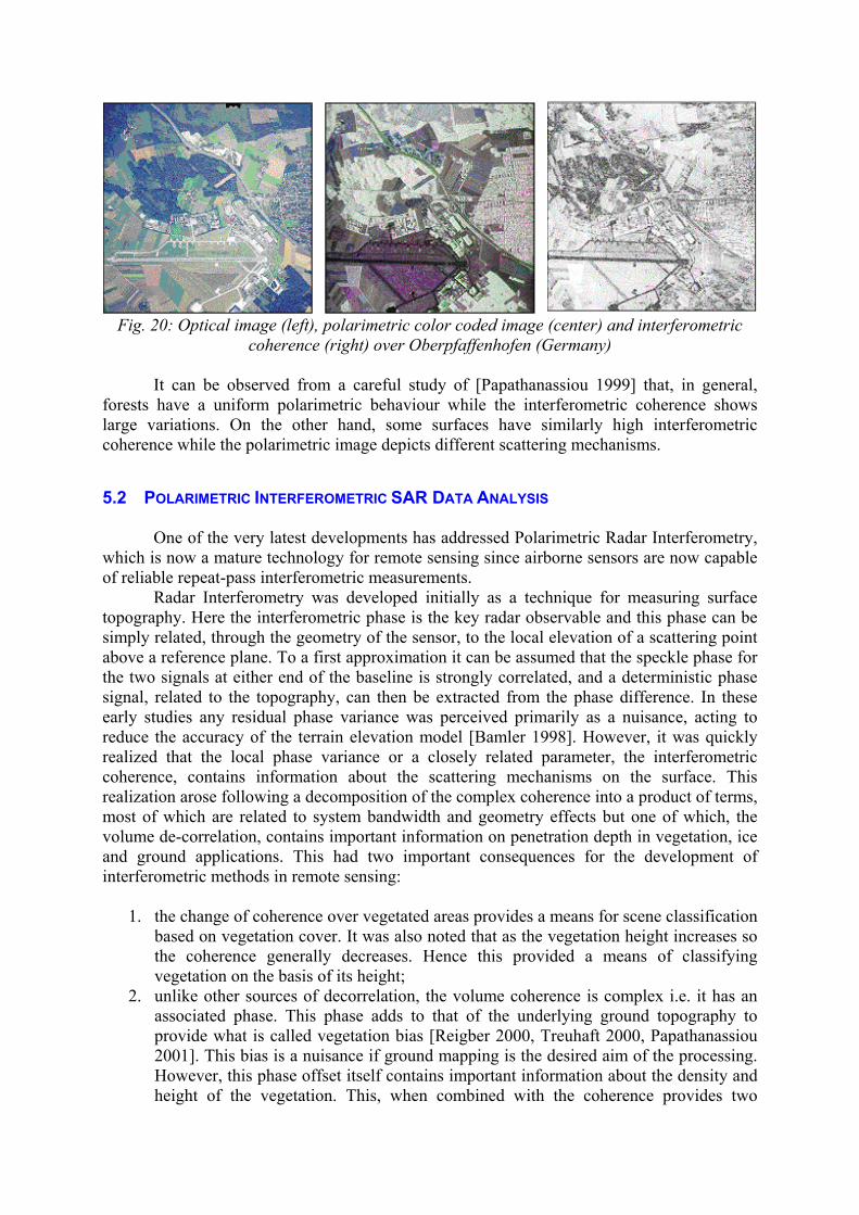
Fig. 20: Optical image (left), polarimetric color coded image (center) and interferometric

coherence (right) over Oberpfaffenhofen (Germany)

It can be observed from a careful study of [Papathanassiou 1999] that, in general, forests have a uniform polarimetric behaviour while the interferometric coherence shows large variations. On the other hand, some surfaces have similarly high interferometric coherence while the polarimetric image depicts different scattering mechanisms.

5.2 POLARIMETRIC INTERFEROMETRIC SAR DATA ANALYSIS

One of the very latest developments has addressed Polarimetric Radar Interferometry, which is now a mature technology for remote sensing since airborne sensors are now capable of reliable repeat-pass interferometric measurements.

Radar Interferometry was developed initially as a technique for measuring surface topography. Here the interferometric phase is the key radar observable and this phase can be simply related, through the geometry of the sensor, to the local elevation of a scattering point above a reference plane. To a first approximation it can be assumed that the speckle phase for the two signals at either end of the baseline is strongly correlated, and a deterministic phase signal, related to the topography, can then be extracted from the phase difference. In these early studies any residual phase variance was perceived primarily as a nuisance, acting to reduce the accuracy of the terrain elevation model [Bamler 1998]. However, it was quickly realized that the local phase variance or a closely related parameter, the interferometric coherence, contains information about the scattering mechanisms on the surface. This realization arose following a decomposition of the complex coherence into a product of terms, most of which are related to system bandwidth and geometry effects but one of which, the volume de-correlation, contains important information on penetration depth in vegetation, ice and ground applications. This had two important consequences for the development of interferometric methods in remote sensing:

1. the change of coherence over vegetated areas provides a means for scene classification

based on vegetation cover. It was also noted that as the vegetation height increases so the coherence generally decreases. Hence this provided a means of classifying vegetation on the basis of its height;

2. unlike other sources of decorrelation, the volume coherence is complex i.e. it has an associated phase. This phase adds to that of the underlying ground topography to provide what is called vegetation bias [Reigber 2000, Treuhaft 2000, Papathanassiou 2001]. This bias is a nuisance if ground mapping is the desired aim of the processing. However, this phase offset itself contains important information about the density and height of the vegetation. This, when combined with the coherence provides two

parameters which are directly related to the vertical structure of the vegetation cover on the surface [Cloude 1998, Treuhaft 2000, Papathanassiou 2001, Yamada 2001].

The structure of vegetation is a key ecosystem factor that reflects biomass stock

successions and growth dynamics. Parameters such as tree height, crown width, stand and canopy density and the underlying ground topography are direct inputs into biomass determination models and enable ecological process modelling, forest inventory and predictive modelling in hydrology. It should also be pointed out that global forest inventory and forest (above ground) biomass are currently critical missing parts in the global climate change debate. Hence there is a need for a reliable remote sensing technique to provide such information, and for developing alternate POLInSAR feature extraction algorithms such as that of [Yamada 2001].

By operating at longer wavelengths such as L and P bands, Polarimetric Radar Interferometry [Cloude 1998, Papathanassiou 2001] is well suited to this problem as it provides penetration into vegetation cover and the ground and hence is inherently sensitive to volume effects and provides vertical structure information on a scale not easily available from optical or laser sensors. This technology promises to provide the basis for important new radar remote sensing instruments for global biomass and vegetation mapping [Mette 2002].

5.2.1 POLARIMETRIC INTERFEROMETRIC COHERENCE OPTIMISATION PROCEDURE

Polarimetric Radar Interferometry is a sensor technology measuring the full scattering matrix at either end of the baseline [Bamler 1998, Cloude 1998, Treuhaft 2000, Yamada 2001]. The polarimetric interferometric behaviour of a target is then fully described by the two scattering matrices, [S1] and [S2], and a six element complex target vector, k6, can be obtained by stacking target vectors from each polarimetric image, gathers the polarimetric interferometric information into a compact representation [Cloude 1998, Papathanassiou 2001]. The corresponding 6×6 interferometric coherency matrix is given by:

[ ] ∑=n

†666 kk

n1T with

=

2

16 k

kk and [ ]T

3i2i1ii k,k,kk = (36)

This coherency matrix has the following structure:

[ ] [ ] [ ][ ] [ ]

=

22†12

12116 T

TT

ΩΩ

with [ ] ∑=n

†2112 kk

n1Ω (37)

The leading diagonal blocks are the conventional hermitian coherency matrices. In

applications interest centres on exploitation of the off diagonal block [Ω12] which is the 3x3 complex polarimetric cross-correlation matrix. As the target vector k6 follows a complex normal zero mean distribution [ ]( )6C ,0N Σ , with [ ]6Σ its 6x6 covariance matrix, the 6x6 coherency matrix [Τ6] has then a complex Wishart distribution [ ]( )6C ,0W Σ , characterised by n degrees of freedom [Ferro-Famil 2001a, Ferro-Famil 2001b]. The interferometric cross-correlation matrix, [Ω12], has complex diagonal elements, from which is computed the three polarimetric complex coherences as follows:

),,( 321 γγγ with *

i2i2*i1i1

*i2i1j

iikkkk

kke~ i == φγγ (38)

where the operator < > stands for the averaging over n samples. Standard real coherence values are obtained from iγ , while the arguments correspond to the interferometric phase difference. It may be noted that the coherence defined in (37) is not invariant under a change of polarimetric basis. In general, coherence may be decomposed into multiplicative contributions as [Cloude 1998, Papathanassiou 2001]:

polartemporalspatialSNR~.~.~.~~ γγγγγ = (39)

where the different terms indicate decorrelations related respectively to the back-scattered wave signal to noise ration, the spatial distribution of the illuminated scatterers, temporal variations between the acquisitions and finally the polarization state. Coherence images for the different polarization channels are displayed in Fig. 21.

1γ 2γ 3γ

0 0.5 10 0.50 0.5 11

Fig. 21: Interferometric coherences for the different polarimetric channels in the Pauli basis

Range filtering and topographic phase removal procedures are applied to the interferometric data sets prior to the computation of the polarimetric interferometric coherences. The range filtering procedures corrects wave number shifts inherent to interferometric measurements. High coherence values are observed for surface areas in the co-polarized channels. Smooth surfaces, like the runway, scatter waves in the radar direction with a low signal to noise ratio, involving a low coherence in every polarization channel. In a general way, the maximum of the three coherence set corresponds to the first or second channel according to the dominant scattering mechanism, i.e. single or double bounce reflection respectively. Over forested areas, all three coherencies have low values.

The off-diagonal complex polarimetric cross-correlation matrix [Ω12] contains low variance differential phase information related to the height separation of scattering centres. Rather than fusing the two data sets, Cloude and Papathanassiou [Cloude 1998, Papathanassiou 2001] have introduced polarization filters that minimize the variance of this phase information to locate as accurately as possible the position of the scattering centre. With full polarimetric interferometry it is then possible to select in the post processing the w

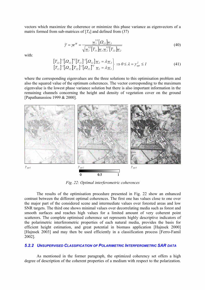
vectors which maximize the coherence or minimize this phase variance as eigenvectors of a matrix formed from sub-matrices of [T6] and defined from (37)

[ ]

[ ] [ ] 222T*

2111T*

1

212T*

1i

wTwwTw

wwe~ Ωγγ φ == (40)

with: [ ] [ ] [ ] [ ][ ] [ ][ ] [ ]

10 ww TTww TT 2

opt11

T*12

12212

111

22121

11T*

121

22 ≤=≤⇒

==

−−

−−

γλλΩΩλΩΩ (41)

where the corresponding eigenvalues are the three solutions to this optimisation problem and also the squared value of the optimum coherences. The vector corresponding to the maximum eigenvalue is the lowest phase variance solution but there is also important information in the remaining channels concerning the height and density of vegetation cover on the ground [Papathanassiou 1999 & 2000].

1optγ 2optγ 3optγ

0 0.5 10 0.50 0.5 11

Fig. 22: Optimal interferometric coherences

The results of the optimisation procedure presented in Fig. 22 show an enhanced contrast between the different optimal coherences. The first one has values close to one over the major part of the considered scene and intermediate values over forested areas and low SNR targets. The third one shows minimal values over decorrelating media such as forest and smooth surfaces and reaches high values for a limited amount of very coherent point scatterers. The complete optimised coherence set represents highly descriptive indicators of the polarimetric interferometric properties of each natural media, provides the basis for efficient height estimation, and great potential in biomass application [Hajnsek 2000] [Hajnsek 2003] and may then be used efficiently in a classification process [Ferro-Famil 2002].

5.2.2 UNSUPERVISED CLASSIFICATION OF POLARIMETRIC INTERFEROMETRIC SAR DATA

As mentioned in the former paragraph, the optimized coherency set offers a high degree of description of the coherent properties of a medium with respect to the polarization.

The color-coded image presented in Fig. 23 represents the joint information associated to the optimal coherencies.

1optγ 1optγ1optγ 1optγ

Fig. 23: Color-coded image of the optimal coherence set

1optγ 1optγ

The color-coding used for the joint representation of the optimal coherency set reveals

particular behaviors of different types of natural medium under examination: • White areas indicate targets showing high coherence independently of the

polarization. Such a behavior is characteristic of point scatterers and bare soils and corresponds, in the Oberpfaffenhofen scene, to buildings, fences and some vegetation free agricultural fields.

• Green zones reveal the presence of a single dominant coherent mechanism within the resolution cell. Secondary coherences, associated to the red and blue channels have significantly lower values. Such zones correspond to surfaces with low SNR responses and some particular fields.

• Forested areas, characterized by a dark green color have scattering features dominated by a single mechanism but with a very low coherence.

• A comparison of the image of Fig. 23 with the polarimetric color-coded image shown in Fig. 20 indicates that the distribution of strictly polarimetric and polarimetric interferometric features over surfaces and agricultural fields are significantly different. Coherence related information permits to discriminate particular buildings that cannot be separated from forested areas using only polarimetric data.

• Over forested areas, the polarimetric color-coded image shows homogeneous zones, while interferometric data indicate that there exist large variations of the coherent scattering properties corresponding to clear-cuts and low-density forest.

In order to isolate the polarization dependant part of the optimal coherencies, it is necessary to define their relative values as:

∑= joptioptiopt γγγ /~ with 321~~~

optoptopt γγγ ≥≥ (42)

The relative optimal coherence spectrum can be fully described by two parameters. We propose to define A1 and A2 as characteristic indicators of the distribution of the coherency in the different optimized channels.

1

211 ~

~~

opt

optoptAγ

γγ −= and

1

312 ~

~~

opt

optoptAγ

γγ −= (43)

These parameters indicate relative amplitude variations between the different optimized channels. Similarly to the polarimetric case, the indicators A1 and A2 may be used to estimate the number of independent coherent scattering mechanisms from the optimization results. The different optimal coherence set configurations are represented and identified in Fig. 24.

A2

A1

N/A N/A

N/A

0.5 A10.9 1

0.5

1

0

A2A2

A1

N/A N/A

N/A

A2

A1

N/A N/A

N/A

0.5 A10.9 1

0.5

1

0

A2

0.5 A10.9 1

0.5

1

0

A2

Fig. 24: Discrimination of different optimal coherence set using A1 and A2 (left).

Selection in the A1-A2 plane (right).

The schematic on the left hand side of Fig. 24 separates the different optimal coherence set configurations in five classes. The diagonal classes correspond to configurations for which 32

~~optopt γγ =

1

with different importance with respect to the largest normalized coherence ~

optγ . A column describes configurations with a constant proportionality ratio between 2

~optγ and 1

~optγ . The real segmentation from A1 and A2 is

realized over nine classes in order to improve the resulting clusters descriptivity and accuracy. Results of the normalized optimal coherence set classification are shown in Fig. 25.

Approximately four major classes arise from the identification of the optimal coherence

set distribution. This unsupervised segmentation was also found to achieve a high degree of descriptivity on other scenes observed with different baselines [Ferro-Famil 2002]. This is due to the fact that it is based on indicators having a reduced sensitivity to decorrelation terms not related to the polarization.

The classification results are used to provide an adequate initialization to a segmentation merging polarimetric and interferometric analysis results. In this way, an unsupervised Maximum Likelihood classification is applied independently on the different types of basic scattering mechanisms identified with polarimetric data. Results for the Volume Diffusion and Surface Reflection classes are shown in Fig. 26.

Fig. 25: Unsupervised identification of the number of coherent scattering mechanisms.

Fig. 26: Unsupervised polarimetric interferometric segmentation results over the Volume Diffusion

basic class (left) and Surface Reflection class (right)

Clusters resulting from the ML segmentation are assigned a color indicating their average coherence, ranging from black for low coherence to white for high coherence.

Globally, polarimetric interferometric characteristics are efficiently segmented into compact clusters corresponding to scatterers with similar polarimetric and interferometric characteristics.

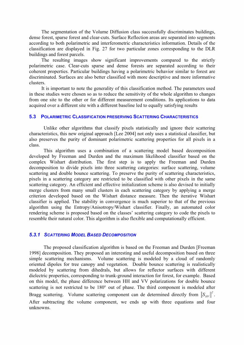
The segmentation of the Volume Diffusion class successfully discriminates buildings, dense forest, sparse forest and clear-cuts. Surface Reflection areas are separated into segments according to both polarimetric and interferometric characteristics information. Details of the classification are displayed in Fig. 27 for two particular zones corresponding to the DLR buildings and forest parcels.

The resulting images show significant improvements compared to the strictly polarimetric case. Clear-cuts sparse and dense forests are separated according to their coherent properties. Particular buildings having a polarimetric behavior similar to forest are discriminated. Surfaces are also better classified with more descriptive and more informative clusters.

It is important to note the generality of this classification method. The parameters used in these studies were chosen so as to reduce the sensitivity of the whole algorithm to changes from one site to the other or for different measurement conditions. Its applications to data acquired over a different site with a different baseline led to equally satisfying results 5.3 POLARIMETRIC CLASSIFICATION PRESERVING SCATTERING CHARACTERISTICS

Unlike other algorithms that classify pixels statistically and ignore their scattering characteristics, this new original approach [Lee 2004] not only uses a statistical classifier, but also preserves the purity of dominant polarimetric scattering properties for all pixels in a class.

This algorithm uses a combination of a scattering model based decomposition developed by Freeman and Durden and the maximum likelihood classifier based on the complex Wishart distribution. The first step is to apply the Freeman and Durden decomposition to divide pixels into three scattering categories: surface scattering, volume scattering and double bounce scattering. To preserve the purity of scattering characteristics, pixels in a scattering category are restricted to be classified with other pixels in the same scattering category. An efficient and effective initialization scheme is also devised to initially merge clusters from many small clusters in each scattering category by applying a merge criterion developed based on the Wishart distance measure. Then the iterative Wishart classifier is applied. The stability in convergence is much superior to that of the previous algorithm using the Entropy/Anisotropy/Wishart classifier. Finally, an automated color rendering scheme is proposed based on the classes’ scattering category to code the pixels to resemble their natural color. This algorithm is also flexible and computationally efficient.

5.3.1 SCATTERING MODEL BASED DECOMPOSITION

The proposed classification algorithm is based on the Freeman and Durden [Freeman 1998] decomposition. They proposed an interesting and useful decomposition based on three simple scattering mechanisms. Volume scattering is modeled by a cloud of randomly oriented dipoles for tree canopy and vegetation. Double bounce scattering is realistically modeled by scattering from dihedrals, but allows for reflector surfaces with different dielectric properties, corresponding to trunk-ground interaction for forest, for example. Based on this model, the phase difference between HH and VV polarizations for double bounce scattering is not restricted to be 180° out of phase. The third component is modeled after Bragg scattering. Volume scattering component can de determined directly from 2

HVS . After subtracting the volume component, we ends up with three equations and four unknowns.

Polarimetric color coded image

Optimal coherence set color coded image

Volume diffusion classification results

Surface reflection classification results

Classification into three canonical mechanisms

including double bounce reflection

Fig. 27: Polarimetric Interferometric classification results over two areas.

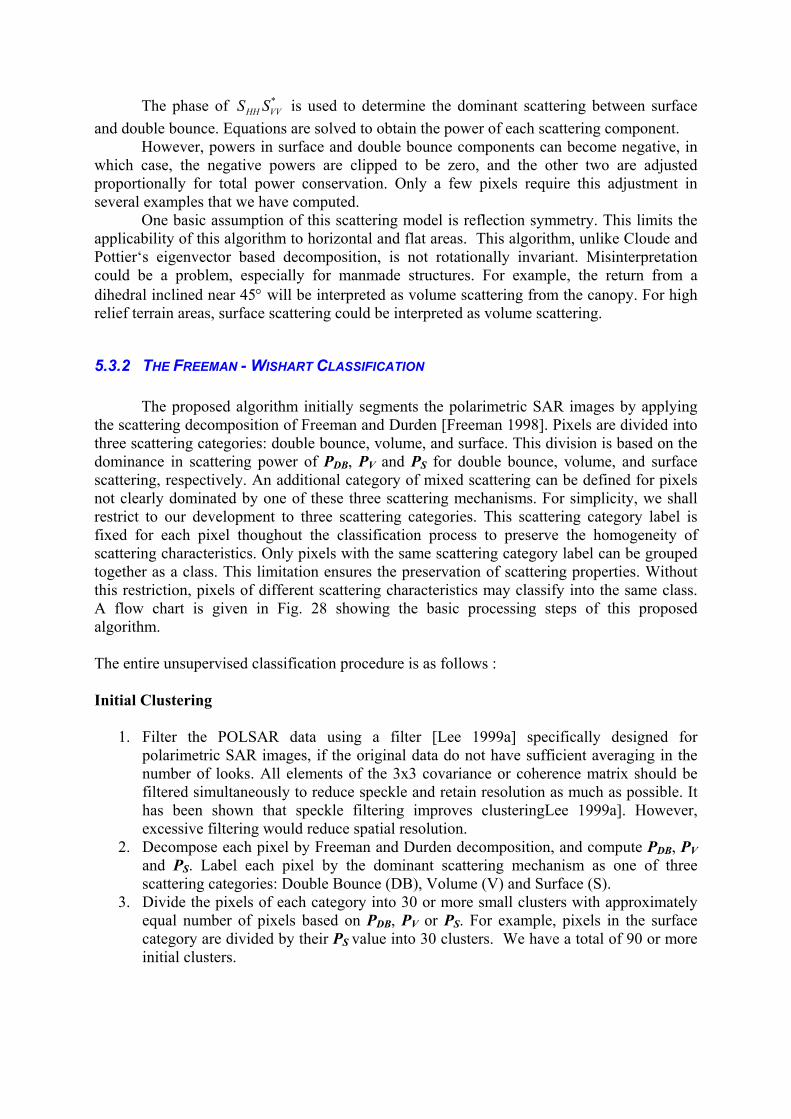
The phase of is used to determine the dominant scattering between surface and double bounce. Equations are solved to obtain the power of each scattering component.

*VVHH SS

However, powers in surface and double bounce components can become negative, in which case, the negative powers are clipped to be zero, and the other two are adjusted proportionally for total power conservation. Only a few pixels require this adjustment in several examples that we have computed.

One basic assumption of this scattering model is reflection symmetry. This limits the applicability of this algorithm to horizontal and flat areas. This algorithm, unlike Cloude and Pottier‘s eigenvector based decomposition, is not rotationally invariant. Misinterpretation could be a problem, especially for manmade structures. For example, the return from a dihedral inclined near 45° will be interpreted as volume scattering from the canopy. For high relief terrain areas, surface scattering could be interpreted as volume scattering.

5.3.2 THE FREEMAN - WISHART CLASSIFICATION

The proposed algorithm initially segments the polarimetric SAR images by applying the scattering decomposition of Freeman and Durden [Freeman 1998]. Pixels are divided into three scattering categories: double bounce, volume, and surface. This division is based on the dominance in scattering power of PDB, PV and PS for double bounce, volume, and surface scattering, respectively. An additional category of mixed scattering can be defined for pixels not clearly dominated by one of these three scattering mechanisms. For simplicity, we shall restrict to our development to three scattering categories. This scattering category label is fixed for each pixel thoughout the classification process to preserve the homogeneity of scattering characteristics. Only pixels with the same scattering category label can be grouped together as a class. This limitation ensures the preservation of scattering properties. Without this restriction, pixels of different scattering characteristics may classify into the same class. A flow chart is given in Fig. 28 showing the basic processing steps of this proposed algorithm. The entire unsupervised classification procedure is as follows : Initial Clustering

1. Filter the POLSAR data using a filter [Lee 1999a] specifically designed for polarimetric SAR images, if the original data do not have sufficient averaging in the number of looks. All elements of the 3x3 covariance or coherence matrix should be filtered simultaneously to reduce speckle and retain resolution as much as possible. It has been shown that speckle filtering improves clusteringLee 1999a]. However, excessive filtering would reduce spatial resolution.

2. Decompose each pixel by Freeman and Durden decomposition, and compute PDB, PV and PS. Label each pixel by the dominant scattering mechanism as one of three scattering categories: Double Bounce (DB), Volume (V) and Surface (S).

3. Divide the pixels of each category into 30 or more small clusters with approximately equal number of pixels based on PDB, PV or PS. For example, pixels in the surface category are divided by their PS value into 30 clusters. We have a total of 90 or more initial clusters.

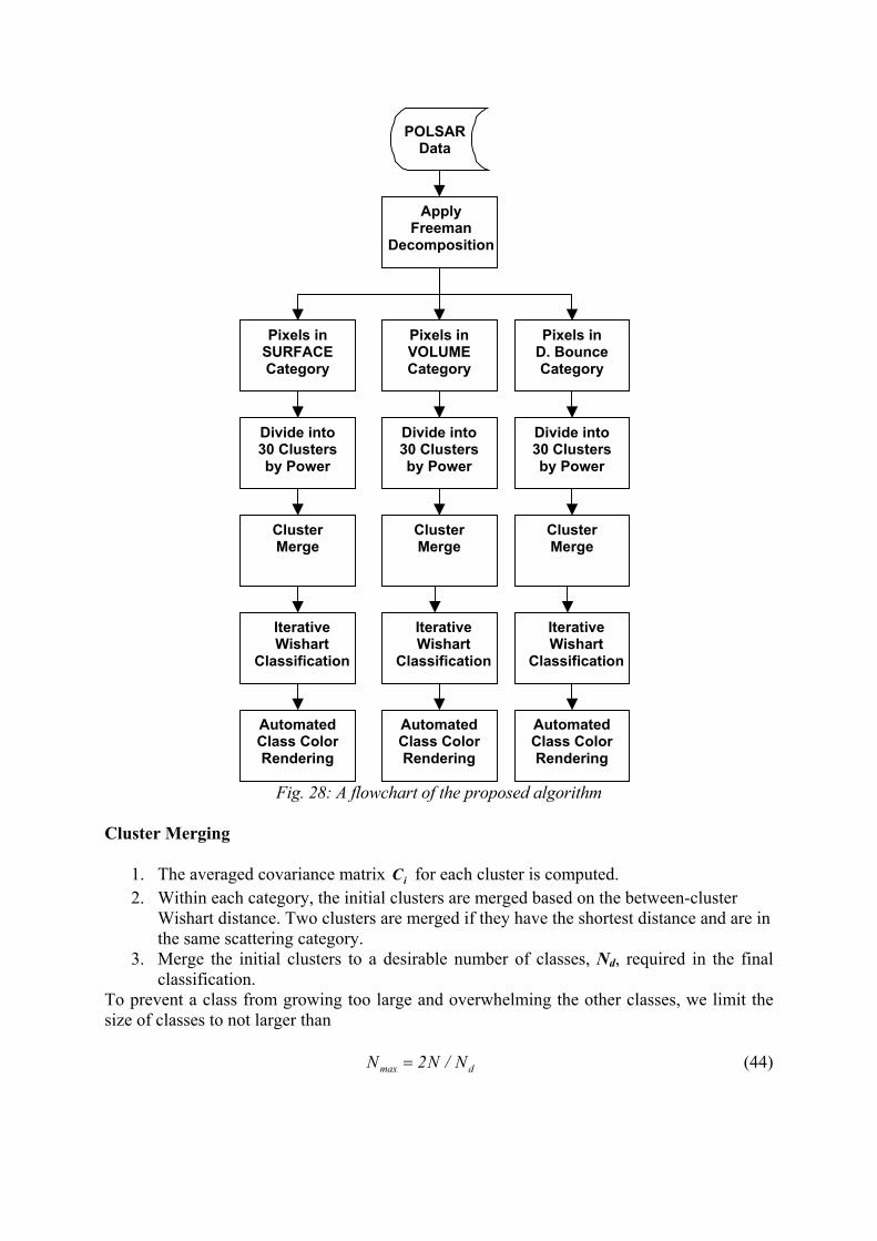
POLSAR Data

Apply Freeman

Decomposition

Pixels in SURFACE Category

Pixels in VOLUME Category

Pixels in D. Bounce Category

Divide into 30 Clusters by Power

Cluster Merge

Divide into 30 Clusters by Power

Iterative Wishart

Classification

Divide into 30 Clusters by Power

Automated Class Color Rendering

Cluster Merge

Iterative Wishart

Classification

Automated Class Color Rendering

Cluster Merge

Iterative Wishart

Classification

Automated Class Color Rendering

Fig. 28: A flowchart of the proposed algorithm

Cluster Merging

1. The averaged covariance matrix C for each cluster is computed. i

2. Within each category, the initial clusters are merged based on the between-cluster Wishart distance. Two clusters are merged if they have the shortest distance and are in the same scattering category.

3. Merge the initial clusters to a desirable number of classes, Nd, required in the final classification.

To prevent a class from growing too large and overwhelming the other classes, we limit the size of classes to not larger than

dmax N/N2N = (44)

N is the total number of pixels in the image. In addition, small clusters are merged first, and only clusters in the same scattering category can be merged to preserve the purity of scattering characteristics. In terrain classification, the number of pixels dominated by double bounce is much smaller than those with surface and volume scattering.

For better separation of pixels in the double bounce category with smaller number of pixels, we limit the merging to at least three final clusters (classes) for each scattering category.

Wishart Classification

1. Compute the averaged covariance matrices from the Nd classes, and use these matrices as the class centers. All pixels are reclassified based on their Wishart distance measure from class centers. Pixels labeled as “DB”, “V” or “S” can only be assigned to the classes with the same label. This ensures the classes are homogeneous in scattering characteristics. For example, a double bounce dominated pixel will not be assigned to a surface scattering class even if the Wishart distance is the shortest.

2. Iteratively apply the Wishart classifier for 2 to 4 iterations with the category restriction for better convergence. The convergence stability is much better than when using the initial clustering from the entropy/α decomposition [Lee 1999b].

Automated Color Rendering

Color coding for each class is important for visual evaluation of classification results. The classes can be easily color-coded by their scattering label.

After the final classification, the color selection for each class is automatically assigned: blue colors for the surface scattering classes, green colors for volume scattering classes, and red colors for double bounce classes. In the surface scattering classes, the class with highest power will be assigned color white to designate the near specular scattering class. The shade of each color is assigned in order of increasing brightness corresponding to the averaged power of the class within its category. For inland scenes, it may be preferable to color the surface classes with brown colors than with blue colors.

It should be noted that identification of classes for terrain types based on scattering mechanisms has to be done carefully. For example, very rough surface can induce volume scattering in Freeman and Durden decomposition. Positive identification of terrain type may require additional contexture information and human reasoning.

5.3.3 EXPERIMENTAL RESULTS

Two examples are given in this section to illustrate the effectiveness of this classification algorithm. A NASA/JPL AIRSAR L-band data of San Francisco are used to show the applicability of this algorithm for general terrain classification using the original data. The original POLSAR image is displayed in Fig. 29a, with Pauli matrix components: |HH-VV|, |HV| and |HH+VV|, for the three composite colors: red, green and blue, respectively. The Freeman decomposition using |PDB|, |PV| and |PS| for red, green and blue is shown in Fig. 29b. The Freeman decomposition possesses similar characteristics to the Pauli-based decomposition, but Freeman decomposition provides a more realistic representation, because it uses scattering models with dielectric surfaces.

(a) Original image

|HH-VV|, |HV|, |HH+VV| (b) Freeman decomposition

|PDB|, |PV|, |PS|

Fig. 29: The characteristics of NASA JPL POLSAR image of San Francisco

After the decomposition, the powers PDB, PV and PS are computed for each pixel. Pixels are categorized as “DB”, “V” and “S” associated with the maximum power of these three scattering mechanisms. Fig. 30a shows the scattering category map with the red color for double bounce scattering, the green color for the volume scattering, and the blue color for the surface scattering. For each scattering category, we divide pixels into 30 clusters based on its power, and then the merge criterion is applied to merge into the pre-selected number of 15 classes. The merged result is shown in Fig. 30b, each class is color coded with the color map in Fig. 31b. Without further applying the iteration of Wishart classifier, this classification result up to this step is much better than that obtained based on the H / α - Wishart classification [Lee 1999b]. This clearly shows the effectiveness of the merge criterion.

After the cluster merge into 15 classes, the Wishart classifier was iteratively applied. The classification results before the iteration (Fig. 30b) looks very similar to those after the fourth iteration (Fig. 31a), indicating good convergence stability. Fig. 31b shows the automated color-coded label for the 15 classes. We have 9 classes with surface scattering because of the large ocean area in the image. As shown in Fig. 31a, details in the ocean areas are enhanced compared with previous classification algorithms. The surface class with the highest returns is colored white, showing pixels with near-specular scattering. This class includes the ocean surface at the top right area because of small incidence angles, and parts of the mountain and coast that are facing the radar look direction. We also observe many specular returns in the city blocks. Three volume classes detail volume scattering from trees and vegetation. The double bounce classes clearly show the street patterns associated with city blocks, and double bounce classes are also scattered through the park areas, probably associated with man-made structures and trunk-ground interactions. It is interesting to compare the classified result (Fig. 31a) with the original image (Fig. 29a). The classified image with 15 classes reveals distinctively more terrain information than the original image.

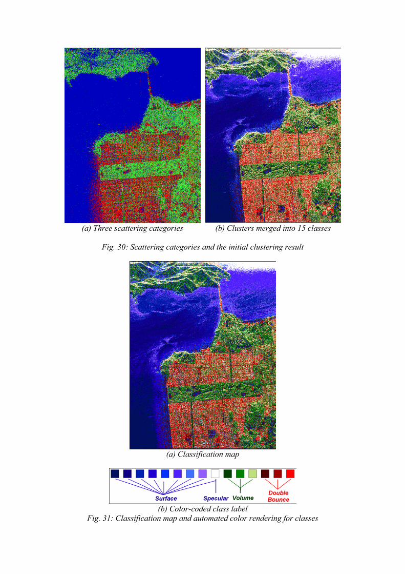
(a) Three scattering categories (b) Clusters merged into 15 classes

Fig. 30: Scattering categories and the initial clustering result

(a) Classification map

(b) Color-coded class label

Fig. 31: Classification map and automated color rendering for classes

We also applied this algorithm to a DLR E-SAR L-Band image of Oberpfaffenhofen,

Germany to demonstrate its effectiveness for a large and high resolution POLSAR image. The original data is in the single-look complex format. The Freeman decomposition is shown in Fig. 32a, which reveals airport runways in the middle with very low radar return, and a forested area in the upper right of the image. We also observe that a few buildings can be mistakenly identified as volume scattering, because they are not directly facing the radar, inducing higher HV returns. The scattering category map in Fig. 32b shows the surface scattering pixels in blue, the volume scattering pixels in green and the double bounce pixels in red. A large number of pixels are categorized as surface scattering, including the runways. However, noisy pixels of volume and double bounce are scattered among the surface pixels, probably due to the inhomogeneity of grass areas, and the low signal-to-noise ratio associated with very low radar returns.

(a) Freeman decomposition |PDB|, |PV|, |PS|

(b) Three scattering categories |DBL|, |VOL|, |ODD|

Fig.32 The characteristics of DLR E-SAR image of Oberpfaffenhofen

The classification map of 16 classes is shown in Fig. 33a with the class label in Fig.

33b. Here, we applied a different color-coding for classes in the surface scattering category. We use the brown colors to better represent the nature of this image because of the absence of any large body of water. The vegetation and forest are well classified. The surface scattering classes show great distinction in separating runways, grass, and plowed fields. To examine in detail, we can show an area around the runway (Fig. 33b), that there exist five trihedrals in the triangle inside the runway which are clearly classified in the specular scattering class shown in white. It is well-known that trihedrals have the same polarimetric signature as specular scattering. Several double bounce reflectors have also been correctly classified near the triangle. Some of the buildings are not classified as double bounce scattering, because they are not aligned facing the radar, and do not induce double bounce returns. We also observed that fences facing the radar are classified as double bounce, but the section aligned at an angle is classified as volume scattering.

To properly classify buildings, interferometric data may be required to separate buildings from vegetation. Buildings tend to have much higher interferometric coherence than vegetation.

(a) Classification map

(b) Color-coded class label

Fig. 33: Classification map and automated color rendering for classes

In this section was presented a very recent and robust classification algorithm that has

better stability in convergence and preserves the homogeneous scattering mechanism of each class. This new algorithm is also flexible in choosing the number of classes, and preserving the spatial resolution in classification results. The initialization procedure is also efficient and quite different from that based on Cloude and Pottier’s decomposition [Lee 1999b][Pottier 2000][Ferro-Famil 2001a][Ferro-Famil 2001c]. The first step is to divide image pixels into three categories by surface, volume and even bounce scattering, by applying the Freeman and Durden decomposition [Freeman 1998]. Pixels in each category are classified independent of pixels in the other categories to preserve the purity of scattering characteristics for each class. A new and effective initialization scheme is also devised to initially merge clusters by applying a criterion developed based on the Wishart distance measure [Lee 1999b]. Pixels are then iteratively classified by the Wishart classifier using the initial clusters as the training sets within each scattering category. For example, pixels in the double bounce category are not allowed to be reclassified into another category. In addition, in order to produce an informative classification map, class color selection is important, so we have developed a

procedure that automatically colors the classification map using scattering characteristics, categorized as surface scattering, double bounce scattering, and volume scattering.

6 REFERENCES [Bamler 1998] R. Bamler, P. Hartl, “Synthetic Aperture Radar Interferometry”, Inverse Problems, 14, R1-R54, 1998. [Boerner 1998] W. M. Boerner et al “Polarimetry in Remote Sensing: Basic and Applied Concepts”, Chapter 5 in Manual of Remote Sensing, Vol. 8, 3rd edition, F M Henderson, A J Lewis eds. New York, Wiley, 1998. [Boerner 2000] W.M. Boerner, Y. Yamaguchi, "Extra Wideband Polarimetry, Interferometry and Polarimetric Interferometry in Synthetic Aperture Remote Sensing", Special Issue on Advances in Radar Systems, IEICE Trans. Commun., Vol. E83-B (9), Sept. 2000, pp 1906-1915. [Chen 1996] K.S. Chen, W.P Huang, D. H. Tsay, F. Amar, "Classification of Multifrequency Polarimetric SAR Image Using a Dynamic Learning Neural Network," IEEE Transactions on Geoscience and Remote Sensing, vol. 34, no.3, 814-820, 1996. [Cloude 1986] S.R. Cloude « Group theory and polarization algebra », OPTIK, vol. 75, n°1, pp 26-36, 1986. [Cloude 1992] S.R. Cloude « Uniqueness of target decomposition theorems in radar polarimetry », Direct and Inverse Methods in Radar Polarimetry, Part 1, NATO-ARW, W.M. Boerner et al., Eds. New York : Kluwer Academic, 1992, pp 267-296. [Cloude 1995] S.R. Cloude « Symmetry, Zero Correlations and Target Decomposition Theorems », Proceedings of 3rd International Workshop on Radar Polarimetry (JIPR '95), IRESTE, University of Nantes, March 1995, pp 58-68. [Cloude 1996] S.R. Cloude, E. Pottier, "A Review of Target Decomposition Theorems in Radar Polarimetry", IEEE Transactions on Geoscience and Remote Sensing, Vol. 34 No. 2, pp 498-518, March 1996. [Cloude 1997] S.R. Cloude, E. Pottier, "An Entropy Based Classification Scheme for Land Applications of Polarimetric SAR", IEEE Transactions on Geoscience and Remote Sensing, Vol. 35, No. 1, pp 68-78, January 1997. [Cloude 1998] S.R. Cloude, K.P. Papathanassiou, “Polarimetric SAR Interferometry”, IEEE Transactions on Geoscience and Remote Sensing, Vol 36. No. 5, pp 1551-1565, September 1998. [Cloude 1999] S.R. Cloude, J. Fortuny, J.M. Lopez, A.J. Sieber, “Wide Band Polarimetric Radar Inversion Studies for Vegetation Layers”, IEEE Transactions on Geoscience and Remote Sensing, Vol 37/2 No 5, pp 2430-2442, September 1999.

[Cloude 2000a] S.R. Cloude, K P Papathanassiou, W M Boerner, “The Remote Sensing of Oriented Volume Scattering Using Polarimetric Radar Interferometry”, Proceedings of International Symposium on Antennas and Propagation, ISAP 2000, Fukuoka, Japan, pp 549-552, August 2000. [Cloude 2000b] S.R. Cloude, K P Papathanssiou, W M Boerner “A Fast Method for Vegetation Correction in Topographic Mapping Using Polarimetric Radar Interferometry”, Proceedings of 3rd European SAR Conference EUSAR 2000, Munich, Germany, pp 261-264, May 2000. [Cloude 2001a] S.R. Cloude, I.H. Woodhouse, J. Hope, J.C. Suarez Minguez, P. Osborne, G. Wright,The Glen Affric Radar Project: Forest Mapping using dual baseline polarimetric radar interferometry, ESA Symposium on Retrieval of Bio and Geophysical Parameters from SAR for Land Applications, University of Sheffield, England, September 11-14, 2001. [Cloude 2001b] S.R. Cloude, K P Papathanassiou, E. Pottier, "Radar Polarimetry and Polarimetric Interferometry", IEICE Transactions on Electronics, VOL.E84-C, No.12, 2001, pp1814-1822, December 2001. [Cloude 2002] S.R. Cloude, K.P. Papathanassiou, “A 3-Stage Inversion Process for Polarimetric SAR Interferometry”, Proceedings of European Conference on Synthetic Aperture Radar, EUSAR'02, pp. 279-282, Cologne, Germany, 4-6 June 2002. [Desnos 1999] Y.-L. Desnos, H.Laur, P.Lim, P. Meisl, and T. Gach “The ENVISAT-1 Advanced Synthetic Aperture Radar Processor And Data Product,” Proceedings of IGARSS’99, July 1999. [Durden 1999] S.L. Durden, J.J. van Zyl, H.A. Zebker, “Modeling and Observations of the Radar Polarization Signatures of Forested Areas,” IEEE Trans. Geoscience and Remote Sensing, vol. 27, no. 5, 2363-2373, September 1999. [Ferro-Famil 2001a] L. Ferro-Famil, E. Pottier, J. S. Lee, "Unsupervised classification of multifrequency and fully polarimetric SAR images based on the H/A/Alpha-Wishart classifier", IEEE Transactions on Geoscience and Remote Sensing, vol. 39, n°11, pp 2332-2342, November 2001. [Ferro-Famil 2001b] L. Ferro Famil, E. Pottier, "Dual Frequency Polarimetric SAR Data Classification and Analysis" in "Progress In Electromagnetics Research" Volume 24. J.A. Kong. Chief Editor, Ed. New York Elsevier, Vol. 24, pp 251-276, 2001. [Ferro-Famil 2001c] L. Ferro-Famil, E. Pottier, J.S. Lee, “Unsupervised Classification and Analysis of Natural Scenes from Polarimetric Interferometric SAR Data,” Proceedings of IGARSS-01, 2001. [Ferro-Famil 2002] L. Ferro-Famil, E. Pottier, J.S. Lee, "Classification and Interpretation of Polarimetric SAR data", IEEE International Geoscience and Remote Sensing Symposium, June 2002, Toronto, Canada.

[Freeman 1998] A. Freeman, S. Durden " A three component scattering model for polarimetric SAR data ", IEEE Transactions on Geoscience and Remote Sensing, vol. 36, n°3, pp 963-973, May 1998. [Hajnsek 2000] I. Hajnsek, E. Pottier, S.R. Cloude, “Slope Correction For Soil Moisture and Surface Roughness Retrieval”, Proceedings of 3rd European SAR Conference EUSAR 2000, Munich, Germany, pp 273-276, May 2000. [Hajnsek 2003] I. Hajnsek, E. Pottier, S.R. Cloude, “Inversion of Surface Parameters from Polarimetric SAR”, IEEE Transactions on Geoscience and Remote Sensing, vol. 31, n°4, pp 727-744, April 2003. [Huynen 1970] J.R. Huynen « Phenomenological theory of radar targets », Ph. D. dissertation, Drukkerij Bronder-offset, N.V. Rotterdam, 1970. [Kong 1990] J.A. Kong, S. H. Yueh, R.T. Shin, J.J. van Zyl " Classification of Earth Terrain using Polarimetric Synthetic Aperture Radar Images ", Chapter 6 in PIER Volume 3, ed. J.A. Kong Elsevier 1990. [Lee 1994a] J.S. Lee, K.W. Hoppel, S.A. Mango, A.Miller, “Intensity and Phase Statistics of Multi-Look Polarimetric and Interferometric SAR Imagery”, IEEE Trans GE-32, pp. 1017-1028, 1994. [Lee 1994b] J.S. Lee, M.R. Grunes, R. Kwok « Classification of multi-look polarimetric SAR imagery based on the complex Wishart distribution» International Journal of Remote Sensing, vol. 15, No. 11, pp 2299-2311. 1994. [Lee 1995] J.S. Lee, and M.R. Grunes, “Statistical Analysis and Segmentation of Multi-look SAR Imagery Using Partial Polarimetric Data,” Proceedings of IGARSS’95, 1422-1424, 1995. [Lee 1999a] J.S. Lee, M.R. Grunes, G. De Grandi "Polarimetric SAR Speckle Filtering and its Implications for Classification", IEEE Transactions on Geoscience and Remote Sensing, Vol. 37, no. 5, pp. 2363-2373, September 1999. [Lee 1999b] J.S. Lee, M.R. Grunes, T.L. Ainsworth, L.J. Du, D.L. Schuler, S.R. Cloude, “Unsupervised Classification using Polarimetric Decomposition and the Complex Wishart Distribution”, IEEE Transactions Geoscience and Remote Sensing, Vol 37/1, No. 5, p 2249-2259, September 1999. [Lee 2000] J.S. Lee, D.L. Schuler, T.L. Ainsworth, “Polarimetric SAR Data Compensation for Terrain Azimuth Slope Variation”, IEEE Transactions on Geoscience and Remote Sensing, Vol. 38, pp 2153-2163, September 2000. [Lee 2004] J.S. Lee, M.R. Grunes, E. Pottier, L. Ferro-Famil, “Unsupervised Terrain Classification Preserving Polarimetric Scattering Characteristics”, IEEE Transactions on Geoscience and Remote Sensing, Vol. 42, pp 722-732, April 2004. [Meisl 2000] P. Meisl, A. Thompson, and A.P. Luscombe, “RADARSAT-2 Mission: Overview and Development Status,” Proceedings of EUSAR’2000, 373-376, May 2000.

[Mette 2002] T. Mette, K.P. Papathanassiou, I. Hajnsek, and R. Zimmermann, ‘‘Forest Biomass Estimation using Polarimetric SAR Interferometry’’, Proceedings IGARSS'02 (CD-ROM), Toronto, Canada, 22-26 June 2002. [Ngheim 1992] Ngheim, S.H. Yueh, R. Kwok, F.K. Li « Symmetry properties in Polarimetric Remote Sensing », Radio Science, Vol. 27. No. 5, pp 693-711 Oct 1992. [Novak 1990] L. Novak, M.C. Burl, "Optimal Speckle Reduction in Polarimetric SAR Imagery", IEEE Transactions AES Vol. 26, pp. 293-305, March 1990. [Papathanassiou 1999] K.P. Papathanassiou, “Polarimetric SAR Interferometry”, Dissertation, 1999 February 25, TU Graz; ISRN DLR-FB-99-07, ISSN 1434-8454, DLR-HR, Oberpfaffenhofen, Obb., Germany, May 1999. [Papathanassiou 2000] K.P. Papathanassiou , S.R. Cloude, A. Reigber, “Single and Multi-Baseline Polarimetric SAR Interferometry over Forested Terrain”, Proceedings of 3rd European SAR Conference EUSAR 2000, Munich, Germany, pp 123-126, May 2000. [Papathanassiou 2001] K.P. Papathanassiou, S.R. Cloude, 2001, “Single-baseline polarimetric SAR interferometry”, IEEE Transactions on Geoscience and Remote Sensing,. Vol. 39, No 6, pp 2352-2363, November 2001. [Papathanassiou 2002] K.P. Papathanassiou, I. Hajnsek, A. Moreira, S.R. Cloude, “Forest Parameter Estimation using a Passive Polarimetric Microsatellite Concept”, Proceedings of European Conference on Synthetic Aperture Radar, EUSAR’02, pp. 357-360, Cologne, Germany, 4-6 June 2002. [Pottier 1992] E. Pottier « On Dr J.R. Huynen’s main contributions in the development of polarimetric radar techniques, and how the « radar targets phenomenological concept » becomes a theory », SPIE Vol 1748, Radar Polarimetry, pp 72-85, 1992. [Pottier 1998] E. Pottier, “Unsupervised Classification Scheme and Topography Derivation from POLSAR data based on the H/A/α polarimetric decomposition” Proceedings of 4th International Workshop on Radar Polarimetry (JIPR ‘98), IRESTE, University of Nantes, France, pp 535-548, July 1998. [Pottier 1999] E. Pottier, D.L. Schuler, J.S. Lee, T. Ainsworth, "Estimation of Terrain Surface Azimuthal / Range Slopes using Polarimetric Decomposition of POLSAR Data", IEEE International Geoscience and Remote Sensing Symposium. Hamburg, 28 June - 2 July 1999. [Pottier 2000] E.Pottier, J.S. Lee "Unsupervised Classification Scheme of POLSAR Images Based on the Complex Wishart Distribution and the H/A/a Polarimetric Decomposition Theorem" 3th European Conference on Synthetic Aperture Radar, EUSAR 2000, Munich, 23-25 May 2000. [Reigber 2000] A. Reigber, A. Moreira, “First Demonstration of Airborne SAR Tomography Using Multi-Baseline L Band Data”, IEEE Transactions on Geoscience and Remote Sensing, Vol. 38, No 5, pp 2142-2152, September 2000.

[Reigber 2001] A. Reigber, K.P. Papathanassiou, S.R. Cloude, A. Moreira, "SAR Tomography and Interferometry for the Remote Sensing of Forested Terrain", Frequenz, 55, pp 119-123, March/April 2001. [Rignot 1992] E. Rignot, R. Chellappa and P. Dubois, "Unsupervised Segmentation of Polarimetric SAR Data Using the Covariance Matrix" IEEE Transactions on Geoscience and Remote Sensing, Vol. 30, no. 4, pp. 697-705, July 1992. [Schuler 1996] D.L. Schuler, J S Lee, G. De Grandi "Measurement of Topography using Polarimetric SAR Images", IEEE Transactions on Geoscience and Remote Sensing, Vol. GE-34(5), pp 1266-1277, 1996. [Schuler 1999] D.L. Schuler, J.S. Lee, T.L. Ainsworth, E. Pottier, « Terrain Slope Measurement Accuracy Using Polarimetric SAR Data », Proceedings of IGARSS’99, Hamburg, July 1999. [Treuhaft 1999] R.N. Treuhaft, S.R. Cloude, “The Structure of Oriented Vegetation from Polarimetric Interferometry”, IEEE Transactions Geoscience and Remote Sensing, Vol 37/2, No. 5, p 2620, September 1999. [Treuhaft 2000] R.N. Treuhaft, P. Siqueria, “Vertical Structure of Vegetated Land Surfaces from Interferometric and Polarimetric Radar”, Radio Science, Vol. 35(1), pp 141-177, January 2000. [VanZyl 1989] J.J. Van Zyl "Unsupervised Classification of Scattering Behaviour Using Radar Polarimetry Data", IEEE Transactions on Geoscience and Remote Sensing, Vol. 27, no. 1, pp. 36-45, July 1989. [VanZyl 1990] J.J. van Zyl and H.A. Zebker, “Imaging Radar Polarimetry,” Chapter 5, PIERS 3 Progress in Electromagnetic Research, J.A. Kong, Editor, Elsevier, March 1990. [Wakabayashi 1998] H. Wakabayashi, N. Ito, and H. Hamazaki, “PALSAR System on the ALOS,” Proc. SPIE EurOpt series, Sensors, Systems and Next Generation Satellite II, pp.181-189, 1998. [Yamada 2001] H-Y. Yamada, Y. Yamaguchi, E. Rodríguez, Y-J. Kim, W-M. Boerner, “Polarimetric SAR Interferometry For Forest Canopy Analysis by Using the Super Resolution”, IEEE International Geoscience and Remote Sensing Symposium. Sydney, June 2001, pp 1101 -1103.