1

Advanced Dynamical Meteorology

Roger K. Smith CH01&02

Skript - auf englisch!

Im Internet

– http://www .meteo.physik.uni-muenchen.de

Wählen:– “Lehre”– “Manuskripte”– “Download”

User Name: “meteo” Password: “download”

2

Contents

Chapter 1 IntroductionChapter 2 Small amplitude waves in a stably-stratified

rotating atmosphereChapter 3 Waves on moving stratified flowsChapter 4 Energetics of waves on stratified shear flowsChapter 5 Shearing instabilityChapter 6 Quasi-geostrophic wavesChapter 7 Frontogenesis, semi-geostrophic theoryChapter 8 Symmetric baroclinic instabilityChapter 9 Geostrophic adjustmentChapter 10 Vertical coordinate transformations

Dynamical Meteorology

Dynamical meteorology concerns itself with the theoretical study of atmospheric motion.

It aims to provide an understanding of such motion as well as a rational basis for the prediction of atmospheric events, including short and medium weather prediction and the forecasting of climate.

3

The Atmosphere

The atmosphere is an extremely complex system involving motions on a very wide range of space and time scales.

The dynamic and thermodynamic equations which describe the motions are too general to be easily solved.

They have solutions representing phenomena that may not be of interest in the study of a particular problem.

Scaling

We attempt to reduce the complexity of the equations by scaling.

We try to retain a reasonably accurate description of motion on certain temporal and spatial scales.

First, we need to identify the essential physical aspects of the motion we hope to study.

4

Atmospheric Waves

Various types of wave motions occur in the atmosphere.

Waves may propagate significant amounts of energy from one place to another.

Waves will appear in solutions of the equations of motion when these integrated numerically.

Filtering Waves

Some wave types cause difficulties in attempts to make numerical weather predictions.

We shall explore ways to modify the equations in order to filter them out:– e.g. we may wish to 'sound-proof' the equations - see

Chapter 2, or remove inertial gravity waves see Chapter 6.

5

Wave Instabilities

Some waves may grow rapidly in amplitude, often as a result of instability. e.g.

– Kelvin-Helmholtz instability (when a strong vertical shear occurs in the neighbourhood of a large stable density gradient such as an inversion layer) - a mechanism for clear air turbulence (CAT).

– Baroclinic instability - a mechanism for cyclogenesis and relevant to atmospheric predictability.

General wave types in the atmosphere

Wave type Speed controlled by:

acoustic waves temperature

gravity waves static stability

inertial waves Coriolis forces

Rossby waves latitudinal variation ofthe Coriolis parameter

6

The momentum equation for a rotating stratified in height coordinates

D

Dtf p

uk u k D+ ∧ = − ∇ + −

1

ρσ

is the Coriolis parameteris the latitudeis the perturbation pressureis the total pressureis the reference pressureis the reference densityis the buoyancy force per unit massis the frictional force per unit mass

f = 2Ω sin φφ

p p z pT o= +( )pT

ρopo

σ ρ ρ ρ= − −g o( ) /D

dpdz

goo= − ρ

The Boussinesq approximation

density variations are considered only in as much as they give rise to buoyancy forces

1/ρ is set equal to– where is the average density over the whole

flow domain

the continuity equation is

1/ ρ

∇ ⋅ =u 0

σ ρ ρ ρ≅ − −g o( ) /

ρ

E. A. Spiegel

7

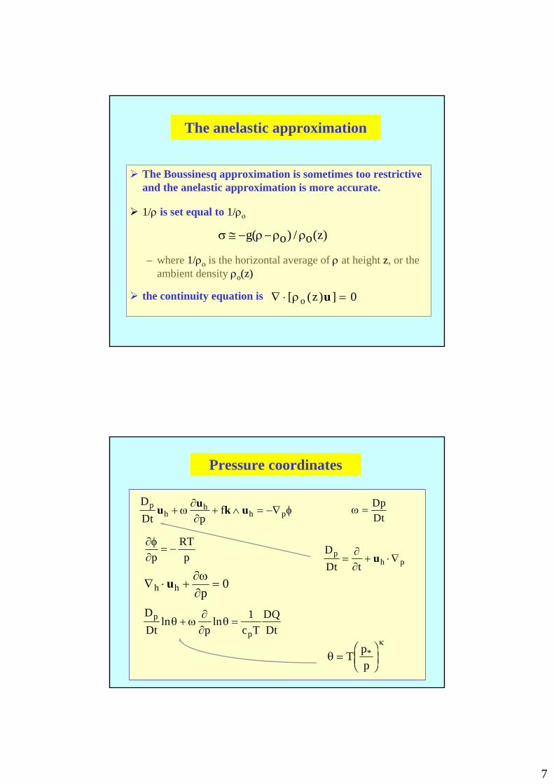
The anelastic approximation

The Boussinesq approximation is sometimes too restrictive and the anelastic approximation is more accurate.

1/ρ is set equal to 1/ρο

– where 1/ρο is the horizontal average of ρ at height z, or the ambient density ρo(z)

the continuity equation is

σ ρ ρ ρ≅ − −g o o z( ) / ( )

∇ ⋅ =[ ( ) ]ρo z u 0

Pressure coordinates

DDt p

fph

hh pu u k u+ + ∧ = −∇ω

∂∂

φ ω =DpDt

∂φ∂p

RTp

= −

∇ ⋅ + =h h pu ∂ω

∂0

DDt p c T

DQDt

p

pln lnθ ω

∂∂

θ+ =1

θκ

=FHGIKJT p

p*

DDt t

ph p= + ⋅ ∇

∂∂

u

8

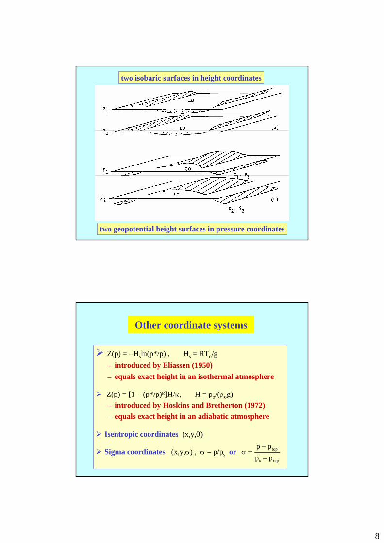
two isobaric surfaces in height coordinates

two geopotential height surfaces in pressure coordinates

Z(p) = −Hsln(p*/p) , Hs = RTo/g– introduced by Eliassen (1950)– equals exact height in an isothermal atmosphere

Z(p) = [1 − (p*/p)κ]H/κ, H = po/(ρog)– introduced by Hoskins and Bretherton (1972)– equals exact height in an adiabatic atmosphere

Isentropic coordinates (x,y,θ)

Sigma coordinates (x,y,σ) , σ = p/ps or

Other coordinate systems

top

s top

p pp p

−σ =

−

9

Plan

Start with the general equations

Linearize

Introduce tracers

Look for travelling wave solutions

Find the dispersion relation for such waves

Filter out sound waves

Filter out inertia-gravity waves

Chapter 2: Small-amplitude waves in a stably-stratified rotating atmosphere

Small-amplitude waves in a stably-stratified rotating atmosphere at rest

In a stably-stratified atmosphere at restdpdz

goo= − ρ

Equations for inviscid, isentropic motion:

DDt

f p gTu k u k+ ∧ = − ∇ −

1ρ

momentum

1 0ρ

ρDDt

+ ∇⋅ =u continuity

D sD t

= 0 specific entropy

p RT= ρ state

10

Some basics

s c cons t c cons tp p= + = +ln tan tanθ φ

φ θ= ln

N g ddz

g ddz

o

o

o2 = =φ

θθ N = Brunt-Väisälä frequency,

or buoyancy frequency

c RT po o o o2 = =γ γ ρ/ co = sound speed

1 1 1H

ddz

gRT T

dTdzs o

o

o o

o= − = +ρ

ρ Hs = density scale height

γ = c cp v/ ratio of specific heats

Note thatNg

gc Ho s

2

21

= − +

f = Coriolis parameter

Assumptions

two-dimensional perturbations

small-amplitude perturbations

∂∂

= ≠y

bu t v0 0,

| |u ⋅ ∇ < <∂∂ t

in DD t

11

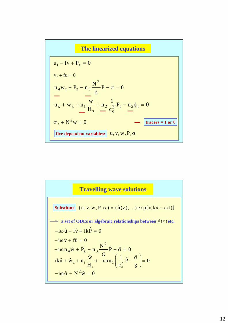
The linearized equations

u fv p zt o x− + =[ / ( )]ρ 0

v fut + = 0

n w p gt z o o4 0+ + =/ /ρ ρ ρ

u w n ddz

w nx zo

o t

o+ + + =1 2

1 0ρ

ρ ρρ

φ φt ozN+ =2 0

φγ

ρρ ρ

ρρ

= − = −pp

pco o o o o

2

tracers = 1 or 0

φρ

ρρ

= −pco o o

2

n w p gt z o o4 0+ + =/ /ρ ρ ρ

substitute

n w p pH

g pct o z

o s o o4 2

1 0+ − + −FHG

IKJ =( / )ρ

ρ ρφ

useNg

gc Ho s

2

21

= − + −Ng

p

o

2

ρ

insert tracer

n3

n w P n Ng

Pt z4 3

20+ − − =σ

P po

=ρ

o

g g′θ

σ = φ =θ

12

u fv Pt x− + = 0

v fut + = 0

u w n wH

nc

P nx zs o

t t+ + + − =1 2 2 21 0φ

σ t N w+ =2 0 tracers = 1 or 0

n w P n Ng

Pt z4 3

20+ − − =σ

five dependent variables: u v w P, , , , σ

The linearized equations

Travelling wave solutions

Substitute ( , , , , ) ( ( ), . . . ) exp[ ( )]u v w P u z i kx tσ ω= −

a set of ODEs or algebraic relationships between etc.( )u z

− − + =i u fv ikPω 0

− + =i v fuω 0

− + − − =i n w P n Ng

Pzω σ4 3

20

z 1 2 2s o

ˆ ˆw 1 ˆˆ ˆiku w n i n P 0H c g

⎛ ⎞σ+ + + − ω − =⎜ ⎟

⎝ ⎠− + =i N wωσ 2 0

13

L w A z P1 0( )+ =

B z w L P( ) + =2 0

u kf

P=−ω

ω 2 2 v ikff

P=−

−ω 2 2 σω

=Ni

w2

Three algebraic equations

Two ODEs

dwdz

Ng

n nH

w i kf

nc

Ps o

+ −LNM

OQP

+−

−LNM

OQP

=2

21

2

2 222 0ω

ω

ddz

Ng

n P i n N w−LNM

OQP

− −LNM

OQP

=2

3 4

2

2 0ωω

A single ODE

ddz

Ng

n kf

nc

ddz

Ng

n nH

w

n N w

o s−

LNM

OQP −

−FHG

IKJ + −FHG

IKJ

LNMM

OQPP

− − =

−2

3

2

2 222

1 2

21

24

2 0

ω

ω

If the boundary conditions are homogeneous, i.e. if at two horizontal boundaries, we have an eigenvalue problem for ω as a function of k.

w = 0

In general are functions of height, z.N c Ho s2 2, ,

In an isothermal atmosphere they are all constants.

14

First we consider waves in an unbounded region of fluidassuming that all terms are important, i.e., ni = 1 (i = 1,5).

Put sw(z) exp(imz z / 2H )∝ +

We obtain the dispersion relation for small amplitude waves:

ωω

4

02

2 2 22

2

02

2 2 2 22

14

14

0c

k mH

fc

N k f mHs s

− + + +FHG

IKJ + + +

FHG

IKJ =

Each of the perturbation quantities u, v, w, σ, P, varies inproportion to w ∝ exp[i(kx + mz – ωt + z/2Hs)]

or w i t z Hs∝ ⋅ − +exp[ ( ) / ]k x ω 2

Waves with all terms included

The wavelength is the distance in the direction of k over which k · x increases (or decreases) by 2π , i.e. λ = 2π/|k|

w i t z H s∝ ⋅ − +ex p[ ( ) / ]k x ω 2Consider

Here k = (k, m). It is not the unit vector in the vertical!

The planes k · x = constant are surfaces of constant phase

The wave 'crests' and 'troughs' are planes oriented normal to the vector k.

Note that the wave amplitude is appreciably uniform overheight ranges small compared with Hs, but increasesexponentially as z; this is related to the exponential decreaseof the density with height.

Plane waves

15

wavelength

crest

crest

crest

trough

trough

x

Wave crests and troughs in an unbounded plane wave

z

λ

k = (k, m)

1. Show that the phase speed of the plane wave is ω/|k| .

2. Show that the phase speed is not a vector; i.e., the components of the vector ω k /|k|2 are in general not equal to the components of the phase speed in the x and z directions.

Exercises

16

Dispersion relation in k - ω space

1. Geostrophic motion: ω = 0− = − = =fv p u and px o z o/ , , /ρ ρ σ0

Thus air parcels are displaced in the y-direction (v ≠ 0).

The solution holds whether or not N2, co2, and Hs are constant

and corresponds with a thermal wind in the y-direction

2. Inertia-gravity waves: ω2 2 2 2<< +( )k m co

Thenω2

2 2 2 2 2

2 2 2 2 21 4

1 4≈

+ ++ + +

N k f m Hk m H f c

s

s o

( / )/ /

This term is negligible

Possible wave modes

17

ω22 2 2 2 2

2 2 21 4

1 4≈

+ ++ +

N k f m Hk m H

s

s

( / )/

In the atmosphere at middle latitudes:

f ~ 10-4 s-1, N ~ 10-2 s-1, Hs ~ 104m and c0 ~ 103/3ms-1.

Then ε2 2 2 410 1= = <<−f N/

and ⇒ it can be neglected.

1 4 1 4 42 202 2 2

02 2/ / ( / ) /H f c H f c Hs s s+ = +Also

4 4 102 202 5H f cs / ≈ × −

Stratification and rotation are equally important when

N k f m Hs2 2 2 2 21 4≈ +( / )

If , this

Thus for λ << λo , rotation effects are negligible unless |m|is sufficiently large, implying a vertical wavelength muchless than Hs.

m Hs2 21 4<< /

in the atmosphere.

λ λ π≈ = ≈o sNH f km4 12000/

k f N Hs2 2 2 24≈ / )

ω22 2 2 2 2

2 2 21 4

1 4≈

+ ++ +

N k f m Hk m H

s

s

( / )/

18

~) /

wu

k(m + 1 / 4H2

s2 1 2 1>>

( / ) ( / )( / )P N g PN

m f Nz −= − =

+ −<<

2 2

2

2 2 21 1 4 1 1

σω H

k + m + 1 / 4Hs2

2 2s2

~ ( / )( ))

~/

/w i k mt

σω ω2 2 1 2

1 2 1+ −

− 1 / 4H

k (m + 1 / 4Hs2

2 2s2

k m Hs2 2 21 4>> + /

wavenumber vector

Particle motions in an internal gravity wave with

19

In this limit, ω → f.Then only Coriolis forces are important and the motion ispurely horizontal.Neither buoyancy nor pressure forces are significant.Such waves are called inertial waves.Pure inertial waves are regarded often as a meteorologicalcuriosity (Holton, pp59-60, §3.2.3).They may be important in atmospheric tidal motions, they are certainly observed in the oceans.In addition, since their phase speed cp = ω/k = f/k is large, they may be a computational nuisance.

3. Ultra-long waves: k → 0 ω 22 2 2 2 2

2 2 21 4

1 4≈

+ ++ +

N k f m Hk m H

s

s

( / )/

Nevertheless, inertial effects are observed in the atmosphere (see DM, Chapter 11).

When both rotation and stratification are important, though not necessarily comparable in magnitude, the waves are called inertia-gravity waves.

In the atmosphere, gravity waves usually have horizontalwavelengths 10 km and may be excited, for example, byairflow over orography, by convection penetrating astably-stratified air layer, or through shearing instability.

Inertial Effects

20

In this caseω2 2 2 2

021 4≈ + +( / )k m H cs

Consider the special case where mHs >> 1

( , ) ( , )u w k m P≈ −ω 1

the particle motions are in the direction of the wave, k, andare associated with negligible entropy change, φ ≈ 0.

These are well known properties of acoustic waves

• the waves are longitudinal, and

• the phase speed cp = ω/|k| ≈ co is large.

Mechanisms of excitation include lightening discharges andaeroplane noise (a rumble when clouds are around).

4. Acoustic waves: ω2 >> N2, f2

This does not lead to a trivial solution of the completesystem of equations, a nontrivial solution of which is

provided that

The equation

( )w z = 0

ω 2 2 202= +f k c

( )

12 2 22 1

3 22 2 2o s

2 24

d N k n d N n ˆn n wdz g f c dz g H

ˆn N w 0

−⎡ ⎤⎛ ⎞ ⎛ ⎞⎛ ⎞− − + −⎢ ⎥⎜ ⎟ ⎜ ⎟⎜ ⎟ ω −⎢ ⎥⎝ ⎠ ⎝ ⎠ ⎝ ⎠⎣ ⎦

− ω − =

has the trivial solution .( )w z = 0

5. Lamb waves: w = 0

21

− − + =i u fv ikPω 0 − + =i v fuω 0

unchanged

σ = 0

− + − − =i n w P n Ng

Pzω σ4 3

20

P n Ng

Pz − =3

20 ( ) ( ) /P z P eN z g= 0

2

iku w n wH

i nc

Pgz

s o+ + − −

FHG

IKJ =1 2 2

1 0ωσ

− + =i N wωσ 2 0

iku i n P c o/− =ω 22 0

( )w z = 0When

These solutions correspond to

( / ) ,u k P v and≈ ≈ =ω σ0 0

This solution is a so-called Lamb wave, modified slightly byrotation.

Its existence requires the ground (z = 0) to be flat, so that

( )w 0 0=

The pressure perturbation in the Lamb wave is essentiallysupported by the ground.

22

Example: water waves

z

h

z h x t= + ζ ( , )

pT = constant

D pD t

T = 0 at z h x t= + ζ ( , )

linearize∂∂

∂∂

ρpt

w d pd z

pt

gwoo+ = − = 0 at z = h

6. Boundary waves

∂∂

∂∂

ρpt

w d pd z

pt

gwoo+ = − = 0 at z = h

( / )P g i w= − ω

( , , , , ) ( ( ), . . . ) exp[ ( )]u v w P u z i kx tσ ω= −With

Usingddz

Ng

n P i n N w−LNM

OQP

− −LNM

OQP

=2

3 4

2

2 0ωω

set to 1

g d wd z

w− =ω 2 0 at z = h

23

The solution of

ddz

Ng

n kf

nc

ddz

Ng

n nH

w

n N w

o s−

LNM

OQP −

−FHG

IKJ + −FHG

IKJ

LNMM

OQPP

− − =

−2

3

2

2 222

1 2

21

24

2 0

ω

ω

g d wd z

w− =ω 2 0 at z = h

subject to

at z =0w = 0

is straightforward

no essential features are lost if we

- neglect the stratification; i.e., set N2 = 0 and omit theσ-equation, and

- assume the motion to be hydrostatic, wt << g; i.e., set n4 = 0(this assumption is valid provided that the waves are longenough), and

- assume there is no coupling between pressure and densityin the continuity equation ; i.e., set n2 = 0.

This suppresses acoustic waves

24

unchanged

− − + =i u fv ikPω 0 − + =i v fuω 0

− + − − =i n w P n Ng

Pzω σ4 3

20

iku w n wH

i nc

Pgz

s o+ + − −

FHG

IKJ =1 2 2

1 0ωσ

− + =i N wωσ 2 0 σ = 0

Pz = 0

Then

set n1 = 1

iku w wHz

s+ + = 0

Then ddz

Ng

n kf

nc

ddz

Ng

n nH

w

n N w

o s−

LNM

OQP −

−FHG

IKJ + −FHG

IKJ

LNMM

OQPP

− − =

−2

3

2

2 222

1 2

21

24

2 0

ω

ω

becomesd

dzd

dz Hw

s−

LNM

OQP

=1 0

g d wd z

w− =ω 2 0

Assume w = 0 at z = 0

at z = h

( ) [ e x p ( / ) ]w z W z H s= −1

where W is a constant

25

1. are related to W, ,u v P

2. Pz = 0

Notes:

tanP cons t=

3. If satisfies( ) [ e x p ( / ) ]w z W z H s= −1

g d wd z

w− =ω 2 0 at z = h

then

ω 2 2 2 1= + − −f g H k h Hs s[ e x p ( / ) ]

The solution corresponds to a free surface wave

The effects of shear

see later

acoustic waves are refracted by superimposed shear; enhanced downwind audibility results from the convergent refraction of sound waves, usually due to wind shear, but, occasionally, temperature variations may play a role also.

gravity waves may be severely modified by shear. The refraction effect is considerable and leads to the totalreflection of some (shorter) components which may betrapped in channels as well-marked trains of lee waves downstream of mountains. In certain situations waves may be absorbed also.

where vorticity gradients are large, gravity waves may growspontaneously by Kelvin-Helmholtz instability, giving rise tobillows or clear air turbulence (CAT).

26

12

2 24

23

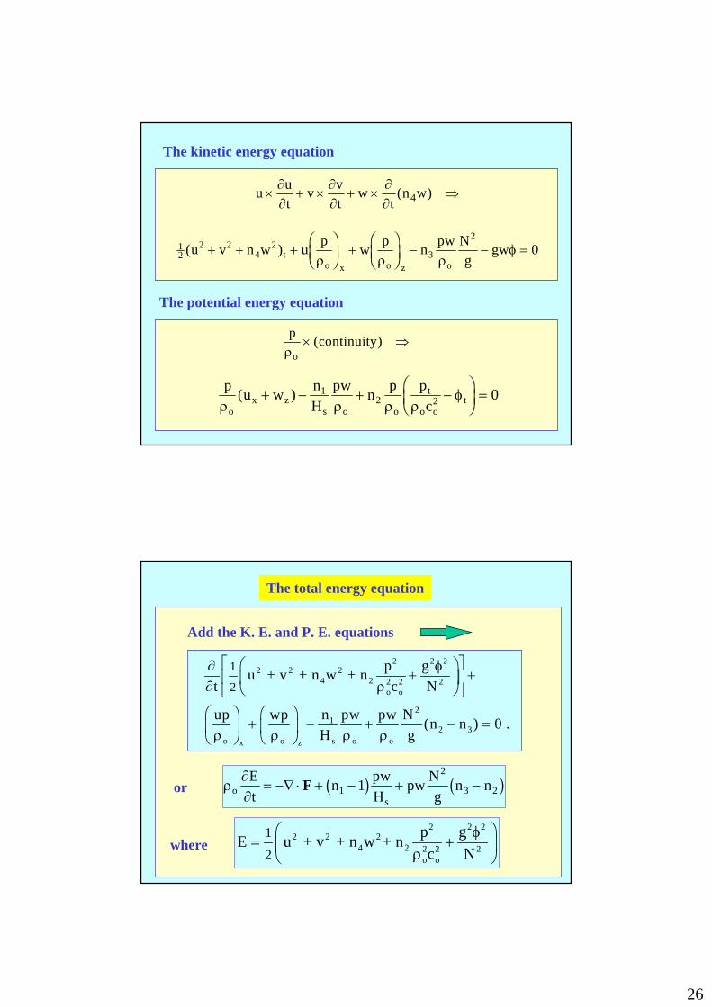
20( )u v n w u p w p n pw N

ggwt

o x o z o+ + +

FHGIKJ +FHGIKJ − − =

ρ ρ ρφ

The kinetic energy equation

The potential energy equation

u ut

v vt

wt

n w× + × + × ⇒∂∂

∂∂

∂∂

( )4

p continuityoρ

× ⇒( )

p u w nH

pw n p pco

x zs o o

t

o otρ ρ ρ ρ

φ( )+ − + −FHG

IKJ =1

2 2 0

2 2 22 2 2

4 2 2 2 2o o

21

2 3o o s o ox z

1

2

p gu + v + n w + nt c N

up wp n pw pw N (n n ) 0 .H g

⎡ ⎤⎛ ⎞∂ φ+ +⎢ ⎥⎜ ⎟∂ ρ⎝ ⎠⎣ ⎦

⎛ ⎞ ⎛ ⎞+ − + − =⎜ ⎟ ⎜ ⎟ρ ρ ρ ρ⎝ ⎠ ⎝ ⎠

or ρ∂∂o

s

Et

n pwH

pw Ng

n n= −∇ ⋅ + − + −F 1

2

3 21b g b g

where2 2 2

2 2 24 2 2 2 2

o o

1

2

p gE u + v + n w + nc N

⎛ ⎞φ= +⎜ ⎟ρ⎝ ⎠

Add the K. E. and P. E. equations

The total energy equation

27

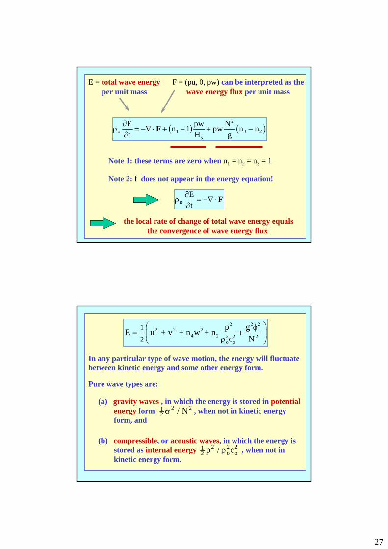
E = total wave energyper unit mass

F = (pu, 0, pw) can be interpreted as thewave energy flux per unit mass

ρ∂∂o

s

Et

n pwH

pw Ng

n n= −∇ ⋅ + − + −F 1

2

3 21b g b g

Note 2: f does not appear in the energy equation!

Note 1: these terms are zero when n1 = n2 = n3 = 1

ρ∂∂oEt

= −∇ ⋅ F

the local rate of change of total wave energy equalsthe convergence of wave energy flux

In any particular type of wave motion, the energy will fluctuatebetween kinetic energy and some other energy form.

Pure wave types are:

(a) gravity waves , in which the energy is stored in potentialenergy form , when not in kinetic energyform, and

12

2 2σ / N

(b) compressible, or acoustic waves, in which the energy isstored as internal energy , when not inkinetic energy form.

12

2 2 2p co o/ ρ

2 2 22 2 2

4 2 2 2 2o o

1

2

p gE u + v + n w + nc N

⎛ ⎞φ= +⎜ ⎟ρ⎝ ⎠

28

12

2 2σ / N12

2 2 2p co o/ ρ

Inertia-gravity waves undergo energy conversions similar to pure gravity waves.

In general, waves of the mixed gravity-acoustic type are such that kinetic energy is converted partly into potential energy and partly into internal energy.

However, in this case, the interpretations of aspotential energy and as internal energy are notstrictly correct.

If the tracers ni are retained and the expression

is substituted into

( ) exp /w z im n H zs∝ + 1 2b g

ddz

Ng

n kf

nc

ddz

Ng

n nH

w

n N w

s−

FHG

IKJ −

−FHG

IKJ + −FHG

IKJ

LNMM

OQPP

− − =

−2

3

2

2 22

02

1 2

21

24

2 0

ω

ω( )

we obtain

Simplified solutions and filtered equations

29

The consequences of omitting certain terms in the equations ofmotion may now be investigated.

It is desirable that any approximation yields a consistent energy equation.

m nH

Ng

im n n n n Ng H

n n n n

n N kf

n nc

s s

o

2 12

2

2

3 2 2 3

2

212 1 2 3

42 2

2

2 2 2 4

2

2

41 1

0

+ + − + − + − +LNM

OQP

+ −−

− =

( ) ( ) ( )

( ) .

l q

ωω

ω

Examination of

suggests that setting n2 = 0 in

will remove the acoustic mode from the equations.

u w n wH

nc

p nx zs o o t

t+ − +LNMOQP

− =122 2 0

ρφ

'Sound-proofing' the equations

2 2 22 2 2

4 2 2 2 2o o

21

2 3o o s o ox z

1

2

p gu + v + n w + nt c N

up wp n pw pw N (n n ) 0 .H g

⎡ ⎤⎛ ⎞∂ φ+ +⎢ ⎥⎜ ⎟∂ ρ⎝ ⎠⎣ ⎦

⎛ ⎞ ⎛ ⎞+ − + − =⎜ ⎟ ⎜ ⎟ρ ρ ρ ρ⎝ ⎠ ⎝ ⎠

30

The equation

then gives

m nH

Ng

im n n n n Ng H

n n n n

n N kf

n nc

s s

o

2 12

2

2

3 2 2 3

2

212 1 2 3

42 2

2

2 2 2 4

2

2

41 1

0

+ + − + − + − +LNM

OQP

+ −−

− =

( ) ( ) ( )

( ) .

l q

ωω

ω

ω2

2 2 2 24 3 2

42 2

4 3 2

12

22 1

12

22 1

=+ + + −FH IK

+ + + −

N k f m n im

n k m n im

nH

Ng

nH

nH

Ng

nH

s s

s s

e je j

When n1 = n4 = 1, this differs from the dispersion relation forinertia-gravity waves only in respect of the terms involving n3.

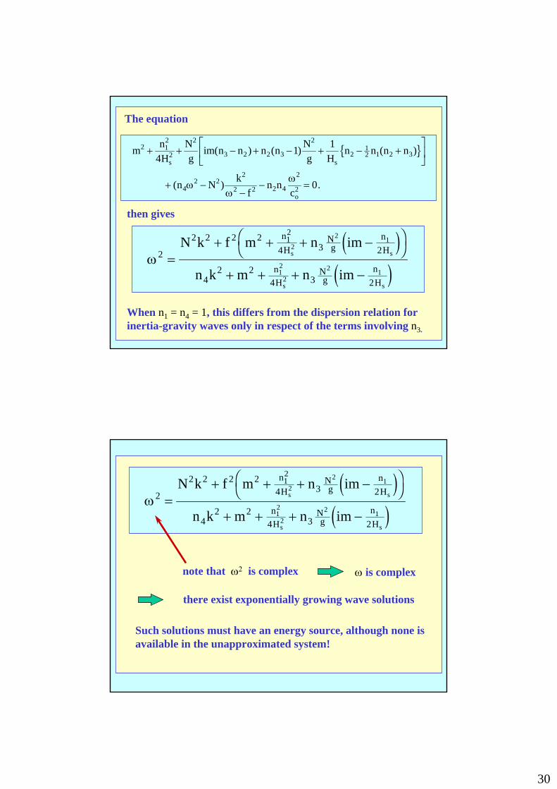
ω2

2 2 2 24 3 2

42 2

4 3 2

12

22 1

12

22 1

=+ + + −FH IK

+ + + −

N k f m n im

n k m n im

nH

Ng

nH

nH

Ng

nH

s s

s s

e je j

note that ω2 is complex ω is complex

there exist exponentially growing wave solutions

Such solutions must have an energy source, although none isavailable in the unapproximated system!

31

The equation

ρ∂∂o

s

Et

n pwH

pw Ng

n n= −∇ ⋅ + − + −F 1

2

3 21b g b g

shows that with n2 = 0, there is an energy source unless n3 = 0.

Hence, to filter sound waves from the system of equations,we must take both n2 and n3 to be zero to preserve energeticconsistency.

Note that sound waves are filtered out also by letting co2 → ∞

Filtering the sound waves

In many atmospheric situations, the pressure is very close toits hydrostatic value.

In the foregoing analysis, pressure is hydrostatic if n4 = 0.

This eliminates Dw/Dt, or in linearized form ∂w/∂t , from thevertical momentum equation.

With n1 = n2 = n3 = 1, the dispersion relation gives

− + + + +FHG

IKJ − − +

FHG

IKJ =n

cm

Hn f

cn k N k f m

Ho s o s4

4

22 2

2 4

2

2 42 2 2 2 2

21

41

40ω

ω

The hydrostatic approximation

32

The terms involving n4 are negligible if

ω2

22

21

4cm

Ho s<< +(a)

(b) ω2 2<< N

− + + + +FHG

IKJ − − +

FHG

IKJ =n

cm

Hn f

cn k N k f m

Ho s o s4

4

22 2

2 4

2

2 42 2 2 2 2

21

41

40ω

ω

typically well satisfied forinertia-gravity waves

More discriminating

If a layer is close to adiabatic, then , and the dispersionrelation becomes

N 2 0≈

ω 2 22 4

2 2 22

14

14

mH

n k f mHs s

+ +FHG

IKJ = +FHG

IKJ k m2 2<<

Since for finite N2

ω 2 2 2 2 22 4

2 22

14

14

= + +FHG

IKJ

LNM

OQP

+ +FHG

IKJN k f m

Hn k m

Hs s/

The condition k2 << m2 implies that ω2 << N2

The hydrostatic approximation may be considered appropriatewhenever k2 << m2 is satisfied.

The hydrostatic approximation is valid for waves whosehorizontal wavelength is much larger than the vertical wavelength.

33

Note that the magnitude of g-1Dw/Dt is irrelevant to the usefulness of the hydrostatic approximation for finding the acceleration.

Even if this quantity is small, the dynamics will be incorrectlymodelled by its neglect if the motion is in tall narrow columns,i.e. if m2 << k2 .

The condition k2 << m2 is usually well satisfied for large-scaleatmospheric motions and the hydrostatic approximation is used exclusively in 'primitive equation' (PE) numerical weather prediction (NWP) models.

If we formally set n1 = 1 and n2 = n3 = n4 = 0, valid under thesame conditions (a) and (b) for the hydrostatic approximationalone, the dispersion relation gives

The Lamb wave now disappears as it does when the other acoustic waves are eliminated. However, the free surface wave still exists and leads to a spurious fast moving wave. It is filtered out by using a rigid-lid condition. A primitive equation, numerical weather prediction model can be devised for the set of equations with n1 = 1 and n2 = n3 = n4 = 0 together with a rigid upper boundary condition.

ω 2 2 2 2 2 21 4= + +f N k m Hs/ ( / )

Sound-proofed hydrostatic approximation

34

Variation of mean density with height; the equivalent incompressible atmosphere

The upward decrease of mean density that distinguishes betweencontinuity of volume and mass is represented by the term in n1and appears in the multiplier in etc. exp( / )z H s o2 ∝ ρ wOver tropospheric depths this factor is significant, but elsewheren1 appears only in the combination m2 + n1/4Hs

2 and then it is often negligible, e.g. if 2 2 21

s s 4m / H , 1/ 4H (m / ) m / 40= π = π ≈

When the vertical length scale of the motion is not large, thedensity variation can be neglected by setting n1 = 0 as long as thefactor is included implicitly.ρo

A prediction of u obtained from the incompressible (Boussinesq)model should then be compared with observed inthe (compressible) atmosphere, where .

( / )ρ ρo s uρ ρs o= ( )0

The solution of

corresponding with ω = 0 is independent of the values ofn1 − n4, but the more general "quasi-geostrophic" solutionsare not.

ωω

4

02

2 2 22

2

02

2 2 2 22

14

14

0c

k mH

fc

N k f mHs s

− + + +FHG

IKJ + + +

FHG

IKJ =

If we are interested only in the slowly-moving, nearly geostrophic waves, we can omit sound waves and suppose that the pressure is hydrostatic, i.e., put n2 = n3 = n4 = 0.

Geostrophic motion

35

The Boussinesq equations for a non-rotating stratified liquid are:

DDt

pu= − ∇ +

1ρ

σ*

k ∇ ⋅ =u 0 DDt

ρ= 0

Show that the dispersion relation for small-amplitude wavesin the x-z plane is

ω22 2

2 2=+

N kk m

Exercise (2.10)

The End