Admin. Recap: Routing - Zoo | Yale...

Network Layer: Non-Traditional Wireless Routing

Localization Intro

Y. Richard Yang

12/4/2012

2

Outline

❒ Admin. and recap ❒ Network layer

❍  Intro ❍  Location/service discovery ❍ Routing

•  Traditional routing •  Non-traditional routing

❒  Localization ❍  Intro

Admin. ❒  Projects

❍  please use Sign Up on classesv2 for project meetings

❍  project code/<6-page report due Dec. 12 ❍  final presentation date? ❍ First finish a basic version, and then stress/

extend your design

3 4

Recap: Routing

❒ So far, all routing protocols are in the framework of traditional wireline routing ❍  a graph representation of underlying network

•  point-to-point graph, edges with costs ❍  select a best (lowest-cost) route for a src-dst

pair

5

Traditional Routing

❒ Q: which route?

6

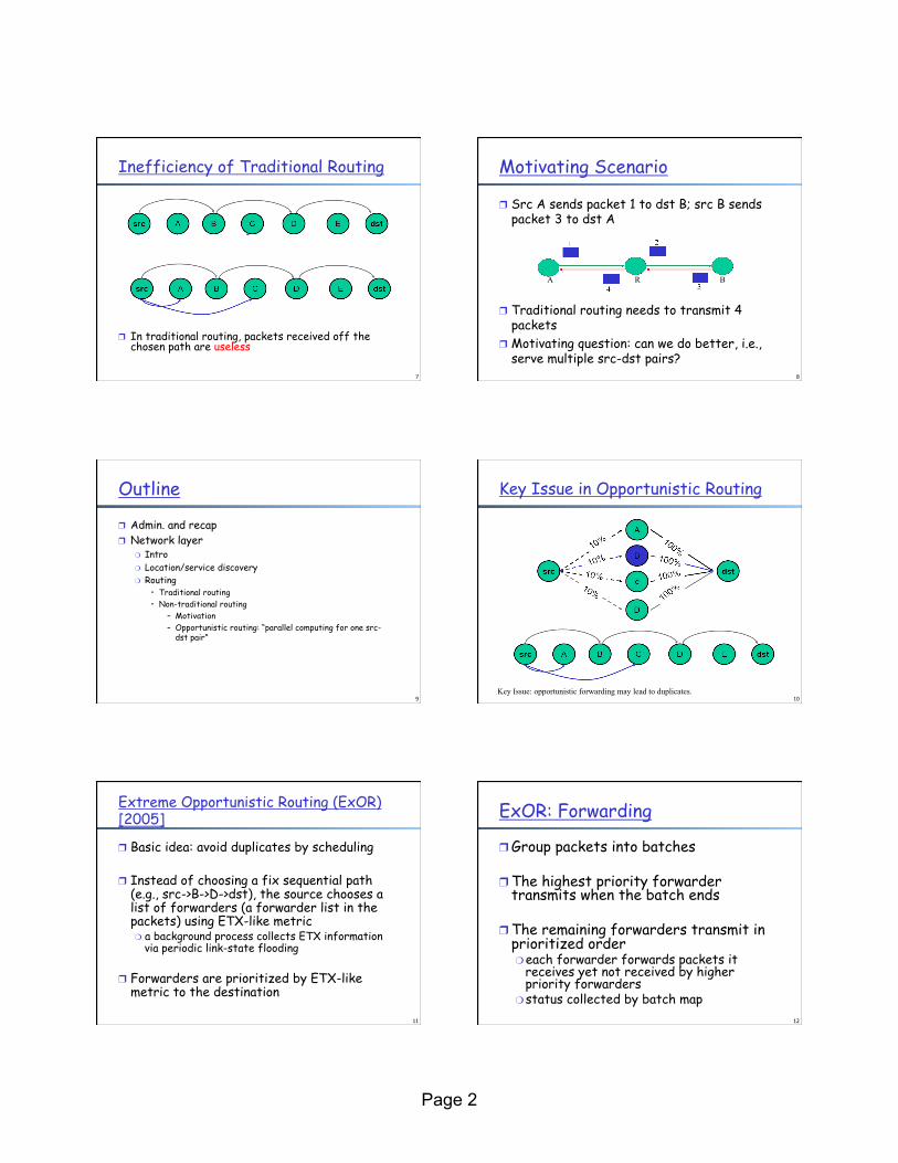
Inefficiency of Traditional Routing

❒  In traditional routing, packets received off the chosen path are useless

❒  Q: what is the probability that at least one of the intermediate nodes will receive from src?

7

Inefficiency of Traditional Routing

❒  In traditional routing, packets received off the chosen path are useless

8

Motivating Scenario

❒ Src A sends packet 1 to dst B; src B sends packet 3 to dst A

❒ Traditional routing needs to transmit 4 packets

❒ Motivating question: can we do better, i.e., serve multiple src-dst pairs?

A B R

9

Outline

❒  Admin. and recap ❒  Network layer

❍  Intro ❍  Location/service discovery ❍  Routing


–  Motivation –  Opportunistic routing: “parallel computing for one src-

dst pair”

Key Issue in Opportunistic Routing

10 Key Issue: opportunistic forwarding may lead to duplicates.

11

Extreme Opportunistic Routing (ExOR) [2005]

❒  Basic idea: avoid duplicates by scheduling

❒  Instead of choosing a fix sequential path (e.g., src->B->D->dst), the source chooses a list of forwarders (a forwarder list in the packets) using ETX-like metric ❍  a background process collects ETX information

via periodic link-state flooding

❒  Forwarders are prioritized by ETX-like metric to the destination

12

ExOR: Forwarding

❒ Group packets into batches

❒ The highest priority forwarder transmits when the batch ends

❒ The remaining forwarders transmit in prioritized order ❍ each forwarder forwards packets it

receives yet not received by higher priority forwarders

❍ status collected by batch map

13

Batch Map

❒  Batch map indicates, for each packet in a batch, the highest-priority node known to have received a copy of that packet

ExOR: Example

14

N0

N3

N1

N2

ExOR: Stopping Rule

❒ A nodes stops sending the remaining packets in the batch if its batch map indicates over 90% of this batch has been received by higher priority nodes ❍ the remaining packets transferred with

traditional routing

15 16

Evaluations

❒  65 Node pairs ❒  1.0MByte file

transfer ❒  1 Mbit/s 802.11 bit

rate ❒  1 KByte packets ❒  EXOR bacth size

100

1 kilometer

17

Evaluation: 2x Overall Improvement

❒  Median throughputs: 240 Kbits/sec for ExOR, 121 Kbits/sec for Traditional

Throughput (Kbits/sec)

1.0

0.8

0.6

0.4

0.2

0 0 200 400 600 800

Cum

ulat

ive

Frac

tion

of N

ode

Pai

rs

ExOR Traditional

18

OR uses links in parallel

Traditional Routing 3 forwarders

4 links

ExOR 7 forwarders

18 links

19

OR moves packets farther

❒  ExOR average: 422 meters/transmission ❒  Traditional Routing average: 205 meters/tx

Frac

tion

of T

rans

mis

sion

s

0

0.1

0.2

0.6 ExOR Traditional Routing

0 100 200 300 400 500 600 700 800 900 1000

Distance (meters)

25% of ExOR transmissions

58% of Traditional Routing transmissions

20

Comments: ExOR

❒  Pros ❍  takes advantage of link diversity (the

probabilistic reception) to increase the throughput

❍  does not require changes in the MAC layer ❍  can cope well with unreliable wireless medium

❒  Cons ❍  scheduling is hard to scale in large networks ❍  overhead in packet header (batch info) ❍  batches increase delay

21

Outline





dst pair” » ExOR » MORE

MORE: MAC-independent Opportunistic Routing & Encoding [2007]

❒  Basic idea: ❍ Replace node coordination with network coding ❍ Trading structured scheduler for random

packets combination

22

Basic Idea: Source

❒  Chooses a list of forwarders (e.g., using ETX)

❒  Breaks up file into K packets (p1, p2, …, pK) ❒ Generate random packets

❒ MORE header includes the code vector

[cj1, cj2, …cjK] for coded packet pj’

23

∑= ijij pcp '

Basic Idea: Source

24

Basic Idea: Forwarder

❒  Check if in the list of forwarders ❒  Check if linearly independent of new packet

with existing packet ❒  Re-coding and forward

25

Basic Idea: Destination

❒ Decode

❒ Send ACK back to src if success

26

Key Practical Question: How many packets does a forwarder send?

❒  Compute zi: the expected number of times that forwarder i should forward each packet

27

Computes zs

28

)1(1

sjj

sz ε∏−=Compute zs so that at least one forwarder that is closer to destination is expected to have received the packet :

Єij: loss probability of the link between i and j

Compute zj for forwarder j

❒ Only need to forward packets that are ❍  received by j ❍  sent by forwarders who are further from

destination ❍  not received by any forwarder who is closer to

destination

❒ #such pkts:

29

])1([zfurther is d closer to

i iki k

ijjL εε∑ ∏−=

Compute zj for forwarder j

❒ To guarantee at least one forwarder closer

to d receives the packet

30

])1([zfurther is d closer to

i iki k

ijjL εε∑ ∏−=

)1(d closer to jk

k

jLjz ε∏−=

Evaluations

❒  20 nodes distributed in a indoor building ❒  Path between nodes are 1 ~ 5 hops in length ❒  Loss rate is 0% ~ 60%; average 27%

31

Throughput

32

Improve on MORE?

33

Mesh Networks API So Far

Network

Forward correct packets to destination

PHY/LL Deliver correct packets

S

R1

R2

D

10-3 BER

10-3 BER

Motivation

0%

0%

570 bytes; 1 bit in 1000 incorrect à Packet loss of 99%

S

R1

R2

D

99% (10-3 BER)

99% (10-3 BER)

Implication

0%

0%

Opportunis?c Rou?ng à 50 transmissions

Loss

Loss

ExOR MORE

37

Outline





dst pair” » ExOR [2005] » MORE [2007] » MIXIT [2008]

New API

PHY + LL

Deliver correct symbols to higher layer

Network Forward correct symbols to destination

What Should Each Router Forward?

R1

R2

D S P1 P2

P1 P2

P1 P2

What Should Each Router Forward?

R1

R2

D S P1 P2

1)  Forward everything à Inefficient 2) Coordinate à Unscalable

P1 P2

P1 P2

P1 P2

P1 P2

Forward random combinations of correct symbols

R1

R2

D S P1 P2

Symbol Level Network Coding

P1 P2

P1 P2

1s

…

… R1

R2

D

2s2

1

7s2s+

2

7

…

1s

…

…

2s

Routers create random combinations of correct symbols

2

1

9s5s+

5

9

…


R1

R2

D 2

1

7s2s+

…

2

1

9s5s+

…

21 s,sSolve 2

equa?ons

Destination decodes by solving linear equations


1s

…

… R1

R2

D

2s2

1

7s2s+

2

7

…

1s

…

…

2s

Routers create random combinations of correct symbols

15s5

0

…


R1

R2

D 2

1

7s2s+

…

15s …

21 s,sSolve 2

equa?ons

Destination decodes by solving linear equations

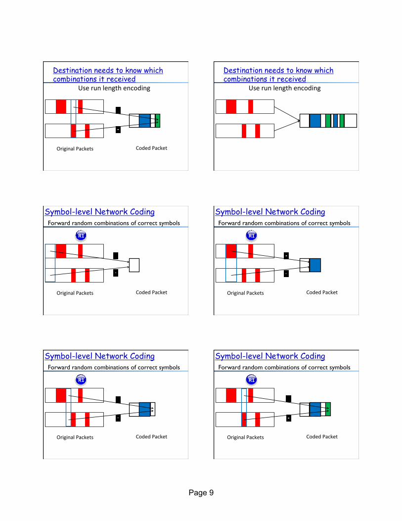
Symbol Level Network Coding Destination needs to know which combinations it received

Use run length encoding 5

9

Original Packets Coded Packet

5

9

0

9


Use run length encoding

Destination needs to know which combinations it received

9

5




0

5






Symbol-level Network Coding

5

9


R1


0

9



R1


9

5



R1


0

5



R1


Evaluation

•  Implementa9on on GNURadio SDR and USRP •  Zigbee (IEEE 802.15.4) link layer •  25 node indoor testbed, random flows •  Compared to:

1.  Shortest path rou9ng based on ETX 2.  MORE: Packet-‐level opportunis9c rou9ng

0

0.2

0.4

0.6

0.8

1

0 20 40 60 80 100 Throughput (Kbps)

CD

F

Throughput Comparison

2.1x

3x

Shortest Path MORE MIXIT

57

Outline





dst pair” –  Opportunistic routing: “parallel computing for

multiple src-dst pairs”

58

Motivating Scenario

❒ A sends pkt 1 to dst B ❒  B sends pkt 3 to dst A

A B R

Opportunistic Coding: Basic Idea

❒  Each node looks at the packets available in its buffer, and those its neighbors’ buffers

❒  It selects a set of packets, computes the XOR of the selected packets, and broadcasts the XOR

59 60

Opportunistic Coding: Example

61

Wireless Networking: Summary

send receive

status

info info/control

-  The ability to communicate is a foundational support of wireless mobile networks - The capacity of such networks is continuously being challenged as demand increases (e.g., Verizon LTE-based home broadband) -  Much progress has been made, but still more are coming.

Outline

❒ Admin. ❒ Network layer ❒  Localization

❍  overview

62

63

Motivations ❒ The ancient question:

Where am I?

❒  Localization is the process of determining the positions of the network nodes

❒ This is as fundamental a primitive as the ability to communicate

64

Localization: Many Applications

❒  Location aware information services ❍  e.g., E911, location-based search,

advertisement, inventory management, traffic monitoring, emergency crew coordination, intrusion detection, air/water quality monitoring, environmental studies, biodiversity, military applications, resource selection (server, printer, etc.)

❒  “Sensing data without knowing the location is meaningless.” [IEEE Computer, Vol. 33, 2000]

65

Measurements

The Localization Process

Localizability (opt)

Location Computation

Location Based Applications

66

Classification of Localization based on Measurement Modality ❒  Coarse-grained measurements, e.g.,

❍  signal signature •  a database of signal signature (e.g. pattern of received signal,

visible set of APs (http://www.wigle.net/)) at different locations

•  match to the signature ❍  Connectivity

❒  Advantages ❍  low cost; measurements do not need line-of-sight

❒  Disadvantages ❍  low precision

For a detailed study, see “Accuracy Characterization for Metropolitan-scale Wi-Fi Localization,” in Mobisys 2005.

67

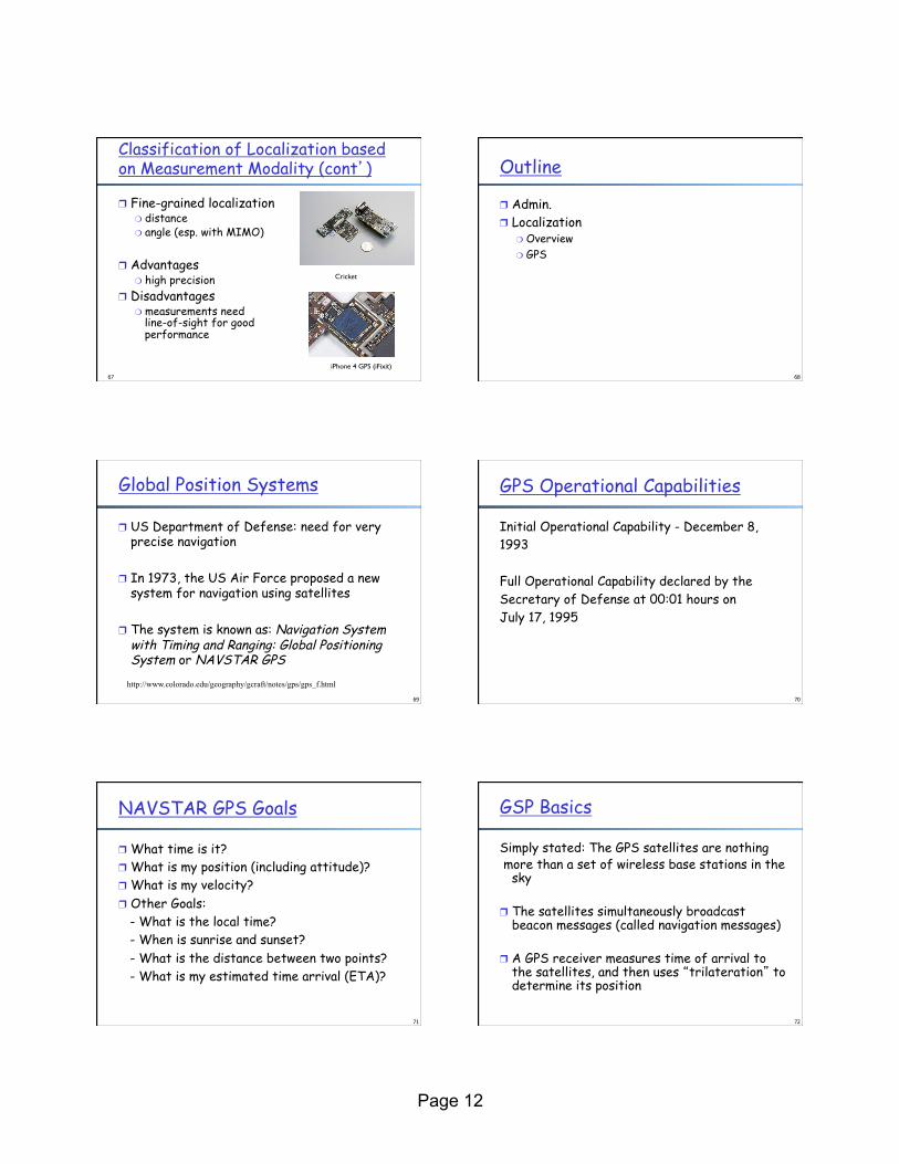
Classification of Localization based on Measurement Modality (cont’)

❒  Fine-grained localization ❍  distance ❍  angle (esp. with MIMO)

❒ Advantages ❍  high precision

❒ Disadvantages ❍ measurements need

line-of-sight for good performance

Cricket

iPhone 4 GPS (iFixit)

Outline

❒ Admin. ❒  Localization

❍ Overview ❍ GPS

68

69

Global Position Systems

❒ US Department of Defense: need for very precise navigation

❒  In 1973, the US Air Force proposed a new system for navigation using satellites

❒ The system is known as: Navigation System with Timing and Ranging: Global Positioning System or NAVSTAR GPS

http://www.colorado.edu/geography/gcraft/notes/gps/gps_f.html

70

GPS Operational Capabilities

Initial Operational Capability - December 8, 1993 Full Operational Capability declared by the Secretary of Defense at 00:01 hours on July 17, 1995

71

NAVSTAR GPS Goals

❒ What time is it? ❒ What is my position (including attitude)? ❒ What is my velocity? ❒ Other Goals: - What is the local time? - When is sunrise and sunset? - What is the distance between two points? - What is my estimated time arrival (ETA)?

72

GSP Basics

Simply stated: The GPS satellites are nothing more than a set of wireless base stations in the

sky ❒ The satellites simultaneously broadcast

beacon messages (called navigation messages)

❒ A GPS receiver measures time of arrival to the satellites, and then uses “trilateration” to determine its position

73

GPS Basics: Triangulation

❒ Measurement:

Computes distance cpp

tt SR 11 −+=

)( 11

SR ttcpp −=−

74

GPS Basics: Triangulation

❒  In reality, receiver clock is not sync’d with satellites

❒ Thus need to estimate clock

driftclockSR

cdtt −++= δ11 )( 1

1 driftclockSR ttcpp −−−=− δ

driftclockSR cttc −−−= δ)( 1

called pseudo range

75

GPS with Clock Synchronization?

76

GPS Design/Operation

❒ Segments (components) ❍ user segment: users with receivers

❍ control segment: control the satellites

❍ space segment: •  the constellation of satellites •  transmission scheme

77

Control Segment Master Control Station is located at the Consolidated Space Operations Center (CSOC) at Flacon Air Force Station near Colorado Springs

78

CSOC

❒ Track the satellites for orbit and clock determination

❒ Time synchronization

❒ Upload the Navigation Message

❒ Manage Denial Of Availability (DOA)

79

Space Segment: Constellation

80

Space Segment: Constellation

❒ System consists of 24 satellites in the operational mode: 21 in use and 3 spares

3 other satellites are used for testing ❒ Altitude: 20,200 Km with periods of 12 hr. ❒  Current Satellites: Block IIR-

$25,000,000 2000 KG ❒ Hydrogen maser atomic clocks

❍  these clocks lose one second every 2,739,000 million years

81

GPS Orbits

82

GPS Satellite Transmission Scheme: Navigation Message ❒  To compute position one must know the positions

of the satellites

❒  Navigation message consists of: - satellite status to allow calculating pos - clock info

❒  Navigation Message at 50 bps ❍  each frame is 1500 bits ❍  Q: how long for each message?

More detail: see http://home.tiscali.nl/~samsvl/nav2eu.htm

83

GPS Satellite Transmission Scheme: Requirements

❒ All 24 GPS satellites transmit Navigation Messages on the same frequencies

❒  Resistant to jamming

❒  Resistant to spoofing

❒ Allows military control of access (selected availability)

84

GPS As a Communication Infrastructure

❒ All 24 GPS satellites transmit on the same frequencies BUT use different codes ❍  i.e., Direct Sequence Spread Spectrum (DSSS),

and ❍  Code Division Multiple Access (CDMA) ❍ Using BPSK to encode bits

85

Basic Scheme

86

GPS Control

❒  Controlling precision ❍  Lower chipping rate, lower precision

❒  Control access/anti-spoofing ❍  Control chipping sequence

87

GPS Chipping Seq. and Codes

❒ Two types of codes ❍  C/A Code - Coarse/Acquisition Code available

for civilian use on L1 •  Chipping rate: 1.023 M •  1023 bits pseudorandom numbers (PRN)

❍  P Code - Precise Code on L1 and L2 used by the military

•  Chipping rate: 10.23 M •  PRN code is 6.1871 × 1012 (repeat about one week) •  P code is encrypted called P(Y) code

http://www.navcen.uscg.gov/gps/geninfo/IS-GPS-200D.pdf

http://www.gmat.unsw.edu.au/snap/gps/gps_survey/chap3/chap3.htm 88

GPS PHY and MAC Layers

89

Typical GPS Receiver: C/A code on L1

❒ During the “acquisition” time you are receiving the navigation message also on L1

❒ The receiver then reads the timing information and computes “pseudo-ranges”

Military Receiver

❒ Decodes both L1 and L2 ❍  L2 is more precise ❍  L1 and L2

difference allows computing ionospheric delay

90

91

Denial of Accuracy (DOA)

❒ The US military uses two approaches to prohibit use of the full resolution of the system

❒ Selective availability (SA) ❍  noise is added to the clock signal and ❍  the navigation message has “lies” in it ❍ SA is turned off permanently in 2000

❒ Anti-Spoofing (AS) - P-code is encrypted

92

Extensions to GPS ❒  Differential GPS

❍  ground stations with known positions calculate positions using GPS ❍  the difference (fix) transmitted using FM radio ❍  used to improve accuracy

❒  Assisted GPS ❍  put a server on the ground to help a GPS receiver ❍  reduces GPS search time from minutes to seconds ❍  E.g., iPhone GPS:

http://www.broadcom.com/products/GPS/GPS-Silicon-Solutions/BCM4750

93

GPS: Summary

❒ GPS is among the “simplest” localization technique (in terms topology): one-step trilateration

94

GPS Limitations

❒ Hardware requirements vs. small devices

❒ GPS can be jammed by sophisticated adversaries

❒ Obstructions to GPS satellites common •  each node needs LOS to 4 satellites •  GPS satellites not necessarily overhead, e.g., urban

canyon, indoors, and underground

95

Percentage of localizable nodes localized by Trilateration.

Uniformly random 250 node network.

Limitation of Trilateration

Rat

io

Average Degree

Admin. Recap: Routing - Zoo | Yale...

Documents

Transcript of Admin. Recap: Routing - Zoo | Yale...