Adjusting Numerical Model Data in Real Time: AQMOS Prepared by Clinton P. MacDonald, Dianne S....
15
Adjusting Numerical Model Data in Real Time: AQMOS Prepared by Clinton P. MacDonald, Dianne S. Miller, Timothy S. Dye, Kenneth J. Craig, Daniel M. Alrick Sonoma Technology, Inc. Petaluma, CA Presented at the 2010 National Air Quality Conferences Raleigh, NC March 15-18, 2010 3805
-
Upload
tyler-townsend -
Category
Documents
-
view
215 -
download
2
Transcript of Adjusting Numerical Model Data in Real Time: AQMOS Prepared by Clinton P. MacDonald, Dianne S....

Adjusting Numerical Model Data in Real Time: AQMOS
Prepared byClinton P. MacDonald, Dianne S. Miller, Timothy S. Dye,
Kenneth J. Craig, Daniel M. AlrickSonoma Technology, Inc.
Petaluma, CA
Presented at the 2010 National Air Quality ConferencesRaleigh, NC
March 15-18, 2010
3805

2
Introduction
What: The Air Quality Model Output Statistics (AQMOS) forecasting tool provides air quality model predictions adjusted in real time.
Why: Gridded numerical weather and air quality models have some errors in their predictions.
How: Like model output statistics for weather models, AQMOS uses regression equations to correct for air quality model errors.
AQMOS is• Automated• Dynamically updated after each
model run• City-, pollutant-, and model-specific

3
How AQMOS Works
• AQMOS calculates regression equations from recent air quality observations and numerical model predictions (the critical component).
• The forecasting tool applies these equations to the current numerical model predictions.
AQMOS prediction = numerical model prediction x correlation factor + constant
+
0
5
10
15
20
25
30
35
0 10 20 30 40 50
Model predicted PM2.5 (ug/m3)
Ob
se
rve
d P
M2
.5 (
ug
/m3
)
Many days of observed and predicted data

4
AQMOS Data Sources
• Air quality observations from AIRNow Gateway – Peak daily 8-hr ozone– Daily 24-hr PM2.5
• Model data– NOAA Air Quality Forecast Guidance (6Z and 12Z)– BlueSky Gateway Experimental CMAQ (0Z)
The system’s flexibility allows new models and parameters to be added as data become available.

5
Acquire Data
Extract the concentration at the geographic centroid of each ZIP Code and calculate the maximum concentration in the area (in this example, 53 ppb for Des Moines).
Hourly NOAA grib data provides peak next-day 8-hr ozone forecast.
Store daily predictions for each area and model run in AQMOS database.
AQMOSAIRNow Gateway files provide peak 8-hr ozone concentrations for each forecast area.
AIRNowGatewayData File
Store daily peak concentration data in AQMOS database.

6
Calculate Regression
• Match recent forecasts (within the last year) with observations• Calculate regression for each city using up to six months of data
Observation = recent numerical model prediction x correlation factor + constant
NOAA 6Z 8-hr Ozone - Dallas
30
40
50
60
70
80
90
100
110
30 40 50 60 70 80 90 100 110
Observed ozone (ppb)
Mo
del
pre
dic
ted
ozo
ne
(pp
b)
Top 15% threshold(88 ppb for Dallas)
High
Low

7
AQMOS Website (1 of 2)
62.8 ppb = 89.0 ppb x 0.73 + (-2.36 ppb)
Original NOAA forecast in AQI
NOAA prediction: 89.0 ppb AQMOS prediction: 62.8 ppbVerification: 60.0 ppb
AQMOS prediction
current model prediction x slope + constant=

8
AQMOS Website (2 of 2)

9
AQMOS Performance (1 of 6)
NOAA 6Z Next-Day OzoneApril 1-October 31, 2009
>-4 and ≤-2
MOS Improvement (ppb)
-3.104257 - -2.000000
-1.999999 - 0.000000
0.000001 - 2.000000
2.000001 - 4.000000
4.000001 - 6.000000
6.000001 - 8.000000
8.000001 - 10.000000
10.000001 - 12.000000
12.000001 - 14.000000
14.000001 - 16.000000
16.000001 - 18.000000
MOS Improvement (ppb)
-3.104257 - -2.000000
-1.999999 - 0.000000
0.000001 - 2.000000
2.000001 - 4.000000
4.000001 - 6.000000
6.000001 - 8.000000
8.000001 - 10.000000
10.000001 - 12.000000
12.000001 - 14.000000
14.000001 - 16.000000
16.000001 - 18.000000
MOS Improvement (ppb)
-3.104257 - -2.000000
-1.999999 - 0.000000
0.000001 - 2.000000
2.000001 - 4.000000
4.000001 - 6.000000
6.000001 - 8.000000
8.000001 - 10.000000
10.000001 - 12.000000
12.000001 - 14.000000
14.000001 - 16.000000
16.000001 - 18.000000
MOS Improvement (ppb)
-3.104257 - -2.000000
-1.999999 - 0.000000
0.000001 - 2.000000
2.000001 - 4.000000
4.000001 - 6.000000
6.000001 - 8.000000
8.000001 - 10.000000
10.000001 - 12.000000
12.000001 - 14.000000
14.000001 - 16.000000
16.000001 - 18.000000
MOS Improvement (ppb)
-3.104257 - -2.000000
-1.999999 - 0.000000
0.000001 - 2.000000
2.000001 - 4.000000
4.000001 - 6.000000
6.000001 - 8.000000
8.000001 - 10.000000
10.000001 - 12.000000
12.000001 - 14.000000
14.000001 - 16.000000
16.000001 - 18.000000
MOS Improvement (ppb)
-3.104257 - -2.000000
-1.999999 - 0.000000
0.000001 - 2.000000
2.000001 - 4.000000
4.000001 - 6.000000
6.000001 - 8.000000
8.000001 - 10.000000
10.000001 - 12.000000
12.000001 - 14.000000
14.000001 - 16.000000
16.000001 - 18.000000
MOS Improvement (ppb)
-3.104257 - -2.000000
-1.999999 - 0.000000
0.000001 - 2.000000
2.000001 - 4.000000
4.000001 - 6.000000
6.000001 - 8.000000
8.000001 - 10.000000
10.000001 - 12.000000
12.000001 - 14.000000
14.000001 - 16.000000
16.000001 - 18.000000
MOS Improvement (ppb)
-3.104257 - -2.000000
-1.999999 - 0.000000
0.000001 - 2.000000
2.000001 - 4.000000
4.000001 - 6.000000
6.000001 - 8.000000
8.000001 - 10.000000
10.000001 - 12.000000
12.000001 - 14.000000
14.000001 - 16.000000
16.000001 - 18.000000
MOS Improvement (ppb)
-3.104257 - -2.000000
-1.999999 - 0.000000
0.000001 - 2.000000
2.000001 - 4.000000
4.000001 - 6.000000
6.000001 - 8.000000
8.000001 - 10.000000
10.000001 - 12.000000
12.000001 - 14.000000
14.000001 - 16.000000
16.000001 - 18.000000
>-2 and ≤0
>0 and ≤2
>2 and ≤4
>4 and ≤6
>6 and ≤8
>8 and ≤10
>10 and ≤12
>12 and ≤14
MOS Improvement (ppb)
-3.104257 - -2.000000
-1.999999 - 0.000000
0.000001 - 2.000000
2.000001 - 4.000000
4.000001 - 6.000000
6.000001 - 8.000000
8.000001 - 10.000000
10.000001 - 12.000000
12.000001 - 14.000000
14.000001 - 16.000000
16.000001 - 18.000000
MOS Improvement (ppb)
-3.104257 - -2.000000
-1.999999 - 0.000000
0.000001 - 2.000000
2.000001 - 4.000000
4.000001 - 6.000000
6.000001 - 8.000000
8.000001 - 10.000000
10.000001 - 12.000000
12.000001 - 14.000000
14.000001 - 16.000000
16.000001 - 18.000000>14 and ≤16
>16 and ≤18
Improvement = avg (abs (raw model – observed)) – avg (abs (AQMOS – observed))
AQMOS Improvement (ppb)
10
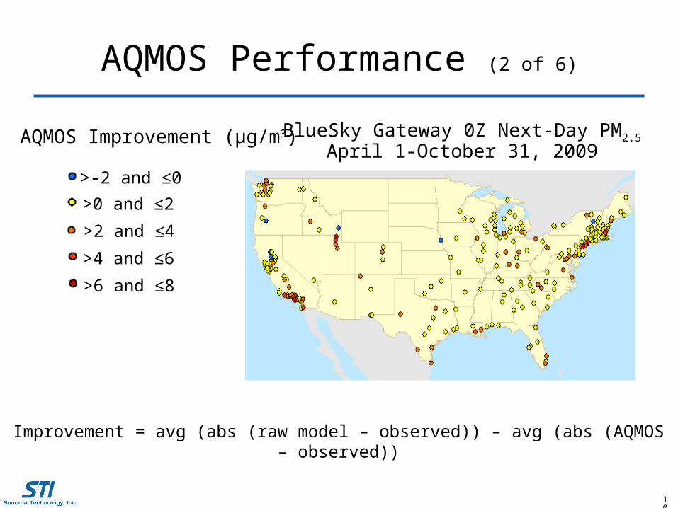
AQMOS Performance (2 of 6)
BlueSky Gateway 0Z Next-Day PM2.5
April 1-October 31, 2009
MOS Improvement (ug/m3)
-1.712867 - 0.000000
0.000001 - 2.000000
2.000001 - 4.000000
4.000001 - 6.000000
6.000001 - 8.000000
MOS Improvement (ug/m3)
-1.712867 - 0.000000
0.000001 - 2.000000
2.000001 - 4.000000
4.000001 - 6.000000
6.000001 - 8.000000
MOS Improvement (ug/m3)
-1.712867 - 0.000000
0.000001 - 2.000000
2.000001 - 4.000000
4.000001 - 6.000000
6.000001 - 8.000000
MOS Improvement (ug/m3)
-1.712867 - 0.000000
0.000001 - 2.000000
2.000001 - 4.000000
4.000001 - 6.000000
6.000001 - 8.000000
MOS Improvement (ug/m3)
-1.712867 - 0.000000
0.000001 - 2.000000
2.000001 - 4.000000
4.000001 - 6.000000
6.000001 - 8.000000
>-2 and ≤0
>0 and ≤2
>2 and ≤4
>4 and ≤6
>6 and ≤8
Improvement = avg (abs (raw model – observed)) – avg (abs (AQMOS – observed))
AQMOS Improvement (µg/m3)

11
AQMOS Performance (3 of 6)
Between April 1-October 31, 2009, AQMOS improved predictions in
CityAQMOS improvement, 6Z NOAA Ozone model (ppb)
Yuba City/Marysville, CA 17.3
York/Chester/Lancaster, PA
15.0
Charleston, SC 13.5
Rock Island-Moline, IL 13.4
East San Gabriel, CA 12.4
. . . . . .
Banning, CA -0.8
Imperial Valley, CA -0.9
Provo, UT -1.2
Washakie Reservation, UT -1.7
Ogden, UT -3.1
Improvement = avg (abs (raw model – observed)) – avg (abs (AQMOS – observed))
• 312 of 326 forecast cities for the next-day NOAA 6Z ozone model
• 239 of 252 forecast cities for the next-day BlueSky Gateway PM2.5 model
12
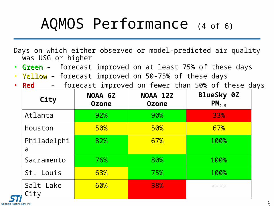
AQMOS Performance (4 of 6)
Days on which either observed or model-predicted air quality was USG or higher • GreenGreen – forecast improved on at least 75% of these days• YellowYellow – forecast improved on 50-75% of these days• RedRed – forecast improved on fewer than 50% of these days
CityNOAA 6Z
OzoneNOAA 12Z
OzoneBlueSky 0Z PM2.5
Atlanta 92% 90% 33%
Houston 50% 50% 67%
Philadelphia 82% 67% 100%
Sacramento 76% 80% 100%
St. Louis 63% 75% 100%
Salt Lake City 60% 38% ----

13
AQMOS Performance (5 of 6)
Atlanta Next-Day 6Z NOAA Ozone ModelApril 1-October 31, 2009
y = 1.3404x
R2 = 0.2704
0
20
40
60
80
100
120
140
0 20 40 60 80 100 120 140
Observed ozone (ppb)
Pre
dic
ted
ozo
ne
(pp
b)
Model
Linear (Model)
y = 0.965x
R2 = -0.0223
0
20
40
60
80
100
120
140
0 20 40 60 80 100 120 140
Observed ozone (ppb)
Pre
dic
ted
ozo
ne
(pp
b)
Model
AQMOS
Linear (Model)
Linear (AQMOS)

14
AQMOS Performance (6 of 6)
Salt Lake City Next-Day 6Z NOAA Ozone ModelApril 1-October 31, 2009
y = 0.9689x
R2 = 0.2133
0
20
40
60
80
100
120
140
0 20 40 60 80 100 120 140
Observed ozone (ppb)
Pre
dic
ted
ozo
ne
(p
pb
)
ModelLinear (Model)
y = 0.9326x
R2 = 0.2906
0
20
40
60
80
100
120
140
0 20 40 60 80 100 120 140
Observed ozone (ppb)
Pre
dic
ted
ozo
ne
(pp
b)
Model
AQMOS
Linear (Model)
Linear (AQMOS)

15
Summary
• AQMOS is available to air quality agencies.• AQMOS should be used in conjunction with other
guidance.• On most days, AQMOS shows improvement over the raw
model output in predicting air quality for specific cities. • AQMOS showed improvement on at least 50% of critical
days in the six cities evaluated.
For more information, please visit http://aqmos.sonomatech.comor contact Dianne Miller