Adjusted empirical likelihood method for quantiles. Inst. Statist. Math. Vol. 55, No. 4, 689-703...
15
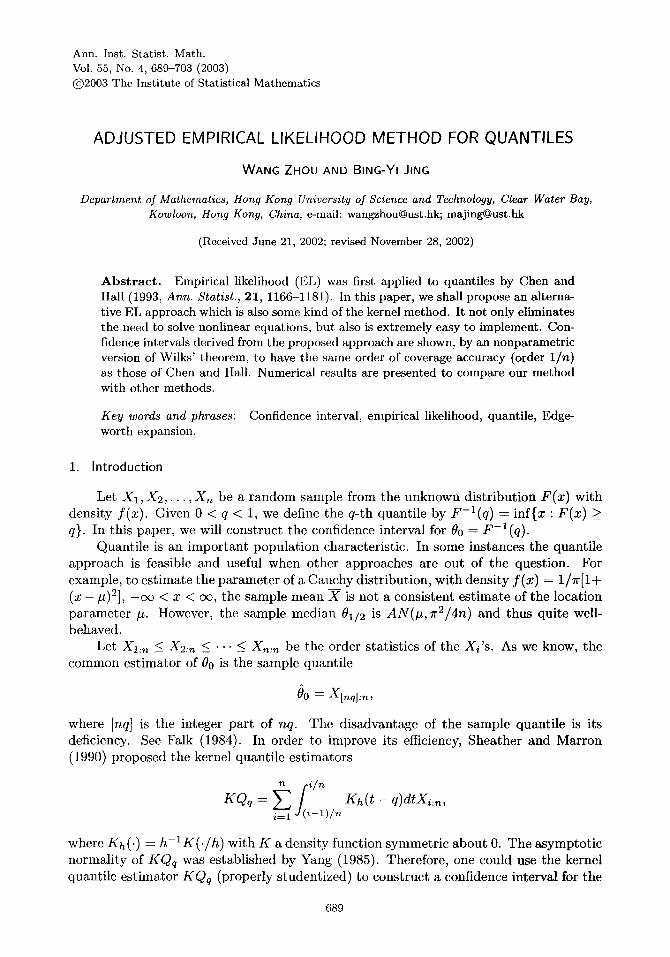
Ann. Inst. Statist. Math. Vol. 55, No. 4, 689-703 (2003) (~)2003 The Institute of Statistical Mathematics ADJUSTED EMPIRICAL LIKELIHOOD METHOD FOR QUANTILES WANG ZHOU AND BING-YI JING Department of Mathematics, Hong Kong University of Science and Technology, Clear Water Bay, Kowloon, Hong Kong, China, e-mail: [email protected]; [email protected] (Received June 21, 2002; revised November 28, 2002) Abstract. Empirical likelihood (EL) was first applied to quantiles by Chen and Hall (1993, Ann. Statist., 21, 1166-1181). In this paper, we shall propose an alterna- tive EL approach which is also some kind of the kernel method. It not only eliminates the need to solve nonlinear equations, but also is extremely easy to implement. Con- fidence intervals derived from the proposed approach are shown, by an nonparametric version of Wilks' theorem, to have the same order of coverage accuracy (order l/n) as those of Chen and Hall. Numerical results are presented to compare our method with other methods. Key words and phrases: Confidence interval, empirical likelihood, quantile, Edge- worth expansion. 1. Introduction Let X1, X2,..., Xn be a random sample from the unknown distribution F(x) with density f(x). Given 0 < q < 1, we define the q-th quantile by F-l(q) = inf{x : F(x) >_ q}. In this paper, we will construct the confidence interval for 0o = F -1 (q). Quantile is an important population characteristic. In some instances the quantile approach is feasible and useful when other approaches are out of the question. For example, to estimate the parameter of a Cauchy distribution, with density f(x) = 1/7r[1+ (x - p)2], -oc < x < 0% the sample mean X is not a consistent estimate of the location parameter #. However, the sample median 01/2 is AN(#,Tr2/4n) and thus quite well- behaved. Let Xl:n _< X2:n <_ "'" <_X,~:n be the order statistics of the Xi's. As we know, the common estimator of 00 is the sample quantile 00 = X[~ql:n, where [nq] is the integer part of nq. The disadvantage of the sample quantile is its deficiency. See Falk (1984). In order to improve its efficiency, Sheather and Matron (1990) proposed the kernel quantile estimators KQq [i/n = Kh(t -- q)dtXi:~, i=l J(i-1)/n where Kh(.) = h-lK(./h) with K a density function symmetric about 0. The asymptotic normality of KQq was established by Yang (1985). Therefore, one could use the kernel quantile estimator KQq (properly studentized) to construct a confidence interval for the 689
Transcript of Adjusted empirical likelihood method for quantiles. Inst. Statist. Math. Vol. 55, No. 4, 689-703...
Ann. Inst. Statist. Math. Vol. 55, No. 4, 689-703 (2003) (~)2003 The Institute of Statistical Mathematics
ADJUSTED EMPIRICAL LIKELIHOOD METHOD FOR QUANTILES
WANG ZHOU AND BING-YI JING
Department of Mathematics, Hong Kong University of Science and Technology, Clear Water Bay, Kowloon, Hong Kong, China, e-mail: [email protected]; [email protected]
(Received June 21, 2002; revised November 28, 2002)
A b s t r a c t . Empirical likelihood (EL) was first applied to quantiles by Chen and Hall (1993, Ann. Statist., 21, 1166-1181). In this paper, we shall propose an alterna- tive EL approach which is also some kind of the kernel method. It not only eliminates the need to solve nonlinear equations, but also is extremely easy to implement. Con- fidence intervals derived from the proposed approach are shown, by an nonparametric version of Wilks' theorem, to have the same order of coverage accuracy (order l /n) as those of Chen and Hall. Numerical results are presented to compare our method with other methods.
Key words and phrases: Confidence interval, empirical likelihood, quantile, Edge- worth expansion.
1. Introduction
Let X1, X2,..., Xn be a random sample from the unknown distribution F(x) with density f(x). Given 0 < q < 1, we define the q-th quantile by F-l(q) = inf{x : F(x) >_ q}. In this paper, we will construct the confidence interval for 0o = F -1 (q).
Quantile is an important population characteristic. In some instances the quantile approach is feasible and useful when other approaches are out of the question. For example, to estimate the parameter of a Cauchy distribution, with density f (x) = 1/7r[1+ (x - p)2], - o c < x < 0% the sample mean X is not a consistent estimate of the location parameter #. However, the sample median 01/2 is AN(#,Tr2/4n) and thus quite well- behaved.
Let Xl:n _< X2:n <_ "'" <_ X,~:n be the order statistics of the Xi's. As we know, the common estimator of 00 is the sample quantile
00 = X[~ql:n,
where [nq] is the integer part of nq. The disadvantage of the sample quantile is its deficiency. See Falk (1984). In order to improve its efficiency, Sheather and Matron (1990) proposed the kernel quantile estimators
KQq [i/n = Kh(t -- q)dtXi:~,
i=l J(i-1)/n
where Kh(.) = h- lK( . /h) with K a density function symmetric about 0. The asymptotic normality of KQq was established by Yang (1985). Therefore, one could use the kernel quantile estimator KQq (properly studentized) to construct a confidence interval for the
689
690 W A N G Z H O U A N D B I N G - Y I J I N G
population quantile 00. However, the coverage of the kernel quantile estimator based confidence interval is not very accurate as our simulation results show.
In the nonparametric case empirical likelihood methods are powerful techniques for constructing confidence intervals and tests, notably in enabling the shape of a confidence region determined by the sample data. Since Owen (1988, 1990) introduced empirical likelihood into statistics, many developments have taken place. For a review, see Owen (2001). When applied to quantiles, Owen's method yields the so-called binomial method confidence intervals. However, because of the discreteness of the binomial distribution, the size of coverage error is of order 0(n-1/2). In order to improve the accuracy, it is natural to use smoothing methods. Chen and Hall (1993) first applied the method of smoothed empirical likelihood to sample quantiles and obtained very accurate results. But their method involves solving a system of nonlinear equations. Adimari (1998) presented a new version of the empirical log-likelihood ratio function for the quantiles which also yielded good results. For other works on application of EL for smoothing problems, we refer to Chert (1996, 1997).
The rest of this paper is arranged as follows. In Section 2, we propose a new version of the empirical likelihood method to quantiles. Based on the asymptotic chisquare distribution of the log-empirical likelihood ratio, we construct confidence intervals for the quantiles. We do some simulations in Section 3 in order to compare all kinds of methods numerically. The proof is deferred to Section 4.
2. Methodology and main results
(2.1)
with
We know that 00 coincides with the M-estimates defined by the equation
~ r O)dF(x) = O, o o
- 1 if z < 0 , r q / ( 1 - q ) if z > 0 .
The empirical likelihood ratio for 0o is
(2.2) R(Oo) =
subject to
(2.3) Pi -> 0, i = 1 , . . . , n ,
Prom (2.2), we have
(2.4) log n(Oo) =
n
sup H(npi) , P l , . . . , P n i=1
n
i = l
- -1 , n
- 0 o ) = 0
i=1
sup ~__,logp~ + n logn , Pl ,...,p,, i=1
where Pi, i = 1 , . . . , n satisfy the constraint (2.3). The method of Lagrange multiplier may be used to maximize }-]i~1 logpi subject to the constraint (2.3). Arguing this, we
EMPIRICAL LIKELIHOOD FOR QUANTILES 691
may prove tha t the maximizat ion point occurs with
1 1 ( 2 . 5 ) = -
n 1 + A(Oo)r - 0o)'
where A(Oo) satisfies the equation
(2.6) -1 ~ r - 0o) n ~ 1 + A(Oo)O(Xi - 0o)
When 00 e [Xl:n , Xn:n] , the solution A(00) of (2.6) is
A(Oo) = (q -- Fn(Oo))/q,
i = l , . . . , n ,
= 0 .
= 2n(F~(Oo) log Fn(O~ + ( 1 - Fn(Oo))log 1 -Fn(O~ --T- i -q
The above formula also appeared in Adimari (1998). From (2.7) log R(00) is a step function with jumps at the observed values. The fact tha t logR(00) can take only a finite number values makes the X 2 approximation not very accurate. It is reasonable to replace Fn(') by some smoothed version of the empirical distribution.
Let the bandwidth be h = hn > 0. Suppose h ~ 0 as n --* oz. Choose some Borel measurable function K(x) as the kernel and define G(t) = f t _ g ( x ) d x . So the smoothed empiricM distr ibution is
( 2 . 8 ) #n(X) : 1 ~ G ( x - x i ) n i=1 h
We propose to use [;n(Oo) in (2.7) instead of Fn(Oo). Thus the adjusted log-empirical likelihood ratio is
(2.9) [(0o) = 2n (Fn(00)log/wn(00) + ( 1 - Fn(Oo))log 1 - Fn(Oo)) q i - - q �9
Clearly, our [(0o) has a closed form, while Chen and Hall's version is implicitly deter- mined by a nonlinear equation. In order to state our theorem, we give some regularity conditions.
(i) Let f (x) = F'(x). For some integer r > 2, f and f(r -1) exist in a neighborhood of 00, and are continuous at 00. Also f(Oo) > O.
(ii) The kernel K( . ) is bounded and has a compact support [a, b]. For some decomposition, a = u0 < ul < - . . < u m = b, K(.) is either strictly posi- tive or strictly negative on each interval (uj-1 , uj), where j = 1 , . . . , m. Also suppose
f uK(u)a(u)du = O,
1, j = 0 , uJK(u)du = O, <_ j <_ rl - 1, 1
C, j ----- r l ,
n where Fn is the empirical distr ibution function given by Fn(x) = • }-]~=1 I{Xi < x}, n with I{.} being the indicator function. Hence the log-empirical likelihood ratio is
(2.7) l(Oo) = - 2 log R(Oo)
692 WANG ZHOU AND BING-YI JING
where C is some finite constant and rl is some integer greater than or equal to r.
(iii) n h / l o g n ---+ oc, nh 2 is bounded as n --~ oc. Let us give some remarks about the conditions. The first requires that the distribu-
tion function F be sufficiently smooth in a neighborhood of 00. That f(80) > 0 guaran- tees the asymptotic variance of the sample quantile is of order n -1 . Without that assump- tion, the asymptotic theory is quite different. We refer to Feldman and Tucker (1966). The second condition specifies that K(.) is different from the commonly used kernel in
nonparametric density estimation. For example, K(u) = { ~ u 2 + -3+~v~ }I([u] <_ 1) satisfies condition (ii) with rl = 2. Finally, condition (iii) implies that the bandwidth h does not converge to zero too fast or too slowly.
THEOREM 2.1. Let [(0o) be defined by (2.9). Assume that conditions (i)-(iii) hold. Then we have as n ~ oo,
P([(Oo) <_ x) - P(X~ <- x) = O(71, -1 )
for each fixed x.
We postpone the proof of Theorem 2.1 to Section 4. By Theorem 2.1, we have
lim P{Oo e Ihc} = P(X 2 <_ c), n ---+ O 0
where Ihc = {0 : [(0) <_ c}. If c is chosen to satisfy P(X~ -< c) = a, then the coverage probability of the interval Ih~ will approximate a with error O(n -1) as n --+ oo. Also note that our result is not uniform in x.
3. Simulation results
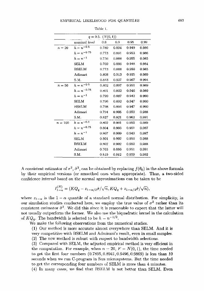
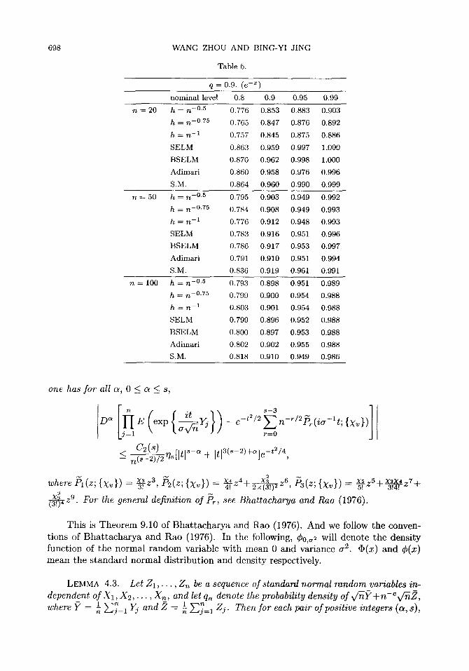
A Monte Carlo study was conducted to investigate the coverage accuracy of empiri- cal likelihood confidence interval. We generated 10,000 pseudo random samples of various sizes from standard normal, exponential and chi-square with degree 1 respectively. The kernel function K has been chosen to be K(u) = { 21-9'/7iu2+ - a + ~ } I ( l u I < 1), which
satisfies condition (ii) with r = 2. And we employed bandwidths h = n -1/2, n -3/4, n -1, where h = n -1/2 satisfies condition (iii).
Also shown in Tables 1-6 are smoothed empirical likelihood method (SELM) pro- posed by Chen and Hall (1993) and Bartlett adjusted SELM (BSELM) respectively. In this case, we use K(u) = 15 _ _ n-3/4. ~ (1 -- u2)2I(lu] < 1), and h = Adimari's result (1998) is included too for comparison.
Confidence intervals by the normal approximation method, denoted by S.M. in Tables 1-6, can be obtained as follows. From Yang (1985), we know
nl /2 (KQq - Oo) --+L N(O, or2),
where
( 3 . 1 ) _ p ( 1 - f 2 ( O o ) �9
E M P I R I C A L LIKELIHOOD F O R Q U A N T I L E S
T a b l e 1.
q = 0.5. (N(0, 1)) n o m i n a l l e v e l 0.8 0.9 0.95 0.99
n = 2 0 h = n - ~ 0.789 0.894 0.949 0.986
h = n - ~ 0.773 0.891 0.953 0.986
h = n - 1 0.756 0.888 0.955 0.985
S E L M 0.769 0.886 0.948 0.984
B S E L M 0.773 0.888 0.950 0.985
A d i m a r i 0.808 0.913 0.925 0.989
S.M. 0.843 0.927 0.967 0.994
n = 50 h = n - ~ 0.802 0.897 0.951 0.989
h = n - ~ 0.801 0.892 0.946 0.989
h = n - 1 0.799 0.887 0.942 0.990
S E L M 0.796 0.892 0.947 0.990
B S E L M 0.798 0.894 0.947 0.990
A d i m a r i 0.794 0.905 0.950 0.988
S.M. 0.827 0.921 0.962 0.991
n = 100 h -- n - ~ 0.802 0.901 0.950 0.989
h = n - 0 7 5 0.804 0.903 0.951 0.987
h -- n - 1 0.807 0.909 0.949 0.987
S E L M 0.801 0.902 0.950 0.988
B S E L M 0.802 0.902 0.950 0.988
A d i m a r i 0.763 0.886 0.951 0.991
S.M. 0.819 0.912 0.959 0.992
693
A consistent estimator of a 2, &2, can be obtained by replacing f(00) in the above formula by their empirical versions (or smoothed ones when appropriate). Thus, a two-sided confidence interval based on the normal approximations can be taken to be
rl (N) = (KQ - +
where Zl_c~ is the 1 - a quantile of a standard normal distribution. For simplicity, in our simulation studies conducted here, we employ the true value of a 2 rather than its consistent estimator &2. We did this since it is reasonable to expect that the latter will not usually outperform the former. We also use the biquadratic kernel in the cMculation of KQq. The bandwidth is selected to be h = n -1/2.
We make the following observations from the numerical studies. (1) Our method is more accurate almost everywhere than SELM. And it is very competitive with BSELM and Admirani's result, even in small samples. (2) The new method is robust with respect to bandwidth selections. (3) Compared with SELM, the adjusted empirical method is very efficient in the computation. For example, when n = 20, F = N(0, 1), the time needed to get the first four numbers (0.7895, 0.8941, 0.9496, 0.9869) is less than 10 seconds when we run C-program in Sun microsystems. But the time needed to get the corresponding four numbers of SELM is more than 4 minutes. (4) In many cases, we find that BSELM is not better than SELM. Even
694 WANG ZHOU AND BING-YI JING
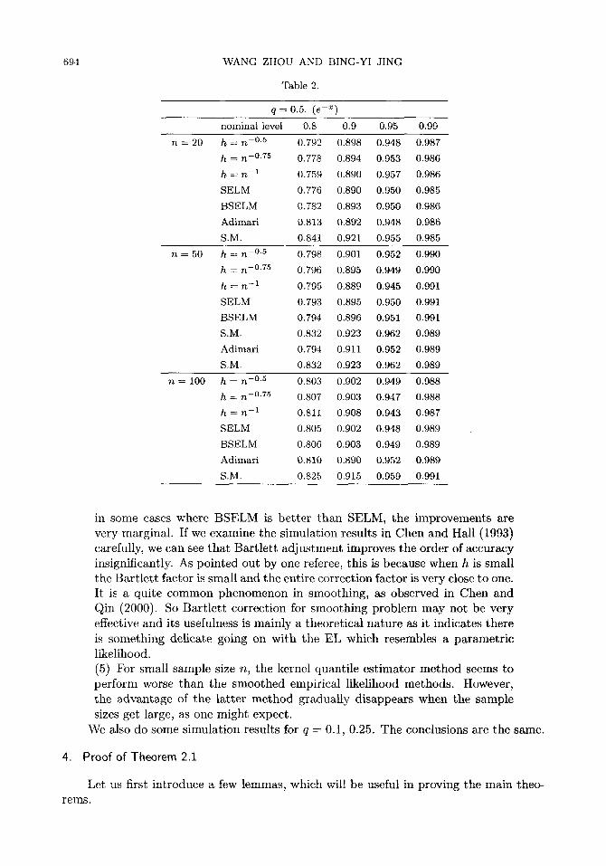
Table 2.
q = 0.5. (e - x )
nominal level 0.8 0.9 0.95 0.99
n = 20 h = n - ~ 0.792 0.898 0.948 0.987
h = n -~ 0.778 0.894 0.953 0.986
h = n -1 0.759 0.890 0.957 0.986
SELM 0.776 0.890 0.950 0.985
BSELM 0.782 0.893 0.950 0.986
Adimari 0.813 0.892 0.948 0.986
S.M. 0.841 0.921 0.955 0.985
n = 5 0
n = 100
h = n - ~ 0.798 0.901 0.952 0.990
h = n -0"75 0.796 0.895 0.949 0.990
h = n -1 0.795 0.889 0.945 0.991
SELM 0.793 0.895 0.950 0.991
BSELM 0.794 0.896 0.951 0.991
S.M. 0.832 0.923 0.962 0.989
Adimari 0.794 0.911 0.952 0.989
S.M. 0.832 0.923 0.962 0.989
h = n -~ 0.803 0.902 0.949 0.988
h = n -~ 0.807 0.903 0.947 0.988
h = n -1 0.811 0.908 0.943 0.987
SELM 0.805 0.902 0.948 0.989
BSELM 0.806 0.903 0.949 0.989
Adimari 0.810 0.890 0.952 0.989
S.M. 0.825 0.915 0.959 0.991
in some cases where B S E L M is b e t t e r t h a n SELM, t he i m p r o v e m e n t s are
very m a r g i n a l . If we e x a m i n e the s i m u l a t i o n r e su l t s in C h e n a n d Hal l (1993)
carefully, we can see t h a t B a r t l e t t a d j u s t m e n t improves t he o rder of a c c u r a c y
ins igni f icant ly . As p o i n t e d ou t by one referee, th i s is because w h e n h is smal l
t he B a r t l e t t factor is sma l l a n d the en t i r e cor rec t ion fac tor is very close to one.
I t is a qu i t e c o m m o n p h e n o m e n o n in s m o o t h i n g , as obse rved in C h e n a n d
Q i n (2000). So B a r t l e t t co r rec t ion for s m o o t h i n g p r o b l e m m a y no t be very
effective a n d i ts usefu lness is m a i n l y a theore t i ca l n a t u r e as it i nd ica t e s t he re
is s o m e t h i n g de l ica te go ing on w i t h the EL which resembles a p a r a m e t r i c
l ikel ihood.
(5) For smal l s ample size n , t he ke rne l q u a n t i l e e s t i m a t o r m e t h o d seems to
p e r f o r m worse t h a n the s m o o t h e d empi r i ca l l ike l ihood m e t h o d s . However ,
t he a d v a n t a g e of t he l a t t e r m e t h o d g r a d u a l l y d i s a p p e a r s w h e n the s a m p l e
sizes get large, as one migh t expect .
We also do some s i m u l a t i o n resu l t s for q = 0.1, 0.25. T h e conc lus ions are the same.
4. Proof of Theorem 2.1
Let us first i n t r o d u c e a few l emmas , which will be useful in p r ov i ng the m a i n theo-
rems.
E M P I R I C A L L I K E L I H O O D F O R Q U A N T I L E S
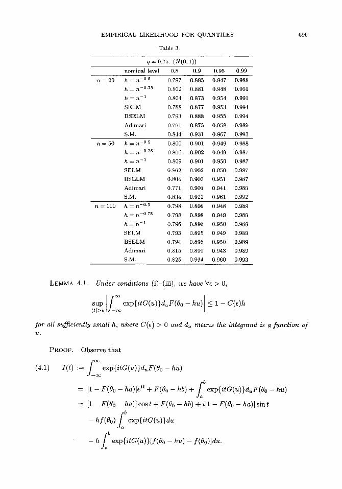
Table 3.
q = 0.75. (N(O, 1))
n o m i n a l l e v e l 0.8 0.9 0.95 0.99
n = 2 0 h = n -~ 0.797 0.885 0.947 0.988
h = n -~ 0.802 0.881 0.948 0.991
h = n -1 0.804 0~873 0.954 0.991
SELM 0.788 0.877 0.953 0.994
B S E L M 0.793 0.888 0.955 0.994
Adimar i 0.791 0.875 0.958 0.989
S.M. 0.844 0.931 0.967 0.993
n = 5 0 h = n - ~ 0.800 0.901 0.949 0.988
h = n -~ 0.806 0.902 0.949 0.987
h = n -1 0.809 0.901 0.950 0.987
SELM 0.802 0.902 0.950 0.987
B S E L M 0.804 0.903 0.951 0.987
Adimar i 0.771 0.901 0.941 0.989
S.M. 0.834 0.922 0.961 0.992
n = 100 h = n -~ 0.798 0.898 0.948 0.989
h = n - ~ 0.798 0.898 0.949 0.989
h -- n - 1 0.796 0.896 0.950 0.989
SELM 0.793 0.895 0.949 0.989
B S E L M 0.794 0.896 0.950 0.989
Adimar i 0.815 0.891 0.943 0.989
S.M. 0.825 0.914 0.960 0.993
695
LEMMA 4.1. Under conditions (i) (iii), we have Ve > 0,
sup / ~ exp{itG(u)}d~,F(Oo - hu) <_ 1 - C(e)h I t q > ~
for all sufficiently small h, where C(e) > 0 and d~ means the integmnd is a function of U.
PROOF. Observe t h a t
(4.1) I(t) := exp{itG(u)}d~F(Oo - hu) 0 ( 3
= [1 - F ( O o - ha)]e ~t + F(Oo - h b ) + exp{ita(u)}duF(Oo - h u )
= [1 - F ( O o - h a ) ] c o s t + F ( O o - h b ) + i [ 1 - F ( O o - h a ) ] s i n t
- hf(Oo) .~b exp{itG(u)}du
- h f b exp{itG(u)}[f(Oo - hu) - f(Oo)]du. Ja
696 W A N G Z H O U A N D B I N G - Y I J I N G
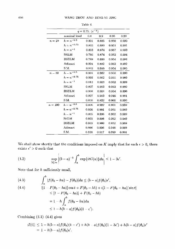
Tab le 4.
q = 0.75. (e -x )
n o m i n a l level 0.8 0.9 0.95 0.99
n = 20 h = n - ~ 0.801 0.885 0.950 0.990
h = n -0"75 0.803 0.880 0.951 0.991
h = n - 1 0.803 0.874 0.957 0.993
S E L M 0.786 0.874 0.952 0.994
B S E L M 0.789 0.883 0.954 0.994
A d i m a r i 0.804 0.892 0.962 0.992
S.M. 0.842 0.916 0.954 0.985
n = 50
n = 100
h = n - ~ 0.804 0.902 0.950 0.990
h = n - ~ 0.809 0.902 0.951 0.989
h = n - 1 0.812 0.903 0.952 0.989
S E L M 0.807 0.903 0.953 0.990
B S E L M 0.808 0.904 0.954 0.990
A d i m a r i 0.807 0.903 0.946 0.991
S.M. 0.830 0.922 0.961 0.990
h = n -~ 0.806 0.902 0.951 0.989
h = n - ~ 0.806 0.901 0.951 0.989
h = n - 1 0.805 0.898 0.952 0.989
S E L M 0.803 0.898 0.952 0.989
B S E L M 0.803 0.900 0.952 0.989
A d i m a r i 0.806 0.896 0.948 0.989
S.M. 0.828 0.917 0.959 0.991
We shall show shortly tha t the conditions imposed on K imply that for each c > 0, there exists c' > 0 such that
f (4 .2 ) s u p (b - a) - 1 exp{ita(u)}du [ t l>e
Note that for h sufficiently small,
(4.3)
(4.4)
< 1 - 3~'.
b a I f (O o - h u ) - f ( O o ) l d u < ( b - a ) f ( O o ) d ,
111 - F(Oo - ha)] cost + F(Oo - hb) + i[1 - F(Oo - ha)] s in t I
_< [1 - F(Oo - ha)] + F(Oo - hb)
f = 1 - h f (Oo - h u ) d u
<_ 1 - h ( b - a ) f ( O o ) ( 1 - e ' ) .
Combining (4.1)-(4.4) gives
I I ( t ) l <_ 1 - h ( b - a ) f ( O o ) ( 1 - ~') + h ( b - a ) f ( O o ) ( 1 - 3e') + h ( b - a ) f ( O o ) d
= 1 - h ( b - a ) f (Oo)e ' .
E M P I R I C A L LIKELIHOOD F O R Q U A N T I L E S
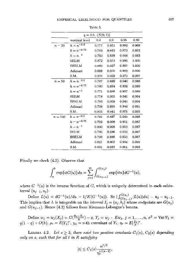
Table 5.
q = 0.9. (N(0, 1))
nominal level 0.8 0.9 0.95 0.99
n = 20 h = n - ~ 0.777 0.851 0.886 0.908
h = n -0'75 0.769 0.842 0.873 0.893
h = n -1 0.760 0.838 0.868 0.883
SELM 0.872 0.954 0.995 1.000
BSELM 0.880 0.957 0.997 1.000
Adimar i 0.888 0.956 0.983 0.996
S.M. 0.834 0.929 0.972 0.997
n = 5 0 h = n - ~ 0.787 0.889 0.940 0.988
h = n - ~ 0.780 0.894 0.938 0.989
h -- n -1 0.771 0.896 0.937 0.989
SELM 0.778 0.905 0.941 0.994
BSELM 0.783 0.908 0.944 0.994
Adimar i 0.798 0.895 0.940 0.991
S.M. 0.855 0.941 0.975 0.995
n = 100 h = n - ~ 0.792 0.897 0.949 0.988
h = n -~ 0.793 0.900 0.951 0.987
h = n - 1 0.800 0.900 0.953 0.987
SELM 0.796 0.896 0.950 0.987
BSELM 0.799 0.898 0.950 0.987
Adimar i 0.821 0.902 0.934 0.992
S.M. 0.831 0.922 0.961 0.993
697
F i n a l l y w e c h e c k (4 .2 ) . O b s e r v e t h a t
~.ab m rG(u~) exp{itG(u)}du ---- j~l= ]G(~j_I) exp{i tu}dG-l(u) '
w h e r e G-l(u) is t h e i n v e r s e f u n c t i o n o f G , w h i c h is u n i q u e l y d e t e r m i n e d i n e a c h s u b i n -
t e r v a l (uj-1, uj). f G(u~) D e f i n e L(u) = dG- l (u) /du = 1/K(G-I(u)) . S o I a ( ~ j _ ~ ) [ L ( u ) l d u l = u ~ - U i _ l .
T h i s i m p l i e s t h a t L is i n t e g r a b l e o n t h e i n t e r v a l Ij = (aj, bj) w h o s e e n d p o i n t s a r e G(uj) a n d G(Uj_l). H e n c e (4 .2 ) f o l l o w s f r o m R i e m a n n - L e b e s g u e ' s l e m m a .
D e f i n e wj = wj(Xj) = G ( ~ ) - q, Yj = wj - Ewj, j = 1, . . . , n , a 2 = V a r Y 1 =
q (1 - q) + O ( h ) , Pr = E [ Y I [ r , Xv = v - t h c u m u l a n t o f Y1, ~ r = E l ~ [ ~.
L E M M A 4.2. Let s > 3, there exist two positive constants C 1 ( 8 ) , 6 2 ( 8 ) depending only on s, such that for all t in R satisfying
nl/2 Itl < 61(s) 1/(8_2),
qs
698 W A N G Z H O U A N D B I N G - Y I J I N G
Table 6.
q = 0 . 9 . (e - x )
nomina l leve! 0.8 0.9 0.95 0.99
n = 20 h = n - ~ 0.776 0.853 0.883 0.903
h = n -0"75 0.765 0.847 0.876 0.892
h = n -1 0.757 0.845 0.875 0.886
SELM 0.863 0.959 0.997 1.000
BSELM 0.870 0.962 0.998 1.000
Adimar i 0.860 0.958 0.976 0.996
S.M. 0.864 0.960 0.990 0.999
n = 5 0
n = 100
h = n - ~ 0.795 0.903 0.949 0.992
h = n -0 '75 0.784 0.908 0.949 0.993
h ---- n - 1 0.776 0.912 0.948 0.993
SELM 0.783 0.916 0.951 0.996
B S E L M 0.786 0.917 0.953 0.997
Adimar i 0.791 0.910 0.951 0.994
S.M. 0.836 0.919 0.961 0.991
h = n -~ 0.793 0.898 0.951 0.989
h = n -0-75 0.799 0.900 0.954 0,988
h = n -1 0.803 0.901 0,954 0.988
SELM 0.799 0.896 0.952 0.988
B S E L M 0.800 0.897 0.953 0.988
Adimar i 0.802 0.902 0.955 0.988
S.M. 0.818 0.910 0.949 0.986
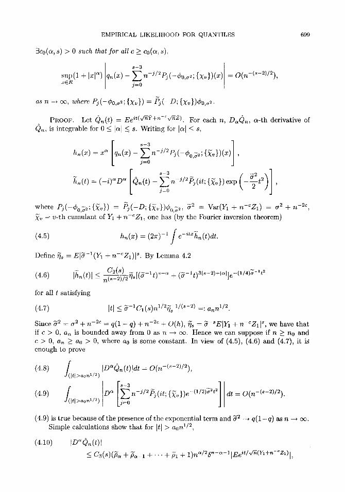
one has for all (~, 0 < c~ < s,
E e x p [ a v f ~ 3 j ) - E n - ~ / 2 [ ) ~ ( i a - l t ; { x ~ } ) r = 0
C 2 ( s ) ~Ts[itls_ a + i t[3(s_2)+a]e_t2/4 ' -- n (S -2 ) /2
where P l ( z ; { X v } ) = 3z3 2 , 2(z; { X v } ) = 4_4_ = -4T. t ~ ~ - ~ ~ 5! - - 3 ! 4 ! ~ - -
x~ ~9 For the general definition of tSr, see Bhattacharya and Rao (1976). - ~ .
This is Theorem 9.10 of Bhattacharya and Rao (1976). And we follow the conven- tions of Bhattacharya and Rao (1976). In the following, r will denote the density function of the normal random variable with mean 0 and variance a s. O(x) and r mean the standard normal distribution and density respectively.
LEMMA 4.3. Let Z1, . . . , Zn be a sequence of standard normal random variables in- dependent of X1, X 2 , . . . , Xn, and let qn denote the probability density of v/-nY + n-Cvfn~7 ,
n 1 n where 1) = ~ E j = I YJ and 2 = ~ E j = I Z j . Then for each pair of positive integers (c~, s),
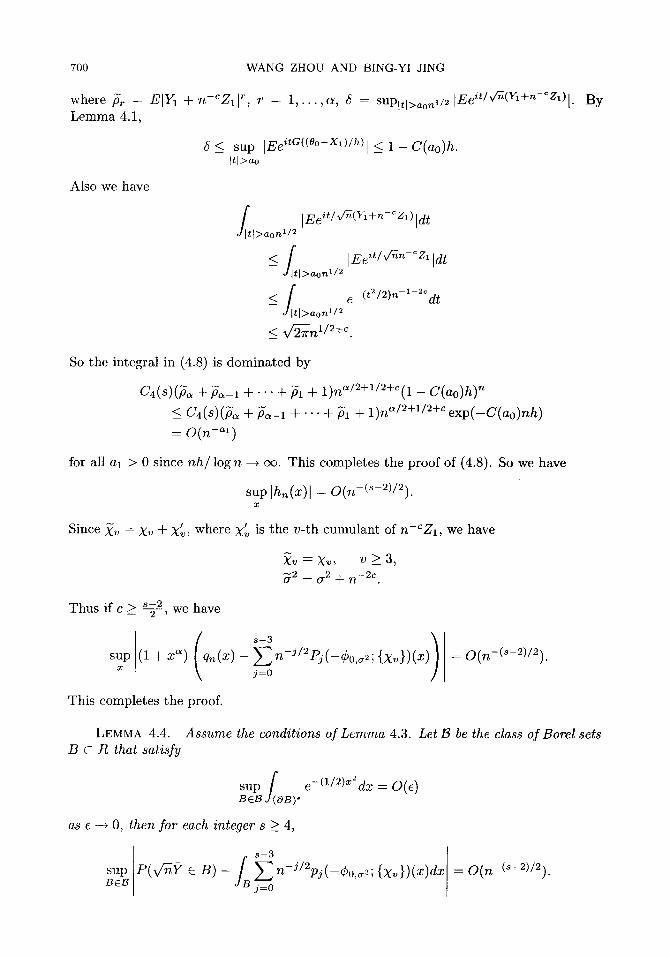
EMPIRICAL LIKELIHOOD FOR QUANTILES 699
3co(a, s) > 0 such that for all c > Co(a, s),
q n ( x ) s--3 sup(1 § I~] ~) - ~ n-J/~Pj(-r {X.})(x) xCR j=0
as n -* oo, where Pj(-r {Xv}) = P j ( - D ; {X~})r
= 0 ( n - ( ~ - 2 ) / 2 ) ,
PROOF. Let Qn(t) -- Ee it(v~9+n-~/-~2). For each n, D~Q~, a - th derivative of Q~, is integrable for 0 _< [a[ < s. Writ ing for [a I _< s,
s - 3
h n ( x ) = x ~ an(X) - E n - J / 2 p j ( - r ; {~v})(x) , j=o
hn(t) = ( - i ) " D " Qn(t) - E n - J / 2 p J ( i t ; {:~v})exp - t 2 , j=O
where P j ( - r {Xv}) = P j ( - D ; {~})0o , ;2 , y2 _ _ Var(Y1 + n - c z i ) ~-- 0 .2 "4- n -2c, ~ =- v-th cumulant of Y1 + n-~Z1, one has (by the Fourier inversion theorem)
(4.5) hn(x) = (27r) -1 f f e-UZhn(t)dt.
Define ~ -- EI~-I(Y1 + n-cZ1)[ s. By Lemma 4.2
C2(s) ~ s [ ( ~ _ l t ) s _ ~ ~- ( ~ _ l t ) 3 ( s _ 2 ) + l a l ] e _ ( 1 / 4 ) a - l t 2 n (S -2 ) / 2
Itl <_ ~ - l C l ( 8 ) l t 1 / 2 ~ s 1 / ( s - 2 ) =: ann 1/2.
Since ~2 = a2 + n-2C __ q(1 - q) + n -2c + O(h), ~s = ~5-sEIY1 + n-cZ11 s, we have tha t if c > 0, an is bounded away from 0 as n -~ co. Hence we can suppose if n > no and c > 0, an ~ ao > 0, where ao is some constant. In view of (4.5), (4.6) and (4.7), it ig enough to prove
(4.8) ~ /Itl>aoMI2) [D~Q~(t)ldt = O(n-(S-2)/2)'
dt = O ( n - ( S - 2 ) / 2 ) . (4.9) /[tl>aonl/2) k j--~
(4.9) is true because of the presence of the exponential term and ~2 _. q ( 1 - q ) as n ~ c~. Simple calculations show tha t for [t[ > aon 1/2,
(4.10) [D~Q~(t)[
C3(8)(Pa -~-Pa--1 -[-"""-[-F1 -[- 1)n'~/25n-<~-'lEe~t/'g-~(Y'+n-:z')[,
(4.6) Ihn(t)] _<
for all t satisfying
(4.7)
700 WANG ZHOU AND BING-YI JING
where fir = ElY1 + n-cZl[ r, r = 1, . . . , (~, 5 = suPltl>aon~/2 [Eeit/v~(Y'+n-r Lemma 4.1,
Also we have
8 < sup [tl>ao
lEe itc((~176 < 1 - C(ao)h.
By
J(Itl>aonm/2 [Eeit / ~ ( Y~ +n-c zo [dt
< f [Ee it/'J-~n-cZ~ [dt Ylt [>aonl/~
O~ltl>aont/2 e-(t2/2)n-1-2Cdt
< v '~n l /2+ c.
So the integral in (4.8) is domina ted by
C4(8)(pc~ -+- Pc~-, -~-"""-~- Pl -J- 1)na/2+1/2+c(1 - C(ao)h) u
< C4(s)(~fi~ + "fi~-I + " " + ~fil + 1)n~/~+l/a+Cexp(-C(ao)nh) = o ( ~ - o , )
for all al > 0 since nh/log n ~ ~ . This completes the proof of (4.8). So we have
sup [hn(x)] ~- O(n-(S-2)/2). x
Since ~ , = X, + X~, where X~ is the v- th cumulant of n-~Z1, we have
X~ = X~, v > 3 , ~2 = (72 _~_ n-2c .
Thus if c > ~-~, we have
,1 ( 3 ) sup + ~ ) q~(x) - ~ n - J / ~ P ~ ( - r { ~ v I ) ( x ) = O(n- (~-~) /~) .
x j=O
This completes the proof.
LEMMA 4.4. Assume the conditions of Lemma 4.3. Let I3 be the class of Borel sets B C R that satisfy
sup f e-O/2)~2dx = 0(~) BeB J (OB)"
as e --~ 0, then for each integer s > 4,
sop c B) - ~ - J / ' p j ( - r {>C,})(x)d~ = O(~-( ' -W') . BCI3 j=O
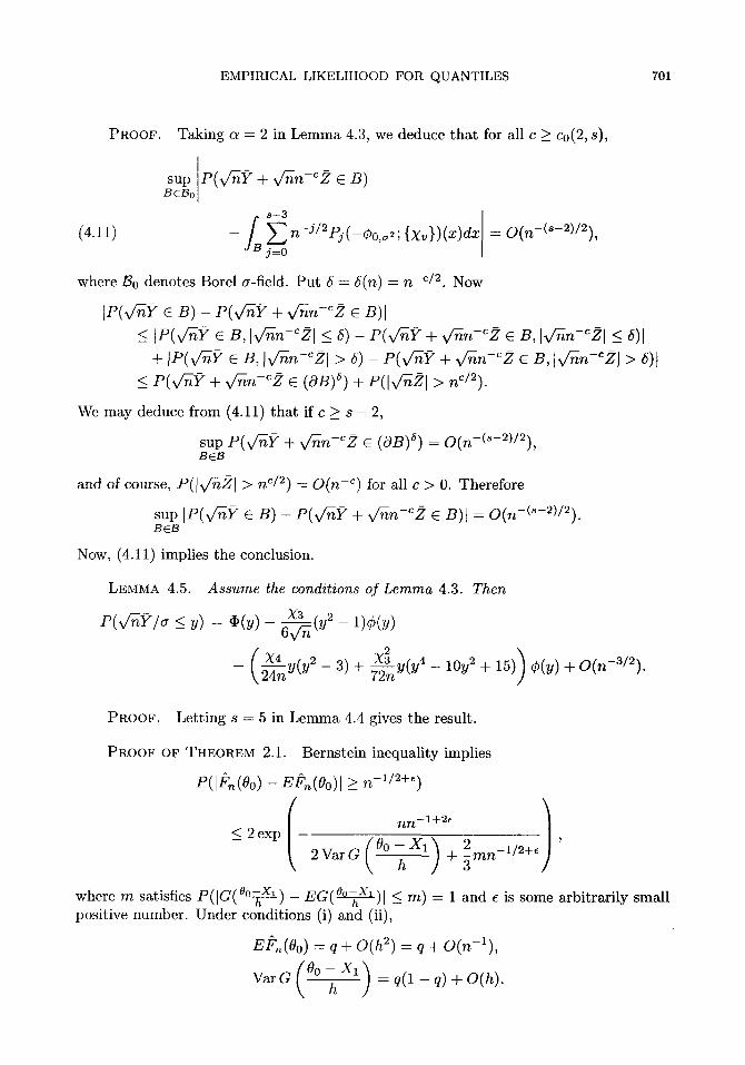
EMPIRICAL LIKELIHOOD FOR QUANTILES 701
(4.11)
PROOF. Taking a = 2 in Lemma 4.3, we deduce tha t for all c >_ c0(2, s),
sup P ( v ~ f " + v ~ n - ~ 2 �9 B) BC/~o
8--3 - Jfs E n - J / 2 p j ( - r 1 7 6 1 7 6 {XvI)(x)dx = O(n-(S-2)/2),
j=O
where B0 denotes Borel a-field. Pu t 5 = 5(n) = n -~/2. Now
IP(v~17 �9 B) - P (v /~ l ) + v ~ n - ~ 2 �9 B)I
_< IP(v~Y �9 B, [v/-~n-C21 < 5) - r ( v / ~ + v~n-C2 �9 B, Iv~n-~21 ~ ~)l + I P ( v ~ ? �9 B, Iv/-~n-~21 > 5) - P(v/-~f " + v ~ n - C 2 �9 B, Iv/-~n-C2] > 5)t
<_ P(v/-~f " + v '~n-~2 �9 (OB) ~) + P(Iv~21 > nC/2). We may deduce from (4.11) tha t if c >_ s - 2,
sup P(v/-~f " + v/-~n-C2 �9 (OB) ~) = 0(n-(8-2)/2), BEt3
and of course, P ( I v ~ 2 1 > n ~/2) = O(n -~) for all c > 0. Therefore
sup I P ( v ~ Y �9 B) - P ( v ~ Y + v ~ n - ~ 2 �9 B)I = O(n-(S-2)/2). BCB
Now, (4.11) implies the conclusion.
LEMMA 4.5. Assume the conditions of Lemma 4.3. Then
P(v/-n?/a < y) = (I)(y) - 6-~nn (y 2 - 1)r
/' x4 , 2 )r ) - k-2-~nYiY - 3) + ~ n y ( y 4 - 10y 2 + 15) r + O(tt-3/2).
PROOF. Let t ing s = 5 in Lemma 4.4 gives the result.
PROOF OF THEOREM 2.1. Bernstein inequality implies
P(IF'n(Oo) - EFn(Oo)I >_ n -1/2+e)
~2exp ( 0 o _ X l ) ~ , 2 Var G -~ + - m n -1/2+~
where m satisfies P ( I G ( ~ - ~ ) - EG(-~- - - ) I _ m) = 1 and e is some arbitrari ly small positive number. Under conditions (i) and (ii),
E[~n(Oo) = q + O(h 2) = q + O(n-1) ,
V~ra(~ h = q(1 - q) + O(h).
702 WANG ZHOU AND BING-YI JING
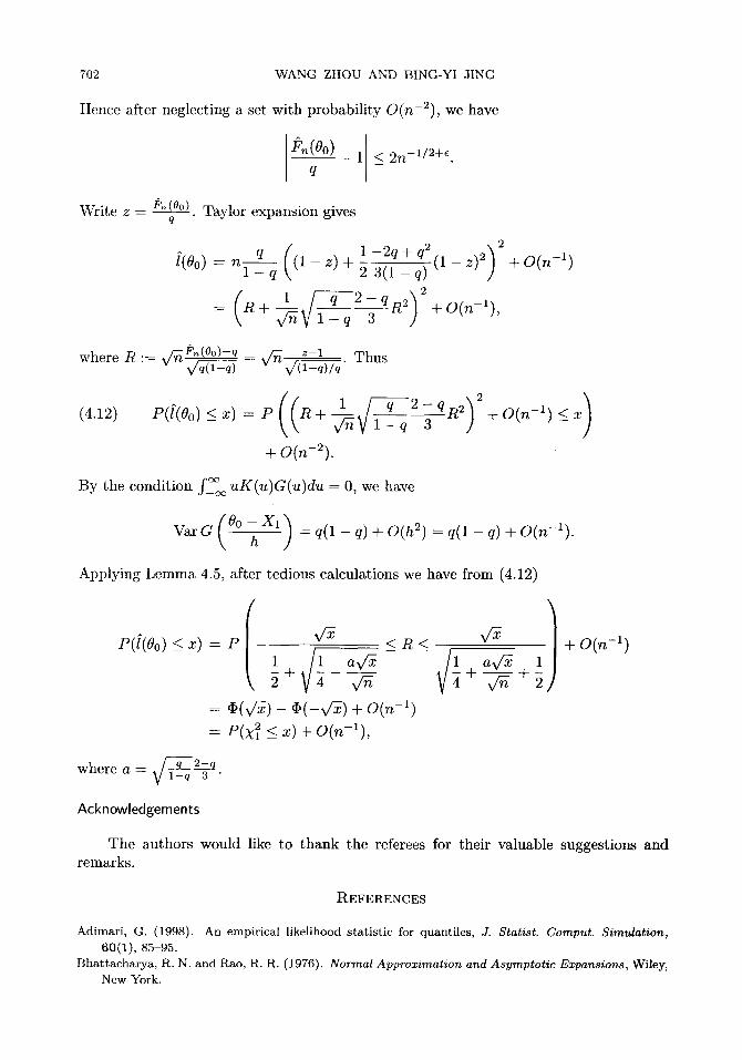
Hence after neglecting a set with probabili ty O(n-2) , we have
Write z - ~ . ( O o ) q
�9 nk-oj 1 ~ 2 n -1/:+r q
�9 Taylor expansion gives
1 - 2 q + q2 [(0o) = n q------~- (1 - z) +
1 - q 2 3 ( 1 - q )
1 . _ / ~ _ 2 - q R 2 ) 2 = ( n + ~ g y - ~ 5
z-I �9 Thus where R /~ ~n(Oo)-q _ _ , / ~ z-1 : : X/rt ~ v "~v/(l_q)/q
(1 -z) 2)
+ O(n-1),
(4�9
+ O(n -1)
1 . _/-~-~_2- q R 2 P([(Oo) <_ x) = P R + " ~ V 1 - : q 5 + O ( n - 1 ) ~ x
+ O(~-2)�9
By the condit ion f ' ~ u K ( u ) G ( u ) d u = 0, we have
V a r G ( O ~ = q(X - q) + O(h 2) = q(X - q) + O(n-1) .
Applying Lemma 4.5, after tedious calculations we have from (4.12)
P([(Oo) <_ x) = P v~ _<n< v~ ) 1 ~1 av/~ 11 av~ 1 2+ 4 V~ 4+-~-+2
= ~ ( v ~ ) - ~ ( - v ~ ) + o (n -1) -- P ( x 2 < x ) + O ( n - 1 ) ,
where a = l ~ _ q 23q�9
Acknowledgements
-4- O(n -1)
Adimari, G. (1998). An empirical likelihood statistic for quantiles, J. Statist. Comput. Simulation, 60(1), 85-95.
Bhattacharya, R. N. and Rao, R. R. (1976). Normal Approximation and Asymptotic Expansions, Wiley, New York.
REFERENCES
The authors would like to thank the referees for their valuable suggestions and remarks�9
EMPIRICAL LIKELIHOOD FOR QUANTILES 703
Chen, S. (1996). Empirical likelihood confidence intervals for nonparametric density estimation, Biometrika, 83(2), 329~41.
Chen, S. (1997). Empirical likelihood-based kernel density estimation, Austral. J. Statist., 39(1), 47-56. Chen, S. and Hall, P. (1993). Smoothed empirical likelihood confidence intervals for quantiles, Ann.
Statist., 21(3), 1166-1181. Chen, S. and Qin, Y. (2000). Empirical likelihood confidence intervals for local linear smoothers,
Biometrika, 87(4), 946 953. Falk, M. (1984). Relative deficiency of kernel'type estimators of quantiles, Ann. Statist., 12(1), 261-268. Feldman, D. and Tucker, H. G. (1966). Estimation of non-unique quantiles, Ann. Math. Statist., 37(2),
451-457. Owen, A. B. (1988). Empirical likelihood ratio confidence intervals for a single functional, Biometrika,
7.5(2), 237-249. Owen, A. B. (1990). Empirical likelihood ratio confidence regions, Ann. Statist., 18(1), 90-120. Owen, A. B. (2001). Empirical Likelihood, Chapman and Hall, London. Sheather, S. J. and Matron, J. S. (1990). Kernel quantile estimators, J. Amer. Statist. Assoc., 85(410),
410-416. Yang, S. S. (1985). A smooth nonparametric estimator of a quantile function, J. Amer. Statist. Assoc.,
80(392), 1004-1011.