Adaptive Robust Control Under Model Uncertainty

Tomasz R. Bielecki a, Tao Chen, a Igor Cialenco, a Areski Cousin b, Monique Jeanblanc c

First Circulated: June 06, 2017

Abstract: In this paper we propose a new methodology for solving an uncertain stochastic Marko-vian control problem in discrete time. We call the proposed methodology the adaptiverobust control. We demonstrate that the uncertain control problem under considerationcan be solved in terms of associated adaptive robust Bellman equation. The success ofour approach is to the great extend owed to the recursive methodology for constructionof relevant confidence regions. We illustrate our methodology by considering an opti-mal portfolio allocation problem, and we compare results obtained using the adaptiverobust control method with some other existing methods.

Keywords: adaptive robust control, model uncertainty, stochastic control, dynamic programming,recursive confidence regions, Markov control problem, portfolio allocation.

MSC2010: 93E20, 93E35, 49L20, 60J05

1 Introduction

In this paper we propose a new methodology for solving an uncertain stochastic Markovian con-trol problem in discrete time, which is then applied to an optimal portfolio selection problem.Accordingly, we only consider terminal optimization criterion.

The uncertainty in the problem comes from the fact that the (true) law of the underlyingstochastic process is not known. What is known, we assume, is the family of potential probabilitylaws that the true law belongs to. Thus, we are dealing here with a stochastic control problemsubject to Knightian uncertainty.

Such problems have been extensively studied in the literature, using different approaches, someof them are briefly described in Section 2.

The classical approach to the problem goes back to several authors. The multiple-priors, orthe maxmin approach, of [GS89] is probably one of the first ones and one of the best-known in theeconomics literature. In the context of our terminal criterion, it essentially amounts to a robustcontrol problem (a game problem, in fact) of the form

supϕ∈A

infQ∈M

EQ L(X,ϕ, T ),

where ϕ is the control process, A is the family of admissible controls, M is a family of possibleunderlying probabilistic models (or priors), EQ denotes expectation under the prior Q, X is theunderlying process, T is the finite optimization horizon, and where L is an optimization criterion.The family M represents the Knightian uncertainty.

aDepartment of Applied Mathematics, Illinois Institute of TechnologyEmails: tbielecki@iit.edu (T. R. Bielecki), tchen29@iit.edu (T. Chen) and cialenco@iit.edu (I. Cialenco)URLs: http://math.iit.edu/~bielecki and http://math.iit.edu/~igor

bInstitut de Sciences Financiere et d’Assurance, Universite Lyon 1, Lyon, FranceEmail: areski.cousin@univ-lyon1.fr, URL: http://www.acousin.net/

cUniv Evry, LaMME UMR CNRS 807, Universite Paris-Saclay, 91025, Evry, FranceEmail: monique.jeanblanc@univ-evry.fr, URL: http://www.maths.univ-evry.fr/pages_perso/jeanblanc

1

2 Bielecki, Cialenco, Chen, Cousin, Jeanblanc

The above maxmin formulation has been further modified to the effect of

supϕ∈A

infQ∈M

EQ (L(X,ϕ, T )− c(Q)) ,

where c is a penalty function. We refer to, e.g., [HSTW06], [Ski03], [MMR06] and [BMS07], andreferences therein, for discussion and various studies of this problem.

In our approach we do not use the penalty term. Instead, we apply a learning algorithm thatis meant to reduce the uncertainty about the true probabilistic structure underlying the evolutionof the process X. This leads us to consider what we call adaptive robust control problem. Westress that our problem and approach should not be confused with the problems and approachespresented in [IS12] and [BWH12].

A very interesting study of an uncertain control problem in continuous time, that involveslearning, has been done in [KOZ14].

The paper is organized as follows. In Section 2 we briefly review some of the existing method-ologies of solving stochastic control problems subject to model uncertainty, starting with robustcontrol method, and continuing with strong robust method, model free robust method, Bayesianadaptive control method, and adaptive control method. Also here we introduce the underlying ideaof the proposed method, called the adaptive robust control, and its relationship with the existingones. Section 3 is dedicated to the adaptive robust control methodology. We begin with settingup the model and in Section 3.1 we formulate in strict terms the stochastic control problem. Thesolution of the adaptive robust problem is discussed in Section 3.2. Also in this section, we derivethe associated Bellman equation and prove the Bellman principle of optimality for the consideredadaptive robust problem. Finally, in Section 4 we consider an illustrative example, namely, the clas-sical dynamic optimal allocation problem when the investor is deciding at each time on investingin a risky asset and a risk-free banking account by maximizing the expected utility of the terminalwealth. Also here, we give a comparative analysis between the proposed method and some of theexisting classical methods.

2 Stochastic Control Subject to Model Uncertainty

Let (Ω,F ) be a measurable space, and T ∈ N be a fixed time horizon. Let T = 0, 1, 2, . . . , T,T ′ = 0, 1, 2, . . . , T − 1, and Θ ⊂ Rd be a non-empty set, which will play the role of the knownparameter space throughout.1

On the space (Ω,F ) we consider a random process X = Xt, t ∈ T taking values in somemeasurable space. We postulate that this process is observed, and we denote by F = (Ft, t ∈ T )its natural filtration. The true law of X is unknown and assumed to be generated by a probabilitymeasure belonging to a parameterized family of probability distributions on (Ω,F ), say P(Θ) =Pθ, θ ∈ Θ. We will write EP to denote the expectation corresponding to a probability measureP on (Ω,F ), and, for simplicity, we denote by Eθ the expectation operator corresponding to theprobability Pθ.

By Pθ∗ we denote the measure generating the true law of X, so that θ∗ ∈ Θ is the (unknown)true parameter. Since Θ is assumed to be known, the model uncertainty discussed in this paperoccurs only if Θ 6= θ∗, which we assume to be the case.

1In general, the parameter space may be infinite dimensional, consisting for example of dynamic factors, such asdeterministic functions of time or hidden Markov chains. In this study, for simplicity, we chose the parameter spaceto be a subset of Rd. In most applications, in order to avoid problems with constrained estimation, the parameterspace is taken to be equal to the maximal relevant subset of Rd.

Adaptive Robust Control 3

The methodology proposed in this paper is motivated by the following generic optimizationproblem: we consider a family, say A, of F–adapted processes ϕ = ϕt, t ∈ T defined on (Ω,F ),that take values in a measurable space. We refer to the elements of A as to admissible controlprocesses. Additionally, we consider a functional of X and ϕ, which we denote by L. The stochasticcontrol problem at hand is

infϕ∈A

Eθ∗ (L(X,ϕ)) . (2.1)

However, stated as such, the problem can not be dealt with directly, since the value of θ∗ isunknown. Because of this we refer to such problem as to an uncertain stochastic control problem.The question is then how to handle the stochastic control problem (2.1) subject to this type ofmodel uncertainty.

The classical approaches to solving this uncertain stochastic control problem are:

• to solve the robust control problem

infϕ∈A

supθ∈Θ

Eθ (L(X,ϕ)) . (2.2)

We refer to, e.g., [HSTW06], [HS08], [BB95], for more information regarding robust controlproblems.

• to solve the strong robust control problem

infϕ∈A

sup

Q∈Qϕ,ΘK

ν

EQ (L(X,ϕ)) , (2.3)

where ΘK is the set of strategies chosen by a Knightian adversary (the nature) and Qϕ,ΘK

ν aset of probabilities, depending on the strategy ϕ and a given law ν on Θ. See Section 3 for aformal description of this problem, and see, e.g., [Sir14] and [BCP16] for related work.

• to solve the model free robust control problem

infϕ∈A

supP∈P

EP (L(X,ϕ)) , (2.4)

where P is given family of probability measures on (Ω,F ).

• to solve a Bayesian adaptive control problem, where it is assumed that the (unknown) pa-rameter θ is random, modeled as a random variable Θ taking values in Θ and having a priordistribution denoted by ν0. In this framework, the uncertain control problem is solved viathe following optimization problem

infϕ∈A

∫ΘEθ (L(X,ϕ)) ν0(dθ).

We refer to, e.g., [KV15].

• to solve an adaptive control problem, namely, first for each θ ∈ Θ solve

infϕ∈A

Eθ (L(X,ϕ)) , (2.5)

and denote by ϕθ a corresponding optimal control (assumed to exist). Then, at each timet ∈ T ′, compute a point estimate θt of θ∗, using a chosen, Ft measurable estimator Θt.

Finally, apply at time t the control value ϕθtt . We refer to, e.g., [KV15], [CG91].

4 Bielecki, Cialenco, Chen, Cousin, Jeanblanc

Several comments are now in order:

1. Regarding the solution of the robust control problem, [LSS06] observe that

If the true modela is the worst one, then this solution will be nice and dandy. However,if the true model is the best one or something close to it, this solution could be verybad (that is, the solution need not be robust to model error at all!).

aTrue model in [LSS06] corresponds to θ∗ in our notation.

The message is that using the robust control framework may produce undesirable results.

2. It can be shown that

infϕ∈A

supθ∈Θ

Eθ (L(S, ϕ))) = infϕ∈A

supν0∈P(Θ)

∫ΘEθ (L(S, ϕ)) ν0(dθ). (2.6)

Thus, for any given prior distribution ν0

infϕ∈A

supθ∈Θ

Eθ (L(S, ϕ)) ≥ infϕ∈A

∫ΘEθ (L(S, ϕ)) ν0(dθ).

The adaptive Bayesian problem appears to be less conservative. Thus, in principle, solvingthe adaptive Bayesian control problem for a given prior distribution may lead to a bettersolution of the uncertain stochastic control problem than solving the robust control problem.

3. It is sometimes suggested that the robust control problem does not involve learning aboutthe unknown parameter θ∗, which in fact is the case, but that the adaptive Bayesian controlproblem involves “learning” about θ∗. The reason for this latter claim is that in the adaptiveBayesian control approach, in accordance with the Bayesian statistics, the unknown parameteris considered to be a random variable, say Θ with prior distribution ν0. This random variableis then considered to be an unobserved state variable, and consequently the adaptive Bayesiancontrol problem is regarded as a control problem with partial (incomplete) observation of theentire state vector. The typical way to solve a control problem with partial observation isby means of transforming it to the corresponding separated control problem. The separatedproblem is a problem with full observation, which is achieved by introducing additional statevariable, and what in the Bayesian statistics is known as the posterior distribution of Θ. The“learning” is attributed to the use of the posterior distribution of Θ in the separated problem.However, the information that is used in the separated problem is exactly the same that in theoriginal problem, no learning is really involved. This is further documented by the equality(2.6).

4. We refer to Remark 3.2 for a discussion regarding distinction between the strong robustcontrol problem 2.3 and the adaptive robust control problem 2.7 that is stated below.

5. As said before, the model uncertainty discussed in this paper occurs if Θ 6= θ∗. The classicalrobust control problem (2.2) does not involve any reduction of uncertainty about θ∗, as theparameter space is not “updated” with incoming information about the signal process X.Analogous remark applies to problems (2.3) and (2.4): there is no reduction of uncertaintyabout the underlying stochastic dynamics involved there.

Clearly, incorporating “learning” into the robust control paradigm appears like a good idea.In fact, in [AHS03] the authors state

Adaptive Robust Control 5

We see three important extensions to our current investigation. Like builders of ra-tional expectations models, we have side-stepped the issue of how decision-makersselect an approximating model. Following the literature on robust control, we envi-sion this approximating model to be analytically tractable, yet to be regarded by thedecision maker as not providing a correct model of the evolution of the state vector.The misspecifications we have in mind are small in a statistical sense but can other-wise be quite diverse. Just as we have not formally modelled how agents learned theapproximating model, neither have we formally justified why they do not bother tolearn about potentially complicated misspecifications of that model. Incorporatingforms of learning would be an important extension of our work.a

aThe boldface emphasis is ours.

In the present work we follow up on the suggestion of Anderson, Hansen and Sargent statedabove, and we propose a new methodology, which we call adaptive robust control methodology,and which is meant to incorporate learning about θ∗ into the robust control paradigm.

This methodology amounts to solving the following problem

infϕ∈A

supQ∈Qϕ,Ψν

EQ (L(S, ϕ) ) , (2.7)

where Qϕ,Ψν is a family of probability measures on some canonical space related to the process X,chosen in a way that allows for appropriate dynamic reduction of uncertainty about θ∗. Specifically,we chose the family Qϕ,Ψν in terms of confidence regions for the parameter θ∗ (see details in Section3). Thus, the adaptive robust control methodology incorporates updating controller’s knowledgeabout the parameter space – a form of learning, directed towards reducing uncertainty about θ∗

using incoming information about the signal process S. Problem (2.7) is derived from problem(2.3); we refer to Section 3 for derivation of both problems.

In this paper we will compare the robust control methodology, the adaptive control methodologyand the adaptive robust control methodology in the context of a specific optimal portfolio selectionproblem that is considered in finance. This will be done in Section 4.

3 Adaptive Robust Control Methodology

This section is the key section of the paper. We will first make precise the control problem that weare studying and then we will proceed to the presentation of our adaptive robust control method-ology.

Let (Ω,F ,Pθ), θ ∈ Θ ⊂ Rd be a family of probability spaces, and let T ∈ N be a fixedmaturity time. In addition, we let A ⊂ Rk be a finite2 set and

S : Rn ×A× Rm → Rn

be a measurable mapping. Finally, let

` : Rn → R

be a measurable function.

2A will represent the set of control values, and we assume it is finite for simplicity, in order to avoid technicalissues regarding existence of measurable selectors.

6 Bielecki, Cialenco, Chen, Cousin, Jeanblanc

We consider an underlying discrete time controlled dynamical system with state process Xtaking values in Rn and control process ϕ taking values in A. Specifically, we let

Xt+1 = S(Xt, ϕt, Zt+1), t ∈ T ′, X0 = x0 ∈ Rn, (3.1)

where Z = Zt, t ∈ T ′ is an Rm-valued random sequence, which is F-adapted and i.i.d. undereach measure Pθ.3 The true, but unknown law of Z corresponds to measure Pθ∗ . A control processϕ is admissible, if it is F-adapted. We denote by A the set of all admissible controls.

Using the notation of Section 2 we set L(X,ϕ) = `(XT ), so that the problem (2.1) becomesnow

infϕ∈A

Eθ∗`(XT ). (3.2)

3.1 Formulation of the adaptive robust control problem

In what follows, we will be making use of a recursive construction of confidence regions for theunknown parameter θ∗ in our model. We refer to [BCC16] for a general study of recursive con-structions of confidence regions for time homogeneous Markov chains, and to Section 4 for detailsof a specific recursive construction corresponding to the optimal portfolio selection problem. Here,we just postulate that the recursive algorithm for building confidence regions uses an Rd-valuedand observed process, say (Ct, t ∈ T ′), satisfying the following abstract dynamics

Ct+1 = R(t, Ct, Zt+1), t ∈ T ′, C0 = c0, (3.3)

where R(t, c, z) is a deterministic measurable function. Note that, given our assumptions aboutprocess Z, the process C is F-adapted. This is one of the key features of our model. Usually Ct istaken to be a consistent estimator of θ∗.

Now, we fix a confidence level α ∈ (0, 1), and for each time t ∈ T ′, we assume that an (1-α)-confidence region, say Θt, for θ∗, can be represented as

Θt = τ(t, Ct), (3.4)

where, for each t ∈ T ′,τ(t, ·) : Rd → 2Θ

is a deterministic set valued function.4 Note that in view of (3.3) the construction of confidenceregions given in (3.4) is indeed recursive. In our construction of confidence regions, the mappingτ(t, ·) will be a measurable set valued function, with compact values. The important propertyof the recursive confidence regions constructed in Section 4 is that limt→∞Θt = θ∗, where theconvergence is understood Pθ∗ almost surely, and the limit is in the Hausdorff metric. This is notalways the case though in general. In [BCC16] is shown that the convergence holds in probability,for the model set-up studied there. The sequence Θt, t ∈ T ′ represents learning about θ∗ basedon the observation of the history Ht, t ∈ T (cf. (3.6) below). We introduce the augmented stateprocess Yt = (Xt, Ct), t ∈ T , and the augmented state space

EY = Rn × Rd.

We denote by EY the collection of Borel measurable sets in EY . The process Y has the followingdynamics,

Yt+1 = T(t, Yt, ϕt, Zt+1), t ∈ T ′,3The assumption that the sequence Z is i.i.d. under each measure Pθ is made in order to simplify our study.4As usual, 2Θ denotes the set of all subsets of Θ.

Adaptive Robust Control 7

where T is the mappingT : T ′ × EY ×A× Rm → EY

defined asT(t, y, a, z) =

(S(x, a, z), R(t, c, z)

), (3.5)

where y = (x, c) ∈ EY .For future reference, we define the corresponding histories

Ht = ((X0, C0), (X1, C1), . . . , (Xt, Ct)), t ∈ T , (3.6)

so thatHt ∈ Ht = EY × EY × . . .× EY︸ ︷︷ ︸

t+1 times

. (3.7)

Clearly, for any admissible control process ϕ, the random variable Ht is Ft-measurable. We denoteby

ht = (y0, y1, . . . , yt) = (x0, c0, x1, c1, . . . , xt, ct) (3.8)

a realization of Ht. Note that h0 = y0.

Remark 3.1. A control process ϕ = (ϕt, t ∈ T ′) is called history dependent control process if (witha slight abuse of notation)

ϕt = ϕt(Ht),

where (on the right hand side) ϕt : Ht → A, is a measurable mapping. Note that any admissiblecontrol process ϕ is such that ϕt is a function of X0, . . . , Xt. So, any admissible control processis history dependent. On the other hand, given our above set up, any history dependent controlprocess is F–adapted, and thus, it is admissible. From now on, we identify the set A of admissiblestrategies with the set of history dependent strategies.

For the future reference, for any admissible control process ϕ and for any t ∈ T ′, we denote byϕt = (ϕk, k = t, . . . , T − 1) the “t-tail” of ϕ; in particular, ϕ0 = ϕ. Accordingly, we denote by Atthe collection of t-tails ϕt; in particular, A0 = A.

Let ψt : Ht → Θ be a Borel measurable mapping (Knightian selector), and let us denote byψ = (ψt, t ∈ T ′) the sequence of such mappings, and by ψt = (ψs, s = t, . . . , T − 1) the t-tail ofthe sequence ψ. The set of all sequences ψ, and respectively ψt, will be denoted by ΨK and Ψt

K ,respectively. Similarly, we consider the measurable selectors ψt(·) : Ht → Θt, and correspondinglydefine the set of all sequences of such selectors by Ψ, and the set of t-tails by Ψt. Clearly, ψt ∈ Ψt

if and only if ψt ∈ ΨtK and ψs(hs) ∈ τ(s, cs), s = t, . . . , T − 1.

Next, for each (t, y, a, θ) ∈ T ′ × EY ×A×Θ, we define a probability measure on EY :

Q(B | t, y, a, θ) = Pθ(Zt+1 ∈ z : T(t, y, a, z) ∈ B) = Pθ (T(t, y, a, Zt+1) ∈ B) , B ∈ EY . (3.9)

We assume that for each B the function Q(B | t, y, a, θ) of t, y, a, θ is measurable. This assumptionwill be satisfied in the context of the optimal portfolio problem discussed in Section 4.

Finally, using Ionescu-Tulcea theorem, for every control process ϕ ∈ A and for every initialprobability distribution ν on EY , we define the family Qϕ,Ψν = Qϕ,ψ

ν , ψ ∈ Ψ of probability

measures on the canonical space ET+1Y , with Qϕ,ψ

ν given as follows

Qϕ,ψν (B0, B1, . . . , BT ) =

∫B0

∫B1

· · ·∫BT

T∏t=1

Q(dyt|t− 1, yt−1, ϕt−1(ht−1), ψt−1(ht−1))ν(dy0) (3.10)

8 Bielecki, Cialenco, Chen, Cousin, Jeanblanc

Analogously we define the set Qϕ,ΨKν = Qϕ,ψK

ν , ψK ∈ ΨK.The strong robust hedging problem is then given as:

infϕ∈A

supQ∈Qϕ,ΨKν

EQ`(XT ). (3.11)

The corresponding adaptive robust hedging problem is:

infϕ∈A

supQ∈Qϕ,Ψν

EQ`(XT ). (3.12)

Remark 3.2. The strong robust hedging problem is essentially a game problem between the hedgerand his/her Knightian adversary – the nature, who may keep changing the dynamics of the under-lying stochastic system over time. In this game, the nature is not restricted in its choices of modeldynamics, except for the requirement that ψKt (Ht) ∈ Θ, and each choice is potentially based on theentire history Ht up to time t. On the other hand, the adaptive robust hedging problem is a gameproblem between the hedger and his/her Knightian adversary – the nature, who, as in the caseof strong robust hedging problem, may keep changing the dynamics of the underlying stochasticsystem over time. However, in this game, the nature is restricted in its choices of model dynamicsto the effect that ψt(Ht) ∈ τ(t, Ct).

Note that if the parameter θ∗ is known, then, using the above notations and the canonicalconstruction5, the hedging problem reduces to

infϕ∈A

EQ∗`(XT ), (3.13)

where, formally, the probability Q∗ is given as in (3.10) with τ(t, c) = θ∗ for all t and c. Itcertainly holds that

infϕ∈A

EQ∗`(XT ) ≤ infϕ∈A

supQ∈Qϕ,Ψν

EQ`(XT ) ≤ infϕ∈A

supQ∈Qϕ,ΨKν

EQ`(XT ). (3.14)

It also holds that

infϕ∈A

supθ∈Θ

Eθ`(XT ) ≤ infϕ∈A

supQ∈Qϕ,ΨKν

EQ`(XT ). (3.15)

Remark 3.3. We conjecture that

infϕ∈A

supQ∈Qϕ,Ψν

EQ`(XT ) ≤ infϕ∈A

supθ∈Θ

Eθ`(XT ).

However, at this time, we do not know how to prove this conjecture, and whether it is true ingeneral.

3.2 Solution of the adaptive robust control problem

In accordance with our original set-up, in what follows we assume that ν(dx0) = δh0(dx0) (Dirac

measure), and we use the notation Qϕ,ψh0

and Qϕ,Ψh0 in place of Qϕ,ψν and Qϕ,Ψν , so that the problem

(3.12) becomes

infϕ∈A

supQ∈Qϕ,Ψh0

EQ`(XT ). (3.16)

5Which, clearly, is not needed in this case.

Adaptive Robust Control 9

For each t ∈ T ′, we then define a probability measure on the concatenated canonical space asfollows

Qϕt,ψt

ht(Bt+1, . . . , BT ) =

∫Bt+1

· · ·∫BT

T∏u=t+1

Q(dyu | u− 1, yu−1, ϕu−1(hu−1), ψu−1(hu−1)).

Accordingly, we put Qϕt,Ψt

ht= Qϕt,ψt

ht, ψt ∈ Ψt. Finally, we define the functions Ut and U∗t as

follows: for ϕt ∈ At and ht ∈ Ht

Ut(ϕt, ht) = sup

Q∈Qϕt,Ψt

ht

EQ`(XT ), t ∈ T ′, (3.17)

U∗t (ht) = infϕt∈At

Ut(ϕt, ht), t ∈ T ′, (3.18)

U∗T (hT ) = `(xT ). (3.19)

Note in particular thatU∗0 (y0) = U∗0 (h0) = inf

ϕ∈Asup

Q∈Qϕ,Ψh0

EQ`(XT ).

We call U∗t the adaptive robust Bellman functions.

3.2.1 Adaptive robust Bellman equation

Here we will show that a solution to the optimal problem (3.16) can be given in terms of theadaptive robust Bellman equation associated to it.

Towards this end we will need to solve for functions Wt, t ∈ T , the following adaptive robustBellman equations (recall that y = (x, c))

WT (y) = `(x), y ∈ EY ,

Wt(y) = infa∈A

supθ∈τ(t,c)

∫EY

Wt+1(y′)Q(dy′ | t, y, a, θ), y ∈ EY , t = T − 1, . . . , 0, (3.20)

and to compute the related optimal selectors ϕ∗t , t ∈ T ′.In Lemma 3.4 below, under some additional technical assumptions, we will show that the optimal

selectors in (3.20) exist; namely, for any t ∈ T ′, and any y = (x, c) ∈ EY , there exists a measurablemapping ϕ∗t : EY → A, such that

Wt(y) = supθ∈τ(t,c)

∫EY

Wt+1(y′)Q(dy′ | t, y, ϕ∗t (y), θ).

In order to proceed, to simplify the argument, we will assume that under measure Pθ, for each t ∈ T ,the random variable Zt has a density with respect to the Lebesgue measure, say fZ(z; θ), z ∈ Rm.We will also assume that the set A of available actions is finite. In this case, the problem (3.20)becomes

WT (y) = `(x), y ∈ EY ,

Wt(y) = mina∈A

supθ∈τ(t,c)

∫Rm

Wt+1(T(t, y, a, z))fZ(z; θ)dz, y ∈ EY , t = T − 1, . . . , 0. (3.21)

where T (t, y, a, z) is given in (3.5). Additionally, we take the standing assumptions that

10 Bielecki, Cialenco, Chen, Cousin, Jeanblanc

(i) for any a and z, the function S(·, a, z) is continuous.

(ii) For each z, the function fZ(z; ·) is continuous in θ.

(iii) ` is continuous and bounded.

(iv) For each t ∈ T ′, the function R(t, ·, ·) is continuous.

Then, we have the following result.

Lemma 3.4. The functions Wt, t = T, T − 1, . . . , 0, are upper semi-continuous (u.s.c.), and theoptimal selectors ϕ∗t , t = T, T − 1, . . . , 0, in (3.20) exist.

Proof. The function WT is continuous. Since T(T−1, ·, ·, z) is continuous, then, WT (T(T−1, ·, ·, z))is continuous. Consequently, the function

wT−1(y, a, θ) =

∫RWT (T(T − 1, y, a, z))fZ(z; θ)dz

is continuous, and thus u.s.c.

Next we will apply [BS78, Proposition 7.33] by taking (in the notations of [BS78])

X = EY ×A = Rn × Rd ×A, x = (y, a),

Y = Θ, y = θ,

D =⋃

(y,a)∈EY ×A

(y, a) × τ(T − 1, c),

f(x, y) = −wT−1(y, a, θ).

Recall that in view of the prior assumptions, Y is compact. Clearly X is metrizable. From theabove, f is lower semi-continuous (l.s.c). Also note that the cross section Dx = D(y,a) = θ ∈ Θ :(y, a, θ) ∈ D is given by D(y,a)(t) = τ(t, c). Hence, by [BS78, Proposition 7.33], the function

wT−1(y, a) = infθ∈τ(T−1,c)

(−wT−1(y, a, θ)), (y, a) ∈ EY ×A

is l.s.c.. Consequently, the function WT−1 = infa∈A(−wT−1(y, a)) is u.s.c., and there exists anoptimal selector ϕ∗T−1. The rest of the proof follows in the analogous way.

The following proposition is the key result in this section.

Proposition 3.5. For any ht ∈ Ht, and t ∈ T , we have

U∗t (ht) = Wt(yt). (3.22)

Moreover, the policy ϕ∗ constructed from the selectors in (3.20) is robust-optimal, that is

U∗t (ht) = Ut(ϕ∗t , ht), t ∈ T ′. (3.23)

Proof. We proceed similarly as in the proof of [Iye05, Theorem 2.1], and via backward inductionin t = T, T − 1, . . . , 1, 0.

Adaptive Robust Control 11

Take t = T . Clearly, U∗T (hT ) = WT (yT ). For t = T − 1 we have

U∗T−1(hT−1) = infϕT−1=ϕT−1∈AT−1

sup

Q∈QϕT−1,ΨT−1

hT−1

EQ`(XT )

= infϕT−1=ϕT−1∈AT−1

supθ∈τ(T−1,cT−1)

∫EY

U∗T (hT−1, y)Q(dy | T − 1, yT−1, ϕT−1(hT−1), θ)

= infϕT−1=ϕT−1∈AT−1

supθ∈τ(T−1,cT−1)

∫EY

WT (y)Q(dy | T − 1, yT−1, ϕT−1(hT−1), θ)

= infa∈A

supθ∈τ(T−1,cT−1)

∫EY

WT (y)Q(dy | T − 1, yT−1, a, θ) = WT−1(yT−1).

For t = T − 1, . . . , 1, 0 we have by induction

U∗t (ht) = infϕt∈At

supQ∈Qϕ

t,Ψt

ht

EQ`(XT )

= infϕt=(ϕt,ϕt+1)∈At

supθ∈τ(t,ct)

∫EY

supQ∈Qϕ

t+1,Ψt+1

ht,y

EQ`(XT )Q(dy | t, yt, ϕt(ht), θ)

≥ infϕt=(ϕt,ϕt+1)∈At

supθ∈τ(ct,t)

∫EY

U∗t+1(ht, y)Q(dy | t, yt, ϕt(ht), θ)

= infa∈A

supθ∈τ(t,ct)

∫EY

U∗t+1(ht, y)Q(dy | t, yt, a, θ)

= infa∈A

supθ∈τ(t,ct)

∫EY

Wt+1(y)Q(dy | t, yt, a, θ) = Wt(yt).

Now, fix ε > 0, and let ϕt+1,ε denote an ε-optimal control process starting at time t+ 1, so that

Ut+1(ϕt+1,ε, ht+1) ≤ U∗t+1(ht+1) + ε.

Then we have

U∗t (ht) = infϕt∈At

supQ∈Qϕ

t,Ψt

ht

EQ`(XT )

= infϕt=(ϕt,ϕt+1)∈At

supθ∈τ(t,ct)

∫EY

supQ∈Qϕ

t+1,Ψt+1

ht,y

EQ`(XT )Q(dy | t, yt, ϕt(ht), θ)

≤ infϕt=(ϕt,ϕt+1)∈At

supθ∈τ(t,ct)

∫EY

supQ∈Qϕ

t+1,ε,Ψt+1

ht,y

EQ`(XT )Q(dy | t, yt, ϕt(ht), θ)

≤ infa∈A

supθ∈τ(t,ct)

∫EY

U∗t+1(ht, y)Q(dy | t, yt, a; θ) + ε

= infa∈A

supθ∈τ(t,ct)

∫EY

Wt+1(y)Q(dy | t, yt, a; θ) + ε = Wt(yt) + ε.

Since ε was arbitrary, the proof of (3.22) is done. Equality (3.23) now follows easily.

12 Bielecki, Cialenco, Chen, Cousin, Jeanblanc

4 Example: Dynamic Optimal Portfolio Selection

In this section we will present an example that illustrates the adaptive robust control methodology.We follow here the set up of [BGSCS05] in the formulation of our dynamic optimal portfolio

selection. As such, we consider the classical dynamic optimal asset allocation problem, or dynamicoptimal portfolio selection, when an investor is deciding at time t on investing in a risky asset anda risk-free banking account by maximizing the expected utility u(VT ) of the terminal wealth, withu being a given utility function. The underlying market model is subject to the type of uncertaintythat has been introduced in Section 2.

Denote by r the constant risk-free interest rate and by Zt+1 the excess return on the risky assetfrom time t to t+1. We assume that the process Z is observed. The dynamics of the wealth processproduced by a self-financing trading strategy is given by

Vt+1 = Vt(1 + r + ϕtZt+1), t ∈ T ′, (4.1)

with the initial wealth V0 = v0, and where ϕt denotes the proportion of the portfolio wealth investedin the risky asset from time t to t+1. We assume that the process ϕ takes finitely many values, sayai, i = 1, . . . , N where ai ∈ [0, 1]. Using the notations from Section 3, here we have that Xt = Vt,and setting x = v we get

S(v, a, z) = v(1 + r + az), `(v) = −u(v), A = ai, i = 1, . . . , N.

We further assume that the excess return process Zt is an i.i.d. sequence of Gaussian randomvariables with mean µ and variance σ2. Namely, we put

Zt = µ+ σεt,

where εt, t ∈ T ′ are i.i.d. standard Gaussian random variables. The model uncertainty comes fromthe unknown parameters µ and/or σ. We will discuss two cases: Case 1 - unknown mean µ andknown standard deviation σ, and Case II - both µ and σ are unknown.

Case I. Assume that σ is known, and the model uncertainty comes only from the unknown pa-rameter µ∗. Thus, using the notations from Section 3, we have that θ∗ = µ∗, θ = µ, and we takeCt = µt, Θ = [µ, µ] ⊂ R, where µ is an estimator of µ, given the observations Z, that takes valuesin Θ. For the detailed discussion on the construction of such estimators we refer to [BCC16].For this example, it is enough to take µ the Maximum Likelihood Estimator (MLE), which is thesample mean in this case, projected appropriately on Θ. Formally, the recursion construction of µis defined as follows:

µt+1 =t

t+ 1µt +

1

t+ 1Zt+1,

µt+1 = P(µt+1), t ∈ T ′,(4.2)

with µ0 = c0, and where P is the projection to the closest point in Θ, i.e. P(µ) = µ if µ ∈ [µ, µ],P(µ) = µ if µ < µ, and P(µ) = µ if µ > µ. We take as the initial guess c0 any point in Θ. It isimmediate to verify that

R(t, c, z) = P

(t

t+ 1c+

1

t+ 1z

)is continuous in c and z. Putting the above together we get that the function T corresponding to(3.5) is given by

T(t, v, c, a, z) =

(v(1 + r + az),

t

t+ 1c+

1

t+ 1z

).

Adaptive Robust Control 13

Now, we note that the (1− α)-confidence region for µ∗ at time t is given as6

Θt = τ(t, µt),

where

τ(t, c) =

[c− σ√

tqα/2, c+

σ√tqα/2

],

and where qα denotes the α-quantile of a standard normal distribution. With these at hand wedefine the kernel Q according to (3.9), and the set of probability measures Qϕ,Ψh0 on canonical spaceby (3.10).

Formally, the investor’s problem7, in our notations and setup, is formulated as follows

infϕ∈A

supQ∈Qϕ,Ψh0

EQ[−u(VT )] (4.3)

where A is the set of self-financing trading strategies.

The corresponding adaptive robust Bellman equation becomesWT (v, c) = −u(v),

Wt(v, c) = infa∈A supµ∈τα(t,c) E [Wt+1 (T (t, v, c, a, µ+ σεt+1))] ,(4.4)

where the expectation E is with respect to a standard one dimensional Gaussian distribution. Inview of Proposition 3.5, the function Wt(v, c) satisfies

Wt(v, c) = infϕt∈At

supQ∈Qϕ

t,Ψt

h′t

EQ[−u(VT )],

where h′t = (ht−1, v, c) for any ht−1 = (v0, c0, . . . , vt−1, ct−1) ∈ Ht−1. So, in particular,

W0(v0, c0) = infϕ∈A

supQ∈Qϕ,Ψh0

EQ[−u(VT )],

and the optimal selector ϕ∗t , t ∈ T , from (4.4) solves the original investor’s allocation problem.

To further reduce the computational complexity, we consider a CRRA utility of the form u(x) =x1−γ

1−γ , for x ∈ R, and some γ 6= 1. In this case, we have

u(VT ) = u(Vt)

[T−1∏s=t

(1 + r + ϕsZs+1)

]1−γ, t ∈ T ′.

Note that

Wt(v, c) = −u(v) ·

supϕt∈At inf

Q∈Qϕt,Ψt

h′t

EQ

[(∏T−1s=t (1 + r + ϕsZs+1)

)1−γ], γ < 1,

infϕt∈At supQ∈Qϕ

t,Ψt

h′t

EQ

[(∏T−1s=t (1 + r + ϕsZs+1)

)1−γ], γ > 1.

6We take this interval to be closed, as we want it to be compact.7The original investor’s problem is supϕ∈A infQ∈Qϕ,Ψ

h0

EQ[u(VT )], where A is the set of self-financing trading strate-

gies

14 Bielecki, Cialenco, Chen, Cousin, Jeanblanc

Next, following the ideas presented in [BGSCS05], we will prove that for t ∈ T and any c ∈ [a, b]

the ratio Wt(v, c)/v1−γ does not depend on v, and that the functions Wt defined as Wt(c) =

Wt(v, c)/v1−γ satisfy the following backward recursion

WT (c) = 11−γ ,

Wt(c) = infa∈A supµ∈τα(t,c) E[(1 + r + a(µ+ σεt+1))

1−γWt+1(tt+1c+ 1

t+1(µ+ σεt+1))], t ∈ T ′.

(4.5)

We will show this by backward induction in t. First, the equality WT (c) = 11−γ is obvious. Next,

we fix t ∈ T ′, and we assume that Wt+1(v, c)/v1−γ does not depend on v. Thus, using (4.4) we

obtain

Wt(v, c)

v1−γ= inf

a∈Asup

µ∈τα(t,c)E[(1 + r + a(µ+ σεt+1))

1−γWt+1 (T (t, v, c, a, µ+ σεt+1))]

does not depend on v since Wt+1 does not depend on its first argument.

We finish this example with several remarks regarding the numerical implementations aspects ofthis problem. By considering CRRA utility functions, and with the help of the above substitution,we reduced the original recursion problem (4.4) to (4.5) which has a lower dimension, and whichconsequently significantly reduces the computational complexity of the problem.

In the next section we compare the strategies (and the corresponding wealth process) obtainedby the adaptive robust method, strong robust methods, adaptive control method, as well as byconsidering the case of no model uncertainty when the true model is known.

Assuming that the true model is known, the trading strategies are computed by simply solvingthe optimization problem (3.2), with its corresponding Bellman equation

WT = 11−γ ,

Wt = infa∈A E[(1 + r + a(µ∗ + σεt+1))

1−γWt+1)], t ∈ T ′.

(4.6)

Similar to the derivation of (4.5), one can show that the Bellman equation for the robust controlproblem takes the form

WT = 11−γ ,

Wt = infa∈A supµ∈Θ E[(1 + r + a(µ+ σεt+1))

1−γWt+1

], t ∈ T ′.

(4.7)

Note that the Bellman equations (4.6) and (4.7) are recursive scalar sequences that can be computednumerically efficiently with no state space discretization required. The adaptive control strategiesare obtained by solving, at each time iteration t, a Bellman equation similar to (4.6), but byiterating backward up to time t and where µ∗ is replaced by its estimated value µt.

To solve the corresponding adaptive control problem, we first perform the optimization phase.Namely, we solve the Bellman equations (4.6) with µ∗ replaced by µ, and for all µ ∈ Θ. Theoptimal selector is denoted by ϕµt , t ∈ T ′. Next, we do the adaptation phase. For every t ∈0, 1, 2, . . . , T − 1, we compute the pointwise estimate µt of θ∗, and apply the certainty equivalent

control ϕt = ϕµtt . For more details see, for instance, [KV15], [CG91].

Case II. Assume that both µ and σ are the unknown parameters, and thus in the notations ofSection 3, we have θ∗ = (µ∗, (σ∗)2), θ = (µ, σ2), Θ = [µ, µ] × [σ2, σ2] ⊂ R × R+, for some fixedµ, µ ∈ R and σ2, σ2 ∈ R+. Similar to the Case I, we take the MLEs for µ∗ and (σ∗)2, namely the

Adaptive Robust Control 15

sample mean and respectively the sample variance, projected appropriately to the rectangle Θ. Itis shown in [BCC16] that the following recursions hold true

µt+1 =t

t+ 1µt +

1

t+ 1Zt+1,

σ2t+1 =t

t+ 1σ2t +

t

(t+ 1)2(µt − Zt+1)

2,

(µt+1, σ2t+1) = P(µt+1, σ

2t+1), t = 1, . . . , T − 1,

with some initial guess µ0 = c′0, and σ20 = c′′0, and where P is the projection8 defined similarly asin (4.2). Consequently, we put Ct = (C ′t, C

′′t ) = (µt, σ

2t ), t ∈ T , and respectively we have

R(t, c, z) = P

(t

t+ 1c′ +

1

t+ 1z,

t

t+ 1c′′ +

t

(t+ 1)2(c′ − z)2

),

with c = (c′, c′′). Thus, in this case, we take

T(t, v, c, a, z) =

(v(1 + r + az),

t

t+ 1c′ +

1

t+ 1z,

t

t+ 1c′′ +

t

(t+ 1)2(c′ − z)2

).

It is also shown in [BCC16] that here the (1 − α)-confidence region for (µ∗, (σ∗)2) at time t is anellipsoid given by

Θt = τ(t, µt, σ2t ), τ(t, c) =

c = (c′, c′′) ∈ R2 :

t

c′′(c′ − µ)2 +

t

2(c′′)2(c′′ − σ2)2 ≤ κ

,

where κ is the (1 − α) quantile of the χ2 distribution with two degrees of freedom. Given allthe above, the adaptive robust Bellman equations are derived by analogy to (4.4)-(4.5). Namely,

WT (c) = 11−γ and, for any t ∈ T ′,

Wt(c) = supa∈A

inf(µ,σ2)∈τ(t,c)

E[(1 + r + a(µ+ σεt+1))

1−γ (4.8)

× Wt+1

(t

t+ 1c′ +

1

t+ 1(µ+ σεt+1),

t

t+ 1c′′ +

t

(t+ 1)2(c′ − (µ+ σεt+1))

2

)].

The Bellman equations for the true model, and strong robust method are computed similarly to(4.6) and (4.7).

4.1 Numerical Studies

In this section, we compute the terminal wealth generated by the optimal adaptive robust controlsfor both cases that are discussed in Section 4. In addition, for these two cases, we compute theterminal wealth by assuming that the true parameters µ∗ and (σ∗)2 are known, and then usingrespective optimal controls; we call this the true model control specification. We also computethe terminal wealth obtained from using the optimal adaptive controls. Finally, we compute theterminal wealth using optimal robust controls, which, as it turns out, are the same in Case I asthe optimal strong robust controls. We perform an analysis of the results and we compare the fourmethods that are considered.

8We refer to [BCC16] for precise definition of the projection P , but essentially it is defined as the closest point inthe set Θ.

16 Bielecki, Cialenco, Chen, Cousin, Jeanblanc

In the process, we first numerically solve the respective Bellman equation for each of the fourconsidered methods. This is done by backward induction, as usual.

Note that expectation operator showing in the Bellman equation is just an expectation overthe standard normal distribution. For all considered control methods and for all simulation con-ducted, we approximate the standard normal distribution by a 10-points optimal quantizer (see,e.g., [PP03]).

The Bellman equations for the true model control specification and for the adaptive controlare essentially the same, that is (4.6), except that, as already said above, in the adaptive controlimplementation, we use the certainty equivalent approach: at time t the Bellman equation is solvedfor the time-t point estimate of the parameter µ∗ (in Case I), or for the time-t point estimates ofthe parameters µ∗ and (σ∗)2 (in Case II).

In the classic robust control application the Bellman equation (4.7) is solved as is normally donein the dynamic min-max game problem, in both Case I and Case II.

In the adaptive robust control application the Bellman equation (4.5) is a recursion on a real-

valued cost-to-go function W . In Case I, this recursive equation is numerically solved by discretizingthe state space associated with state variable µt. In our illustrative example, this discretizationof the state space has been done by simulating sample paths of the state process µ· up to horizontime T . This simulation has been made under the true model9. At each time t, the state spacegrid has been defined as the collection of sample values taken by this process at time t. Analogousprocedure has been applied in Case II with regard to state variables µt and σ2t .Case I. In order to implement adaptive robust control method for solving the optimal allocationproblem, we start by constructing a grid in both time and space. The grid consists of a numberof simulated paths of µ. Then, we solve equations (4.5) at all grid points for the optimal tradingstrategies.

As stated above, the implementation of the adaptive control method includes two steps. First,for each µ in the uncertain set Θ = [µ, µ], we solve the following Bellman equations:

WT = − 11−γ ,

Wt = infa∈A E[Wt+1(1 + r + a(µ+ σεt+1))

1−γ], t ∈ T ′.

It is clear that at each time t, the optimal control is parameterized by µ. With this in mind, ateach time t ∈ T ′, we choose the control value with µt replacing µ in the formula for the optimalcontrol.

Under classical robust control method, the investor’s problem becomes

infϕ∈A

supθ∈Θ

Eθ[−u(VT )] = −v1−γ0 supϕ∈A

infµ∈[µ,µ]

E

1

1− γ

(T−1∏t=0

(1 + r + ϕt(µ+ σεt+1))

)1−γ . (4.9)

The inner infimum problem in (4.9) is attained at µ = µ as long as 1 + r + ϕt(µ + εt+1) ≥ 0 foreach t ∈ T ′. Such condition will be satisfied for rather reasonable choice of the risk free rate r andquantization of εt+1. Accordingly, the robust control problem becomes

infϕ∈A

supθ∈Θ

Eθ[−u(VT )] =v1−γ0

1− γinfϕ∈A

E

−(T−1∏t=0

(1 + r + ϕt(µ+ σεt+1))

)1−γ .9Of course, this cannot be done if the control method is applied on genuinely observed market data since the

market model is (by nature) not known. One possible solution would be first to estimate the model parameters basedon a past history of Z and second to generate sample paths of the state process µ·) according to this estimated model.

Adaptive Robust Control 17

The corresponding Bellman equation becomesWT = − 1

1−γ ,

Wt = infa∈A E[Wt+1(1 + r + a(µ+ σεt+1))

1−γ], t ∈ T ′.

(4.10)

We compute the robust optimal strategy by solving equation (4.10) backwards.It can be shown that for this allocation problem, the strong robust control problem (3.11) is

also solved via the Bellman equation (4.10). Hence, in this case, strong robust control method androbust control method provide the same result.

For numerical study we choose the parameter set as Θ = [−1, 1], and we consider a set of timehorizons T = 0.1, 0.2, . . . , 0.9, 1. The other parameters are chosen as follows

V0 = 100, r = 0.02, α = 0.1, γ = 5, σ = 0.3, µ∗ = 0.07, µ0 = 0.1.

For every T , we compute the terminal wealth VT generated by application of the optimal strategiescorresponding to four control methods mentioned above: adaptive robust, classical robust, adaptiveand the optimal control (assuming the true parameters are known in the latter case). In each methodwe use 1000 simulated paths of the risky asset and 300T rebalancing time steps. Finally, we usethe acceptability index Gain-to-Loss Ratio (GLR)

GLR(V ) =

Eθ∗ [e−rTVT−V0]

Eθ∗ [(e−rTVT−V0)−], Eθ∗ [e−rTVT − V0] > 0,

0, otherwise,

and 95% Value-at-Risk, V@R(VT ) = infv ∈ R : Pθ∗(VT + v < 0) ≤ 95%, to compare theperformance of every method.

Figure 1: Time-series of portfolio wealth means, and standard deviations. Unknown mean.

According to Figure 2, it is apparent that adaptive robust method has the best performanceamong the considered methods. GLR in case of adaptive robust control is higher than in case ofclassical robust control and than in case of adaptive control for all the terminal times except forT = 0.1. Moreover, even though the adaptive control produces the highest mean terminal wealth(cf. Figure 1), the adaptive control is nevertheless the most risky method in the sense that thecorresponding terminal wealth has the highest standard deviation and value at risk. The reason

18 Bielecki, Cialenco, Chen, Cousin, Jeanblanc

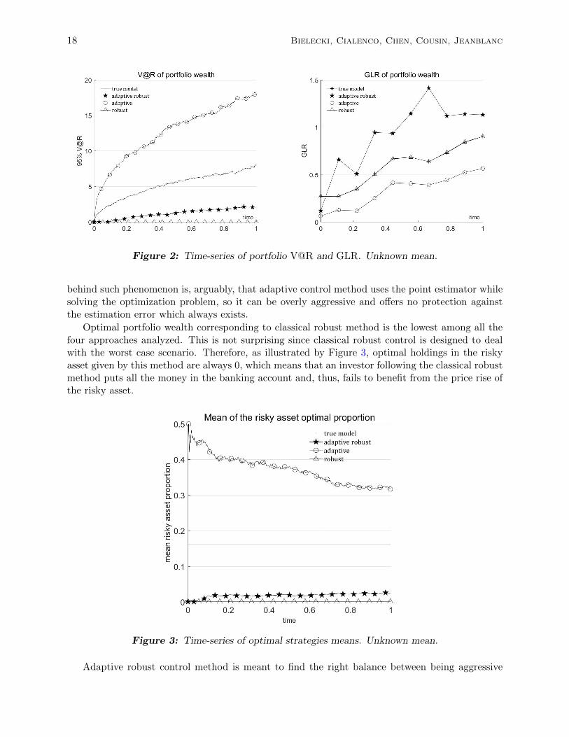
Figure 2: Time-series of portfolio V@R and GLR. Unknown mean.

behind such phenomenon is, arguably, that adaptive control method uses the point estimator whilesolving the optimization problem, so it can be overly aggressive and offers no protection againstthe estimation error which always exists.

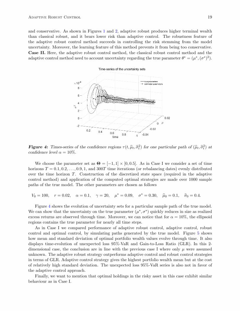
Optimal portfolio wealth corresponding to classical robust method is the lowest among all thefour approaches analyzed. This is not surprising since classical robust control is designed to dealwith the worst case scenario. Therefore, as illustrated by Figure 3, optimal holdings in the riskyasset given by this method are always 0, which means that an investor following the classical robustmethod puts all the money in the banking account and, thus, fails to benefit from the price rise ofthe risky asset.

Figure 3: Time-series of optimal strategies means. Unknown mean.

Adaptive robust control method is meant to find the right balance between being aggressive

Adaptive Robust Control 19

and conservative. As shown in Figures 1 and 2, adaptive robust produces higher terminal wealththan classical robust, and it bears lower risk than adaptive control. The robustness feature ofthe adaptive robust control method succeeds in controlling the risk stemming from the modeluncertainty. Moreover, the learning feature of this method prevents it from being too conservative.

Case II. Here, the adaptive robust control method, the classical robust control method and theadaptive control method need to account uncertainty regarding the true parameter θ∗ = (µ∗, (σ∗)2).

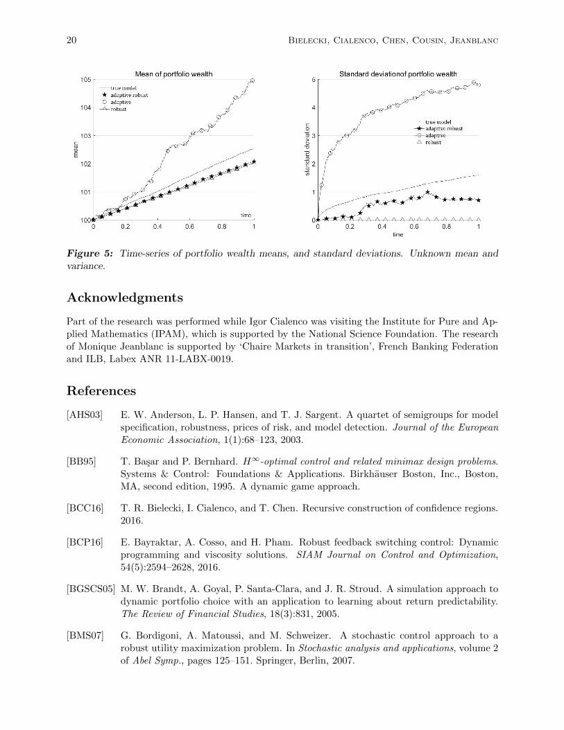
Figure 4: Times-series of the confidence regions τ(t, µt, σ2t ) for one particular path of (µt, σ

2t ) at

confidence level α = 10%.

We choose the parameter set as Θ = [−1, 1] × [0, 0.5]. As in Case I we consider a set of timehorizons T = 0.1, 0.2, . . . , 0.9, 1, and 300T time iterations (or rebalancing dates) evenly distributedover the time horizon T . Construction of the discretized state space (required in the adaptivecontrol method) and application of the computed optimal strategies are made over 1000 samplepaths of the true model. The other parameters are chosen as follows

V0 = 100, r = 0.02, α = 0.1, γ = 20, µ∗ = 0.09, σ∗ = 0.30, µ0 = 0.1, σ0 = 0.4.

Figure 4 shows the evolution of uncertainty sets for a particular sample path of the true model.We can show that the uncertainty on the true parameter (µ∗, σ∗) quickly reduces in size as realizedexcess returns are observed through time. Moreover, we can notice that for α = 10%, the ellipsoidregions contains the true parameter for nearly all time steps.

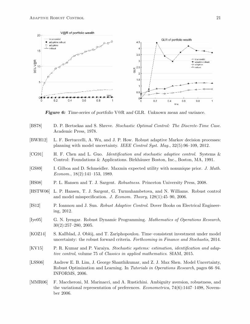
As in Case I we compared performance of adaptive robust control, adaptive control, robustcontrol and optimal control, by simulating paths generated by the true model. Figure 5 showshow mean and standard deviation of optimal portfolio wealth values evolve through time. It alsodisplays time-evolution of unexpected loss 95%-VaR and Gain-to-Loss Ratio (GLR). In this 2-dimensional case, the conclusion are in line with the previous case I where only µ were assumedunknown. The adaptive robust strategy outperforms adaptive control and robust control strategiesin terms of GLR. Adaptive control strategy gives the highest portfolio wealth mean but at the costof relatively high standard deviation. The unexpected loss 95%-VaR series is also not in favor ofthe adaptive control approach.

Finally, we want to mention that optimal holdings in the risky asset in this case exhibit similarbehaviour as in Case I.

20 Bielecki, Cialenco, Chen, Cousin, Jeanblanc

Figure 5: Time-series of portfolio wealth means, and standard deviations. Unknown mean andvariance.

Acknowledgments

Part of the research was performed while Igor Cialenco was visiting the Institute for Pure and Ap-plied Mathematics (IPAM), which is supported by the National Science Foundation. The researchof Monique Jeanblanc is supported by ‘Chaire Markets in transition’, French Banking Federationand ILB, Labex ANR 11-LABX-0019.

References

[AHS03] E. W. Anderson, L. P. Hansen, and T. J. Sargent. A quartet of semigroups for modelspecification, robustness, prices of risk, and model detection. Journal of the EuropeanEconomic Association, 1(1):68–123, 2003.

[BB95] T. Basar and P. Bernhard. H∞-optimal control and related minimax design problems.Systems & Control: Foundations & Applications. Birkhauser Boston, Inc., Boston,MA, second edition, 1995. A dynamic game approach.

[BCC16] T. R. Bielecki, I. Cialenco, and T. Chen. Recursive construction of confidence regions.2016.

[BCP16] E. Bayraktar, A. Cosso, and H. Pham. Robust feedback switching control: Dynamicprogramming and viscosity solutions. SIAM Journal on Control and Optimization,54(5):2594–2628, 2016.

[BGSCS05] M. W. Brandt, A. Goyal, P. Santa-Clara, and J. R. Stroud. A simulation approach todynamic portfolio choice with an application to learning about return predictability.The Review of Financial Studies, 18(3):831, 2005.

[BMS07] G. Bordigoni, A. Matoussi, and M. Schweizer. A stochastic control approach to arobust utility maximization problem. In Stochastic analysis and applications, volume 2of Abel Symp., pages 125–151. Springer, Berlin, 2007.

Adaptive Robust Control 21

Figure 6: Time-series of portfolio V@R and GLR. Unknown mean and variance.

[BS78] D. P. Bertsekas and S. Shreve. Stochastic Optimal Control: The Discrete-Time Case.Academic Press, 1978.

[BWH12] L. F. Bertuccelli, A. Wu, and J. P. How. Robust adaptive Markov decision processes:planning with model uncertainty. IEEE Control Syst. Mag., 32(5):96–109, 2012.

[CG91] H. F. Chen and L. Guo. Identification and stochastic adaptive control. Systems &Control: Foundations & Applications. Birkhauser Boston, Inc., Boston, MA, 1991.

[GS89] I. Gilboa and D. Schmeidler. Maxmin expected utility with nonunique prior. J. Math.Econom., 18(2):141–153, 1989.

[HS08] P. L. Hansen and T. J. Sargent. Robustness. Princeton University Press, 2008.

[HSTW06] L. P. Hansen, T. J. Sargent, G. Turmuhambetova, and N. Williams. Robust controland model misspecification. J. Econom. Theory, 128(1):45–90, 2006.

[IS12] P. Ioannou and J. Sun. Robust Adaptive Control. Dover Books on Electrical Engineer-ing, 2012.

[Iye05] G. N. Iyengar. Robust Dynamic Programming. Mathematics of Operations Research,30(2):257–280, 2005.

[KOZ14] S. Kallblad, J. Ob loj, and T. Zariphopoulou. Time–consistent investment under modeluncertainty: the robust forward criteria. Forthcoming in Finance and Stochastis, 2014.

[KV15] P. R. Kumar and P. Varaiya. Stochastic systems: estimation, identification and adap-tive control, volume 75 of Classics in applied mathematics. SIAM, 2015.

[LSS06] Andrew E. B. Lim, J. George Shanthikumar, and Z. J. Max Shen. Model Uncertainty,Robust Optimization and Learning. In Tutorials in Operations Research, pages 66–94.INFORMS, 2006.

[MMR06] F. Maccheroni, M. Marinacci, and A. Rustichini. Ambiguity aversion, robustness, andthe variational representation of preferences. Econometrica, 74(6):1447–1498, Novem-ber 2006.

22 Bielecki, Cialenco, Chen, Cousin, Jeanblanc

[PP03] G. Pages and J. Printems. Optimal quadratic quantization for numerics: the Gaussiancase. Monte Carlo Methods and Applications, 9:135–166, 2003.

[Sir14] M. Sirbu. A note on the strong formulation of stochastic control problems with modeluncertainty. Electronic Communications in Probability, 19, 2014.

[Ski03] C. Skiadas. Robust control and recursive utility. Finance Stoch., 7(4):475–489, 2003.