1

Adaptive Noise Cancelling and Time-frequency Techniques for

Rail Surface Defect Detection

B. Liang*1 S. Iwnicki1, A. Ball1 and S. Zhang2

1School of Computing and Engineering

University of Huddersfield, Huddersfield HD1 3DH, UK 2Beijing Institute of Space Launch Technology

P.O. Box 9200-71 Beijing 100076, China

*Correspondence author b.liang@hud.ac.uk

Abstract

Adaptive noise cancelling (ANC) is a technique which is very effective to remove

additive noises from the contaminated signals. It has been widely used in the fields of

telecommunication, radar and sonar signal processing. However it was seldom used for

the surveillance and diagnosis of mechanical systems before late of 1990s. As a

promising technique it has gradually been exploited for the purpose of condition

monitoring and fault diagnosis. Time-frequency analysis is another useful tool for

condition monitoring and fault diagnosis purpose as time-frequency analysis can keep

both time and frequency information simultaneously. This paper presents an ANC and

time-frequency application for railway wheel flat and rail surface defect detection. The

experimental results from a scaled roller test rig show that this approach can significantly

reduce unwanted interferences and extract the weak signals from strong background

noises. The combination of ANC and time-frequency analysis may provide us one of

useful tools for condition monitoring and fault diagnosis of railway vehicles.

Key words: adaptive noise cancelling, wheel-rail contact, time-frequency analysis, signal

processing

1. Introduction

The interest in the ability to monitor system structure integrity and detect damage at the

earliest possible stage is persistent throughout the civil, mechanical and aerospace

engineering communities. Due to the fact that many such systems are complex, dynamic

and time-varying, the necessary signal pre-processing and analysis techniques are

required in order to extract useful information from raw signals. The signal pre-

processing methods are to condition the raw signals and make every effort to eliminate

the unwanted noise from the raw signals while signal analysis techniques are to extract

signal features from the conditioned raw signals. One of the well-known techniques in

communication area for raw signal pre-processing is adaptive noise cancellation (ANC).

ANC is a technique which is very useful to remove additive noises from the contaminated

raw signals. It was firstly reported in 1975 that ANC was successfully applied to subtract

a pregnant woman’s heart rate interference from the very weak foetus heart rate

monitoring [1]. Then this technique was widely used in telecommunication, radar and

sonar signal processing because of its good performance in applications of noise

2

reduction. The results from experiments of speech enhancement and speech recognition

are especially encouraging [2-3]. After the late 1990s, ANC has also found its application

in the area of condition monitoring and fault diagnosis [4-6].

The signal analysis techniques for condition monitoring can be classified into time-

domain analysis, frequency-domain analysis, and joint time-frequency domain analysis.

The time-domain analysis methods are to identify the quantities of a signal related to its

time behaviour such as the maximum amplitude, root mean square (rms) value, kurtosis

and crest factor of a signal, while the frequency-domain analysis methods are to analyse

the contents of a signal related to its frequency behaviour, like power spectrum, cepstrum

and higher-order spectrum of a signal.[7-11]. Since machinery operating in non-

stationary mode generates a signature which at each instant of time has a distinct

frequency, it is desirable to use time-frequency analysis technique to see how frequency

changes with time. Time-frequency analysis techniques had found limited use in the past,

except for the last two decades, primarily due to their very high computational

complexity and the lack of adequate computing resources of the time. However the fast

advances of computers in the last 10 years and the outstanding potential of new time-

frequency method like wavelet transform has made them recently a very active area of

research [12-16].

Rail and wheel faults like rail surface crack, squats, corrugation, and wheel flat can cause

large dynamic contact forces at the wheel–rail interface and lead to fast deterioration of

the track. Early detection of such defects is very important for timely maintenance.

Extensive theoretical and experimental works have been carried out to investigate what is

the best way to identify rail and wheel faults. Jun et al [17] suggested a method of

estimating irregularities in railway tracks using acceleration data measured from high-

speed trains. A mixed filtering approach was proposed for stable displacement

estimation and waveband classification of the irregularities in the measured acceleration.

Kawasaki and Youcef-Toumi [18] presented a method based on the car-body acceleration

for track condition monitoring. But the car-body acceleration is highly dependent on the

primary and the secondary suspension, so the effect of the track irregularities is difficult

to extract from such data. Marija and Zili et al [19] attempted to determine a quantitative

relationship between the characteristics of the accelerations and the track defects, axle

box acceleration at a squat. The dynamic contact was simulated through finite element

modeling. Belotti et al [20] presented a method of wheel flat detection using a wavelet

transform method. In their study, a series of accelerometers were put under the rail bed to

detect the impact force caused by a wheel flat and the signals were analysed based on the

wavelet property of variable time-frequency resolution.

This paper made an attempt to use ANC technique as signal pre-processing in order to

increase the signal-to-noise ratio of a signal and also to use time-frequency analysis

techniques for time-varying impact excitation caused by rail and wheel surface defects.

The paper is presented as follows. Section 2 introduces the basic concepts for ANC and

four time-frequency analysis techniques (Short-Time-Fourier-Transform, Wigner-Ville-

Transform, Choi-Williams-Transform and Wavelet Transform). In section 3 the

3

experimental test rig is described. Experimental results and discussion are shown in

section 4. Finally conclusions are given in section 5.

2. ANC and time-frequency analysis theories

2.1. Adaptive noise cancelling technique

The principal of ANC is that it makes use of an auxiliary or reference input derived from

one or more sensors located in points in the noise or unwanted signal field where the

concerned signal is weak. The input is filtered and subtracted from a primary input

containing both signal and noise. Because the filtering and subtraction are controlled by

an appropriate adaptive process, noise reduction can be accomplished with little

distorting the signal or increasing the output noise level. Figure 1 presents the basic

philosophy of ANC. It can be seen that the primary input is a combination of the signal

source s and the noise source n. The auxiliary input is the noise source n1 which is

correlated with the primary input noise source n and is filtered to produce an estimation

of the noise source . The system output is the source estimation which is the signal s

plus noise source n, and then minus the estimation of noise source with the adaptive

filter. If n and are close enough, a better estimation of signal source can be obtained.

However there are some conditions attached for this method. The first condition is that

the signal source s is uncorrelated with noise signal n and n1. The second condition is that

in order to produce the best estimation of the signal source the ANC system output e has

to be minimized in term of least means square of power as follows [21]:

(1)

Squaring equation 1 and taking expectations in consideration of the first condition

mentioned above produces,

(2)

If the item is minimized in the least square means, the best least square

estimate of the signal can be achieved with

(3)

The least mean squares (LMS) algorithm is used for adjusting the filter coefficients to

minimize the cost function. Compared to recursive least squares (RLS) algorithms, the

LMS algorithms do not involve any matrix operations. Therefore, the LMS algorithms

require fewer computational resources and memories than the RLS algorithms. The

implementation of the LMS algorithms also is less complicated than the RLS algorithms.

To minimize the mean square error the gradient of with respect to weights w

can be set to zero. That is

=0 (4)

4

which yields the Wiener equation

(5)

Where R=E[(n1)·(n1)T] is the auxiliary inputs correlation matrix and P=E[(s+n)·(n1)] is

the cross-correlation column vector between the primary and the auxiliary inputs.

2.2. Time-frequency analysis techniques

Time-frequency analysis techniques had found limited use in the past, except for the last

two decades, primarily due to their very high computational complexity and the lack of

adequate computing resources of the time. However the fast advances of computers in the

last 10 years and the outstanding potential of new time-frequency method like wavelet

transform has made them recently a very active area of research. The most commonly

used time-frequency presentation is the Short-Time-Fourier-Transform (STFT), which

was originated from the well-known Fourier transform. In STFT time-localization can be

achieved by first windowing the signal so as to cut off only a well-localized slice of s(t)

and then taking its Fourier Transform. The STFT of a signal s(t) can be defined as [22]

(6)

Where τ and ω denote the time of spectral localization and Fourier frequency,

respectively, and h(τ-t) denotes a window function. However the STFT has some

problems with dynamic signals due to its limitations of fixed window width.

Another well-known time-frequency representation is the Wigner-Ville transform. The

Wigner transform was developed by Eugene Wigner in 1932 to study the problem of

statistical equilibrium in quantum mechanics and was first introduced in signal analysis

by the French scientist, Ville about 15 years later. It is commonly known in the signal

processing community as the Wigner-Ville Transform [23].

Signal Source

Noise Source Adaptive

Filter

System Output

+

-

s+n

n1

Primary

Input

Auxiliary

Input

Figure 1 The adaptive noise cancelling concept

=(s+n)-

5

Given a signal s(t), its Wigner-Ville transform is defined by

(7)

The Wigner-Ville transform essentially amounts to considering inner products

of copies of of the original signal shifted in time-domain with the

corresponding reversed copy . Simple geometrical considerations show

that such a procedure provides insights into the time-frequency content of a signal. From

the definition of equation (7) it can be seen that the calculation of Wigner-Ville transform

requires infinite quantity of the signal, which is impossible in practice. One practical

method is to add a window h(τ) to the signal. That leads to a new version of the Wigner-

Ville transform as follows:

(8)

Which is called pseudo-Wigner–Ville (PWV) representation.

However there is a well-known drawback of using Wigner-Ville distribution. The

interference or cross-terms exist between any two signals due to the fact the Wigner-Ville

transform is a bilinear transform. For example, if a signal consists of signal 1 and signal 2,

the Wigner-Ville transform of the signal is

) (9)

Where is called the

cross term Wigner-Ville transform of signal 1 and signal 2. In order to get rid of the

cross-term a smoothed pseudo Wigner-Ville transform (SPWVT) has to be used.

As the Wigner-Ville transform can be generalized to a large class of time-frequency

representations called Cohen’s class representations, one of natural choices is to select

some Cohen’s kernel functions which can suppress the cross-term. The Choi–Williams

Transform (CWT) is one of them. CWT was first proposed by Hyung-Ill Choi and

William J. Williams in 1989 [24]. This distribution function adopts exponential kernel to

suppress the cross-term. The CWT mathematical definition of a signal s is

(10)

The CWT can also be considered as a type of “smoothed WVT” due to the fact that as

seen in equation (10) if →+ CW will become WVT. On the other hand, the smaller

is, the better the cross-term reduction is. However, the kernel gain does not decrease

along the axes in the ambiguity domain. Consequently, the kernel function of the CWT

function can only filter out the cross-terms result from the components differ in both time

and frequency centre. Despite this disadvantage, CWT still is one of the most popular

time-frequency analysis techniques.

6

Finally another relatively new time-frequency analysis technique is the wavelet transform

(WT). Unlike Fourier analysis which breaks up a signal into sine waves of various

frequencies wavelet analysis is to decompose a signal into shifted and scaled versions of

the original (or mother) wavelet. One major advantage provided by wavelets is the ability

to perform local analysis. Because wavelets are localized in time and scale, wavelet

coefficients are able to localize abrupt changes in smooth signals. Also the WT is good at

extracting information from both time and frequency domains. However the WT is

sensitive to noise.

For a signal s(t), the WT transform can be given as [25]

(11)

Where ψ(t-τ/x) is the mother wavelet with a dilation x and a translation τ which is used

for localization in frequency and time.

3. The roller test rig and experiments set up

In order to validate the suggested techniques, a series of experiments has been carried out

on one 1/5 scale roller rig at University of Huddersfield. A scaled roller rig can offer a

number of advantages over a full size roller rig such as a smaller space occupied by the

rig and more easily handled. A scaled roller rig can be used to demonstrate the behaviour

of a bogie vehicle under various running conditions without losing generality as long as

the effect of scaling on the equations of governing the wheel-rail interaction (creep force)

is maintained. Our roller rig scaling factor for the mass is 53 and the inertia scaling factor

is 55 which were set according to Kalker’s theory. The roller rig consists of four rollers

supported in yoke plates incorporating the rollers in supporting bearings. The roller

motion is provided by servo hydraulic actuators which are connected directly to the

supporting yoke plates, these actuators being controlled by a digital controller which

allows the inputs to follow defined waveforms or measured track data. The bogie vehicle

parameters were selected to represent those of a typical high speed passenger coach (the

BR Mk4 passenger coach). The wheel profile is a machined scale version of the BR P8

profile and the rollers have a scale BS 110 rail profile with no rail inclination.. The

parameters for the roller rig are given in Table 1. As indicated in Figure 1 two

accelerometers were installed on wheel axle boxes. One dent with a surface size of 3mm

long x 2mm wide x 0.2mm deep was made on the surface of one rollers to simulate rail

surface defect. One wheel flat with a size of 2mm wide x 1mm long was also made on the

wheel paired with the dented roller. The accelerometer with the underneath roller defect

was used as the primary input of the ANC filter and another accelerometer without

underneath roller defect was linked to the auxiliary input of the ANC filter as indicated in

Figure 1-2. The acceleration data were sampled by a YE6231 data acquisition system

which has 4 channels, 24-bit resolution and maximum sampling rate 100 kHz.

Table 1 The parameters for the roller rig

Parameter Full size 1/5 scale

wheelset mass 1850 kg 14.8 kg

7

wheelset rotational inertia 174 kgm2 0.056 kgm2

wheelset roll/yaw inertia 935 kgm2 0.300 kgm2

bogie mass 2469 kg 19.75 kg

bogie roll inertia 1130 kgm2 0.361 kgm2

bogie yaw inertia 2142 kgm2 0.685 kgm2

wheel diameter 0.914 m 0.182 m

gauge 1.435 m 0.287 m

wheelbase 2.5 m 0.5 m

speed v v/5

Figure 1 The primary and auxiliary inputs of the ANC filter

Figure 2 The photo of the 1/5 roller test rig

4. Experimental results and discussions

Output Primary input

Auxiliary input

ANC

Roller surface defect

Bogie

frame Rollers Wheelset

Accelerometers

8

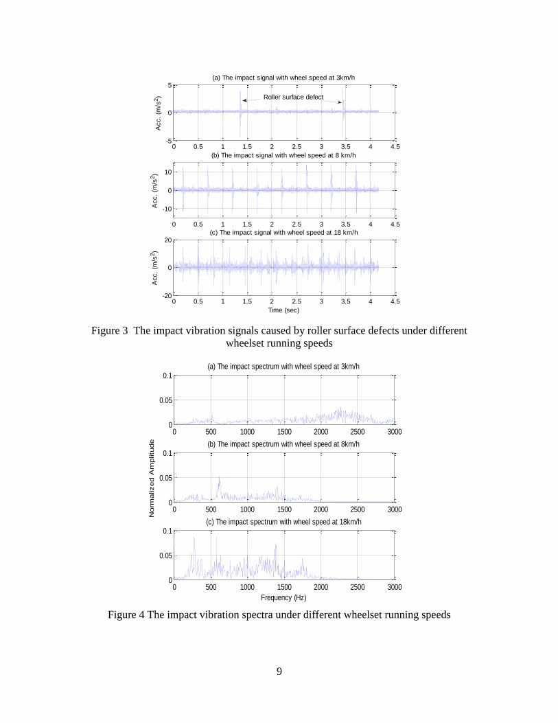
In figure 3, a series of impact vibration pulses caused by a roller surface defect under

three different wheelset running speeds are presented. When the wheelset running speed

is low, the clear impact pulses caused by the roller surface defect can be seen ( figure

4(a)). However as the wheelset running speed rises, the roller surface defect impact

pulses will be contaminated by wheel flange contact and some other unknown noises as

shown in figure 4(c). Some kinds of signal processing techniques are necessary in order

to eliminate the unwanted noises. Figure 4 presents the corresponding spectra of the

impact vibration under different wheelset running speeds. It shows that when wheelset

speed is low, the impact caused by the defect can only excite some higher frequency

content of the wheelset system (between 2000-2500Hz ). As the wheelset speed continues

to rise as indicated in figure 4(b)-(c), the higher frequency caused by the impact

diminished and the lower band natural frequencies 300-400Hz, 600-650Hz and 1100-

1300Hz became the dominant frequencies in the spectrum because the creep forces

between wheel and rail were increased with the wheelset rotating speed rising.

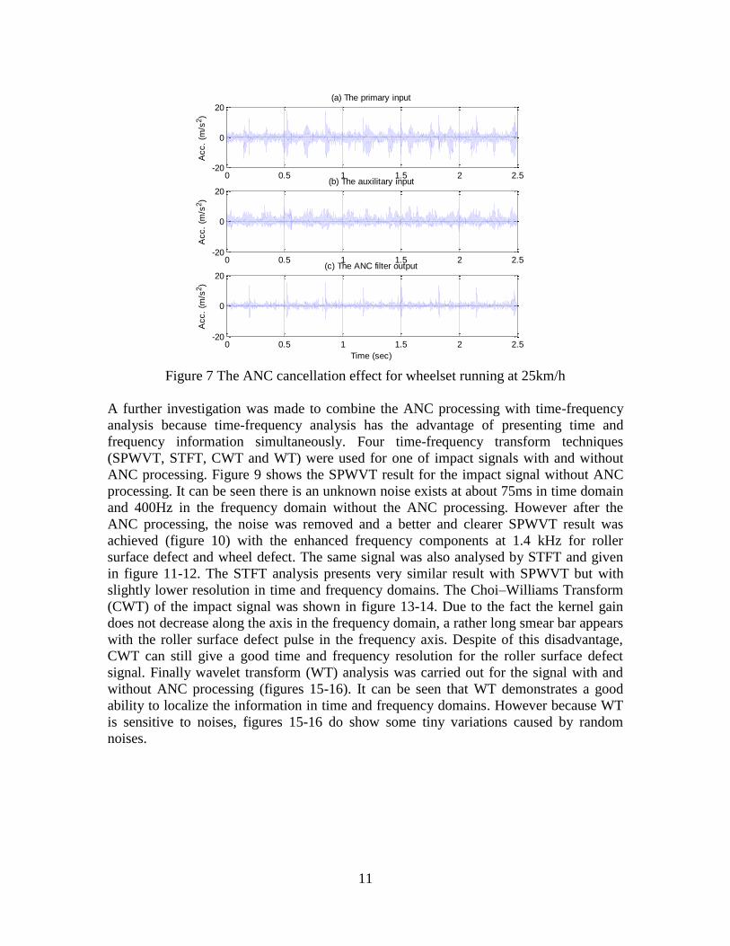
Figures 6-8 present some results which show the effects of the ANC noise cancellation

for the wheelset running from low to high speeds. Figure 6(a) is the vibration signal of

the roller with a surface defect used as the primary input for the ANC filter (the top wheel

of the right wheelset) and figure 6(b) is the vibration signal of the roller without a surface

defect used as auxiliary input for the ANC filter (the bottom wheel of the right wheelset),

and figure 6(c) is the signal after ANC processing. The slight signal to noise ratio

improvement can be seen with and without ANC processing in figure 6. Figure 7 gives

the ANC effect for wheelset running speed 15km/h. As expected the impact vibration

amplitude is increased proportionally with the wheelset speed and a better ANC

cancellation performance is observable in figure 7. When the wheelset running speed

continues to rise, the impact signal caused by roller surface defect is severely corrupted

by some unwanted noises like the wheelset lateral movement and the contact between

wheel flanges and rollers (figure 8(a)). However the ANC processing can still recover the

corrupted impact signal well as demonstrated in figure 8(c) despite there is a low signal-

to-noise ratio when compared with the low wheelset running speed.

9

0 0.5 1 1.5 2 2.5 3 3.5 4 4.5-20

0

20

Time (sec)

Acc.

(m/s

2)

(c) The impact signal with wheel speed at 18 km/h

0 0.5 1 1.5 2 2.5 3 3.5 4 4.5

-10

0

10

Acc.

(m/s

2)

(b) The impact signal with wheel speed at 8 km/h

0 0.5 1 1.5 2 2.5 3 3.5 4 4.5-5

0

5

Acc.

(m/s

2)

(a) The impact signal with wheel speed at 3km/h

Roller surface defect

Figure 3 The impact vibration signals caused by roller surface defects under different

wheelset running speeds

0 500 1000 1500 2000 2500 30000

0.05

0.1(a) The impact spectrum with wheel speed at 3km/h

0 500 1000 1500 2000 2500 30000

0.05

0.1

Norm

alized A

mplitu

de (b) The impact spectrum with wheel speed at 8km/h

0 500 1000 1500 2000 2500 30000

0.05

0.1

Frequency (Hz)

(c) The impact spectrum with wheel speed at 18km/h

Figure 4 The impact vibration spectra under different wheelset running speeds

10

0 1 2 3 4-5

0

5A

CC

.(m

/s2)

(b) The auxilitary input0 1 2 3 4

-5

0

5(a) The primary input

0 1 2 3 4-5

0

5

Time (sec)

(c) The ANC filter input

Figure 5 The ANC cancellation effect for wheelset running at 3km/h

0 0.5 1 1.5 2 2.5

-10

0

10

Time (sec)

Acc.

(m/s

2)

(c) The ANC filter output

0 0.5 1 1.5 2 2.5

-10

0

10

Acc.

(m/s

2)

(b) The auxilitary input

0 0.5 1 1.5 2 2.5

-10

0

10

Acc.

(m/s

2)

(a) The primary input

Figure 6 The ANC cancellation effect for wheelset running at 15km/h

11

0 0.5 1 1.5 2 2.5-20

0

20

Acc.

(m/s

2)

(a) The primary input

0 0.5 1 1.5 2 2.5-20

0

20A

cc.

(m/s

2)

(b) The auxilitary input

0 0.5 1 1.5 2 2.5-20

0

20

Time (sec)

Acc.

(m/s

2)

(c) The ANC filter output

Figure 7 The ANC cancellation effect for wheelset running at 25km/h

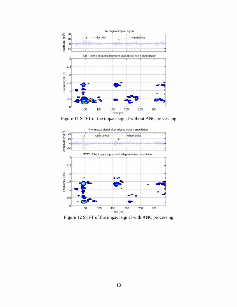
A further investigation was made to combine the ANC processing with time-frequency

analysis because time-frequency analysis has the advantage of presenting time and

frequency information simultaneously. Four time-frequency transform techniques

(SPWVT, STFT, CWT and WT) were used for one of impact signals with and without

ANC processing. Figure 9 shows the SPWVT result for the impact signal without ANC

processing. It can be seen there is an unknown noise exists at about 75ms in time domain

and 400Hz in the frequency domain without the ANC processing. However after the

ANC processing, the noise was removed and a better and clearer SPWVT result was

achieved (figure 10) with the enhanced frequency components at 1.4 kHz for roller

surface defect and wheel defect. The same signal was also analysed by STFT and given

in figure 11-12. The STFT analysis presents very similar result with SPWVT but with

slightly lower resolution in time and frequency domains. The Choi–Williams Transform

(CWT) of the impact signal was shown in figure 13-14. Due to the fact the kernel gain

does not decrease along the axis in the frequency domain, a rather long smear bar appears

with the roller surface defect pulse in the frequency axis. Despite of this disadvantage,

CWT can still give a good time and frequency resolution for the roller surface defect

signal. Finally wavelet transform (WT) analysis was carried out for the signal with and

without ANC processing (figures 15-16). It can be seen that WT demonstrates a good

ability to localize the information in time and frequency domains. However because WT

is sensitive to noises, figures 15-16 do show some tiny variations caused by random

noises.

12

-10

0

10

20

Am

plit

ude (

m/s

2)

The original impact signal

SPWVT of the impact signal without adaptive noise cancellation

Time [ms]

Fre

quency [

kH

z]

50 100 150 200 250 3000

0.5

1

1.5

2

2.5

3

roller defect wheel defect

Figure 9 SPWVT of the impact signal without ANC processing

-10

0

10

20

Am

plit

ude (

m/s

2)

The impact signal after adaptive noise cancellation

SPWVT of the impact signal with adaptive noise cancellation

Time [ms]

Fre

quency [

kH

z]

50 100 150 200 250 3000

0.5

1

1.5

2

2.5

3

roller defect wheel defect

Figure 10 SPWVT of the impact signal with ANC processing

13

-10

0

10

20

Am

plit

ud

e(m

/s2)

The original impact signal

STFT of the impact signal without adaptive noise cancellation

Time [ms]

Fre

qu

en

cy

[kH

z]

50 100 150 200 250 3000

0.5

1

1.5

2

2.5

3

wheel defectroller defect

Figure 11 STFT of the impact signal without ANC processing

-10

0

10

20

Am

plit

ude (

m/s

2)

The impact signal after adptive noise cancellation

STFT of the impact signal with adaptive noise cancellation

Time [ms]

Fre

quency [

kH

z]

50 100 150 200 250 3000

0.5

1

1.5

2

2.5

3

wheel defectroller defect

Figure 12 STFT of the impact signal with ANC processing

14

-10

0

10

20

Am

plit

ude (

m/s

2)

The original impact signal

CWT of the impact signal without adaptive noise cancellation

Time [ms]

Fre

quency [

kH

z]

50 100 150 200 250 3000

0.5

1

1.5

2

2.5

3

roller defect wheel defect

Figure 13 CWT of the impact signal without ANC processing

-10

0

10

20

Am

plit

ude (

m/s

2)

The impact signal after adaptive noise cancellation

CWT of the impact signal with adaptive noise cancellation

Time [ms]

Fre

quency [

kH

z]

50 100 150 200 250 3000

0.5

1

1.5

2

2.5

3

roller defect wheel defect

Figure 14 CWT of the impact signal with ANC processing

15

-10

0

10

20

Am

plitu

de

(m

/s2) The original impact signal

Time (ms)

Fre

qu

en

cy

(Hz)

WT of the impact signal without adaptive noise cancellation

0 50 100 150 200 250 3000

500

1000

1500

2000

2500

roller defect wheel defect

Figure 15 WT of the impact signal without ANC processing

-10

0

10

20

Am

plitu

de

(m

/s2) The impact signal after adaptive noise cancellation

Time (ms)

Fre

qu

en

cy

(Hz)

WT of the impact signal with adaptive noise cancellation

0 50 100 150 200 250 3000

500

1000

1500

2000

2500

roller defect wheel defect

Figure 16 WT of the impact signal with ANC processing

5. Conclusions

In this study, an adaptive noise cancelling (ANC) technique with time-frequency signal

processing was proposed to detect rail surface defects. A series of experiments was

carried out on a 1/5 scale roller test rig. The experiment results demonstrated that if a

wheelset is running at low speed the ANC method is less attractive because of the good

original signal-to-noise ratio in the vibration signal. However if a wheelset is running at

relatively high speed, there is a significant level of noise presented. For example, the

wheel flange contacts between wheel and rail can contaminate the wanted signal caused

by rail surface defects and makes the detection difficult. The experiments proved that

ANC could be an effective way to eliminate this unwanted noise.

16

Further investigation about time-frequency analysis techniques was also made for rail

surface defects. Four time-frequency analysis methods (STFT, SPWVT, CWT and WT)

were tested. The results show all four time-frequency methods can present proper time-

frequency information for the vibration generated by wheel flat and rail surface defects.

However they have different advantages and disadvantages. The SPWVT gives a better

representation with a both time and frequency resolutions while WT shows good

localisations in both time and frequency dimensions. STFT presents slightly lower

resolutions in time and frequency axes. CWT displays reasonable information of the

roller surface defect signal in time and frequency domains but with some smear

disadvantage effects in frequency domain caused by its inherited problem. Despite of

this drawback CWT is still a good alternate choice for the time-frequency analysis. The

combination of the ANC technique and an appropriate time-frequency analysis method

like SPWVT and WT may provide a very useful tool for condition monitoring and fault

diagnosis in the railway industry.

References

1. Bernard, W.J. etc Adaptive noise cancelling: principles and applications,

Proceedings of the IEEE, Vol.63, No.12, December. 1975, pp1672-1716

2. Van Compernolle, D. etc, Speech recognition in noisy environment with the aid

of microphone arrays, Proceedings of the Eurospeech, Paris, France, 1989, pp657-

666

3. Shields, P.W. and Campell, D.R. Speech enhancement using a multi-microphone

sub-band adaptive noise canceller, Proceedings of Eurospeech, Budapest,

Hungary, 1999, pp2559-2566

4. Shao, Y. and Nezu, K. Detection of self aligning roller bearing fault using

asynchronous adaptive noise cancelling technology, JSME International Journal,

Series, Vol.42 (1), 1999, pp33-43

5. Randall, R.B., Bearing diagnosis in helicopter gearboxes, Proceedings of the 14th

International Congress, Vol.1, UK 2001, pp434-453

6. Ayala, Botto, M. etc, Intelligent active noise control applied to a laboratory

railway coach model, Control Engineering Practice, Vol.13, Issue 4, 2005, pp473-

484

7. I. Yesilyurt, Fault detection and location in gears by the smoothed instantaneous

power spectrum distribution, NDT & E International, Volume 36, Issue 7,

October 2003

8. Peng Chen, Masatoshi Taniguchi, Toshio Toyota, Zhengja He, Fault diagnosis

method for machinery in unsteady operating condition by instantaneous power

spectrum and genetic programming, Mechanical Systems and Signal Processing,

Volume 19, Issue 1, 2005

9. R.B. Randall, Cepstrum analysis, Encyclopedia of Vibration, 2001

10. B. Liang, S. Iwnicki and Y. Zhao, Application of power spectrum, cepstrum,

higher order spectrum and neural network analyses for induction motor fault

diagnosis, Mechanical Systems and Signal Processing, Vol.39, Issue 4, 2013

17

11. L. Saidi, F. Fnaiech, H. Henao, G-A. Capolino, G. Cirrincione, Diagnosis of

broken-bars fault in induction machines using higher order spectral analysis, ISA

Transactions, Volume 52, Issue 1, 2013

12. Zhipeng Feng, Ming Liang, Fulei Chu, Recent advances in time–frequency

analysis methods for machinery fault diagnosis: A review with application

examples, Mechanical Systems and Signal Processing, Volume 38, Issue 1, 2013

13. N. Baydar and A. Ball, A comparative study of acoustic and vibration signals in

detection of gear failure using Wigner-Ville distribution, Mechanical Systems and

Signal Processing, Vol.15, 2001

14. V.V. Polyshchuk, F. K. Choy and M. J. Braun, Gear fault detection with Time-

frequency based parameter NP4, International Journal of Rotating Machinery,

Vol.8, No. 1, 2002

15. Ervin Sejdić, Igor Djurović, Jin Jiang, Time–frequency feature representation

using energy concentration: An overview of recent advances, Digital Signal

Processing, Volume 19, Issue 1, 2009

16. N. Saravanan, K.I. Ramachandran, Incipient gear box fault diagnosis using

discrete wavelet transform (DWT) for feature extraction and classification using

artificial neural network (ANN), Expert Systems with Applications, Volume 37,

Issue 6, 2010

17. Jun Seok Lee, Sunghoon Choi, et al, A mixed filtering approach for track condition

monitoring using accelerometers on the axle box and bogie, IEEE Transactions on

Instrumentation and Measurement, Vol.61, No.3, March, 2012

18. J. Kawasaki and K. Youcef-Toumi, Estimation of rail irregularities, Proceedings

American Control Conference., Anchorage, USA, May 2002

19. Marija Molodova, Zili Li and Rolf Dollevoet, Axle box acceleration:

Measurement and simulation for detection of short track defects, Wear, Vol.271,

No.3, 2011

20. V. Belotti, F. Crenna, R. C. Michelini, and G. B. Rossi, Wheel-flat diagnostic tool

via wavelet transform, Mechanical Systems and Signal Processing Vol. 20, No.2,

2006

21. Wiener, N. Extrapolation, interpolation and smoothing of stationary time series

with engineering applications, New York, Wiley, 1949

22. Hlawatsch, F. and Auger, F. Time-frequency analysis, John Wiley & Sons Inc,

USA 2005

23. Qian, S. Introduction to time-frequency and wavelet transforms, Prentice Hall,

London, 2002

24. Sardy, S. and Tseng, P. Robust wavelet de-noising, IEEE Trans. of Signal

Processing, Vol.49 (6), 2001

25. Hamid, A. T. and Karim, M.M.R, Rail defect diagnosis using wavelet packet

decomposition, IEEE Trans. of Industry Applications, Vol.39, No.5, Sept. 2003