Adaptive Learning Models of Consumer Behavior

Ed Hopkins∗

Edinburgh School of EconomicsUniversity of EdinburghEdinburgh EH8 9JY, UK

January, 2006

Abstract

In a model of dynamic duopoly, optimal price policies are characterized as-suming consumers learn adaptively about the relative quality of the two products.A contrast is made between belief-based and reinforcement learning. Under re-inforcement learning, consumers can become locked into the habit of purchasinginferior goods. Such lock-in permits the existence of multiple history-dependentasymmetric steady states in which one firm dominates. In contrast, belief-basedlearning rules must lead asymptotically to correct beliefs about the relative qualityof the two brands and so in this case there is a unique steady state.

Journal of Economic Literature classification numbers: C73, D11, D83, L13, M31.

Keywords: learning, consumer behavior, dynamic pricing, behavioral economics,reinforcement learning, market structure.

∗I would like to thank Andreas Blume, Pradeep Chintagunta, John Duffy, Teck Ho, Josef Hofbauer,Tatiana Kornienko, Al Roth, Karl Schlag and Jonathan Thomas for helpful discussions. I acknowledgesupport from the Economic and Social Research Council, award reference RES-000-27-0065. Errorsremain my own. E.Hopkins@ed.ac.uk, http://homepages.ed.ac.uk/ehk

1 Introduction

Adaptive learning models attempt to describe the behavior of agents faced with re-peated decision problems by assuming they use simple learning rules. These modelsare used in a number of apparently disparate environments. Economic theorists haveanalyzed them in abstract settings.1 They have been fitted to actual choice data bothin economic experiments and the quite different context of the empirical analysis ofconsumer behavior.2 Despite differences in aims and terminology, some models of dy-namic choice found in empirical marketing analysis are essentially the same as thoseused in economic theory. This research in marketing supports the experimental evidencethat even simple adaptive learning models can help to explain human behavior. In thecontext of econometric work on experimental data, there has been an active debate aswhether the more sophisticated belief-based models or very simple reinforcement learn-ing models offer the better fit. Up to now, this has been of interest because it throwslight upon human reasoning processes. However, if the same question is consideredin the context of consumer choice, there may be significant practical implications toconsider as well.

This paper investigates the hypothesis that whether consumer behavior is best de-scribed by belief-based or reinforcement learning may have a significant impact onmarket organization. In particular, we examine a model of dynamic duopoly, whereconsumers learn about the relative quality of the two different brands. The productis an experience good and so information is partial: consumers only learn the payoffto the good they actually consume. First, we investigate a reinforcement type learn-ing model, where more familiar products have a greater probability of being selected.Consequently, consumers can become locked into inferior choices. Such lock-in per-mits the existence of multiple history-dependent steady states. When multiple steadystates exist, even if the two firms are identical in terms of costs and product quality,the symmetric outcome is unstable: one firm must dominate. This outcome under re-inforcement learning is then contrasted with the outcome under belief-based learning.This form of learning leads to correct beliefs about relative quality even under partialinformation. Firms can influence consumer opinion only in the short run: if consumers’initial estimate of a firm’s quality is high (low), it has an incentive to charge above(below) the myopic price in order to slow (speed up) learning. Given the convergence ofbeliefs to the unique correct outcome, the firms must converge to a unique steady state,where prices are the same as under complete information. This paper, therefore, showsthat the small differences in the learning rules, between belief-based and reinforcementlearning, can have dramatic effects on market outcomes.

1Theoretical papers in this field include Arthur (1993), Rustichini (1999), Börgers and Sarin (2000),Sarin and Vahid (1999), Börgers et al. (2004). A survey of the use of adaptive learning models ingames can be found in Fudenberg and Levine (1998).

2Empirical work includes Erev and Roth (1998), Camerer and Ho (1999), Erev and Barron (2001)and Blume et al. (2002). Examples of work in marketing are Chintagunta and Rao (1996), Seetharamanand Chintagunta (1998), Ho and Chong (2003).

1

The situation to be modelled can be thought of as a consumer going on a regularbasis to a supermarket to buy a grocery item and choosing between two competingbrands. This type of decision has several aspects which I would like to emphasize. First,the prices for the competing brands are usually clearly marked on the shelves. Thus,the learning the consumer has to undertake is not about prices or their distribution.However, the goods in question are typically experience goods. One has to take themhome and consume them before their quality is known. Second, quality in this contextis very often subjective and imprecise, for example, whether a food product tastesgood. Third, because each successive purchase decision is relatively unimportant toan individual consumer, a model of boundedly-rational behavior may explain actualchoices well. Such boundedly-rational agents may have a impression of quality that isambiguous and difficult to measure against past experience. As a consequence, it maybe very difficult to be confident about relative quality. For example, I think I like thebrand I bought today, but is it clearly better than the one I bought last month? Indeed,in this paper it is assumed that the consumption experience is noisy and memory isimperfect.

The formal model of price competition analyzed here is derived from that of Chin-tagunta and Rao (1996), who similarly consider a dynamic duopoly with adaptive con-sumers. Their work is quite distinctive from most of the literature in economics onlearning. First, there is the mixture of rational behavior by sellers and reinforcementlearning by boundedly rational buyers. Second, while the recent literature on adaptivelearning has largely focussed on abstract exogenous environments, Chintagunta andRao’s work is also empirical. The model is fitted to data on actual prices, sales andconsumer purchases. They find, for example, that a dynamic specification, taking intoaccount consumers’ past purchases, outperforms a static logit model. This result, as Iargue in Section 7 of this paper, provides some support for the hypothesis that learningis in fact suboptimal.

Nonetheless, the difference between this current paper and the work of Chintaguntaand Rao (1996) is large, and reflects the difference between economics and marketingscience. First, the principal question here is one of welfare: do consumers learn to makecorrect choices and what is the implication that has for the competitiveness of theresulting market structure. In contrast, Chintagunta and Rao’s (1996) main objective,as with much marketing analysis, is to predict consumer choice. Second, Chintaguntaand Rao do not investigate whether the reinforcement learning rule they specify wouldlead a consumer to choose the brand which she would prefer in the case of perfectinformation. We show that frequently this will not be the case. Third, Chintaguntaand Rao, in characterizing the dynamic pricing equilibrium, did not identify, as is donehere, that there may be multiple steady states. Finally, in their paper only one learningrule is considered. Here, the results under reinforcement learning are contrasted withthose resulting under belief based learning, thereby demonstrating that it is familiaritybased learning that is responsible for the pathological outcome, and not the situationof experience goods in itself.

2

This latter point is also what differentiates the current work from an earlier litera-ture, Schmalensee (1978) and Smallwood and Conlisk (1979), that concentrates exclu-sively on simple forms of reinforcement learning. In these models also, consumers donot necessarily learn which is the highest quality brand. The contribution here is toclarify the conditions on the form of consumer learning under which this is possible.Furthermore, in the last few years, the analysis of experimental data has shown theeffectiveness of adaptive learning models in predicting subject behavior. This, com-bined with the empirical marketing work of Chintagunta and Rao (1996) and Ho andChong (2003), offers the intriguing prospect of estimating consumer learning modelswith actual consumer choices. Given the theoretical differences between reinforcementand belief-based learning, in Section 7, I offer two empirical tests that potentially coulddistinguish between the two models.

The focus on bounded rationality differentiates this paper from most previous litera-ture on dynamic pricing of experience goods that has assumed fully rational consumers.3

One strand of the existing literature is based on the quality of the good being privateinformation to the seller. The consumer then learns about product quality by makinghighly sophisticated inferences from the resulting strategic behavior of firms. Depend-ing on the model and/or the parameters of a single model, a seller can signal that thequality of her good is higher than the alternative by charging a price that is eitherhigher or lower than the price that would be myopically optimal (Milgrom and Roberts(1986); Bagwell and Riordan (1991)). Here, consumers can only learn if a brand isof high quality through repeated consumption experience. Bergemann and Välikmäki(1996) is much closer in that it examines the effect of strategic pricing on the rate ofinformation acquisition by a buyer. However, it is quite different in that the buyer’s be-havior is given by the solution to a stochastic dynamic optimization problem, allowingfor an optimal level of experimentation.

Strategic and adaptive models may well be complementary, with different modelsdoing better in different circumstances. For example, Bergemann and Välikmäki (1996),to motivate their model of optimal learning, give the example of a factory managerchoosing which production technology to buy. Indeed, such professional decision-makersfaced with sharp incentives may well be well-described by optimal learning models.Adaptive models, on the other hand, may do well in those consumer markets where asingle purchase represents very small stakes. Indeed, this paper is not the first to applylearning models to consumer behaviour. Weisbuch, Kirman and Herreiner (2000) andKirman and Vriend (2001), in work that is very close to the present approach, analyzeadaptive learning models of consumer behavior and similarly examine conditions underwhich consumers become loyal to one seller. The principal difference is that here firmsare forward looking and price dynamically. Erev and Haruvy (2001) also considerthe implications of adaptive learning by consumers but again firms have fixed pricingpolicies.4 Ellison and Fudenberg (1995) look at social learning, where agents learn from

3Belief-based adaptive learning, although more sophisticated than reinforcement learning is stillsome way short of full rationality in the traditional sense.

4Other work on adaptive learning has had adaptive learning by sellers as well as by buyers (Hopkins

3

the experience of others as well as from their own. Certainly researchers in consumerbehavior have found it plausible that consumers may be prone to a number of cognitivebiases, see for example Erdem et al. (1999). One which seems particular relevantin this context is “confirmatory bias”. As Rabin and Schrag (1999) discover, thereis substantial psychological evidence that once individuals form a hypothesis, they paygreater attention to subsequent evidence that supports that hypothesis than to evidencethat is non-supportive. In the current context, this would suggest that consumers maybe relatively unwilling to switch away from a favored brand.

This paper highlights a source of bias that is even more basic, but which has sig-nificant implications for market organization. Imagine a consumer who initially hasgreater goodwill towards brand X than the rival brand Y. So, all other factors beingequal, she will mostly purchase X, and only rarely sample Y. Now, suppose her choicedecision is based on beliefs: estimates of the relative quality of the two brands. Then,the low frequency of purchase of Y will not matter in the long run, as eventually shewill accumulate a sufficient number of observations to gain a clear picture of the averagequality of Y, and if this is higher than that of X, she will switch allegiance. In contrast,suppose a consumer chooses on the basis of familiarity, a stock of goodwill. Then, inthe intervening time between purchases of Y, when he is consuming X, that stock ofgoodwill towards Y diminishes, he forgets about it. The probability of buying Y falls.He may then never accumulate sufficient positive experience to realize that in fact Yis just as good, or even superior. That is, quite subtle difference in mental attitudetoward choices not made, products not consumed, can have quite profound effects onlong run outcomes.

The result is that, when consumers are reinforcement learners, possession of a highinitial market share is self-reinforcing. There is an extensive literature in industrialorganization concerned with the origins of market dominance. Recent theoretical ex-planations for sustained dominance include network effects, increasing returns to scaleand learning by doing. Here none of these factors are present but there is still lock-in.This, however, is broadly consistent with the empirical findings of Sutton (1991) on in-dustries in the food sector, where some outcomes seem history dependent in industries,without network externalities, but where consumer tastes, loyalty and perceptions ofquality are important.

In examining dynamic oligopoly, there is the question of which equilibrium conceptto use. Open loop equilibrium, as used by Chintagunta and Rao (1996), earlier bySchmalensee (1978) and more recently, for example, by Cellini and Lambertini (1998),has the advantage of analytic simplicity. It is true that many researchers in industrialorganization prefer Markov perfect/closed loop equilibrium, despite the fact that, exceptin simple linear-quadratic models, its complexity precludes analysis except by numericalmethods. In contrast, the open loop equilibrium can be analyzed qualitatively, revealingmuch information such as the number of steady states and their stability. Furthermore,the known disadvantages of open loop equilibria, that it in effect allows commitment to

and Seymour (2002); Harrington and Chen (2003)).

4

a complete strategy path, are limited here as firms compete on price not quantity. Thatis, the fact that the open loop equilibrium in the model analysed here has asymmetricsteady states cannot be attributed to a Stackleberg phenomenon, where one firm obtainsdominance simply by committing to a high level of output. Finally, Markov perfectequilibrium is useful for the analysis of how firms respond to stochastic realisations ofdemand or other variables. But in the current model, while the evolution of individualconsumer behaviour is stochastic, there are no aggregate shocks. So, it is possiblethat a deterministic approximation, averaging over a large number of consumers, cancapture the essentials of consumer behaviour. In turn, open loop equilibrium may be areasonable approach. This is discussed further in Section 6.

2 Adaptive Learning, Hypothetical Reasoning andSuboptimal Learning

This section introduces the models of adaptive learning used in this analysis and reviewsthe evidence as to whether adaptive learning can lead to optimal choices. A crucialaspect will be how capable an agent is of hypothetical reasoning, in particular, how shetreats the question, “How well would I have done, if I had chosen differently from thechoice I actually made?” This matters, as in many choice situations, including that ofexperience goods, one only sees the payoff to the choice actually consumed, leaving oneto speculate if one could have done better by having chosen differently. The danger isthat since the value of unchosen alternative is less clear, one will become convinced thatone’s own choice is superior, simply because it was the one chosen, not because of anyobjective superiority. As we will see, there is both theoretical and empirical evidencethat this can be an important phenomenon.

Models of learning have been employed both to explain behavior in games and insingle person decision making. There is now considerable evidence that they can ex-plain actual choice behavior (Erev and Roth, 1998; Camerer and Ho, 1999; Erev andBarron, 2001). In games, payoffs are determined by the choices of one’s opponentsand in decision problems, by an exogenous random process, but in both cases, learn-ing rules have three components. First, a decision maker is endowed with propensities(alternative terms are assessments or weights or scores), one for each of the possibleactions in her action set. The propensities of a representative agent we denote asθ = (θ1, θ2, ..., θn) ∈ IRn, when the agent must choose from n actions. Second, there is achoice rule that chooses an action as a function of current propensities. A general prin-ciple is that actions with higher propensities are chosen with higher probability. Finally,there is an updating rule, which changes the propensities in response to experience.

The choice rule that has attracted the most attention is the logit or exponential rule

xi(t) =exp(βθi(t))Pnj=1 exp(βθj(t))

. (1)

5

where xi(t) is the probability that the agent chooses action i at time t. In the exponentialchoice rule, the parameter β represents the degree of optimization. At high levels of βthe agent will choose the action with the highest propensity with very high probability.

There have been two commonly used differing assumptions about what informationis available when updating propensities. If an agent in each period can observe thereturn to all possible actions, including the “foregone” payoffs to actions that were nottaken, this is “full” information in the terminology of Rustichini (1999). If, however, theagent can only see the payoff to the action actually taken this is “partial” information.A crucial assumption here is that a consumer choosing amongst experience goods is ina situation of partial information: she only finds out about the good that she actuallychooses. Therefore, we look at adaptive learning models that only use informationabout actual payoffs.

The payoff that an agent receives at any given time will be random in two senses.First, this is because given a choice rule such as the logit above, the action she chooseswill be random. Second, in addition, it is assumed that experience is stochastic. Specif-ically, if at time t, conditional on taking the action i an agent receives a payoff ui(t)which is a random variable with mean ui.

Our first updating rule can be called reinforcement learning. Upon receiving apayoff, the agent then updates his propensities

θi(t+ 1) = (1− δ)θi(t) + δui(t)θj(t+ 1) = (1− δ)θj(t), for all j 6= i

(2)

where 1 ≥ δ > 0 is a “recency” parameter. If δ is equal to one, then only the verylast experience is remembered. With δ close to zero, experience from long ago may stillhave a significant weight in current beliefs. Crucially, this rule responds only to realizedpayoffs. No information about payoffs to actions not taken is utilized. This assumptionis found in the reinforcement learning models put forward by Arthur (1993) and Erevand Roth (1998). This may be because the payoff to other actions at that time was notobserved, there is partial information, or the learner is boundedly rational. Anothermodel that uses only partial information has recently been proposed by Sarin and Vahid(1999).5 The rule is, if action/good i is chosen at time t, then

θi(t+ 1) = (1− δ)θi(t) + δui(t)θj(t+ 1) = θj(t) for all j 6= i.

(3)

Note that the first and second learning rule differ from each other in an importantsense. The second can be thought of as a “belief-based” learning rule, in that each θiis an estimate of the payoff to each action. In contrast, our first rule is best describedas a reinforcement or stimulus-response type learning rule. Here, each θi cannot be

5Fudenberg and Levine (1998, Chapter 4) have a similar model, as do Kirman and Vriend (2001).But it is also true that this form of learning rule had already been studied for some time in the artificialintelligence field, see Sutton and Barto (1998).

6

interpreted as a belief; it is rather a stock of positive feeling. With a belief-basedmodel, the consumer is assumed to have a belief, albeit adaptively formed, of thequality of each of the different brands. With a reinforcement model, a propensitypotentially incorporates a much wider set of feelings, such as familiarity or recognition.For example, when a consumer in a hurry grabs a product off a shelf maybe it is notbecause he believes it offers the best value for money but because it is the only producthe recognizes.

What turns out to be the crucial difference between reinforcement and belief-basedlearning is the treatment of the propensities of actions not taken. With reinforcementbased on familiarity, rule (2), the propensity for actions not chosen naturally decreasesas familiarity with those actions/products declines. In contrast, under the belief-basedrule (3), the propensity for actions unchosen remains unaltered, as there is no newinformation about the action/product with which to update one’s quality estimate.

Most attempts to distinguish empirically between reinforcement and belief-basedlearning models have attempted to see whether information on foregone payoffs is infact used. That is, the attempt has been to distinguish between the reinforcement rule(2) and the rule

θi(t+ 1) = (1− δ)θi(t) + δui(t) for i = 1, 2, ..., n. (4)

This last rule is only applicable under full information as it uses information aboutall possible actions to update simultaneously all propensities. However, as here weconcentrate on experience goods, where there is only partial information, differences inreaction to information about foregone payoffs will not be important, as this informationis not available.

Do different updating rules lead to different outcomes? In particular, do these ruleslead an agent to optimal choices? For example, suppose each ui(t) is an independentdraw from a fixed distribution with mean ui. Then, if these means were known, theoptimal action would clearly be to choose always the action with the highest meanpayoff. Can agents learn to do this without any prior information about payoffs? Withthe belief-based Sarin and Vahid rule (3), at least asymptotically an agent’s choices willbe close to optimal. Informally, if δ is “small”, then asymptotically each θi will be closeto ui. That is, in the long run an agent will have correct estimates of the return to eachstrategy. This implies that using, for example, the logit choice rule (1) for a high β,asymptotically the agent will place a very high probability on the optimal action (seeSarin and Vahid (1999)). Similar results can also be shown to hold for the rule (4).

But, importantly as Rustichini (1999) points out, if one combines the reinforcementupdating rule (2) with the logit choice rule (1), optimality is not always achieved.6

The asymptotic result is history dependent, with the agent likely to become locked intochoosing the strategy she initially favors independent of whether it is optimal. That is,

6The first “lock-in” result under adaptive learning is found in the pioneering work of Arthur (1993).His results were in a slightly different context, however. See Hopkins and Posch (2005) for a fullerdiscussion of the issues involved.

7

the exponential choice rule in a situation of partial information can be interpreted asa form of overconfidence. With a high value of β the action that seems the best willbe chosen with a high probability. Therefore, under partial information, the agent maynever find out that another action would actually give a higher payoff.

What evidence is there that this might happen in practice? Erev and Barron (2001)report on a large number of single person decision experiments. First, Erev and Barronclaim that a reinforcement learning model similar to a combination of the learning rule(2) and the exponential choice rule (1), identified by Rustichini (1999) as non-optimal,is a better fit to actual behavior than the model of Sarin and Vahid, that is optimalin this context. Second, this is perhaps because, as the individual data reveals, manysubjects, even when there are only two possible actions, end up choosing the inferioraction. Lastly, Chintagunta and Rao (1996) and Ho and Chong (2003) fit reinforcementtype learning models on actual consumer choices. It is argued in Section 7 that theirfindings give some support for the hypothesis that learning is suboptimal.

This tendency to become locked into one particular choice, simply because of aninitial preference is reminiscent of “confirmatory bias” which has been well-documentedin the psychology literature (see, for example, Rabin and Schrag (1999)). This can bedefined as the tendency to interpret new evidence as supporting an existing belief evenif it is not truly favorable. This trait is to some extent captured by the learning rule(2), in which one’s opinion of the action not chosen continuously deteriorates. However,in this context there is a further problem. By repeatedly choosing only one option, anagent can avoid seeing any evidence that is favorable to the alternative. The likelihoodof being locked into one’s initial choice therefore would seem to be even higher.

3 A Model of Dynamic Duopoly

In this section, the dynamic duopoly model with learning by consumers is introduced.This is similar to the earlier model of Chintagunta and Rao (1996) (hereafter, “CR”),though as discussed in the Introduction, there are differences in approach and in theresults obtained. There are two firms that produce a product at constant marginal cost.Marginal cost for both brands is normalized to zero. Prices are given by p = (p1, p2).We also use the difference in prices q = p1 − p2. For simplicity, we consider a singlerepresentative consumer. Reasons why this may serve as a reasonable approximationof the more realistic case of a large population of consumers are given in Section 6. Inany case, this consumer has goodwill for the two brands equal to θ = (θ1, θ2). θ1 canbe thought of as the consumer’s estimate of quality of the first firm’s product and θ2the estimate of the quality of the alternative. We will also use η = θ1 − θ2, the relativegoodwill toward the first brand.

At each point in time the consumer seeks to buy one unit of the good, either fromfirm 1 or firm 2. The consumer uses a decision rule of the logit form. This rule has beenextensively used in the literature on learning and is given in its usual form in (1). Here

8

it is modified to take into account that the decision has two aspects, price as well asthe utility of consumption. The expected utility of purchasing the first brand is θ1− p1and the utility of purchasing the alternative is θ2 − p2. Therefore, the logit rule willgive the probability of purchasing from the first firm as

x1(θ, p) =exp(β(θ1 − p1))

exp(β(θ1 − p1)) + exp(β(θ2 − p2))=

exp(β(η − q))

exp(β(η − q)) + 1(5)

where β > 0 is a parameter measuring the sensitivity to goodwill and prices.7 Theprobability of purchasing the second brand is x2(θ, p) = 1 − x1. Clearly, here if pricesare equal, and if β is large, the consumer will purchase the brand with the higherassociated θ with a probability close to one. Let x(θ, p) denote the vector of marketshares (x1, x2).

The consumer’s goodwill will change over time in response to her consumptionexperience. If she consumes good i at time t, then she receives a utility of ui(t). Itis assumed that ui(t) is an independent draw from a constant distribution with meanui > 0. Let u∗ = u1 − u2, that is, the actual expected quality premium of the firstbrand. A learning rule in this context will be a way of updating goodwill θ in responseto the consumption experience ui(t). This paper uses several different learning rules, asset out in the previous section, each representing different behavioral assumptions, andeach having differing predictions.

Each firm is assumed to know the learning rule of the consumer and we can assumealso that each is able to observe purchase patterns and therefore should at any giventime have a good estimate of the consumer’s goodwill. The actual evolution of goodwillwill be follow the consumer’s consumption experience and will be stochastic. There arevarious methods applicable for stochastic dynamic optimization. In effect, it is assumedthat each firm uses stochastic approximation theory, which predicts the stochastic evo-lution of goodwill by the solution of an associated differential equation. The first stepis to calculate an expected change in θ which we can write as

E[θi(t+ 1)|θ(t)]− θi(t) = δfi(θ, x(θ, p)),

where the exact form of fi(·) depends on which of the two learning rules, (2) or (3),that is currently under analysis. Stochastic approximation, which has been widelyused in the recent literature on learning, shows that if δ is small, the solution of theoriginal stochastic difference equation to the differential equation (6) will be closelyapproximated by the solution to the following parallel continuous time system

θi = fi(θ, x(θ, p)). (6)

We assume that this approximation is close enough for the purposes of the firms, and

7In Chintagunta and Rao’s original specification, allowance was made for β to take different valuesfor the two goods whereas the utility from consumption of any good was normalized to unity. I opt fora convention which is closer to the learning literature where β is fixed but the average consumptionutility ui varies across the brands. See also Section 7.

9

that each attempts to solve the deterministic continuous time optimization problemimplied by (6).8

Note that here, just as in CR’s original model, price only affects the evolutionof goodwill through the probability of purchase x(θ, p) and not directly. There arearguments for and against this modelling choice. The model is intended to representthe situation of a consumer choosing between products in a supermarket, where pricesare clearly displayed. In that sense, because current prices are easily available, theconsumer’s choice may not be affected by her knowledge of past prices. On the otherhand, a consumer may not check prices again each time he shops. In which case, hischoice in a particular period may be determined by his impression about which of thebrands is the least expensive, an impression formed by past prices.9

Given the assumption of a representative consumer, firm i’s instantaneous profitswill be pi(t)xi(t). Each firm seeks to maximizeZ ∞

t=0

e−rtpixi(θ, p) dt subject to θ = f(θ, x(θ, p)), (7)

where r > 0 is the firms’ common discount rate. This in turn gives rise to a current-valueHamiltonian for each firm,

Hi = pixi(θ, p) + µifi(θ, x(θ, p)) + νifj(θ, x(θ, p)), (8)

where µi, νi are firm i’s costate variables, and fj(·) gives the expected motion of the otherfirm’s goodwill. The dynamics of the costate variables are given by µi = −∂Hi/∂θi+rµiand νi = −∂Hi/∂θj+ rνi. If each firm maximizes its Hamiltonian at each point in timetreating its opponent’s price as fixed, this constitutes a Nash equilibrium in open loopstrategies (see, for example, Kamien and Schwartz (2000, Chapter 23)). An open loopstrategy is a path for prices pi(t) as a function of initial goodwill θ(0) and calendartime t only. Open loop equilibrium, therefore, assumes that the firms choose suchstrategies simultaneously and independently at the beginning of the game. They arethen committed to the resultant price path for whole rest of the game. We characterizethese equilibrium strategies in the next section and discuss the applicability of openloop equilibrium in this context in Section 6.

It will be useful to contrast the optimal policy derived from the above dynamicequilibrium. with the myopic policy, where each firm seeks to maximize instantaneousprofits, which from (5), can be written pixi(η, q). Then, each firm charges the staticduopoly price, which I will write as p(η) as it will depend on the current level of relativegoodwill. That is, p(η) solves the simultaneous equations xi(η, p) + pi∂xi(η, p)/∂pi = 0

8An introduction to stochastic approximation is given in Fudenberg and Levine (1998, Ch. 4).Benaïm (1999) provides a more extensive survey. Benaïm (1998) considers the case we consider here,where δ is constant.

9The model could be modified to incorporate such effects. However, while it would lead to lowerprices, as each firm has an additional dynamic incentive to lower prices to build goodwill, I hypothesizeit would not lead to substantial qualitative changes in behavior.

10

for i = 1, 2 or equivalently, it solves

pi =1

β(1− xi(η, p))(9)

again for i = 1, 2 and p = (p1, p2).10 One of the principal questions of this analysis willbe when will the sellers have an incentive to charge a price above or below p(η).

4 Equilibrium under Reinforcement by Familiarity

In this section, the change in goodwill for the consumer follows what is now the standardreinforcement learning updating rule. This is CR’s original model with slight modifi-cations to the definition of the choice function (5) as noted in Section 3. This learningrule has been popularized in the field of economics by Erev and Roth (1998) and wasgiven in Section 2 as rule (2). What is crucial about this rule is that the consumer’sopinion of the brand not chosen deteriorates, with the consequence that the consumerbecomes progressively more convinced that he has chosen correctly, even if that choiceis not in fact optimal.

Moving to the expected motion and continuous time, one obtains (for convenience,in this and in what follows, I suppress the dependence of the market shares x1, x2 ongoodwill θ and prices p)

θ1 = x1u1 − θ1, θ2 = x2u2 − θ2. (10)

Remember as stated in Section 2, we cannot interpret the θ parameters as beliefs.Rather, they are measures of goodwill. Furthermore, we will see that they tend todiverge to extreme values: the consumer will become loyal to one product alone. In thiscase, it is easier to replace the two goodwill variables (θ1, θ2) with the single variablegiving relative goodwill η = θ1 − θ2. One can calculate that

η = x1u1 − x2u2 − η (11)

The Hamiltonian for firm i becomes

Hi = pixi + ξi(x1u1 − x2u2 − η) (12)

where ξi is the new costate variable replacing µi and νi. Differentiating each Hi withrespect to pi and setting to zero, given that ∂xi/∂pi = −βxi(1− xi) prices satisfy

p1 =1

βx2− ξ1(u1 + u2), p2 =

1

βx1+ ξ2(u1 + u2). (13)

10It has been established by Caplin and Nalebuff (1991) that Nash equilibrium in oligopoly withlogit demand functions exists and is unique.

11

The dynamics of the costate variables ξ1, ξ2 can be derived from the basic formulaξi = −∂Hi/∂η + rξi. Substituting in from (13) the resulting differential equations canbe written,

ξ1 = ξ1(1 + r)− x1, ξ2 = ξ2(1 + r) + x2. (14)

First, it is interesting to compare prices in the dynamic duopoly with the myopic levelp(η). As is common in dynamic models, prices are set at a level below static duopolylevels, as there is an incentive to price low to build goodwill.

Proposition 1 Let p∗(η) solve (13). Then on any optimal price path, each firm’s pricep∗(η) is always less than the myopic level p(η).

Proof: In the Appendix.

Turning to the steady states of the duopoly, in any such steady state by definitionη = 0, ξ1 = 0 and ξ2 = 0. This combined with the first order condition (13) gives usthe following equations

q+(u1 + u2)(2x1(η, q)− 1)

1 + r=

1

βx2(η, q)− 1

βx1(η, q), η = x1(η, q)u1−x2(η, q)u2, (15)

where q = p1 − p2 is the relative price. These are nonlinear simultaneous equations,with possible multiple solutions. The nonlinearity arises from the nonlinearity of thedemand function xi(η, q) and the degree of its nonlinearity depends on the optimizationparameter β. For example, if β is very small then x1(η, q) ≈ x1(η, q) = 1/2+β(η−q)/4.If one were to replace x1 with the linear approximation x1, the steady state equations(15) themselves become linear, and a single solution would be guaranteed. However,for higher levels of β, the demand function x1 is extremely nonlinear, and we do indeedhave multiple steady states.

In particular, the equations (15) in fact can be consistent with three distinct steadystates. For example, with u1 = u2 = u, the two products are in effect identical. However,if one assumes for convenience that u = 2, r = 1, β = 2, there are steady states with(η, p1, p2) = (−1.103, 0.196, 0.679), (0, 0, 0), and (1.103, 0.679, 0.196) (x1, the marketshare of the first firm, at these three points is 0.224, 0.5 and 0.776 respectively). Thatis, there is a symmetric outcome, where the market is equally divided. But there alsoexist steady states, where firm 1 has a high goodwill, and hence high equilibrium priceand market share, and a mirror image outcome, where firm 2 is dominant.

Some additional qualitative information can be obtained from drawing a phase di-agram. Luckily, it is possible to reduce the original dynamic system in (η, ξ1, ξ2) to atwo dimensional one in (η, q). From (13), one can obtain

q − 1− 2x1 + 2x21

x1(1− x1)(η − q) + (u1 + u2)(ξ1 + ξ2) = 0 (16)

It is possible then to solve for q though the resulting equation is difficult to workwith except for specific examples. For example, for the sample parameter values given

12

above, one can construct the phase diagram in Figure 1. The three equilibrium pointsidentified in the numerical example above are labelled e1, e2 and e3 respectively. Fromthe diagram (and confirmed by numerical analysis) one can see that the steady states e1and e3 are saddlepoints under the dynamics investigated here, and hence approachableunder optimal dynamic policies, whereas the symmetric steady state is e2 is unstable.The next result confirms and generalizes our numerical results: for β large enough thereare multiple equilibria and the symmetric outcome is no longer stable.

Proposition 2 Assume u1 = u2 = u. Then, there is a symmetric steady state at(η, q) = (0, 0). Define

β =6(1 + r)

u(3 + r)≥ 2

u. (17)

Then if β ∈ (0, β), where β is as given above, then the symmetric steady state is unique,and is a saddlepoint and hence dynamically approachable. However, for β = β, there isa bifurcation, and for β > β the symmetric steady state at (0, 0) is dynamically unstable.Furthermore, for β > β there exist two other equilibria, which are saddlepoints.

Proof: In the Appendix.

The above result establishes the possibility of multiple steady states, but there areother good reasons for believing that there should be three possible outcomes. Supposewe look at consumer behavior under this particular learning model under the assumptionthat each firm adopted a constant price, then we would have

x1 = βx1(1− x1)(η) = βx1(1− x1)(u(2x1 − 1)− η).

But from the choice rule (5), β(η − q) = log x1 − log(1− x1). This gives

x1 = βx1(1− x1)

µu(2x1 − 1)− q +

1

β(log(1− x1)− log x1)

¶. (18)

This is a perturbed form of the evolutionary replicator dynamic.11 The replicatordynamics are in effect the limit of these dynamics as β approaches infinity (that is,the replicator dynamics are (18) without the logarithmic terms). Therefore, for β large,this equation will have three equilibria which will be close to those of the replicatordynamics in this context, which are x1 = 0, x1 = 1, and x1 = (u + q)/(2u). It canbe checked that it is the two extreme equilibria that are asymptotically stable. Thatis, a consumer can, by pure force of habit, become locked into exclusively purchasingone good, and this may not be the one with higher quality. There is a correspondencewith the equilibria found above: e1 represents the consumer becoming locked into thesecond firm, e3 being locked into the first firm’s product and e2 is the unstable interiorequilibrium.

11For more detailed analysis of the connection between different learning models and the replicatordynamics, see Hopkins (2002).

13

¾

?¾

6

-

6-

?

-

?

¾

?

-

6

¾

6 η

q

−u u

η = 0

q = 0q = 0

q = 0

e1

e2

e3

Figure 1: Sample Phase Diagram

Of course, the difference in the full model is that price is not constant, and in-deed each firm will choose a dynamic pricing scheme to increase the probability of theconsumer becoming locked into its product. Thus, this model implies a considerablefirst-mover advantage. If initial conditions are such that the consumer has a preferencefor one particular brand, one would expect convergence to an outcome favorable to thatfirm. Thus looking at the phase diagram in Figure 1, one can see that if η(0) is smallbut positive, the first firm can choose a low price which will place him on the stablemanifold leading to e3. That is, by choosing a low initial price, the first firm can getnaive consumers “hooked”. The penalty is that even in the long run, from Proposition1 the first firm must charge a price below the (myopic) duopoly price.

What happens if the two firms are not symmetric and one holds a quality advantage?By continuity, for u1 slightly greater than u2 there must also be multiple steady statesclose to those we found when u1 and u2 were equal. That is, there will still be a steadystate where the inferior firm dominates. Of course, we have seen that for low values ofthe precision parameter β there may be only one steady state. However, the next resultshows that for β sufficiently large, there exists a steady state where the inferior firmdominates and has a market share arbitrarily close to one. This is the case no matter

14

1.5 2 2.5 3 3.5 4u1

-1

1

2

3

eta

1.5 2 2.5 3 3.5 4u1

-1-0.5

0.51

1.52

q

Figure 2: Steady State Values of Relative Goodwill (η) and Relative Price (q)

the degree of the quality advantage of the other firm.

Proposition 3 Suppose u2 > u1 > 0: firm 2 has a quality advantage. For any > 0,there exists a β > 0 such that there is a steady state outcome where u1 − η < andx2 < .

Proof: In the Appendix.

To illustrate this further, Figure 2 presents diagrammatically numerical calculationsof how the steady states change with the degree of asymmetry. We fix the parametersβ, r, u2 at 2,1,2 respectively. The quality of the first firm u1 is varied and appears onthe horizontal axis, while steady state values of relative goodwill η (first panel) andrelative price q (second panel) are shown on the vertical axis. For u1 < 1.72, there isa unique steady state.12 For u1 > 1.72, there are three branches each representing asteady state, corresponding to e1, e2 and e3 of Figure 1.

This illustrates there are two possible regimes in the asymmetric case. For u1 < 2,the second firm (quality fixed at u2 = 2) is the high quality firm. For u1 < 1.72, there isonly one steady state. Here, both η and q are negative, and the second firm, the higherquality one, dominates. But at u1 = 1.72 two further branches of steady states appearcorresponding to e2 and e3. As u1 increases above 2, the quality advantage to firm 1grows. The distance between e1 and e2 narrows and the distance between e2 and e3increases. Remember that if the initial value of η is intermediate between that at e1 (e3)

12As we have seen, there are multiple steady states only when β is high. Low values of u1 and u2,given the logit choice rule, are like low values of β: low incentives like a low value of the precisionparameter mean a low probability of a best response.

15

and e2 we would expect the system to converge to e1 (e3). That is, the relative size ofthe basin of attraction of the higher quality firm is growing with its quality advantage.

This illustrates that even adaptive consumers do respond to quality differences.First, if the parameter constellation is such that there is only one steady state, then inthat steady state the higher quality firm dominates. Second, when there are multiplesteady states, the relative size of the basin of attraction of the steady state where thehigher quality firm dominates is larger than the steady state where the lower qualityfirm dominates. However, it remains true that dominance by a low quality firm is apossibility if the initial value of goodwill η is sufficiently close to the appropriate steadystate.

5 Comparison with Belief-Based Learning

In this section, I compare the conclusions of the previous section with a similar analysiswhen learning is based on beliefs, rather than familiarity. I find that, in contrast,asymptotically beliefs are correct, and so in the long run, firms’ pricing decisions arethe same as in a static model. However, in the short run, firms may make “introductoryoffers”, that is, a low price to induce consumers to try a product for which initially theyhave a low opinion. These results on dynamic pricing are similar to those found byShapiro (1983) and, more recently, Bergemann and Välimäki (2004) for the monopolycase. The point made here is that results with belief-based learning are similar to thosewith more traditional models, but are quite different from those with learning withfamiliarity we have just seen.

We consider belief based learning, but adaptive and model free, in that agents haveno beliefs about the payoff generating process. In particular, Sarin and Vahid (1999)propose an adaptive learning model which is particularly applicable when an agent haspartial information in the sense of Rustichini (1999). Or, in the present context, itshould be appropriate for the case of experience goods. Fudenberg and Levine (1998,Chapter 4) propose a similar model. The essence of both is that the agent keeps trackof the average realized payoff to the different actions available, and chooses the actionwith the highest average with high probability. The rule was given in Section 2 as rule(3).

The difference between the updating rule of Sarin and Vahid (3) and the rule (2)in the previous section is that now the goodwill toward the good not chosen does notdecay. This may seem a slight difference, but it is crucial. In the model of the previoussection, the goodwill toward the good not chosen deteriorated. Hence, the consumerbecame continuously more convinced that she had chosen correctly. Here, becauseone’s estimate of the quality of the good not chosen does not change, this prevents onebecoming locked into the other good through pure force of habit.

16

Moving to expected motion and continuous time, one obtains

θ1 = x1(u1 − θ1), θ2 = (1− x1)(u2 − θ2). (19)

Notice one important thing. In the case of experience goods/partial information, theconsumer can only update her estimate of the quality of good i when she chooses good i.The speed of learning of the quality of a good is therefore proportional to the probabilityof choosing it. For example, θ1 is proportional to x1. Therefore, a rise in the price ofa firm by lowering the probability of purchase will slow the consumer’s learning aboutthat firm’s quality.

The Hamiltonian for each firm is now

Hi = pixi + µixi(ui − θi) + νixj(uj − θj) (20)

This gives us first order conditions of

∂Hi

∂pi= xi + pi

∂xi∂pi

+ µi∂xi∂pi(ui − θi)− νi

∂xi∂pi(uj − θj) = 0 (21)

for i = 1, 2 and j = 3− i. From this, it is possible to obtain

pi =1

βxj− µi(ui − θi) + νi(uj − θj) (22)

where µi and νi are the respective solutions to

µi = µi(xi + r)− xi, νi = νi(1− xi + r) + xi. (23)

In the steady state one can calculate from (19) that θi = ui for i = 1, 2 and from(22) one can see that the price solves pi = 1/(β(1− xi)), just as in (9). Hence, we havethe following result.

Proposition 4 In the model of experience goods with the Sarin and Vahid learningmodel, asymptotically the consumer has a correct perception of the quality of the twogoods, θi = ui, and the firms charge the myopic duopoly prices p(u∗).

Proof: In the Appendix.

That is, there is complete learning. In the limit, the consumer knows the true valuesof u1 and u2. While this result follows directly from the specification of the learning rule,it remains important for two reasons. First, it highlights the source of the problems withthe reinforcement rule. As this learning rule performs well under partial information,partial information in itself cannot be the reason that causes lock-in. Rather, it is howone adjusts assessments of actions not chosen. Second, as most research on learning ineconomics has concentrated on reinforcement learning, this type of result while simple

17

is still novel.13 This concentration of researchers on reinforcement learning in turnsuggests that writing down a learning rule that is well-behaved in a situation of partialinformation is not as simple as it might seem.

Since in the limit neither firm can influence the consumer’s beliefs, the price asymp-totically approaches its myopic level. However, pricing away from the steady state willnot necessarily be myopic. Indeed, it is possible to characterize this difference moreprecisely. As a convenient simplification, assume that the consumer initially has correctbeliefs about second brand, but still has some learning to do about the first firm’s prod-uct. That is, assume θ2(0) is equal to u2 but that θ1(0) is not equal to u1. Then, one canshow that, away from the steady state, the optimal price for both firms is higher (lower)than the myopic price p if θ1 is greater (lower) than u1. Clearly, when the consumeris initially pessimistic about the first brand believing it worse that it really is, the firstfirm has an incentive to induce the consumer to try its product as this will improve theconsumer’s opinion. However, when consumers are optimistic, the firm has an incentiveto raise prices to slow consumer learning.14 A higher price will decrease frequency ofpurchase and hence reduce the speed at which θ1 falls to u1.

Proposition 5 Assume θ2(0) = u2 but that θ1(0) 6= u1. Then, let p∗(η) solve (22).If θ1(0) > u1 (θ1(0) < u1), the price of the first firm is set higher (lower) than themyopic level, that is, p∗1(η) > p1(η) (p∗1(η) < p1(η)), for all finite time. If θ1(0) > u1(θ1(0) < u1), the price of the second firm is set higher (lower) than the myopic level,that is, p∗2(η) < p2(η) (p∗2(η) > p2(η)), for all finite time.

Proof: In the Appendix.

Note that the above proposition reveals that the firm whose quality is known willalso respond to the consumer’s uncertainty about its rival. If the consumer’s opinionabout the other product is initially lower than the true value, that is θ1(0) < u1, thesecond firm has an incentive to charge a price lower than in a static duopoly for thesame level of goodwill. First, this represents a competitive response to the lower priceof firm 1, which is trying to build up custom. But there is a second motive: it is toslow learning about the quality of the rival product.

6 Heterogeneity and Open Loop Equilibrium

There are well known limitations to open loop equilibrium as a solution concept fordynamic games. As it involves the firms choosing their pricing policies once and for all

13This type of result seems well known in artificial intelligence, however. See Sutton and Barto(1998).14This effect is over and above the incentive to charge a high price because θ1 is high. This latter

effect is included in p.

18

at the start of the game, it does not allow them to revise their choices in the light ofexperience. Here, a literal reading of the formal model presented here would supportthe use of open loop equilibrium as the evolution of the representative consumer’sgoodwill is deterministic and so both firms can make accurate forecasts of how demandwill evolve given initial conditions and their choice of pricing policy. However, thereare many problems with using a representative agent or consumer (Kirman (1992)).Indeed, the deterministic equations employed here are only approximations of the truepoint of interest: the behaviour of a large number of heterogeneous consumers whoseown experience is history dependent and driven by random shocks. Therefore, it isimportant to ask exactly how good an approximation this is.

In a static setting, logit demand functions are used precisely in order to model theaggregate demand of a large population (see, for example, Caplin and Nalebuff (1991)).In the current notation, suppose a large population chose brand 1 if and only if η−q > 0and goodwill η was distributed in the population according to a logistic distribution,then aggregate demand would be given by the logit demand (5). However, the problemin the current dynamic setting is that individual goodwill will evolve stochasticallyaccording to which good is purchased and the realisations of payoff shocks. Thus even ifthe initial distribution of goodwill is logistic, it is unlikely to remain so. Since modellingan endogenous distribution is extremely challenging, some kind of approximation iscalled for. Furthermore, I would argue that averaging over this changing population isnot nonsensical.

This argument is stronger in the belief-based learning case. In this case, asymptot-ically beliefs will be correct. Or, more precisely, one can adapt the results here, by useof stochastic approximation theory, to show that in the truly stochastic case beliefs willbe nearly correct with high probability. Exactly how dispersed beliefs will be dependson the model’s parameters, particularly β and δ. It remains possible for an individualto have a series of realisations that would take her beliefs far from the correct level.However, if the population is large, then the law of large numbers would ensure that alarge proportion of the population at any time would have beliefs close to being correct(there are no aggregate shocks in this model only individual).15 Beliefs for most of thepopulation will also be close to the average belief, and so the average consumer will bea good approximation for the population distribution.

In the reinforcement learning case, we have seen that when the the precision para-meter β is sufficiently high, consumers will tend to become locked into choosing onebrand only. With a population of consumers, there would be a critical level of relativegoodwill such that for consumers with goodwill greater (lower) than this, they would beexpected to be attracted toward always purchasing brand one (two). Even this wouldnot be problematic for a deterministic approximation based on a consumer with averagegoodwill, provided all consumers have initial goodwill close to the average level. In this

15If one wanted to model the case where payoff shocks are correlated (e.g. firms sometimes producea bad batch of the product and/or there are taste shocks that are driven by fads that transmit acrossindividuals), then indeed one should look at the Markov perfect equilibrium of a truly stochastic model.

19

case, (nearly) all consumers will become locked in to the same brand as the averageconsumer, and the average consumer provides a good approximation.

However, suppose goodwill was initially relatively dispersed so that there were sig-nificant numbers on both sides of the critical level. Then a substantial proportion ofconsumers would be attracted to a different brand than the average consumer. Thedeterministic model predicts dominance for the initially advantaged firm, yet manyconsumers would actually be faithful to the other brand. That is, in this case the cur-rent model does not fit well. What would do better? Tracking a diverging populationis technically difficult. Simulation, such as in Kirman and Vriend (2001), is one wayforward. Another might be to have two representative consumers, each one represent-ing a proportion of the population. Preliminary work in this direction indicates thepossibility of even more equilibria than in Section 4. The additional equilibria capturethe possibility of each firm having a mass of loyal consumers. However, equilibria withthe market dominated by one firm still exist. Detailed exploration of these possibilitiesis left to further research.

7 Empirical Implications

An interesting question is whether the differing theoretical predictions of the learningmodels described above can be subject to empirical testing. Of course, there is now alarge literature on testing learning models with data from experiments.16 However, thework of Chintagunta and Rao (CR) (1996) and Ho and Chong (2002) suggests the fas-cinating possibility of using field data instead. In this section, we formulate a testablehypothesis and consider whether CR’s existing empirical work helps to distinguish be-tween different models of learning.

CR analyze scanner panel data on the purchases of yogurt over a two year period.An immediate difference between such marketing data sets and experimental data isthat while choices, that is which brand was purchased, may be recorded, payoffs inthis context are fundamentally unobservable. We have no way of knowing the level ofsatisfaction derived from the consumption of a good, or, in the present notation, we canneither observe ui or ui. To circumvent this problem, CR normalize the utility fromeach purchase to one. It is still possible, using the observed choices, to construct valuesfor each θi(t) by using the following formula based on the reinforcement learning rule(2),

θi(t+ 1) = (1− δ)θi(t) + δIi(t). (24)

Here, Ii(t) is the indicator function, taking value 1 if the consumer purchased brand i

16Some works of many in this field are Erev and Roth (1998), Camerer and Ho (1999) for games,and Erev and Barron (2001) for decision problems.

20

at time t and zero otherwise. CR then employ logit regressions of the form

Pr[choose good i at time t] =exp(αi + βiθi(t) + γipi(t))P2

j=1 exp(αj + βjθj(t) + γjpj(t))(25)

This specification allows for different sensitivities β1, β2 to the stock of goodwill fordifferent brands. Thus different quality levels for the two brands will enter throughdifferent estimates for each βi rather than different values for ui.

One important conclusion from our earlier analysis of consumer learning using thereinforcement learning rule is that outcomes will be history dependent. A consumerwill become locked into the brand which she purchases most frequently, possibly simplybecause of an initial preference. Thus, if this model is an accurate description of actualconsumer behavior, a logit regression should find positive and significant estimatedcoefficients on the measures of goodwill θi that depend on past purchases.

We could take a similar approach using the Sarin-Vahid belief-based model. How-ever, one crucial difference becomes apparent. By Proposition 4, in the steady state,under the Sarin-Vahid model, each θi is at its “correct” value and independent of theconsumer’s purchase history. Differing levels of quality should instead appear in differingestimates of α1 and α2. We can summarize this argument in the following hypothesis.

Hypothesis 1 Consider logit regressions of the form (25) with θ constructed from theprocedure (24). If the reinforcement learning model correctly describes consumer behav-ior, a regression including the θi variables that reflect recent purchase history shouldoutperform a regression with them omitted. However, if learning is belief-based, thereverse should be true.

The interesting thing is that CR effectively tested this hypothesis in their originalpaper by running an alternative regression in which the θ variables were omitted. Thisregression performed significantly worse in terms of log likelihood than the regressionwith the θi included. When the θi were included, the coefficients βi were significantand positive. Ho and Chong (1999) also perform logit regressions on consumer data butusing a somewhat more complex reinforcement learning model.17 They also find effectsfrom recent purchases. Thus, it seems that actual consumer behavior gives strongersupport for the reinforcement learning model than for the model of Sarin and Vahid.

Some caution, however, should be exercised in making this assessment. A crucialassumption in making Hypothesis 1 above, was that the empirical data reflects steadystate behavior, an assumption also made by CR in their analysis. As we have seen inSection 5, out of the steady state, in the Sarin and Vahid model learning is affected by

17The published version (Ho and Chong (2003)) does not use logit, but the conclusions are similar.They also find an effect similar to hypothetical reinforcement, even though the products in questionare experience goods. It seems that seeing a product in a store may reinforce one’s memory of it, evenif it is not purchased at that time.

21

the choices made. It is only asymptotically that one’s quality estimates θi are indepen-dent of choices. Thus, the fact that the model including purchase history outperformsthe model with it omitted, may only reflect non-equilibrium behavior, not a failure ofthe Sarin-Vahid model. This problem of discontinuity, that near the steady state thepropensities θ have a significant effect but at the steady state their influence disappears,is highlighted by Blume et al. (2002). They argue that it is therefore relatively dif-ficult to separate different learning models econometrically once play is at or close toequilibrium, as opposed to when learning is still active.

In this spirit, we can offer a new test between the two forms of learning, that does notdepend on equilibrium having been reached. Although there have been several attemptsto distinguish between belief-based and reinforcement learning they have concentratedon whether agents do or do not use information about foregone payoffs, that is, theytest between rules (4) and (2). For example, Camerer and Ho (1999) estimate an modelthat nests those two rules. In a similar way, we could could nest rules (2) and (3) byreplacing the empirical formulation (24) with

θi(t+ 1) = (1− δ1)θi(t) + δ1Ii(t)θj(t+ 1) = (1− δ2)θj(t), for all j 6= i

(26)

That is, if δ1 = δ2 we have the reinforcement learning model, and if δ2 = 0 and δ1 > 0we have the belief-based model.

Hypothesis 2 Suppose we jointly estimate the parameters (β, γ, δ1, δ2) using the pro-cedure (26) to construct estimates of the goodwill θ. If the reinforcement learning modelcorrectly describes consumer behavior, estimates of δ2 should be positive and close tothose for δ1. However, if learning is belief-based, estimates of δ2 should not be signifi-cantly different from zero.

This hypothesis, to my knowledge, has not yet been tested either with experimentaldata or data on actual consumer choices.

8 Conclusion

This paper explores the consequences of recent advances in adaptive learning theoryfor the analysis of consumer behavior. The case of experience goods corresponds topartial information in the learning literature. Two different models of learning arecompared in this setting. The first, a model of reinforcement learning, may be biasedwith consumers becoming locked into inferior choices. This leads to the possibility ofmultiple steady states. When there are multiple states, the stable ones are those whichinvolve dominance by one firm. Under a model of belief-based learning, due to Sarinand Vahid (1999), consumers will learn accurately in the long run and so there is only

22

one long run equilibrium. However, in the short run a seller has an incentive to charge aprice different from the myopic maximum to affect the speed at which consumers learn.

Whether these different models can be separated empirically is an interesting ques-tion. The availability of consumer scanner data now permits investigation by the ex-amination of individual consumer behavior. In Section 7 of this paper, two simple testsfor the identification of different types of learning behavior were suggested. Some of theexisting empirical evidence, both from the laboratory and field consumer data, seemsto give greater support for the reinforcement learning model that predicts suboptimalbehavior even in the long run.

The market outcomes under reinforcement learning are probably best interpreted asan important first mover advantage. Familiarity with an existing brand will make theestablishment of an alternative difficult, even if it is higher quality, at least under pricecompetition. It is an open question whether there would be a different conclusion ifother forms of competition were included. For example, it has long been asserted thatcertain forms of advertising convey no information, but only serve to aid familiarity.Thus, the investigation of the effect of advertising when consumers are reinforcementlearners seems a natural complement to the current research.

The assumptions and methodology employed in this paper are quite different fromthose of the strategic approach to dynamic pricing. It would be interesting to analyzethe robustness of the two types of model. In particular, both the assumption that allconsumers can act as though they understand the intuitive criterion and the presentalternative, that all consumers are incapable of any strategic inference, seem extreme.Some heterogeneity amongst consumers would seem more reasonable. For example,how would the current results change if a proportion of consumers were sophisticatedrather than adaptive? Or, for example, can one successfully signal high quality whensuch a signal is simply not understood by a proportion of its intended audience? Asa final remark, the existing experimental evidence, for example, Cooper, Garvin andKagel (1997), as well as supporting heterogeneity, suggests that adaptive learning doesbetter than equilibrium refinements at explaining actual human behavior.

Appendix

Proof of Proposition 1: From the equation (14) one can calculate the equilibriumvalue of ξ1 as x1/(1 + r) > 0. Second, if at any point ξ1 were negative, given (14), ξ1would clearly diverge to negative infinity. Hence, ξ1 is always positive on any optimalpath. Similarly, one can calculate that ξ2 is always negative. Comparing (13) with themyopic first order condition (9), it is easy to see that p∗1 < p1 and p∗2 < p2 if ξ1 > 0and ξ2 < 0. More formally, differentiating the first order conditions, and evaluating the

23

second order derivatives at the equilibrium point, we have· −βx1 βx21βx22 −βx2

¸ ·dp1dp2

¸=

·u1 + u2)dξ1

−(u1 + u2)dξ2

¸.

It is then easy to verify that ∂p∗1/∂ξ1 < 0 and ∂p∗1/∂ξ2 > 0, and, equally, ∂p∗2/∂ξ1 < 0

and ∂p∗2/∂ξ2 > 0.

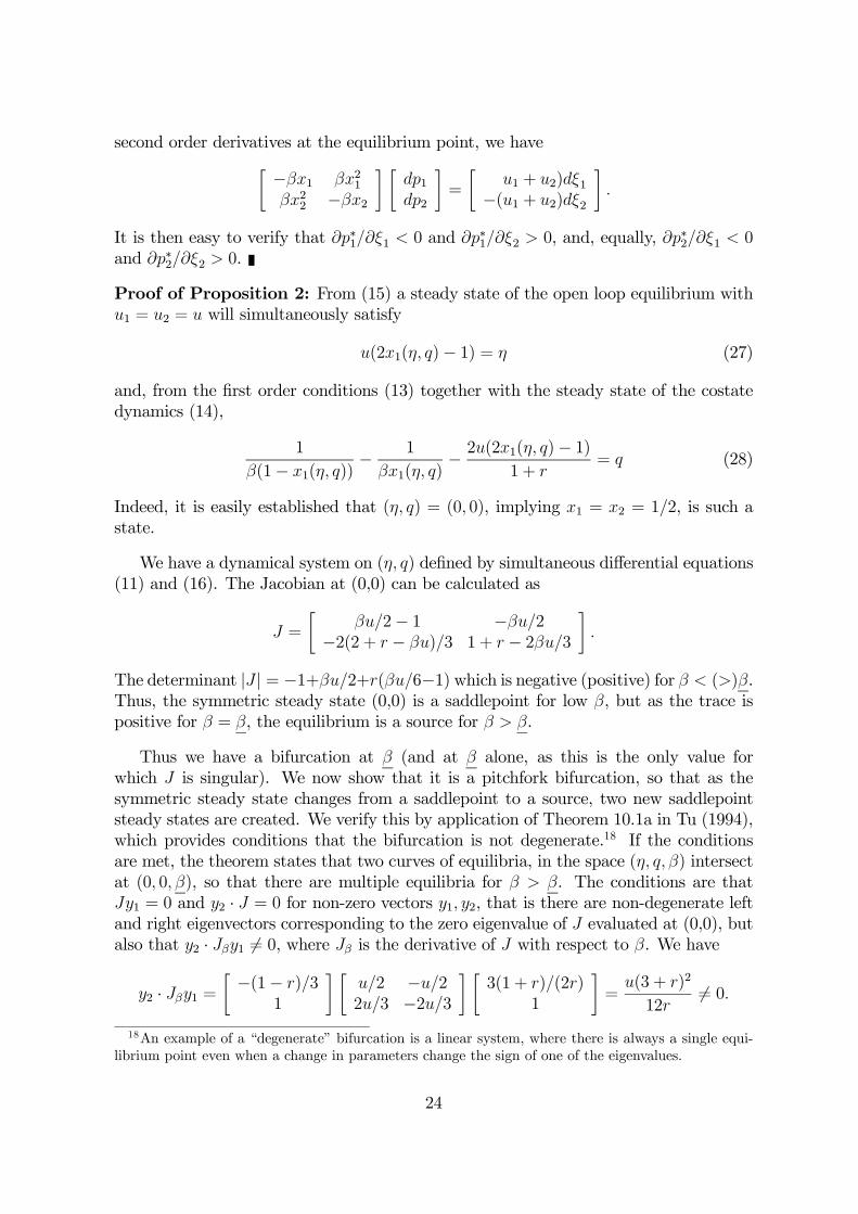
Proof of Proposition 2: From (15) a steady state of the open loop equilibrium withu1 = u2 = u will simultaneously satisfy

u(2x1(η, q)− 1) = η (27)

and, from the first order conditions (13) together with the steady state of the costatedynamics (14),

1

β(1− x1(η, q))− 1

βx1(η, q)− 2u(2x1(η, q)− 1)

1 + r= q (28)

Indeed, it is easily established that (η, q) = (0, 0), implying x1 = x2 = 1/2, is such astate.

We have a dynamical system on (η, q) defined by simultaneous differential equations(11) and (16). The Jacobian at (0,0) can be calculated as

J =

·βu/2− 1 −βu/2

−2(2 + r − βu)/3 1 + r − 2βu/3¸.

The determinant |J | = −1+βu/2+r(βu/6−1) which is negative (positive) for β < (>)β.Thus, the symmetric steady state (0,0) is a saddlepoint for low β, but as the trace ispositive for β = β, the equilibrium is a source for β > β.

Thus we have a bifurcation at β (and at β alone, as this is the only value forwhich J is singular). We now show that it is a pitchfork bifurcation, so that as thesymmetric steady state changes from a saddlepoint to a source, two new saddlepointsteady states are created. We verify this by application of Theorem 10.1a in Tu (1994),which provides conditions that the bifurcation is not degenerate.18 If the conditionsare met, the theorem states that two curves of equilibria, in the space (η, q, β) intersectat (0, 0, β), so that there are multiple equilibria for β > β. The conditions are thatJy1 = 0 and y2 · J = 0 for non-zero vectors y1, y2, that is there are non-degenerate leftand right eigenvectors corresponding to the zero eigenvalue of J evaluated at (0,0), butalso that y2 · Jβy1 6= 0, where Jβ is the derivative of J with respect to β. We have

y2 · Jβy1 =· −(1− r)/3

1

¸ ·u/2 −u/22u/3 −2u/3

¸ ·3(1 + r)/(2r)

1

¸=

u(3 + r)2

12r6= 0.

18An example of a “degenerate” bifurcation is a linear system, where there is always a single equi-librium point even when a change in parameters change the sign of one of the eigenvalues.

24

There must be two additional equilibria and they must be saddlepoints by verifi-cation that the bifurcation is of the supercritical pitchfork type.19 To do this, I applyresults from Kuznetsov (1995, Chapter 7). The dynamical system we consider is en-tirely symmetric, in that (η(η, q), q(η, q)) = −(η(−η,−q), q(−η,−q)). That is, if wewrite y = (η, q) and y = f(y, β), then Rf(y, β) = −f(Ry, β), where R = −I and I isthe identity matrix. Therefore, in the terminology of Kuznetsov, the dynamical systemis ZZ2-equivariant. Kuznetsov defines the set X− such that Ry = −y for y ∈ X−, thushere X− = IR2. Now, by Theorem 7.7 of Kuznetsov (1995), for a ZZ2-equivariant system,when the eigenvector corresponding to the zero eigenvalue is in the setX−, a bifurcationwill be of the pitchfork type. Now, as here X− is whole space, the eigenvector is inX−, and the bifurcation is a pitchfork. Furthermore, as we know from above that thenegative eigenvalue of J moves to positive as β increases, the bifurcation is supercritical.That is, we move from one to three equilibria, with the new equilibria having the samestability properties that the original equilibrium possessed for β < β. That is, they aresaddlepoints as claimed.

Proof of Proposition 3: The first step is to show that in any steady state whereη > 0, then q < η. The myopic duopoly equilibrium given by (9) defines implicitlya myopic level of relative price q(η). We have, clearly, q(0) = 0 and, by the implicitfunction theorem, ∂q(η)/∂η = ((1 − x1)

2 + x21)/((1 − x1)2 + x1) < 1. So, q(η) < η for

η > 0. Comparison of the myopic conditions (9) with the steady state of the dynamicequilibrium (15) shows that the dynamically optimal level q∗ will be less than q forη > q > 0 as this implies x1 < 1/2. So, q∗ < η in any steady state with η > 0. Fixq at its equilibrium level q∗(η) and substitute into the second equation in the steadystate conditions (15). Since, q∗(η) < η, we have by the properties of the logit choicefunction (5), limβ→∞ x1(η, q

∗(η)) = 1, and consequently limβ→∞ η∗(q∗(η)) = u1. Theresult follows.

Proof of Proposition 4: Inspection of the system of differential equations in (19)reveals that for x1 ∈ (0, 1), there is only one fixed point which is (θ1, θ2) = (u1, u2). Itis easy to prove (e.g. V = (θ1 − u1)

2 + (θ2 − u2)2 is a suitable Liapunov function) that

this fixed point is a global attractor, again for x1 ∈ (0, 1). But, given the functionalform (5), it is always true that x1 ∈ (0, 1).Proof of Proposition 5: If θ1(0) > u1 it is easy to demonstrate that θ1 convergesasymptotically to u1 but that θ1(t) > u1 for all finite t. One can then compare themyopic first order conditions (9) with (22) and see that p∗1 > p1 if µ1 > 0. Again,examining (23), it is clear that µ1 must always be positive to be able to attain its steadystate value which is positive. For p∗2, it is clear that ν2 must always be negative to beable to attain its steady state value which is negative. More formally, differentiating thefirst order conditions, and evaluating the second order derivatives at the equilibrium

19A pitchfork bifurcation occurs when, as the bifurcation parameter (here β) passes the criticallevel, there is a change from 1 to 3 equilibria. This is supercritical if, at the same time, the originalequilibrium changes from stable to unstable.

25

point, we have · −βx1 βx21βx22 −βx2

¸ ·dp1dp2

¸=

·(u1 − θ1)dµ1−(u1 − θ1)dν2

¸.

So, we have ∂p∗1/∂µ1 > 0 when θ1 > u1.

References

Arthur, W.B. (1993). On Designing Economic Agents that Behave like Human Agents.Journal of Evolutionary Economics 3, 1-22.

Bagwell, K., Riordan, M. (1991). High and declining prices signal product quality.American Economic Review 81, 224-239.

Benaïm, M. (1998). Recursive algorithms, urn processes and chaining number of chainrecurrent sets. Ergodic Theory and Dynamical Systems 18, 53-87.

Benaïm, M. (1999). Dynamics of Stochastic Algorithms. In: J. Azéma et al. (Eds),Séminaire de Probabilités XXXIII, Springer-Verlag: Berlin.

Bergemann, D., Välimäki, J. (1996). Learning and strategic pricing, Econometrica 64,1125-1149.

Bergemann, D., Välimäki, J. (2004). Monopoly pricing of experience goods, workingpaper.

Blume, A., Dejong, D.V., Neumann, G.R., Savin, N.E. (2002). Learning and commu-nication in sender-receive games: an econometric investigation, Journal of AppliedEconometrics 17, 225-247.

Börgers, T., Sarin, R. (2000). Naive reinforcement learning with endogenous aspira-tions, International Economic Review 41, 921-950.

Börgers, T., Sarin, R., Morales, A. (2004). Expedient and Monotone Learning Rules,Econometrica 72, 383-405.

Camerer, C., Ho, T-H. (1999). Experience-weighted attraction learning in normal formgames, Econometrica 67, 827-874.

Caplin, A., Nalebuff, B. (1991). Aggregation and imperfect competition: on the exis-tence of equilibrium, Econometrica 59, 25-59.

Cellini, R., Lambertini, L. (1998). A dynamic model of differentiated oligopoly withcapital accumulation, Journal of Economic Theory 83, 145-155.

Chintagunta, P.K., Rao, P.V. (1996). Pricing strategies in a dynamic duopoly: adifferential game model, Management Science 42, 1501-14.

26

Cooper, D., Garvin S., Kagel, J. (1997). Adaptive Learning versus Equilibrium Re-finements in an Entry Limit Pricing Game, Economic Journal 107, 553-575.

Ellison, G., Fudenberg, D. (1995). Word-of-Mouth Communication and Social Learn-ing, Quarterly Journal of Economics 110, 93-125.

ErdemT. et al. (1999). Brand equity, consumer learning and choice, Marketing Letters10, 301-318.

Erev, I., Barron, G. (2001). On adaptation, maximization and reinforcement learningamong cognitive strategies, working paper, Columbia University.

Erev, I., Haruvy, E. (2001). Variable pricing: a customer learning perspective, workingpaper.

Erev, I., Roth, A.E. (1998). Predicting how people play games: reinforcement learningin experimental games with unique, mixed strategy equilibria, American EconomicReview 88, 848-881.

Fudenberg, D., Levine, D. (1998). The Theory of Learning in Games. MIT Press:Cambridge, MA.

Gabaix, X., Laibson, D. (2003). Some industrial organization with boundedly rationalconsumers, working paper.

Harrington, J.E., Chang, M-H (2003). Co-Evolution of firms and consumers and theimplications for market dominance, Journal of Economic Dynamics and Control.

Ho, T-H., Chong J-K. (1999). A Parsimonious Model of SKU Choice: Familiarity-based Reinforcement and Response Sensitivity, working paper, Wharton School.

Ho, T-H., Chong J-K. (2003) A Parsimonious Model of Stock-Keeping Unit Choice,Journal of Marketing Research 40, 351-365

Hopkins, E. (2002). Two competing models of how people learn in games, Economet-rica 70, 2141-2166.

Hopkins, E., Posch, M. (2005). Attainability of Boundary Points under ReinforcementLearning, Games and Economic Behavior 53, 110-125.

Hopkins, E., Seymour, R. (2002). The stability of price dispersion under seller andconsumer learning, International Economic Review 43, 1157-1190.

Kamien, M.I., Schwartz, N.L. (2000). Dynamic Optimization. Second Edition. NorthHolland: Amsterdam.

Kirman, A.P. (1992). Whom or what does the representative individual represent,Journal of Economic Perspectives 6(2), 117-36.

27

Kirman, A.P., Vriend, N.J. (2001). Evolving market structure: an ACE model of pricedispersion and loyalty, Journal of Economic Dynamics and Control 25, 459-502.

Kuznetsov, Y.A. (1995). Elements of Applied Bifurcation Theory. Springer-Verlag:New York.

Milgrom, P., Roberts, J. (1986). Prices and advertising signals of product quality,Journal of Political Economy 94, 796-821.

Rabin, M., Schrag, J.L. (1999). First impressions matter: a model of confirmatorybias, Quarterly Journal of Economics 114, 37-82.

Rustichini, A. (1999). Optimal properties of stimulus-response learning models, Gamesand Economic Behavior 29, 244-73.

Sarin, R., Vahid, F. (1999). Payoff assessments without probabilities: a simple dy-namic model of choice, Games and Economic Behavior 28, 294-309.

Schmalensee, R. (1978). A model of advertising and product quality, Journal of Polit-ical Economy 86, 485-503.

Seetharaman, P.B., Chintagunta, P.K. (1998). A model of inertia and variety-seekingwith marketing variables, International Journal of Research in Marketing 15, 1-17.

Shapiro, C. (1983). Optimal pricing of experience goods, Bell Journal of Economics14, 497-507.

Smallwood D.E., Conlisk, J. (1979). Product quality in markets where consumers areimperfectly informed, Quarterly Journal of Economics 93, 1-23.

Sutton, J. (1991) Sunk Costs and Market Structure. MIT Press: Cambridge, MA.

Sutton, R.S., Barto, A.G. (1998) Reinforcement Learning: An Introduction. MITPress: Cambridge, MA.

Tu, P.N.V (1994). Dynamical Systems. Second Edition. Springer Verlag: Berlin.

Weisbuch G., Kirman A., Herreiner D. (2000). Market Organisation and TradingRelationships, The Economic Journal 110, 411-436.

28