AdaptingSingle-Loop

Control Systemsfor Nonlinear

Processes16.1 n INTRODUCTIONLinear control theory provides methods for the analysis and design of many successful control strategies. Control systems based on these linear methods are generally successful in the process industries because (l) the control system maintainsthe process in a small range of operating variables, (2) many processes are nothighly nonlinear, and (3) most control algorithms and designs are not sensitive toreasonable (±20%) model errors due to nonlinearities. These three conditions aresatisfied for many processes, but they are not satisfied by all; therefore, the controlof nonlinear processes must be addressed.

It is possible that the response of a nonlinear system could give better performance than a linear system and, therefore, a nonlinear control calculation mightbe better than any linear algorithm. However, there is no recognized, general nonlinear control theory that has been widely applied in the process industries. (Anexample of a nonlinear algorithm applied to level control is given in Chapter 18.)Therefore, the goal of the approaches in this chapter is to attain the performanceachieved with a well-tuned linear controller. To reach this goal, the control methodsin this chapter attempt to achieve a system that has a linear closed-loop relationship. If an element in the control loop is nonlinear, the approach applied here is tointroduce a compensating nonlinearity, so that the overall closed-loop system behaves approximately linearly. This compensating nonlinearity may be introducedin the control algorithm or in physical equipment, such as a sensor or final element.

The next section begins the analysis by introducing a method for determiningwhen nonlinearities significantly affect a control system. This analysis is extended

512

CHAPTER 16Adapting Single-LoopControl Systems forNonlinear Processes

to evaluate the proper fixed set of tuning constants for a linear PID controller appliedto a nonlinear process. If a fixed set of tuning constants and linear instrumentationare not satisfactory, improvements can be achieved by adapting either the controlcalculation or the equipment responses. First, a common method for adapting thecontroller tuning in real time to compensate for nonlinearities is presented. Thenthe same concept is applied to introduce compensating nonlinearities in selectedinstrumentation, such as the control valve, to improve performance.

16.2 01 ANALYZING A NONLINEAR PROCESS WITH LINEARFEEDBACK CONTROLA relatively simple process is analyzed in this section so that analytical modelscan be derived; the general approach is applicable to more complex processes.The process is shown in Figure 16.1a, which is the three-tank mixer consideredin Examples 7.2 and 9.2. The outlet concentration of the last tank is controlled byadjusting the addition of component A to the feed to the first reactor. The equationsdescribing the system are derived in Example 7.2 and summarized as follows:

^ b ( * a ) b + F A i x A ) A . , . . . . .* a o = „ , „ w i t h F A = K v v ( 1 6 . 1 )Pb + tA

*AO

db- XA\

% ~

L * A 2

"db"

(a)

*A3

Dis)- Gdis) hSPis) GJs) -(+>

CVis)

CVm(5)G M

Transfer FunctionsGcis) = ControllerGvis) = Transmission, transducer, and valveGpis) = ProcessGsis) = Sensor, transducer, and transmissionGdis) = Disturbance

FIGURE 16.1

VariablesCVis) = Controlled variableCVm(s) = Measured value of controlled variableDis) = DisturbanceEis) = ErrorSPCs) = Set point

ib)

Mixing process: (a) schematic; ib) control system block diagram.

vt dxAjdt

= iFA + FB)(xA(/_i) - xAi) for i = 1, 3 (16.2)

Note that the differential equations are nonlinear. We can linearize these equations,express the variables as deviations from the initial steady state, and take the Laplacetransforms to yield the transfer function model:

Gpis)Gds)Gds) Gpis)Gcis)•*A3

SPis) 1 + Gpis)Gds)Gds)Gds) 1 + GolCO °6'3)where the valve transfer function is a constant lumped into Gpis) and the sensorGsis) = 1.0.

Gods) = Gpis)Gds)Gds)Gds) « Gpis)Gcis)K,

(™ + l)3 Gds)(16.4)

513

Analyzing a NonlinearProcess with Linear

Feedback Control

where Kp = KvFbsJxaa —xAb)s

L (Fas + Fb,)2K„ = 0.0028

Vx =

(16.5)

(16.6)Fbs + FAs

This linearized model clearly demonstrates how the gain and time constantsdepend on the volumes, total flow, and compositions. We will consider the responseof the system for various values of one operating variable, the total flow rateiFA + Fb), which has the greatest variability for the situation considered here. Inthe scenario, the production rate changes periodically and remains nearly constantfor a long time (relative to the feedback dynamics) at each production rate. Theprocess dynamics are summarized in Table 16.1 for the range of flow variability(i.e., production rates) expected. The variation in the process dynamics due to thenonlinearity is not randomly distributed, because in this example the effect of anincrease in flow rate is to decrease the process gain and time constants concurrently.This type of correlation is typical for nonlinear processes and demonstrates theneed for careful analysis of the dynamic responses at different operating conditions.

TABLE 16.1

Summary of process dynamics and tuning for the three-tank mixing process*

Case Process parameters Control ler parameters

K, Kc T, Td

A 3 . 0 0 . 0 8 7 1 1 . 4 13.8 25.1 1.82B 4 . 0 0 . 0 6 4 8 . 6 18.6 19.0 1.4C 5 . 0 0 . 0 5 2 6 . 9 23.1 15.2 1.10D 6 . 0 0 . 0 4 3 5 . 7 27.9 12.7 0.92E 6 . 9 0 . 0 3 9 5 . 0 30.0 11.0 0.80

*For the combinations of process dynamicsmargin for each case is 1.7.

and tuning in this table, the gain

514

CHAPTER 16Adapting Single-LoopControl Systems forNonlinear Processes

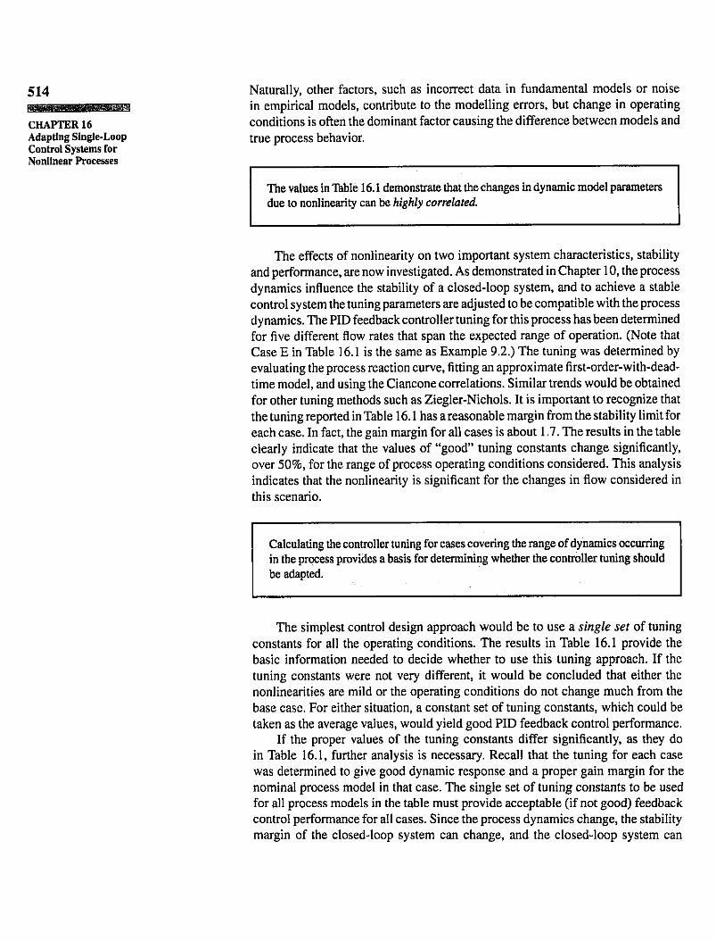
Naturally, other factors, such as incorrect data in fundamental models or noisein empirical models, contribute to the modelling errors, but change in operatingconditions is often the dominant factor causing the difference between models andtrue process behavior.

The values in Table 16.1 demonstrate that the changes in dynamic model parametersdue to nonlinearity can be highly correlated

The effects of nonlinearity on two important system characteristics, stabilityand performance, are now investigated. As demonstrated in Chapter 10, the processdynamics influence the stability of a closed-loop system, and to achieve a stablecontrol system the tuning parameters are adjusted to be compatible with the processdynamics. The PID feedback controller tuning for this process has been determinedfor five different flow rates that span the expected range of operation. (Note thatCase E in Table 16.1 is the same as Example 9.2.) The tuning was determined byevaluating the process reaction curve, fitting an approximate first-order-with-dead-time model, and using the Ciancone correlations. Similar trends would be obtainedfor other tuning methods such as Ziegler-Nichols. It is important to recognize thatthe tuning reported in Table 16.1 has a reasonable margin from the stability limit foreach case. In fact, the gain margin for all cases is about 1.7. The results in the tableclearly indicate that the values of "good" tuning constants change significantly,over 50%, for the range of process operating conditions considered. This analysisindicates that the nonlinearity is significant for the changes in flow considered inthis scenario.

Calculating the controller tuning for cases covering the range of dynamics occurringin the process provides a basis for determining whether the controller tuning shouldbe adapted.

The simplest control design approach would be to use a single set of tuningconstants for all the operating conditions. The results in Table 16.1 provide thebasic information needed to decide whether to use this tuning approach. If thetuning constants were not very different, it would be concluded that either thenonlinearities are mild or the operating conditions do not change much from thebase case. For either situation, a constant set of tuning constants, which could betaken as the average values, would yield good PID feedback control performance.

If the proper values of the tuning constants differ significantly, as they doin Table 16.1, further analysis is necessary. Recall that the tuning for each casewas determined to give good dynamic response and a proper gain margin for thenominal process model in that case. The single set of tuning constants to be usedfor all process models in the table must provide acceptable (if not good) feedbackcontrol performance for all cases. Since the process dynamics change, the stabilitymargin of the closed-loop system can change, and the closed-loop system can

become highly oscillatory or unstable for an improper choice of fixed tuning.Since instability and severe oscillations are to be avoided, the overriding concernis maintaining a reasonable stability margin for all expected process dynamics.

To ensure that the control system with varying process dynamics performsacceptably over the expected range of operation, the worst-case dynamics mustbe identified. This worst case gives the poorest control performance under thefeedback controller and is usually the closed-loop system closest to the stabilitylimit. The Bode plots of Gpis) for three of the cases in Table 16.1 are given inFigure 16.2. The results show that Case A has the lowest critical frequency andthe highest amplitude ratio at its critical frequency. This result conforms to ourexperience that processes with longer time constants are more difficult to control.Thus, Case A would be selected as the most difficult process operation, or theworst case, within the scenarios.

The Bode analysis of Gpis) is substantiated by the results in Table 16.1,which indicate that Case A has the least aggressive feedback controller, becausethe controller gain is smallest and integral time is largest. Applying the controllertuning from Case A would result in a stable system for all cases, albeit with poorperformance for some cases. Using a more aggressive set of tuning constants, CaseE, for example, would lead to good performance in some cases, but the closed-loopperformance would be very poor, and perhaps unstable, for other cases.

Dynamic simulations of closed-loop systems with various tunings are shownin Figures 16.3 and 16.4. The results in Figure 16.3a and b give the dynamicresponses of the closed-loop system, with controller tuning from Case A, for two

515

Analyzing a NonlinearProcess with Linear

Feedback Control

10"

o.6<

10i-5

10"

' | J _ i i i i i i i i i I I i ii—

C E ^

i i i i i i i i

^ 5

i i i i i i

io-'Frequency (rad/time)

10°

■5>-100

I "200

-300

-

1 I I I

-180°

i i i i i

A ^

1 1

E

l l l l l

i i i i i i i i i ' '10" io-'

Frequency (rad/time)10°

FIGURE 16.2

Bode plot for three-tank mixing system (cases defined in Table 16.1).

516

CHAPTER 16Adapting Single-LoopControl Systems forNonlinear Processes

K*

4.0

c3.0

50

0

£

4.0

3.0

50

0

0

FIGURE 16.3

250 250Timeia)

Timeib)

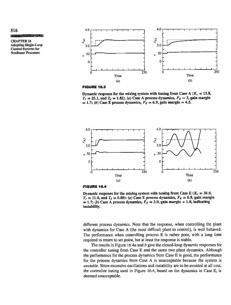
Dynamic respones for the mixing system with tuning from Case A iKc = 13.8,Ti = 25.1, and Td = 1.82). (a) Case A process dynamics, FB = 3, gain margin= 1.7; ib) Case E process dynamics, FB = 6.9, gain margin = 4.5.

4.0

3.0

> 50

0

M-.U — i — i — i i i — i — r — i — r

_ i / \ 7\ / ~

3.0 \ /^ ^ V \

> 50 /

0 -

i i i i I I I I I

0

FIGURE 16.4

250 250Timeia)

Timeib)

Dynamic respones for the mixing system with tuning from Case E (Kc = 30.0,T) = 11.0, and Td = 0.80): (a) Case E process dynamics, FB = 6.9, gain margin= 1.7; ib) Case A process dynamics, FB = 3.0, gain margin < 1.0, Indicatinginstability.

different process dynamics. Note that the response, when controlling the plantwith dynamics for Case A (the most difficult plant to control), is well behaved.The performance when controlling process E is rather poor, with a long timerequired to return to set point, but at least the response is stable.

The results in Figure 16.4a and b give the closed-loop dynamic responses forthe controller tuning from Case E and the same two plant dynamics. Althoughthe performance for the process dynamics from Case E is good, the performancefor the process dynamics from Case A is unacceptable because the system isunstable. Since excessive oscillations and instability are to be avoided at all cost,the controller tuning used in Figure 16.4, based on the dynamics in Case E, isdeemed unacceptable.

When the feedback controller tuning constants are fixed and the process dynamicschange, the fixed set of tuning constants selected should have the proper gain marginfor the most difficult process dynamics in the range considered. This approach willensure stability, but it may not provide satisfactory performance. For the example,the tuning from Case A is selected.

517

Improving NonlinearProcess Performance

through DeterministicControl LoopCalculations

This section has presented a manner for determining whether nonlinearitiessignificantly affect stability and control performance. The method is based onthe tuning and stability analysis of the system linearized about various operatingconditions. Also, a tuning selection criterion is given that is applicable when afixed set of tuning constants is used as the process dynamics vary. The goal ofthis criterion is to provide the best possible control performance, with constanttuning, while preventing instability or excessive oscillations. The resulting control performance may be unacceptably poor, providing sluggish compensation forsome cases; therefore, the next sections present common methods for improvingperformance, while preventing instability, by compensating for the nonlinearity.

16.3 Cl IMPROVING NONLINEAR PROCESS PERFORMANCETHROUGH DETERMINISTIC CONTROL LOOPCALCULATIONSThe approach described in the previous section can lead to poor control performance for two reasons. First, some process operating conditions lead to poor performance because of increased feedback dynamics (e.g., longer dead time and timeconstants). Second, the fixed values for the feedback controller tuning constantsare too "conservative" for some process operations. Clearly, one set of tuning values cannot prevent degradation in feedback control performance arising from thechanges in plant dynamics. However, modifying the tuning to be compatible withthe current process dynamics can maintain the feedback control performance closeto the best possible with the PID algorithm for whatever plant dynamics exist.

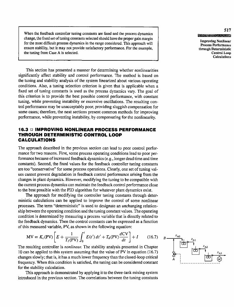
The approach for modifying the controller tuning constants through deterministic calculations can be applied to improve the control of some nonlinearprocesses. The term "deterministic" is used to designate an unchanging relationship between the operating condition and the tuning constant values. The operatingcondition is determined by measuring a process variable that is directly related tothe feedback dynamics. Then the control constants can be expressed as a functionof this measured variable, PV, as shown in the following equation:

MV = Kci?V) E +1

/ 'Jo Eit')dt' + Td(PV)dCV + / (16.7)T , i P V ) J n d t

The resulting controller is nonlinear. The stability analysis presented in Chapter10 can be applied to this system assuming that the value of PV in equation (16.7)changes slowly; that is, it has a much lower frequency than the closed-loop criticalfrequency. When this condition is satisfied, the tuning can be considered constantfor the stability calculation.

This approach is demonstrated by applying it to the three-tank mixing systemintroduced in the previous section. The correlations between the tuning constants

lA0

fer VA1

* ■

VA2

i*rt

518

CHAPTER 16Adapting Single-LoopControl Systems forNonlinear Processes

and the measured variable that indicates the change in process dynamics—in thisexample the flow—can be fitted by an equation or arranged in a lookup table.Equations for the example are given below for the range of operation in Table 16.1[3.1 < iFA + Fb) < 7.0] with the parameters determined by a least squares fit.

Kc = -5.64 + 7.368(FA + FB) - 0.3135(FA + FB)2Ti = 50.37 - 10.626(Fi4 + FB) +0.7164(Fi4 + FB):Td = 3.66 - 0.776(FA + FB) + 0.0525(FA + FB)2

(16.8)

The controller using tuning calculated by equations (16.8) can be applied tothe nonlinear mixing process. The resulting dynamic responses are essentially thesame as in Figure 16.3a and Figure 16.4a. The control performance is good forthe different flow rates because the tuning is modified to be compatible with theprocess dynamics. Note that the performance in Figure 16.4a is better than inFigure 16.3a, even though the controllers in both systems are well tuned, becausethe feedback dynamics in Case E are faster. Comparison with Figure 16.3b andFigure 16 Ab demonstrates the potential performance advantage of this approachover maintaining the tuning constants at fixed values. The procedure introducedin this example is summarized in Table 16.2.

The use of controller tuning modifications described in this section is oftenreferred to as gain scheduling, because early applications adjusted only the controller gain. With digital computers, all tuning constants can be easily adjustedwhen required to achieve the desired control performance.

If adequate control performance is achieved through adapting only the controller gain and the controller gain should be proportional to feed flow, gain scheduling can be implemented as part of modified feedforward/feedback control design.An example is given in Figure 16.5a for the feedforward and feedback control ofthe simple mixing system. The model for the system is

Xm —FAxA + FbXb

(16.9)FA + FB

The flows and compositions for this mixing process are assumed to be the same

TABLE 16.2

Criteria for the deterministic modification of controller tuning

Deterministic modification of tuning is appropriate when

1. Constant controller tuning values do not provide satisfactory control performancebecause of significant changes in operating conditions.

2. The nonlinearity can be predicted based on a process variable measured in real time.3. The relationship between the measurement and the process dynamics can be

determined either from a fundamental model or from empirically developed models.4. The changes in the process dynamics are at a frequency much lower than the

critical frequency of the control system.

31§

I

4

Feedforward

-C r̂-

I F e e d -(ac) back

ia)

~(§

©

Set point

[ f y V- H f c ]

■ $ $

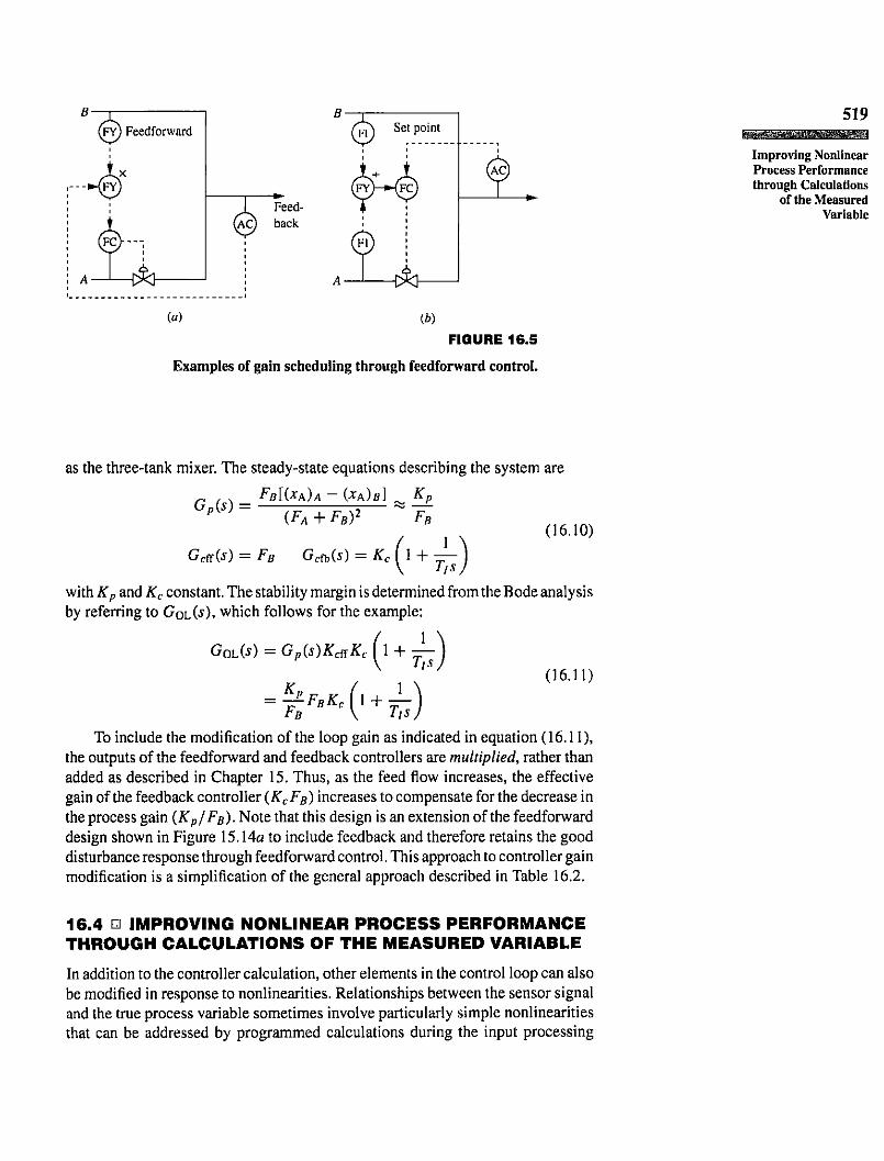
ib)FIGURE 16.5

Examples of gain scheduling through feedforward control.

519

Improving NonlinearProcess Performancethrough Calculations

of the MeasuredVariable

as the three-tank mixer. The steady-state equations describing the system are

Gpis) =FbKxa)a - ixA)B] . K

iFA + FB)2p

FB

Gcffis) = FB Gcfbis) = * < ( 1 + ^ )(16.10)

with Kp and Kc constant. The stability margin is determined from the Bode analysisby referring to GolC*), which follows for the example:

Gods) = Gpis)KcffKc (\ + ̂ M(16.11)

To include the modification of the loop gain as indicated in equation (16.11),the outputs of the feedforward and feedback controllers are multiplied, rather thanadded as described in Chapter 15. Thus, as the feed flow increases, the effectivegain of the feedback controller iKcFB) increases to compensate for the decrease inthe process gain {Kp/Fb). Note that this design is an extension of the feedforwarddesign shown in Figure 15.14a to include feedback and therefore retains the gooddisturbance response through feedforward control. This approach to controller gainmodification is a simplification of the general approach described in Table 16.2.

16.4 n IMPROVING NONLINEAR PROCESS PERFORMANCETHROUGH CALCULATIONS OF THE MEASURED VARIABLEIn addition to the controller calculation, other elements in the control loop can alsobe modified in response to nonlinearities. Relationships between the sensor signaland the true process variable sometimes involve particularly simple nonlinearitiesthat can be addressed by programmed calculations during the input processing

520

CHAPTER 16Adapting Single-LoopControl Systems forNonlinear Processes

phase of the control loop. Some examples are temperature (polynomial fit of thermocouple) and flow orifice (square root, density correction on AP). In additionto the linearization in the control loop, the availability of more accurate measuredvalues for use in control and process monitoring is another important benefit ofthese calculations.

16.5 a IMPROVING NONLINEAR PROCESS PERFORMANCETHROUGH FINAL ELEMENT SELECTION

Introducing a compensating nonlinearity in the control loop can be achieved byselecting appropriate control equipment to compensate for nonlinearities. The finalcontrol element, usually a valve, is the control loop element that is often modified inthe process industries, because the modifications involve little cost. Again, the explanation in this section assumes that the desired closed-loop relationship is linear;if another relationship is required, the approach can be altered in a straightforwardmanner.

Since the valve is normally very fast relative to other elements in the controlloop, only the gains of the elements are considered to vary. The linearized controlsystem is shown in the block diagram in Figure 16.1ft, and the loop gain for thissystem depends on the product of the individual gains.

Gods) = Gpis)Gds)Gds)Gsis)(16.12)= KpKvKcKsGpis)G*ds)G*ds)G*sis)

where the gains (£,) may be a function of operating conditions, and the dynamicelements of the transfer functions [G*is) with G*(0) = 1.0] do not change significantly with operating conditions. The manipulated variable in the majorityof control loops is a valve stem position iv), also referred to as the valve lift,which influences a flow rate. The feedback system behaves as though it is linearif Gods) does not change as plant operating conditions change. Thus, linearitycan be achieved, even if the process gain iKp) changes, as long as the changesdue to nonlinearities in the individual gains cancel. In this section, a method isdescribed in which the valve nonlinearity is designed to cancel an undesirableprocess nonlinearity, with the controller iKc) and sensor iKs) gains assumed tobe constant.

The final element selection is introduced through an example of flow control.The relationship between the controller output and the flow is often desired to belinear, so that the control system is linear. The relationship between the valve stemposition and the flow is given below (Foust et al., 1960; Hutchinson, 1976).

F = Fn C d v ) * P y100 V p (16.13)

w h e r e F = fl o wFmax = maximum flow through system with valve fully open

Cdv) = inherent valve characteristic, which is a function of vv = valve stem position (% open or closed)

APV = pressure difference across the valvep = fluid density

This is simply the expression for the flow through a restriction, with the variablev representing the valve stem position expressed in percent. The driving force forthe flow is the difference between the pressures immediately before and after thevalve, A Pv. The factor Cv is called the inherent valve characteristic and representsthe percentage of maximum flow at any given valve stem position at a constantpressure drop, usually the design value. The Cv is a function of the valve design,basically the size and shape of the opening and plug, which can be linear or any ofa selection of standard nonlinear relationships at the choice of the engineer. Threecommon inherent valve characteristics are shown in Figure 16.6.

In the typical process design, the pressures just before and after the valvechange as the flow rate changes, as shown in Figure 16.7 (Quance, 1979). Typically,the pressure at the pump outlet is not constant; it decreases as the flow through thepump increases (Labanoff and Ross, 1985; Karassik and McGuire, 1998). Also,the pressure drop from the valve to the pipe outlet increases as the flow increases.For the example process in Figure 16.7, the pressure drop from the valve outlet tothe end of the pipe could be calculated from the energy balance on the fluid, withlosses determined from friction factor correlations (Foust et al., 1960):

2

P2 = Fou, + APe + J2 A/W + APpipe + APfit (16.14)

521

Improving NonlinearProcess Performance

through Final ElementSelection

where Pou\ = outlet pressure (constant in this example)APe = pressure drop due to change in elevation

AFhx/(F) = pressure drop due to heat exchangers (/ = 1,2)AFpipe(F) = pressure drop in the pipe due to skin friction

APfit(F) = pressure drop in elbows and expansions due to form friction

100

4*2

c ,2

80 -70 -60 -

§ - 50403020100

-

/Quick-_ / opening

/ ' Linear

- / Equal-

I f 1 i i i ' '

percentage

i i i

1 0 2 0 3 0 4 0 5 0 6 0 7 0Valve stem, v (%)

80 90 100

FIGURE 16.6

Three standard control valve inherent characteristics.(Reprinted by permission. Copyright ©1976, Instrument Societyof America. From Hutchinson, J., ed., ISA Handbook of Control

Valves, 2nd ed.)

522

CHAPTER 16Adapting Single-LoopControl Systems forNonlinear Processes

td

2 T 1$3t~0~(SH

80

70 -

60 -

A 50 -

i n 40 -

30 -

20 -

10

\ ■— .—Cli

- APV i y

S ^ T lt̂ -"*"^

I I I I I " i 1 1 1 1

10 20 30 40 50 60 70 80 90 100 110 120F low (% o f des ign) f

Design valveFIGURE 16.7

Relationship between pressures and flow for a typical system.(Reprinted by permission. Copyright ©1979, Instrument Societyof America. From Quance, R., "Collecting Data for ControlValve Sizing," In. Tech., 55.)

Note that the last three pressure drop terms are functions of the flow rate (F). Dueto the functional relationships for Pi and P2, the pressure drop across the valve(AF„ = P\ - P2), decreases as the flow increases. This demonstrates that onlypart of the total pressure drop from the pump to the outlet is due to the valve; aconsiderable amount of the pressure drop is due to other frictional losses.

The goal of a linear system—a constant closed-loop relationship, GolCO—is achieved when the relationship between the controller output and controlledvariable is linear. In the case of flow control, the controller output can be takento be the valve position, and the controlled variable is the measured flow rate.Since the pressure drop across the valve shown in Figure 16.7 is not constant, therelationship between the controller output and the valve opening must introducea compensating nonlinearity for the overall gain to be constant. The nonlinearity can be introduced at low cost by selecting the appropriate valve characteristicCv. The typical nonlinearity applied for situations similar to Figure 16.7 is theequal-percentage characteristic curve shown in Figure 16.6. The use of an equal-percentage valve in a process similar to that shown in Figure 16.7, in which thepressure drop decreases with flow, usually results in an approximately linear relationship between the valve stem position and flow. An experimental investigationof the application of an equal-percentage valve for the process described in Figure16.7 resulted in the desired linear relationship shown in Figure 16.8. Note that the

523

4 0 6 0Valve stem, v (%)

100

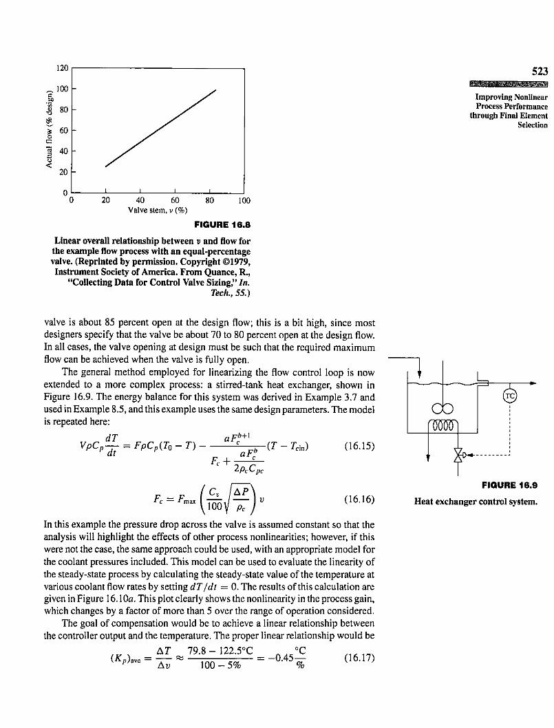
FIGURE 16.8

Linear overall relationship between v and flow forthe example flow process with an equal-percentagevalve. (Reprinted by permission. Copyright ©1979,Instrument Society of America. From Quance, R.,

"Collecting Data for Control Valve Sizing," In.Tech., 55.)

Improving NonlinearProcess Performance

through Final ElementSelection

valve is about 85 percent open at the design flow; this is a bit high, since mostdesigners specify that the valve be about 70 to 80 percent open at the design flow.In all cases, the valve opening at design must be such that the required maximumflow can be achieved when the valve is fully open.

The general method employed for linearizing the flow control loop is nowextended to a more complex process: a stirred-tank heat exchanger, shown inFigure 16.9. The energy balance for this system was derived in Example 3.7 andused in Example 8.5, and this example uses the same design parameters. The modelis repeated here:

VpCp^ = FpCpiTo-T)-aFcb+l

F, +aFl iT - Tcm)

^•Pc^pc

Fr = F„ C^ AP_100V Oe

(16.15)

(16.16)

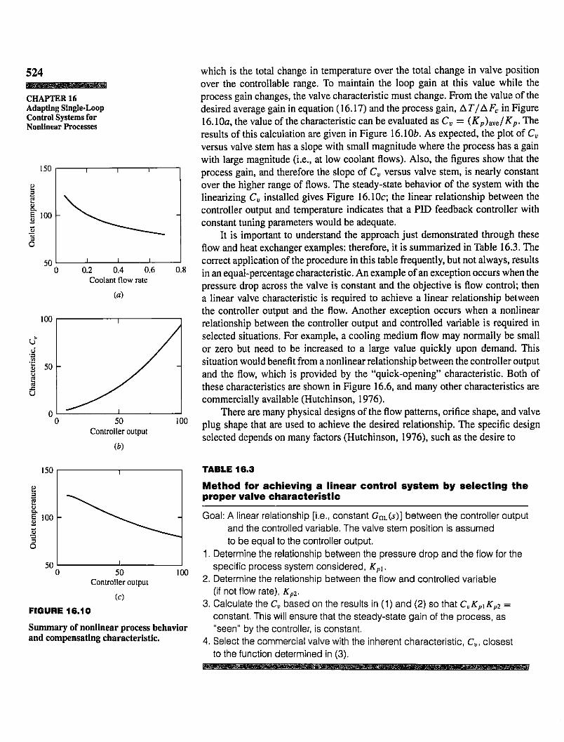
In this example the pressure drop across the valve is assumed constant so that theanalysis will highlight the effects of other process nonlinearities; however, if thiswere not the case, the same approach could be used, with an appropriate model forthe coolant pressures included. This model can be used to evaluate the linearity ofthe steady-state process by calculating the steady-state value of the temperature atvarious coolant flow rates by setting dT/dt = 0. The results of this calculation aregiven in Figure 16.10a. This plot clearly shows the nonlinearity in the process gain,which changes by a factor of more than 5 over the range of operation considered.

The goal of compensation would be to achieve a linear relationship betweenthe controller output and the temperature. The proper linear relationship would be

, „ v A T 7 9 . 8 - 1 2 2 . 5 ° C „ ° C(*')ave = A^% 100-5% = ~0A5% (16.17)

u

mm(rc)

x d -

FIGURE 16.9

Heat exchanger control system.

524

CHAPTER 16Adapting Single-LoopControl Systems forNonlinear Processes

u

0 . 2 0 . 4 0 . 6Coolant flow rate

ia)

50Controller output

ib)

which is the total change in temperature over the total change in valve positionover the controllable range. To maintain the loop gain at this value while theprocess gain changes, the valve characteristic must change. From the value of thedesired average gain in equation (16.17) and the process gain, AT/AFC in Figure16.10a, the value of the characteristic can be evaluated as Cv = iKp)x,c/Kp. Theresults of this calculation are given in Figure 16.10ft. As expected, the plot of Cvversus valve stem has a slope with small magnitude where the process has a gainwith large magnitude (i.e., at low coolant flows). Also, the figures show that theprocess gain, and therefore the slope of Cv versus valve stem, is nearly constantover the higher range of flows. The steady-state behavior of the system with thelinearizing Cv installed gives Figure 16.10c; the linear relationship between thecontroller output and temperature indicates that a PID feedback controller withconstant tuning parameters would be adequate.

It is important to understand the approach just demonstrated through theseflow and heat exchanger examples: therefore, it is summarized in Table 16.3. Thecorrect application of the procedure in this table frequently, but not always, resultsin an equal-percentage characteristic. An example of an exception occurs when thepressure drop across the valve is constant and the objective is flow control; thena linear valve characteristic is required to achieve a linear relationship betweenthe controller output and the flow. Another exception occurs when a nonlinearrelationship between the controller output and controlled variable is required inselected situations. For example, a cooling medium flow may normally be smallor zero but need to be increased to a large value quickly upon demand. Thissituation would benefit from a nonlinear relationship between the controller outputand the flow, which is provided by the "quick-opening" characteristic. Both ofthese characteristics are shown in Figure 16.6, and many other characteristics arecommercially available (Hutchinson, 1976).

There are many physical designs of the flow patterns, orifice shape, and valveplug shape that are used to achieve the desired relationship. The specific designselected depends on many factors (Hutchinson, 1976), such as the desire to

0 50Controller output

ic)FIGURE 16.10

100

Summary of nonlinear process behaviorand compensating characteristic.

TABLE 16.3Method for achieving a linear control system by selecting theproper valve characteristicGoal: A linear relationship [i.e., constant G0l(*)] between the controller output

and the controlled variable. The valve stem position is assumedto be equal to the controller output.

1. Determine the relationship between the pressure drop and the flow for thespecific process system considered, Kpl.

2. Determine the relationship between the flow and controlled variable(if not flow rate), Kp2.

3. Calculate the Cv based on the results in (1) and (2) so that CvKpXKp2 =constant. This will ensure that the steady-state gain of the process, as"seen" by the controller, is constant.

4. Select the commercial valve with the inherent characteristic, C„, closestto the function determined in (3).

1. Have tight closing (i.e., no flow) when the controller output is 0% (or 100%for a fail-open valve)

2. Prevent sticking or clogging when the fluid is viscous or is a slurry3. Accurately control the flow over a specified range4. Reduce the pressure loss due to the valve, to conserve energy

The reader is cautioned that the selection of the proper control valve requiresmore information than is provided in this brief introduction. Details of typicalvalves, along with pictures of the internal details, are available and should beconsulted (Hutchinson, 1976; Andrew and Williams, 1979,1980; Driskell, 1983).Also, engineering standards for sizing calculations and selection are available formany common situations (ISA, 1992).

Finally, it should be noted that a nonlinearity can be added to the controllercalculation in place of the nonlinear valve characteristic. Many commercial digitalcontrollers have the facility to introduce a nonlinearity after the control algorithm,in the output processing phase, via a general polynomial. However, the use of thevalve characteristic is still the most common means in practice for compensatingfor simple process gain nonlinearities.

525l

Improving NonlinearProcess Performance

through CascadeDesign

16.6 Q IMPROVING NONLINEAR PROCESS PERFORMANCETHROUGH CASCADE DESIGNOther particularly simple nonlinearities can be addressed through cascade designthat compensates for nonlinearities in the secondary, resulting in a (nearly) linearprimary control system. One example encountered often in the process industriesis maintaining two quantities in a desired proportion. An example of blending isshown in Figure \6.5b, although the concept applies to other proportions, suchas reboiler to feed in a distillation tower or reactant ratio in a chemical reactor.The feedback controller can adjust the set point of the ratio controller as shown inFigure 16.5ft. This is really another example of feedforward and feedback beingcombined as a product rather than a sum; thus, Figure 16.5a and b are alternativesolutions to the same control design problem.

A cascade can also provide compensation for nonlinearities in other control designs. An example is shown in Figure 16.11, in which the relationship

&& - * ■

r®-&

H & - *

i a ) i b )FIGURE 16.11

Example of cascade control applied to linearize the loop.

526

CHAPTER 16Adapting Single-LoopControl Systems forNonlinear Processes

between the level and the level controller output is desired to be linear. Followingthe arguments in this section, the valve in Figure 16.11a would normally havean equal-percentage characteristic so that the relationship between the controlleroutput and flow would be approximately linear. However, since the flow controllerin Figure 16.11ft is a fast loop, the relationship between the primary controlleroutput and the flow would be linear, regardless of how well the characteristic compensated for other nonlinearities. Thus, the level control system is linearized as aresult of the cascade design. Notice that the cascade strategy retains the advantagesof improved disturbance response explained in Chapter 14.

16.7 □ REAL-TIME IMPLEMENTATION ISSUES

Adaptive methods involving real-time calculations are relatively straightforward toimplement; however, a few special considerations should be included. Some of themethods for adapting tuning are based on one or more measurements, and should ameasurement not represent the true process conditions because of a sensor failure,the resulting tuning constants could be far from the proper values, leading to pooror even unstable performance. Thus, the measurement(s) used in the updating calculations should be checked for validity before being used to calculate the tuning.An example is checking the consistency of a flow measurement with associatedflow rates in the process to ensure that a realistic flow is being used to updatetuning. In addition, the value of the measured variable used in the correlations, asin equations (16.8), should be limited to the range over which the correlation isvalid. This practice serves two purposes:

1. Error due to an unrecognized sensor failure is limited.2. Extrapolation of a correlation beyond its region of applicability is prevented.

An issue that may not have been apparent in the previous sections is the ever-present need for defining the desired control performance. The tuning correlationsmust reflect the performance desired; thus, the tuning correlations selected must bebased on control objectives consistent with the performance desired in the plant.As will be explained in Parts V and VI, tight control of one variable may degradethe control performance of another, more important variable because of processinteraction. Thus, the performance goals of all control loops must be determinedconsidering the overall process performance, which may lead to loose tuning forselected loops.

Also, it would be wise to provide the facility to fine-tune the controller tuningconstants while retaining the correlations. One simple method would be to provide an adjustable parameter in equations (16.8). The engineer could adjust theparameter to achieve improved performance at one operating condition, and theparameter would be unchanged for other operating conditions.

16.8 m ADDITIONAL TOPICS IN CONTROL LOOPADAPTATIONAll of the methods described in detail in this chapter are based on the assumptionthat the change in process dynamics can be predicted. This assumption, whichleads to the compensating calculations and equipment designs, is not always valid.

For example, the effect of acid flow on pH (i.e., the shape of a pH curve) canchange substantially due to changes in the buffering agents present; the effectof temperature on reactor conversion can depend on the activity of the catalyst.Therefore, there are situations in which deterministic methods are not appropriate.One response to this situation would be to detune the controller substantially andaccept the performance degradation. Better performance would be possible withan adaptive method that could "learn" the process dynamics from the real-timesystem behavior and retune the controller based on the updated knowledge ofprocess dynamics. Two general retuning approaches are used in this situation:

527

Additional Topics inControl Loop

Adaptation

1. Periodic adaptive tuning at the request of a person, which is applicable whenthe dynamics change infrequently

2. Continuous adaptive retuning, which is applicable when the dynamics changefrequently

The analysis of these approaches requires more advanced mathematics than isconsistent with the level of this book; however, a few of the methods are introducedin the following paragraphs.

Periodic Retuning Based on Model IdentificationIn this approach an empirical model identification method is implemented to determine the dynamic model of the process, Gpis)Gds)Gsis). The model fittingcould use one of the methods described in Chapter 6 or other statistically basedmethods. Based on this model, the method can automatically introduce updatedtuning using an appropriate controller tuning method. Note that this method introduces perturbations in the manipulated variable, which will disturb the process,but only when a person requests a retuning.

Periodic Retuning Based on Empirical Identification of theCritical ConditionsThe Bode stability criterion highlighted the importance of the feedback system atthe critical frequency. The feedback system's stability and controller tuning can bebased on the amplitude ratio at the critical frequency, | God<*>c) I• Thus, some methods of adaptive tuning determine the critical conditions empirically. One possibleapproach would be to automate the Ziegler-Nichols continuous cycling experiment described in Section 10.8, Interpretation IV; however, this approach wouldintroduce large, prolonged disturbances. A more successful approach uses thisprinciple with a relay in place of the controller to determine the same information,with smaller disturbances to the plant (Astrom and Hagglund, 1984).

Continuous Retuning Based on StatisticsIt is possible to identify the process dynamics and determine how to modify thetuning without introducing external perturbations, as long as some disturbancesoccur in the process. Approaches to formulating and solving this problem are givenin Astrom and Wittenmark (1989).

528

CHAPTER 16Adapting Single-LoopControl Systems forNonlinear Processes

Continuous Retuning Based on RulesFine tuning of closed-loop systems based on the response to set point changes wasdiscussed in Chapter 9. This concept can be applied to disturbance responses sothat external perturbations are not necessary; then the method can be automated toachieve continuous retuning. In one commercial system the control performance isdefined by the engineer in terms of (1) controlled-variable damping and overshoot,(2) expected noise levels, and (3) bounds on the controller tuning constants (Bristol,1977; Kraus and Myron, 1984). The retuning method uses rules to adjust the tuningconstants to achieve the desired performance.

16.9 m CONCLUSIONSModification of an element in the closed-loop system may be needed to attain high-performance feedback control when the feedback dynamics change. The threemajor steps are given in Table 16.2 for evaluating deterministic approaches forcompensating for nonlinearities. The first step is to determine whether the processdynamics change significantly over the range of operation. If a fundamental analytical model is available, the linearized expression can be evaluated through therange of operating variables to determine whether the gain, dead time, and timeconstants change significantly. If no analytical model is available, several linearmodels can be determined through empirical identification at various operatingconditions. The variability in the tuning and degradation in performance due tothe nonlinearities can be determined as explained in Section 16.2. Since controlobjectives are different from plant to plant, it is not possible to give a generallyapplicable threshhold for when the nonlinearity is "significant." However, sincemodelling errors of ±20% are expected in identification, nonlinearities causingmodel parameter variations of this magnitude or less would normally not be considered significant.

The approaches presented in this chapter are summarized in Table 16.4. Theorder of presentation is from simplest and most reliable to most complex andchallenging to implement. Generally, the engineer will apply the methods in theorder presented in the table, proceeding only to the method needed to achieveacceptable performance.

If the variability is significant and it can be predicted based on real-timemeasurements, an element can be introduced to linearize the control loop by compensating for the nonlinearity. The compensating element can be in any of thethree categories of the control calculation: input processing, control algorithm, oroutput processing. It can also be included in the control equipment, specifically inthe final control element.

If the variability in dynamics is significant but cannot be predicted usingcorrelations, one approach is to detune the feedback controller so that it is stablefor all dynamics encountered. Naturally, this approach will result in a degradationin performance. Another approach is to modify the tuning of the controller basedon some information of the real-time dynamic behavior of the system. Variousmethods are available, and references are provided.

Finally, the limits of the adapting approach should be recognized. First, a greatstrength of feedback control is that it does not require a highly accurate model.Thus, reasonable model errors can be tolerated with little degradation in controlperformance. Second, the adaptations require some time for the method to recog-

nize the change in process behavior and introduce the compensation to the tuning(or other element of the loop). Thus, if the process dynamics are changing witha frequency near the critical frequency of the feedback control loop, an adaptiveapproach will not be able to introduce the compensation quickly enough. This

529

Conclusions

TABLE 16.4

Summary of methods to compensate control systems for nonlinearities

Compensation for Additional effects onDescription nonlinearity Example control performance

Measurement Calculation to compensate Square root of orifice Improved accuracy forfor nonlinear flow meter process monitoringsensor (Figure 12.5)

Final element Final element selected Valve characteristic toto compensate for account for changes inprocess nonlinearity pressure (Figures 16.6

and 16.7)Cascade control Select secondary set Level-flow cascade Improved response to

point that has linear (Figure 16.11) secondary disturbancesrelationship with primary

Detune Determine single set Three-tank mixing Poor performanceof tuning constants process (Table 16.1, can resultfor the range of operating Case A tuning)conditions

Gain schedule Calculate the controllergain based on real-timemeasurementMultiply feedforward Figure 16.5 Feedforwardand feedback (where compensation forthis leads to proper measured disturbancegain scheduling)

Controller Calculate tuning based Three-tank mixingtuning on a process model process [equation

and real-time (16.8)]measurement

Occasionally Empirically determine Relay method of Undesired variationretune key model finding critical during (infrequent)

characteristics and conditions (Astrom and retuningtune controller according Hagglund, 1984)to preselectedperformance criteria

Continuously Empirically determine On-line identificationretune key model

characteristics and tunecontroller according topreselected performancecriteria

530

CHAPTER 16Adapting Single-LoopControl Systems forNonlinear Processes

limitation also holds when an infrequent change in process dynamics is large andabrupt: adaptation may not be able to detect the situation rapidly enough. Finally,the reader is advised to establish the potential improvement using the first entriesin Table 16.4 before attempting the substantially more complex approaches in latertable entries.

REFERENCESAndrews, W., and H. Williams, Applied Instrumentation in the Process Indus

tries (2nd ed.), 2 vols., Gulf Publishing, Houston, TX, 1979,1980.Astrom, K., and T. Hagglund, "Automatic TAining of Simple Regulators with

Specifications on Phase and Amplitude Margins," Automatica, 20, 645-651 (1984).

Astrom, K., andB. V/ittenmark, Adaptive Control, Addison-Wesley, Reading,MA, 1989.

Bristol, E., "Pattern Recognition: An Alternative to Parameter Identificationin Adaptive Control" Automatica, 13, 197-202(1977).

Chalfin, S., "Specifying Control Valves," Chem. Eng., 81, 105-114 (October1974).

Driskell, L., Control Valve Selection and Sizing, Instrument Society of America, Research Triangle Park, NC, 1983.

Foust, A., in Chapter 3, Principles of Unit Operations, Wiley, New York, 1960.Hutchinson, J. (ed.), ISA Handbook of Control Valves (2nd ed.), Instrument

Society of America, Research Triangle Park, NC, 1976.ISA, ISA Standards and Practices (11th ed.), Instrument Society of America,

Research Triangle Park, NC, 1992.Karassik, I., and T. McGuire, Centrifugal Pumps, 2nd ed., Chapman and Hall,

New York, 1998.Kraus, T., and T. Myron, "Self-Tuning PID Controller Uses Pattern Recogni

tion Approach," Cont. Eng., 31, 106-111 (June 1984).Labanoff, V, and R. Ross, Centrifugal Pumps, Design and Applications, Gulf

Publishing, Houston, TX, 1985.Quance, R., "Collecting Data for Control Valve Sizing," In. Tech., 55 (Novem

ber 1979).

ADDITIONAL RESOURCES

Computer programs and exercises for several adaptive tuning methods have beenprepared by

Roffel, B., P. Vermeer, and P. Chin, Simulation and Implementation of Self-Tuning Controllers, Prentice-Hall, Englewood Cliffs, NJ, 1989.

Adaptive tuning of PID and other feedback control algorithms are presentedat an advanced level in

Astrom, K., and T. Hagglund, Automatic Tuning of PID Controllers, ISA,Research Triangle Park, NC, 1988.

Questions

Goodwin, G., and K. Sin, Adaptive Filtering, Prediction, and Control, Prentice- 531Hall, Englewood Cliffs, NJ, 1984.

A particularly challenging situation occurs when the process gain changessign as operating conditions change. An industrial process where this occurs isdiscussed in

Dumont, G., and Astrom, K., "Wood Chip Refiner Control," IEEE Cont. Sys.,8, 38-43 (1988).

Some industrial examples of adaptive control are given in the following references.

Piovoso, M., and J. Williams, Self-Tuning Control ofpH, ISA Paper no. 0-87664-826-x, 1984.

Vermeer, P., B. Roffel, and P. Chin, "An Industrial Application of an AdaptiveAlgorithm for Overhead Composition Control," Proc. Auto. Cont. Conf,St. Paul, MN, 1987.

Whately, M., and D. Pott, "Adaptive Gain Improves Reactor Control," Hydro.Proc, 75-78 (May 1988).

QUESTIONS16.1. Consider the three-tank mixing example process, but with the outlet con

centration of component A changed to 50 percent in all cases. Recalculatethe values in Table 16.1 for the same changes in the flow rate of stream B.Compare and comment on the similarities and differences.

16.2. Answer each of the following questions, with a full explanation of youranswer.id) Could closed-loop frequency response, as explained in Section 13.3, be

used to determine when feedback controller tuning should be adaptedfor changes in operating conditions?

ib) Review all cascade examples in Section 14.7 and determine whethereach results in a (nearly) linear relationship between the secondary andprimary. Would the single-loop control (primary to valve) be significantly nonlinear?

ic) Review all of the feedforward-feedback control designs in Section 15.7and for each, recommend how to combine the feedforward and feedback signals (add, multiple, divide, other) to provide the best tuningcompensation for the measured disturbances.

id) The discussion and examples in this chapter involved feedback control. Discuss whether there is any advantage to adapting the adjustableparameters in a feedforward controller. If yes, discuss how this couldbe evaluated and the proper values determined.

16.3. Recalculate the tuning in Table 16.1 using the Ziegler-Nichols closed-looptuning method. Compare the similarities and differences of the effect ofFb on the tuning for the two tuning methods. Which tuning would yourecommend using?

532 16.4. Based on the information in question 9.10, would you recommend auto-wmMkMdmmmmim matic deterministic retuning of the feedback control system? If yes, deter-CHAPTER16 mine the measured variable and the tuning constants as a function of theA d a p t i n g S i n g l e - L o o p m e a s u r e d v a r i a b l e .Control Systems forNonlinear Processes 16.5. Based on the information in question 10.2, would you recommend auto

matic deterministic retuning of the feedback control system? If yes, determine the measured variable and the tuning constants as a function of themeasured variable.

16.6. You have been given the task of developing a rule-based adaptive tuningmethod for use with a PID controller. Also, the introduction of any perturbations by the method has been prohibited. Develop a set of rules thatcan be applied to normal operating data (with disturbances) to improve theperformance gradually by adjusting the controller tuning constants. Remember to consider both the controlled and manipulated variables whenevaluating performance.

16.7. In some control designs, the location of the sensor can be changed; onemethod for changing the effective sensor location is switching betweensample tap locations that feed an analyzer. In this question we considerthe dynamic system described in Example 5.2, Case 1. The original feedback PI controller measured Y4 and adjusted the input to the system; themodified feedback PI controller measures Y3 and adjusts the input to thesystem. Calculate the tuning for both PI controllers and decide whether thecontroller tuning should be adjusted when the sensor is switched.

16.8. The stirred-tank heat exchanger in Section 16.5 experiences changes in thefeed inlet temperature of 120 to 170°C and in the coolant inlet temperatureof 20 to 30°C. These temperature changes occur independently, and the feedflow and temperature set point remain constant at their base-case values.Discuss the need for adapting the feedback PI controller tuning constantsand, if necessary, provide correlations for the valve characteristic and tuningas appropriate.

16.9. Design feedforward-feedback control for the chemical reactor in Example15.1 for input disturbances in both feed composition, A2, and feed flow,Fl. Pay particular attention to how the feedforward and feedback signalsshould be combined. Is there a need for adapting the feedback tuning fordisturbances? Can this be achieved in combination with the feedforwardcontrol? Is there a need to adapt the feedforward controller parameters?Since you do not have fundamental models for this system, answer thisquestion based on your qualitative understanding of the behavior of theprocess equipment.

16.10. The behavior of the heat exchanger in the recycle system in Example 5.3varies due to fouling. Experience has shown that Gh2 changes within therange of 0.20 to 0.32 about its nominal value of 0.30. Determine whetherthis change is significant. If so, how could deterministic controller adaptation be implemented?

16.11. Sometimes process equipment has to be removed from service occasionallyfor maintenance. Consider a multiple-tank mixing process that is basically

the mixing tank process in Example 7.2, but modified to have between two 533and four tanks, depending on the equipment availability. Determine how w»««!^*iH^«M»sithe feedback controller tuning has to be modified for the situations of two, Questionsthree, and four tanks in the feedback process. Also, compare the controlperformance for these three situations.

16.12. Level control is to be added to the draining tank process in Example 3.6.The controller adjusts the opening of a valve in the exit pipe at the baseof the tank, and essentially all of the pressure drop in the pipe and valveoccurs across the valve. Determine the valve characteristic that will yielda linear relationship between the controller output and the level. The inletflow varies from 50 to 150 m3/h.

16.13. In some feedback control systems the manipulated variable can be changed,usually by selecting the position of a switch at the controller output thatdirects the signal to one of the possible manipulated variables. For the following cases, determine whether the difference in feedback dynamics issignificant enough to require changing the tuning depending on the manipulated variable selected for the controller output.ia) For a distillation column, the controlled variable is the light key in the

distillate, XD, and the two manipulated variables are the reflux flow,FMr, and the vapor boilup, VMq. For dynamic models, refer to Figure5.17.

ib) For a single, isothermal CSTR, the controlled variable is the effluentreactant concentration, CA, and the two manipulated variables are theinlet concentration, Cao, and the total feed flow rate, F. For dynamicmodels, refer to Example 5.5.

ic) For an open-top liquid tank, the controlled variable is the liquid level,and the two manipulated variables are the valves in the two outlet pipes.The process is sketched in Figure Q1.9a.

16.14. Question 13.1 describes a process with feedback control and changes inoperating conditions, id) through if). For each change in operating conditions, determine whether it is necessary to adapt the feedback controllertuning, and if so, how the adaptation could be implemented automatically.

16.15. Consider a series of three isothermal CSTRs, each with the physical designparameters of the process in Example 3.5. The base case operating conditions are the same as the example: F = 0.085, Cao = 0.925, and k = 0.50.The composition of reactant A in the third reactor is controlled by adjusting the feed composition, CAo- Determine id) the steady-state operatingconditions for this base case, ib) the linearized model for the system, and(c) PID feedback tuning for this base case system. Then determine whetherthe controller tuning must be adjusted if the feed flow rate changes from0.085 to 0.20.