ControlObjectives and

Benefits2 . 1 □ I N T R O D U C T I O N

The first chapter provided an overview of process control in which the close association between process control and plant operation was noted. As a consequence,control objectives are closely tied to process goals, and control benefits are closelytied to attaining these goals. In this chapter the control objectives and benefitsare discussed thoroughly, and several process examples are presented. The controlobjectives provide the basis for all technology and design methods presented insubsequent chapters of the book.

While this book emphasizes the contribution made by automatic control, control is only one of many factors that must be considered in improving processperformance. Three of the most important factors are shown in Figure 2.1, whichindicates that proper equipment design, operating conditions, and process controlshould all be achieved simultaneously to attain safe and profitable plant operation.Clearly, equipment should be designed to provide good dynamic responses in addition to high steady-state profit and efficiency, as covered in process design coursesand books. Also, the plant operating conditions, as well as achieving steady-stateplant objectives, should provide flexibility for dynamic operation. Thus, achieving excellence in plant operation requires consideration of all factors. This bookaddresses all three factors; it gives guidance on how to design processes and selectoperating conditions favoring good dynamic performance, and it presents automation methods to adjust the manipulated variables.

Safe,ProfitablePlantOperation

FIGURE 2.1Schematic representation of three

critical elements for achieving excellentplant performance.

20

CHAPTER 2Control Objectivesand Benefits

Control Objectives

1. Safety2. Environmental Protection3. Equipment Protection4. Smooth Operation

and Production Rate5. Product Quality6. Profit7. Monitoring and Diagnosis

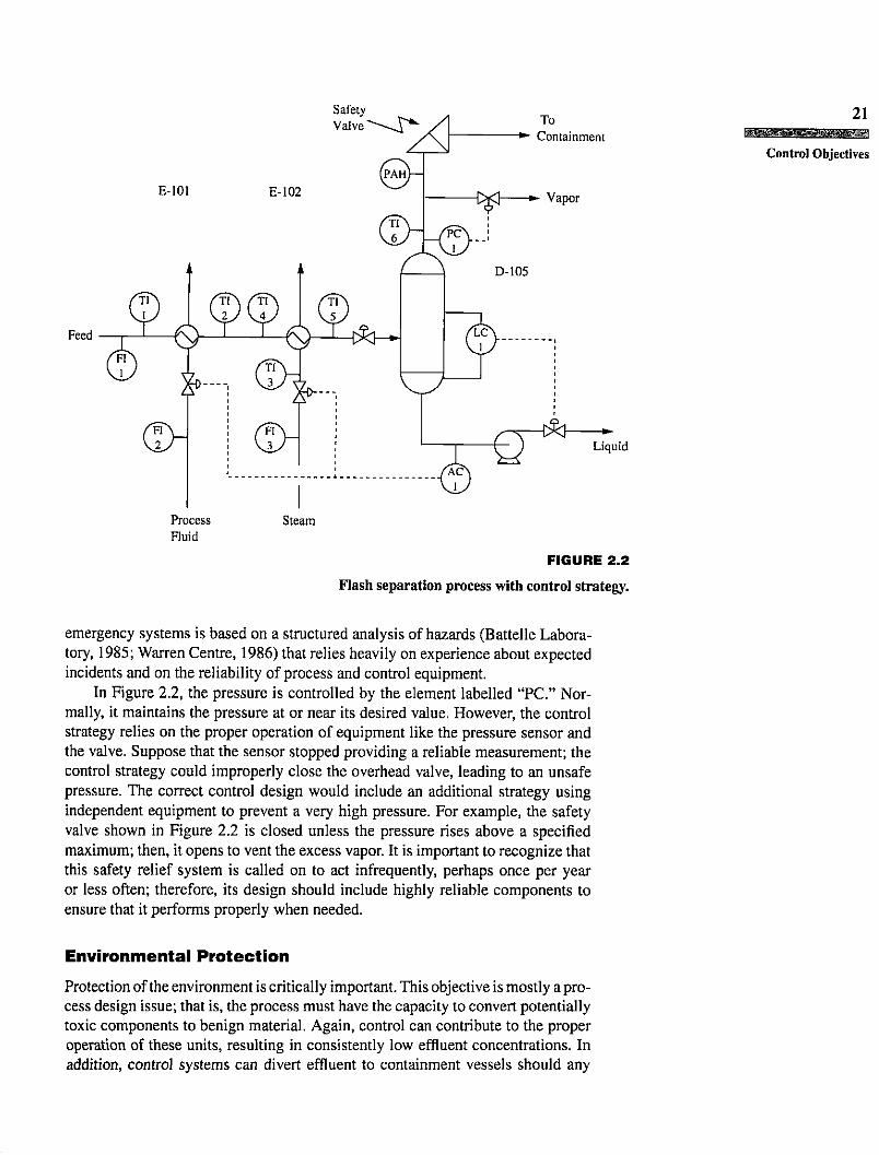
2.2 B CONTROL OBJECTIVESThe seven major categories of control objectives were introduced in Chapter 1.They are discussed in detail here, with an explanation of how each influences thecontrol design for the example process shown in Figure 2.2. The process separatestwo components based on their different vapor pressures. The liquid feed stream,consisting of components A and B, is heated by two exchangers in series. Thenthe stream flows through a valve to a vessel at a lower pressure. As a result ofthe higher temperature and lower pressure, the material forms two phases, withmost of the A in the vapor and most of the B in the liquid. The exact compositionscan be determined from an equilibrium flash calculation, which simultaneouslysolves the material, energy, and equilibrium expressions. Both streams leave thevessel for further processing, the vapor stream through the overhead line andthe liquid stream out from the bottom of the vessel. Although a simple process,the heat exchanger with flash drum provides examples of all control objectives,and this process is analyzed quantitatively with control in Chapter 24.

A control strategy is also shown in Figure 2.2. Since we have not yet studiedthe calculations used by feedback controllers, you should interpret the controller asa linkage between a measurement and a valve. Thus, you can think of the feedbackpressure control (PC) system as a system that measures the pressure and maintainsthe pressure close to its desired value by adjusting the opening of the valve in theoverhead vapor pipe. The type of control calculation, which will be covered indepth in later chapters, is not critical for the discussions in this chapter.

SafetyThe safety of people in the plant and in the surrounding community is of paramountimportance. While no human activity is without risk, the typical goal is that workingat an industrial plant should involve much less risk than any other activity in aperson's life. No compromise with sound equipment and control safety practicesis acceptable.

Plants are designed to operate safely at expected temperatures and pressures;however, improper operation can lead to equipment failure and release of potentially hazardous materials. Therefore, the process control strategies contribute tothe overall plant safety by maintaining key variables near their desired values.Since these control strategies are important, they are automated to ensure rapidand complete implementation. In Figure 2.2, the equipment could operate at highpressures under normal conditions. If the pressure were allowed to increase toofar beyond the normal value, the vessel might burst, resulting in injuries or death.Therefore, the control strategy includes a controller labelled "PC-1" that controlsthe pressure by adjusting the valve position (i.e., percent opening) in the vapor line.

Another consideration in plant safety is the proper response to major incidents,such as equipment failures and excursions of variables outside of their acceptablebounds. Feedback strategies cannot guarantee safe operation; a very large disturbance could lead to an unsafe condition. Therefore, an additional layer of control,termed an emergency system, is applied to enforce bounds on key variables. Typically, this layer involves either safely diverting the flow of material or shuttingdown the process when unacceptable conditions occur. The control strategies areusually not complicated; for example, an emergency control might stop the feedto a vessel when the liquid level is nearly overflowing. Proper design of these

SafetyValve To

Containment21

E-101 E-102(pah)—

Control Objectives

©--tfv-i* # - + Vapor

D-105

Feed

Liquid

ProcessFluid

Steam

FIGURE 2.2Flash separation process with control strategy.

emergency systems is based on a structured analysis of hazards (Battelle Laboratory, 1985; Warren Centre, 1986) that relies heavily on experience about expectedincidents and on the reliability of process and control equipment.

In Figure 2.2, the pressure is controlled by the element labelled "PC." Normally, it maintains the pressure at or near its desired value. However, the controlstrategy relies on the proper operation of equipment like the pressure sensor andthe valve. Suppose that the sensor stopped providing a reliable measurement; thecontrol strategy could improperly close the overhead valve, leading to an unsafepressure. The correct control design would include an additional strategy usingindependent equipment to prevent a very high pressure. For example, the safetyvalve shown in Figure 2.2 is closed unless the pressure rises above a specifiedmaximum; then, it opens to vent the excess vapor. It is important to recognize thatthis safety relief system is called on to act infrequently, perhaps once per yearor less often; therefore, its design should include highly reliable components toensure that it performs properly when needed.

Environmental ProtectionProtection of the environment is critically important. This objective is mostly a process design issue; that is, the process must have the capacity to convert potentiallytoxic components to benign material. Again, control can contribute to the properoperation of these units, resulting in consistently low effluent concentrations. Inaddition, control systems can divert effluent to containment vessels should any

22

CHAPTER 2Control Objectivesand Benefits

extreme disturbance occur. The stored material could be processed at a later timewhen normal operation has been restored.

In Figure 2.2, the environment is protected by containing the material withinthe process equipment. Note that the safety release system directs the material forcontainment and subsequent "neutralization," which could involve recycling to theprocess or combusting to benign compounds. For example, a release system mightdivert a gaseous hydrocarbon to a flare for combustion, and it might divert a water-based stream to a holding pond for subsequent purification through biologicaltreatment before release to a water system.

Equipment ProtectionMuch of the equipment in a plant is expensive and difficult to replace withoutcostly delays. Therefore, operating conditions must be maintained within boundsto prevent damage. The types of control strategies for equipment protection aresimilar to those for personnel protection, that is, controls to maintain conditionsnear desired values and emergency controls to stop operation safely when theprocess reaches boundary values.

In Figure 2.2, the equipment is protected by maintaining the operating conditions within the expected temperatures and pressures. In addition, the pumpcould be damaged if no liquid were flowing through it. Therefore, the liquid levelcontroller, by ensuring a reservoir of liquid in the bottom of the vessel, protectsthe pump from damage. Additional equipment protection could be provided byadding an emergency controller that would shut off the pump motor when thelevel decreased below a specified value.

Smooth Operation and Production RateA chemical plant includes a complex network of interacting processes; thus, thesmooth operation of a process is desirable, because it results in few disturbances toall integrated units. Naturally, key variables in streams leaving the process shouldbe maintained close to their desired values (i.e., with small variation) to preventdisturbances to downstream units. In Figure 2.2, the liquid from the vessel bottomsis processed by downstream equipment. The control strategy can be designed tomake slow, smooth changes to the liquid flow. Naturally, the liquid level will notremain constant, but it is not required to be constant; the level must only remainwithin specified limits. By the use of this control design, the downstream unitswould experience fewer disturbances, and the overall plant would perform better.

There are additional ways for upsets to be propagated in an integrated plant.For example, when the control strategy increases the steam flow to heat exchangerE-102, another unit in the plant must respond by generating more steam. Clearly,smooth manipulations of the steam flow require slow adjustments in the boileroperation and better overall plant operation. Therefore, we are interested in boththe controlled variables and the manipulated variables. Ideally, we would like tohave tight regulation of the controlled variables and slow, smooth adjustment ofthe manipulated variables. As we will see, this is not usually possible, and somecompromise is required.

People who are operating a plant want a simple method for maintaining theproduction rate at the desired value. We will include the important production rate

goal in this control objective. For the flash process in Figure 2.2, the natural methodfor achieving the desired production rate is to adjust the feed valve located beforethe flash drum so that the feed flow rate F\ has the desired value.

Product QualityThe final products from the plant must meet demanding quality specifications setby purchasers. The specifications may be expressed as compositions (e.g., percentof each component), physical properties (e.g., density), performance properties(e.g., octane number or tensile strength), or a combination of all three. Processcontrol contributes to good plant operation by maintaining the operating conditions required for excellent product quality. Improving product quality control is amajor economic factor in the application of digital computers and advanced controlalgorithms for automation in the process industries.

In Figure 2.2, the amount of component A, the material with the higher vaporpressure, is to be controlled in the liquid stream. Based on our knowledge ofthermodynamics, we know that this value can be controlled by adjusting the flashtemperature or, equivalently, the heat exchanged. Therefore, a control strategywould be designed to measure the composition in real time and adjust the heatingmedium flows that exchange heat with the feed.

Profit

Naturally, the typical goal of the plant is to return a profit. In the case of a utility suchas water purification, in which no income from sales is involved, the equivalentgoal is to provide the product at lowest cost. Before achieving the profit-orientedgoal, selected independent variables are adjusted to satisfy the first five higher-priority control objectives. Often, some independent operating variables are notspecified after the higher objectives (that is, including product quality but exceptingprofit) have been satisfied. When additional variables (degrees of freedom) exist,the control strategy can increase profit while satisfying all other objectives.

In Figure 2.2 all other control objectives can be satisfied by using exchangerE-101, exchanger E-102, or a combination of the two, to heat the inlet stream.Therefore, the control strategy can select the correct exchanger based on the costof the two heating fluids. For example, if the process fluid used in E-101 were lesscostly, the control strategy would use the process stream for heating preferentiallyand use steam only when required for additional heating. How the control strategy would implement this policy, based on a selection hierarchy defined by theengineer, is covered in Chapter 22.

Monitoring and DiagnosisComplex chemical plants require monitoring and diagnosis by people as well asexcellent automation. Plant control and computing systems generally provide monitoring features for two sets of people who perform two different functions: (1) theimmediate safety and operation of the plant, usually monitored by plant operators,and (2) the long-term plant performance analysis, monitored by supervisors andengineers.

The plant operators require very rapid information so that they can ensure thatthe plant conditions remain within acceptable bounds. If undesirable situations

24

CHAPTER 2Control Objectivesand Benefits

Time

HFC-1 TI-1 PC-1 LC-1FIGURE 2.3

Bar displaywith desiredvaluesindicated

Examples of displays presented to aprocess operator.

occur—or, one hopes, before they occur—the operator is responsible for rapidrecognition and intervention to restore acceptable performance. While much ofthis routine work is automated, the people are present to address complex issuesthat are difficult to automate, perhaps requiring special information not readilyavailable to the computing system. Since the person may be responsible for a plantsection with hundreds of measured variables, excellent displays are required. Theseare usually in the form of trend plots of several associated variables versus timeand of indicators in bar-chart form for easy identification of normal and abnormaloperation. Examples are shown in Figure 2.3.

Since the person cannot monitor all variables simultaneously, the control system includes an alarm feature, which draws the operator's attention to variablesthat are near limiting values selected to indicate serious maloperation. For example, a high pressure in the flash separator drum is undesirable and would at theleast result in the safety valve opening, which is not desirable, because it divertsmaterial and results in lost profit and because it may not always reclose tightly.Thus, the system in Figure 2.2 has a high-pressure alarm, PAH. If the alarm is activated, the operator might reduce the flows to the heat exchanger or of the feed toreduce pressure. This operator action might cause a violation of product specifications; however, maintaining the pressure within safe limits is more important thanproduct quality. Every measured variable in a plant must be analyzed to determinewhether an alarm should be associated with it and, if so, the proper value for thealarm limit.

Another group of people monitors the longer-range performance of the plantto identify opportunities for improvement and causes for poor operation. Usually,a substantial sample of data, involving a long time period, is used in this analysis,so that the effects of minor fluctuations are averaged out. Monitoring involvesimportant measured and calculated variables, including equipment performances(e.g., heat transfer coefficients) and process performances (e.g., reactor yields andmaterial balances). In the example flash process, the energy consumption would bemonitored. An example trend of some key variables is given in Figure 2.4, whichshows that the ratio of expensive to inexpensive heating source had an increasingtrend. If the feed flow and composition did not vary significantly, one might suspect

TC- lFlash

Time (many weeks)FIGURE 2.4

Example of long-term data, showing the increased use ofexpensive steam in the flash process.

that the heat transfer coefficient in the first heat exchanger, E-101, was decreasingdue to fouling. Careful monitoring would identify the problem and enable theengineer to decide when to remove the heat exchanger temporarily for mechanicalcleaning to restore a high heat transfer coefficient.

Previously, this monitoring was performed by hand calculations, which wasa tedious and inefficient method. Now, the data can be collected, processed if additional calculations are needed, and reported using digital computers. This combination of ease and reliability has greatly improved the monitoring of chemicalprocess plants.

Note that both types of monitoring—the rapid display and the slower processanalysis—require people to make and implement decisions. This is another form offeedback control involving personnel, sometimes referred to as having "a personin the loop," with the "loop" being the feedback control loop. While we willconcentrate on the automated feedback system in a plant, we must never forget thatmany of the important decisions in plant operation that contribute to longer-termsafety and profitability are based on monitoring and diagnosis and implementedby people "manually."

Therefore,

All seven categories of control objectives must be achieved simultaneously; failureto do so leads to unprofitable or, worse, dangerous plant operation.

In this section, instances of all seven goals were identified in the simple heaterand flash separator. The analysis of more complex process plants in terms of thegoals is a challenging task, enabling engineers to apply all of their chemical engineering skills. Often a team of engineers and operators, each with special experiences and insights, performs this analysis. Again, we see that control engineeringskills are needed by all chemical engineers in industrial practice.

25

Determining PlantOperating Conditions

Control Objectives

1. Safety2. Environmental Protection3. Equipment Protection4. Smooth Operation

and Production Rate5. Product Quality6. Profit7. Monitoring and Diagnosis

2.3 N DETERMINING PLANT OPERATING CONDITIONSA key factor in good plant operation is the determination of the best operatingconditions, which can be maintained within small variation by automatic controlstrategies. Therefore, setting the control objectives requires a clear understandingof how the plant operating conditions are determined. A complete study of plantobjectives requires additional mathematical methods for simulating and optimizingthe plant operation. For our purposes, we will restrict our discussion in this sectionto small systems that can be analyzed graphically.

Determining the best operating conditions can be performed in two steps.First, the region of possible operation is defined. The following are some of thefactors that limit the possible operation:

• Physical principles; for example, all concentrations > 0• Safety, environmental, and equipment protection• Equipment capacity; for example, maximum flow• Product quality

26

CHAPTER 2Control Objectivesand Benefits

The region that satisfies all bounds is termed the feasible operating region or, morecommonly, the operating window. Any operation within the operating window ispossible. Violation of some of the limits, called soft constraints, would lead topoor product quality or reduction of long-term equipment life; therefore, short-term violations of soft constraints are allowed but are to be avoided. Violation ofcritical bounds, called hard constraints, could lead to injury or major equipmentdamage; violations of hard constraints are not acceptable under any foreseeablecircumstances. The control strategy must take aggressive actions, including shutting down the plant, to prevent hard constraint violations. For both hard and softconstraints, debits are incurred for violating constraints, so the control system isdesigned to maintain operation within the operating window. While any operationwithin the window is possible and satisfies minimum plant goals, a great differencein profit can exist depending on the conditions chosen. Thus, the plant economicsmust be analyzed to determine the best operation within the window. The control strategy should be designed to maintain the plant conditions near their mostprofitable values.

The example shown in Figure 2.5 demonstrates the operating window for asimple, one-dimensional case. The example involves a fired heater (furnace) witha chemical reaction occurring as the fluid flows through the pipe or, as it is oftencalled, the coil. The temperature of the reactor must be held between minimum (noreaction) and maximum (metal damage or excessive side reactions) temperatures.When economic objectives favor increased conversion of feed, the profit functionmonotonically increases with increasing temperature; therefore, the best operationwould be at the maximum allowable temperature. However, the dynamic data showthat the temperature varies about the desired value because of disturbances such asthose in fuel composition and pressure. Therefore, the effectiveness of the controlstrategy in maximizing profit depends on reducing the variation of the temperature.A small variation means that the temperature can be operated very close to, withoutexceeding, the maximum constraint.

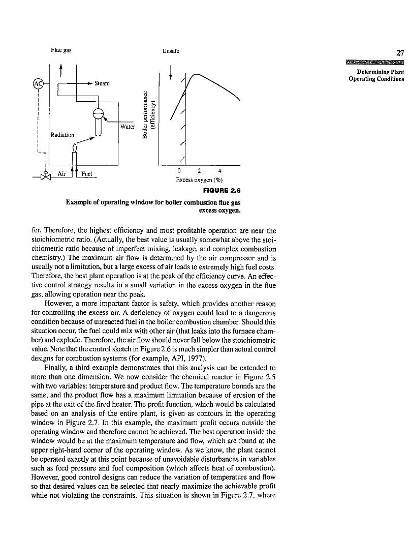
Another example is the system shown in Figure 2.6, where fuel and air aremixed and combusted to provide heat for a boiler. The ratio of fuel to air is important. Too little air (oxygen) means that some of the fuel is uncombusted andwasted, whereas excess air reduces the flame temperature and, thus, the heat trans-

Fuel

max8 \E \■<">8. \CO \<U

g sft.Temperature

FIGURE 2.5

Example of operating window for fired-heater temperature.

Flue gas Unsafe

0 2 4Excess oxygen (%)

FIGURE 2.6

Example of operating window for boiler combustion flue gasexcess oxygen.

27

Determining PlantOperating Conditions

fer. Therefore, the highest efficiency and most profitable operation are near thestoichiometric ratio. (Actually, the best value is usually somewhat above the stoichiometric ratio because of imperfect mixing, leakage, and complex combustionchemistry.) The maximum air flow is determined by the air compressor and isusually not a limitation, but a large excess of air leads to extremely high fuel costs.Therefore, the best plant operation is at the peak of the efficiency curve. An effective control strategy results in a small variation in the excess oxygen in the fluegas, allowing operation near the peak.

However, a more important factor is safety, which provides another reasonfor controlling the excess air. A deficiency of oxygen could lead to a dangerouscondition because of unreacted fuel in the boiler combustion chamber. Should thissituation occur, the fuel could mix with other air (that leaks into the furnace chamber) and explode. Therefore, the air flow should never fall below the stoichiometricvalue. Note that the control sketch in Figure 2.6 is much simpler than actual controldesigns for combustion systems (for example, API, 1977).

Finally, a third example demonstrates that this analysis can be extended tomore than one dimension. We now consider the chemical reactor in Figure 2.5with two variables: temperature and product flow. The temperature bounds are thesame, and the product flow has a maximum limitation because of erosion of thepipe at the exit of the fired heater. The profit function, which would be calculatedbased on an analysis of the entire plant, is given as contours in the operatingwindow in Figure 2.7. In this example, the maximum profit occurs outside theoperating window and therefore cannot be achieved. The best operation inside thewindow would be at the maximum temperature and flow, which are found at theupper right-hand corner of the operating window. As we know, the plant cannotbe operated exactly at this point because of unavoidable disturbances in variablessuch as feed pressure and fuel composition (which affects heat of combustion).However, good control designs can reduce the variation of temperature and flowso that desired values can be selected that nearly maximize the achievable profitwhile not violating the constraints. This situation is shown in Figure 2.7, where

28

CHAPTER 2Control Objectivesand Benefits

1i ' ii ' i• • ii ' ■

r vMax profit \

\i » »

/ • • • 3 : //

o//

U. / Targeted \/ conditions \/ ^ . -/ \

TemperatureFIGURE 2.7

Example of operating window for the feed andtemperature of a fired-heater chemical reactor.

a circle defines the variation expected about the desired values (Perkins, 1990;Narraway and Perkins, 1993). When control provides small variation, that is, acircle of small radius, the operation can be maintained closer to the best operation.

All of these examples demonstrate that

Process control improves plant performance by reducing the variation of key variables. When the variation has been reduced, the desired value of the controlledvariable can be adjusted to increase profit.

Note that simply reducing the variation does not always improve plant operation. The profit contours within the operating window must be analyzed todetermine the best operating conditions that take advantage of the reduced variation. Also, it is important to recognize that the theoretical maximum profit cannotusually be achieved because of inevitable variation due to disturbances. This situation should be included in the economic analysis of all process designs.

2.4 m BENEFITS FOR CONTROLThe previous discussion of plant operating conditions provides the basis for calculating the benefits for excellent control performance. In all of the examplesdiscussed qualitatively in the previous section, the economic benefit resulted from

reduced variation of key variables. Thus, the calculation of benefits considers theeffect of variation on plant profit. Before the method is presented, it is emphasizedthat the highest-priority control objectives—namely, safety, environmental protection, and equipment protection—are not analyzed by the method described in thissection. Although the control designs for these objectives often reduce variation,they are not selected for increasing profit but rather for providing safe, reliableplant operation.

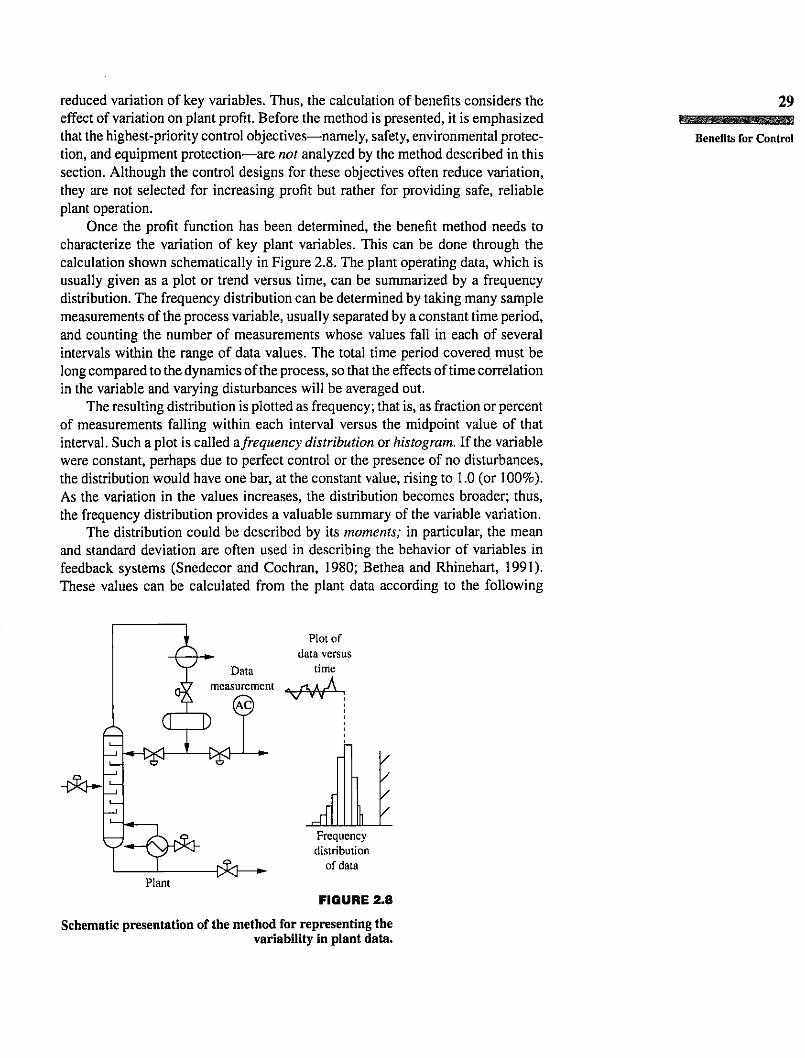
Once the profit function has been determined, the benefit method needs tocharacterize the variation of key plant variables. This can be done through thecalculation shown schematically in Figure 2.8. The plant operating data, which isusually given as a plot or trend versus time, can be summarized by a frequencydistribution. The frequency distribution can be determined by taking many samplemeasurements of the process variable, usually separated by a constant time period,and counting the number of measurements whose values fall in each of severalintervals within the range of data values. The total time period covered must belong compared to the dynamics of the process, so that the effects of time correlationin the variable and varying disturbances will be averaged out.

The resulting distribution is plotted as frequency; that is, as fraction or percentof measurements falling within each interval versus the midpoint value of thatinterval. Such a plot is called a frequency distribution or histogram. If the variablewere constant, perhaps due to perfect control or the presence of no disturbances,the distribution would have one bar, at the constant value, rising to 1.0 (or 100%).As the variation in the values increases, the distribution becomes broader; thus,the frequency distribution provides a valuable summary of the variable variation.

The distribution could be described by its moments; in particular, the meanand standard deviation are often used in describing the behavior of variables infeedback systems (Snedecor and Cochran, 1980; Bethea and Rhinehart, 1991).These values can be calculated from the plant data according to the following

29

Benefits for Control

Datameasurement

Plot ofdata versus

time

c (HZD

-c£}»* ^ ^ - t ^ 3

vvA

PlantcSd—^

JFrequencydistribution

of data

FIGURE 2.8

Schematic presentation of the method for representing thevariability in plant data.

30

CHAPTER 2Control Objectivesand Benefits

equations:

- 2 - 1 0 1 2 3Deviation from mean

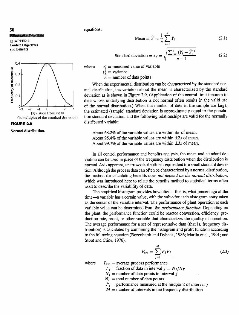
(in multiples of the standard deviation)FIGURE 2.9

Normal distribution.

1 "Mean = Y = - ^ Yt«=i

EIUM-r)2n - l

(2.1)

(2.2)Standard deviation = sy =

where F,- = measured value of variablesY = variancen = number of data points

When the experimental distribution can be characterized by the standard normal distribution, the variation about the mean is characterized by the standarddeviation as is shown in Figure 2.9. (Application of the central limit theorem todata whose underlying distribution is not normal often results in the valid useof the normal distribution.) When the number of data in the sample are large,the estimated (sample) standard deviation is approximately equal to the population standard deviation, and the following relationships are valid for the normallydistributed variable:

About 68.2% of the variable values are within ±s of mean.About 95.4% of the variable values are within ±2s of mean.About 99.7% of the variable values are within ±3s of mean.

In all control performance and benefits analysis, the mean and standard deviation can be used in place of the frequency distribution when the distribution isnormal. As is apparent, a narrow distribution is equivalent to a small standard deviation. Although the process data can often be characterized by a normal distribution,the method for calculating benefits does not depend on the normal distribution,which was introduced here to relate the benefits method to statistical terms oftenused to describe the variability of data.

The empirical histogram provides how often—that is, what percentage of thetime—a variable has a certain value, with the value for each histogram entry takenas the center of the variable interval. The performance of plant operation at eachvariable value can be determined from the performance function. Depending onthe plant, the performance function could be reactor conversion, efficiency, production rate, profit, or other variable that characterizes the quality of operation.The average performance for a set of representative data (that is, frequency distribution) is calculated by combining the histogram and profit function accordingto the following equation (Bozenhardt and Dybeck, 1986; Marlin et al., 1991; andStout and Cline, 1976).

M

P m = J 2 f j p j < 2 3 )where Pave = average process performance

Fj = fraction of data in interval j = Nj/NjNj = number of data points in interval jNt = total number of data pointsPj = performance measured at the midpoint of interval jM = number of intervals in the frequency distribution

Datameasurement

Plot ofdata versus

time

f * \

D&K

(U_D^ — L - ^

© W v ^

Plant { & r —

Processvariable

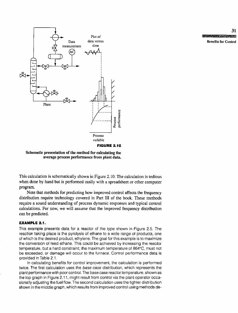
FIGURE 2.10Schematic presentation of the method for calculating the

average process performance from plant data.

31

Benefits for Control

This calculation is schematically shown in Figure 2.10. The calculation is tediouswhen done by hand but is performed easily with a spreadsheet or other computerprogram.

Note that methods for predicting how improved control affects the frequencydistribution require technology covered in Part in of the book. These methodsrequire a sound understanding of process dynamic responses and typical controlcalculations. For now, we will assume that the improved frequency distributioncan be predicted.

EXAMPLE 2.1.This example presents data for a reactor of the type shown in Figure 2.5. Thereaction taking place is the pyrolysis of ethane to a wide range of products, oneof which is the desired product, ethylene. The goal for this example is to maximizethe conversion of feed ethane. This could be achieved by increasing the reactortemperature, but a hard constraint, the maximum temperature of 864°C, must notbe exceeded, or damage will occur to the furnace. Control performance data isprovided in Table 2.1.

In calculating benefits for control improvement, the calculation is performedtwice. The first calculation uses the base case distribution, which represents theplant performance with poor control. The base case reactor temperature, shown asthe top graph in Figure 2.11, might result from control via the plant operator occasionally adjusting the fuel flow. The second calculation uses the tighter distributionshown in the middle graph, which results from improved control using methods de-

32

CHAPTER 2Control Objectivesand Benefits

scribed in Parts III and IV. The process performance correlation, which is requiredto relate the temperature to conversion, is given in the bottom graph. The data forthe graphs, along with the calculations for the averages, are given in Table 2.1.

The difference between the two average performances, a conversion increaseof 4.4 percent, is the benefit for improved control. Note that the benefit is achievedby reducing the variance and increasing the average temperature. Both are required in this example; simply reducing variance with the same mean would notbe a worthwhile achievement! Naturally, this benefit must be related to dollarsand compared with the costs for equipment and personnel time when decidingwhether this investment is justified. The economic benefit would be calculated asfollows:

Aprofit = (feed flow) (A conversion) ($/kg products) (2.4)In a typical ethylene plant, the benefits for even a small increase in conversionwould be much greater than the costs. Additional benefits would result from fewerdisturbances to downstream units and longer operating life of the fired heater dueto reduced thermal stress.

EXAMPLE 2.2.A second example is given for the boiler excess oxygen shown in Figure 2.6. Thediscussion in the previous section demonstrated that the profit is maximized whenthe excess oxygen is maintained slightly above the stoichiometric ratio, wherethe efficiency is at its maximum. Again, the process performance function, hereefficiency, is used to evaluate each operating value, and frequency distributionsare used to characterize the variation in performance.

The performance is calculated for the base case and an improved controlcase, and the benefit is calculated as shown in Figure 2.12 for an example with

TABLE 2.1Frequency data for Example 2.1

Data withInitial data improved control

Temperature midpoint Conversion P.-(°C) (%) *7 Pj*Fj F j P,*F,842 50 0 0 0 0844 51 0.0666 3.4 0 0846 52 0.111 5.778 0 0848 53 0.111 5.889 0 0850 54 0.156 8.4 0 0852 55 0.244 13.44 0 0854 56 0.133 7.467 0 0856 57 0.111 6.333 0 0858 58 0.044 2.578 0.25 14.5860 59 0.022 1.311 0.50 29.5862 60 0 0 0.25 15

Average conversion (%) =■ E P j * F j = 54.6 59

0.25 0.25

0.20

.2 0.15

e 0.10

fc 0.05

0.00842 846 850 854 858 862

Temperature

0.00

33

0.25 1.25 2.25 3.25 4.25Oxygen (mol %)

5.25

0,0.0,0,0.0,0.0.

£ 0.0.0.

co•aoi=>>acu3

0.500.450.400.350.300.250.200.150.100.05

842 846 850 854 858 862Temperature

0.00

Hm1Ii i111ii 1111§i 1M i l l in i i i i

0.25 1.25 2.25 3.25 4.25Oxygen (mol %)

5.25

0.60

oo

•s

842 846 850 854 858 862Temperature

FIGURE 2.11Data for Example 2.1 in which the

benefits of reduced variation and closerapproach to the maximum temperature

limit in a chemical reactor are calculated.

0.25 5.251.25 2.25 3.25 4.25Oxygen (mol %)

FIGURE 2.12Data for Example 2.2 in which the

benefits of reducing the variation ofexcess oxygen in boiler flue gas are

calculated.

Benefits for Control

realistic data. The data for the graphs, along with the calculations for the averages,are given in Table 2.2. The average efficiency increased by almost 1 percent withbetter control and would be related to profit as follows:

Aprofit = (A efficiency/100) (steam flow) (A#vap) ($/energy) (2.5)This improvement would result in fuel savings worth tens of thousands of dollarsper year in a typical industrial boiler. In this case, the average of the processvariable (excess oxygen) is the same for the initial and improved operations, because the improvement is due entirely to the reduction in the variance of the excess

34

CHAPTER 2Control Objectivesand Benefits

oxygen. The difference between the chemical reactor and the boiler results fromthe different process performance curves. Note that the improved control case hasits desired value at an excess oxygen value slightly greater than where the maximum profit occurs, so that the chance of a dangerous condition is negligibly small.

A few important assumptions in this benefits calculation method may not beobvious, so they are discussed here. First, the frequency distributions can neverbe guaranteed to remain within the operating window. If a large enough dataset were collected, some data would be outside of the operating window due toinfrequent, large disturbances. Therefore, some small probability of exceeding theconstraints always exists and must be accepted. For soft constraints, it is commonto select an average value so that no more than a few percent of the data exceeds theconstraint; often the target is two standard deviations from the limit. For importanthard constraints, an average much farther from the constraint can be selected, sincethe emergency system will activate each time the system reaches a boundary.

A second assumption concerns the mixing of steady-state and dynamic relationships. Remember that the process performance function is developed fromsteady-state analysis. The frequency distribution is calculated from plant data,which is inherently dynamic. Therefore, the two correlations cannot strictly beused together, as they are in equation (2.3). The difficulty is circumvented if theplant is assumed to have operated at quasi-steady state at each data point, thenvaried to the next quasi-steady state for the subsequent data point. When thisassumption is valid, the plant data is essentially from a series of steady-state operations, and equation (2.3) is valid, because all data and correlations are consistentlysteady-state.

TABLE 2.2

Frequency data for Example 2.2Data with

Ini t ia l data improved contro lExcess oxygen midpoint Boiler efficiency Pj

(mol fract ion) (%) Fj P, * F, Fj P,*F j0.25 83.88 0 0 0 00.75 85.70 0 0 0 01.25 86.85 0.04 3.47 0 01.75 87.50 0.12 10.50 0.250 2.192.25 87.70 0.24 21.05 0.475 41.662.75 87.54 0.12 10.50 0.475 41.583.25 87.10 0.20 17.42 0.025 2.183.75 86.48 0.04 3.46 0 04.25 85.76 0.08 6.86 0 04.75 85.02 0.04 3.40 0 05.25 84.36 0.08 6.75 0 05.75 83.86 0.04 3.35 0 0

Average efficiency (%) =■ Y , P j *Fy = 86.77 87.70I^MM#^ftS»^#^ff.tgM^g))EJW^

Third, the approach is valid for modifying the behavior of one process variable,with all other variables unchanged. If many control strategies are to be evaluated,the interaction among them must be considered. The alterations to the proceduredepend on the specific plant considered but would normally require a model of theintegrated plant.

35

Importance of ControlEngineering

The analysis method presented in this section demonstrates that information on thevariability of key variables is required for evaluating the performance of a process-average values of process variables are not adequate.

The method explained in this section clearly demonstrates the importance ofunderstanding the goals of the plant prior to evaluating and designing the controlstrategies. It also shows the importance of reducing the variation in achieving goodplant operation and is a practical way to perform economic evaluations of potentialinvestments.

2.5 n IMPORTANCE OF CONTROL ENGINEERINGGood control performance yields substantial benefits for safe and profitable plantoperation. By applying the process control principles in this book, the engineerwill be able to design plants and control strategies that achieve the control objectives. Recapitulating the material in Chapter 1, control engineering facilitates goodcontrol by ensuring that the following criteria are satisfied.

Control Is PossibleThe plant must be designed with control strategies in mind so that the appropriatemeasurements and manipulated variables exist. Control of the composition of theliquid product from the flash drum in Figure 2.2 requires the flexibility to adjustthe valves in the heating streams. Even if the valve can be adjusted, the total heatexchanger areas and utility flows must be large enough to satisfy the demands ofthe flash process. Thus, the chemical engineer is responsible for ensuring that theprocess equipment and control equipment provide sufficient flexibility.

The Plant Is Easy to Control

Clearly, reduction in variation is desired. Typically, plants that are subject to fewdisturbances, due to inventory (buffer) between the disturbance and the controlledvariable, are easier to control. Unfortunately, this is contradictory to many moderndesigns, which include energy-saving heat integration schemes and reduced plantinventories. Therefore, the dynamic analysis of such designs is important to determine how much (undesired) variance results from the (desired) lower capital costsand higher steady-state efficiency. Also, the plant should be "responsive"; that is,the dynamics between the manipulated and controlled variables should be fast—thefaster the better. Plant design can influence this important factor substantially.

36

CHAPTER 2Control Objectivesand Benefits

Proper Control Calculations Are Used

Properly designed control calculations can improve the control performance byreducing the variation of the controlled variable. Some of the desired characteristicsfor these calculations are simplicity, generality, reliability, and flexibility. The basiccontrol algorithm is introduced in Chapter 8.

Control Equipment Is Properly Selected

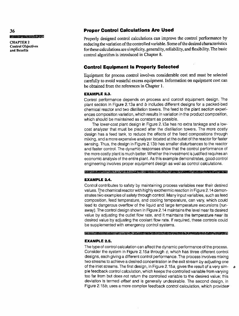
Equipment for process control involves considerable cost and must be selectedcarefully to avoid wasteful excess equipment. Information on equipment cost canbe obtained from the references in Chapter 1.EXAMPLE 2.3.Control performance depends on process and control equipment design. Theplant section in Figure 2.13a and b includes different designs for a packed-bedchemical reactor and two distillation towers. The feed to the plant section experiences composition variation, which results in variation in the product composition,which should be maintained as constant as possible.

The lower-cost plant design in Figure 2.13a has no extra tankage and a low-cost analyzer that must be placed after the distillation towers. The more costlydesign has a feed tank, to reduce the effects of the feed compositions throughmixing, and a more expensive analyzer located at the outlet of the reactor for fastersensing. Thus, the design in Figure 2.13b has smaller disturbances to the reactorand faster control. The dynamic responses show that the control performance ofthe more costly plant is much better. Whether the investment is justified requires aneconomic analysis of the entire plant. As this example demonstrates, good controlengineering involves proper equipment design as well as control calculations.

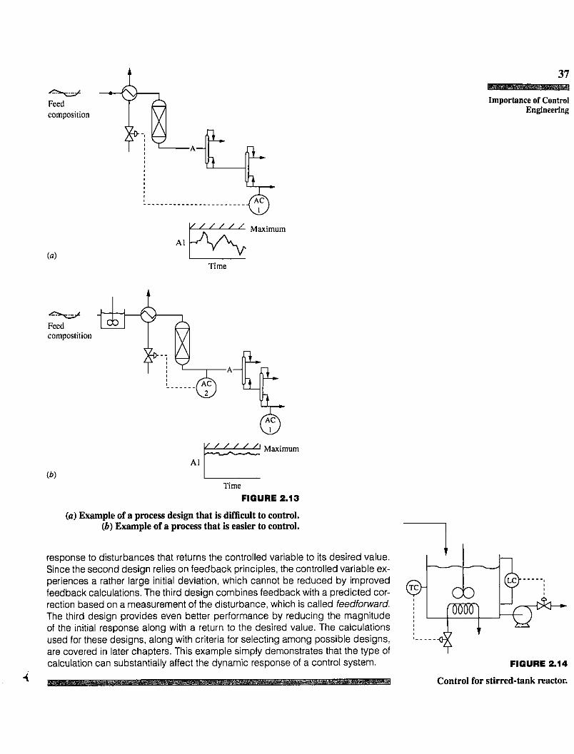
EXAMPLE 2.4.Control contributes to safety by maintaining process variables near their desiredvalues. The chemical reactor with highly exothermic reaction in Figure 2.14 demonstrates two examples of safety through control. Many input variables, such as feedcomposition, feed temperature, and cooling temperature, can vary, which couldlead to dangerous overflow of the liquid and large temperature excursions (runaway). The control design shown in Figure 2.14 maintains the level near its desiredvalue by adjusting the outlet flow rate, and it maintains the temperature near itsdesired value by adjusting the coolant flow rate. If required, these controls couldbe supplemented with emergency control systems.

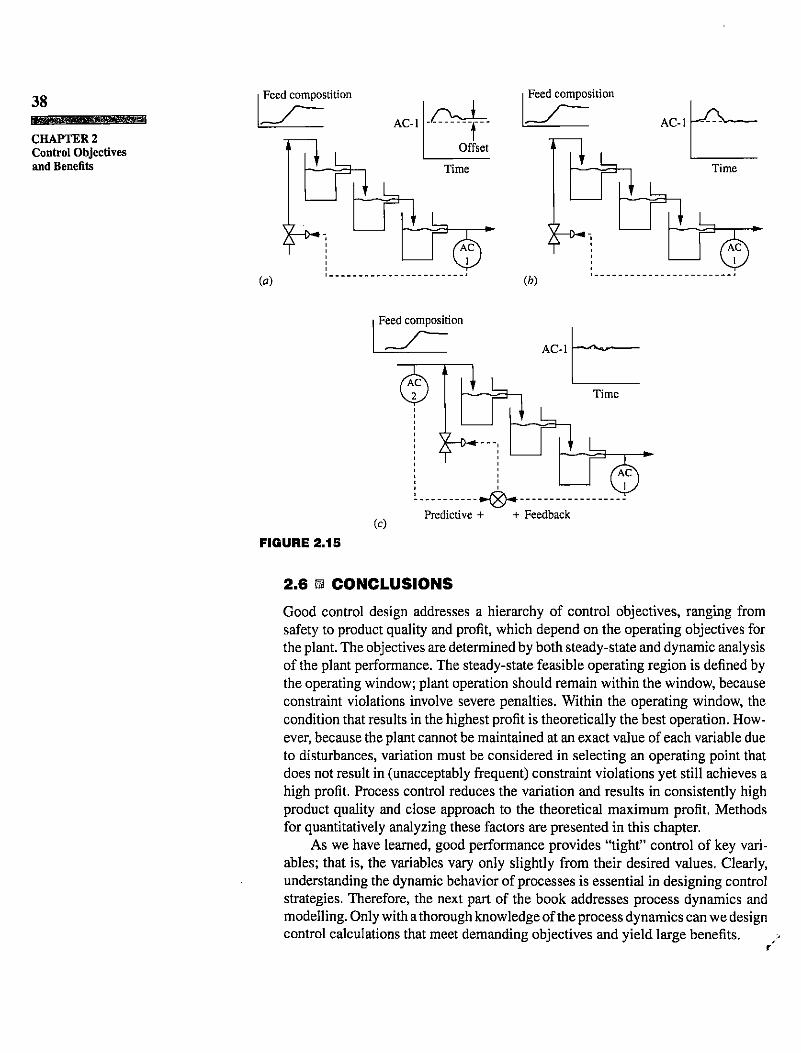
EXAMPLE 2.5.The type of control calculation can affect the dynamic performance of the process.Consider the system in Figure 2.15a through c, which has three different controldesigns, each giving a different control performance. The process involves mixingtwo streams to achieve a desired concentration in the exit stream by adjusting oneof the inlet streams. The first design, in Figure 2.15a, gives the result of a very simple feedback control calculation, which keeps the controlled variable from varyingtoo far from but does not return the controlled variable to the desired value; thisdeviation is termed offset and is generally undesirable. The second design, inFigure 2.156, uses a more complex feedback control calculation, which provides*'

Feedcomposition

■A—f t *

3 _

37

Importance of ControlEngineering

V / / / / /Al

(a)

Maximum

Time

Feedcompostition

f t *A—

a. f t *

1

^ ^ ^^ / </| MaximumAl

(6)Time

FIGURE 2.13

(a) Example of a process design that is difficult to control.(b) Example of a process that is easier to control.

response to disturbances that returns the controlled variable to its desired value.Since the second design relies on feedback principles, the controlled variable experiences a rather large initial deviation, which cannot be reduced by improvedfeedback calculations. The third design combines feedback with a predicted correction based on a measurement of the disturbance, which is called feedforward.The third design provides even better performance by reducing the magnitudeof the initial response along with a return to the desired value. The calculationsused for these designs, along with criteria for selecting among possible designs,are covered in later chapters. This example simply demonstrates that the type ofcalculation can substantially affect the dynamic response of a control system.

(rc)- OD

4C&1—-

FIGURE 2.14Control for stirred-tank reactor.

38

CHAPTER 2Control Objectivesand Benefits

Feed compostition

AC-1n u Offset

f°~-

Time

\Ua

(«)

li-U

Feed composition

AC-1n u Time

£-D-i(6)

u

Feed composition

(c)FIGURE 2.15

^ D * .

uAC-1

UTime

kHgH

Predictive + + Feedback

2.6 m CONCLUSIONSGood control design addresses a hierarchy of control objectives, ranging fromsafety to product quality and profit, which depend on the operating objectives forthe plant. The objectives are determined by both steady-state and dynamic analysisof the plant performance. The steady-state feasible operating region is defined bythe operating window; plant operation should remain within the window, becauseconstraint violations involve severe penalties. Within the operating window, thecondition that results in the highest profit is theoretically the best operation. However, because the plant cannot be maintained at an exact value of each variable dueto disturbances, variation must be considered in selecting an operating point thatdoes not result in (unacceptably frequent) constraint violations yet still achieves ahigh profit. Process control reduces the variation and results in consistently highproduct quality and close approach to the theoretical maximum profit. Methodsfor quantitatively analyzing these factors are presented in this chapter.

As we have learned, good performance provides "tight" control of key variables; that is, the variables vary only slightly from their desired values. Clearly,understanding the dynamic behavior of processes is essential in designing controlstrategies. Therefore, the next part of the book addresses process dynamics andmodelling. Only with a thorough knowledge of the process dynamics can we designcontrol calculations that meet demanding objectives and yield large benefits.

39REFERENCESAPI, American Petroleum Institute Recommended Practice 550 (2nd ed.),

Manual on Installation of Refining Instruments and Control Systems: Additional ResourcesFired Heaters and Inert Gas Generators, API, Washington, DC, 1977.

Bethea, R., and R. Rhinehart, Applied Engineering Statistics, Marcel Dekker,New York, 1991.

Battelle Laboratory, Guidelines for Hazard Evaluation Procedures, AmericanInstitute for Chemical Engineering (AIChE), New York, 1985.

Bozenhardt, H., and M. Dybeck, "Estimating Savings from Upgrading ProcessControl," Chem. Engr., 99-102 (Feb. 3, 1986).

Gorzinski, E., "Development of Alkylation Process Model," European Confion Chem. Eng„ 1983, pp. 1.89-1.96.

Marlin, T., J. Perkins, G. Barton, and M. Brisk, "Process Control Benefits,A Report on a Joint Industry-University Study," Process Control, I, pp.68-83(1991).

Narraway, L., and J. Perkins, "Selection of Process Control Structure Basedon Linear Dynamic Economics," IEC Res., 32, pp. 2681-2692 (1993).

Perkins, J., "Interactions between Process Design and Process Control," inJ. Rijnsdorp et al. (ed.), DYCORD+ 1990, International Federation ofAutomatic Control, Pergamon Press, Maastricht, Netherlands, pp. 195-203 (1989).

Snedecor, G., and W. Cochran, Statistical Methods, Iowa State UniversityPress, Ames, IA, 1980.

Stout, T., and R. Cline, "Control System Justification," Instrument. Tech., Sept.1976,51-58.

Warren Centre, Major Industrial Hazards, Technical Papers, University ofSydney, Australia, 1986.

ADDITIONAL RESOURCESThe following references provide guidance on performing benefits studies in industrial plants, and Marlin et al. (1987) gives details on studies in seven industrialplants.

Marlin, T., J. Perkins, G. Barton, and M. Brisk, Advanced Process ControlApplications—Opportunities and Benefits, Instrument Society of America, Research Triangle Park, NC, 1987.

Shunta, J., Achieving World Class Manufacturing through Process Control,Prentice-Hall PTR, Englewood Cliffs, NJ, 1995.

For further examples of operating windows and how they are used in setting processoperating policies, see

Arkun, Y, and M. Morari, "Studies in the Synthesis of Control Structures forChemical Processes, Part IV," AIChE J., 26, 975-991 (1980).

Fisher, W, M. Doherty, and J. Douglas, "The Interface between Design andControl," IEC Res., 27, 597-615 (1988).

40

CHAPTER 2Control Objectivesand Benefits

Maarleveld, A., and J. Rijnsdorp, "Constraint Control in Distillation Columns,"Automatica, 6, 51-58 (1970).

Morari, M., Y Arkun, and G. Stephanopoulos, "Studies in the Synthesis ofControl Structures for Chemical Processes, Part HI," AIChE J., 26, 220(1980).

Roffel, B., and H. Fontien, "Constraint Control of Distillation Processes,"Chem. Eng. ScL, 34,1007-1018 (1979).

These questions provide exercises in relating process variability to performance.Much of the remainder of the book addresses how process control can reduce thevariability of key variables.

QUESTIONS2.1. For each of the following processes, identify at least one control objective in

each of the seven categories introduced in Section 2.2. Describe a feedbackapproach appropriate for achieving each objective.(a) The reactor-separator system in Figure 1.8(b) The boiler in Figure 14.17(c) The distillation column in Figure 15.18(d) The fired heater in Figure 17.17

2.2. The best distribution of variable values depends strongly on the performance function of the process. Three different performance functions aregiven in Figure Q2.2. In each case, the average value of the variable (xave)must remain at the specified value, although the distribution around the average is not specified. The performance function, P, can be assumed to be

ATAverageProcess variable

FIGURE Q2.2

AverageProcess variable

AverageProcess variable

a quadratic function of the variable, x, in every segment of the distribution.

P,=a-\-b (Xj - xave) + c (Xi - *ave)2

For each of the cases in Figure Q2.2, discuss the relationship between thedistribution and the average profit, and determine the distribution that willmaximize the average performance function. Provide quantitative justification for your result.

2.3. The fired heater example in Figure 2.11 had a hard constraint.(a) Sketch the performance function for this situation, including the per

formance when violations occur, on the figure.(b) Assume that the distribution of the temperature would have 0.005 frac

tion of its operation exceeding the limit of 864°C and that each timethe limit is exceeded, the plant incurs a cost of $1,000 to restart theequipment. Can you calculate the total cost per year for exceeding thelimit?

(c) Make any additional assumptions and complete the calculation.

2.4. Sometimes there is no active hard constraint. Assume that the fired heaterin Figure 2.11 has no hard constraint, but that a side reaction formingundesired products begins to occur significantly at 850°C. This side reactionhas an activation energy with larger magnitude than the product reaction.Sketch the shape of the performance function for this situation. How wouldyou determine the best desired (average) value of the temperature and thebest temperature distribution?

2.5. Sometimes engineers use a shortcut method for determining the averageprocess performance. In this shortcut, the average variable value is used,rather than the full distribution, in calculating the performance. Discuss theassumptions implicit in this shortcut and when it is and is not appropriate.

2.6. A chemical plant produces vinyl chloride monomer for subsequent production of polyvinyl chloride. This plant can sell all monomer it can producewithin quality specifications. Analysis indicates that the plant can produce175 tons/day of monomer with perfect operation. A two-month productionrecord is given in Figure Q2.6. Calculate the profit lost by not operatingat the highest value possible. Discuss why the plant production might notalways be at the highest possible value.

2.7. A blending process, shown in Figure Q2.7, mixes component A into astream. The objective is to maximize the amount of A in the stream withoutexceeding the upper limit of the concentration of A, which is 2.2 mole/m3.The current operation is "open-loop," with the operator occasionally looking at the analyzer value and changing the flow of A. The flow during theperiod that the data was collected was essentially constant at 1053 m3/h.How much more A could have been blended into the stream with perfectcontrol, that is, if the concentration of A had been maintained exactly at itsmaximum? What would be the improvement if the new distribution werenormal with a standard deviation of 0.075 mole/m3?

42

CHAPTER 2Control Objectivesand Benefits

167.00166.00

FIGURE Q2.6Time (months)

(Reprinted by permission. Copyright ©1987, InstrumentSociety of America. From Marlin, T. et al., AdvancedProcess Control Applications—Opportunities and Benefits,ISA, 1987.)

Pure A

Solvent Blended"stream

Historical data 1'//

■ i.l~i f

■ i 1 IV fi'-*\ /

,"T1 1 ty ^1''■• •: t| f

i:-"''\ii 1

ij'. 'H1 f-"'' :' 1

'■";< I1

,-=•:■','1

?

0.30.25

fr 0.2§ 0.15I£ o.i

0.050

1.5 1.6 1.7 1.8 1.9 2.0 2.1Concentration of A in blend, moles/m3

FIGURE Q2.7

,—Limitingvalue

2.8. The performance function for a distillation tower is given in Figure Q2.8in terms of lost profit from the best operation as a function of the bottomsimpurity, *B (Stout and Cline, 1978). Calculate the average performancefor the four distributions (A through D) given in Table Q2.8 along withthe average and standard deviation of the concentration, x&. Discuss therelationship between the distributions and the average performance.

0.00

°" -60.00 -

-70.00

TABLE Q2.8 43

2.00 3.00 4.00Bottoms impurity, xB

6.00

FIGURE Q2.8

(Reprinted by permission. Copyright ©1976, InstrumentSociety of America. From Stout, T., and R. Cline,

"Control Systems Justification." Instr. Techn.,September 1976, pp. 51-58.)

Fraction off time al X g

XB A B C D0.25 0 0 0 00.5 0.25 0.05 0 00.75 0.50 0.05 0 01.0 0.25 0.10 0 01.5 0 0.20 0 0.3332.0 0 0.30 0 0.3333.0 0 0.20 0.25 0.3334.0 0 0.10 0.50 05.0 0 0 0.25 06.0 0 0 0 0maammmmmm^mmmmmummmmummmmam

Questions

2.9. Profit contours similar to those in Figure Q2.9 have been reported byGorzinski (1983) for a distillation tower separating normal butane andisobutane in an alkylation process for a petroleum refinery. Based on theshape of the profit contours, discuss the selection of desired values for thedistillate and bottoms impurity variables to be used in an automation strategy. (Recall that some variation about the desired values is inevitable.) Ifonly one product purity can be controlled tightly to its desired value, whichwould be the one you would select to control tightly?

P 5I 3

Profit as %of maximum

1 2 3Light key in bottoms (mole %)

FIGURE Q2.9