~AD-A277 059 - Defense Technical Information · PDF fileThis report is on a pilot study to...
70
UNCLASSIFIED * ~AD-A277 059 EAIMTU, SOME ,.f DEECEAPLCTINEF IILA RMT SOM DFECEAPPROV CATIONS OFLI CIVILANSE OT 59-W 0'1 p01
-
Upload
truongdien -
Category
Documents
-
view
218 -
download
0
Transcript of ~AD-A277 059 - Defense Technical Information · PDF fileThis report is on a pilot study to...

UNCLASSIFIED
* ~AD-A277 059 EAIMTU,
SOME ,.f DEECEAPLCTINEF IILA RMT
SOM DFECEAPPROV CATIONS OFLI CIVILANSE OT
59-W 0'1 p01

U)
JISCLAIME NO TIC!a* 0
THIS DOCUMENT IS BESTQUALITY AVAILABLE. THE COPY
FURNISHED TO DTIC CONTAINEDA SIGNIFICANT NUMBER OF
COLOR PAGES WHICH DO NOT
REPRODUCE LEGIBLY ON BLACK
AND WhITE MICROFICHE.-
*

UNCLASSIFIED
DSTOA 0A U 5T AL I A
ELECTRONICS RESEARCH LABORATORY
Information TechnologyDivision
Accesiofi For
RESEARCH REPORT NTIS C-RA-&jERL-0694-RR D T iC TA Bc
SOME DEFENCE APPLICATIONS OF CIVILIAN REMOTESENSING SATELLITE IMAGES Ey
by .2;yC35
Vittala K. Shettigara, Gordon M. Sumerling and Paul j. Whitbread Avai 0jorDist S~
SUMMARY
This report is on a pilot study to demonstrate some of the capabilities of remote sensing in00intelligence gathering. A wide variety of issues, both quantitative and qualitative ,areaddressed. SPOT satellite images were used for object classification using statistical andneural net techniques, object height determination and image resolution enhancement. Anew procedure was developed for detecting small and man-made objects in multispectralor colour images.The procedure will be presented in a separate report.
Q COMMONWEALTH OF AUSTRALIA 1993
NOV 93 COPY No.
APPROVED FOR PUBLIC RELEASE
POSTAL ADDRESS: Director, EIectminics Reseach Laboratory, PO Box 1500, Salisbury, South Australia, 510S.
UNCLASSIFIED

ERL-0694-RR UNCLASSIFIED 0 60
This work is Copyright. Apart from any fair dealing for the purpose of study, research,criticism or review, as permitted under the Copyright Act 1968, no part may be
reproduced by any process without written permission. Copyright is the responsibility
of the Director Publishing and Marketing, AGPS. Inquiries should be directed to the
Manager, AGPS Press, Australian Government Publishing Service, GPO Box 84,
Canberra ACT 2601. * *
U -S
UNCLASSIFIED
* 0 0

UNCLASSIFIED ERL-0694-RR 0
CONTENTS 0
Page No
ABBREVIATIONS ........................................................................................................... vii
I INTRODUCTION AND OBJECTIVES .................................................................. 1 0
2 ROLE OF REMOTE SENSING IN DEFENCE ......................................................... 2
3 THE STUDY AREA AND THE DATA BASE ......................................................... 3
3.1 The study area .............................................................................................. 33.2 The data base ............................................................................................... 3 •
4 PATTERN RECOGNITION ................................................................................. 13
4.1 Pattern recognition - a brief review ............................................................. 134.2 Statistical pattern recognition - which technique to use ? .................................. 144.3 Digital Pattern recognition versus aerial photo-interpretation ..................... 144.4 Robustness of common classifiers ....................................................................... 14 0
4.5 Choice of classes and training areas ................................... 164.6 Classifications using Maximum Likelihood ................................................. 19
4.6.1 Classification accuracy .................................................................. 194.6.2 Classification blunders ................................................................... 20
4.7 Classifications using Multi-Layer Perceptron .............................................. 27 274.7.1 Some notes on the application of MLPs to classification .................... 27
4.7.2 Classification Accuracy .................................................................. 31
4.8 Conclusions ................................................................................................ 32
5 OBJECT HEIGHT DETERMINATION ................................................................. 33 •5.1 Shadow - an important part of images ........................................................ 33
5.2 Sun - satellite geometry and the equations ................................................. 33
5.3 Relationship between shadow width, pixel size and intensities .................. 36
5.3.1 The role of pixel dimension ................................. ................................ 365.4 Shadow Segmentation ..................................................................................... 37 0 0
5.4.1 Choosing the threshold for delineating shadow zones ...................... 37
5.4.2 Measurement of shadow width ....................................................... 38
5.5 Result and discussion ................................................................................... 435.6 Some limitations of the technique ................................................................ 49
6 NEW IMAGE ENHANCEMENT TOOLS ................................................................... 50 0
6.1 Smooth image zooming .............................................................................. 50
6.2 Multispectral image enhancement by merging higher resolution panchromatic
data .......................................................................................................... 54
7 CONCLUSIONS .................................................................................................. 57 0
BIBLIOGRAPHY ............................................................................................................... 59
UNCLASSIFIED iii

ERL-0694-RR UNCLASSIFIED 0
FIGURES
3.1 Scanned colour aerial photograph of the study areataken on 5 Jan 1987 ................... 5
3.2 Multispectral SPOT image of the areataken on 21 April 1987. Pixel resolution 20 m .... 7
3.3 Panchromatic SPOT image of the area taken on 21 April 1987. Pixel resolution 10 m ..... 9
3.4 Digital map of the area (source AUSUG). Resolution Im approximate .................. _11
4.1 Mean spectral responses for 11 super classes with the standard deviations marked ...... 19
4.2 An illustration of the effect of mixing of two classes - light bitumen surface, such as
runways, and open fields, such as crop and pastures .............................................. 21
43 Detailed spectral profile of metallic surface and concrete theme classes ..................... 24
4.4 Result of maximum likelihood classification after sub-dividing dull metal class. The
accuracy figures are with respect to test areas. The overall accuracy of artificial
objects is 87.3% ......................................................................................................... 25
4.5 Results of ANN classification using classes selected for GMLC classifier ............... 29
5.1 End view of the sun-satellite configuration as seen during imaging .............. 34
5.2 Plan view of the sun-satellite configuration as seen during imaging ............ 35
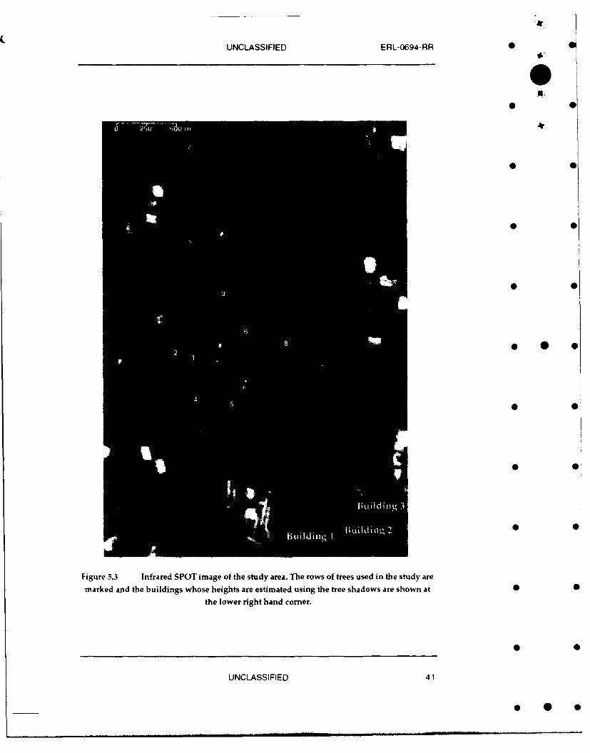
5.3 Infrared SPOT image of the study area. The rows of trees used in the study are
marked and the buildings whose heights are estimated using the tree shadows are
shown at the lower right hand com er .................................................................... 41
5.4 Shadow zones, shown as polygons, delineated using the thresholding procedure on
the infrared and the panchromatic bands ............................................................ 43
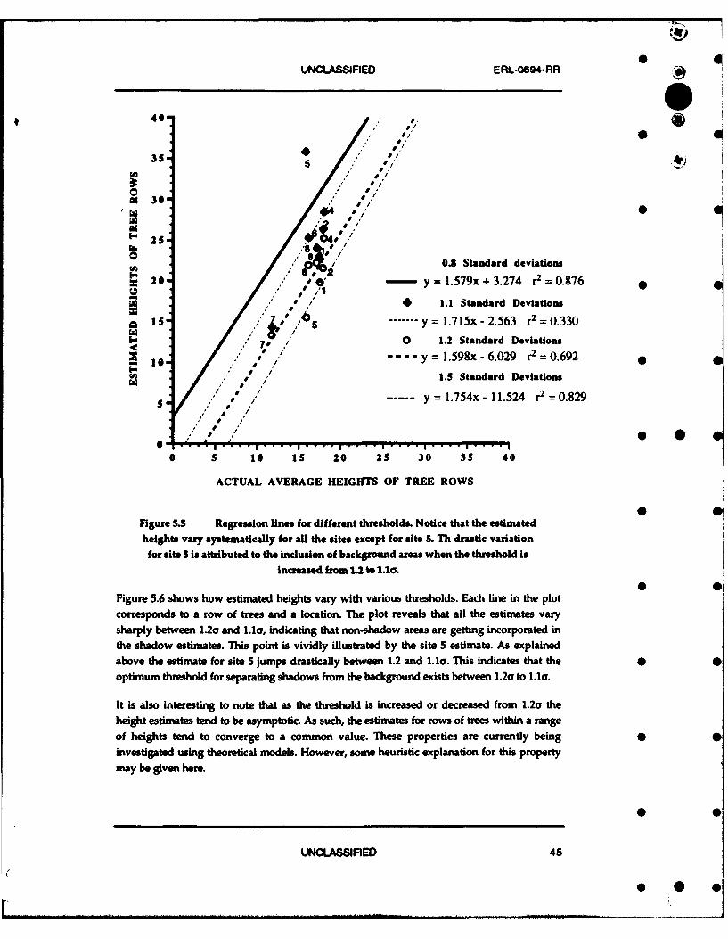
5.5 Regression lines for different thresholds. Notice that the estimated heights vary
systematically for all the sites except for site 5. Th drastic variation for site 5 is
attributed to the inclusion of background areas when the threshold is increased
from 1.2 to 1.1s ..................................................................................................... 45
5.6 Variation of estimated tree height with threshold. Notice that the estimated
heights converge at two extreme thresholds. Also the variation gradient is maximum
betw een 1.2 and 1.1s ............................................................................................. 46
5.7 A sketch of intensity variation across shadow boundaries to demonstrate the
variation of separability at various thresholds. The vertical lines 1, 2 and 3 represent
the three sharp boundaries between shadow and background. The three curved lines
represent the intensity variation as seen by the sensor across the three boundariL±s.
The lines A, B and 0 represent the three thresholds and their thickness represents
the possible noise level. At thresholds A and B the separation of the three curved
lines is difficult to achieve, particularly considering the noise. At threshold 0 the
curves stand separated . ....................................................................................... 47
5.8 A three dimensional display of some rows of trees in the DSTO area ..................... 47
5.9 The plot of estimated and actual building heights of some industrial buildings ........... 49
iv UNCLASSIFIED
UNCLASSIFIED ERL-0694-RR 0
6.1 Smooth zooming by a factor of 4.
(a) the original image of lOm resolution ........................................................... 52
(b) degraded image with 40m resolution .......................................................... 52
(c) image in (b) is smooth zoomed by a factor 4 using cubic convolution ................ 52
(d) image in (b) smooth zoomed by a factor 4 using the interpolation technique of
N ew sam (1992) ............................................................................................ 526.2 Smooth zooming by a factor of 8. 0
(a) the original image of 10m resolution ................................................................ 53
(b) degraded image with 80m resolution .......................................................... 53
(c) image in (b) is smooth zoomed by a factor 8 using cubic convolution ................ 53
(d) image in (b) smooth zoomed by a factor 8 using the interpolation technique of 0
Nyew sam (1992) ........................................................................................... 53
63 Merging of panchromatic image with the SPOT multispectral image
(a) m ultispectral im age ........................................................................................ 55
(b) enhanced image by merging panchromatic image ......................................... 55 0
(c) Notice the 4 aircraft, below the circularular compass swing, near the top right
hand corner, enhanced in image (b) ............................................................. 55
TABLES
3.1 Im aging Param eters .............................................................................................. 4
4.1 Summary of all the initial 51 training areas ......................................................... 17
4.2 Results of the preliminary classification. Top table (confusion matrix) shows accuracy in
% for the training areas. Bottom table shows the accuracy in % for the test areas ........ 22
4.3 Results of the final classification. Top table (confusion matrix) shows an accuracy in %
for the training areas. The second table shows the total number of pixels per theme class
for the test areas. The third table (confusion matrix) shows the accuracy in % for the
test areas .................................................................................................................. 23
4.4 The confusion matrix for MLP classification ......................................................... 28
4.5 Comparison of percentage of correct classifications by MLP and GMLC .................... 31
5.1 Estimated and actual tree heights ....................................................................... 44
6.1 Ground control points for zooming by a factor X ....................................................... 51
APPENDICES •
I .............................................................................................................................. 63
II.............................................................................................................................. 65
UNCLASSIFIED v

ERL-0694-RR UNCLASSIFIED
S
S
0
0
* 0
* 5
* 0
* 0
* 0
* 0
vi UNCLASSIFIED
* 0 0
UNCLASSIFIED ERL-0694-RR
ABBREVIATIONS
ANN Artificial Neural NetworkAUSLIG Australian Surveying and Land Information GroupBDA Background Discriminant AnalysisCAD Computer Aided Design softwareDSTO Defence Science and Technology Organisation SFFT Fast Fourier TransformGCP Giound Control PointsGIS Geographic Information SystemGMH General Motors HoldenGMLC Gaussian Maximum Likelihood Classifier 0IS1 Image Station Imager - image processing system on Intergraph
workstations
LDC Linear Discriminant ClassifierMLP Multi-Layer Perceptron, a particular type of ANN 0MSS LANDSAT multi-spectral scanner - Landsat; 80-meter resolution
P SPOT panchromatic sensor - SPOT; 10-meter resolutionSAR Synthetic Aperture RadarSPOT Systeme Probatoire de l'Observation de [a Terre satelliteTM LANUSAT thematic mapper - Landsat; 30-meter resolution O R *XS SPOT Multispectral sensor - SPOT; 20-meter resolution
U V
* 0
UNCLASSIFIED vii
S. .. . . . . I II .. . .. llll ill . . . . . . . .. . .. . ... . .II 1 l ll l I I I . . - - I * 0 .. . . .. .

ERL064RR UNCLASSIFIED S
S
* .
viii UNCLASS1FIED• ;• 0
S. . .. . . . . . . . .. . . . . .. . .. . . . i i • , ia il i iii .. . .. . . . . . .. . . . , r .. . .. . ... . . . .. * S_ . . . . . .
UNCLASSIFIED ERL-0694-RR
I INTRODUCTION AND OBJECTIVES4'
Surveillance and intelligence collection have been given the highest priority, particularly
at a time of reduced likelihood of hostility (White Paper ,1987). Traditionally the
intelligence organisations have heavily relied on high resolution images, mostly fromrestricted sources. Most of the high resolution images are black and white images, taken in a
wide spectral band. Processing of high resolution images is very time-intensive andexpensive. The ground resolution of commercial images are coarser than that of the military
satellite images. However, this disadvantage can be often offset by the availability of data
in more than one spectral band and for a wider area. It is important to weigh the pros-cons ofusing any type of image data.
In the past, since the launching of the first commercial imaging satellite 21 years ago, the
importance of commercial images in surveillance has been greatly ignored. Most of thecapability studies in the past (Joye,1991; Richelson,1990) have concluded that theapplications of commercial satellite images in surveillance are very limited. Table 1.1 in
Appendix I summarises this pessimistic view.
However, towards the latter part of 1980s many independent investigators found SPOT * *pictures very useful in investigating military targets. In order to find out what can be seen
from commercial satellites in space, the Camegie Endowment initiated a series of studies inwhich SPOT and Soyuzkarta KFA-1000 images were analysed by the professionals in the
field. Their results were quite surprisingly different from the earlier pessimistic results.Table 1.2 in Appendix I summarises their results (Zimmerman, 1990). The Carnegie 0 0
Endowment study revealed that what images reveal very much depends on the expertise ofthe analyser. As such, the processing of the images is a crucial step in deciding whether a set
of images is useful or not.
In addition, during the 1991 Gulf war both Landsat and SPOT images were extensively and 0 0effectively used (Shettigara V.K.,1992). These aspects prompted us to have a fresh look atthe capabilities of commercial satellite images. A comprehensive discussion on the
potential of commercial satellite images in wide area surveillance is available in Gale(1992). In this report we present both quantitative and qualitative image processing results to
demonstrate that the commercial satellite images are capable of providing much more 0 •
information than previously believed.
The task ' Intelligence and commercial satellite images ' was a pilot study to evaluate anddemonstrate some of the capabilities of commercial satellite images for intelligence
gathering purposes. The task was to investigate the capabilities and limitations of the 0commercially available multi-sensor and multi-band images in detecting and identifying
civilian and engineering objects. The task was expected to provide the basis for comparing the
performances of some of the traditional and alternate sources of intelligence and mapping in
the future.
SS
UNCLASSUIFID
.... . 0. .
ERL-0694-RR UNCLASSIFIED 0
As listed in the contents, the images were used for feature extraction using statistical andneural net techniques, tree height determination and image resolution enhancement. A 0seperate report is available on a new procedure to detect man-made and small objects in 0
multispectral colour images.
2 ROLE OF REMOTE SENSING IN DEFENCE
The term' Remote Sensing' is used in this report to indicate the study of images from civiliansatellites. No regular use is made of remote sensing data in defence, particularly in Australia,
for the following reasons: 1. From the defence point view the civilian satellites lack the
spatial resolution of military satellites. The best resolution available is 10m. in SPOT 0
digital images and 15 in in synthetic aperture radar images from Almaz satellite. Aresolution of 5-7 m is claimed for scanned images produced from the Russian KFA1000 camera.
2. The control of data rests in outside civilian agencies and its availability may not be relied
upon at the time of need 3. the revisit time is too far apart for effective reconnaissance and
surveillance efforts.
It is reasonable to accept that at present commercial satellite images do not meet some
defence needs, particularly at the high resolution end. However, it is reported recently(EOM,1992) that Russian digital images with a resolution of 2-3 in are now available in the
open market. As such there is no si :igle source of imagery that could satisfy all the needs of 0 0defence. Many issues in, for example, terrain intelligence collection require -%eitk..er very high
resolution nor frequent revisit. To detect activities such as road construction, site clearance for
building construction and runway construction the remote sensing data are adequate and
probably better because of the multispectral nature. Another major application of remotesensing is in change detection facilitated by the availability of multiple data sources with a
good frequency of coverage. The moderate spatial resolution of civilian satellites are
advantageous in some terrain analysis applications due to the wide area that a single image
can cover. The processing time increases as the inverse square of resolution. It will be wastefulto use higher resolution data when the problem can be solved with lower resolution images.
Another attraction of remote sensing is the multispectral character of the data providing
spectral resolution in addition to the spatial resolution. The disadvantages of lower spatialresolution can be offset to some extent by the higher spectral resolution. Finally the
availability of ever improving, sophisticated but cheap data processing capabilities in micro
computers and work stations make the remote sensing technology very attractive. 0 •
The 1991 Gulf war clearly demonstrated the role of remote sensing, in conjunction with other
sources of information, at both the tactical and the strategic levels. SPOT and Landsat-TMimages were extensively used for three mjor purposes during the Gulf war: 1. to prepare up to
date maps of the area, 2. as input to 'automated mission planning systems' (Bernard,1991). 0and 3. for strategic reconnaissance, particularly using SPOT images. The Gulf war narrowed
the technological gap between the military and the civilian technology. (Anson and
Cummings, 1991). The work presented in this report will further illustrate the capabilitiesthat are relevant to defence.
2 UNCLASSIFIED
. ii

UNCLASSIFIED ERL-0694-RR 0
3 THE STUDY AREA AND THE DATA BASE -
3.1 The study area
The Defence Science and Technology Organisation (DSTO) area in Salisbury, about 23 kmnorth of Adelaide, was selected for the study. The site is located around 138"37' E 34"43' S.The area was chosen for the following reasons:
1. Two sets of SPOT satellite images, an airborne SAR image and digital map data wereavailable for the area.
2. The area has a mixture of defence infrastructures, an industrial complex and civiliansuburbs. The study area is mainly the DSTO premises and Edinburgh RAAF base,surrounded by the residential suburbs of Salisbury and Elizabeth, and GMH Holdenindustrial estate. The area has an extensive network of roads of various kinds,railway tracks, and numerous buildings of different types and dimensions.Construction activities are fairly frequent in the area.
3. The northern half of the area is bound by open fields and farm lands.4. One of the important requirements of remote sensing studies is the need to collect
ground truth data. From this point of view the area was readily accessible forresearch purposes.
The terrain is flat. The eastern portion of the area has been planted with rows of trees that 0 0run roughly north-east and north-west. The rows consist of either aleppo pines or sugar gums.At places both types of rows are seen side by side, with usually the aleppo pine rows in thesouth and the sugar gum rows in the north. The rows of trees surround open fields and factorylike buildings. Most buildings have asbestos saw-tooth roof with south lighting. A few havetin roofs.
The Edinburgh Air base on the north western part of the area has a sealed runway in the N-Sdirection, taxi ways and apron areas for aircraft parking. There is a disused unsealed runwayin the NE direction. The major buildings are near the hangars adjoining the apron, to the eastof the main runway. The administrative buildings of the air base and the residential quartersare situated to the east of the airfield. An ammunition storage facility exists near therunway.
3.2 The data base •
One multispectral and two SPOT panchromatic images were utilised in this study along withtwo aerial photographs. No image processing has been done on the photographs as they wereused only for reference. The first panchromatic image and the multispectral image were takenon 21st April 1987 where as the second panchromatic image was taken on 25 April 1987. The •panchromatic images are off nadir looking and form a stereo pair. The image parameters aresummarised in Table 3.1.
UNCLASSIFIED 3
ERL-0694-RR UNCLASSIFIED
The first aerial photograph was taken on 5th January 1987 and the second was taken on3rd October 1990. The scanned aerial photo of 5th January is shown in Figure 3.1, with a pixelresolution of 1.6 m. This aerial photograph was taken 109 days before the satellite images •
were acquired. The terrain conditions as seen in the photograph, particularly with regard tovegetation, may not be the ambient condition when the satellite images were collected.
The Panchromatic image of the 25th April (not shown) and the Multispectral image(Figure 3.2) of the 21st April were registered on to the Panchromatic image of the 21st April(Figure 3.3) utilising nearest neighbour sampling and first order polynomial transformation.This involved resampling the Multispectral image from twenty metre pixels to ten metrepixels. All the processing was done on this set of images.
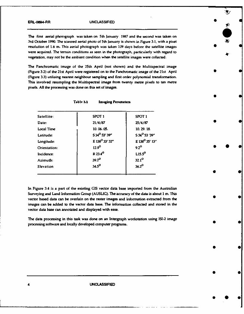
Table 3.1 Imaging Parameters
Satellite: SPOT 1 SPOT 1
Date: 21/4/87 25/4/87 0
Local Time 10.06.05. 10. 29. 18.
Latitude: S 340 53'39V S 340 53'39"
Longitude: E 1380 33' 32" E 1380 35' 13"
Orientation: 12.90 9.20 * * *Incidence: R 23.40 L15.50
Azimuth: 39.20 32.10
Elevation 34.50 36.20
In Figure 3.4 is a part of the existing GIS vector data base imported from the AustralianSurveying and Land Information Group (AUSLIG). The accuracy of the data is about 1 m. Thisvector based data can be overlain on the raster images and information extracted from theimages can be added to the vector data base. The information collected and stored in thevector data base can annotated and displayed with ease.
The data processing in this task was done on an Intergraph workstation using ISI-2 imageprocessing software and locally developed computer programs.
4 UNCLASSIFIED

UNCLASSIFIED ERL-0694-RR 0
44,
0
* S
Figure 3.1 Scanned colour aerial photograph of the study areataken on 5 Jan 1987.
UNCLASSIFIED5

UNCLASSIFIED ERL-0694-RR •
0S
S
* 0
* 0
Figure 3.2 Multispectral SPOT image of the areataken on 21 April 1987. Pixel resolution 20 m
UNCLASSIFIED 7

UNCLASSIFIED ERL-0694-RR
0!
* .
0I
* S
Figure 3.3 Pancromatic SPOT image of the areataken on 21 April 1987. Pixel resolution 10 m
UNCLASSIFIED 9
0 0 0

UNCLASSIFIED ERL-0694-RR S
0
0
*" .
0!
0i
S buildings1- fencesj-- runways/apron/txia- sealed roads aia- unsealed roadsJ
Figure 3.4 Digital map of the area (source AUSLIG). Resolution im approximate.
U A F
* 0!
UNCLASSFIED _
* 0 0

UNCLASSIFIED ERL-0694-RR
4 PATTERN RECOGNITION 0 0
The term pattern recognition is used to mean various aspects in image processing literature.Pattern recognition is a classification problem, including clustering and supervisedclassification (Young and Calvert, 1974). Prior to classification, however, a detection stage 0may be involved depending on the technique used. Sometimes the term 'pattern recognition' isstretched to include image enhancement. Some authors constrain it to mean 'imageunderstanding' that is mainly concerned with representing real world objects and managingthem in a computational environment (Sleigh,1983). Feature extraction is another termfrequently used to mean pattern recognition. However, the use of the term 'feature extraction'will be avoided in this report as the term 'feature' is some times used to mean the bands in theimage and feature extraction in such a context refers to the selection of features (bands) or thereduction of the dimensionality of the data set without significantly losing the information
content. In this report, 'Pattern recognition' is used to mean the classification of the images toobjects of known physical description.
4.1 Pattern recognition - a brief review
There are three main approaches to pattern recognition:(a) statistical pattern recognition,(b) optical and digital pattern correlation (template matching), and(c) model-based vision. A good review of these techniques is available in Mundy (1991).
Statistical pattern recognition can be implemented using Bayesian classifiers, clusteringprocedures or more recently neural-net classifiers. The strength of statistical patternrecognition lies in its ability to process multi-dimensional data in a multi-dimensional spacewithout knowing the spatial structure of the data. However, with some difficulty thespatial structure of the data may be incorporated in the statistical procedures for a betterresult. Other techniques described below process variates of the multivariate data
separately.
In the technique of pattern correlation, an instance of the object is taken as a template and itscorrelation with different parts of the input image is determined. The targets are determinedbased on maximum correlation achieved. Correlation techniques can be made translation,rotation and scale invariant. However, correlation is not intensity invariant. Variation inshadows can give false results (Mundy,1991).
In model based pattern recognition procedures the image is initially processed to extract a 2Ddescription of the objects. Then, using a 3D model, a 2D representation is predicted. Theclassification is achieved based on the prediction accuracy. The advantage of this techniqueis that it is intensity invariant. However, the technique suffers as the pixel resolutionbecomes coarser. This limits its application in pattern recognition in civilian satellite images.
UNCLASSIFIED 13
ERL-0694-RR UNCLASSIFIED
From the above discussion it is clear why the statistical pattern recognition is still the )favoured approach in remote sensing applications. 0
4.2 Statistical pattern recognition - which technique to use ?
In the image classification context two terms are commonly encountered: feature class andinformation class. Feature classes refer to data clusters having similar statistical propertiesand they may or may not have any bearing on objects that we recognise. On the other handinformation classes refer to classes of objects that we identify as types of land cover.
The discrimination processes used for extracting feature classes are commonly called'clustering'. Clustering is mainly used for studying the data structures in terms of separablegroups of data points. As this process requires no supervision whilst training the process to 0
identify objects it is called 'unsupervised classification'. This process is not generally used inremote sensing investigations as the clusters are hard to relate to the terrain objects that theuser intends to investigate.
Information classes are extracted from the images by training a statistical process to recognise 0
objects from their spectral properties. The processes are trained to discriminate betweeninformation classes by providing a sufficiently large number of samples, usually more than100, of each information class. As the user supervises the process during training, thetechnique is called 'supervised classification'. In this report only supervised classificationtechniques are used. 0 O
4.3 Digital Pattern recognition versus aerial photo-interpretation
Digital classification of satellite images can produce a greater variation within informationclasses than visual interpretation of aerial photographs or ground truthing can produce, 0particularly regions of uniform texture (Sali and Wolfson, 1991, Hyland et al, 1988). Thisissue is explained in Klemas et al (1975) with examples. The finer resolving power of theclassifiers can often be disadvantageous as it causes graininess or 'salt and pepper effect' inclassification results.
To overcome the graininess of the classification a post-classification, line preservingsmoothing filter was passed over many of the classified images in this report. The filter is apart of the ISI-2 image processing software. The effect of this is to remove any single orisolated small groups of pixels that represent the finer classification not perceived by thehuman eye. It does however preserve groups of pixels of a prescribed length or greater that 0could represent linear features in the classified image. All GMLC classified results shown inthis report are post-processed.
4.4 Robustness of common classifiers
* 0In developing classification procedures one may encounter following three possibilities(Lachenbruch and Goldstein,1979):
I. the probability distribution of data is completely known,
0 0
14 UNCLASSIFIED
* 0 0
UNCLASSIFIED ERL-0694-RR
2. the probability distribution of data is known or assumed but the parameters are
3. nothing whatever is known and a distribution is not assumed •4r
In remote sensing applications the first case is very rare. If the distribution is completelyknown the posterior probability may be easily computed and the pixel can be assigned to theclass with the highest probability. The second case is very common and usually amultivariate normal distribution is assumed. The unknown parameters are obtained from the -maximum likelihood estimates of training areas. Class membership is assigned according tothe maximum likelihood rule.
In the second case, nothing is assumed about the underlying multivariate distribution and theprocedures are called non-parametric; that is, they are distribution free. In principle non- 0 0
parametric procedures should provide better results if the samples are large, as in remotesensing applications, and when the distributions are not normal (Lachenbruch andGoldstein,1979).
Two classifiers are well known in classification or discriminant analysis literature: Fisher's 0 0linear discriminant classifier (LDC) and Gaussian maximum likelihood classifier (GMLC).Both of these techniques provide optimal results when the data have a Gaussian or Normaldistribution.
GMLC is by far the most widely used classifier in remote sensing studies. By definition, the 0 0
classifier assumes multivariate normal distribution for data points. Although thisassumption is violated by most of the data set we encounter, the technique works very well.The technique is fairly robust to violation of Gaussian model (Richards,1986).
LDC is not commonly used in remote sensing investigations. However it has certain qualities, 0apart from the simplicity of its implementation, which merit brief consideration here.Shettigara (1991a) has compared the performance of LDC and GMLC. His study showed thatLDC is more robust than GMLC. LDC is widely and quite erroneously associated withmultivariate distribution. It is true that LDC gives optimal results for multivariate normaldata. However, it is not restricted to any particular distribution. The technique maximises • 0distance, in spectral data space, between class means (Anderson,1982). LDC is a legitimate
non-parametric technique.
Another family of non-parametric techniques that have become popular recently is based onArtificial Neural Networks (ANNs). A particuldr kind of ANN, the multi-layer perceptron(MLP) can be used for supervised classification. The MLP does not use any data distributionmodel and in principle should be able to fit the best possible decision surface between twoclasses, giving 100% accuracy for separable classes. In practice such accuracy is not achievedfor a variety of reasons; e.g. training is a long process and is often curtailed. Some researchersclaim that ANNs perform better if they are trained on properly pre-processed data sets(lisaka and Russell,1991). However, most cases documented in the literature do not share thisview. In general, accuracy has been found to be comparable with standard GMLC techniques(Benediktsson and Swain, 1990; Hepner et al., 1990; Sheldon, 1990; Kanellopoulous et al.,
U 0
UNCLASSIFIED 15
* 0

ERL-0694-RR UNCLASSIFIED 0
1991; Heermann and Khazenie, 1992). The results of using ANNs for classification are
presented later in the section.
4.5 Choice of classes and training areas
To classify an image using supervised classification, areas need to be selected that are
representative of classes chosen. These areas, known as training areas, are the key to a
successful classification. When selecting training areas for supervised classification three 0
important factors should be considered (loka and Koda,1986). The training areas should
(a) fully reflect categorised theme information which is visually interpreted and
recognised,(b) contain all possible multispectral features inherent in each category, and(c) satisfy the a priori statistical assumptions/conditions of the classification
procedures.
As stated, training data have to represent as much spectral variation within the class as
possible. This is particularly highlighted by Wright and Harris (1988). They found that the 0
accuracy of classification improved when more than one training area represented a class. In
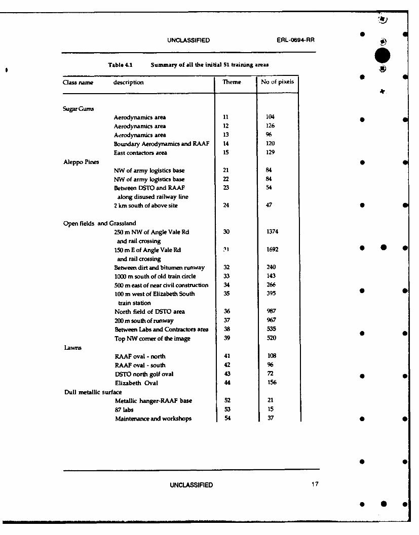
this study, initially 51 known training areas were chosen using the knowledge gained from
analysing aerial photographs and extensive ground truthing of the study area. All the 51
training areas are identified in a theme file by giving a unique number to pixels in eachtraining area (Table 4.1). All the training areas represent a recognisable land cover (class)
and care was taken not to overlap boundaries into other classes.
The 51 training areas were then reduced to 11 super-training areas (classes) initially, by
merging training sets as shown in Table 4.1. Later, one of the classes, dull metal, was further
divided into two classes, namely dull metal and specular metal. The reason for this will be 0
explained later in this section. The merging of training areas was necessary because many
training areas represented a single meaningful physical class.
To decide how to merge smaller training sets into super-training sets, graphical and
statistical techniques were used apart from considering the physical appearance. The S
multispectral data for each training area were plotted as scattergrams and their distributions
relative to other classes were used as a guide to pool some of the training areas. The Jeffries-
Matusita (J-M) distance measure was also used as a guide to merge different training areas.J-M distance is a statistical measure for determining the separability of 2 classes. As the
separability increases, the J-M distance asymptotically approaches a value of 2.0. The
distance measure has the advantage of varying the measure scale by stretching the smaller
class separations and contracting larger class separations.
16 UNCLASSIFIED
vr.
UNCLASSIFIED ERL-0694-RR
Table 4.1 Summary of all the initial 51 training areas
Class name description Theme No of pixels
Sugar Gums
Aerodynamics area 11 104
Aerodynamics area 12 126
Aerodynamics area 13 96
Boundary Aerodynamics and RAAF 14 120
East contactors area 15 129
Aleppo Pines 0
NW of army logistics base 21 84
NW of army logistics base 22 84
Between DSTO and RAAF 23 54
along disused railway line
2 km south of above site 24 47 •
Open fields and Grassland
250 m NW of Angle Vale Rd 30 1374
and rail crossing
150 m E of Angle Vale Rd 't 1692 * 0and rail crossing
Between dirt and bitumen runway 32 240
1000 m south of old train circle 33 143
500 m east of near civil construction 34 266
100 m west of Elizabeth South 35 395 0 5
train station
North field of DSTO area 36 987
200 m south of runway 37 967
Between Labs and Contractors area 38 535
Top NW corner of the image 39 520 •
Lawns
RAAF oval - north 41 108
RAAF oval - south 42 96
DSTO north golf oval 43 72
Elizabeth Oval 44 156
Dull metallic surface
Metallic hanger-RAAF base 52 21
87 labs 53 15
Maintenance and workshops 54 37
U 1
UNCLASSIFIED 17
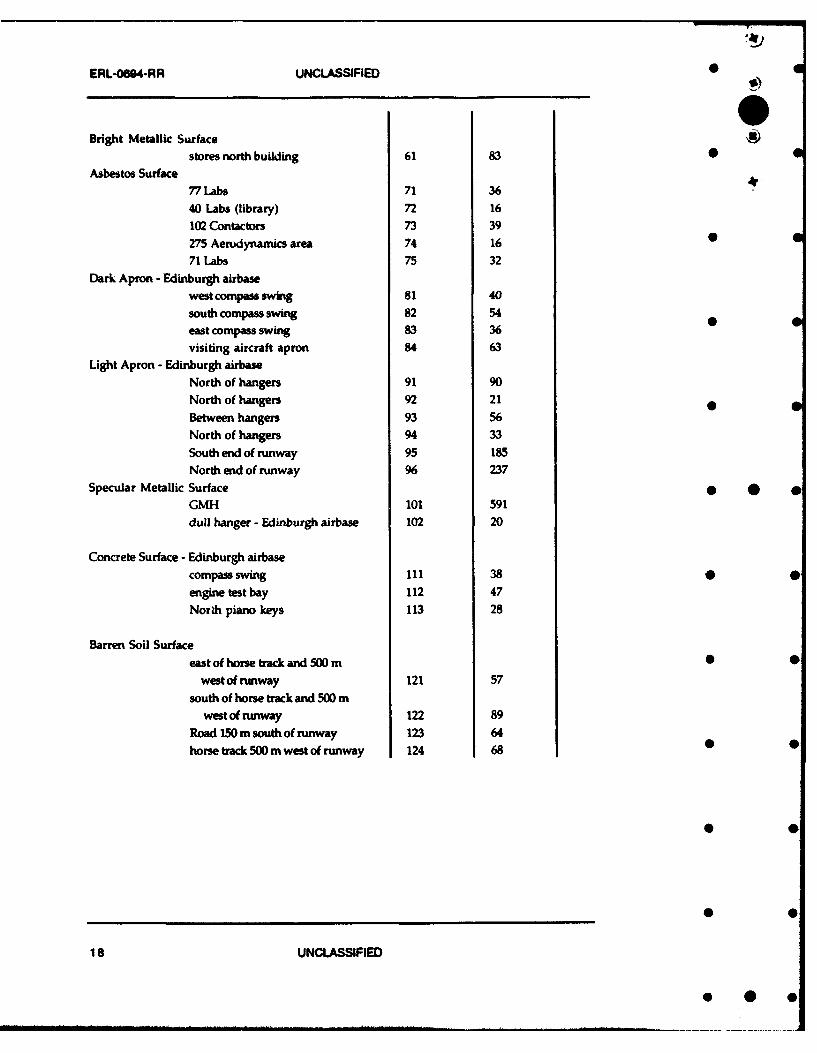
ERL-0604RR UNCLASSIFIED 4
Bright Metallic Surface ')stores north building 61 83 0 •
Asbestos Surface77 Labs 71 3640 Labs (library) 72 16102 Contactors 73 39275 Aerodynamics area 74 1671 Labs 75 32
Dark Apron - Edinburgh airbasewest compass swing 81 40south compass swing 82 54east compass swing 83 36 0visiting aircraft apron 84 63
Light Apron - Edinburgh airbaseNorth of hangers 91 90North of hangers 92 21 0 0Between hangers 93 56North of hangers 94 33
South end of runway 95 185North end of runway 96 237
Specular Metallic Surface 0 * *GMH 101 591dull hanger - Edinburgh airbase 102 20
Concrete Surface - Edinburgh airbasecompass swing 111 38 0engine test bay 112 47North piano keys 113 28
Barren Soil Surfaceeast of horse track and 500 m 0 0
west of runway 121 57south of horse track and 5W0 m
west of runway 122 89Road 150 m south of runway 123 64horse track 500 m west of runway 124 68
18 UNCLASSIFIED

UNCLASSIFIED ERL-0694-RR 0
27S
250
US .
S "•2WI
17S_ _ _ _ _
ISO=1so akpmd pSi • ,,, W OW , guns
1261 ~ pine-
S100. hw"mlam
balm-m WssraS--. -~- bwam so malac
W 76 [ - -7- -- M 1ulc ro d
- -dark btuw~wso-.- concfummftace
2S
greon red Infrarea Osril p.n2
SPOT BANDS
Figure 4.1 Mean spectral responses for 11 super classes with the standard deviations
marked •
4.6 Classifications using Maximum Likelihood
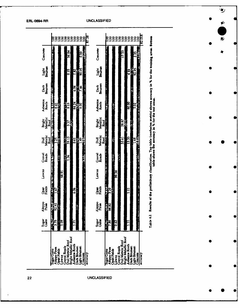
4.6.1 Classification accuracy 0 0The confusion matrix in Table 4.2 shows the initial classification results from using
GMLC. The overall accuracy of the classification in the test areas is 82% that is not
entirely satisfactory. It is felt that an error of about 10% is tolerable, in a subjectivesense. Most errors are in three classes: open fields, dull metallic roof and dark bitumen.
The misclassification is particularly predominant amongst artificial objects. However, 0 0
very few natural objects are misclassified as artificial objects, indicating that thecommonly occurring artificial objects are quite distinguishable from natural objects in
spectral domain.
The misclassification in open fields is due mainly to the inhomogeneity in the class. 0 0This can be seen from the individual training areas within the class, as shown in
Table 4.1. The class might have included, as a part of the open fields, some sparsely
vegetated soil covers which are classified as barren soil covers. As no aerial
* 0
UNCLASSIFIED 19
* 0

ERL-0694-RR UNCLASSIFIED
photographs contemporaneous with the SPOT images are available, it is difficult to
ascertain if the confused areas were low in vegetation.
The confusion matrix reveals few other interesting properties. Amongst artificial
objects most of the misclassification occurs between objects of similar nature For
example, a significant amount o0 pixels in dull metallic roof is classified as bright
metallic roof. Similarly quite a big number of dark bitumen pixels is misclassified as
light bitumen. This misclassification can be generally tolerated as they represent
similar materials and their differenti,,ion may r.ot be necessary for most of theapplications.
4.6.2 Classification blunders •The confusion matrix does not reflect the true cost of classification or mis-classification.
In some cases, although the percentage error in misclassification is small, from the
defence point of view the misclassification can be considered serious. Such errors are
grouped as blunders. Blunder detection should become an important part of any
classifier. 0
For GMLC, there are a couple of misclassifications of serious nature. 12.8% of dark
bitumen pixels are misclassified as bright metallic surfaces. Spectrally these two
classes are quite different as shown in Figure 4.1. The metallic surfaces are highly
reflective in all the bands while the dark apron is highly absorptive in all vands. The * 0 *J-M distance between the classes is 1.99, which indicates that the two classes are quite
separable. This suggests that the misclassification is not due to the overlapping of
classes. A closer examination of the dark bitumen test area revea!ed that there were
aircraft parked on the bitumen that were barely visible in the original multispectral
image. The features in the test area are in fact stationary aircraft on the bitumen. 0 0
Aircraft are metallic and so show a similar spectral response to the metallic class. As
such, the pixels have been correctly classified as metallic surface on the dark bitumen
surface. This demonstrates the capability of a simple classifier to detect small objectsof distinct spectral signature in relation to their background. The object may not be
visible due to their small size in relation to the pixel size and/or due to mixing of two or 0 0
more signatures.
Another serious misclassification has occurred in light bitumen class. 3% for the
bitumen area (Table 4.2), which may be normally considered insignificant, has been
misclassified as asbestos. These errors occur along the boundary between the open field
and light bitumen classes. The reason for this error is suspected to be due to mixing of
open field and light bitumen classes. In Figure 4.2 spectral profiles for light bitumen,
open fields and asbestos surfaces are shown. A profile for the mixed class with equal
parts of open fields and light bitumen classes is presented. As can be seen the spectral 0 0profiles, open fields and light bitumen classes are distinct particularly in the infrared
band. However, when these two spectral classes are combined in various proportions it
is easy to see that the resulting pixel will have a profile similar to that of asbestos
20 UNCLASSIFIED

UNCLASSIFIED ERL-0694-RR 0
surfaces. This illustrates that it is easy to confuse mixed pixels for a totally differentobject
055
50
45
JI
Z 40 /J#
z #
C35 , '
-4s-- open filad30 --- light ttumen
,.,,.-,.. asbestos roof- open field plus lght bittwmen
25'green red infrared pani pan2
SPOT BANDS
Figure 4.2 An illustration of the effect of mixing of two classes - light bitumen surface, •such as runways, and open fields, such as crop an4 pastures.
Another significant misclassification has occurred between dull metallic surface andconcrete surface. A high percentage of dull metallic surface class has been labelled asconcrete surface. From Figure 43 it can be seen that the spread of the concrete surfacetraining areas is relatively small and as such this class splits the dull metallic classinto two distinct classes. This indicated a need for the dull metallic surface theme classto be split into two classes.
UNCLASSIFIED 21
* . 0
ERL-0694-RR UNCLASSIFIED 0
oecooooooeeeo
------ - -- -- -- -- -4000
g• tt
NA
A. A
.3 .0
C-4-
30
C143
-p N
22 UNCLASSIFIED
.•. '0°

UNCLASSIFIED ERL-0694-RR
I-.'1-- -...
iicS..
coa
ra
aid;
a• - • •
S• ..
ral .3 11 30Mfl
UNCLASSIFIED 23
L . . .. . . .......L . ..... .... L..... J,,I•,,, , ,, , .. .. ÷ .. ..-. ...

ERL-0694-RR UNCLASSIFIED 0
20
175 4I
I
>/2 M-- miadc rod1-- -- 4-- dud mdac md
0---- dl mdac rod
7-,- concrele
n= 0, ~~,. 1 p
SPOT___AN_______
750
25
0green red inirared pl Pa2
SPOT BANDS * 0
Figure 4.3 Detailed spectral profile of metallic surface and concrete theme classes
The J-M distance between the dull metallic and concrete classes is only 1.2059. Using therelationship between the J-M distance and the probability of error (Swain andDavis,1978) the maximum error in classifitation is estimated to be of the order of 0
13.6%, given equal prior probability for the two classes. This indicates that the twoclasses are fairly separable. However, the actual error observed is very high. One ofthe possible reasons for this is that the probability distribution function (pdf) assumedfor one or both the classes may be wrong. A look at the scattergrams of the dull metallicclass revealed that it is bimodal, which seriously violates the assumption that data •have normal distribution.
As a result of this finding a further classification was performed, where the dullmetallic class was split into two classes, dull metallic and specular metallic surface.Table 4.3 is the confusion matrix for the new classification. Note that the overallaccuracy of the image classification has improved from 87.38% in the first Sclassification to 90.49% in the second classification if the accuracy test is done on thetraining area. However, if the accuracy is computed on a number of test areas the overall accuracy drops slightly, from 82 % to 81.2%. Bulk of the error is in the open fieldclass. If we consider only the artificial objects the over all accuracy has improved from81.2 % to 87.3 % in the second classification. This level of accuracy is closer to the target •accuracy of 90% set in the beginning of the study. The open field class probably needs tobe further sub-divided into two or more sub-classes in order to improve the over allaccuracy. The new classified image is seen in Figure 4.4
24 UNCLASSIFIED
..... ... ..

UNCLASSIFIED ERL-0694-RR 0
,, 0
.. ' :•v •:•
0
0
0
Maximum Likelihood classification
man-made Accuracy % natural Accuracy %
barren soil surface 98.47 gums 85.78
O dull metallic surface 77.08 O pines 88,82
* specular metallic surface 87.58 CD open fields and grassland 69-28
* bright metallic surface 96.67 3 lawn 99.38
asbestos surface 97.44
* dark bitumen surface 100 •
light bitumen surface 78.52
0) concrete surface 84.78
overall classification accuracy 84.41 %
Figure 4.4 Result of maximum ýketiiho),d classification after sub-dividing dull metalclass. The accuracy figures are with res,:,.ct to test areas. The overall accuracy of artificial
objects is 87.3%
UNCLASSIFIED 25

UNCLASSIFIED ERL-0694-RR •
4.7 Classifications using Multi-Layer Perceptron
4.7.1 Some notes on the application of MLPs to classification 0
The classification power of the multilayer perceptron has been recognised for a numberof decades, but only since the work of Rummeihart et al (1986) has it been possible totrain the MLP from example data. A detailed definition of the MLP and a descriptionof the method of training for this application is given by Whitbread (1992). Since the •application of MLPs to classification of remotely sensed data is relatively newtechnology, some comments on its limitations and difficulties of implementation areincluded here.
The MLP is attractive as a classifier because it is essentially model free, and during
training learns not only the parameters of a class but also the data's probabilitydistributions. In situations where there are naturally occurring non-normal distributions(which challenge GMLC) it is possible to produce an optimal classifier. A particularcase of non-normally distributed data is auxiliary data such as digital elevation data, •which could improve classification accuracy when combined with remotely senseddata. The MLP is also of interest because of the potential to realise it in hardware as afast parallel classifier. However, results presented in this report are based solely on
simulation.
The MLP has not been embraced by the bulk of users of classification processes because ofsome limitations in implementation. Firstly, the MLP is slow to learn; whereas theGMLC measures its required parameters by a single inspection of the training data, anMLP learns its parameters by continued re-inspection of the training examples.Commonly 20,000 inspections can be required to achieve 1% accuracy, and currently most 0MLP classification is done by simulation that multiplies overheads. The secondproblem is that there is no current theoretically based method for choosing the size ofthe MLP necessary for a particular classification task, but it is clear that size isimportant. The current approach is to choose the size using heuristics combined withtrial and error. Heuristics for choosing the MLP size for the task of classifying 0remotely sensed data were developed by Whitbread (1992). The third problem isreliability. Internally, the MLP is a non-linear system, which makes it hard to predictits behaviour as data quality becomes pcor. In model based systems (such as GMLC) weexpect "graceful degradation" of behaviour.
Despite these limitations, the MLP promises potentially better classification accuracythan conventional classifiers, and as well promises greater ease of use, since it is notnecessary to choose training sets that satisfy the a priori statistical assumptions of theconventional procedures (see paragraph 4.5 (c) above). *
UNCLASSIFIED 27

ERL-0894-RR UNCLASSIFIED 0
0
li
0 0
p oU
28 UNCLASSIFIED
- o

UNCLASSIFIED ERL-0694-RR a
i" . • iw ... 64.•
*0*.i94
4 •'l •jr
Neural Network classification 0
man-made Accuracy % natural Accuracy O/
(• barren soil surface 98.47 gums 73.33
•!dull metallic surface 50.00 pines 93.42 0
O specular metallic surface 97.39 C) open fields and grassland 64.84
O bright metallic surface 90.00 •llawn 99.38OD asbestos surface 83.33
dark bitumen surface 75.23 0
•)light bitumen surface 74.16
0) concrete surface 52.17
overall classification accuracy 78.68 % 9
Figure 4.5 Results of ANN classification using classes selected for GMLC classifier.
UNCLASSIFIED 29

UNCLASSIFIED ERL-0694-RR
4.7.2 Classification Accuracy 0
The purpose of the results presented here is to show the utility of the MLP
classification method. 11w results are based on the same training areas as the resultsfrom GMLC presented above and they do not take advantage of the possibility of
relaxing the requirement paragraph 4.5(c) in the choice of training areas.
The MLP used for classifying the multispectral data had three (active) layers
comprising 50, 6 and 12 nodes in the first, second and third layers respectively. TheMLP was trained by adjusting its internal weights using the back propagation procedureof Rumelhart, et al. (1986). (The learning rate was 0.01 and momentum 0.0.) Training
was limited to 20,000 iterations, representing approximately 1600 presentations of 0examples per class. Samples are selected at random for each training iteration.
Table 4.5 Comparison of percentage of comect dassifications by MLP and GMLC.
Theme MLP GMLC
Sugar Guns 73.33 85.78
Aleppo Pines 93.42 88.82
Open Fields 64.84 69.28 * •
Lawns 99.38 99.38
Dirt Roeds 98.47 98.47
Dull Metallic Roof 50.00 77.08
Specular Metallic roof 97.39 87.58
Bright Metallic Roof 90.00 96.67
Asbestos Roof 83.33 97.44
Dark Bitumen 75.23 100.00
Light Bitumen 74.16 78.52 0
Concrete 52.17 84.78
AVERAGE 79.31 88.65
Table 4.4 shows the confusion matrix for MLP classification using the same training
areas as previous experiments and. Table 4.5 shows the relative accuracy of MLP and
GMLC using the same training areas. The MLP has not been able to better the accuracy 0of GMLC in this test. Confusion is of the same kind as GMLC with Gums being
misclassified as Pines, barren soil classified as open field and light bitumen being
classified as dark bitumen. Other more troubling confusions occur between concrete and
metallic reflectors. This is caused mostly by a very strong reflection from these
UNCLASSIFIED 31
* . o0
ERL-O64-RR UNCLASSIFIED a
surfaces. Asbestos is also a problem, with some open fields being confused withAsbestos moves. A major contributor to the good average performance in the GMLC caseis the 100% accuracy for dark bitumen, for which the MLP only gets 75% correct. •
Because the MLP can handle an arbitrary number of inputs, it is possible to reconfigureit to use texture in the training areas. In this demonstration of classification that wasimpractical because the training areas were selected for GMLC and as such were chosen
not to have texture where possible, and many training areas were too small to make anestimate of texture. The potential for the use of the MLP in this way is discussedfurther in the reference by Whitbread (1992).
4.8 Conclusions
This section has described a number of pattern recognition aids for interpreting satelliteimages and has shown how classification can be used to extract man-made objects. Thestandard GMLC has performed better than MLP in this study.
3 0U* S
* 0
32 UNCLASSIFIED
UNCLASSIFIED ERL-0694-RR 0
05 OBJECT HEIGHT DETERMINATION 0
4,
In the last two decades enormous gains have been made in processing satellite images.However, the analyses of the images have remained mostly qualitative in nature, comparedto the field of photogrammetry. This chapter presents an application of remote sensing for •height determination using SPOT images.
Photogrammetrists have been able to extract the heights of objects from aerial photographsusing parallax in stereo-pair photographs. The lengths of the shadows cast by the objects arealso used to determine the heights. If the sun and sensor geometry is known it is fairly simple Sto establish a relationship between the shadow width and the height of the objects. Theabove usages, however, are confined to high resolution photographs or images.
5.1 Shadow - an important part of images
Shadows form a unique part of any image. They are easily detectable as they show a lowintensity in all the multispectral bands. Shadows play a dominant role in image statisticswhich affect image enhancement and pattern recognition. Shadows contain 3-D informationof objects and they have been used in object identification, terrain classification andgeological mapping (Curran,1985). * *Detection of objects by their shadow structures has been performed by many workers in thephotogrammetric community (Venkateswar and Chellappa,1990; Irvin and McKeown,1989;Huertas and Nevatia,1988). All have utilised the nature of shadows around buildings tointerpret the structure of the building. An edge detection routine has been used by Huertas and 0Nevatia (1988) that looks for different types of shadows that represent the corners ofbuildings in the aerial photographs. One of the problems Huertas and Nevatia (1988)encountered in their study was in identifying the shadows. Their technique failed to identifysome areas of shadow or included areas that were not in fact shadow. Venkateswar andChellappa(1990) have used knowledge based procedures to overcome some of these problems. 0 0
Although photogrammetrists have successfully used shadows in aerial photographs forheight determination and object identification, the use of satellite images for similarpurposes is not seen in the literature. The main reason is that the resolution of the civiliansatellite images is much coarser than the aerial photographs and the shadows are not fully 0
defined for short and commonly occurring objects.
5.2 Sun - satellite geometry and the equations
Figure 5.1 shows the sun-satellite geometry as an end view (2-D display of 3-D geometry for 0 0simplicity) for the two SPOT images used in this study. As illustrated in the figure theshadow part seen by the sensor is different for the two images. The width of the shadow,measured along the normal to the object, depends on the azimuths of the sun, image scan lineand the object. The objects are rows of trees in this study (Figure 5.2).
UNCLASSIFIED 33

ERL-0694-RR UNCLASSIFIED 0
In principle the procedure that is presented in this section is suitable for any object that castsdetectable shadows of sufficient length. In the study area rows of trees cast shadows that 0could be used. Buildings were either not tall enough or long enough to cast a consistent shadow.For this reason the shadow detection and height analysis were initially performed on rows oftrees. After establishing the relationship between the shadow widths and the measuredheights, the heights of the unknown objects (buildings) were determined.
For relating sha i --v width to the object (tree) height a few basic assumptions were made. 0 •
Firstly, the object is assumed to be vertical, that is the object is perpendicular to the earth'ssurface. Secondly, the shadows are assumed to be cast from the top of the object and that thetop of the object is also the last part of the object seen from the sensor before the shadowbegins. This assumption is not entirely satisfactory because there could be parts of object,between the illuminated part of the object and the ground shadow, not illuminated by the sunbut seen by the sensor due to the scattered light. The computation assumes that the parts ofthe object not directly illuminated by the sun as part of the shadow. Thirdly, it is alsoassumed that the shadow starts from the tree-trunk line on the ground. Fourthly, as shown inFigure 5.1, it is assumed that if the sensor and the sun are on opposite sides of the object, thenthe sensor is able to see the entire shadow. Lastly, the surface that the shadow falls on is
Image 2 SPOT 1 SPOT 1 Image 1 * * *
band3: panchromatic 25-4-87 21-4-87 bandi: mutispectral-IR
Ssun
actual shadow width 0
ground .as seen by SPOT on 21-4-87
SS.. as seen by SPOT on 25-4-87
shadow tree•
Figure 5.1 End view of the sun-satellite configuration as seen during imaging
34
UNCLASSIRED
* 0 0

UNCLASSIFIED ERL-0694-RR 0
The shadow width along the sun azimuth (Figure 5.1) is given by
ssu = ht/tan(Osu) ............. (5.1)
The shadow width obstructed, along the azimuth of the sensor (Figure 5.1), by the object(tree) in the sensor's field of view
Ssa = ht/tan(Osa) ............. (5.2)
Shadow of the object along the normal to the tree line (Figure 5.2)
Ssun ssucOs(Osun) ............. (5.3)
Shadow obstructed by the object along the normal to the tree line (Figure 5.1) 0
ssan = ssa.COS(Osan) ............. (5.4)
where #sun = #su + 9o- t ............. (5.5)
and Osn = O + 90 -*t ............. (5.6)
The shadow width that is seen by the satellite is given by
s = sson - Sun ............ (5.7) * * *
Note that Ssan = 0 if the satellite is on the opposite side of object from the sun.
N
Osu / sun azimuth
Ssatellite azimuth(scan line)
tree line azimuth
1* 0
I
Figure 5.2 Plan view of the sun-satellite configuration as seen during imaging
UNCLASSIFIED 35
ERL-0694-RR UNCLASSIFIED
For the panchromatic and multispectral image of 21st April 1987 the data are as follows:
Osa = 23.40 and 9su = 55-50
sun = 13.20 and *san =76-50 ............ (5.8)
Using equations (5.1) to (5.4) and (5.8) we get
ht = 0.76s ............ (5.9)
If the tree or shadow line is at an angle to the image scan line, an additional correction needsto be applied to equation 5.9. This is because of the pixelisation of shadow zones. The issue isexplained in Appendix I. The shadow width in equation 5.9 needs to be divided by •Cos(Oscan), where #scan is the angle between the scan lines and the tree line. For the rows of
trees considered #scan = 150. The relation used in this study is:
ht = 0.76 s/cos(scan) = 0.79 s
= ks ............ (5.10)
where k is a constant for objects of fixed azimuth in an image.
5.3 Relationship between shadow width, pixel size and intensities * * *
The above relationships assume that the shadow zones are sharply defined and the pixelsize is infinitesimally small. However, in practice neither the shadow zones are well definednor the pixel sizes are negligibly small in relation to shadow widths. The followingdiscussion presents simple relationship between pixel intensities and shadow boundaries.
If the brightness of the shadow (object) is 10 and that of the background is lb, then thebrightness of a pixel may be approximated to:
If = f 0 + (-Olb ............ (5.11)
where p is the area fraction of shadow in the pixel.
If 10 and lb are known from pure shadow and background pixels, then
f = (If - Ib)/(IO-Ib) ............ (5.12)
There will normally be a threshold fmin such that if f>fm;,i then the pixel is classed asshadow. If not it is classed as background. Clearly, the representation of shudow in the imagedepends on the threshold chosen.
5.3.1 The role of pixel dimension
As we are considering the shadows cast by linear objects of length much greater thanthat of the pixel dimension, we will not lose any generality if we consider the
36 UNCLASSIFIED
* . •

v.
UNCLASSIFIED ERL-0694-RR
relationships only along a profile, say X axis, orthogonal to the object. If the shadow of
length s of uniform intensity is centred at the origin of the profile and the pixel size p is
smaller than the shadow size the intensity of pixels along the profile for various x is
given by
o for xsý p (pixel outside object)2
(x+(s+p)/2) for -(s+p) <x- (pixel partially on theobject)P 2 2
f=' I for"(sP) <_ (pixel wholly within theobject)2 2
(-x+(s+p)/2) for( 2)<x !2 (pixelpartially an theobject)p 2 2
o for x2ýsL) (pixeloutsideobject)2
(5.13)
If the threshold is fmin then the estimated width w of the shadow of width s will be
w(p,fmin) = s+p(1-2pfmin) ............ (5.14)
or in terms of estimated tree heights hest and actual tree heights ht, using * •
relation equation 5.10
hest = ht + kp(1-2fmin) ............ (5.15)
which is a linear relationship between hest and ht with an intercept
kp(1-2fmin) and a slope 1. If fmin is very small, the intercept is roughly kp and if fmin
is very high (near one), the intercept is roughly -kp. The intercept is zero for fmin = 1/2,
which means that the boundary between the shadow and the background is half way
between their respective intensities. In that case the estimated height is equal to the
actual height. This relation assumes that p<s, object and background intensities are •
uniform, and that the measurement errors are normally distributed. In actual practice
the latter two assumptions may not be true. As such, the above equations may only be
used as a guide to arrive at an optimal fmin, through experiments, such that the
intercept and the slope of the regression line in equation 5.15 are close one and zero
respectively. 0
5.4 Shadow Segmentation
5.4.1 Choosing the threshold for delineating shadow zones
In high resolution images one might find a separate peak in the histogram
corresponding to shadow areas, as described by Otsu (1979). In such cases it is easy to
separate the shadow zones. In lower resolution images it is not common to find a
separate peak for the shadow areas. The current study required a general procedure for
UNCLASSIFIED 37

ERL-0694-RR UNCLASSIFIED a
delineating shadows falling on various types of backgrounds. The backgrounds includedlush grass, barren soil, white concrete and black asphalt covers. Experiments were
conducted by choosing various thresholds by varying a in the equation
fmin = - Qo ............ (5.16)
where ga and a are mean and standard deviation of the image. Note that as a increases
the threshold decreases. The weight ct was varied from 1.6 to 0.8 in steps of 0.1. These
two limits were found adequate as at a threshold of 1.6a most of the shadow areas were
mis-classified as non-shadow areas and when a threshold of 0.8 a is used mobt of the
non-shadow areas were classified as shadow areas.
5.4.2 Measurement of shadow width 0
From the accuracy point of view it would be better if the shadow width could be
determined from SPOT panchromatic bands which have a resolution of 10 m. However,
in panchromatic bands both the trees and shadows appear equally dark and the
separation of the trees and shadows is not possible. However, in the infrared band of
the multispectral image (Figure 5.3), which has a resolution of 20 m., the trees show a
significantly higher reflectance than the surroundings and the shadow zones. In
principle only the infrared band would suffice to determine the shadow width, butwith a lesser precision due to its coarser resolution. In order to improve the accuracy of * * *the estimate of the shadow width it was decided to use the panchromatic and infrared
bands together. Another reason for using the combination is for shadow detection
accuracy. A low value in infrared band does not necessarily mean that it is a shadow
zone. For example bitumen surface gives a low reading in infrared, but a relatively
higher value in panchromatic images. A combination of panchromatic and infrared 0
bands would detect shadow zones better.
The image data consisted of an infrared band of a SPOT multispectral image and two
panchromatic bands taken on two different days, as shown in Figure 5.1. The three
bands were co-registered to form a 3-band image using control points at the ground level. 0
Initially, for a chosen threshold, fmin, shadow areas that were common to all the three
bands were delineated. Using the same fnmn shadow areas common to only the infrared
band and the panchromatic band of image 1 (Figure 5.1) were determined. No
significant difference was found between the shadow zones determined in the two
experiments. For this reason only the two bands of image I (Figure 5.1) were used for
further investigation.
Figure 5.4 shows an example of the shadow segments delineated from the images. Using
the segmented shadow areas an average shadow width is measured for each row of
trees. As can be seen from Figure 5A, the edges of the shadow areas are not straight.
This is because of the alignment of the rows of trees at an angle to the scan lines andalso due to the coarse pixel resolution. Due to the jagged nature of the shadow
boundaries the estimation of the width is complicated. The average width was
38 UNCLASSIFIED
* .. . . .. . .

UNCLASSIFIED ERL-0694-RR S
estimated by measuring the area covered by each shadow zone and then dividing it bythe length of the zone.
In order to accomplish the above procedures the shadow zones were vectorised using the
program RASVECO available on the Intergraph workstation. The areas bound by the
polygons corresponding to the shadow areas were calculated using the MicroStation
CAD software. Shadows of length less than 50 m were neglected. From the shadowwidth estimates of the tree heights were computed using equation 5.10.
U 3
@ 0
UNCLASSIRiED 39

ERL-0694-RR UNCLASSIFIED 0
* 0
* 0l
40 UNCLASSIFRED
S. . . . . . . . . . . . __ . . . . . . . . .. . . . .. . . . .. .• i . .. . r l l I ~ • . . .. . . . . • l i i • i i i I . . . . .. . . . il*.. . . .. i . . . . .0_
A1ILUNCLASSIFIED ERL-0694-RR
0 t
* S:
*
Figure 5.3 Infrared SPOT image of the study area. The rows of trees used in the study are
marked and the buildings whose heights are estimated using the tree shadows are shown at -
the lower right hand corner.
U 4
UNCLASSIFIED 41

UNCLASSIFIED ERL-0694-RR
5.5 Result and discussion
Most of the shadow zones shown in Figure 5.4 are correctly identifiable as cast by the rows of 0
trees. However, false identification of shadow areas has also occurred. The dark bitumen at
the west of the image and some wet market garden areas in the south western part of the
image (Figure 5.3) were mis-classified as shadows. In this study no automatic procedureshave been developed to isolate 'false shadow' zones.
a row of C;
linear shadow zones
=:Zap
Figure 5.4 Shadow zones, shown as polygons, delineated using the thresholding
procedure on the infrared and the panchromatic bands
There are some rows of trees that are parallel to the principal plane of the sun or the sunazimuth which do not cast shadow. No height estimation could be made for rows of trees
with such an orientation.
Eight sites were selected for tree height estimation. At these eight sites tree heights were
also measured. Table 5.1 summarises the measured tree heights and the estimated heightsfrom the shadows.
UNCLASSIFIED 43
/

ERL-XI04-RR UNCLASSIFIED j
Table 5.1 Estimated and actual tree heights
site Shadow length m Estimated tree Measured average Standard deviationheight m tree height m of measuremnt m
2 29.720 21.82 17.90 1.41
1 27.635 20.28 17.45 2.34
3 35.390 25.98 15.00 1.37
4 29.705 21.81 17.% 1.35
5 25.191 18.50 15.82 1.11
7 11.119 8.25 11.76 0.64 0
6 28323 20.80 16.14 1.26
8 25.359 21.55 17.11 0.63
Figures 5.5 shows the regression lines of estimated heights computed from shadow widthsdetermined by using different thresholds and actual tree heights are shown. For the sake ofclarity, regression lines and data points for only a few thresholds are plotted.
Notice that the correlation between the obserncd heights and the estimated heightsdeteriorate drastically when the threshold is increased from 1.2o to 1.1c. The variation ofheight estimates are shown for all the sites with these two thresholds. The height estimatesincrease systematically, as expected, for all the sites except site 5. The increase in heightestimate for site 5 is dis-proportionately high. This is due to the inclusion of non-shadowareas in the shadow estimates. Notice that the regression line for any of the cases involving 0thresholds up to 1.L1 do not pass through the origin as ideally we would have liked to. Toachieve an intercept of zero the threshold has to be varied between 0.9a and 0.8a. However,as we increase the threshold above 1.2a background areas are increasingly classed as shadowareas. Thus the increase of threshold beyond 1.2a is not justifiable.
The coefficient of determination (r2 ) for thresholds higher than 1.2a is high (Figure 5.5).This indicates that the shadow estimates are very well correlated (correlation coefficient of0.832 for threshold 1.2a) to the measured tree heights. One point worth considering is thatwhether the number of points used for the regression is large enough. The probability ofgetting a correlation of above 0.8 is less than 6% when the two variables are uncorrelated, and 01
the number of measurements involved is more that 6 (Taylor, 1982). This suggests the results ofregression are reliable.
* 0
44 UNCLASSIFIED
. .. 0
• 4lUNCLASSIFIED ERL-0694-RR
0 30
25 5t
/ I.
h'I
/ '/'o S ,
r• ,4,E•/
/ .
"30 6. Standard deviations
M 20 - y= 1.579x +3.274 r2 =O0.876
* 1.1 Standard Deviationsa2IS "
S1 "y1752.6 r" O.•30
0 1.2 Standard Deviations
"- --- y =1.598x - 6.029 r2 = 0.692
1' ," • 1.5 Standard Deviations
",' -... y = 1.754x- 11.524 r 2 =0.829
0 5 16 15 20 2S 30 35 40
ACTUAL AVERAGE KEIGIITS OF TREE ROWS
Figure 5.5 Regression lines for different thresholds. Notice that the estimatedheights vary systematically for all the sites except for site 5. Th drastic variation
for site 5Sis attributed to the inclusion of background areas when the threshold isincreased from 1.2 to 1.1c.
* @1
Figure 5.6 shows how estimated heights vary with various thresholds. Each line in the plotcorresponds to a row of trees and a location. The plot reveals that all the estimates varysharply between 1.2a and 1.1a, indicating that non-shadow areas are getting incorporated inthe shadow estimates. This point is vividly illustrated by the site 5 estimate. As explainedabove the estimate for site 5 jumps drastically between 1.2 and 1.1a. This indicates that the 0optimum threshold for separating shadows from the background exists between 1.2a to 1.1o.
It is also interesting to note that as the threshold is increased or decreased from 1.2a theheight estimates tend to be asymptotic. As such, the estimates for rows of trees within a rangeof heights tend to converge to a common value. These properties are currently being 0investigated using theoretical models. However, some heuristic explanation for this propertymay be given here.
UNCLASSIFIED 45
(
S.. . . . . . . . . . .. . .. ... . . . .. . . ll i d . .. . . . . .• . . .. . . . ." i . . . . ... .. .•.. ... . . . . .. 0 - 0 ]lnt i ,

ERL-0694-RR UNCLASSIFIED 0
In Figure 5.7 intensity curves are sketched for shadow zones of sharp boundaries and varyingwidths. The curves mimic the smoothing of sharp boundaries due to the point spread functionsof the sensors. As can be seen, at A and B the intensity curves tend to overlap and at 0 theyshow maximum separation. Considering the noise inherent in images it may be expected thatthe closely spaced intensity curves can be inseparable at thresholds A and B. This explainsthe convergence of estimated tree heights at two extreme thresholds.
40 0
3 5- •ACTUAL TREEHEIGHTS SITE
30 0 11.757 7
20 15.817 5
-i-"O" 15.928 6
S20-181 17.507 1
5 ------ 17.717 8 0
10 0 17.895 2
5- --- ,&-- 18.015 4
0.8 0.9 1.0 1.1 1.2 1.3 1.4 1.5 1.6
THRESHOLD (STANDARD DEVIATION)
Figure 5.6 Variation of estimated tree height with threshold. Notice that the 0estimated heights converge at two extreme thresholds. Also the gradient variation is
maximum between 1.2 and 1.la
Figure 5.8 is a three dimensional (3-D) display of the tree heights interpreted from theshadows in the image. The heights of the rows of trees has been vertically exaggerated by a 0factor of two. The 3-D display provides additional information apart from highlighting thetree heights. The gaps between the rows of trees get exaggerated, which otherwise may go un-noticed. For example, the rows of trees on the extreme left hand side of the image show a gapwhich is not evident in the 2-D display in Figure 3.2. The other rows of trees also give theimpression of having numerous gaps. However, those could be artefacts created by the 0 0pixelisation of shadows.
46 UNCLASSIFIED

UNCLASSIFIED ERL-0694-RR
Background 123I0I
00
29I.-
BShadow
Figure 5.7 A sketch of intensity variation across shadow boundaries to demonstrate the 0
variation of separability at various thresholds. The vertical lines 1, 2 and 3 represent
the three sharp boundaries between shadow and background. The three curved lines
represent the intensity variation as seen by the sensor across the three boundaries. Thelines A, B and 0 represent the three thresholds and their thickness represents the
possible noise level. At thresholds A and B the separation of the three curved lines is •
difficult to achieve, particularly considering the noise. At threshold 0 the curves
stand separated.
* 0
Figure 5.8 A three dimensional display of some rows of trees in the DSTO area.
U 47
UNCLASSIFIED 47
S.. . . .. . • - - .. ...•, n ". .. . .. .. " , ,, . - , . . . . .. ........ . ......... ...
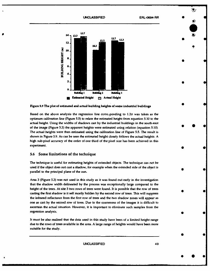
UNCLASSIFIED ERL-0694-RR 0
14 3 13.7
13 17 12.312.
A 10.
6.
2. 0
0Seidg 1 DWýq 2 MAg6 3
* Estinated Height rl Actual Height
Figure 5.9 The plot of estimated and actual building heights of some industrial buildings
Based on the above analysis the regression line corresponding to 1.2o was taken as theoptimum calibration line (Figure 55) to relate the estimated height from equation 5.10 to theactual height. Using the widths of shadows cast by the industrial buildings in the south-east
of the image (Figure 5.3) the apparent heights were estimated using relation (equation 5.10).The actual heights were then estimated using the calibration line of Figure 5.5. The result is
shown in Figure 5.9. As can be seen the estimated height closely follows the actual heights. Ahigh sub-pixel accuracy of the order of one third of the pixel size has been achieved in this
experiment.
5.6 Some limitations of the technique
The technique is useful for estimating heights of extended objects. The technique can not beused if the object does not cast a shadow, for example when the extended side of the object is
parallel to the principal plane of the sun.
Area 3 (Figure 5.3) was not used in this study as it was found out early in the investigation
that the shadow width delineated by the process was exceptionally large compared to theheight of the trees. At site 3 two rows of trees were found. It is possible that the row of trees
casting the first shadow is it self mostly hidden by the second row of trees. This will suppressthe infrared reflectance from the first row of trees and the two shadow zones will appear as
one as cast by the second row of trees. Due to the coarseness of the images it is difficult toascertain the actual situation. However, it is important to eliminate such samples from the
regression analysis.
It must be also realised that the data used in this study have been of a limited height range
due to the rows of trees available in the area. A large range of heights would have been more
suitable for the study.
UNCLASSIFIED 49
.0 * 0
ERL-0UW4-RR UNCLASSIFIED 0 S6 NEW IMAGE ENHANCEMENT TOOLS
Many of the decisions by defence agencies or resource industries are done by visual patternrecognition as opposed to the numerical tchniques explained in section 5. Image enhancemntplays a major role in improving the visual pattern recognition in the images (Woodruff and 0Newsam, 1992). The background discriminant analysis technique described in section 4 is atool in which objects of interest are enhanced in a multispectral image by suppressing thecontribution of background information. In this section 2 other issues in image enhancement areaddressed.
6.1 Smooth image zooming
The commercial satellite images have coarser resolution compared to aerial photographswhich are conventionally used in defence for pattern recognition purposes. While displayingsuch images the objects look blocky making the recognition of the objects difficult. The 0problem becomes more severe as the observer zooms into a small area. While no extrainformation can be created in the blocky image once it is created, one can improve thepresentation of the image to assist the human observer in understanding the image. Imagesmoothing while zooming (Woodruff and Newsam, 1992) is one way to reduce the blocking. Inhis approach, Newsam (1992) used a smooth interpolant to sub-sample an image to higher • 0apparent resolution. An approximation is then determined to the interpolant using FFTs.
Using a similar approach as that of Newsam (1992), in this study cubic convolution is used forinterpolation while zooming. Cubic convolution is a process originally developed for Landsatimage reconstruction. Cubic convolution is simply another interpolation techniqueimplemented by convolving the image samples with a smooth, spatially limited one-parameter functions constructed by joining cubic polynomials in a spline like fashion. It isgenerally accepted that this interpolation process gives a good compromise betweencomplexity of computation and accuracy (Billingsley,1983). The technique is generallysuperior to the standard image restoration procedures and it can be adapted to the frequencycontent of the image (Park and Schowengerdt,1983).
In the field of remote sensing the cubic convolution interpolation is extensively used forresampling. The procedure is generally available in commercial software for registeringimages of two different pixel resolutions. Due to the increased processing speed and the 0 0possibility of subsampling the images in the main memory in near real time exists in mostmachines.
An existing command line procedure in ISI-2 image processing software on an Intergraphworkstation was adopted for smooth zooming. The existing utility 'image to image' in ISI-2can be used to subsample an image using cubic convolution procedure. The input parameters forthe utility include the displayed image name, the name of the output (smooth zoomed) imageto be displayed, and a file containing a table of ground control points. In the normal
50 UNCLASSIFIED
* 0 0
UNCLASSIFIED ERL-0694-RR
application of the utility the ground control points are selected manually by comparing theimage to be resampled and the reference image. In the current work the table of ground controlpoints was generated automatically based on the zoom required. Table 6.1 demonstrates howthe table is generated. The whole sequence of generating the ground control points table andsmooth zooming of the image can be implemented as a command procedure and assigned to afunction key. Depending on the size of the image and the processor speed the display can be innear real time.
Table 6.1 Ground control poins for zooming by a factor X
GCP location Input Image Input Image Zoomed Image Zoomed Image •line pixel line pixel
top left comer 1 1 1 1
top right comer 1 n I n.X 0 •
bottom left m 1 mX 1comer
bottom right m n mX nX * 0corner
Figure 6.1 is for demonstrating how an image may be zoomed in to achieve a magnification of8. Figure 6.1(a) shows a sub-image of the GMH industrial complex adjoining the DSTO area.The image is shown at its full resolution of 10 m. Figure 6.1 (b) is the same image degraded to80 m resolution, which is equivalent to a compression factor of 64. Each pixel in Figure 6.1 (b)is a mean of a 8x8 window. Figure 6.1 (c) is the smooth zoomed image derived fromFigure 6.1(b) using cubic convolution. In Figure 6.1 (d) smooth zooming is achieved by the
procedure of Newsam (1992). As can be seen the reconstructed Figures 6.1 (c) and (d) closelyresemble the original full resolution image of 10 m. resolution in Figure 6.1 (a). • •
At this stage the results of smooth zooming from the two techniques have not been comparedin any quantitative sense. The purpose of this example is simply to demonstrate the use of anexisting remote sensing tool for a fairly complicated mathematical operation. The results
from the two techniques are comparable. 0 0
Figure 6.2 is similar to Figure 6.1. The magnification in this case is 16 which is equivalent to256 fold data compression Clearly, the smooth zooming has not restored the image inFigure 6.2 (b) to the quality of Figure 6.2 (a). The zoomed images in Figures 6.2(c) and (d) alsosuffer form the distracting contouring effect. The contouring effect can be reduced to some 9 0extent, if desired, by dithering (Jain,1989).
From the above two examples it may be recommended that up to 8 times magnification can beachieved using smooth zooming without significantly degrading the image. Near real time
UNCLASSIFIED 51

ERL-0694-RR UNCLASSIFIED 0
smooth zooming, using cubic convolution, can be implemented on most remote sensing imageprocessing systems using vendor provided utilities. A)
4r
(a) (b)
• -
0 .
(c) (d) 0
Figure 6.1 Smooth zooming by a factor of 4.(a) the original image of 10 m resolution(b) degraded image with 40 m resolution(c) image in (b) is smooth zoomed by a factor 4 using cubic convolution, 0 0(d) image in (b) smooth zoomed by a factor 4 using the interpolation
technique of Newsam(1992)
52 UNCLASSIFIED
0 S 0
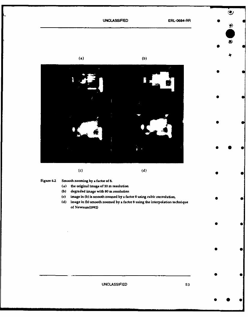
UNCLASSIFIED ERL-O694-RR S
0
00
(a) (b)
i0
(c) (d)
Figure 6.2 Smooth zooming by a factor of 8.(a) the original image of 10 m resolution(b) degraded image with 80 m resolution(c) image in (b) is smooth zoomed by a factor 8 using cubic convolution, *(d) image in (b) smooth zoomed by a factor 8 using the interpolation technique
of Newsam(1992)
UNCLASSIFIED 53
* 0 0

0ERL-0694-RR UNCLASSIFIED
6.2 Multispectral image enhancement by merging higher resolution 0panchromatic data
The availability of high resolution data in the form of panchromatic image data or scannedaerial photograph has given rise to a host of procedures to enhance coarser resolutionmultispectral images. By merging, the advantage of having both spectral and spatial Sresolution is gained. This will enhance the target recognition task. Shettigara (1992) hasshown that the merging process can be achieved in one simple step of linear transformation.Due to this simplification it is possible to achieve merging of data in near real time andenhance the image on the screen at the location of interest.
To demonstrate the power of merging, the multispectral SPOT image of air base (figure 6.3.a)was merged with the panchromatic image taken at the same time (figure 6.3.b). As can beseen, merging has enhanced the parked aircraft on the apron, which is not clearly visible inthe original multispectral image.
0The merging was achieved in 3 steps:
1. the total intensity component of (a) was computed,2. the total intensity component was substituted by the panchromatic data and,3. the higher resolution information content in the new intensity component is re-distributed to the multispectral bands. The resultant image is shown in Figure 63(b). • 0
Data merging can be achieved in many other ways. For more details the reader may refer toShettigara (1992).
• U
54 UNCLASSIFIED

UNCLASSIFIED ERL-0694-RR
pancxornacuw~ge
ofigional SPOT multiuspectml enhanred SPOT miutspectmlimae (20m pixels) iMAge (IOm pixels i pplnt)
iigure 6.3 Merging of panchromatic image with the SPOT multispectral image
(a) multispectral image
(b) enhanced image bv merging panchromatic image(c) Notice the 4 aircraft, below the circular compass swing, near the top right S *
hand corner, enhanced in image (b) above
UNCLASSIFIED 55
.0 •
UNCLASSIFIED ERL-0694-RR 0
7 CONCLUSIONS
0
Some new capabilities of commercial satellite images have been demonstrated in this report. .r)
A particular effort has been made to use the images for quantitative purposes.
* It is shown that heights of extended targets can be determined to sub-pixel accuracy(2 to 3 m in our case) using SPOT multispectral and panchromatic images of 20 and
10 m pixels respectively. The high accuracy is achieved by developing a procedure
for optimal segmentation of the shadows. The same procedure may be extended to
determine other dimensions of the targets, such as the widths of roads or the lengths
of buildings.
* The conventional statistical pattern recognition techniques and neural net
approaches are used for object classification. An accuracy of the order of 87 %
achieved in classifying artificial objects. 0
# New techniques are demonstrated for image resolution enhancement in computer
displays. It is shown that an image whose resolution is degraded by a magnitude of
up to 8 can be smooth zoomed, using cubic convolution resampling, to achieve a looksimilar to the original. Smooth zooming can be of great assistance in target detection.
The report clearly demonstrates the ability of multispectral satellite images in enhancing
and detecting targets of defence significance. Objects such as aircraft can be clearly detected
and different types of buildings can be discriminated. It is also possible to determine heights
or other dimensions of targets, larger than the pixel size, to sub-pixel accuracy. As mentioned 0
in the introduction, the applications of commercial satellite images are very much dependent
on the data analysing expertise. In view of this there is a need to re-assess the capabilities of
civilian satellite images in surveillance and intelligence gathering.
0 0
0 0
0
0 0
UNCLASSIFIED 57
0.. 0

ERL-0W04-RR UNCLASSIFIED •
s0
*0
* •
58 UNCLASSIFIED"
0 0 0l
UNCLASSIFIED ERL-0694-RR 0
BIBUOCRAPHY •
Avery T. E., 1%9 Interpretation of Aerial Photographs, Burges Publishing Company,
Minneapolis.Anderson,J.A.,1982, Logistic discrimination, in Handbook of Statistics,vol.2, p. 169-191
(P.R.Krishnaiah and L.K.Kanal eds., North Holland, Amsterdam).Anson P. and Cummings D., 1991, The first space war - the contributions of satellites to the
Gulf war.Bernard, C.,1991, SPOT: A key role in the Gulf warDefence and Technologies International,
Dec.1991.Benediktsson, J. A., Swain, P.H., and Esroy, O.K., 1990. Neural Network Approaches Versus
Statistical Methods in Classification of Multi-Source Remote Sensing Data.IEEE Transactions on Geoscience and Remote Sensing 28(4): 540-552.
Billingsley,F.C.,1983, Data processing and reprocessing, in Manual of Remote Sensing Chl7,
2nd ed., p719-792.Crist E.P. and Cicone, R.C.,1984, A physically based transformation of thematic mapper data
- the TM tasseled cap, IEEE Trans. Geoscience and Rem. SensingGE22,p256-263.Curran,P.J.,1985, Principles of remote sensingLongman Scintific & TechnicalEssex,282p.EOM (Earth Observation Magazine),1992,November issue,plO.
Gale,W.,1992, The potential of satellite for wide area surveillance of Australia, Fellowship * 0paper, Royal Australian Airforce, Air Power Studies Centre. 158p
Goward, S., N. and Wharton, S. W., 1984. Use of the TM tasseled cap transform forinterpretation of spectral contrasts in an urban scene, 1984 Machine Processingof Remotely Sensed Data Symposium , pp. 84 - 91
Heermann, P. D. and Khazenie, N., 1992. Classification of Multispectral Remote Sensing 0Data Using a Back-Propagation Neural Network." IEEE Transactions
Geoscience and Remote Sensing 30(1): 81-88.Hepner, G. F., T. Logan, Ritter, N, and Bryant, N., 1990. Artificial Neural Network
Classification Using a Minimal Training Set: Comparison to ConventionalSupervised Classification. Photogrammetric Engineering and Remote Sensing 0 0
56(4): 469-473.Huertas A. and Nevatia R., 1988 Detecting Buildings in Aerial Images, Computer Vision,
Graphics, and Image Processing, Vol. 41, pp 131-152.Hyland, S., Lennon, P. and Luck, P. 1988. An assessment of Landsat Thematic Mapper to
monitor seagrass in Moreton Bay, southern Queensland. Symposium on RemoteSensing of the Coastal Zone, Queensland, 1988, pp. VA. 4.1- VA. 4.15.
Iisaka,J. and Russell.,W.,1991, Using Neural networks in remote sensing image processing,Proceedings IGARSS'91,Helsinki,p2223.
loka, M., and Koda, M. 1986. Performance of Landsat-TM data in land cover classification.International Journal of Remote Sensing, 7(12), pp .1715-28.
Irvin B. R. and McKeown D. M., 1989 Methods for Exploiting the Relationship BetweenBuildings and Their Shadows in Aerial Imagery, IEEE Transactions on
Systems, Man and Cybernetics, Vol. SMC-19 No. 6, pp 1564-1575.
UNCLASSIFIED 59
* 0 0

ERL-0694-RR UNCLASSIFIED
Joye,A.M.R.,1991, Satellite surveillance over the north, FDA draft working paper, SURV 4,67 1 p.
jain,A.K., 1989, Fundamentals of digital image processing, Prentice Hall lnc.,NY,569p. 04
Kanellopoulous, 1., Varfis,A., Wilkinson, G.G. and Megier, J., 1991. Classification ofRemotely Sensed Satellite Images Using Multi-Layer Perceptron Networks.Art~ficial Neural Networks. Elsevier Science Publishers. 1067-1070.
Klemas, V., Bartlett, D., and Rogers. 1975. Coastal zone classification from satellite imagery.Photogrammetric Engineering and Remote Sensing, 41(4), pp. 499-513.
Lachenbruch, P.A. and GoldsteinM.,1979, Discriminant Analysis, Biometrics,35,69-85.Mundyj.L.,1991, Model-based vision, an operational reality ?, SPIE,1567,p124-141.McKeown, D.M.jr, 1990, Built-up area feature extraction: second year technical progress
report, ETL-0562Newsam,G.N., 1992, Smooth zooming in images (submitted for publication)Otsu N., 1979 A Threshold Selection Technique from Gray-level Histograms, IEEE
Transactions on Systems, Man and Cybernetics, Vol. SMC-9 No. 1, pp 62-66.Park S.K. and Schowengerdt R.A.,1983, Image reconstruction by parametric cubic convolution,
Computer vision,Graphics, and Iamtge Processing,23,258-272. 0Richards,J.A.,1986, Remote Sensing Digital Image Analysis - An introduction, Springer-
Verlag,Berlin,281p.Richelson J.T.,1990,lmplications for nations without space-based intelligence-collection
capabilities, in Commercial observation satellites and international security,St Martin press NY. Ed: Krepon, M., Zimmerman P.D., Spector L.S. and *Umberger M., pp55-73.
Rumelbart, D. E., Hinton, G.E., and Williams, R.J., 1986. Learning Internal Representations byBack Propagation Errors. Nature 323(0): 533-53M.
Sali, W. and Wolfson, H. 1991 Texture classification in aerial photographs and satellitedata. Artificial Intelligence and Computer Vision, Elsevier Science Publishers 0B. V., North-Holland, pp 325-34
Sheldon, R. A., 1990. Satellite Image Analysis using Neural Networks. Telematics and
Informatics 7(3/4): 431-439.Shettigara,V.K.,1991, Image enhancement using background discriminant transformation, Imt
1. Remote Sensing,12,p.2153-2167. 0
Shettigara.V.K.,1991a, Robustness of Gaussian maximum likelihood and linear discrminantclassifiers, Proceedings IGARSS91,Helsinki,p1839-42.
Shettigara,V.K.,1992, A generalised component substitution technique for spatialenhancement of multispectral images using a higher resolution data set,Photogrammetric Engineering and Remote Sensing,58,pp 561-567.
Sleigh,A.C,1983, Image understanding for military systems: a discussion of the way forwardfor PPJP research in Britain, Memorandum 3560. (PRIP stands forpattern recognition and image processing.)
Swain, P. H., and Davis, S. M., 1978, Remote Sensing: The Quantative Approach, McGraw -
Hill, New York.TaylorJ.R.,1982, An introduction to error analysis, University science books,Oxford university
press,Mill Valley,270p.
60 UNCLASSIFIED
UNCLASSIFIED ERL-0694-RR 0
Thomas,I.L,ChingN.P.,BenningV.M. and D'Aguanno,J.A.,1987, A review of multi-channel
* indices of class-sparability, lnt.,.Remote Sensing,8,p. 331-350.Venkataswar V. and Challappa R., 1990, A Framework for Interpretation of Aerial Images, 0
IEEE, pp 204-206Wharton, S. W. (1987). A spectral knowledge based approach for urban land cover
discrimination. IEEE Transactions on Geoscience and Remote Sensing, 25(3),pp. 272 -82
Wheeler, D. J. (1986) Spectral characterization of urban land covers for Thematic Mapperdata, Symposium on Remote Sensing for Resources Development anEnvironmental Management, pp 893 - 98
Whitbread, P. J., 1992. Multi-spectral Texture: Improving Classification of Multi-spectralImages by the Integration of Spatial Information. PhD Thesis, University ofAdelaide, South Australia.
Woodruff C.J. and Newsam G.N.,1992, Displaying undersampled images, (submitted for 0
publication)Young T.Y. and Calvert T.W., 1974, Classification, estimation and pattern
recognition,Elsevier,NY,366p.Zimmerman P.D.,1990, Introduction (to photo-interpretation of commercial observation-
satellite imagery), in Commercial observation satellites and international ,security, St Martin press NY. Ed: Krepon, M., Zimmerman P.D., Spector L.S.
and Umberger M. pp201-204.
0 0
* 0
* 0
* 0
U S E
UNCLASSIFIED 61
ERL-O6S)4-RR UNCLASSIFIED
0
* S
* 0
62 UNCLASSIRiED
* 0 0
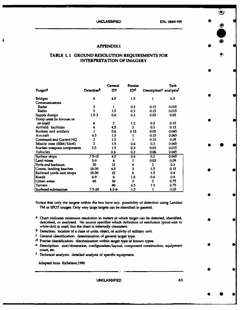
UNCLASSIFIED ERL-0694-RR
"APPENDIXI 0
TABLE L 1 GROUND RESOLUTION REQUIREMENTS FORINTERPRETATION OF IMAGERY
General Precis Tech
Targeta Detectionb IDc IDd Descriptione analysist
Bridges 6 4.5 1.5 1 0.3Commuunications
Radar 3 1 0.3 0.15 0.015Radio 3 1.5 0.3 0.15 0.015
Supply dumps 1.5-3 0.6 0.3 0.03 0.03Troop units (in bivouac oron road) 6 2 1.2 03 0.15
Airfield facilities 6 4.5 3 0.3 0.15Rockets and artillery 1 0.6 0.15 0.05 0.045Aircraft 4.5 1.5 1 0.15 0.045Command and Control HQ 3 1.5 1 0.15 0.09Missile sites (SSM/SAM) 3 1.5 0.6 0.3 0.045 * *Nuclear weapons components 2.5 1.5 0.3 0.03 0.015Vehicles 0.6 0.3 0.06 0.045Surface ships 7.5-15 4.5 0.6 0.3 0.045Land mines 3-9 6 1 0.03 0.09Ports and harbours 30 15 6 3 0.3Coasts, landing beaches 15-30 4.5 3 1.5 0.15Railroad yards and shops 15-30 15 6 1.5 0.4Roads 6-9 6 1.8 0.6 0.4Urban areas 60 30 3 3 0.75Terrain 90 4.5 1.5 0.75Surfaced submarines 7.5-30 4.5-6 1.5 1 0.03
Notice that only the targets within the box have any possibility of detection using LandsatTM or SPOT images. Only very large targets can be identified in general.
a Chart indicates minimum resolution in meters at which target can be detected, identified,described, or analysed. No source specifies which definition of resolution (pixel-size orwhite-dot) is used, but the chart is internally consistent.
b Detection: location of a class of units, object, or activity of military unit.c General identification: determination of general target type.d Precise identification: discrimination within target type of known types.e Description: size/dimension, configuration/layout, component construction, equipment 0
count, etc.f Technical analysis: detailed analysis of specific equipment.
Adapted from Richelson,1990
UNCLASSIFIED 63
* . 0
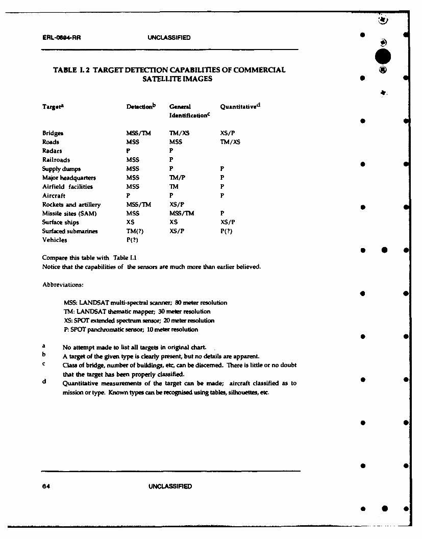
ERL-0604-RR UNCLASSIFIED 0
TABLE 1. 2 TARGET DETECTION CAPABILITIES OF COMMERCIALSATELLITE IMAGES 0
Targeta Djte0 gb General Quantitatived
Identificationc
Bridges MSS/TM TM/XS XS/PRoads MSS MSS TM/XSRadars P PRailroads MSS PSupply dumps MSS P PMajor headquarters MSS TM/P PAirfield facilities MSS TM PAircraft P P PRockets and artillery MSS/T`M XS/PMissile sites (SAM) MSS MSS/TM PSurface ships XS XS XS/PSurfaced submarines TM(?) XS/P P(?)Vehicles P(?)
Compare this table with Table 1.1Notice that the capabilities of the sensors are much more than earlier believed.
Abbreviations:
MSS: LANDSAT multi-spectral scanner; 80 meter resolutionTM: LANDSAT thematic mapper; 30 meter resolutionXS: SPOT extended spectrum sensor; 20 meter resolutionP: SPOT panchromatic sensor; 10 meter resolution
a No attempt made to list all targets in original chart.b A target of the given type is clearly present, but no details are apparent.c Class of bridge, number of buildings, etc, can be discerned. There is little or no doubt
that the target has been properly classified.d Quantitative measurements of the target can be made; aircraft classified as to
mission or type. Known types can be recognised using tables, silhouettes, etc.
64 UNCLASSIFIED

UNCLASSIFIED ERL-0694-RR -
4APPENDIX II
PIXELISATION EFFECT ON SHADOW WIDTH MEASUREMENT
In analytical terms the determination of width of a linear object can be achieved in manyways. One simple approach is to divide the area covered by the object by its length. Thisapproach can not be directly implemented in image processing for computing shadow widths.
In Figure 11.1 shadows are drawn as the area between pairs of lines. Widths are indicated
opposite to the pairs of lines. The surface is divided into 10xlO m grids to simulate SPOTrimage pixels. The black pixels are those in which 50% or more of the pixel area is covered byshadow. It is assumed that a perfect technique is available to threshold such pixels and labelthem as shadows.
Due to the discrete pixel sizes involved in images the shadow zones may appear as continuousareas or as fragments. Under perfect thresholding conditions, as described above, one can
expect continuous shadow zones only if the shadows have widths equal to or greater than thepixel dimensions.
* 0 =
From the figure it is also clear that the shadow width computed by dividing the area of
shadow pixels by the length needs to be corrected. For example, the area covered by the 10 m.wide shadow is 20 pixels or 2000 m 2 . The length of the shadow is 208.8 m. The computedwidth of the shadow is 9.58, which is less than 10 m. In order to get the correct estimate thelength must be measured along the scan line or the actual length must be multiplied by the
cosine of the angle between the shadow zone and the scan line.
U 0
UNCLASSIFIED 65
S.. . . . . . . . . . .. . . . . i l . . . . . . .. . I . .. . . . . . . . . . . . . . i i . .. . . . ri JJil IIi i i . . . . .* i . .. . . . .. . .
ERL-0694-RR UNCLASSIFIED 0 6
0
0
IB 0 01 m
* 0
14
shadow zone may be expected.
* 0
0 0
* 0
66 UNCLASSIFIED
- 0
UNCLASSIFIED ERL-0694-RR 0 6DISTRIBUTION
No of Copies
Defence Science and Technology Organilation
Chi Defence Scien)st
Central Office Executive ) I shared copy
Counsellor, Defence Science, London Cont Sht
Counsellor, Defence Sciene, Washington Cont Sht
Scientific Adviser POLCOM 1
Senior Defence Scientific Adviser IAssistant Secretary Scientific Analysis I
HQADF 0DGFD(L)
DIOImage Exploitation Centre
Navy Office
Navy Scientific Adviser 1 0
Air OfficeAir Force Scientific Adviser
Army OfficeScientific Adviser, Army
Electronics Research Laboratory 0Director 1Chief, Information Technology Division I
Chief, Communications Division Cont Sht
Chief, Electronic Warfare Division Cont Sht
Chief, Guided Weapons Division Cont Sht
Research Leader, Command & Control and Intelligence Systems I
Research Leader, Military Computing Systems I
Research Leader, Human Computer Interaction 1
Head, Program and Executive Support 1 0 0
Head, Command Support Systems Group I
Head, Intelligence Systems Group I
Head, Information Management Group 1
Head, Systems Simulation and Assessment Group 1
Head, Exercise Analysis Group 1 0 0Head, C3I Systems Engineering Group 1
Head, Software Engineering Group I
Head, Trusted Computer Systems Group I
Head, Computer Systems Architecture Group 1
Head, Information Acquisition & Processing Group 1 0 0
Mr V. K. Shettigara (Author) 1
Mr G. M. Sumerling (Author) I
Mr P.J. Whitbread (Author) 1
0
UNCLASSIFIED 67
* . 0
ERL-0694-RR UNCLASSIFIED
Publications & Publicity Officer, ITDSurveillance Research Laboratory
Director 1
Chief, Land Space and Optoelectronics Division 1
Libraries and Information Services
Australian Government Publishing Service I
Defence Central Library, Technical Reports Centre 1 I
Manager, Document Exchange Centre, (for retention) INational Technical Information Service, United States 2
Defence Research Information Centre, United Kingdom 2
Director Scientific Information Services, Canada IMinistry of Defence, New Zealand 1 0
National Library of Australia I
Defence Science and Technology Organisation Salisbury, Research Library 2Library Defence Signals Directorate 1
British Library Document Supply Centre I
MHQ S
MCAUST I
CSIRO Division of Water Resources
Dr D.LB.Jupp 1
USATEC
Dr M.B.Satterwhite 1I0Spares
Defence Science and Technology Organisation Salisbury, Research library 6
*0
* 0
* 0
68 UNCLASSIFIED
""i n 0

CDepartment of Defence 1. Page c ation 0
Unclassilied
DOCUMENT COW-ROL DATA SHEET 2. Pr dcy ument )et
3A. AR Numnbe 3b. Laboratory Number 3c. Type Report 4. Task Number
AR-008-137 ERL-0694-RR RESEARCH REPORT 0
5. Document Date 6. Cost Code 7. Security Classification 8. No. of Pages 76NOVEMBER 1903
10. Title E 9. oDocument Title Abstract
SOME DEFENCE APPLICATIONS OF CIVILIANREMOTE SENSING SATELLITE IMAGES S (Secrot) C (Confl) R (Rest) U (Unclass)
* For UNCLASSIFIED docs with a secondary distributionLIMITATION, use (L) In document box.
11. Author(s) 12. Downgrading/Deflmiting InstructonsVittala K. ShottigaraGordon M. Sumeding and NIAPaul J. Whitbread
13a. Corporate Author and Address 14. Officer/Position responsible for
Electronics Research Laboratory Security: ........... NIA ...........................................................PO Box 1500, Salisbury SA 5108
Downgrading:....N/A .....................................................13b. Task Sponsor Approval forRelease:...DERL ............................................
15. Secondary Release Statement of this Document
APPROVED FOR PUBLIC RELEASE
16a. Deliberate Announcement 0
No Limitation
1 6b. Casual Announcement (for citation in other documents)
[xl No Umitation Rot. by Author, Doc No. and dote only.
17. DEFTEST Descriptors 18. DISCAT Subject Codes
Remote senw gSatellite imagery 080201Image analysisMilitay applicationsMtaty inteulgece •
19. Abstract
This report is on a pilot study to demonstrate some of the capabilities of remote sensing in intelligencegathering. A wide variety of issues, both quantitative and qualitative, are addressed. SPOT satellite •images were used for object classification using statistical and neural net techniques, object heightdetermination and image resolution enhancement. A new procedure was developed for detecting smalland man-made objects in multispectral or colour images. The procedure will be presented in acompanion report.
18•ms 0oS@WFf