
Acoustic energy transfer · Dit proefschrift is goedgekeurd door de promotor. De samenstelling van...
202
Exploring the potential of acoustic energy transfer Roes, M.G.L. Published: 25/11/2015 Document Version Publisher’s PDF, also known as Version of Record (includes final page, issue and volume numbers) Please check the document version of this publication: • A submitted manuscript is the author's version of the article upon submission and before peer-review. There can be important differences between the submitted version and the official published version of record. People interested in the research are advised to contact the author for the final version of the publication, or visit the DOI to the publisher's website. • The final author version and the galley proof are versions of the publication after peer review. • The final published version features the final layout of the paper including the volume, issue and page numbers. Link to publication Citation for published version (APA): Roes, M. G. L. (2015). Exploring the potential of acoustic energy transfer Eindhoven: Technische Universiteit Eindhoven General rights Copyright and moral rights for the publications made accessible in the public portal are retained by the authors and/or other copyright owners and it is a condition of accessing publications that users recognise and abide by the legal requirements associated with these rights. • Users may download and print one copy of any publication from the public portal for the purpose of private study or research. • You may not further distribute the material or use it for any profit-making activity or commercial gain • You may freely distribute the URL identifying the publication in the public portal ? Take down policy If you believe that this document breaches copyright please contact us providing details, and we will remove access to the work immediately and investigate your claim. Download date: 17. Sep. 2018
Transcript of Acoustic energy transfer · Dit proefschrift is goedgekeurd door de promotor. De samenstelling van...

Exploring the potential of acoustic energy transfer
Roes, M.G.L.
Published: 25/11/2015
Document VersionPublisher’s PDF, also known as Version of Record (includes final page, issue and volume numbers)
Please check the document version of this publication:
• A submitted manuscript is the author's version of the article upon submission and before peer-review. There can be important differencesbetween the submitted version and the official published version of record. People interested in the research are advised to contact theauthor for the final version of the publication, or visit the DOI to the publisher's website.• The final author version and the galley proof are versions of the publication after peer review.• The final published version features the final layout of the paper including the volume, issue and page numbers.
Link to publication
Citation for published version (APA):Roes, M. G. L. (2015). Exploring the potential of acoustic energy transfer Eindhoven: Technische UniversiteitEindhoven
General rightsCopyright and moral rights for the publications made accessible in the public portal are retained by the authors and/or other copyright ownersand it is a condition of accessing publications that users recognise and abide by the legal requirements associated with these rights.
• Users may download and print one copy of any publication from the public portal for the purpose of private study or research. • You may not further distribute the material or use it for any profit-making activity or commercial gain • You may freely distribute the URL identifying the publication in the public portal ?
Take down policyIf you believe that this document breaches copyright please contact us providing details, and we will remove access to the work immediatelyand investigate your claim.
Download date: 17. Sep. 2018

Exploring the potential ofacoustic energy transfer
Maurice G. L. Roes

First edition, published 2015
Copyright © 2015 M. G. L. Roes
Printed by Gildeprint DrukkerijenCover design by M. G. L. Roes
All rights reserved. No part of this thesis may be reprinted orreproduced or utilised in any form or by any electronic, mechanical,or other means, now known or hereafter invented, includingphotocopying and recording, or in any information storage orretrieval system, without permission in writing from the author.
A catalogue record for this thesis is available from the EindhovenUniversity of Technology Library
ISBN: 978-90-386-3955-0

Exploring the potential ofacoustic energy transfer
PROEFSCHRIFT
ter verkrijging van de graad van doctor aan de TechnischeUniversiteit Eindhoven, op gezag van de rector magnificusprof. dr. ir. F. P. T. Baaijens, voor een commissie aangewezen
door het College voor Promoties, in het openbaar teverdedigen op woensdag 25 november 2015 om 16:00 uur.
door
Maurice Gijsbert Lodewijk Roes
geboren te Breukelen

Dit proefschrift is goedgekeurd door de promotor. De samenstelling van depromotiecommissie is als volgt:
voorzitter: prof. dr. ir. A. C. P. M. Backx1e promotor: prof. dr. E. A. Lomonovacopromotoren: dr. J. L. Duarte
ir. M. A. M. Hendrixleden: prof. dr. ir. R. M. Aarts
prof. dr. mont. M. Kupnik (TU Darmstadt)prof. dr. ir. I. Lopez Arteagaprof. E. M. Yeatman (Imperial College London)
Het onderzoek dat in dit proefschrift wordt beschreven is uitgevoerd inovereenstemming met de TU/e Gedragscode Wetenschapsbeoefening.
Summary
Exploring the potential of acoustic energy transfer
AHANDFUL OF METHODS for the contactless transfer of energy are availablenowadays. The most common of these is the use of inductively coupled coils,
which is already being used extensively in various consumer electronicsand in industrial applications. Less commonly encountered species of contactlessenergy transfer (CET) include capacitive coupling, far-field electromagnetic, optical,and, as a very recent development, acoustic systems. The last-mentioned form is themain topic of this thesis.
Acoustic energy transfer, or AET, is a method of contactless energy transfer thatmakes use of sound waves as an intermediate energy carrier to transfer energy. Atransmitter converts electrical energy into vibrations, which are successively radiatedas a pressure wave. The medium which it propagates in can be of a gaseous, fluid ora solid nature. A receiver at a point along the path of the sound wave extracts theenergy from the wave and converts it back into electrical energy. Unlike inductivelycoupled CET, acoustic energy transfer can transfer energy at a high efficiency overdistances that are large in comparison to the transmitter and receiver sizes, owingto the high directivity of the transmitter. The efficiency of inductive CET drops offsharply when the distance becomes larger than the coil diameter. Acoustic energytransfer has the additional advantage of not relying on electromagnetic fields forthe propagation of energy. Therefore it is ideally suited in situations where thesefields are undesirable; for instance in hazardous environments, in direct vicinity ofmetallic objects, or in environments where the presence of strong electromagneticfields is a health and safety issue.
This thesis is aimed at creating understanding of the workings of acoustic energytransfer in air. It starts from basic sound wave theory and through experimentsworks its way forward. Its main purpose lies in providing an exploratory overview ofthe subject, pointing out the main features, chances and limitations of the approach.
v

vi SUMMARY
It investigates a number of peculiarities of the system and describes various pathsthat have been followed in the pursuit of optimised system performance. Topics thatare covered are the theoretical limit to the energy transfer efficiency, determination oflosses, modelling of effects that are encountered during measurements, and designand implementation of impedance adaptation measures for transducers.
A model based on diffraction and attenuation predicts that energy transfer over adistance of one metre is possible at an efficiency of 65 %, when the diameter of thetransmitter and receiver is limited to 20 cm. Optimal electrical loading conditions,derived from this model, indicate that the receiving element has an efficiency of50 % when maximum output power is desired. Even when these transducer lossesare included in the model, acoustic energy transfer still performs at least five to tentimes better in terms of efficiency than an inductively coupled system of the samedimensions.
Experiments, in which a maximum output power of 40 mW was demonstrated,reveal the occurrence, influence and importance of reflections on the energy transferof an AET system. Reflections greatly boost the output power, but only at distinctdistances from the transmitter, thereby preventing free placement of the receivingelement. These reflections are modelled both by means of finite element modelling,and with a transmission line model in which a lumped element attenuation coef-ficient is used to account for spreading of the sound wave and absorption in themedium.
Impedance matching of the transmitting and receiving transducers to the medium isinvestigated as a means for increasing the output power and reducing the influenceof reflections on the energy transfer. Two methods of impedance adaptation areconsidered in this thesis. Stepped-exponential horns were designed, optimised andconstructed for both the transmitting and receiving transducers. Resonance in thehorns is used to obtain large impedance transformation ratios. Experiments showthat the horns increase the output power by a factor 3.1 and the efficiency by afactor 7.5 at 10 cm distance between the transmitter and the receiver. However, themodelled response deviates significantly from the measured behaviour. A secondimpedance adaptation measure was found in radiating surface enlargement. It isapplied to bolt-clamped Langevin transducers in the form of aluminium plates thatcan be screwed onto the transducer. It was found that the plates do not increasethe output power. Experiments also revealed significant nonlinearity of the trans-ducer output with respect to the driving voltage, resulting in chaotic behaviour. Amaximum output power of 36.3 mW was measured. It can be shown that optimalpositioning of the transmitter is possible based on measurements of its electricalimpedance.
This thesis shows that acoustic energy transfer through air is feasible. Achieved

SUMMARY vii
power levels are adequate for small systems such as sensors, MEMS, et cetera, butare insufficient for implementation in more power hungry applications such asactuators or wireless charging. The transducers are the restricting factor. Transducermodelling is shown to be of critical importance for accurate acoustic energy transferperformance, since it is the element that connects the electrical, mechanical andacoustic domains.


Contents
Summary v
1 Conventions 11.1 Symbols . . . . . . . . . . . . . . . . . . . . . . . . . . . . . . . . . . . 11.2 Acoustic impedance . . . . . . . . . . . . . . . . . . . . . . . . . . . . 21.3 Mathematical notation . . . . . . . . . . . . . . . . . . . . . . . . . . . 2
2 Introduction 52.1 Background . . . . . . . . . . . . . . . . . . . . . . . . . . . . . . . . . 6
2.1.1 Contactless energy transfer . . . . . . . . . . . . . . . . . . . . 62.1.2 Acoustic energy transfer . . . . . . . . . . . . . . . . . . . . . . 82.1.3 Acoustic energy transfer versus inductive CET . . . . . . . . . 10
2.2 Research on AET . . . . . . . . . . . . . . . . . . . . . . . . . . . . . . 112.3 Challenges . . . . . . . . . . . . . . . . . . . . . . . . . . . . . . . . . . 132.4 Research goals and outline of the thesis . . . . . . . . . . . . . . . . . 14
2.4.1 Research goals . . . . . . . . . . . . . . . . . . . . . . . . . . . 142.4.2 Outline of the thesis . . . . . . . . . . . . . . . . . . . . . . . . 15
3 A short introduction to acoustics 173.1 Sound waves . . . . . . . . . . . . . . . . . . . . . . . . . . . . . . . . . 173.2 Particles, pressure and sound velocity . . . . . . . . . . . . . . . . . . 18
3.2.1 The equation of state . . . . . . . . . . . . . . . . . . . . . . . . 193.2.2 The continuity equation . . . . . . . . . . . . . . . . . . . . . . 203.2.3 Euler’s equation . . . . . . . . . . . . . . . . . . . . . . . . . . 213.2.4 The wave equation . . . . . . . . . . . . . . . . . . . . . . . . . 22
3.3 Simple types of sound waves . . . . . . . . . . . . . . . . . . . . . . . 233.3.1 Plane waves . . . . . . . . . . . . . . . . . . . . . . . . . . . . . 233.3.2 Spherical waves . . . . . . . . . . . . . . . . . . . . . . . . . . . 24
ix
x CONTENTS
3.4 Attenuation of sound . . . . . . . . . . . . . . . . . . . . . . . . . . . . 263.5 Power and sound intensity . . . . . . . . . . . . . . . . . . . . . . . . . 27
3.5.1 Sound intensity . . . . . . . . . . . . . . . . . . . . . . . . . . . 273.6 Equivalent electrical networks . . . . . . . . . . . . . . . . . . . . . . . 30
4 First steps in acoustic energy transfer 334.1 Diffraction and attenuation . . . . . . . . . . . . . . . . . . . . . . . . 35
4.1.1 Diffraction . . . . . . . . . . . . . . . . . . . . . . . . . . . . . . 354.1.2 Attenuation . . . . . . . . . . . . . . . . . . . . . . . . . . . . . 424.1.3 Combined energy transfer efficiency . . . . . . . . . . . . . . . 454.1.4 Optimisation . . . . . . . . . . . . . . . . . . . . . . . . . . . . 47
4.2 Transducer efficiency . . . . . . . . . . . . . . . . . . . . . . . . . . . . 484.3 Experimental verification of the model . . . . . . . . . . . . . . . . . . 58
4.3.1 Parameter identification . . . . . . . . . . . . . . . . . . . . . . 584.3.2 Setup . . . . . . . . . . . . . . . . . . . . . . . . . . . . . . . . . 644.3.3 Measurement results . . . . . . . . . . . . . . . . . . . . . . . . 65
4.4 Conclusions and discussion . . . . . . . . . . . . . . . . . . . . . . . . 69
5 Reflections 735.1 Transmission line models . . . . . . . . . . . . . . . . . . . . . . . . . 74
5.1.1 Pressure and impedance . . . . . . . . . . . . . . . . . . . . . . 755.1.2 Power and efficiency . . . . . . . . . . . . . . . . . . . . . . . . 765.1.3 Location of peaks . . . . . . . . . . . . . . . . . . . . . . . . . . 775.1.4 Attenuation coefficient . . . . . . . . . . . . . . . . . . . . . . . 785.1.5 Simulation results . . . . . . . . . . . . . . . . . . . . . . . . . 805.1.6 Parameter fitting . . . . . . . . . . . . . . . . . . . . . . . . . . 84
5.2 Finite element modelling . . . . . . . . . . . . . . . . . . . . . . . . . . 885.2.1 Results . . . . . . . . . . . . . . . . . . . . . . . . . . . . . . . . 905.2.2 Parameter sensitivity . . . . . . . . . . . . . . . . . . . . . . . . 94
5.3 Conclusions and discussion . . . . . . . . . . . . . . . . . . . . . . . . 97
6 Horns 1016.1 Waveguides . . . . . . . . . . . . . . . . . . . . . . . . . . . . . . . . . 1026.2 Exponential horns . . . . . . . . . . . . . . . . . . . . . . . . . . . . . . 103
6.2.1 Infinite horns . . . . . . . . . . . . . . . . . . . . . . . . . . . . 1046.2.2 Horns of finite length . . . . . . . . . . . . . . . . . . . . . . . 105
6.3 Introductory measurements . . . . . . . . . . . . . . . . . . . . . . . . 1086.3.1 Results . . . . . . . . . . . . . . . . . . . . . . . . . . . . . . . . 108
6.4 Stepped-exponential horns . . . . . . . . . . . . . . . . . . . . . . . . . 1116.4.1 Transducer losses . . . . . . . . . . . . . . . . . . . . . . . . . . 1136.4.2 Experimental results . . . . . . . . . . . . . . . . . . . . . . . . 1146.4.3 Differences between measurements and simulations . . . . . 116

CONTENTS xi
6.5 Conclusions and discussion . . . . . . . . . . . . . . . . . . . . . . . . 129
7 Experiments with bolt-clamped Langevin transducers 1337.1 Reflections . . . . . . . . . . . . . . . . . . . . . . . . . . . . . . . . . . 1347.2 Normal modes . . . . . . . . . . . . . . . . . . . . . . . . . . . . . . . . 1377.3 Load impedance . . . . . . . . . . . . . . . . . . . . . . . . . . . . . . . 1387.4 Comparison between plate dimensions . . . . . . . . . . . . . . . . . 1407.5 Nonlinearity . . . . . . . . . . . . . . . . . . . . . . . . . . . . . . . . . 1417.6 Energy transfer . . . . . . . . . . . . . . . . . . . . . . . . . . . . . . . 146
7.6.1 Variation of distance . . . . . . . . . . . . . . . . . . . . . . . . 1467.6.2 Variation of input voltage . . . . . . . . . . . . . . . . . . . . . 148
7.7 Reproducibility . . . . . . . . . . . . . . . . . . . . . . . . . . . . . . . 1507.8 Conclusions and discussion . . . . . . . . . . . . . . . . . . . . . . . . 153
8 Conclusions & recommendations 1598.1 Conclusions . . . . . . . . . . . . . . . . . . . . . . . . . . . . . . . . . 1598.2 Thesis contributions . . . . . . . . . . . . . . . . . . . . . . . . . . . . 1618.3 Recommendations . . . . . . . . . . . . . . . . . . . . . . . . . . . . . 163
A Symbols and notation 169A.1 Symbols . . . . . . . . . . . . . . . . . . . . . . . . . . . . . . . . . . . 169A.2 Subscripts and superscripts . . . . . . . . . . . . . . . . . . . . . . . . 170A.3 Notation . . . . . . . . . . . . . . . . . . . . . . . . . . . . . . . . . . . 171A.4 Acronyms . . . . . . . . . . . . . . . . . . . . . . . . . . . . . . . . . . 171A.5 Physical constants . . . . . . . . . . . . . . . . . . . . . . . . . . . . . . 172
B Coordinate systems 173B.1 Coordinate transformations . . . . . . . . . . . . . . . . . . . . . . . . 173
B.1.1 Spherical coordinates . . . . . . . . . . . . . . . . . . . . . . . . 173B.1.2 Cylindrical coordinates . . . . . . . . . . . . . . . . . . . . . . 173
B.2 Gradient . . . . . . . . . . . . . . . . . . . . . . . . . . . . . . . . . . . 174B.2.1 Gradient in spherical coordinates . . . . . . . . . . . . . . . . . 174B.2.2 Gradient in cylindrical coordinates . . . . . . . . . . . . . . . . 175
References 177
Acknowledgements 187
About the author 189

CH
AP
TE
R
1 Conventions
SEVERAL conventions have been adopted in this thesis, some of which willbe familiar to the reader, while others may not be so obvious at first glance.To avoid any ambiguity in meaning and understanding of notations and
symbols, the notational conventions that are employed are discussed in this chapter.A complete list of symbols and notation is added in Appendix A at page 169 for thereader’s reference, in which all symbols and notation are grouped in tables for easyreference.
1.1 Symbols
Considering that the work described in this dissertation deals with two differentdomains of engineering, i.e. the electrical and the mechanical or acoustical domain,there will inevitably be some overlap in the traditional symbol definitions of certainquantities. For example, both mechanical speed and electrical voltage are normallyindicated with a small v or the capital V. To allow a distinction between the twovariables to be made, in this thesis voltages are always indicated with a v and themechanical speed is expressed as u. Likewise, pressure is represented by a small p,and pressure amplitude by P, not to be confused with power, which will always beindicated with a capital Π.
As mentioned earlier, the reader is kindly referred to Appendix A in case of anydoubt with respect to the meaning of certain variables or parameters.
1

2 CHAPTER 1 CONVENTIONS
1.2 Acoustic impedance
Although the concept of impedance was introduced by Oliver Heaviside in 1886, itwas only in 1919 that the term was first used in connection with acoustic problemsby Arthur Webster [128]. While originally the term ‘impedance’ implied a quantitythat impedes or restricts current flow, a more accurate description would be thatimpedance impedes the flow of energy. This broader definition allows the concept tobe used in acoustics just as well as in electric problems.
Although Webster originally proposed to define the acoustic impedance as the ratioof the excess pressure p to the volume displacement X in the medium; Za = p/X, thisdefinition is far from definite. Most works on acoustics define acoustic impedanceas pressure divided by volume velocity (for example [58, 85, 120]) although otherdefinitions exist, such as pressure divided by particle velocity (e.g. [57, 69]). Lastly,the radiation impedance of a vibrating object is typically defined in the same manneras a mechanical impedance, that is, as the ratio of force to velocity.
Obviously, each of these definition has its own merits. Electing the volume velocity tobe an equivalent of current allows to make use of continuity relationships. Choosingforce, on the other hand, as equivalent of voltage and velocity for current meansthat the power relationship of the equivalent circuit is maintained. Moreover, thischoice has the advantage that it is the definition of mechanical impedance, whichconveniently expresses the radiation impedance of a loudspeaker for example.In this dissertation, however, acoustic impedance is defined as the quotient ofpressure and particle velocity. Since this work uses the excess pressure and particlevelocity as principal acoustical quantities, it is only logical to choose these quantitiesas equivalents for voltage and current respectively. Moreover, specific acousticimpedance of a medium has the same definition [58]. The resulting unit of acousticimpedance is N s/m3, for which often the Rayleigh or rayl unit is used.
1.3 Mathematical notation
Vectors represent quantities that do not only have a magnitude, but that also have adirection. This directional dependency is indicated in this thesis by an arrow abovethe symbol, so as to be able to distinguish them from scalar quantities, for examplethe vector ~x, as opposed to the scalar x.
Special spatial derivatives of vector fields such as the gradient, divergence and curlare denoted using∇, the ‘nabla’ or ‘del’ operator. It is defined in the Euclidian spacewith coordinates (x1, x2, . . . , xn) and unit vectors x1, x2, . . . xn in the corresponding

1.3 MATHEMATICAL NOTATION 3
directions, as
∇ =n
∑i=1
xi∂
∂xi. (1.1)
For a standard three-dimensional Cartesian coordinate system with unit vectors x, yand z this would be
∇ = x∂
∂x+ y
∂
∂y+ z
∂
∂z. (1.2)
According to this notation, the gradient of a scalar field s, and the divergence andcurl of a vector field ~v = vx x + vyy + vz z are respectively given by
∇s =∂s∂x
x +∂s∂y
y +∂s∂z
z (1.3a)
∇ ·~v =∂vx
∂x+
∂vy
∂y+
∂vz
∂z(1.3b)
∇×~v =
(∂vz
∂y−
∂vy
∂z
)x +
(∂vx
∂z− ∂vz
∂x
)y +
(∂vy
∂x− ∂vx
∂y
)z (1.3c)
Lastly, complex quantities are denoted by means of a bar notation, for examplea = α+ jβ. Complex variables are frequently used throughout this thesis to representharmonically varying quantities.


CH
AP
TE
R
2 Introduction
ENERGY is a truly elusive physical property. It is something that cannot beobserved directly, although one can observe the effects energy brings about—itcan be felt as heat, experienced as velocity, seen and heard as lightning and
thunder, or the crashing of waves onto the shore. This is probably the main reasonfor many people finding it so fascinating a concept. It is shrouded in a bit of magicand mystery, in a world that is thoroughly dissected, classified and (arguably) largelyunderstood.
Energy is often described as the ability of a system to perform work. Now work is amuch more comprehensible concept for most people. Mechanical work is performedwhen a force is exerted on an object in order to move it. More precisely: the productof the force in the direction of the movement, multiplied by the distance travelled,equals the mechanical work done.
Energy exists in many forms: electrical, mechanical, thermal, nuclear, magnetic,gravitational, chemical, et cetera. Mankind has used many of these forms of en-ergy throughout history. Mechanical, thermal and chemical energy have long beenthe energies of choice. Starting with the industrial revolution the use of energyskyrocketed, and has continued its growth ever since. The advent of the electricalera, starting from around the mid-1880s, brought a whole new source of energywithin reach of the common man. It meant constantly available lighting without the
This chapter is based on [96] and [97].
5
6 CHAPTER 2 INTRODUCTION
disadvantages of fire hazard, smell and smoke, all at the command of a button. Nu-merous applications would follow, leading to the present day world were electricalenergy plays such a vital role that the whole society would collapse if the powersystem were to fail. Man embraced electricity as its main energy carrier, not only inhis home, but for his portable devices as well. The amount of comfort and luxuryexperienced because of this choice is unrivalled throughout history.
One of the inherent drawbacks of electricity, albeit a negligible one in most cases, isthe fact that a physical connection is necessary for the electrical energy to propagate.Wire connections are a necessity for electric currents to flow efficiently from one pointto the other. As a result, copper must have never been in so high a demand since theend of the bronze age around 1200BCE, relatively speaking. The requirement of aphysical connection can be somewhat alleviated through the use of a battery as apower source, as is extremely common nowadays in portable devices, such as mobilephones, cameras, laptop computers, et cetera. Recharging of these batteries, however,still requires a connection to another source of electrical energy. Contactless energytransfer (CET) has been envisaged by many to overcome the necessity of a physicalconnection between an electrical energy source on one hand, and an electrical deviceon the other hand. Some even dreamt dreams as bold as powering a whole worldwirelessly [1].
There are many applications were a physical connection between a device and apower source is impractical or even impossible. In other cases it may only be amatter of convenience. Contactless energy transfer is used to charge the batteriesof mobile devices or vehicles [119, 126], it is used in industry to power actuators inwhich the disturbance force introduced by a cable slab is undesired [23, 118], it canbe used to charge implants without surgical intervention [25,88], or it can be used topower sensor networks [55].
2.1 Background
2.1.1 Contactless energy transfer
A handful of methods for the contactless transfer of energy are available nowadays.The most common of these is the use of inductively coupled coils, a coreless trans-former if you will, which is being used already in various consumer electronics andin industrial applications. Less commonly encountered species of CET include capa-citive coupling, far-field electromagnetic, optical, and, as a very recent development,acoustic systems. The last-mentioned form is the main topic of this thesis. Figure2.1 schematically depicts the working area of these methods of contactless energy
2.1 BACKGROUND 7
Frequency (log) →
Dis
tanc
e(l
og)→
Acoustic
Capacitive
Inductive
Microwave
Optical
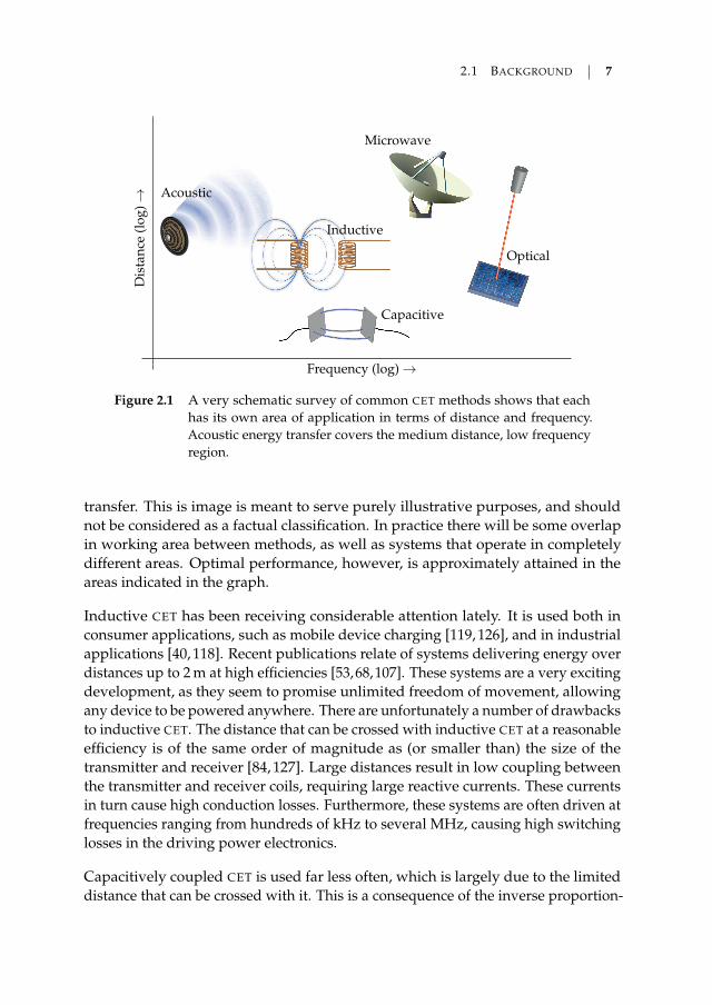
Figure 2.1 A very schematic survey of common CET methods shows that eachhas its own area of application in terms of distance and frequency.Acoustic energy transfer covers the medium distance, low frequencyregion.
transfer. This is image is meant to serve purely illustrative purposes, and shouldnot be considered as a factual classification. In practice there will be some overlapin working area between methods, as well as systems that operate in completelydifferent areas. Optimal performance, however, is approximately attained in theareas indicated in the graph.
Inductive CET has been receiving considerable attention lately. It is used both inconsumer applications, such as mobile device charging [119, 126], and in industrialapplications [40, 118]. Recent publications relate of systems delivering energy overdistances up to 2 m at high efficiencies [53,68,107]. These systems are a very excitingdevelopment, as they seem to promise unlimited freedom of movement, allowingany device to be powered anywhere. There are unfortunately a number of drawbacksto inductive CET. The distance that can be crossed with inductive CET at a reasonableefficiency is of the same order of magnitude as (or smaller than) the size of thetransmitter and receiver [84, 127]. Large distances result in low coupling betweenthe transmitter and receiver coils, requiring large reactive currents. These currentsin turn cause high conduction losses. Furthermore, these systems are often driven atfrequencies ranging from hundreds of kHz to several MHz, causing high switchinglosses in the driving power electronics.
Capacitively coupled CET is used far less often, which is largely due to the limiteddistance that can be crossed with it. This is a consequence of the inverse proportion-
8 CHAPTER 2 INTRODUCTION
ality of the capacitance with the distance, requiring high voltages and frequenciesfor the transfer of a reasonable amount of energy. High voltages lead to difficulties inprevention of electric breakdown. The advantage of capacitively coupled contactlessenergy lies in the nature of the electric field, which, unlike the magnetic field used ininductive CET, is much more constrained between the metal plates. As such there areless electromagnetic compatibility issues to be expected [55]. The high frequencies,on the other hand, may completely negate this advantage.
Far-field electromagnetic (EM) energy transfer, [16, 28, 81], often called RF energytransfer or microwave energy transfer, is used occasionally for contactless energytransfer as well. In contrast to inductive and capacitive energy transfer, far-fieldCET, as the name implies, uses a radiative electromagnetic field to convey energy.Hence microwaves and directional antennas have to be used. Both the transmitterand receiver size will at least be of the order of a wavelength, if they are to havea certain directivity. Consequently, when system dimensions lie in the centimetrerange, frequencies of the order of 10 GHz are necessary. Rectification of these highfrequency waves at the receiving end can be achieved at high efficiencies of 80 %–90 % [81], but generation of the microwaves is much more difficult, especially whena solid-state RF generator is used.
Optical energy transmission uses the same principle as far-field EM but here thewavelengths lie in (or near) the visible spectrum. Lasers can be used to generatethe optical beam, and photovoltaic diodes can take care of the conversion back toelectrical energy [28, 93, 104]. So far, in both conversion steps between 40 and 50 %of energy is lost [28]. Furthermore, the possible risks and hazards involved in theuse of high power laser beams should not be underestimated [45, 104].
2.1.2 Acoustic energy transfer
All of the previously described methods rely on electromagnetic fields for the transferof energy. One can divide them into energy transfer based on radiative (microwaveand optical CET) and nonradiative fields (inductive and capacitive CET). The formertype of energy transfer is not restricted to the use of electromagnetic waves alone;any type of wave can be used for this purpose. The transport of energy by soundwaves instead of EM waves lies at the basis of acoustic energy transfer (AET).
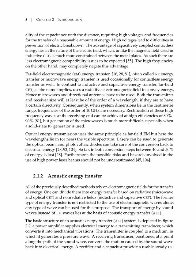
The basic structure of an acoustic energy transfer (AET) system is depicted in figure2.2; a power amplifier supplies electrical energy to a transmitting transducer, whichconverts it into mechanical vibrations. The transmitter is coupled to a medium, inwhich it generates a pressure wave. A receiving transducer, positioned at a pointalong the path of the sound wave, converts the motion caused by the sound waveback into electrical energy. A rectifier and a capacitor provide a usable steady DC
2.1 BACKGROUND 9
poweramplifier rectifier load
transmittingtransducer
receivingtransducer
medium
Figure 2.2 An acoustic energy transfer system consists of a transmitting trans-ducer that generates sound waves in a medium, and a receiving trans-ducer that converts them back to electrical energy.
voltage that powers a load. The medium can be anything ranging from air to humantissue or a solid; in principle any material that will propagate a pressure wave willdo.
Acoustic energy in its purest form is used in various applications, such as ultrasoniccleaning, medical ultrasonography, nondestructive testing, distance measurement(e.g. sonar), therapeutic ultrasound, ultrasonic welding, et cetera. These applicationsare different from acoustic energy transfer in that they directly use the acousticenergy for a specific purpose, without converting it back to electrical energy. Some-what closer related to AET are piezoelectric energy harvesting and piezoelectrictransformers. Energy harvesters make use of available (vibrational) energy to gener-ate electricity, and could be considered to be a non-driven AET system. Piezoelectrictransformers convert electric energy into vibrations, with the inverse process takingplace at the secondary side, which is the essence of AET. However, it lacks thespatial separation of the transmitter and receiver that is desired for a contactlessenergy transfer system. The ceramic of such a transformer is transmitter, receiverand medium, all in one.
One of the advantages of acoustic energy transfer, in comparison to CET based onelectromagnetic fields, lies in the much lower speed of propagation c of pressurewaves in air with respect to the electromagnetic propagation velocity cEM. Therefore,the sound waves have a smaller wavelength for a given frequency than their electro-magnetic counterpart. This in turn means that the transmitter and receiver can be afactor cEM/c smaller for a given directionality of the transmitter [25]. Alternatively, ifthe desired transmitter and receiver dimensions are given (as is usually the case),then the frequency that is used in an AET system can be a factor cEM/c smaller thanthat of the electromagnetic system, while still achieving the same directionality.

10 CHAPTER 2 INTRODUCTION
Accordingly, losses in the driving power electronics will be much lower. The designof the electronics can be kept considerably simpler as well. Furthermore, becauseacoustic energy transfer, in contrast to all other discussed methods, does not relyon electromagnetic fields for the propagation of energy, it is ideally suited for situ-ations where these fields are undesired, for instance in hazardous environments,in direct vicinity of metallic objects, or environments where the presence of strongelectromagnetic fields is a health and safety issue.
2.1.3 Acoustic energy transfer versus inductive CET
The major competitor for acoustic energy transfer is of course inductively coupledCET, being the de facto standard at this moment. Well designed systems can reachtotal energy transfer efficiencies, including electronics, of over 95 %. However,when the distance between the transmitter and receiver becomes much larger thantheir radii, the efficiency of inductive CET decreases rapidly [127]. Mur-Miranda etal. [84] presented a simplified model of inductive contactless energy transfer thatindicates that the efficiency decreases with the sixth power of distance. The model byWaffenschmidt and Staring [127] shows that the efficiency of an inductively coupledsystem can be very high, even when using coils that have a low quality factor, butonly up to a certain distance. The graphs of efficiency versus distance that theypresent in their paper show a relatively flat efficiency curve up to a bending point,after which the efficiency drops sharply.
Acoustic energy transfer performs much better in this respect [25,78,98] and can be agood alternative when inductive CET falls short. It benefits from the focusing abilityof sound waves. The energy contained in the waves can therefore stay confined to anarrow beam, without too much divergence. In the ideal case the sound beam doesnot diverge at all, and the only losses in the propagation are due to absorption bythe medium. Chapter 4 will go into more detail about modelling of the losses in anAET system and derivation of a theoretical limit to the energy transfer efficiency.
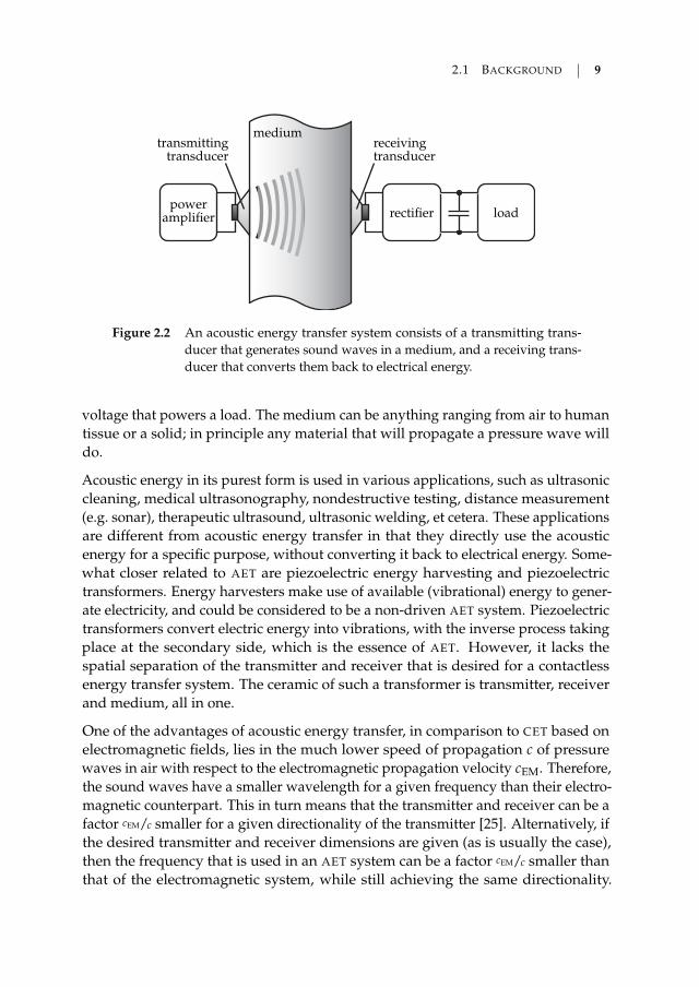
Figure 2.3 shows an example of how acoustic energy transfer is able to outperforminductive CET. The two methods are compared based on the celebrated paper byKurs et al. [68]. The paper describes an inductive energy transfer system using twoself-resonant coils of 30 cm radius, which were used to transfer 60 W over a distanceof more than 2 m at an efficiency of 40 %. The measured energy transfer efficienciesare indicated by the black dots in figure 2.3. As can be seen, they correspondquite well to the theoretical limit, reproduced from [127]. The point where themeasured efficiency starts to decrease occurs at a higher distance between the coils,but the drop in efficiency is just as sharp as predicted by Waffenschmidt and Staring.

2.2 RESEARCH ON AET 11
Theoretical limit AET
Theoretical limit ICET
Measurements ICETη
(−)→
zd (m) →
0 0.5 1 1.5 2 2.5 3 3.5 4 4.5 50
0.1
0.2
0.3
0.4
0.5
0.6
0.7
0.8
0.9
1
Figure 2.3 The measured efficiency η versus distance zd of an inductive CET
system from [68] shows a good resemblance with the theoretical limitfrom [127]. For larger distances the theoretical efficiency limit of anAET system of the same dimensions is much higher.
The theoretical efficiency limit for an acoustic energy transfer system1 of the samedimensions (i.e. a transmitter and receiver radius of 30 cm) shows the advantagethat AET has at larger distances. The efficiency decreases much more gradually, andoutperforms the inductive system when the distance becomes greater than 1.5 m.A typical operating frequency of 20 kHz was assumed for the AET system. Theefficiency of the AET system will be even higher when the frequency is optimised foreach distance.
This example illustrates the much reduced dependency on distance of acousticenergy transfer in comparison to inductive energy transfer. AET is therefore agood alternative whenever the distance to be crossed is larger than the size of thetransmitter and the receiver.
2.2 Research on AET
Acoustic energy transfer is not a new concept. The first application of AET datesback thirty years, to 1985, when Cochran et al. described a piezoelectric implant usedfor osteogenesis [19]. Their implant was a bit different from what was common atthat time, as it could be powered by a low intensity ultrasound source, making it the
1This efficiency limit is discussed in chapter 4.

12 CHAPTER 2 INTRODUCTION
first application of AET. After this publication it was silent for a long time aroundthe topic of AET. There was still only a handful of publications available on acousticenergy transfer at the time of the start of the research that is described in this thesis.At the present moment, however, the subject is starting to gain some momentum,and the number of publications on the topic slowly but steadily increases. Manyresearch groups in various parts of the world picked up the research topic, not inthe least due to publications of the author, notably [97].
Examining the limited amount of literature that exists on acoustic energy transfer,one can divide all publications into three groups on the basis of the propagationmedium that they use: fluid, metal, or air. The first two groups are by far the largest,while the number of publications on acoustic energy transfer through air is fairlylimited.
Fluid medium or tissue
Many publications on acoustic energy transfer deal with biomedical applications,where it is either used to power implants [9,25,54,70,72,73,78,80,88–91,108–112,114,115], or the energy of the ultrasonic wave is used directly for the intended purposewithout intermediate conversion to electrical energy [19, 26, 27].
At the moment batteries make up the largest part of the volume of an implant [25]. Inan attempt to miniaturise the implants, wireless energy transfer is proposed, so thatthe battery capacity can be reduced. An additional advantage of implant chargingby means of CET is that recharging is rendered a less invasive procedure. Acousticenergy transfer is a good alternative to inductive CET in this case because of theabsence of electromagnetic fields and the possibility of using a miniature receiver.Besides in vitro experiments, a number of authors have already shown the feasibilityof biomedical AET with in vivo experiments [70, 78].
As the characteristic impedance of tissue is very comparable to that of water, of-tentimes experiments are conducted in a fluid medium, instead of using actualtissue. The frequencies that are used in most publications lie in the megahertz range(0.5–2.25 MHz). Ozeri et al. explain that the choice of frequency for a biomedical AET
system is a trade-off between attenuation losses, diffraction losses, and additionallythe receiving transducer’s thickness [88].
The maximum efficiency that was measured in these publications is 39.1 % [90]. Thepower levels that are used are quite low (ranging from 29 µW to 100 mW electricaloutput power), which is limited by the allowable ultrasound intensity in in vivoapplications, in combination with a small receiver size. This level is adequate for thepower supply of, for instance, a simple sensor and its supporting signal processing.

2.3 CHALLENGES 13
Through-wall CET for metal enclosures
There are situations in which one would like to transfer energy wirelessly througha metal wall. Examples that come to mind are sensors in nuclear waste contain-ers, gas cylinders, vacuum chambers, pipelines, et cetera. Basically any systemqualifies where direct feed through of wires would severely complicate systemdesign, degrade the system’s performance, or is plainly impossible. Any formof CET based on electromagnetic fields runs into a wall here, quite literally. Themetal wall of such an enclosure has a shielding effect that limits the coupling ofan electromagnetic CET system and eddy currents in the wall cause high losses.Multiple authors have therefore proposed to use acoustic energy transfer as analternative [10, 43, 47, 48, 59, 71, 74, 76, 113, 116, 130, 131]. It is debatable whether thiscategory falls under the umbrella of CET, since it is not strictly a contactless method,but it is acoustic energy transfer nonetheless.
Through-wall AET achieves high output power levels and efficiencies more easilythan it does with an air or tissue medium, because of the similarity in acousticimpedance between the wall and piezoceramic material (approximately 45 Mraylfor steel and 30 Mrayl for lead zirconate titanate (PZT)). A good match in impedanceimplies optimal power throughput.
In [71] a through-wall acoustic energy transfer system is described that delivers50 W at 51 % efficiency. Leung et al. transferred 62 W at 74 % efficiency, while Bao etal. [10] even managed to transfer more than 1 kW at an efficiency of 84 % by using aprestressed piezo actuator.
Air
The combination of acoustic energy transfer with a gaseous medium [18, 50, 60, 98–100] is far less popular than biomedical or through-wall acoustic energy transferare. In [98] it was shown theoretically that AET has the potential of reaching highefficiencies in comparison with inductively coupled CET. The maximum efficiencythat was measured was 17 % and the transferred power was very low (4 µW). Itshould be noted that the authors indicated that the measurements were performedwith a non-optimised system and are meant to be nothing more than indicative.
2.3 Challenges
As mentioned, very few publications were available on acoustic energy transfer atthe moment that the research was initiated. The lack of preceding research puts it

14 CHAPTER 2 INTRODUCTION
in an unique position, making it true pioneering work. Unfortunately, it makes ita bit more difficult to give an overview of challenges than it is in well-establishedresearch fields.
Of the publications on AET that were available at the start of the research, onlya handful takes an analytical approach, or even attempts to construct a model ofacoustic energy transfer at all. None of these were meant for air-based acousticenergy transfer. Modelling is therefore one of the main challenges. Accurate modelsof the energy transfer in an acoustic energy transfer system will give fundamentalinsight into all effects that dominate AET behaviour. Models allow the right designchoices to be made to optimise the energy transfer and efficiency. Finite elementmodelling could prove a useful tool in giving a comprehensive overview of theeffects at play. Various existing models can possibly be combined to come up with amore comprehensive description of AET.
Overall, the thus far obtained output power levels in acoustic energy transfer arelow. In air based systems only microwatt levels were reached. While this can beenough to power a very simple sensor, higher levels are desirable if acoustic energytransfer is to become a serious competitor for inductively coupled CET. Transducerdesign is therefore deemed a subject that deserves much attention as well. Highpower transducers have already been developed by Bao et al., amongst others, forthrough-wall AET, while biomedical AET does not require high power levels dueto health regulations. Acoustic energy transfer through air, however, asks for atransducer design that is able to boost the received power to at least the level ofmultiple Watts.
This thesis is aimed at creating understanding of the workings of acoustic energytransfer in air. It starts from basic sound wave theory and simple initial experiments,and works its way forward from there. Topics that are covered are a theoretical limitto the energy transfer efficiency, determination of losses, modelling of effects that areencountered during measurements, and design and implementation of impedanceadaptation measures for transducers.
2.4 Research goals and outline of the thesis
2.4.1 Research goals
Inductively coupled systems are able to transfer energy very efficiently over shortdistances, but as soon as the distance becomes of the order of the size of the coils,the efficiency plummets. The obvious question to ask is whether acoustic energy
2.4 RESEARCH GOALS AND OUTLINE OF THE THESIS 15
transfer can outperform these systems in such a case. The research therefore is aimedat investigating the feasibility of acoustic energy transfer through air, and findingout how it stacks up against contactless energy transfer through inductively coupledcoils. To this end it is necessary to set up (multiphysical) models of the energytransfer by sound waves. Measurements on experimental setups are required, sothat the models can be validated.
If acoustic energy transfer is found to be a viable method for the transfer of energy,there are several secondary questions to be answered:
• What are characteristic properties of an acoustic energy transfer system, andhow can these be modelled?
• What is the limit to the power that can be transferred with a particular system,and what is the maximum efficiency that can be attained?
• What are the limiting factors in that case?
• How can the energy transfer and efficiency be increased?
It is important that the outcomes of the research have practical value, which isachieved by choosing a realistic set of requirements. The coils used in the inductiveCET system of Kurs et al., for example, are very large at a diameter of 60 cm. Theirapplication will therefore be incredibly limited. Because the purpose of contactlessenergy transfer is to power mobile devices, a transmitter and receiver size shouldbe chosen that reflect this mobility. The transmitter and receiver are thereforerestricted to a maximum cross-sectional diameter of 20 cm in this research. Sinceacoustic energy transfer is expected to perform much better than inductively coupledsystems at distances that are large in comparison to the transmitter and receiverdimensions, the goal is set to transfer energy efficiently over a distance of 1 m. Thisis a distance that allows a considerable freedom in device mobility, if it is poweredcontactlessly, and will certainly be of interest for many applications.
The power transfer efficiency of an inductively coupled CET system of the samedimensions will be taken as a benchmark. According to [127] such a system is ableto reach approximately 2 % efficiency, although only in very favourable conditions,i.e. a coil quality factor of 1000 and neglecting the losses in the accompanying powerelectronics. Furthermore, the high frequencies involved introduce many difficultiesin the design of an efficient inverter [122].
2.4.2 Outline of the thesis
The outline of this thesis is as follows. Chapter 3 starts with a short introductionto acoustics for the reader that is not yet familiar with this fascinating domain of
16 CHAPTER 2 INTRODUCTION
physics. The research, and especially the models, described in this thesis lean heavilyon the theory of acoustic wave propagation, making it imperative to have a grasp ofbasic acoustic concepts. The relations and equations, as well as simple wave types,are discussed briefly. The chapter also introduces the concept of equivalent electricalnetworks.
The first theory of acoustic energy transfer in air is subsequently discussed in chapter4. A theoretical limit to the energy transfer efficiency of an AET system is derived,and used to calculate the maximum attainable efficiency. Optimal electrical loadingconditions for the receiving transducer are derived. First experiments are discussedand compared to the theoretical limit. To this end transducer losses are determinedfrom vacuum impedance measurements.
The modelling of reflections in acoustic energy transfer systems is successivelytreated in chapter 5. A transmission line model that models the energy transfer bymeans of plane waves is introduced. Power and efficiency equations are derived andcompared to measurements. Finite element analysis is used to construct a secondmodel, which gives more insight into the pressure distribution at various transmitter-receiver distances. Sensitivity analysis is used to identify the most important modelparameters.
The next two chapters are dedicated to impedance adaptation measures. Chapter6 deals with the use of horns in acoustic energy transfer, for adjustment of theimpedance of both the transmitter and the receiver. Stepped-exponential horns aredesigned and optimised by means of finite element analysis. The second part of thechapter is dedicated to analysis of parameter sensitivity of the horn drivers.
Chapter 7 deals with radiating surface enlargement as a means of impedance adapt-ation for bolt-clamped Langevin transducers. Measurements of the power transferand the energy transfer efficiency are discussed. The chapter further delineatesseveral peculiarities of the setup that were encountered during the measurements.
Finally, chapter 8 presents the main conclusions and the contributions of the researchthat is presented in this thesis. Lastly, it covers a number of recommendations forfuture research on acoustic energy transfer in air.
CH
AP
TE
R
3 A short introduction toacoustics
ACOUSTICS is the name given to the field of science that deals with the originand propagation of sound waves. A short introduction into this intriguing
field is given in this chapter for readers that may not be entirely familiarwith it. It introduces the basic concepts and equations relating sound pressure andparticle velocity. However, this chapter is by no means intended to give a completeoverview of the entire theory. Readers are kindly directed to text books on acousticssuch as [21, 34, 58, 69, 85, 120] for more information on the subject. This chapter islargely based on these books. The reader will hopefully forgive not citing theseworks continuously throughout the chapter.
3.1 Sound waves
What we normally call sound is the reception by the ear of variations in the airpressure. The variation of pressure, particle velocity or medium density would bea more accurate description of what sound actually is. This variation is producedthrough vibration of particles of the medium in whichever way. Usually a soundwave originates from a vibrating source, for instance a loudspeaker, a guitar string,or the undesired vibration of machinery.
Probably the most important intrinsic property of sound is its capability to propagatethrough media, whether they be of gaseous, fluid or solid nature. Sound propagatesin either longitudinal or transverse waves. While both types of waves can propagate
17

18 CHAPTER 3 A SHORT INTRODUCTION TO ACOUSTICS
Figure 3.1 A longitudinal wave consists of successive areas of rarefaction andcompression.
through solid materials, sound waves in air are purely of the longitudinal type.Such a wave is depicted in figure 3.1. It is caused by application of a force to airparticles, for example by a loudspeaker, a musical instrument, or any other source ofmechanical vibrations. The particles in the direct vicinity of this sound source start tomove in the direction of the force that is exerted on them, causing an accumulation ofparticles at a point farther ahead. If we assume a vibrating source, the force changesdirection at some point in time, pulling particles in the opposite direction, leavingan area in which there are less particles. The various shades of grey in figure 3.1indicate the density of the air. These local changes in density of the air correspondto equivalent local changes in pressure and thus particle velocity, which is what asound wave is.
3.2 Particles, pressure and sound velocity
A fluid particle is a volume element that is much larger than a single molecule of themedium in which the sound wave propagates, but still is small enough to be ableto consider all acoustic variables constant throughout it [58]. Particles, rather thanmolecules, are considered in acoustics since molecules of a fluid or gas are always inmotion, even when there is no acoustic wave present. When we consider a particle,on the other hand, we have a small volume in which—on average—the influx andefflux of molecules is equal, meaning that the macroscopic properties of a particleremain unchanged. Therefore, a particle, contrarily to a molecule, can have a fixedequilibrium position, and hence is a much better element to study in the field ofacoustics.
We can now define the particle displacement from this equilibrium position as
~ξ = ξx x + ξyy + ξz z , (3.1)

3.2 PARTICLES, PRESSURE AND SOUND VELOCITY 19
and consequently a particle velocity
~u =ddt
~ξ = ux x + uyy + uz z . (3.2)
The elements ux, uy and uz are the particle velocities, and x, y and z are the unitvectors, in the x, y and z direction respectively.
3.2.1 The equation of state
Compressions and rarefactions normally follow each other so rapidly in soundwaves that there is virtually no heat exchange between adjacent sound particles.Acoustic processes are therefore approximately adiabatic [58]. A perfect gas underan adiabatic process behaves according to
pt
p0=
(ρt
ρ0
)γ
, (3.3)
in which pt and ρt are the pressure and the density of the gas respectively, andp0 and ρ0 are the pressure and density of the gas in equilibrium. The constant γ
is the ratio of specific heats. This relation is slightly more complicated for a non-perfect gas, requiring the relation between pressure and density variations to bedetermined experimentally. Such a relationship can subsequently be expanded in aTaylor approximation, as in
pt = p0 +∂ pt
∂ρt
∣∣∣∣ρ0
(ρt − ρ0) +12
∂2 pt
∂ρ2t
∣∣∣∣ρ0
(ρt − ρ0)2 + . . . (3.4)
Only the first order terms have to be retained if the variation of ρ is small. Let usnow introduce the variation of the pressure p = pt − p0 and the density ρ = ρt − ρ0.This allows us to derive the equation of state from equation (3.4), obtaining
p = B ρ
ρ0
= c2ρ ,(3.5)
where the adiabatic bulk modulus of the medium
B = ρ0∂ pt
∂ρt
∣∣∣∣ρ0
(3.6)
and a constant c2 = B/ρ0 are introduced. In case of an ideal gas these would be
B = p0γ (3.7a)
c2 =p0
ρ0γ . (3.7b)
20 CHAPTER 3 A SHORT INTRODUCTION TO ACOUSTICS
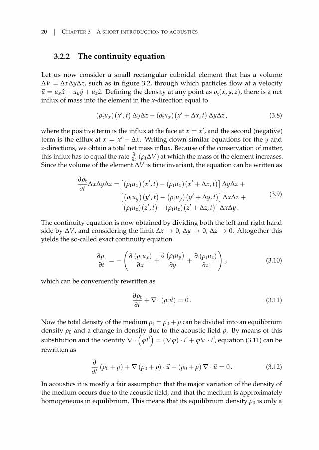
3.2.2 The continuity equation
Let us now consider a small rectangular cuboidal element that has a volume∆V = ∆x∆y∆z, such as in figure 3.2, through which particles flow at a velocity~u = ux x + uyy + uz z. Defining the density at any point as ρt(x, y, z), there is a netinflux of mass into the element in the x-direction equal to
(ρtux)(
x′, t)
∆y∆z− (ρtux)(x′ + ∆x, t
)∆y∆z , (3.8)
where the positive term is the influx at the face at x = x′, and the second (negative)term is the efflux at x = x′ + ∆x. Writing down similar equations for the y andz-directions, we obtain a total net mass influx. Because of the conservation of matter,this influx has to equal the rate ∂
∂t (ρt∆V) at which the mass of the element increases.Since the volume of the element ∆V is time invariant, the equation can be written as
∂ρt
∂t∆x∆y∆z =
[(ρtux)
(x′, t
)− (ρtux)
(x′ + ∆x, t
)]∆y∆z +[(
ρtuy)(
y′, t)−(ρtuy
)(y′ + ∆y, t
)]∆x∆z +[
(ρtuz)(z′, t)− (ρtuz)
(z′ + ∆z, t
)]∆x∆y .
(3.9)
The continuity equation is now obtained by dividing both the left and right handside by ∆V, and considering the limit ∆x → 0, ∆y → 0, ∆z → 0. Altogether thisyields the so-called exact continuity equation
∂ρt
∂t= −
(∂ (ρtux)
∂x+
∂(ρtuy
)∂y
+∂ (ρtuz)
∂z
), (3.10)
which can be conveniently rewritten as
∂ρt
∂t+∇ · (ρt~u) = 0 . (3.11)
Now the total density of the medium ρt = ρ0 + ρ can be divided into an equilibriumdensity ρ0 and a change in density due to the acoustic field ρ. By means of thissubstitution and the identity ∇ ·
(ϕ~F)= (∇ϕ) · ~F + ϕ∇ · ~F, equation (3.11) can be
rewritten as
∂
∂t(ρ0 + ρ) +∇ (ρ0 + ρ) · ~u + (ρ0 + ρ)∇ · ~u = 0 . (3.12)
In acoustics it is mostly a fair assumption that the major variation of the density ofthe medium occurs due to the acoustic field, and that the medium is approximatelyhomogeneous in equilibrium. This means that its equilibrium density ρ0 is only a
3.2 PARTICLES, PRESSURE AND SOUND VELOCITY 21
x
yz
∆x
∆y
∆z
(ρtux)(x′, t) (ρtux)(x′ + ∆x, t)
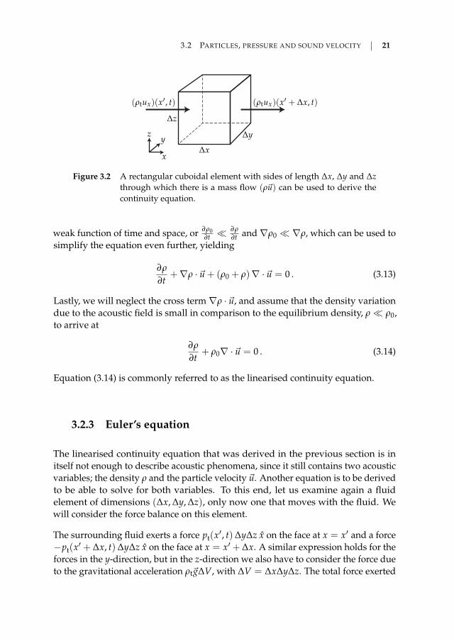
Figure 3.2 A rectangular cuboidal element with sides of length ∆x, ∆y and ∆zthrough which there is a mass flow (ρ~u) can be used to derive thecontinuity equation.
weak function of time and space, or ∂ρ0∂t
∂ρ∂t and∇ρ0 ∇ρ, which can be used to
simplify the equation even further, yielding
∂ρ
∂t+∇ρ · ~u + (ρ0 + ρ)∇ · ~u = 0 . (3.13)
Lastly, we will neglect the cross term ∇ρ · ~u, and assume that the density variationdue to the acoustic field is small in comparison to the equilibrium density, ρ ρ0,to arrive at
∂ρ
∂t+ ρ0∇ · ~u = 0 . (3.14)
Equation (3.14) is commonly referred to as the linearised continuity equation.
3.2.3 Euler’s equation
The linearised continuity equation that was derived in the previous section is initself not enough to describe acoustic phenomena, since it still contains two acousticvariables; the density ρ and the particle velocity ~u. Another equation is to be derivedto be able to solve for both variables. To this end, let us examine again a fluidelement of dimensions (∆x, ∆y, ∆z), only now one that moves with the fluid. Wewill consider the force balance on this element.
The surrounding fluid exerts a force pt(x′, t)∆y∆z x on the face at x = x′ and a force−pt(x′ + ∆x, t)∆y∆z x on the face at x = x′ + ∆x. A similar expression holds for theforces in the y-direction, but in the z-direction we also have to consider the force dueto the gravitational acceleration ρt~g∆V, with ∆V = ∆x∆y∆z. The total force exerted
22 CHAPTER 3 A SHORT INTRODUCTION TO ACOUSTICS
on the volume element in all directions is therefore
~F(x, y, z, t) =
(pt(x′, t)− pt(x′ + ∆x, t)
∆xx +
pt(y′, t)− pt(y
′ + ∆y, t)∆y
y +
pt(z′, t)− pt(z
′ + ∆z, t)∆z
z + ρt~g
)∆V .
(3.15)
This force causes an acceleration of the fluid element equal to~a = d~u/dt, which canbe expanded through application of the chain rule
~a =∂~u∂t
+ ux∂~u∂x
+ uy∂~u∂y
+ uz∂~u∂z
=∂~u∂t
+ (~u · ∇) u .(3.16)
Equations (3.15) and (3.16) can be combined by means of Newton’s second law~F = ρt∆V~a. Moreover looking at the limit ∆x → 0, ∆y→ 0, ∆z→ 0, one obtains
−∇pt + ρt~g = ρt
(∂~u∂t
+ (~u · ∇)~u)
. (3.17)
In equilibrium we have that −∇p0 +~gρ0 = 0, which means that ∇pt = ∇p +~gρ0,and therefore
−∇p + ρ~g = (ρ0 + ρ)
(∂~u∂t
+ (~u · ∇)~u)
. (3.18)
Let us now assume that |ρ~g| |∇p|, |ρ| ρ0 and |(~u · ∇)~u| ∣∣∣ ∂~u
∂t
∣∣∣. This yieldsthe linear Euler’s equation:
∇p + ρ0∂~u∂t
= 0 . (3.19)
3.2.4 The wave equation
The linearised continuity equation and the linear form of Euler’s equation can becombined to arrive at a single equation describing sound waves of small amp-litudes. Taking the time derivative of (3.14) and the divergence of (3.19) results in
3.3 SIMPLE TYPES OF SOUND WAVES 23
the equations
∂2ρ
∂t2 +∇ ·(
ρ0∂~u∂t
)= 0 (3.20a)
∇2 p +∇ ·(
ρ0∂~u∂t
)= 0 (3.20b)
in which ∇2 = ∇ · ∇ is the Laplacian. Combination of both equations yields
∇2 p− ∂2ρ
∂t2 = 0 , (3.21)
which can be simplified even further making use of the equation of state (3.5) toarrive at the linearised lossless wave equation for propagation in fluids:
∇2 p− 1c2
∂2 p∂t2 = 0 , (3.22)
Assuming that all quantities vary at a single radial frequency ω, and thus p = Aejωt,(3.22) can be written as the Helmholtz equation
∇2 p + k2 p = 0 , (3.23)
where k = ω/c is the angular wave number.
3.3 Simple types of sound waves
In this section, two simple types of sound waves are considered; the plane wave andthe spherical sound wave. Their simplicity is due to their one-dimensional nature intheir respective coordinate systems (Cartesian or spherical).
3.3.1 Plane waves
Plane waves, such as shown in figure 3.1, are sound waves of which the pressureand particle velocity only depend on a single coordinate in a Cartesian coordinatesystem. Let us choose the z-axis for this purpose. This reduces equation (3.22) to asomewhat simpler form:
∂2 p∂z2 −
1c2
∂2 p∂t2 = 0 . (3.24)

24 CHAPTER 3 A SHORT INTRODUCTION TO ACOUSTICS
It can be shown (see for example [69]) that solutions of this equation are of theform p(z, t) = f (z− ct) and p(z, t) = g(z + ct). These are waves that propagate inunaltered shape and amplitude in the positive and negative z-direction respectively,with a velocity c. Thus the constant c that was introduced in equation (3.5) turns outto be the sound velocity. The particle velocity in the wave can be found by meansof equation (3.19), which can be written for a plane wave that propagates in thez-direction as
∂ p∂z
+ ρ0∂uz
∂t= 0 . (3.25)
This equation can be rewritten making use of the substitution s = z− ct.
∂ p∂s
∂s∂z
+ ρ0∂uz
∂s∂s∂t
= 0
∂ p∂s− ρ0c
∂uz
∂s= 0
(3.26)
Integration of the above equation with regard to s yields the relationship betweenthe excess pressure and the particle velocity; uz =
1ρ0c p. Likewise the substitution
s = z + ct results in uz = − 1ρ0c p, which is consistent with the definition of a
backwards travelling wave. The quantity
Za0 =
puz
(3.27)
is the specific, or characteristic acoustic impedance of the medium, which, for aplane wave, is equal to Za
0 = ρ0c.
3.3.2 Spherical waves
In the case of a spherical wave the only variation occurs as a function of the radialdistance from the sound source r and time t. The pressure and particle velocities donot vary in the θ and ϕ directions. Analogously to the previous section, the waveequation (3.22) can be rewritten for this specific case making use of the identitiesx = r sin θ cos ϕ, y = r sin θ sin ϕ and z = r cos θ, obtaining
∂2 p∂r2 +
2r
∂ p∂r− 1
c2∂2 p∂t2 = 0 , (3.28)
Substitution of p(r, t) = 1r f (r, t) results in
∂2 f∂r2 −
1c2
∂2 f∂t2 = 0 (3.29)
3.3 SIMPLE TYPES OF SOUND WAVES 25
which is again in the same form as the one dimensional wave equation (3.24). Thesolution of the differential equation is therefore found in the same manner. Weobtain for the pressure distribution p(r, t) = 1
r f (r− ct), which corresponds to aradially expanding wave. The solution p(r, t) = 1
r g(r + ct) exists as well of course,but describes a radially contracting wave (a wave propagating radially towardsr = 0), which is less interesting to consider.
Making use again of (3.19) and (B.4) in appendix B (page 174), we have that
∂ p∂r
+ ρ0∂ur
∂t= 0 . (3.30)
Let us now assume that the pressure varies sinusoidally. For matters of simplicity,we will write it in complex notation as
p(r, t) =1r
A ej(ωt−kr) , (3.31)
with the angular wave number k = ω/c. This reduces equation (3.30) to
ur =1
ρ0c
(1 +
1jkr
)p(r, t) . (3.32)
The specific impedance for a spherically expanding wave is found from the previousequation:
Za0 = ρ0c
11 + 1
jkr
=ρ0c
1 + k2r2
(k2r2 + jkr
).
(3.33)
Contrarily to the plane wave, in which the pressure and the particle velocity areexactly in phase, the phase difference between both variables varies with the distancefrom the origin in a spherical wave. The factor kr can be written as kr = 2πr/λ,making the specific impedance depend on the ratio between the distance from theorigin and the wavelength. The pressure and particle velocity are exactly out ofphase for r/λ = 0, while for r/λ→ ∞ they are in phase, and the specific impedanceseen by the wave is again the same as in the plane wave case:
Za0
∣∣∣r→∞
= ρ0c . (3.34)

26 CHAPTER 3 A SHORT INTRODUCTION TO ACOUSTICS
The point source
If a spherical source pulsates with a velocity U0ejωt and has a radius a, we can findfrom 3.33 that the pressure at the surface of the source is
p(a, t) = u(a, t) Za0(a) ,
=1
1 + 1jka
ρ0cU0ejωt ,(3.35)
Combination of the latter with equation (3.31) yields
p(r, t) = ρ0cU0jka
1 + jkaar
ej(ωt+k(a−r)) , (3.36)
which in case of a long wavelength in comparison to the source radius reduces to
p(r, t) = jρ0cU0ka2
rej(ωt−kr) , ka 1 . (3.37)
The volume velocity Q that is produced by our spherical source is equal to its velocitymultiplied by its surface area. Consequently the volume velocity amplitude is
Q0 = 4πa2U0 . (3.38)
which allows the expression for the sound pressure to be simplified to
p(r, t) =jωρ0Q0
4πrej(ωt−kr) . (3.39)
Combination with (3.32) finally yields an expression of the particle velocity that isproduced by this source:
~u(r, t) =Q0
4πr2 (1 + jkr) ej(ωt−kr) r . (3.40)
As mentioned, these expressions are only valid for long wavelengths in comparisonto the radius of the spherical source. In the case of a point source, having aninfinitesimally small radius, however, these equations are exact, as long as thefrequency, and therefore k, is finite.
3.4 Attenuation of sound
Until now the influence of attenuation of sound waves was neglected in the dis-cussion of wave propagation. While in many cases this is a fair assumption, the

3.5 POWER AND SOUND INTENSITY 27
theory put forward here will be used to discuss energy transfer by means of soundwaves. This means that it is imperative to, at the very least, consider attenuation,and to investigate whether or not it can be neglected. This section slightly extendsthe theory described above to allow it to describe the effect that absorption has onthe sound wave.
It would go too far for this short introduction to acoustics to discuss the theory ofattenuation in gases and fluids and to derive sound wave equations that reflect theseeffects. Instead the result will be merely given here. More details can be found instandard works on acoustics. For example [58] contains an excellent analysis ofabsorption and attenuation. As Kinsler et al. describe, there are multiple effects atplay that result in attenuation of a sound wave. Generally they all lead to a lossyHelmholtz equation
∇2 p + k2
p = 0 . (3.41)
This equation is very similar to the Helmholtz equation (3.23) that was derivedearlier. The only difference is the substitution of a complex valued angular wavenumber
k = k− jα . (3.42)
Here k is still defined as the ratio of the angular frequency to the sound velocity,i.e. k = ω/c. Attenuation of sound waves is accounted for by introduction ofthe absorption coefficient α of the medium, which is a function, not only of theparameters of the medium, such as its chemical composition, temperature andpressure, but also of the frequency of the sound propagating through it.
3.5 Power and sound intensity
As the particles in a sound wave have a certain mass, their vibration implies thatthey possess a certain amount of kinetic energy. Likewise, the pressure variationsin the gas require the exchange of potential energy within the sound wave. Thepresence of these forms of energy in a sound wave is of course the very reason thatsound can be used to transfer energy.
3.5.1 Sound intensity
The energy that is transferred by a sound wave through a certain area perpendicularto the direction of propagation of the wave, is equal to the work performed by the
28 CHAPTER 3 A SHORT INTRODUCTION TO ACOUSTICS
particles adjacent to this area [35]. The rate of work that is done is equal to theproduct of the force ~F that is exerted on and the velocity ~u of the particles. The rateof work per unit area is then given by
ddS
dWdt
= pun (3.43)
in which dS is an infinitesimally small area and un the component of the particlevelocity normal to the surface. Generalising this concept we can define a vectorquantity
~I(t) = p(t)~u(t) , (3.44)
which is the instantaneous sound intensity. It is in essence the energy flux density ofthe sound wave, i.e. the amount of energy that passes per unit time through a unitarea.
In a time-stationary acoustic field, the instantaneous sound intensity can be split upinto an active and a reactive component [35]. The active sound intensity ~Ia is thetime average of the instantaneous sound intensity
~Ia =1T
t0+T∫t0
p(t)~u(t)dt , (3.45)
and as such represents the net transport of energy in the direction of ~Ia. The in-tegration length T in this equation is chosen so that averaging takes place over aninteger number of periods of the sound wave. Note that although the active soundintensity no longer contains a time dependency, it is a vector which still dependson the spatial position in the sound field. The reactive part of the sound intensityrepresents the locally oscillating exchange of energy in the sound field, withoutactual transport or dissipation.
The term ‘sound intensity’ is often interpreted as the average flow of energy in thedirection of propagation ‖~Ia‖, which is of course only meaningful when the soundwave has a distinct direction of propagation, such as a plane wave. If the vector~Ia isa function of spatial coordinates as well one can still talk about the the magnitudeof the sound intensity Ia = ‖~Ia‖, but this has a different meaning in most cases, asit is the active sound intensity in the local direction of propagation (which is ~u/‖~u‖).Whenever the scalar Ia is used in this thesis, it will have the latter meaning to avoidconfusion. Whenever one can speak of one single direction of propagation of thesound wave, Ia will be the active sound intensity of the wave. In all other cases thevector intensity~I will be used.
In acoustics mostly periodic signals with a zero average are considered, whichrenders the concept of intensity somewhat easier. In this case both the pressure and
3.5 POWER AND SOUND INTENSITY 29
particle velocity can be written as a linear combination of sinusoids at frequenciesthat are an integer multiple of a fundamental frequency ω. The pressure field canthen be written as
p(~r, t) =∞
∑m=1
Pm(~r) cos(mωt + ϕp,m
). (3.46)
An analogous expression can be found for the particle velocity
~u(~r, t) =∞
∑n=1
Un(~r) cos(nωt + ϕu,n) u . (3.47)
The instantaneous sound intensity is subsequently found by combining the previoustwo equations and (3.44), yielding
~I(~r, t) =∞
∑m=1
[Pm(~r) cos
(mωt + ϕp,m
)] ∞
∑n=1
[~Un(~r) cos(nωt + ϕu,n)
]=
∞
∑m=1
∞
∑n=1
~Im,n(~r, t)(3.48)
The product~Im,n of the m-th term of the pressure and the n-th term of the particlevelocity is
~Im,n(~r, t) = Pm(~r) cos(mωt + ϕp,m
)~Un(~r) cos(nωt + ϕu,n)
= 12 Pm(~r) ~Un(~r)
[cos((m + n)ωt +
(ϕp,m + ϕu,n
))+
cos((m− n)ωt +
(ϕp,m − ϕu,n
)) ] (3.49)
It is clear from equations (3.45), (3.48) and (3.49) that the only components thatcontribute to the active sound intensity, and hence to the net transport of energy, arethose components that are of equal frequency (m = n) and have a phase differenceunequal to 1
2 π (i.e. ϕp,m − ϕu,n 6= 12 π (mod π))
To simplify matters even further, let us suppose that we have a pressure field thatvaries purely sinusoidally, i.e. p(~r, t) = P(~r) cos
(ωt + ϕp
), and a particle velocity
~u(~r, t) = ~U(~r) cos(ωt + ϕu). There are no higher harmonics present, contrarily tothe previous discussion. From the results above we have that
~Ia(~r, t0) =P(~r) ~U(~r)
2T
t0+2πω∫
t0
[cos(2ωt +
(ϕp + ϕu
))+ cos
(ϕp − ϕu
)]dt
= 12 P(~r) ~U(~r) cos
(ϕp − ϕu
).
(3.50)
30 CHAPTER 3 A SHORT INTRODUCTION TO ACOUSTICS
When the excess sound pressure and the particle velocity are written in complex
notation p(~r, t) = P(~r) ej(ωt+ϕp) and~u(~r, t) = ~U(~r) ej(ωt+ϕu), one can show that theactive sound intensity is
~Ia(~r) =12 Re
(p(~r, t)~u
∗(~r, t)
). (3.51)
3.6 Equivalent electrical networks
Any system of linear time-invariant differential equations can be represented byan equivalent electrical network. Such networks can prove enormously insightful,especially for electrical engineers who are used to working with such diagrams. Thepurpose of an electrical network is to capture the (most important) behaviour of asystem in a diagram. The use of these circuits, however, is not only limited to elec-trical problems. Any problem that can be described by (linear) differential equationscan be captured into such an equivalent network. Ideal capacitors and inductors,having the voltage-current relationships v = L di
dt and i = C dvdt respectively, are then
used to represent differentiation and integration.
The cornerstone of electrical networks is the concept of impedance, introduced byOliver Heaviside, which is defined as the ratio of the voltage across an element tothe current through it. As already discussed in section 1.2, this thesis uses
Za=
pu
(3.52)
as definition for the acoustic impedance. The superscript a is used to indicatean acoustic impedance. From this definition we find that pressure is equival-ent to a voltage and particle velocity to a current. Furthermore, the relationshipp = Za u = jωm u shows that an inductance is equivalent to an inertance per unitarea m on which the pressure p acts. A mechanical equivalent would be a massper unit area. Equivalently, an acoustic compliance per unit area n, which behavesaccording to n d p
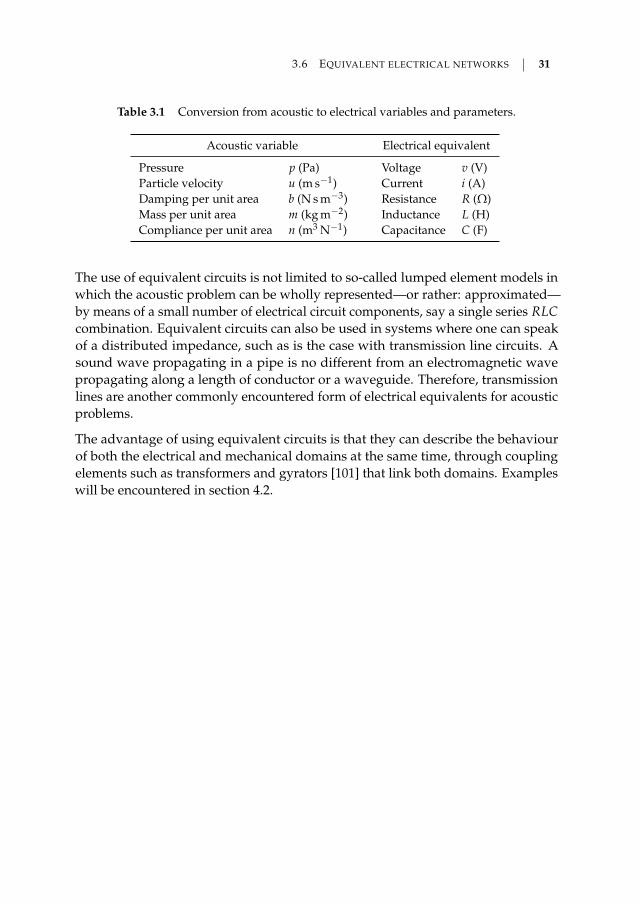
dt = u, translates to capacitance in the electrical case. These relation-ships are summarised in table 3.1.
In principle, the use of equivalent circuits is restricted to one-dimensional acousticproblems, since the current in such a diagram is a scalar quantity. As such, it cannotbe used to describe a general particle velocity, which is a vector. Therefore, thedirection of ~u should be implicitly defined, as is the case in a one-dimensional wave,such as the plane wave or the spherical wave that were discussed earlier in sections3.3.1 and 3.3.2.
3.6 EQUIVALENT ELECTRICAL NETWORKS 31
Table 3.1 Conversion from acoustic to electrical variables and parameters.
Acoustic variable Electrical equivalent
Pressure p (Pa) Voltage v (V)Particle velocity u (m s−1) Current i (A)Damping per unit area b (N s m−3) Resistance R (Ω)Mass per unit area m (kg m−2) Inductance L (H)Compliance per unit area n (m3 N−1) Capacitance C (F)
The use of equivalent circuits is not limited to so-called lumped element models inwhich the acoustic problem can be wholly represented—or rather: approximated—by means of a small number of electrical circuit components, say a single series RLCcombination. Equivalent circuits can also be used in systems where one can speakof a distributed impedance, such as is the case with transmission line circuits. Asound wave propagating in a pipe is no different from an electromagnetic wavepropagating along a length of conductor or a waveguide. Therefore, transmissionlines are another commonly encountered form of electrical equivalents for acousticproblems.
The advantage of using equivalent circuits is that they can describe the behaviourof both the electrical and mechanical domains at the same time, through couplingelements such as transformers and gyrators [101] that link both domains. Exampleswill be encountered in section 4.2.

CH
AP
TE
R
4 First steps in acousticenergy transfer
THERE are two main performance indices for any system that is used to transferenergy, independently of whether or not it achieves it contactlessly. These arethe energy transfer efficiency on one hand, and the power transfer capabilities
on the other. These two factors determine the physical limitations of such a system.One expects a part of a system that transfers energy to do so without impeding theenergy flow, and thus without posing any restriction on the power flow through it,within the limits in which the system is to be used of course. Efficiency is always akey aspect, as it determines how economically sound an energy transfer system is,and how much heating is to be expected. It is often the most interesting aspect onthe basis of which to compare energy transfer systems.
Of course there are other characteristics of contactless energy transfer systems thatcan be of importance when trying to determine the best candidate in any situation,but these can be rather application dependent. One can think of issues such as thestrength or presence of electromagnetic fields, for example with regard to safety,or whether there are obstacles in the line of sight between the transmitter and thereceiver, the medium through which the energy is to be transmitted (especiallymetallic barriers can pose great difficulties for methods that rely on electromagneticfields) or limitations on system dimensions, just to name a few.
The purpose of this chapter is to take a first look at the energy transfer that canbe attained by means of contactless energy transfer through air. Therefore we will
This chapter is based on [98] and [100].
33

34 CHAPTER 4 FIRST STEPS IN ACOUSTIC ENERGY TRANSFER
have to look at the specific loss mechanisms that occur in such an application.When talking specifically about acoustic energy transfer systems, the energy transferefficiency is limited chiefly by four effects:
• the attenuation of sound waves in the medium;
• the spreading of the sound waves;
• the transduction efficiency;
• losses in electrical circuitry.
Modelling these effects is necessary to be able to judge the attainable efficiency.
Attenuation Attenuation of sound waves in a medium occurs through a num-ber of different principles, which vary according to the type of medium and caninclude viscous or frictional losses, heat conduction, molecular thermal relaxation,structural relaxation, chemical relaxation, losses at boundaries, crystal lattice defects,scattering in polycrystalline materials, and so forth [58, 69].
Spreading Parts of the sound wave that do not reach the receiver surface willpropagate into infinity and will be absorbed at some point. As such they do not con-tribute to the output power at the receiving end. Therefore these can be consideredas losses, which can be grouped under spreading losses. Spreading of sound wavescan occur naturally because of the radiation pattern of the source. In practice virtu-ally no sound source radiates a collimated beam, but will always create a divergentradiation pattern. Spreading can also occur because of a change in the directionof propagation of the sound wave, because of either refraction or diffraction [85].Refraction is the bending of sound waves due to a change in the medium. Onecan think of a change in sound velocity due to local temperature variation of themedium, for example. Diffraction is the bending of sound waves around objects.
Transduction The transduction efficiency takes into account the losses that oc-cur in the transducer which converts the electrical energy into mechanical vibrationsat the transmitting side and vice versa at the receiving end. Any losses in thisprocess, whether they be of electrical or mechanical origin, will decrease the amountof energy that is transferred to an application that is to be powered.
Circuitry In order to work, an acoustic energy transfer system requires electricalcircuitry at the transmitting and receiving ends, which inherently introduce losses.These losses fall outside the scope of this thesis, as they are a field of research inthemselves, depending on the circuit topologies that are chosen.
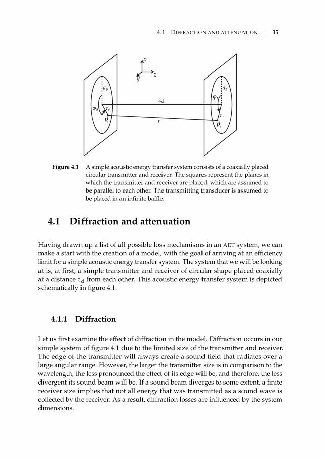
4.1 DIFFRACTION AND ATTENUATION 35
as ar
ϕs
ϕrzd
r
x
y z
rsrrPs Pr
Figure 4.1 A simple acoustic energy transfer system consists of a coaxially placedcircular transmitter and receiver. The squares represent the planes inwhich the transmitter and receiver are placed, which are assumed tobe parallel to each other. The transmitting transducer is assumed tobe placed in an infinite baffle.
4.1 Diffraction and attenuation
Having drawn up a list of all possible loss mechanisms in an AET system, we canmake a start with the creation of a model, with the goal of arriving at an efficiencylimit for a simple acoustic energy transfer system. The system that we will be lookingat is, at first, a simple transmitter and receiver of circular shape placed coaxiallyat a distance zd from each other. This acoustic energy transfer system is depictedschematically in figure 4.1.
4.1.1 Diffraction
Let us first examine the effect of diffraction in the model. Diffraction occurs in oursimple system of figure 4.1 due to the limited size of the transmitter and receiver.The edge of the transmitter will always create a sound field that radiates over alarge angular range. However, the larger the transmitter size is in comparison to thewavelength, the less pronounced the effect of its edge will be, and therefore, the lessdivergent its sound beam will be. If a sound beam diverges to some extent, a finitereceiver size implies that not all energy that was transmitted as a sound wave iscollected by the receiver. As a result, diffraction losses are influenced by the systemdimensions.

36 CHAPTER 4 FIRST STEPS IN ACOUSTIC ENERGY TRANSFER
Some further assumptions about the system will have to be made, if we are to beable to calculate the influence of the spreading for the simple AET system describedabove. Here we will make the assumption that the front face of the transmittingtransducer vibrates as a whole, without flexing or bending at any point. This typeof source can be modelled as a classical source: what is known in literature as avibrating piston source [21, 58, 69, 85, 120]. This is essentially a circular disk of radiusas which is mounted in an infinite baffle, of which the surface uniformly performssinusoidal vibrations with a velocity amplitude U0 and angular frequency ω.
Pressure and particle velocity
It is possible to calculate the pressure and particle velocity that are generated by sucha piston by considering its surface to be made up of an infinite number of individualbaffled point sources. The superposition of the pressure field of each individualpoint source results in the total pressure field of the piston source, which is achievedby integration over the piston surface. This method is commonly referred to as aRayleigh integral, and is a special case of the more general Kirchhoff diffractionformula [69, 82].
The piston vibrates with a velocity u = U0ejωt, which means that every point of thepiston moves at this same velocity. Every infinitesimally small section of the pistonsurface of area dS therefore produces a volume velocity dQ = udS. Consequently,the volume velocity amplitude is dQ0 = U0dS. The pressure that is generated bysuch a single point source at a distance r is found with help from equation (3.39) tobe
dpp =jωρ0U0
2πrej(ωt−kr)dS . (4.1)
The corresponding particle velocity that is produced by this point source is analog-ously found from (3.40) to be
d~up =U0
2πr2
(1 + jkr
)ej(ωt−kr) rpdS . (4.2)
These equations contain a complex angular wave number k = k− jα to account forthe absorption by the medium by means of an absorption coefficient, as explainedin section 3.4. The distance r between each source point ~Ps = rsr + ϕs ϕ and receiverpoint ~Pr = rrr + ϕr ϕ + zdz is given by
r =∥∥∥~Ps − ~Pr
∥∥∥=√
r2s + r2
r + z2d − 2rsrr cos(ϕs − ϕr) .
(4.3)
4.1 DIFFRACTION AND ATTENUATION 37
The unit vector rp points in the radial direction away from the source point. Thedirection of d~up at the receiver point ~Pr is therefore the direction of the line ~Ps~Pr. Thisunit vector can be written in terms of the unit vectors in the Cartesian coordinatesystem in figure 4.1, as
rp =1r
((rr cos ϕr − rs cos ϕs) x + (rr sin ϕr − rs sin ϕs) y + zdz
)(4.4)
Without loss of generality, the case ϕr = 0 can be considered, since the problem issymmetric around the z-axis. The total sound pressure and particle velocity at anypoint in the field can then be found by integration over the surface of the transmitter.Denoting the area of the transmitter by As, the pressure is found from (4.1) to be
p(rr, zd, t) =∫∫As
dpp
=jωρ0U0
2πejωt
as∫0
2π∫0
e−jkr
rrsdϕsdrs .
(4.5)
The particle velocity is found in exactly the same manner by integration of d~up from(4.2). It is equal to
~u(rr, zd, t) =∫∫As
d~up
=U0
2πejωt
as∫0
2π∫0
e−jkr
r2
(1 + jkr
)×
1r((rr − rs cos ϕs) x− rs sin ϕsy + zdz) rsdϕsdrs .
(4.6)
Here as is the radius of the transmitter, and zd is the distance between the transmitterand the receiver.
Careful examination of the system reveals that for ϕr = 0 there is no net contributionof the y-component of the integrand in the calculation of the particle velocity inequation (4.6) due to rotational symmetry. Therefore the y-component of~u is equal tozero. The calculated x-component of the particle velocity is equal to the r-componentin the cylindrical coordinate system. Moreover, the inner integral in both (4.5) and(4.6) can be rewritten employing the system’s symmetry, since in both integrals thecontributions of the intervals [0; π] and [π; 2π] are equal. Hence the equations for
38 CHAPTER 4 FIRST STEPS IN ACOUSTIC ENERGY TRANSFER
the pressure and particle velocity produced by the vibrating piston reduce to
p(rr, zd, t) = jωρ0U0
πejωt
as∫0
π∫0
e−jkr
rrsdϕsdrs
~u(rr, zd, t) =U0
πejωt
as∫0
π∫0
e−jkr
r2
(1 + jkr
)×
1r((rr − rs cos ϕs) r + zdz) rsdϕsdrs .
(4.7)
From pressure to power
As was explained in section 3.5.1, the energy flux density of a (sound) pressure waveis characterised by the associated sound intensity. The sound intensity vector atany point in space in a homogenous gaseous medium can be calculated from theexpressions for the pressure and particle velocity in (4.7) using (3.51):
~Ia(rr, zd) =12 Re
(p~u∗)
= Ia,r r + Ia,z z ,(4.8)
The total intensity at any point is then found from the euclidian norm of the intensityvector:
Ia(rr, zd) =∥∥∥~Ia
∥∥∥=√
I2a,r + I2
a,z .(4.9)
Numeric integration, e.g. by means of the MATLAB integral2 function, allows thecalculation of the diffraction pattern of the circular piston source. An example ofsuch a pattern is shown in figure 4.2 as a function of z and r. Attenuation wasomitted in this simulation, i.e. k = k.
As is immediately clear from the radiation pattern, the diffraction that occurs at theedge of the piston itself prevents a truly perfect focus. A piston source does notproduce a plane wave, but it rather creates a main on-axis lobe and many so-calledside lobes. Both the main and the side lobes diverge, and therefore a receiver offinite dimensions will never be able to collect all radiated energy.
Figure 4.2 shows a clear focal point to the radiation pattern of the source wherethe sound intensity is the greatest, around zd = 400 mm. This focal point can beemployed for AET, although placement of the receiver at this location does not
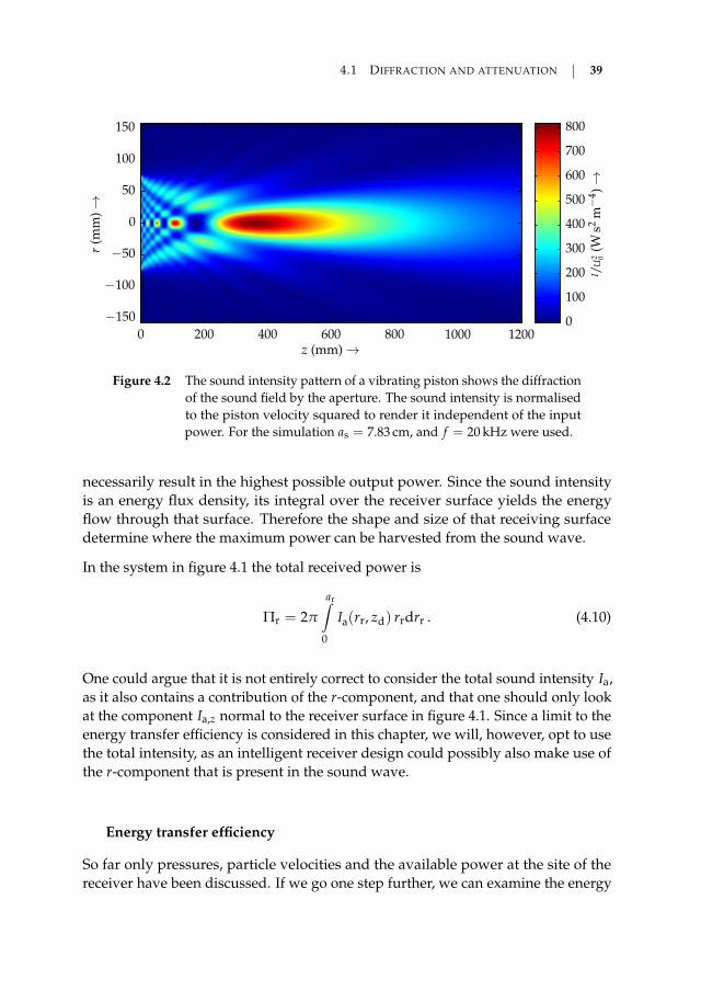
4.1 DIFFRACTION AND ATTENUATION 39
I /U
2 0(W
s2m
−4)→
r(m
m)→
z (mm) →
0 200 400 600 800 1000 12000
100
200
300
400
500
600
700
800
−150
−100
−50
0
50
100
150
Figure 4.2 The sound intensity pattern of a vibrating piston shows the diffractionof the sound field by the aperture. The sound intensity is normalisedto the piston velocity squared to render it independent of the inputpower. For the simulation as = 7.83 cm, and f = 20 kHz were used.
necessarily result in the highest possible output power. Since the sound intensityis an energy flux density, its integral over the receiver surface yields the energyflow through that surface. Therefore the shape and size of that receiving surfacedetermine where the maximum power can be harvested from the sound wave.
In the system in figure 4.1 the total received power is
Πr = 2π
ar∫0
Ia(rr, zd) rrdrr . (4.10)
One could argue that it is not entirely correct to consider the total sound intensity Ia,as it also contains a contribution of the r-component, and that one should only lookat the component Ia,z normal to the receiver surface in figure 4.1. Since a limit to theenergy transfer efficiency is considered in this chapter, we will, however, opt to usethe total intensity, as an intelligent receiver design could possibly also make use ofthe r-component that is present in the sound wave.
Energy transfer efficiency
So far only pressures, particle velocities and the available power at the site of thereceiver have been discussed. If we go one step further, we can examine the energy

40 CHAPTER 4 FIRST STEPS IN ACOUSTIC ENERGY TRANSFER
Xrad
πa2s Za
0
Rrad
πa2s Za
0Z
rad
πa
2 sZ
a 0
(−)→
kas (−) →10−1 100 101 1020
0.2
0.4
0.6
0.8
1
1.2
1.4
Figure 4.3 The normalised radiation impedance of a circular piston source con-verges to Zrad
/πa2
s Za0 = 1 + j0 for high values of kas.
transfer efficiency due to diffraction ηdif, which can be defined as the ratio of thereceived power to the total radiated power
ηdif =Πr
Πrad. (4.11)
Without going into detail, the radiation impedance, i.e. the ratio of force over velocity,that the piston works against is given by (see for example [58, 69])
Zrad = Rrad + jXrad
= ρ0cπa2s
(1− 2
J1(2kas)
2kas+ j2
H1(2kas)
2kas
),
(4.12)
with J1(x) the first-order Bessel function of the first kind and H1(x) the first orderStruve function [3, 5]. For completeness, the radiation impedance is plotted in figure4.3 as a function of kas.
The power that is radiated by the source is then found from
Πrad = 12 U2
0 Rrad
= 12 U2
0 ρ0cπa2s
(1− 2
J1(2kas)
2kas
),
(4.13)
Combining equations (4.10), (4.11) and (4.13), the diffraction dependent ratio of
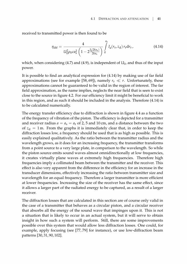
4.1 DIFFRACTION AND ATTENUATION 41
received to transmitted power is then found to be
ηdif =4
U20 ρ0ca2
s
(1− 2 J1(2kas)
2kas
) ar∫0
Ia(rr, zd) rrdrr , (4.14)
which, when considering (4.7) and (4.9), is independent of U0, and thus of the inputpower.
It is possible to find an analytical expression for (4.14) by making use of far fieldapproximations (see for example [58, 69]), namely rr r. Unfortunately, theseapproximations cannot be guaranteed to be valid in the region of interest. The farfield approximation, as the name implies, neglects the near field that is seen to existclose to the source in figure 4.2. For our efficiency limit it might be beneficial to workin this region, and as such it should be included in the analysis. Therefore (4.14) isto be calculated numerically.
The energy transfer efficiency due to diffraction is shown in figure 4.4 as a functionof the frequency of vibration of the piston. The efficiency is depicted for a transmitterand receiver radius a = as = ar of 2, 5 and 10 cm, and a distance between the twoof zd = 1 m. From the graphs it is immediately clear that, in order to keep thediffraction losses low, a frequency should be used that is as high as possible. This iseasily explained qualitatively. As the ratio between the transmitter radius and thewavelength grows, as it does for an increasing frequency, the transmitter transformsfrom a point source to a very large plate, in comparison to the wavelength. So whilethe piston source emits sound waves almost omnidirectionally at low frequencies,it creates virtually plane waves at extremely high frequencies. Therefore highfrequencies imply a collimated beam between the transmitter and the receiver. Thiseffect is also very apparent from the difference in the efficiency for an increase in thetransducer dimensions, effectively increasing the ratio between transmitter size andwavelength for an equal frequency. Therefore a larger transmitter is more efficientat lower frequencies. Increasing the size of the receiver has the same effect, sinceit allows a larger part of the radiated energy to be captured, as a result of a largerreceiver.
The diffraction losses that are calculated in this section are of course only valid inthe case of a transmitter that behaves as a circular piston, and a circular receiverthat absorbs all the energy of the sound wave that impinges upon it. This is nota situation that is likely to occur in an actual system, but it will serve to obtaininsight in how such a system will perform. Still, there are some improvementspossible over this system that would allow less diffraction losses. One could, forexample, apply focusing (see [77, 79] for instance), or use low-diffraction beampatterns [30, 31, 90, 102].
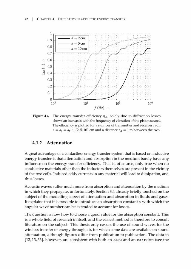
42 CHAPTER 4 FIRST STEPS IN ACOUSTIC ENERGY TRANSFER
a = 10 cm
a = 5 cm
a = 2 cm
ηd
if(−
)→
f (Hz) →103 104 105 1060
0.1
0.2
0.3
0.4
0.5
0.6
0.7
0.8
0.9
1
Figure 4.4 The energy transfer efficiency ηdif solely due to diffraction lossesshows an increases with the frequency of vibration of the piston source.The efficiency is plotted for a number of transmitter and receiver radiia = as = ar ∈ 2, 5, 10 cm and a distance zd = 1 m between the two.
4.1.2 Attenuation
A great advantage of a contactless energy transfer system that is based on inductiveenergy transfer is that attenuation and absorption in the medium barely have anyinfluence on the energy transfer efficiency. This is, of course, only true when noconductive materials other than the inductors themselves are present in the vicinityof the two coils. Induced eddy currents in any material will lead to dissipation, andthus losses.
Acoustic waves suffer much more from absorption and attenuation by the mediumin which they propagate, unfortunately. Section 3.4 already briefly touched on thesubject of the modelling aspect of attenuation and absorption in fluids and gases.It explains that it is possible to introduce an absorption constant α with which theangular wave number can be extended to account for losses.
The question is now how to choose a good value for the absorption constant. Thisis a whole field of research in itself, and the easiest method is therefore to consultliterature on the subject. This thesis only covers the use of sound waves for thewireless transfer of energy through air, for which some data are available on soundattenuation, although figures differ from publication to publication. The data in[12, 13, 33], however, are consistent with both an ANSI and an ISO norm (see the
4.1 DIFFRACTION AND ATTENUATION 43
references in [13]), and are cited in many works on acoustics (e.g. [58, 69]). Thereforethese seem to be a good reference and will be used in the remainder of this thesis.
The formulas in [13] describe the dependency of the attenuation coefficient α in(3.42) as a function of the air temperature, its relative humidity, the atmosphericpressure and the sound wave frequency. The value of this attenuation constantstems from an analytical model of energy transfer mechanisms in an air mixtureconsisting of nitrogen, oxygen, water vapor and carbon dioxide, and agrees wellwith experimentally determined values.
Since the attenuation constant is part of the angular wave number k, it is not directlyclear from (4.7) how it affects the efficiency of our acoustic energy transfer system.The exact relationship between the efficiency and the attenuation constant canonly be found through integration. It is, however, possible to obtain a reasonableestimate of the influence of the attenuation constant by assuming that there is asingle travelling wave between the transmitter and the receiver, which is not toobold an assumption as long as the distance zd is large in comparison to the receiverradius ar.
The damped travelling wave solution [58] is then
p(z, t) = P0e−αzej(ωt−kz) (4.15)
of which the sound intensity is, from (3.27) and (3.44),
Ia(z) =1
2ρ0c(
P0e−αz)2
= Ia(0) e−2αz .(4.16)
A good first order approximation of the energy transfer ratio due to attenuation isobtained by division of the sound intensity at z = zd by that at the transmittingsurface I(0), resulting in
ηatt = e−2αzd . (4.17)
This energy transfer efficiency, as it has been calculated above, is by definition in-dependent of the transmitter and receiver dimensions, since we assumed a simpletravelling wave. It only depends on the distance between the source and the receiv-ing element. The graph in figure 4.5 shows ηatt for a distance of z = zd. From itwe see that an increase in sound frequency leads to higher attenuation losses. Theattenuation constant that was used to calculate the graph was derived for a relativehumidity of the air of 45 %, an atmospheric pressure of 1 atm and a temperature of20 C.
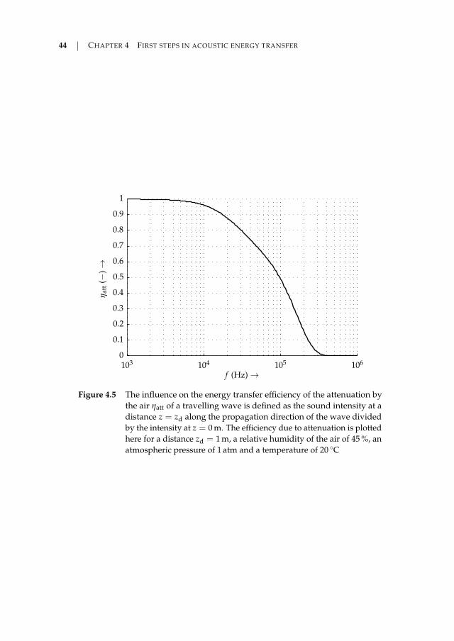
44 CHAPTER 4 FIRST STEPS IN ACOUSTIC ENERGY TRANSFER
ηatt
(−)→
f (Hz) →103 104 105 1060
0.1
0.2
0.3
0.4
0.5
0.6
0.7
0.8
0.9
1
Figure 4.5 The influence on the energy transfer efficiency of the attenuation bythe air ηatt of a travelling wave is defined as the sound intensity at adistance z = zd along the propagation direction of the wave dividedby the intensity at z = 0 m. The efficiency due to attenuation is plottedhere for a distance zd = 1 m, a relative humidity of the air of 45 %, anatmospheric pressure of 1 atm and a temperature of 20 C
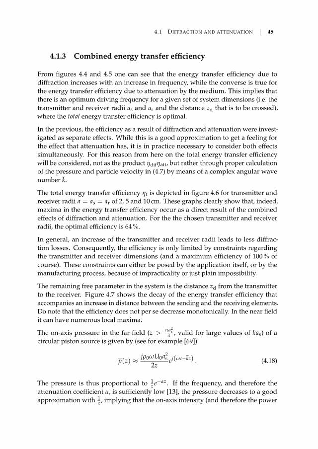
4.1 DIFFRACTION AND ATTENUATION 45
4.1.3 Combined energy transfer efficiency
From figures 4.4 and 4.5 one can see that the energy transfer efficiency due todiffraction increases with an increase in frequency, while the converse is true forthe energy transfer efficiency due to attenuation by the medium. This implies thatthere is an optimum driving frequency for a given set of system dimensions (i.e. thetransmitter and receiver radii as and ar and the distance zd that is to be crossed),where the total energy transfer efficiency is optimal.
In the previous, the efficiency as a result of diffraction and attenuation were invest-igated as separate effects. While this is a good approximation to get a feeling forthe effect that attenuation has, it is in practice necessary to consider both effectssimultaneously. For this reason from here on the total energy transfer efficiencywill be considered, not as the product ηdifηatt, but rather through proper calculationof the pressure and particle velocity in (4.7) by means of a complex angular wavenumber k.
The total energy transfer efficiency ηt is depicted in figure 4.6 for transmitter andreceiver radii a = as = ar of 2, 5 and 10 cm. These graphs clearly show that, indeed,maxima in the energy transfer efficiency occur as a direct result of the combinedeffects of diffraction and attenuation. For the the chosen transmitter and receiverradii, the optimal efficiency is 64 %.
In general, an increase of the transmitter and receiver radii leads to less diffrac-tion losses. Consequently, the efficiency is only limited by constraints regardingthe transmitter and receiver dimensions (and a maximum efficiency of 100 % ofcourse). These constraints can either be posed by the application itself, or by themanufacturing process, because of impracticality or just plain impossibility.
The remaining free parameter in the system is the distance zd from the transmitterto the receiver. Figure 4.7 shows the decay of the energy transfer efficiency thataccompanies an increase in distance between the sending and the receiving elements.Do note that the efficiency does not per se decrease monotonically. In the near fieldit can have numerous local maxima.
The on-axis pressure in the far field (z > πa2s
λ , valid for large values of kas) of acircular piston source is given by (see for example [69])
p(z) ≈ jρ0ωU0a2s
2zej(ωt−kz) . (4.18)
The pressure is thus proportional to 1z e−αz. If the frequency, and therefore the
attenuation coefficient α, is sufficiently low [13], the pressure decreases to a goodapproximation with 1
z , implying that the on-axis intensity (and therefore the power
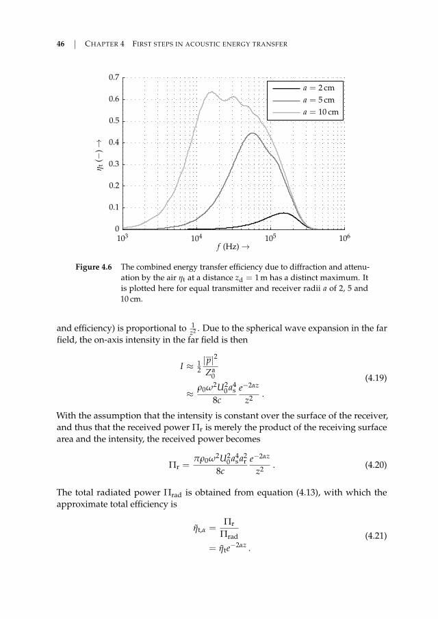
46 CHAPTER 4 FIRST STEPS IN ACOUSTIC ENERGY TRANSFER
a = 10 cm
a = 5 cm
a = 2 cm
ηt
(−)→
f (Hz) →103 104 105 1060
0.1
0.2
0.3
0.4
0.5
0.6
0.7
Figure 4.6 The combined energy transfer efficiency due to diffraction and attenu-ation by the air ηt at a distance zd = 1 m has a distinct maximum. Itis plotted here for equal transmitter and receiver radii a of 2, 5 and10 cm.
and efficiency) is proportional to 1z2 . Due to the spherical wave expansion in the far
field, the on-axis intensity in the far field is then
I ≈ 12|p|2
Za0
≈ρ0ω2U2
0 a4s
8ce−2αz
z2 .
(4.19)
With the assumption that the intensity is constant over the surface of the receiver,and thus that the received power Πr is merely the product of the receiving surfacearea and the intensity, the received power becomes
Πr =πρ0ω2U2
0 a4s a2
r8c
e−2αz
z2 . (4.20)
The total radiated power Πrad is obtained from equation (4.13), with which theapproximate total efficiency is
ηt,α =Πr
Πrad
= ηte−2αz .(4.21)
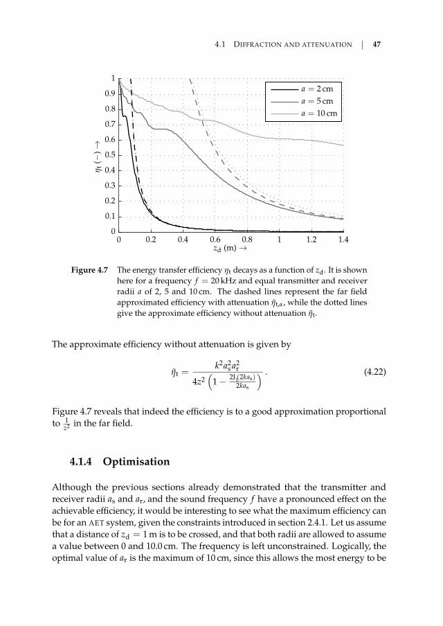
4.1 DIFFRACTION AND ATTENUATION 47
a = 10 cm
a = 5 cm
a = 2 cmη
t(−
)→
zd (m) →0 0.2 0.4 0.6 0.8 1 1.2 1.4
0
0.1
0.2
0.3
0.4
0.5
0.6
0.7
0.8
0.9
1
Figure 4.7 The energy transfer efficiency ηt decays as a function of zd. It is shownhere for a frequency f = 20 kHz and equal transmitter and receiverradii a of 2, 5 and 10 cm. The dashed lines represent the far fieldapproximated efficiency with attenuation ηt,α, while the dotted linesgive the approximate efficiency without attenuation ηt.
The approximate efficiency without attenuation is given by
ηt =k2a2
s a2r
4z2(
1− 2J1(2kas)2kas
) . (4.22)
Figure 4.7 reveals that indeed the efficiency is to a good approximation proportionalto 1
z2 in the far field.
4.1.4 Optimisation
Although the previous sections already demonstrated that the transmitter andreceiver radii as and ar, and the sound frequency f have a pronounced effect on theachievable efficiency, it would be interesting to see what the maximum efficiency canbe for an AET system, given the constraints introduced in section 2.4.1. Let us assumethat a distance of zd = 1 m is to be crossed, and that both radii are allowed to assumea value between 0 and 10.0 cm. The frequency is left unconstrained. Logically, theoptimal value of ar is the maximum of 10 cm, since this allows the most energy to be

48 CHAPTER 4 FIRST STEPS IN ACOUSTIC ENERGY TRANSFER
captured, and hence the diffraction losses to be lowest, assuming, of course, that anincrease in receiver size does not contribute to an increase in its losses.
The optimal values of the remaining two parameters can be found by minimisingthe power loss ratio:
arg minas∈U , f∈R+
(1− ηt) , U := (0; 10] cm . (4.23)
Doing so for a distance zd = 1 m, for example by means of the MATLAB fminsearchoptimisation routine, yields the values as = 7.83 cm and f = 20.53 kHz. Thecorresponding maximum efficiency at 1 m distance is 65.0 %. Recollecting the 64 %that the model predicts in the case of as = ar = 10 cm, the gain in efficiency throughoptimisation is only marginal.
Construction of solid piezo transducers with these desired radii of 7.83 cm and10 cm is quite impractical. It is difficult to design transducers of these sizes thatare sufficiently rigid at the desired frequency of 20 kHz or higher. One possiblesolution is the construction of a transducer array, in which a large number of smalltransducers approximate the desired active surface. The advantage of using atransducer array over a single element is that it can be used for beam steering.This principle is commonly used in medical ultrasonography (it is also used inphased array radar applications). Beam steering can be used in AET applications toovercome low output power due to misalignment of the transmitter and receiver.This is necessary when the location of the transmitter and the receiver is not fixed,or otherwise a priori unknown.
4.2 Transducer efficiency
The last important loss component in an AET system is that which occurs in thetransmitter and the receiver. These transducers can be quite efficient. According toe.g. [66], no more than 10 % losses should be expected when using bending modepiezoelectric transducers that are mounted on the first nodal circle. This constructionhas the advantage of having a high mechanical quality factor of the mounting. Still,often a considerable part of the energy that is lost in AET is due to the losses in thetransmitting and receiving transducers. A good model of the transducer is thereforeof the essence to be able to estimate the total losses in an AET system.
Equivalent electrical networks, such as introduced in section 3.6, are a convenientmethod of describing the behaviour of a transducer (see [17, 65, 75, 87, 101, 117,123, 124]) and can therefore be used to assess the losses that occur in the energy
4.2 TRANSDUCER EFFICIENCY 49
conversion process between the electrical and mechanical domains. Althoughthe circuit can only describe a one-dimensional model, as was explained earlier,equivalent circuits can still be of value for determining the losses in actuators. Theywill allow us to express the efficiency of a transducer in terms of its quality factorsand resonance frequency.
Piezoelectric transducers
Piezoelectric crystals exhibit a net polarisation, which is caused by an atomic latticethat does not have a centre of symmetry [49, 103]. Such atomic lattices can befound for example in naturally occurring crystals such as quartz and tourmaline.The polarisation of the material means that it can be deformed by application ofan electric field, or inversely, that an electric field is created by deforming thecrystal. The result is a linear interaction between its electrical and mechanicalparameters [49, 57, 103].
A piezoelectric actuator generally vibrates in multiple directions. These vibrationsrequire a six-dimensional description; its strain has three normal components (Sxx,Syy and Szz) and three shear components (Sxy, Sxz and Syz). Likewise the stress ina piezoelectric material has the components Txx, Tyy, Tzz, Txy, Txz and Tyz [49, 63].Piezoelectric crystals are usually analysed in terms of tensors, which allow for thedescription of behaviour with multiple degrees of freedom that is required.
The dynamical behaviour of a piezoelectric transducer can be captured in a limitedfrequency range in an electrical equivalent network as depicted in figure 4.8. Itmodels the air load on the diaphragm by a dissipative component Ra and a reactivecomponent Xa. The mechanical part of the transducer is modelled by a resistive, amass, and a compliance component (Rm, Lm and Cm respectively). The mechanicaldomain is coupled to an electrical section through a transformer. The electrical do-main contains a capacitor Ce to account for the capacitive behaviour of a piezoelectricelement, and a resistance Re that models the ceramic’s dielectric losses.
Contrarily to the tensor description, we have only a one-dimensional model in thiscase, as it describes the transducer’s velocity as a scalar quantity u. Although thematerial of the transducer typically vibrates in all six directions, the vibration in onesingle direction is often dominant, which justifies the description of the transducer’sbehaviour by means of a one-dimensional model.
The transformer with transfer ratio ϕ in figure 4.8 originates from the behaviour ofa piezoelectric crystal. The change in electric displacement field due to a strain Sis DS = eS, and the developed stress due to an electric field E is TE = eE [49, 57].The parameter e is the piezoelectric stress constant. Inclusion of the dielectric prop-erties of the material and the compliance of the material results in the constitutive

50 CHAPTER 4 FIRST STEPS IN ACOUSTIC ENERGY TRANSFER
LmCmi uRm
Ra
jXa
1 : ϕ
v
+
−
Fm
+
−
F
+
−
Re Ce
Figure 4.8 The behaviour of a piezoelectric transducer around its resonance fre-quency can be captured in an equivalent electrical circuit.
piezoelectric relations
D = eS + εSE (4.24a)
T = cES− eE . (4.24b)
Here εS is the material’s permittivity for constant strain, and cE is the elastic constantfor constant electric field. Considering a section of the material of length l and areaA, the current due to a strain S is given by iS = A dDS
dt = eAl u, and the force due to
an applied electric field is FE = TE A = eAl v. Hence the relationship between the
mechanical and electrical domain is described by a transformer with a transfer ratioϕ = eA
l for a simple 33-mode actuator in which the strain is uniform throughout thematerial. The coupling between both domains can even by described by means ofa transformer in cases where this last requirement does not hold, as explained ine.g. [65, 94].
Lorentz force transducers
The most common loudspeakers that are in use today for sound reproduction are ofthe voice coil type. These are in fact Lorentz force actuators. Ribbon loudspeakersfall into this category as well, as their principle of operation is exactly the same; theyconsist of a conductive material that is suspended in a magnetic field. The materialexperiences a force when a current is passed through it. In the case of a voicecoil loudspeaker the conductive material is a copper coil, which is mechanicallyconnected to a cone, while the material in a ribbon speaker is a thin foil that servesdirectly as the radiating surface. For more information, see [15, 20, 87, 101] forexample.
Just as is the case for piezoelectric transducers, the behaviour of a Lorentz forceactuator is easily captured in an equivalent circuit diagram, which is shown in figure4.9. Not very surprisingly, its circuit diagram is remarkably similar to figure 4.8.
Let us assume that we have a voice coil actuator with a coil conductor length lsuspended in a homogeneous magnetic field of flux density B, moving at a velocity
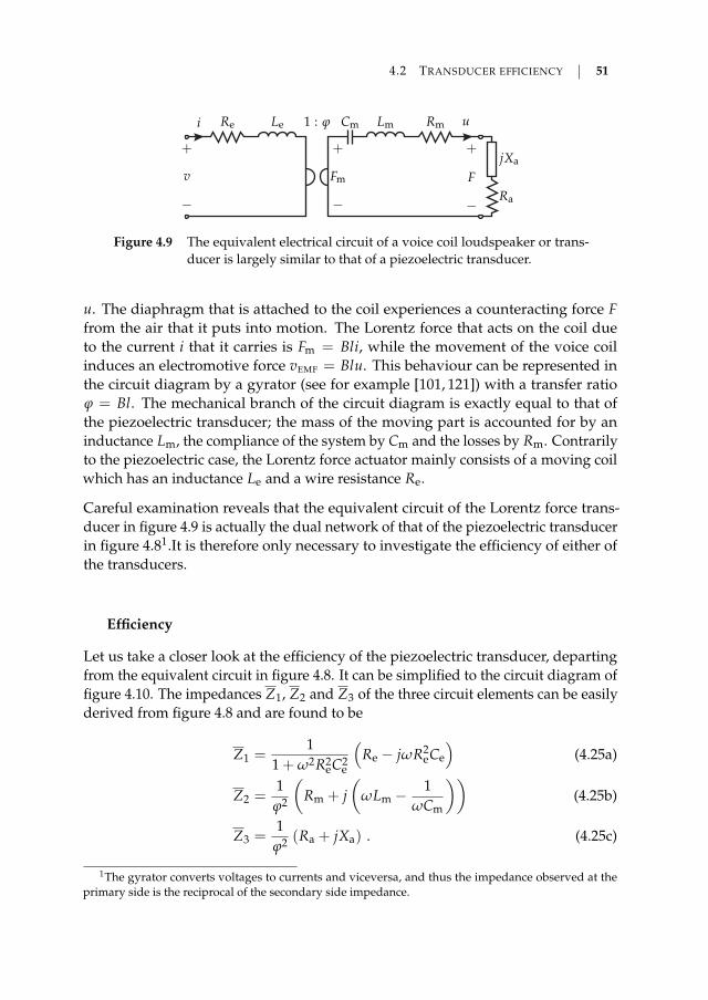
4.2 TRANSDUCER EFFICIENCY 51
LmCmi uRm
Ra
jXa
1 : ϕ
v
+
−
Fm
+
−
F
+
−
Re Le
Figure 4.9 The equivalent electrical circuit of a voice coil loudspeaker or trans-ducer is largely similar to that of a piezoelectric transducer.
u. The diaphragm that is attached to the coil experiences a counteracting force Ffrom the air that it puts into motion. The Lorentz force that acts on the coil dueto the current i that it carries is Fm = Bli, while the movement of the voice coilinduces an electromotive force vEMF = Blu. This behaviour can be represented inthe circuit diagram by a gyrator (see for example [101, 121]) with a transfer ratioϕ = Bl. The mechanical branch of the circuit diagram is exactly equal to that ofthe piezoelectric transducer; the mass of the moving part is accounted for by aninductance Lm, the compliance of the system by Cm and the losses by Rm. Contrarilyto the piezoelectric case, the Lorentz force actuator mainly consists of a moving coilwhich has an inductance Le and a wire resistance Re.
Careful examination reveals that the equivalent circuit of the Lorentz force trans-ducer in figure 4.9 is actually the dual network of that of the piezoelectric transducerin figure 4.81.It is therefore only necessary to investigate the efficiency of either ofthe transducers.
Efficiency
Let us take a closer look at the efficiency of the piezoelectric transducer, departingfrom the equivalent circuit in figure 4.8. It can be simplified to the circuit diagram offigure 4.10. The impedances Z1, Z2 and Z3 of the three circuit elements can be easilyderived from figure 4.8 and are found to be
Z1 =1
1 + ω2R2eC2
e
(Re − jωR2
eCe
)(4.25a)
Z2 =1ϕ2
(Rm + j
(ωLm −
1ωCm
))(4.25b)
Z3 =1ϕ2 (Ra + jXa) . (4.25c)
1The gyrator converts voltages to currents and viceversa, and thus the impedance observed at theprimary side is the reciprocal of the secondary side impedance.

52 CHAPTER 4 FIRST STEPS IN ACOUSTIC ENERGY TRANSFER
+
−v Z1
Z2
Z3
i1i2
+
−v3
Figure 4.10 A simplified equivalent electrical circuit of a piezoelectric transducerdriven by a voltage source.
The power dissipated in every impedance is then
Πn = 12 Re(vn ı∗n) , ∀n ∈ 1, 2, 3 , (4.26)
with vn the voltage across impedance Zn and ın the current through it. From thisnetwork we have for the power Π1, Π2 and Π3, and the efficiency ηtr
Π1 =Re(Z1)
2∣∣Z1∣∣2 |v|2 (4.27a)
Π2 =Re(Z2)
2∣∣Z2 + Z3
∣∣2 |v|2 (4.27b)
Π3 =Re(Z3)
2∣∣Z2 + Z3
∣∣2 |v|2 (4.27c)
ηtr = Π3
(3
∑n=1
Πn
)−1
, (4.27d)
which, after some algebraic manipulation, brings us to
ηtr =ϕ2RaRe
(Rm + Ra)2 +
(ωLm − 1
ωCm+ Xa
)2+ ϕ2Re (Rm + Ra)
. (4.28)
The equivalent circuit diagram of the Lorentz force actuator is, as mentioned earlier,the dual circuit of that of the piezoelectric actuator. It is therefore not very astonishingthat the expression for the efficiency in [87] is very similar to that derived above.In fact, upon closer examination it is exactly equivalent when accounting for thesubstitution of impedances by admittances through the use of the dual circuit.
If we now assume that the reactive part of the air loading on the transducer isdominantly mass-like, i.e. Xa = ωLa, the total impedance of the mechanical branchbecomes
Zm = Rt + j(
ωLt −1
ωCm
). (4.29)
4.2 TRANSDUCER EFFICIENCY 53
in which the equivalent total mechanical resistance is given by Rt = Rm + Ra andthe equivalent total mass is Lt = Lm + La.
The output of the piezoelectric transducer will be highest at the mechanical reson-ance frequency ω0, which follows from the condition d
dω |Zm| = 0 and gives
ω20 =
1LtCm
. (4.30)
The expression for the efficiency in (4.28) is quite obscure, and it does not serve muchpurpose in gaining insight into the behaviour of a transducer. This can be somewhatimproved by rewriting it in terms of the resonance frequency, given above, and itsquality factors. Let us introduce firstly a mechanical quality factor Qm, which relatesthe mechanically dissipated energy to the stored mechanical energy. The latter isstored in the resonant circuit formed by Lt and Cm;
Estored,m(t) = 12 Ltu2(t) + 1
2 CmF2C(t) . (4.31)
The force FC is the ‘voltage’ across the capacitance Cm, or, equivalently, the netforce acting on the lumped element compliance of the transducer. At the resonancefrequency the stored energy is constant and equal to
Estored,m = 12 LtU2 , (4.32)
with U the amplitude of the transducer’s velocity. The power that is dissipated inthe mechanical resistance Rt is given by Pdiss,m = 1
2 RtU2, and thus the energy thatis dissipated in a single cycle is
Ediss,m =2π
ωPdiss,m . (4.33)
This yields a mechanical quality factor
Qm = 2πEstored,m
Ediss,m=
1Rt
√Lt
Cm. (4.34)
The mechanical losses in the resistances Rm and Ra are not the only losses in thetransducer. The losses in the electrical resistance Re should be considered as well.Doing so leads to the definition of an electrical quality factor Qe, in analogous fashionto [117]. The power dissipated in the resistance is equal to Pdiss,e = 1
2 R2t /ϕ2ReU2,
which renders the electrical quality factor
Qe = 2πEstored,m
Ediss,e=
ϕ2Re
R2t
√Lt
Cm. (4.35)

54 CHAPTER 4 FIRST STEPS IN ACOUSTIC ENERGY TRANSFER
These definitions allow the efficiency of the piezoelectric transducer in equation(4.28) to be written in a somewhat simpler form as
ηtr =
QeQm
1 + QeQm
+(
ωω0− ω0
ω
)2Q2
m
Ra
Ra + Rm(4.36)
This equation is, after minor rearrangement of terms, equal to that of a voice coilloudspeaker [2], which is expected, given the duality of the equivalent circuitsof both transducer types. Note that all parameters in (4.36) can be derived fromthe electrical impedance seen at the electrical port of the transducer. From elec-trical impedance measurements one cannot separate Ra from Rm and Xa from(ωLm − 1/ωCm). However, it is possible to measure these components indirectly, bymeasuring the impedance under two loading conditions; operating in air, and invacuum (which effectively shorts the air load Ra + jXa), or using another a prioriknow acoustic load.
Unlike traditional loudspeakers, the electrical losses can often be neglected in piezo-electric transducers. A traditional voicecoil loudspeaker suffers from the resistiveloss in its copper coil. This coil is traditionally designed to be extremely lightweightsince it should not add significant mass to that of the cone and the air it displaces [20].The resulting voice coil design is therefore a tradeoff between losses and addedmass. This is not to say that Lorentz force actuators with low electrical losses cannotbe constructed. The electrical losses in a piezoelectric transducer, on the other hand,are mostly of dielectric nature. These are normally insignificant for piezoelectricmaterials. Discarding the electrical losses changes the expression for the efficiencyof the transducer (4.36) to the somewhat unsurprising result
limQe→∞
ηtr =Ra
Ra + Rm, (4.37)
which is again equivalent to the approximation in [2] for a large value of Bl.
Operation as a receiver
The equivalent circuits of the piezoelectric and Lorentz force actuator are in principlereversible; decoupling the air load Ra and Xa and applying a force or velocity willproduce a corresponding voltage v at the electrical port. Connection of an electricalload between the terminals will then also allow a current i to flow.
The efficiency of a receiver is easily calculated in much the same manner as itwas derived for the transmitter. Its equivalent circuit diagram can be simplifiedto that depicted in figure 4.11, where the impedance of the mechanical branch is

4.2 TRANSDUCER EFFICIENCY 55
+
−v jX2 R2
i2
Z1 i1
Figure 4.11 A simplified equivalent electrical circuit of a piezoelectric transduceroperating as a receiving element.
Z1 = Rm + j (ωLm − 1/ωCm), the electrical reactance is X2 = 1/ωCe and the electricalresistance is 1/(ϕ2R2
)= 1/Re + 1/RL. The resistance RL is the load resistance that is
connected to the electrical terminals. It is easy enough to show that the efficiency ofthe transducer in this case is
ηtr =R2
Rm + R2 +RmR2
2X2
2
. (4.38)
Interestingly enough, the efficiency of the receiving transducer does not depend onthe mass nor on the compliance of the transducer. Please note that they do influencethe output power, since the current i1 depends on the total value of Z1 + (R2 ‖ jX2),which is at a maximum at the resonance frequency ω0 = 1√
LmCm. This resonance
frequency can be different from that of the transmitting transducer, where theradiation reactance Xa also plays a role in the resonance frequency (cf. equation(4.30)). A different resonance frequency can be problematic if both transducers havea very high quality factor, which would lead to a low energy transfer in the caseof a frequency mismatch. This tends to be less of a problem for larger transducers,as can be gathered from figure 4.3, since Xa approaches 0 for large values of kas,which is ratio of the transducer circumference to the wavelength. In other situationsone should take care through proper design of the transducers that the resonancefrequency of the transmitter and the receiver match.
The only frequency dependent component in (4.38) is introduced by the electricalreactance X2, and thus the electrical capacitance Ce of the piezo element. Theefficiency of the receiver will be optimal if we can make X2 approach an infinitevalue. In that case the efficiency of the transducer becomes
limX2→∞
ηtr =R2
Rm + R2. (4.39)
Or, when neglecting the dielectric losses, the expression reduces even further to
limX2→∞Re→∞
ηtr =ϕ2RL
Rm + ϕ2RL. (4.40)
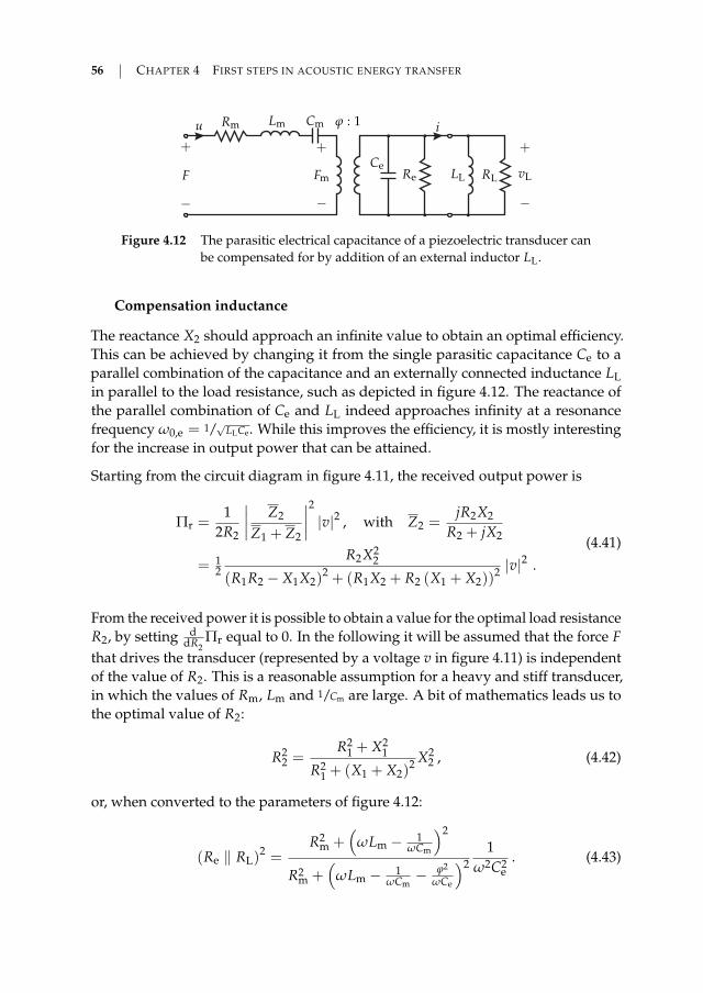
56 CHAPTER 4 FIRST STEPS IN ACOUSTIC ENERGY TRANSFER
ReCe
Lm Cm iu Rm
RLLL
ϕ : 1
vL
+
−
Fm
+
−
F
+
−
Figure 4.12 The parasitic electrical capacitance of a piezoelectric transducer canbe compensated for by addition of an external inductor LL.
Compensation inductance
The reactance X2 should approach an infinite value to obtain an optimal efficiency.This can be achieved by changing it from the single parasitic capacitance Ce to aparallel combination of the capacitance and an externally connected inductance LLin parallel to the load resistance, such as depicted in figure 4.12. The reactance ofthe parallel combination of Ce and LL indeed approaches infinity at a resonancefrequency ω0,e = 1/√LLCe. While this improves the efficiency, it is mostly interestingfor the increase in output power that can be attained.
Starting from the circuit diagram in figure 4.11, the received output power is
Πr =1
2R2
∣∣∣∣ Z2
Z1 + Z2
∣∣∣∣2 |v|2 , with Z2 =jR2X2
R2 + jX2
= 12
R2X22
(R1R2 − X1X2)2 + (R1X2 + R2 (X1 + X2))
2 |v|2 .
(4.41)
From the received power it is possible to obtain a value for the optimal load resistanceR2, by setting d
dR2Πr equal to 0. In the following it will be assumed that the force F
that drives the transducer (represented by a voltage v in figure 4.11) is independentof the value of R2. This is a reasonable assumption for a heavy and stiff transducer,in which the values of Rm, Lm and 1/Cm are large. A bit of mathematics leads us tothe optimal value of R2:
R22 =
R21 + X2
1
R21 + (X1 + X2)
2 X22 , (4.42)
or, when converted to the parameters of figure 4.12:
(Re ‖ RL)2 =
R2m +
(ωLm − 1
ωCm
)2
R2m +
(ωLm − 1
ωCm− ϕ2
ωCe
)21
ω2C2e
. (4.43)
4.2 TRANSDUCER EFFICIENCY 57
In practice one will want to work at the resonance frequency of the system, reducingthe influence of the reactive system components and maximising the excursion ofthe transducers. Following this assumptions allows for the mechanical reactance X1to be set to 0. Therefore, the optimal value of R2 becomes
R22 =
R21X2
2R2
1 + X22
. (4.44)
This renders the output power equal to
Πr =1
4R1
11 +
√1 + R2
1/X22
|v|2 , (4.45)
which, in terms of the parameters of the equivalent circuit diagram in figure 4.12 is
Πr =1
4Rm
1
1 +√
1 + R2mC2
eϕ2LmCm
|F|2 , (4.46)
If the resistance R1 is large in comparison to X2, or R1/X2 1, the output powerapproaches
Πr ≈1
4R1
X2
R1|v|2 ≈ 0 W . (4.47)
On the other hand, compensating the electrical capacitance Ce by means of aninductance (X2 → ∞), the output power (4.45) logically is
limX2→∞
Πr =1
8R1|v|2 =
18Rm
|F|2 . (4.48)
This shows that proper compensation of the electrical capacitance of a piezoelectrictransducer acting as a receiver in an AET system can result in much higher outputpower. However, it also shows that compensation will not improve the performancein systems where the mechanical damping in the transducer is low in comparison tothe reactance presented by the parasitic capacitance:
R1
X2 1 . (4.49)
The load resistance was chosen in this section such that the maximum output poweris obtained. This is not always the best choice, since it inevitably means that 50 %of the received power is lost in the damping of the transducer. If the losses aresufficiently low, or the available power is greater, one could opt to choose a higherload resistance, such that the efficiency is higher, but at the cost of a reduced receivedoutput power.
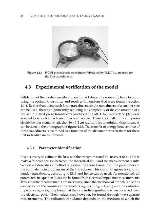
58 CHAPTER 4 FIRST STEPS IN ACOUSTIC ENERGY TRANSFER
Figure 4.13 PX051 piezoelectric transducers fabricated by EMCT SA are used forthe first experiments.
4.3 Experimental verification of the model
Validation of the model described in section 4.1 does not necessarily have to occurusing the optimal transmitter and receiver dimensions that were found in section4.1.4. Rather than using such large transducers, single transducers of a smaller sizecan be used, thereby significantly reducing the complexity of the construction of atest setup. PX051 piezo transducers produced by EMCT SA, Switzerland [32] wereselected to serve both as transmitter and receiver. These are small unimorph piezo-electric bender elements, attached to a 1.2 cm radius, thin, aluminium diaphragm, ascan be seen in the photograph of figure 4.13. The transfer of energy between two ofthese transducers is examined as a function of the distance between them for thesefirst indicative measurements.
4.3.1 Parameter identification
It is necessary to estimate the losses of the transmitter and the receiver to be able tomake a fair comparison between the theoretical limit and the measurement results.Section 4.2 describes a method of estimating these losses from the parameters ofthe equivalent circuit diagram of the transducer. This circuit diagram is valid forbender transducers, according to [24], and hence can be used. As mentioned, allparameters in equation (4.36) can be found from electrical impedance measurements.Two separate measurements are necessary, since the mechanical branch is a seriesconnection of the transducer parameters Rm + j (ωLm − 1/ωCm) and the radiationimpedance Ra + jXa, implying that they are indistinguishable when observed fromthe electrical port. Their values can, however, be found through two separatemeasurements. The radiation impedance depends on the medium in which the
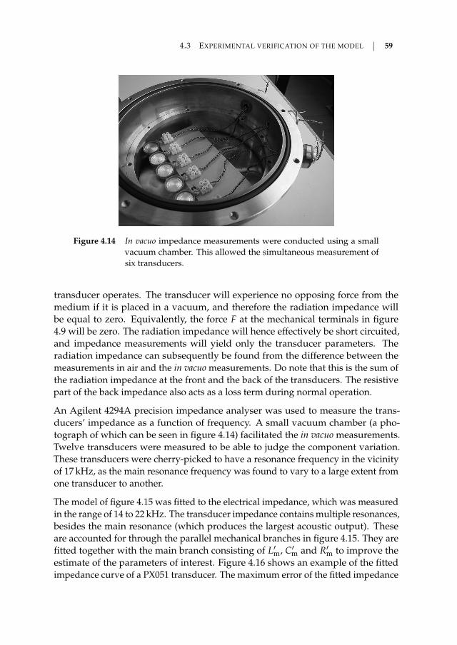
4.3 EXPERIMENTAL VERIFICATION OF THE MODEL 59
Figure 4.14 In vacuo impedance measurements were conducted using a smallvacuum chamber. This allowed the simultaneous measurement ofsix transducers.
transducer operates. The transducer will experience no opposing force from themedium if it is placed in a vacuum, and therefore the radiation impedance willbe equal to zero. Equivalently, the force F at the mechanical terminals in figure4.9 will be zero. The radiation impedance will hence effectively be short circuited,and impedance measurements will yield only the transducer parameters. Theradiation impedance can subsequently be found from the difference between themeasurements in air and the in vacuo measurements. Do note that this is the sum ofthe radiation impedance at the front and the back of the transducers. The resistivepart of the back impedance also acts as a loss term during normal operation.
An Agilent 4294A precision impedance analyser was used to measure the trans-ducers’ impedance as a function of frequency. A small vacuum chamber (a pho-tograph of which can be seen in figure 4.14) facilitated the in vacuo measurements.Twelve transducers were measured to be able to judge the component variation.These transducers were cherry-picked to have a resonance frequency in the vicinityof 17 kHz, as the main resonance frequency was found to vary to a large extent fromone transducer to another.
The model of figure 4.15 was fitted to the electrical impedance, which was measuredin the range of 14 to 22 kHz. The transducer impedance contains multiple resonances,besides the main resonance (which produces the largest acoustic output). Theseare accounted for through the parallel mechanical branches in figure 4.15. They arefitted together with the main branch consisting of L′m, C′m and R′m to improve theestimate of the parameters of interest. Figure 4.16 shows an example of the fittedimpedance curve of a PX051 transducer. The maximum error of the fitted impedance
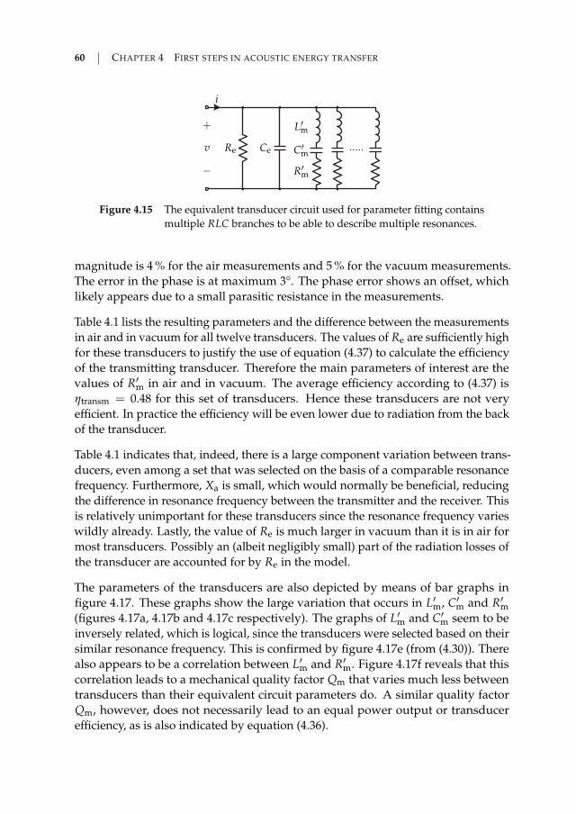
60 CHAPTER 4 FIRST STEPS IN ACOUSTIC ENERGY TRANSFER
L′m
C′m
i
R′m
v
+
−
Re Ce
Figure 4.15 The equivalent transducer circuit used for parameter fitting containsmultiple RLC branches to be able to describe multiple resonances.
magnitude is 4 % for the air measurements and 5 % for the vacuum measurements.The error in the phase is at maximum 3°. The phase error shows an offset, whichlikely appears due to a small parasitic resistance in the measurements.
Table 4.1 lists the resulting parameters and the difference between the measurementsin air and in vacuum for all twelve transducers. The values of Re are sufficiently highfor these transducers to justify the use of equation (4.37) to calculate the efficiencyof the transmitting transducer. Therefore the main parameters of interest are thevalues of R′m in air and in vacuum. The average efficiency according to (4.37) isηtransm = 0.48 for this set of transducers. Hence these transducers are not veryefficient. In practice the efficiency will be even lower due to radiation from the backof the transducer.
Table 4.1 indicates that, indeed, there is a large component variation between trans-ducers, even among a set that was selected on the basis of a comparable resonancefrequency. Furthermore, Xa is small, which would normally be beneficial, reducingthe difference in resonance frequency between the transmitter and the receiver. Thisis relatively unimportant for these transducers since the resonance frequency varieswildly already. Lastly, the value of Re is much larger in vacuum than it is in air formost transducers. Possibly an (albeit negligibly small) part of the radiation losses ofthe transducer are accounted for by Re in the model.
The parameters of the transducers are also depicted by means of bar graphs infigure 4.17. These graphs show the large variation that occurs in L′m, C′m and R′m(figures 4.17a, 4.17b and 4.17c respectively). The graphs of L′m and C′m seem to beinversely related, which is logical, since the transducers were selected based on theirsimilar resonance frequency. This is confirmed by figure 4.17e (from (4.30)). Therealso appears to be a correlation between L′m and R′m. Figure 4.17f reveals that thiscorrelation leads to a mechanical quality factor Qm that varies much less betweentransducers than their equivalent circuit parameters do. A similar quality factorQm, however, does not necessarily lead to an equal power output or transducerefficiency, as is also indicated by equation (4.36).
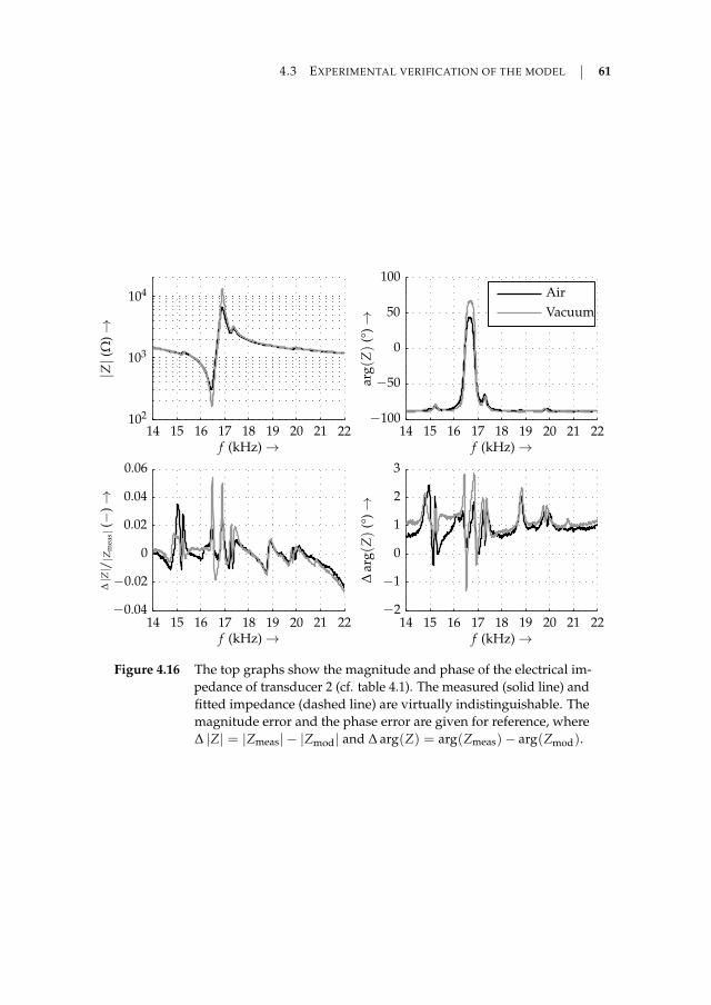
4.3 EXPERIMENTAL VERIFICATION OF THE MODEL 61
∆ar
g(Z
)(°
)→
f (kHz) →
∆|Z| /
|Zm
eas|(−
)→
f (kHz) →
Vacuum
Air
arg(Z
)(°
)→
f (kHz) →
|Z|
(Ω)→
f (kHz) →
14 15 16 17 18 19 20 21 2214 15 16 17 18 19 20 21 22
14 15 16 17 18 19 20 21 2214 15 16 17 18 19 20 21 22
−2
−1
0
1
2
3
−0.04
−0.02
0
0.02
0.04
0.06
−100
−50
0
50
100
102
103
104
Figure 4.16 The top graphs show the magnitude and phase of the electrical im-pedance of transducer 2 (cf. table 4.1). The measured (solid line) andfitted impedance (dashed line) are virtually indistinguishable. Themagnitude error and the phase error are given for reference, where∆ |Z| = |Zmeas| − |Zmod| and ∆ arg(Z) = arg(Zmeas)− arg(Zmod).
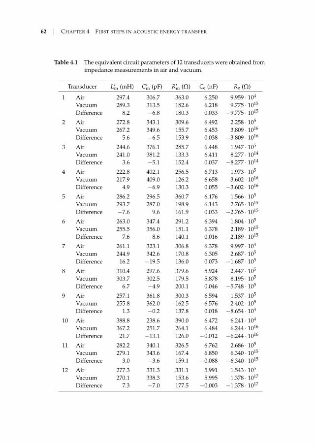
62 CHAPTER 4 FIRST STEPS IN ACOUSTIC ENERGY TRANSFER
Table 4.1 The equivalent circuit parameters of 12 transducers were obtained fromimpedance measurements in air and vacuum.
Transducer L′m (mH) C′m (pF) R′m (Ω) Ce (nF) Re (Ω)
1 Air 297.4 306.7 363.0 6.250 9.959 · 104
Vacuum 289.3 313.5 182.6 6.218 9.775 · 1015
Difference 8.2 −6.8 180.3 0.033 −9.775 · 1015
2 Air 272.8 343.1 309.6 6.492 2.258 · 105
Vacuum 267.2 349.6 155.7 6.453 3.809 · 1016
Difference 5.6 −6.5 153.9 0.038 −3.809 · 1016
3 Air 244.6 376.1 285.7 6.448 1.947 · 105
Vacuum 241.0 381.2 133.3 6.411 8.277 · 1014
Difference 3.6 −5.1 152.4 0.037 −8.277 · 1014
4 Air 222.8 402.1 256.5 6.713 1.973 · 105
Vacuum 217.9 409.0 126.2 6.658 3.602 · 1016
Difference 4.9 −6.9 130.3 0.055 −3.602 · 1016
5 Air 286.2 296.5 360.7 6.176 1.566 · 105
Vacuum 293.7 287.0 198.9 6.143 2.765 · 1015
Difference −7.6 9.6 161.9 0.033 −2.765 · 1015
6 Air 263.0 347.4 291.2 6.394 1.804 · 105
Vacuum 255.5 356.0 151.1 6.378 2.189 · 1015
Difference 7.6 −8.6 140.1 0.016 −2.189 · 1015
7 Air 261.1 323.1 306.8 6.378 9.997 · 104
Vacuum 244.9 342.6 170.8 6.305 2.687 · 105
Difference 16.2 −19.5 136.0 0.073 −1.687 · 105
8 Air 310.4 297.6 379.6 5.924 2.447 · 105
Vacuum 303.7 302.5 179.5 5.878 8.195 · 105
Difference 6.7 −4.9 200.1 0.046 −5.748 · 105
9 Air 257.1 361.8 300.3 6.594 1.537 · 105
Vacuum 255.8 362.0 162.5 6.576 2.402 · 105
Difference 1.3 −0.2 137.8 0.018 −8.654 · 104
10 Air 388.8 238.6 390.0 6.472 6.241 · 104
Vacuum 367.2 251.7 264.1 6.484 6.244 · 1016
Difference 21.7 −13.1 126.0 −0.012 −6.244 · 1016
11 Air 282.2 340.1 326.5 6.762 2.686 · 105
Vacuum 279.1 343.6 167.4 6.850 6.340 · 1015
Difference 3.0 −3.6 159.1 −0.088 −6.340 · 1015
12 Air 277.3 331.3 331.1 5.991 1.543 · 105
Vacuum 270.1 338.3 153.6 5.995 1.378 · 1017
Difference 7.3 −7.0 177.5 −0.003 −1.378 · 1017

4.3 EXPERIMENTAL VERIFICATION OF THE MODEL 63
L′ m
(mH
)→
Transducer →
1 2 3 4 5 6 7 8 9 10 11 120
50
100
150
200
250
300
350
400
(a)
C′ m
(pF
)→
Transducer →1 2 3 4 5 6 7 8 9 10 11 12
0
50
100
150
200
250
300
350
400
450
(b)
R′ m
(Ω)→
Transducer →
1 2 3 4 5 6 7 8 9 10 11 120
50
100
150
200
250
300
350
400
(c)
Ce
(nF
)→
Transducer →
1 2 3 4 5 6 7 8 9 10 11 120
1
2
3
4
5
6
7
8
(d)
f 0(k
Hz)→
Transducer →
1 2 3 4 5 6 7 8 9 10 11 120
2
4
6
8
10
12
14
16
18
20
(e)
Qm
(−)→
Transducer →
1 2 3 4 5 6 7 8 9 10 11 120
20
40
60
80
100
120
140
160
180
200
(f)
Figure 4.17 Bar plots of the transducer parameters clearly show the parametervariation, even though the transducers were cherry-picked. Theblack bars represent the impedance measurements in air, and thegrey graphs those in vacuum.
64 CHAPTER 4 FIRST STEPS IN ACOUSTIC ENERGY TRANSFER
4.3.2 Setup
One of the assumptions made during the derivation of the model is the coaxial place-ment of the transducers, just as in the system of figure 4.1. Consequently, an accuratealignment of the transmitting and receiving transducers is required. Furthermore,the distance between the two is to be accurately measured and precisely controlledfor these measurements. This is achieved through the use of a milling machineas a means for distance variation between, and alignment of the transducers. Aphotograph of the setup can be seen in figure 4.18. The machine is fitted with a linearencoder system that has an accuracy of 10 µm, which should be adequate, given thatthe resonance frequency at which the transducers are used is approximately 17 kHz,implying a wavelength λ = 20 mm. The resolution of the positioning system istherefore orders of magnitude smaller than the wavelength.
Care should be taken when doing such measurements that the vibrations of thetransmitter only couple with the receiver via the medium (the air in this case) andnot via the platform on which they are mounted. The coupling via the millingmachine is nil in this case. Therefore all received power can be considered to havebeen transferred through the air.
Due to their physical construction the PX051 transducers are not suited for highpower levels. This shows in low voltages and particularly low current amplitudes(i.e. tenths of milliamperes). Amplification is therefore necessary to properly measurethe currents. Care should be taken that the amplifier does not introduce an error inthe power measurements. An amplifier always inserts a certain phase shift betweenits input and output signal. Since we are concerned with power measurements, thephase relation between the transducer’s voltage and current is of importance andshould be maintained. This is achieved in this setup by using an identical amplifiercircuit for the measurement of the transducers’ voltages and their currents. Theoutput of the amplifiers is measured with a LeCroy WaveRunner 44Xi oscilloscope,which calculates the power as the cyclic average of the product of the voltage andcurrent.
The transducers were used at their mechanical resonance frequency ω0. Since thereactive component Xa of the radiation impedance is negligible, the resonancefrequencies of the transmitter and the receiver are approximately equal.
The load resistance RL was varied to obtain maximum power transfer, which resultedin an optimal value of RL = 1990.3 Ω. A compensation inductance was used, asdescribed in section 4.2 to maximise the power output at the receiving side. Frommeasurements with an Agilent 4294A impedance analyser the resonance frequencyof a freely radiating PX051 transducer is measured to be f0 = ω0
2π = 17.0 kHz. Themeasurements of energy transfer efficiency versus distance were therefore conducted

4.3 EXPERIMENTAL VERIFICATION OF THE MODEL 65
Figure 4.18 Two PX051 transducers are mounted on a milling machine to facilitateaccurate alignment and distance variation.
at this frequency. The electric capacitance of the piezo transducer was measured tobe approximately Ce = 6.0 nF. Therefore an inductor of LL = 15 mH was used tomake the resonance frequency of the LL-Ce combination equal to the mechanicalresonance frequency ω0.
The input power was delivered by an arbitrary waveform generator. No outputrectifier was used at the receiving side for the sake of simplicity, since our interestlies primarily with the energy transfer by means of sound waves and not as muchwith the influence of the electrical circuitry.
4.3.3 Measurement results
Figure 4.19a shows the measured efficiency of the energy transfer between anidentical transmitting and receiving piezo element. The efficiency is measured as theratio of average electrical output power of the receiving transducer to the averageelectrical input power of the transmitting transducer. The graph also includes thetheoretical limit for this setup, which was derived in section 4.1. The theoreticallimit includes a transmitter efficiency ηtransm = 0.48 as determined in section 4.3.1and a receiver efficiency ηrec = 0.50, assuming a perfectly matched load resistance
66 CHAPTER 4 FIRST STEPS IN ACOUSTIC ENERGY TRANSFER
RL. The measured input power Πin and output power Πout are plotted as a functionof the distance zd in figure 4.19b. Separate points are indicated in both graphs wherethe energy transfer was measured at higher power levels. These measurementswere limited by the breakdown voltage of the transmitting piezo element. The inputpower, output power and efficiency that were measured during this maximum-power measurement are
Πin, Max power = 184.9 mW
Πout, Max power = 40.0 mW
η = 21.6 % .
The higher efficiency obtained at maximum power is most likely due to the use of adifferent set of piezo elements with slightly different parameters, as the transducerssuffer heavily from component variation (see also table 4.1). Possibly there was lessdiscrepancy in the resonance frequencies of the transducers for this set, or internallosses were lower for one or both transducer(s).
There are some notable differences between the measured efficiency and the the-oretical limit in figure 4.19a. First and foremost, the efficiency shows a very peakybehaviour, revealing many local maxima and minima as a function of distance.These are a direct result of reflections that occur at the surfaces of both the receivingand the transmitting transducers. A wave that arrives at the face of the transducerbounces into it if the transducer is not moving at the same velocity as the particlesin the wave. This causes the wave to reflect, travelling back to the transmitter, fromwhich it will reflect again, et cetera. This leads to (partial) standing waves, or spatialresonances. Whenever the distance zd is a multiple of the half wavelength 1
2 λ, thetotal phase shift that a sound wave undergoes on a round trip from transmitter toreceiver and back to transmitter is 360 degrees, and thus a resonance occurs. This isthe same effect on the basis of which lasers work, and which occurs in incorrectlyterminated transmission lines. Obviously, reflections are not considered in the modelderived in section 4.1, since the assumption was made that the receiver extracts allthe available energy from the incoming sound wave, prohibiting the existence of areflected wave. Reflections will be discussed in more detail in chapter 5.
Another difference from the theoretical model is found in the level of the measuredefficiency, which decreases decidedly faster than the model predicts. The level ofthe first peak is well approximated by the model, especially for the high powermeasurement (η = 0.2163 from the measurement versus η = 0.2171 predicted by themodel). Consequent peaks are much lower than the modelled efficiency. This canbe attributed to the fact that the pressure and particle velocity change significantlydue to the reflections with respect to that predicted by the simple model describingthe radiation pattern of a circular piston. Moreover, the PX051 transducers have anopen back, as can be seen in figure 4.13), implying that part of the acoustic energy

4.3 EXPERIMENTAL VERIFICATION OF THE MODEL 67
Max power
Measurements
Theoretical limit
η(−
)→
zd (mm) →
0 10 20 30 40 50 60 70 80 90 10010−4
10−3
10−2
10−1
100
(a)
Πout, Max power
Πin, Max power
Πout
Πin
Π(W
)→
zd (mm) →
0 10 20 30 40 50 60 70 80 90 10010−7
10−6
10−5
10−4
10−3
10−2
10−1
100
(b)
Figure 4.19 The source-to-load energy transfer efficiency η of two EMCT PX051piezo transducers was measured as a function of the distance zdbetween them (a). The theoretical limit for this setup is shown forreference. The corresponding measured electrical input and outputpower are shown in (b).The radius of the transducers is 1.2 cm.
68 CHAPTER 4 FIRST STEPS IN ACOUSTIC ENERGY TRANSFER
is radiated from the back of the transmitter and does not contribute to the energytransfer.
Finally, the optimal value of the load resistance RL = 1990.3 Ω was found as theload resistance that yields the highest output power at the first spatial resonancepeak. From (4.44), the assumption that Re is sufficiently high, and a compensatedcapacitance Ce, one expects that RL = Rm/ϕ2 = R′m. Strangely enough, comparisonwith table 4.1 tells us differently. From it one would expect the value of the loadresistance to lie between 125 Ω and 390 Ω 2. The most likely explanation for thisinconsistency would be an inadequate model on the basis of which the optimal loadresistance was derived.
Another possible explanation for the observed difference between the optimal loadresistance and the internal resistance of the transducer is an excessively large valueof R′m, either through component variations or because of a faulty transducer, al-though this seems unlikely judging from the variation encountered in table 4.1. Themaximum value of R′m that was measured was 200.1 Ω.
A last possibility to explain the difference is a measurement error in determiningthe optimal load resistance, which yielded an incorrect value of RL. Since thesemeasurements are quite demanding to perform there is always a possibility thaterrors are made. Some indication in this direction can be found in the results of aseparate set of energy transfer measurements with a different set of transducers,where an optimal load of RL = 420 Ω was found. These measurements wereperformed without compensation inductance. A corresponding value of R′m isfound from (4.44) as
R′m =
√R2
L1−ω2R2
LC2e= 436.1 Ω , (4.50)
with ω = 2π · 17.0 kHz, RL = 420 Ω and Ce = 6.0 nF. Although this value is muchlower than that found in the experiments described above, still it is not low enoughto fall into the range indicated by table 4.1. It is possible that the difference inoptimal load resistance is attributable to the distance between the transmitter andthe receiver at which the maximum output power was sought. The load resistancefor the first set of measurements was determined at the first output power peak,while the second was optimised at zd = 10 cm. Still, the second value is too large tobe able to attribute the high values of RL to a measurement error.
2A transducer loss resistance R′m = 390 Ω implies that all power is radiated from the back of thetransducer, when operating under free radiating conditions, which is certainly not the case. In practice itsvalue will be lower.

4.4 CONCLUSIONS AND DISCUSSION 69
4.4 Conclusions and discussion
The theoretical limit to the energy transfer efficiency of an AET system is derived inthis chapter based on an identification of the losses that occur in such a system. Themodel that it is derived from includes diffraction, attenuation and transducer losses.Optimal electrical loading conditions were derived based on this model.
Acoustic energy transfer achieves a maximum efficiency of 65 % over a distanceof 1 m, when the radii of the transmitter and receiver are restricted to 10 cm. Thistheoretical limit is based on diffraction and attenuation losses only. For the inclusionof transducer losses, one can look at examples of high efficiency transducers suchas found in literature; for example Gallego-Juarez et al. [38], who reported an 82 %efficient high power transducer, or Kritz [66], who published a paper on a 93 %efficient ultrasound transducer. Assuming that the transmitter operates at thelatter efficiency and the receiver is (according to (4.39) and (4.44)) 50 % efficient,the resulting total efficiency limit is 30 %. If the electrical loading of the receivingtransducer is optimised for maximum efficiency, rather than maximum outputpower, even higher efficiencies up to 60 % can be attained.
According to Waffenschmidt & Staring [127], an inductively coupled CET systemwith the same transmitter and receiver dimensions would have an efficiency ofapproximately 2 %, assuming coil quality factors of 1000. Mur-Miranda et al. [84] usea different approach to the maximum energy transfer of an inductive CET systemand arrive at approximately 6 % efficiency for the same dimensions and qualityfactors. Hence AET has the potential to perform at least 5 to 10 times better in termsof efficiency. This advantage of AET over inductive CET grows very rapidly with thedistance that is to be crossed, since the efficiency of AET is approximately inverselyproportional to z 2
d (cf. equation (4.21)), while that of inductive CET is inverselyproportional to z 6
d [84].
The model on which the theoretical limit is based was validated through experimentsin which the energy transfer between two piezoelectric unimorph bender elementswas measured. These first indicative measurements show that energy transfer bymeans of sound waves is feasible. The maximum output power that was reached(40 mW) is a bit too low to be useful for many applications. This can be attributedto the low power handling capabilities of the transducers that were used for theexperiments. There are, however, applications in which power transfer of thisorder of magnitude is quite adequate. Examples that come to mind are poweringremote sensor applications, MEMS (microelectromechanical systems) and chargingbiomedical implants
The measured efficiency and power show a clear influence of reflections of the soundwaves from the faces of the transducers. Both quantities show distinct peaks as a
70 CHAPTER 4 FIRST STEPS IN ACOUSTIC ENERGY TRANSFER
function of the distance between the transmitter and the receiver, correspondingto half-wavelength intervals. These spatial resonances (figure 4.19) can be min-imised by appropriate termination of the acoustic path. Just like a transmissionline, the acoustic impedance of the receiver should be matched to the characteristicimpedance Za
0 of the air. Chapter 5 discusses reflections in more detail. Acousticimpedance transformers, such as diaphragms [15, 20], horns [20, 44, 69, 105, 106, 128],and 1
4 λ-matching layers [17, 41, 64], can be used for this purpose. Diaphragms andhorns are used most widely in combination with air transducers. Both are extens-ively used for audio reproduction among other purposes. Chapters 6 and 7 examinetheir application to acoustic energy transfer.
The measured efficiency corresponds very well to the theoretical limit model at thefirst spatial resonance peak. The decline in efficiency with the distance between bothtransducers proved to be greater in reality than predicted by the model. This is mostlikely due to the pressure and particle velocity distribution being altered drasticallyby the reflections.
Both the calculated efficiency limit and the measured maximum efficiency showgood agreement with those attained by Ozeri et al. [88,90], who reported respectively27 % and 39.1 % over short distances through a very lossy medium. The measuredefficiency, peaking at 21.6 %, is a bit lower. This however, is a quite good result,considering that open back transducers are used and the transducers have not beenoptimised for this purpose
It is clear from the difference between the value of the optimal electric load RLand the value of the mechanical transducer resistance R′m, that the models of thetransducers are not entirely correct. The optimal load resistance was derived underthe assumption that it does not have any influence on the pressure acting on thereceiving transducer. This assumption is in practice not valid. The transducerpresents an equivalent acoustic impedance to the incoming sound wave. Thisimpedance, which depends on the value of the load resistance, determines theoccurrence of reflections and their intensity (see the experimental results in [89]).Therefore it also influences the pressure at the face of the receiver. Hence theassumption that p at the face of the receiver is independent of RL is most likelyinaccurate.
Assuming that the transmitter and the transmission path up to the receiver canbe modelled by a Thévenin equivalent voltage source FTh and series impedanceZa
Th = RTh + jXTh, the optimal load resistance for a compensated capacitance Cebecomes R2 = R1 + RTh. From there one can deduce that the Thévenin equivalentresistance (referred to the electrical domain) R′Th = 1
ϕ2 RTh lies somewhere between640 Ω and 1.9 kΩ.
Another problem with the models is that they describe lumped element behaviour,
4.4 CONCLUSIONS AND DISCUSSION 71
which is not an accurate description of the real behaviour of the transducers. Whileit is accurate enough to model the transducer from an electrical viewpoint (i.e.its impedance), the mechanical behaviour can be entirely different. Whenever thetransducer is large in comparison to the wavelength of the material, one should resortto wave equations to describe the pressure and displacement. Models that are oftenused are, according to [57], the Mason, the Redwood [94] and the KLM model [65].The latter two use transmission lines to describe the waves that travel through thetransducer’s material. Unfortunately, these models are one-dimensional as well, andare therefore not suited for transducers that vibrate in multiple dimensions. Sucha model could very well describe the vibration of the bender elements that wereused for the experiments in this chapter, but this model does then not simply have amechanical port to which the air load can be connected, since the vibration of theentire surface of the transducer couples transversely to the medium. The opposingforce presented by the medium that the transducers experience therefore becomes adistributed mass-resistance element in the transmission line.
One can conclude from the measurements that the main challenges for AET lie withthe design of transducers that can handle large amounts of power at sufficiently highefficiency. Additionally, impedance matching at the side of the receiver is requiredto overcome reflections, and thus the spatial resonances that restrict a free placementof the receiver.

CH
AP
TE
R
5 Reflections
ONE IMPORTANT ASPECT of acoustic energy transfer systems has not beenmodelled up to now; the model that was presented in the chapter 4 assumedthat all energy that arrives at the receiving transducer is absorbed, while
in reality—as indicated by the measurements of figure 4.19—a sound wave thatimpinges upon the surface of the receiver will partly reflect. These reflections of thesound waves from the surfaces of both the transmitter and the receiver drasticallyalter the behaviour of an acoustic energy transfer system from that predicted by thepreviously introduced idealised model. The reflections cause the energy transferefficiency as well as the input and output power to have very sharp peaks at half-wavelength intervals. This is a very important practical aspect of AET, as the peaksimply fixed locations of high power transfer, and others where it is nil. A receivercan therefore only be placed at fixed distances from the transmitter, which restrictsthe usefulness of such a system.
If one is to overcome this problem, it is first to be properly understood. This isaccomplished through modelling of the reflections and their influence on the energytransfer. Once a model of the reflections is obtained, attention can be turned towardsmitigation of the problem.
Sound wave propagation in a medium is equivalent to an electromagnetic wavetravelling in a transmission line. Reflections occur in such a waveguide wheneverthere is an impedance mismatch in it, or at its extremities [92]. The same applies for
This chapter is based on [99].
73

74 CHAPTER 5 REFLECTIONS
sound wave propagation. The impedance of the transducer (the opposing pressure itproduces when it moves at a unit velocity) should match with that of the medium itoperates in. In case of inequality of these ratios of pressure to velocity, the medium’sparticles will collide with the transducer surface, and reflections arise.
A sound wave emanating from the transmitter reflects at the receiver’s surface,thereupon reverses direction and returns to the transmitter, where it reflects again.This process repeats itself until all energy is dissipated. Whenever the phase relationbetween the transmitted and the reflected wave is an exact multiple of 360° uponreturn of the latter to its source, a resonance condition occurs where so-calledconstructive interference takes place. The reflected wave will leave the surfaceof the transmitter exactly in phase with the wave it newly generates. The resultis a standing wave where the pressure amplitude of the original wave is greatlyamplified through reflection upon reflection, much like the working principle ofa laser [56]. The phase relationship between the two waves is determined by thedistance between the transmitter and the receiver and the sound velocity in themedium. Equally, an out-of-phase relationship between the reflected wave andthe one originating from the transmitter yields destructive interference, effectivelycancelling the original incident wave.
This chapter presents two models of reflections; one model based on transmissionline theory, and the other a finite element (FE) model.
5.1 Transmission line models
The first models that spring to mind when discussing reflections are, at least forelectrical engineers, transmission line models, although they are found in acousticsas well (think of transmission line loudspeakers for example [15]). These modelsare used to describe the propagation of electromagnetic waves inside transmissionlines that are long in comparison to the wavelength. Notable examples are telegraphlines, long power lines and high frequency traces on printed circuit boards.
Transmission line models are one-dimensional models that in essence describeplane waves propagating along the length of, for example, a conductor (see forinstance [92]). In the case of a true transmission line these waves are normallyconfined to a waveguide, but this is by no means a requirement imposed by themodel. The description works just as well for a plane wave. The sound waves ina typical AET system are no plane waves, and therefore a transmission line modelwill never be able to give an exact representation of the reflections. Nevertheless,the model is a good starting point for their description.
5.1 TRANSMISSION LINE MODELS 75
5.1.1 Pressure and impedance
Recalling section 3.3.1, the generalised solution to the differential equation governinga plane pressure wave (3.24) is p(z, t) = f (z− ct) + g(z + ct). The acoustic energytransfer system that is being discussed was said to work at a single frequency.Therefore the solution also assumes a single frequency, which is in complex notation
p(z, t) = P+ej(ωt−kz) + P−ej(ωt+kz) . (5.1)
These are two sinusoidal pressure waves, the first having an amplitude P+ travellingin the positive z-direction and the second a wave of amplitude P− travelling inopposite direction. Again, the complex angular wave number k = k− jα accountsfor attenuation in the transmission line through an attenuation constant α, as wasintroduced in section 3.4.
The corresponding particle velocity is then found through application of (3.27):
u(z, t) =P+
Za0
ej(ωt−kz) − P−
Za0
ej(ωt+kz) , (5.2)
where the subtraction accounts for the negative direction of propagation, and hencethe associated negative particle velocity, of the backwards travelling wave. Let usnow assume that this backwards travelling wave originated through reflection ofthe forward travelling wave. A reflection coefficientR can then be introduced thatrelates the complex amplitude of the positive and negative (reflected) wave at thesite of the receiver z = zd: 1
R =P−ejkzd
P+e−jkzd=
P−
P+ ej2kzd . (5.3)
Dropping the superscript of the pressure amplitude, the pressure and particle velo-city are now given by
p(z, t) = Pejωt(
e−jkz +Re−jk(2zd−z))
(5.4a)
u(z, t) =P
Za0
ejωt(
e−jkz −Re−jk(2zd−z))
. (5.4b)
1Generally, a coordinate transformation is applied in transmission line theory that renders the distancebetween a point on the transmission line and the reflecting interface positive and places the the load atz = 0. In this derivation it is chosen not to do so, to be able to maintain the same coordinate system asdefined earlier, i.e. a source at z = 0 and a (reflecting) receiver at z = zd. Both approaches are equivalentin terms of results.
76 CHAPTER 5 REFLECTIONS
Now that we have an expression for the pressure (5.4a) and the particle velocity(5.4b), it is possible to define the acoustic impedance at any point along the wave’spath. It is equal to the ratio of pressure over particle velocity, which is
Za(z) = Za
0e−jkz +Re−jk(2zd−z)
e−jkz −Re−jk(2zd−z). (5.5)
Suppose that at z = zd the transmission line is terminated by a load impedanceZa
L = RL + jXL. It imposes a boundary condition Za(zd) = Za
L, which allows us toderive the value of the reflection coefficientR using (5.5). It yields the well-knownrelation
R =Za
L − Za0
ZaL + Za
0
. (5.6)
Note that it is assumed here that the characteristic impedance of the medium is areal quantity, i.e. Za
0 ∈ R. This is a fair assumption when dealing with plane waves(cf. section 3.3.1), although it may not necessarily be the most realistic choice, as itcan be different for other types of sound waves. However, for matters of simplicity,it will be assumed in the following that it is a real valued constant.
From equation (5.5) we can also find the acoustic impedance that opposes thevibration of the transmitter, which is equal to
Za(0) = Za
01 +Re−j2kzd
1−Re−j2kzd. (5.7)
Lastly, the pressure amplitude P of the travelling wave follows from a boundarycondition at z = 0. Assuming that at the beginning of the transmission line thepressure is defined by a pressure source p(0, t) = P0ejωt, the pressure amplitude isfound from equation (5.4a) to be equal to
P =P0
1 +Re−j2kzd. (5.8)
5.1.2 Power and efficiency
The input power and output power of the transmission line are given by
Πain = 1
2 As
∣∣∣∣∣ p(0)Za
(0)
∣∣∣∣∣2
Re(
Za(0))
(5.9a)
Πaout =
12 Ar
∣∣∣∣∣ p(zd)
ZaL
∣∣∣∣∣2
Re(
ZaL
), (5.9b)
5.1 TRANSMISSION LINE MODELS 77
with As = πa2s and Ar = πa2
r the surface areas of the transmitter and the receiverrespectively. Equations 5.9 can be rewritten by combining (5.4a), (5.6), (5.7) and (5.8).With help of some algebra and a touch of wizardry, one now finds that the powerdelivered by the source at z = 0 is equal to
Πain =
Za1
2 sinh(2αzd) + Za3
2 cosh(2αzd)
Za1
2 cosh(2αzd) + Za3
2 sinh(2αzd) + Za2
2 cos(2kzd) + Za4
2 sin(2kzd)
AsP20
2Za0
,
(5.10)
and the output power at z = zd is
Πaout =
RL
Za1
2 cosh(2αzd) + Za3
2 sinh(2αzd) + Za2
2 cos(2kzd) + Za4
2 sin(2kzd)ArP2
0 ,
(5.11)
with
Za1
2 = R2L + X2
L + Za0
2 (5.12a)
Za2
2 = R2L + X2
L − Za0
2 (5.12b)
Za3
2 = 2RLZa0 (5.12c)
Za4
2 = 2XLZa0 , (5.12d)
The efficiency of the energy transfer through the transmission line consequently is
η =Πa
outΠa
in
=Ar
As
Za3
2
Za1
2 sinh(2αzd) + Za3
2 cosh(2αzd).
(5.13)
5.1.3 Location of peaks
Assuming that [Za1
2 cosh(2αzd) + Za3
2 sinh(2αzd)] varies slowly with respect to zd incomparison to [Za
22 cos(2kzd) + Za
42 sin(2kzd)], we have from (5.11) and dΠout
dzd= 0
that there are peaks and troughs in the output power whenever
tan(2kzd) = −2XLZa
0
R2L + X2
L − Za0
2 , (5.14)
which implies that the peak-pattern can have an offset for XL 6= 0. Notice thatbecause of the π-periodicity of the tangent function, peaks indeed occur at halfwavelength intervals. Equation (5.14) also shows that the larger |Za
L|2 = R2L + X2
L is,the smaller this offset will be.
78 CHAPTER 5 REFLECTIONS
5.1.4 Attenuation coefficient
The attenuation coefficient α normally only represents the absorption by the medium.However, the attenuation coefficient in (5.10), (5.11) and (5.13) is used to account forall losses in the wave propagation. As was discussed in section 4.1.1, a typical acous-tic energy transfer system not only suffers from absorption, but also experiences adecreased efficiency through beam spreading losses. Both effect must be included inthe absorption coefficient for the transmission line model to represent the behaviourof the actual system. The idea of inclusion of these losses in a transmission linemodel was proposed in [52]. The authors used an electrical circuit representation ofthe transmission line, were the conductance per unit length was used to model thespreading losses and the resistance part represented the absorption losses.
In the case of a simple transmission line, the attenuation coefficient in equations(5.10), (5.11) and (5.13) normally assumes a constant value. In the system that isbeing considered, however, a single value for α will almost certainly not lead tothe desired results. Since the spreading losses depend on the distance from thetransmitter, the attenuation constant will be a function of distance as well. In thetransmission line model e−αz is the factor that relates the pressure amplitude at adistance z = z′ to that at z = 0. In practice one cannot speak of a single pressureamplitude |p(z) |, since the transmitter does not produce plane waves (see figure 4.2).Hence average pressure amplitudes will be used as an approximation. The averagesare taken over the faces of the receiving and transmitting transducers respectively.We know from the model derived in chapter 4 what the absorption and spreadinglosses are. Using these it is possible to derive a ‘lumped element’ value of α. Thisgives an absorption coefficient
α = − 1z′
ln
∣∣∣∣∣ pavg(z′)
pavg(0)
∣∣∣∣∣= − 1
z′ln
∣∣∣∣∣∣∣∣∣a2
s
ar∫0
p(rr, z′, t) rrdrr
a2r
as∫0
p(rs, 0, t) rsdrs
∣∣∣∣∣∣∣∣∣ .
(5.15)
The pressure p(rr, z′, t) at z = z′ is found from equation (4.7), but the pressure atz = 0 is unfortunately not so easily calculated, since its computation involves asingular integral when using (4.7). This singularity is, however, easily circumventedby changing the coordinate system [58].
Suppose that we have a source point ~Ps and a receiving point ~Pr = rsr + 0ϕ. Thedistance between the two is r = ‖~Ps − ~Pr‖. Choosing the point ~Pr as the centre of the
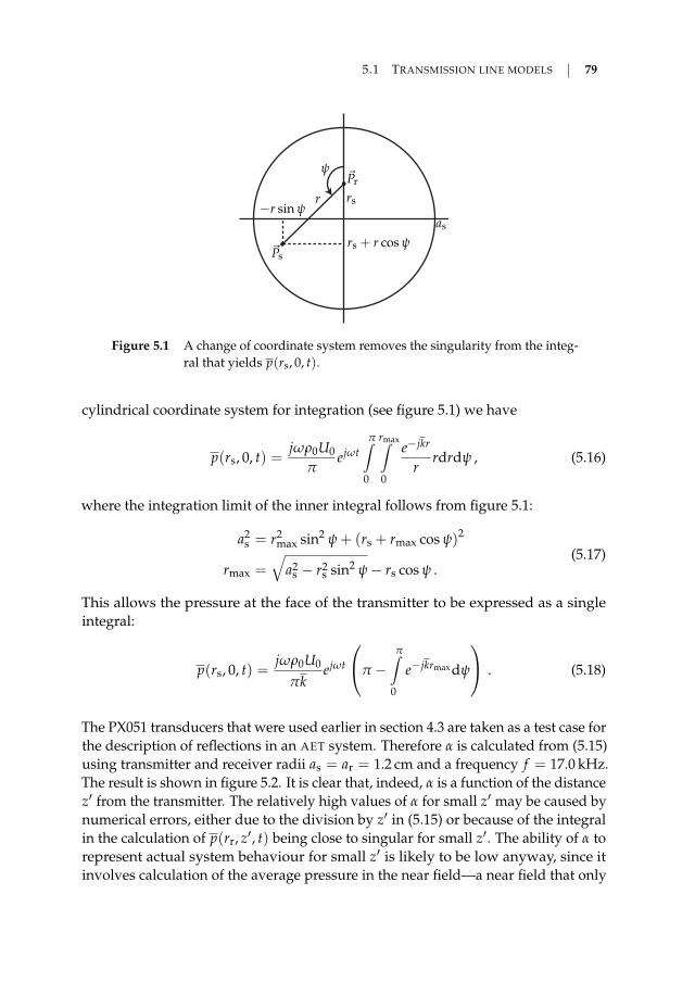
5.1 TRANSMISSION LINE MODELS 79
as
rs
Ps
Prψ
rs + r cos ψ
−r sin ψr
Figure 5.1 A change of coordinate system removes the singularity from the integ-ral that yields p(rs, 0, t).
cylindrical coordinate system for integration (see figure 5.1) we have
p(rs, 0, t) =jωρ0U0
πejωt
π∫0
rmax∫0
e−jkr
rrdrdψ , (5.16)
where the integration limit of the inner integral follows from figure 5.1:
a2s = r2
max sin2 ψ + (rs + rmax cos ψ)2
rmax =√
a2s − r2
s sin2 ψ− rs cos ψ .(5.17)
This allows the pressure at the face of the transmitter to be expressed as a singleintegral:
p(rs, 0, t) =jωρ0U0
πkejωt
π −π∫
0
e−jkrmax dψ
. (5.18)
The PX051 transducers that were used earlier in section 4.3 are taken as a test case forthe description of reflections in an AET system. Therefore α is calculated from (5.15)using transmitter and receiver radii as = ar = 1.2 cm and a frequency f = 17.0 kHz.The result is shown in figure 5.2. It is clear that, indeed, α is a function of the distancez′ from the transmitter. The relatively high values of α for small z′ may be caused bynumerical errors, either due to the division by z′ in (5.15) or because of the integralin the calculation of p(rr, z′, t) being close to singular for small z′. The ability of α torepresent actual system behaviour for small z′ is likely to be low anyway, since itinvolves calculation of the average pressure in the near field—a near field that only
80 CHAPTER 5 REFLECTIONS
α
α
α(m
−1)→
z′ (mm) →
0 20 40 60 80 100 120 140 160 180 2000
5
10
15
20
25
30
35
Figure 5.2 The lumped element attenuation constant α for a transmission linemodel of a rigid circular piston radiator varies as a function of thedistance z′ between the transmitter and the point of observation. A farfield approximation α shows good resemblance for large values of z′.
exist under free radiating conditions. The behaviour will likely be very differentfrom free radiation when the receiver is placed in close proximity to the transmitter.
Figure 5.2 also contains an approximation for α from equation (5.15), where thesource pressure is derived from
pavg(0) =Zrad
πa2s
U0ejωt . (5.19)
The average pressure pavg(z′) at z = z′ is assumed to be equal to the far-field on-
axis pressure from equation (4.18). The far-field approximation of the attenuationconstant is then
α = − 1z′
ln
(ρ0ωπa4
s
2z′∣∣Zrad
∣∣)
, (5.20)
which, according to figure 5.2, is a good approximation for α in the far field of theradiator. Therefore, the numerical integration in (5.15) is not strictly necessary ifonly values of zd are considered that are large in comparison to the transmitter size.
5.1.5 Simulation results
Figure 5.3 shows simulation results of the energy transfer in the transmission lineapproximation of the AET system. The load Za
L was chosen to be real, and the radii ofthe transmitter and the receiver are equal (as = ar = 1.2 cm). The graphs show that
5.1 TRANSMISSION LINE MODELS 81
for ZaL = Za
0 (black line) there indeed are no reflections; the input power does notvary as a function of the distance between the transmitter and the receiver, and theoutput power only decreases with distance due to the losses in the system. The morethe load impedance deviates from this optimal termination, the more reflectionsemerge, and the more pronounced the peaks become. The losses naturally increaseas well as a result of the greater impedance mismatch, which is apparent from theefficiency η in figure 5.3.
Figure 5.4 shows similar results for the same system, but now for various complexload impedances. Again, the input power and output power contain peaks at half-wavelength intervals when Za 6= Za
0 . Note that reflections are even present whenthe absolute value of the load impedance is equal to Za
0 , but it has a small complexphase angle. The efficiency is barely influenced by the reactance of the load.
Although there is still a separation of one half wavelength visible between con-secutive peaks, the peaks for low values of |Za
L| are slightly offset in zd (this isclearly visible in figure 5.5, which shows a detail of the input power). The differencebetween graphs for real and complex load impedance decreases rapidly for an in-crease in |Za
L|. This is in line with (5.14). For |ZaL| ≥ 20Za
0 the graphs are virtuallyindistinguishable.
Comparing these results with the measurements in figure 4.19, one notices immedi-ately that, although the shape of the output power is fairly similar, the shape of theinput power, on the other hand, is very different. Accordingly, sharp peaks appearin the measured efficiency, while the simulated efficiency curve is fairly smooth.
The simulated efficiency contains minima and maxima when dηdzd
= 0, or
dα
dz′
∣∣∣∣zd
= −α(zd)
zd. (5.21)
The absorption coefficient should satisfy this criterion at quarter-wavelength inter-vals to accommodate both maxima and minima in the energy transfer efficiency.Clearly from figure 5.2 it does not.
Note that in both figure 5.3 and 5.4 the resonance peaks (for high load impedance)occur at half wavelength intervals, starting from zd = 1
4 λ. This is due to the choiceof a pressure source at z = 0. The peaks would occur at zd = 1
2 nλ ∀n ∈ Z≥0 shoulda velocity source have been chosen. This is entirely determined by the impedance ofthe transmission line at z′ = 0, since a pressure source delivers maximum power toa low impedance, while a velocity source delivers its maximum power when theimpedance of the transmission line is high.

82 CHAPTER 5 REFLECTIONS
η(−
)→
zd (mm) →
Πa o
ut/
P2 0
(WP
a−
2)→
zd (mm) →
1000Za0
100Za0
20Za0
10Za0
Za0
Πa in/
P2 0
(WP
a−
2)→
zd (mm) →
0 10 20 30 40 50 60 70 80 90 100 110 120
0 10 20 30 40 50 60 70 80 90 100 110 120
0 10 20 30 40 50 60 70 80 90 100 110 120
00.10.20.30.40.50.60.70.80.9
1
10−8
10−7
10−6
10−5
10−4
10−3
10−2
10−6
10−5
10−4
10−3
10−2
10−1
Figure 5.3 Simulation results of the transmission line representation for variousvalues of Za
L show reflections for ZaL 6= Za
0 . The simulation resultswere obtained for as = ar = 1.2 cm and f = 17 kHz. The input powerΠin and output power Πout are normalised to the squared pressureamplitude at z = 0.
5.1 TRANSMISSION LINE MODELS 83
η
(−)→
zd (mm) →
Πa o
ut/
P2 0
(WP
a−
2)→
zd (mm) →
20Za0 ej π
10
20Za0
2Za0 ej π
10
2Za0
Za0ej π
10
Za0
Πa in/
P2 0
(WP
a−
2)→
zd (mm) →
0 10 20 30 40 50 60 70 80 90 100 110 120
0 10 20 30 40 50 60 70 80 90 100 110 120
0 10 20 30 40 50 60 70 80 90 100 110 120
00.10.20.30.40.50.60.70.80.9
1
10−6
10−5
10−4
10−3
10−2
10−5
10−4
10−3
10−2
Figure 5.4 Complex load impedances can add an offset to the location of reflec-tion peaks in the transmission line model, when the load impedancemagnitude is close to the medium’s characteristic impedance.
84 CHAPTER 5 REFLECTIONS
Πa in/
P2 0
(WP
a−
2)→
zd (mm) →2 3 4 5 6 7 8 9 10
10−3
10−2
Figure 5.5 Close up of the input power of the transmission line for various com-plex load impedances. The offset in the location of the peaks is clearlyvisible. The colours represent the same load impedances as in figure5.4: Za
0ej π10 (black), 2Za
0ej π10 (dark grey) and 20Za
0ej π10 (light grey).
5.1.6 Parameter fitting
The purpose of the transmission line model is to describe the effect that reflectionshave on the behaviour of a real acoustic energy transfer system. It is thereforeinteresting to examine the extent to which our simple one-dimensional model agreeswith power measurements of such as system.
Measurements
The model is compared to measurements that were obtained using two PX051 trans-ducers, one of which was mounted on a position controlled linear motor fitted witha linear encoder system. This allowed a positioning accuracy of 1 µm. The distancebetween the transducers was varied in 25 µm increments for the measurements.
The input power to the transmitter was supplied by a Kepco BOP72-6M poweroperational amplifier. It was measured by means of the method described in section4.3.2; A Teledyne LeCroy HDO6034 12-bit oscilloscope measured the power as thecyclic average of the product of the input voltage and current (which was measuredwith a Tektronix TCP312 probe and TCPA300 amplifier). The delay between thevoltage and current probes was compensated using a LeCroy DCS015 deskewcalibration source.
The output power was found from the voltage across the load resistance, measuredfor reasons of accuracy with an Agilent 34401A multimeter. The load resistance wasaccurately measured for this purpose using the same multimeter and a four-wireresistance measurement. Its optimal value proved to be RL = 420 Ω. The electricalcapacitance was not compensated.
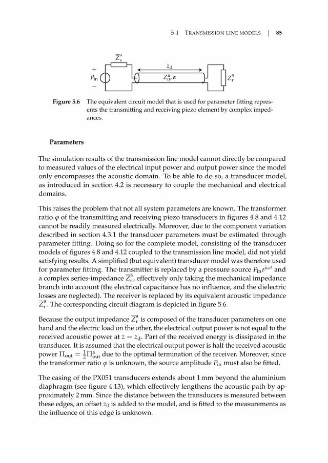
5.1 TRANSMISSION LINE MODELS 85
+
−Pin
Zas
Zar
zd
Za0, α
Figure 5.6 The equivalent circuit model that is used for parameter fitting repres-ents the transmitting and receiving piezo element by complex imped-ances.
Parameters
The simulation results of the transmission line model cannot directly be comparedto measured values of the electrical input power and output power since the modelonly encompasses the acoustic domain. To be able to do so, a transducer model,as introduced in section 4.2 is necessary to couple the mechanical and electricaldomains.
This raises the problem that not all system parameters are known. The transformerratio ϕ of the transmitting and receiving piezo transducers in figures 4.8 and 4.12cannot be readily measured electrically. Moreover, due to the component variationdescribed in section 4.3.1 the transducer parameters must be estimated throughparameter fitting. Doing so for the complete model, consisting of the transducermodels of figures 4.8 and 4.12 coupled to the transmission line model, did not yieldsatisfying results. A simplified (but equivalent) transducer model was therefore usedfor parameter fitting. The transmitter is replaced by a pressure source Pinejωt anda complex series-impedance Za
s , effectively only taking the mechanical impedancebranch into account (the electrical capacitance has no influence, and the dielectriclosses are neglected). The receiver is replaced by its equivalent acoustic impedanceZa
r . The corresponding circuit diagram is depicted in figure 5.6.
Because the output impedance Zar is composed of the transducer parameters on one
hand and the electric load on the other, the electrical output power is not equal to thereceived acoustic power at z = zd. Part of the received energy is dissipated in thetransducer. It is assumed that the electrical output power is half the received acousticpower Πout =
12 Πa
out due to the optimal termination of the receiver. Moreover, sincethe transformer ratio ϕ is unknown, the source amplitude Pin must also be fitted.
The casing of the PX051 transducers extends about 1 mm beyond the aluminiumdiaphragm (see figure 4.13), which effectively lengthens the acoustic path by ap-proximately 2 mm. Since the distance between the transducers is measured betweenthese edges, an offset z0 is added to the model, and is fitted to the measurements asthe influence of this edge is unknown.
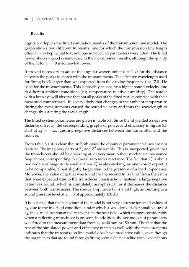
86 CHAPTER 5 REFLECTIONS
Results
Figure 5.7 depicts the fitted simulation results of the transmission line model. Thegraph shows two different fit results: one for which the transmission line lengthoffset z0 was kept equal to 0, and one in which all parameters were fitted. The fittedmodel shows a good resemblance to the measurement results, although the qualityof the fit for z0 = 0 is somewhat lower.
It proved necessary to adjust the angular wavenumber k = 2π/λ for the distancebetween the peaks to match with the measurements. The effective wavelength usedfor fitting is 6 % larger than was expected from the driving frequency f = 17.0 kHzused for the measurements. This is possibly caused by a higher sound velocity dueto different ambient conditions (e.g. temperature, relative humidity). The readerwith a keen eye will observe that not all peaks of the fitted results coincide with theirmeasured counterparts. It is very likely that changes in the ambient temperatureduring the measurements caused the sound velocity and thus the wavelength tochange, thus altering the wavelength.
The fitted system parameters are given in table 5.1. Since the fit yielded a negativedistance offset z0, the corresponding graphs of power and efficiency in figure 5.7start at zd = −z0, ignoring negative distances between the transmitter and thereceiver.
From table 5.1 it is clear that in both cases the obtained parameter values are notrealistic. The imaginary parts of Za
s and Zar are sizable. This is unexpected, given that
the transducers should be operating at, or very near to their mechanical resonancefrequencies, corresponding to a (near) zero series reactance. The fact that Za
r is abouttwo orders of magnitude smaller than Za
s is also striking, as one would expect itto be comparable, albeit slightly larger due to the presence of a load impedance.Moreover, the value of z0 that was found for the second fit is far off from the 2 mmthat were expected due to the transducer construction. Instead, a large negativevalue was found, which is completely non-physical, as it decreases the distancebetween both transducers. The source amplitude Pin is a bit high, amounting to asound pressure level at z = 0 of approximately 138 dB.
It is expected that the behaviour of the model is not very accurate for small values ofzd, due to the free field conditions under which α was derived. For small values ofzd, the virtual location of the receiver is in the near field, which changes considerablywhen a reflecting transducer is present. In addition, the second set of parameterswas fitted to the measurement data from zd = 40 mm to 150 mm. The fact that therest of the simulated power and efficiency match so well with the measurementsindicates that the transmission line model does have predictive value, even thoughthe parameters that are found through fitting seem to be not in line with expectations.
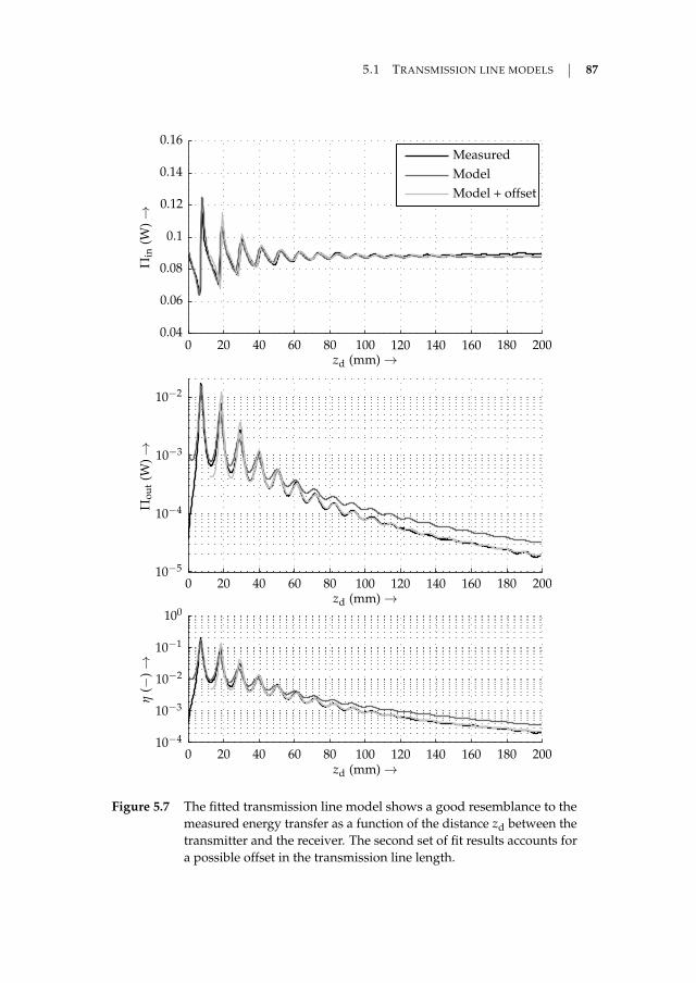
5.1 TRANSMISSION LINE MODELS 87
η
(−)→
zd (mm) →
Πo
ut
(W)→
zd (mm) →
Model + offset
Model
MeasuredΠ
in(W
)→
zd (mm) →
0 20 40 60 80 100 120 140 160 180 200
0 20 40 60 80 100 120 140 160 180 200
0 20 40 60 80 100 120 140 160 180 200
10−4
10−3
10−2
10−1
100
10−5
10−4
10−3
10−2
0.04
0.06
0.08
0.1
0.12
0.14
0.16
Figure 5.7 The fitted transmission line model shows a good resemblance to themeasured energy transfer as a function of the distance zd between thetransmitter and the receiver. The second set of fit results accounts fora possible offset in the transmission line length.

88 CHAPTER 5 REFLECTIONS
Table 5.1 Fitted parameter values of the transmission line model, both with andwithout position offset.
Parameter z0 = 0 z0 6= 0 Unit
Pin 1.68 1.978 kPaZa
s 2.39 + j3.53 3.92 + 4.97 kN s m−3
Zar 62.12− j220.66 41.02− j102.77 N s m−3
z0 0 −12.32 mm
The accuracy of the measurements is high enough for the parameters to be fitted.The maximum measurement error in the output power measurement at its lowestmeasured value of Πout = 19.5 µW is εΠout = 29.1 nW, or 0.15 %. The distance wasvaried in 250 µm increments, in order to capture all peaks adequately. Accordingly,the total measurement comprises 801 measurement points, which is sufficient forparameter fitting.
5.2 Finite element modelling
It is nearly impossible to create an analytical model of an AET system that yieldsclosed form solutions, without resorting to approximations and simplifications. Thisis mostly due to the inherent multiphysical and three-dimensional nature of such asystem. Finite element (FE) analysis seems ideal in this respect, since it is capableof solving the differential equations that govern every domain of physics, couplingthem through boundary conditions. Via subdivision into small elements such amethod is capable of tackling multidimensional problems with considerable ease.
The AET system was modelled using a finite element method in Comsol Multiphysicsin an attempt to create a comprehensive model that describes:
• the coupling between the electrical and mechanical domains through a piezo-electric material
• the structural mechanics governing the behaviour of the piezoelectric patchand the aluminium diaphragm
• the coupling of the transducer to the medium
• the wave propagation through the medium
• and lastly, and most importantly for this chapter: the occurrence of reflectionsat boundaries.

5.2 FINITE ELEMENT MODELLING 89
zr
rdrs2
rs1
rp
hdhp
ca
cb
cc
cb
cb
cd
ce
cf cg
Figure 5.8 The geometry that is used for the finite element analysis is a slightsimplification of the PX051 piezo transducer. The piezoelectric mater-ial is indicated in black, the casing of the transducer in grey and thehatched part is an aluminium diaphragm. The model is axisymmetricaround the dashed line at r = 0 m.
The FE model mainly comprises two piezo transducers placed a distance zd apartwith aligned centres. The transducer model, the geometry of which is shown infigure 5.8, is a simplification of the EMCT SA PX051 piezo transducers that wereused for earlier experiments. The values of the parameters in figure 5.8 are given intable 5.2.
The casing of a transducer, indicated in grey in figure 5.8, is assumed to be suffi-ciently rigid to neglect its vibrations. Therefore it is modelled as an acoustic hardwall, which is a perfectly reflecting boundary condition where the normal particlevelocity vanishes. In the model, the transducers are placed in a spherical air domainsurrounded by a so-called perfect matching layer, which is a coordinate transforma-tion simulating an infinite air domain. This prevents reflections from the domainboundaries. The model does not include sound absorption in the air or mechanicallosses in the transducers.
The electrical contacts of the piezoelectric material are located on its top and bottom.Logically, these are the same contacts that were used for polarisation of the material.Hence the piezoelectric material is assumed to be polarised in the z-direction. Theexact type of piezoelectric ceramic that is used in the transducers is unknown.Simulations of the maximum energy transfer efficiency were performed for variousPZT (lead zirconate titanate) grades. Table 5.3 lists the efficiency of the AET system atthe first peak in the transfer efficiency, as well as the distance between the transducerszd and frequency f at which this peak occurs. The table indicates that, although the
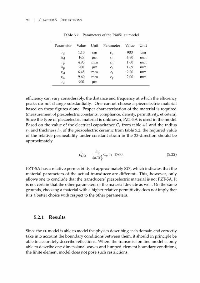
90 CHAPTER 5 REFLECTIONS
Table 5.2 Parameters of the PX051 FE model
Parameter Value Unit Parameter Value Unit
rd 1.10 cm cb 900 µmhd 165 µm cc 4.80 mmrp 4.95 mm cd 1.60 mmhp 200 µm ce 1.69 mmrs1 6.45 mm cf 2.20 mmrs2 9.60 mm cg 2.00 mmca 900 µm
efficiency can vary considerably, the distance and frequency at which the efficiencypeaks do not change substantially. One cannot choose a piezoelectric materialbased on these figures alone. Proper characterisation of the material is required(measurement of piezoelectric constants, compliance, density, permittivity, et cetera).Since the type of piezoelectric material is unknown, PZT-5A is used in the model.Based on the value of the electrical capacitance Ce from table 4.1 and the radiusrp and thickness hp of the piezoelectric ceramic from table 5.2, the required valueof the relative permeability under constant strain in the 33-direction should beapproximately
εSr,33 =
hp
ε0πr2p
Ce ≈ 1760. (5.22)
PZT-5A has a relative permeability of approximately 827, which indicates that thematerial parameters of the actual transducer are different. This, however, onlyallows one to conclude that the transducers’ piezoelectric material is not PZT-5A. Itis not certain that the other parameters of the material deviate as well. On the samegrounds, choosing a material with a higher relative permittivity does not imply thatit is a better choice with respect to the other parameters.
5.2.1 Results
Since the FE model is able to model the physics describing each domain and correctlytake into account the boundary conditions between them, it should in principle beable to accurately describe reflections. Where the transmission line model is onlyable to describe one-dimensional waves and lumped-element boundary conditions,the finite element model does not pose such restrictions.
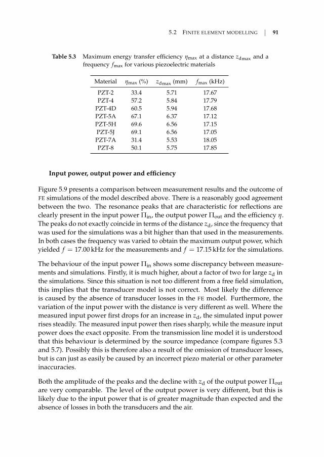
5.2 FINITE ELEMENT MODELLING 91
Table 5.3 Maximum energy transfer efficiency ηmax at a distance zdmax and afrequency fmax for various piezoelectric materials
Material ηmax (%) zdmax (mm) fmax (kHz)
PZT-2 33.4 5.71 17.67PZT-4 57.2 5.84 17.79
PZT-4D 60.5 5.94 17.68PZT-5A 67.1 6.37 17.12PZT-5H 69.6 6.56 17.15PZT-5J 69.1 6.56 17.05PZT-7A 31.4 5.53 18.05PZT-8 50.1 5.75 17.85
Input power, output power and efficiency
Figure 5.9 presents a comparison between measurement results and the outcome ofFE simulations of the model described above. There is a reasonably good agreementbetween the two. The resonance peaks that are characteristic for reflections areclearly present in the input power Πin, the output power Πout and the efficiency η.The peaks do not exactly coincide in terms of the distance zd, since the frequency thatwas used for the simulations was a bit higher than that used in the measurements.In both cases the frequency was varied to obtain the maximum output power, whichyielded f = 17.00 kHz for the measurements and f = 17.15 kHz for the simulations.
The behaviour of the input power Πin shows some discrepancy between measure-ments and simulations. Firstly, it is much higher, about a factor of two for large zd inthe simulations. Since this situation is not too different from a free field simulation,this implies that the transducer model is not correct. Most likely the differenceis caused by the absence of transducer losses in the FE model. Furthermore, thevariation of the input power with the distance is very different as well. Where themeasured input power first drops for an increase in zd, the simulated input powerrises steadily. The measured input power then rises sharply, while the measure inputpower does the exact opposite. From the transmission line model it is understoodthat this behaviour is determined by the source impedance (compare figures 5.3and 5.7). Possibly this is therefore also a result of the omission of transducer losses,but is can just as easily be caused by an incorrect piezo material or other parameterinaccuracies.
Both the amplitude of the peaks and the decline with zd of the output power Πoutare very comparable. The level of the output power is very different, but this islikely due to the input power that is of greater magnitude than expected and theabsence of losses in both the transducers and the air.

92 CHAPTER 5 REFLECTIONS
η
(−)→
zd (mm) →
Πo
ut
(W)→
zd (mm) →
FE model
MeasuredΠ
in(W
)→
zd (mm) →
0 20 40 60 80 100 120 140 160 180 200
0 20 40 60 80 100 120 140 160 180 200
0 20 40 60 80 100 120 140 160 180 200
10−4
10−3
10−2
10−1
100
10−5
10−4
10−3
10−2
10−1
100
0
0.1
0.2
0.3
0.4
0.5
0.6
0.7
Figure 5.9 The energy transfer efficiency η was calculated by means of FE analysisas a function of the distance zd between the transmitting and receivingpiezo elements. A driving frequency of f = 17.152 kHz was used forthe simulations.

5.2 FINITE ELEMENT MODELLING 93
Lastly the efficiency is again comparable, although the effect of the reflections isnot as pronounced in the FE results as it is in the measurements. This is put downchiefly to the discrepancy in the input power, considering the similarity in Πout. Theefficiency is approximately a factor ten higher than expected. The absence of lossesin the model naturally boosts the efficiency. Furthermore, as already indicated bytable 5.3, a wrong choice of piezoelectric material can lead to a large deviation inefficiency.
Pressure amplitude
The reflections cause distinct maxima and minima in the energy transfer and itsefficiency. It is interesting to examine what these maxima and minima mean in termsof the pressure amplitude in the r, z-domain. Our finite element model is a usefultool in this regard, since it calculates this pressure.
There are two ways of approaching the energy transfer; one could either opt to lookat the maximum output power, or the maximum efficiency. These two cases donot necessarily coincide, and in practice occur for slightly different frequencies anddistances. Both situations will be considered here.
A pattern search algorithm [46] was used for finding the maximum output powerand efficiency to prevent false maximum detection due to the numerical inaccuracyof the solver. The model predicts the maximum output power to be produced at adistance zd = 5.557 mm and a frequency f = 17.152 kHz. The first minimum of theoutput power at the same frequency was found at zd = 11.1 mm. Analogously, themaximum efficiency was found for a distance zd = 6.373 mm and f = 17.123 kHz.The first minimum of the efficiency at the same frequency occurred at zd = 12.1 mm.The precision of zd at the minima is lower due to relatively higher noise from the FE
solver.
Figure 5.10 shows the FE simulation results of the pressure amplitude in thesefour situations. The standing waves that originate due to the reflections fromboth transducers are clearly visible as alternating amplitude maxima and minimain the z direction. The pressure amplitude distribution is very different whenlooking at the situation where we have maximum output power (figure 5.10a) ormaximum efficiency (figure 5.10c). The pressure amplitude immediately in frontof the diaphragm of the receiver (top transducer) is about a factor two higher thanin the case of maximum efficiency, naturally leading to a higher output power.Unfortunately, figure 5.10a also shows that a large part of the power radiates awayfrom the back of the transmitter. Figure 5.10c indeed shows a situation where theefficiency will be much higher, as the pressure amplitude is high in front of bothtransducers, implying that the transmitter delivers most of its energy to the medium

94 CHAPTER 5 REFLECTIONS
at the front, and the receiver absorbs much of this energy. This figure shows verywell how reflections, and the standing waves that ensue, cause the impedance ofthe medium to increase, and the matching of the transducer with the medium toimprove.
The pressure amplitude distribution in case of minimum output power (figure5.10b) and minimum efficiency (figure 5.10d) are virtually indistinguishable. Themost important observation to be made from the two figures is that the pressureamplitude at the diaphragm of the receiver is negligible, and therefore the outputpower is as well. The transmitter still delivers its energy to the medium, both at thefront and the back of the diaphragm.
5.2.2 Parameter sensitivity
Table 5.3 already indicated that the performance of the system heavily depends onthe material parameters. The maximum of the simulated efficiency of the systemlies between 33 % and 70 %, depending on the choice of PZT-grade. The material notonly influences the maximum output power and efficiency, but also the resonancefrequency at which these occur. This change in efficiency offers great opportunitiesto increase the energy transfer efficiency, by choosing the right materials for theconstruction of the transducers.
If the simulation results can be altered to such a large extent by changing one materialfor another, the question arises how the results are influenced by the model’s otherparameters, such as the dimensions listed in table 5.2, or the material propertiesof the diaphragm and the piezoelectric ceramic. Quantitative information aboutthe influence of model parameters can be obtained from a sensitivity analysis. Thepurpose of such an analysis is twofold; it gives information on how parameterdeviation influences the outcome of the model, in other words: how accuratelyparameters should be known to be able to construct an accurate model, while, onthe other hand, if performance improvement is the main topic of interest, it indicateswhich parameters will change the system’s output most.
The finite element model was used to investigate the sensitivity of the system toparameter changes. The choice of output variable on the basis of which the sensitivityanalysis is to be performed is an important one. The most useful choice for AET is theoutput power. Unfortunately it depends heavily on the exact location of the receiverand the driving frequency because of the reflections. For a fair comparison one willhave to look at the change in the maximum output power Πout,max for a change in aparameter. The distance zdmax and frequency fmax at which the maximum outputpower occurs and their change are also of interest.
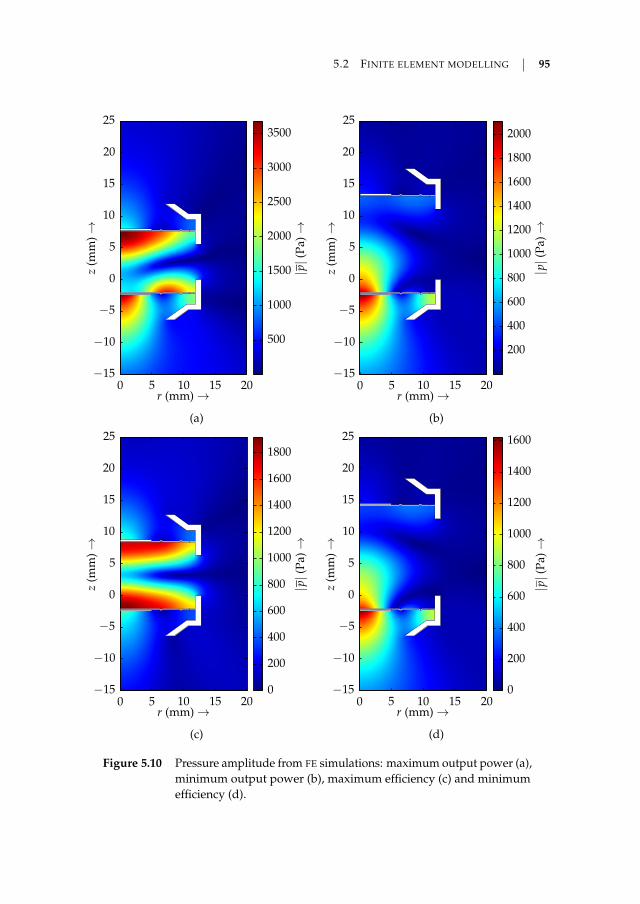
5.2 FINITE ELEMENT MODELLING 95
|p|
(Pa)→
z(m
m)→
r (mm) →0 5 10 15 20
500
1000
1500
2000
2500
3000
3500
−15
−10
−5
0
5
10
15
20
25
(a)
|p|
(Pa)→
z(m
m)→
r (mm) →0 5 10 15 20
200
400
600
800
1000
1200
1400
1600
1800
2000
−15
−10
−5
0
5
10
15
20
25
(b)
|p|
(Pa)→
z(m
m)→
r (mm) →0 5 10 15 20
0
200
400
600
800
1000
1200
1400
1600
1800
−15
−10
−5
0
5
10
15
20
25
(c)
|p|
(Pa)→
z(m
m)→
r (mm) →0 5 10 15 20
0
200
400
600
800
1000
1200
1400
1600
−15
−10
−5
0
5
10
15
20
25
(d)
Figure 5.10 Pressure amplitude from FE simulations: maximum output power (a),minimum output power (b), maximum efficiency (c) and minimumefficiency (d).

96 CHAPTER 5 REFLECTIONS
The sensitivity analysis was carried out for all geometric parameters in table 5.2, theload resistance RL, the piezoelectric stress constant e in the 31, 33 and 15 directions,the elasticity matrix cE (on account of practical reasons the whole matrix is scaledas cE = λcE
0 , and only λ is varied), the relative permittivity εSr,33 of the PZT material,
its density ρPZT, the Young’s modulus EAl of the diaphragm, its density ρAl and thePoisson’s ratio νAl.
Each parameter p was varied by a small increment σp0 from its default value p0,after which the new maximum output power Πmax,out(p) was sought by means of apattern search algorithm:
Πout,max(p) = maxzd, f
Πout (5.23a)
(zdmax(p) , fmax(p)) = arg maxzd, f
Πout (5.23b)
From the variation in the maximum output power one can determine the relativesensitivity of a variable y for a change in parameter p as
∂y∂p
p0
y0, ∀y ∈ Πout,max, zdmax, fmax (5.24)
To reduce the influence of numerical errors from the simulation, the partial derivativeis calculated by means of a five-point Lagrange’s formula [5]. The relative sensitivityis then
∂y∂p
p0
y0=
y((1− 2σ) p0)− y((1 + 2σ) p0)
12σy0− 2
y((1− σ) p0)− y((1 + σ) p0)
3σy0(5.25)
This sensitivity analysis was performed for σ = 1 · 10−3.
The relative sensitivities of the output power to changes in the parameters are listedin table 5.4. The output power is affected most by the radius of the aluminium dia-phragm rd. Fortunately, it is easy to measure, and is therefore unlikely to introducemodelling errors. Other important parameters are the radius and thickness of thepiezoelectric patch, the latter being somewhat more difficult to accurately measure.Furthermore the output power is sensitive to changes in the location rs1 of the firstnotch in the diaphragm, and a number of dimensions of the casing. Surprisingly,the material properties of the diaphragm have little influence on the output power.The material properties of the piezoelectric ceramic seem to influence it much more.Especially the elasticity of the material and the piezoelectric stress constant in the33-direction affect the output power.
Not only the efficiency is influenced by the variation of parameters, but also theposition and the frequency at which the efficiency maxima occur are subject tochange. This change is reflected by ∂zdmax
∂pp0
zdmax0and ∂ fmax
∂pp0
fmax0. It is striking that the
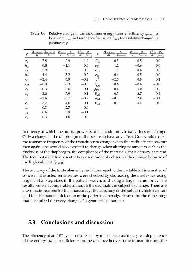
5.3 CONCLUSIONS AND DISCUSSION 97
Table 5.4 Relative change in the maximum energy transfer efficiency ηmax, itslocation zdmax and resonance frequency fmax for a relative change in aparameter p
p ∂Πout,max∂p
Πout,max0p0
∂zdmax∂p
p0zdmax0
∂ fmax∂p
p0fmax0
p ∂Πout,max∂p
p0Πout,max0
∂zdmax∂p
p0zdmax0
∂ fmax∂p
p0fmax0
rd −7.8 2.9 −1.9 RL 0.5 −0.5 0.0hd 0.8 −1.1 0.6 e31 1.2 −0.6 0.0rp 2.9 0.1 −0.0 e33 1.9 −0.6 0.0hp −4.4 5.2 0.2 e15 0.4 −0.5 0.0rs1 −2.4 6.9 −0.2 cE −2.5 0.8 0.1rs2 −0.9 6.3 −0.0 εS
r,33 0.6 −0.6 −0.0ca −0.3 3.0 −0.1 ρPZT 0.4 5.0 −0.2cb −2.0 5.9 −0.1 EAl 0.5 3.7 0.2cc −3.6 6.7 −0.2 ρAl −0.2 2.9 −0.4cd −3.7 4.6 −0.1 νAl 0.1 3.4 0.0ce 0.3 2.7 −0.0cf 0.6 3.9 −0.1cg 0.3 1.6 −0.0
frequency at which the output power is at its maximum virtually does not change.Only a change in the diaphragm radius seems to have any effect. One would expectthe resonance frequency of the transducer to change when this radius increases, butthen again, one would also expect it to change when altering parameters such as thethickness of the diaphragm, the compliance of the materials, their density, et cetera.The fact that a relative sensitivity is used probably obscures this change because ofthe high value of fmax,0.
The accuracy of the finite element simulations used to derive table 5.4 is a matter ofconcern. The listed sensitivities were checked by decreasing the mesh size, usinglarger initial step sizes in the pattern search, and using a larger value for σ. Theresults were all comparable, although the decimals are subject to change. There area two main reasons for this inaccuracy: the accuracy of the solver (which also canlead to false maxima detection of the pattern search algorithm) and the remeshingthat is required for every change of a geometric parameter.
5.3 Conclusions and discussion
The efficiency of an AET system is affected by reflections, causing a great dependenceof the energy transfer efficiency on the distance between the transmitter and the

98 CHAPTER 5 REFLECTIONS
receiver. The peaks in the output power and efficiency, which are a consequence ofthe reflections, restrict the free placement of the receiver if a high energy transferefficiency and output power are desired.
One possible approach to dealing with reflections is to design a system were they donot play a large role. An example is the system by Shahab et al. [109,111], that uses areceiver that is small in comparison to the wavelength, and a spherically radiatingsource. The disadvantages of such a system are the low received power and thelow transfer efficiency as a consequence of these design choices. It does, however,greatly simplify the modelling of the system. In contrast, in this chapter effort wasmade to model reflections, since they prove a key aspect of an AET system where ahigh directionality is used in combination with a receiver of dimensions comparableto or larger than the wavelength.
This chapter outlines two models that describe the reflections that occur in an AET
system where the transducers are imperfectly matched to the medium between them.The first model, based on transmission line theory, is a completely analytical model,based on one-dimensional wave propagation, where the combined diffraction andabsorption losses are accounted for by means of a lumped attenuation constant.This constant is derived from a vibrating piston model. The second model is afinite element model of the system where the electrical, mechanical and acousticaldomains are described and linked to each other through appropriate boundaryconditions.
The transmission line model is able to model reflections, but depends heavily on agood transducer model. It is possible to approach measured values of the input andoutput power to a good degree by means of this model, but the resulting transducerparameters are unrealistic. Without a properly validated transducer model, of whichall the parameters are a priori known, it is impossible to say whether the good qualityof the fitted model’s simulation results is a consequence of the correctness of thetransmission line model, or that all errors in the model are smoothed away by theparameter fitting and end up in the transducer model parameters. Measurementsof acoustic variables (pressures and velocities) would allow a direct comparison tovalues from the transmission line model and can therefore be used to validate themodel, in the absence of sufficient knowledge of the transducer model.
Notwithstanding this consideration, the transmission line models seems to be ableto describe the reflections that occur in a typical AET system quite well. Hence, itwould seem that the transmission line model is at the very least a step in the rightdirection.
The transmission line model predicts that, as one would expect, the resonance peaksas a function of the distance between the two transducers completely disappearwhen the receiving transducer presents an impedance to the medium that is exactly

5.3 CONCLUSIONS AND DISCUSSION 99
equal to the medium’s characteristic impedance.
Although finite element analysis seems to be able to describe reflections and thegeneral behaviour of an acoustic energy transfer system, it is far from the holygrail in modelling. The FE model is able to model reflections, but the predictedoutput power is an order of magnitude too high. The variation of the input powerwith the distance between the two transducers is considerably different from themeasurements. This suggests that the transducer is likely incorrectly modelled.This can be caused by parameter deviation, an incorrectly modelled geometry, theabsence of losses, unmodelled nonlinear behaviour, or a combination of any of these.
A sensitivity analysis indicates that a change of piezoelectric material can have agreat impact on the energy transfer efficiency. Other important parameters are thediaphragm radius, the piezoelectric disc dimensions and the dimensions of theplastic casing. It will therefore require much effort and proper characterisation ofall system, geometry and material parameters to arrive at a model that is able todescribe the quantities of interest to an adequate level of accuracy.
The transmission line model predicts that a perfect termination of the acoustic pathleads to a total absence of reflections. The impedance of the receiving transducermust therefore be adapted to the medium’s characteristic impedance. Impedancematching of transducers to a medium can be achieved in a number of ways. Amethod that is often applied for piezoelectric transducers is the use of quarter-wavelength matching layers [17, 41, 64]. As the name implies, these are layers ofa thickness corresponding to a quarter of a wavelength in the material, that arebonded to the radiating face of the transducer. The material itself is chosen to havea characteristic impedance between the transducer’s and medium’s characteristicimpedances. Often multiple consecutive layers are used for an even better adaptation[41], each one successively decreasing in characteristic impedance from that of thetransducer to the loading medium. Matching layers are used less frequently in air,because of the need for very low acoustic impedance materials, which are generallyextremely lossy and ill suited for use with piezo transducers due to difficulties inbonding them to the transducer surface, in tuning them to the transducer’s resonancefrequency and their porosity [6, 7, 132]
Acoustic horns (as applied for example in horn drivers, sirens and megaphones)[15,20,44,61,62,128] can be used to convert the large reactive radiation impedance ofa small transducer into a larger real impedance, and can convert a small transducervelocity to a larger particle velocity in the horn. Moreover, a horn gives control overthe directivity of the transducer, which is another desirable feature in an AET system.
A final often applied method of impedance matching is the enlargement of theradiating surface of the transducer, commonly accomplished with membranes ordiaphragms, such as the cone in a traditional voice coil loudspeaker [15, 20], or

100 CHAPTER 5 REFLECTIONS
trough the use of multiple direct radiators in parallel.
The last two methods of impedance adaptation will be examined in more detail in thenext two chapters. Chapter 6 deals with the use of horns in AET systems operatingin air. Chapter 7 investigates the influence of an increased radiation surface on theenergy transfer.
CH
AP
TE
R
6 Horns
REFLECTIONS are caused by an impedance mismatch at the side of the receiver,basically no differently from a poorly terminated transmission line, as wasexplained in the previous chapter. They are undesirable, in the sense that
they introduce maxima and minima into the energy transfer and the efficiency, andthereby limit the placement of the receiver to distinct locations where the energytransfer peaks. A receiver that presents a perfect impedance match to the mediumis able to absorb all the energy contained in the incident wave, without generatingreflections (see figure 5.3). But it is not only an impedance mismatch at the receivingend that affects the energy transfer. The impedance mismatch that exists betweenthe transmitting transducer and the medium limits the power that can be transferred.A perfectly matched transmitter transfers the maximum amount of energy to themedium.
Impedance adaptation for transducers in essence amounts to conversion of either thepressure or the particle velocity at the radiating face of the transducer, or both. As aresult the transducer experiences a better match with its own impedance. Section5.3 already mentioned a number of methods with which this can be accomplished.This chapter specifically addresses the use of horns for this purpose. It describes thedesign and optimisation of horns for AET that employ internal reflections to boostthe throat impedance.
This chapter is based on [99] and [100].
101
102 CHAPTER 6 HORNS
6.1 Waveguides
Let us first look at what a horn actually is. In essence it is a structure that limits thespreading of a wave. It is therefore a waveguide; a structure that guides the soundwave as it propagates along a path. In its simplest form, a waveguide is a pipe of aconstant cross section. This type of wave guide was already discussed in section 5.1,where it was used to model reflections analytically.
Let us apply the coordinate transformation mentioned in footnote 1 on page 75,setting z = −l, and terminating the waveguide with an impedance Za
(0) = p(0)/u(0)
at z = 0. A positive l corresponds to a location a distance l to the left of z = 0.Equations (5.1) and (5.2) can be combined to find the impedance Za
(l) as
Za(l) = Za
0Za
(0) + jZa0 tan(kl)
Za0 + jZa
(0) tan(kl), (6.1)
which is a well-known standard expression1. Losses are neglected in this case, hencek is real.
If the cross-sectional area of the waveguide changes at z = 0 from A1 to A2, suchas depicted in figure 6.1, the situation becomes somewhat different. We will makethe assumption here that the waves inside the waveguide are always plane waves.Imagine that we have a pressure p(0−) and a particle velocity u(0−) immediatelyleft of the discontinuity and a pressure and particle velocity p(0+) and u(0+) tothe right. The pressure should be continuous across the boundary, implying thatp(0−) = p(0+). Continuity relations also dictate that the mass flow (and hencethe volume flow) be constant across the discontinuity, or A1u(0−) = A2u(0+).Therefore the impedances directly left and right of the discontinuity are related by
Za(0−) = A1
A2Za(0+) . (6.2)
A step change in the diameter of a pipe can therefore be used to increase the imped-ance seen by a transducer or the medium (or decrease it when desired).
Now, let us consider the impedance a distance l away from the discontinuity. Itfollows from the combination of (6.1) and (6.2), and is equal to
Za(l) = Za
0A1Za+
+ jA2Za0 tan(kl)
A2Za0 + jA1Za+ tan(kl)
, (6.3)
1On a side node, equation (6.1) explains how quarter-wavelength matching layers can be used forimpedance adaptation. For a length corresponding to a quarter-wavelength kl = 1
2 π, the impedancebecomes Za
(l) = Za0
2/Za(0) and can thus be tuned by a proper choice of Za
0 . The only other length thatyields a real impedance is l = 1
2 λ, resulting in the not overly useful Za(l) = Za
(0).

6.2 EXPONENTIAL HORNS 103
A1 A2
Figure 6.1 A waveguide with a change in cross-sectional area at z = 0.
using the shorthand notation Za+= Za
(0+).
6.2 Exponential horns
If the cross-sectional area of a pipe changes continuously, instead of abruptly as infigure 6.1, and it increases monotonically, such a pipe is normally referred to as ahorn [69]. Based on the force and mass balance in a horn, one can derive a differentialequation that describes the pressure in it. This equation, known as Webster’s hornequation [69, 128], is given by
∂2 p∂z2 +
d ln(A)
dz∂ p∂z
=1c2
∂2 p∂t2 . (6.4)
It is derived under the assumption that the waves in the horn are (nearly) plane,which is only possible as long as the surface area A changes very slowly as a functionof z.
Let us now look at a horn of which the surface area varies exponentially as
A(z) = A0emz , (6.5)
with m the flare constant of the horn. The differential equation (6.4) for the pressurewaves in this horn can then be written as
∂2 p∂z2 + m
∂ p∂z
=1c2
∂2 p∂t2 . (6.6)
Substitution of a plane wave solution p(z, t) = Peσzejωt gives
σ2 + mσ + k2 = 0 , (6.7)
where the angular wave number k = ω/c is again introduced. This equation has thesolutions σ = −α± jβ, with α = 1
2 m and β =√
k2 − α2. Note that a travelling wavesolution only exists for β ∈ R, or ω > ωc =
12 mc. The horn therefore has a distinct
cutoff frequency and acts as a high pass filter.
104 CHAPTER 6 HORNS
6.2.1 Infinite horns
If we make the assumption that the horn is infinitely long, there is no interface fromwhich reflections can occur, and hence there will only be a wave travelling in thepositive z-direction. This wave corresponds to the solution σ = jβ− α, or
p(z, t) = Pe−12 mzej(ωt−βz) . (6.8)
The factor e−12 mz is the dilution [69] that accounts for the waves having to cover an
area that increases with the spatial coordinate z.
The particle velocity u(z, t) in the horn can be obtained from the solution of thepressure (6.8) by means of equation (3.19), which can be written in this case as
u = − 1jρ0ω
∂ p∂z
=p
Za0
(√1−
(ωc
ω
)2− j
ωc
ω
).
(6.9)
The ratio between the pressure and the particle velocity gives us the effective charac-teristic impedance that the wave experiences inside the horn. It is equal to
Za0,h =
pu
= Za0
(√1−
(ωc
ω
)2+ j
ωc
ω
).
(6.10)
Note that this impedance does not depend on the z-coordinate and thus is constantthroughout the horn. Therefore it is effectively the impedance that a source placed atthe the throat (the narrow end) of the horn will have to work against. The radiationresistance of this transducer, determining its radiated power, hence is equal to
Rrad,h = A0 Re(
Za0,h
)= A0Za
0
√1−
(ωc
ω
)2.
(6.11)
Comparing this radiation impedance to that of a circular piston, given by equation(4.12), one can see in figure 6.2 that the low frequency radiation of a plane pistonis greatly improved by application of a horn. This is a great advantage for audioapplications, as is the flat frequency response of the horn in comparison to the pistonradiator. Unfortunately, acoustic energy transfer does not really benefit from either,
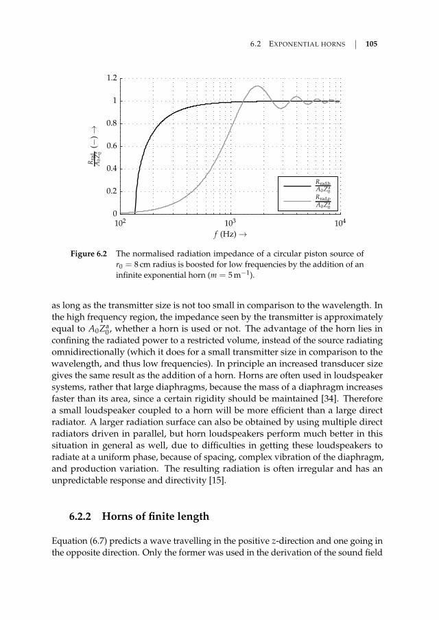
6.2 EXPONENTIAL HORNS 105
Rrad,p
A0Za0
Rrad,h
A0 Za0
Rra
dA
0Z
a 0(−
)→
f (Hz) →
102 103 1040
0.2
0.4
0.6
0.8
1
1.2
Figure 6.2 The normalised radiation impedance of a circular piston source ofr0 = 8 cm radius is boosted for low frequencies by the addition of aninfinite exponential horn (m = 5 m−1).
as long as the transmitter size is not too small in comparison to the wavelength. Inthe high frequency region, the impedance seen by the transmitter is approximatelyequal to A0Za
0 , whether a horn is used or not. The advantage of the horn lies inconfining the radiated power to a restricted volume, instead of the source radiatingomnidirectionally (which it does for a small transmitter size in comparison to thewavelength, and thus low frequencies). In principle an increased transducer sizegives the same result as the addition of a horn. Horns are often used in loudspeakersystems, rather that large diaphragms, because the mass of a diaphragm increasesfaster than its area, since a certain rigidity should be maintained [34]. Thereforea small loudspeaker coupled to a horn will be more efficient than a large directradiator. A larger radiation surface can also be obtained by using multiple directradiators driven in parallel, but horn loudspeakers perform much better in thissituation in general as well, due to difficulties in getting these loudspeakers toradiate at a uniform phase, because of spacing, complex vibration of the diaphragm,and production variation. The resulting radiation is often irregular and has anunpredictable response and directivity [15].
6.2.2 Horns of finite length
Equation (6.7) predicts a wave travelling in the positive z-direction and one going inthe opposite direction. Only the former was used in the derivation of the sound field
106 CHAPTER 6 HORNS
in the infinite horn, since reflections can never occur in it. In practice, however, a hornwill always have a finite length. An infinite horn can at best only be approximated.The true pressure field will therefore be a superposition of both solutions.
A complete derivation of the pressure field inside a horn of finite length will not begiven in this section. Instead the resulting throat impedance will merely be given. Itis equal to (see [21, 120]):
Zat = Za
0jZa
0 sin(βl) + Zam cos(βl + θ)
jZam sin(βl) + Za
0 cos(βl − θ), (6.12)
with tan θ = α/β. Since we are now dealing with a horn of finite length l, the throatimpedance Za
t depends on the impedance Zam at the mouth of the horn (the wide
end). The form of (6.12) is reminiscent of the equation describing the impedance ofa transmission line (6.1), which a horn of course is in a certain sense.
The value of the mouth impedance Zam is normally approximated in literature by that
of a baffled circular piston source (see equation (4.12)). This is an exact representationas long as the waves arriving at the mouth of the horn are plane waves and the hornmouth is embedded in a baffle. In practice it will therefore only be an approximation.Note that Za
m is an acoustic impedance, instead of a mechanical impedance. Theradiation impedance from (4.12) should therefore be divided by the mouth surfacearea.
Figure 6.3 depicts the throat impedance from equation (6.12) for a horn mouth radiusof 10 cm, 20 cm, 30 cm and that of an infinite horn. The throat radius is 8 cm in allfour situations, and the horn flare constant is m = 5 m−1, just as in figure 6.2. Thegraphs show that the longer the horn is, the more its throat impedance approachesthat of an infinite exponential horn. The horn impedance now peaks at certainresonance frequencies, as a consequence of the horn’s finite length. These peakssurpass the Za
0-level, which can at maximum be attained by means of an infinitehorn, and which is approximately the maximum radiation resistance of a planepiston. A finite horn is therefore capable of boosting the impedance seen by thetransducer.
The asymmetric oscillations that are visible in the throat impedance (for examplearound f = 2 kHz for rm = 10 cm) are caused by the oscillatory behaviour of theradiation impedance of a circular piston, (see figure 4.3 or 6.2). Furthermore, thefirst peak of the impedance is significantly higher than the others for small hornmouth sizes. This is a direct result of the low radiation impedance of the mouth forsmall sizes and low frequencies (cf. figure 4.3), having large reflections as a result,comparable to a large impedance mismatch in a transmission line.
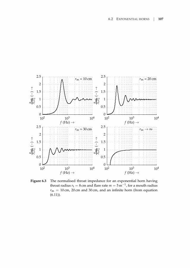
6.2 EXPONENTIAL HORNS 107
Rra
d
A0Z
a 0
(−)→
f (Hz) →
Rra
d
A0Z
a 0
(−)→
f (Hz) →
Rra
d
A0Z
a 0
(−)→
f (Hz) →
Rra
d
A0Z
a 0
(−)→
f (Hz) →
rm → ∞rm = 30 cm
rm = 20 cmrm = 10 cm
102 103 104102 103 104
102 103 104102 103 104
0
0.5
1
1.5
2
2.5
0
0.5
1
1.5
2
2.5
0
0.5
1
1.5
2
2.5
0
0.5
1
1.5
2
2.5
Figure 6.3 The normalised throat impedance for an exponential horn havingthroat radius rt = 8 cm and flare rate m = 5 m−1, for a mouth radiusrm = 10 cm, 20 cm and 30 cm, and an infinite horn (from equation(6.11)).
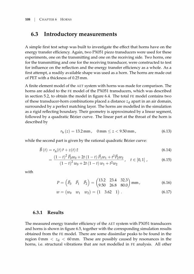
108 CHAPTER 6 HORNS
6.3 Introductory measurements
A simple first test setup was built to investigate the effect that horns have on theenergy transfer efficiency. Again, two PX051 piezo transducers were used for theseexperiments, one on the transmitting and one on the receiving side. Two horns, onefor the transmitting and one for the receiving transducer, were constructed to testfor influence on the reflection and the energy transfer efficiency as a whole. As afirst attempt, a readily available shape was used as a horn. The horns are made outof PET with a thickness of 0.25 mm.
A finite element model of the AET system with horns was made for comparison. Thehorns are added to the FE model of the PX051 transducers, which was describedin section 5.2, to obtain the model in figure 6.4. The total FE model contains twoof these transducer-horn combinations placed a distance zd apart in an air domain,surrounded by a perfect matching layer. The horns are modelled in the simulationas a rigid reflecting boundary. Their geometry is approximated by a linear segment,followed by a quadratic Bézier curve. The linear part at the throat of the horn isdescribed by
rh (z) = 13.2 mm , 0 mm ≤ z < 9.50 mm , (6.13)
while the second part is given by the rational quadratic Bézier curve:
~B (t) = rh(t) r + z(t) z (6.14)
=(1− t)2 ~P0w0 + 2t (1− t) ~P1w1 + t2~P2w2
(1− t)2 w0 + 2t (1− t)w1 + t2w2, t ∈ [0, 1] , (6.15)
with
P =(~P0 ~P1 ~P2
)=
(13.2 23.4 32.39.50 26.8 80.0
)mm , (6.16)
w =(w0 w1 w2
)=(1 3.62 1
). (6.17)
6.3.1 Results
The measured energy transfer efficiency of the AET system with PX051 transducersand horns is shown in figure 6.5, together with the corresponding simulation resultsobtained from the FE model. There are some dissimilar peaks to be found in theregion 0 mm < zd < 60 mm. These are possibly caused by resonances in thehorns, i.e. structural vibrations that are not modelled in FE analysis. All other

6.3 INTRODUCTORY MEASUREMENTS 109
zr
rh(z)
lh
Figure 6.4 The radius rh (z) of the horns that are used in the measurementsis described in the FE model by means of Bézier curves. They aremodelled as ideal hard acoustic boundaries.
characteristics of the simulated and experimentally determined efficiency are verysimilar. The relative amplitude of the peaks in comparison to their mean is equalfrom approximately zd = 100 mm onwards, just as is their shape. As one can see, themean of the measured efficiency and the efficiency predicted by the FE model differapproximately by a factor 2.3 for distances zd > 100 mm. The peaks are also shiftedto the right by 3.1 mm, which is possibly caused by a small offset in the referenceposition during the measurements.
Let us now turn our attention towards the differences between the efficiency withand without horns, which is of course our main interest. Both measurementsare plotted in figure 6.6 to be able to compare them directly. The distance zd ismeasured between the horn mouths, or between the casings of the transducersfor the measurements without horns. The actual distance travelled between thetransducers in the case with horns is therefore larger by 2lh = 160 mm. It is, however,fair to compare the efficiency for an equal separation between the extremities of thetransducers—including horns—as this is the distance one would be interested in forcontactless energy transfer.
Figure 6.6 shows that horns can drastically increase the efficiency of AET, by anorder of magnitude or more, although the peak efficiency is lower (5.1 % with horns,versus 27.7 % without). The milder drop-off as a function of the distance zd is verystriking, and can be explained by the larger radiating surface of the transmitter,leading to less diffraction losses, and the increased receiver area, which allows it tocatch more energy (cf. figure 4.7). Adding horns to the transducers in an AET systemdoes not reduce reflections per se, as the peaks due to reflections became larger bythe addition of the horns. This is in all likelihood a consequence of a suboptimalhorn design. The exact cause was not verified.
All-in-all there are enough interesting features to figure 6.6 to justify more exper-

110 CHAPTER 6 HORNS
FE model
Measuredη
(−)→
zd (mm) →
0 20 40 60 80 100 120 140 160 180 20010−4
10−3
10−2
10−1
100
Figure 6.5 Measurements and simulations of an AET system fitted with hornsdiffer in amplitudes and mean values of the spatial resonance peaks.Moreover, there are some resonance peaks present in the measurementresults for small values of zd that are absent in the FE simulations. Forlarge zd, the results agree to a larger extent.
Without horns
With horns
η(−
)→
zd (mm) →
0 20 40 60 80 100 120 140 160 18010−4
10−3
10−2
10−1
100
Figure 6.6 Measurements show that the addition of horns to an AET system cansignificantly enhance the efficiency of the energy transfer. Moreover,the decline of the efficiency is much milder when the horns are added.
6.4 STEPPED-EXPONENTIAL HORNS 111
iments in an attempt to boost the output power and to decrease reflections. Theremainder of this chapter is dedicated to the design of specific horns for AET andtheir optimisation.
6.4 Stepped-exponential horns
Horn design commonly focuses on obtaining a frequency response that is as flatas possible [21, 44, 58, 69, 120], being a desirable feature in sound generation foraudio purposes. However, since acoustic energy transfer normally makes use of asingle frequency, or at most a very narrow frequency band, it is possible to designa horn in which its resonance characteristics are deliberately used to obtain a highoutput at the desired frequency. Reflections in the horn, which occur due to itsfinite length, can be used to tune the impedance in such a way that the horn hasa large transformation ratio. This possibility was already coined much earlier, butwas usually considered undesirable or unnecessary (see for example [44]). Onanother note, the horns for audio systems are normally designed to have a constantdirectivity, with low beam forming, while an AET system contrarily benefits fromhaving a very high directivity, or otherwise put: a narrow beam width.
This section focuses on the design of horns that provide a large impedance step in anattempt to reduce reflections and to increase the transferred power. The resonancefrequency of the horn is matched to that of the driving transducer to obtain themaximum output pressure. Two concepts from section 6.1 are married to this end; astepped radius waveguide is utilised to obtain a large step in impedance, which isthen coupled to an exponential horn section. A cross section of the total structure isdepicted in figure 6.7. The radius of the horn is given by
r(z) =
r1, 0 ≤ z < l1r2e
12 m(z−l1), l1 ≤ z < l2
. (6.18)
The first section, consisting of a step in bore radius from r1 to r2, boosts the imped-ance, but the accompanying decrease in radiating surface means that the directivityis also reduced in comparison to that of the original transducer. As indicated previ-ously, a horn can be used in such a case to both increase the radiation resistance andto improve the directivity. The length l2 of the exponential section can moreover bechosen advantageously to gain an extra boost in impedance. The total impedancepresented to the transducer at z = 0 is then equal to the combination of (6.3) and(6.12), with Za+
= Zat .

112 CHAPTER 6 HORNS
rz
r1
r2
r3
l1 l2
r = r2e12 m(z−l1)
Figure 6.7 A stepped exponential horn has a constant radius at its throat, chan-ging stepwise into a smaller radius, which flares out again exponen-tially.
These equations only describe the behaviour of the horns up to a certain accuracy.The derivation of the throat impedance of the finite exponential horn assumes thatthe horns are slender, i.e. that mouth radius r3 is not much larger than the throatradius r2. This is a requirement that is not mentioned properly in literature, butthat is rather just lightly touched upon and subsequently ignored. Although theimpedance graphs of figure 6.3 seem to converge to that of an infinite horn foran increase in mouth radius, they actually diverge again for even larger mouthradii. This stems from the assumption of plane waves that no longer holds in thesecases. The derivation of both (6.3) and (6.12) made use of this assumption, whichis a further cause of concern, since this requires the horn’s radial dimensions to bemuch smaller than a wavelength. In practice this will not be the case either, whichcan give rise to radial modi. Lastly, one is interested in the transferred power andthe efficiency at which this occurs, which the impedance does not directly givean account of. Here the directivity of the horn also comes into play, which is notdescribed by these simple impedance equations.
Because of these reasons finite element analysis is used for design and optimisationof the horns, even though it is much more computationally intensive. The FE modelconsists of the geometry of the PX051 piezoelectric transducers, which was presentedearlier in section 5.2, coupled to the horn structure of figure 6.7. For the sake ofsimplicity, an axisymmetric model is used and the horn walls are modelled as hardboundaries. The horns are assumed to be sufficiently rigid to be able to neglecttheir structural mechanical properties. No losses in the transducers, the horns orwave propagation were modelled in the FE model for the design and optimisationof the horns. All losses in the model solely occur due to acoustic energy that is notcaptured by the receiver.
To attain maximum power transfer, the dimensions of the horns are optimised usingthe MATLAB patternsearch minimisation algorithm and the FE model. The power
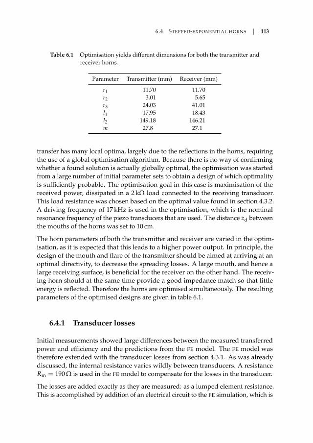
6.4 STEPPED-EXPONENTIAL HORNS 113
Table 6.1 Optimisation yields different dimensions for both the transmitter andreceiver horns.
Parameter Transmitter (mm) Receiver (mm)
r1 11.70 11.70r2 3.01 5.65r3 24.03 41.01l1 17.95 18.43l2 149.18 146.21m 27.8 27.1
transfer has many local optima, largely due to the reflections in the horns, requiringthe use of a global optimisation algorithm. Because there is no way of confirmingwhether a found solution is actually globally optimal, the optimisation was startedfrom a large number of initial parameter sets to obtain a design of which optimalityis sufficiently probable. The optimisation goal in this case is maximisation of thereceived power, dissipated in a 2 kΩ load connected to the receiving transducer.This load resistance was chosen based on the optimal value found in section 4.3.2.A driving frequency of 17 kHz is used in the optimisation, which is the nominalresonance frequency of the piezo transducers that are used. The distance zd betweenthe mouths of the horns was set to 10 cm.
The horn parameters of both the transmitter and receiver are varied in the optim-isation, as it is expected that this leads to a higher power output. In principle, thedesign of the mouth and flare of the transmitter should be aimed at arriving at anoptimal directivity, to decrease the spreading losses. A large mouth, and hence alarge receiving surface, is beneficial for the receiver on the other hand. The receiv-ing horn should at the same time provide a good impedance match so that littleenergy is reflected. Therefore the horns are optimised simultaneously. The resultingparameters of the optimised designs are given in table 6.1.
6.4.1 Transducer losses
Initial measurements showed large differences between the measured transferredpower and efficiency and the predictions from the FE model. The FE model wastherefore extended with the transducer losses from section 4.3.1. As was alreadydiscussed, the internal resistance varies wildly between transducers. A resistanceRm = 190 Ω is used in the FE model to compensate for the losses in the transducer.
The losses are added exactly as they are measured: as a lumped element resistance.This is accomplished by addition of an electrical circuit to the FE simulation, which is
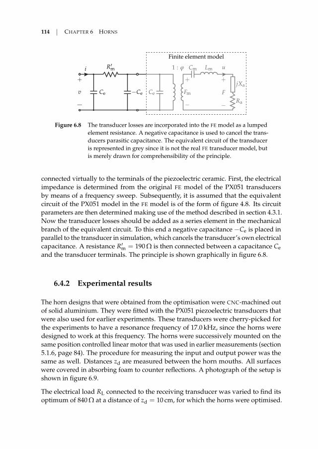
114 CHAPTER 6 HORNS
i
Finite element model
Ce
R′m
−Cev
+
−
LmCm u
Ra
jXa
1 : ϕ
Fm
+
−
F
+
−
Ce
Figure 6.8 The transducer losses are incorporated into the FE model as a lumpedelement resistance. A negative capacitance is used to cancel the trans-ducers parasitic capacitance. The equivalent circuit of the transduceris represented in grey since it is not the real FE transducer model, butis merely drawn for comprehensibility of the principle.
connected virtually to the terminals of the piezoelectric ceramic. First, the electricalimpedance is determined from the original FE model of the PX051 transducersby means of a frequency sweep. Subsequently, it is assumed that the equivalentcircuit of the PX051 model in the FE model is of the form of figure 4.8. Its circuitparameters are then determined making use of the method described in section 4.3.1.Now the transducer losses should be added as a series element in the mechanicalbranch of the equivalent circuit. To this end a negative capacitance −Ce is placed inparallel to the transducer in simulation, which cancels the transducer’s own electricalcapacitance. A resistance R′m = 190 Ω is then connected between a capacitance Ceand the transducer terminals. The principle is shown graphically in figure 6.8.
6.4.2 Experimental results
The horn designs that were obtained from the optimisation were CNC-machined outof solid aluminium. They were fitted with the PX051 piezoelectric transducers thatwere also used for earlier experiments. These transducers were cherry-picked forthe experiments to have a resonance frequency of 17.0 kHz, since the horns weredesigned to work at this frequency. The horns were successively mounted on thesame position controlled linear motor that was used in earlier measurements (section5.1.6, page 84). The procedure for measuring the input and output power was thesame as well. Distances zd are measured between the horn mouths. All surfaceswere covered in absorbing foam to counter reflections. A photograph of the setup isshown in figure 6.9.
The electrical load RL connected to the receiving transducer was varied to find itsoptimum of 840 Ω at a distance of zd = 10 cm, for which the horns were optimised.
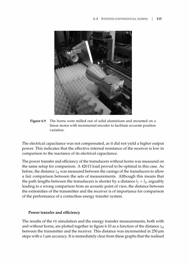
6.4 STEPPED-EXPONENTIAL HORNS 115
Figure 6.9 The horns were milled out of solid aluminium and mounted on alinear motor with incremental encoder to facilitate accurate positionvariation.
The electrical capacitance was not compensated, as it did not yield a higher outputpower. This indicates that the effective internal resistance of the receiver is low incomparison to the reactance of its electrical capacitance.
The power transfer and efficiency of the transducers without horns was measured onthe same setup for comparison. A 420 Ω load proved to be optimal in this case. Asbefore, the distance zd was measured between the casings of the transducers to allowa fair comparison between the sets of measurements. Although this means thatthe path lengths between the transducers is shorter by a distance l1 + l2, arguablyleading to a wrong comparison from an acoustic point of view, the distance betweenthe extremities of the transmitter and the receiver is of importance for comparisonof the performance of a contactless energy transfer system.
Power transfer and efficiency
The results of the FE simulation and the energy transfer measurements, both withand without horns, are plotted together in figure 6.10 as a function of the distance zdbetween the transmitter and the receiver. This distance was incremented in 250 µmsteps with a 1 µm accuracy. It is immediately clear from these graphs that the realised
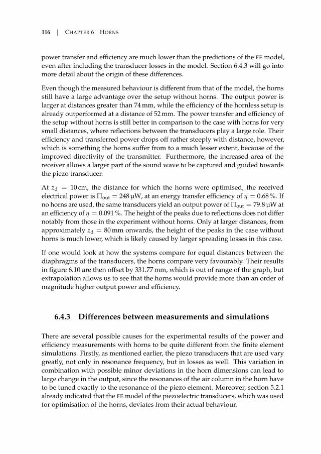
116 CHAPTER 6 HORNS
power transfer and efficiency are much lower than the predictions of the FE model,even after including the transducer losses in the model. Section 6.4.3 will go intomore detail about the origin of these differences.
Even though the measured behaviour is different from that of the model, the hornsstill have a large advantage over the setup without horns. The output power islarger at distances greater than 74 mm, while the efficiency of the hornless setup isalready outperformed at a distance of 52 mm. The power transfer and efficiency ofthe setup without horns is still better in comparison to the case with horns for verysmall distances, where reflections between the transducers play a large role. Theirefficiency and transferred power drops off rather steeply with distance, however,which is something the horns suffer from to a much lesser extent, because of theimproved directivity of the transmitter. Furthermore, the increased area of thereceiver allows a larger part of the sound wave to be captured and guided towardsthe piezo transducer.
At zd = 10 cm, the distance for which the horns were optimised, the receivedelectrical power is Πout = 248 µW, at an energy transfer efficiency of η = 0.68 %. Ifno horns are used, the same transducers yield an output power of Πout = 79.8 µW atan efficiency of η = 0.091 %. The height of the peaks due to reflections does not differnotably from those in the experiment without horns. Only at larger distances, fromapproximately zd = 80 mm onwards, the height of the peaks in the case withouthorns is much lower, which is likely caused by larger spreading losses in this case.
If one would look at how the systems compare for equal distances between thediaphragms of the transducers, the horns compare very favourably. Their resultsin figure 6.10 are then offset by 331.77 mm, which is out of range of the graph, butextrapolation allows us to see that the horns would provide more than an order ofmagnitude higher output power and efficiency.
6.4.3 Differences between measurements and simulations
There are several possible causes for the experimental results of the power andefficiency measurements with horns to be quite different from the finite elementsimulations. Firstly, as mentioned earlier, the piezo transducers that are used varygreatly, not only in resonance frequency, but in losses as well. This variation incombination with possible minor deviations in the horn dimensions can lead tolarge change in the output, since the resonances of the air column in the horn haveto be tuned exactly to the resonance of the piezo element. Moreover, section 5.2.1already indicated that the FE model of the piezoelectric transducers, which was usedfor optimisation of the horns, deviates from their actual behaviour.
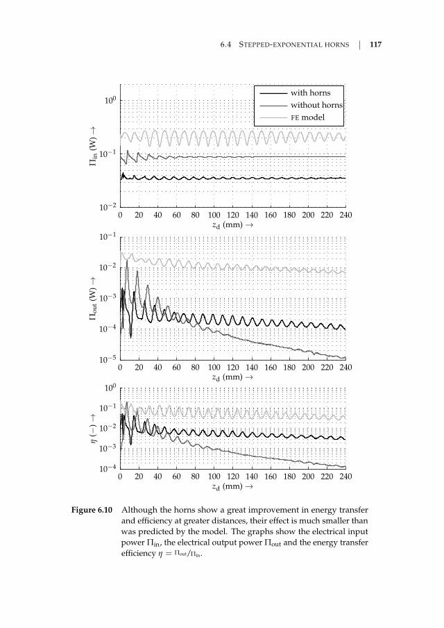
6.4 STEPPED-EXPONENTIAL HORNS 117
η
(−)→
zd (mm) →
Πo
ut
(W)→
zd (mm) →
FE model
without horns
with hornsΠ
in(W
)→
zd (mm) →
0 20 40 60 80 100 120 140 160 180 200 220 240
0 20 40 60 80 100 120 140 160 180 200 220 240
0 20 40 60 80 100 120 140 160 180 200 220 240
10−4
10−3
10−2
10−1
100
10−5
10−4
10−3
10−2
10−1
10−2
10−1
100
Figure 6.10 Although the horns show a great improvement in energy transferand efficiency at greater distances, their effect is much smaller thanwas predicted by the model. The graphs show the electrical inputpower Πin, the electrical output power Πout and the energy transferefficiency η = Πout/Πin.

118 CHAPTER 6 HORNS
Another possible effect that could degrade performance are viscous losses in thesmall cross-sectional areas of the exponential sections. The viscous and thermalboundary layer thicknesses at f = 17 kHz and 20 C are respectively [69]
dvis =
√2µ
ρ0ω= 16.9 µm (6.19a)
dth =
√2κ
ρ0ωcp= 19.9 µm , (6.19b)
with µ = 1.8369 · 10−5 kg m−1 s−1 being the viscosity, κ = 0.0257 W m−1 K−1 thethermal conductivity and cp = 1.005 · 103 J kg−1 K−1 the isobaric mass heat capacity,all of dry air at 20 C. These correspond to a viscous boundary layer covering1.1 % and a thermal boundary layer that makes up 1.3 % of the surface area at thenarrowest part (r = r2) of the transmitter horn. There will therefore be a smallinfluence due to viscous losses at the walls of the horns and heat exchange betweenthe horn and the air, but it is not expected to play a huge role.
Although nonlinear effects due to excessively high pressure levels are often respons-ible for reduced performance of horns, it was confirmed by measuring the linearitybetween the output sound pressure and the input voltage that this is not an issue inthe current design.
The influence of several other parameters will be investigated in the remainder ofthis section. The performance of the horns is judged based on the sensitivity S of thehorn driver (the piezo element-horn combination). It is defined in this case as the on-axis sound pressure amplitude2 at a distance of 10 cm from the horn mouth, dividedby the input voltage amplitude of the transducer. The sensitivity is measured bymeans of a Stanford Research Systems SR785 dynamic signal analyser using a sweptsine measurement. Only the ratio of the pressure and voltage amplitudes is retained,the phase information is discarded. The horns for the transmitting and the receivingtransducers are both used in a transmitting configuration for these tests.
Figure 6.11 beautifully illustrates the reason why losses were included in the finiteelement model, as the sensitivity without is much too high for both transducers.Adding a transducer loss resistance R′m = 190 Ω brings the simulated sensitivity ofthe receiver down to that of the measurements, but the sensitivity of the transmitter,as predicted by the FE model, is still too large.
Please keep in mind that the sensitivity is only used as a convenient quantity on thebasis of which to judge the deviation between the FE model and the measurements.
2The sound pressure was measured using a G.R.A.S. 40BF microphone, connected to a 26AC preampli-fier and a 12AK power module and postamplifier from the same manufacturer. The whole measurementchain is calibrated using a G.R.A.S. 42AA pistonphone.
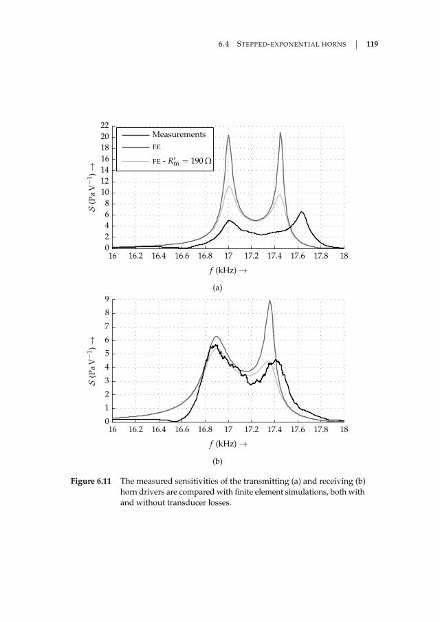
6.4 STEPPED-EXPONENTIAL HORNS 119
FE - R′m = 190 Ω
FE
Measurements
S(P
aV−
1)→
f (kHz) →
16 16.2 16.4 16.6 16.8 17 17.2 17.4 17.6 17.8 180
2
4
6
8
10
12
14
16
18
20
22
(a)
S(P
aV−
1)→
f (kHz) →
16 16.2 16.4 16.6 16.8 17 17.2 17.4 17.6 17.8 180
1
2
3
4
5
6
7
8
9
(b)
Figure 6.11 The measured sensitivities of the transmitting (a) and receiving (b)horn drivers are compared with finite element simulations, both withand without transducer losses.
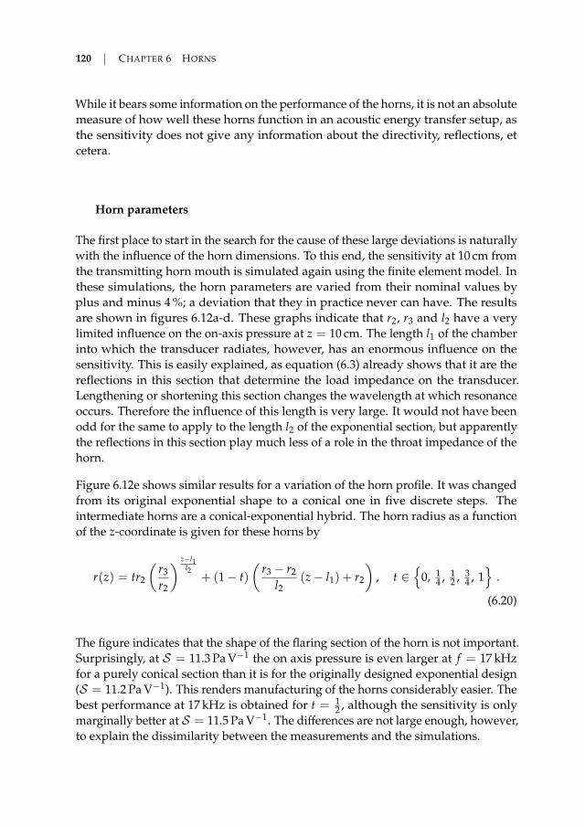
120 CHAPTER 6 HORNS
While it bears some information on the performance of the horns, it is not an absolutemeasure of how well these horns function in an acoustic energy transfer setup, asthe sensitivity does not give any information about the directivity, reflections, etcetera.
Horn parameters
The first place to start in the search for the cause of these large deviations is naturallywith the influence of the horn dimensions. To this end, the sensitivity at 10 cm fromthe transmitting horn mouth is simulated again using the finite element model. Inthese simulations, the horn parameters are varied from their nominal values byplus and minus 4 %; a deviation that they in practice never can have. The resultsare shown in figures 6.12a-d. These graphs indicate that r2, r3 and l2 have a verylimited influence on the on-axis pressure at z = 10 cm. The length l1 of the chamberinto which the transducer radiates, however, has an enormous influence on thesensitivity. This is easily explained, as equation (6.3) already shows that it are thereflections in this section that determine the load impedance on the transducer.Lengthening or shortening this section changes the wavelength at which resonanceoccurs. Therefore the influence of this length is very large. It would not have beenodd for the same to apply to the length l2 of the exponential section, but apparentlythe reflections in this section play much less of a role in the throat impedance of thehorn.
Figure 6.12e shows similar results for a variation of the horn profile. It was changedfrom its original exponential shape to a conical one in five discrete steps. Theintermediate horns are a conical-exponential hybrid. The horn radius as a functionof the z-coordinate is given for these horns by
r(z) = tr2
(r3
r2
) z−l1l2
+ (1− t)(
r3 − r2
l2(z− l1) + r2
), t ∈
0, 1
4 , 12 , 3
4 , 1
.
(6.20)
The figure indicates that the shape of the flaring section of the horn is not important.Surprisingly, at S = 11.3 Pa V−1 the on axis pressure is even larger at f = 17 kHzfor a purely conical section than it is for the originally designed exponential design(S = 11.2 Pa V−1). This renders manufacturing of the horns considerably easier. Thebest performance at 17 kHz is obtained for t = 1
2 , although the sensitivity is onlymarginally better at S = 11.5 Pa V−1. The differences are not large enough, however,to explain the dissimilarity between the measurements and the simulations.
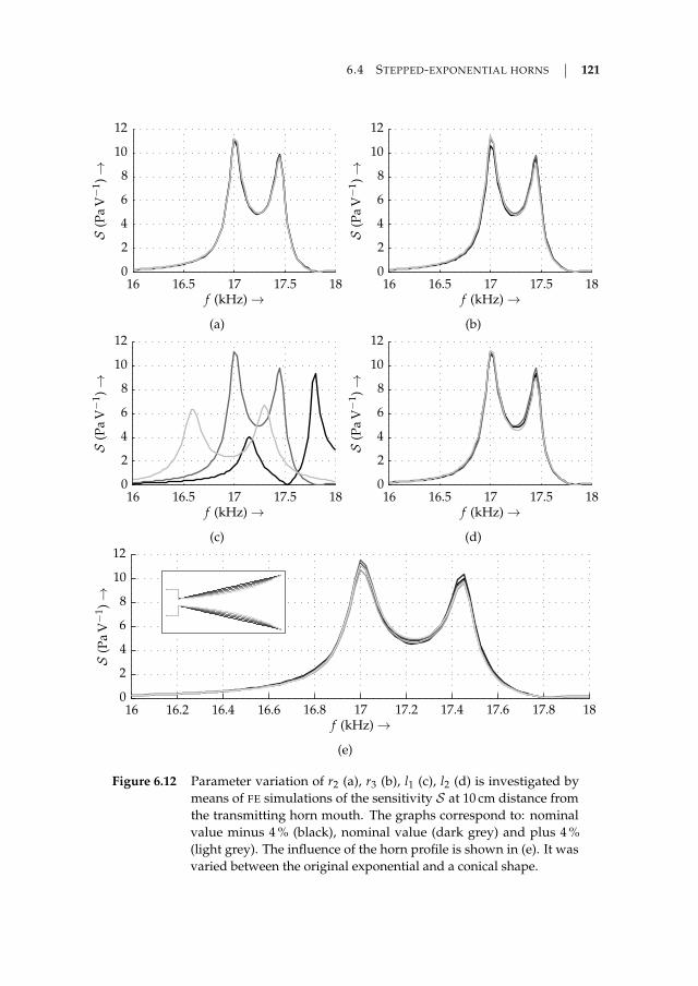
6.4 STEPPED-EXPONENTIAL HORNS 121
S(P
aV−
1)→
f (kHz) →16 16.5 17 17.5 18
0
2
4
6
8
10
12
(a)
S(P
aV−
1)→
f (kHz) →16 16.5 17 17.5 18
0
2
4
6
8
10
12
(b)
S(P
aV−
1)→
f (kHz) →16 16.5 17 17.5 18
0
2
4
6
8
10
12
(c)
S(P
aV−
1)→
f (kHz) →16 16.5 17 17.5 18
0
2
4
6
8
10
12
(d)
S(P
aV−
1)→
f (kHz) →16 16.2 16.4 16.6 16.8 17 17.2 17.4 17.6 17.8 18
0
2
4
6
8
10
12
(e)
Figure 6.12 Parameter variation of r2 (a), r3 (b), l1 (c), l2 (d) is investigated bymeans of FE simulations of the sensitivity S at 10 cm distance fromthe transmitting horn mouth. The graphs correspond to: nominalvalue minus 4 % (black), nominal value (dark grey) and plus 4 %(light grey). The influence of the horn profile is shown in (e). It wasvaried between the original exponential and a conical shape.
122 CHAPTER 6 HORNS
Transducer losses
Figure 6.11 already gave a quick first glance at how transducer losses influence thecharacteristics of the stepped-exponential horn radiators. Understandably, the losseslower the sensitivity, owing to the fact that part of the energy is dissipated in thetransducer, rather than radiated.
Figure 6.13 gives a better view of the influence of the transducer losses. The sens-itivity indeed decreases when the losses increase. Since the mechanical qualityfactor Qm of the transducer also decreases (see equation (4.34)), the sharpness of theresonance peaks decreases when the resistance is increased.
As said before, the sensitivity of the receiving horn and transducer match very wellwith the simulation results for R′m = 190 Ω, but those of the transmitting horn donot. They are still more than a factor two off. It is not possible to get both to matchonly by addition of transducer losses. These losses will therefore play a role in thediscrepancy between measurements and model, but will not be the sole cause.
Interestingly enough, especially from figure 6.13b, it appears that the right peak,around 17.4 kHz, is damped much more by the transducer losses than the left one.This effect is much less pronounced for the transmitter (figure 6.13a).
Piezoelectric stress constant
Section 5.2 mentioned that, based on the relative permittivity of the piezoelectricmaterial, it is probable that an incorrect material is used in the finite element model.Let us therefore have a look at how the piezoelectric stress constant influences thesensitivity of the horn drivers, and whether a wrongly chosen value in the FE modelcan cause the deviations seen in figure 6.11.
The finite element model uses PZT-5A as a piezoelectric material, as was indicatedin the previous chapter. The PZT-5A material that is available in the material libraryin Comsol Mulitphysics has e31 = −5.35 C m−2 and e33 = 15.78 C m−2. Both valuesare changed in simulation to investigate their impact on the sensitivity. The 31-component is changed to −2 C m−2 and e33 to 5 C m−2; first separately, then bothcomponents are changed simultaneously. The effect of e15 was already shownto be minimal, as one would expect from a bender element, and is therefore notconsidered.
Figure 6.14 depicts the sensitivity at a 10 cm distance from the horn mouth for thesecombinations of stress constants. Decreasing the stress constant leads to a lowersensitivity, as is to be expected, since it is the factor relating the stress to the electricfield. Altering the stress constant also changes the resonance frequencies of the
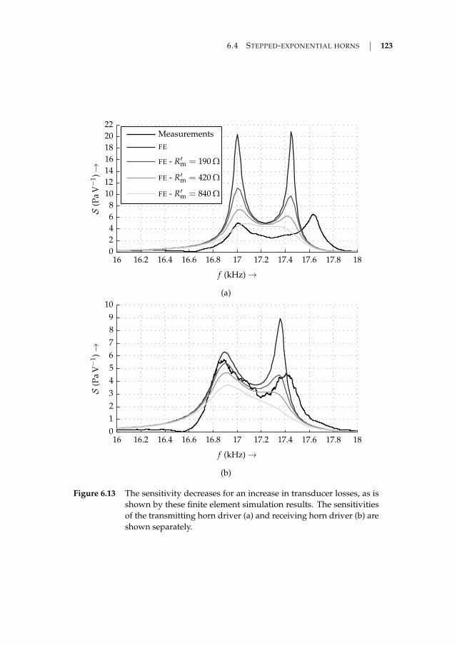
6.4 STEPPED-EXPONENTIAL HORNS 123
FE - R′m = 840 Ω
FE - R′m = 420 Ω
FE - R′m = 190 Ω
FE
Measurements
S(P
aV−
1)→
f (kHz) →
16 16.2 16.4 16.6 16.8 17 17.2 17.4 17.6 17.8 180
2
4
6
8
10
12
14
16
18
20
22
(a)
S(P
aV−
1)→
f (kHz) →
16 16.2 16.4 16.6 16.8 17 17.2 17.4 17.6 17.8 180
1
2
3
4
5
6
7
8
9
10
(b)
Figure 6.13 The sensitivity decreases for an increase in transducer losses, as isshown by these finite element simulation results. The sensitivitiesof the transmitting horn driver (a) and receiving horn driver (b) areshown separately.
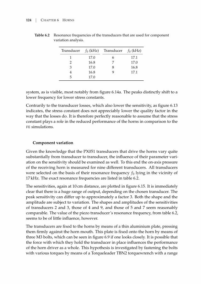
124 CHAPTER 6 HORNS
Table 6.2 Resonance frequencies of the transducers that are used for componentvariation analysis.
Transducer f0 (kHz) Transducer f0 (kHz)
1 17.0 6 17.12 16.8 7 17.03 17.0 8 16.84 16.8 9 17.15 17.0
system, as is visible, most notably from figure 6.14a. The peaks distinctly shift to alower frequency for lower stress constants.
Contrarily to the transducer losses, which also lower the sensitivity, as figure 6.13indicates, the stress constant does not appreciably lower the quality factor in theway that the losses do. It is therefore perfectly reasonable to assume that the stressconstant plays a role in the reduced performance of the horns in comparison to theFE simulations.
Component variation
Given the knowledge that the PX051 transducers that drive the horns vary quitesubstantially from transducer to transducer, the influence of their parameter vari-ation on the sensitivity should be examined as well. To this end the on-axis pressureof the receiving horn is measured for nine different transducers. All transducerswere selected on the basis of their resonance frequency f0 lying in the vicinity of17 kHz. The exact resonance frequencies are listed in table 6.2.
The sensitivities, again at 10 cm distance, are plotted in figure 6.15. It is immediatelyclear that there is a huge range of output, depending on the chosen transducer. Thepeak sensitivity can differ up to approximately a factor 3. Both the shape and theamplitude are subject to variation. The shapes and amplitudes of the sensitivitiesof transducers 2 and 3, those of 4 and 9, and those of 5 and 7 seem reasonablycomparable. The value of the piezo transducer’s resonance frequency, from table 6.2,seems to be of little influence, however.
The transducers are fixed to the horns by means of a thin aluminium plate, pressingthem firmly against the horn mouth. This plate is fixed onto the horn by means ofthree M3 bolts, which can be seen in figure 6.9 if one looks closely. It is possible thatthe force with which they hold the transducer in place influences the performanceof the horn driver as a whole. This hypothesis is investigated by fastening the boltswith various torques by means of a Torqueleader TBN2 torquewrench with a range
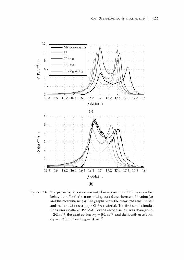
6.4 STEPPED-EXPONENTIAL HORNS 125
FE - e31 & e33
FE - e33
FE - e31
FE
Measurements
S(P
aV−
1)→
f (kHz) →
15.8 16 16.2 16.4 16.6 16.8 17 17.2 17.4 17.6 17.8 180
2
4
6
8
10
12
(a)
S(P
aV−
1)→
f (kHz) →
15.8 16 16.2 16.4 16.6 16.8 17 17.2 17.4 17.6 17.8 180
1
2
3
4
5
6
(b)
Figure 6.14 The piezoelectric stress constant e has a pronounced influence on thebehaviour of both the transmitting transducer-horn combination (a)and the receiving set (b). The graphs show the measured sensitivitiesand FE simulations using PZT-5A material. The first set of simula-tions uses unaltered PZT-5A. For the second set e31 was changed to−2 C m−2, the third set has e33 = 5 C m−2, and the fourth uses bothe31 = −2 C m−2 and e33 = 5 C m−2.
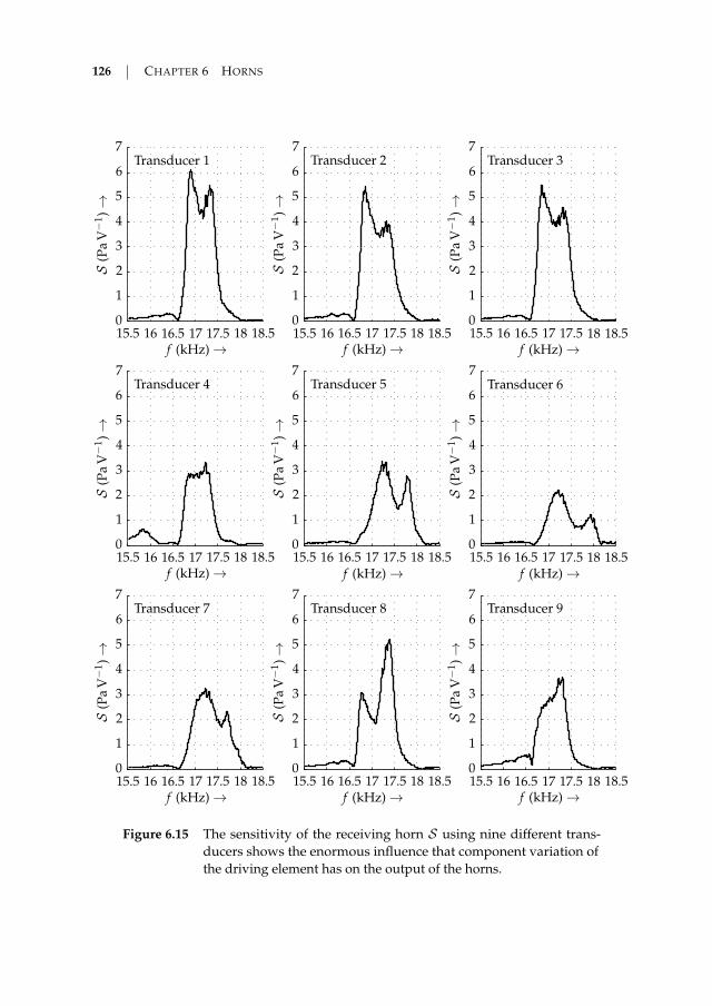
126 CHAPTER 6 HORNS
S(P
aV−
1)→
f (kHz) →
S(P
aV−
1)→
f (kHz) →
S(P
aV−
1)→
f (kHz) →
S(P
aV−
1)→
f (kHz) →
S(P
aV−
1)→
f (kHz) →
S(P
aV−
1)→
f (kHz) →
S(P
aV−
1)→
f (kHz) →
S(P
aV−
1)→
f (kHz) →
S(P
aV−
1)→
f (kHz) →
Transducer 9Transducer 8Transducer 7
Transducer 6Transducer 5Transducer 4
Transducer 3Transducer 2Transducer 1
15.5 16 16.5 17 17.5 18 18.515.5 16 16.5 17 17.5 18 18.515.5 16 16.5 17 17.5 18 18.5
15.5 16 16.5 17 17.5 18 18.515.5 16 16.5 17 17.5 18 18.515.5 16 16.5 17 17.5 18 18.5
15.5 16 16.5 17 17.5 18 18.515.5 16 16.5 17 17.5 18 18.515.5 16 16.5 17 17.5 18 18.5
0
1
2
3
4
5
6
7
0
1
2
3
4
5
6
7
0
1
2
3
4
5
6
7
0
1
2
3
4
5
6
7
0
1
2
3
4
5
6
7
0
1
2
3
4
5
6
7
0
1
2
3
4
5
6
7
0
1
2
3
4
5
6
7
0
1
2
3
4
5
6
7
Figure 6.15 The sensitivity of the receiving horn S using nine different trans-ducers shows the enormous influence that component variation ofthe driving element has on the output of the horns.
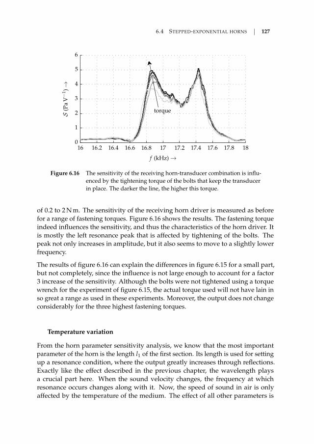
6.4 STEPPED-EXPONENTIAL HORNS 127
S(P
aV−
1)→
f (kHz) →
torque
16 16.2 16.4 16.6 16.8 17 17.2 17.4 17.6 17.8 180
1
2
3
4
5
6
Figure 6.16 The sensitivity of the receiving horn-transducer combination is influ-enced by the tightening torque of the bolts that keep the transducerin place. The darker the line, the higher this torque.
of 0.2 to 2 N m. The sensitivity of the receiving horn driver is measured as beforefor a range of fastening torques. Figure 6.16 shows the results. The fastening torqueindeed influences the sensitivity, and thus the characteristics of the horn driver. Itis mostly the left resonance peak that is affected by tightening of the bolts. Thepeak not only increases in amplitude, but it also seems to move to a slightly lowerfrequency.
The results of figure 6.16 can explain the differences in figure 6.15 for a small part,but not completely, since the influence is not large enough to account for a factor3 increase of the sensitivity. Although the bolts were not tightened using a torquewrench for the experiment of figure 6.15, the actual torque used will not have lain inso great a range as used in these experiments. Moreover, the output does not changeconsiderably for the three highest fastening torques.
Temperature variation
From the horn parameter sensitivity analysis, we know that the most importantparameter of the horn is the length l1 of the first section. Its length is used for settingup a resonance condition, where the output greatly increases through reflections.Exactly like the effect described in the previous chapter, the wavelength playsa crucial part here. When the sound velocity changes, the frequency at whichresonance occurs changes along with it. Now, the speed of sound in air is onlyaffected by the temperature of the medium. The effect of all other parameters is
128 CHAPTER 6 HORNS
negligible [58]. Since the measurements in this chapter were done in a period werethe maximum ambient temperature lay at 25 C or higher, let us choose this value asa reference value to investigate the influence of the temperature.
The equation of state for a perfect gas is, according to [58], equal to
pt = ρtrTK (6.21)
with r ≈ 287.06 J kg−1 K−1 the specific gas constant and TK the absolute temperaturein Kelvins. Combination with (3.7b) allows the sound velocity to be written as
c2 = γrTK
= c20
(1 +
TT0
) (6.22)
where c0 is the sound velocity at 0 C, T is the temperature in C and T0 = 273.15 K.From equation (3.7b), and the list of physical constants in A.5, we can calculate thesound velocity at 0 C to be c0 = 331.33 m s−1.
To obtain a resonance condition, the length l1 of the first section of the horn must beapproximately half a wavelength. Therefore we have
l1 ≈ 12
c20 Cf20 C
= 12
c25 Cf25 C
, (6.23)
or
f25 Cf20 C
=
√T0 + 25 CT0 + 20 C
≈ 1.00849 .
(6.24)
The horns were designed for a frequency f20 C = 17 kHz, which implies that theshift in resonance frequency is f25 C − f20 C ≈ 144.3 Hz. Suppose we would choosethis to be equal to the 3 dB bandwidth, or, in other words, that only half the poweris available at 17 kHz and 25 C. In that case the corresponding quality factor is
Q = 12
17 kHz144.3 Hz
≈ 59 . (6.25)
This is a very low quality factor for a piezoelectric transducer. It is therefore veryprobable that the temperature is a main contributor to the differences between themeasurements and the modelled behaviour.

6.5 CONCLUSIONS AND DISCUSSION 129
6.5 Conclusions and discussion
This chapter investigated the use of horns in an acoustic energy transfer system inan attempt to improve the energy throughput in such a system and to reduce thereflections that were shown to be of a large influence. First measurements using asimple nonoptimised horn design indicated that the addition of horns to an existingAET system has enough interesting effects to warrant a further investigation of theirinfluence. Although they did not reduce reflections, they significantly improved theefficiency at greater distances because of the increased directivity of the transmitterand the enlarged surface of the receiver.
Stepped exponential horns were successively designed for the transmitter and thereceiver of an acoustic energy transfer system to boost the output power and theenergy transfer efficiency. The profile of these horns follows a stepwise change inradius, which is used to boost the throat impedance, followed by a section thatflares out exponentially, whose purpose is the optimisation of the directivity of thetransmitter and the surface of the receiver. Optimisation of the electrical outputpower was performed using a global optimisation algorithm in combination with afinite element model of the horns and the piezoelectric transducers.
Initial measurements of the energy transfer showed a significant deviation in powerlevels from those predicted by the finite element model. Losses in the transducerswere therefore added to the model in the form of an equivalent resistance. Thisresistance alone proved not sufficient to explain the difference, as the measuredpower transfer and energy transfer efficiency were still much lower than simulationsindicated. Still, the effect of the horns is evident, especially at greater distancesbetween the transmitter and the receiver. At zd = 10.0 cm—the distance betweenthe transmitter and receiver for which the horns were designed—the addition of thehorns results in an output power that is approximately 3.1 times higher while theefficiency is 7.5 times higher in comparison to measurements without horns.
Various possible sources of the discrepancy between the measured energy transferand that predicted by simulations were investigated. Losses, as mentioned earlier,are a part of the cause, but it is shown in this chapter that they cannot solely make upfor the difference. Bringing the simulated sensitivities of the transducers with hornsdown to the level of the measurement requires adding so high a loss resistance thatresonance peaks completely disappear because of a much reduced quality factor.
It was shown that the piezoelectric stress constant can account for a large variationin output of the order of the observed difference. Unlike the transducer losses,this constant can bring the sensitivities down to the measured amplitudes, withoutcompromising the resonance peaks. Taking into consideration that the piezoelectricmaterial used in the transducers is unknown, and, moreover, already shown to be
130 CHAPTER 6 HORNS
different from the material used in simulation (see page 90), there is a fair chance thata large part of the discrepancies is to be attributed to an incorrect transducer model.Again, this goes to show that transducer identification is critical for AET systemmodelling, and must occur before designing impedance adaptation measures.
Not only are the materials of the piezoelectric transducers unknown, even the com-ponent variation between transducers proves to be a large problem. Swappingtransducers makes a large difference, not only in output, but in frequency responseas well. There is no discernable connection between the transducer’s resonancefrequency and the obtained sensitivity plot. It was even found that the same trans-ducer could give a slightly different output when remounting. All in all, the poorreproducibility was ultimately the reason why the experiments were stopped.
Of all horn parameters, only the length l1 of the first section of the horn has a distinctinfluence on the output. Reflections in this section greatly boost the impedanceseen by the transducer. In hindsight this was not necessarily a good choice, as thesystem’s sensitivity to parameter variation is enormous. Especially the combinationwith temperature variation will influence the output to a large extent. It was shownthat a temperature rise of 5 C implies half the output power is obtained if the hornis coupled to a component with a quality factor of 59. It is therefore expected that thevariation of this resonance frequency is one of the main contributors to the observeddifferences, although, unfortunately, this has not been verified.
It would have been better to investigate the impact of horns on the AET energytransfer using a length l1 that is very short in comparison to the wavelength, as isconventionally done in horn loudspeaker systems [15]. The disadvantage in thiscase is that there is no resonance that can be used to boost the impedance, while theadvantage is that there is no resonance that can cause mismatch problems. The step-wise change in radius can still be utilised for impedance transformation according toequation (6.2) in this case. If one does choose to work with multiple components thatshould resonate at the same frequency, adjustability of these resonance frequenciesis a must.
Another principle that is used in horns for audio purposes is the addition of a phas-ing plug [15, 20], that equalises path lengths from different parts of the transducerdiaphragm to the throat of the horn. At certain frequencies these path length differ-ences, when unequal, can cause interference when the size of the diaphragm is of theorder of a wavelength or larger. Sound waves from the edge of the diaphragm canthen (partly) cancel those emitted from the centre. Possibly this leads to a decreasedoutput when the resonance frequency changes. The finite element model did notpredict the telltale notches in the frequency response that give away this problem.The principle was therefore not researched further.
A third principle used in horns for loudspeakers is the addition of a compression

6.5 CONCLUSIONS AND DISCUSSION 131
chamber behind the diaphragm. Without it, the diaphragm experiences a largeopposing pressure from the impedance transformation by the horn when it moves inthe forward direction. When it moves backwards, however, it only has to counteractthe free air radiation impedance. This can lead to nonlinearity, which in audioapplications is of course extremely undesirable. Nonlinearity was found to be not anissue in the experiments so far. If the horns are to be used at larger output levels itmay become necessary to add a compression chamber at the back of the transducer,which adds a stiffness component that counteracts this nonlinearity.
Lastly, it was shown that the profile of the section that flares out from a small radiusr2 to a larger horn mouth radius r3 is not critical at all. A conical horn can be usedinstead of the chosen exponential shape without problems, and will even result in ahigher sensitivity. Such a horn is much easier to manufacture when turning it formmetal, just as the the horns in this chapter. It is not a particularly large problemthough, as modern 3D printing technology can produce about any desired shape.Keep in mind that the sensitivity does not give any information about the directivityof the horn and the effect it has on reflections. Here an exponential section may stillprove to be advantageous.

CH
AP
TE
R
7 Experiments withbolt-clamped Langevintransducers
LOUDSPEAKERS make use of the high radiation resistance that the large surfaceof their diaphragms offers. The sound that would be produced by the voice coil
alone would be barely noticeable, but the loudspeaker’s cone can produce animpressive sound volume. The diaphragm couples the vibrations of the small voicecoil to a considerable volume of air, making it a very effective method of impedancematching. This principle of impedance adaptation by means of a change in surfacearea can also be employed in acoustic energy transfer to match the transmittingand receiving transducers to the medium. It is used in this chapter in an attempt toincrease the output power.
Let us suppose that we have a radiator that moves against a counteracting pressure.The force that it has to exert is equal to the product of this pressure and its surfacearea, F = pA. The pressure is, however, not constant, but is linked with thetransducer’s directivity, which increases with the radiating surface area. Thereforethe radiation resistance grows faster than linearly with the surface area of the radiator.This can be seen in figure 4.3.
The experiments that have been discussed up to this point all leave something tobe desired, mostly in terms of output power and efficiency, but also in terms ofreproducibility. Different transducers are used in this chapter in an attempt to boostthe output power and to increase the reproducibility. Bolt-clamped Langevin trans-ducers (BLT) [125] were chosen for this purpose. These are 33-mode piezoelectricactuators, which are comprised of one or more piezoelectric rings, attached to ametal front and back mass that are used for tuning of the transducer’s resonancefrequency (see figure 7.1). This topology addresses a major issue of piezoelectric
133

134 CHAPTER 7 EXPERIMENTS WITH BOLT-CLAMPED LANGEVIN TRANSDUCERS
front mass
back mass
piezo rings
Figure 7.1 The Steiner & Martins SMBLTD45F40H transducers that are used inthis chapter consist of two piezoelectric discs between an aluminiumfront and back mass, held together by a bolt that applies a prestress.
transducers, namely the low power handling capabilities of piezoelectric material.While these materials can stand compressive stress very well, they crack very easilyunder tensile stress. A bolt that connects the front and back masses is used to ap-ply a prestress in the BLT topology, making it suitable for high power applications.Moreover, the transducer topology is typically very efficient if hard PZT material isused.
All experiments in this chapter make use of Steiner & Martins SMBLTD45F40Hbolt-clamped Langevin transducers, a photograph of which can be seen in figure7.1. Aluminium plates are bolted to the transducers to increase their radiating andreceiving surface areas. Plates of various radii and thicknesses are used so that theinfluence of the plate dimensions can be investigated. The radius of a plate r is either40 mm, 70 mm or 100 mm, while the thickness d can be 1 mm, 5 mm or 10 mm. Ashorthand notation r/d is used in this chapter to indicate specific plates, e.g. a 70/10plate would be of 70 mm radius and have a thickness of 10 mm. In the experiments,the transmitter and receiver were always fitted with the same plates.
This chapter discusses energy transfer measurements of the transducers with andwithout plates, as well as peculiarities that were encountered during the measure-ments.
7.1 Reflections
All previous measurements were done at a fixed driving frequency, while the dis-tance between the transmitter and the receiver was varied. This is a logical approach,
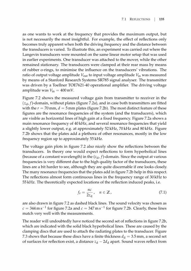
7.1 REFLECTIONS 135
as one wants to work at the frequency that provides the maximum output, butis not necessarily the most insightful. For example, the effect of reflections onlybecomes truly apparent when both the driving frequency and the distance betweenthe transducers is varied. To illustrate this, an experiment was carried out where theLangevin transducers were mounted on the same linear motor setup that was usedin earlier experiments. One transducer was attached to the mover, while the otherremained stationary. The transducers were clamped at their rear mass by meansof rubber o-rings, to minimise the influence on the transducers’ vibrations. Theratio of output voltage amplitude Vout to input voltage amplitude Vin was measuredby means of a Stanford Research Systems SR785 signal analyser. The transmitterwas driven by a Toellner TOE7621-40 operational amplifier. The driving voltageamplitude was Vin = 400 mV.
Figure 7.2 shows the measured voltage gain from transmitter to receiver in the(zd, f )-domain, without plates (figure 7.2a), and in case both transmitters are fittedwith the r = 70 mm, d = 5 mm plates (figure 7.2b). The most distinct feature of thesefigures are the resonance frequencies of the system (and the transducers), whichare visible as horizontal lines of high gain at a fixed frequency. Figure 7.2a shows amain resonance frequency of 40 kHz, and several resonance frequencies that yielda slightly lower output, e.g. at approximately 52 kHz, 70 kHz and 80 kHz. Figure7.2b shows that the plates add a plethora of other resonances, mostly in the lowfrequency region up to approximately 55 kHz.
The voltage gain plots in figure 7.2 also nicely show the reflections between thetransducers. In theory one would expect reflections to form hyperbolical lines(because of a constant wavelength) in the (zd, f )-domain. Since the output at variousfrequencies is very different due to the high quality factor of the transducers, theselines are a bit harder to see, although they are quite discernable if one looks closely.The many resonance frequencies that the plates add in figure 7.2b help in this respect.The reflections almost form continuous lines in the frequency range of 30 kHz to55 kHz. The theoretically expected locations of the reflection induced peaks, i.e.
fr =nc2zd
, n ∈ Z , (7.1)
are also drawn in figure 7.2 as dashed black lines. The sound velocity was chosen asc = 344 m s−1 for figure 7.2a and c = 347 m s−1 for figure 7.2b. Clearly, these linesmatch very well with the measurements.
The reader will undoubtedly have noticed the second set of reflections in figure 7.2b,which are indicated with the solid black hyperbolical lines. These are caused by theclamping discs that are used to attach the radiating plates to the transducer. Figure7.3 shows that because these discs have a finite thickness dd = 3.5 mm, a second setof surfaces for reflection exist, a distance zd − 2dd apart. Sound waves reflect from

136 CHAPTER 7 EXPERIMENTS WITH BOLT-CLAMPED LANGEVIN TRANSDUCERS
20lo
g10|V
ou
t /V
in|
(dB
)→
f(k
Hz)
→
zd (mm) →20 25 30 35 40 45
−170
−160
−150
−140
−130
−120
−110
−100
−90
−80
−70
−60
−50
−40
30
40
50
60
70
80
90
100
(a)
20lo
g10|V
ou
t /V
in|
(dB
)→
f(k
Hz)
→
zd (mm) →10 15 20 25 30 35
−130
−120
−110
−100
−90
−80
−70
−60
−50
−40
30
40
50
60
70
80
90
100
(b)
Figure 7.2 The voltage transfer ratio of receiver output voltage to transmitterinput voltage as a function of the distance zd between the two and thedriving frequency for a system without plates (a) and with 70/5 plates(b). The expected location of the reflections in the (zd, f )-domainis indicated by the dashed black lines. The solid black lines in (b)correspond to reflections between the discs that affix the plates to thetransducers.
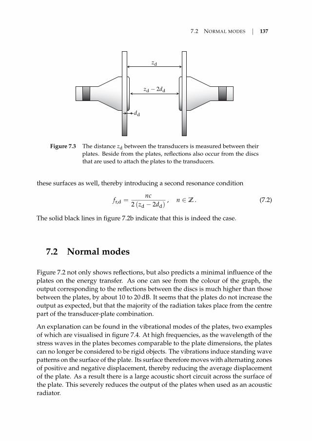
7.2 NORMAL MODES 137
zd
zd − 2dd
dd
Figure 7.3 The distance zd between the transducers is measured between theirplates. Beside from the plates, reflections also occur from the discsthat are used to attach the plates to the transducers.
these surfaces as well, thereby introducing a second resonance condition
fr,d =nc
2 (zd − 2dd), n ∈ Z . (7.2)
The solid black lines in figure 7.2b indicate that this is indeed the case.
7.2 Normal modes
Figure 7.2 not only shows reflections, but also predicts a minimal influence of theplates on the energy transfer. As one can see from the colour of the graph, theoutput corresponding to the reflections between the discs is much higher than thosebetween the plates, by about 10 to 20 dB. It seems that the plates do not increase theoutput as expected, but that the majority of the radiation takes place from the centrepart of the transducer-plate combination.
An explanation can be found in the vibrational modes of the plates, two examplesof which are visualised in figure 7.4. At high frequencies, as the wavelength of thestress waves in the plates becomes comparable to the plate dimensions, the platescan no longer be considered to be rigid objects. The vibrations induce standing wavepatterns on the surface of the plate. Its surface therefore moves with alternating zonesof positive and negative displacement, thereby reducing the average displacementof the plate. As a result there is a large acoustic short circuit across the surface ofthe plate. This severely reduces the output of the plates when used as an acousticradiator.
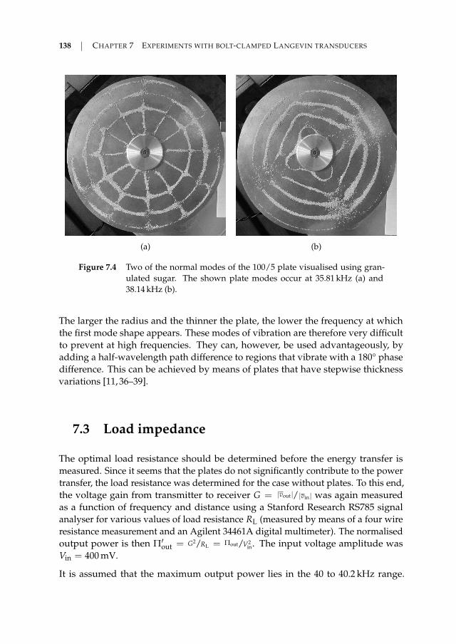
138 CHAPTER 7 EXPERIMENTS WITH BOLT-CLAMPED LANGEVIN TRANSDUCERS
(a) (b)
Figure 7.4 Two of the normal modes of the 100/5 plate visualised using gran-ulated sugar. The shown plate modes occur at 35.81 kHz (a) and38.14 kHz (b).
The larger the radius and the thinner the plate, the lower the frequency at whichthe first mode shape appears. These modes of vibration are therefore very difficultto prevent at high frequencies. They can, however, be used advantageously, byadding a half-wavelength path difference to regions that vibrate with a 180° phasedifference. This can be achieved by means of plates that have stepwise thicknessvariations [11, 36–39].
7.3 Load impedance
The optimal load resistance should be determined before the energy transfer ismeasured. Since it seems that the plates do not significantly contribute to the powertransfer, the load resistance was determined for the case without plates. To this end,the voltage gain from transmitter to receiver G = |vout|/|vin| was again measuredas a function of frequency and distance using a Stanford Research RS785 signalanalyser for various values of load resistance RL (measured by means of a four wireresistance measurement and an Agilent 34461A digital multimeter). The normalisedoutput power is then Π′out = G2/RL = Πout/V2
in. The input voltage amplitude wasVin = 400 mV.
It is assumed that the maximum output power lies in the 40 to 40.2 kHz range.
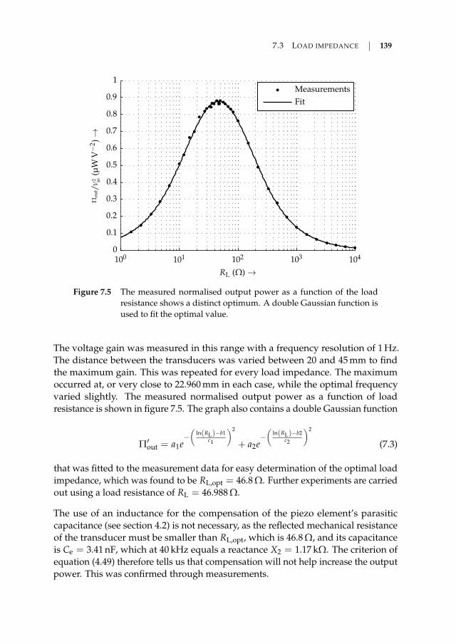
7.3 LOAD IMPEDANCE 139
Fit
MeasurementsΠ
ou
t /V
2 in(µ
WV−
2)→
RL (Ω) →
100 101 102 103 1040
0.1
0.2
0.3
0.4
0.5
0.6
0.7
0.8
0.9
1
Figure 7.5 The measured normalised output power as a function of the loadresistance shows a distinct optimum. A double Gaussian function isused to fit the optimal value.
The voltage gain was measured in this range with a frequency resolution of 1 Hz.The distance between the transducers was varied between 20 and 45 mm to findthe maximum gain. This was repeated for every load impedance. The maximumoccurred at, or very close to 22.960 mm in each case, while the optimal frequencyvaried slightly. The measured normalised output power as a function of loadresistance is shown in figure 7.5. The graph also contains a double Gaussian function
Π′out = a1e−(
ln(RL)−b1c1
)2
+ a2e−(
ln(RL)−b2c2
)2
(7.3)
that was fitted to the measurement data for easy determination of the optimal loadimpedance, which was found to be RL,opt = 46.8 Ω. Further experiments are carriedout using a load resistance of RL = 46.988 Ω.
The use of an inductance for the compensation of the piezo element’s parasiticcapacitance (see section 4.2) is not necessary, as the reflected mechanical resistanceof the transducer must be smaller than RL,opt, which is 46.8 Ω, and its capacitanceis Ce = 3.41 nF, which at 40 kHz equals a reactance X2 = 1.17 kΩ. The criterion ofequation (4.49) therefore tells us that compensation will not help increase the outputpower. This was confirmed through measurements.
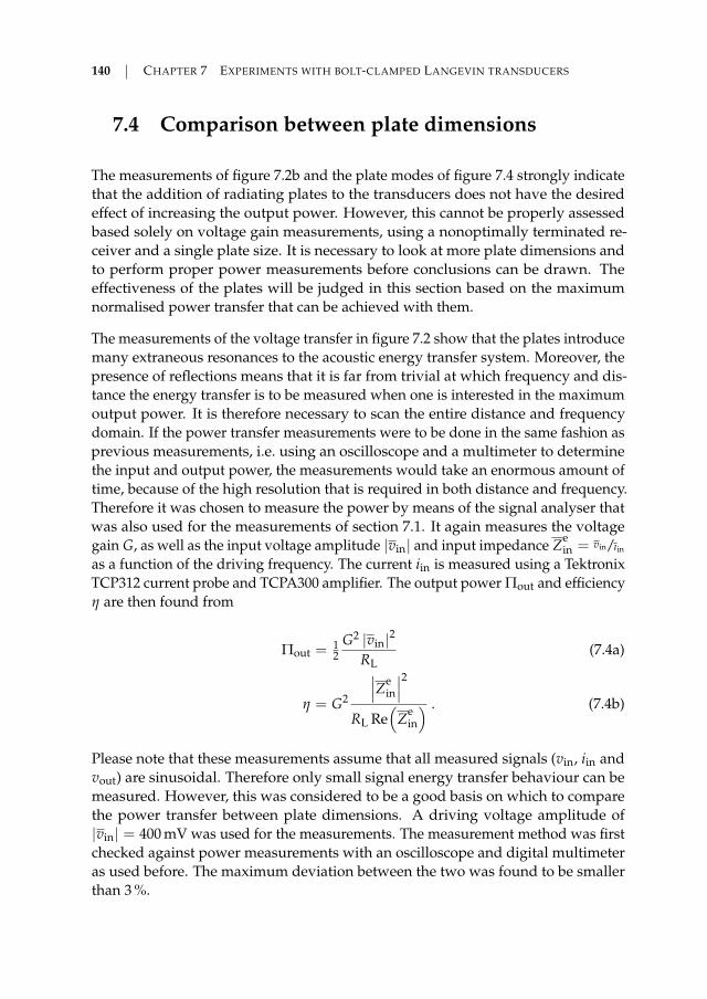
140 CHAPTER 7 EXPERIMENTS WITH BOLT-CLAMPED LANGEVIN TRANSDUCERS
7.4 Comparison between plate dimensions
The measurements of figure 7.2b and the plate modes of figure 7.4 strongly indicatethat the addition of radiating plates to the transducers does not have the desiredeffect of increasing the output power. However, this cannot be properly assessedbased solely on voltage gain measurements, using a nonoptimally terminated re-ceiver and a single plate size. It is necessary to look at more plate dimensions andto perform proper power measurements before conclusions can be drawn. Theeffectiveness of the plates will be judged in this section based on the maximumnormalised power transfer that can be achieved with them.
The measurements of the voltage transfer in figure 7.2 show that the plates introducemany extraneous resonances to the acoustic energy transfer system. Moreover, thepresence of reflections means that it is far from trivial at which frequency and dis-tance the energy transfer is to be measured when one is interested in the maximumoutput power. It is therefore necessary to scan the entire distance and frequencydomain. If the power transfer measurements were to be done in the same fashion asprevious measurements, i.e. using an oscilloscope and a multimeter to determinethe input and output power, the measurements would take an enormous amount oftime, because of the high resolution that is required in both distance and frequency.Therefore it was chosen to measure the power by means of the signal analyser thatwas also used for the measurements of section 7.1. It again measures the voltagegain G, as well as the input voltage amplitude |vin| and input impedance Ze
in = vin/ıin
as a function of the driving frequency. The current iin is measured using a TektronixTCP312 current probe and TCPA300 amplifier. The output power Πout and efficiencyη are then found from
Πout =12
G2 |vin|2
RL(7.4a)
η = G2
∣∣∣Zein
∣∣∣2RL Re
(Ze
in
) . (7.4b)
Please note that these measurements assume that all measured signals (vin, iin andvout) are sinusoidal. Therefore only small signal energy transfer behaviour can bemeasured. However, this was considered to be a good basis on which to comparethe power transfer between plate dimensions. A driving voltage amplitude of|vin| = 400 mV was used for the measurements. The measurement method was firstchecked against power measurements with an oscilloscope and digital multimeteras used before. The maximum deviation between the two was found to be smallerthan 3 %.
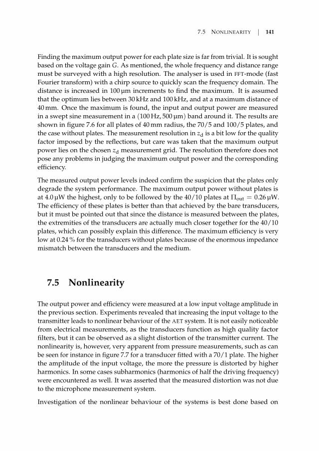
7.5 NONLINEARITY 141
Finding the maximum output power for each plate size is far from trivial. It is soughtbased on the voltage gain G. As mentioned, the whole frequency and distance rangemust be surveyed with a high resolution. The analyser is used in FFT-mode (fastFourier transform) with a chirp source to quickly scan the frequency domain. Thedistance is increased in 100 µm increments to find the maximum. It is assumedthat the optimum lies between 30 kHz and 100 kHz, and at a maximum distance of40 mm. Once the maximum is found, the input and output power are measuredin a swept sine measurement in a (100 Hz, 500 µm) band around it. The results areshown in figure 7.6 for all plates of 40 mm radius, the 70/5 and 100/5 plates, andthe case without plates. The measurement resolution in zd is a bit low for the qualityfactor imposed by the reflections, but care was taken that the maximum outputpower lies on the chosen zd measurement grid. The resolution therefore does notpose any problems in judging the maximum output power and the correspondingefficiency.
The measured output power levels indeed confirm the suspicion that the plates onlydegrade the system performance. The maximum output power without plates isat 4.0 µW the highest, only to be followed by the 40/10 plates at Πout = 0.26 µW.The efficiency of these plates is better than that achieved by the bare transducers,but it must be pointed out that since the distance is measured between the plates,the extremities of the transducers are actually much closer together for the 40/10plates, which can possibly explain this difference. The maximum efficiency is verylow at 0.24 % for the transducers without plates because of the enormous impedancemismatch between the transducers and the medium.
7.5 Nonlinearity
The output power and efficiency were measured at a low input voltage amplitude inthe previous section. Experiments revealed that increasing the input voltage to thetransmitter leads to nonlinear behaviour of the AET system. It is not easily noticeablefrom electrical measurements, as the transducers function as high quality factorfilters, but it can be observed as a slight distortion of the transmitter current. Thenonlinearity is, however, very apparent from pressure measurements, such as canbe seen for instance in figure 7.7 for a transducer fitted with a 70/1 plate. The higherthe amplitude of the input voltage, the more the pressure is distorted by higherharmonics. In some cases subharmonics (harmonics of half the driving frequency)were encountered as well. It was asserted that the measured distortion was not dueto the microphone measurement system.
Investigation of the nonlinear behaviour of the systems is best done based on

142 CHAPTER 7 EXPERIMENTS WITH BOLT-CLAMPED LANGEVIN TRANSDUCERS
η(−
)
f (kHz) zd (mm)
Πo
ut
(W)
f (kHz) zd (mm) 10.511
11.512
10.511
11.512
41.7
41.8
41.9
41.7
41.8
41.9
×10−4×10−8
0
1
2
3
0
1
2
3
4
(a) r = 40 mm, d = 1 mm
η(−
)
f (kHz) zd (mm)
Πo
ut
(W)
f (kHz) zd (mm) 15.516
16.517
15.516
16.517
42.2
42.3
42.4
42.2
42.3
42.4
×10−4×10−7
0
0.5
1
1.5
0
0.2
0.4
0.6
0.8
1
(b) r = 40 mm, d = 5 mm
η(−
)
f (kHz) zd (mm)
Πo
ut
(W)
f (kHz) zd (mm) 8.59
9.510
8.59
9.510
39.7
39.8
39.9
39.7
39.8
39.9
×10−3×10−7
0
2
4
6
8
0
1
2
3
(c) r = 40 mm, d = 10 mm

7.5 NONLINEARITY 143
η(−
)
f (kHz) zd (mm)
Πo
ut
(W)
f (kHz) zd (mm) 1111.5
1212.5
1111.5
1212.5
37.5
37.6
37.7
37.5
37.6
37.7
×10−4×10−8
0
1
2
3
4
5
0
1
2
3
4
(d) r = 70 mm, d = 5 mmη
(−)
f (kHz) zd (mm)
Πo
ut
(W)
f (kHz) zd (mm) 10.511
11.512
10.511
11.512
40.4
40.5
40.6
40.4
40.5
40.6
×10−3×10−7
0
0.5
1
1.5
0
0.5
1
1.5
(e) r = 100 mm, d = 5 mm
η(−
)
f (kHz) zd (mm)
Πo
ut
(W)
f (kHz) zd (mm) 4
4.5
5
4
4.5
5
40.1
40.2
40.3
40.1
40.2
40.3
×10−3×10−6
0
1
2
3
0
1
2
3
4
(f) Without plates
Figure 7.6 Output power Πout and efficiency η, measured for various plate di-mensions, around the point of maximum output power in the (zd, f )-domain.
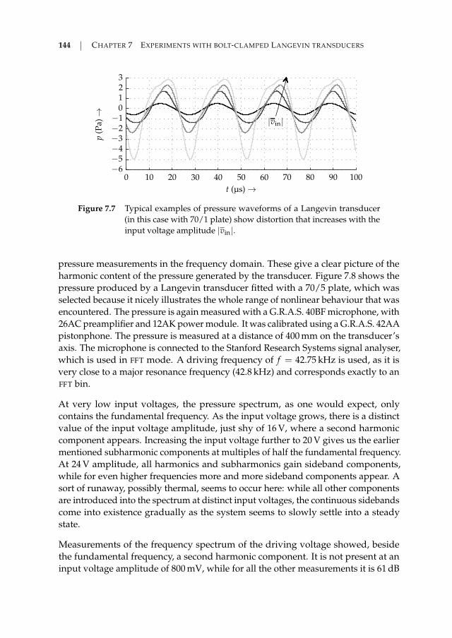
144 CHAPTER 7 EXPERIMENTS WITH BOLT-CLAMPED LANGEVIN TRANSDUCERS
p(P
a)→
t (µs) →
|vin|
0 10 20 30 40 50 60 70 80 90 100−6
−5
−4
−3
−2
−1
0
1
2
3
Figure 7.7 Typical examples of pressure waveforms of a Langevin transducer(in this case with 70/1 plate) show distortion that increases with theinput voltage amplitude |vin|.
pressure measurements in the frequency domain. These give a clear picture of theharmonic content of the pressure generated by the transducer. Figure 7.8 shows thepressure produced by a Langevin transducer fitted with a 70/5 plate, which wasselected because it nicely illustrates the whole range of nonlinear behaviour that wasencountered. The pressure is again measured with a G.R.A.S. 40BF microphone, with26AC preamplifier and 12AK power module. It was calibrated using a G.R.A.S. 42AApistonphone. The pressure is measured at a distance of 400 mm on the transducer’saxis. The microphone is connected to the Stanford Research Systems signal analyser,which is used in FFT mode. A driving frequency of f = 42.75 kHz is used, as it isvery close to a major resonance frequency (42.8 kHz) and corresponds exactly to anFFT bin.
At very low input voltages, the pressure spectrum, as one would expect, onlycontains the fundamental frequency. As the input voltage grows, there is a distinctvalue of the input voltage amplitude, just shy of 16 V, where a second harmoniccomponent appears. Increasing the input voltage further to 20 V gives us the earliermentioned subharmonic components at multiples of half the fundamental frequency.At 24 V amplitude, all harmonics and subharmonics gain sideband components,while for even higher frequencies more and more sideband components appear. Asort of runaway, possibly thermal, seems to occur here: while all other componentsare introduced into the spectrum at distinct input voltages, the continuous sidebandscome into existence gradually as the system seems to slowly settle into a steadystate.
Measurements of the frequency spectrum of the driving voltage showed, besidethe fundamental frequency, a second harmonic component. It is not present at aninput voltage amplitude of 800 mV, while for all the other measurements it is 61 dB
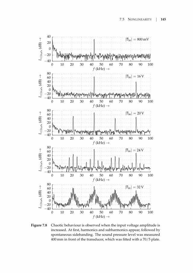
7.5 NONLINEARITY 145
Lp /
20
µP
a(d
B)→
f (kHz) →
Lp /
20
µP
a(d
B)→
f (kHz) →
Lp /
20
µP
a(d
B)→
f (kHz) →
Lp /
20
µP
a(d
B)→
f (kHz) →
Lp /
20
µP
a(d
B)→
f (kHz) →
|vin| = 32 V
|vin| = 24 V
|vin| = 20 V
|vin| = 16 V
|vin| = 800 mV
0 10 20 30 40 50 60 70 80 90 100
0 10 20 30 40 50 60 70 80 90 100
0 10 20 30 40 50 60 70 80 90 100
0 10 20 30 40 50 60 70 80 90 100
0 10 20 30 40 50 60 70 80 90 100
−40−20
020406080
−40−20
020406080
−40−20
020406080
−40−20
020406080
−40
−20
0
20
40
Figure 7.8 Chaotic behaviour is observed when the input voltage amplitude isincreased. At first, harmonics and subharmonics appear, followed byspontaneous sidebanding. The sound pressure level was measured400 mm in front of the transducer, which was fitted with a 70/5 plate.

146 CHAPTER 7 EXPERIMENTS WITH BOLT-CLAMPED LANGEVIN TRANSDUCERS
to 68 dB smaller than the first harmonic component. Moreover, none of the otherharmonic components in figure 7.8 are visible in the input voltage spectrum. It cantherefore be concluded that the distortion is not introduced by the driving amplifier.
The behaviour that figure 7.8 shows, including subharmonics and spontaneoussidebanding, is sometimes encountered in loudspeakers [14, 29, 86, 95, 129]. Judgingfrom publications on the topic, it seems that it is most commonly encountered intraditional voice coil topologies, where it is often attributed to nonlinearity of com-pliance components, although sometimes bending waves in the cone are mentionedas a cause. These nonlinearities introduce chaotic behaviour into the system, suchas witnessed by the measurements that are shown here. It is therefore reasonableto assume that the nonlinearities are introduced by the transducer, especially sincethey also occur in the transducers without plates. It seems that the addition of theradiating plates only amplifies the effect. A first hypothesis is that the nonlinearbehaviour is caused by the transducer’s clamping bolt, which has the effect of anonlinear compliance term due to its prestress.
7.6 Energy transfer
Since the plates do not have the desired effect, the energy transfer is henceforthinvestigated using bare Langevin transducers without any plates attached. Energytransfer measurements are carried out to investigate the dependency of the powertransfer on the distance as well as the input voltage. The transducers that are used forthe remaining experiments were cherry-picked to obtain the largest output power.
7.6.1 Variation of distance
One of the interesting features of a contactless energy transfer system, is how itperforms when the distance changes. Therefore similar measurements as in figure7.6 were performed, but now for a larger distance range. The measurement setup isexactly the same, apart from the different transducers that are used. Measurementsare complicated by the nonlinearity of the transducers, necessitating the use of a lowinput voltage. The normalised power is therefore measured. This allows the resultsto be extrapolated to predict the energy transfer capabilities of similar transducersthat are designed to have a linear response. Because of the low input voltage, themethod of power measurement described in section 7.4 can be used.
The measured output power and efficiency are depicted in figure 7.9 as a function ofthe driving frequency f and the distance zd between the transducers. The maximum

7.6 ENERGY TRANSFER 147
Πo
ut /
|vin|2
(µW
V−
2)
f (kHz)
zd (mm)
0 5 10 15 20 25 30 35 40 40.2
40.3
40.4
40.5
0
10
20
30
40
50
60
70
80
(a)
η(−
)
f (kHz)
zd (mm)
×10−3
0 5 10 15 20 25 30 35 40 40.2
40.3
40.4
40.5
0
1
2
3
4
5
(b)
Figure 7.9 The measured output power Πout (a) and efficiency η (b) decreaserapidly as the distance increases. The resolution in zd is 100 µm in aband of 500 µm around peaks. The resolution elsewhere is reduced to500 µm to enhance the graphs’ clarity.
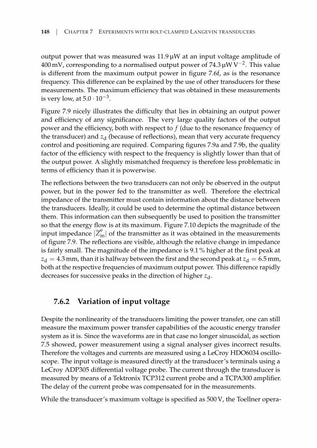
148 CHAPTER 7 EXPERIMENTS WITH BOLT-CLAMPED LANGEVIN TRANSDUCERS
output power that was measured was 11.9 µW at an input voltage amplitude of400 mV, corresponding to a normalised output power of 74.3 µW V−2. This valueis different from the maximum output power in figure 7.6f, as is the resonancefrequency. This difference can be explained by the use of other transducers for thesemeasurements. The maximum efficiency that was obtained in these measurementsis very low, at 5.0 · 10−3.
Figure 7.9 nicely illustrates the difficulty that lies in obtaining an output powerand efficiency of any significance. The very large quality factors of the outputpower and the efficiency, both with respect to f (due to the resonance frequency ofthe transducer) and zd (because of reflections), mean that very accurate frequencycontrol and positioning are required. Comparing figures 7.9a and 7.9b, the qualityfactor of the efficiency with respect to the frequency is slightly lower than that ofthe output power. A slightly mismatched frequency is therefore less problematic interms of efficiency than it is powerwise.
The reflections between the two transducers can not only be observed in the outputpower, but in the power fed to the transmitter as well. Therefore the electricalimpedance of the transmitter must contain information about the distance betweenthe transducers. Ideally, it could be used to determine the optimal distance betweenthem. This information can then subsequently be used to position the transmitterso that the energy flow is at its maximum. Figure 7.10 depicts the magnitude of theinput impedance |Ze
in| of the transmitter as it was obtained in the measurementsof figure 7.9. The reflections are visible, although the relative change in impedanceis fairly small. The magnitude of the impedance is 9.1 % higher at the first peak atzd = 4.3 mm, than it is halfway between the first and the second peak at zd = 6.5 mm,both at the respective frequencies of maximum output power. This difference rapidlydecreases for successive peaks in the direction of higher zd.
7.6.2 Variation of input voltage
Despite the nonlinearity of the transducers limiting the power transfer, one can stillmeasure the maximum power transfer capabilities of the acoustic energy transfersystem as it is. Since the waveforms are in that case no longer sinusoidal, as section7.5 showed, power measurement using a signal analyser gives incorrect results.Therefore the voltages and currents are measured using a LeCroy HDO6034 oscillo-scope. The input voltage is measured directly at the transducer’s terminals using aLeCroy ADP305 differential voltage probe. The current through the transducer ismeasured by means of a Tektronix TCP312 current probe and a TCPA300 amplifier.The delay of the current probe was compensated for in the measurements.
While the transducer’s maximum voltage is specified as 500 V, the Toellner opera-
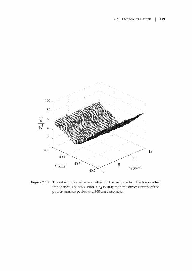
7.6 ENERGY TRANSFER 149
∣ ∣ ∣
Ze in
∣ ∣ ∣
(Ω)
f (kHz) zd (mm)0
5
10
15
40.2
40.3
40.4
40.50
20
40
60
80
100
Figure 7.10 The reflections also have an effect on the magnitude of the transmitterimpedance. The resolution in zd is 100 µm in the direct vicinity of thepower transfer peaks, and 300 µm elsewhere.
150 CHAPTER 7 EXPERIMENTS WITH BOLT-CLAMPED LANGEVIN TRANSDUCERS
tional amplifier that drives it limits the voltage amplitude to 40 V. A transformer istherefore used to boost the input voltage to a maximum of 190 V.
The input power is calculated as the cyclic mean of the product of vin and iin. Theoutput power is obtained from the RMS (root-mean-square) value of vout and theload resistance. Contrarily to previous measurements, the cyclic mean and RMS
value are determined in MATLAB, utilising the autocorrelation to find each signal’speriod.
Measuring at higher power levels means that the transducers heat up throughdissipation. It became clear during measurements that this influences the resonancefrequency of the system and the optimal distance between the transducers, as wellas significantly decreases the output power. The system seems to reach a steadystate after a while. It is likely that this is caused by the thermal characteristics ofthe transducers. A changing resonance frequency is a known nonlinear effect inpiezoelectric materials, that is often attributed to large mechanical deformationsand self-heating [8]. To limit the influence of self-heating as much as possible,measurements are done in short bursts.
The energy transfer is measured for different values of the input voltage amplitude.The measured output power and efficiency are shown in figure 7.11. The optimalfrequency and distance were determined for each value of input voltage to reduce theinfluence of temperature, and possibly other nonlinear effects, as much as possible.The burst mode measurements seemed to help in this respect as the optimal distance,unlike for continuous measurements, was constant at zd = 4.340 mm. The optimalfrequency varied very slightly between 40.346 kHz and 40.354 kHz.
Figure 7.11a shows that the output power has a bending point around |vin| = 50 V,after which the output power increases approximately linearly. In a linear systemone would expect the output power to increase quadratically with the input voltageamplitude. The efficiency in figure 7.11b initially drops very rapidly as the inputvoltage increases, but then falls off at an increasingly slower pace. Whether itreaches a steady state or not can unfortunately not be concluded from this graph.The maximum output power that was measured is 36.3 mW at an input voltageamplitude of 190 V.
7.7 Reproducibility
The reproducibility of the described measurements is a cause for concern, just as itwas in previous chapters. It is investigated here based on the electrical impedance
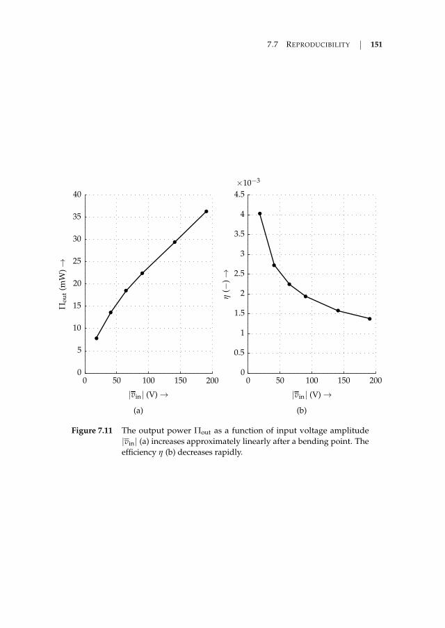
7.7 REPRODUCIBILITY 151
Πo
ut
(mW
)→
|vin| (V) →
0 50 100 150 2000
5
10
15
20
25
30
35
40
(a)
η(−
)→
|vin| (V) →
0 50 100 150 200
×10−3
0
0.5
1
1.5
2
2.5
3
3.5
4
4.5
(b)
Figure 7.11 The output power Πout as a function of input voltage amplitude|vin| (a) increases approximately linearly after a bending point. Theefficiency η (b) decreases rapidly.
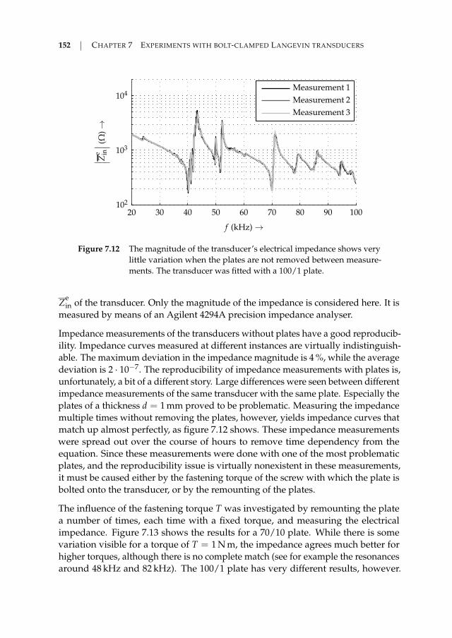
152 CHAPTER 7 EXPERIMENTS WITH BOLT-CLAMPED LANGEVIN TRANSDUCERS
Measurement 3
Measurement 2
Measurement 1∣ ∣ ∣Z
e in
∣ ∣ ∣(Ω
)→
f (kHz) →
20 30 40 50 60 70 80 90 100102
103
104
Figure 7.12 The magnitude of the transducer’s electrical impedance shows verylittle variation when the plates are not removed between measure-ments. The transducer was fitted with a 100/1 plate.
Zein of the transducer. Only the magnitude of the impedance is considered here. It is
measured by means of an Agilent 4294A precision impedance analyser.
Impedance measurements of the transducers without plates have a good reproducib-ility. Impedance curves measured at different instances are virtually indistinguish-able. The maximum deviation in the impedance magnitude is 4 %, while the averagedeviation is 2 · 10−7. The reproducibility of impedance measurements with plates is,unfortunately, a bit of a different story. Large differences were seen between differentimpedance measurements of the same transducer with the same plate. Especially theplates of a thickness d = 1 mm proved to be problematic. Measuring the impedancemultiple times without removing the plates, however, yields impedance curves thatmatch up almost perfectly, as figure 7.12 shows. These impedance measurementswere spread out over the course of hours to remove time dependency from theequation. Since these measurements were done with one of the most problematicplates, and the reproducibility issue is virtually nonexistent in these measurements,it must be caused either by the fastening torque of the screw with which the plate isbolted onto the transducer, or by the remounting of the plates.
The influence of the fastening torque T was investigated by remounting the platea number of times, each time with a fixed torque, and measuring the electricalimpedance. Figure 7.13 shows the results for a 70/10 plate. While there is somevariation visible for a torque of T = 1 N m, the impedance agrees much better forhigher torques, although there is no complete match (see for example the resonancesaround 48 kHz and 82 kHz). The 100/1 plate has very different results, however.
7.8 CONCLUSIONS AND DISCUSSION 153
Figure 7.14 depicts the impedance for the same three fastening torques. While theresults match to some extent for T = 1 N m, the variation is drastically higher forhigher torques. Many new resonances appear, and some move to another frequency.
Since the impedance measurements do not necessarily agree better when the platesare fixed with an equal torque, the problems regarding reproducibility must becaused by variation in the positioning of the plates. It turned out that the platesof 1 mm thickness are thin enough to move laterally in the thread of the screwthat should hold them in place. The plate is therefore not automatically centredby the screw. This can easily result in very different behaviour, as it makes thetransducer asymmetric. Possibly the 70/10 plates are centred better when the torqueis increased, which would explain the greater consistency in results for higherfastening torques. At 1 N m both plates are very comparable. This is to be expected,as they are quite loosely attached to the transducer, so there is probably a reducedinfluence of the radiating plate.
The point to take away from this is that reassembly of the transducers is gener-ally a cause of variation in measurement results, especially for thin plates. Allmeasurement results given in this chapter are therefore a possible set of outcomes.This variation is only increased by the temperature dependency that was alreadydiscussed in section 7.6.2. It also shows that modelling of this system for designpurposes would not have been very meaningful, as the behaviour in reality maybe very different due to reproducibility issues, even if an initial model would showgood agreement with measurement results.
7.8 Conclusions and discussion
This chapter set out to investigate impedance adaptation of transducers throughenlargement of their radiating surface, in an attempt to reduce reflections, andparticularly to increase the output power. Plates of varying radius and thickness thatare attached to the transducers were chosen as a solution. Bolt-clamped Langevintransducers were chosen for their large power handling capabilities and their highefficiency. Unfortunately, initial voltage gain measurements indicated that the platesdo not increase the output power. These measurements suggest that the largest partof the power is transferred between the centres of the transducers, and not betweenthe plate surfaces.
A subsequent set of energy transfer measurements proves that the plates indeed donot increase the output power; the highest output power was obtained without theuse of plates. Although the output power is lower for every plate size, the energy

154 CHAPTER 7 EXPERIMENTS WITH BOLT-CLAMPED LANGEVIN TRANSDUCERS
∣ ∣ ∣
Ze in
∣ ∣ ∣
(Ω)→
f (kHz) →
∣ ∣ ∣Z
e in
∣ ∣ ∣(Ω
)→
f (kHz) →
∣ ∣ ∣
Ze in
∣ ∣ ∣
(Ω)→
f (kHz) →
T = 4 N m
T = 2.5 N m
T = 1 N m
20 30 40 50 60 70 80 90 100
20 30 40 50 60 70 80 90 100
20 30 40 50 60 70 80 90 100
102
103
104
102
103
104
102
103
104
Figure 7.13 Measurements of the magnitude of the transducer impedance showthe variation that occurs in remounting the plates. The 70/10 platethat is used for these experiments is fastened with a fixed torque of1 N m, 2.5 N m or 4 N m.

7.8 CONCLUSIONS AND DISCUSSION 155
∣ ∣ ∣
Ze in
∣ ∣ ∣
(Ω)→
f (kHz) →
∣ ∣ ∣Z
e in
∣ ∣ ∣(Ω
)→
f (kHz) →
∣ ∣ ∣
Ze in
∣ ∣ ∣
(Ω)→
f (kHz) →
T = 4 N m
T = 2.5 N m
T = 1 N m
20 30 40 50 60 70 80 90 100
20 30 40 50 60 70 80 90 100
20 30 40 50 60 70 80 90 100
102
103
104
102
103
104
102
103
104
Figure 7.14 The 100/1 plates are subject to much more variation, judging fromthe transducer impedance. The screw attaching the plate to thetransducer is again fastened with a torque of 1 N m, 2.5 N m or 4 N m.
156 CHAPTER 7 EXPERIMENTS WITH BOLT-CLAMPED LANGEVIN TRANSDUCERS
transfer efficiency is slightly higher with the 40/10 plates attached. This is due to asmaller net distance between the transmitter and the receiver (2 mm, compared to4.5 mm without plates), because of the discs that clamp the plates to the transducers.
The unsatisfying performance of the radiating plates as impedance matching devicesis ascribed to the normal vibration modes of the plates. These result in a partitioningof the plates into small sections that vibrate with opposite phase, causing an acousticshort circuit that severely reduces the radiated power. At high frequencies it is verydifficult to prevent these normal modes. It is possible, however, to use plates havinglocal thickness variations, which negate the phase difference that the normal modesintroduce.
Matters are complicated further by the nonlinearity of the transducers. It causestheir performance at high power levels to significantly deviate from the expec-ted sinusoidal behaviour. Harmonics and subharmonics appear at discrete inputvoltage amplitudes, and at a certain point spontaneous sidebanding occurs, indic-ating chaotic behaviour. The same phenomena have been observed in voice coilloudspeakers. Normally they are blamed on nonlinearity of the compliance of theloudspeaker suspension, or on diaphragm modes. It is possible that they are intro-duced in this AET system because of nonlinearity of the materials, or because of thepretension applied by the transducer’s prestress bolt.
Because of the nonlinear behaviour, low power measurements of the energy transferwere done initially. The maximum output power that was measured is 12 µW at aninput voltage amplitude of 400 mV. Extrapolation to a voltage of 500 V, which isthe maximum voltage that the transducers allow, would yield an output power ofΠout = 18.6 W. Naturally, linearity of both the transducer and the air are assumed.The maximum efficiency that was attained in these measurements is 5 · 10−3. Thislow value is a consequence of the very poor impedance matching of the transducersto the medium.
The measurements again illustrate the stringent requirements on the positioningof the transducers imposed by the reflections. The high quality factor that thereflections bring to the system means that a 100 µm displacement is accompaniedby a 7 dB drop in output power. Therefore accurate positioning of the transducersis of paramount importance. If an AET system is to transfer any energy, it will benecessary to adjust the position of the transmitter depending on the location of thereceiver. Since the distance between consecutive peaks is 4.3 mm for this system (cf.figure 7.9), a maximum variation of the transmitter position of 2.2 mm is required,which is quite acceptable. Information about the optimum position of the transmittercan possibly be obtained from the transmitter impedance, since it gives informationabout the location of the energy transfer peak. The difference in impedance betweenan output power maximum and minimum is 9 % at the first peak, making it quite

7.8 CONCLUSIONS AND DISCUSSION 157
discernible, but for larger zd it is barely detectable.
Measurements of the variation of the output power with input voltage revealedan approximately linear relation between the two for high values of input voltage,instead of the expected quadratic relationship. Consequently, the efficiency η de-creases rapidly for higher input voltages. The maximum obtained output power is36.3 mW at 190 V input voltage amplitude. From the measured normalised outputpower in figure 7.9a, one would have expected an output power of 2.7 W.
The reproducibility of measurement results was judged based on electrical imped-ance measurements of the transducers. While the reproducibility of these measure-ments was excellent when the bare transducers were measured, much variation wasobserved when radiating plates were attached to them. It was deduced throughexperiments that the most likely cause of this variation is the positioning of theplates with respect to the transducer. The problem seemed to be most prevalent withthe plates of 1 mm thickness. These proved difficult to position symmetrically withrespect to the axis of the transducer, causing many varying resonances.
Lastly, the experiments in this chapter show that the frequency of optimal powertransfer varies not only with distance, but also with ambient temperature. It istherefore important to perform measurements both as a function of distance andfrequency. Alternatively, a maximum power tracking algorithm can be used, so thatthe system always works at its optimal frequency.


CH
AP
TE
R
8 Conclusions &recommendations
THIS THESIS focuses on the contactless transfer of energy from an electricalsource to an electrical load, using sound waves that propagate through air as anintermediate energy carrier. Its main purpose lies in providing an exploratory
overview of the subject, pointing out the features, opportunities and limitations ofthe approach. It investigates a number of peculiarities of the system and describesvarious paths that have been followed in the pursuit of optimised system perform-ance. While the research has answered several questions, it has simultaneouslyraised numerous new ones, paving the way—and leaving a couple of directionsigns—for further investigation.
This final chapter briefly summarises the most important conclusions of the workthat has been presented in this dissertation. Furthermore, it lists the main contribu-tions of the research, and discusses several recommendations for future work onacoustic energy transfer in air. AET being a quite new field, this list naturally is farfrom exhaustive.
8.1 Conclusions
A theoretical limit to the efficiency of acoustic energy transfer has been derived,based on a model that includes diffraction, attenuation and transducer losses. Themodel indicates that, for a maximum transmitter and receiver diameter of 20 cmand 1 m distance between the two, acoustic energy transfer has the potential to
159

160 CHAPTER 8 CONCLUSIONS & RECOMMENDATIONS
perform at least 5 to 10 times better than an inductively coupled system of the samedimensions. Optimal electrical loading conditions were derived from this model,which indicate that the receiving element, unfortunately, has an efficiency of 50 %when maximum output power is desired.
The model on which the theoretical limit is based was validated through experiments,showing that energy transfer by means of sound waves is feasible. A maximumoutput power of 40 mW was demonstrated using piezoelectric transducers. In thiscase, the output power was limited by the mechanical breakdown of the transmittingtransducer. The measurements revealed the occurrence, influence and importanceof reflections. These create periodic maxima and minima of energy transfer andefficiency, spaced at half-wavelength intervals, and thus restrict the free placementof a receiving element. Transducer losses were identified from impedance measure-ments in vacuum, to allow a fair comparison between the measurements and themodel. The measured efficiency corresponds very well to the theoretical limit at thefirst spatial resonance peak, but the decline in efficiency with the distance betweenboth transducers proved to be greater in reality than predicted by the model. Thisis most likely due to the pressure and particle velocity distribution being altereddrastically by the reflections.
Reflections have been modelled both analytically and numerically. The analyticalmodel is based on a transmission line model, assuming plane waves. A lumpedelement attenuation coefficient accounts for the spreading of sound waves and theabsorption in the medium. It is obtained from a circular piston radiator model anddepends on the spatial coordinate. Because there are unknowns in the transducermodel, parameter fitting is used to bring the model into line with measurement data.Results show a very good agreement between the two, but the obtained transducerparameters are nonphysical. Nevertheless, the results show that the model is notwithout merits. It is expected that simulation results deviate for distances that lie inthe near field of the transducer, due to averaging of the pressure in this region in thecalculation of the attenuation constant.
The numerical model describes reflections by means of multiphysical finite elementanalysis of the transducers in an air domain. Although it is able to predict the effectof reflections on the output power and efficiency, it is unable to do so accurately.The predicted output power is an order of magnitude too high and the variationof the input power with the distance between the two transducers is considerablydifferent from the measurements. This is attributed to an incorrect model of thetransducers. Sensitivity analysis identified the most influential parameters, butrevealed no extreme sensitivity to changes in their values.
Stepped-exponential horns were designed, optimised and constructed as a means ofimpedance adaptation for both the transmitting and receiving transducers. Their
8.2 THESIS CONTRIBUTIONS 161
profile is comprised of a stepwise change in radius followed by a section that flaresout exponentially. Resonance in the horn is used to greatly increase its throatimpedance. The horns improved the output power by a factor 3.1, and the efficiencyby a factor 7.5 at 10 cm distance between the transmitter and the receiver. Theexperimental results deviate significantly from the finite element model that wasused for their optimisation. This discrepancy is likely caused by a combination oftemperature variation, which detunes the horn’s resonance frequency, an unknownpiezoelectric material and component variation of the transducers. The exact profileof the flaring section was shown to be irrelevant for the output pressure.
Radiating surface enlargement has been investigated as a second means of imped-ance adaptation. It was applied to bolt-clamped Langevin transducers in the formof aluminium plates that are screwed onto the transducer. Nine different plate sizeswere manufactured to investigate the influence of the plate dimensions. It was foundthat the plates do not increase the output power. This is due to their normal modes,which severely reduce the effective velocity of the radiator. Moreover, the trans-ducers suffer from nonlinear behaviour, manifesting in harmonics, subharmonicsand spontaneous sidebanding when the driving voltage is increased. Furthermore,problems were encountered with respect to reproducibility due to difficulty incoaxial placement of plates on transducers. The maximum output power that wasmeasured (without plates), is 36.3 mW. Measurements showed the importance ofmeasuring as a function of the frequency and the distance between the transducers.It was found that optimal positioning of the transmitter is possible based on itselectrical impedance.
Essentially, acoustic energy transfer through air is possible. Achieved power levelsare adequate for small systems such as sensors, MEMS, et cetera, but are insufficientfor implementation in more power hungry applications such as actuators or wire-less charging. The transducers are the restricting factor. Proposed models of AET
are usable, but they require more research to become accurate enough for designpurposes. Throughout this thesis, transducer modelling has been shown to be ofcritical importance for accurate acoustic energy transfer modelling, since it is theelement that connects the electrical, mechanical and acoustic domains. Almost alluncertainty in models can ultimately be traced down to the transducer.
8.2 Thesis contributions
• Introduction to a broader audience of acoustic energy transfer as a methodof contactless transfer of electrical energy. Contactless energy transfer bymeans of sound waves was already introduced in its most basic form in

162 CHAPTER 8 CONCLUSIONS & RECOMMENDATIONS
1985 [19]. Unfortunately, it was never picked up as a serious contender toelectromagnetic alternatives. The research done for this thesis and publica-tions thereof have helped in bringing the subject to the attention of a broaderaudience [97].
• Experimental validation of the principle of contactless energy transfer em-ploying vibration of air as a means of energy transport. Viability of theprinciple of AET has been shown through measurements of the electrical en-ergy transfer by means of sound waves on a number of setups. A maximumelectrical output power of 40 mW has been achieved.
• Derivation of a theoretical upper limit to acoustic energy transfer efficiencyA theoretical limit to the efficiency of acoustic energy transfer has been derived.It is based on an analytical model of the energy transfer between two circulartransducers, describing diffraction and attenuation losses. The losses in thetransducers were estimated from their equivalent electrical circuits. Optimalloading conditions for the receiving transducer have been derived.
• Analytically and numerically modelling the reflections that occur in an AET
system. Reflections have been shown to be a very essential characteristic ofa typical acoustic energy transfer system. They generate a partial standingwave that restricts the placement of the receiver to distinct locations wherethe energy transfer and efficiency are high. Reflections are therefore of largeinfluence on the energy transfer. This thesis presents two models of reflections:one based on transmission line theory, and the other a finite element model.
• Design and optimisation of impedance adaptation measures. Impedancemismatch has been identified as a major factor limiting the performance of anacoustic energy transfer setup. At the receiving side it introduces reflections,thereby limiting the absorbed power and introducing more losses, while amismatch at the transmitting end limits the power transfer to the medium.Two methods of impedance adaptation have been investigated:
– Resonant horn structures, comprising a stepwise change in radius fol-lowed by an exponentially varying radius profile. Horns have been de-signed and optimised for both the transmitting and receiving transducers.The energy transfer using these horns has been verified experimentally.
– Acoustic impedance transformation for bolt-clamped Langevin trans-ducers, consisting of aluminium plates of varying radius and thickness.A setup was built and measurements were done to verify the influenceof the plates on the energy transfer, as well as identifying various ef-fects that limit the energy transfer, i.e. nonlinearity and chaos, thermalcharacteristics and normal vibration modes.
8.3 RECOMMENDATIONS 163
8.3 Recommendations
No research is ever complete, unfortunately, and there is always room for improve-ment. Especially in a subject that is in its infancy, such as acoustic energy transfer,there is bound to be many a topic left untouched. Many ideas about new researchdirections, or how to improve results that have been obtained have formed duringthe course of the research. The most important recommendations are discussed inthis section. Some of these have already been treated in the concerning chapters ofthis dissertation, but they will be repeated here for the sake of completeness.
Modelling The models that have been presented in this thesis show many sim-ilarities with measurements, but generally they are unable to accurately predict thebehaviour of the AET systems. A major factor in this respect is the validation of theseparate parts of the model. For example, the transmission line model cannot bevalidated properly because the transducer model contains too many uncertainties. Itis therefore advisable to construct models of the separate parts of the system (trans-ducer, wave propagation, reflections), and validate them separately. Once they arefound to be accurate enough the system model can be assembled and validated as awhole. In this thesis it was attempted to validate all models through measurementsof electrical quantities only. It will be necessary to also measure mechanical quant-ities for proper validation. One can think of pressure measurements, or velocityprofile estimation (for example by means of acoustic holography [4, 42, 83]).
Especially for the purpose of accurately modelling acoustic energy transfer, oneshould start with acoustic energy in its most basic form. Problematic factors shouldbe eliminated as much as possible from the system, so that the basic mechanismscan be thoroughly researched and understood. One can think of circumventing theproblem of reflections using a very small receiver, so that waves diffract around itand reflections are negligible. Other possibilities are using transducers that are suffi-ciently rigid, or do not vibrate at their normal modes but rather can be consideredone-dimensional. This greatly facilitates their modelling and the complexity of theircoupling with the medium. A last example is acoustic energy transfer through awave guide, so that spreading losses can be taken out of the equation. Some of thesechoices will probably reduce the power level and efficiency, but will allow one tofully understand the system, and from there make choices about how to optimise it.
Transducers Transducer design for acoustic energy transfer is a whole field ofresearch in itself, or should at least become one in near future. All experiments inthis dissertation made use of piezoelectric transducers, and not only this thesis; theuse of piezoelectric transducers is prevalent throughout the field of acoustic energytransfer. The only example to date of the use of another type of actuator for AET

164 CHAPTER 8 CONCLUSIONS & RECOMMENDATIONS
is [43], where an electromagnetic acoustic transducer (EMAT) design is evaluated.The authors concluded that piezoelectric transducers are better suited, under therestriction that they are well coupled to the medium. There is, however, no reasonnot to consider other actuator topologies, such as voice coil or ribbon loudspeakers,electrostatic topologies, magnetostrictive materials, et cetera. The advantage ofpiezoelectric materials is that they can be used at very high frequencies and highefficiencies. The frequencies used in this research however, are not extremely high(up to 40 kHz). Therefore, different transducer designs may be just as efficient. Theycan circumvent specific problems of piezoelectric components, such as having to usethem at their resonance frequency for any output of significance. This thesis showsthat these high quality factor resonances can be very problematic when they have tobe matched.
During the research it gradually became clear that impedance matching is not by faras important for the transmitter as it is for the receiver. The underlying problem isdepicted graphically in figure 8.1 for a set of bolt-clamped Langevin transducers. Apoorly matched transducer implies a reflection coefficient close to one, and a verysmall transmission coefficient. A wave that arrives at the radiating surface of thetransmitter mostly reflects, and only part is transmitted to the air, illustrated bythe length of the arrows in figure 8.1. The reflected wave, however, stays confinedto the geometry of the transducer. It will reflect from the back of the transducerand return to the radiating face. This is the resonance condition on the basis ofwhich bolt-clamped Langevin transducers work. These reflections do not causelosses per se, as long as the material is relatively lossless. The wave that arrivesat the surface of the receiver, on the other hand, mostly reflects off it, and only asmall part continues as a stress wave in the transducer. The reflections from thereceiver travel back to the transmitter, where they reflect again; A process that wasamply discussed in chapter 5. As long as the directivity of the transducers is high,this will not cause severe losses, but as soon as diffraction comes into play, theefficiency degrades considerably due to spreading of the reflected wave. This showsthat the impedance adaptation of the receiver is much more important than that ofthe transmitter. A very light receiver, such as a ribbon transducer or electrostaticloudspeaker, will be much more appropriate than a piezoelectric transducer in thiscase. This also illustrates that optimal designs for the transmitter and reducer mayconsist of entirely different topologies. The transmitter design should be focused ondelivering high power, while the receiver design should focus on a low impedancetransducer.
Besides a low impedance, the receiver will have to adhere to a specific design.Suppose a plane wave propagates towards a receiver, as in figure 8.2. Ideally, theratio between the pressure p1 and particle velocity u1 at the face of the receiver isequal to Za
0 , so that the wave does not reflect. If the receiver is much thinner than a
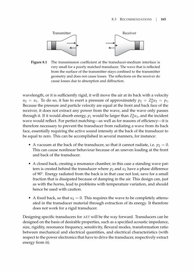
8.3 RECOMMENDATIONS 165
Transmitter Receiver
Figure 8.1 The transmission coefficient at the transducer-medium interface isvery small for a poorly matched transducer. The wave that is reflectedfrom the surface of the transmitter stays confined to the transmittergeometry and does not cause losses. The reflections on the receiver docause losses due to absorption and diffraction.
wavelength, or it is sufficiently rigid, it will move the air at its back with a velocityu2 = u1. To do so, it has to exert a pressure of approximately p2 = Za
0u2 = p1.Because the pressure and particle velocity are equal at the front and back face of thereceiver, it does not extract any power from the wave, and the wave only passesthrough it. If it would absorb energy, p1 would be larger than Za
0u1, and the incidentwave would reflect. For perfect matching—as well as for reasons of efficiency—it istherefore necessary to prevent the transducer from radiating a wave from its backface, essentially requiring the active sound intensity at the back of the transducer tobe equal to zero. This can be accomplished in several manners, for instance:
• A vacuum at the back of the transducer, so that it cannot radiate, i.e. p2 = 0.This can cause nonlinear behaviour because of an uneven loading at the frontand back of the transducer.
• A closed back, creating a resonance chamber; in this case a standing wave pat-tern is created behind the transducer where p2 and u2 have a phase differenceof 90°. Energy radiated from the back is in that case not lost, save for a smallfraction that is dissipated because of damping in the air. This design can, justas with the horns, lead to problems with temperature variation, and shouldhence be used with caution.
• A fixed back, so that u2 = 0. This requires the wave to be completely attenu-ated in the transducer material through extraction of its energy. It thereforedoes not work for a rigid transducer.
Designing specific transducers for AET will be the way forward. Transducers can bedesigned on the basis of desirable properties, such as a specified acoustic impedance,size, rigidity, resonance frequency, sensitivity, flexural modes, transformation ratiobetween mechanical and electrical quantities, and electrical characteristics (withrespect to the power electronics that have to drive the transducer, respectively extractenergy from it).
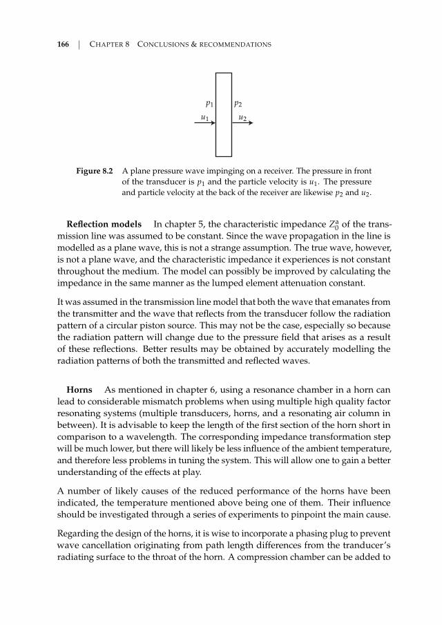
166 CHAPTER 8 CONCLUSIONS & RECOMMENDATIONS
p2p1
u1 u2
Figure 8.2 A plane pressure wave impinging on a receiver. The pressure in frontof the transducer is p1 and the particle velocity is u1. The pressureand particle velocity at the back of the receiver are likewise p2 and u2.
Reflection models In chapter 5, the characteristic impedance Za0 of the trans-
mission line was assumed to be constant. Since the wave propagation in the line ismodelled as a plane wave, this is not a strange assumption. The true wave, however,is not a plane wave, and the characteristic impedance it experiences is not constantthroughout the medium. The model can possibly be improved by calculating theimpedance in the same manner as the lumped element attenuation constant.
It was assumed in the transmission line model that both the wave that emanates fromthe transmitter and the wave that reflects from the transducer follow the radiationpattern of a circular piston source. This may not be the case, especially so becausethe radiation pattern will change due to the pressure field that arises as a resultof these reflections. Better results may be obtained by accurately modelling theradiation patterns of both the transmitted and reflected waves.
Horns As mentioned in chapter 6, using a resonance chamber in a horn canlead to considerable mismatch problems when using multiple high quality factorresonating systems (multiple transducers, horns, and a resonating air column inbetween). It is advisable to keep the length of the first section of the horn short incomparison to a wavelength. The corresponding impedance transformation stepwill be much lower, but there will likely be less influence of the ambient temperature,and therefore less problems in tuning the system. This will allow one to gain a betterunderstanding of the effects at play.
A number of likely causes of the reduced performance of the horns have beenindicated, the temperature mentioned above being one of them. Their influenceshould be investigated through a series of experiments to pinpoint the main cause.
Regarding the design of the horns, it is wise to incorporate a phasing plug to preventwave cancellation originating from path length differences from the tranducer’sradiating surface to the throat of the horn. A compression chamber can be added to
8.3 RECOMMENDATIONS 167
the back to increase linearity. Although this has not been found to be a problem, itmay become one when power levels are increased.
Possibly horns can be used advantageously in a hybrid impedance matching topo-logy, where the first step is obtained by means of matching layers, and a secondstep through application of a horn. Matching layers can be used very well forhigh to medium-high impedance steps, but are ill-suited for low impedance media(see section 5.3). Horns, on the other hand, are best used for the medium to lowimpedance step, since they always perform the last step, down to the impedanceof the radiating medium. Using this solution they do not have to bridge the entireimpedance gap between the transducer and the medium.
Diaphragm design Normal modes make radiation from a diaphragm ineffi-cient. They are therefore best avoided. This can be challenging when high fre-quencies and a large radiating surface are amongst the requirements. While inloudspeaker design it is not uncommon to use dissipative diaphragm materials, sothat modes are damped [20], this is not a viable option for acoustic energy transfer,as it adds to the losses of the system. A diaphragm hence must be as rigid as possible.Great improvements over the flat plates that were used in chapter 7 can be obtainedby using a cone shape for example (as is used in loudspeakers), by using a stiffermaterial or by dividing the radiating surface into smaller segments by means ofa transducer array. Alternatively, the flexural modes can be used advantageously,since the transducers operate at a single frequency. Gallego-Juarez et al. designedhigh efficiency, high directivity transducers where a plate of stepped thickness can-cels the phase difference in the radiation due to the plate’s normal modes [11,36–39].These will certainly be useful for AET as a transmitter design.
General considerations Quite a few problems that had to be dealt with duringthis research were linked with finite element analysis. They mostly were causedby high quality factor resonances. A small change in mesh parameters can in sucha case shift the resonance frequency by several Hertz, which can drastically alterthe output of the simulation. Low efficiency systems, such as AET, are also difficultto simulate since the output power can often be of the same order of magnitudeas the error in the simulation. It is therefore advisable to decouple the simulationinto separate parts, e.g. a transmitter, wave propagation and a receiver. This willimprove the accuracy of the simulations. Care should still be taken in matchingdifferent resonance frequencies.
On the same topic, when designing a setup, one should make sure that a resonancefrequency is adjustable, or a lower quality factor should be used. While this pos-sibly comes at the expense of maximum efficiency and output power, when takingcomponent variation and model inaccuracy into account the power transfer and
168 CHAPTER 8 CONCLUSIONS & RECOMMENDATIONS
efficiency will likely be higher.
All acoustic energy transfer systems that were discussed in this thesis sufferedfrom much higher spreading losses than attenuation losses. In such a case it isbeneficial to consider focusing, or diffraction-free beam patterns, as they improvethe directivity of the transmitter. They improve the efficiency, especially for largerdistances. For very high frequencies the effect will be less pronounced, as in that casespreading losses decrease and absorption losses rise. Phased array transducers canbe used to this end, for example capacitive micromachined ultrasonic transducers(CMUT) [67], or piezoelectric transducer arrays such as used in medical ultrasoundapplications [22]. A phased array has the added advantage of beam steering, whichis necessary when the location of the receiver is a priori unknown. For large outputpower one could consider a design consisting of a large surface area filled withsmall transducers. A possible difficulty lies in tuning all transducers to the sameresonance frequency.
One goal of impedance adaptation is to prevent reflections, so that the position ofthe receiver can be chosen freely, instead of being restricted to multiples of half awavelength. If all impedance adaptation measures fail, one can opt to adjust thedistance between both transducers mechanically to obtain the maximum outputpower. The required distance variation is of the order of a couple of millimetres forkilohertz waves, which is easily achieved (4.3 mm at 20 kHz, for instance).
Lastly, measurements should preferably be performed at a constant temperature,since the optimal distance (due to reflections), changes as a function of soundvelocity, and therefore temperature.

AP
PE
ND
IX
A Symbols and notation
A.1 Symbols
Symbol Quantity Unit
A Surface area m2
B Magnetic flux density TB Adiabatic bulk modulus Pac Sound velocity m s−1
Elastic constant Pacp Isobaric mass heat capacity of air J kg−1 K−1
D Electric displacement field C m−2
e Piezoelectric stress constant C m−2 or N V−1 m−1
E Electric field V m−1
f Frequency HzF Force Ni Current AI Instantaneous sound intensity W m−2
k Angular wave number m−1
l Length mm Horn flare constant m−1
p Pressure PaQ Quality factor −
Volume velocity m3 s−1
169

170 APPENDIX A SYMBOLS AND NOTATION
Symbol Quantity Unit
R Reflection coefficient −R The set of real numbers ?S Strain −S Transmitter sensitivity Pa V−1
T Stress Pau Particle velocity m s−1
v Voltage VW Work Jzd Distance between transmitter and receiver mZa Acoustic impedance N s m−3
Ze Electrical impedance ΩZ The set of integers ?α Absorption coefficient m−1
ε Permittivity F m−1
η Energy transfer efficiency −ξ Particle displacement mκ Thermal conductivity W m−1 K−1
λ Wavelength mµ Viscosity kg m−1 s−1
Π Power Wρ Density kg m−3
ω Radial frequency s−1
A.2 Subscripts and superscripts
Subscript Quantity
a Active sound intensityatt Attenuationc Cutoff
dif Diffractione Pertaining to the electrical domainL Loadm Mouth
Pertaining to the mechanical domainp Point sourcer Receivedt Throat
Total

A.3 NOTATION 171
Subscript Quantity
tr Transducerx, y, z Component in x, y or z direction
0 EquilibriumOffsetSource amplitude
Superscript Quantity
a Acoustice ElectricalE Value for constant electric fieldS Value for constant strain
A.3 Notation
Operator Quantity
a Complex representation~a Vectora Unit vector in the direction of~a: a = ~a/‖~a‖
~a ·~b Dot product of vectors~a and~b~a×~b Cross product of vectors~a and~b∇a Gradient of a∇ ·~a Divergence of~a∇×~a Curl of~aRe(a) Real part of aIm(a) Imaginary part of a
a∗ Complex conjugate of a|a| Absolute value of a‖~a‖ Euclidian norm of~a
A.4 Acronyms
Acronym Meaning
AC Alternating currentAET Acoustic energy transfer

172 APPENDIX A SYMBOLS AND NOTATION
Acronym Meaning
BLT Bolt-clamped Langevin transducerCET Contactless energy transfer
CMUT Capacitive micromachined ultrasonic transducer(s)DC Direct currentEM Electromagnetic
EMF Electromotive forceFE Finite element
FFT Fast Fourier transformMEMS Microelectromechanical system(s)
PZT Lead zirconate titanateRF Radio frequency
RMS Root-mean-square
A.5 Physical constants
Constant Value Unit Quantity
c 3.4326 · 102 m s−1 Sound velocity at 20 CcEM 2.9979 · 108 m s−1 Speed of light in vacuumcp 1.005 · 103 J kg−1 K−1 Isobaric mass heat capacity of air at
20 Cp0 1.013 25 · 105 Pa Atmospheric pressureZa
0 4.1332 · 102 rayl Characteristic impedance of air at20 C
γ 1.400 − Ratio of specific heats of airε0 8.8542 · 10−12 F m−1 Permittivity of free spaceκ 0.0257 W m−1 K−1 Thermal conductivity of air at 20 Cµ 1.8369 · 10−5 kg m−1 s−1 Viscosity of air at 20 Cρ0 1.2922 kg m−3 Air density at 0 C
1.2041 kg m−3 Air density at 20 C

AP
PE
ND
IX
B Coordinate systems
B.1 Coordinate transformations
B.1.1 Spherical coordinates
This thesis uses a spherical coordinate system in which the polar angle θ is theangle between the positive z-axis and the vector. The azimuthal angle ϕ is thecounterclockwise angle between the x-axis and the vector’s projection in the xy-plane. By definition r ≥ 0, 0 ≤ θ ≤ π, 0 ≤ ϕ ≤ 2π. The conversion betweenCartesian and spherical coordinates is given by
x = r sin θ cos ϕ , r =√
x2 + y2 + z2 ,
y = r sin θ sin ϕ , θ = arccos( z
r
),
z = r cos θ , ϕ = arctan( y
x
).
B.1.2 Cylindrical coordinates
A point in a cylindrical coordinate system is defined by a radial distance r, a height zand an azimuthal angle ϕ, which is defined in the same manner as for the sphericalcoordinate system. Here again r ≥ 0, 0 ≤ ϕ ≤ 2π, and z ∈ R. The coordinate
173

174 APPENDIX B COORDINATE SYSTEMS
transformation between Cartesian and cylindrical coordinates is given by
x = r cos ϕ , r =√
x2 + y2 ,
y = r sin ϕ , ϕ = arctan( y
x
).
The z-coordinate is equal in both systems.
B.2 Gradient
Let us assume we have a coordinate system with coordinates x1, x2 and x3 andcorresponding unit vectors x1, x2 and x3, in which a function f is defined in a point~x = x1 x1 + x2 x2 + x3 x3. The gradient of f is then according to [51] equal to
∇ f =1h1
d fdx1
x1 +1h2
d fdx2
x2 +1h3
d fdx3
x3 , (B.1)
in which the scale factors h1, h2 and h3 are given by
h1 =
∥∥∥∥ ∂~x∂x1
∥∥∥∥ , h2 =
∥∥∥∥ ∂~x∂x2
∥∥∥∥ , h3 =
∥∥∥∥ ∂~x∂x3
∥∥∥∥ . (B.2)
B.2.1 Gradient in spherical coordinates
Deriving the gradient in spherical coordinates boils down to calculating the scalefactors in (B.2), with x1 = r, x2 = θ and x3 = ϕ. They are easily found from thedefinition of the coordinate transformation in section B.1.1:
h1 =
∥∥∥∥∂~x∂r
∥∥∥∥ = 1 , (B.3a)
h2 =
∥∥∥∥∂~x∂θ
∥∥∥∥ = |r| = r , (B.3b)
h3 =
∥∥∥∥ ∂~x∂ϕ
∥∥∥∥ = |r sin(θ)| = r sin(θ) . (B.3c)
Substituting these coefficients in equation (B.1) results in the definition of the gradi-ent in spherical coordinates:
∇ f =d fdr
r +1r
d fdθ
θ +1
r sin(θ)d fdϕ
ϕ . (B.4)

B.2 GRADIENT 175
B.2.2 Gradient in cylindrical coordinates
The gradient in cylindrical coordinates is found from (B.2) and section B.1.2. Thescale factors are given by
h1 =
∥∥∥∥∂~x∂r
∥∥∥∥ = 1 , (B.5a)
h2 =
∥∥∥∥ ∂~x∂ϕ
∥∥∥∥ = |r| = r , (B.5b)
h3 =
∥∥∥∥∂~x∂z
∥∥∥∥ = 1 . (B.5c)
The gradient is found from these scale factors as
∇ f =d fdr
r +1r
d fdϕ
ϕ +d fdz
z . (B.6)


References
[1] “Tesla’s tower,” New York American, 22 May 1904.
[2] R. M. Aarts, “Optimally sensitive and efficient compact loudspeakers,” Journal of theAcoustical Society of America, vol. 119, no. 2, pp. 890–896, Feb. 2006.
[3] R. M. Aarts and A. J. E. M. Janssen, “Approximation of the Struve function H1 occurringin impedance calculations,” Journal of the Acoustical Society of America, vol. 113, no. 5,pp. 2635–2637, May 2003.
[4] R. M. Aarts and A. J. E. M. Janssen, “Acoustic holography for piston sound radiationwith non-uniform velocity profiles,” in Proceedings of the 17th International Congress onSound & Vibration, Jul. 2010, pp. 1–6.
[5] M. Abramowitz and I. A. Stegun, Eds., Handbook of mathematical functions, 10th ed.Washington D.C.: US Government Printing Office, 1972.
[6] T. E. G. Álvarez-Arenas, “Acoustic impedance matching of piezoelectric transducers tothe air,” IEEE Transactions on Ultrasonics, Ferroelectrics, and Frequency Control, vol. 51,no. 5, pp. 624–633, May 2004.
[7] T. E. G. Álvarez-Arenas and L. Díez, “Novel impedance matching materials andstrategies for air-coupled piezoelectric transducers,” in Sensors, Nov. 2013.
[8] T. Andersen, M. A. E. Andersen, O. C. Thomsen, M. P. Foster, and D. A. Stone, “Non-linear effects in piezoelectric transformers explained by thermal-electric model basedon a hypothesis of self-heating,” in Proceedings of IECON 2012 - 38th Annual Conferenceof the IEEE Industrial Electronics Society, Oct. 2012, pp. 596–601.
[9] S. Arra, J. Leskinen, J. Heikkilä, and J. Vanhala, “Ultrasonic power and data link forwireless implantable applications,” in Proceedings of the 2nd International Symposium onWireless Pervasive Computing ISWPC ’07, Feb. 2007, pp. 567–571.
[10] X. Bao, W. Biederman, S. Sherrit, M. Badescu, Y. Bar-Cohen, C. Jones, J. Aldrich, andZ. Chang, “High-power piezoelectric acoustic-electric power feedthru for metal walls,”in Proceedings of SPIE, ser. Industrial and Commercial Applications of Smart Structures
177

178 REFERENCES
Technologies, L. Porter Davis, B. K. Henderson, and M. Brett McMickell, Eds., vol. 6930,no. 69300Z, Apr. 2008, pp. 1–8.
[11] A. Barone and J. A. Gallego Juárez, “Flexural vibrating free-edge plates with steppedthicknesses for generating high directional ultrasonic radiation,” The Journal of theAcoustical Society of America, vol. 51, no. 3B, pp. 953–959, 1972.
[12] H. E. Bass, L. C. Sutherland, and A. J. Zuckerwar, “Atmospheric absorption of sound:Update,” Journal of the Acoustical Society of America, vol. 88, no. 4, pp. 2019–2021, Oct.1990.
[13] H. E. Bass, L. C. Sutherland, A. J. Zuckerwar, D. T. Blackstock, and D. M. Hester,“Atmospheric absorption of sound: further developments,” Journal of the AcousticalSociety of America, vol. 97, no. 1, pp. 680–683, Jan. 1995.
[14] F. Bolaños, “Measurement and analysis of subharmonics and other distortions incompression drivers,” in Audio Engineering Society Convention 118, May 2005, pp. 1–16.
[15] J. Borwick, Ed., Loudspeaker and headphone handbook, 2nd ed. Oxford, U.K.: Focal Press,1994.
[16] W. C. Brown, “The history of power transmission by radio waves,” IEEE Transactionson Microwave Theory and Techniques, vol. 32, no. 9, pp. 1230–1242, Sep. 1984.
[17] M. Castillo, P. Acevedo, and E. Moreno, “KLM model for lossy piezoelectric trans-ducers,” Ultrasonics, vol. 41, no. 8, pp. 671–679, Nov. 2003.
[18] A. Charych, “System and method for wireless electrical power transmission,” U.S.Patent 6 798 716 B1, Sep. 28, 2004.
[19] G. V. B. Cochran, M. W. Johnson, M. P. Kadaba, F. Vosburgh, M. W. Ferguson-Pell, andV. R. Palmeiri, “Piezoelectric internal fixation devices: A new approach to electricalaugmentation of osteogenesis,” Journal of Orthopaedic Research, vol. 3, no. 4, pp. 508–513,1985.
[20] A. B. Cohen, Hi-Fi loudspeakers and enclosures. London, U.K.: Newnes-Butterworths,1968.
[21] I. B. Crandall, Theory of vibrating systems and sound. New York, NY: D. Van NostrandCompany, 1926.
[22] L. Curiel, F. Chavrier, R. Souchon, A. Birer, and J. Y. Chapelon, “1.5-D High intensityfocused ultrasound array for non-invasive prostate cancer surgery,” IEEE Transactionson Ultrasonics, Ferroelectrics, and Frequency Control, vol. 49, no. 2, pp. 231–242, Feb. 2002.
[23] J. de Boeij, E. Lomonova, J. L. Duarte, and A. J. A. Vandenput, “Contactless powersupply for moving sensors and actuators in high-precision mechatronic systems withlong-stroke power transfer capability in x-y plane,” Sensors and Actuators A: Physical,vol. 148, no. 1, pp. 319–328, Nov. 2008.
REFERENCES 179
[24] J. L. Delany, “Bender transducer design and operation,” Journal of the Acoustical Societyof America, vol. 109, no. 2, pp. 554–562, Feb. 2001.
[25] A. Denisov and E. Yeatman, “Ultrasonic vs. inductive power delivery for miniaturebiomedical implants,” in Proceedings of the IEEE International Conference on Body SensorNetworks, Jun. 2010, pp. 84–89.
[26] A. Denisov and E. M. Yeatman, “Micromechanical actuators driven by ultrasonicpower transfer,” IEEE/ASME Journal of Microelectromechanical Systems, vol. 23, no. 3, pp.750–759, Jun. 2014.
[27] A. A. Denisov and E. M. Yeatman, “Battery-less microdevices for body sensor/actuatornetworks,” in Proceedings of the IEEE International Conference on Body Sensor Networks,2013, pp. 1–5.
[28] R. M. Dickinson, “Wireless power transmission technology state of the art - The firstBill Brown lecture,” Acta Astronautica, vol. 53, no. 4-10, pp. 561–570, Aug. 2003.
[29] I. Djurek, D. Djurek, and A. Petosic, “Chaotic state in an electrodynamic loudspeaker,”Acta Acustica united with Acustica, vol. 94, no. 4, pp. 629–635, Jul.-Aug. 2008.
[30] J. Durnin, “Exact solutions for nondiffracting beams. I. The scalar theory,” Journal of theoptical society of America A, vol. 4, no. 4, pp. 651–654, 1987.
[31] J. Durnin, J. J. Miceli, and J. H. Eberly, “Diffraction-free beams,” Physical Review Letters,vol. 58, no. 15, pp. 1499–1501, Apr. 1987.
[32] EMCT SA. Electronic buzzer catalogue. [Online]. Available: http://www.emct.ch/files/buzzer.pdf
[33] L. B. Evans, H. E. Bass, and L. C. Sutherland, “Atmospheric absorption of sound:Theoretical predictions,” Journal of the Acoustical Society of America, vol. 51, no. 5B, pp.1565–1575, 1972.
[34] F. Fahy, Foundations of engineering acoustics. London, U.K.: Academic press, 2001.
[35] F. J. Fahy, Sound intensity. London, U.K.: Elsevier applied science, 1989.
[36] J. A. Gallego Juárez, “Axisymmetric vibrations of circular plates with stepped thick-ness,” Journal of Sound and Vibration, vol. 26, no. 3, pp. 411–416, Feb. 1973.
[37] J. A. Gallego Juárez and G. Rodriguez Corral, “Piezoelectric transducer for air-borneultrasound,” Acta Acustica united with Acustica, vol. 29, no. 4, pp. 234–239, Oct. 1973.
[38] J. A. Gallego-Juárez, G. Rodriguez-Corral, and L. Gaete-Garreton, “An ultrasonictransducer for high power applications in gases,” Ultrasonics, vol. 16, no. 6, pp. 267–271, Nov. 1978.
[39] J. A. Gallego Juárez, G. Rodriguez, J. L. San Emeterio, P. T. Sanz, and J. C. Lázaro, “Anacoustic transducer system for long-distance ranging applications in air,” Sensors andActuators A: Physical, vol. 37–38, pp. 397–402, Jun.-Aug. 1993.

180 REFERENCES
[40] T. Gerrits, D. C. J. Krop, L. Encica, and E. A. Lomonova, “Development of a linearposition independent inductive energy transfer system,” in Proceedings of the IEEEInternational Electric Machines & Drives Conference (IEMDC), May 2011, pp. 1445–1449.
[41] J. H. Goll, “The design of broad-band fluid-loaded ultrasonic transducers,” IEEETransactions on Sonics and Ultrasonics, vol. 26, no. 6, pp. 385–393, Nov. 1979.
[42] J. W. Goodman, Introduction to Fourier optics, 2nd ed. London, U.K.: McGraw-Hill,1996.
[43] D. J. Graham, J. A. Neasham, and B. S. Sharif, “Investigation of methods for datacommunication and power delivery through metals,” IEEE Transactions on IndustrialElectronics, vol. 58, no. 10, pp. 4972–4980, Oct. 2011.
[44] C. R. Hanna and J. Slepian, “The function and design of horns for loud speakers,”Transactions of the American Institute of Electrical Engineers, vol. 43, pp. 393–411, Jan.1924.
[45] R. Henderson and K. Schulmeister, Laser safety. Bristol & Philadelphia: Institute ofPhysics Publishing, 2004.
[46] R. Hooke and T. A. Jeeves, ““Direct search” solution of numerical and statisticalproblems,” Journal of the ACM, vol. 8, no. 2, pp. 212–229, Apr. 1961.
[47] H. Hu, Y. Hu, and C. Chen, “Wireless energy transmission through a thin metal wallby shear wave using two piezoelectric transducers,” in Proceedings of the 2008 IEEEUltrasonics Symposium, Nov. 2008, pp. 2165–2168.
[48] Y. Hu, X. Zhang, J. Yang, and Q. Jiang, “Transmitting electric energy through a metalwall by acoustic waves using piezoelectric transducers,” IEEE Transactions on Ultrason-ics, Ferroelectrics, and Frequency Control, vol. 50, no. 7, pp. 773–781, Jul. 2003.
[49] T. Ikeda, Fundamentals of piezoelectricity. Oxford, U.K.: Oxford University Press, 1990.
[50] T. Ishiyama, Y. Kanai, J. Ohwaki, and M. Mino, “Impact of a wireless power transmis-sion system using an ultrasonic air transducer for low-power mobile applications,” inProceedings of the 2003 IEEE Symposium on Ultrasonics, vol. 2, Oct. 2003, pp. 1368–1371.
[51] A. Jeffrey, Handbook of mathematical formulas and integrals. London, U.K.: Academicpress, 1995.
[52] J. Johansson, P.-E. Martinsson, and J. Delsing, “Simulation of absolute amplitudes ofultrasound signals using equivalent circuits,” IEEE Transactions on Ultrasonics, Ferroelec-trics, and Frequency Control, vol. 54, no. 10, pp. 1977–1983, Oct. 2007.
[53] A. Karalis, J. D. Joannopoulos, and M. Soljacic, “Efficient wireless non-radiative mid-range energy transfer,” Annals of Physics, vol. 323, no. 1, pp. 34–48, Jan. 2008.
[54] H. Kawanabe, T. Katane, H. Saotome, O. Saito, and K. Kobayashi, “Power and inform-ation transmission to implanted medical device using ultrasonic,” Japanese Journal ofApplied Physics, vol. 40, no. 5B, pp. 3865–3866, May 2001.

REFERENCES 181
[55] M. P. Kazmierkowski and A. J. Moradewicz, “Unplugged but connected: Review ofcontactless energy transfer systems,” IEEE Industrial Electronics Magazine, vol. 6, no. 4,pp. 47–55, Dec. 2012.
[56] G. E. Keiser, Optical fiber communications, 3rd ed. London, U.K.: McGraw-Hill, 2000.
[57] G. S. Kino, Acoustic waves: devices, imaging, and analog signal processing. EnglewoodCliffs, NJ: Prentice Hall, 1987.
[58] L. E. Kinsler, A. R. Frey, A. B. Coppens, and J. V. Sanders, Fundamentals of acoustics,3rd ed. New York, NY: John Wiley & Sons, 1982.
[59] M. Kluge, T. Becker, J. Schalk, and T. Otterpohl, “Remote acoustic powering and datatransmission for sensors inside of conductive envelopes,” in Proceedings of IEEE Sensors,Oct. 2008, pp. 41–44.
[60] V. Klymko, M. Roes, J. van Duivenbode, and E. Lomonova, “Phased transducer arrayfor acoustic energy harvesting inside an MRI machine,” in Proceedings of the 2013 IEEEInternational Ultrasonics Symposium, Jul. 2013, pp. 1979–1982.
[61] B. Kolbrek, “Horn theory: An introduction, part 1,” Audio Xpress, pp. 1–9, 2008.
[62] B. Kolbrek, “Horn theory: An introduction, part 2,” Audio Xpress, pp. 1–8, 2008.
[63] H. Kolsky, Stress waves in solids. Oxford, U.K.: Clarendon press, 1953.
[64] G. Kossoff, “The effects of backing and matching on the performance of piezoelectricceramic transducers,” IEEE Transactions on Sonics and Ultrasonics, vol. 13, no. 1, pp.20–30, Mar. 1966.
[65] R. Krimholtz, D. A. Leedom, and G. L. Matthaei, “New equivalent circuits for ele-mentary piezoelectric transducers,” Electronics Letters, vol. 6, no. 13, pp. 398–399, Jun.1970.
[66] J. Kritz, “A high-efficiency transducer for transmission to air,” IRE Transactions onUltrasonic Engineering, vol. 8, no. 1, pp. 14–18, Mar. 1961.
[67] M. Kupnik, M.-C. Ho, S. Vaithilingam, and B. T. Khuri-Yakub, “CMUTs for air coupledultrasound with improved bandwidth,” in Proceedings of the 2011 IEEE InternationalUltrasonics Symposium, Oct. 2011, pp. 592–595.
[68] A. Kurs, A. Karalis, R. Moffatt, J. D. Joannopoulos, P. Fisher, and M. Soljacic, “Wirelesspower transfer via strongly coupled magnetic resonances,” Science, vol. 317, no. 5834,pp. 83–86, Jul. 2007.
[69] H. Kuttruff, Acoustics. Abbingdon, U.K.: Taylor & Francis, 2007.
[70] P. J. Larson and B. C. Towe, “Miniature ultrasonically powered wireless nerve cuffstimulator,” in International IEEE/EMBS Conference on Neural Engineering, Apr. 2011, pp.265–268.
182 REFERENCES
[71] T. J. Lawry, G. J. Saulnier, J. D. Ashdown, K. R. Wilt, H. A. Scarton, S. Pascarelle, andJ. D. Pinezich, “Penetration-free system for transmission of data and power throughsolid metal barriers,” in Proceedings of the Military Communications Conference - MILCOM2011, Nov. 2011, pp. 389–395.
[72] K. L. Lee, C.-P. Lau, H.-F. Tse, D. S. Echt, D. Heaven, W. Smith, and M. Hood, “Firsthuman demonstration of cardiac stimulation with transcutaneous ultrasound energydelivery: Implications for wireless pacing with implantable devices,” Journal of theAmerican College of Cardiology, vol. 50, no. 9, pp. 877–883, Aug. 2007.
[73] S. Q. Lee, W. Youm, and G. Hwang, “Biocompatible wireless power transferring basedon ultrasonic resonance devices,” in Proceedings of Meetings on Acoustics, ser. 030030,vol. 19, Jun. 2013, pp. 1–9.
[74] H. F. Leung, B. J. Willis, and A. P. Hu, “Wireless electric power transfer based onacoustic energy through conductive media,” in Proceedings of the 9th IEEE Conference onIndustrial Electronics and Applications, Jun. 2014, pp. 1555–1560.
[75] S. Lin, “Equivalent circuits and directivity patterns of air-coupled ultrasonic trans-ducers,” Journal of the Acoustical Society of America, vol. 109, no. 3, pp. 949—957, Mar.2001.
[76] C. F. Lü, J. S. Yang, J. Wang, and W. Q. Chen, “Power transmission through a hollowcylinder by acoustic waves and piezoelectric transducers with radial polarization,”Journal of Sound and Vibration, vol. 325, no. 4-5, pp. 989–999, Sep. 2009.
[77] B. G. Lucas and T. G. Muir, “The field of a focusing source,” Journal of the AcousticalSociety of America, vol. 72, no. 4, pp. 1289–1296, Oct. 1982.
[78] T. Maleki, N. Cao, S. H. Song, C. Kao, S.-C. A. Ko, and B. Ziaie, “An ultrasonicallypowered implantable micro-oxygen generator (IMOG),” IEEE Transactions on BiomedicalEngineering, vol. 58, no. 11, pp. 3104–3111, Nov. 2011.
[79] P. Maréchal, F. Levassort, L.-P. Tran-Huu-Hue, and M. Lethiecq, “Lens-focused trans-ducer modeling using an extended KLM model,” Ultrasonics, vol. 46, no. 2, pp. 155–167,May 2007.
[80] F. Mazzilli, M. Peisino, R. Mitouassiwou, B. Cotté, P. Thoppay, C. Lafon, P. Favre,E. Meurville, and C. Dehollain, “In-vitro platform to study ultrasound as sourcefor wireless energy transfer and communication for implanted medical devices,” inProceedings of the Annual International Conference of the IEEE on Engineering in Medicineand Biology Society (EMBC), Aug.-Sep. 2010, pp. 3751–3754.
[81] J. O. McSpadden and J. C. Mankins, “Space solar power programs and microwavewireless power transmission technology,” IEEE Microwave Magazine, vol. 3, no. 4, pp.46–57, Dec. 2002.
[82] H. Medwin and J. D. Hagy Jr., “Helmholtz-Kirchhoff theory for sound transmissionthrough a statistically rough plane interface between dissimilar fluids,” Journal of theAcoustical Society of America, vol. 51, pp. 1083–1090, 1972.

REFERENCES 183
[83] E. M. T. Moers, I. Lopez Arteaga, P. L. van Dalen, R. Scholte, and H. Nijmeijer, “De-tection of plate vibration modes by means of near-field acoustic holography in thepresence of reflective surfaces,” in Proceedings of ISMA, Sep. 2012, pp. 3571–3584.
[84] J. O. Mur-Miranda, G. Fanti, Y. Feng, K. Omanakuttan, R. Ongie, A. Setjoadi, andN. Sharpe, “Wireless power transfer using weakly coupled magnetostatic resonators,”in Proceedings of the IEEE Energy Conversion Congress and Exposition, Sep. 2010, pp.4179–4186.
[85] H. F. Olson, Elements of acoustical engineering. New York, NY: D. Van NostrandCompany, 1940.
[86] H. F. Olson, “The action of a direct radiator loudspeaker with a non-linear conesuspension system,” Journal of the Acoustical Society of America, vol. 16, no. 1, pp. 1–4,1944.
[87] H. F. Olson, “Loudspeakers,” Proceedings of the IRE, vol. 50, no. 5, pp. 730–737, May1962.
[88] S. Ozeri and D. Shmilovitz, “Ultrasonic transcutaneous energy transfer for poweringimplanted devices,” Ultrasonics, vol. 50, no. 6, pp. 556–566, May 2010.
[89] S. Ozeri and D. Shmilovitz, “Simultaneous backward data transmission and powerharvesting in an ultrasonic transcutaneous energy transfer link employing acousticallydependent electric impedance modulation,” Ultrasonics, vol. 54, no. 7, pp. 1929–1937,Sep. 2014.
[90] S. Ozeri, D. Shmilovitz, S. Singer, and C.-C. Wang, “Ultrasonic transcutaneous energytransfer using a continuous wave 650 kHz Gaussian shaded transmitter,” Ultrasonics,vol. 50, no. 7, pp. 666–674, Jun. 2010.
[91] S. Ozeri, B. Spivak, and D. Shmilovitz, “Non-invasive sensing of the electrical energyharvested by medical implants powered by an ultrasonic transcutaneous energy trans-fer link,” in Proceedings of the IEEE International Symposium on Industrial Electronics, May2012, pp. 1153–1157.
[92] Z. Popovic and B. D. Popovic, Introductory electromagnetics. Upper Saddle River, NJ:Prentice Hall, Inc., 2000.
[93] D. E. Raible, D. Dinca, and T. H. Nayfeh, “Optical frequency optimization of a highintensity laser power beaming system utilizing VMJ photovoltaic cells,” in Proceedingsof the International Conference on Space Optical Systems and Applications (ICSOS), May2011, pp. 232–238.
[94] M. Redwood, “Transient performance of a piezoelectric transducer,” Journal of theAcoustical Society of America, vol. 33, no. 4, pp. 527–536, Apr. 1961.
[95] J. D. Reiss, I. Djurek, A. Petosic, and D. Djurek, “Verification of chaotic behavior in anexperimental loudspeaker,” Journal of the Acoustical Society of America, vol. 124, no. 4,pp. 2031–2041, Oct. 2008.
184 REFERENCES
[96] M. G. L. Roes, J. L. Duarte, M. A. M. Hendrix, and E. Lomonova, “Acoustic EnergyTransfer: A review,” IEEE Industrial Electronics Technology News, 10 Oct. 2013, invitedpresentation.
[97] M. G. L. Roes, J. L. Duarte, M. A. M. Hendrix, and E. A. Lomonova, “Acoustic EnergyTransfer: A review,” IEEE Transactions on Industrial Electronics, vol. 60, no. 1, pp. 242–248, Jan. 2013.
[98] M. G. L. Roes, M. A. M. Hendrix, and J. L. Duarte, “Contactless energy transfer throughair by means of ultrasound,” in Proceedings of IECON 2011 - 37th Annual Conference ofthe IEEE Industrial Electronics Society. IEEE, Nov. 2011, pp. 1238–1243.
[99] M. G. L. Roes, M. A. M. Hendrix, and J. L. Duarte, “The effect of reflections onthe performance of an acoustic energy transfer system,” in Proceedings of the EnergyConversion Congress and Exposition, Sep. 2012, pp. 388–393.
[100] M. G. L. Roes, J. L. Duarte, and M. A. M. Hendrix, “Design of stepped exponentialhorns for acoustic energy transfer systems,” in Proceedings of the 2013 IEEE InternationalUltrasonics Symposium, Jul. 2013, pp. 306–309.
[101] M. Rossi, Acoustics and electroacoustics. Norwood, MA: Artech house, 1988.
[102] S. Ruschin, “Modified Bessel nondiffracting beams,” Journal of the Optical Society ofAmerica A, vol. 11, no. 12, pp. 3224–3228, 1994.
[103] A. Safari and E. K. Akdogan, Eds., Piezoelectric and acoustic materials for transducerapplications. New York, NY: Springer, 2008.
[104] A. Sahai and D. Graham, “Optical wireless power transmission at long wavelengths,”in Proceedings of the International Conference on Space Optical Systems and Applications(ICSOS). IEEE, May 2011, pp. 164–170.
[105] V. Salmon, “A new family of horns,” Journal of the Acoustical Society of America, vol. 17,no. 3, pp. 212–218, Jan. 1946.
[106] V. Salmon, “Generalized plane wave horn theory,” Journal of the Acoustical Society ofAmerica, vol. 17, no. 3, pp. 199–211, Jan. 1946.
[107] A. P. Sample, D. A. Meyer, and J. R. Smith, “Analysis, experimental results, and rangeadaptation of magnetically coupled resonators for wireless power transfer,” IEEETransactions on Industrial Electronics, vol. 58, no. 2, pp. 544–554, Feb. 2011.
[108] A. Sanni, A. Vilches, and C. Toumazou, “Inductive and ultrasonic multi-tier interfacefor low-power, deeply implantable medical devices,” IEEE Transactions on BiomedicalCircuits and Systems, vol. 6, no. 4, pp. 297–308, Aug. 2012.
[109] S. Shahab and A. Erturk, “Contactless ultrasonic energy transfer: Acoustic-piezoelectricstructure interaction modeling and performance enhancement,” in Proceedings of theASME International Design Engineering Technical Conferences and Computers and Inform-ation in Engineering Conference, vol. 8: 26th Conference on Mechanical Vibration andNoise, Aug. 2014, pp. 1–13.

REFERENCES 185
[110] S. Shahab, M. Gray, and A. Erturk, “An experimentally validated contactless acousticenergy transfer model with resistive-reactive electrical loading,” in Proceedings of SPIE,ser. Active and Passive Smart Structures and Integrated Systems, W.-H. Liao, G. Park,and A. Erturk, Eds., vol. 9431, no. 943105, Apr. 2015, pp. 1–14.
[111] S. Shahab, M. Gray, and A. Erturk, “Ultrasonic power transfer from a spherical acousticwave source to a free-free piezoelectric receiver: Modeling and experiment,” Journal ofApplied Physics, vol. 117, no. 10, pp. 1–8, 2015.
[112] S. Shahab, S. Leadenham, F. Guillot, K. Sabra, and A. Erturk, “Ultrasound acousticwave energy transfer and harvesting,” in Proceedings of SPIE, ser. Active and PassiveSmart Structures and Integrated Systems, W.-H. Liao, Ed., vol. 9057, no. 90570F, Apr.2014, pp. 1–9.
[113] S. Sherrit, B. Doty, M. Badescu, X. Bao, Y. Bar-Cohen, J. Aldrich, and Z. Chang, “Stud-ies of acoustic-electric feed-throughs for power transmission through structures,” inProceedings of the Smart Structures and Materials Symposium, Feb. 2006.
[114] P.-J. Shih and W.-P. Shih, “Design, fabrication, and application of bio-implantableacoustic power transmission,” IEEE/ASME Journal of Microelectromechanical Systems,vol. 19, no. 3, pp. 494–502, Jun. 2010.
[115] D. Shmilovitz, S. Ozeri, C.-C. Wang, and B. Spivak, “Noninvasive control of the powertransferred to an implanted device by an ultrasonic transcutaneous energy transferlink,” IEEE Transactions on Biomedical Engineering, vol. 61, no. 4, pp. 995–1004, Apr.2014.
[116] D. A. Shoudy, G. J. Saulnier, H. A. Scarton, P. K. Das, S. Roa-Prada, J. D. Ashdown,and A. J. Gavens, “An ultrasonic through-wall communication system with powerharvesting,” in Proceedings of the IEEE Ultrasonics Symposium, Oct. 2007, pp. 1848–1853.
[117] R. H. Small, “Direct-radiator loudspeaker system analysis,” IEEE Transactions on Audioand Electroacoustics, vol. 19, no. 4, pp. 269–281, Dec. 1971.
[118] J. P. C. Smeets, T. T. Overboom, J. W. Jansen, and E. A. Lomonova, “Modeling frame-work for contactless energy transfer systems for linear actuators,” IEEE Transactions onIndustrial Electronics, vol. 60, no. 1, pp. 391–399, Jan. 2013.
[119] C. L. W. Sonntag, J. L. Duarte, and A. J. M. Pemen, “Load position detection andvalidation on variable-phase contactless energy transfer desktops,” in Proceedings of theIEEE Energy Conversion Congress and Exposition, Sep. 2009, pp. 1818–1825.
[120] G. W. Stewart and R. B. Lindsay, Acoustics. New York, NY: D. Van Nostrand Company,1930.
[121] B. D. H. Tellegen, “The gyrator, a new electric network element,” Philips research reports,vol. 3, no. 81–101, pp. 388–409, Apr. 1948.
186 REFERENCES
[122] M. P. Theodoridis and S. V. Mollov, “Improved gate driver for a 13.56 MHz resonantinverter,” in 2nd International Conference on Power Electronics, Machines and Drives (PEMD2004), vol. 1, Mar.-Apr. 2004, pp. 143–148.
[123] H. A. C. Tilmans, “Equivalent circuit representation of electromechanical transducers:I. lumped-parameter systems,” Journal of Micromechanics and Microengineering, vol. 6,no. 1, pp. 157–176, 1996.
[124] H. A. C. Tilmans, “Equivalent circuit representation of electromechanical transducers:II. distributed-parameter systems,” Journal of Micromechanics and Microengineering,vol. 7, pp. 285–309, 1997.
[125] J. Van Randeraat and R. E. Setterington, Eds., Piezoelectric ceramics, 2nd ed. London,U.K.: Mullard Limited, Jan. 1974.
[126] D. van Wageningen and T. Staring, “The Qi wireless power standard,” in Proceedings of14th International Power Electronics and Motion Control Conference EPE-PEMC 2010, ser.S15, Sep. 2010, pp. 25–32.
[127] E. Waffenschmidt and T. Staring, “Limitation of inductive power transfer for consumerapplication,” in Proceedings of the European Conference Power Electronics and Applications,vol. 1, Sep. 2009, pp. 1–10.
[128] A. G. Webster, “Acoustical impedance and the theory of horns and of the phonograph,”Proceedings of the National Academy of Sciences of the United States of America, vol. 5, no. 7,pp. 275–282, Jul. 1919.
[129] R. Wei, Q. Tao, and W. Ni, “Bifurcation and chaos of direct radiation loudspeaker,”Chinese Physics Letters, vol. 3, no. 10, pp. 469–472, 1986.
[130] Z.-t. Yang, S.-h. Guo, Y.-t. Hu, and J.-s. Yang, “Modeling of power transmission throughan elastic wall by piezoelectric transducers and acoustic waves,” in Proceedings of theSymposium on Piezoelectricity, Acoustic Waves, and Device Applications, Dec. 2008, pp.93–97.
[131] Z. Yang, S. Guo, and J. Yang, “Transmitting electric energy through a closed elasticwall by acoustic waves and piezoelectric transducers,” IEEE Transactions on Ultrasonics,Ferroelectrics, and Frequency Control, vol. 55, no. 6, pp. 1380–1386, Jun. 2008.
[132] T. Yano, M. Tone, and A. Fukumoto, “Range finding and surface characterization usinghigh-frequency air transducers,” IEEE Transactions on Ultrasonics, Ferroelectrics, andFrequency Control, vol. 34, no. 2, pp. 232–236, Mar. 1987.

Acknowledgements
EINDELIJK is het dan zover: mijn proefschrift is af. Terwijl ik dit schrijf beginnenbuiten de bladeren aan de bomen voorzichtig te kleuren. Het einde van eenseizoen past wel een beetje bij het afsluiten van een periode van hard werken.
Want dat is promoveren wel, maar gelukkig staan er ook de nodige leuke momententegenover. Een groot aantal mensen heeft, allemaal op hun eigen manier, hetzijbewust of onbewust, een steentje bijgedragen aan dit proefschrift. Zonder hen zoudit proefschrift er zeker niet gekomen zijn. Ik wil hen hier dan ook graag bedanken.
Firstly, Elena, many thanks for giving me the opportunity to pursue a PhD degree inthe EPE group. I am grateful for the confidence that you always have placed in meand my capabilities, and for your support throughout the years.
Ongeveer zes jaar geleden, toen ik nog druk bezig was met mijn afstudeerproject,deden mijn toenmalige begeleiders hun best om mij te overtuigen om te gaanpromoveren. Het kostte heel wat overredingskracht, maar het is ze uiteindelijkgelukt. Dezelfde twee mensen zijn tijdens mijn promotie mijn dagelijks begeleidersgeweest; een rol die ze met verve hebben vervuld. Jorge en Marcel, hartelijk bedanktvoor al het enthousiasme, alle discussies en gesprekken, zowel over mijn onderzoek,als over de meest uiteenlopende onderwerpen, alle ondersteuning, maar ook voorde opbeurende woorden wanneer resultaten weer eens tegen bleken te vallen.
A special word of thanks goes to the committee members, prof. Ronald Aarts, prof.Mario Kupnik, prof. Ines Lopez Arteaga and prof. Eric Yeatman for reading mythesis and supplying comments and valuable advice.
Ik wil ook graag de rest van mijn (huidige en oud-) collega’s van EPE bedankenvoor de leuke sfeer in de groep, alle gezelligheid en de interesse in mijn onder-zoek. Speciale dank ben ik verschuldigd aan Marijn, voor alle praktische hulp entechnische ondersteuning in het lab, maar ook voor de goede gesprekken van tijdtot tijd. Nancy en Monica, hartelijk bedankt voor alle administratieve hulp door
187

188 APPENDIX B ACKNOWLEDGEMENTS
de jaren heen. Twee andere EPE-ers die een speciaal bedankje verdienen zijn mijnoud-collega’s, vrienden en medebestuursleden van :Thomas en Jan. Jongens, bedankt voor alle gezelligheid in IM0.06a en daarbuiten:de ALV’s, zowel de zinvolle als de zinloze discussies, cowbellmomenten, de support,en de nodige humor.
Ik ben blij met de ontzettend leuke club vrienden om me heen. Zonder de nodigeontspanning van tijd tot tijd zou dit boekje er zeker niet gekomen zijn. Weet dus datjullie hebben bijgedragen aan het eindresultaat. Op de eerste plaats zijn daar mijnparanimfen: Remco en Mark. Jongens, ontzettend bedankt voor alles de afgelopenjaren, van ons Wervingsdagenjaar, etentjes, avondjes in de kroeg, tot de reisjes diewe hebben gemaakt (ook al kon ik niet altijd mee, maar daar hadden jullie dangelukkig ruim begrip voor). Bedankt voor de lol die we altijd hebben. Een anderegroep vrienden die voor de nodige ontspanning hebben gezorgd zijn de Hoc HabetOuwe Lolly’s Alke, Bente, Harm, Jeroen, Joost, Jos, Marloes, Martijn, Peter en Stef.Ik heb jammer genoeg niet meer veel geschermd tijdens mijn promotietijd, maarde overige activiteiten waren een prima vervanging daarvoor. Ik hoop overigensdat ik zeer binnenkort eindelijk niet meer badjasloos door het leven hoef! Mijn nogniet genoemde quizmaatjes van de SSZE, Gilbère, Marloes en Robin, verdienen ookeen bedankje. De avondjes pubquizen waren altijd fijne momenten om even dezinnen te verzetten, vooral als we wonnen (meestal weliswaar geheel tegen onzeeigen verwachtingen in, maar daarom des te leuker).
Pap en mam, ik kan jullie niet genoeg bedanken voor alle onvoorwaardelijke steunen liefde die jullie altijd hebben gegeven. Het is fijn om te weten dat jullie altijdachter me staan. Herbert en Werner, dank jullie wel voor alle support, interesse,gezelligheid en de fijne band die we hebben.
De laatste pagina’s van dit boekje zijn gevuld. Vijf en een half jaar van hard werkzijn ten einde. Wat een eeuwigheid leek toen ik net begon, is werkelijk omgevlogen.En zo begint het volgende hoofdstuk in mijn leven. Maar dáár zal ik waarschijnlijkgeen boek over schrijven.
Maurice RoesEindhoven, september 2015

About the author
MAURICE ROES was born on 22 January 1984 in Breukelen, The Netherlands.He attended Sg. Sophianum in Gulpen for secondary education. Afterreceiving his diploma in 2002, he started studying electrical engineering
at Eindhoven University of Technology. He received his MSc (ir.) degree in 2010,specialising in control of power electronics. His master of science thesis dealt withthe subject of “Disturbance observer-based control of a dual-output LLC converterfor solid state lighting applications”. In February 2010 he started as a PhD studentin the Electromechanics and Power Electronics group of the Electrical Engineeringdepartment of Eindhoven University. His research in the group focused on thecontactless transmission of energy through the use of sound waves. This dissertationis the result of his research during this period.
189