Acoustic emission beamforming for enhanced damage detection · Acoustic emission beamforming for...

Acoustic emission beamforming for enhanced damage detection

Gregory C. McLaskeya,1, Steven D. Glasera, Christian U. Grosseb aDepartment of Civil and Environmental Engineering, University of California, Berkeley, USA

bMaterial Testing Institute, University of Stuttgart, Pfaffenwaldring 4, D-70569 Stuttgart, Germany

ABSTRACT

As civil infrastructure ages, the early detection of damage in a structure becomes increasingly important for both life safety and economic reasons. This paper describes the analysis procedures used for beamforming acoustic emission techniques as well as the promising results of preliminary experimental tests on a concrete bridge deck. The method of acoustic emission offers a tool for detecting damage, such as cracking, as it occurs on or in a structure. In order to gain meaningful information from acoustic emission analyses, the damage must be localized. Current acoustic emission systems with localization capabilities are very costly and difficult to install. Sensors must be placed throughout the structure to ensure that the damage is encompassed by the array. Beamforming offers a promising solution to these problems and permits the use of wireless sensor networks for acoustic emission analyses. Using the beamforming technique, the azmuthal direction of the location of the damage may be estimated by the stress waves impinging upon a small diameter array (e.g. 30mm) of acoustic emission sensors. Additional signal discrimination may be gained via array processing techniques such as the VESPA process. The beamforming approach requires no arrival time information and is based on very simple delay and sum beamforming algorithms which can be easily implemented on a wireless sensor or mote.

1. INTRODUCTION Civil infrastructure around the world is reaching the end its intended service life. In many cases there are known problems with the structure such as cracking or corrosion, but the severity of this problem is not known, and the evolution of this problem over time cannot be accurately predicted. The economic benefits of extending the life spans of these bridges and buildings are enormous, but there is a great need for an effective, efficient, and reliable method of monitoring and evaluation. Currently, most monitoring is in the form of visual inspections, but these inspections are infrequent, and in many cases omitted. Passive structural health monitoring techniques such those using strain measurements and modal analysis can be used to provide some indication of the health of a structure, but the method of acoustic emissions (AE) offers the potential for damage localization and predictive capabilities. The method of acoustic emission is usually very costly compared to other forms of structural health monitoring because it requires very high sampling rates and, for localization analyses, extremely precise time synchronization between many sensors. Additionally, the results of acoustic emission analyses are often difficult to interpret and hard to relate to the health of the structure. The beamforming techniques described in this paper offer a first step towards increasing the reliability of the method while also decreasing costs. Beamforming methods can be used for accurate azmuthal direction of arrival determination and for rough localization without the use of complicated analysis routines such as the picking of P-wave arrival times. Additional signal discrimination can be achieved through the use of array processing techniques such as the VESPA process. Finally, the beamforming approach relaxes the need for exact time synchronization between spatially distant sensor arrays, which allows wireless sensors to be used for acoustic emission applications. Wireless sensor networks associated with the method of acoustic emissions are described in detail in Grosse et al.1 These wireless systems are easy to install, easily scalable to the many different types and sizes of civil engineering structures and are more cost efficient than traditional wired systems.

Acoustic emission beamforming is an analysis approach which is drastically different from traditional acoustic emission analyses. Traditional analyses use either several sensors and �“count�” acoustic emissions or collect statistical measures of acoustic emissions which are very qualitative in nature or they rely on a very large array of at least eight sensors distributed over a large area in order to locate the sources of the acoustic emission analysis via triangulation2,3. Conventional acoustic emission source location methods use complicated analysis routines, rely on very accurate arrival time information from arrays of sensors physically located many meters apart, and require exact time synchronization of 1 [email protected]

!eeennnsssooorrrsss aaannnddd !mmmaaarrrttt !tttrrruuuccctttuuurrreeesss TTTeeeccchhhnnnooolllooogggiiieeesss fffooorrr CCCiiivvviiilll,,, MMMeeeccchhhaaannniiicccaaalll,,, aaannnddd AAAeeerrrooossspppaaaccceee !yyysssttteeemmmsss 222000000888,,,eeedddiiittteeeddd bbbyyy MMMaaasssaaayyyooossshhhiii TTTooommmiiizzzuuukkkaaa,,, PPPrrroooccc... ooofff !PPPIIIEEE VVVooolll... 666999333222,,, 666999333222333999,,, (((222000000888)))

000222777777---777888666XXX///000888///$$$111888 ·∙·∙· dddoooiii::: 111000...111111111777///111222...777888222111111444

PPPrrroooccc... ooofff !PPPIIIEEE VVVooolll... 666999333222 666999333222333999---111

Downloaded from SPIE Digital Library on 09 Jun 2010 to 169.229.223.95. Terms of Use: http://spiedl.org/terms

(a)

the data acquisition systems. Inaccurate detection of the arrival time of the direct P wave often causes the source location systems to fail4. Additionally, small errors in arrival times and wave velocity estimates can be magnified by the effect of blind spots in the sensor array5.

Beamforming methods operate under a different set of assumptions, use an entirely different distribution of sensors, and are better suited for large structures. AE beamforming localization does not require the identification of P-wave arrival times. Instead it uses relative time differences of incoming waves to identify the direction of arrival of these waves. The speed of propagation of these waves and the relative arrivals of different wave phases such as P-waves, S-waves, and R-waves can be identified via the VESPA process.

As a collaborative research project between the University of California at Berkeley and the University of Stuttgart, a series of experimental tests are being performed to assess the effectiveness of beamforming and array processing techniques for the method of acoustic emission, especially their amenability to wireless sensor networks. Figure 1 shows a few of the sensor arrays used for these tests and the different types of sensors used. Figure 1 (a) shows two uniformly spaced circular arrays of different apertures comprised of different sensors. Figure 1 (b) shows these arrays in addition to four wireless motes used in this testing process. This paper describes some of the analysis techniques used for analyzing AE signals collected during these preliminary tests.

Figure 1. Array designs used for preliminary tests on a reinforced concrete structure.

2. TIME DELAY BEAMFORMING

The sources of acoustic emissions, such as cracks, create stress waves which propagate through a material. One

sensor on the surface of a specimen samples the stress wave field in the specimen at one location in space over some period of time (say 5us for a typical acoustic emission). Beamforming is a method of sampling the stress wave field in both space and time. Beamforming and other array processing techniques are well known in fields such as seismology6, radar7, and sonar8. These techniques have also been used for nondestructive evaluation of materials9,10,11, since beamforming can be used in active arrays to generate wave fields which are directed or focused on one particular location in space and time. The properties of elastic stress waves such as wave velocity and other propagation characteristics are well known12,13; by sampling in both space and time, parameters of the propagating waves such as the direction of travel and velocity of propagation can be identified. For example, stress waves emanating from a localized source such as a crack propagate outward with spherical wave fronts13 as shown in Figure 2. At large distances from the source, these spherical waves can be well approximated by plane waves. In beamforming array processing it is assumed that the wave field is constant across the wave front14. Therefore, the signals received by neighboring sensors in an array, that has a sensor spacing which is small compared to the distance from the source to the sensors, will be delayed replicas of one another. The amount of the delay (d/c in Figure 2) depends on the geometry of the array, the direction of the wave front and the velocity at which the wave front travels.



d

14

12

(offs

et fo

r cla

rity)

E

0 05 1 15 2 25 3 35 4 45time

Figure 2. A spherical wave with propagation velocity c impinges upon a planer, circular array of six elements.

An example of eight different signals collected by eight different acoustic emission sensors in a 60 mm radius

circular planar array are shown in Figure 3. These signals are due to an artificial acoustic emission (from the breaking of a pencil lead) created on an actual reinforced concrete structure. All of the signals have similar features, but there are small differences in time delays (the signals are slightly out of phase). If the relative time delays between successive signals are identified then they can be added to form the beamforming array output

n

i i ii=1

g(t,d )= u (t-d ) (1)

where ui is the individual signal from the ith of n sensors in the array and di is the relative time delay between the two signals15. By taking into account the geometry of the sensor array and the properties of the propagating stess waves, the amount of the delays di can be defined as a function of the propagation direction and velocity of the incoming waves. The beamforming array output (1) is a function of the delays which are a function of expected properties of the stress wave field; the beamforming array output can be adjusted algorithmically to accept waves arriving at a given direction and at a given speed. This is known as �‘steering�’ the array to a direction or �‘focusing�’ it on a given wave velocity.

Figure 3. Acoustic emission signals collected from the eight sensors which comprise a 60mm radius circular array.

The eight signals shown in Figure 3 can be summed (or stacked) to form the beamforming output as described

in Eq. (1). The beamforming output for these signals is shown in Figure 4. The light colored lines are the time delayed versions of the individual sensor�’s outputs ui(t-di), while the dark line is the sum of those outputs scaled by the square root of the number of sensors, g(t,di)/n0.5. In Figure 4 (a) the array is steered to the direction of the direct P, S, and R wave arrivals for this particular acoustic emission. The array processing has effectively increased the signal to noise ratio in the beginning of the signal because these waves add constructively when summed. Later in the signal (at about 3.5-4.8 ms) the beamforming array output is not as large as that of the individual components because these waves cancel each other out. The waves which arrive later in the time record are due to reflections of the initial P, S, and R waves, and these waves arrive from a different direction than the direct arrivals. Alternatively, the beamforming array can be steered to the direction of the arrival of the reflected waves. Figure 4 (b) shows the array output and individual records when the time delays have been adjusted to accommodate waves arriving from the direction of the later reflections (about 90



2

1.5

I

0.5 Hl l lI(a 0 11.1 11 I 11111 1111 \ .

-0.5 (H H

45time (ms)

degrees different from the direction of the direct wave arrivals). In this plot, the direct arrivals destructively interfere while the later reflections constructively sum. In this way the beamforming array can be algorithmically steered to accept only the waves arriving from one desired direction while the waves arriving from other directions are cancelled out.

Figure 4. The light colored lines are the delayed individual outputs from each sensor of an eight sensor array. The dark line is the

scaled sum of the eight sensors�’ outputs. The delays are steered to accept the direct arrivals (a) and the later arriving reflections (b). Beam Power Formulation

Beam power is a way of quantifying the beamforming array output. It can be defined in a number of different ways but the classical data independent beamforming output

T2

i it=1

1P(d ) g(t,d )T

(2)

is among the most common15. In this equation g(t,di) is defined in Eq. (1). An alternative beam power formulation which is normalized by the variance of the individual beam components can be defined

2t-1+T/2i

norm i=t- /2 i i

g( ,d )P (t,d )=var(u ( -d ))

(3)

where n

2i i i i

i=1

1var(u ( -d ))= (u ( -d )- ( ))n

(4)

n

i ii=1

1( ) = u ( -d )n

. (5)

This beam power formulation penalizes beams when the components are not well correlated. Both beam power definitions average over time and the length of this time window must be carefully chosen to take into account the characteristics of the propagating waves. For example, when using the maximum of beam power to estimate the direction of the source of an AE, the time window over which the beam power averages should be short enough to include only the direct arrivals of the stress waves because the reflections may arrive from a different direction and it is undesirable to have these waves bias direction of arrival estimates. Direction of arrival estimates



(a)o

(b)o —

-2

-32 2.1 2.2 2.3 2.4 2.5 2.6 2.7 2.8 2.9 3

time (ms)

For planar arrays (which are easiest to implement in the method of acoustic emissions because all sensors are located on one planar surface of a structure), direction of arrival and velocity of propagation are coupled into a parameter known as horizontal slowness p defined:

sin( )p=c

(6)

where c is the propagation velocity of the waves and is the angle of incidence measured from the normal of the plane of the array. If the velocity of propagation is known, the incidence angle can be determined and vice versa. For most civil infrastructure applications such as bridge decks and walls, the angle of incidence is nearly 90 degrees (i.e. the source is nearly in the plane of the sensor array). In these cases source location can be considered a two dimensional problem and the slowness is very nearly equal to c-1. The azmuthal direction of arrival can be determined independently of slowness. The direction of arrival and other parameters of incoming stress waves (and thus the direction of the source of the acoustic emission) can be determined by maximizing beam power. To estimate the azmuthal direction of the source of the acoustic emissions the beam is systematically steered over a range of different azimuths and the maximum (over time) of the beam power (as formulated in Eq (3)) was obtained for each azimuth. This resulting relationship�—maximum beam power versus azimuth�—was then smoothed (over azimuth) and the resulting peak was taken as the most likely estimate of the azmuthal direction of arrival of the incoming waves. Velocity of incoming waves and VESPA

A sensor array can be used to estimate the propagation velocity of incoming stress waves. In the method of acoustic emission, different modes of waves (P-waves, S-waves, and R-waves) arrive at the sensor array17, and distinguishing between these types of wave arrivals can be a powerful signal discrimination tool. In addition to steering a beamforming array in a particular direction, the array can be focused on waves arriving at a specific velocity or slowness. Figure 5 illustrates this focusing effect by distinguishing between the fast propagating P-wave which is the first wave to reach the sensor array and the slower propagating R-wave, which reaches the sensor 250 us later. In Figure 5 (a) the relative time delays of the signals which, when summed, comprise the beam forming output (shown as the dark line), have been adjusted to accommodate waves arriving at 4000 m/s (an expected P-wave speed in reinforced concrete). While the P-wave is of a lower amplitude than the later arriving R waves, the traces from the individual sensors show are well correlated at the time of the P-wave arrival (2.25 ms) and are not as well correlated at the time of the R-wave arrival (2.55 ms). Conversely, in Figure 5 (b), the array is focused on waves arriving at 2200 m/s (a typical R-wave speed for concrete). This figure shows the R wave more correlated and the P wave less correlated than in Figure 5 (a).

Figure 5. The light colored lines are the delayed individual outputs from each sensor of an eight sensor array. The dark line is the

scaled sum of the eight sensors�’ outputs. The delays are focused to accept the P wave (a) and slower propagating surface wave (b).

The VESPA (VElocity SPectral Analysis) process allows analyses of the different wave mode arrivals18. In a VESPA process the beam power is calculated as a function of slowness and time and plotted in a vespagram such as the



22751(b) I

E

1560185O0 0.5 1.0 1.5 2.0 2.5 3.0 3.5 4.0 4.5 5.0

time (ms)

one shown in Figure 6. Beam power must be carefully defined such that the time interval T over which the power is averaged is short enough that adequate time resolution is preserved. For the VESPA processes discussed in this paper, the beam power formulation described in Equation (3) was used and a time window of 115 s was chosen. As described above, this beam power formulation penalizes signals which are uncorrelated, effectively reducing the amplitude of most reflections and accentuates the P and R waves. This time window is sufficient for the P and R waves to remain distinct even for sources location only one meter away from the sensor array.

Figure 6. The vespagram (a) and contours of the 3D plot (b) for a typical acoustic emission in a reinforced concrete structure.

For convenience and clarity, contours of this three dimensional surface are plotted (Figure 6 (b)), and slowness is converted to propagation velocity (a more physically meaningful quantity) assuming that waves arrive the sensor array at an incidence angle of nearly 90 degrees. This is a realistic assumption for large, plate-like civil engineering structures where the AE sources are nearly in the plane of the sensor array. Figure 7 shows a vespagram plotted in parallel with the signals from an AE beamforming sensor array. This figure shows how the VESPA process illuminates the arrival of different wave phases within the acoustic emission signal. For example, by looking only at the signals (Figure 7 (a)) the arrival times of the P-, S- and R-wave phases are ambiguous. The vespagram, on the other hand, clearly shows three peaks in beam power: a small peak at about 4100 m/s and 2.25 ms, a slightly larger peak at about 3000 m/s and 2.4 ms, and a very high amplitude peak at about 2200 m/s and 2.55 m/s. These three peaks correspond to the P-, S-, and R-waves, respectively, which arrive at distinct times and distinct speeds. Additionally, the vespagram shows two distinct reflections which arrive at the location of the sensor array at later times, but the signals from these reflections are not as well correlated or are of a much smaller amplitude than the direct arrivals. The distance from the common source of these three types of stress waves can be roughly determined by the relative arrival time information gained from the vespagram using the relationship

R P R P

P R

(t -t )c cr = c -c

(12)

where r is the distance from the center of the array to the AE source, tR and tP are the arrival times of the R-wave and P-wave, and cR and cP are the propagation velocities of these two waves. This simple formula will also work with S waves, although, in most cases the S wave arrival is not clearly defined, even on the vespagram (see Figure 6).



5250

4100

(a)::::18500

U)> I CtI

1o4

I3.5

3

':1.5ii0.5

2.0 2.5 3.0 3.5 4.0time (ms)

i 225 3 3.54time (ms)

Figure 7. Contours of the vespagram (a) and the beamforming corresponding output (b) for an acoustic emission signal which shows

the successive arrivals of the P-, S-, and R-waves followed by reflections.

3. DISCUSSION Two objectives to strive for in a structural health monitoring system are reliability and low cost. Firstly it is desirable to have a system which accurately assesses the �“health�” of the structure or can accurately monitor the progress of the health of the structure over a long period of time. Secondly, this must be accomplished at a minimal cost to the owner, otherwise it may be economically preferable to simply build a new structure. Beamforming acoustic emission offers promising progress towards increasing the reliability of a structural health monitoring system while keeping economic costs low. Cost Effectiveness Beamforming acoustic emission is cost effective because it modifies the method of acoustic emission to a form well suited for use with a wireless sensor network. Wireless sensor networks reduce costs because they are easier to install than wired systems, easily scaled to accommodate different types of structures, and reduce the need for expensive cables19. The geometry of sensor arrays makes the requirements for time synchronization within an array easy to meet. In traditional acoustic emission, sensor configurations which rely of AE source location based on triangulation the sensors must be well distributed over the entire structure because only AE sources which are encompassed by the sensor array can be accurately located20,5. This requires the use of many tens of sensors on a large concrete structure and perhaps km of shielded cables. Beamforming approaches use small aperture arrays (perhaps 200 mm in diameter and six to eight sensors) in which all sensors can be hard wired together to provide sufficiently accurate time synchronization. Furthermore, more than one beamforming AE sensor array (of 4-8 sensors) can be linked wirelessly and precise time synchronization (down to the s) between multiple arrays is not required for source location estimates. Another reason beamforming AE arrays are suitable for wireless sensor networks is that they require less data transmission. In conventional AE monitoring arrival times and signal characteristics from each distant sensor must be sent to a main station for analysis. With beamforming AE, the analysis procedures described in this paper can be performed at the location of the small aperture beamforming AE sensor array, and the only information which will need



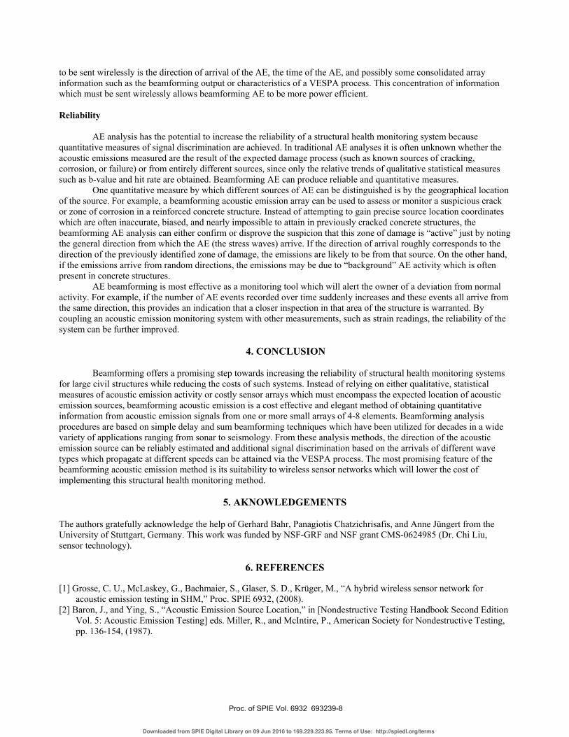
to be sent wirelessly is the direction of arrival of the AE, the time of the AE, and possibly some consolidated array information such as the beamforming output or characteristics of a VESPA process. This concentration of information which must be sent wirelessly allows beamforming AE to be more power efficient. Reliability AE analysis has the potential to increase the reliability of a structural health monitoring system because quantitative measures of signal discrimination are achieved. In traditional AE analyses it is often unknown whether the acoustic emissions measured are the result of the expected damage process (such as known sources of cracking, corrosion, or failure) or from entirely different sources, since only the relative trends of qualitative statistical measures such as b-value and hit rate are obtained. Beamforming AE can produce reliable and quantitative measures. One quantitative measure by which different sources of AE can be distinguished is by the geographical location of the source. For example, a beamforming acoustic emission array can be used to assess or monitor a suspicious crack or zone of corrosion in a reinforced concrete structure. Instead of attempting to gain precise source location coordinates which are often inaccurate, biased, and nearly impossible to attain in previously cracked concrete structures, the beamforming AE analysis can either confirm or disprove the suspicion that this zone of damage is �“active�” just by noting the general direction from which the AE (the stress waves) arrive. If the direction of arrival roughly corresponds to the direction of the previously identified zone of damage, the emissions are likely to be from that source. On the other hand, if the emissions arrive from random directions, the emissions may be due to �“background�” AE activity which is often present in concrete structures.

AE beamforming is most effective as a monitoring tool which will alert the owner of a deviation from normal activity. For example, if the number of AE events recorded over time suddenly increases and these events all arrive from the same direction, this provides an indication that a closer inspection in that area of the structure is warranted. By coupling an acoustic emission monitoring system with other measurements, such as strain readings, the reliability of the system can be further improved.

4. CONCLUSION Beamforming offers a promising step towards increasing the reliability of structural health monitoring systems

for large civil structures while reducing the costs of such systems. Instead of relying on either qualitative, statistical measures of acoustic emission activity or costly sensor arrays which must encompass the expected location of acoustic emission sources, beamforming acoustic emission is a cost effective and elegant method of obtaining quantitative information from acoustic emission signals from one or more small arrays of 4-8 elements. Beamforming analysis procedures are based on simple delay and sum beamforming techniques which have been utilized for decades in a wide variety of applications ranging from sonar to seismology. From these analysis methods, the direction of the acoustic emission source can be reliably estimated and additional signal discrimination based on the arrivals of different wave types which propagate at different speeds can be attained via the VESPA process. The most promising feature of the beamforming acoustic emission method is its suitability to wireless sensor networks which will lower the cost of implementing this structural health monitoring method.

5. AKNOWLEDGEMENTS

The authors gratefully acknowledge the help of Gerhard Bahr, Panagiotis Chatzichrisafis, and Anne Jüngert from the University of Stuttgart, Germany. This work was funded by NSF-GRF and NSF grant CMS-0624985 (Dr. Chi Liu, sensor technology).

6. REFERENCES [1] Grosse, C. U., McLaskey, G., Bachmaier, S., Glaser, S. D., Krüger, M., �“A hybrid wireless sensor network for

acoustic emission testing in SHM,�” Proc. SPIE 6932, (2008). [2] Baron, J., and Ying, S., �“Acoustic Emission Source Location,�” in [Nondestructive Testing Handbook Second Edition

Vol. 5: Acoustic Emission Testing] eds. Miller, R., and McIntire, P., American Society for Nondestructive Testing, pp. 136-154, (1987).



[3] Fowler, T., Yépez, L., Barnes, C., �“Acoustic emission monitoring of reinforced and prestressed concrete structures,�” Proc. SPIE 3400, 281-298, (1998).

[4] Spencer, S. �“The two-dimensional source location problem for time differences of arrival at minimal element monitoring arrays,�” J. Acoust. Soc. Am. 121(6), 3579-3594, (2007)

[5] Ge, M., and Hardy, H.R., �“The Role of Transducer Array Geometry in AE/MS Source Location,�” Fifth Conference on Acoustic Emission/Microseismic Activity in Geologic Structures and Materials, Pennsylvania State University, June 11-13 (1991).

[6] Rost, S., and Thomas, C., �“Array seismology: methods and applications,�” Rev. of Geophys., 40(3), 1-27 (2002). [7] Haykin, S., �“Radar processing for angle of arrival estimation�” in [Array Signal Processing], edited by S. Haykin,

Prentice Hall, New Jersey (1985). [8] Carter, C. �“Time delay estimation for passive sonar signal processing,�” IEEE Trans. Acoust., Speech, Signal

Process., ASSP-29(3), 463-470, (1981). [9] Azar, L., and Wooh, S., �“Experimental characterization of ultrasonic phased arrays for nondestructive evaluation of

concrete structures,�” Materials Evaluation, pp. 135-140 February, (1999). [10] Santoni, G., Yu, L., Xu, B., and Giurgiutiu, V., �“Lamb wave-mode tuning of piezoelectric wafer active sensors for

structural health monitoring,�” J. of Vibration and Acous., Trans. ASME, 129(6), 752-762, (2007). [11] Sundararaman, S, Adams, D, Rigas, E, �“Structural Damage Identification in Homogeneous and Heterogeneous

Structures Using Beamforming,�” Struct. Health Monitoring 4(2), 171-190 (2005). [12] Graff, K, [Wave Motion in Elastic Solids], Oxford University Press, Mineola, NY, Chapters 5 and 6, (1975). [13] Aki, K., Richards, P. G., [Quantitative Seismology: Theory and Methods], Freeman, San Francisco, Chapter 4,

1980. [14] Johnson, D. H., and Dudgeon, D. E. [Array Signal Processing: Concepts and Techniques], PTR Prentice Hall, New

Jersey, (1993). [15] Dudgeon, D. �“Fundamentals of Digital Array Processing,�” Proc. IEEE, 65(6), 898-904 (1977). [16] Van Veen, B., Buckley, K., �“Beamforming: a versatile approach to spatial filtering,�” IEEE ASSP Magazine, 5(2), 4-

24, (1988). [17] Ge, M., and Kaiser, P. K., �“Interpretation of Physical Status of Arrival Picks for Microseismic Source Location,�”

Bull. Seis. Soc. of A., 80, 1643-1660, (1990). [18] Doornbos, D., and Husebye, E., �“Array analysis of PKP phases and their precursors,�” Phys. Earth Planet. Interiors

5, 387-399 (1972). [19] Grosse, C. U., Glaser, S.D. and Krüger, M., �“Condition monitoring of concrete structures using wireless sensor

networks and MEMS,�” Proc. SPIE, 6174, 61741C, (2006). [20] Schechinger, B. (Schallemissionsanalyse als Überwachungsinstrument für Schädigung in Stahlbeton) (Acoustic

emission analysis as a monitoring tool for reinforced concrete deteriorations) Ph.D. dissertation, Eidgenössische Technische Hochschule Zürich (ETH), Zürich, Switzerland, 145 p (2005).



Acoustic emission beamforming for enhanced damage detection · Acoustic emission beamforming for...

Documents

Transcript of Acoustic emission beamforming for enhanced damage detection · Acoustic emission beamforming for...