Acoustic Beamforming using a TDS3230 DSK:Final Report

Steven Bell Nathan WestStudent Member, IEEE Student Member, IEEE

Electrical and Computer EngineeringOklahoma Christian University

i

CONTENTS

I Introduction 1

II Theory 1II-A Delay and Sum Method . . . . . . . . . . . . . . . . . . . . . . . . . . . . . . . . . . . . . . 1II-B Microphone Array Design . . . . . . . . . . . . . . . . . . . . . . . . . . . . . . . . . . . . 1

II-B1 Microphone spacing . . . . . . . . . . . . . . . . . . . . . . . . . . . . . . . . . . 1

III Simulation 2III-A Source localization . . . . . . . . . . . . . . . . . . . . . . . . . . . . . . . . . . . . . . . . 2III-B Spatial Filtering . . . . . . . . . . . . . . . . . . . . . . . . . . . . . . . . . . . . . . . . . . 3

IV System Requirements 3

V Design 4V-A Hardware . . . . . . . . . . . . . . . . . . . . . . . . . . . . . . . . . . . . . . . . . . . . . . 4V-B DSP Software . . . . . . . . . . . . . . . . . . . . . . . . . . . . . . . . . . . . . . . . . . . 4V-C Interface Software . . . . . . . . . . . . . . . . . . . . . . . . . . . . . . . . . . . . . . . . . 5

V-C1 DSK-PC Interface . . . . . . . . . . . . . . . . . . . . . . . . . . . . . . . . . . . 5V-C2 Interface GUI . . . . . . . . . . . . . . . . . . . . . . . . . . . . . . . . . . . . . 5

VI Test Methods 6VI-A Source localization . . . . . . . . . . . . . . . . . . . . . . . . . . . . . . . . . . . . . . . . 6VI-B Spatial filtering . . . . . . . . . . . . . . . . . . . . . . . . . . . . . . . . . . . . . . . . . . 6

VII Results 6

VIII Discussion 6VIII-A Sources of difficulty . . . . . . . . . . . . . . . . . . . . . . . . . . . . . . . . . . . . . . . . 6

IX Conclusion 7

References 7

Appendix A: MATLAB code for beam-sweep source localization 8

Appendix B: MATLAB code for spatial filtering 11

Appendix C: C code for main processing loop 14

Appendix D: C code for summing delays 16

Appendix E: C code for calculating delays 17

Appendix F: Java Code - Main 17

Appendix G: Java Code for Beamformer Communication 18

Appendix H: Java Code for Beam Display 21

1

Abstract—Acoustic beamforming is the use of a micro-phone array to determine the location of an audio sourceor to filter audio based on its direction of arrival. For thisproject, we simulated and implemented a real-time acous-tic beamformer using MATLAB for simulations and theTDS3230 DSK for the real-time implementaion. Althoughthe final system does not meet all of our initial goals, itdoes successfully demonstrate beamforming concepts.

I. INTRODUCTION

Most broadly, beamforming is the use of an arrayof antennas - or in the case of audio, microphones- to perform signal processing based on the spatialcharacteristics of a signal. We will discuss two primaryforms of beamforming in this document: source localiza-tion and spatial filtering. Source localization attempts todetermine the location in space a signal originated from,while spatial filtering creates an electronically-steerablenarrow-beam antenna, which has gain in one directionand strong attenuation in others. Spatial filtering systemsand corresponding transmission techniques can replacephysically moving antennas, such as those used for radar.

Acoustic source localization is familiar to all of us:we have two ears, and by using them together, our braincan tell where sounds come from. Similarly, our brainsare able to focus on one particular sound and tune outthe rest, even when the surrounding noise is much louderthan the sound we are trying to hear.

II. THEORY

A. Delay and Sum Method

If we have an array of microphones and sufficientsignal-processing capability, we can measure the timedelay from the time the sound strikes the first micro-phone until it strikes the second. If we assume wavesoriginate far enough away that we can treat the edge ofits propagation as a plane, then the delays are simple tomodel with trigonometry as shown in Figure 1.

Suppose we have a linear array of microphones, m1

through mn, each spaced Dmic meters apart. ThenDdelay, the extra distance the sound has to travel foreach successive microphone, is given by

Ddelay = Dmic · cos (θ) (1)

At sea level, the speed of sound is 340.29 ms , which

means that the time delay is

Tdelay =Dmic

340.29 ms

· cos (θ) (2)

By reversing this delay for each microphone and sum-ming the inputs, we can recover the original signal. If asignal comes from a different direction, the delays willbe different, and as a result, the individual signals willnot line up and will tend to cancel each other when

Figure 1. Planar wavefront approaching a linear microphone array.

added. This essentially creates a spatial filter, which wecan point in any direction by changing the delays.

To determine the direction a signal came from, we cansweep our beam around the room, and record the totalpower of the signal recieved for each beam. The sourcecame from the direction with the highest-power signal.

B. Microphone Array Design

Microphone arrays can be nearly any shape: linear, cir-cular, rectangular, or even spherical. A one-dimensionalarray allows beamforming in one dimension; additionalarray dimensions allow for 2-dimensional beamforming.Given the limited number of microphones and amountof time we have, a linear array is the best choice.

1) Microphone spacing: The spacing of the micro-phones is driven by the intended operating frequencyrange.

For spatial filtering, a narrower beam width is anadvantage, because signals which are not directly fromthe intended direction are attenuated. A narrow beamwidth is analogous to a narrow transistion band fora tranditional filter. Lower frequencies will correlatebetter with delayed versions of themselves than highfrequencies, so the lower the frequency, the broader thebeam. Conversely, a longer array will result in a greaterdelay between the end microphones, and will thus reducethe beam width.

At the same time, the spacing between microphonesdetermines the highest operating frequency. If the wave-length of the incoming signal is less than the spacingbetween the microphones, then spatial aliasing occurs.An example is shown in Figure 2.

The spacing between microphones causes a maximumtime delay which, together with the sampling frequency,limits the number of unique beams that can be made.

2

2

4

6

30

210

60

240

90

270

120

300

150

330

180 0

Figure 2. Spatial aliasing. The source is 1 kHz, located at 135 degrees.An image appears at approximately 50 degrees, which means thatsound coming from that direction is indistinguishable from the desiredsource.

The maximum number of beams, maxbeams, is shownmathematically in Equation 3.

maxbeams = 2 · Fs · timespacing (3)

The variable timespacing is the maximum amount oftime it takes for sound to travel from one microphone toan adjacent microphone, as the case when the source isalong the line created by the array.

III. SIMULATION

Source localization and spatial filtering both use es-sentially the same simulation code. First, we define acoordinate system where our microphones are placed,with the origin at the center of our linear array. Wedefined the distance between microphones to be 25cm, making total array lengths of 75 cm for a fourmicrophone array and 25 cm for a two microphone array.

A. Source localization

In the source localization code, a single source islocated 10 meters away from the center of the array.A loop creates thirty beams which cover a 180-degreerange, and the power for each beam is computed. Figure3 shows the power sweeps for five different sourceangles. Note that in each case, the maximum power isexactly at the angle the sound originates from.

Using the beam-sweeping technique, we examined therelative effects of the number of microphones and thesource frequency. Figure 4 shows a comparison of thebeamwidth as a function of the number of microphones.Figure 5 shows a comparison of beam width versus fre-quency. Note that higher frequencies produce narrowerbeams, so long as spatial aliasing does not occur.

30

210

60

240

90

270

120

300

150

330

180 0

Figure 3. Source localization simulation using a 400 Hz source anda 4-microphone array. The source was located at 0, 45, 90, 135, and180 degrees.

30

210

60

240

90

270

120

300

150

330

180 0

Two

Four

Six

Figure 4. Comparison of beam width versus the number of micro-phones. The source was 400 Hz at 90 degrees.

30

210

60

240

90

270

120

300

150

330

180 0

Figure 5. Comparison of beam width versus frequency using 2microphones. The frequencies range from 200 Hz to 700 Hz inincrements of 100 Hz. Higher frequencies produce narrower beams.

3

20

40

60

80

100

30

210

60

240

90

270

120

300

150

330

180 0

Figure 6. Decibel-scale plot of a 4-microphone array beampattern fora 600 Hz signal at 90 degrees. Note the relatively large sidelobes onboth sides of the main beam.

Figure 6 shows a plot of the beam in decibels, whichbrings out a pair of relatively large sidelobes. Thesecan be reduced by windowing the microphone inputs, inthe same way that a filter can be windowed to producelower sidelobes in exchange for a wider transition band.However, this windowing is unlikely to be useful for oursmall array.

The MATLAB source code is in Appendix A.

B. Spatial Filtering

For spatial filtering, one source is placed at 10 mnormal to the array and 10 m tangentially from the centerof the array. Using this location as a reference, we canplace a secondary source equidistant from the center ofthe microphone array but some degree offset.

For this simulation set we used two offsets, 60 degreesand 90 degrees. The formed beam was looking 45degrees away from the array (towards the source at 10,10). Two microphones were used in simulations becauseof suggestions by Dr. Waldo and four were used becausethat is the maximum number of input channels on ourhardware. In Figure 7 the simulation has a variablenumber of microphones with the sources separated by60 and 90 degrees. This simulation was the influence forthe specification calling for 3dB down on a 60 degreesource separation. The SNR is improved drastically whenthe same sources are separated by 90 degrees still usinga 2 microphone array, as seen in Figure 8.

Figures 9 and 10 show similar but improved resultswhen the array is increased to four microphones.

The MATLAB source code is in Appendix B.

IV. SYSTEM REQUIREMENTS

• The system must have at least two microphones asits input.

0 100 200 300 400 500 600 700−60

−50

−40

−30

−20

−10

0FFT of the received signal

Rela

tive m

agnitude o

f sig

nal (d

B)

Frequency (Hz)

Figure 7. The noise source at 300Hz is attenuated by about 3dB usingan array of two microphones with sources separated by 60 degrees.

0 100 200 300 400 500 600 700−50

−45

−40

−35

−30

−25

−20

−15

−10

−5

0FFT of the received signal

Rela

tive m

agnitude o

f sig

nal (d

B)

Frequency (Hz)

Figure 8. An array of two microphones with sources separated by 90degrees will attenuate the noise source by about 13dB.

0 100 200 300 400 500 600 700−60

−50

−40

−30

−20

−10

0FFT of the received signal

Rela

tive m

agnitude o

f sig

nal (d

B)

Frequency (Hz)

Figure 9. An array of four microphones with sources separated by60 degrees results in the noise source attenuated by about 12dB.

4

0 100 200 300 400 500 600 700−50

−45

−40

−35

−30

−25

−20

−15

−10

−5

0FFT of the received signal

Rela

tive m

agnitude o

f sig

nal (d

B)

Frequency (Hz)

Figure 10. With an array of four microphones with sources separatedby 90 degrees the noise signal is about 12dB down from the signal weattempted to isolate.

• The system must have a GUI running on a computerwhich communicates with the DSK board.

• In localization mode:– The system will be able to locate the direction

of a 400 Hz tone between -90 and +90 degrees,with +/- 5 degrees error. This target tone willbe significantly above the noise threshold in theroom.

– The GUI must display the direction of theincoming sound with a latency less than 1second.

• In directional enhancement mode:– The GUI must allow the user to select a partic-

ular direction to listen from, between -90 and+90 degrees, and with a resolution of at least10 degrees.

– The system should play the selected directionaloutput via one of the line out channels.

– A 300 Hz noise source with the same powerwill be placed 60 degrees apart from thedesired signal source. The directional outputshould give a signal-to-noise ratio of at least3 dB.

• The system will operate properly when the soundsources are at least 4 meters away from the micro-phone array.

V. DESIGN

The acoustic beam forming system consists of threehigh level subsystems: the microphone array, the DSKboard, and a GUI running on a PC. A block diagramshowing the interconnections of these subsystems isshown in Figure 11. The microphone array should con-tain two to four microphones placed in a straight line 25

Figure 11. Functional block diagram.

Figure 12. Flowchart for the main DSP software.

cm apart. Theses microphones will be connected to themicrophone inputs on the DSK_AUDIO4 daughtercard.The DSK will be programmed to process a 256 sampleblock at a time. The software delays each microphone’sinput by a different number of samples then adds eachinput to create the output. In source localization mode,the power of the output is calculated and sent to the PCGUI. In spatial filtering mode, the output is passed toone of the board’s output channels.

A. Hardware

In addition to the standard DSK board provided tothe DSP class we will be using the Educational DSPDSK_AUDIO4 daughtercard, which has four input chan-nels. Each of these channels will be connected to one ofthe generic mono microphones provided to the class byDr. Waldo. The placement of the microphones introducesa physical variable to the system that is important to theoperation of hardware: according to our specificationsand simulations the microphones should be spaced 25cm apart. Ideally, they will face the direction of incomingacoustic sources for maximum input power.

B. DSP Software

The foundation of our DSP software is the samplecode provided by Educational DSP and modified by Dr.Waldo. This code initializes the DSP and the codec andcalls a processing function that provides samples fromall four input channels. Using this as a base we willimplement our main function inside of the processingfunction provided. In this main file we will also includea file that defines our sum and delay functions whichwill exist in their own files.

The main software branch opens a RTDX channel withthe PC GUI and keeps track of the current operatingmode. The mode is a boolean value where a TRUEmeans spatial filtering mode and a FALSE means sourcelocalization mode. In the spatial aliasing mode we doa simple delay and sum of the input data. The delay isgiven by the GUI. In localization mode the current outputis also the delay and sum of the input; however, the delaysweeps from a minimum possible delay to a maximumpossible delay defined by the number of samples it takesto go from −90o to 90o. After every delay and sumoperation the delay/power pairs will be sent to the GUIfor display via the RTDX channel. The flow of this isshown in Figure 12.

5

Figure 13. Flowchart for the function that calculates the number ofsamples to delay each microphone’s input by.

Figure 14. Flowchart for the DSK function that calculates the currentoutput sample.

To determine how much to delay each microphone bywe get the number of samples each microphone shouldbe delayed by from the GUI and multiply by the orderof that microphone in the array. The first microphone inthe array is defined as microphone 0 and has a 0 delay.If the delay we get from the GUI is negative the order isreversed so that the earliest input always has a 0 delay.The calcDelay function will return a pointed to an arraycalled delays. Figure 13 shows the structure and flow forcalcDelay.

The sum function accepts the current four input sam-ples and delay from the GUI and passes it to calcDelays.Figure 14 shows a program flow for this function. Itwill have a reverse index tracked buffer so that ifi=5 is the current input i=6 is the oldest input andi=4 is the second most recent input. This requiresfewer rollover-error-checking comparisons relative to aforward-tracking buffer, which should give us an incre-mental speed improvement.

C. Interface Software

1) DSK-PC Interface: The PC will communicate withthe DSK board using RTDX 2.0. For speed, the DSKwill only perform integer operations; thus, the PC willperform the floating-point work of translating delaysto angles and vice-versa. There will be two RTDX IOchannels, one going each direction.

a) Power-vs-Delay to PC:• Delay will be a 2’s complement 8 bit signed num-

ber, which represents the relative delay betweenmicrophones. This will be calculated from the mi-crophone spacing and the speed of sound.

• Power will be a 16-bit unsigned number, whichholds the relative power of the signal for a particularbeam.

In order for these two values to remain correlated, wewill interleave both on one channel, and signal the startof each new delay-power pair using the value 0xFF. Thiswill allow our system to recover from lost or delayedbytes.

This data will only be sent when the system is insource localization mode.

Figure 15. Byte transmission order for DSK→ PC communication

Table IBYTE SIGNALS FOR PC→DSK COMMUNICATION

Use Code RangeMicrophone time spacing 0-100Number of microphones 2-4

Mode 1,2Beam selection -100 to +100

Figure 16. Byte transmission order for PC → DSK communication

We found that we did not need any synchronizationbytes, and we trimmed the communictation down to asingle byte for the power paired with a single byte fordelay. This was intended to speed up RTDX communi-cation, but was not successful.

b) Settings to DSK Board: The GUI will controlseveral settings, summarized in Table I Physical variablessuch as microphone spacing and number of microphonesneed to be easily changed by software in real time, andthe GUI provides an interface for users to the DSK tochange the operation as required.

The byte stream will follow the same format as theDSK to PC stream. Data will be sent in 3 byte packetsas shown in Figure 16. Packets will only be sent whenthere is new data, so we expect the number of packetsper second to be very low.

We did not implement this due to time constraints.2) Interface GUI: The interface software will be

written in Java. An overview of the main classes is shownin Figure 17.

The Beamformer class handles the low-level transla-tion and communication with the DSK board. It convertsfrom sample delays to angles and vice-versa, convertsbooleans to code values, and floating-point values tointegers for high-speed communication.

The BeamDisplay is a GUI class which displays thebeam power levels and sound direction on a polar plot,similar to the simulation plots. It will use the JavaAWT/Swing toolkit and associated drawing classes toimplement a custom drawable canvas. Clicking on thedisplay will select the direction to use when in spatialfiltering mode.

The Settings panel will contain a series of standardSwing components to select the operating mode, numberof microphones, microphone spacing, the number ofbeams per sweep. It will have a pointer to the Beam-former object, so it can configure it directly.

The MainWindow class creates the main GUI window,the display and control panels, and the connection tothe DSK board. Once running, it will regularly pollthe beamformer class for new data, and update the

6

MainWindow

+guiComponents

-connectToDSK()

-initializeGui()

-disconnect()

ControlPanel

+modeSelect

+numBeams

+numMicrophones

+microphoneSpacing

-initialize()

BeamDisplay

+canvas: JPanel

-initialize()

+update(newData)

Beamformer

-ControlChannel: RTDX Channel

-DataChannel: RTDX Channel

+setMode(mode:int)

+setNumBeams(newNum:int)

+setNumMicrophones(newNum:int)

+setMicrophoneSpacing(newSpacing:double)

+setFilterAngle(newAngle:int)

+update()

+hasNewData()

+getBeamPower()

Figure 17. Class Diagram for the GUI

BeamDisplay accordingly.

VI. TEST METHODS

A. Source localization

To test performance of the source localization methodwe set up two microphones 25cm apart. Using a meterstick to keep a contsant radius, an amplified speaker wasswept radially across the plane level with the micro-phones. A digital oscilloscope was used to measure theRMS voltage of the processed output. We also observedthe beam displayed on the GUI.

B. Spatial filtering

Because of time constraints and unexpected difficul-ties with other parts of the project, we did not explicitlytest spatial filtering.

To test the spatial filtering mode, we would have setup two sources at for different frequencies equidistantfrom the array with a 90 degree arc length seperation.The DSK would process the data with a beam formedtowards one of the sources and feed the output was toa digital oscilloscope or MATLAB/Simulink GUI set toview the FFT. Using this method, we could compare therelative strengths of the signals.

VII. RESULTS

Our system is able to do beamforming with 2 mi-crophones, and display the result on a PC GUI. Byobservation, the beamwidth is about what we expectedfor a 2-microphone array.

We were unable to get any kind of beamformingto work with four microphones. After getting the 2-microphone system working, we switched to 4 by chang-ing a #define in our code and connecting two addi-tional microphones to the DSK expansion board. Whenwe ran the GUI, we were unable to observe any kind oflocalization.

Each adjacent pair of microphones worked in a 2-microphone beamformer, so we believe that it was nota simple case of one microphone not working properlyor a result of mixing up the order of the microphones.We performed a test where we merely averaged theinputs from the four microphones and sent that valueto the output, which is equivalent to forming a beamperpendicular to the array. Using one of the speakersas an audio source and measuring the RMS voltage ofthe output on the oscilloscope, we manually checked thedirectionality of the array. We were unable to measureany significant difference between the sound source be-ing directly orthogonal to the array and at a small angleto it. This indicates that at least part of the problem isnot due to our software. There may have been additionalproblems with our software for four microphones, butbecause we were unable to get this simple test working,we did not test our software further.

VIII. DISCUSSION

A. Sources of difficulty

We identified several factors which contributed to oursystem’s failure to meet its requirements.

First, there were several acoustic problems. We foundthat the supplied microphones are very directional -they are specifically labeled “unidirectional”. Becausethe beamforming system assumes omnidirectional input,unidirectional microphones will cause oblique signals tobe attenuated. This is fine when the desired beam is per-pendicular to the array, but is suddenly a problem whenthe goal is to amplify oblique signals over orthogonalones.

The audio input level from the microphones seemedto be rather low, producing averaged output values inthe single-millivolt range. We are not sure if there is away to configure additional gain on the DSK board, orif using different microphones would help. Due to thelow input level, we had to play the signal very loudly onthe speakers and keep them within one or two meters ofthe array.

A 1-meter source distance clearly violates the farfieldplane-wave assumption - our initial specification as-sumed that 4 meters was farfield. This may have causedsome problems, but re-running our MATLAB simulationusing a source only 1m away produced a beam virtuallyindistinguishable from a 10-meter beam.

7

We also experienced very strong echoes in the room,because of its cement construction and solid woodlab benches. Working in an environment with reducedechoes would probably have yielded better results. Thiswas evident during late nights in the lab when peopleworking in the ASAP room and janitorial staff wouldpeek into the room to find the very loud noise echoingthroughout the HSH.

On the software side, we experienced difficulties get-ting the bandwidth we desired over RTDX. I had alsoseen poor RTDX performance before, when sending datafrom a PC to the DSK during the cosine generation lab.There are several possible causes of this: One is thatwe only send a few bytes at a time, but do it dozensof times per second. Recommendations we found onlinesuggested that filling the RTDX queue and sending largepackets of data is the fastest way to send data.

Another likely cause is our DSK boards. We read amailing list correspondence between someone who isfamiliar with this family of DSKs and a hapless hobbyisthaving similar issues. The “expert” claimed that thereis obfuscation hardware on the DSK boards introducedby Spectrum Digital that slows down RTDX communi-cation. It was mentioned that a possible workaround isusing the JTAG connector on the DSK board, but thehardware required for this is not readily available (andthe JTAG port is blocked by the DSP_AUDIO_4). Welooked at high-speed RTDX, but it is not supported onthis platform.

IX. CONCLUSION

Although we did not meet our initial specifications,our project was still somewhat successful. We were ableto implement a working beamforming system, and mostof the problems we encountered were limitations of ourequiment which were not under our control.

REFERENCES

[1] M. Brandstein and D. Ward, eds., Microphone Arrays: Signal Pro-cessing Techniques and Applications. Berlin, Germany: Springer,2001.

[2] J. Benesty, J. Chen, and Y. Huang, Microphone Array SignalProcessing. Berlin, Germany: Springer, 2008.

[3] J. Chen, L. Yip, J. Elson, H. Wang, D. Maniezzo, R. Hudson,K. Yao, and D. Estrin, “Coherent Acoustic Array Processing andLocalization on Wireless Sensor Networks,” Proceedings of theIEEE, vol. 91, no. 8, pp. 1154–1162, 2003.

[4] J. C. Chen, K. Yao, and R. E. Hudson, “Acoustic Source Localiza-tion and Beamforming: Theory and Practice,” EURASIP Journalon Applied Signal Processing, pp. 359–370, 2003.

[5] T. Haynes, “A primer on digital beamforming,” Spectrum SignalProcessing, 1998.

[6] W. Herbordt and W. Kellermann, “Adaptive Beamforming for Au-dio Signal Acquisition,” Adaptive Signal Processing: Applicationsto Real-World Problems, pp. 155–196, 2003.

[7] R. A. Kennedy, T. D. Abhayapala, and D. B. Ward, “Broadbandnearfield beamforming using a radial beampattern transformation,”IEEE Transactions on Signal Processing, vol. 46, no. 8, pp. 2147–2156, 1998.

[8] R. J. Lustberg, “Acoustic Beamforming Using Microphone Ar-rays,” Master’s thesis, Massachusetts Institute of Technology,Cambridge, MA, June 1993.

[9] N. Mitianoudis and M. E. Davies, “Using Beamforming in theAudio Source Separation Problem,” in 7th Int Symp on SignalProcessing and its Applications, no. 2, 2003.

8

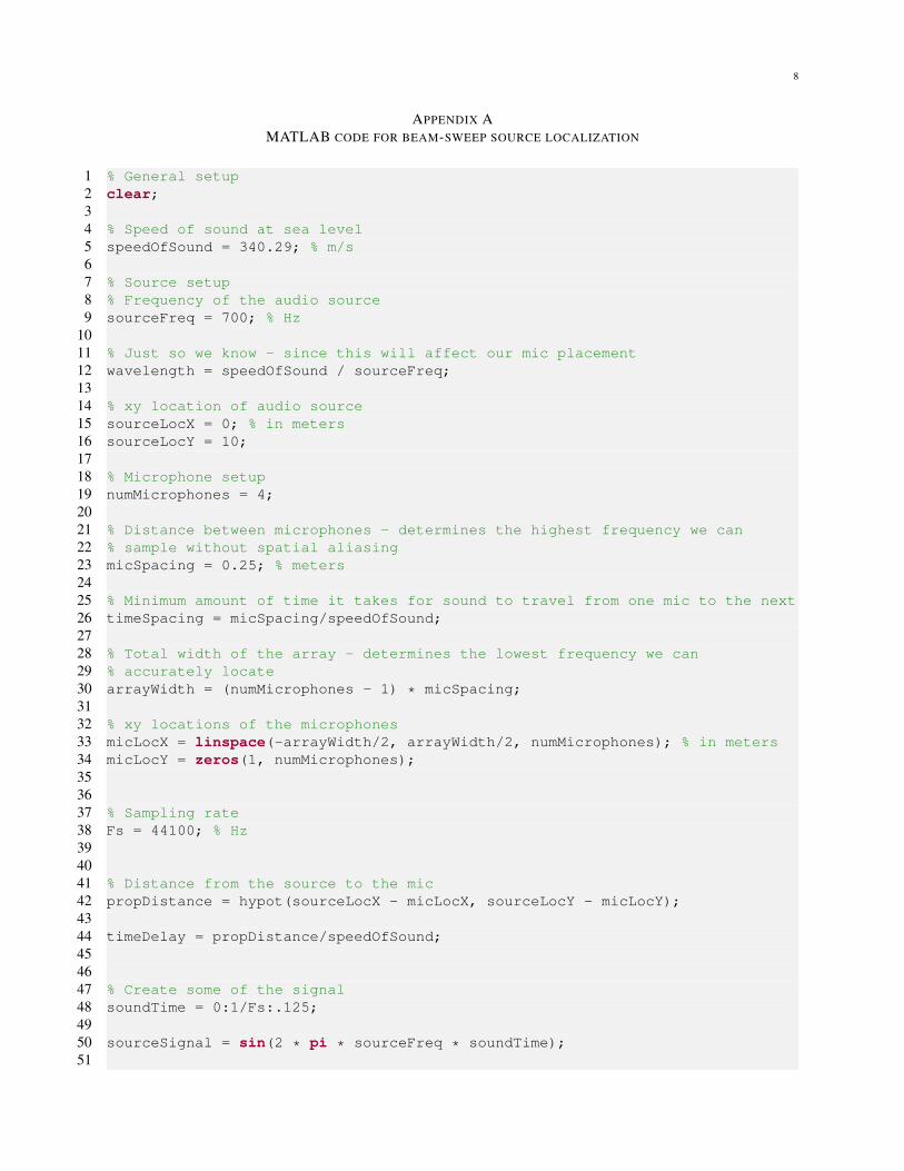
APPENDIX AMATLAB CODE FOR BEAM-SWEEP SOURCE LOCALIZATION

1 % General setup2 clear;34 % Speed of sound at sea level5 speedOfSound = 340.29; % m/s67 % Source setup8 % Frequency of the audio source9 sourceFreq = 700; % Hz

1011 % Just so we know - since this will affect our mic placement12 wavelength = speedOfSound / sourceFreq;1314 % xy location of audio source15 sourceLocX = 0; % in meters16 sourceLocY = 10;1718 % Microphone setup19 numMicrophones = 4;2021 % Distance between microphones - determines the highest frequency we can22 % sample without spatial aliasing23 micSpacing = 0.25; % meters2425 % Minimum amount of time it takes for sound to travel from one mic to the next26 timeSpacing = micSpacing/speedOfSound;2728 % Total width of the array - determines the lowest frequency we can29 % accurately locate30 arrayWidth = (numMicrophones - 1) * micSpacing;3132 % xy locations of the microphones33 micLocX = linspace(-arrayWidth/2, arrayWidth/2, numMicrophones); % in meters34 micLocY = zeros(1, numMicrophones);353637 % Sampling rate38 Fs = 44100; % Hz394041 % Distance from the source to the mic42 propDistance = hypot(sourceLocX - micLocX, sourceLocY - micLocY);4344 timeDelay = propDistance/speedOfSound;454647 % Create some of the signal48 soundTime = 0:1/Fs:.125;4950 sourceSignal = sin(2 * pi * sourceFreq * soundTime);51

9

52 % Delay it by the propagation delay for each mic53 for ii = 1:numMicrophones54 received(ii,:) = delay(sourceSignal, timeDelay(ii), Fs);55 end5657 % Plot the signals received by each microphone58 % plot(received’);5960 % Now it’s time for some beamforming!61 % Create an array of delays62 numBeams = 60;63 beamDelays = linspace(-timeSpacing, timeSpacing, numBeams);6465 for ii = 1:numBeams66 summedInput = zeros(1, length(sourceSignal));67 for jj = 1:numMicrophones68 if(beamDelays(ii) >= 0)69 % Delay the microphones by increased amounts as we go left to right70 summedInput = summedInput + ...71 delay(received(jj,:), beamDelays(ii) * (jj - 1), Fs);72 else73 % If the beam delay is negative, that means we want to increase the74 % delay as we go right to left.75 summedInput = summedInput + ...76 delay(received(jj,:), -beamDelays(ii) * (numMicrophones - jj), Fs);77 end78 end79 % Calculate the power of this summed beam80 power(ii) = sum(summedInput .^ 2);81 end8283 % directions = linspace(pi, 0, numBeams);84 directions = acos(linspace(-1, 1, numBeams));8586 polar(directions, power/max(power), ’-b’);

10

1 function [outputSignal] = delay(inputSignal, time, Fs)2 % DELAY - Simulates a delay in a discrete time signal3 %4 % USAGE:5 % outputSignal = delay(inputSignal, time, Fs)6 %7 % INPUT:8 % inputSignal - DT signal to operate on9 % time - Time delay to use

10 % Fs - Sample rate1112 if(time < 0)13 error(’Time delay must be positive’);14 end1516 outputSignal = [zeros(1, floor(time * Fs)), inputSignal];1718 % Crop the output signal to the length of the input signal19 outputSignal = outputSignal(1:length(inputSignal));

11

APPENDIX BMATLAB CODE FOR SPATIAL FILTERING

123 % General setup4 clear;56 % The frequencies we are interested in are:7 % Right now this is optimized for sources between 100 and 500 Hz8 % Change this to whatever range you are interested in.9 fmin = 00; % Hz

10 fmax = 700;% Hz1112 % Speed of sound at sea level13 speedOfSound = 340.29; % m/s1415 % Source setup16 % Frequency of the audio sources17 source1Freq = 300; % Hz18 source2Freq = 400; % Hz1920 % Just so we know - since this will affect our mic placement21 wavelength1 = speedOfSound / source1Freq;22 wavelength2 = speedOfSound / source2Freq;2324 degreesApart=60;25 % xy location of audio source26 source1LocX = sqrt(10^2 + 10^2)*cosd(45+degreesApart); % in meters27 source1LocY = sqrt((10^2 + 10^2)-source1LocX^2);28 source2LocX = 10; % Secondary source29 source2LocY = 10;3031 % Microphone setup32 numMicrophones = 2;3334 % Distance between microphones - determines the highest frequency we can35 % sample without spatial aliasing36 micSpacing = 0.25; % meters3738 % Minimum amount of time it takes for sound to travel from one mic to the next39 timeSpacing = micSpacing/speedOfSound;4041 % Total width of the array - determines the lowest frequency we can42 % accurately locate43 arrayWidth = (numMicrophones - 1) * micSpacing;4445 % xy locations of the microphones46 micLocX = linspace(-arrayWidth/2, arrayWidth/2, numMicrophones); % in meters47 micLocY = zeros(1, numMicrophones);484950 % Sampling rate51 Fs = 96000; % Hz

12

525354 % Distance from the source to the mic55 prop1Distance = hypot(source1LocX - micLocX, source1LocY - micLocY);56 prop2Distance = hypot(source2LocX - micLocX, source2LocY - micLocY);5758 time1Delay = prop1Distance/speedOfSound;59 time2Delay = prop2Distance/speedOfSound;6061 % Create some of the signal62 soundTime = 0:1/Fs:.125;6364 source1Signal = sin(2 * pi * source1Freq * soundTime);65 source2Signal = sin(2 * pi * source2Freq * soundTime);6667 % Delay it by the propagation delay for each mic68 for ii = 1:numMicrophones69 received(ii,:) = delay(source1Signal, time1Delay(ii), Fs)...70 + delay(source2Signal, time2Delay(ii), Fs);71 end727374 % Direct the beam towards a location of interest75 angleWanted = 45; % Degrees (for simplicity)76 angleToDelay = angleWanted * pi/180; % Convert to radian7778 % We want to take the fft of the signal only after everymicrophone is79 % getting all of the data from all sources80 deadAirTime = (max([time1Delay, time2Delay]));81 deadAirSamples = deadAirTime * Fs;82 endOfCapture = length(received(1,:));8384 % Start off with an empty matrix85 formedBeam = zeros(1, max(length(received)));8687 % For each microphone add together the sound received88 for jj = 1:numMicrophones89 formedBeam = formedBeam + ...90 delay(received(jj,:), + timeSpacing*sin(angleToDelay) * (jj-1), Fs);91 end9293 % Get the PSD object using a modified covariance94 beamPSD = psd(spectrum.mcov, formedBeam,’Fs’,44100);95 % Get the magnitude of the PSD96 formedSpectrum = abs(fft(formedBeam));97 % The fft sample # needs to be scaled to get frequency98 fftScaleFactor = Fs/numel(formedSpectrum);99

100 % The frequencies we are interested in are:101 % Right now this is optimized for sources between 100 and 500 Hz102 %fmin = 0; % Hz103 %fmax = 600;% Hz104105 % Plot the PSD of the received signal

13

106 figure(1);107 % Get the frequencies and data out of the PSD object108 beamPSDfreqs=beamPSD.Frequencies;109 beamPSDdata = beamPSD.Data;110 % Get the indeces that correspond to frequencies specified above111 indexesToPlot=find(beamPSDfreqs>fmin-1):find(beamPSDfreqs>fmax,1);112 % Actually plot it (in a log10 scale so we have dB)113 plot(beamPSDfreqs(indexesToPlot),20*log10(beamPSDdata(indexesToPlot)));114 title(’PSD using a modified covariance of the received signal’);115 ylabel(’Power/Frequency (dB)’);116 xlabel(’Frequency (Hz)’);117118 % Plot the fft of our received signals119 figure(2);120 maxLimit=round(fmax/fftScaleFactor);121 minLimit=round(fmin/fftScaleFactor);122 if minLimit <= 0123 minLimit = 1;124 end125 f=linspace(0,44100,44100/fftScaleFactor);126127 % This gets all of the fft frequencies we want to look at128 fOfInterest = f(minLimit:maxLimit);129 % Grab the portion of the fft we want to look at130 spectrumOfInterest = formedSpectrum(minLimit:maxLimit);131 % Normalize this so that the max amplitude is at 0db.132 spectrumOfInterest = spectrumOfInterest/max(formedSpectrum);133 % Plot it134 plot(fOfInterest,20*log10(spectrumOfInterest));135 title(’FFT of the received signal’);136 ylabel(’Relative magnitude of signal (dB)’);137 xlabel(’Frequency (Hz)’);

14

APPENDIX CC CODE FOR MAIN PROCESSING LOOP

12 void processing(){3 Int16 twoMicSamples[2];45 Int32 totalPower; // Total power for the data block, sent to the PC6 Int16 tempPower; // Value used to hold the value to be squared and added7 Int16 printCount; // Used to keep track of the number of loops since we last sent data8 unsigned char powerToSend;9

10 Int8 firstLocalizationLoop; // Whether this is our first loop in localization mode11 Int8 delay; // Delay amount for localization mode1213 QUE_McBSP_Msg tx_msg,rx_msg;14 int i = 0; // Used to iterate through samples1516 RTDX_enableOutput( &dataChan );1718 while(1){1920 SEM_pend(&SEM_McBSP_RX,SYS_FOREVER);2122 // Get the input data array and output array23 tx_msg = QUE_get(&QUE_McBSP_Free);24 rx_msg = QUE_get(&QUE_McBSP_RX);2526 // Spatial filter mode2728 // Localization mode29 if(firstLocalizationLoop){30 delay = DELAYMIN;31 firstLocalizationLoop = FALSE;32 }33 else{34 delay++;35 if(delay > DELAYMAX){36 delay = DELAYMIN;37 }38 }3940 // Process the data here41 /* MIC1R data[0]42 * MIC1L data[1]43 * MIC0R data[2]44 * MIC0L data[3]45 *46 * OUT1 Right - data[0]47 * OUT1 Left - data[1]48 * OUT0 Right - data[2]49 * OUT0 Left - data[3]50 */51

15

52 totalPower = 0;5354 for(i=0; i<QUE_McBSP_LEN; i++){5556 // Put the array elements in order57 twoMicSamples[0] = *(rx_msg->data + i*4 + 2);58 twoMicSamples[1] = *(rx_msg->data + i*4 + 3);5960 tx_msg->data[i*4] = 0;61 tx_msg->data[i*4 + 1] = 0;62 tx_msg->data[i*4 + 2] = sum(twoMicSamples, delay);63 tx_msg->data[i*4 + 3] = 0;

16

APPENDIX DC CODE FOR SUMMING DELAYS

Listing 1. sum.h1 #ifndef _SUM_H_BFORM_2 #define _SUM_H_BFORM_3 extern Int16 sum(Int16* newSamples, int delay);4 #endif

Listing 2. sum.c12 #include <std.h>34 #include "definitions.h"5 #include "calcDelay.h"67 /* newSamples is an array with each of the four samples.8 * delayIncrement is the amount to delay each microphone by, in samples.9 * This function returns a "beamed" sample. */

10 Int16 sum(Int16* newSamples, int delayIncrement){11 static int currInput = 0; // Buffer index of current input12 int delays[NUMMICS]; // Amount to delay each microphone by13 int mic = 0; // Used as we iterate through the mics14 int rolloverIndex;15 Int16 output = 0;16 static Int16 sampleBuffer[NUMMICS][MAXSAMPLEDIFF];1718 // Calculate samples to delay for each mic19 // TODO: Only do this once20 calcDelay(delayIncrement, delays);2122 // We used to count backwards - was there a good reason?23 currInput++; // Move one space forward in the buffer2425 // Don’t run off the end of the array26 if(currInput >= MAXSAMPLEDIFF){27 currInput = 0;28 }2930 // Store new samples into sampleBuffer31 for(mic=0; mic < NUMMICS; mic++){32 // Divide by the number of microphones so it doesn’t overflow33 // when we add them34 sampleBuffer[mic][currInput] = newSamples[mic]/NUMMICS;35 }3637 // For each mic add the delayed input to the current output38 for(mic=0; mic < NUMMICS; mic++){39 if(currInput - delays[mic] >= 0){// Index properly?40 output += sampleBuffer[mic][currInput - delays[mic]];41 }42 else{43 // The delay index is below 0, so add the length of the array44 // to keep it in bounds

17

45 rolloverIndex = MAXSAMPLEDIFF + (currInput - delays[mic]);46 output += sampleBuffer[mic][rolloverIndex];47 }48 }4950 return output;5152 }

APPENDIX EC CODE FOR CALCULATING DELAYS

Listing 3. calcDelay.h1 #ifndef _CALC_DELAY_H_2 #define _CALC_DELAY_H_3 extern void calcDelay(int delayInSamples, int* delays);4 #endif

Listing 4. calcDelay.c1 /* calcDelay2 * Accepts delays in samples as an integer3 * and returns a pointer to an array of delays4 * for each microphone.5 *6 * Date: 9 March 20107 */89 #include "definitions.h"

1011 void calcDelay(int delayInSamples, int* delays){12 int mic = 0;13 if(delayInSamples > 0){14 for(mic=0; mic < NUMMICS; mic++){15 delays[mic] = delayInSamples*mic;16 }17 }18 else{19 for(mic=0; mic < NUMMICS; mic++){20 delays[mic] = delayInSamples*(mic-(NUMMICS-1));21 }22 }23 }

APPENDIX FJAVA CODE - MAIN

Listing 5. MainWindow.java1 /* MainWindow.java - Java class which constructs the main GUI window2 * for the project, and sets up communication with the DSK. It also3 * contains the main() method.4 *5 * Author: Steven Bell and Nathan West6 * Date: 9 March 20107 * $LastChangedBy$8 * $LastChangedDate$

18

9 */1011 package beamformer;1213 import java.awt.*; // GUI Libraries1415 import javax.swing.*;1617 public class MainWindow18 {19 JFrame window;20 DisplayPanel display;21 ControlPanel controls;22 static Beamformer beamer;2324 MainWindow()25 {26 beamer = new Beamformer();2728 window = new JFrame("Acoustic Beamforming GUI");29 window.setDefaultCloseOperation(WindowConstants.EXIT_ON_CLOSE);30 window.getContentPane().setLayout(new BoxLayout(window.getContentPane(), BoxLayout.LINE_AXIS));3132 display = new DisplayPanel();33 display.setPreferredSize(new Dimension(500,500));34 display.setAlignmentY(Component.TOP_ALIGNMENT);35 window.add(display);3637 controls = new ControlPanel();38 controls.setAlignmentY(Component.TOP_ALIGNMENT);39 window.add(controls);4041 window.pack();42 window.setVisible(true);4344 beamer.start();45 }4647 public static void main(String[] args)48 {49 MainWindow w = new MainWindow();50 while(true){51 beamer.update();52 w.display.updatePower(beamer.getPower());53 }54 }55 }

APPENDIX GJAVA CODE FOR BEAMFORMER COMMUNICATION

Listing 6. Beamformer.java1 /* Beamformer.java - Java class which interacts with the DSK board2 * using RTDX.3 *

19

4 * Author: Steven Bell and Nathan West5 * Date: 11 April 20106 * $LastChangedBy$7 * $LastChangedDate$8 */9

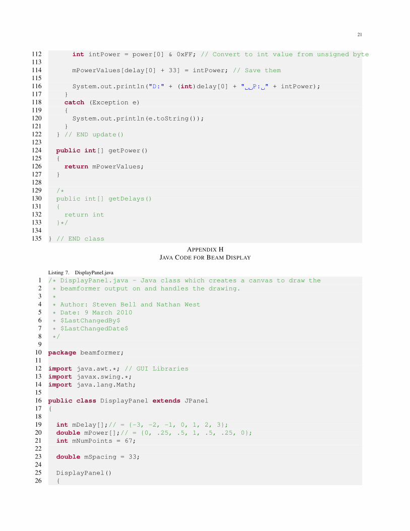
10 package beamformer;1112 //Import the DSS packages13 import com.ti.ccstudio.scripting.environment.*;14 import com.ti.debug.engine.scripting.*;1516 public class Beamformer {1718 DebugServer debugServer;19 DebugSession debugSession;2021 RTDXInputStream inStream;2223 int[] mPowerValues;2425 public Beamformer() {26 mPowerValues = new int[67]; // TODO: Change to numBeams2728 ScriptingEnvironment env = ScriptingEnvironment.instance();29 debugServer = null;30 debugSession = null;3132 try33 {34 // Get the Debug Server and start a Debug Session35 debugServer = (DebugServer) env.getServer("DebugServer.1");36 debugServer.setConfig("Z:/2010_Spring/dsp/codecomposer_workspace/dsp_project_trunk/dskboard.ccxml");37 debugSession = debugServer.openSession(".*");3839 // Connect to the target40 debugSession.target.connect();41 System.out.println("Connected to target.");4243 // Load the program44 debugSession.memory.loadProgram("Z:/2010_Spring/dsp/codecomposer_workspace/dsp_project_trunk/Debug/beamformer.out");45 System.out.println("Program loaded.");4647 // Get the RTDX server48 RTDXServer commServer = (RTDXServer)env.getServer("RTDXServer.1");49 System.out.println("RTDX server opened.");5051 RTDXSession commSession = commServer.openSession(debugSession);5253 // Set up the RTDX input channel54 inStream = new RTDXInputStream(commSession, "dataChan");55 inStream.enable();56 }57 catch (Exception e)

20

58 {59 System.out.println(e.toString());60 }61 }6263 public void start()64 {65 // Start running the program on the DSK66 try{67 debugSession.target.restart();68 System.out.println("Target restarted.");69 debugSession.target.runAsynch();70 System.out.println("Program running....");71 Thread.currentThread().sleep(1000); // Wait a second for the program to run72 }73 catch (Exception e)74 {75 System.out.println(e.toString());76 }77 }7879 public void stop()80 {81 // Stop running the program on the DSK82 try{83 debugSession.target.halt();84 System.out.println("Program halted.");85 }86 catch (Exception e)87 {88 System.out.println(e.toString());89 }9091 }9293 public void setMode()94 {9596 }9798 public void setNumBeams()99 {

100101 }102103 public void update(){104 try{105 // Read some bytes106 byte[] power = new byte[1];107 byte[] delay = new byte[1];108109 inStream.read(delay, 0, 1, 0); // Read one byte, wait indefinitely for it110 inStream.read(power, 0, 1, 0); // Read one byte, wait indefinitely for it111

21

112 int intPower = power[0] & 0xFF; // Convert to int value from unsigned byte113114 mPowerValues[delay[0] + 33] = intPower; // Save them115116 System.out.println("D:" + (int)delay[0] + " P: " + intPower);117 }118 catch (Exception e)119 {120 System.out.println(e.toString());121 }122 } // END update()123124 public int[] getPower()125 {126 return mPowerValues;127 }128129 /*130 public int[] getDelays()131 {132 return int133 }*/134135 } // END class

APPENDIX HJAVA CODE FOR BEAM DISPLAY

Listing 7. DisplayPanel.java1 /* DisplayPanel.java - Java class which creates a canvas to draw the2 * beamformer output on and handles the drawing.3 *4 * Author: Steven Bell and Nathan West5 * Date: 9 March 20106 * $LastChangedBy$7 * $LastChangedDate$8 */9

10 package beamformer;1112 import java.awt.*; // GUI Libraries13 import javax.swing.*;14 import java.lang.Math;1516 public class DisplayPanel extends JPanel17 {1819 int mDelay[];// = {-3, -2, -1, 0, 1, 2, 3};20 double mPower[];// = {0, .25, .5, 1, .5, .25, 0};21 int mNumPoints = 67;2223 double mSpacing = 33;2425 DisplayPanel()26 {

22

27 mDelay = new int[mNumPoints];28 mPower = new double[mNumPoints];2930 for(int i = 0; i < mNumPoints; i++){31 mDelay[i] = i - 33;32 mPower[i] = .5;33 }34 }3536 void updatePower(int[] newPower)37 {38 for(int i = 0; i < mNumPoints; i++)39 {40 mPower[i] = (double)newPower[i] / 255;41 if(mPower[i] > 1){42 mPower[i] = 1;43 }44 }45 this.repaint();46 }4748 static final int FIGURE_PADDING = 10;4950 // Overrides paintComponent from JPanel51 protected void paintComponent(Graphics g)52 {53 super.paintComponent(g);5455 Graphics2D g2d = (Graphics2D)g; // Cast to a Graphics2D so we can do more advanced painting56 g2d.setRenderingHint(RenderingHints.KEY_ANTIALIASING, RenderingHints.VALUE_ANTIALIAS_ON);5758 // Determine the maximum radius we can use. It will either be half59 // of the width, or the full height (since we do a semicircular plot).60 int maxRadius = this.getWidth()/2;61 if(maxRadius > this.getHeight()){62 maxRadius = this.getHeight();63 }64 maxRadius = maxRadius - FIGURE_PADDING;6566 // Pick our center point67 int centerX = this.getWidth() / 2;68 int centerY = this.getHeight()-(this.getHeight() - maxRadius) / 2;6970 // Calculate all of the points71 int[] px = new int[mNumPoints];72 int[] py = new int[mNumPoints];7374 for(int i = 0; i < mNumPoints; i++)75 {76 double angle = delayToAngle(mDelay[i]);77 px[i] = centerX - (int)(maxRadius * mPower[i] * Math.sin(angle));78 py[i] = centerY - (int)(maxRadius * mPower[i] * Math.cos(angle));79 }80

23

81 g2d.setPaint(Color.BLUE);82 g2d.drawPolygon(px, py, mNumPoints);8384 // Draw the outline of the display, so we have some context85 g2d.setPaint(Color.BLACK);86 float[] dash = {5, 4};87 g2d.setStroke(new BasicStroke((float).5, BasicStroke.CAP_BUTT, BasicStroke.JOIN_MITER, 1, dash, 0));88 g2d.drawLine(10, centerY, this.getWidth() - 10, centerY);89 g2d.drawArc(10, (this.getHeight() - maxRadius) / 2, 2*maxRadius, 2*maxRadius, 0, 180);90 }9192 // Takes a delay and converts it to the equivalent in radians93 private double delayToAngle(int delay)94 {95 return(Math.PI/2 - Math.acos(delay/mSpacing));96 }9798 // Takes an angle in radians (-pi/2 to +pi/2) and converts it to a delay99 private int angleToDelay(double angle)

100 {101 return(int)(mSpacing * Math.cos(angle + Math.PI/2));102 }103 }