ACCIONES QUE CONTRIBUYEN A LA Ó ÍESTIMACIÓN DEL PELIGRO SÍSMICO

Jorge Aguirre González, Alejandro Ramírez Gaitán, Miguel Rodríguez González, Ricardo Vázquez Rosas, Horacio Mijares Arellano y Orlando Fabela Rodríguez

ACTIONS THAT CONTRIBUTE TOTHE SEISMIC HAZARD ESTIMATION

ProbabilisticProbabilistic ApproachApproachPGA Distribution espected for a given period of time

Definition of seismogenic ZonesGround Motion Atenuation Relation

DeterministicDeterministic ApproachApproachDeterministicDeterministic ApproachApproachWaveforms from a specific earthquake scenario.

Details of Seismic Source (characterization)Details of Path.Details of Site Effect.

Framework of predicting strong ground motions for scenario Framework of predicting strong ground motions for scenario earthquakes (earthquakes (IrikuraIrikura, 2004), 2004)

1. Long-term forcasting of earthquakes

Active fault survey

2. Strong motion observation and waveform inversion of

source process

Strong motion records

3. Investigation of underground structures

Reflection and/or refraction profiling

Historical earthquake records GPS observation Seismic activity monitoring

Teleseismic records Broad-band records Earthquake damage records

Gravity survey Boring, P-S velocity loggingMicrotremor array measurement

Macroscopic (Outer)

Microscopic (Inner)

Empirical approach

StochasticTheoretical

Source modeling (Outer source parameters) (Inner source parameters)

Estimation of Green’s Function (Empirical Green’s Function) (Stochastic Green’s Function) (Theoretical Green’s Function)

Rupture directivityHybrid

Source modeling (Outer source parameters) (Inner source parameters)

Estimation of Green’s Function (Empirical Green’s Function) (Stochastic Green’s Function) (Theoretical Green’s Function)

4. Ground motion simulation for scenario earthquakes

Ground motion waveform PGA, PGV Response spectra Seismic intensity

Building codes Hospital, School, Bridge, Dam, Nuclear power plants

5. Setting seismic design criteria

Seismic intensity Nuclear power plants

Validation by historical records of earthquake damage

SITE EFFECTS

SEISMICSOURCE

SEISMIC SOURCE CHARACTERIZATION

EARTHQUAKE STRONG GROUND MOTIONS

SEISMIC SOURCE CHARACTERIZATIONINER and OUTER PARAMETERS

SEISMIC WAVES PATHGMAR

ATENUATION

LOCAL GROUND CONDITIONSLOCAL GROUND CONDITIONSSite effects

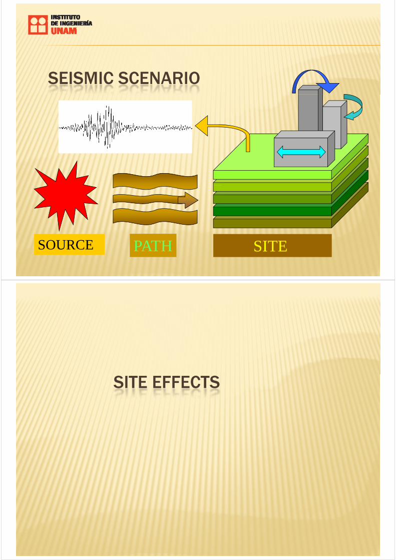
SEISMIC SCENARIO

SOURCE PATH SITE

SITE EFFECTS

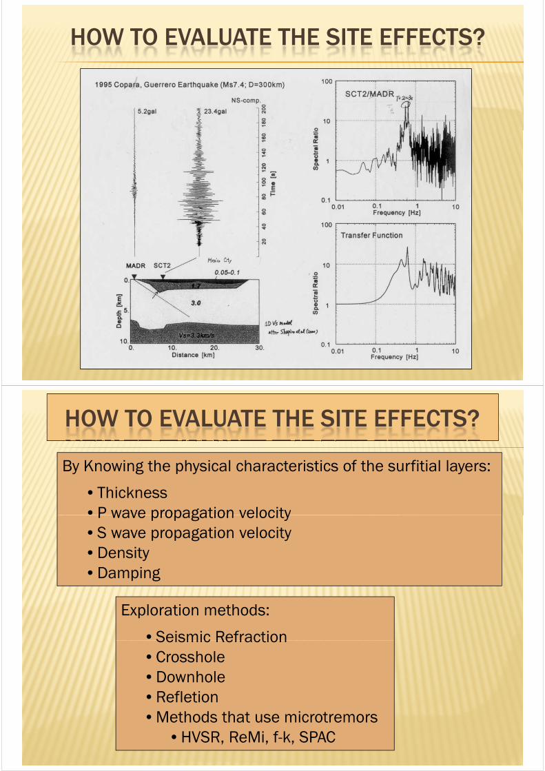
HOW TO EVALUATE THE SITE EFFECTS?

HOW TO EVALUATE THE SITE EFFECTS?

By Knowing the physical characteristics of the surfitial layers:

• Thickness• P wave propagation velocityP wave propagation velocity• S wave propagation velocity• Density• Damping

Exploration methods:

• Seismic RefractionSeismic Refraction• Crosshole• Downhole• Refletion• Methods that use microtremors

• HVSR, ReMi, f-k, SPAC

PredominantPeriod

).(.).(.

fVertCompfHorizComp

HVSR=

Uso “tradicional” de Microtremores

f=1.2 Hz

Vf

s

h=50 mVs hf

4=

Vs=240 m/s

h=100 m

Vs=480 m/sVs=120 m/s

h=25 m h

SPAC METHOD(SPATIAL AUTOCORRELATION METHOD)

Propoused by Aki (1957).Mi i i l Microtremors in instrumental arrays.Rayleigh waves phase velocity dispersion curves estimation, throughthe spatial autocorrelation.Velocity structure * At least 3 stations.

From SAGEP 2003 (corporation OYO).

SPAC METHODMICROTREMORS ARRAY OBSERVATION

SPAC method

* *

*

Ph

ase

Vlo

city v1

v2

v3

frequency (Hz)

EXAMPLES OF MICROTREMOR ARRAY OBSERVATION USING TRIANGLES

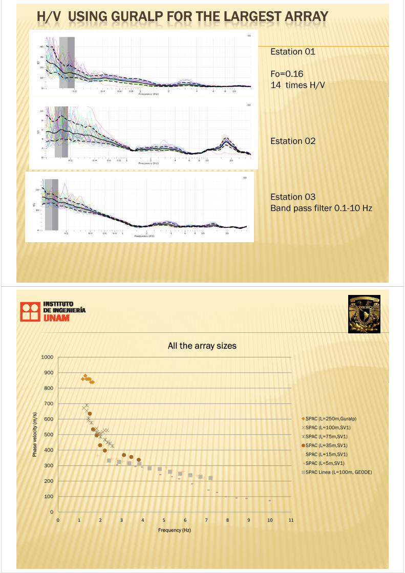
H/V USING GURALP FOR THE LARGEST ARRAY

Estation 01

Fo=0.1614 times H/V

Estation 02

Estation 03Band pass filter 0.1-10 Hz

900

1000

All the array sizes

300

400

500

600

700

800

Phas

eve

loci

ty(m

/s)

SPAC (L=250m,Guralp)

SPAC (L=100m,SV1)

SPAC (L=75m,SV1)

SPAC (L=35m,SV1)

SPAC (L=15m,SV1)

SPAC (L=5m,SV1)

SPAC Linea (L=100m, GEODE)

0

100

200

0 1 2 3 4 5 6 7 8 9 10 11

Frequency (Hz)

COMPARISON WITH THE GEOLOGICAL MODEL

APSIS: FREE SOFTWARE

FUNCTION 1: CONTROL AND RECORDING OF MOTIONS USING THE SEISMIC UNIT SR04

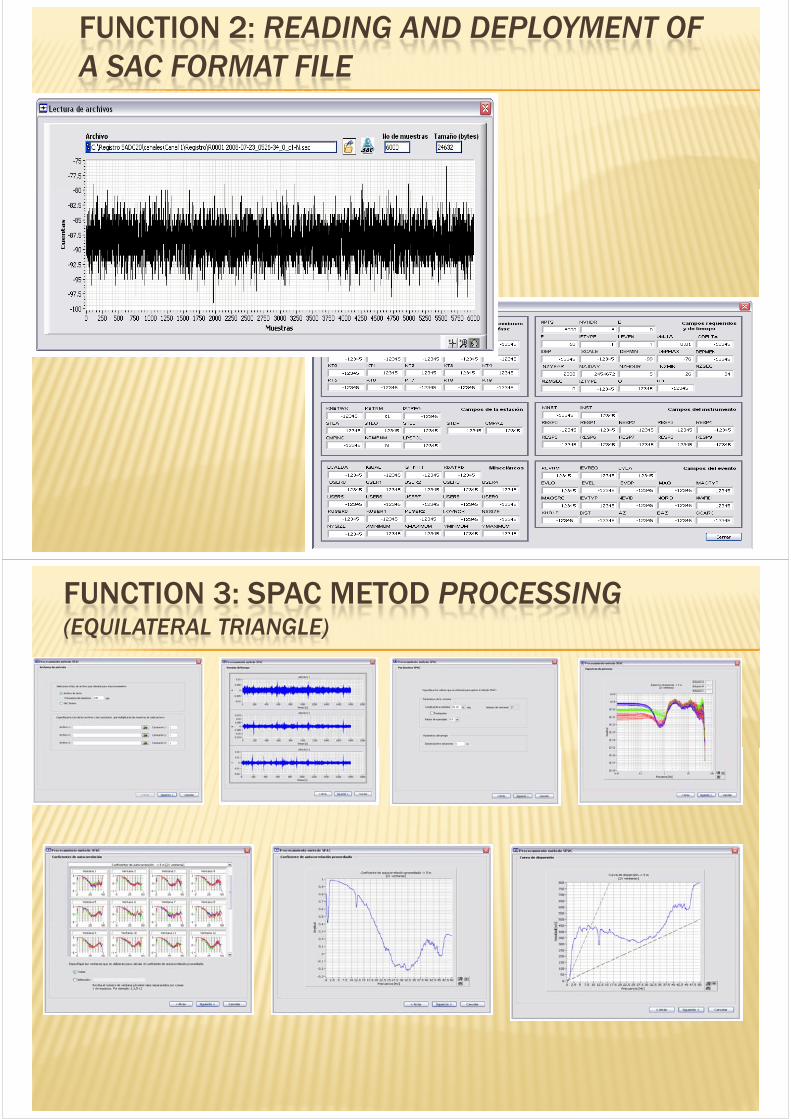
FUNCTION 2: READING AND DEPLOYMENT OF A SAC FORMAT FILE

FUNCTION 3: SPAC METOD PROCESSING(EQUILATERAL TRIANGLE)

USERUSERMANUAL

MEXICO CITY 3D MODEL

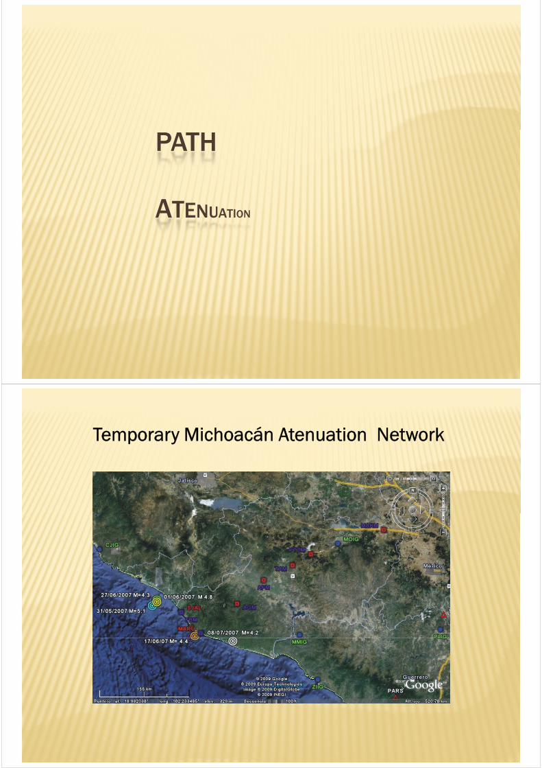
PATH

ATENUATION

Temporary Michoacán Atenuation Network

Earthquakes Analyzed in This Study

Event Date Latitude Longitude Depth Mw Mo

No (d/m/y) (°N) (°W) (Km) (dyne-cm)

1 31/05//2007 18.66 -104.14 11 5.1 5.62x1023

2 31/05//2008 18.2 -103.49 5 4.5 7.08x1022

3 06/01/2007 18.72 -104.07 20 4.8 2.00x1022

4 17/06/2007 18.22 -103.44 12 4.4 5.01x1022

5 27/06/2007 18.75 -104.07 8 4.3 3.55x1022

6 07/05/2007 18.19 -103.44 5 4.1 1.78x1022

7 07/08/2007 18.16 -102.83 16 4.2 2.51x1022

Data Analysis

Resampling

remotionmodelsource2ω remotionmodelsourceω

QUALITY FACTOR VS FREQUENCY

THIS WORK COMPARED WITH OTHERS

AMPLITUDE VS DISTANCE

REGIONAL GEOLOGY OF MICHOACAN STATE

CONCLUSIONS(ATENUATION)

• Temporary Network in Michoacán State• Temporary Network in Michoacán State• Seven eathquakes used ( 4.1 < Mw < 5.1 )• Distances from about 20 to 320 Km• Q = 105 f 0.74

• SmallerSmaller thanthan previousprevious relationsrelations forfor GuerreroGuerrero

•• NeoNeo--volcanicvolcanic transtrans--mexicanmexican beltbelt

•• RiskyRisky toto extrapolateextrapolate thethe atenuationatenuation relationsrelations

SOURCE

#ZAIIG23°N

TECOMAN EARTHQUAKE22/I/2003 MW 7.5

#

##

MOIGCJIG

MANZ19°N

20°N

21°N

22°N

#

#

^ 1̂9/11/06 06:59:07.22/01/03 02:06:34.5

ZIIG

106°W 105°W 104°W 103°W 102°W 101°W 100°W 99°W 98°W

17°N

18°N

19 N

0 200100

Kilometers

EGF METHOD APLICATIONEGF METHOD APLICATIONSmall Shock19 nov 2006Mw. 5.6# ZAIIG

0 16080

Kilometers

SOURCE MODEL

# #MOIG

CJIG

Mainshock21 enero 2003Mw. 7.6

^

#̂# #

#19/11/06 06:59:07.

22/01/03 02:06:34.5

ZIIG

MANZ

D

)(*)()( tattFr

tANx Nw

⎟⎟⎞

⎜⎜⎛

= ∑ ∑

EmpiricalEmpirical GreenGreen´́ss FunctionFunction MethodMethod

).(*)()(1 1

tattFr

tA iji j ij

−⎟⎟⎠

⎜⎜⎝

= ∑ ∑= =

Synthetic

Observed

ModelModel ValidationValidation

# ZAIIG0 16080

KilometersSynthetic

MODELOMANZ

MANZ MANZ ## #

MOIGCJIG

MANZ

Observed

MODELO MOIG

ZIIG

ZAIG

CJIGCJIG

MOIG

ZIIG

ZAIG

TheThe fivefive stationsstations usedused toto obtainobtainthethe sourcesource modelmodel..

^ ^

#19/11/06 06:59:07.

22/01/03 02:06:34.5

ZIIG

4.3a

4.3b 4.3c

SOURCE CHARACTERIZATION USING EMPIRICAL GREEN´S FUNCTIONS METHOD

#

MOIG

ZAIIG23°N

22°N

21°N

20°N

4.3d

#

##

#

^ 1̂9/11/06 06:59:07.22/01/03 02:06:34.5

ZIIG

MOIGCJIG

MANZ

98°W99°W100°W101°W102°W103°W104°W105°W106°W

19°N

18°N

17°N0 200100

Kilometros

4.3e

0 10 20 30-400

-200

0

200

400

600

800

Synthetic

Observed

Aceleration

EW

Com

p. c

m/s

/s

0 10 20 30

-20

0

20

40

60

80

Velocity

EW

Com

p. c

m/s

0 10 20 30-20

0

20

40

60

Displacement

EW

Com

p. c

m

-200

0

200

400

600

800

NS

Com

p. c

m/s

/s

20

0

20

40

60

80

NS

Com

p. c

m/s

0

20

40

60

NS

Com

p. c

m

MANZ STATION

50 100 150 200 250-10

-5

0

5

10

15

Synthetic

Observed

Aceleration

EW

Com

p. c

m/s

/s

50 100 150 200 250-2

0

2

Velocity

EW

Com

p. c

m/s

50 100 150 200 250

-1

0

1

Displacement

EW

Com

p. c

m

-5

0

5

10

15

NS

Com

p. c

m/s

/s

0

2

NS

Com

p. c

m/s

0

1

NS

Com

p. c

m

MOIG STATION

0 10 20 30-400

200

Aceleration

N

0 10 20 30

-20

Velocity0 10 20 30

-20

Displacement

0 10 20 30-400

-200

0

200

400

600

800

Aceleration

Z C

omp.

cm

/s/s

0 10 20 30

-20

0

20

40

60

80

Velocity

Z C

omp.

cm

/s

0 10 20 30-20

0

20

40

60

Displacement

Z C

omp.

cm

ZAIG STATION

50 100 150 200 250-10

5

Aceleration

N

50 100 150 200 250-2

Velocity

N

50 100 150 200 250

-1

Displacement

50 100 150 200 250-10

-5

0

5

10

15

Aceleration

Z C

omp.

cm

/s/s

50 100 150 200 250-2

0

2

Velocity

Z C

omp.

cm

/s

50 100 150 200 250

-1

0

1

Displacement

Z C

omp.

cm

0

1

2 Synthetic

Observed

EW

Com

p. c

m/s

/s

0

0.5

1

EW

Com

p. c

m/s

0

0.5

EW

Com

p. c

m

50 100 150 200 250-1

Aceleration

E

50 100 150 200 250-0.5

Velocity

E

50 100 150 200 250-0.5

Displacement

50 100 150 200 250-1

0

1

2

Aceleration

NS

Com

p. c

m/s

/s

50 100 150 200 250-0.5

0

0.5

1

Velocity

NS

Com

p. c

m/s

50 100 150 200 250-0.5

0

0.5

Displacement

NS

Com

p. c

m

50 100 150 200 250-1

0

1

2

Aceleration

Z C

omp.

cm

/s/s

50 100 150 200 250-0.5

0

0.5

1

Velocity

Z C

omp.

cm

/s

50 100 150 200 250-0.5

0

0.5

Displacement

Z C

omp.

cm

FOURIER SPECTRA STATION MANZ (3 SMGA) GREEN – SYNTETICS BLUE - OBSERVED

100

105

Aceleraciónp.

[cm

/s/s

]

100

105

Velocidad

mp.

[cm

/s]

100

105

Desplazamiento

mp.

[cm

]

100

101

10Sintético azul

Observado rojoEW

Com

p

frecuencia [Hz]10

010

1

10

EW

Com

frecuencia [Hz]10

010

1

10

EW

Com

frecuencia [Hz]

100

101

100

105

NS

Com

p. [

cm/s

/s]

100

101

100

105

NS

Com

p. [

cm/s

]

frecuencia [Hz]10

010

1

100

105

NS

Com

p. [

cm]

frecuencia [Hz]

105

105

105

100

101

100

10

frecuencia [Hz]

Z C

omp.

[cm

/s/s

]

100

101

100

10

frecuencia [Hz]

Z C

omp.

[cm

/s]

100

101

100

10

frecuencia [Hz]Z

Com

p. [

cm]

COMPARISON WITH THE DISLOCATIONMODEL OBTAINED BY YAGI ET AL. (2004).

#

#

ZAIIG

GDLC

CDGUO P ifi

Estaciones regionales y locales donde se registro el sismo de 19/11/06

# Estaciones acelerograficas del IINGEN de la UNAM

# Estaciones de banda ancha del Servicio Sismologico Nacional StationsStations wherewhere wewe simulatesimulatethethe mainshockmainshock usingusing thethesourcesource modelmodel

• 16 RTC y R Tecomán

• 2 RESCO

#BOMB

CUHA

103°51'0"W103°52'0"W103°53'0"W

55

0N

Estaciones locales donde se aplico el modelo.

# Arreglo de sismografos de banda corta Tecomán.

#

##

#

#

###

#### #

#

#

####

#

###

# #

#

##

#

#

#

##

MOIGCJIG

MANZ SJAL

MARUCALE UNIO

0 200100

Kilometros

Oceano Pacifico

#

#

COMA

EZ5

103°30'0104°0'0"W104°30'0"W

1930

0N

Estaciones locales donde se aplico el modelo.

# Arreglo de sismografos de banda corta Tecomán.

# Estaciones de RESCO

# Estaciones del IINGEN de la UNAM

# Acelerografos de la Red Temporal Costera

• 4 SSN

• 9 IINGEN

##

#

#

#TECOMAN CAMP

TXPA

INDC

CUHA

PROCO185

1854

0N

0 10.5

KilometrosOceano Pacifico

#

#

#

#

#

#

######

#

#

#

#

#

#

#

# ##

#

#

#MACE

COJU

COLLR15

ELTB, E

COL

CAMPTXPAINDCBOMB

NAR

PAR

CEOR

CIHU

TAPESE5

CENEZA

SAN

CHA CAMP

19

00

N

0 3015

Kilometros

Oceano Pacifico

SimulationsSimulations forfor stacionsstacions at rock at rock sitesite withinwithinthethe Colima Colima StateState

NS Component cm/s/s

169.1 CEN

225.3 COL

169.1 CEN

225.3 COL

EW Component cm/s/s

229.7 CEN

190.2 COL

229.7 CEN

190.2 COL

Z Component cm/s/s

129.5 CEN

59 COL

129.5 CEN

59 COL

114.3 EZ5

116.9 COLL

120 COJU

98.6 CIHU

114.3 EZ5

116.9 COLL

120 COJU

98.6 CIHU

76.5 EZ5

132.7 COLL

216 COJU

110.9 CIHU

76.5 EZ5

132.7 COLL

216 COJU

110.9 CIHU

58.4 EZ5

80.4 COLL

111.3 COJU

85.3 CIHU

58.4 EZ5

80.4 COLL

111.3 COJU

85.3 CIHU

0 10 20 30 40 50

307 TAPE

373.9 SE5

349.1 MACE

307 TAPE

373.9 SE5

349.1 MACE

0 10 20 30 40 50

335.4 TAPE

348.9 SE5

276.8 MACE

335.4 TAPE

348.9 SE5

276.8 MACE

0 10 20 30 40 50

164.6 TAPE

128.4 SE5

149.4 MACE

164.6 TAPE

128.4 SE5

149.4 MACE

SimulationSimulation forfor stationsstations soilsoil withinwithin Colima Colima StateStateNS Component cm/s/s

275.5 CAMP

219.7 CAM

228.5 BOMB

220 BA5

EW Component cm/s/s

240.5 CAMP

260.7 CAM

171.2 BOMB

171.9 BA5

Z Component cm/s/s

250 CAMP

302.2 CAM

159.9 BOMB

130.7 BA5

352.9 MANZ

226.8 INEC

123.3 EZA

376.1 CUHA

92.3 COMA

133 CHA

140.9 CEOR

375.2 MANZ

211.6 INEC

231.8 EZA

390.9 CUHA

132.9 COMA

83.6 CHA

110.3 CEOR

163.5 MANZ

203.4 INEC

126.4 EZA

223.7 CUHA

88.1 COMA

94.6 CHA

75.8 CEOR

0 10 20 30 40 50

176.4 TXPN

69.1 R15

200.6 PROCO

256.3 PAR

551.8 NAR

0 10 20 30 40 50

302 TXPN

89.5 R15

407.1 PROCO

232.2 PAR

530 NAR

0 10 20 30 40 50

358.2 TXPN

69.4 R15

121 PROCO

172.5 PAR

215 NAR

SimulationSimulation forfor stationsstations outsideoutside of Colimaof ColimaNS Componente cm/s/s

11.3 GUAD

10.5 CIIG

EW Componente cm/s/s

15.8 GUAD

14.2 CIIG

Z Componente cm/s/s

15.2 GUAD

9.1 CIIG

5.6 MOIG

36 MARU

174.6 LIMA

36.3 GZMN

4.2 MOIG

34.7 MARU

159.9 LIMA

26.9 GZMN

3.3 MOIG

24.4 MARU

151.6 LIMA

23.5 GZMN

0 50 100 150 200

1.8 ZIIG

1 ZAIG

0 50 100 150 200

2 ZIIG

0.5 ZAIG

0 50 100 150 200

2 ZIIG

0.9 ZAIG

10000

(c)

m/s

/s

1000

(d)

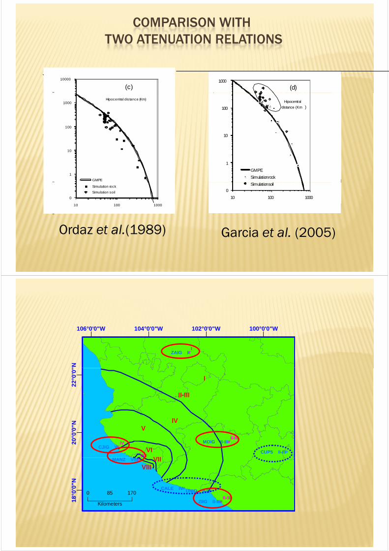
COMPARISON WITHTWO ATENUATION RELATIONS

1

10

100

1000Hipocentral dis tance (Km)

GMPE

Pea

k ac

cele

ratio

n cm

1

10

100

Hipocentral

distance (Km )

GMPE

Simulation rock

0

10 100 1000

Simulation rock

Simulation soil

Distance (km)

0

10 100 1000

Simulationsoil

Garcia et al. (2005)Ordaz et al.(1989)

##ZAIG II

100°0'0"W102°0'0"W104°0'0"W106°0'0"W

"N

##

##

#CJIG V

MOIG II-III

CUP5 II-III

IV

VIII

II-III

22°0

'0"

20°0

'0"N V

IV

II-III

I

VI

VII

##

#

#

#

#

CALE IV

MANZ VIII

ZIIG II-III

UNIO II-III

II-III18°0

'0"N

0 17085

Kilometers

VIIVIII

100°0'0"W102°0'0"W104°0'0"W106°0'0"W

0"N

Singh et al. (2003)

This study

Zobin and Pizano Silva (2008)22

°0'0

20°0

'0"N

VVI

V

IV

18°

0'0

"N

0 200100

Kilometers

VI

VIIIVII

VI

VII

V

VII

IV

CONCLUSIONS (SOURCE)

SuccesfullSuccesfull aplicationaplication of EGFMof EGFM

HighHigh frequencyfrequency modelmodel thatthat are of are of interestinterest totoearthquakeearthquake engineeringengineeringearthquakeearthquake engineeringengineering

WaveformWaveform simulationsimulation at at sitessites wherewhere therethere waswasno no seismicseismic stationstation duringduring thethe TecománTecománearthquakeearthquake..

ModelModel aplicationaplication..

1.1. AccelerationAcceleration, , VelocityVelocity ,and ,and displacementdisplacementwaveformswaveforms, Fourier , Fourier spectraspectra, PGA, I, PGA, IMMMM.

2.2. WeWe can can apliedaplied ourour knowledgeknowledge odod thethe seismicseismicsourcesource forfor thethe modelingmodeling of of futurefutureearthquakesearthquakes. .