NASA Technical Memorandum 106277

ACARA User's Manual

( t;,_.C A- T ;._- I ©6 2 7 1 ) ACARA USER'S

_A:_UAL (r'_ASA) 12_3 p

N94-II167

Unclas

Dale K. Stalnaker

Lewis Research Center

Cleveland, Ohio

G3/38 0184981

August1993

https://ntrs.nasa.gov/search.jsp?R=19940006695 2019-03-06T14:44:49+00:00Z

ACARAUser's Manual

Dale K. Stalnaker

National Aeronautics and Space Administration

Lewis Research Center

Cleveland, Ohio 44135

ACARA (Availability, Cost, And Resource

Allocation) is a computer program which analyzes

system availability, lifecycle cost (LCC), and

resupply scheduling using Monte Carlo analysis to

simulate component failure and replacement. This

manual was written to:

(i) Explain how to prepare and enter input datafor use in ACARA.

(2) Explain the user interface, menus, input

screens, and input tables.

(3) Explain the algorithms used in the program.

(4) Explain each table and chart in the output.

ACARA USER'S MANUAL

Introduction

ACARA (Availability, Cost, And Resource Allocation) is a program

for analyzing availability, lifecycle cost (LCC), and resource

scheduling. It uses a statistical Monte Carlo method to simulate

a system's capacity states as well as component failure and

repair. Component failures are modelled using a combination of

exponential and Weibull probability distributions. ACARA

schedules component replacement to achieve optimum system

performance. The scheduling will comply with any constraints on

component production, resupply vehicle capacity, on-site spares,

crew manpower and equipment.

ACARA is capable of many types of analyses and trade studies

because of its integrated approach. It characterizes the system

performance in terms of both state availability and equivalent

availability (a weighted average of state availability). It can

determine the probability of exceeding a capacity state to assess

reliability and loss of load probability. ACARA can also

evaluate the effect of resource constraints on system

availability and lifecycle cost.

ACARA interprets the results of a simulation and displays tables

and charts for the following:

Performance, i.e., availability and reliability of capacity

states.

Frequency of failure and repair.

Lifecycle cost, including hardware, transportation, andmaintenance.

Usage of available resources, including mass, volume, andmaintenance man-hours.

ACARA incorporates a user-friendly, menu-driven interface with

full screen data entry. It uses a file management system to

store and retrieve input and output datasets for system

simulation scenarios.

ACARA may be obtained from the Computer Software Management and

Information Center (COSMIC) at the University of Georgia. The

phone number is (706) 542-3265. The control number for ACARA is

#LEW-15713.

Table of Contents

Abstract .......................... 1

Introduction ........................ 2

Table of Contents ...................... 3

l_._z_-

m___L,

3.___.

Get tinq Started 5• • • • • . • • • • . • . • . • . . • •

I.i Installing ACARA and Running It from DOS ...... 5

i. 2 Using ACARA' s Menu System ............. 6

1 3 Using Help Windows 8• . • • • • • • • . • • . • • • ° .

Preparinq the Data ................... 9

2.1 Defining Block Types and Individual Blocks .... 9

2.2 Defining Relationships Between Blocks and

Subsystems .................... 9

2.3 Modelling Time-to-Failure ............. 12

2.4 Modelling Down Time ................ 13

Enterinq Data Into ACARA

3.1

3.2

3.3

3.4

3.5

3.6

3.7

3.8

............... 14

Simulation Parameters .............. 15

Cost Parameters .................. 16

Block Data Menu .................. 17

Names and Properties ............... 18

Repair Time and Personnel ............. 20

Early Failure .................. 21

Random and Wearout Failure ............ 22

Numbers ..................... 23

Age ....................... 24

Installation Times ................ 25

Nominal Quantities ................ 26

Block DiagremMenu and Redundancy ......... 27

Edit Diagram ................... 27

View Diagram ................... 29

Redundancy .................... 30

Resources Constraints ............... 31

Production .................... 32

Local Spares ................... 33

Logistics .................... 34

Resupply Cutoff .................. 34

Units and Maintenance Action Nomenclature ..... 35

Printing Input .................. 36

System Files ................... 37

Runninq ACARA Simulations ............... 38

ACARA Results 39• • • • • • • . . . ° . • • . • . • • • •

5.1 Performance 40• . . . • • • . • . . . . • . • • . •

Time at Capacity ................. 40

State Availability ................ 41

Cumulative Availability .... .......... 42

Equivalent Availability .............. 45

Overall Availability ............... 47

Reliability ................... 48Continuous State Behavior ............ 52

Printing Results ................. 53

5.2 Failure and Repair Analysis ............. 54

Failure PDF ................... 54

Failure CDF 57,,.o.Q,o.ooo,....o.

Early, Random, and Wearout Failures by Period 58

Repair PDF .................... 60

Criticality .................... 63

Accumulated Early, Random, and Wearout Failures 64

Individual Block Failure Results for a Selected

Block Type .................. 65

Failure and Repair Results by Block Type ..... 66

5.3. Lifecycle Cost (LCC) ............... 68

Hardware Cost .................... 68

Transportation Costs ............... 73

Crew Costs .................... 76

Equipment Costs .................. 79

Robotics Costs ............ ...... 82

Total Costs . . .................. 85

Overall Costs ................... 88

Block Costs .................... 91

5.4. Resource Allocations ............... 93

Depot Supply .................... 93Hardware Delivered ................ 95

Resource Usage .................. 98

5.5

5.6

Results Files ................... 114

Text Files ........... . ........ 115

Acknowledgements ...................... 116

AppendixA.

B.

C.

........................ 117

Input Windows ................... 117

Input Tables ................... 118

Displaying Output ................. 122

Index .......................... 124

4

I___. Getting Started

I.i Installing ACARA and Running It from DOS.

ACARA requires an 80386 or 80486 based microcomputer with an

80387 math coprocessor and at least 2 MB of extended memory. The

operating system must be DOS 3.3 or higher. Warning: ACARA may

conflict with RAM resident software and memory managers which

reduce DOS memory below 640 K. Such programs may have to be

disabled before running ACARA. A dot-matrix printer (e.g.,

Epson) is required to print any of the graphs in ACARA's results.

ACARA is available as either the executable code or the source

code, on either a 3.5 inch or a 5.25 inch high-density diskette.

The executable code will perform all the ACARA tasks, but it does

not allow the program to be modified. The package contains the

following files:

acara.run

apl2run.exeacara.bat

contains the ACARA program

executes acara.run

invokes the apl2run sequence from DOS

To run the executable code, enter the appropriate drive and type"ACARA"

The source code is contained in the file acara.atf, which is the

APL transfer file format. The code may be modified using an APL

editor. The IBM APL2 programming language and also several

auxiliary processors are necessary. APL2 for the PC is availablefrom:

IBM Direct

Phone 800-IBM-2468

Part Number 6242936

For more assistance, call the IBM APL Hotline: 408-463-2752.

To run the source code, copy acara.atf into the system APL2

directory. Enter APL2, using the following invocation to run the

auxiliary processors:

APL232 ap2 ap80 apl00 apl01 apl03 apl20 ap124 ap207 ap210 AT

To retrieve ACARA from-the transfer file, type the command:

")IN ACARA". To execute the program, type: "ACARA". The ACARA

Main Menu will immediately appear on the screen.

1.2 Using ACARA's Menu System

ACARA's features are accessible through its cursor-driven menu

system. This menu appears immediately after you load ACARA from

DOS. The cursor is initially at the top left corner of the

screen, indicated by the arrowhead symbols surrounding the

keyword phrase "ACARA Info"

The keywords at the top of the screen represent the following

primary groups of tasks:

ACARA Info

Gives general information about ACARA. The cursor is

located here at the beginning of the ACARA session. To read

this information, press the [Enter] key.

Input

Contains tasks involving ACARA's input, such as:

• Enter data

Interfaces for input data.

• System Files

Manages files of input data.

• Clear Input

Clears input data.

Ru/1

Simulates the current system data (Individual Mode) or a

batch of ACARA system files (Batch mode).

Results contains the following:

• Performance Results Tables

• Failure & Repair Results Tables

• Lifecycle Costs Results Tables

• Resource Allocations Results Tables

• Results Files

Loads, saves, copies and deletes results of previousACARA simulations.

• Text Files

Edits, copies and deletes ASCII files of ACARA tables.

6

QuitLets you leave ACARA. If you are using the executable code,you will return to the DOS environment. If you are usingthe source code, the Main Menu will disappear, but you willremain in the APL environment. To leave the APL

environment, type the system command ")OFF"

To move between any of these options, move the cursor to the

right or left, using the cursor keys [_] and [_].

Input, Run, and Results each has its own pull-down menu. As the

cursor moves from left to right, each pull-down menu will appear

under its keyword. The ">" symbol following a keyword indicates

that the option has a pull-down menu of sub-tasks. The arrowhead

"_" on the left side of the pulldown menu is the cursor. The

option located at the cursor is described by a phrase displayedon the second row on the screen.

For example, move the cursor to the keyword Input. The top

portion of the screen should look like Figure 1.2.1, below:

infoI Input iRunResult I0oitEnter ACARA Simulation Parameters.

_Enter data >

System Files >

Clear Input

Figure 1.2.1

Input contains three options: Enter Data, System Files, and

Clear Input. Use the [_] and [¢] cursor keys to move between

these options and the [Home] and [End] keys to jump to the top orbottom of the menu.

The options Enter data and System Files each have submenus of

tasks. To call the System Files submenu, move the cursor to this

keyword and press the [Enter] key. The top portion of the screen

will look like Figure 1.2.2, below:

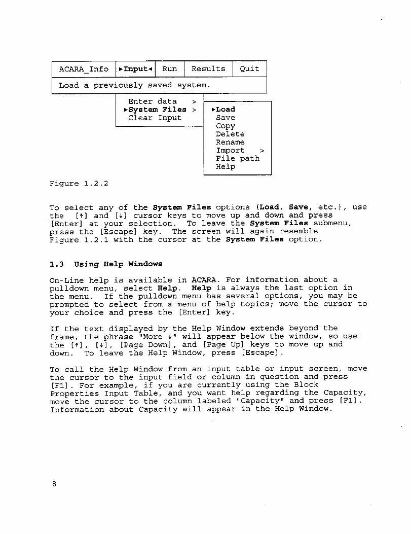
ACARA_Info l_Input_l Run Results I Quit

Load a previously saved system.

Enter data >_System Files >

Clear Input_Load

SaveCopyDeleteRenameImport >File pathHelp

Figure 1.2.2

To select any of the System Files options (Load, Save, etc.), use

the [_] and [_] cursor keys to move up and down and press

[Enter] at your selection. To leave the System Files submenu,

press the [Escape] key. The screen will again resemble

Figure 1.2.1 with the cursor at the System Files option.

1.3 Using Help Windows

On-Line help is available in ACARA. For information about a

pulldown menu, select Help. Help is always the last option in

the menu. If the pulldown menu has several options, you may be

prompted to select from a menu of help topics; move the cursor to

your choice and press the [Enter] key.

If the text displayed by the Help Window extends beyond the

frame, the phrase "More _" will appear below the window, so use

the [_], [4], [Page Down], and [Page Up] keys to move up and

down. To leave the Help Window, press [Escape].

To call the Help Window from an input table or input screen, move

the cursor to the input field or column in question and press

[FI] . For example, if you are currently using the Block

Properties Input Table, and you want help regarding the Capacity,

move the cursor to the column labeled "Capacity" and press [FI] .

Information about Capacity will appear in the Help Window.

8

2. Preparinq the Data

2.1 Defining Block Types and Individual Blocks

ACARA represents the components of a system as individual blocks.

Each block is of a certain type--each type must be given a unique

name and has characteristics (mass, volume, etc.) which

differentiate it from the others. The name of each type is

entered into the Names and Properties Input Table (page 18) as

are its mass, volume, cost, and capacity. The names will appear

at the left of each input table where other block characteristicsare defined.

Each individual block is assigned a number and is then assigned

to one of these block types, using the Block Numbers Table

(page 23).

Blocks may be installed into the system all at once or installed

in stages. In the case of staged installation, the blocks

installed during each stage are entered using the Installation

Time Input Table (page 25).

2.2 Defining Relationships Between Blocks and Subsystems

A reliability block diagram (RBD) must be prepared for ACARA to

properly simulate a system's availability. The RBD depicts a

system, which in this context is defined as an arrangement of

blocks which successfully performs a function. Each block is

either available or unavailable, i.e., there are no gradations of

partial block performance. The RBD does not necessarily depict

physical connections in the actual system, but rather shows the

role of each block in contributing to the system's function.

ACARA can model arrangements of series, parallel, or M-of-N

parallel blocks:

A series subsystem is available if all the elements it

contains are available.

A parallel subsystem is available if at least one of its

elements is available.

An M-of-N parallel subsystem is available if a specific

number of two or more parallel blocks is available. For

example, a 2-of-3 parallel subsystem contains three blocks--

at least two blocks must be available for the system to beavailable.

A simple subsystem is defined as a series or parallel combination

of two or more blocks. Subsystems can be combined further as

9

series or parallel combinations of other subsystems and/or blocksuntil the entire system is defined as a combination of subsystemsand blocks. The arrangements of blocks and subsystems arespecified by the Block Diagram Table (page 27).

ACARA has no restrictions on the total number of blocks in theRBD or the number of blocks in a series or parallel subsystem.block may appear in more than one subsystem if this isappropriate.

A

The RBD should be annotated as follows. Blocks are sequentiallynumbered as BI, B2, etc. Subsystems are numbered as SI, $2, etc.and are defined from the "inside out". A subsystem cannotcontain a subsystem of a higher number. For example, Subsystem

$3 can contain S1 and $2, but cannot contain $4. Beginning with

the innermost set of blocks, each parallel or series set of

blocks is partitioned into a subsystem which in turn may be

combined with other blocks or subsystems. The entire system is

finally described as a subsystem containing all other subsystems

and blocks.

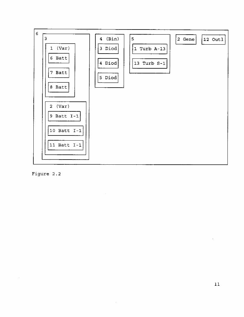
The system shown in Figure 2.2 will be used as an example

throughout this manual. The system consists of the following

components, or "blocks":

Turbine

Generator

Diode

BatteryOutlet

Blocks i, 13

Block 2

Blocks 3-5

Blocks 6-11

Block 12

The system contains 6 subsystems, as follows:

Subsystems 1 and 2 are both variable M-of-N parallel

arrangements of batteries. These subsystems respectively

contain Blocks 6 through 8 and Blocks 9 through ii.

Subsystem 3 consists of Subsystems 1 and 2 in parallel.

Subsystem 4 is a binary M-of-N parallel arrangement of

diodes, Blocks 3 through 5.

Subsystem 5 is a parallel arrangement of two turbines,

blocks 1 and 13.

Subsystem 6 comprises the entire system and is a series

arrangement of Subsystems 3 through 5 and Blocks 2 and 12.

For further information on the Block Diagram Table as well as

series, parallel, variable M-of-N and binary M-of-N subsystems,

refer to the section entitled "Edit Diagram" (page 27).

10

6

1 (Var)

6 Batt I

7 Batt I

8 Batt I

2 (Var)

19 Batt I-ll

Ii0 Batt I-i I

III Batt I-ll

4 (Bin)

3 Diod I

4 Diod I

I_o_o_I

5

II Turb A-131

2 GeneJ 12 Outl I

Figure 2.2

ii

2.3 Modelling Time-to-Failure

ACARA models the time-to-failure for each block using the Weibull

distribution function:

time-to-failure = scale x(-In R) IIs_

The shape and scale factors are adjusted to modify the form ofthe distribution. Uniform random numbers from 0 to 1 are

generated and substituted for the reliability, R. ACARA uses the

following models to generate time-to-failure: early failure

(i.e., infant mortality), random failure, and wearout failure

(i.e., life-limiting failure). These models are adjusted by

user-defined parameters to approximate the failure

characteristics of each block.

To model early failure, the mean life and shape factor are

specified for each block type and the scale factor is calculated

from the equation:

scale = mean life

Gamma(l+i/shape)

where "Gamma" is the Gamma function.

The shape factor for early failure is less than or equal to i.

The chance that a block will suffer an early failure is defined

by the Probability of Early Failure for its type. The mean life,

shape factor, and probability are entered into the Early Failure

Input Table (page 21).

Random Failure is modelled by the exponential distribution

function, a special case of the Weibull, where the shape factor

is equal to 1 and the scale is equal to the Mean Time Between

Failure (MTBF). The MTBF is entered using the Random and Wearout

Failure Input Table (page 22).

Wearout Failure is also modelled by the Weibull function. The

shape factor must be 1 or more. The wearout mean life and shape

factor are entered into the Random and Wearout Failure Input

Table. If the block is installed having an initial age (i.e., it

is not brand new), its initial age is subtracted from its first

time-to-failure due to wearout. Likewise, if it undergoes a

failure-free period, this period is added to its first time-to-

failure. Initial ages and failure-free periods are entered into

the Block Ages Input Table (page 24).

ACARA generates time-to-failure events using one or a combination

of these models and assigns the minimum resulting time for each

block as its next failure event. The early failure model is

canceled by assigning to the block type an early failure

12

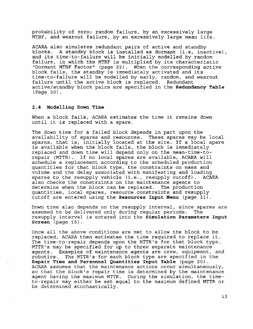
probability of zero; random failure, by an excessively largeMTBF, and wearout failure, by an excessively large mean life.

ACARA also simulates redundant pairs of active and standbyblocks. A standby block is installed as dormant (i.e, inactive),and its time-to-failure will be initially modelled by randomfailure, in which the MTBF is multiplied by its characteristic"Dormant MTBF Factor" (page 22). When the corresponding activeblock fails, the standby is immediately activated and itstime-to-failure will be modelled by early, random, and wearoutfailure until the active block is replaced. Redundantactive/standby block pairs are specified in the Redundancy Table

(Page 30).

2.4 Modelling Down Time

When a block fails, ACARA estimates the time it remains down

until it is replaced with a spare.

The down time for a failed block depends in part upon the

availability of spares and resources. These spares may be local

spares, that is, initially located at the site. If a local spare

is available when the block fails, the block is immediately

replaced and down time will depend only on the mean-time-to-

repair (MTTR). If no local spares are available, ACARA will

schedule a replacement according to the scheduled production

quantities for that block type, the constraints on mass and

volume and the delay associated with manifesting and loading

spares to the resupply vehicle (i.e., resupply cutoff). ACARA

also checks the constraints on the maintenance agents to

determine when the block can be replaced. The production

quantities, local spares, resource constraints and resupply

cutoff are entered using the Resources Input Menu (page 31).

Down time also depends on the resupply interval, since spares are

assumed to be delivered only during regular periods. The

resupply interval is entered into the Simulation Parameters Input

Screen (page 15).

Once all the above conditions are met to allow the block to be

replaced, ACARA then estimates the time required to replace it.

The time-to-repair depends upon the MTTR's for that block type.

MTTR's may be specified for up to three separate maintenance

agents. Examples of maintenance agents are crew, equipment, and

robotics. The MTTR's for each block type are specified in the

Repair Time and Personnel Quantities Input Table (page 20).

ACARA assumes that the maintenance actions occur simultaneously,

so that the block's repair time is determined by the maintenance

agent having the maximum MTTR. During the simulation, the time-

to-repair may either be set equal to the maximum defined MTTR or

be determined stochastically.

13

3__=. Enterinq Data Into ACARA

The features under the Enter Data option let you enter the input

required to run an ACARA simulation. Move the cursor right to

Input and down to Enter Data, then press [Enter]. The menu

should resemble Figure 3.

Input is entered into ACARA using Input Windows and Input Tables.

Refer to the Appendix for instructions for using these input

interfaces, such as how to get a printout or an ASCII (text) file

from the table. Whenever invalid data is entered into ACARA, a

tone will sound and ACARA will return to the error until it is

corrected.

ACARA_Info l_Input, l Run Results I Quit

Enter Simulation Parameters.

_Enter Data >

System Files >

Clear Input

,Simulation

Cost Parameters

Block Data

Block Diagram

Resources

Units & Nomen.

Print Input

Help

>

>

>

Figure 3.

14

3.1 Simulation Parameters

The ACARA Simulation Parameters Input Window (Figure 3.1)

to enter the parameters necessary to run a simulation.

is used

Simulation Parameters

Number of Runs: [ 10 ]

Duration: [ 15 ]

Resupply Interval: [ 1 ]

Period Length: [ 3

Capacity Increment: [ I0

Do you want to normalize to available System Capacity?(Y/N)

Do you want a Monte Carlo Simulation of Repair time? (Y/N)

Do you want to track failure types? (Y/N) [Y]

]

]

[Y]

[Y]

Figure 3.1

The simulation parameters are as follows:

Number of Runs

Sets the number of iterations used to characterize the

system. More accurate results and more capacity states

will be determined if more iterations are specified;

however, this is at the expense of increased computation

time.

Duration

Sets the number of years of system operation to be

simulated. The duration must be divisible by both the

period length and the resupply interval.

Period Length

Sets the time interval, in years, used in the simulation for

purposes of statistical analysis.

Resupply Interval

Sets the time interval, in years, between deliveries of

spares to the system. This period must be greater than the

resupply cutoff time to manifest spares (page 34).

Capacity Increment

Sets the increment over which capacities are "binned" to

evaluate reliability, expressed as a percentage. A smaller

increment results in more detail, but requires more

computation time.

15

Do you want to normalize to available system capacity?Indicates whether the system capacity should be scaled to

the system's current capability. Enter either "Y" or "N"

(Yes or No). If the system is installed in stages, it may

be preferable to scale the capacity.

Do you want a Monte Carlo Simulation of Repair time?

Indicates whether the Monte Carlo method should be used to

determine the elapsed time for each installation and

replacement. Enter either "Y" or "N" (Yes or No). If the

answer is "No", ACARA will use the MTTR's (mean time to

repair) associated with each block type and assign the

maximum value to all blocks of that type. The latter method

uses less computation time.

Do you want to track failure types?

Indicates whether to distinguish between early, random, and

wearout failures. Enter either "Y" or "N" (Yes or No).

Answering "No" reduces the memory requirements, but some

results tables will not be available (pages 58 and 64).

3.2 Cost Parameters

The Cost Parameters Input Window is shown on Figure 3.2. Enter

into the field labeled "Transportation" the cost per unit mass

used to calculate transportation costs. Enter into the remaining

fields the costs per hour associated with the types of

maintenance actions (i.e., Crew, Equipment, Robotics, etc.). The

units for cost and mass and the maintenance nomenclature are

arbitrary and can be changed by the user (page 35).

Cost Parameters

Transportation:

Crew:

Equipment:

Robotics:

[ 3 ] ($k/ib)

[ 80 ] ($k/hour)

[ 20 ] ($k/hour)

[ 40 ] ($k/hour)

Figure 3.2

16

3.3 Block Data Menu

The Block Data Menu, shown in Figure 3.3, contains the input

tables for entering information about each block type.

Ac_infoI_Input_IRunIResults0uitEnter Block Properties.

,Enter data >

System Files>

Clear Input

Simulation

Cost Parameters

,Block Data

Block Diagram

Resources

Units & Nomen.

Print Input

Help

Figure 3.3 Block Data Menu

,Names & PropertiesMTTR & Personnel

Early FailureRandom & Wearout

Block Numbers

Initial AgesInstallation Times

Nom. Quantities

Help

17

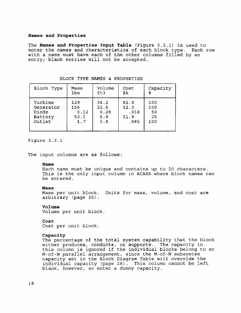
Names and Properties

The Names and Properties Input Table (Figure 3.3.1) is used to

enter the names and characteristics of each block type. Each row

with a name must have each of the other columns filled by an

entry; blank entries will not be accepted.

BLOCK TYPE NAMES & PROPERTIES

Block Type

Turbine

Generator

Diode

BatteryOutlet

Mass

ibs

129

156

0.12

53.1

1.7

Volume

ft3

34.2

22.6

0.28

6.8

0.8

Cost

Sk

82.0

12.3

.018

11.9

.085

Capacity

%

i00

i00

5O

25

i00

Figure 3.3.1

The input columns are as follows:

Name

Each name must be unique and contains up to 20 characters.

This is the only input column in ACARA where block names canbe entered.

Mass

Mass per unit block.

arbitrary (page 35).

Units for mass, volume, and cost are

Volume

Volume per unit block.

Cost

Cost per unit block.

Capacity

The percentage of the total system capability that the block

either produces, conducts, or supports. The capacity in

this column is ignored if the individual blocks belong to an

M-of-N parallel arrangement, since the M-of-N subsystem

capacity set in the Block Diagram Table will override the

individual capacity (page 28). This column cannot be left

blank, however, so enter a dummy capacity.

18

Remember that a block's capacity is by definition a

percentage of the total system capability. A "support"

block that does not contribute directly to the output, and

yet is necessary for the system to be operational, still has

a defined capacity. The capacity will depend on the

degradation in system capability resulting when the block

fails. For example, a structure that supports a battery maybe considered to be in series with that battery. It can be

assigned a capacity equal to that of the battery, since thebattery will fail whenever the structure fails. If it is

appropriate, the support block can be assigned a capacity of100%, so as not to act as a bottleneck to the RBD.

19

Repair Time and Personnel

The Repair Time and Personnel Input Table (Figure 3.3.2) is used

to enter the mean time to repair (MTTR) and the number of

personnel required for installation or maintenance of each block

type. ACARA assumes that installing a block requires as much

time and personnel as does repairing a block.

ACARA accounts for three types of maintenance agents. In the

example, they are called "Crew", "Equipment", and "Robotics"

The nomenclature is arbitrary and may be modified by the user.

(page 35)

ACARA determines the time for each maintenance agent and assumes

that the maintenance actions occur simultaneously. To account

for down time due to repair for any given block, the repair time

is estimated either by:

(i) Directly using the maximum MTTR of the three maintenance

actions. In the example system, the repair time for the

turbine will be 13.5 years, based on the Crew MTTR.

(2) Using a Monte Carlo method, i.e., the result of a Weibull

distribution about the maximum MTTR. The shape factor is

set at 3.44 to approximate a normal distribution. This

model requires more computation time.

To use the Monte Carlo method for all block types, enter 'Yes' in

the appropriate field in the Simulation Parameters Input Window

(page 15).

REPAIR TIME & PERSONNEL

Block Type

Turbine

Generator

Diode

BatteryOutlet

Crew

MTTR,Hrs No.

Crew Equipment

MTTR,Hrs

13.5 1 3.8

5.2 1 i.i

0.3 1 0

I.I 1 0.9

2.3 1 0

Equipment

No.

1

1

1

1

1

Robotics

MTTR,Hrs

0.3

0.3

0

0.3

0.3

Robotics

No.

Figure 3.3.2

2O

Early Failure

The Early Failure Input Table (Figure 3.3.3) is used to enter

data related to "infant mortality". The early failure model is

based upon the Weibull distribution function (page 12). This

distribution is adjusted by the Weibull shape and scale factors.

The scale factor is calculated using the mean life and the shapefactor.

The input columns are as follows:

Probability

The probability that the given block will suffer an early

failure. The probability must be at least 0, but no morethan I.

Mean Life

Defines the mean life, in years, for the early failuredistribution.

Shape

Defines the shape for the early failure distribution. The

shape factor must be greater than 0, but no greater than I.

EARLY FAILURE DATA

Block Type Probability Mean Life Shape

Turbine

Generator

Diode

BatteryOutlet

0

0

0.25

0.25

0

0.5

0.5

0.5

0.75

0.5

1

1

1

1

1

Figure 3.3.3

21

Random and Wearout Failure

The Random and Wearout Failure Input Table (Figure 3.3.4) is used

to enter the random and wearout failure distribution data by

block type. The input columns are as follows:

Random MTBF

The random mean-time-between-failures for active blocks, in

years, according to the exponential distribution function.

To cancel random failure for a block type, assign to it an

MTBF of 99999 years.

Dormant MTBF Factor

The factor by which to multiply the random MTBF to model

random failure for a standby block in the dormant state. In

the example system shown on page ii, Subsystem 5 is a

redundant pair of turbines, Blocks 1 and 13. Block 1 is the

active block and is assigned an MTBF of 49.2 years, while

its standby, Block 13, is initially dormant, and has an MTBF

of 492 years. If Block 1 fails, Block 13 will be activated

and its MTBF will be 49.2 years until Block 1 is replaced.

Wearout Mean Life

Defines the mean life, in years, for the wearout failure

model using the Weibull distribution function. To cancel

the wearout failure model for a block type, assign to it a

mean life of 99999 years.

Wearout Shape

Sets the shape factor for the wearout failure distribution.

The mean life and shape factor are used to calculate the

scale factor, which, along with the shape factor, adjusts

the Weibull distribution (page 12). The wearout shape

factor must be greater than or equal to i.

RANDOM & WEAROUT FAILURE DATA

Block Type

Turbine

Generator

Diode

BatteryOutlet

Random

MTBF

Years

49.2

55.8

43 .i

62.5

82.8

Dormant

MTBF

Factor

i0

1

1

1

1

WearOut

Mean Life

Years

19.8

25.6

99999

7.7

25.8

WearOut

Shape

Factor

3.44

1

1

I0

3.44

Figure 3.3.4

22

Numbers

The Block Numbers Input Table (Figure 3.3.5) assigns the type to

each block in the system. The type names, entered in the Names

and Properties Input Table, appear to the left. Block numbers

corresponding to each name are entered in the right column.

Consecutive block numbers may be signified using a dash: for

example, in Figure 3.3.5, for the diodes, ACARA interprets the

notation '3-5' as 'Blocks 3, 4, and 5.'

If the space needed exceeds the available column width, press

[F2] to call the menu and select Insert to insert blank rows (See

Appendix, page 120).

BLOCK TYPES & BLOCK NUMBERS

Block Type Block Identifier Numbers

Turbine

Generator

Diode

BatteryOutlet

1 13

2

3-5

6-11

12

Figure 3.3.5

23

Age

The Block Age Table (Figure 3.3.6) assigns initial ages to

individual blocks which are not "brand new" when they are

installed. To properly account for the age of such a block, its

initial age is subtracted from its time-to-first-failure

determined by the wearout failure model. The early failure and

random failure models do not account for initial age.

The Initial Age is also used to indicate any blocks which have a

"failure-free" period at their installation. In this case, the

failure free period is entered as a negative number. During the

simulation, the failure free period is added to the time-to-

first-failure so to properly account for the initial period

during which the block will not experience failure by the wearout

model.

Enter the block ages and the corresponding block numbers into the

left and right columns. Any block whose number is not entered

into this table is assumed to be brand new (i.e., Initial

Age = 0 years) when it is installed.

Consecutive block numbers may be indicated using a dash as in the

Block Numbers Screen. If more space is needed, use the Insert

feature (See Appendix, page 120).

BLOCK AGES AT BEGINNING OF SIMULATION

Age, Years Block Numbers

2 2

Figure 3.3.6

24

Installation Times

The Block Installation Time Table (Figure 3.3.7) assigns

installation times to blocks that have not been installed at the

beginning of the simulation. This will be the case if the system

is constructed in stages. Any such block will be initially

assigned a capacity of zero and will not contribute to the

capacity of the system until it is installed at the time

indicated by this table.

Enter the installation years and the corresponding block numbers

into the left and right columns. Any blocks not entered will be

assumed to be installed at year zero.

Consecutive block numbers may be indicated using a dash. If more

space is needed, use the Insert feature (See Appendix, page 120).

BLOCK INSTALLATION TIMES

Installation

Time, yrs

Block Numbers

9-11

Figure 3.3.7

25

Nominal Quantities

This table shows the quantities of each block type installed

during each year as indicated by the Installation Times input

table, assuming no constraints on spares and negligible

installation time. Note that this is not an input table.

Block Quantities at Each Installation Time

Block Types

Resupply Period

0 1

!Turbine I 2 0

Generator I 1 0

Diode 3 0

Battery 3 3

Outlet 1 0

Figure 3.3.8

26

3.4 Block Diagram Menu and Redundancy

The Block Diagram Menu (Figure 3.4) defines the relationships of

blocks and subsystems within the system and defines pairs ofredundant blocks.

I I

ACARA_Info l,Input, I Run Results Quit

Edit Block Diagram Table.

-Enter data •

System Files>

Clear Input

Simulation

Cost Parameters

Block Data

,Block Diagram

Resources

Units & Nomen.

Print Input

Help

Figure 3.4

>

,Edit Diagram

View Diagram

Print Diagram

Redundancy

Help

Edit Diagram

The Block Diagram Table defines arrangements of individual blocks

and subsystems. Refer to Figure 3.4.1. The input columns are asfollows:

Subsystem#

Identifier number for each subsystem.

unique and in numerical order.

The numbers must be

Type

There are four possible subsystem types (Use either upper orlower case:

Series (S)

A series subsystem is available if all the elements it

contains are available.

Parallel (P)

A parallel subsystem is available if at least one of

its elements is available.

27

Variable M-of-N Parallel (V)

An M-of-N parallel system is available if a specified

number of two or more parallel blocks are available.

M-of-N arrangements can only comprise blocks, they

cannot contain any subsystems. A variable arrangement

will decrease its capacity as each block fails. The

capacity is zero when all of the blocks in the

subsystem are down.

Binary M-of-N Parallel (B)

A binary arrangement is available at its specified

capacity only if a specified minimum number of the

blocks it contains are available. The capacity is zeroif this minimum is not met.

Elements

Identifier numbers for the blocks or subsystems contained in

each subsystem. Block numbers are preceded by the letter

"b" and subsystems by "s". Either upper or lower case are

acceptable. A block number may be repeated in two or more

different subsystems. Consecutive numbers may be indicated

by a dash. If the space needed exceeds the column width,

press [F2] to call the menu and select the Insert feature

(Refer to the Appendix, page 120).

The following two columns, Minimum # and Capacity, pertain

only to Variable and Binary M-of-N subsystems:

Minimum #

Enter the number of blocks that must be available for the

entire arrangement to be available.

Capacity

Variable: Enter the possible capacity values for the

subsystem. An M-of-N subsystem is available at the

first capacity in this set when M or more blocks are

available. It is available at the second capacity when

(M-l) blocks are available, and so on to the last

capacity level, which occurs when only one block isavailable.

Binary: Enter the percent capacity the subsystem will

support when all of its blocks are available. It is at

0% capacity when any block is not available.

28

BLOCK DIAGRAMTABLE

Sub-sys#

1

2

3

4

5

6

Type

v

v

Pb

Ps

Elements

b6-8

b9-11

sl 2

b3-5

bl 13

s3 4 5 b2 12

M-of-N data

Min# Capacity

3

3

50 40 25

50 40 25

I00

Figure 3.4.1

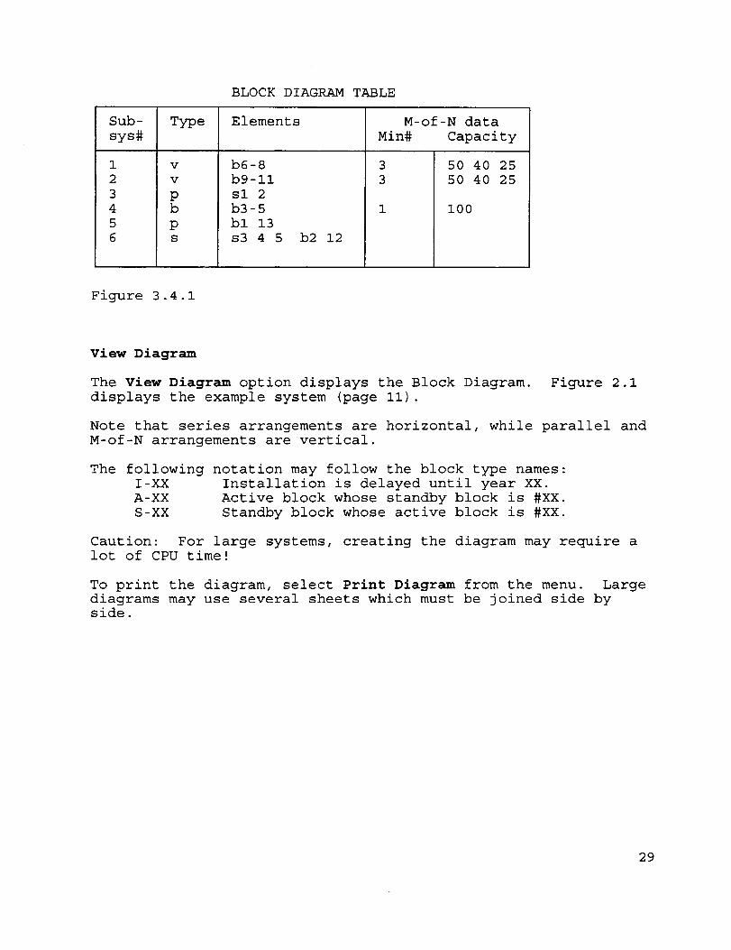
View Diagram

The View Diagram option displays the Block Diagram.

displays the example system (page Ii).

Figure 2.1

Note that series arrangements are horizontal, while parallel and

M-of-N arrangements are vertical.

The following notation may follow the block type names:

I-XX Installation is delayed until year XX.

A-XX Active block whose standby block is #XX.

S-XX Standby block whose active block is #XX.

Caution: For large systems, creating the diagram may require a

lot of CPU time!

To print the diagram, select Print Diagram from the menu. Large

diagrams may use several sheets which must be joined side byside.

29

Redundancy

The Redundancy Table specifies pairs of active and standby blocks

(See Figure 3.4.3). A standby block is operational when it is

installed, but is dormant. Its useful life will be determined

only by the exponential distribution (i.e., random failure). Its

dormant MTBF will be the product of its random MTBF and its

"Dormant MTBF Factor" (page 22). When the active block fails,

the standby is immediately activated, and will fail according to

the normal rules of early, random and wearout failure. The

standby will return to the dormant state when the active block is

repaired.

For each redundant pair of blocks, enter the number for theactive block into the left column and the number for the

corresponding standby block into the right column. An active

block can have only one standby block and vice versa. In the

example below in Figure 3.4.3, Block 13 is a standby for Block i.

To specify a system that has no redundant block pairs, enter

zeroes into the left and right columns.

Redundant Blocks

Active

Block#

1

Standby

Block#

13

Figure 3.4.3

30

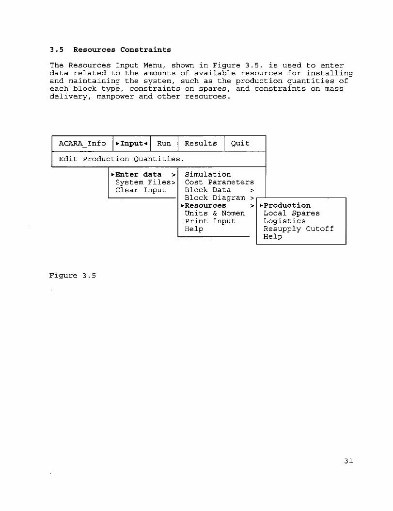
3.5 Resources Constraints

The Resources Input Menu, shown in Figure 3.5, is used to enter

data related to the amounts of available resources for installing

and maintaining the system, such as the production quantities of

each block type, constraints on spares, and constraints on mass

delivery, manpower and other resources.

Ac_intoI_Input_lRunIResultsQuitEdit Production Quantities.

,Enter data >

System Files>

Clear Input

Simulation

Cost Parameters

Block Data >

Block Diagram >

,Resources >

Units & Nomen

Print Input

Help

,Production

Local Spares

Logistics

Resupply Cutoff

Help

Figure 3.5

31

Production

The Production Quantities Table (Figure 3.5.1) is used to enter

the quantity of each block type fabricated at each period. These

blocks are available for installation and for replacement.

This input table may extend beyond the right edge of the screen.

To scroll the table to the right or left, press [Ctrl-Right] or

[Ctrl-Left], or select the Go to Column option from the Input

Table Menu.

To copy the values from a column to each column to the right,

move the cursor to that column, select Copy Column from the Input

Table Menu, and press [Enter].

In the example below, the production quantity during period I0

through to the end of the duration is 0 for each block type.

Production Quantities

Resupply Period

Block Type 0 1 2 3 4 5 6 7 8 9

Turbine 3 0 0 0 0 0 0 0 0 0

Generator 2 0 0 0 0 0 0 0 0 0

Diode i0 0 0 0 0 0 0 0 0 0

Battery 3 3 0 0 0 0 3 3 0 0Outlet 3 0 0 0 0 0 0 0 0 0

Figure 3.5.1

32

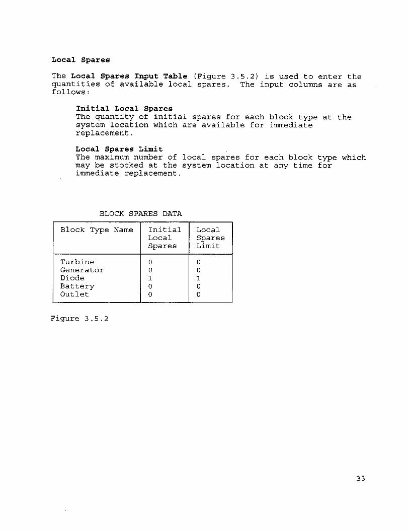
Local Spares

The Local Spares Input Table (Figure 3.5.2) is used to enter the

quantities of available local spares. The input columns are asfollows:

Initial Local Spares

The quantity of initial spares for each block type at the

system location which are available for immediate

replacement.

Local Spares Limit

The maximum number of local spares for each block type which

may be stocked at the system location at any time for

immediate replacement.

BLOCK SPARES DATA

Block Type Name

Turbine

Generator

Diode

BatteryOutlet

Initial

Local

Spares

0

0

1

0

0

Local

SparesLimit

0

0

I

0

0

Figure 3.5.2

33

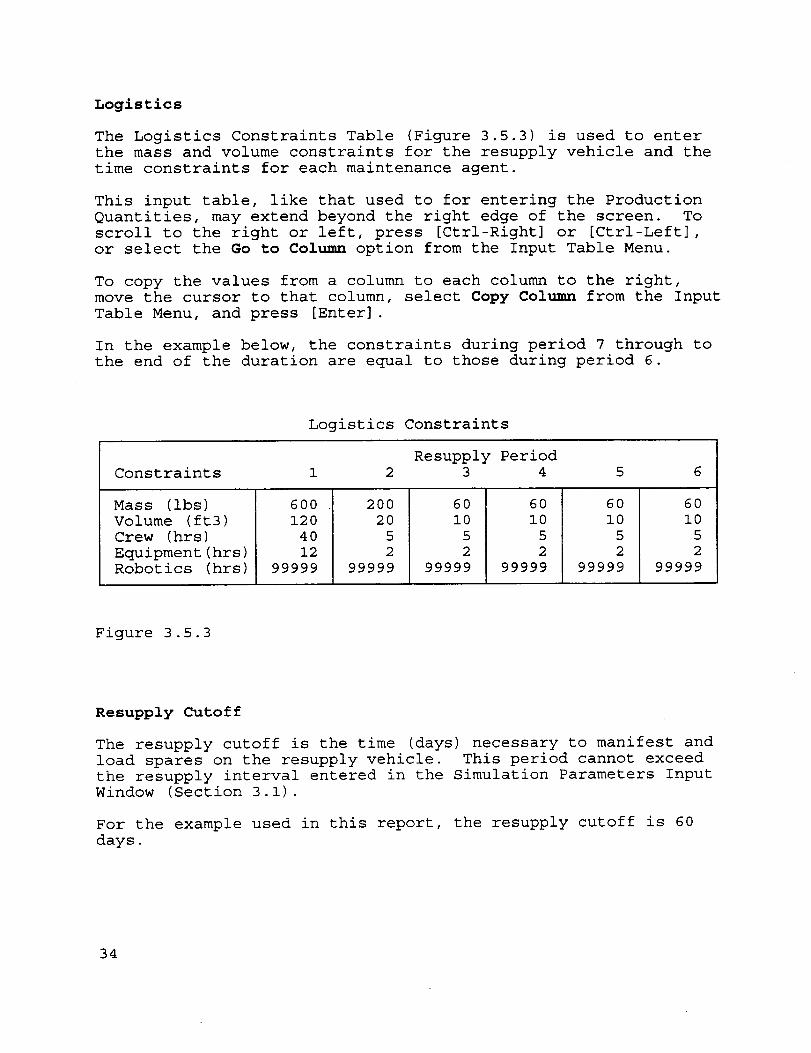
Logistics

The Logistics Constraints Table (Figure 3.5.3) is used to enter

the mass and volume constraints for the resupply vehicle and the

time constraints for each maintenance agent.

This input table, like that used to for entering the Production

Quantities, may extend beyond the right edge of the screen. To

scroll to the right or left, press [Ctrl-Right] or [Ctrl-Left],

or select the Go to Column option from the Input Table Menu.

To copy the values from a column to each column to the right,

move the cursor to that column, select Copy Column from the Input

Table Menu, and press [Enter].

In the example below, the constraints during period 7 through to

the end of the duration are equal to those during period 6.

Logistics Constraints

Resupply Period

Constraints 1 2 3 4 5 6

Mass (Ibs)

Volume (ft3)

Crew (hrs)

Equipment (hrs)

Robotics (hrs)

600

120

40

12

99999

200

20

5

2

99999

60

i0

5

2

99999

60

i0

5

2

99999

60

i0

5

2

99999

60

i0

5

2

99999

Figure 3.5.3

Resupply Cutoff

The resupply cutoff is the time (days) necessary to manifest and

load spares on the resupply vehicle. This period cannot exceed

the resupply interval entered in the Simulation Parameters Input

Window (Section 3.1).

For the example used in this report, the resupply cutoff is 60

days.

34

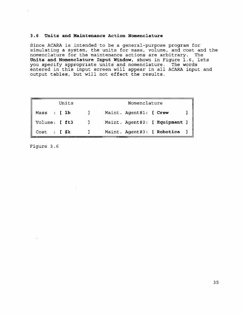
3.6 Units and Maintenance Action Nomenclature

Since ACARA is intended to be a general-purpose program for

simulating a system, the units for mass, volume, and cost and the

nomenclature for the maintenance actions are arbitrary. The

Units and Nomenclature Input Window, shown in Figure 1.6, lets

you specify appropriate units and nomenclature. The words

entered in this input screen will appear in all ACARA input and

output tables, but will not effect the results.

Units

Mass : [ ib ]

Volume: [ ft3 ]

Cost : [ Sk ]

Nomenclature

Maint. Agent#l:

Maint. Agent#2:

Maint. Agent#3:

[ Crew ]

[ Equipment ]

[ Robotics ]

Figure 3.6

35

3.7 Print Input

Use the Print Input feature for batch printouts of the current

input data. The input window on Figure 3.7 will appear. In each

field, enter the number of copies (up to 9) you want of each

input table.

Individual tables can also be printed while editing the data. To

make a printout, press [F2] and select the Print option from the

Input Table Menu.

Input Printouts

Simulation & Cost Parameters [0]

Block Properties [1]

Early Failure Data [0]

Block Types & Numbers [0]

Installation Times [0]

Block Diagram [0]

Production Quantities [0]

Logistics Constraints [0]

MTTR Data [0]

Random & Wearout Failure [0]

Initial Ages [0]

Nominal Inst. Times [0]

Redundancy Table [0]

Spares Data [0]

Figure 3.7

36

3.8 System Files

ACARA input data is stored in "system files" for future analysis.

You can load, save, copy, delete, and rename these files using

the System Files menu. The menu is also used to import system

files from ETARA (an older simulation program, similar to ACARA).

Load

Retrieves previous ACARA input from a system file. The

screen displays each file's descriptive name, size, and

creation date. To see the DOS names, press [F3]. Move the

cursor to the desired file and press [Enter] to load the

file, or [Escape] to return to the Main Menu without loadinga file.

Save

Saves the current data into a system file. You will be

prompted to enter 50-character phrase to describe the file.

Use [Page Up] and [Page Down] to scroll up and down to see

each file. Enter the descriptive name and press [Enter].

The DOS name for the system file is an abbreviation of the

description, with the extension ".asl" Press [Escape] to

return to the Main Menu without saving data.

Copy

Copies a system file. Move the cursor to your selection and

press [Enter]. At the prompt, enter a name for the copy and

press [Enter] again. To cancel and return to the Main Menu,

press [Escape].

Delete

Erases a system file. Move the cursor to a file you want to

delete and press the [Enter] key. To return to the Main

Menu, press [Escape].

Rename

Changes the descriptive name of a system file. Move the

cursor to the file you want to rename, press [Enter], and

enter a new name at the prompt. Press [Enter] again. To

cancel and return to the Main Menu, press [Escape].

Import

Retrieves data from an ETARA system file. Move the cursor

to the ETARA file you want to retrieve and press [Enter].

Only the DOS names will be visible on the screen.

File Path

Changes the file drive for system files. At the prompt,

type the appropriate file drive designation letter and press

[Enter].

37

4. Runninq ACARA Simulations

ACARA simulates systems by either Immediate Mode or Batch Mode.

Immediate

Simulates the data currently entered into ACARA. ACARA will

perform the amount of iterations entered into the Simulation

Parameters Input Screen. To stop the simulation early,

press [Escape].

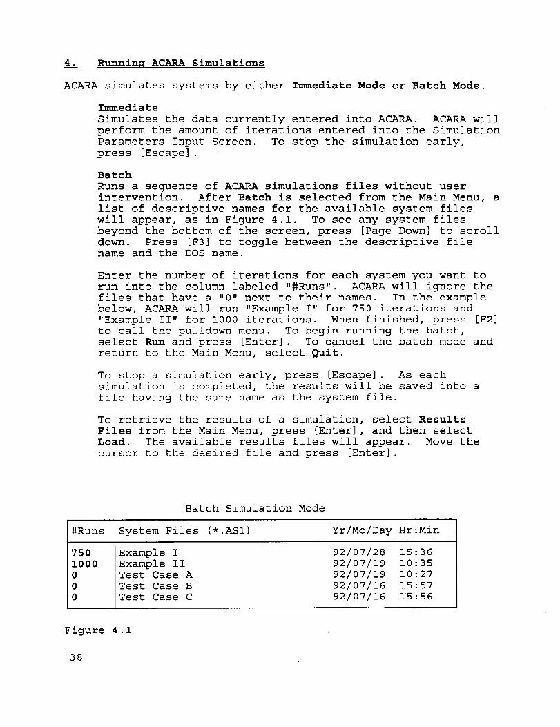
Batch

Runs a sequence of ACARA simulations files without user

intervention. After Batch is selected from the Main Menu, a

list of descriptive names for the available system files

will appear, as in Figure 4.1. To see any system files

beyond the bottom of the screen, press [Page Down] to scroll

down. Press [F3] to toggle between the descriptive file

name and the DOS name.

Enter the number of iterations for each system you want to

run into the column labeled "#Runs" ACARA will ignore the

files that have a "0" next to their names. In the example

below, ACARA will run "Example I" for 750 iterations and

"Example II" for i000 iterations. When finished, press [F2]

to call the pulldown menu. To begin running the batch,

select Run and press [Enter]. To cancel the batch mode and

return to the Main Menu, select Quit.

To stop a simulation early, press [Escape]. As each

simulation is completed, the results will be saved into a

file having the same name as the system file.

To retrieve the results of a simulation, select Results

Files from the Main Menu, press [Enter], and then select

Load. The available results files will appear. Move the

cursor to the desired file and press [Enter].

Batch Simulation Mode

#Runs System Files (*.AS1) Yr/Mo/Day Hr:Min

750

i000

0

0

0

Example I 92/07/28 15:36

Example II 92/07/19 10:35

Test Case A 92/07/19 10:27

Test Case B 92/07/16 15:57

Test Case C 92/07/16 15:56

Figure 4.1

38

5. ACARA Results

To see the results of an ACARA simulations, move the cursor to

Results at the top of the screen. The pulldown menu classifies

the results into the following groups of tables:

Performance

Describes the availability of capacity states.

Failure and Repair

Shows the frequency of failures and replacements of blocks

in the system as well as downtime and delays.

Lifecycle CostShows the maintenance cost over time.

Resource Allocations

Shows the scheduling of resupply deliveries and usage ofmaintenance time.

Each of these tables has a menu which lets you control the

printer, create text files, or view a graph. Refer to Appendix C

for further instructions.

The results examples appearing in this report correspond to the

example input shown in each of the figures in Section 3. The

input tables for Production Quantities and Logistics Constraints

(See pages 32 and 34) are each assumed to have the same values

from the time period at the column furthest to the right of the

table to the end of the duration.

In addition to the tables, the menu also has the following

options:

Computation Time

Displays the time required for ACARA to calculate theresults.

Results Files

Loads, saves, copies, renames, and deletes ACARA results

files.

Text Files

Edits, copies, renames, and deletes text (ASCII) files.

39

5.1 Performance

Time at Capacity

Table 5.1.1 displays the capacity states attained by the system

during the simulation and the amount of time the system had been

operating at each state• The left hand column shows the capacity

levels• The top row of the table shows the time periods. The

column on the far right side of the bottom section shows the

total time at each capacity state. The bottom row (entitled

"Sums") shows the total amount of time for each period.

Time at Capacity

(Normalized to Installed Capacity)

Period

Capacity 1 2 3 4 5 Overall

100 00

90 00

88 89

86 67

83 33

80 00

75 00

72 22

66 67

65 00

55 56

50 00

40.00

25.00

.00

.906

.i00

.232

.000

.326

.221

.040

.573

.000

060

131

245

000

000

166

.300

•072

.600

.000

.300

.336

.000

.300

000

300

000

000

000

000

792

574

228

096

O0O

112

299

289

.000

000

067

000

000

075

000

1 259

000

213

00O

000

00O

205

396

0O0

000

345

000

102

.106

.079

1.555

.000

217

000

000

000

037

083

000

0O0

981

000

O58

073

045

1 506

1.780

.830

.927

.000

.738

1.098

.809

.873

.000

1.752

.131

.405

.253

.125

5.278

Sums 3.000

Table 5.1.1

3.000 3.000 3.000 3.000 15.000

4O

State Availability

Table 5.1.2 displays the capacity states attained by the system

and the fraction of time the system had been operating at that

state during each period. The column on the far right side of

the bottom section shows the fraction of the total duration that

the system had attained each capacity state.

Availability of Each Capacity State

(Normalized to Installed Capacity)

Period

Capacity 1 2 3 4 5 Overall

100 00

90 00

88 89

86 67

83 33

80 00

75 00

72 22

66 67

65 00

55 56

50 00

40 00

25 00

00

.302

033

077

000

109

074

013

191

000

020

044

082

000

000

055

.i00

024

200

000

I00

112

000

I00

000

I00

000

000

000

000

264

191

076

032

000

037

i00

096

000

000

022

000

O0O

025

000

420

000

071

0O0

000

000

068

132

000

000

115

000

034

035

026

518

000

072

000

000

000

012

028

000

000

327

O00

019

024

015

5O2

.119

.055

.062

.000

049

073

054

O58

000

117

009

027

017

O08

352

Sums 1.000

Table 5.1.2

1.000 1.000 1.000 1.000 1.000

41

Cumulative Availability

Table 5.1.3 displays the fraction of time that the system has

attained a capacity state equal to or greater than the capacity

on the left-hand column. The column on the far right, labeled

"Overall" is the total fraction of the duration that the system

has attained a capacity in excess of that capacity state.

Availability of Capacity State or Greater

(Normalized to Installed Capacity)

Capacity

Period

1 2 3 4 5 Overall

i00 00

90 00

88 89

86 67

83 33

80 00

75.00

72.22

66.67

65.00

55.56

50.00

40.00

25.00

.00 1

.302

335

413

413

521

595

609

80O

8OO

819

863

945

945

945

000

i00

124

324

324

424

536

536

636

636

736

736

736

.736

.736

1.000

191

267

299

299

337

436

533

533

533

555

555

555

58O

58O

1 000

000

071

071

071

071

139

271

271

271

386

386

420

455

482

1 000

000

072

072

072

072

084

112

112

112

439

439

459

483

498

1 000

119

174

236

236

285

358

412

470

470

587

596

623

640

648

1 000

Table 5.1.3

Two graphs are associated with the Cumulative Availability table:

System Availability

Figure 5.1.3a is a graph of overall system capacity versus

availability over the entire duration. The axes are

normalized with 1.0 corresponding to 100%.

System Availability (for a Specified Period)

Figure 5.1.3b is a graph of capacity that the system

operated at or above versus the availability, during a

period specified by the user.

42

.m,I

J

,I,,Iwl

I

tI

I

I

IJ

4I

ODO0

O0

43

',,,,-I

t,.,}

_-"_¢,.)

t,,., J'J_ _.,

"."

Et-,.

,,,_,,,,.

_--:.

N

_D

ii

,el

C,_N

44

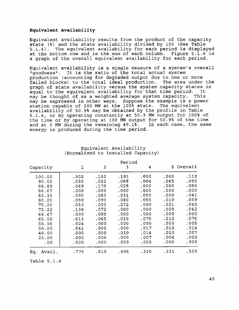
Equivalent Availability

Equivalent availability results from the product of the capacity

state (%) and the state availability divided by I00 (See Table

5.1.4). The equivalent availability for each period is displayed

at the bottom row and is the sum of each column. Figure 5.1.4 is

a graph of the overall equivalent availability for each period.

Equivalent availability is a single measure of a system's overall

"goodness". It is the ratio of the total actual system

production (accounting for degraded output due to one or more

failed blocks) to the total ideal production. The area under the

graph of state availability versus the system capacity states is

equal to the equivalent availability for that time period. It

may be thought of as a weighted average system capacity. This

may be expressed in other ways. Suppose the example is a power

station capable of i00 MW at the 100% state. The equivalent

availability of 50.9% may be obtained by the profile in Table

5.1.4, or by operating constantly at 50.9 MW output for 100% of

the time or by operating at I00 MW output for 50.9% of the time

and at 0 MW during the remaining 49.1%. In each case, the same

energy is produced during the time period.

Equivalent Availability

(Normalized to Installed Capacity)

Period

Capacity 1 2 3 4 5 Overall

I00.00

90.00

88.89

86.67

83 33

80 00

75 00

72 22

66 67

65 00

55 56

50 00

40 00

25 00

00

.302

030

069

000

O9O

059

010

138

000

013

024

041

000

000

000

I00

022

178

000

083

09O

000

072

.000

.065

.000

.000

.000

.000

.000

.191

068

028

000

031

O8O

072

000

000

015

000

000

010

000

000

.000

.064

.000

.000

000

O55

099

000

000

075

000

017

014

007

000

.000

.065

.000

.000

.000

.010

021

000

000

212

0OO

010

010

0O4

000

.119

.050

.055

.000

.041

059

040

042

000

076

OO5

014

007

002

0O0

Eq. Avail.

Table 5.1.4

.776 .610 .496 .330 .331 .5O9

45

,i.1

•.', ID

IE

I

C,

N

:-±-±_--±_+--±_±-

I I I

0

G¢'0

I.l

_N

46

Overall Availability

Table 5.1.5 displays the overall availability results. These are

the same values as in the columns on the far right side of each

of Tables 5.1.1 through 5.1.4, entitled "Overall"

SYSTEM CAPACITIES AND AVAILABILITIES

(Normalized to Installed Capacity)

System

Capacity

State

I00.00

90.00

88.89

86.67

83.33

80.00

75.00

72.22

66.67

65.00

55.56

50.00

40.00

25.00

.00

Totals:

Time @

Capacity

State, Yrs.

1.780

.830

.927

.000

.738

1.098

.809

.873

.000

1.752

.131

.405

.253

.125

5.278

15.000

Avail• of

Capacity

State

.119

.055

.062

.000

.049

.073

.054

.058

.000

.117

.009

.027

•017

.008

.352

1.000

Avail. of

Cap. State

or Greater

.119

.174

.236

.236

.285

.358

.412

.470

.470

.587

.596

.623

.640

.648

1.000

Equivalent

Availability

.119

.050

.055

.000

.041

.059

.040

.042

.000

.076

.005

.014

.007

.002

.000

.509

Table 5.1.5

47

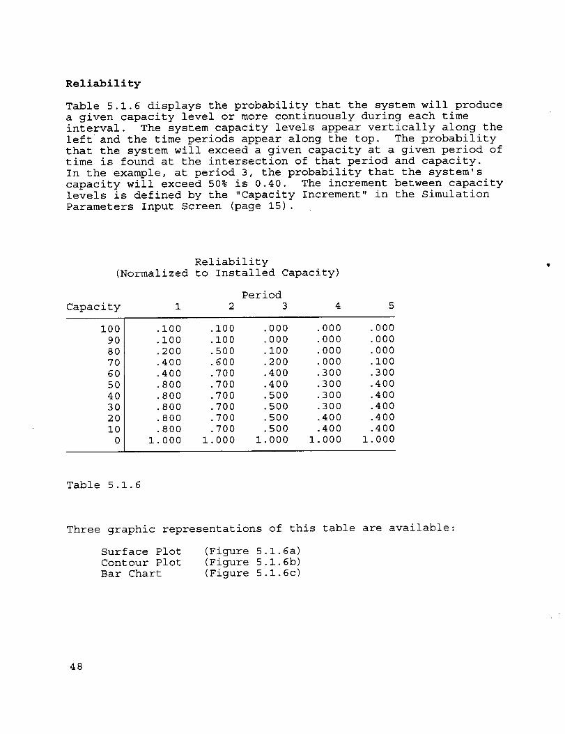
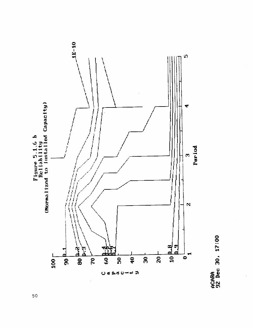
Reliability

Table 5.1.6 displays the probability that the system will produce

a given capacity level or more continuously during each time

interval. The system capacity levels appear vertically along the

leftand the time periods appear along the top. The probability

that the system will exceed a given capacity at a given period of

time is found at the intersection of that period and capacity.

In the example, at period 3, the probability that the system's

capacity will exceed 50% is 0.40. The increment between capacity

levels is defined by the "Capacity Increment" in the Simulation

Parameters Input Screen (page 15).

Reliability

(Normalized to Installed Capacity)

Capacity

Period

1 2 3 4 5

I00

90

8O

70

60

5O

40

30

20

I0

0 1

.I00

.I00

.200

400

400

8OO

8OO

8OO

80O

8OO

000

.i00

i00

5OO

600

700

700

700

.700

.700

.700

1.000

000

000

i00

200

400

400

5OO

5OO

5OO

5OO

000

00O

0OO

000

OO0

300

300

300

300

400

400

1 000

.000

000

0OO

i00

300

400

400

400

400

400

1 000

Table 5.1.6

Three graphic representations of this table are available:

Surface Plot

Contour Plot

Bar Chart

(Figure 5.1.6a)

(Figure 5.1.6b)

(Figure 5.1.6c)

48

m

w m,.# ,w

_TT_L

"m

m

;. __ __ I

. IIf"w _

i.---- I

#, _-t

I ----- I

'1--

| .. ,i (_ .--'"

ti --'_ /: l_ II _-,'"

i l"

-.l,,.

__---____--- i

l

I

._'_ ._

i_ ,_I

,...'{ ,'_ /\ "-

i I tt i Ii I I

:< 7: _ N

....." "-,.. i.."t', \..."...... ,,__t_..- '-, s .<.,/ _,

,-" ."" ;ll _J ".'" ;_._._'..... I II I I /l 1 _, ql_-' I ..---$_:* 11 iI

/.-.... ......! .. "' "":-. ,'" T

..-" .- "-.

, ,:..- _,r".,.., j.>.......... " f

if .." ...." "-.. . ..-" !,i';;'-' """ -"",.. ..

i "--.. |' iIi1

iI".'a.. I ,J"

.... ; /.-

_"" ---" i .1_

- f _t

I

N

Iot

(

' I ' I ' i

00=.

p,.

0

U

49

:h,la

{.)

{J

• .%IiI wi_

° ,-.i,laI.I'J-,',e:

£f.0T_i _

I

w-I

I

\

I

\!

r_

1.1

_N<I:{_

5O

!

00

p-

0_n

u

_t4

o c,

51

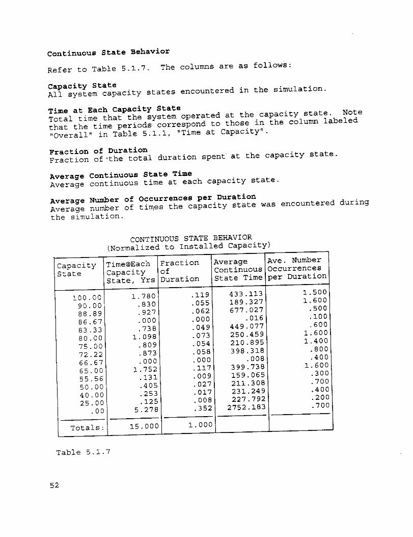
Continuous State Behavior

Refer to Table 5.1.7. The columns are as follows:

Capacity StateAll system capacity states encountered in the simulation.

Time at Each Capacity State

Total time that the system operated at the capacity state. Note

that the time periods correspond to those in the column labeled

,,Overall" in Table 5.1.1, "Time at Capacity"•

Fraction of Duration

Fraction of'the total duration spent at the capacity state.

Average Continuous State Time

Average continuous time at each capacity state.

Average Number of Occurrences per Duration

Average number of times the capacity state was encountered during

the simulation.

Capacity

State

I00.00

90.00

88.89

86.67

83.33

80.00

75.O0

72.22

66.67

65.00

55.56

50.00

40.00

25.00

.00

Totals:

CONTINUOUS STATE BEHAVIOR

(Normalized to Installed Capacity)

Time@Each

Capacity

State, Yrs

1.780

.830

.927

.000

.738

1.098

.809

.873

.000

1.752

.131

.405

.253

.125

5.278

15.000

Fraction

of

Duration

.119

.055

.062

.000

•049

.073

.054

.058

.000

.117

.009

.027

.017

.008

.352

1.000

Average Ave. Number

Continuous Occurrences

State Time

433.113

189.327

677.027

.016

449.077

250.459

210.895

398.318

.008

399.738

159.065

211•308

231.249

227.792

2752.183

per Duration

1.500

1.600

.500

.i00

.600

1.600

1.400

.800

.400

1.600

.300

.700

.400

.200

.700

Table 5.1.7

52

Print

Use this feature to generate batch printouts of one or more of

the Performance Results in Section 5.1. The window on Figure

5.1.8 will appear when Print is selected. In each field, enter

the number of copies (up to 9) you want of each table.

[i] Time at each Capacity.

[I] Capacity State Availability.

[0] Cumulative Availability.

[0] Equivalent Availability.

[0] System Capacity& Overall Availability.

[0] Reliability.

[0] Capacity State Behavior.

Figure 5.1.8

53

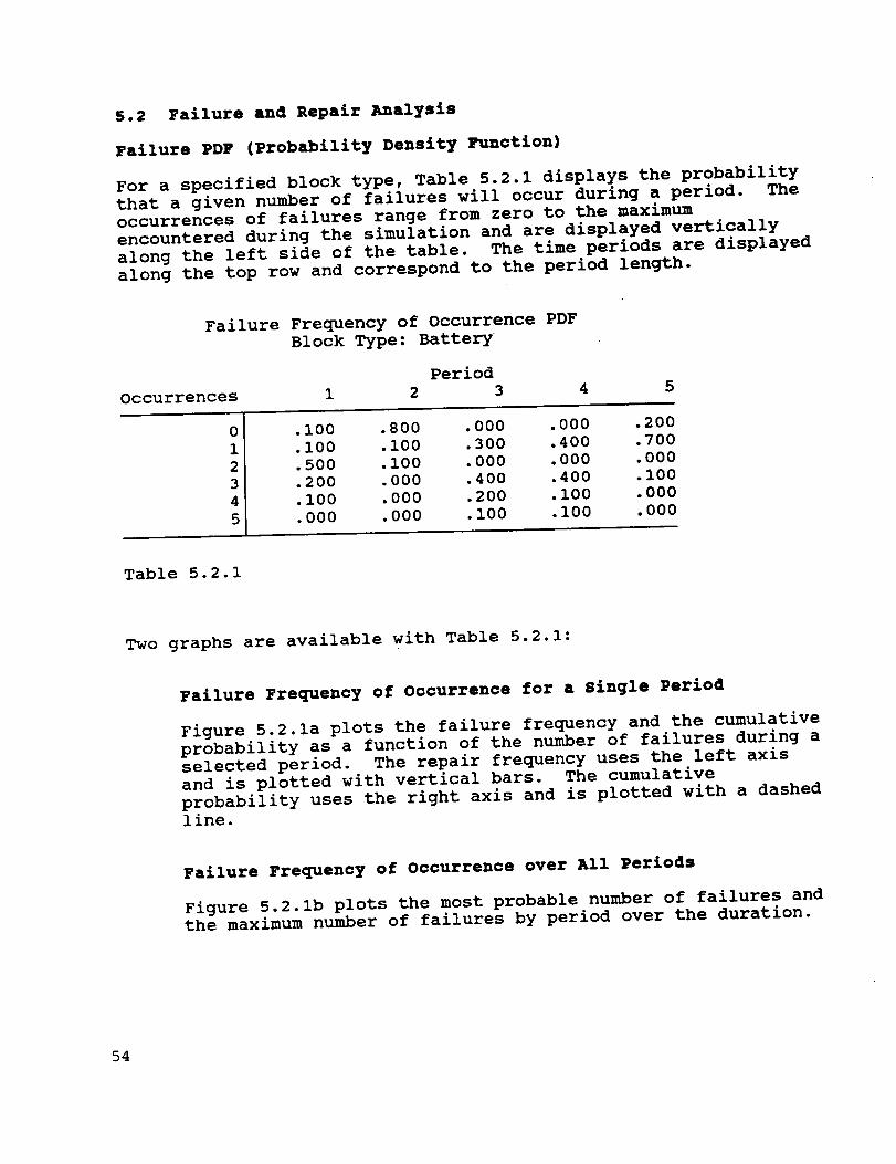
5.2 Failure and Repair Analysis

Failure PDF (Probability Density Function}

For a specified block type, Table 5.2.1 displays the probability

that a given number of failures will occur during a period. Theoccurrences of failures range from zero to the maximum

encountered during the simulation and are displayed vertically

along the left side of the table. The time periods are displayed

along the top row and correspond to the period length.

Failure Frequency of Occurrence PDF

Block Type: Battery

Occurrences

Period

1 2 3 4 5

0

1

2

3

4

5

.i00 .800 .000 .000 .200

.100 .i00 .300 .400 .700

.500 .i00 .000 .000 .000

.200 .000 .400 .400 .i00

.I00 .000 .200 .i00 .000

.000 .000 .I00 .I00 .000

Table 5.2.1

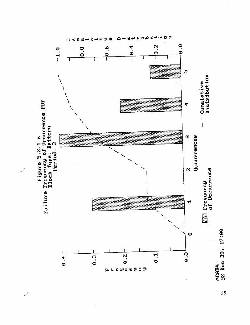
Two graphs are available with Table 5.2.1:

Failure Frequency of Occurrence for a Single Period

Figure 5.2.1a plots the failure frequency and the cumulative

probability as a function of the number of failures during aselected period. The repair frequency uses the left axis

and is plotted with vertical bars. The cumulative

probability uses the right axis and is plotted with a dashed

line.

Failure Frequency of Occurrence over All Periods

Figure 5.2.1b plots the most probable number of failures andthe maximum number of failures by period over the duration.

54

.w.l

! •

i I i i I i I i I I

\

\

\

U= \

0

\

UU

0li) ,,_

_.,_

I

I

u

U_

_U_U_0

_0

ii

U

_N

_) 55

r,_

c_

,,No t_

• C_ *i

I,_=o

,,,Ill

IT,,

ti !iii!!iii iiiii

..... iI

q_

N

i .......... .'.'° ...........

I ! _ I , I , I _ t

I

°l,,I

ID

iliI

>¢

T-

a_III

C_T-

q-i

C,I

l_l=l<Z:

56

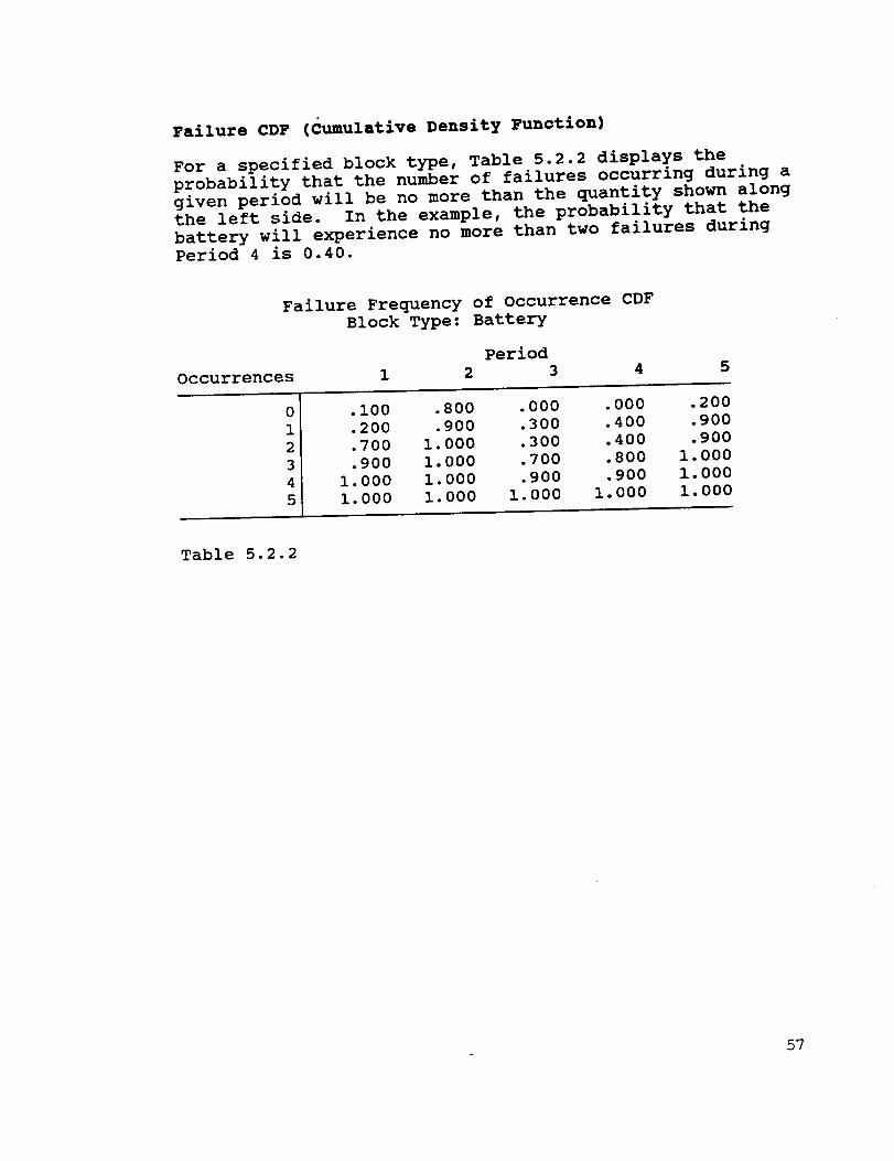
Failure CDF (Cumulative Density Function)

For a specified block type, Table 5.2.2 displays the

probability that the number of failures occurring during a

given period will be no more than the quantity shown alongthe left side. In the example, the probability that the

battery will experience no more than two failures during

Period 4 is 0.40.

Failure Frequency of Occurrence CDF

Block Type: Battery

Occurrences

Period

1 2 3 4 5

0

1

2

3

4

5

.i00 .800 .000 .000 .200

.200 .900 .300 .400 .900

.700 1.000 .300 .400 .900

.900 1.000 .700 .800 1.000

1.000 1.000 .900 .900 1.000

1.000 1.000 1.000 1.000 1.000

Table 5.2.2

57

Early, Random, and Wearout Failures by Period

For a selected block type, Table 5.2.3 displays the

quantities of early failures, random failures, and wearoutfailures that occurred during each time period. A bar chart

is available for this table and is shown on Figure 5.2.3.

Note that these results will not be available if you have

specified that you did not want to track the failure types

(page 16).

Early, Random, & Wearout Failures by PeriodBlock Type: Battery

Failures

Period

1 2 3 4 5 Overall

Early 1.900 .000 .400 i. I00 .i00 3.500Random .200 .300 .300 .i00 .i00 1.000

Wearout .000 .000 2.100 1.300 .800 4.200

Total

Table 5.2.3

2. i00 .300 2.800 2.500 1.000 8.700

58

0

iL i

tt_

!

_I

,, ,.. . "..,.,rr.: .x-_.._. .r_......;.::{...-.r-....{._÷-..Z. i

,-2 . ".'--..',_4z'z'.gz_?d_:_

I

i

_::_:ii::::':;::;::::'::;':::':"::::':::";;::f'::;:":::;':::;'::::i""I":::2"_":':--_'2--;-'_-_;-''-±'_--':-T"---:"-+i:÷:'::+:'z:::_

Z:-".-:-'-": ,'Z.-F"-':."> :':'-"-,:-"..(-". ".-':.:.'")":":":Z."-" "'..'.---'..-._Z;-'-Z--_ 4-D -:-.L"_L':"'-'::,-," - -'."- ":-'..-,:-".E-_'-. _

:Z!":_.!:': ! :i::i! :i! ii .'::_i:ii.i:_:: i::i'[-ii::i:ii'_!_:i:i::'[ I _.'-_:-_!',._-_D--.'_:_--." _:_ii_ _,_j_::::::::::::::::::::::::::::::::::::::::::::::::::::::::::::::::..;;2-:H:--:_2:_.:Z:::2r..-.-::,:x..:_:...::;Z:--_-gziz_.zz.::_

I.................................... 1

"........ "- " • "$"F"_:.-:=':.'_-_.-.'a_'-'E.-2--7: :-'..'.'.-T. ff.:,:-:.:-..,_..t....-..... "...--.,.: ÷:-'F ".'-.':-':""-'--.".'.-":.-" v...-'..'.",,

"".'." Z-'Z, " ' .; .u. :,.. :...Z... -._....- .:._....z.._....-.._;':t.;Z_:: ....... ...-:;.'.':.'.".'._--'.'--Z:.-Z_};{-'D-C_:._r_'r:=_:4

.,':.'.-:.'..:." " " •. "t_:_r_--_::_:_:-..._T.:_....:_-_._-._:-._.--_=_.-_.:.-;_-_:.T._:_-.:_:..:_._._-_-_-_--._..-..._..._:CZ_ Z-:_

-'-.[..'.-:.'"--_ . - • [`:.Z.........v_-:...-_:._:....D...::....::_.._._-..:.:_--.......F._....._....._._......_:_.._::_._L._.-.Z..:_:._..-._...._.._...-..._.-.._.._

iIi

I

t_

i.o.._ •Io" i

! • • o _

::::::::::::::::::::::::::::::::::::::::::::::::::::::::i;iF.:i:_:i:-!;!:i;::::.i:i::::i::i::!:i::-i:!.:::i:::-i:i;::i::!:_:!:!il" i;::-'::,::-:.-:':.-;::::::::::::::::::::::::::::::::::::::::::::::::::::::. . .

,., ,-, .-!,,-:,:--:--..----..----':.-..';<.',-: -;--."-...':.-:.-::-..:...:.-:-:.-.'-:..':->.':-'.--:.:.-_- I"" "" "" "" ".........""_'.:..""""" :,-:,.'::';,::.-:,I.::-; "i

_ .- .,.- ...-_ o_, _ ..., .v _ - o. ....

,..:....:....:,,:.:.::. :i_,::-:-2::_2.:_2:9_.-::.::-_:.:;:::-_.'.t,-,-_,::,2.'.-_:;-_ ','.".-.-4:--..'.-..-'-...'.--.-:.-".-:.--'..-..,_- - ._

:,';.',-'X:--;,'.-::,::::::-::_._:,::..'.::.I::¢_:::.:::::.:-¢:::-:::::-:::._:_'..' .ii-'.--',"-Z.<.".-..".-"."."-"."-'.'.".'.-':4-':.-':-".-.'.4.-...'.<,':,-"

.,,_©

_ ,,,,,,,,_o_

L

59

Repair PDF (Probability Density Function)

For a selected block type, Table 5.2.4 displays the

probability that a given number of repairs during a given

period will be no more than the quantity shown along the

left side.

Replacement

Occurrences

0

1

2

3

Frequency of Occurrence PDF

Block Type: Battery

Period

1 2 3 45

.500 1.000 .000 .000 .900

.500 .000 .i00 .000 .000

.000 .000 .400 .i00 .i00

.000 .000 .500 .900 .000

Table 5.2.4

Two graphs are available with Table 5.2.4:

Repair Frequency of Occurrence for a Single Period

Figure 5.2.4a plots the repair frequency and the cumulative

probability as a function of the number of repairs duringthe selected period. The repair frequency uses the left

axis and is plotted with vertical bars. The cumulative

probability uses the right axis and is plotted with a dashed

line.

Repair Frequency of Occurrence over All Periods

Figure 5.2.4b plots the most probable number of repairs andthe maximum number of repairs by period.

6O

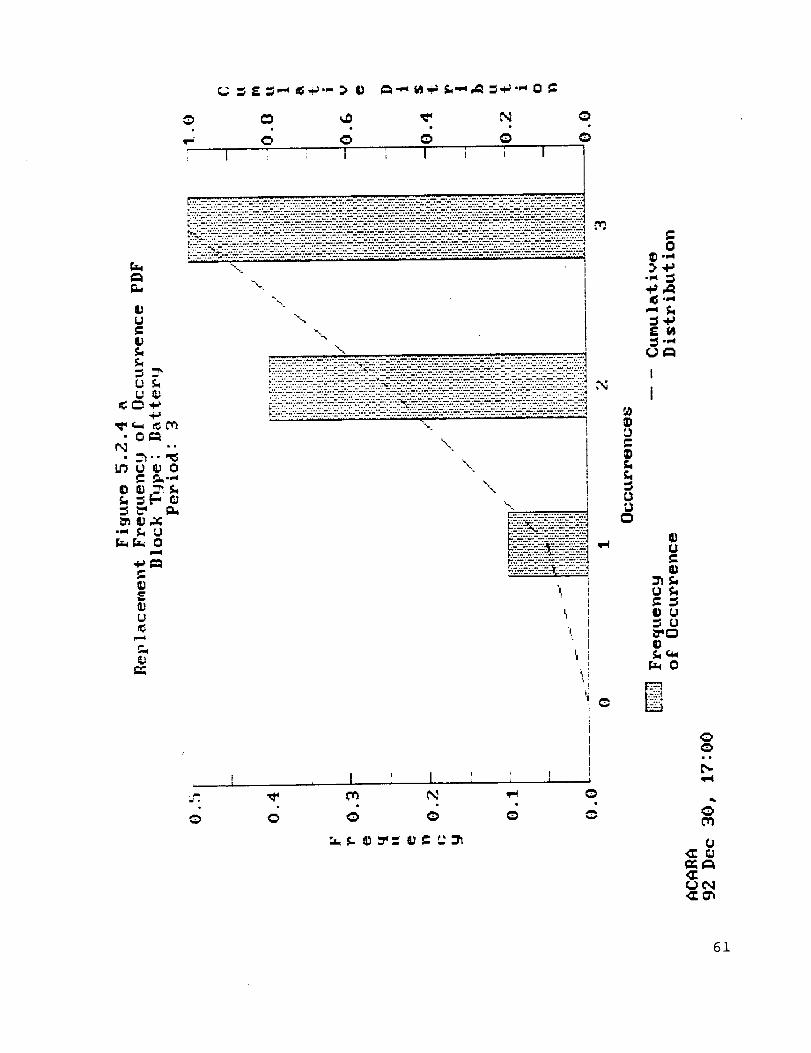
r.i

; I ; i I

i

"-....

t"%.,.

"_...

"!(

II

|I ' I i I

r.j

¢=o

:,..i-,,

I

I

_J

(J

6Z

tata

• ............. I

I..i-i- -_o-i- -. -:-i-it ............. "

!li i i I ! ; I f I I I I I 'J I ! I , I i t i

¢_, I,i',1

E

E-ml

T-

[;

B

I_1=1

ON

62

Criticality

Table 5.2.5 displays the mean reduction of system capacity (%)

caused by a failure of each of the block types in the system.

CRITICALITY BY BLOCK TYPE

Block Type Name

Turbine

Generator

Diode

Battery

Outlet

Mean Effect

of Failure

on Capacity

4.00

24.56

.00

10.59

16.50

Table 5.2.5

63

Accumulated Early, Random, and Wearout Failures

Table 5.2.6 displays the mean number of occurrences of early,

random, and wearout failures for each block type.

Note that these results will not be available if you have

specified that you did not want to track the failure types (page

16).

Accumulated Early, Random, and Wearout Failures

Block Type Early Random Wearout Total

Turbine

Generator

Diode

BatteryOutlet

.000

.000

2.000

3.500

.000

.300

.200

1.600

1.000

.400

.400

.200

.000

4.200

.i00

.700

.400

3.600

8.700

.500

Table 5.2.6

64

Individual Block Failure Results for a Selected Block Type.

Refer to Table 5.2.7. The columns are as follows:

Block Number

Individual block numbers associated with the selected type.

These numbers were defined by the Block Numbers Input Table.

Mean Occurrences of Failure

Number of failures for each block. This is the number of

failures experienced by each block divided by the number ofiterations.

Down Time

Down time for that block, expressed in days.

% of Duration, Down

Percent of the duration that the block was unavailable.

Delay Time

Delay before a spare can be supplied at the next spares

replenishment action. Subtracting the Delay Time from the

Down time yields the active repair time.

Individual Block Failure Results

Block Name: Battery

Block

Number

6

7

8

9

i0

Ii

Total :

Mean Occur-

rences of

Failures

2.00

1.60

1.50

1.20

1.50

.90

8.70

Down Time

Days

1853.64

1362.64

1710.17

1455.63

2035.55

886.63

9304.26

% of

Durat ion

Down

33.86

24.89

31.24

26.59

37.18

16.19

169.94

Delay Time

Days

1853.58

1362.59

1710.12

1455.59

2035.51

886.60

9304.00

Table 5.2.7

65

Failure and Repair Results by Block Type

Refer to Table 5.2.8. The columns are as follows:

Block Name

Block type names as defined in the Names

Input Table.

and Properties

Block Quantity

Quantity of blocks of each type.

FailuresNumber of total failures divided by the number of

simulations.

Failures/YearNumber of failures divided by the duration.

Repair timeActive repair time (days) for each block type.

Repair Time, %TotalPercentage of total repair time associated with each

type.

Down time, %TotalTime the blocks of each type were not available divided

by the total down time.

Delay time, %Total

Delay time for each type divided by the total delaytime.

66

Failure, Repair, Down Time & Delay Time by Block Type.

Block

Type

Turbine

Generator

Diode

Battery

Outlet

Total:

Quan-

tity

2

1

3

6

1

13

Fail-

ures

.70

.40

3.60

8.70

.50

13.90

Fail-

ures

/Year

RepairTime

Days

.O5

.03

.24

.58

.03

.93

.00

.00

.04

.26

.05

.35

RepairTime

hrs/yr

.00

.00

.07

.42

.07

.56

RepairTime

%Total

.00

.00

12.05

74.63

13.32

I00.00

Down

!Time

%Total

12.75

Ii. 74

1.69

73.21

.61

i00.00

Delay

Time

%Total

12.75

11.74

1.69

73.21

.61

i00.00

Table 5.2.8

67

5.3. Lifecycle Cost (LCC)

This section deals with the costs of hardware production,

transportation, and maintenance. The names of the three

maintenance operations, i.e., "Crew", ,,Equipment", and ,,Robotics"

are arbitrary, and can be changed appropriately. (See page 35.)

Hardware Cost

Tables 5.3.1 a and b show the mean hardware cost. In Table

5.3.1a and Figures 5.3.1a and c, the cost of hardware accumulates

whenever hardware is fabricated. Since these costs result

directly from the production quantities input, they will be

unrealistically high if the simulation assumes unconstrained

production quantities. In this case it is better to show thehardware cost accumulating when hardware is installed, or when

failed hardware is replaced, as in Table 5.3.1b and Figures

5.3.1b and d. You can select either approach from the Lifecycle

Cost Results Menu.

Mean Hardware Cost, $kPeriod

1 2 3 4 5 Overall

Turbine

Generator

Diode

Battery

Outlet

Sums

Table 5.3.1a

246.000 .000 .000 .000 .000 246.000

24.600 .000 .000 .000 .000 24.600

.180 .000 .000 .000 .000" .180

71.400 .000 71.400 .000 .000 142.800

.255 .000 .000 .000 .000 .255

342.435 .000 71.400 .000 .000 413.83b

Mean Hardware Cost, Sk

1

Period

2 3 4 5 Overall

Turbine

Generator

Diode

Battery

Outlet

Sums

Table 5.3.1b

164.000

12.300

.085

71.400

.085

.000 .000 .000 .000 164.000

.000 .000 .000 .000 12.300

.009 .005 .009 .011 .119

.000 33.320 35.700 2.380 142.800

.008 .017 .008 .000 .119

247.870 .017 33.342 35.717 2.391 319.338

68

_g

t,,i f,,i_1'II

g',l"

l 1

_2Z.2:::'27"_-T-2'-/-:.z2 0

:e_.-e-ez_.-'--.e'ze I'_

"2-.---.2.-2: _27 :-::.....................

E-:-.Z::':-__'" ................ :_-- ........ ,:."2:_:-" :'-:.-:

___._ _._.;.._._--:_-_::.-:-*-_:__ _.................................

__ ..... "-- ............... -::::7 ......._-t. -:::_Z-." :_-:_-:-__÷-+-+: ...... -...... ........ '22.--_-_7--2:

I _ I , I i

I,}d:G)

I.._ IN!

69

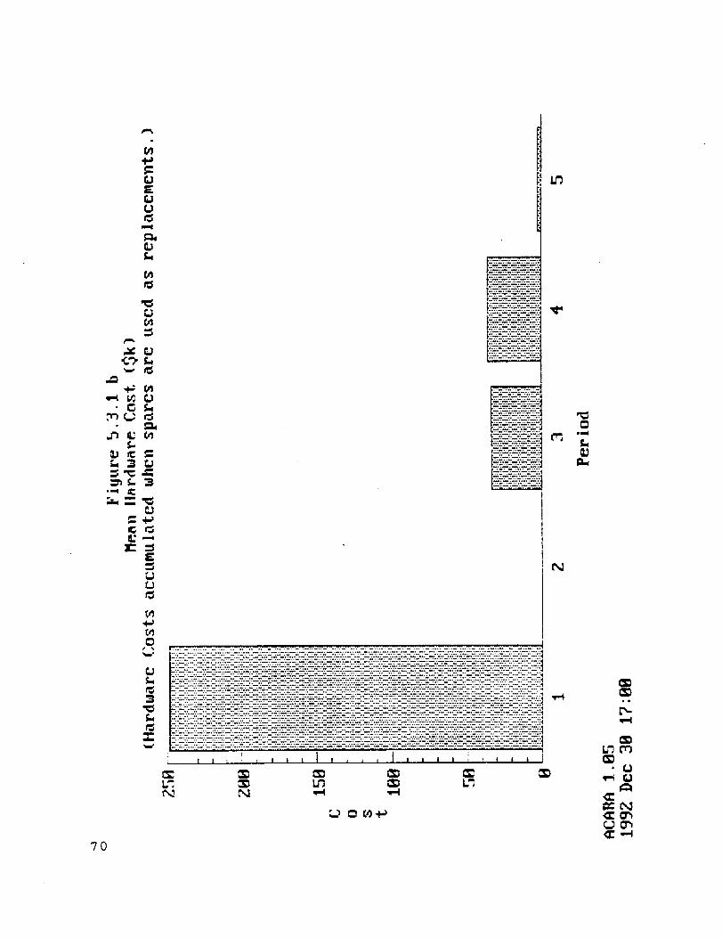
E

c

E

,_÷_..-.-÷-.-÷..-..:

_-:-_--.'-_-.'--_+z-"

'2"?"2:';.._-'7"2:;_'.'.: f_

b_

Ill:,liilliiiiliil!_llll

7O

,iiI

b_,_

• 0

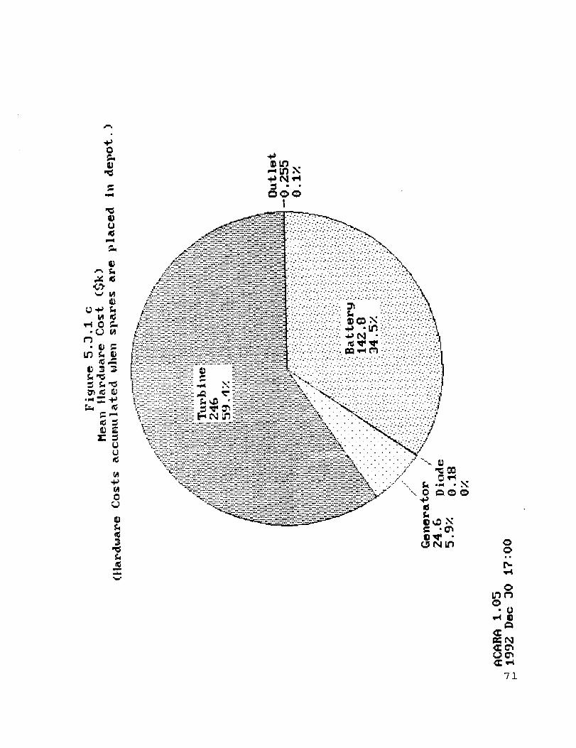
O

't#

U

,-, I/1

U

0

m

•, ._-_..ze;_ez_ez:-e"--e._-ze_;Z_"f.'.-'.'.:-'.:-'. :." .'4.7-.'.-.'....._ ::::::.::-::.:-:c:;:-:;i--f:;_-_, t-z::_-::::-_--; ......;....-....:.....,.:;.:;.,../:._;.:-;.:-..:.._

, .._-- :::::::::::::::::::::::::::::::::::::::::::::::::::i:::._!:::::_,.-.:-:-_!-_ii_-i:_-__=;i. :_.;:::.::::._::.:.::;.:::_::::.::::.:_::.::::_::.::;.:::_:::_:::::.::_::_::_.`

iiiii:/:i!:: i i i:iiii iiii:i i:i:i : i::::i:: !:!iiiiiiiii !i:i!!i _-!i-i_E.:i _[-;}.:-.:,.}::-;}:: r_ ×""i;:-_?{::i:":(;

_-i_.;.:::-::-:.z::-z._:_2:_;_-_2.:2?z.?:_::..-e?..:+::p_......_.X_..:..}.._./._....._ _ • ":'..-.'.--.-.'.;.....-....::&

. :----±:cS,_:.::;-:"'.z-::_;-::_-_]_-i±Z:2-_---g.2" ..':-'.'-;v ..-}..-:.-:..._ C,_ • ..-':-/-:"., "]-:--.".-."..i:-:.±:.z:.-_:?;-.:-z-:.zi-::.-:..-:._-:_-_±-_.:.T.±-;2=:2T_-.:-_-.-:-:-.=::±?272it..-..:-/..;-:-;..-;.:-;-_';_ _1__1_ :..:.:..'.::'-:.-...-..: r..;

'_ii:..:-_:._?--:-_-- :;-::;.::;-::;-:.;-:-?-;-::.._.--....-r2--,::-:-::-:-:::-;::-;:<:::-:_-:--:--:-_!-:.-i!;-_ii-!_-_--%............g_Y.-i-_,.:.-:."'.--:.-:-:-:-:-:-:-:--:.::-.:--:-:..-:-i:4:4:4:.-:;i:--:.-..

:::-:>-=:..-;.>:.--":+-.'<.z-:-" _ +-.-:-.T.ei.:e't_.z-_z_:._,'-:.k -'- .-':.-; :.- ".- . :." :.'. % ;.'. :......'. .-.'. .'..-..--.."t.-.---v.;y-.----.':...... "..-D-:-..-- ,_.-'._----r--.-.'+._._-l-..w.÷z-:+:-z_'_ ,,,.4. "..--.--.--.'--'--'--'--". :--- :- "- "-"- :'.-.

!i:!i-;!i_::_::Y:_!:--:fl-i!:;::_!i_, _'_!i_i_!--__"_-":_.;:"_:i:::::::::::::::::::::::::::!:::::::::i:.'-:::::::::!:::::::i:;::',-:-::-:"-:.-..:.t::-f:!:-:::-_ _.i ' e:'--:--_±:;::Zg±T-._.=::::Z-:::::-c..-". "':'4".L...-'. ,-."--'..:..-":.-'...'. ..":'.".':".'._;:-:::;;-::;z-.+:.:-:-z-:-::-2:;-._ _ _'_z-:::z-_:-_:.:-±--:.-.i.+.g±.?.:_. - -_"_... ,-.-. :.....::-: -.'.-X.-'.-..-;'."-__/:k:::<:--""-:-::+:"..-.,,'-_ _ _ _-_=.....................................................:.-.-+-_.-.:+_,_" ,.. '-.v.:-....:-_:--.-;.-;vi--';"

_'_'.".v.---". -. --r -.-_.......... .Z--F'r'-I-._'_._'.-.._'..-.'.'.._::'_-:'r-_:÷:.Z÷_-F:_÷_._ ...... ", -': -'t ": "': " :'.y

,;---::--.z-ez÷£_-+--:_2T:.±:_-_N=-±_2÷:e:+_-.+:.z._zez_?-T2z.2g2...".".".".;.... _ _-_

_--i::.:Z::-.-±g-:::;-:-±:--:'z--:-::_-:_-+272-2---2- :_-:?--':-_"

i_ ,_l,_ •0

O

O

"71

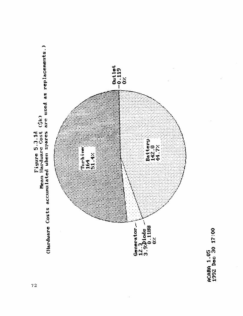
51

ILl

it,1U

f...,¢1f,,,

f,.,

I,.=,=t m "'_

_,=,,

n_

o_J

tD

n_3

z

?2

i

_DN •

00ee

t-

o

_N

Transportation Costs

Table 5.3.2 displays the mean transportation cost for each block

by period. This is the cost to deliver hardware for installation

and resupply. It is assumed that the transportation cost for a

given block type is directly proportional to the delivered mass.

Figures 5.3.2 a and b show these costs in graphical form.

Mean Transportation Cost, $kPeriod

1 2 3 4 5 Overall

Turbine

Generator

Diode

Battery

Outlet

Sums

Table 5.3.2

.774 .000 .000 .000 .000 .774

.468 .000 .000 .000 .000 .468

.002 .000 .000 .000 .000 .002

.956 .000 .446 .478 .032 1.912

.005 .001 .001 .001 .000 .007

2.205 .001 .447 .479.032 3.163

73

74

X

N_"0

E

d_±-:

N

_--L-::::2_ -2Z:_-:_ ............................

! I i I I I I I i i i I I I I I i i I I S] I | I

WJ • • • • •

i:1

I,)

m.

,{3

-(a,,=I (}

<_ .,..4

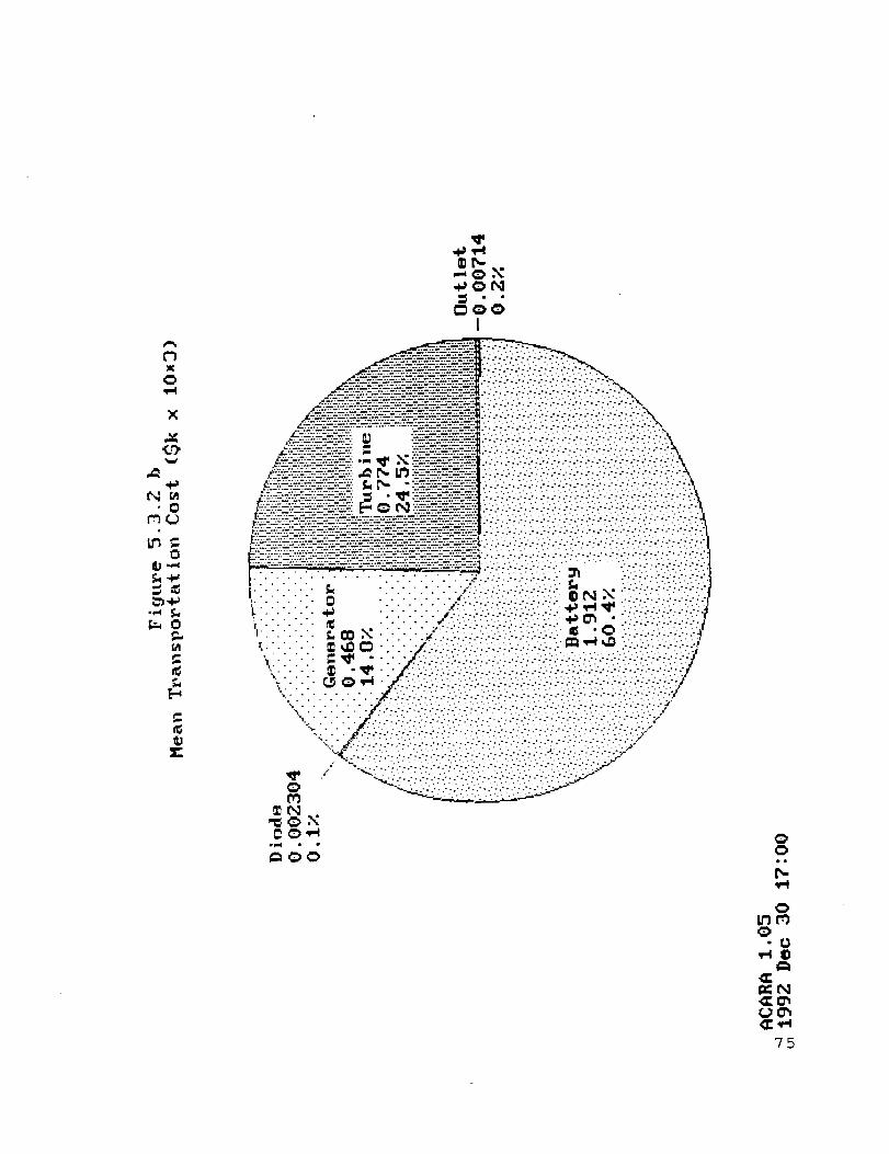
t_

0

×

t'4_'0

0

T-

00e_

0

-0

_N

75

Crew Costs

Table 5.3.3 displays the mean cost for maintenance action #i

(Crew) for each block. This is the cost to replace the failed

blocks during each period. Figures 5.3.3 a and b show these

costs in graphical form.

Mean Crew Cost ($k x 10"3)

Period

1 2 3 4 5 Overall

Turbine

Generator

Diode

Battery

Outlet

2.160 .000 .000 .000 .000 2.160

.416 .000 .000 .000 .000 .416

.113 .012 .007 .012 .014 .158

.528 .000 .246 .264 .018 1.056

.184 .018 .037 .018 .000 .258

Sums

Table 5.3.3

3.401 .030 .290 .294 .032 4.048

76

rd

"0

[,_¢1

@

_N

t,,iEl

I

ii

ON_:_

?'7

I

'78

i{

' 'f.3"

.,.i il,1

,r

r-

<l:_N

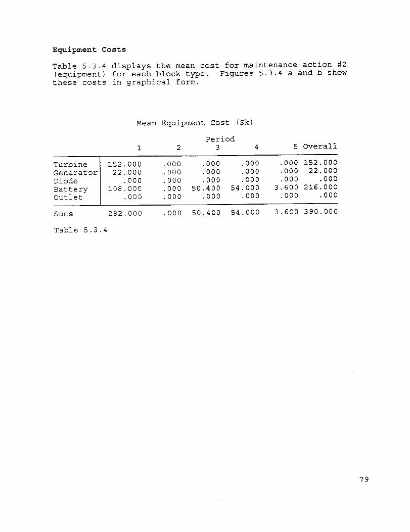
Equipment Costs

Table 5.3.4 displays the mean cost for maintenance action #2

(equipment) for each block type. Figures 5.3.4 a and b show

these costs in graphical form.

Mean Equipment Cost ($k)

Period

1 2 3 4 5 Overall

Turbine

Generator

Diode

BatteryOutlet

152.000 .000 .000 .000

22.000 .000 .000 .000

.000 .000 .000 .000

108.000 .000 50.400 54.000

.000 .000 .000 .000

.000 152.000

.000 22.000

.000 .000

3.600 216.000

.000 .000

Sums 282.000

Table 5.3.4

.000 50.400 54.000 3.600 390.000

79

0

"d"

_f,,_,,.,p.O

N

I

..... . .." '..."..."...-..."...-.-.".-".-.---:"*v*Z..-Z":'Z': .............. .'"-."'..'".." --'" ""..'"..'.':-.'"-.- "-,""-'_"'-'-"'"'7" L .... Z

.................. _ .. "". .... ,": .": ,"'-'._'..'"..'"..".-" -.".'-":-.-'-r"-'-"_'_-_'_-.'.: "-"-"'-F' :t"..." -." ..-"--"-."..."--, .-_Z_.:_rr:_:-r_:._w_._.r;.-_:_::_._:_`_-_;.-_-._;_Z_-.._-.. ..... ...-.......,..._..'_

"...",.,".. ,"-.." "--."-.'." ".. """.-"'-"Z" .}':-.'Z.:-Z:-'Z-Z-".'._..'." ., v_v...-,-.-..": ................. _-. _--_-. _-r.:.:.'_-;_t-_. ,.ZZ':-ZF.-Z'.":'[:Z-rZ'F -"L -" ".}4

i i , I ! , 1 ,u-,4

,$

80

.,!o

.¢,'y

r_

t"l

_r,,_

-::i-:-:::_::_:{-{-_ ..>...-....-..:....'....._..:...:::.': :: -_..,,,

_--:.:v.:.-/.-/.-:.:-...:...-:.::.:.:.--::..-:-.-,

,5:?!::::2.7_2z÷z...-.:+-+-:. +_±__._].___:-__i-._-._--'....-.'-..-:.....>..-.:.....:.:..:...-...-.._. .. -. -. -. -... -. -.-.-.-.-...-..--.-,

._- -:.-7-}:-}..:-:-7.:..'}}}-I-..;:.-:7-7.77.F{7.',,t.-._."-_ - ............ .'"., ,...-......,...."............-....-......,.......-...%

_'(-:+::-:"_':'D"::':" "-" '.'Z'_ _-E'+:Z+ -_+'-:' ................. :.. :....:.,.:-.:.. :.-....-....-.....?_...t..'..}....._.....:.......:._

r-_-..-.-:..- ."--':. :- :- "- "- "- "- .'- .- .• . • . " .- .".. ". ., .

/- -r.._-.._-.-_.-r.':.'r_--_.-:_.'r._-._'_.......................... _ '.'-.: "." .." ".: '..'..."..'.-.'-.'.-.'.-.'.-.'.-.'.-.'.-,'.'-."-." -_

_-S:.:-:_::-:->-:-::............................... }.-?.-:..?..7.-7.-.v:...-:--.-::-.v'.-Z..-}..7k:i-t/-}}-_,_::-:':-::2::::--'-.-.-'-::2::?-_i-':_ --"'T-'-::-_:--.±::::±:Ve±:-'-2'_!."--"-.'-.'...:..:"."-'.'".'.'..'-':.'-'." :.'">".'".':-'_',-:-..-".-----,':.-,--,,--,-_ ±::_±-_.':-:_--_: ....._._}.._}...}._..}...._..::.:__...._.......vv___.._........:.:_....::.h.:__:.

::::::::::::::::::::::::::::::::::::"_ .t-_tE_--!?-:-:-:T:...v:..7:-7:-7:-k.-7..7..Z.v..}7.:vl-vT.}}_i:.}k.-i--ii:.tl-}.:::::::::::::::::::::::::::::::_ X "_:_:?--:-z_?-_-_....->.-..:>:..:.-.'.-:.-..-:.}:'..:.::'.-:..:..-:.-:-::.':.-:.::..":::::::::::::::::::::::::::::::::_ _ • " --.f:--_:+?2?±.--:::--..?2_:..:.-_.._.._._.._....._...:...:_:_..._.._._..._..._..._:._:._:.......:_..._....:::::::::::::::::::::::::::::::: ,, I,_ _I_'_+:-z::--...2?2-:±-T.-_-'-.".-X..'......'>::'.."l_ -':":":-'"""":-:".

!ti:-::-::::::-:-:-'.-;_-:::;-:-::-_ ',_ _ ---_---_---::..-::-":-:.-:.'.-.v}'.-}'.- _ .'_ .):'.).v:..:.-:.-:.-:}::

_::_7_._:r_.Z_._.:..x_.:._.....-.-_...-÷-.._+._;+-_+_Z+_z_:.7:_:_-_¥ "" _' -""-'."-': .';-" -': "':'" 1t" _ ". :'." :'" :." :." "." :." ".'- t

I_:::::::::::::::-::--':--:"--::-:-:.z<-:::%:-_._£_:£'£-":':':::2_-_2_-.'.-.'.-:.--'.'..:'>.:.'-'. ",_ ',,,9 " ":"" :" : ".':'."'.".'.'.'.':ii:::::::::::::"--":.-i_;:i:::-:-Z-_::-:?':-::-+'_-"+:-"-':f_2?2;:. ):>".--.-:'.-:."-'--:..'.'-." _ _ It') -'--':.':":""-'" ".:'1'i:::-::::::--_:-::-::-:E_E_7(--_:.--.]_F"..p...v::-::-7.-.-7..k:.i.:-m _ _ -I:U{:I-Zi:}"2-:

_..i:-Z.Z--:---'+Z÷Z---:.L--:÷::÷:- ._-Z7...-Z.r_Z-_.:._÷.-..:.F£._÷ 7 . . _.-.'...-. :...'.....-..-: .-: .-: .-:..-: .- ,.-:. t-: .-, ..-: -'....-: .:": i.":-[: _ _

'i:,:-::::t:::z::-:-:::;--:q-i:_-_"--t.---,e. •. t: :.' :., :.[ :.- . i- . :-. ::. --..v...}.:... 7..---."-.-"-..".-{..(..-..-"ih-:::::::±:;::z_:7.x-±_z#.:::_-:_.:%-:.-..2::-_,.-. ;_-.....:........-..::._:.....:.--.:....-...:... .-.......-.:.. :-.....-.....-....-......./

'::::%:::-::E.P:F-F_E----_" " ' ' /." :.{vT. 4v{:-(".i'-.7.%%:...7,.....:-:..?.-}.".:i./,i::Z._..,(.- Z.r:.Z.:..-.,;i._--9-,_e_._. . . •. - . . ,.....-:... :.- .'., -... :.- :... ,'.-. ::...'......'....',...'..'..'.......-........./"-.@__-_.@;f::: :_'_:..._:_..::.:;:..:.:_.._::.:_.::_.:;_.:{:.:;_..:._..:..:._..:._:.;.:._:.:.f:.:_/

__'2":'±_±?::-_-' ... $-:"-:"-.-.:-:'..'.'.-.'--'.-.:-'.-X-.'.:--";--.-.;-.'.--.--'--:.-:'.-:_'_z:.-:-÷z:..:'". . . ...... ."-'.....-.-:-.-"- .: .:-.:-..-.---.-.-.>.-.-.'--.',_,"

",_.':'_.' ....... _-'"-"- _'- :- :- .'" "" :" . " ".. " • ".. t . ". " -...-.. '.

_- . - . -- -i- :-7{-:-_-: (-:{-:.}:(-:-i-.-[--::-(-:.:--{-S {-:.-:..J.,... .... _-:.-:...:..:._:.....-... :..:...:..:.. :.. ... ......- ..._,

"-- U: :. v:_.:v:v :.-:..::.::. :.:.: :.(u{:.:-_:.::

I ¢0

-0

_e4

81

Robotics Costs

Table 5.3.5 displays the mean cost for maintenance action #3

(robotics) for each block type. Figures 5.3.5 a and b show these

costs in graphical form.

Mean Robotics Cost ($k)

Period

1 2 3 4 5 Overall

Turbine

Generator

Diode

Battery

Outlet

24.000 .000 .000 .000

12.000 .000 .000 .000

.000 .000 .000 .000

72.000 .000 33.600 36.000

12.000 1.200 2.400 1.200

.000 24.000

.000 12.000

.000 .000

2.400 144.000

.000 16.800

Sums 120.000

Table 5.3.5

1.200 36.000 37.200 2.400 196.800

82

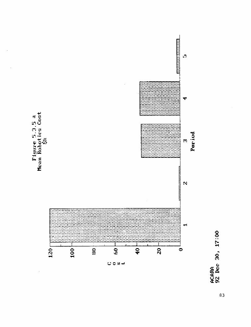
0

0

N

q-4

t_l _ _ _ _1_

0

83

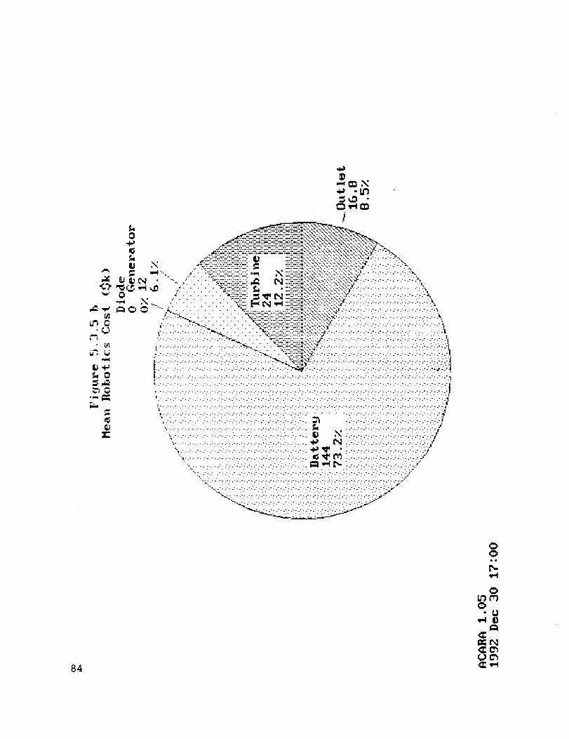
t..,_

r_

I1

•_ o I,i'1

•_--z=_'.':'-÷::":'-':'--z÷'_÷-÷--.':';'3;._':.'>,'.'._':.'.!S.':::::'.:,:_,:._.,dll __'-.:'.-_'£_':-'_:'-':.-::wZ ':':'_-.'::_':'E_::'::_,;'_:':.':X'_':': ::::'_::_::'::::-%_ .--_'-.,.

.._..-.7..=.:.:.:.:.E;._Z._.r-.:....: I,l ff-_.-+I:.*.N.-"-:-X£'-:.". .-.:-...----..-4- .'. :- -- _-.

ILl ,'_'. .-,:...-:I.;..--;._.-:;..:.-.._-.-.I.- _ .:.._.:._.:._..,.-:.,...-..-..:.:.:. .--,-.:,'._ ...... . i t_

_ ,,,,-1,,.CI /'" .... "'::z.--..z-:::z:I_ • -'7.'.':::_.M:::-:':5.::<:::::-:.::'.'::}': .':-'-. •.. -..---.. -..:'.,O "" " ." -" -" ." • _';":"_"-" "" _ ""'_ _':-"='':""":-":""_"''"'_ ........ .... " "'_

I_1 _. ,,_ ",_..- ........ _::.._-.._._._.-..._...Z.:;._.-_..:'..'.:.£_..:..:£..'_.'-.'...'..':.'..'..'..'..'-._-.'..'-."-',_...-'.L. " . " . . ' ." _'_'."...':'-.':'.."..:'_'-.':'...'.-.'-.X"-:'..>N'_'.._...... -." .... -." ............ ..' '_,,

....... • - -.. -""_.. ...... _-."-."---"---".--'.'_.".'-:':-"-_' • ........... ' .......... - - ..... .'1I ..... " • "_,,... .... _,:-:;.:.:.:._.:-..'.:..'-.:.:_:-.:-?.'.-:.,,, " " " ." " . " " " ".." ..'... t " • " • . • " 1

v • .'- .-..-..-- .-- ....-..-- .'_, .. -... -.',..-;÷-..-.:.-.-.:.7"-:..._,.::..:.::.,:./": -'" -'" .'" .'" -'" -'" .': -": .'" -'" -'" ." :" -.' ":": .:': -." - : I............. ..,,_. . -;,.:.--._.-_=-:-.,-..",-.-_ . ..... _ . . . . . . • . . . .- ........

J " " .... • " " ..... :_.- - . ":,:'.'-_'-E--_:+:'..:"_" " • ". " " ' " " ' " ...... ' "." ".- "-.'..."

; -" -"".'.'.'" -" .'"-"-':-': .'" -'."-'"-':-".":'_.-,,_ ".':-::3:-_:-:'.:.'_""-':-'."-'."-':-'"-'."-'"-'" ."-'."-'" .'" -'"-'"-'"-'" -'"-'._'.. ..... . .... . . ". . . • . .: ." _,:._:-.+-,]1 '.. . . .. • .... ".. ;. . - : o ... .... . '.- '.I ......... ':" "." ".''" : ." -'%.%"._,_ " " " " " .... "'.'""" "'.'" .'. '."" "-".'. ".'. '.: ".:

I-."-.", ."•.",."•."-."- , ..'- ."-."-."•."-."-."-."-."-."-._,_ ,"- ."-."-."-."•."..-- .".."•."-."•."-."-."-."-."-."- ."-_'- ."I

! '- "- --- - .:-".':-- ."-" ----::-4-.--.".-.-:.-:-.-:.-: -i

'.:::::::::::::::::::::::::::::::::::::::::::::::_::_::_::_::_:::::_::::::::::::::_:::::_::::::::::::_::;:::::_::::::}_::..:::_! " -'" """-'" -'" """-'" -"""" """-"""" -'' -""-'.'-'."-':-': -""-'" -'" -""-'" -''-" "-'" -""-'_ -':-°: -': ": -': -'1 -'" -"_-': -'"-"".-,iI

•,.............-............................................ ..... ..:....-......-........ ......-........_, ......-............-...........-..-.................. _ ..-......-:.-: .-:.-...: .-: .-..-:.-:.-..-,_

...:....:.......... _ N :::::::::::::::::::::::::::::::::::::,,..-.....-...........-..-..-..-..-.....-..-.....--.--._ N ..-.....-:...........:........./..::/•-_......-..-..... .: .......-........: .-...............,_ _ . .-..-..-..-..............-......_

--,...-..-..-:.-..-............................-.-..-.. _I ',_ _ ...........-:.-:..:..: .:.-..._."-,:.....-..-..-....:...-...:.::...:-..-.-.-..-..... 121t,_1 l'_ ..:..-:..:..::.-......:.....;"

.... ... . ... , . ." . . .., • .. ..,.....f

-..o...............................-. -..... -..-. -............o ....oo..°... • " . ' .. ". ..... - " • ," ." .. L - ".. .J

",.:j..........: ..: ..: ..: .-...-:.-:.....-..-:.-:...:......:..:....-: ..: .;:.'[;;,,,•,.:._ ..- .............: .., .-: ..: ............: .....................: ..: .'_..p

--.,:.L.....-...-...-...-:... ..: ..:......:.-:.............:.-:._.-_: .':-': .': .::-'" ."-':-.'.'_,;.z.*'"

84

C)

_.C_

_._

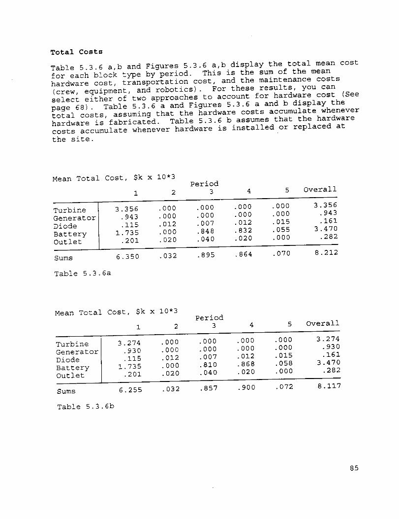
Total Costs

Table 5.3.6 a,b and Figures 5.3.6 a,b display the total mean cost

for each block type by period. This is the sum of the mean

hardware cost, transportation cost, and the maintenance costs

(crew, equipment, and robotics). For these results, you can

select either of two approaches to account for hardware cost (See

page 68). Table 5.3.6 a and Figures 5.3.6 a and b display thetotal costs, assuming that the hardware costs accumulate whenever

hardware is fabricated. Table 5.3.6 b assumes that the hardware

costs accumulate whenever hardware is installed or replaced at

the site.

Mean Total Cost, $k x 10"3Period

1 2 3 4 5 Overall

Turbine

Generator

Diode

Battery

Outlet

3.356 .000 .000 .000 .000 3.35b

.943 .000 .000 .000 .000 .943

.115 .012 .007 .012 .015 .161

1.735 .000 .848 .832 .055 3.470

.201 .020 .040 .020 .000 .282

Sums

Table 5.3.6a

6.350 .032 .895 .864 .070 8.212

Mean Total Cost, $k x 10"3

1 2

Period

3 5 Overall

Turbine

Generator

Diode

Battery

Outlet

3.274 .000 .000 .000 .000 3.274

.930 .000 .000 .000 .000 .930

.115 .012 .007 .012 .015 .161

1.735 .000 .810 .868 .058 3.470

.201 .020 .040 .020 .000 .282

Sums

Table 5.3.6b

6.255 .032 .857 .900 .072 8. ii/

85

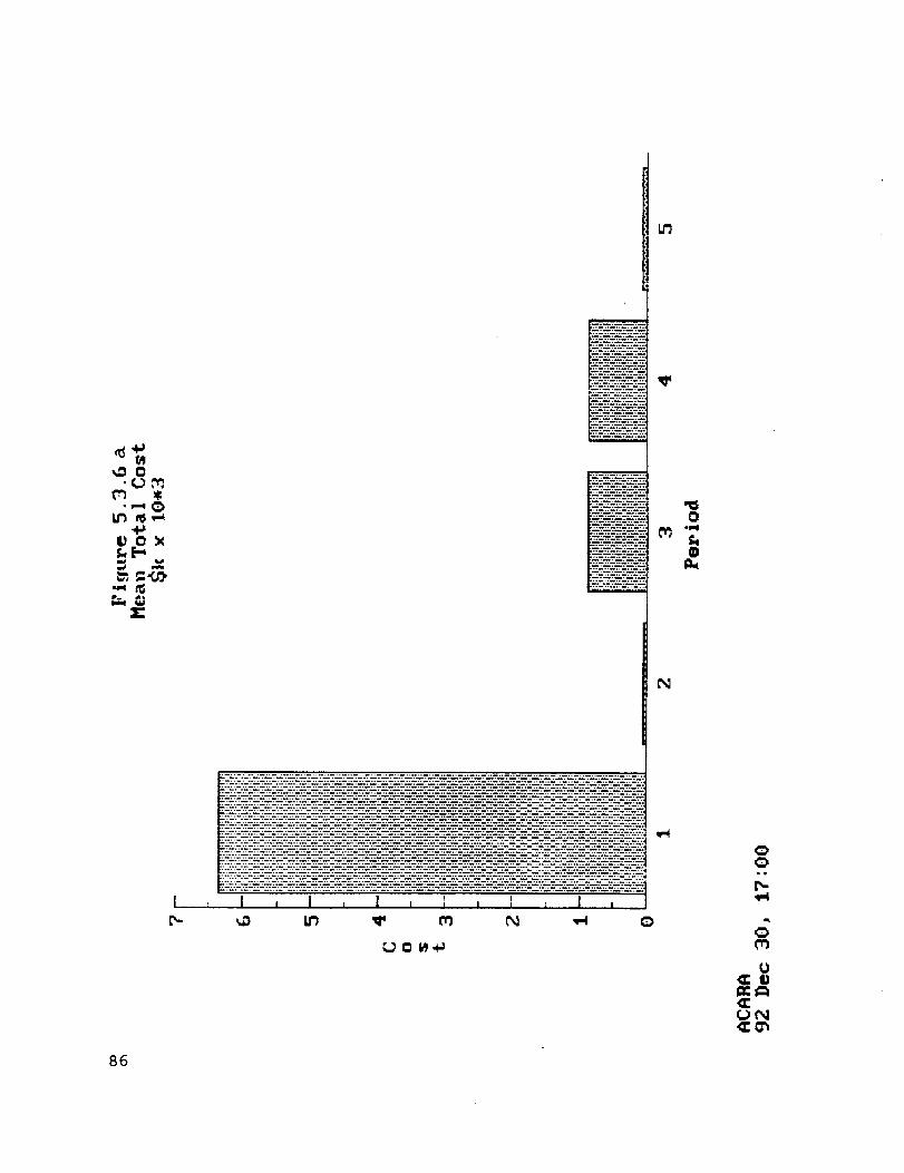
_0

T"

I

a

0

N

I , I _ ! , ; , I _ I ,r-

t_

u

ON

86

0l)

{aU

iml

X_

_(J3

[-,-

_UZ:U

mm

00

r-

0

-0

_N

87

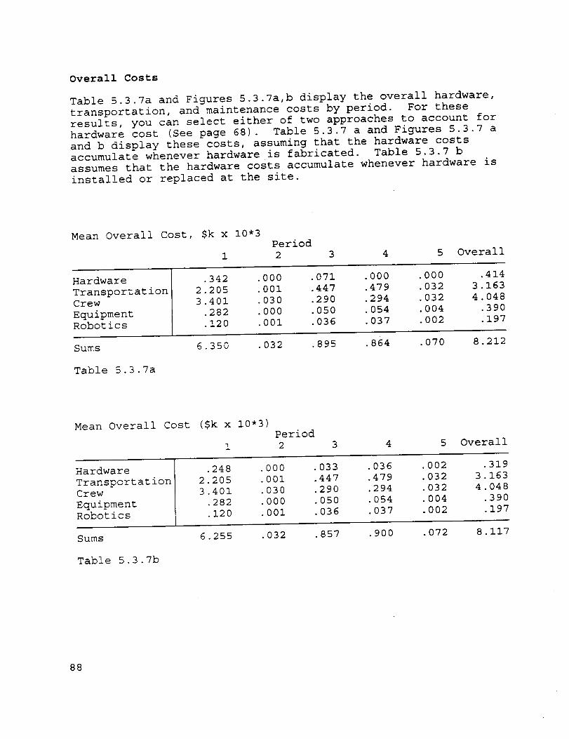
Overall Costs

Table 5.3.7a and Figures 5.3.7a,b display the overall hardware,

transportation, and maintenance costs by period. For these

results, you can select either of two approaches to account for

hardware cost (See page 68). Table 5.3.7 a and Figures 5.3.7 a

and b display these costs, assuming that the hardware costs

accumulate whenever hardware is fabricated. Table 5.3.7 b

assumes that the hardware costs accumulate whenever hardware is

installed or replaced at the site.

Mean Overall Cost, $k x 10"3Period

1 2 3 4 5 Overall

Hardware

Transportation

Crew

EquipmentRobotics

.342 .000 .071 .000 .000 .414

2.205 .001 .447 .479 .032 3.163

3.401 .030 .290 .294 .032 4.048

.282 .000 .050 .054 .004 .390

.120 .001 .036 .037 .002 .197

Sums

Table 5.3.7a

6.350 .032 .895 .864 .070 8.212

Mean Overall Cost ($k x 10"3)Period

1 2 3 4 5 Overall

Hardware

Transportation

Crew

EquipmentRobotics

.248 .000 .033 .036 .002 .319

2.205 .001 .447 .479 .032 3.163

3.401 .030 .290 .294 .032 4.048

.282 .000 .050 .054 .004 .390

.120 .001 .036 .037 .002 .197

Sums

Table 5.3.7b

6.255 .032 .857 .900 .072 8.11v

88

0

g(

m

I

.°.°o

. .</_-.-.:_... t//_•.-.;_//,.. _,_,:. o

.. _.;_• .-- k_:,i,:i.. [-2_"

_.:--_-.-.- -.-.-.-.-.-...-.=================================================================================_--,.:._,............. _:i::_;..',-::.>-:.._,_._-/._/,.:/.% ...::,:..:/._:.-._._,,::/..,...-:::.._......,F::-:_-..-- - '" " " i_:?-_:>.:_-_'-:_:_-'>.;_::;::_i_:::?-:i-':_:?:'._:_;_':_!...."-'"_I_-.-:::_.-..'.-.'-. ".'.'.'._.-'/:._.",.://'/',_:.::."_::_._':,;.,:/,':,'4,?/.4,;,_,',4.-;.__:.____-._ " " " - . .r-"-......,.-,-'..-.v,;-,.-,...-.-.,,.,',-,..-'.- :.,-.."-.'--'-"_i--'_;-__............ [`_._:_::..;:/_..:-`..._.;..;.._..;._..-_._.::_.'.>.:.....:_'.:.f_.>::':;_._;::<--:-;;-_1

//./, :Ii::--:::3....,.-- ..... _-_,>:_._-_'_:,_:_, ""................ r/,"/','."-'/'-'--,'," _-"_"/."-'."_"" .'*_'-'-_'/'-""" " _'---'..'.

_-':-':'I ......... , _ ......... "_ ............ 1 "'_ I

0_a,,,nll

ID

,,u-i

©0

0

_0

3_

D-

0

,3:

89

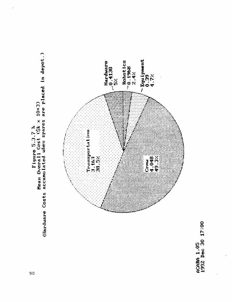
0

,:,:,4

U

,r.,,i

C_-_

_U_UU

0

IU

n_

9O

C__e

C_

-U,v,,_ID

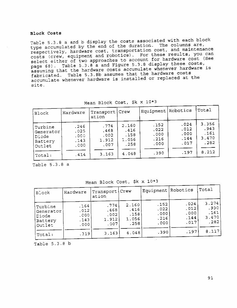
Block Costs

Table 5.3.8 a and b display the costs associated with each block

type accumulated by the end of the duration. The columns are,

respectively, hardware cost, transportation cost, and maintenance

costs (crew, equipment and robotics). For these results, you can

select either of two approaches to account for hardware cost (See

page 68). Table 5.3.8 a and Figure 5.3.8 display these costs,

assuming that the hardware costs accumulate whenever hardware is

fabricated• Table 5.3.8b assumes that the hardware costs

accumulate whenever hardware is installed or replaced at the

site.

Mean Block Cost, $k x 10"3

Block

Turbine

Generator

Diode

Battery

Outlet

Total :

Hardware

.246

.025

.000

.143

.000

.414

Transport

ation

.774

.468

.002

1. 912

.007

3.163

Crew

2.160

.416

.158

1.056

.258

4.048

Equipment

.152

.022

.000

.216

.000

•390

Robotics

.024

.012

.000

•144

.017

.197

Total

3.356

.943

.161

3.470

.282

8 •212

Table 5.3.8 a

Mean Block Cost, $k x 10"3

Block

Turbine

Generator

Diode

Battery

Outlet

Total:

Hardware

.164

.012

.000

.143

.000

.319

Transportation

.774

.468

.002

1.912

.007

3.163

Crew

2.160

.416

.158

1.056

.258

4.048

Equipment

.152

.022

.000

.216

.000

.390

Robotics

•024

•012

.000

.144

.017

.197

Total

3.274

.930

.161

3.470

.282

8. 117

Table 5.3.8 b

91

_,%..',°.¸.%° ..-/°.-.o_° _ .- _

_ _'; ,.':"-':"-::-.:':-:.':4.':-• ,._ _, ",::-:;::::::::-:::s-::::-:;,::>..

i....- ¢ • .- - .-.-......+'."-:."->':.-i.'>:-":-.-'..-'

,-_ _.':".-:, .-:...-:...-:.-..-.:-:.

ii-!!i!!.!i!!-!!!i!!!.?5!!.i?-!i!i

92

III

,-:s.:,>.::.:::::.;::::.;::;:.;._:;i;.':..-....-.::,..:....,..:.,.

..'-2"..i--.-".:':/.,':-".4-;.-:..'.:-;.::,:..::-;...::,.;;;:,.:..;>;":-:.':".-"9-:,:,'-",,_:.."

_"4-';¢-_,://_//.,

,._;;;..::;,,..;,;..,1,;.,"..../,.,.,

,:..-.-;:.>-',;.,,.,,...

', .. ' ' i

I....... {{......I ....

{ ....

! ." "." ."

) ......

:. . ..- .

{......

! ......

I. ". .. ".-

i ....

}

[ - " , {

! ......! .....

iii illllill .

_U

_0

0

3_

,e

U

_:_

5.4. Resource Allocations

This section deals with the quantity of depot spares and the

usage of hardware mass, volume, and maintenance time over the

duration.

Depot Supply

Table 5.4.1 displays the most probable quantity of each block

type residing in the supply depot for each block type. A barchart (Figure 5.4.1) displays the most probable quantity of

spares for a selected block type residing in storage.

Most Probable Cumulative Quantity in Supply

Period

Block Name 0 1 2 34

Turbine

Generator

Diode

Battery

Outlet

1 1 1 1 1

2 1 1 1 1

7 7 7 7 7

0 0 2 0 0

2 2 2 2 2

Table 5.4.1

93

raF,,

06

0

_.....,,.......-..,.....-............................................................_:,_,-.._-_..:_.:.:_.>:._:._::.:.,::.,.::....::-_,:____:-_-_-_,

!i!i._!!!:i:iii.:_.:::ii.i_!.:.::_i:i:._::..._:_(_:_.=:r_:__:_i:.......!;_.;_;_:.__!_:....:.:_:÷..:.:..:.:.:.:...:.,._.,,:FI':-D};":': .":'Z"" "-" "'..'." • -" ":-".'. -" ...................... ZZ_"._ ........ "_--- ..........................

0

_=_

I

: I

0

p..

U

(JP,I<I:0"_

94

Hardware Delivered

Tables 5.4.2 a and b show the most probable quantities of each

block type delivered to the site by period. Choose either of the

following options from the menu:

Resupply Includes hardware delivered for resupply

only. See Table 5.4.2 a and Figure 5.4.2 a.

Total Includes hardware delivered for both

installation and resupply. See Table 5.4.2 b

and Figure 5.4.2 b.

These quantities can be displayed as a bar chart for a single

block type, selected by the user, as in Figures 5.4.2 a and b.

Most Probable Quantity of Resupply Hardware Delivered

Period

Block Name 0 1 2 3 4 Overall

Turbine

Generator

Diode

BatteryOutlet

0 0 0 0 0 0

0 0 0 0 0 0

0 0 0 0 0 0

0 0 3 3 0 6

0 0 0 0 0 0

Table 5.4.2 a

Most Probable Quantity of Total Hardware Delivered

Period

Block Name 0 1 2 3 4 Overall

Turbine

Generator

Diode

BatteryOutlet

2 0 0 0 0 2

1 0 0 0 0 1

3 0 0 0 0 3

6 0 3 3 0 12

1 0 0 0 0 1

Table 5.4.2 b

95

C_

0

01-

I,, , l _Il ' ' ,I, ,,, I, ,,, I,, ,, I ,, , _I

• m • • • •

96 _ N I'4 _ .-_ _

r_

-o

R_N

i

J,_ "°

00_.

O'

0

0E

_-_÷_÷_ 01

C

0

00ii

p-,,-I

0

0-U

_txl_ChO0

9"/

Resource Usage

Resource usage (mass, volume, and maintenance hours) may be

tabulated with or without installation requirements. Choose

either Resupply or Total from the menu. Tables 5.4.3 through

5.4.7 show the results for the example system used throughout

this manual.

Table 5.4.3a, b

5.4.4a, b

5.4.5a, b

5.4.6a, b

5.4.7a, b

Mass

Volume

Maintenance Action #I

Maintenance Action #2

Maintenance Action #3

(Crew)

(Equipment)

(Robotics)

In each case, the row labelled "Sums" shows the total mass at

each period. The bottom row, "Constraint", shows the limit

imposed on the resource during each period. The constraints for

each resource are entered in the Logistics Constraints Table

(page 34).

The total amount for each of the above resources is displayed, by

period, as a bar chart (Figure 5.4.3 through 5.4.7).

98

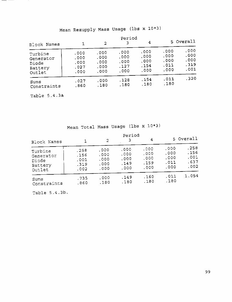
Mean Res.upply Mass Usage (ibs x 10"3)

PeriodBlock Names 1 2 3 4

5 Overall

TurbineGeneratorDiodeBatteryOutlet

.000 .000 .000 .000 .000 .000

.000 .000 .000 .000 .000 .000

.000 .000 .000 .000 .000 .000.027 .000 .127 .154 .011 .319.000 .000 .000 .000 .000 .001

Sums .027 .000 .128 .154 .011Constraints .860 .180 .180 .180 .180

Table 5.4.3a

.320

Block Names

Mean Total Mass Usage (ibs x 10"3)

Period1 2 3 4 5 Overall

TurbineGeneratorDiodeBatteryOutlet

.258 .000 .000 .000 .000 .258.156 .000 .000 .000 .000 .156.00! .000 .000 .000 .000 .001.319 .000 .149 .159 .011 .637.002 .000 .000 .000 .000 .002

Sums .735 .000 .149 .160 .011Constraints .860 .180 .180 .180 .180

Table 5.4.3b.

1.054

99

i00

×

mE

E

A

_-_.-_.._-T,_-:T.•--..--_.._-.

I i I

N

I-!

C,

C_

0

00

p-

-U_0

U_

Lf_

×

l

.,_ T"

I

A :0

!

i I I I i' 1

O_

N

0

E

0

p..

_N_:__,.__'_

i01

Block Names

Mean Resupply Volume Usage (ft3)

Period

1 2 3 4 5 Overall

Turbine

Generator

Diode

BatteryOutlet

.000 .000 .000 .000 .

.000 .000 .000 .000 .

.420 .196 .084 .ll2 .

3.400 .000 16.320 19.720 i.

.000 .080 .160 .080 .

00O

000

140

360

000

.000

.000

.952

40.800

.320

Sums

Constraints

Table 5.4.4a

3.820 .276 16.564 19.912 1.500

150.000 30.000 30.000 30.000 30.000

42.072

Block Names

Mean Total Volume Usage (ft3)

Period

1 2 3 4 5 Overall

Turbine

Generator

Diode

BatteryOutlet

68.400 .000 .000 .000 .000 68.400

22.600 .000 .000 .000 .000 22.600

1.260 .196 .084 .112 .140 1.792

40.800 .000 19.040 20.400 1.360 81.600

.800 .080 .160 .080 .000 1.120

Sums

Constraints

Table 5.4.4b

133.860 .276 19.284 20.592 1.500

150.000 30.000 30.000 30.000 30.000

175.512

102

£

°l,,_

.:>12; "f"

r._

T-

:> c,-i ::; £ _

;)

D

_o

=_,_

F1

U

103

,,_ ,...,

U'_::> "_

_ .-,.,

,..,..,_

0

,,ml

OP

t I ' J t i f I I I I i I I

,0 _ 0

v-I

0

U

0

B

=

=

U

(JN

104

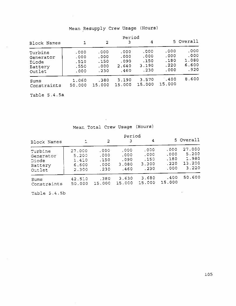
Mean Resupply Crew

Block Names 1 2

Usage (Hours

Period

3 4 5 Overall

Turbine

Generator

Diode

Battery

Outlet

.000

.000

.510

.550

.000

.000 .000 .000 .000 .000

.000 .000 .000 .000 .000

.150 .090 .150 .180 1.080

.000 2.640 3.190 .220 6.600

•230 .460 .230 .000 .920

Sums 1.060 .380

Constraints 50.000 15.000

Table 5.4.5a

3.190 3.570

15.000 15.000

.400

15.000

8.600

Block Names

Mean Total Crew Usage (Hours)

Period

! 2 3 4 5 Overall

Turbine

Generator

Diode

Battery

Outlet

27.000 .000 .000 .000 .000

5.200 .000 .000 .000 .000

1.410 .150 .090 .150 .180

6.600 .000 3.080 3.300 .220

2.300 .230 .460 .230 .000

27.000

5.200

1.980

13.200

3.220

Sums

Constraints

Table 5.4.5b

42.510 .380 3.630 3.680 .400

50.000 15.000 15.000 15.000 15.000

50.600

I05

Ul 0• ;q

=

d,o + ,

I

ItI

E._X.2a..2_ M

1NNt_

N

U

0

=

=

.i

,el

U

106

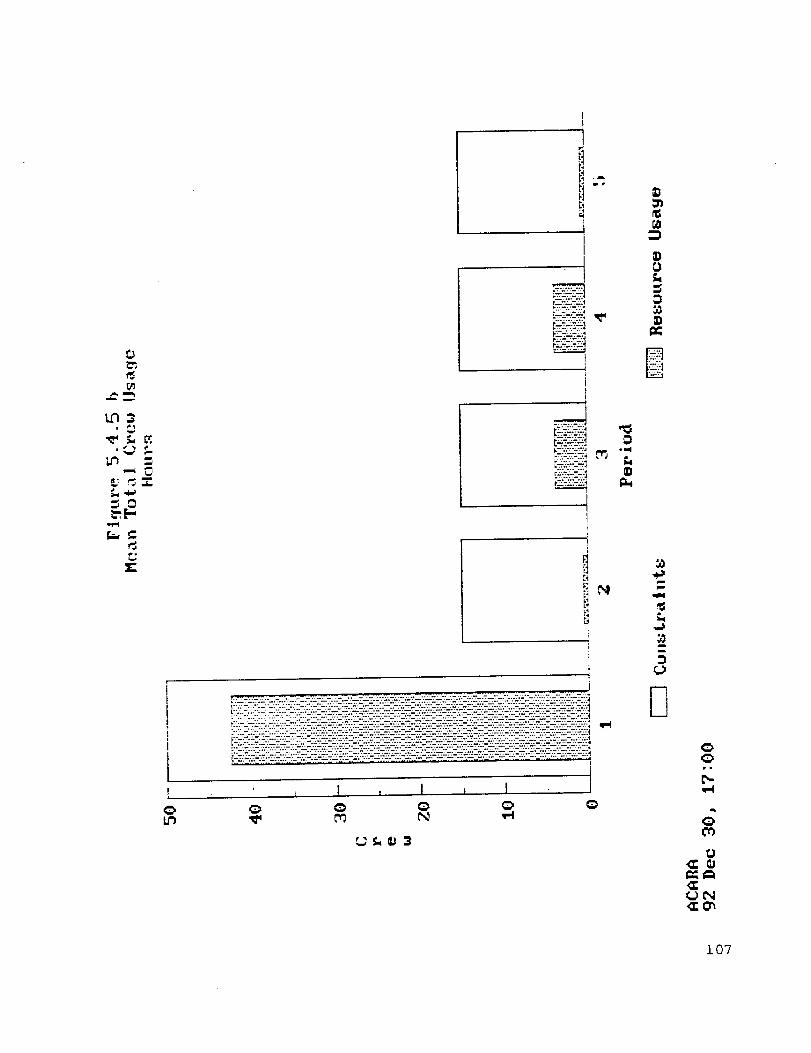
0

l,.,n _

. (,._ e,f..

f,.+.,._

_,, E--,it_t

i

i

i

L!i

I

Il

_._--+,:4.Z:,<_........ .,Jc.:_m _-_ _,

i. .........

i. u._-.+o?-.u;

,+

m

v::x:_+-+'_':°'1 Ik4_::._.+++_.+.--++,

i

+.I,.,,,i

_j

;o. ...............

............ ..+--.+......, ......... + v-_---_-._-..--.:..:-_-.?.:.-:',._.-.__-..?.'_'".. -'- .. .................... ,.:,:._.7,;,.-,_.;_.-2:_.-"...-.-'_.--:.;_...-:,-._.--............. - .................

-,-,++.-,w. '..':"--_- -:; -.+_, -_. --. ,.-.,.:.- -.-+.+.:-_A-,.+:+':-.m- -._.v.:.;,w+:.'."

i::_:::±.:..::_:+:"_:;:.:.:_:.e...:..:-_.z.:.:_:._.._+_z;-._.:_:._._.-_._-.+_.:::.:.+.:_g...:._?._.z.-:#_:::_-:_:.:_:_:._.::-_-:.±::.`..:._-_:.:_,...................... .+ -_±--_--+-_u++"u...... .'" • .....i

:::::::::::::::::::::::.z-::-:_:+:_:+::.........................-.....--,+-.......................

,,.<

mIoo

to

IIIII

r.,

Dgh

D<_

le

C_

0')

<__N

107

Block

Mean Resupply Equipment Usage

PeriodNames 1 2 3

(Hours)

4 5 Overall

TurbineGeneratorDiodeBatteryOutlet

.000 .000 .000 .000 .000 .000

.000 .000 .000 .000 .000 .000

.000 .000 .000 .000 .000 .000

.450 .000 2.160 2.610 .180 5.400

.000 .000 .000 .000 .000 .000

Sums .450 .000 2.160 2.610 .180Constraints 16.000 6.000 6.000 6.000 6.000

Table 5.4.6a

5.400

Mean Total Equipment

Block Names 1 2

Usage

Period3

(Hours)

4 5 Overall

TurbineGeneratorDiodeBatteryOutlet

7.600I.i00

.0005.400

.000

.000

.000

.000

.000

.000

.000

.000

.000

2.520

.000

.000

.000

.000

2.700

.000

.000

.000

.000

.180

.000

7.600

i. I00

.000

10.800

.000

Sums

Constraints

Table 5.4.6b

14.100

16.000

.000

6.000

2.520

6.000

2.700

6.000

.180

6. 000

19.500

108

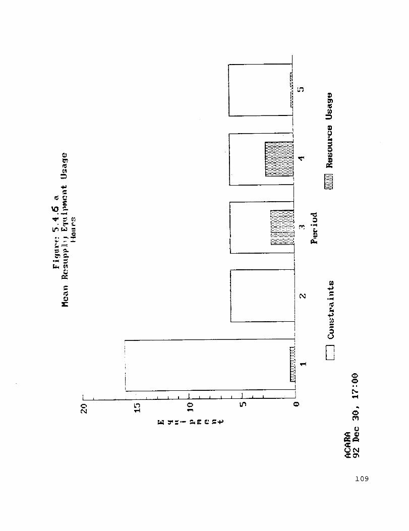
_0_

tI L

_4L_

IJ

I

J

ii

I

i L _ I i i i , ] i I,

N

II

_0

t3

0

= ,,,.II

D

=

=:)

r.3

0

_N

109

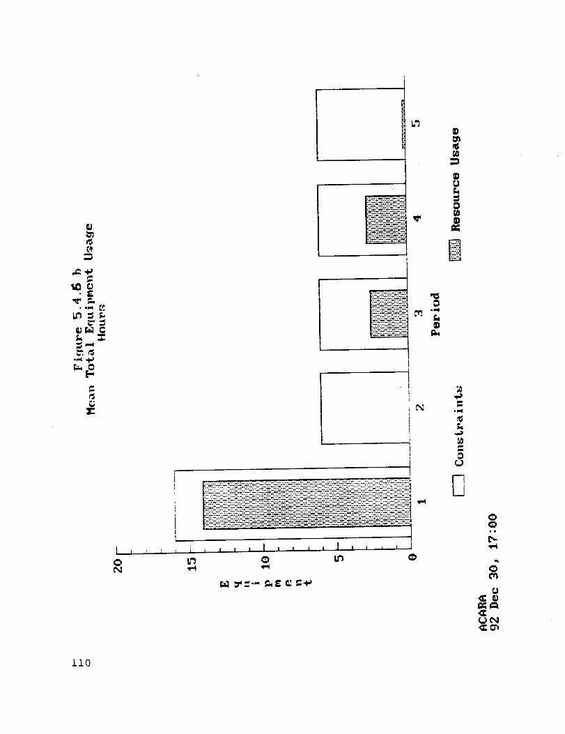
t_

1,0,g.£

t_C-',-iiii

i

;,.._t• ,_-. _z,..it.._-.z -,

_.4.'_+_

................................ _.:_...............................:.;:.:.__...:._:.::::...::::--_<._E_...:_;

iI i ', _ , i _ I I i I i I I | _ ! I _ I

Lt_

r._ __--'-,- _ _ _..i_

_D

Q)

t_ID

[]Qii

L",..

t_

t,.) IN

ii0

Block Names

Mean Resupply Robotics Usage

Period1 2 3

(Hours)

5 Overall

TurbineGeneratorDiodeBatteryOutlet

.000 .000 .000 .000 .000 .000

.000 .000 .000 .000 .000 .000

.000 .000 .000 .000 .000 .000

.150 .000 .720 .870 .060 1.800

.000 .030 .060 .030 .000 .120

SumsConstraints

Table 5.4.7a

.150 .030 .780 .900 .060299997 299997 299997 299997 299997

1.920

Block Names

Mean Total Robotics Usage (Hours)

Period1 2 3 4 Overall

TurbineGeneratorDiodeBatteryOutlet

.600 .000 .000 .000 .000 .600

.300 .000 .000 .000 .000 .300

.000 .000 .000 .000 .000 .0001.800 .000 .840 .900 .060 3.600

.300 .030 .060 .030 .000 .420

SumsConstraints

Table 5.4.7b

3.000 .030 .900 .930 .060299997 299997 299997 299997 299997

4.920

iii

t,,,:f

mm

ID

I",,,,,,• t/l

• _lml

1,1"i.,I,,J'0

t,,,O

tD

IUE

_+"'-':'E÷:-.....................................

I"t.; ...........................................

tn

i

A

I IN

_e-..]

0

r,l

0

0

m

0U

S

p,.

-U

U_

112

r_

.5o

i1.I

_-._

_0

._0

mm_i

T-

Z---:+--+S-.'+'_÷ "r:+S +-'t÷---:'--+_ ":_,'r" - ,..; :1.-.::7 ...... -:_:-Z:--:---'"

'_+%.-t._;--_-r.v.-r'._.-'._'r._ .....

1

L i ,, _ i I _ ! I I i I I i I t l I 1 I

p';

l'Xl

.................. ii_

i_lllil Itl

"00

0

0

0

_a

0

Fl0

-(.1

_N

113

5.5 Results Files

The results of ACARA analyses are stored into "results files" for

future use. These files have the extension *.ARI. Each results

file contains the output data needed to create each of the tables

in the Results Menu as well as the input data needed to repeat

the calculation. A Results file is automatically saved after

each simulation during Batch mode simulation. The Results Files

menu allows you to load, save, copy, delete, and rename files.

The steps are identical to those for system files. Refer Section

3.8, page 37).

When a results file is retrieved, ACARA loads the input as well

as the results. You may then change the data and repeat the

simulation using Immediate mode.

114

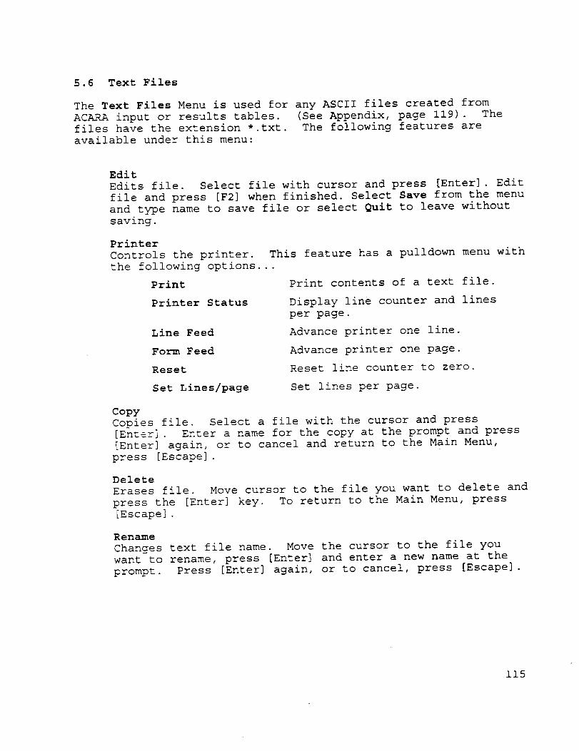
5.6 Text Files

The Text Files Menu is used for any ASCII files created from

ACARA input or results tables. (See Appendix, page 119). The

files have the extension *.txt. The following features are

available under this menu:

Edit

Edits file. Select file with cursor and press [Enter]. Edit

file and press [F2] when finished. Select Save from the menu

and type name to save file or select Quit to leave without

saving.

Printer

Controls the printer.

the following options...

Print

Printer Status

Line Feed

Form Feed

Reset

Set Lines/page

This feature has a pulldown menu with

Print contents of a text file.

Display line counter and lines

per page.

Advance printer one line.

Advance printer one page.

Reset line counter to zero.

Set lines per page.

Copy

Copies file. Select a file with the cursor and press

[Enter]. Enter a name for the copy at the prompt and press

[Enter] again, or to cancel and return to the Main Menu,

press [Escape].

Delete

Erases file. Move cursor to the file you want to delete and

press the [Enter] key. To return to the Main Menu, press

[Escape].

Rename

Changes text file name. Move the cursor to the file you

want to rename, press [Enter] and enter a new name at the

prompt. Press [Enter] again, or to cancel, press [Escape].

115

Acknowledgements

Acknowledgement is made to the following people for their

contributions to the ACARA algorithms and software:

Bream, Bruce

Carr, Thomas

Dorcey, James

Hoffman, David

Sa!cido, Ann

Shiller, Jonathan

Viterna, Larry

Zampino, Edward

NASA Lewis Research Center

Case Western Reserve University

Science Applications

International Corporation

NASA Lewis Research Center

Stanford University

Case Western Reserve University

NASA Lewis Research Center

NASA Lewis Research Center

116

Appendix

A. Input Windows

Input windows are used to enter ACARA input parameters.

chart below explains how to use the input windows.

The

Move cursor right to the next field:

Move cursor left to the previous

field:

Leave window and save your entries:

Press [Enter] or

[_Tab]. .

Press [_Tab] .

Press [F2] or [Enter]

(if cursor is at last

field. )

Leave window and cancel all entries: Press [Escape].

Read help to explain the data to be Move cursor to the

entered in an input field: appropriate input field

and press [FI] .

117

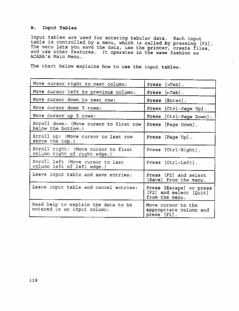
B. Input Tables

Input tables are used for entering tabular data. Each input

table is controlled by a menu, which is called by pressing [F2].

The menu lets you save the data, use the printer, create files,

and use other features. It operates in the same fashion asACARA's Main Menu.

The chart below explains how to use the input tables.

Move cursor right to next column:

Move cursor left to previous column:

Move cursor down to next row:

Move cursor down 5 rows:

Move cursor up 5 rows:

Scroll down: (Move cursor to first row

below the bottom.)

Scroll up: (Move cursor to last row

above the top.)

Scroll right: (Move cursor to first

column right of right edge.)

Scroll left (Move cursor to last

column left of left edge.)

Leave input table and save entries:

Leave input table and cancel entries:

Read help to explain the data to be

entered in an input column:

Press [_Tab].

Press [_Tab].

Press [Enter].

Press [Ctrl-Page Up].

Press [Ctrl-Page Down].

Press [Page Down].

Press [Page Up].

Press [Ctrl-Right] .

Press [Ctrl-Left].

Press [F2] and select

[Save] from the menu.

Press [Escape] or press

[F2] and select [Quit]

from the menu.

Move cursor to the

appropriate column and

press [FI] .

118

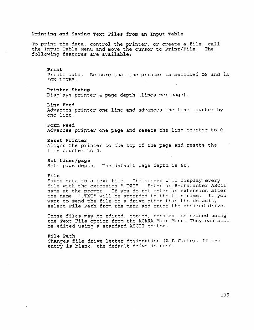
Printing .and Saving Text Files from an Input Table

To print the data, control the printer, or create a file, call

the Input Table Menu and move the cursor to Print/File. The

following features are available:

Print

Prints data.

"ON LINE".

Be sure that the printer is switched ON and is

Printer Status

Displays printer & page depth (lines per page).

Line Feed

Advances printer one line and advances the line counter by

one line.

Form Feed

Advances printer one page and resets the line counter to 0.

Reset Printer

Aligns the printer to the top of the page and resets the

line counter to 0.

Set Lines/page

Sets page depth. The default page depth is 60.

File

Saves data to a text file. The screen will display every

file with the extension ".TXT". Enter an 8-character ASCII

name at the prompt. If you do not enter an extension after

the name, ".TXT" will be appended to the file name. If you

want to send the file to a drive other than the default,

select File Path from the menu and enter the desired drive.

These files may be edited, copied, renamed, or erased using

the Text File option from the ACARA Main Menu. They can also

be edited using a standard ASCII editor.

File Path

Changes file drive letter designation (A,B,C,etc). If the

entry is blank, the default drive is used.

119

Other Features

The Production Quantities and Logistics Constraints input tables

often extend beyond the left and right edges of the screen. They

have the following options in the first section of the input

table menu to make data entry easier.

Copy Column

Copies the values from the column at the cursor to those

columns right of the cursor. Move the cursor to that

column, select the Copy Column option from the Input Table

Menu, and press [Enter].

Move to Column

Moves the cursor directly to a column. Select the Move to

Column option, move the cursor to the appropriate column

heading from the pulldown menu, and press [Enter].

Some input tables have a third menu section entitled Modify

Table, for inserting, copying, or cutting/pasting rows of data.

This menu includes one or more of the following:

InsertInserts rows in the table. Move the cursor to the desired

location, press [Enter] and move the cursor until the

desired number of rows are displayed in reverse video. Press

[Enter] again to insert the rows.

CutRemoves one or more rows. Move cursor to the first line you

want to remove, press [Enter] and move cursor to mark the

desired number of rows in reverse video. Press [Enter] again

to remove these rows.

The rows you most recently cut may be inserted elsewhere in

the table using Paste (if available in the editor.)

Undo

Undoes most recent change to data done by the Insert, Cut,

Paste, or Copy options. Select Undo from the menu and press

[Enter].

Copy

Copies one or more rows. Move cursor to 1st row you want to

copy and press [Enter]. Move the cursor down until all of

these rows appear in reverse video and press [Enter]. Move

the cursor to the desired destination and press [Enter] to

copy the rows.

120

Paste

Inserts most recently 'Cut' rows into data table. First,

use Cut to remove these rows from the table. Then, using

Paste, move the cursor to the desired destination in the

table and press [Enter] to insert the rows.

The following chart shows the input tables which have one or more

of the options in the Modify Table section described on the

previous page. An "X" indicates that the feature is included.

Input tables not listed in this chart have none of thesefeatures.

Insert Cut Undo Copy Paste

Names & Properties X X X X X

Block Numbers X X X

Initial Ages X X X

Installation Times X X X

Block Diagram X X X

Redundancy X X X

121

C. Displaying Output

The following chart explains how to control the display screen

for ACARA's output tables under the Results menu:

Scroll up or down: Press [Page Up] or [Page down].

For very large tables that "wrap"

across the screen, [Page Up/Down]

will scroll from section to

section.

Jump to top of table: Press [Home].

Jump to bottom of table: Press [End].

Move cursor up or down 5 Press Ctrl-[Page Up/Down].

rows.

Leave the display screen and Press [Escape].

return to the Main Menu:

Print the table: Press [F2] and select Print from

the Print/File Menu (See

Appendix, page 119.)

Save the table as a text Press [F2] and select File from

file: the Print/File Menu (See

Appendix, page 119.)

Display/Print Graph:

(if available)

Press [F2] and select the desired

graph from the Graphics Menu. To

print the graph, press [P] whileit is still visible.

Important: A dot-matrix printer

(e.g., Epson) is required to

print graphs.

122

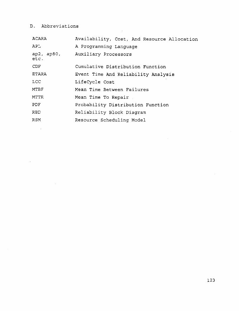
D. Abbreviations

ACARA

APL

ap2, apS0,etc.

CDF

ETARA

LCC

MTBF

MTTR

PDF

RBD

RSM

Availability, Cost, And Resource Allocation

A Programming Language

Auxiliary Processors

Cumulative Distribution Function

Event Time And Reliability Analysis

LifeCycle Cost

Mean Time Between Failures

Mean Time To Repair

Probability Distribution Function

Reliability Block Diagram

Resource Scheduling Model

123

Index

Active block 13, 22, 29, 30

APL2 programming language 5

Auxiliary processors 123, 5

Batch printouts 36, 53

Block Diagram Table (RBD)

Capacity 18, 28

Minimum Number of Blocks 28

Preparing RBD 9

Subsystem Elements 28

Subsystem Type 27

View Diagram 29

Block numbers 9, 17, 23-25, 28, 65, 121, i0

Input Table 9, 23

Shorthand for consecutive nos. 23-25, 28

Computation time 15, 16, 20, 39

Cost parameters 14, 16, 17, 27, 31, 36

Delay Time 65-67

Down Time 13, 20, 65-67

Early failure 12, 17, 21, 24, 36

Input Table 21

mean life 12, 21

Probability 12, 21

scale factor 12

shape factor 12, 21

ETARA 37, 123

Executable code 5, 7

Failure free period 24

Failure Results

Accumulated Early, Random, and Wearout Failures

64

Criticality 63

Early, Random, and Wearout Failures by Period 58Failure CDF 57

Failure PDF 54

Failures/year by Block Type 66Individual Blocks 65

Failure Results Charts

Early, Random, and Wearout Failures by Period 59

Failure PDF, All Periods 56

Failure PDF, Single Period 55

Graphics Menu 122

Help windows 8

Initial age 12, 24

Input Table 12, 24

Input Tables

Copy Columns 32, 34, 120

Copying Rows 120

Cutting Rows 120

Inserting Rows 23-25, 28, 120

124

Pasting Rows 121Printer Control 119Scrolling Right/Left 32Summary Chart of FeaturesText files 119Undo 120

Input windows 14, 117Installation time 9, 25, 26

Input Table 9, 25Lifecycle Costs

Hardware Costs 68

Maintenance 76, 79, 82

Total Cost vs Time 85

Total Costs 88, 91

Transportation Costs 73

Lifecycle Costs Charts

Hardware costs 69-72

121

Maintenance Costs 77, 78, 80, 81, 83, 84

Overall Cost by Resource Type 89, 90

Total Costs 86, 87

Total Costs by Block 92

Transportation Costs 74, 75

Local Spares 13, 31, 33

Menu system 6

MTTR 13, 16, 17, 20, 36, 123

Repair Time and Personnel Input Table 20

Names and Properties Input Table 9, 18

Capacity 18Cost 18

Mass 18

Name 18

Volume 18

Nomenclature 16, 20, 35

Parameters

Capacity Increment 15

Duration 15

Normalizing Capacity 16

Number of Runs 15

Period Length 15

Resupply Interval 15Performance Charts

Cumulative System Availability 43, 44

Equivalent Availability 46

Reliability 49-51Performance Results

Continuous State Behavior 52

Cumulative System Availability 42

Equivalent Availability 45

Overall Availability Summary 47

Reliability 48

State Availability 41

Time at Capacity 40

125

Personnel 13, 17, 20Printer 5, 39, 115, 118, 119, 122Production Quantities 13, 31, 32, 34, 36, 39, 68, 120

Input Table 32Random failure 12, 13, 22, 24, 30

Dormant MTBF Factor 13, 22, 30Input Table 12, 22MTBF 12, 13, 22, 30

Redundancy 13, 27, 30, 36, 121, 22Input Table 13, 30

Reliability 2, 9, 12, 15, 48-51, 53, 123Repair Results

Repair PDF 60Repair Results Charts

Repair PDF, All Periods 62Repair PDF, Single Period 61Single Period 61

Resource AllocationsDepot Supply 93Hardware Delivered 95Resource Usage 98

Resources Input 13, 31Local Spares 33Logistics Constraints 34

Production Quantities 32

Resupply Cutoff 34

Resources Results Charts 94, 96, 97, I00, I01, 103,

104, 106, 107, 109, Ii0, 112, 113

Results files 6, 38, 39, 114

Resupply cutoff I, 2, 13, 15, 26, 31, 32, 34, 39, 73,

95, 98, 99, 102, 105, 108, iii

Simulation by Batch Mode or Immediate Mode 38

Simulation Parameters 15

Standby block 13, 22, 29, 30

Subsystem numbers i0, 27, 28

Subsystem Types

Binary M-of-N 9, I0, 28

Parallel 9, i0, 27

Series 9, 10, 27

Variable M-of-N i0, 28

System files 6-8, 14, 17, 27, 31, 37, 38, 114

Text files 6, 39, 115, 119

Units 14, 16-18, 27, 31, 35

Wearout failure 12, 13, 22, 24, 30, 36

Input Table 22

mean Life 12, 22

scale factor 12

shape factor 12, 22

Weibull function 2, 12, 20-22

126

FormApprovedREPORT DOCUMENTATION PAGE OMBNo.0704-0188

Public reporting burden for this collastion of information is estimated to average 1 hour pet" response, including the time for reviewing inslructlo¢_, sea/ctlin 9 exis_ dalai sources,gathenng and maintaining the data needed, and oompl_ng and reviewing the coaection of inf--. Send comments regarding this burden eetimme or any other aspect of thiscollection of information, including suOgas'_ons for reducing this burden, to Washington Headquarte_ Services, Directorate for Information Operations and Reports, 1215 JeffersonDavis Highway, Suite 1204, Arlington, VA 22202.4302, and to the Office of Management and Budget, Paperwork Reduction Project (0704-0188), Washlngton, DC 20503.

1. AGENCY USE ONLY (Leave b/ank) 2. REPORT DATE 3. REPORT TYPE AND DATES COVERED

August 1993 Technical Memorandum5. FUNDING NUMBERS4. TITLE AND SUBTITLE

ACARA User's Manual

6. AUTHOR(S)

Dale K. Stalnaker

7. PERFORMING ORGANIZATION NAME(S) AND ADDRESS(F.S)

National Aeronautics and Space Administration

Lewis Research Center

Cleveland, Ohio 44135-3191

9. SPONSORING/MONITORING AGENCY NAME(S) AND ADDRESS(ES)

National Aeronautics and Space Administration

Washington, D.C. 20546-0001

WU-474-12-10

8. PERFORMING ORGANIZATION

REPORT NUMBER

E-8014

10. SPONSORING/MONITORING

AGENCY REPORT NUMBER

NASA TM- 106277

11. SUPPLEMENTARY NOTES

Responsible person, Dale K. Stalnaker, (216) 433-5399.

12a. DISTRIBUTION/AVAJLABILn'Y STATEMENT

Unclassified - Unlimited

Subject Category 38

12b. DISTRIBUTION CODE

13. ABSTRACT (Maximum 200 words)

ACARA (Availability, Cost, And Resource Allocation) is a computer program which analyzes system availability,

lifecycle cost (LCC), and resupply scheduling using Monte Carlo analysis to simulate component failure and

replacement. This manual was written to:

(1) Explain how to prepare and enter input data for use in ACARA.

(2) Explain the user interface, menus, input screens, and input tables.

(3) Explain the algorithms used in the program.

(4) Explain each table and chart in the output.

14. SUBJECT TERMS

Availability; Reliability; Monte Carlo simulation

17. SECURITY CLASSIFICATION

OF REPORT

Unclassified

NSN 7540-01-280-5500

18. SECURITY CLASSIFICATION

OF THIS PAGE

Unclassified

19. SECURITY CLASSIFICATION

OF ABSTRACT

Unclassified

15. NUMBER OFPAGES

12816. PRICE CODE

A0720. LIMITATION OF ABSTRACT

Standard Form 298 (Rev. 2-89)

Prescribed by ANSI Std. Z39-18298.1 ,,',-_

127

Nationa| _ 41N:ISpace Administration

Lew_ Rewareh CenterCk_and. Ohio 44135

oli_/__tmm

Iq_mltl ct,A4mMAIL

ADDRESSCORRECTIONREQUESTED

lililif

I I