AC analysis - Iowa State...

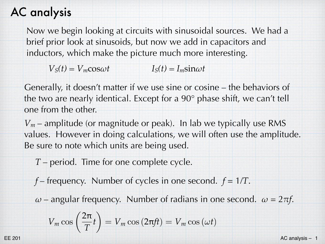
EE 201 AC analysis – 1

VS(t) = Vmcosωt

Vm – amplitude (or magnitude or peak). In lab we typically use RMS values. However in doing calculations, we will often use the amplitude. Be sure to note which units are being used.

T – period. Time for one complete cycle.

f – frequency. Number of cycles in one second. f = 1/T.

ω – angular frequency. Number of radians in one second. ω = 2πf.

9P cos

��7 W

�= 9P cos (��IW) = 9P cos (�W)

AC analysis

IS(t) = Imsinωt

Generally, it doesn’t matter if we use sine or cosine – the behaviors of the two are nearly identical. Except for a 90° phase shift, we can’t tell one from the other.

Now we begin looking at circuits with sinusoidal sources. We had a brief prior look at sinusoids, but now we add in capacitors and inductors, which make the picture much more interesting.


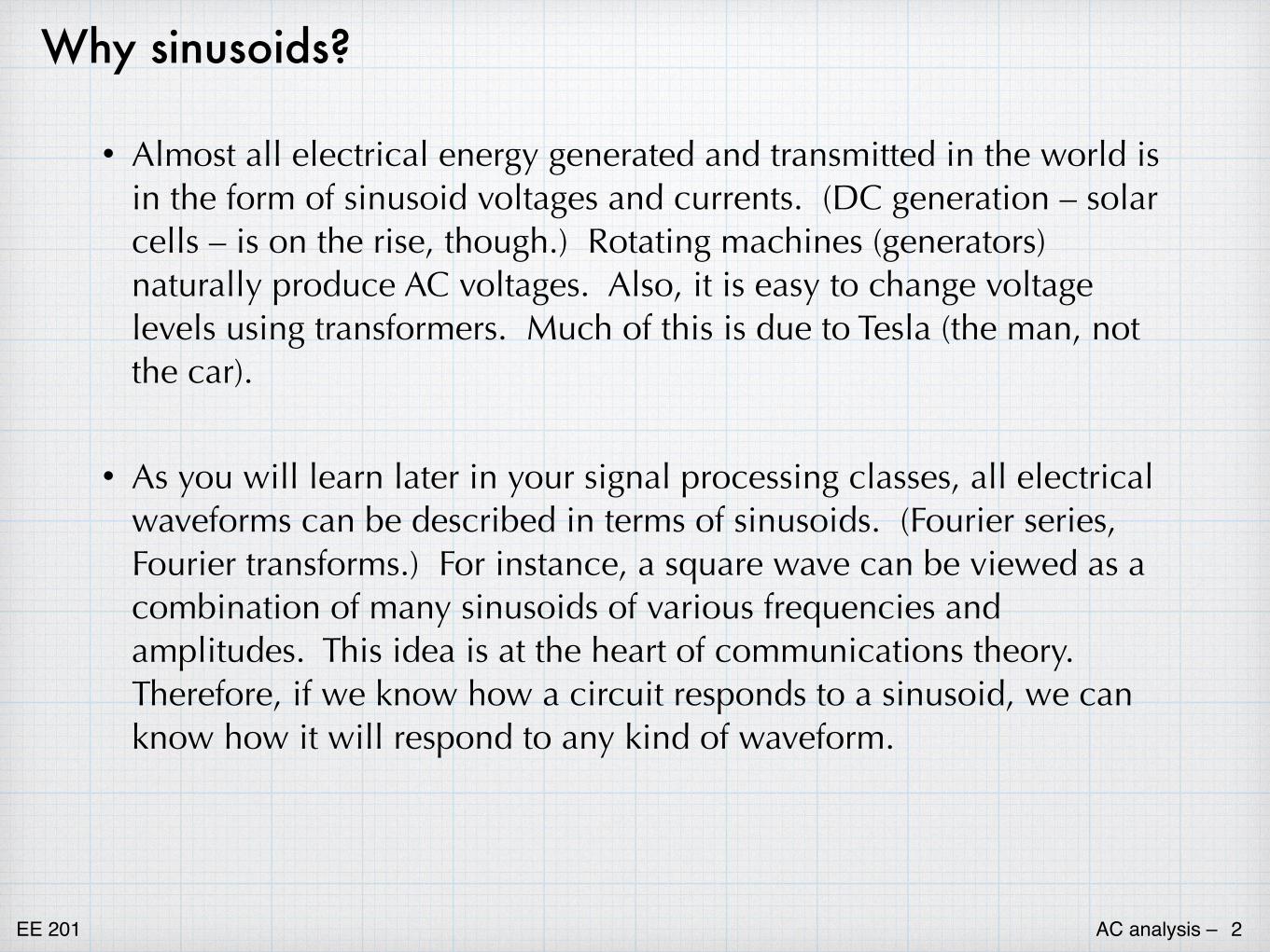
Why sinusoids?

• Almost all electrical energy generated and transmitted in the world is in the form of sinusoid voltages and currents. (DC generation – solar cells – is on the rise, though.) Rotating machines (generators) naturally produce AC voltages. Also, it is easy to change voltage levels using transformers. Much of this is due to Tesla (the man, not the car).

• As you will learn later in your signal processing classes, all electrical waveforms can be described in terms of sinusoids. (Fourier series, Fourier transforms.) For instance, a square wave can be viewed as a combination of many sinusoids of various frequencies and amplitudes. This idea is at the heart of communications theory. Therefore, if we know how a circuit responds to a sinusoid, we can know how it will respond to any kind of waveform.


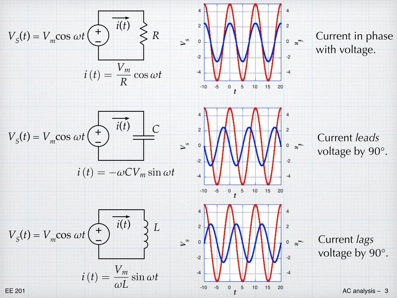
+–VS(t) = Vmcos ωt R

i(t)

L (W) =9P5 cosW

+–VS(t) = Vmcos ωt Ci(t)

L (W) = �&9P sinW

+–VS(t) = Vmcos ωt Li(t)

L (W) =9P/ sinW

Current in phase with voltage.

Current leads voltage by 90°.

Current lags voltage by 90°.


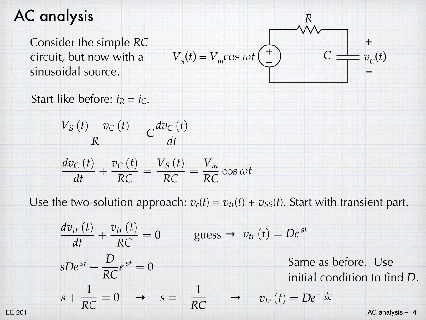
AC analysisConsider the simple RC circuit, but now with a sinusoidal source.

+–VS(t) = Vmcos ωt

R

C–

+vC(t)

Start like before: iR = iC.

VS (t) � vC (t)R = CdvC (t)

dt

dvC (t)dt +

vC (t)RC =

VS (t)RC =

VmRC cosωt

Use the two-solution approach: vc(t) = vtr(t) + vSS(t). Start with transient part.

guess →

sDe st + DRCe

st = 0

s+1RC = 0 s = � 1

RC→ →

vtr (t) = De stdvtr (t)dt +

vtr (t)RC = 0

vtr (t) = De� tRC

Same as before. Use initial condition to find D.


Now try to find a steady-state solution.

Given that the forcing function is cos(ωt), it might seem reasonable to guess something like vss(t) = Acos(ωt) and see if we find a value of A that works. Plug in the guess and try it out.

That’s not going to work. There is no value of A that can be chosen to make this equation balance out. No trig identities will help either.

Because the derivative in the steady-state equation introduces a term with sin(ωt),maybe we need to make our guess a bit more inclusive.

vss(t) = Acos(ωt) + Bsin(ωt)

Substituting this into the steady-state equation makes things a bit more complicated, but also gives us a route to a solution.

dvss (t)dt +

vss (t)RC =

VmRC cosωt

�ωA sinωt+ ARC cosωt =

VmRC cosωt


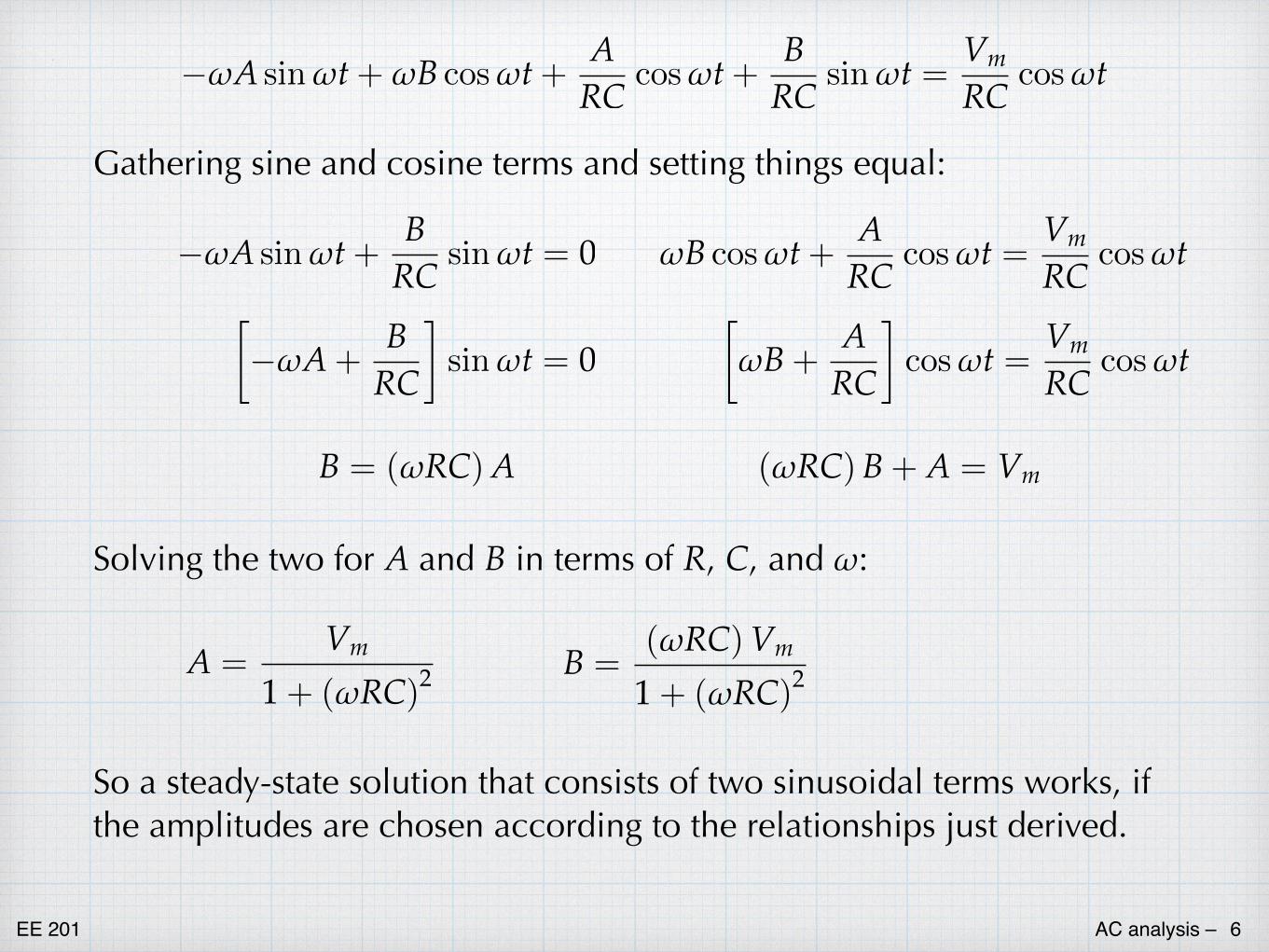
Gathering sine and cosine terms and setting things equal:

�ωA sinωt+ BRC sinωt = 0

��ωA+

BRC

�sinωt = 0

B = (ωRC)A

�ωA sinωt+ ωB cosωt+ ARC cosωt+ B

RC sinωt =VmRC cosωt

ωB cosωt+ ARC cosωt =

VmRC cosωt

�ωB+

ARC

�cosωt =

VmRC cosωt

(ωRC)B+ A = Vm

Solving the two for A and B in terms of R, C, and ω:

A =Vm

1+ (ωRC)2B =

(ωRC)Vm1+ (ωRC)2

So a steady-state solution that consists of two sinusoidal terms works, if the amplitudes are chosen according to the relationships just derived.


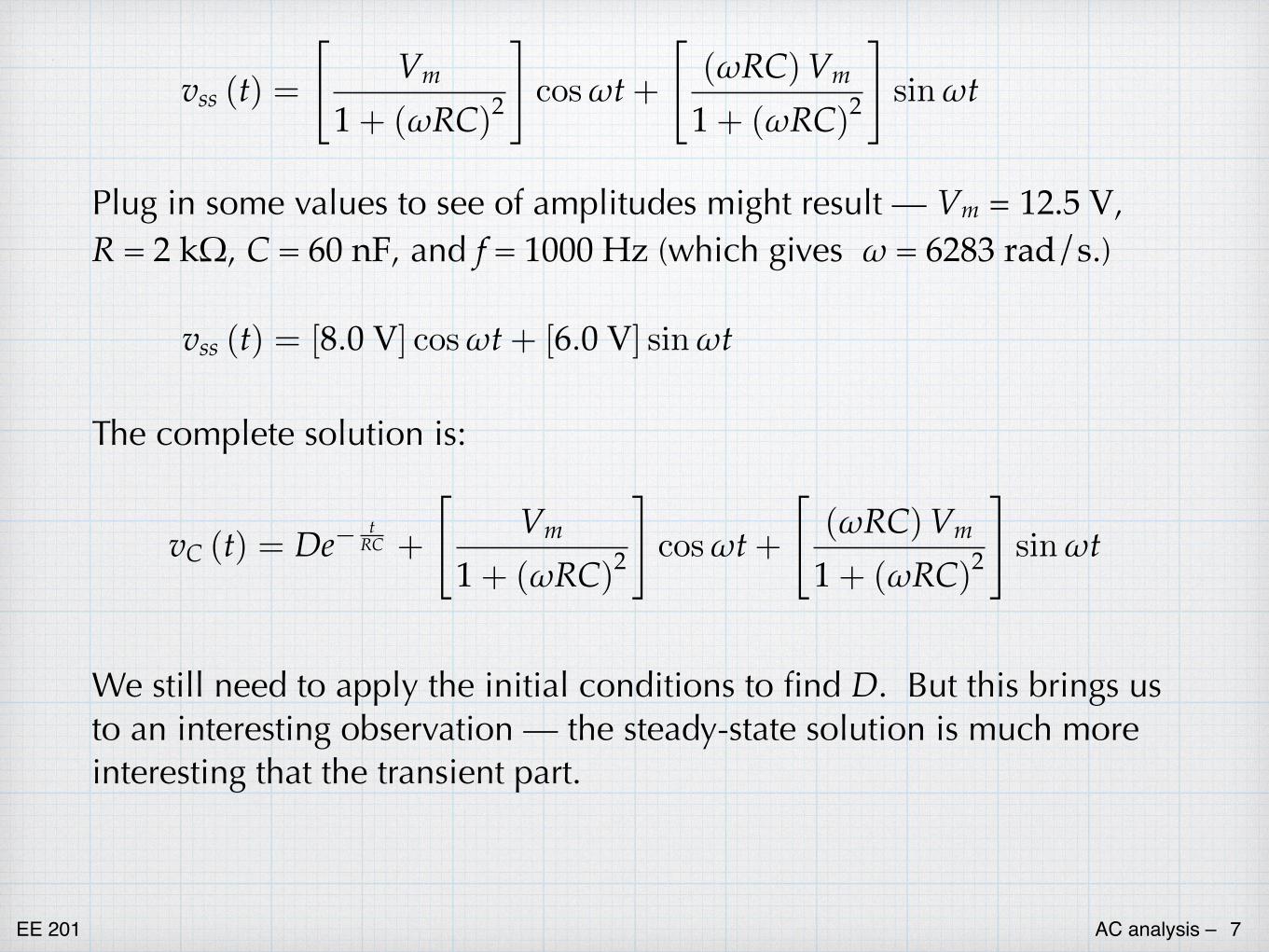
vss (t) =

�Vm

1+ (ωRC)2

�cosωt+

�(ωRC)Vm

1+ (ωRC)2

�sinωt

Plug in some values to see of amplitudes might result — Vm = 12.5 V, R = 2 k!, C = 60 nF, and f = 1000 Hz (which gives ω = 6283 rad/s.)

vC (t) = De� tRC +

�Vm

1+ (ωRC)2

�cosωt+

�(ωRC)Vm

1+ (ωRC)2

�sinωt

The complete solution is:

We still need to apply the initial conditions to find D. But this brings us to an interesting observation — the steady-state solution is much more interesting that the transient part.

vss (t) = [8.0 V] cosωt + [6.0 V] sinωt


In the step-change problem, the transient function was the only thing that was really interesting, since the forced response was just a constant.

But in the sinusoid case, the constantly changing voltage of the source will cause all of the voltages and currents in the rest of the circuit to continue changing in response. This goes on forever. Thus, the steady-state response is a very interesting part of an AC problem. In fact, it is much more interesting that the transient response, which will die away within a few moments after the circuit has started. Therefore, for the time being, we will ignore the transients and focus entirely on the steady-state solution.

Sinusoidal steady-state analysis

An added benefit of ignoring the transient response and looking only at the steady-state response is that we do not need to worry about initial conditions.

This approach of ignoring the transient function and looking only at the forced response is known in the textbooks as sinusoidal steady-state analysis. But we will call it AC analysis for short.


vss (t) =

�Vm

1+ (ωRC)2

�cosωt+

�(ωRC)Vm

1+ (ωRC)2

�sinωt

Visualizing the capacitor voltageWritten in general terms, the steady-state equation is

vss (t) = [8.0 V] cosωt + [6.0 V] sinωt

For our specific case:

Two separate sinusoids … … add to give a sinusoid.


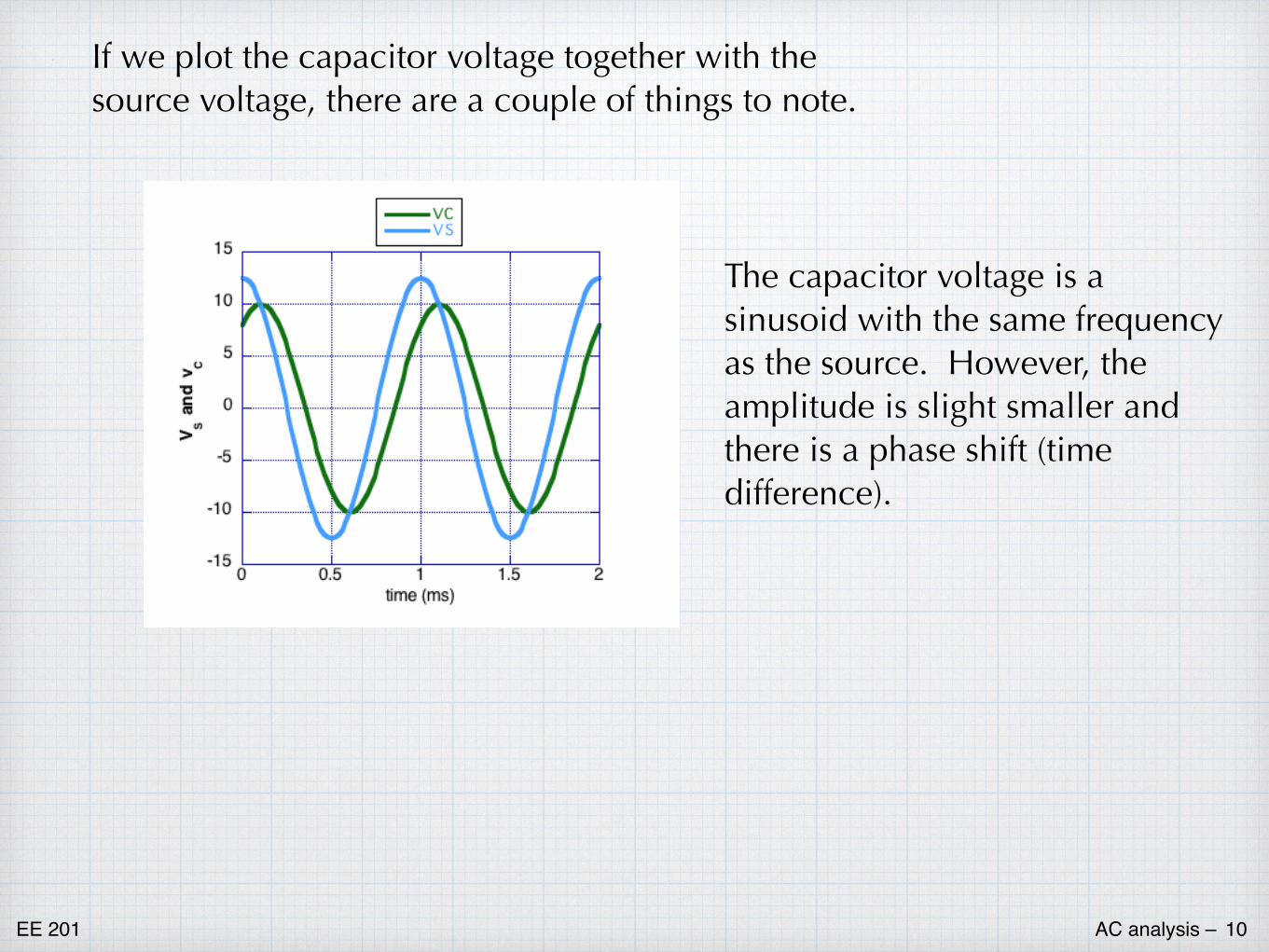
If we plot the capacitor voltage together with the source voltage, there are a couple of things to note.

The capacitor voltage is a sinusoid with the same frequency as the source. However, the amplitude is slight smaller and there is a phase shift (time difference).


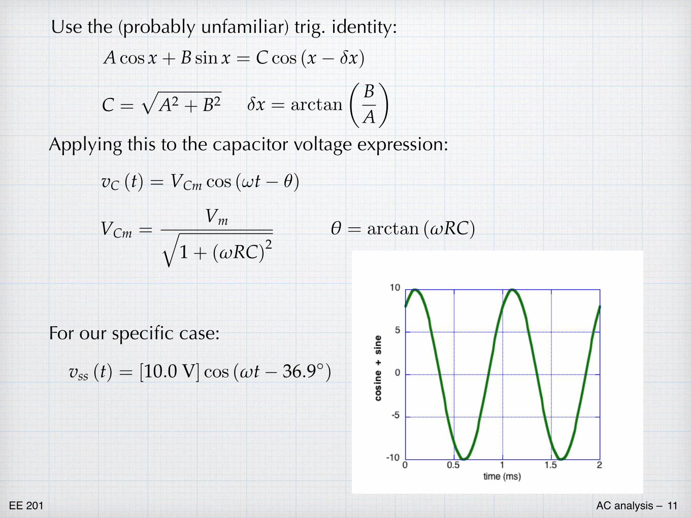
Applying this to the capacitor voltage expression:

Y& (W) = 9&P cos (�W� �)

Use the (probably unfamiliar) trig. identity:

& =�$� + %� �[ = arctan

�%$

�$ cos [+ % sin [ = & cos ([� �[)

VCm =Vm�

1+ (ωRC)2θ = arctan (ωRC)

For our specific case:

vss (t) = [10.0 V] cos (ωt � 36.9�)


We see that vC(t):

1. has time dependence of cos(ωt), just like the source,

2. has amplitude, VCm, (different from the source), and

3. has a phase shift, θ, relative to the source.

This is typical in sinusoidal circuits. All of the voltages and currents in the circuit will vary sinusoidally with the same angular frequency as the source. The problem reduces to finding the amplitude and phase shift

The problem is that the math is quite messy. Too much trigonometry. If we change the circuit, we have to start from scratch, come up with new equations, and work through the resulting trigonometry again. Bleh. It would be nice to have a simpler way to find these.


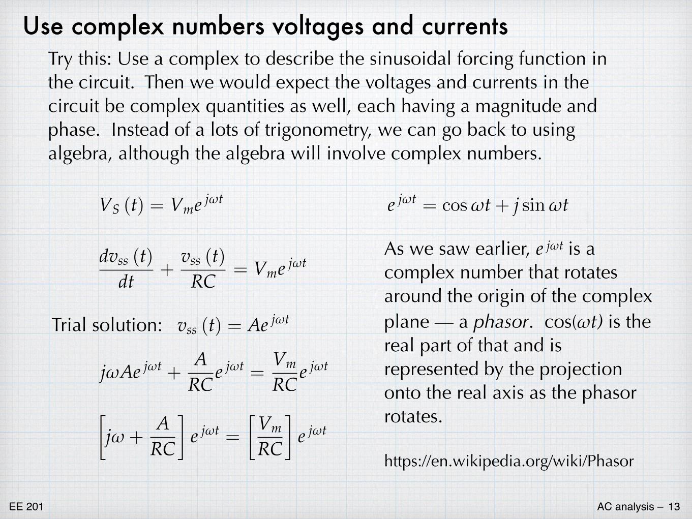
Use complex numbers voltages and currentsTry this: Use a complex to describe the sinusoidal forcing function in the circuit. Then we would expect the voltages and currents in the circuit be complex quantities as well, each having a magnitude and phase. Instead of a lots of trigonometry, we can go back to using algebra, although the algebra will involve complex numbers.

Trial solution:

VS (t) = Vme jωt

dvss (t)dt +

vss (t)RC = Vme jωt

vss (t) = Ae jωt

jωAe jωt + ARCe

jωt =VmRCe

jωt

�jω+

ARC

�e jωt =

�VmRC

�e jωt

e jωt = cosωt + j sinωt

As we saw earlier, e jωt is a complex number that rotates around the origin of the complex plane — a phasor. cos(ωt) is the real part of that and is represented by the projection onto the real axis as the phasor rotates.https://en.wikipedia.org/wiki/Phasor


�jω+

1RC

�Ae jωt =

�VmRC

�e jωt

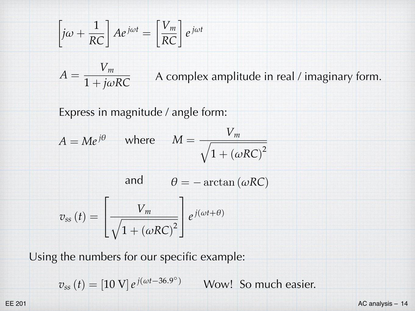
A =Vm

1+ jωRC A complex amplitude in real / imaginary form.

Express in magnitude / angle form:

A = Me jθ M =Vm�

1+ (ωRC)2where

and θ = � arctan (ωRC)

vss (t) =

�

� Vm�1+ (ωRC)2

�

� e j(ωt+θ)

Using the numbers for our specific example:

vss (t) = [10 V] e j(ωt�36.9�) Wow! So much easier.


The complex voltages and currents are sometimes known as phasors.

• In the circuit, the sinusoidal source will be described as:

9V (W) = 9P cos �W � 9V = 9PHM�W

• The voltages and currents the rest of the circuit will also be complex, having the corresponding magnitudes and phase angles with respect to the source.

Y& = 9&PHM(�W��&) � Y& (W) = 9&P cos (�W � �&)

L/ = ,/PHM(�W+�/) � L/ (W) = ,/P cos (�W + �/)


• Finally, we will drop the ejωt factor, since all voltages and currents in the circuit oscillate with the same time dependence. The same factor shows up in every single term, and so we can always divide it. Since there is no need to carry the exp(jωt) through every step in a calculation, there is really no need to include it at the beginning.

9V (W) = 9P cos �W � 9V = 9PHM��

• Like voltage, phase angle is a relative quantity – only differences are meaningful. Usually define the phase of the source to be 0°. Usually, we will express the angle in terms of degrees, but we must be able to switch back and forth between degrees and radians as we do calculations. Note that phase angle also represents a time shift.

ս =ܠ� ս = �� ӹW =

7�


impedances

+–9V

CLF

L& = &GY&GW

Y& = 96 = 9PHM�W Y&

L&=

�M�&

+

–

,6 L Y/

Y/ = /GL/GW

L/ = ,6 = ,PHM�W

Y/ = M�/,PHM�W = (M�/) L/

Y/

L/= M�/

L& = M�&9PHM�W = (M�&) Y&

+–9V R L5

L5 =Y55

Y5 = 96 = 9PHM�W

L5 =9PHM�W

5 =Y55

Y5L5

= 5


For each of the components, the ratio of complex voltage to complex current is a number. It is purely real in the case of the resistor and purely imaginary in the cases of the capacitor and inductor.

The ratios are called impedances and can be used as complex versions of Ohm’s Law.

This allows us to get away from solving differential equations entirely and go back to using the circuit analysis techniques that we learned earlier. The difference is that since we are discussing sinusoidal circuits, the impedances are complex and we must use complex algebra.

ZR = R =& =�

M�& = � M�& =

��

�&

�H�M��

=/ = M�/ = (�/) HM��

Rre

im

!L

re

im im

re�

�&

AC analysis - Iowa State...

Documents

Transcript of AC analysis - Iowa State...