ABSTRACT - University of California, Berkeleycdms.berkeley.edu/Dissertations/chen.pdf · ABSTRACT...

A B S T R AC T

Direct dark matter detection experiments usually have excellent capability to distinguish nuclear

recoils, expected interactions with Weakly Interacting Massive Particle (WIMP) dark matter, and

electronic recoils, so that they can efficiently reject background events such as gamma-rays and

charged particles. However, both WIMPs and neutrons can induce nuclear recoils. Neutrons are

then the most crucial background for direct dark matter detection. It is important to understand and

account for all sources of neutron backgrounds when claiming a discovery of dark matter detection

or reporting limits on the WIMP-nucleon cross section. One type of neutron background that is not

well understood is the cosmogenic neutrons from muons interacting with the underground cavern

rock and materials surrounding a dark matter detector.

The Neutron Multiplicity Meter (NMM) is a water Cherenkov detector capable of measuring

the cosmogenic neutron flux at the Soudan Underground Laboratory, which has an overburden

of 2090 meters water equivalent. The NMM consists of two 2.2-tonne gadolinium-doped water

tanks situated atop a 20-tonne lead target. It detects a high-energy (>∼ 50MeV) neutron via

moderation and capture of the multiple secondary neutrons released when the former interacts

in the lead target. The multiplicity of secondary neutrons for the high-energy neutron provides a

benchmark for comparison to the current Monte Carlo predictions. Combining with the Monte

Carlo simulation, the muon-induced high-energy neutron flux above 50 MeV is measured to be

(1.3±0.2)×10−9 cm−2s−1, in reasonable agreement with the model prediction. The measured

multiplicity spectrum agrees well with that of Monte Carlo simulation for multiplicity below 10, but

shows an excess of approximately a factor of three over Monte Carlo prediction for multiplicities

∼ 10−20.

In an effort to reduce neutron backgrounds for the dark matter experiment SuperCDMS SNO-

LAB, an active neutron veto was developed. It is estimated that the current design of the neutron

veto with a 40 cm thick layer of boron-doped liquid scintillator can achieve a > 90% efficiency for

tagging the single-scatter neutrons. In addition, a one-quarter scale prototype detector for neutron

veto has been built and tested.

H I G H - E N E R G Y N E U T R O N B A C K G R O U N D S

F O R U N D E R G R O U N D

D A R K M A T T E R E X P E R I M E N T S

Y U C H E N

B . S . , B E I J I N G I N S T I T U T E O F T E C H N O L O G Y , B E I J I N G , C H I N A ( 2 0 0 6 )

M . S . , B E I J I N G N O R M A L U N I V E R S I T Y , B E I J I N G , C H I N A ( 2 0 0 9 )

D I S S E R T A T I O N

S U B M I T T E D I N P A R T I A L F U L F I L L M E N T

O F T H E R E Q U I R E M E N T S F O R T H E D E G R E E O F

D O C T O R O F P H I L O S O P H Y I N P H Y S I C S

S Y R A C U S E U N I V E R S I T Y

D E C E M B E R 2 0 1 6

To my Mother, Father, and Wife.

Acknowledgements

First and foremost, my deepest gratitude goes to my advisor Richard Schnee for his mentoring,

support, and encouragement. He not only taught me knowledge and skills of particle physics, but

also guided me towards the career of a physicist. Without his tireless help and unwavering support I

would not have completed my graduate study.

It was a great pleasure to work with the former Dark Matter Detection group at Syracuse

University. I would especially like to thank Ray Bunker for his great advising on data analysis

and on many other aspects. His experience and insight have always been enlightening and helpful.

Thanks to Marek Kos for teaching me ROOT and Geant4, and helping me set up my very first

detector simulation. Thanks to Joseph Kiveni for sharing his experience on data analysis. Particular

thanks to Boqian Wang for the great help on C++ and all the interesting discussions on physics and

many other topics. Without his brilliance I would have been much more lonely in my journey of

pursuing a Ph.D. Thanks to Michael Bowles for the pleasant experience of working with him.

I would like to thank the SuperCDMS collaboration and the Neutron Multiplicity Meter collabo-

ration for the opportunity of witnessing and working in a more widely collaborative style. I espe-

cially appreciate the opportunity to work with and receive guidance from Dan Bauer, Rob Calkins,

Jodi Cooley, Prisca Cushman, Mike Kelsey, Ben Loer, Amy Roberts, Joel Sander, Silvia Scorza,

Melinda Sweany, and Anthony Villano.

Finally, I owe my family a debt of gratitude for their unconditional love and support. I would

like to gratefully thank my parents for their encouragement and patience on my every step along the

way. And a great big thank you to my wife Yaxin Liu. Her love is my biggest comfort and strongest

motivation.

Syracuse, New York

December, 2016

vi

Contents

List of Figures x

List of Tables xvii

1 Dark Matter 1

1.1 The Standard Cosmology and the Dark Matter Problem . . . . . . . . . . . . . . . 1

1.2 Weakly Interacting Massive Particles . . . . . . . . . . . . . . . . . . . . . . . . . 10

1.3 Direct Dark Matter Detection . . . . . . . . . . . . . . . . . . . . . . . . . . . . . 12

1.3.1 Spin-independent and Spin-dependent Cross Sections . . . . . . . . . . . . 12

1.3.2 The WIMP Recoil Energy Spectrum . . . . . . . . . . . . . . . . . . . . . 14

1.3.3 Direct Detection Technologies . . . . . . . . . . . . . . . . . . . . . . . . 16

2 Neutron Backgrounds 18

2.1 Radiogenic Neutrons . . . . . . . . . . . . . . . . . . . . . . . . . . . . . . . . . 19

2.2 Cosmogenic Neutrons . . . . . . . . . . . . . . . . . . . . . . . . . . . . . . . . . 21

3 The Neutron Multiplicity Meter at the Soudan Underground Laboratory 26

3.1 Motivation . . . . . . . . . . . . . . . . . . . . . . . . . . . . . . . . . . . . . . . 26

3.2 Detection Technique . . . . . . . . . . . . . . . . . . . . . . . . . . . . . . . . . 28

3.3 Detector Description . . . . . . . . . . . . . . . . . . . . . . . . . . . . . . . . . 29

3.3.1 Main Components . . . . . . . . . . . . . . . . . . . . . . . . . . . . . . 29

vii

3.3.2 Trigger, Electronics, and DAQ . . . . . . . . . . . . . . . . . . . . . . . . 31

3.4 Data and Reduction . . . . . . . . . . . . . . . . . . . . . . . . . . . . . . . . . . 32

3.4.1 Types of Events . . . . . . . . . . . . . . . . . . . . . . . . . . . . . . . . 32

3.4.2 Useful Data Runs . . . . . . . . . . . . . . . . . . . . . . . . . . . . . . . 34

4 Monte Carlo Study of the Neutron Multiplicity Meter 36

4.1 Detector Responses and Energy Scale . . . . . . . . . . . . . . . . . . . . . . . . 37

4.1.1 Modeling Gadolinium Neutron Capture Gamma Emission . . . . . . . . . 38

4.1.2 Recalibration of Energy Scale Factors . . . . . . . . . . . . . . . . . . . . 42

4.1.3 Recalibration of Smearing Parameters . . . . . . . . . . . . . . . . . . . . 46

4.2 A Comprehensive Simulation of Cosmic Muons and Muon-induced Neutrons . . . 57

4.2.1 Simulation Setup . . . . . . . . . . . . . . . . . . . . . . . . . . . . . . . 57

4.2.2 Data Processing . . . . . . . . . . . . . . . . . . . . . . . . . . . . . . . . 58

4.2.3 Monte Carlo Truth Analysis . . . . . . . . . . . . . . . . . . . . . . . . . 61

4.2.4 Muon Rejection Cut Study . . . . . . . . . . . . . . . . . . . . . . . . . . 70

4.2.5 Multiplicity Spectrum . . . . . . . . . . . . . . . . . . . . . . . . . . . . 76

4.2.6 Neutron Flux Reconstruction . . . . . . . . . . . . . . . . . . . . . . . . . 79

5 Fast Neutron Search Analysis for the Neutron Multiplicity Meter Experiment 86

5.1 Pulse Height Likelihood Analysis . . . . . . . . . . . . . . . . . . . . . . . . . . 87

5.1.1 Pulse Height Likelihood Cut . . . . . . . . . . . . . . . . . . . . . . . . . 88

5.1.2 Pulse Height Log-Likelihood Ratio (LLR) Fit . . . . . . . . . . . . . . . . 92

5.1.3 Component Modeling for the LLR Fit . . . . . . . . . . . . . . . . . . . . 94

5.2 Data Quality Cuts . . . . . . . . . . . . . . . . . . . . . . . . . . . . . . . . . . . 99

5.2.1 Muon Pulse and Afterpulsing with Mis-coincidence . . . . . . . . . . . . . 99

5.2.2 Removing Noise Pulses: Integral-Amplitude Ratio Cut . . . . . . . . . . . 101

5.3 Results of Log-Likelihood-Ratio (LLR) Fit . . . . . . . . . . . . . . . . . . . . . 113

5.4 Benchmark of High-energy Neutron Multiplicity Spectrum . . . . . . . . . . . . . 134

viii

5.5 Measurement of the High-energy Neutron Flux at the Soudan Underground Laboratory144

6 Active Neutron Veto for SuperCDMS Experiment at SNOLAB 148

6.1 Passive Shieding for SuperCDMS SNOLAB . . . . . . . . . . . . . . . . . . . . . 148

6.2 Active Neutron Veto . . . . . . . . . . . . . . . . . . . . . . . . . . . . . . . . . 151

6.2.1 Design . . . . . . . . . . . . . . . . . . . . . . . . . . . . . . . . . . . . 151

6.2.2 Monte Carlo Evaluation . . . . . . . . . . . . . . . . . . . . . . . . . . . 153

6.3 Prototyping of the Neutron Veto . . . . . . . . . . . . . . . . . . . . . . . . . . . 157

6.3.1 The Quarter-Scale Prototype . . . . . . . . . . . . . . . . . . . . . . . . . 157

6.3.2 Monte Carlo Model . . . . . . . . . . . . . . . . . . . . . . . . . . . . . . 158

6.3.3 Demonstration Runs . . . . . . . . . . . . . . . . . . . . . . . . . . . . . 164

References 167

Vita 177

ix

List of Figures

1.1 Constraint on the baryon density from Big Bang Nucleosynthesis. . . . . . . . . . 5

1.2 Rotation curves of galaxy M31 and galaxy M33. . . . . . . . . . . . . . . . . . . . 7

1.3 A slice through the Sloan Digital Sky Survey 3-demensional map of the distribution

of galaxies with the Earth at the center. . . . . . . . . . . . . . . . . . . . . . . . . 8

1.4 Power spectrum, i.e. the variance ∆2 ≡ k3P(k)/2π2 of the Fourier transform of the

galaxy distribution as a function of scale wave number k. . . . . . . . . . . . . . . 9

1.5 Comoving number density of WIMP dark matter in the early Universe. . . . . . . . 10

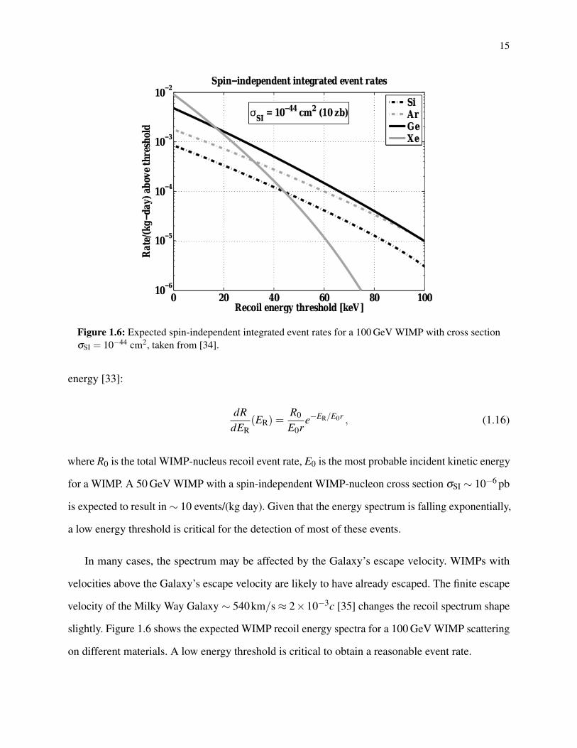
1.6 Expected spin-independent integrated event rates for a 100 GeV WIMP with cross

section σSI = 10−44 cm2. . . . . . . . . . . . . . . . . . . . . . . . . . . . . . . . 15

2.1 The energy spectrum for neutrons produced with (α,n) reactions in the cavern

rock compared to those induced by muon interactions in the rock with and without

shielding. . . . . . . . . . . . . . . . . . . . . . . . . . . . . . . . . . . . . . . . 22

2.2 The total muon flux measured for the various underground laboratories. . . . . . . 23

2.3 The differential energy spectrum for muon-induced neutrons at the various under-

ground laboratories. . . . . . . . . . . . . . . . . . . . . . . . . . . . . . . . . . . 24

3.1 The profile drawing of the Neutron Multiplicity Meter (NMM). . . . . . . . . . . . 30

x

4.1 The previously tuned detector response of 252Cf neutron calibration in Monte Carlo

with Geant4.9.4.p04 and the Monte Carlo detector response based on the same

parameters with Geant4.9.5.p01. . . . . . . . . . . . . . . . . . . . . . . . . . . . 39

4.2 The comparison of individual gamma emission spectra of gadolinium neutron

captures from Geant4 simulations and measurements. . . . . . . . . . . . . . . . . 41

4.3 Fit of muon pulse height spectrum in MC with the measured muon pulse height

spectrum from low-gain data set for tuning the low-gain energy scale factor in MC

offline processor. . . . . . . . . . . . . . . . . . . . . . . . . . . . . . . . . . . . 44

4.4 Fit of muon pulse height spectrum in MC with the measured muon pulse height

spectrum from high-gain data set for tuning the high-gain energy scale factor in MC

offline processor. . . . . . . . . . . . . . . . . . . . . . . . . . . . . . . . . . . . 45

4.5 Fit of the PMT asymmetry distribution from 252Cf neutron simulation with that

from 252Cf calibration run during the time of low PMT gain for the south tank to

tune the East-West Adjustment on PMT energy factors. . . . . . . . . . . . . . . . 49


from 252Cf calibration run during the time of low PMT gain for the north tank to



from 252Cf calibration run during the time of high PMT gain for the south tank to



from 252Cf calibration run during the time of high PMT gain for the north tank to



from 252Cf calibration run during the time of low PMT gain for tuning the smearing

parameter s1. . . . . . . . . . . . . . . . . . . . . . . . . . . . . . . . . . . . . . 53

xi


from 252Cf calibration run during the time of high PMT gain for tuning the smearing

parameter s1. . . . . . . . . . . . . . . . . . . . . . . . . . . . . . . . . . . . . . 54

4.11 The comparison of 252Cf neutron pulse height spectra from simulations with tuned

PMT energy scale and smearing parameters in this work and the pulse height spectra

measured in 252Cf neutron data. . . . . . . . . . . . . . . . . . . . . . . . . . . . 55

4.12 Primary muons in the comprehensive simulation. On the top is the energy spectrum

of the primary muons used in this simulation. . . . . . . . . . . . . . . . . . . . . 59

4.13 The difference in time between a pulse and the MC truth “event” taking place right

before the pulse time. . . . . . . . . . . . . . . . . . . . . . . . . . . . . . . . . . 62

4.14 Pulse multiplicity spectra of the events in different types based on MC truth. . . . . 65

4.15 Pulse spectra of the maximum pulse in each event for different event types. . . . . 67

4.16 Pulse time distributions of neutron capture pulses and muon pulses in different

types of events. . . . . . . . . . . . . . . . . . . . . . . . . . . . . . . . . . . . . 69

4.17 Efficiencies of muon cut for neutron capture events with low PMT gain as a function

of the cut pulse height. . . . . . . . . . . . . . . . . . . . . . . . . . . . . . . . . 72

4.18 Efficiencies of muon cut for neutron capture events with high PMT gain as a

function of the cut pulse height. . . . . . . . . . . . . . . . . . . . . . . . . . . . 73

4.19 Muon pulse spectrum from the events of muons accompanied by neutron captures. 75

4.20 Multiplicity distributions of the events selected for the fast neutron search in the

comprehensive muon simulation. . . . . . . . . . . . . . . . . . . . . . . . . . . . 78

4.21 Muon-induced neutron flux through three surfaces in the comprehensive muon

simulation. . . . . . . . . . . . . . . . . . . . . . . . . . . . . . . . . . . . . . . 81

4.22 Primary neutron energy spectrum of the accepted events, normalized with tank top

surface area and MC live time. . . . . . . . . . . . . . . . . . . . . . . . . . . . . 82

4.23 2-dimensioanl histograms of event multiplicity vs. primary neutron energy. . . . . 84

xii

4.24 The multiplicity distributions of the accepted events, split into the events of real

high-energy neutrons and the events of neutron bundles, with the overall distribution

plotted together. . . . . . . . . . . . . . . . . . . . . . . . . . . . . . . . . . . . . 85

5.1 Comparison of background gammas and high-energy neutrons in event rate with

respect to multiplicity. . . . . . . . . . . . . . . . . . . . . . . . . . . . . . . . . 89

5.2 Comparison of the pulse spectra of neutron captures and background gammas. . . . 91

5.3 Distribution of “pulse-height likelihood” estimator L≡ nn+g for the multiplicity 5

events from the 1st fast neutron search data. . . . . . . . . . . . . . . . . . . . . . 93

5.4 Representation of neutron likelihood in log-likelihood ratio (LLR) log10(n

g

)for the

multiplicity-5 candidate events in the 1st fast neutron search data. . . . . . . . . . 95

5.5 LLR component distribution of multiplicity 5 for each combination of neutron

captures and gamma pulses. . . . . . . . . . . . . . . . . . . . . . . . . . . . . . 97

5.6 An example of mis-coincident muon event with afterpulsing, shown with waveforms

in the four PMT channels. . . . . . . . . . . . . . . . . . . . . . . . . . . . . . . 100

5.7 An example of an electronic noise event, shown with waveforms in the four PMT

channels. . . . . . . . . . . . . . . . . . . . . . . . . . . . . . . . . . . . . . . . 103

5.8 The scatter plots of pulse integral to amplitude ratio (IAR) vs pulse height of the

1st fast neutron search data and the low-gain run of 252Cf calibration. . . . . . . . . 104


2nd fast neutron search data and the high-gain run of 252Cf calibration. . . . . . . . 105


3rd fast neutron search data and the high-gain run of 252Cf calibration. . . . . . . . 106

5.11 The histograms of pulse integral to amplitude ratio (IAR) for the 1st fast neutron

search data and the low-gain run of 252Cf calibration. . . . . . . . . . . . . . . . . 107

5.12 The histograms of pulse integral to amplitude ratio (IAR) for the 2nd fast neutron

search data and the high-gain run of 252Cf calibration. . . . . . . . . . . . . . . . . 108

xiii

5.13 The histograms of pulse integral to amplitude ratio (IAR) for the 3rd fast neutron

search data and the high-gain run of 252Cf calibration. . . . . . . . . . . . . . . . . 109

5.14 Scatter plot of the IAR against multiplicity for the events of multiplicity 9 or greater

having passed the muon rejection cut from all the three fast neutron searches. . . . 110

5.15 The efficiency of the data quality cut of IAR < 0.18, defined as the acceptance

fraction for good 252Cf calibration events. . . . . . . . . . . . . . . . . . . . . . . 112

5.16 Least-squares fit of the LLR distribution for the multiplicity 5 events in the 1st fast

neutron search data. . . . . . . . . . . . . . . . . . . . . . . . . . . . . . . . . . . 116











5.22 Least-squares fit of the LLR distribution for the multiplicity 6 events in the 2nd fast








xiv

5.26 Least-squares fit of the LLR distribution for the multiplicity 10 events in the 2nd

fast neutron search data. . . . . . . . . . . . . . . . . . . . . . . . . . . . . . . . 126

5.27 Least-squares fit of the LLR distribution for the multiplicity 5 events in the 3rd fast










5.32 Least-squares fit of the LLR distribution for the multiplicity 10 events in the 3rd


5.33 The LLR distribution of two data groups with multiplicity greater than 10 in 3rd


5.34 Multiplicity spectrum of the 1st fast neutron search data, compared with the multi-

plicity spectrum of the low-PMT-gain MC. . . . . . . . . . . . . . . . . . . . . . . 138

5.35 Multiplicity spectrum of the 2nd fast neutron search data, compared with the

multiplicity spectrum of the high-PMT-gain MC. . . . . . . . . . . . . . . . . . . 139

5.36 Multiplicity spectrum of the 3rd fast neutron search data, compared with the multi-

plicity spectrum of the high-PMT-gain MC. . . . . . . . . . . . . . . . . . . . . . 140

5.37 Multiplicity spectrum of the combined fast neutron search (FNS) data, compared

with the MC multiplicity spectrum. . . . . . . . . . . . . . . . . . . . . . . . . . . 143

6.1 Conceptual design of the SuperCDMS SNOLAB cryogenic and shielding system. . 149

6.2 Schematic graphs for the layout of the active neutron veto modules. . . . . . . . . 152

6.3 Neutron capture times in the active neutron veto with different boron concentrations.153

xv

6.4 Estimated neutron tagging efficiency, plotted together with capture time, both as

functions of boron concentration. . . . . . . . . . . . . . . . . . . . . . . . . . . . 154

6.5 Veto efficiency for tagging single-scatter neutron-induced iZIP events as a function

of threshold energy in keVee, for veto time window 10 µs, 30 µs, 100 µs, and 300 µs. 156

6.6 The photographs of the quarter-scale neutron-veto prototype. . . . . . . . . . . . . 158

6.7 Screenshots of a 3D visualization for the veto prototype geometry. . . . . . . . . . 159

6.8 The 9 locations of radioactive sources for calibration. . . . . . . . . . . . . . . . . 160

6.9 Energy spectra for a Monte Carlo simulation of the veto prototype exposed with

137Cs at three different locations. . . . . . . . . . . . . . . . . . . . . . . . . . . . 162

6.10 The left column shows the fraction of PE response of individual channels over the

total PE. The right column shows channel number vs the PE fraction, with the color

representing event rate. . . . . . . . . . . . . . . . . . . . . . . . . . . . . . . . . 163

6.11 The measured spectrum of 137Cs compared to a Geant4 137Cs spectrum smeared

using parameters derived from 137Cs and SiPM response. . . . . . . . . . . . . . . 164

6.12 The measured energy spectrum for data collected without any radioactive source

present. . . . . . . . . . . . . . . . . . . . . . . . . . . . . . . . . . . . . . . . . 165

xvi

List of Tables

4.1 Summary of best-fit values of energy scales and smearing parameters in the MC

offline processor. The values of overall energy scale result from the fits shown

in Figure 4.3 and 4.4. The East-West Adjustment is the value added to the east

PMT and subtracted from the west PMT of the best fit energy scale factor for a

PMT gain setting, to fine-tune the energy scale factors for the single PMTs. The

fits of East-West Adjustment are shown in Figure 4.5, 4.6, 4.7, and 4.8. Smearing

paremeters s1 is defined with Eq. (4.2) and the fits for the values are shown in

Figure 4.9 and 4.10. . . . . . . . . . . . . . . . . . . . . . . . . . . . . . . . . . . 56

4.2 Event numbers in each MC event type with each selection requirement found in the

comprehensive muon simulation with 138.8 days of live time. . . . . . . . . . . . . 77

xvii

Chapter 1

Dark Matter

There is compelling evidence for the existence of dark matter from astronomical and cosmological

observations. In this chater, I will briefly present modern cosmology and introduce the evidence

for dark matter, following [1, 2]. In general, I will take the convention of natural units in which the

speed of light is set to one (c = 1). I then discuss the most important dark matter candidate, the

Weakly Interacting Massive Particle (WIMP), and direct detection experiments.

1.1 The Standard Cosmology and the Dark Matter Problem

Cosmology was an ancient and mysterious topic, but only became a real discipline of science

after Einstein’s discovery of general relativity in the early 20th century. General relativity describes

gravitation as a geometric property of spacetime–the curvature, which is directly related to the

energy and momentum of the content of the universe, e.g. matter and radiation. The relation is

specified by Einstein’s equation

Gµν = 8πGTµν , (1.1)

where Gµν is the Einstein tensor representing spacetime curvature, G is Newton’s constant, and Tµν

is the energy-momentum tensor for all fields.

1

2

Besides Einstein’s equation, modern cosmology is based on a fundamental idea known as the

cosmological principle–the universe is homogeneous and isotropic on large scales. The cosmo-

logical principle is not only a hypothesis for simplifying discussions but also supported by many

astronomical observations. The early observation of the cosmic microwave background (CMB) by

COBE found that the anisotropy of the early universe at the time of recombination of protons and

eletrons is only ∼ 10−5.

In the 1920s, Hubble found that the redshifts of celestial objects were proportional to the

distances of the objects away from Earth. The redshift was interpreted as the linear expansion of the

velocity of the objects. This relationship is known as Hubble’s law

v = H0D , (1.2)

where v is the velocity of the object, D is its distance from Earth, and H0 is called the Hubble

constant. Hubble’s law implies that the universe expands uniformly everywhere as time evolves.

We can imagine a frame with comoving coordinates, in which the comoving distance between two

points in space remains constant. However, the physical distance is proportional to a scale factor,

a(t), and the physical distance does evolve with time. To quantify the change in the scale factor, it

is useful to define the Hubble rate

H(t) :=da/dt

a≡ a

a, (1.3)

which measures how rapidly the scale factor changes. The Hubble constant is nothing but the present

value of Hubble rate, H0 = H(t0).

The smooth, expanding universe may be described by the Robertson-Walker (RW) metric

ds2 =−dt2 +a2(t)

[dr2

1− kr2 + r2(dθ2 + sin2

θdφ2)

], (1.4)

3

where t,r,θ ,φ are comoving coordinates. The parameter k determines the curvature of the space:

k =+1 for a spherical, or closed, universe, k = 0 for a flat universe, and k =−1 for a hyperbolic,

or open, universe.

The energy-momentum tensor Tµν on the right-hand side of Einstein’s equation is made of

energy density ρ and pressure p in the universe. With the RW metric, the solution of Einstein’s

equation leads to the two independent Friedmann equations:

H2(t)≡(

aa

)2

=8πG

3

[ρ(t)+

ρcr−ρ0

a2(t)

], (1.5)

and

aa=−4πG

3

(ρ(t)+3p(t)

), (1.6)

where ρ0 is the present value of energy density. The critical density

ρcr ≡3H2

08πG

. (1.7)

The flat universe is one in which the present energy density is equal to the critical density. If the

energy density is higher than the critical density, then the universe is closed; if the energy density is

lower than this value, then the universe is open. There is persuasive observational evidence, e.g. the

anisotropy spectrum of the CMB measured by Planck [3], that stronly supports the flatness of the

universe. With an equation of state p = ωρ (constant ω = 1/3 for radiation, and ω = 0 for matter),

the scale factor evolving over time is then solved from the Friedmann equations,

a ∝ t1/2 (for radiation);

a ∝ t2/3 (for matter).(1.8)

Besides, accoring to the properties of Tµν for radiation and matter, the relationship between energy

4

density and the scale factor can be found as

ρ ∼a−4 (for radiation);

ρ ∼a−3 (for matter).(1.9)

At early times, the scale factor must have been very small, and the energy density very high. In

the standard cosmology, we believe that the universe began from the earliest known periods with a

state of very high density and high temperature, and expanded over time. At early times, the energy

in the universe was dominated by radiation, and the scale factor evolved as a−4. As the universe

expanded, the energy density and temperature dropped, and the density of radiation dropped faster

than that of matter. At later times, nonrelativistic matter dominates the content of energy density,

and the universe then expanded as t2/3. Then at more recent times, another form of energy, known

as dark energy, becomes dominant, making the expansion of the universe accelerate. I will ignore

dark energy for a while until completing the discussion on the evidence of dark matter.

When the universe was much hotter and denser with the temperature at the order of MeV/kB

at the earliest times, there were no neutral atoms or even nuclei. As the universe cooled below the

binding energies of typical nuclei, light elements began to form. This process is known as Big Bang

Nucleosynthesis (BBN). The standard cosmology predicts how the density and temperature dropped

over the early times, and therefore can give precise predictions on the light element abundances

through BBN. Figure 1.1 shows the predictions of BBN and the astronomical measurements of

abundances of four light elements [4]. The measurements are consistent with the predictions, and

provide another confirmation of the standard cosmology. In addition, BBN provides a way of

measuring the baryon density, which is the combined proton plus neutron density, in the universe.

In particular, the measurement of deuterium pins down the baryon density accurately to only ∼ 4%

of the critical density. But the the total energy density has to be the critical energy for a flat universe,

which is strongly supported by many observations. This implies the existence of nonbaryonic matter

in the universe, or known as dark matter.

5

Figure 1.1: Constraint on the baryon density from Big Bang Nucleosynthesis, taken from [4]. Coloredbands show the predictions for four light isotopes–4He, deuterium, 3He, and lithium. Boxes (arrows)show the measured ranges (limits). Fixed by measurements of primordial deuterium, the cyan verticalband shows the baryon density is estimated to be ∼ 4×10−31 gcm−3, i.e. ∼ 4% of critical density.

6

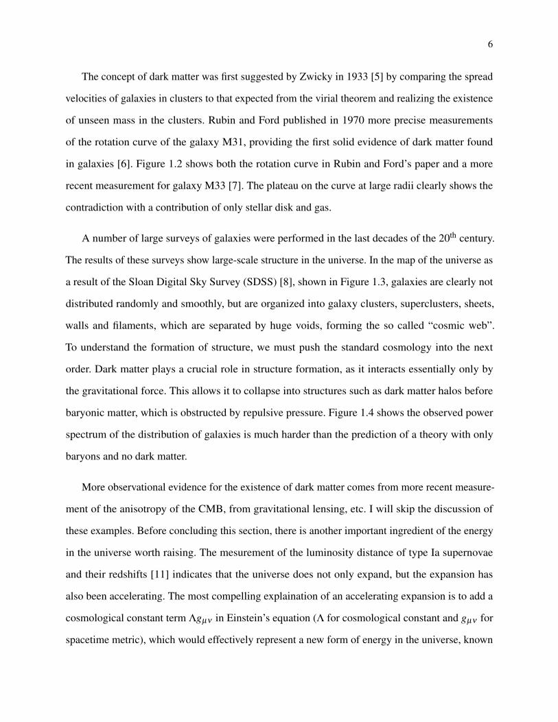
The concept of dark matter was first suggested by Zwicky in 1933 [5] by comparing the spread

velocities of galaxies in clusters to that expected from the virial theorem and realizing the existence

of unseen mass in the clusters. Rubin and Ford published in 1970 more precise measurements

of the rotation curve of the galaxy M31, providing the first solid evidence of dark matter found

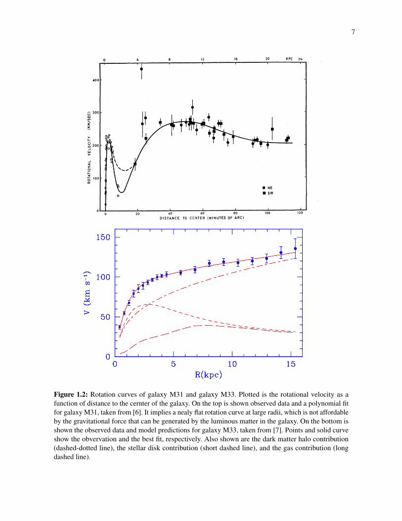
in galaxies [6]. Figure 1.2 shows both the rotation curve in Rubin and Ford’s paper and a more

recent measurement for galaxy M33 [7]. The plateau on the curve at large radii clearly shows the

contradiction with a contribution of only stellar disk and gas.

A number of large surveys of galaxies were performed in the last decades of the 20th century.

The results of these surveys show large-scale structure in the universe. In the map of the universe as

a result of the Sloan Digital Sky Survey (SDSS) [8], shown in Figure 1.3, galaxies are clearly not

distributed randomly and smoothly, but are organized into galaxy clusters, superclusters, sheets,

walls and filaments, which are separated by huge voids, forming the so called “cosmic web”.

To understand the formation of structure, we must push the standard cosmology into the next

order. Dark matter plays a crucial role in structure formation, as it interacts essentially only by

the gravitational force. This allows it to collapse into structures such as dark matter halos before

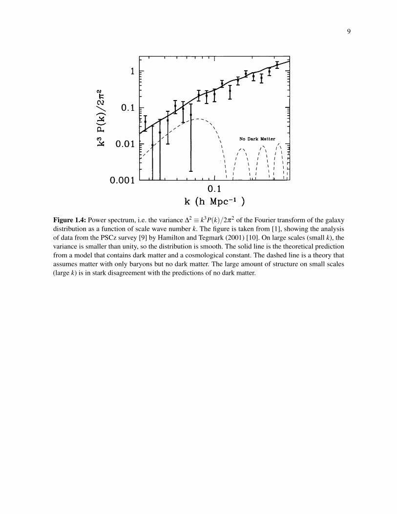
baryonic matter, which is obstructed by repulsive pressure. Figure 1.4 shows the observed power

spectrum of the distribution of galaxies is much harder than the prediction of a theory with only

baryons and no dark matter.

More observational evidence for the existence of dark matter comes from more recent measure-

ment of the anisotropy of the CMB, from gravitational lensing, etc. I will skip the discussion of

these examples. Before concluding this section, there is another important ingredient of the energy

in the universe worth raising. The mesurement of the luminosity distance of type Ia supernovae

and their redshifts [11] indicates that the universe does not only expand, but the expansion has

also been accelerating. The most compelling explaination of an accelerating expansion is to add a

cosmological constant term Λgµν in Einstein’s equation (Λ for cosmological constant and gµν for

spacetime metric), which would effectively represent a new form of energy in the universe, known

7

Figure 1.2: Rotation curves of galaxy M31 and galaxy M33. Plotted is the rotational velocity as afunction of distance to the cernter of the galaxy. On the top is shown observed data and a polynomial fitfor galaxy M31, taken from [6]. It implies a nealy flat rotation curve at large radii, which is not affordableby the gravitational force that can be generated by the luminous matter in the galaxy. On the bottom isshown the observed data and model predictions for galaxy M33, taken from [7]. Points and solid curveshow the obvervation and the best fit, respectively. Also shown are the dark matter halo contribution(dashed-dotted line), the stellar disk contribution (short dashed line), and the gas contribution (longdashed line).

8

Figure 1.3: A slice through the Sloan Digital Sky Survey 3-demensional map of the distribution ofgalaxies with the Earth at the center.

as dark energy, or vacuum energy. Dark energy has an equation of state p =−ρ , with which the

second Friedmann equation Eq. (1.6) results in a positive a. The density of vacuum energy remains

constant no matter how the scale factor a changes. Thus as the universe expands, and radiation and

matter become diluted enough, the dark energy density starts to dominate the universe, and drive

the expansion to accelerate. In addition, the baryonic, ordinary matter only contributes at most 5%

of the critical density, as mentioned earlier. But, recent estimate of dark matter density takes 24%

of the critical density. Therefore, in considering the “budgetary shortall”, dark energy is needed as

∼ 71% of the critical energy to ensure the universe is flat.

At present, the most compelling cosmology model is known as the ΛCDM model: a flat universe

with a non-zero cosmological constant Λ and Cold (non-relativistic) Dark Matter (CDM). The

dominant form of energy density, dark energy, is not well understood yet. And although there is

a lot of evidence for dark matter on the side of cosmology and astronomy, we have not directly

detected dark matter, and confirmed nothing about what dark matter is in the particle physics sense.

9

Figure 1.4: Power spectrum, i.e. the variance ∆2 ≡ k3P(k)/2π2 of the Fourier transform of the galaxydistribution as a function of scale wave number k. The figure is taken from [1], showing the analysisof data from the PSCz survey [9] by Hamilton and Tegmark (2001) [10]. On large scales (small k), thevariance is smaller than unity, so the distribution is smooth. The solid line is the theoretical predictionfrom a model that contains dark matter and a cosmological constant. The dashed line is a theory thatassumes matter with only baryons but no dark matter. The large amount of structure on small scales(large k) is in stark disagreement with the predictions of no dark matter.

10

1.2 Weakly Interacting Massive Particles

There are many candidate particles proposed in theory, including the axion [12], Kaluza-Klein

particle [13], gravitino [14], etc. Currently the most compelling theory is a general class called

Weakly Interacting Massive Particles [15], or WIMPs, which both satisfies the cosmological criteria

of being cold, non-baryonic relic and meets the role in new physics for solving the hierarchy

problem [16]. Most direct dark matter detection experiments are designed to discover WIMPs.

Figure 1.5: Comoving number density of WIMP dark matter in the early Universe, taken from [17].The solid curve is the equilibrium abundance, while the dashed curves are the actual WIMP abundanceresulting from three different values of thermal averaged pair annihilation cross section of WIMPs.Larger values of the annihilation cross section would leave smaller amounts of WIMP relics today.

In the generic WIMP scenario, two heavy particles (WIMPs) can annihilate to produce two light

(or massless) particles, which are assumed to be very tighly coupled to the cosmic plasma. This

process is reversible when the temperature is high enough for the process to produce the mass of the

11

WIMP, and the WIMPs are in equilibrium with the cosmic plasma. Its abundance is suppressed as

e−m/T as temperature drops. When the temperature of the universe further drops below the mass

of WIMP, they become so rare due to this suppression that they are not able to find each other fast

enough to maintain the equilibrium abundance. In fact, WIMP particles begins to freeze out from

the equilibrium, and its comoving density then becomes invariant. For non-relativistic particles, the

dark matter density parameter when freeze-out occurs is [18]

ΩDMh2 ≈ 3×10−27

< σAv >cm3/s , (1.10)

where < σAv > is the thermal-averaged pair annihilation cross section of WIMPs,

h≡H0/(100kmsec−1 Mpc) is the dimensionless Hubble parameter, and ΩDM is the fractional dark

matter density. It is conventional to use the product as the parameter for dark matter density. The

dark matter density is independent of the mass of the WIMP. Figure 1.5 shows the comoving number

density of the dark matter in equilibrium drops exponentially as the temperature decreases; with

three different annihilation cross sections, WIMP dark matter would freeze out from the equilibrium

with different densities [17]. A larger dark matter annihilation cross section means that the WIMPs

stay in equilibrium longer, and leave the density of the relic today lower.

New physics beyond the Standard Model is needed to solve the hierarchy problem in particle

physics. If a new particle interacting with the electroweak scale exists, its annihilation cross section

can be estimated to be < σAv >∼ α2(100GeV)−2 ∼ 10−25cm3 s−1, for α ∼ 10−2 [18]. It is close to

the value needed to leave the right amount of dark matter in the unvierse. This striking coincidence

has brought great motivation to assume the lightest stable particle at the electroweak scale to be the

dark matter. The WIMP models have been studied with extensive theoretical work, and have led to

a tremendous experimental effort in last two decades to detect these WIMPs [19–27].

12

1.3 Direct Dark Matter Detection

WIMP dark matter can potentially be detected by three complementary methods. WIMPs may

be produced at high-energy accelerators such as the Large Hadron Collider (LHC) and detected

indirectly by identifying the signal of missing energy [28]. Relic WIMPs may be detected indirectly

when they gather more densely in massive celestial objects, increasing their annihilation rate enough

and producing detectable signals [29]. Many indirect signals may have alternate astrophysical

explanations, making these indirect detections ambiguous.

Relic WIMPs may be directly detected when they recoil off nuclei in terrestial detectors [30,

31]. Direct dark matter detection is the most compelling method to test the WIMP hypothesis as

compared with the other two methods, since it may find the most unambiguous signals. I will present

in this section the generic characteristics of WIMP signals in direct detection, and briefly introduce

implementations of these experiments, primarily following [32].

1.3.1 Spin-independent and Spin-dependent Cross Sections

Using Fermi’s Golden Rule, the differential WIMP-nucleon cross section can be found dependent

on the zero-momentum cross section independent of the momentum transfer, σ0WN, and the form

factor F2(q):

dσWN(q)dq2 =

1πv2 |M|

2 =σ0WNF2(q)

4µ2Av2 . (1.11)

Here, v is the velocity of the WIMP in the lab frame, and the WIMP-nucleon reduced mass

µA ≡MχMA/(Mχ +MA) in terms of the WIMP mass Mχ and the mass MA of a target nucleus of

atomic mass A. The zero-momentum cross section for a non-relativistic WIMP of arbitrary spin

13

may be further written in terms of a spin-independent and a spin-dependent term:

σ0WN =4µ2

Aπ

[Z fp +(A−Z) fn

]2+

32G2Fµ2

Aπ

J+1J

(ap < Sp >+an < Sn >

)2. (1.12)

Here the two terms describe spin-independent and spin-dependent WIMP-nucleus cross section. fp

and fn (ap and an) are effective spin-independent (spin-dependent) couplings of the WIMP to the

proton and neutrons, respectively. These couplings and the WIMP mass Mχ are the parameters that

contain all the information of the particle physics models; the other parameters describe the target

nuclei, i.e. the atomic number Z, mass number A, total nuclear spin J, and the expectation values of

the proton and neutron spins within the nucleus < Sp,n >=< N|Sp,n|N >. For many models, fp ≈ fn,

then the atomic number Z cancels in the spin-independent WIMP-nucleus cross section

σ0WN,SI ≈4µ2

Aπ

f 2p A2 = σSI

µ2A

µ2n

A2 , (1.13)

where µn is the reduced mass of the WIMP-nucleon system. In the last part of the equation, the

spin-independent WIMP-nucleus cross section is rewritten by defining the spin-independent cross

section of a WIMP interacting on a single nucleon

σSI ≡4µ2

n f 2n

π. (1.14)

This spin-independent WIMP-nucleon cross section σSI can be used to compare among different

experiments and compare to models. A given model predicts a range in σSI and Mχ parameter space;

experiments quote limits on σSI as functions of Mχ as their results, or would measure values of

σSI and Mχ if making a discovery. The dependence on A2 in Eq. (1.13) suggests the advantage of

using target materials with heavy elements. For the spin-dependent interactions, contributions from

proton and neutron couplings often cancel. The detection limits on the spin-dependent cross section

should be quoted separately for neutrons and protons, each under the assumption that the other

interaction is negligible. Also, the spin-dependent contributions of nucleons with opposite spins

14

cancel, so that the coherent spin-dependent cross section depends on the net spin of the nucleus.

Nuclei with even numbers of protons (neutrons) have nearly no net proton (neutron) spins and

hence no sensitivity to spin-dependent interactions on protons (neutrons). Argon is insensitive to

spin-dependent interactions because of its even numbers of protons and neutrons for all significant

isotopes. Many other materials used as WIMP targets, such as Ge, Si, Xe, have even numbers

of protons, therefore are insensitive to spin-dependent interactions on protons. And only some

isotopes of these targets, which reults in a fraction of the detector’s active mass, have sensitivity

to spin-dependent interactions on neutrons. Typically, the target materials that are sensitive to

spin-dependent interactions often result in worse backgrounds or background rejection and lower

sensitivity to spin-independent interactions. Most models are more accessible experimentally via

their spin-independent interactions than by their spin-dependent interaction.

1.3.2 The WIMP Recoil Energy Spectrum

Based on simple consideration of conservation of momentum and energy, the maximum recoil

energy max(ER) for an elastic collision of a WIMP with kinetic energy Eχ on a nucleus satisfies

max(ER)

Eχ

=4MχMA

(Mχ +MA)2 =4µ2

AMχMA

≡ r . (1.15)

The recoil energy ER of each WIMP scatter would distribute randomly from zero to the maximum

recoil energy max(ER), as the recoil angle varies. Here let’s call this ratio r for convenience. The

mean recoil energy is one half this amount. In typical models, a 100 GeV WIMP with a kinetic

energy of ∼ 40keV would deposit ∼ 20keV in the lattice by recoiling off a 67 GeV germanium

nucleus. By including the distribution of recoil energies with different max(ER) values, the general

form for the recoil energy spectrum can be written into a falling exponential as a function of recoil

15

Figure 1.6: Expected spin-independent integrated event rates for a 100 GeV WIMP with cross sectionσSI = 10−44 cm2, taken from [34].

energy [33]:

dRdER

(ER) =R0

E0re−ER/E0r , (1.16)

where R0 is the total WIMP-nucleus recoil event rate, E0 is the most probable incident kinetic energy

for a WIMP. A 50 GeV WIMP with a spin-independent WIMP-nucleon cross section σSI ∼ 10−6 pb

is expected to result in∼ 10 events/(kg day). Given that the energy spectrum is falling exponentially,

a low energy threshold is critical for the detection of most of these events.

In many cases, the spectrum may be affected by the Galaxy’s escape velocity. WIMPs with

velocities above the Galaxy’s escape velocity are likely to have already escaped. The finite escape

velocity of the Milky Way Galaxy ∼ 540km/s≈ 2×10−3c [35] changes the recoil spectrum shape

slightly. Figure 1.6 shows the expected WIMP recoil energy spectra for a 100 GeV WIMP scattering

on different materials. A low energy threshold is critical to obtain a reasonable event rate.

16

1.3.3 Direct Detection Technologies

There are primarily three classes of technologies in use for WIMP direct detection experiments,

distinguished with the way of collecting the deposited WIMP recoil energy, i.e. collecting energy

via charge, light, or phonons/heat. Two types of target materials are mostly in use. Cryogenic semi-

conductor crystals were developed earlier, but the detectors using noble elements have demonstrated

great advantages and have now published the strongest limits on spin-independent WIMP-nucleon

cross sections above 10 GeV WIMP mass [36, 37].

Detectors using noble elements, with either single-phase (liquid) or dual-phase, generate signals

by collecting scintillation light. A nuclear-recoil event in a noble liquid creates dimers in singlet

states or triplet states, which de-excite in different characteristic times with emission of scintilla-

tion light. The nuclear recoils (induced by WIMPs or neutrons) and electron recoils (induced by

gamma-rays or electrons) differ in the fraction of singlet states and triplet states, therefore result

in dramatically different pulse shapes. With this property, noble liquid detectors reject gamma

backgrounds with the technique called pulse shape discrimination (PSD). These experiments are

usually designed with a fiducial volume, within which the events are accepted as candidates. The

detector mass outside the fiducial volume is used as self-shielding against surface backgrounds. The

examples of this type of experiment include MiniCLEAN [19, 20] and DEAP-3600 [21]. Some

noble liquid detectors also apply an electrical field and collect both scintillation light and ionization

charge. These exepriments include LUX [22], XENON100 [23], Darkside [24].

Detectors using cryogenic semiconductors have excellent energy resolution to help identify

the sources of the backgrounds from natural radioactivity in the experimental apparatus and envi-

ronment. Many of these detectors, such as SuperCDMS [25] and EDELWEISS [26], collect both

ionization charge and phonons. The ratio of energy from these two signal channels provide excellent

discrimination against electron recoils. The CoGeNT exepriment [27] uses p-type point contact

(PPC) detectors with ionization charge readout only.

17

Although most of these experiments have demonstrated excellent discrimination between nuclear

recoils and electron recoils, single-scattered neutron events cannot be distinguished from WIMP

recoils. In the next chapter, I will further discuss neutron backgrounds and the strategies of dealing

with neutron backgrounds for direct dark matter detection.

Chapter 2

Neutron Backgrounds

Neutrons can scatter off nuclei just like WIMPs do, resulting in a mimic of WIMP detection signals.

The neutron-nucleus elastic scattering cross section is of course much higher than the expected

WIMP-nucleus scattering cross section, so a neutron interaction with a detector would have a much

higher chance to induce multiple scatters in the detector mass, which is a feature used to reject

neutron background events. However, when neutrons produced single nuclear recoils, the events

would be detected as truly indistinguishable background events, leaving the experimental results

ambiguous. Therefore, it is crucial to accurately characterize and minimize neutron backgrounds.

Due to intrinsic contamination with 238U, 235U, and 232Th in materials of the detector, shielding,

and in lab cavern rock, radiogenic neutrons with kinetic energies up to several MeV are produced

with (α,n) reactions and spontaneous fission (SF). See e.g. [38]. The radiogenic neutron back-

grounds are described in Section 2.1. In addition, cosmogenic neutrons with energies extending

to a few GeV are generated with the interactions of cosmic-ray muons with the rock surrounding

the underground laboratory. As the overburden above the underground site increases, the flux of

muons drops, but the average energy of muons increases. This makes the flux and energy spectrum

of cosmogenic neutrons dependent on laboratory’s depth. The cosmogenic neutron backgrounds are

described in Section 2.2.

18

19

2.1 Radiogenic Neutrons

Radiogenic neutron backgrounds for direct WIMP search experiments are produced by (α,n)

reactions with the α particles emitted primarily from uranium and thorium radioactive isotope

decays in the materials surrounding or constituting the detector, and also produced by spontaneous

fission of uranium and thorium. Usually, the (α,n)-produced neutrons dominate the total neutron-

induced background for an underground experiment.

The general strategy to minimize radiogenic neutron background for underground experiments

is to shield the detector with neutron moderators, which are hydrogen-rich materials. The neutron

moderators most often used as shieding materials for dark matter experiments include water, high-

density polyethylene (HDPE). As the hydrogen nucleus (a proton) has a mass very close to the mass

of neutron, the elastic collision of a neutron onto a nearly static proton is very effective at reducing

the speed of the incoming neutron. With a proper shield, the radiogenic background neutrons can be

moderated to very low energies so that they are evantually captured in shieding materials, or reach

the detector but are not energetic enough to induce nuclear recoils above the experiment’s threshold

energy.

Both for appropriately designing the shielding system and for analyzing the WIMP search

data, the neutron induced background in the region of interest (ROI) must be evaluated in Monte

Carlo simulations. Neutrons designated to start in the bulk or on the surface of all the materials

of the detector, or surrounding the detector, need to be properly assigned with emission rates and

energy spectra, which are crucial in determining the total background events in the ROI. Therefore,

the radiogenic neutrons need to be understood very well in terms of their origin, transport, and

interaction with different materials.

The neutron yield of the (α,n) reactions for various elements have been discussed by many

authors [39–42]. The α particles produced from uranium and thorium decays in materials travel

with energies in the MeV range. They interact with the nuclei in a thick target and generate neutrons.

20

The neutron yield is calculated by [41]

Yi =NA

Ai

∫ E0

0

σi(E)Sm

i (E)dE , (2.1)

where E0 is the initial energy of the α particle, Smi is the mass stopping power of element i, Ai is the

atomic mass of element i, and NA is Avogadro’s constant. The neutron yields in the uranium and

thorium decay chains can be determined by summing the individual yields induced by each α in

the decay chain, with the weights based on the branching ratio for each element and the mass ratio

in the host materials. The energy attenuation of the α particles is the dominant process in the host

materials under the thick target hypothesis [43]. Assuming that the incoming α particle flux with

energy E j is invariant until the energy is attenuated to zero, the differential spectra of neutron yield

can be derived as

Yi(En) =Ni ∑j

Φα(E j)∫ E j

0

dσ(Eα ,En)

dEα

dEα

=NA

Ai∑

j

Rα(E j)

Smi (E)

∫ E j

0

dσ(Eα ,En)

dEα

dEα ,

(2.2)

where Ni is the the total number of atoms for the element i in the host material, Φα(E j) is the

incoming α particle flux with specific energy E j, Rα(E j) is the α particle production rate as a

funcion of the energy E j from the uranium or thorium decay chain. The cross sections used in

Eq. (2.2) can either be calculated with simulation code, such as TALYS [44], or obtained from

nuclear data bases, such as ENDF [45], or TENDL [46].

Many dark matter direct detection experiments use the SOURCES code [47] to calculate the

neutron yield of (α,n) reactions. But the software is not open-source, so the lack of accessibility

may prevent it from being easily modified with more and better data, which is strongly needed

for the dark matter detection and the broader low-background counting community. C. Zhang,

D.-M. Mei, and A. Hime performed an independent calculation of the (α,n) neutron yield for

various materials, and developed the Radiogenic Neutron Generator (RNG), a web based generator

21

with data base [43]. The effort comparing the neutron yields and spectra calculated by the two

softwares, and how the difference would result in the detectable neutron background in the dark

matter ROI have been ongoing [48, 49].

2.2 Cosmogenic Neutrons

Direct dark matter detection experiments are placed and run at underground laboratories, as the

overburden provides a natural shield against cosmic-ray muons and their induced particles. The

remaining muons that traverse a detector and its surrounding material, but miss an external veto,

serve as a background themselves. In addition, the interactions of muons with the surrounding

materials and cavern rock can produce fast neutrons and activate radioactivities. The muon-induced

neutrons are particularly important, as they become a source of neutron background in addition to

the radiogenic neutrons. In general, the production rate of muon-induced neutrons at large depths

is 2 to 3 orders of magnitude smaller than that of radiogenic neutrons. The latter typically have

MeV neutron energies, and are hence relatively easy to shield. On the other hand, the cosmogenic

muon-induced neutrons have a very hard energy spectrum, extending to several GeV. The high-

energy muon-induced neutrons can easily penetrate the detector shielding materials. In addition,

they may interact with the high-Z materials, such as lead and copper, which are commonly used

as shielding materials against external gamma-rays, and generate multiple secondary neutrons in

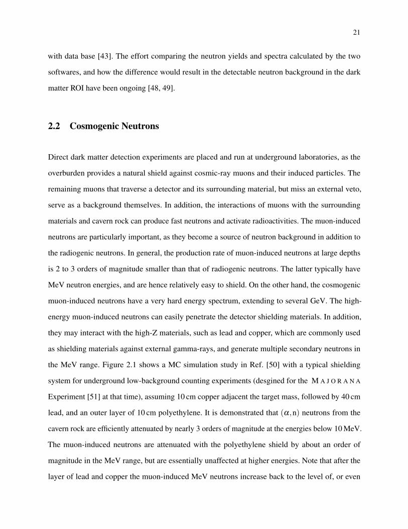
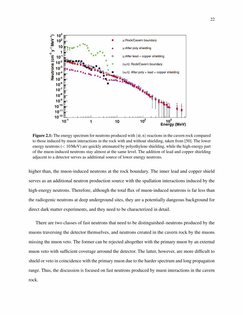
the MeV range. Figure 2.1 shows a MC simulation study in Ref. [50] with a typical shielding

system for underground low-background counting experiments (desgined for the M A J O R A N A

Experiment [51] at that time), assuming 10 cm copper adjacent the target mass, followed by 40 cm

lead, and an outer layer of 10 cm polyethylene. It is demonstrated that (α,n) neutrons from the

cavern rock are efficiently attenuated by nearly 3 orders of magnitude at the energies below 10 MeV.

The muon-induced neutrons are attenuated with the polyethylene shield by about an order of

magnitude in the MeV range, but are essentially unaffected at higher energies. Note that after the

layer of lead and copper the muon-induced MeV neutrons increase back to the level of, or even

22

Figure 2.1: The energy spectrum for neutrons produced with (α,n) reactions in the cavern rock comparedto those induced by muon interactions in the rock with and without shielding, taken from [50]. The lowerenergy neutrons (< 10MeV) are quickly attenuated by polyethylene shielding, while the high-energy partof the muon-induced neutrons stay almost at the same level. The addition of lead and copper shieldingadjacent to a detector serves as additional source of lower energy neutrons.

higher than, the muon-induced neutrons at the rock boundary. The inner lead and copper shield

serves as an additional neutron production source with the spallation interactions induced by the

high-energy neutrons. Therefore, although the total flux of muon-induced neutrons is far less than

the radiogenic neutrons at deep underground sites, they are a potentially dangeous background for

direct dark matter experiments, and they need to be characterized in detail.

There are two classes of fast neutrons that need to be distinguished–neutrons produced by the

muons traversing the detector themselves, and neutrons created in the cavern rock by the muons

missing the muon veto. The former can be rejected altogether with the primary muon by an external

muon veto with sufficient coverage arround the detector. The latter, however, are more difficult to

shield or veto in coincidence with the primary muon due to the harder spectrum and long propagation

range. Thus, the discussion is focused on fast neutrons produced by muon interactions in the cavern

rock.

23

Figure 2.2: The total muon flux measured for the various underground laboratories, taken from [50].The measured data are from [52–55].

The flux of cosmogenic fast neutrons strongly depends on the depth and composition of an

underground laboratory. D.-M. Mei and A. Hime studied with Monte Carlo simulations the site/depth

dependence for neutron yield and the flux of muon-induced neutrons [50]. The total muon flux

has been measured at the various underground sites. Figure 2.2 shows the muon flux and depth

relationship. The total muon flux decreases as the site goes deeper. However, the mean muon energy

increases as the site goes deeper, because with more overburden only harder muons have larger

probabilities to survive, leaving the softer muons already attenuated. The production of muon-

induced neutrons at an underground site depends on both the total muon flux and neutron yield. The

latter is positively related to mean muon energy. Mei and Hime obtained the simulated differential

neutron flux at several sites, shown in Figure 2.3. Based on the differential flux at the various sites,

they privided a convenient parametrization (now known as the Mei-Hime parametrization)

dNdEn

= Aµ

(e−a0En

En+Bµ(Eµ)e−a1En

)+a2E−a3

n , (2.3)

24

Figure 2.3: The differential energy spectrum for muon-induced neutrons at the various undergroundlaboratories, taken from [50]. The bin width is 50 MeV.

25

where Aµ is a normalization constant, a0, a1, a2, and a3 are fitted parameters, En is the neutron

energy, and Bµ(Eµ) is a function of muon energy Eµ in GeV,

Bµ(Eµ) = 0.324−0.641e−0.014Eµ . (2.4)

In the paper, they also provided the fit parameters. The parametrization is valid for En > 10MeV.

In recent years, there has been experimental effort to characterize the cosmogenic muon-induced

neutrons at underground laboratories. The work in Ref. [56] measured the fast neutron flux at

Soudan Mine with liquid scintillator, resulting in 2.3±0.52(sta.)±0.99(sys.)×10−9 cm−2 s−1

for fast neutrons above 20 MeV, in a reasonable agreement with the model prediction discussed

above. In a recent publication [57], an experiment called Muon-Induced Neutron Indirect Detection

EXperiment (MINIDEX) has been run to measure neutrons induced by cosmic-ray muons in selected

high-Z materials. The results from the first round of data have indicated a factor of 3 to 4 excess

on the rate of muon-induced neutrons compared to Geant4 prediction. The neutrons measured by

this experiment are not the same type of events that we are most interested in, since these events

should be easy to tag with a muon veto. However, this experiment provides interesting results in

benchmarking Monte Carlo predictions against data on cosmogenic neutron production.

In order to provide more useful data with which to benchmark simulations, the Neutron Multi-

plicity Meter (NMM) experiment [58] was built and at Soundan Mine. In the following chapters of

this thesis, I will introduce the NMM detector, and present the Monte Carlo study and data analysis

that I have done, in an effort to measure the cosmogenic neutron flux and benchmark neutron

production with the Geant4 Monte Carlo simulations.

Chapter 3

The Neutron Multiplicity Meter at the Soudan

Underground Laboratory

3.1 Motivation

Neutrons in underground laboratories are one of the most challenging backgrounds to direct dark

matter detection experiments, as they cause nuclear recoils in detector mass to mimic WIMP signals.

Proper design and operation of the dark matter experiment and correct analysis of the results rely

on numerical Monte Carlo simulations to predict the background rate due to neutrons. At depths

of 2000 meters of water equivalent (m.w.e.) and below, the neutron-induced background rate is

correlated with the flux of high-energy neutrons (also called fast neutrons) produced by cosmic

ray-muons interacting with cavern rock. The simulation of these processes is uncertain due to the

lack of appropriate measurement of the fast neutron flux in underground laboratories for direct

comparison.

The issue is intensified with neutron spallation processes induced by fast neutrons in high-

Z shielding materials near the detector. To reduce the gamma background for WIMP direction

experiments, high-Z materials such as lead are used to attenuate gammas from ambient U, Th,

etc. While the high-Z materials are effective against gamma rays, the shield itself may become an

26

27

increased neutron source due to the neutron spallation process caused by unvetoed muon-induced

fast neutrons. These neutrons have energies above ∼50 MeV, and thus low enough cross section

on hydrogen that they can easily penetrate the shielding for moderating low-energy neutrons and

reach the high-Z gamma shield. They tend to interact with the high-Z materials and cause spallation

processes, which result in multiple secondary neutrons with energies below 10 MeV. These lower-

energy neutrons, generated inside the neutron moderator, can easily reach the innder dark matter

detector and mimic WIMP signals. The lack of knowledge on the fast neutrons induced spallation

process and the lack of data on the fast neutron flux in underground laboratories together make the

backgrounds due to the muon-induced neutrons a challenging issue for dark matter experiments.

The Neutron Multiplicity Meter (NMM) [58] was proposed and built to pin down the flux

of the muon-induced fast neutrons to about 10% at the Soudan Underground Laboratory, at a

depth of approximate 2000 m.w.e. Utilizing the high thermal-neutron capture cross section of

gadolinium and using water serving both as a neutron moderator and a Cherenkov medium, the

experiment has implemented a neutron multiplicity meter adjecent to a lead target, which is used as

gamma shield in actual dark matter experiments, such as SuperCDMS [25]. When a high-energy

neutron hits the lead target, the neutrons spallation, similar as it takes place in lead shielding of

dark matter experiments, results in multiple neutrons with energies below 10 MeV. Most of theses

neutrons will be thermalized and captured by gadolinium nuclei and result in detectable light. The

multiplicity of the secondary neutrons provides both a distinct signature of the fast neutron event

and an indirect measurement of its initial energy. The data on the NMM not only measures the

flux of the muon-induced high-energy neutrons at the Soudan Underground Laboratory, but also

acquires information about the high-energy neutron spectrum and allow the underlying neutron

production processes in Pb to be measured. Together, the flux and multiplicity distribution will help

to benchmark the simulation codes and shed light on modeling the underlying processes. Being

able to predict cosmogenic neutron background with greater reliability benefits the whole low

background counting community, and helps improve extrapolations for the experiments aiming

to operate in deeper sites, such as SuperCDMS SNOLAB. The successful operation of the NMM

28

at Soudan depth and results of the measurement demonstrates the feasibility of larger detectors

with similar techniques that may be built and run for high-energy neutron benchmarking studies at

greater depths.

3.2 Detection Technique

The main techniques of the Neutron Multiplicity Meter is utilizing the water-Cherenkov effect

induced by the gamma rays from gadolinium neutron-captures to measure the rate of high-energy

neutrons underground and the secondary neutron multiplicity of the spallation induced by the

primary high-energy neutron in a lead target.

High-energy neutrons are difficult to stop. The idea of the design of the experiment is to convert

a high-energy neutron into several secondary neutrons with lower energies. The major part of the

detector is two moderate sized tanks filled with Gd-loaded water atop a lead stack as the detector

target. A high-energy neutron induced by cosmic-ray muon in rock underground will mainly enter

from above, penetrate the water, and cause neutron spallation in the Pb target. The disintegration of

the Pb nucleus will release several neutrons with typical energy below 10 MeV emitted isotropically.

Some of these neutrons leave the lead stack and enter the Gd-loaded water, where they are quickly

moderated and thermalized by the protons in water. These thermal neutrons will travel in water until

they find a gadolinium nucleus, which has a high thermal-neutron capture cross section, and most

will be captured within a characteristic time of ∼10 µs. The resulted excited nuclear state will decay

and emit gamma rays of ∼8 MeV after the capture. Then the consequent electromagnetic cascades

will produce Cherenkov lights, which can be collected by the PMTs immersed in the water.

The captures of the thermal neutrons by the Gd nuclei in water take place as a Poisson process,

and the rate of the captures decays exponentially since the first capture. This behavior makes

advantage to the high-energy neutron detection: the neutrons released simultaneously in burst of

several are spread out in time, and individually captured and counted. The characteristic timing

29

distribution of the neutron captures also provides a unique signature of pulse clustering which allows

tagging of neutron multiplicity events as well as effective rejection of random gamma backgrounds.

The neutrons released via spallation induced by the primary high-energy neutron in Pb carry

typical kinetic energy below 10 MeV. This fact features that the counting of the neutron multiplic-

ity gives a rough indication of the primary neutron energy. Therefore the measured multiplicity

distribution will provide extra information, other than the event rate only, for benchmarking the

generation of the muon-induced neutrons underground, as well as the neutron spallation in Pb.

3.3 Detector Description

The Neutron Multiplicity Meter (NMM) ran and took data at the Soudan Underground Laboratory

at a depth of 1.95 km.w.e. There are dark matter experiments SuperCDMS and CoGeNT at the

Soudan lab sharing the same cavern with the NMM.

3.3.1 Main Components

Figure 3.1 is a cross-sectional view of the NMM. The detector consists of two optically separated

water tanks, each containting 2 tons of water and holding two 20 inch KamLand photomultiplier

tubes (PMTs) [59] with the surfaces immersed in water. Each tank is 96 inches long, 48 inches

wide, and 30 inches high. Both tanks align on their longer sides, creating an essentially 96×96 inch

square area, though there is a small gap between the two tanks due to the longer extents of their

caps. The two water tanks sit atop 16 inches of stacked lead bricks, with a 84×80 inch footprint.

The size of the lead footprint was chosen so the experiment would have a reasonable event rate:

approximately 1 high-energy neutron candidate event per day. The water tanks extend past the lead

stack to better cover the upward spallation neutrons emitted from Pb. The tank size is also motivated

by the need for a high collection efficiency of the neutron-capture gammas: the water tanks need

30

to be large enough to catch most of capture gammas via Compton scattering. There are several

cylindrical tubes embedded under the top layer of Pb stack, allowing calibration sources to be easily

placed underneath each tank. One layer of 2 inch lead bricks are placed on top and three sides of

each tank for background gamma shielding. The south tank is further elevated by an additional layer

of lead bricks to make the gap between the two tanks smaller by letting the cap margins overlay. The

Figure 3.1: The profile drawing of the Neutron Multiplicity Meter (NMM). A stack of 16 inches high,20 tonne lead serves as the target mass, with a footprint of 84 × 80 inches. Atop of the lead stack are twotanks of water, each 2 tons. On top of each water tank, there are two 20 inch KamLand PMTs, 4 in total,with the surfaces immersed in water. Both tanks aligning with the longer side of each other creates anessentially 96 × 96 inch square area, though there is a small gap in between two tanks due to the longerextents of their caps. One layer of 2 inch lead bricks are placed on top and three sides of each tank forbackground gamma shielding. The south tank is further elevated by an additional layer of bead bricks tomake the gap between the two tanks smaller by letting the cap margins overlay.

water is Gd-loaded in forms of Gadolinium Trichloride. The two tanks have different concentrations

of gadolinium: the south tank has 0.3% Gadolinium Trichloride, or effectively 0.2% Gd, and the

north tank 0.7%, effectively 0.4% Gd. This will result in different capture times in the two tanks:

the secondary neutrons are captured faster in the north tank than in the south tank. The water also

31

has approximately 1 ppm of Amino-G Salt, a water soluble wavelength shifter. The acrylic tanks

are lined inside with highly reflective sintered Halon, with a diffuse reflectivity of approximately

94% [60].

3.3.2 Trigger, Electronics, and DAQ

The signal of the detector is based on the PMT collection of the photons emitted via Cherenkov

effect by the Compton scatterd high-speed electrons resulting from neutron-capture gammas. The

detector trigger is designed based on the pulse multiplicity of the event in both tanks. The logical

AND is defined for each tank as both PMTs firing a pulse above a 10 mV threshold within 160 ns

of each other. The 160 ns coincidence time is set so to allow the photons resulting from the same

neutron capture to reach both PMTs: the light may traverse the approximately 2 meter length of

the water tank, and reflect on the order of ten times before hitting a PMT or being absorbed by the

water. The requirement of coincident firing in both PMTs of each tank is set to suppress the false

triggering by electronic noise and background gammas with very low energies. The multiplicity

is defined as the number of logical ORs between the ANDs of the two tanks. Whether there is a

single pair of coincident pulses in one tank, or a pair of coincident pulses in each tank taking place

within 160 ns of each other to form a quadruple coincidence, the coincident pulses are counted

as one in multiplicity. The trigger of an event is set on the total multiplicity within a given time

window, e.g. triggering on multiplicity 5 in 60 µs. It takes advantage of the characteristic timing

distribution of the secondary neutron captures. The captures of the secondary neutrons and their

resulting pulses are clustered in time toward the first one, while the background gamma-induced

pulses spread evenly in time, therefore the setting of trigger on multiplicity for a given time interval

will do a great job discriminating the gamma backgrounds. Once an event is triggered, a 100 µs

pre-trigger window and a 100 µs post-trigger window from the trigger time are recorded. The DAQ

system of the detector, constructed entirely from commercial modules, records digitized waveforms

of each channel (PMT) over the 200 µs window.

32

3.4 Data and Reduction

The digitized waveform of raw traces of events are reduced to data structures with amplitudes

and times of coincident pulses of all four channels recorded on an event-by-event basis. The data

are further processed to form the summed pulse amplitude from two PMTs in each tank, with

averaged pulse time correspondingly. If all four channels fire above threshold with a timing so that

the two averaged pulse times for tanks are in 160 ns of each other, namely a quadruple coincidence

takes place, then the smaller summed pulse is removed, and the summed amplitude is added to the

summed pulse in the other tank. The pulse time will be the average of the four. By this procedure, a

neutron capture happening to fire all four PMTs at the same time will be counted as one multiplicity,

instead of two. The summed pulse amplitudes with the treatment of quadruple coincidence, and the

averaged pulse times are together recorded in a separate field called “quad” in the data structure,

while the full information of the single channel pulses is kept as well.

3.4.1 Types of Events

It is worthwhile to consider several typical classes of detector events, to have a rough picture in

mind before the description of analysis of the data.

Fast neutron event. This is the signal that the experiment is aimed to search. With the trigger

construction discussed in the last section, the multiple pulses induced by the captures of secondary

neutrons originated from the fast neutron interaction in Pb, taking place within a few tens of µs,

would trigger a detector event of this type.

Multiple environmental gammas. The trigger for the fast neutron search guards strongly

against environmental gammas triggering as a detector event, thanks to the clustering timing

signature of the fast neutron events. However, there is still a fair chance to have multiple gammas

firing pulses above threshold in the trigger time window, say 5 or more gamma-induced pulses in a

33

60 µs trigger window. Instead of clustering toward the beginning of the trace as in the fast neutron

events, they tend to spread out more evenly both in time and between tanks. They also have smaller

pulse amplitudes in average. A likelihood analysis based on different pulse amplitude distributions

of fast neutron events and multiple gamma events will be discussed in Chapter 5.

Muon event. Cosmic-ray muons can be considered as minimum ionizing particles when they

pass through the detector water tanks, and the energy deposition in the detector is determined by

the path length of the muon in water. Ideally, muons would fire a very large pulse in coincidence

with both PMTs in a tank, or even in a quadruple coincidence, but the single multiplicity would

not trigger an event. However, the extremely large pulses can cause the PMTs to fire multiple

after-pulses. These fake pulses together with the initial large muon pulse may trigger the detector

and be recorded as an event. In fact, more than 80% of the recorded events are muon events. In

data analysis, typical muon events can be easily removed by setting a rejection cut on the pulse

amplitude.

Clipping muon with spallation neutrons. If a muon passes through a water tank with a

relatively small path, called “clipping”, and therefore deposits a smaller energy, its pulse may be too

small to be identified as a muon based on it amplitude. Such a pulse is unlikely to cause after-pulsing.

However, if the clipping muon hits the Pb target and causes neutron spallation, the resulting neutrons

can be captured by Gd just as for a fast neutron. This type of event should not be confused with

the fast neutron events. The neutron multiplicity of this type originates from the muon-induced

spallation in Pb, and is an indirect measurement of the comic-ray muon energy, therefore it carries

different information than that of a fast neutron event. The rate of these clipping events with initial

pulse small enough to pass the muon rejection cut needs to be estimated as a background for the

fast neutron events.

34

3.4.2 Useful Data Runs

With different trigger constructions and experimental setups, the detector can be set to run for

different purposes. The types of resulting data sets are summarized below. Because the PMT gains

were raised and rebalanced in April, 2011, during the data taking, each type of data run may fall

into two periods of data-taking, low-gain runs and high-gain runs.

Cf-252 calibration runs. Having Cf-252 neutron source placed under each water tank, neutron

calibration runs were taken with a multiplicity of 3 in 60 µs trigger. The trigger on multiplicity was

set to suppress random gamma triggers, but only on a moderate multiplicity threshold to allow Cf

fission neutrons trigger effeciently. Both before and after the raising and rebalancing of the PMT

gains, Cf-252 calibration runs were taken for each tank. In each run the tank was exposed for ∼ 3

hours, resulting in ∼ 100,000 events, including a few thousand events due to gamma background.

Co-60 calibration runs. The Co-60 gamma source was placed beneath each tank for a gamma

calibration run. The trigger was set on multiplicity of 1 in 10 µs. Each run has ∼ 20 minute live time

and ∼ 100,000 events. Co-60 calibration runs were taken only with the low PMT gain.

U/Th background gamma exposures. Several data series were taken to sample the background

gammas from ambient uranium and thorium, with a multiplicity of 3 in 60 µs trigger, both before

and after the raising and rebalancing of the PMT gains. In the further analysis of the data set, both

rates and spectra of the U/Th background gammas are measured.

Fast-neutron search runs. The essential signal searches were taken with triggers on higher

multiplicities to strongly suppress background gammas and efficiently trigger on fast-neutron events.

There have been approximately 630 live days of fast-neutron search data collected in total, over

low-gain and high-gain periods of running, with slightly different trigger settings.

First fast-neutron search: multiplicity 5 in 60 µs trigger, taken with the low PMT gains,

collected data with ∼ 158 days of live time.

35

Second fast-neutron search: multiplicity 6 in 70 µs trigger, taken with the high PMT gains,

collected data with ∼ 169 days of live times.

Third fast-neutron search: multiplicity 4 in 50 µs trigger, taken with the high PMT gains,

collected data with ∼ 303 days of live times.

The analysis of fast-neutron search data sets to measure the high-energy neutron flux and

multiplicity distribution, as well as the usage of the calibration and background exposure data for

helping the measurement, will be described in Chapter 5.

Chapter 4

Monte Carlo Study of the Neutron Multiplicity

Meter

A Monte Carlo (MC) model based on Geant4 [61][62] has been created to simulate the NMM

detector. The detector model includes all major components, except the steel support beams, the

PMT mounts, and the non-immersed portion of the PMTs. An event in simulation begins with the

emission of the primary particle, then the model simulates its propagation and interactions with the

materials of detector. Subsequent Cherenkov lights emitted in the water tanks are treated as optical

photons in Geant4. They propagate according to the parametrized optical properties of water, solute

wavelength-shifter, wall reflector, etc., until reach the surface of PMTs and are recorded for offline

processing. The reflectivity of the tank wall reflector, Halon in this case, is tuned to be 94% to best

reproduce the asymmetry of the PMTs and the peak width in the parametrized muon simulation

[60].

The MC package can be run with a detector-only setup to perform relatively fast simulations

of calibration source runs, or it can be set up into the modeled Soudan cavern to carry out the

simulations of cosmic muons and muon-induced high energy neutrons. The former type of simula-

tions is used to calibrate the energy scale in the simulation processor to best reproduce the detector

responses. The latter type of simulations includes rock surrounding the lab cavern. We may throw

36

37

only the Mei-Hime parametrized neutrons and simulate the detector responses as they are the signal

we would detect with the NMM. However, a more comprehensive way is to throw cosmic muons on

top of the rock layer. By doing so, the model simulates the interactions of the muons with rock and

the generation of high-energy neutrons. Not only the high-energy neutrons, but also the primary

muons and any secondaries may interact with the NMM detector. Thus this kind of simulation

incorporates comprehensive information associated with the detection of the cosmogenic neutrons

and rejection of backgrounds for the NMM.

4.1 Detector Responses and Energy Scale

Correct simulation of the event detection in the experiment requires accurate prediction of the

detector responses to all involved particles. For neutron detection, the characteristic pulse amplitude

spectrum comes from the smeared energy spectrum of the Gd neutron-capture gamma energy

distribution. The smearing is primarily due to incomplete collection of the capture gammas in the

water tanks and the uncertainty during the propagation and collection of the Cherenkov photons.

The count of collected photons on the PMT surface is then converted to the pulse amplitude

by multiplying an energy scale factor in mV/Photoelectron (PE). This conversion includes the

information related to the amplifying process in the PMT dynode, and its uncertainty for the electron

loss.

The Geant4-based MC model records the information of the PEs collected at the surfaces of

PMTs when the simulation runs, and leaves the pulse height construction to the offline processor.

The offline processor finds the photoelectrons clustered in time at a PMT to nominate a pulse with a

pulse time and PE number and repeats the same procedure to find all pulses at each PMT. The PE

number will be multiplied by the energy scale factor to convert to a pulse amplitude (or called pulse

height) in mV, then added a random offset sampled from a gaussian function with a tuned width. For

the two PMTs in the same tank, the processor determines if there are coincidence between the two

38

individual pulse traces according to the pulse times with a time window of 160 ns, and combines

each pair of coincident individual pulses to form a summed pulse trace of the tank. The total pulse

number from both tanks is the multiplicity of the event.

Accurate simulation of the pulse amplitudes will help correctly determine if there is a triggered

coincidence when both PMTs collect a few photoelectrons, since the corresponding pulse heights

may be close to the threshold. It helps predict event rate and pulse multiplicity. In addition, a muon

rejection cut based on pulse height will be applied in the data analysis. Accurately simulating the

pulse height distribution will help estimate the effectiveness of the cut for removing muon events

and the efficiency to the high-energy neutron events.

4.1.1 Modeling Gadolinium Neutron Capture Gamma Emission

The energy scaling and spectrum smearing were tuned by M. Sweany by having the detector

responses in simulations of 252Cf neutron calibration, 60Co gamma calibration, and a parametrized

muon simulation reproduce the spectra in corresponding types of data [60]. The energy scale factor

was tuned to 2.5 mV/PE, and the Gaussian convolution width to be

σ = 0.9√

Pulse Height, (4.1)

with pulse height in units of mV. The simulated responses made fair agreement with the correspond-

ing spectra in data if (and only if) it was assumed that the lowest pulse height of most events is due

to contamination from an accidental gamma. On the top of Figure 4.1 is a simulated 252Cf neutron

capture pulse height spectrum in M. Sweany’s work compared with 252Cf calibration data. The

simulated spectrum makes fair agreement with multiplicity ≥ 3 events with the lowest pulse height

in each event removed, but has obvious discrepancy with all pulse included multiplicity > 4 events.

The interpretation is that the lowest pulse height in many events would be due to contamination

from an accidental gamma.

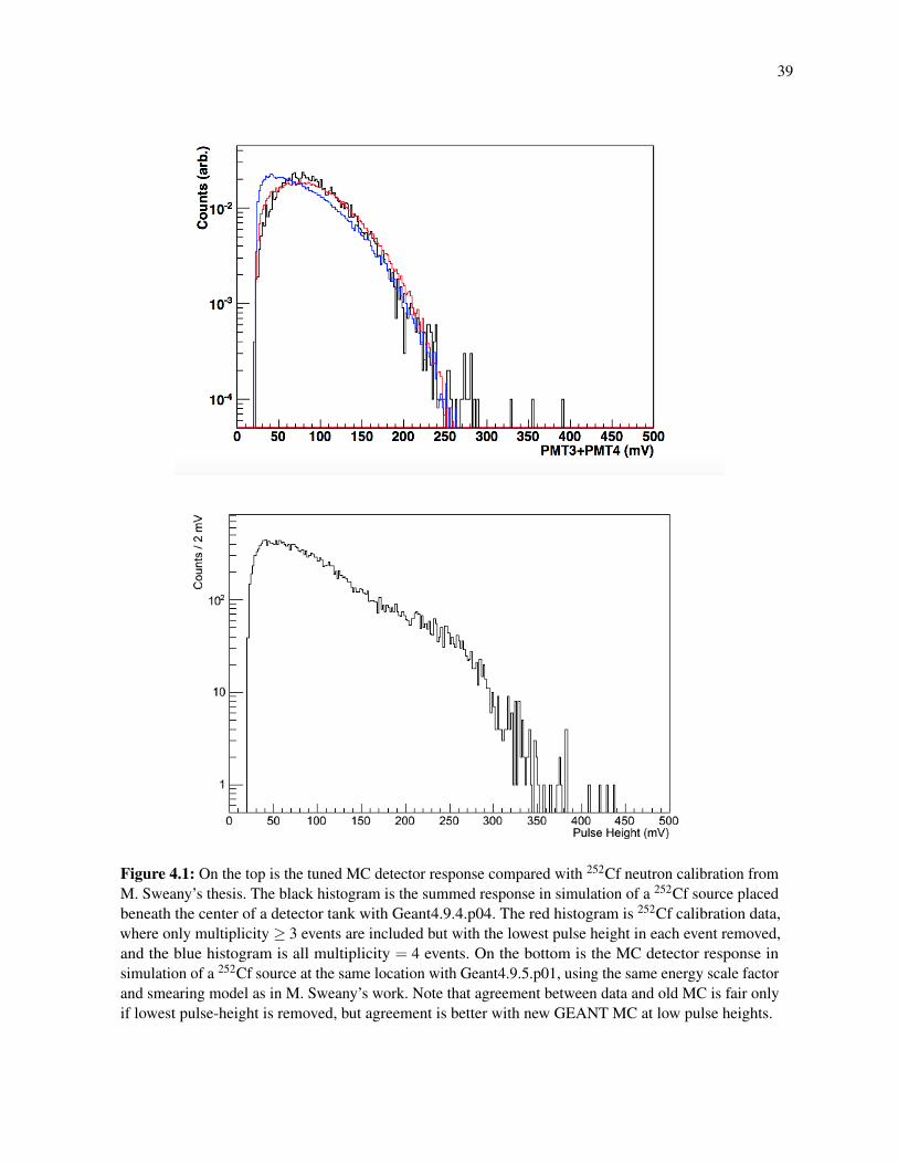
39

Figure 4.1: On the top is the tuned MC detector response compared with 252Cf neutron calibration fromM. Sweany’s thesis. The black histogram is the summed response in simulation of a 252Cf source placedbeneath the center of a detector tank with Geant4.9.4.p04. The red histogram is 252Cf calibration data,where only multiplicity ≥ 3 events are included but with the lowest pulse height in each event removed,and the blue histogram is all multiplicity = 4 events. On the bottom is the MC detector response insimulation of a 252Cf source at the same location with Geant4.9.5.p01, using the same energy scale factorand smearing model as in M. Sweany’s work. Note that agreement between data and old MC is fair onlyif lowest pulse-height is removed, but agreement is better with new GEANT MC at low pulse heights.

40

When M. Sweany tuned the energy scale and the convolution parameter, the MC software was

built with Geant4.9.4.p04, which calculates the Gd neutron-capture gamma energies using the

photon evaporation model [63]. As Geant4 updated to 9.5, the model associated with Gd neutron-

capture gamma emission was changed to determine the capture gamma final state via the Geant4

Neutron Data Library (G4NDL) [64][65][45]. With the updated Geant4 neutron-capture gamma

model but the same tuned parameters for pulse forming energy scaling and smearing, the simulation

of 252Cf neutron calibration results in a neutron capture pulse height spectrum shown in the bottom

of Figure 4.1. The shape of this spectrum actually better resembles the low energy peak in the

all-pulse included pulse height spectrum. The extra bump at relatively high energies implies that

high-energy gammas may be simulated by the updated Geant4. If the bump does not appear on the

252Cf neutron data, then the MC should need more smearing to obtain a smooth spectrum.

The updated model predicts a different individual gamma emission spectrum than that predicted

by the photon evaporation model. The individual gamma emission spectrum better resembles the

measured Gd neutron-capture gamma spectrum from literature [66], especially the high-energy

gamma lines. Figure 4.2 shows the comparison of individual gamma energy spectra predicted by

the two models, along with the measured gamma energy spectra of 155Gd, 157Gd [66], and natural

Gd [67]. This explains the extra bump around relatively high energies in the simulated neutron

spectrum with updated Geant4. More careful estimate of gamma background in the time of an

event according to measured gamma rate shows that the probability of coincidence with a gamma

pulse in a trigger neutron event is ∼ 0.07±0.003, far less than the level of ∼ 1 gamma per event.

Thus the assumption that the lowest pulse height of each event is due to gamma contamination is

not correct. The problem was with the old simulation; the pulse height spectrum predicted by the

updated Geant4 is much more similar to the all-pulse included spectrum at low energies.

The energy scale and smearing parameter tuned with inaccurate capture gamma model therefore

does not reflect correct properties of the detector. In addition, the PMTs have been rebalanced

and tuned to a slightly higher gain since May, 2011. The data taken before and after the change

41

Figure 4.2: The comparison of individual gamma emission spectra of gadolinium neutron capturesfrom Geant4 simulations and measurements. The simulated individual gamma emission spectrum fromGeant4.9.4.p04 (photon evaporation model) is shown in red, and the individual gamma spectrum fromGeant4.9.5.p01 (G4NDL) is shown in blue. The measured individual gamma spectrum from 155Gdand 157Gd together [66] is shown in black solid line, and the spectrum measured from natural Gd [67]is shown in black dashed line. G4NDL agrees with the measured spectra much better than photonevaporation model at high energy. At low energies, both models show discrepancy with the measuredspectrum. But gammas at such low energies are likely below Cherenkov threshold and therefore lessimportant.

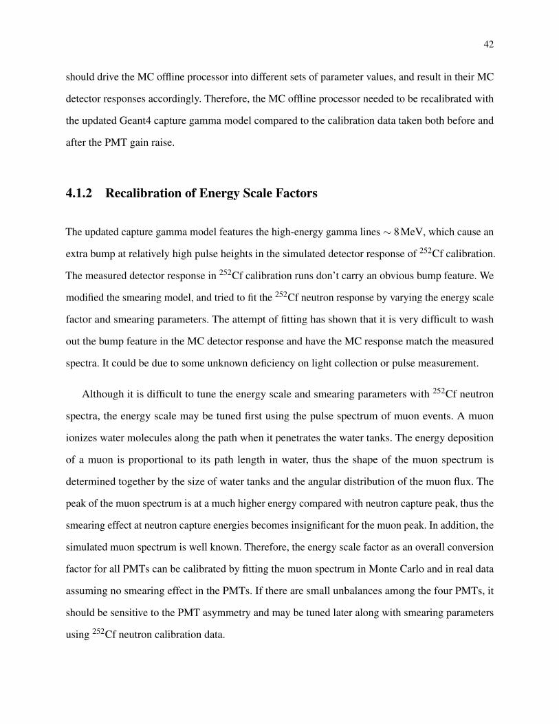
42

should drive the MC offline processor into different sets of parameter values, and result in their MC

detector responses accordingly. Therefore, the MC offline processor needed to be recalibrated with

the updated Geant4 capture gamma model compared to the calibration data taken both before and

after the PMT gain raise.

4.1.2 Recalibration of Energy Scale Factors

The updated capture gamma model features the high-energy gamma lines ∼ 8MeV, which cause an

extra bump at relatively high pulse heights in the simulated detector response of 252Cf calibration.

The measured detector response in 252Cf calibration runs don’t carry an obvious bump feature. We

modified the smearing model, and tried to fit the 252Cf neutron response by varying the energy scale

factor and smearing parameters. The attempt of fitting has shown that it is very difficult to wash

out the bump feature in the MC detector response and have the MC response match the measured

spectra. It could be due to some unknown deficiency on light collection or pulse measurement.

Although it is difficult to tune the energy scale and smearing parameters with 252Cf neutron

spectra, the energy scale may be tuned first using the pulse spectrum of muon events. A muon

ionizes water molecules along the path when it penetrates the water tanks. The energy deposition

of a muon is proportional to its path length in water, thus the shape of the muon spectrum is

determined together by the size of water tanks and the angular distribution of the muon flux. The

peak of the muon spectrum is at a much higher energy compared with neutron capture peak, thus the

smearing effect at neutron capture energies becomes insignificant for the muon peak. In addition, the

simulated muon spectrum is well known. Therefore, the energy scale factor as an overall conversion

factor for all PMTs can be calibrated by fitting the muon spectrum in Monte Carlo and in real data

assuming no smearing effect in the PMTs. If there are small unbalances among the four PMTs, it

should be sensitive to the PMT asymmetry and may be tuned later along with smearing parameters

using 252Cf neutron calibration data.

43

We do not have dedicated data runs tuned for recording muon events, but we may extract muon

events from the fast neutron search data. When a muon penetrates the water tanks and the lead stack,

there is a high chance for the muon to cause neutron spallations in the lead stack. The spallation

neutrons will then create a multiple neutron capture signature along with the initial high energy

pulse indicating the primary muon. These events are picked up by the event trigger on multiplicity.

To simulate the same type of events, we sampled the primary muons from the data set generated

by A. Reisetter using the MUSIC/MUSUN simulation package [68], based upon the geology and

geometry of the rock overburden and observations of the muon energy, momentum, and angular

distribution in the underground laboratory. In our simulation, the primary muons are initiated on top

of a 4 m rock layer above the cavern ceiling, and a subset of them will hit the NMM detector then

reproduce the reactions in the lead stack, thermalization and capture of neutrons, etc.

The energy of muon pulse is proportional to the muon’s path length in the water tanks. And a

muon with a longer path length in water generally has a longer path length in the lead stack, which

results in a greater chance to cause spallations and produce more secondary neutrons. Therefore, the

energy distribution of the selected muon events is not independent of the multiplicity of the events.

To make a fair comparison, we should compare the muon events in MC and real data with the same

multiplicity, or select the events with the same lower limit of multiplicity.

However, the multiplicity of the muon events in real data are skewed by afterpulsing. A large

pulse such as a muon induced pulse tends to cause several fake pulses, and raises the multiplicity

of the events. Many muons which did not create spallation neutrons would be still picked up by

the multiplicity-5 trigger due to afterpulsing. C. Nedlik’s study [69] has shown that afterpulses are

clusttered towards the initial muon pulse and there is almost no afterpulsing 50 µs after the initial

pulse. Here we use a time window of 50−100 µs since the initial large (> 1 V) pulse for event

selection. Events of MC and real neutron search data with two or more pulses in this time window

are selected, and the pulse height spectra are made of their initial large pulses. If the first pulse of an

event is not large enough (> 1 V), then ignore it but check the next pulses until find a large pulse.

44

Figure 4.3: Fit of muon pulse height spectrum in MC with the measured muon pulse height spectrumfrom low-gain data set for tuning the low-gain energy scale factor in MC offline processor. On the topis a comparison of muon pulse spectrum from the 1st neutron search run (black with error bars) andthe simulated muon spectrum with an energy scale factor of 2.2 mV/PE close to best fit (red histogram).The χ2 for the fit is calculated in the range of 1 V–7.4 V. The range is chosen so to select muon pulses,instead of neutron capture pulses, and also to exclude the PMT gain saturation near 8 V. On the bottomis the χ2s of the fits for several trial values of energy scale (blue squares), and a quadratic function to fitwith the distributions of the χ2s (magenta dashed line). The best-fit value of energy scale for the lowPMT gain, marked with a red vertical line, is found to be 2.26 mV/PE at the minimum of the quadraticfunction. The p-value of the best fit is 0.21.

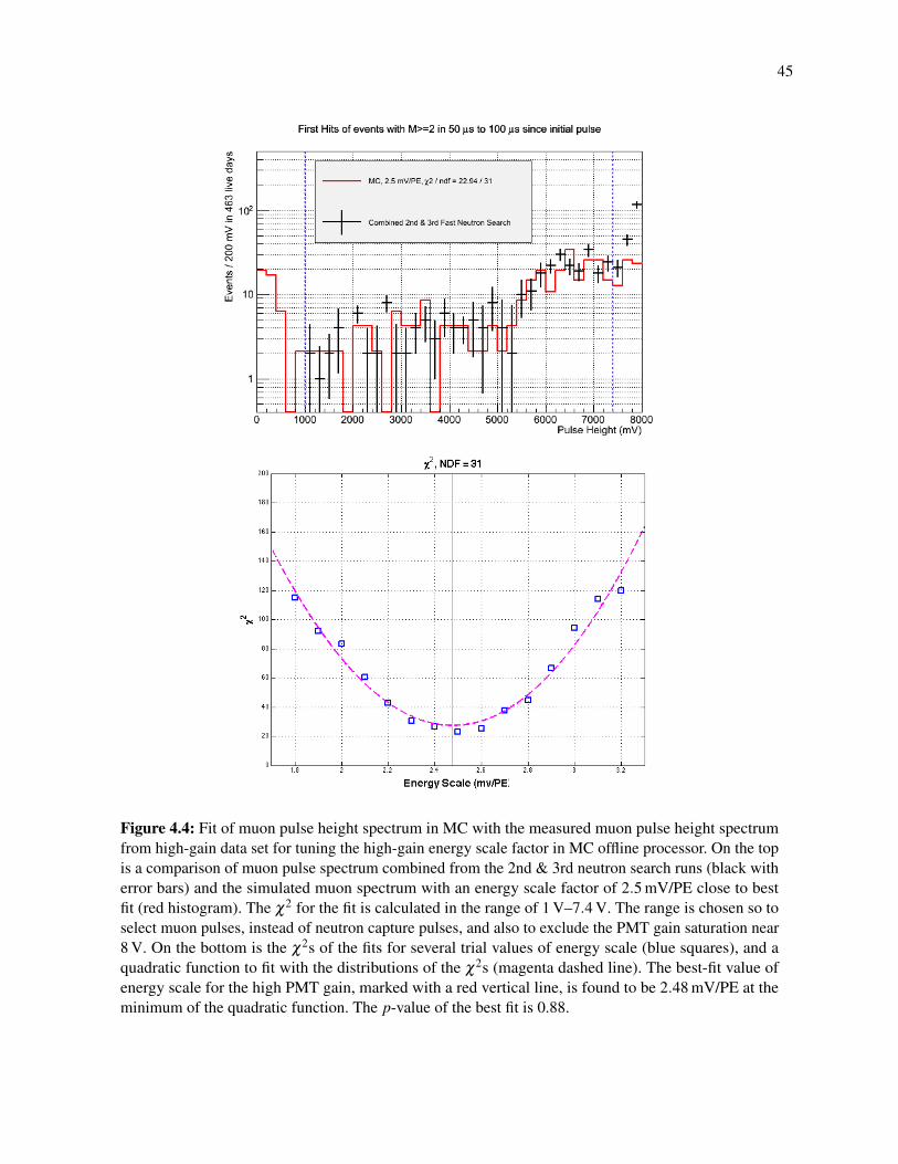
45

Figure 4.4: Fit of muon pulse height spectrum in MC with the measured muon pulse height spectrumfrom high-gain data set for tuning the high-gain energy scale factor in MC offline processor. On the topis a comparison of muon pulse spectrum combined from the 2nd & 3rd neutron search runs (black witherror bars) and the simulated muon spectrum with an energy scale factor of 2.5 mV/PE close to bestfit (red histogram). The χ2 for the fit is calculated in the range of 1 V–7.4 V. The range is chosen so toselect muon pulses, instead of neutron capture pulses, and also to exclude the PMT gain saturation near8 V. On the bottom is the χ2s of the fits for several trial values of energy scale (blue squares), and aquadratic function to fit with the distributions of the χ2s (magenta dashed line). The best-fit value ofenergy scale for the high PMT gain, marked with a red vertical line, is found to be 2.48 mV/PE at theminimum of the quadratic function. The p-value of the best fit is 0.88.

46

We do this to avoid missing the muon pulse of the events in which an accidental background gamma

is recorded before the muon pulse. We also apply a pulse height likelihood cut (will be discussed

in Chapter 5) to real data that the neutron likelihood parameter L > 0.99 to reject afterpulsing and

background gammas. With this method, we can make a fair comparison of muon spectra of MC and

real neutron search data.

We fit the pulse spectrum in MC with that in data by running the MC offline processor with

different energy scale factors and calculate the χ2s for the data-MC comparisons. Then the χ2 as a

function of the energy scale is fit with a quadratic function to determine the best fit energy scale

factor with the minimum of χ2. The results are shown in Figure 4.3 for the low-gain energy scale

and Figure 4.4 for the high-gain energy scale. On the top of both figures are the comparisons of

muon pulse spectrum in neutron search data and simulated muon spectrum with the energy scale

close to the best fit. On the bottom of both are the χ2s for several trial values of energy scale, and

quadratic functions to fit with the distributions of the χ2s. The low-gain fit, limited by the amount of

the data, is not very constraining. The values of energy scales at the minima of quadratic functions

are taken as the best fits, which is 2.26 mV/PE for low PMT gain, and 2.48 mV/PE for high PMT

gain.

4.1.3 Recalibration of Smearing Parameters

Once the overall energy scale has been tuned to provide the best fit with the muon pulse spectrum,

we apply it to process 252Cf simulation data. The comparison of MC and 252Cf calibration data can

provide information on the smearing parameters.

The 252Cf calibrations were performed by putting the 252Cf source under the top lead plate

beneath the center of the water tank for the calibration of the response in that tank and setting the

trigger on multiplicity of 3 in 60 µs. Calibrations for both the south tank and the north tank were

taken during the 1st fast neutron search (with relatively low PMT gains). After the PMT gains were

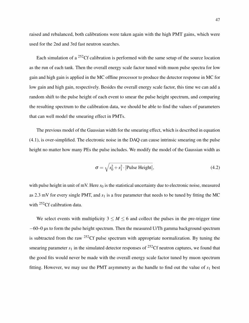
47

raised and rebalanced, both calibrations were taken again with the high PMT gains, which were

used for the 2nd and 3rd fast neutron searches.

Each simulation of a 252Cf calibration is performed with the same setup of the source location

as the run of each tank. Then the overall energy scale factor tuned with muon pulse spectra for low

gain and high gain is applied in the MC offline processor to produce the detector response in MC for

low gain and high gain, respectively. Besides the overall energy scale factor, this time we can add a

random shift to the pulse height of each event to smear the pulse height spectrum, and comparing

the resulting spectrum to the calibration data, we should be able to find the values of parameters

that can well model the smearing effect in PMTs.

The previous model of the Gaussian width for the smearing effect, which is described in equation

(4.1), is over-simplified. The electronic noise in the DAQ can cause intrinsic smearing on the pulse

height no matter how many PEs the pulse includes. We modify the model of the Gaussian width as

σ =√

s20 + s2

1 · [Pulse Height], (4.2)

with pulse height in unit of mV. Here s0 is the statistical uncertainty due to electronic noise, measured

as 2.3 mV for every single PMT, and s1 is a free parameter that needs to be tuned by fitting the MC

with 252Cf calibration data.

We select events with multiplicity 3 ≤ M ≤ 6 and collect the pulses in the pre-trigger time

−60–0 µs to form the pulse height spectrum. Then the measured U/Th gamma background spectrum

is subtracted from the raw 252Cf pulse spectrum with appropriate normalization. By tuning the

smearing parameter s1 in the simulated detector responses of 252Cf neutron captures, we found that

the good fits would never be made with the overall energy scale factor tuned by muon spectrum

fitting. However, we may use the PMT asymmetry as the handle to find out the value of s1 best

48

describing the smearing effect in PMTs. The PMT asymmetry is defined as

Asymmetry =[East PMT Pulse]− [West PMT Pulse][East PMT Pulse]+ [West PMT Pulse]

, (4.3)

for a pair of coincident pulses from the two PMTs of a water tank. The larger the value of s1 in the

offline MC processor, the wider the distribution of PMT asymmetries.

Small unbalances between east and west PMTs are known the exist. By fitting the channel

asymmetry, the energy scale factor should also be tuned slightly around the fit value with muon

spectrum comparison. I do this by adding and subtracting the same value on the energy scale factors

of east and west PMTs, called East-West Adjustment, respectively, and vary this small adjustment

to find the best fit with the asymmetry distribution, shown in Figure. 4.5, 4.6, 4.7, and 4.8. Table 4.1

summarizes the resulting best-fit East-West Adjustment values.

Once the best fit of the East-West Adjustment is found, we use it as a tuned parameter and vary

the smearing parameter s1. It is reasonable to assume all the PMTs have the same smearing for a

certain gain setting. We sum the χ2s for south tank and north tank at the same value of s1, and do

a combined quadratic least-square fit to find the best fit value of s1 for a certain gain setting. An

example of PMT asymmetry comparison between MC and 252Cf neutron data for the south tank

with low PMT gain is shown on the top of Figure 4.9, and the plot on the bottom of the same figure

shows the distribution of χ2 against the value of s1 for the PMT asymmetry comparisons with both

tanks combined. The best-fit value of s1 is chosen at the minimum of quadratic fit of the χ2s. The

same plots for high PMT gain calibration is shown in Figure 4.10.

The best fit values of the parameters of MC energy scale and smearing are summarized in

Table 4.1, including the adjusted energy scale factors of each single PMT, calculated by adding and

subtracting the East-West Adjustment on the overall energy scale factors.

The best fit of energy scales with proper adjustment between east and west PMTs and tuned

smearing parameters still result in the simulated 252Cf neutron spectra with the feature of a bump

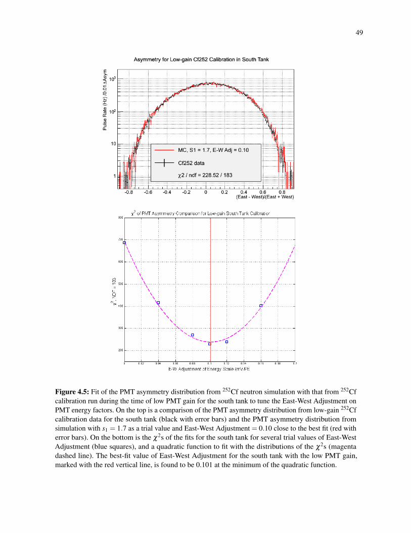
49

Figure 4.5: Fit of the PMT asymmetry distribution from 252Cf neutron simulation with that from 252Cfcalibration run during the time of low PMT gain for the south tank to tune the East-West Adjustment onPMT energy factors. On the top is a comparison of the PMT asymmetry distribution from low-gain 252Cfcalibration data for the south tank (black with error bars) and the PMT asymmetry distribution fromsimulation with s1 = 1.7 as a trial value and East-West Adjustment = 0.10 close to the best fit (red witherror bars). On the bottom is the χ2s of the fits for the south tank for several trial values of East-WestAdjustment (blue squares), and a quadratic function to fit with the distributions of the χ2s (magentadashed line). The best-fit value of East-West Adjustment for the south tank with the low PMT gain,marked with the red vertical line, is found to be 0.101 at the minimum of the quadratic function.

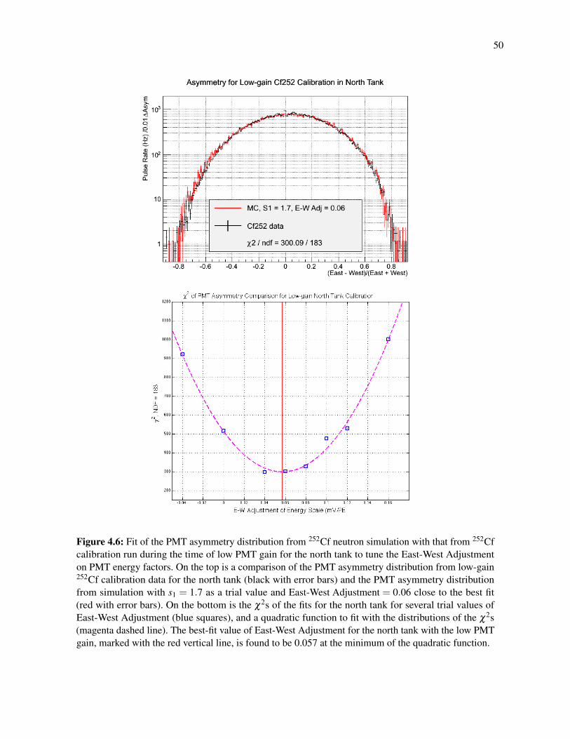
50

Figure 4.6: Fit of the PMT asymmetry distribution from 252Cf neutron simulation with that from 252Cfcalibration run during the time of low PMT gain for the north tank to tune the East-West Adjustmenton PMT energy factors. On the top is a comparison of the PMT asymmetry distribution from low-gain252Cf calibration data for the north tank (black with error bars) and the PMT asymmetry distributionfrom simulation with s1 = 1.7 as a trial value and East-West Adjustment = 0.06 close to the best fit(red with error bars). On the bottom is the χ2s of the fits for the north tank for several trial values ofEast-West Adjustment (blue squares), and a quadratic function to fit with the distributions of the χ2s(magenta dashed line). The best-fit value of East-West Adjustment for the north tank with the low PMTgain, marked with the red vertical line, is found to be 0.057 at the minimum of the quadratic function.

51

Figure 4.7: Fit of the PMT asymmetry distribution from 252Cf neutron simulation with that from 252Cfcalibration run during the time of high PMT gain for the south tank to tune the East-West Adjustmenton PMT energy factors. On the top is a comparison of the PMT asymmetry distribution from high-gain252Cf calibration data for the south tank (black with error bars) and the PMT asymmetry distributionfrom simulation with s1 = 2.0 as a trial value and East-West Adjustment = 0.10 close to the best fit(red with error bars). On the bottom is the χ2s of the fits for the south tank for several trial values ofEast-West Adjustment (blue squares), and a quadratic function to fit with the distributions of the χ2s(magenta dashed line). The best-fit value of East-West Adjustment for the south tank with the high PMTgain, marked with the red vertical line, is found to be 0.105 at the minimum of the quadratic function.

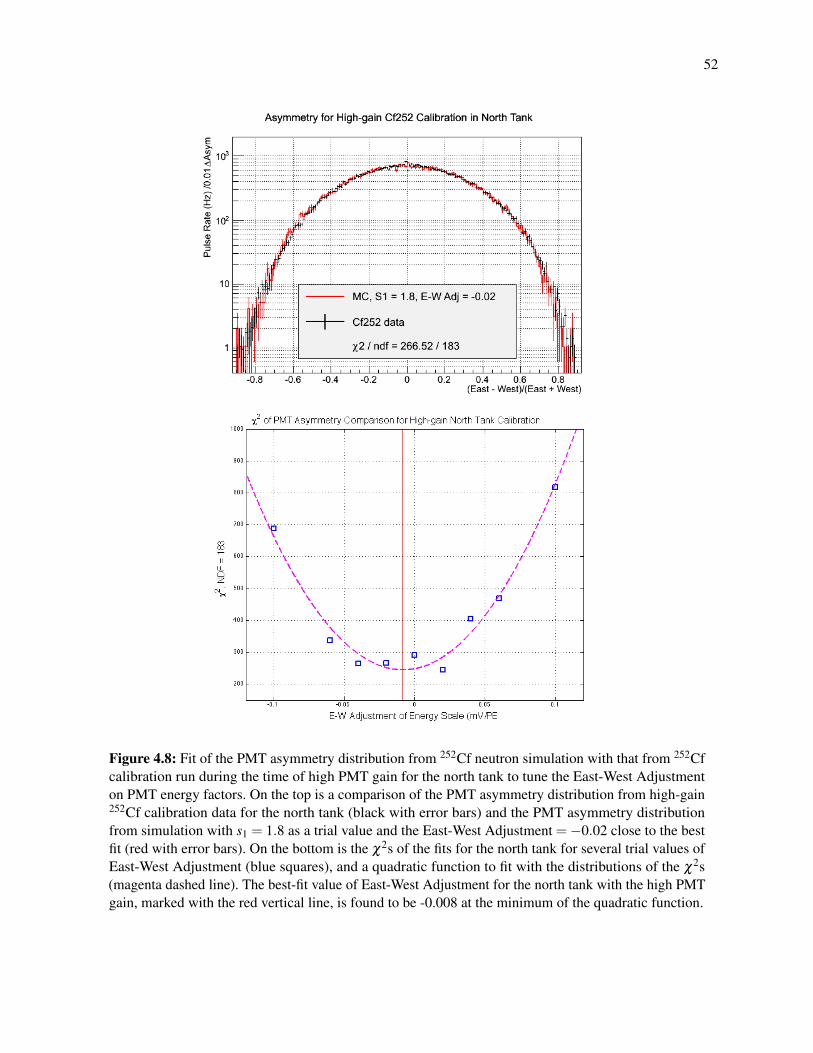
52

Figure 4.8: Fit of the PMT asymmetry distribution from 252Cf neutron simulation with that from 252Cfcalibration run during the time of high PMT gain for the north tank to tune the East-West Adjustmenton PMT energy factors. On the top is a comparison of the PMT asymmetry distribution from high-gain252Cf calibration data for the north tank (black with error bars) and the PMT asymmetry distributionfrom simulation with s1 = 1.8 as a trial value and the East-West Adjustment =−0.02 close to the bestfit (red with error bars). On the bottom is the χ2s of the fits for the north tank for several trial values ofEast-West Adjustment (blue squares), and a quadratic function to fit with the distributions of the χ2s(magenta dashed line). The best-fit value of East-West Adjustment for the north tank with the high PMTgain, marked with the red vertical line, is found to be -0.008 at the minimum of the quadratic function.

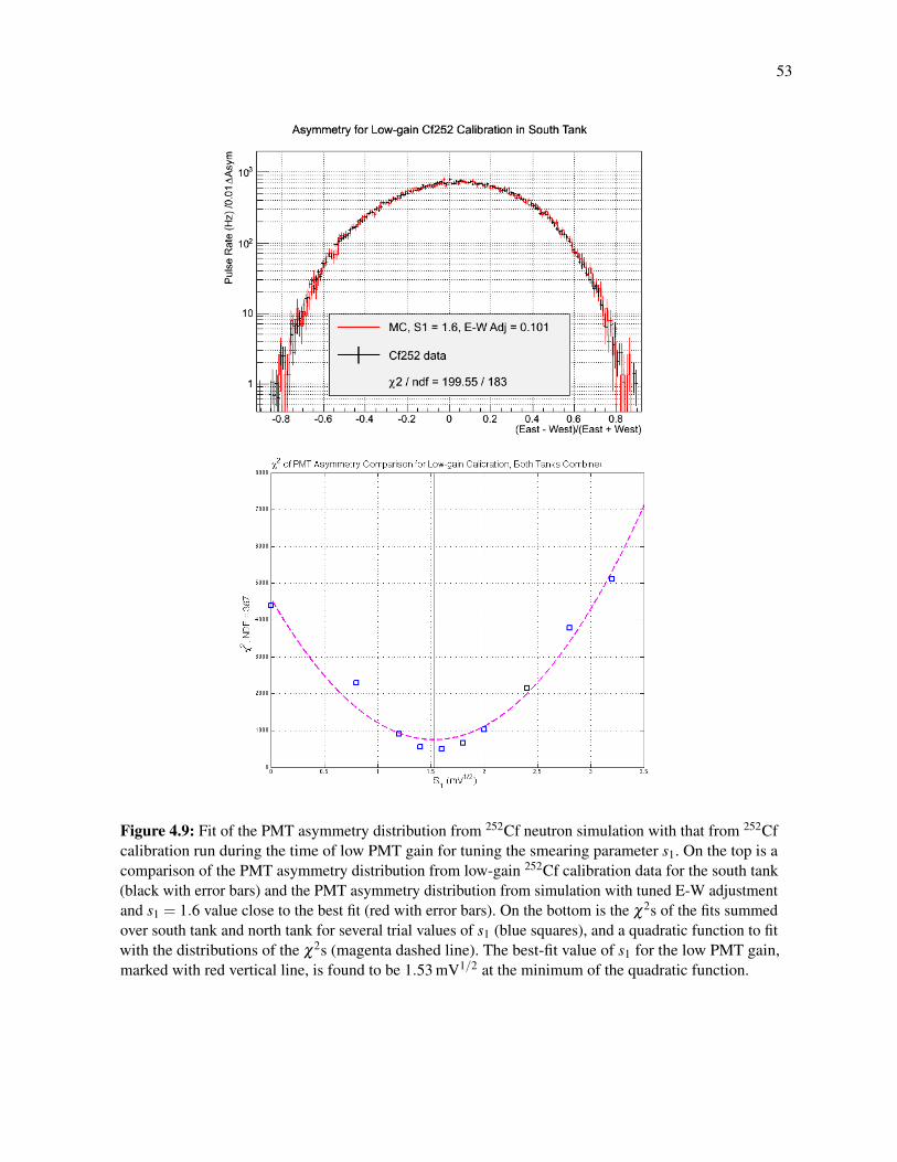
53

Figure 4.9: Fit of the PMT asymmetry distribution from 252Cf neutron simulation with that from 252Cfcalibration run during the time of low PMT gain for tuning the smearing parameter s1. On the top is acomparison of the PMT asymmetry distribution from low-gain 252Cf calibration data for the south tank(black with error bars) and the PMT asymmetry distribution from simulation with tuned E-W adjustmentand s1 = 1.6 value close to the best fit (red with error bars). On the bottom is the χ2s of the fits summedover south tank and north tank for several trial values of s1 (blue squares), and a quadratic function to fitwith the distributions of the χ2s (magenta dashed line). The best-fit value of s1 for the low PMT gain,marked with red vertical line, is found to be 1.53 mV1/2 at the minimum of the quadratic function.

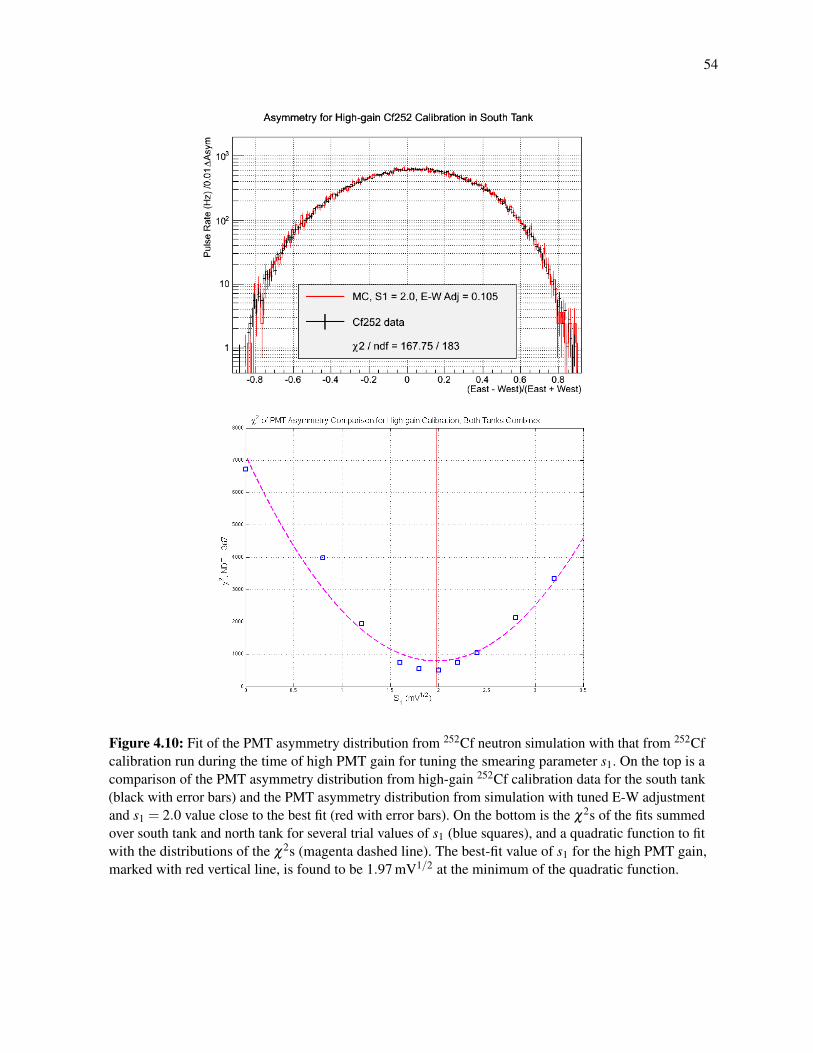
54

Figure 4.10: Fit of the PMT asymmetry distribution from 252Cf neutron simulation with that from 252Cfcalibration run during the time of high PMT gain for tuning the smearing parameter s1. On the top is acomparison of the PMT asymmetry distribution from high-gain 252Cf calibration data for the south tank(black with error bars) and the PMT asymmetry distribution from simulation with tuned E-W adjustmentand s1 = 2.0 value close to the best fit (red with error bars). On the bottom is the χ2s of the fits summedover south tank and north tank for several trial values of s1 (blue squares), and a quadratic function to fitwith the distributions of the χ2s (magenta dashed line). The best-fit value of s1 for the high PMT gain,marked with red vertical line, is found to be 1.97 mV1/2 at the minimum of the quadratic function.

55

Figure 4.11: The comparison of 252Cf neutron pulse height spectra from simulations with tuned PMTenergy scale and smearing parameters in this work (red) and the pulse height spectra measured in 252Cfneutron data (black). On the top is the comparison for low PMT gain using south tank data. On thebottom is the comparison for high PMT gain using south tank data.

56

Table 4.1: Summary of best-fit values of energy scales and smearing parameters in the MC offlineprocessor. The values of overall energy scale result from the fits shown in Figure 4.3 and 4.4. TheEast-West Adjustment is the value added to the east PMT and subtracted from the west PMT of the bestfit energy scale factor for a PMT gain setting, to fine-tune the energy scale factors for the single PMTs.The fits of East-West Adjustment are shown in Figure 4.5, 4.6, 4.7, and 4.8. Smearing paremeters s1 isdefined with Eq. (4.2) and the fits for the values are shown in Figure 4.9 and 4.10.

OverallEnergyScale(mV/PE)

East-WestAdjustment(mV/PE)

Single PMT Energy Scale(mV/PE) Smearing

Parameters1 (mV1/2)South North SE SW NE NW

Low-gain 2.26 0.101 0.057 2.361 2.159 2.317 2.203 1.53High-gain 2.48 0.105 -0.008 2.585 2.375 2.472 2.488 1.97

around ∼ 250mV, as shown in Figure 4.11 for south tank data of both low and high PMT gains.

This is definitely not a perfect reproduction of the detector response. The reason for this remaining

discrepancy is likely from the optical part of simulation. An all-included muon simulation resulting

in a large amount of data was performed with the updated version of Geant4 but the optical

parameters had been tuned with older version of Geant4. Thus to study the results of the all-included

muon simulation, we could only tune the parameters in the offline processor. However, the spectra

show good agreement at pulse heights less than∼ 60mV, at which the trigger rate in MC is sensitive

to the energy scale and smearing. The MC parameters tuned in this work would be able to minimize

the systematic errors of the event rate in the simulation. The pulse height distributions of neutron

captures are used to construct a pulse height likelihood function and a neutron-selection cut. But the

function and cut are built with the measured spectra and applied to real neutron search data. On the

other hand, the background leakage of the cut should be estimated with simulated muon events and

sampled with U/Th gamma PDF. Therefore the disagreement at higher pulse heights will not be

crucial to the neutron search data analysis.

57

4.2 A Comprehensive Simulation of Cosmic Muons and Muon-induced

Neutrons

In order to understand the muon background, as well as the production and detection of the high-

energy neutrons, instead of simulating the detector response of muon background and parametrized

high-energy neutrons separately, we have performed a comprehensive muon simulation. The idea is

to propagate cosmic-ray muons on top of a rock layer and directly simulate the interaction of muons

in the cavern rock. The simulation includes the process of muon-induced hadronic showers and the

initiation of the high-energy neutrons, which is the signal we are searching for in this experiment.

It naturally incorporates the correlation between the high-energy neutron and the initial muon,

i.e., help study the rate of a clean neutron-capture signal and the rate of a neutron-capture event

accompanied by a direct hit of the initial muon on the detector.

The study of this simulation will serve two purposes. It can help the analysis of the fast neutron

search data. It may reveal informative MC truth, which is useful for improving the data selection

cuts, and the understanding of the content of detected events. Another purpose is to provide a

simulated multiplicity spectrum, and use it to benchmark the measured multiplicity distribution.

This comparison is one of the fundamental goals of the Neutron Multiplicity Meter experiment.

4.2.1 Simulation Setup

In the MC software, the detector model is placed in the cavern at the location of the NMM in the

Soudan cavern. The cavern is 32 m× 14.5 m large and 11 m high. The cavern model is surrounded

by rock with 4 m thickness on its six sides, making a 40 m× 22.5 m large and 19 m high “world” in

the Geant4 MC software. In the comprehensive simulation, muons are initiated on the top surface

and four sides of the “world”. Before propagating into the cavern, the muon may cause a hadronic

shower and/or spallations in the 4 m thick ceiling and side wall rock, and the high-energy neutrons

58

generated by these processes in the rock surrounding the cavern are naturally included in the MC.

The initial energy and incident angle of each muon is sampled from results of a simulation with

cosmic-ray muons propagating from ground surface to the depth of the Soudan mine (2090 m.w.e.)

using the MUSIC/MUSUN package [68]. The energy spectrum and angular distribution of the

primary muons are shown in Figure 4.12. The energy spectrum and the angular distribution shown

here are correlated, as muons at greater angles (smaller cosθ ) are less likely to reach the depth, but

those that do reach the depth are more likely to carry higher energies.

There are 3.384×107 primary muons simulated in this work, which covers the top surface as

well as the four sides of the MC world. Of these, there are 2.159×107 primary muons started on

the top surface. A flux through a horizontal surface should be used to compare with the measured

muon flux at the Soudan site, (2.0±0.2)×10−7 cm−2 s−1 [53]. Therefore, the live time of the

comprehensive muon simulation is estimated as

2.159×107

2.0×10−7 cm−2 s−1× (40m×22.5m)= 1.20×107 s≈ 138.8days. (4.4)

Here the horizontal dimension of the MC world is used.

The MC software records not only the optical photons that hit the surface of PMTs as the raw

data of detector response, but also the relevant MC truth, including position and momentum of

any particle that is traversing the surfaces of water tank, lead stack, or cavern wall, as well as the

positions and times of neutron captures.

4.2.2 Data Processing

The simulation records the times when optical photons hit the PMT surfaces relative to the beginning

of each event. The first step of data processing is to find pulses from the raw simulated data of

optical photon timing. The recorded photons are randomly selected with a probability based on the

quantum efficiency of the PMT as a function of the photon wavelengths. The selected photons are

59

Figure 4.12: Primary muons in the comprehensive simulation. On the top is the energy spectrum of theprimary muons used in this simulation. On the bottom is the angular distribution of the primary muonsshown in cosine of the zenith angle, cosθ . The initial states of the muons are sampled from the results ofa MUSIC/MUSUN simulation with cosmic-ray muons propagating from ground surface to the depth ofthe Soudan mine.

60

further recorded as photoelectrons. The processor then goes over the sequence of the photoelectron

times in each PMT. When it finds a photoelectron, it groups all the later photoelectrons within

250 ns of the leading photoelectron as a pulse and counts as number of PEs in the pulse. Then it

repeats the same way of combining PEs into pulses for the rest of the event. This forms a trace of

pulses counted in PEs. The time of a pulse is calculated as the average time of all the photoelectrons

within the pulse.

The pulses in real data are measured in volts. To be able to compare with data, the PE counts of

simulated pulses need to be converted to mV by multiplying by an energy scale factor and applying

a Gaussian random offset with a width controlled by smearing parameters. The energy scale factors

and smearing parameters have been discussed in Section 4.1, and the tuned parameters shown in

Table 4.1 are used to process the comprehensive muon simulation data.

For any single PMT channel, there is a 10 mV threshold for the pulse trigger in the detector DAQ

settings. In the MC, pulses are therefore required to be at least 10 mV to “trigger”–to be further

recorded. According to the parameters in Table 4.1, this is equivalent to triggering on ∼ 5PEs.

The triggered single PMT pulses are matched with the pulse trace in the other PMT of the

same water tank to find coincidences in timing. If two pulses from both PMTs are within 250 ns of

each other, we say that they are coincident pulses. The average pulse time of the two coincident

pulses is called the coincident pulse time. All the coincident pulse times for the two PTMs form the

coincident pulse trace of the water tank. The pulse of and individual PMT not coincident with any

pulse in the other PMT will not be recorded in the coincident pulse trace. The pulse height sums

over the coincident pulse pairs form a trace of summed pulse heights for the water tank.

The processor merges the coincident pulse traces of the two tanks into one pulse trace in

chronological order for both coincident pulse times and summed pulse heights. There is a special

circumstance that two coincident pulses in one tank are also coincident in time with the two

coincident pulses in the other tank. We call it a quadruple coincidence. A set of quadruple coincident

61

pulses are usually caused by the same particle interaction. For quadruple coincident pulses, the

pulse heights are added up again to form a single summed pulse height, and the pulse times are

taken as the average over the two tanks.

With the procedure described above, the raw data of PMT photon hits are reduced to vectors

(or traces) of coincident pulse timings and summed pulse heights. They are stored, along with the

individual PMT pulse traces of timing and pulse heights from all four PMTs, to form the data

structure of the event.

4.2.3 Monte Carlo Truth Analysis

It is important to link the pulse with its source recorded in Monte Carlo truth–the interaction in the

detector that caused the pulse. For instance, a neutron capture in a water tank would illuminate the

tank with Cherenkov light induced by capture gamma emission and fire the PMTs. Charged particles

may ionize water or emit Cherenkov light when they pass through the water tanks, but instead

of directly recording the interactions, particles are recorded when they traverse the boundaries of

the water tanks, bottom lead, and cavern. All the available MC truth can be used to determine the

sources of pulses.

P U L S E - T A G G I N G A L G O R I T H M

The algorithm of tagging the pulse with its source is based on matching their timing. Figure 4.13

shows the distribution of time difference from a pulse back to the closest MC truth “event”, i.e.

either a neutron capture in water tanks or a charged particle crossing the boundary of water tanks.

The distribution of the time differences shows that the source events cause the resulting pulses in

∼300 ns. Thus 300 ns is a proper time window for finding the coincidence between a pulse and its

source. Any interaction recorded in MC truth taking place earlier than the 300 ns time window may

be considered uncorrelated with the pulse.

62

Figure 4.13: The difference in time between a pulse and the MC truth “event” taking place right beforethe pulse time. The MC truth “event” can be a neutron capture (in black), or any charged particle crossingthe boundary of water tanks (in colors). In the plot, the timing difference is taken relative to the timeof the pulse. The peaks in the time difference distributions show the correlation between an MC truth“event” and the pulse. The timing difference at the major peak is related to the size of the water tanks.The neutron captures take place with in ∼ 300ns prior to the pulse. The flat tails for all types of MCtruth “event” show the cases that the pulses are unrelated to the MC truth. The reason of the multiplepeaks for charged particles is unclear.

63

The procedure is as follows.

1. First check in the 300 ns time window prior to the pulse to see if there is any neutron capture

in the water tanks. If a neutron capture in the water tanks is found, the pulse is tagged as a

neutron capture pulse.

2. If no neutron capture is found, then check if there is any charged particle traversing the

boundary and flying into the water tanks. Label the pulse as “muon pulse” if the charged

particles found in the 300 ns pre-time window include a muon. Tag the pulse as a “secondary

charged particle pulse” if one or more charged particles, but no muons, are found. A muon

pulse should be considered differently from the secondary charged particles induced by the

muon.

3. If neither a neutron capture, nor any incident charge particle is found, which happens in rare

cases, then consider the pulse as caused by a neutron capture in the acrylic wall of the water

tanks. That is because only neutron captures taking place in water were recorded when the

simulation was running, but the wall of the water tanks made of acrylic can also capture

neutrons with the hydrogen nuclei. In the simulation, the logical boundary of the water tanks

was set as the outer boundary of the acrylic tank wall. Given this fact, it is reasonable to tag a

pulse associated without any recorded source in 300 ns pre-time window in MC as a neutron

capture pulse with the capture happened in acrylic tank wall.

T Y P E S O F E V E N T S

Given the pulses tagged with their sources as neutron capture, muon, or secondary charged particles,

the detector events can be divided into different types according to the composition of pulses.

1. Fast neutron events. When an event consists only of neutron capture pulses, it is a detection

of the secondary neutrons liberated by the incident fast neutron into the lead target. It is so

identified as a fast neutron event, which is what we ideally search for in the NMM experiment.

64

2. Muon events. If an event consists only of muon pulses, or of any muon pulse plus secondary

background pulses, it is considered as a muon event.

3. Secondary charged particle events. If an event consists only of secondary charged particle

pulses, it is called a secondary charged particle event. When the muon travels in cavern rock,

it creates many secondary particles. These particles may have chance to scatter and travel into

the water tanks, even when the muon itself misses.

4. Muons accompanied with neutron captures. A muon that left a pulse means it penetrates

one or both water tank(s). In the meantime, the muon is very likely to hit the lead stack as

well. If an event is found as a muon pulse with multiple neutron capture pulses, the secondary

neutrons are very likely released directly by the muon striking the lead target. These neutron

captures are not a detection of a fast neutron, and this type of event is not considered as signal.

If it happens that the muon passes one of the water tanks by a small corner with a path length

short enough, to fire a pulse small enough to pass the muon rejection cut, then the subset of

this type may mimic the signal type of real fast neutrons. In this case, we call it a clipping

muon.

5. Skewed fast neutrons. If an event consists of mostly neutron capture pulses, but also one

or two secondary background pulses, in contrast to the last type, the lead target is almost

certainly not hit by the muon, thus the detection of multiple neutron captures is indeed the

signal of a fast neutron, but with one or two background pulses that skews the counting of the

multiplicity.

R E S U L T S

With the classification of events discussed above, the MC truth of each type of events can be studied

to help understand the real data taken in the NMM experiment.

In Figure 4.14 the multiplicity spectrum of each event type discussed above is shown in a

65

Figure 4.14: Pulse multiplicity spectra of the events in different types based on MC truth. All the typesof events in MC truth are shown in colors described in the legend. A dashed black vertical line shows thetrigger threshold on pulse multiplicity at 5. The scales in Y-axis of all spectra are based on their originalcounts in the MC.

66

color histogram for the comprehensive muon simulation results, processed with lower PMT gain

parameters. The detector trigger on multiplicity at threshold 5 is indicated with the dashed black line

in the figure. Two major types of backgrounds, muon events and secondary charged particle events,

which mostly fire one or two pulses, are completely suppressed by the threshold on multiplicity.

Note in the real data of the experiment, an initial pulse due to a muon or other charge particles may

be energetic enough to cause severe afterpulsing, so the multiplicity may exceed 5 and trigger an

event.

Spectra of the maximum pulse of each event are plotted for all five types of events in Figure 4.15.

On the top the maximum pulse spectra are shown up to 10 V. The muon peaks are clearly shown

in the muon events and muons accompanied with neutron captures (in green and red). The events

involved with secondary charged particle show a different shape of high energy peaks compared

with the muon peaks (in cyan and magenta). Some high energy pulses shown in the fast neutron

events, which are too large for Gd neutron capture emissions, are likely due to mis-tagging to the

pulses. For example, a large pulse induced by a muon or a high-energy charged particle happens

to be closer to a neutron capture in timing than the real source would be mis-tagged as a neutron

capture pulse. But the mis-tagged pulses are rare compared with correctly tagged capture pulses.

On the bottom the pulse spectra are shown up to 500 mV for a better look at low energies. The

maximum pulse spectrum of fast neutron events is consistent with the detector responses measured

and simulated in 252Cf calibration runs. The skewed fast neutrons are less populated in the low

energy pulse region than fast neutron events as the maximum pulses of the skewed fast neutrons are

mostly from high-energy charged particles, but the spectrum is relatively similar to neutron captures.

Muons accompanied with neutron captures have a small population at the low energy region. With

a muon rejection cut at 300 mV or even smaller volt, most of muons accompanied with neutrons

captures will be removed from the candidate set.

It is useful to check the distribution of pulse timing in the events. The pulse timings of neutron

capture pulses and muon pulses since the beginning of each event are plotted in Figure 4.16 for

67

Figure 4.15: Pulse spectra of the maximum pulse in each event for different event types (in colors asdescribed in legends). On the top is shown in the pulse height scale up to 10 V and binned per 100 mV.On the bottom is shown in the scale up to 500 mV and binned per mV. The scales on Y-axis of allspectra are based on their original counts in the MC. Note that gigh-energy muons are minimum ionizingparticles, therefore the peak of muon pulses at ∼5.4 V corresponds to the height of the water tanks,76.2 cm, which is the path length of most muons traversing the water tanks, and the correspondingenergy deposition is estimated to be ∼152 MeV, based on the minimum stopping power of muon inwater, 1.992 MeVcm2/g [70]. The peaks of charged particles are similar to those of muons, but theshape is slightly different. The large pulses in fast neutron events are likely due to mis-tagged muons orhigh-energy charged particles.

68

different types of events except for secondary charged particle events. Neutron capture pulses (in

solid lines) feature a rising time of ∼ 5µs, which originates from the time delay from the initiation

of interactions to the first capture of secondary neutrons, and an exponential fall time, which

describes the process of every moderated neutron in the water tank finding a gadolinium nucleus

and being captured. The neutron capture timing distributions in different event types are identical,

providing a sanity check that the tagging of neutron capture pulses is correct. Muon pulses (in

dashed lines) appear only in a very prompt time window, 0 – ∼0.5 µs. In fact, the cosmic muons are

very penetrating and never back-scatter into the detector. It is also confirmed in the MC that the

muon pulse takes only the first position of the event, and no interactions of any other particle with

the detector ever take place earlier than the muon in the event.

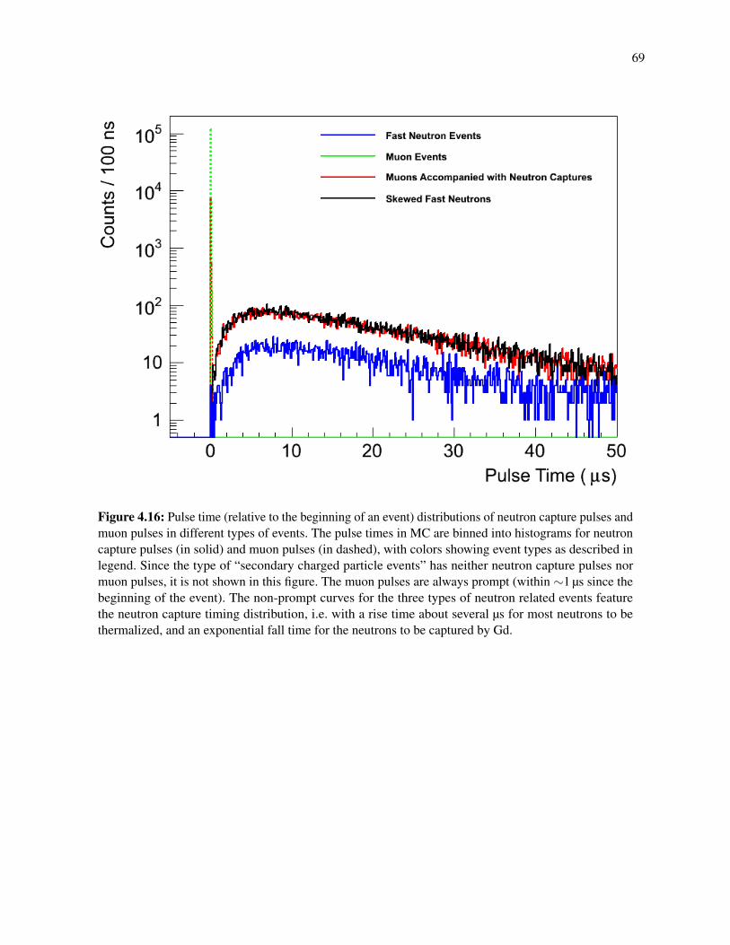
69

Figure 4.16: Pulse time (relative to the beginning of an event) distributions of neutron capture pulses andmuon pulses in different types of events. The pulse times in MC are binned into histograms for neutroncapture pulses (in solid) and muon pulses (in dashed), with colors showing event types as described inlegend. Since the type of “secondary charged particle events” has neither neutron capture pulses normuon pulses, it is not shown in this figure. The muon pulses are always prompt (within ∼1 µs since thebeginning of the event). The non-prompt curves for the three types of neutron related events featurethe neutron capture timing distribution, i.e. with a rise time about several µs for most neutrons to bethermalized, and an exponential fall time for the neutrons to be captured by Gd.

70

4.2.4 Muon Rejection Cut Study

The facts found in the comprehensive muon simulation may help improve the muon rejection cut.

The previous design of the muon rejection cut was to require that the maximum pulse height of

any pulse in the event be smaller than 300 mV. It is relatively inefficient to remove muon events

by cutting on all pulses in the event. The analysis of the comprehensive muon simulation confirms

that the detector response of the muon is prompt in time and always fires as the first pulse in any

muon-involved event in the MC. A smarter way to remove muon events is to set the cut only on the

first pulse of the event. This way of cutting can avoid removing neutron capture events in which

there is any non-prompt pulse greater than the cut threshold, and focus better on the muon pulse. In

the real data analysis, however, there is an non-negligible chance to record a pulse induced by a

background gamma ahead of the muon pulse, making the muon pulse the second pulse of the event.

The rate of n gammas to be coincident ahead of a muon can be estimated as

R(nγ +µ) =(rγ ·100µs)ne−rγ ·100µs

n!· rµ , (4.5)

which is the Poisson probability for n gamma pulses with the gamma pulse rate rγ occuring in

100 µs time inteval, multiplying by the muon pulse rate rµ . Muon events usually trigger at the 4th

coincident after-pulse after the primary muon pulse, but the trigger time is very close to the time

of the muon pulse, so it is reasonable to approximate pre-trigger time with 100 µs. The gamma

pulse rate for two tanks together is approximately 700 Hz for the low PMT gain and 850 Hz for

the high PMT gain; muon pulse rate is estimated using fast neutron search data to be 4.7 mHz for

the low-gain, and 8.0 mHz for the high-gain. Then the estimated 1γ + µ rate is 3×10−4 Hz for

the low-gain and 6×10−4 Hz for the high-gain; the estimated rate of 2γ +µ events is 1×10−5 Hz

for the low-gain and 3×10−5 Hz for the high-gain. Thus it is necessary to set the cut on the first

two pulses of the event. With this style of cutting, the cut threshold may be tightened to remove

muon events more efficiently without losing efficiency on neutron capture events. This change is

71

especially important for higher-multiplicity events.

To quantify the performance of both styles of muon cuts, the efficiency of the muon cut on

passing neutron capture events is calculated by Monte Carlo simulation. For a given value of

multiplicity M, M pulses are sampled according to the pulse height distribution measured in 252Cf

calibration data to form an event. The efficiency of each case is calculated by applying the cut

to 106 sampled events to count the pass fraction of neutron capture events. The efficiencies as a

function of cut position on pulse height are shown in Figure 4.17 and Figure 4.18 for low PMT

gain and high PMT gain, respectively. In each figure, the left column shows the efficiencies of

the muon cut on the maximum pulse of the event, and the right column shows the efficiencies

of the muon cut on the first two pulses of the event. The calculation (in red curve) is compared

with the measurement from 252Cf calibration data (in data points and error bars). The comparisons

are shown for multiplicity 3, 4, 5, and 6. Efficiencies for higher multiplicities are calculated but

not measured (and not shown here) since there is not large enough statistics from the events with

higher multiplicities in 252Cf calibration data. The measurements and calculations agree well on

high pulse heights (> 200mV), but show discrepancies at low pulse heights. The discrepancies are

presumably due to background gamma pulses. The expected background gamma distribution has

been subtracted from the pulse height distribution measured in calibration data. The background-

subtracted pulse height distribution is used in calculation and neutron likelihood construction. But

when the cut efficiencies are measured in 252Cf data, the cut applies to neutron capture events mixed

with background gamma events. Background gamma pulses have significantly lower pulse heights,

and therefore have a higher pass fraction. The mixture of the background gamma population in the

testing events makes the measured pass efficiencies higher than the calculations.

The cut efficiency on neutron capture events decreases as the cut is tightened, set to a lower

pulse height. The efficiencies of the cut on the maximum pulse drop faster than the cut on the first

two pulses as the cut position decreases, and drop more drastically as the multiplicity increases,

while the efficiency of the cut on the first two pulses is not sensitive to multiplicity. In the case of

72

Figure 4.17: Efficiencies of muon cut for neutron capture events with low PMT gain as a function ofthe cut pulse height, compared for both cut-on-maximum style (left column) and cut-on-first-two style(right column), shown for events of multiplicity 3, 4, 5, and 6 (in each row from top to bottom). Thecalculated efficiencies from MC sampling are shown in the red curves, while the efficiencies measuredwith Cf neutron data are shown in black (source under source tank) and blue (source under north tank)data points.

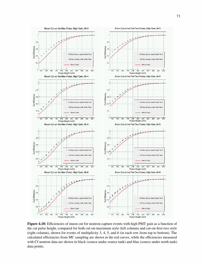
73

Figure 4.18: Efficiencies of muon cut for neutron capture events with high PMT gain as a function ofthe cut pulse height, compared for both cut-on-maximum style (left column) and cut-on-first-two style(right column), shown for events of multiplicity 3, 4, 5, and 6 (in each row from top to bottom). Thecalculated efficiencies from MC sampling are shown in the red curves, while the efficiencies measuredwith Cf neutron data are shown in black (source under source tank) and blue (source under north tank)data points.

74

low PMT gain, if the muon cut is tightened to 200 mV, the cut on the maximum pulse will have

the efficiency dropped to ∼ 90% for events of multiplicity 5, and even lower for events of higher

multiplicities, while the cut on the first two pulses will drop the efficiency only to ∼ 96.7%, and it is

not sensitive to multiplicity. Therefore, redesigning the cut style as applying on the first two pulses

and tightening to 200 mV is affordable in the sense of not losing much efficiency on neutron capture

events. In the case of high PMT gain, the cut position is tuned to 250 mV to get the same efficiency.

According to the calculation earlier in this section, the chance for the muon pulse to occur at the

third place, i.e. as a 2γ +µ event, is much smaller than at the second place, but it still results in,

say, ∼137 events in the 158 live days of the 1st fast neutron data. We add a cut at 300 mV on the

third pulse to remove this type of events. Neutron pulses are below 300 mV, so adding the cut on

the third pulse does not affect the estimation of the cut efficiency.

As discussed in subsection 4.2.3, the basic muon events do not survive the multiplicity trigger

requirement in the MC. In addition to removing the muon events that triggered in the real data

due to afterpulsing, the main role of the muon rejection cut is to remove the events of low pulse

height muons accompanied by neutron captures, known as clipping muons. The pulse spectrum of

simulated muon pulses is shown in Figure 4.19 for all muons accompanied with neutron captures

(in blue) and the same type of events but surviving multiplicity trigger requirement (in red). The

left column of plots show the spectra for low PMT gain, while the right column of plots show the

spectra for high PMT gain. The top plots, which show the spectra with scale up to 10 V, indicate

that the shapes of the spectra before and after the multiplicity trigger applied are nearly identical.

From the bottom plots, which focuses on the low pulse height end, it is shown that, in case of low

PMT gain, there are only 7 clipping muon events surviving both multiplicity trigger and a muon

rejection cut at 200 mV in the comprehensive muon simulation with 138.8 days of live time. In the

case of high PMT gain, 8 clipping muons survive the muon rejection cut at 250 mV. The muon

spectra of the events before applying the trigger requirement (the blue histograms) can be used to

estimate how much the clipping muon rate can be reduced by tightening the cut in the real data

analysis. Tightening the muon cut from 300 mV to 200 mV is expected to remove ∼ 25% of the

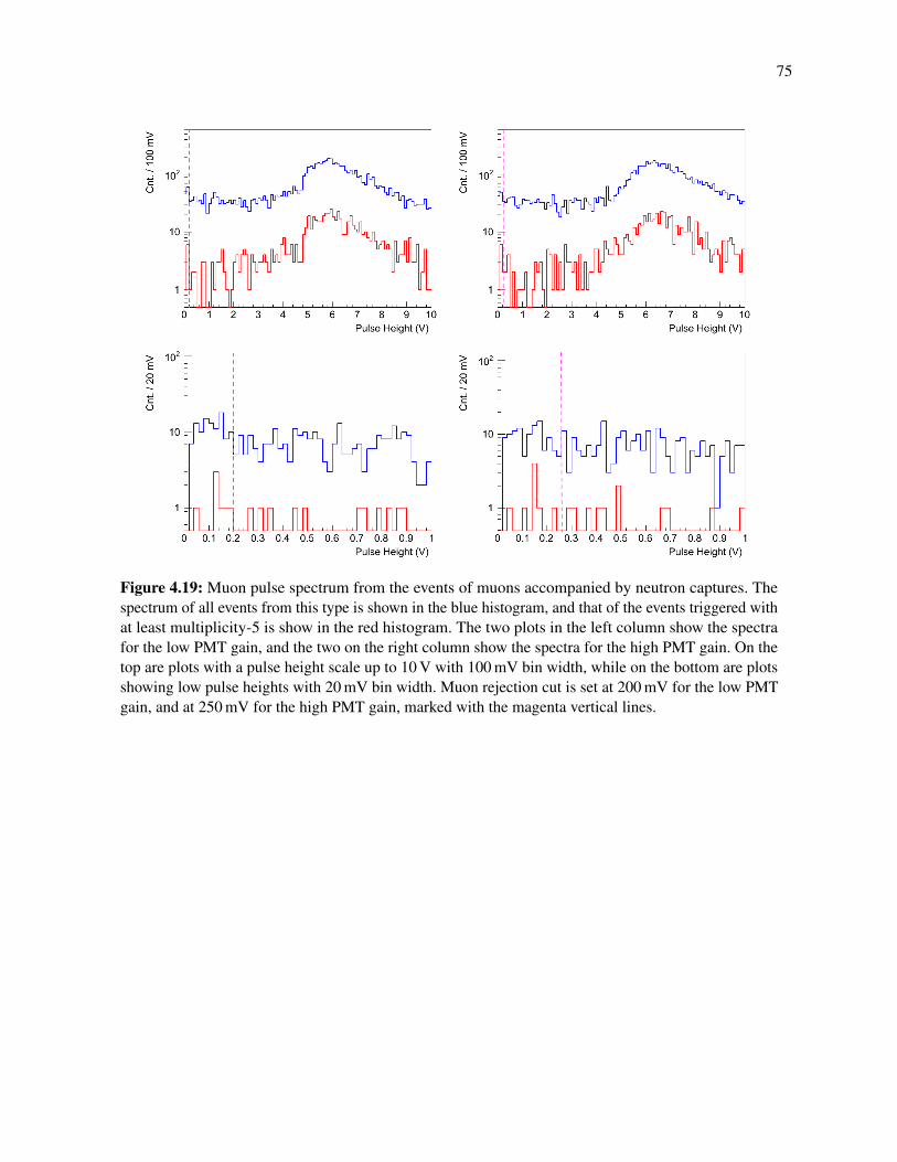
75

Figure 4.19: Muon pulse spectrum from the events of muons accompanied by neutron captures. Thespectrum of all events from this type is shown in the blue histogram, and that of the events triggered withat least multiplicity-5 is show in the red histogram. The two plots in the left column show the spectrafor the low PMT gain, and the two on the right column show the spectra for the high PMT gain. On thetop are plots with a pulse height scale up to 10 V with 100 mV bin width, while on the bottom are plotsshowing low pulse heights with 20 mV bin width. Muon rejection cut is set at 200 mV for the low PMTgain, and at 250 mV for the high PMT gain, marked with the magenta vertical lines.

76

previously surviving clipping muons for low PMT gain data, and tightening the cut to 250 mV is

expected to remove ∼ 14% previously surviving clipping muons for high PMT gain data.

Another muon problem in real data is the muons followed by afterpulses. Afterpulsing is led by

an initial pulse large enough to ionize the gas impurities significantly. A relative small pulse (down

to the neutron capture pulse region) is usually not expected to cause afterpulsing with 5 or more

coincident pulses to trigger. A tightened muon cut at 200 mV for low PMT gain data or 250 mV for

high PMT gain data would further secure the region of interest with few or no muon events falsely

selected.

4.2.5 Multiplicity Spectrum

With the multiplicity trigger threshold and the improved muon rejection cut applied, the selection

of candidate events can be determined. The MC truth analysis can help reveal how well the event

selection criteria work to include the expected signals, and how often backgrounds are falsely

included in the candidate set, which cannot be directly viewed in real data analysis. Table 4.2

summarizes the statistics of all types of events in MC truth on each selection requirement for both

the low PMT gain and the high PMT gain analyses. The first columns, “Hit”, show the number of

events making any PMT detected hit in the detector, the second columns, “M5”, list the number of

events having 5 or more pulses to meet the multiplicity trigger requirement, and the third columns,

“Selected”, list the number of events both having triggered and passed the muon rejection cut, which

requires the first two pulses be smaller than 200 mV for low PMT gain and 250 mV for high PMT

gain to make their efficiencies on neutron capture events both estimated as ∼ 96.7%. The numbers

of Hit and M5 events for low and high PMT gains are close within statistical uncertainty, while

the numbers of Selected events in types of fast neutrons and skewed fast neutrons for high PMT

gain are slightly greater than those for low PMT gain. The ratio of the Selected to the M5 events

appears much lower than 96.7%, which is due to the mis-tagging of the pulses from muons or

high-energy charge particles as neutron capture pulses. So the fast neutron events in M5 falsely

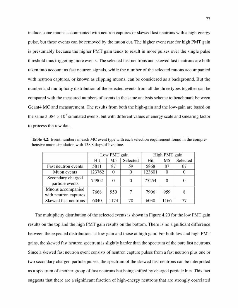
77

include some muons accompanied with neutron captures or skewed fast neutrons with a high-energy

pulse, but these events can be removed by the muon cut. The higher event rate for high PMT gain

is presumably because the higher PMT gain tends to result in more pulses over the single pulse

threshold thus triggering more events. The selected fast neutrons and skewed fast neutrons are both

taken into account as fast neutron signals, while the number of the selected muons accompanied

with neutron captures, or known as clipping muons, can be considered as a background. But the

number and multiplicity distribution of the selected events from all the three types together can be

compared with the measured numbers of events in the same analysis scheme to benchmark between

Geant4 MC and measurement. The results from both the high-gain and the low-gain are based on

the same 3.384×107 simulated events, but with different values of energy scale and smearing factor

to process the raw data.

Table 4.2: Event numbers in each MC event type with each selection requirement found in the compre-hensive muon simulation with 138.8 days of live time.

Low PMT gain High PMT gainHit M5 Selected Hit M5 Selected

Fast neutron events 5811 87 59 5868 87 67Muon events 123762 0 0 123601 0 0

Secondary chargedparticle events 74902 0 0 75254 0 0

Muons accompaniedwith neutron captures 7668 950 7 7906 959 8

Skewed fast neutrons 6040 1174 70 6030 1166 77

The multiplicity distribution of the selected events is shown in Figure 4.20 for the low PMT gain

results on the top and the high PMT gain results on the bottom. There is no significant difference

between the expected distributions at low gain and those at high gain. For both low and high PMT

gains, the skewed fast neutron spectrum is slightly harder than the spectrum of the pure fast neutrons.

Since a skewed fast neutron event consists of neutron capture pulses from a fast neutron plus one or

two secondary charged particle pulses, the spectrum of the skewed fast neutrons can be interpreted

as a spectrum of another group of fast neutrons but being shifted by charged particle hits. This fact

suggests that there are a significant fraction of high-energy neutrons that are strongly correlated

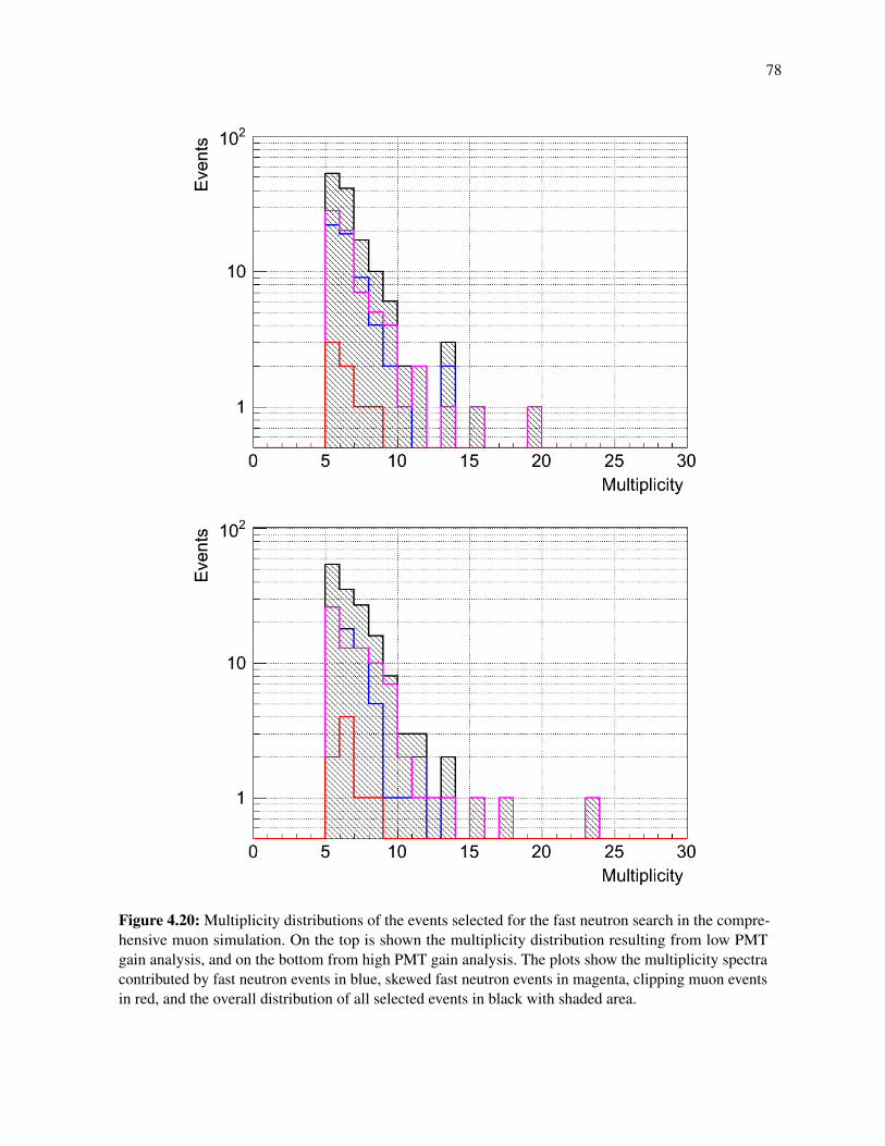
78

Figure 4.20: Multiplicity distributions of the events selected for the fast neutron search in the compre-hensive muon simulation. On the top is shown the multiplicity distribution resulting from low PMTgain analysis, and on the bottom from high PMT gain analysis. The plots show the multiplicity spectracontributed by fast neutron events in blue, skewed fast neutron events in magenta, clipping muon eventsin red, and the overall distribution of all selected events in black with shaded area.

79

with the primary muon between their incident angles, because many of the secondary particles

are from the muon emitted shower. The clipping muons are considered as an indistinguishable

background, which is∼ 5% of the selected events. The MC truth study has helped us understand the

content of the signals. However, since it is impossible to distinguish the three types of events with

measurement, the overall multiplicity distribution will be used to benchmark with the measured

multiplicity spectrum.

4.2.6 Neutron Flux Reconstruction

In addition to the results discussed above, an analysis on neutron flux may be performed to explore

the possibility of reconstructing the fast neutron flux from the measured event count and multiplicity

distribution.

Previous MC studies by M. Sweany [60] have indicated that the multiplicity has little dependence

on the energy of the incoming fast neutron, which is washed out by moderation and spallation in

the water. However, the trigger threshold at multiplicity 5 does play a role of energy threshold at

∼ 40−50MeV (shown in Figure 4.23 in [60]). Note that many incoming neutrons with energies

greater than 50 MeV may not trigger, but the triggered events have to be from the fast neutrons

above the effective energy threshold ∼ 40−50MeV. To reconstruct the flux of the fast neutrons

above threshold, it is necessary to investigate how the detected event count is related to the incoming

fast neutron flux.

Neutron flux is determined as the count of neutrons having passed a horizontal surface within a

unit of time and a unit of area. The neutron tracks recorded at the cavern ceiling, the top of the water

tanks, and the top of the bottom lead can be extracted to calculate the neutron fluxes accordingly.

The total count on each surface divided by the area of that surface and the live time of the simulation

is then the flux on that surface. In Figure 4.21, the differential fluxes of neutrons exiting the cavern

ceiling, through the top surfaces of the water tanks, and through the top surface of the bottom lead

80

as functions of neutron kinetic energy are plotted together. The fluxes through the tops of the tanks

and the bottom lead are only from counting the same neutrons recorded on the cavern ceiling and

walls. As expected, the fluxes at the cavern ceiling and the tops of the water tanks are close to each

other, except that the recording surface for the water tanks is under the top shielding lead, so that

the neutrons recorded are slightly attenuated by scattering and captures in the top lead. However,

the flux recorded through the top of the bottom lead is largely reduced compared with the flux

through the tops of the tanks for energies above 50 MeV, while the neutrons under 50 MeV have

been hugely increased. Moderation in the water causes the neutron energy to be reduced as it hits

the lead, and spallations in the water release low energy secondary neutrons. The flux through the

tops of water tanks will be used to study the detector acceptance.

In Figure 4.22, the spectrum of the primary neutron energies of the accepted events is normalized

by dividing by the live time and the area of the tops of the tanks to make an effective “detected

flux” (in solid line for overall events and colored lines for the three types of events) to be compared

with the incoming flux through the top surfaces of the water tanks (in dashed line). There is no

significant difference between the results from the low and the high PMT gain analyses shown in the

Figure. Besides the true high-energy neutrons (above 50 MeV), there are many low-energy neutrons

accepted in the analysis results.

A way to reveal more details is to plot 2-dimensional histograms of events with multiplicity vs.

neutron energy. Figure 4.23 plots these 2-dimensional histograms for fast neutron events on the

top, skewed fast neutron events in the middle, and clipping muon events on the bottom, with the

left column showing the results from low PMT gain and the right column from high PMT gain.

The histograms include only the events that pass muon cut, but keep the events with multiplicities

below 5. The events above multiplicity 5 are clearly distributed in two separate populations. For

the real high-energy neutrons, the multiplicity-5 trigger does make an effective energy threshold

at approximately 50 MeV, which is consistent with M. Sweany’s study. Another totally different

group of events that have multiplicities greater than 5 populate at very low energies, mostly below

81

Figure 4.21: Muon-induced neutron flux through three surfaces in the comprehensive muon simulation.In the black histogram is shown the neutron flux from the cavern ceiling, in the red histogram the fluxthrough the top surface of the water tanks, and in the blue histogram the flux through the top surface ofthe bottom lead. Only the neutrons directly incoming from cavern rock are included for counting thefluxes through the tank top and the bottom lead top.

82

Figure 4.22: Primary neutron energy spectrum of the accepted events, normalized with the tank topsurface area and MC live time, shown in black solid line for overall events and color lines for three typesof events. The total neutron flux through the top surface of the water tanks is shown in a dashed line tobe compared with the detected flux. The results for low and high PMT gains are shown on the top andbottom, respectively. For an event with more than one neutron hitting the top surface of the tanks, onlythe neutron with the highest energy is counted in the histograms.

83

10 MeV. The reason theses events can trigger is that they are multiple low energy neutrons incident

into the water tanks from the cavern rock in the same event. We may call these events “low-energy

neutron bundles”. These events are definitely not included in M. Sweany’s MC, in which only

mono-energetic neutron beams were shot into the north tank with one primary neutron per event.

For the clipping muon events, the main reason that the events can trigger is the muon-induced

neutrons in the lead stack, but the histograms show the energy of the primary neutron that happened

to fly from the cavern rock into the tanks. They are distributed at very low energy as well. The

low-energy neutron bundles emitted in rock and clipping muon events are both considered as

backgrounds for the detection of high-energy neutrons. The multiplicities of events with primary

neutron energies greater than and less than 50 MeV are compared in Figure 4.24. The real high-

energy neutrons do show a few events extending to higher multiplicities, but the difference between

the two multiplicity distributions is not significant enough to separate the two groups. We can extract

a fraction for neutrons above 50 MeV out of the overall accepted events. This fraction is estimated

to be (43±7)% for low PMT gain and (45±7)% for high PMT gain. Note there are a handful of

high-multiplicty events in Figure 4.24 but not in Figure 4.23. In theses events, the energies of the

primary neutrons are above 300 MeV.

Finally, to reconstruct a flux measurement of fast neutrons above 50 MeV, we can define the

gathering power of the detector as the quotient of the accepted event rate over the real high-energy

(> 50MeV) neutron flux,

G =Racc

F. (4.6)

This definition of gathering power is different from M. Sweany’s, but directly connects the measured

event rate of high-energy neutrons to the horizontal flux on the top of water tanks. According

to the statistics in Figure 4.22, the gathering power is estimated as (4.3±0.6)×103 cm2 for low

PMT gain and (5.0±0.6)×103 cm2 for high PMT gain. When analyzing real data, we can use the

estimated fraction of real high-energy neutrons first, then use the gathering power, to reconstruct a

flux measurement.

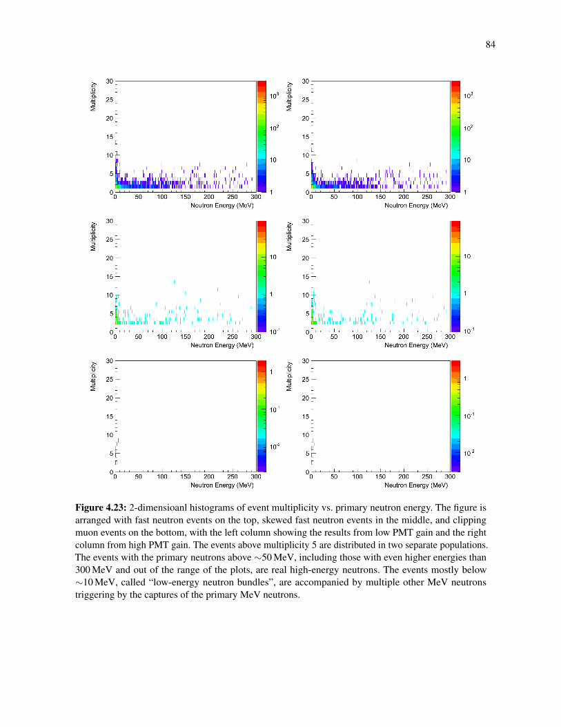
84

Figure 4.23: 2-dimensioanl histograms of event multiplicity vs. primary neutron energy. The figure isarranged with fast neutron events on the top, skewed fast neutron events in the middle, and clippingmuon events on the bottom, with the left column showing the results from low PMT gain and the rightcolumn from high PMT gain. The events above multiplicity 5 are distributed in two separate populations.The events with the primary neutrons above ∼50 MeV, including those with even higher energies than300 MeV and out of the range of the plots, are real high-energy neutrons. The events mostly below∼10 MeV, called “low-energy neutron bundles”, are accompanied by multiple other MeV neutronstriggering by the captures of the primary MeV neutrons.

85

Figure 4.24: The multiplicity distributions of the accepted events, split into the events of real high-energyneutrons (in blue) and the events of neutron bundles (in red), with the overall distribution (in black)plotted together. The real high-energy neutrons are selected as the incoming neutron energy greaterthan 50 MeV, and the neutron bundles as the highest neutron energy of the event less than 50 MeV. Thedistributions for low PMT gain is shown on the top plot, and the distributions for high PMT gain is onthe bottom.

Chapter 5

Fast Neutron Search Analysis for the Neutron

Multiplicity Meter Experiment

As mentioned in Chapter 3, there have been three periods of running for the fast neutron search,

with slightly different multiplicity trigger settings. The first fast neutron search run was taken with

a lower PMT gain, but the later two runs were taken after the PMT gain was raised and balanced.

The first fast neutron search run collected 158.2 live days of data, while the amount of data in the

second and third runs counts 169.2 days and 302.8 days of live time, respectively, making the total

630.2 days of live time. With the help of the better understood detector mechanism revealed in the

MC study in Chapter 4, the three data sets of fast neutron search have been analyzed to measure the

high-energy neutron flux at the Soudan Underground Laboratory, at a depth of ∼ 2000m.w.e, and

the high-energy neutron multiplicity spectrum, benchmarking the Geant4 MC.

In this chapter I present the analysis of the fast neutron search data. In addition to the muons

and muon-induced background particles, which are well understood in the Geant4 MC study, there

are gamma rays emitted by U/Th decays from ambient materials and the cavern rock. Most of the

gamma rays cannot trigger the detector since the trigger requires at least five coincident pulses in

the trigger window, but there is still a chance that five or more gammas are accidentally coincident

in the detector in a short time window. There are also pulses induced by electronic noise in the

86

87

neutron search data, which can affect the analysis and have not been studied in MC. In the analysis

of the neutron search data, a method based on the pulse height likelihood distribution has been

developed to discriminate gamma backgrounds, and data quality cuts were created to remove the

events with noise pulses. Finally, the multiplicity spectrum is extracted to compare with the result

from the Geant4 MC, and the data are also analyzed to make a measurement of the high-energy

neutron flux at the Soudan mine.

5.1 Pulse Height Likelihood Analysis

The types of events expected in the NMM have been introduced in Section 3.4.1. With muon

events and clipping muon with spallation neutrons well understood in the comprehensive MC study

and shown to be suppressed by the multiplicity trigger setting and muon rejection cut, the major

remaining background is the environmental gamma rays that accidentally fire the detector with

multiple coincident pulses in the trigger time window.

The rate of the multiple gamma events is determined mainly by the rate that gamma rays

arrive in coincidence. This gamma rate is measured with the U/Th background gamma exposure

data, which resulted in (330±3)Hz in the south tank and (367±3)Hz in the north tank in the

low-PMT-gain running period, and (412±4)Hz in the south tank and (433±4)Hz in the north

tank in the high-PMT-gain running period. The probability to have k coincident gamma pulses in

any trigger time window tTr conforms with the Poisson distribution, as

P(k;r tTr) =(r tTr)

k · e−r tTr

k!, (5.1)

with r the summed coincident gamma pulse rate in both tanks. To derive the rate of the gamma

events with a give multiplicity k, consider the occurance of k−1 gamma pulses in duration of time

88

tTr followed by one gamma pulse in time dt. The probability of an event defined as so is

Ik dt = P(k−1;r tTr) · r dt

=(r tTr)

k−1 · e−r tTr

(k−1)!r dt,

(5.2)

which gives the rate of gamma events with k gamma pulses,

Ik =(r tTr)

k−1 · e−r tTr

(k−1)!r. (5.3)

Taking the trigger time of the 1st fast neutron search run, tTr = 60µs, and the gamma rate to be

the sum over the two tanks measured for the low PMT period, r ≈ 697Hz, the rate of multiple

gamma events may be estimated for each multiplicity, namely the number of gamma pulses, k.

It is enlightening to compare the background gamma event rate with the estimated fast neutron

rate with respect to multiplicity. In Figure 5.1, the neutron multiplicity spectrum from the result

of the comprehensive muon simulation for low PMT gain is normalized with the live time of the

simulation to show the event rate of high-energy neutrons, plotted in the black histrogram. The

estimated multiple gamma rate is plotted in red. It is clear that the background gamma events are

dominant over the high-energy neutrons for low multiplicities, but the gamma rate plunges fast as

multiplicity increases. An event trigger set at 5 on multiplicity, indicated by the dashed magenta line,

can strongly suppress background gammas, though may still leave more multiple gamma events

than, or comparable with, the high-energy neutron events at multiplicity 5 and 6.

5.1.1 Pulse Height Likelihood Cut

A technique based on pulse height distributions has been developed to furthur seperate the remaining

multiple gamma events from high-energy neutrons. The spectrum of pulse heights (or “pulse

amplitudes”) of high-energy neutrons and that of background gammas form different distributions.

The high-energy neutron signal consists of multiple neutron capture pulses, which are directly

89

Figure 5.1: Comparison of background gammas and high-energy neutrons in event rate with respect tomultiplicity. The rate of multiple gamma events, in red circles and line, is estimated according to Poissondistribution with the input of measured single gamma rate in low PMT gain U/Th gamma exposure runs.The rate of high-energy neutrons as a function of multiplicity, in black histogram, is based on the resultsof the comprehensive muon simulation processed with low PMT gain parameters. The backgroundgammas are dominant over the high-energy neutron events at low multiplicities up to 5, but plunge fastas multiplicity increases. A trigger on multiplicity at 5 in the fast neutron search runs, labeled withthe magenta dashed line, efficiently suppresses most of background gammas. Removing the remainingmultiple gammas above the trigger threshold is a major task of the analysis in this chapter.

90

from ∼ 8MeV gamma cascades of the deexcitation of the capture products, while the background

gammas are from U/Th decays of energy spectrum with end point 2.6 MeV. The energy resolution

of the NMM detector is limited as shown in Section 4.1.3 with strong smearing over the features

of the original energy spectra. However, the detected pulse spectra of high-energy neutrons and

background gammas are still distinctive enough to develop a likelihood analysis. The comparison

of the pulse spectra of neutron captures and background gammas is shown in Figure 5.2, using

the neutron capture pulse spectrum (in blue) measured with the 252Cf calibration data and gamma

pulse spectrum (in red) measured with the U/Th background gamma exposure data (taken with

multiplicity-1 in 10 µs trigger). Gamma background (about 1-2% of the rate) was subtracted from

the pulse spectrum of the 252Cf calibration data to form the the neutron capture pulse spectrum. The

background gamma pulse spectrum peaks at ∼ 0.03V, and falls quickly, while the neutron capture

pulse spectrum peaks at ∼ 0.05V, and extends in a relative hard spectrum up to ∼ 0.28V.

By averaging the pulse height spectra of the south and north tanks, probability density functions

(PDFs) of neutron capture pulse height Pn(A) and background gamma pulse height Pg(A) can be

established for both low gain and high gain data, as functions of pulse height A. For an event of

M pulses with pulse heights A1, A2, ..., AM in fast neutron search data, the likelihood [71] that the

event is induced by a high-energy neutron (through neutron captures) is

n≡M

∏i=1

Pn(Ai) , (5.4)

while the likelihood for the event to be caused by M gammas is

g≡M

∏i=1

Pg(Ai) . (5.5)

n and g for an event may be compared to each other to indicate how likely the event is a fast neutron

or from background gammas. Previously, it was standard in this experiment to define a pulse height

91

Figure 5.2: Comparison of the pulse spectra of neutron captures and background gammas. The neutroncapture pulse spectrum (blue histogram) is measured with the 252Cf calibration data. Gamma pulsespectrum (red histogram) is measured with the U/Th background gamma exposure data. The backgroundgamma pulse spectrum peaks at ∼ 0.03V, and falls quickly, while the neutron capture pulse spectrumpeaks at ∼ 0.05V, and extends in a relative hard spectrum up to ∼ 0.28V.

92

likelihood fraction function

L≡ nn+g

, (5.6)

which can serve as a single estimator to tell how likely it is that an event is from a fast neutron or

from background gammas.

A demonstration of the distribution of L is shown in the gray histogram in Figure 5.3 for the

multiplicity 5 events from the 1st fast neutron search data. The greater and closer to 1 the value

of L, the more likely the event originated from a high-energy neutron. An L distribution of only

high-energy neutrons (in blue) and an L distribution of only multiple gamma events (in magenta)

can be drawn by MC sampling of fake neutron events from the fast neutron PDF n and the multiple

gamma PDF g, respectively. A preliminary method to seperate the high-energy neutrons and the

background gammas is to set a cut on L, say L > 0.99, labelled by the red vertical line. A χ2 fit with

the sum of the two components (in black) shows that the sum of the two components provides a

good fit to the data (χ2/ndf = 82.8/94). The MC sampling predicts that the L > 0.99 cut would

accept ∼ 68% high-energy neutron events, with ∼ 0.4 expected background gamma events, for the

event set of multiplicity 5.

5.1.2 Pulse Height Log-Likelihood Ratio (LLR) Fit

An analysis by setting a cut on L and estimating its efficiency would lead to extracting the original

number of signal events. Eventually, it is equivalent to just fitting the L distribution in data with the

modeled components of signal and background.

In addition, representing the data with L has its shortcomings. The most signal-like data, which

convey the most interesting information, are distributed around the high L region, particularly the

last bin in Figure 5.3. With these most informative data sorted in a single bin, a lot of important

information is lost. A better way of representing the likelihood is using a log-likelihood ratio

93

Figure 5.3: Distribution of “pulse-height likelihood” estimator L ≡ nn+g for the multiplicity 5 events

from the 1st fast neutron search data. The greater and closer to 1 the value of L, the more likely theevent is induced by a high-energy neutron. The less and closer to 0 the value of L, the more likely theevent is caused by background gammas. The expected distribution of L for high-energy neutrons only isshown in the blue histogram, and the expected distribution of L for multiple gammas only is shown inmagenta histogram. These expected distributions are generated by MC sampling of fake events fromthe neutron pulse height PDF Pn(A) and gamma pulse height PDF Pg(A) with 5 pulses per event andcalculating the L value from Eq. (5.7). The distributions are normalized by finding the best fit of theirsum (black histogram) to the data (gray histogram). The fit indicates that a cut of L > 0.99, labeled bythe red vertical line, would accept ∼ 68% high-energy neutron events, with ∼ 0.4 expected backgroundgamma events, from the multiplicity-5 data. The goodness-of-fit is χ2/nd f = 82.8/94, with p = 0.79.

94

(LLR) (with base 10 for a convenient correspondence to L) of the neutron likelihood to the gamma

likelihood

LLR≡ log10

(ng

). (5.7)

This representation will show the highly signal-like data in more detail, better revealing whether the

model provides a good fit. The LLR distribution of the multiplicity 5 events from the 1st fast neutron

search data is shown in Figure 5.4. Similar to the L distribution, the greater the value, the more

likely that an event is from a high-energy neutron. But an LLR value 2 approximately corresponds

to L = 0.99. The events in the last bin, from 0.99 − 1, of the L histogram have been extended to

a distribution with LLR > 2. The high peak around −2 represents the population of gamma-like

events.

5.1.3 Component Modeling for the LLR Fit

As discussed above, the components of the LLR distribution of the candidate events from fast

neutron search data include real fast neutron events as the signal and background gammas. For a

particular multiplicity M, they are the events with M neutron capture pulses and the events with M

gamma pulses. Naively speaking, there could also be the components for (M−1) neutrons with

1 gamma, (M−2) neutrons with 2 gammas, ..., and 1 neutron with (M−1) gammas in the LLR

distribution. To fit the LLR distribution, firstly, the component representing each case has to be

modeled. A pulse height induced by either a neutron capture or a background gamma is expected

to conform with the PDF of neutron captures, Pn(A), or the PDF of background gammas, Pg(A),

accordingly. Pulse heights can be sampled from the PDFs Pn(A) and Pg(A) with a Monte Carlo

method to form a pulse train for each of many events simulated, for each case of pulse compositions.

Then the LLR value may be calculated for all the sampled events of a given pulse composition to

form the LLR distribution of each case of pulse compositions. The pulse height PDFs for low and

95

Figure 5.4: Representation of neutron likelihood in log-likelihood ratio (LLR) log10(n

g

)for the

multiplicity-5 candidate events in the 1st fast neutron search data, with 1 LLR value difference per bin.The greater the LLR value, the more likely that an event is induced by a high-energy neutron. The largepopulation with a peak around -2 is formed by background gammas, while the events with LLR > 2 aremostly hign-energy neutron events. The cut L > 0.99 is approximately equivalent to cutting on LLR at 2.

96

high PMT gains are slightly different, so this process was done differently for the two gain settings

and applied appropriately to the different fast neutron search data sets, i.e. the model based on the

low PMT gain was used for the 1st fast neutron search, and the model based on high PMT gain was

used for the 2nd and 3rd fast neutron searches. Figure 5.5 shows the LLR component distributions

of multiplicity 5 for each case of pulse components, with the low gain distributions on the top and

the high gain on the bottom.

Given the Poisson distribution of the gamma pulse multiplicity with the measured gamma rate,

the rate of these coincidence with neutron capture and several gammas should be small. For a fast

neutron event with multiplicity (M−1), namely (M−1) neutron capture pulses in the 200 µs event

recording time, the rate of the fast neutron event being coincident with 1 gamma, in the 1st fast

neutron search data for example, is

R(M−1)n;1g =R(M−1)n ·P(1;697Hz ·200µs)

≈R(M−1)n ·0.121 ,(5.8)

with the notation P(k;r · t) = e−rt(rt)k/k! the Poisson distribution. In the 1st fast neutron search

data with 158 live days, the number of multiplicity 4 events is estimated by the compresensive muon

simulation as 137±12, which would result in ∼ 17 as the estimate of events with 4 neutrons and 1

gamma. This number is somewhat smaller than the simulation’s estimated multiplicity-5 events in

the 1st fast neutron search data, 62±8. Then, the rate of (M−2) neutron captures being coincident

with 2 gammas can be estimated as

R(M−2)n;2g =R(M−2)n ·P(2;697Hz ·200µs)

≈R(M−2)n ·0.00845 .(5.9)

With the number of multiplicity 3 events in the 1st fast neutron search data estimated as 273±15,

the number of events with 3 neutrons and 2 gammas is estimated as ∼ 2.3, which is smaller than the

uncertainty of estimated multiplicity 5 events and may be ignored. And the components of (M−3)

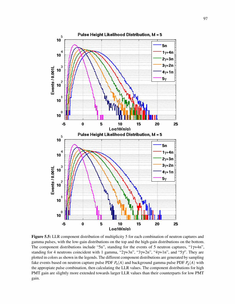
97

Figure 5.5: LLR component distribution of multiplicity 5 for each combination of neutron captures andgamma pulses, with the low-gain distributions on the top and the high-gain distributions on the bottom.The component distributions include “5n”, standing for the events of 5 neutron captures, “1γ+4n”,standing for 4 neutrons coincident with 1 gamma, “2γ+3n”, “3γ+2n”, “4γ+1n”, and “5γ”. They areplotted in colors as shown in the legends. The different component distributions are generated by samplingfake events based on neutron capture pulse PDF Pn(A) and background gamma pulse PDF Pg(A) withthe appropiate pulse combination, then calculating the LLR values. The component distributions for highPMT gain are slightly more extended towards larger LLR values than their counterparts for low PMTgain.

98

neutrons plus 3 gammas, etc. would be even smaller.

In summary, the model for the LLR fit includes the component of M neutron captures, the

component of (M− 1) neutron captures with 1 gamma, and the component of M gammas, but

ignoring the other possible pulse combinations, to fit the LLR distribution of multiplicity M events.

Furthermore, we may find the dependence of the (M−1)n+1g component on the Mn component,

and therefore constrain the fit further. The comprehensive muon simulation, although not necessarily

predicting the absolute multiplicity spectrum of high-energy neutrons accurately, should give a

reasonable estimation of the ratio of the event rates between two multiplicities. Thus, we can assume

A(M−1)n

AMn=NMC

(M−1)n

NMCMn

, (5.10)

where AMn denotes the amplitude of the M-neutron component in the LLR fit for the fast neutron

search data, and NMCMn denotes the number of M neutron events predicted by the MC. In the fast

neutron search data, some of the events with (M−1) neutron captures would be coincident with 1

gamma pulse and appear as multiplicity-M events. The probability of the coincidence is the Poisson

probability P1g of 1 gamma being present in 200 µs. Then we have

A(M−1)n+1g =A(M−1)n ·P1g . (5.11)

Combining the above two equations gives the dependence of the (M−1)n+1g amplitude on the Mn

amplitude,

A(M−1)n+1g = P1g ·NMC

(M−1)n

NMCMn

·AMn . (5.12)

Therefore, the fit for the LLR distribution of multiplicity M events includes three components, M

neutrons, (M−1) neutrons with 1 gamma, and M gammas. But only the amplitude of M neutrons,

AMn, and the amplitude of M gammas, AMg, are independent parameters.

99

The (M−1)n+1g events should be considered as signal, since most of the pulses are neutron

captures, signaling detection of fast neutrons. But their multiplicities are shifted by one, and

the estimates of these events should be counted as multiplicity (M−1) when reconstructing the

multiplicity spectrum.

5.2 Data Quality Cuts

The LLR fit of the fast neutron search data at first often resulted in rather bad fits for some

multiplicities. The gamma peak often shows discrepancy between the LLR distribution of fast

neutron data and the multi-gamma component in the model. Especially at the intermediate LLR

values (about −1≤M ≤ 2), the excess of events in the fast neutron search data over the model may

drive the amplitude of signal components up, and result in an overestimate of high-energy neutrons.

This issue is particularly severe in the 3rd fast neutron search data.

Unphysical events, such as those induced by electronic noise, are a common problem in particle

detection experiments, and are known to exist in the NMM as well. These noise pulse events may

compromise the LLR distribution, since they are neither neutron capture pulses nor background

gamma pulses. The afterpulsing induced by the muon events potentially leaking into the candidate

event set may also result in abnormal LLR values. Therefore, it is necessary to examine the data

quality over all the data sets of the fast neutron search, and develop data quality cuts to remove

unphysical events.

5.2.1 Muon Pulse and Afterpulsing with Mis-coincidence

In an examination of event waveforms among high-multiplicity fast neutron candidate events, some

dangerous events were spotted. They look like typical muon events with a large leading pulse and

many after-pulses, which should have been removed by the muon rejection cut. A example is shown

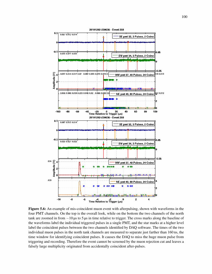
100

Figure 5.6: An example of mis-coincident muon event with afterpulsing, shown with waveforms in thefour PMT channels. On the top is the overall look, while on the bottom the two channels of the northtank are zoomed in from −10 µs to 5 µs in time relative to trigger. The cross marks along the baseline ofthe waveforms label the individual triggered pulses in a single PMT, and the star marks at a higher levellabel the coincident pulses between the two channels identified by DAQ software. The times of the twoindividual muon pulses in the north tank channels are measured to separate just farther than 160 ns, thetime window for identifying coincident pulses. It causes the DAQ to miss the huge muon pulse fromtriggering and recording. Therefore the event cannot be screened by the muon rejection cut and leaves afalsely large multiplicity originated from accidentally coincident after-pulses.

101

in Figure 5.6, with the overall look on the top and zoomed-in on the bottom. In the waveform plots,

the crosses along the baseline of the waveform mark the individual triggered pulses, while the stars

at a higher level label the identified coincident pulses. A closer look shows that the muon pulses in

the two north tank channels are not identified as a coincidence because their digitized pulse times

are just far enough to be out of the time window for identifying channel coincidence. Since the

leading large muon pulse is therefore not formally triggered and recorded, the event can sneak into

the candidate set without being caught by the muon cut on the first two pulses at 0.2 V or 0.25 V.

The remaining after-pulses make a very large number of coincident pulses just by accident, such as

24 in the example, potentially giving a very dangerous high-multiplicity false signal.

However, these sneaky mis-coincidence muon events are easy to remove. A cut on the individual

PMT pulses at 1 V works perfectly to clear this issue. This cut is high enough to avoid killing any

normal event of neutron captures, thus the efficiency can be considered 100%. This cut is included

as part of the muon cut for these data.

5.2.2 Removing Noise Pulses: Integral-Amplitude Ratio Cut

The electronic noise usually does not trigger pulses when the pulse threshold is properly set. But

there is still a chance for relatively large electronic noise to trigger and be recorded as pulses. The

shapes of the electronic noise pulses are usually very different than the normal photoelectron pulses

and appear much messier. Since the noise-triggered events are not physical, the noise pulses in the

two PMTs in a tank may only make coincident pulse pairs by accident, requiring the individual

pulse numbers in both channels to be much greater than the number of coincident pulse pairs. An

example of electronic noise event is shown in Figure 5.7, with the whole waveforms of four channels

on the top and zoomed-in at −20 µs to 20 µs on the bottom. In this event, the noise pulses happen

in the two PMTs of the north tank. The overall waveform on the top shows that there are many

individual noise pulses in the NW channel that cannot find counterparts in the NE channel to form

coincident pulses. So the 16 individual pulses in the NW and the 9 individual pulses in the NE give

102

only 5 coincident pulses for the north tank. With the zoomed-in waveforms shown on the bottom,

the pulses around 0 µs have very messy shapes, and the major pulse at ∼−1µs is much wider than

normal pulses, such as the pulse at ∼−5µs.

Based on the characteristics of the electronically noisy events discussed above, there may be two

major ways to remove them. One is to cut on the number of triggered pulses of individual channels

relative to the coincident pulse number. This method is found to be not very efficient at keeping

good events while cutting enough noisy events.

Another way is to exploit the characteristics of the pulse shapes of the noisy events. As shown in

the example event in Figure 5.7, the noisy events usually have some pulses with irregular shapes and

extra large widths. In reduced data format, there are both pulse amplitudes (pulse heights) and pulse

integrals recorded, though only amplitudes are used for the high-level analysis. The ratio of pulse

integral to pulse amplitude is proportional to pulse width, therefore may be used as an indicator to

tell if the pulse is induced by large electronic noise. To label an event, I choose to use the maximum

Integral-Amplitude Ratio (IAR) among all pulses of the event, and this quantity should form a

certain distribution among the normal events.

The 252Cf calibration data were taken to detect relatively intense neutron captures in short period

of time, so the probability for electronic noise events to happen in calibration data should be very

low. The IAR distributions of 252Cf calibration data for multiplicity 5 to 8 are shown as scatter

plots of IAR vs pulse height in Figure 5.8 for low-gain calibration and both Figures 5.9 and 5.10,

with blue dots for south tank events and orange dots for north tank events. The calibration events

distribute within a horizontal band which is wider for small pulse heights and narrower for large

pulse heights, and centered along IAR≈ 0.12. They are seldom found with IAR values greater than

2. For a comparison, the fast neutron search data are also plotted (with black dots) in Figure 5.8

for the 1st fast neutron search, Figure 5.9 for the 2nd, and Figure 5.10 for the 3rd. The PMT gains

of each fast neutron search data set corresponds to that of the 252Cf calibration data in each figure.

The events of the fast neutron search data in the figures have already passed the muon rejection cut.

103

Figure 5.7: An example of an electronic noise event, shown with waveforms in the four PMT channels.On the top is the overall look, while on the bottom the two channels of the north tank are zoomed infrom −20 µs to 20 µs in time relative to trigger. The noisy pulses appear in the north tank channels. Theindividual pulse numbers in the two channels of the north tank appear very unbalanced and there arerelatively few coincident pulses, shown in the overall waveform on the top figure. One of the majorpulses has a messy shape that is wider than usual, shown on the bottom zoomed-in waveform.

104

Most of these candidate events distribute in the band that aligns with the 252Cf neutron captures in

the 1st and 2nd fast neutron search data. A few outliers with large IAR values are considered as

electronic noise events. The 3rd fast neutron search seems to contain much more noise events, and

the distribution in Figure 5.10 indeed shows a vast distribution of high IAR events standing out of

the normal event band.

Figure 5.8: The scatter plots of pulse integral to amplitude ratio (IAR) vs pulse height of the 1st fastneutron search data and the low-gain run of 252Cf calibration. The IAR value for the event is that of thepulse with the maximum IAR in the event. The four plots show the data groups of multiplicity 5, 6, 7,and 8, respectively, as labeled on the top of each plot. The events of the 1st fast neutron search data, inblack dots, are already applied with another data quality cut and muon rejection cut. The events of 252Cfcalibration data are shown in blue dots for the south tank and orange dots for the north tank. The majorpopulation of fast neutron search events aligned well with the 252Cf calibration events in a band aroundIAR≈ 0.12 are considered as normal events, while a few events from the multiplicity 5 and 7 groupsin fast neutron search found with high IAR values are considered as electronic noise events. A cut ofIAR < 0.18, labeled with magenta lines, would just remove the noise events, without losing many goodevents.

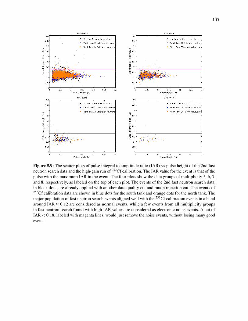
105

Figure 5.9: The scatter plots of pulse integral to amplitude ratio (IAR) vs pulse height of the 2nd fastneutron search data and the high-gain run of 252Cf calibration. The IAR value for the event is that of thepulse with the maximum IAR in the event. The four plots show the data groups of multiplicity 5, 6, 7,and 8, respectively, as labeled on the top of each plot. The events of the 2nd fast neutron search data,in black dots, are already applied with another data quality cut and muon rejection cut. The events of252Cf calibration data are shown in blue dots for the south tank and orange dots for the north tank. Themajor population of fast neutron search events aligned well with the 252Cf calibration events in a bandaround IAR ≈ 0.12 are considered as normal events, while a few events from all multiplicity groupsin fast neutron search found with high IAR values are considered as electronic noise events. A cut ofIAR < 0.18, labeled with magenta lines, would just remove the noise events, without losing many goodevents.

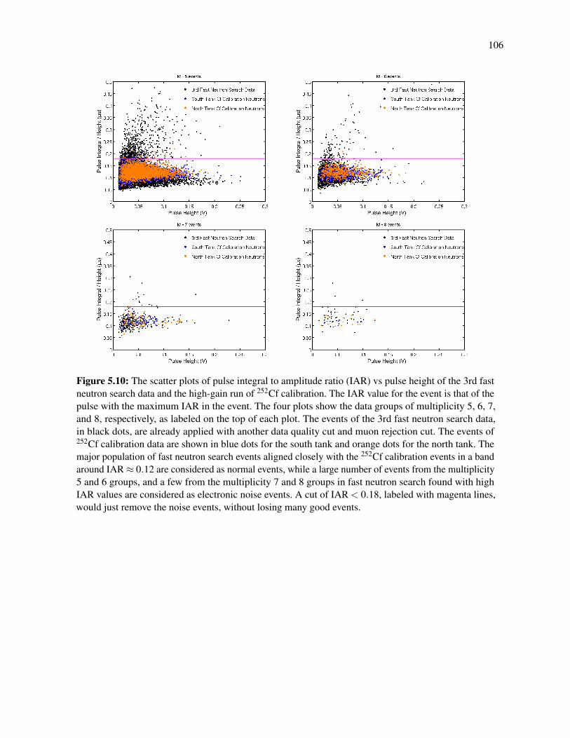
106

Figure 5.10: The scatter plots of pulse integral to amplitude ratio (IAR) vs pulse height of the 3rd fastneutron search data and the high-gain run of 252Cf calibration. The IAR value for the event is that of thepulse with the maximum IAR in the event. The four plots show the data groups of multiplicity 5, 6, 7,and 8, respectively, as labeled on the top of each plot. The events of the 3rd fast neutron search data,in black dots, are already applied with another data quality cut and muon rejection cut. The events of252Cf calibration data are shown in blue dots for the south tank and orange dots for the north tank. Themajor population of fast neutron search events aligned closely with the 252Cf calibration events in a bandaround IAR≈ 0.12 are considered as normal events, while a large number of events from the multiplicity5 and 6 groups, and a few from the multiplicity 7 and 8 groups in fast neutron search found with highIAR values are considered as electronic noise events. A cut of IAR < 0.18, labeled with magenta lines,would just remove the noise events, without losing many good events.

107

Figure 5.11: The histograms of pulse integral to amplitude ratio (IAR) for the 1st fast neutron searchdata and the low-gain run of 252Cf calibration. The IAR value for the event is that of the pulse withthe maximum IAR in the event. The four plots show the data groups of multiplicity 5, 6, 7, and 8,respectively, as labeled on the top of each plot. The events of the 1st fast neutron search data, in blackhistograms, are already applied with another data quality cut and muon rejection cut. The events of 252Cfcalibration data are shown in blue histograms for the south tank and orange histograms for the northtank. The majoraty of fast neutron search events populated closely with the 252Cf calibration events areconsidered as normal events, while a few events in fast neutron search found with high IAR values areconsidered as electronic noise events. The population of normal events in fast neutron search slightlymove towards high IAR values as multiplicity increases, since the IAR ratio of the event is selected asthe maximum IAR value from more pulses. A cut of IAR < 0.18, labeled with magenta lines, would justremove the noise events, without losing many good events.

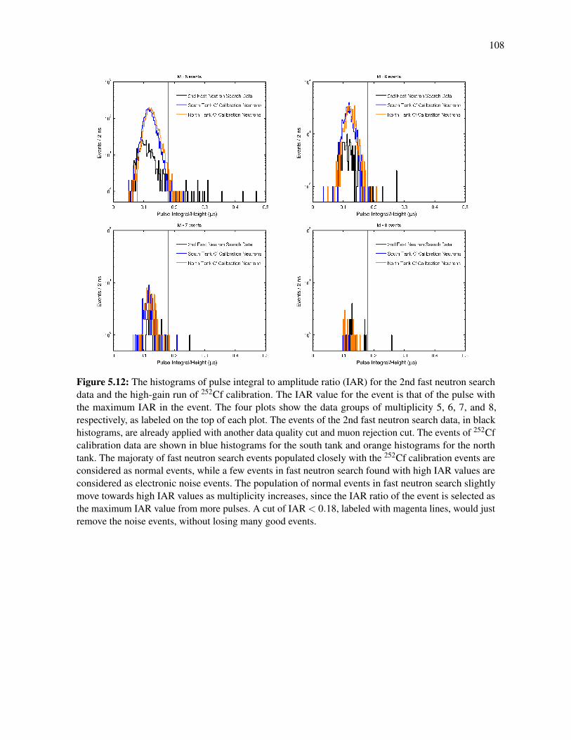
108

Figure 5.12: The histograms of pulse integral to amplitude ratio (IAR) for the 2nd fast neutron searchdata and the high-gain run of 252Cf calibration. The IAR value for the event is that of the pulse withthe maximum IAR in the event. The four plots show the data groups of multiplicity 5, 6, 7, and 8,respectively, as labeled on the top of each plot. The events of the 2nd fast neutron search data, in blackhistograms, are already applied with another data quality cut and muon rejection cut. The events of 252Cfcalibration data are shown in blue histograms for the south tank and orange histograms for the northtank. The majoraty of fast neutron search events populated closely with the 252Cf calibration events areconsidered as normal events, while a few events in fast neutron search found with high IAR values areconsidered as electronic noise events. The population of normal events in fast neutron search slightlymove towards high IAR values as multiplicity increases, since the IAR ratio of the event is selected asthe maximum IAR value from more pulses. A cut of IAR < 0.18, labeled with magenta lines, would justremove the noise events, without losing many good events.

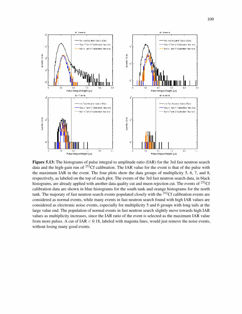
109

Figure 5.13: The histograms of pulse integral to amplitude ratio (IAR) for the 3rd fast neutron searchdata and the high-gain run of 252Cf calibration. The IAR value for the event is that of the pulse withthe maximum IAR in the event. The four plots show the data groups of multiplicity 5, 6, 7, and 8,respectively, as labeled on the top of each plot. The events of the 3rd fast neutron search data, in blackhistograms, are already applied with another data quality cut and muon rejection cut. The events of 252Cfcalibration data are shown in blue histograms for the south tank and orange histograms for the northtank. The majoraty of fast neutron search events populated closely with the 252Cf calibration events areconsidered as normal events, while many events in fast neutron search found with high IAR values areconsidered as electronic noise events, especially for multiplicity 5 and 6 groups with long tails at thelarge value end. The population of normal events in fast neutron search slightly move towards high IARvalues as multiplicity increases, since the IAR ratio of the event is selected as the maximum IAR valuefrom more pulses. A cut of IAR < 0.18, labeled with magenta lines, would just remove the noise events,without losing many good events.

110

Figure 5.14: Scatter plot of the IAR against multiplicity for the events of multiplicity 9 or greater havingpassed the muon rejection cut from all the three fast neutron searches. The IAR distribution is consistentwith the good 252Cf data.

To demonstrate the distribution of the IAR more clearly, the same comparisons are plotted as

histograms of IAR in Figures 5.11, 5.12, and 5.13 for the 1st, 2nd, and 3rd fast neutron search

data, respectively. It is found that the peak of the IAR of fast neutron candidate events sits at some

slightly smaller values than that of the calibration data for multiplicity 5, but moves towards higher

values as multiplicity increases. It is understandable. The IAR of an event is selected from the pulse

with the maximum IAR of the event. As multiplicity gets larger, the IAR is selected among more

pulses. Thus it is a natural tendency that IAR of fast neutron candidate events moves towards higher

values as multiplicity increases. It would not be wise to set too tight a cut, as it could falsely remove

too many good events for high multiplicities. A cut of IAR < 0.18 is tight enough to remove all

the noisy events that are clearly outliers in the long tails of the distributions, but not so tight that it

reduces efficiency appreciably for the main peak of good events. Given the tendency of the peak

of good events to move towards higher values for larger multiplicities, it is better not to apply the

111

cut to events of 9 and more multiplicities. To check if there are non-physical events of multiplicity

9 or greater, the IAR distribution of these events were examined. Figure 5.14 is a scatter plot of

the IAR against multiplicity for the events of multiplicity 9 or greater having passed the muon

rejection cut from all fast neutron search data. It is clear shown that the IAR distribution of these

high-multiplicity events is consistent with the good 252Cf data. I also checked the raw-waveform

traces of these events, and found no peculiar events.

Although the calibration data may not perfectly represent the distribution of IAR for high-energy

neutrons, they are still the best sample we can trust, without significant conatamination of noise

events and background gammas. Therefore, we use the 252Cf neutron calibration data to measure the

efficiency of the IAR cut. Assuming all 252Cf events are physical events, with the cut of IAR < 0.18,

the measured efficiency, i.e. the acceptance of good neutron capture events, is shown in Figure 5.15

at multiplicity 5 to 8. The efficiency for low-gain data is shown on the top, while for high-gain

data is on the bottom. The measurements based on the south tank events are plotted in blue circle

and error bar, while the measurements based on the north tank events are in red. In black is shown

the measurement using data over both tanks for each multiplicity. As the efficiency approximate

keeps constant through these multiplicities, it is good enough to quote a constant cut efficiency.

The efficiency of the IAR cut is then measured with the multiplicity 5 through 8 252Cf, to be

0.9959+0.0008−0.0009 for low-gain data and 0.9952+0.0008

−0.0009 for high-gain data, shown in Figure 5.15.

112

Figure 5.15: The efficiency of the data quality cut of IAR < 0.18, defined as the acceptance fractionfor good 252Cf calibration events. On the top is measured with the low-gain 252Cf calibration run, andon the bottom is measured with the high-gain 252Cf calibration run. The circles with error bars showthe efficiencies measured with multiplicity 5 to 8 individually, with blue for south tank data, red fornorth tank data, and black for the overall measurement combining both tanks. The change in efficiencyas multiplicity increases is not significant, so it is reasonable to treat the efficiency as a constant overmultiplicity 5 to 8. The measurements using the overall data including multiplicity 5 to 8 suggest theefficiency to be 0.9959+0.0008

−0.0009 for low-gain data and 0.9952+0.0008−0.0009 for high-gain data, marked with

magenta solid lines, with error bars, almost directly on top of the average, in magenta dashed lines. Theblack dashed line marks one.

113

5.3 Results of Log-Likelihood-Ratio (LLR) Fit

Based on the model of three components discussed in section 5.1, χ2 fits are performed for data

collection of each multiplicity in each fast neutron search data set, with the muon and IAR data

quality cuts discussed in section 5.2 applied. In this section, I present the results of the LLR fit for

each multiplicity case for all the fast neutron search data sets, in Figures 5.16 through 5.32. As

described in Section 5.1.3, each fit has only two free parameters: the number of photon events, and

the the number of all-neutron events, with the number of 1g events given by Eq. (5.12). In each plot,

the LLR distribution of the fast neutron search data is in the gray shaded histogram; for the events

of multiplicity M, the signal component Mn is shown in blue histogram, the signal component

(M−1)n+1g in orange, the background component Mg in red, and the fit function, i.e. the sum of

above three, is black. The LLR value range for the fit is shown as in between two dashed magenta

lines.

With the data quality cuts added to the analysis, the candidate events give LLR distributions

more consistent with the model distributions in most cases. But for multiplicity 5 events in the 1st

fast neutron search (Figure 5.16), and multiplicity 5 and 6 events in the 3rd fast neutron search

(Figure 5.27 and Figure 5.28), the intermediate LLR distribution still shows a large excess over

the fit model. Tighter cuts, or the cuts based on pulse numbers on individual channels do not

preferentially remove events in this regions, suggesting that these events are not unphysical, noise

events. Another possible explaination of the excess is that the true LLR distribution of gamma events

has a harder spectrum than expected at the intermediate values, as may occur if the pulse-height

distribution of gammas is harder than indicated by U/Th calibration runs. There were only a few

calibration runs and U/Th gamma exposure runs, not covering the whole period of fast neutron

searches. It is possible that the background gamma pulse spectrum drifted due to PMT gain changing

or other unknown reasons, so the likelihood model does not reflect the exact distribution. Given the

circumstance, the best we can do is to keep using the current data quality cuts, and do the LLR fit

114

in a partial range, with which the fit performs well, but avoid the intermediate region. The partial

range fits of the LLR distribution are performed for multiplicity 5 and 6 events in the 1st and the

3rd fast neutron search data, shown in Figure 5.16, Figure 5.17, Figure 5.27, and Figure 5.28. The

fit ranges are marked with the dashed magenta lines, with the active value ranges for fitting between

the first and second lines, and also between the third and fourth lines. With this treatment, the fits

are in good agreement with the data in the gamma peak region and the most signal-like region. The

total numbers of events estimated by the fit function show reasonably close to the total number in in

data. The signal components, Mn and (M−1)n+1g should then give good estimates of the number

of fast neutron events.

Beyond multiplicity 6 in the fast neutron search data, the statistics in each multiplicity appears

too low to bin into every 1 LLR difference and still get a meaningful distribution. For the multiplicity

7 to 10, we choose to use bins of 3 LLR difference. In the 2nd fast neutron search, the events of

multiplicity 6 may be binned with 1 LLR difference bins, but with 3 LLR difference bins it is easier

to see the agreement by eye with the statistical fluctuation being smeared. So I use the wider bins

for this case as well. Note that there is no multiplicity 5 data set in the 2nd fast neutron search data,

since the 2nd fast neutron search was run with trigger at multiplicity 6 in 70 µs.

For the choice of fitting range, it is generally good to include all candidate events. Usually it

does not matter whether to include one more bin with zero counts. For some cases, it is crucial to

include the zero-count bin, where the LLR values are the typical values that background gammas

occupy. One instance is multiplicity 8 in the 1st fast neutron search, shown in Figure 5.19. If the -6

to -3 bin with zero counts were not included in the fit, the background gamma component in the -3

to 0 bin would rise up to match the data, making gamma component in the -6 to -3 bin falsely high.

This would give a poor estimate of total background gamma rate, and might potentially be harmful

for signal rate extraction as well.

As the multiplicity increases, the chance to include background gamma events in the candidate

set goes extremely low, as for multiplicity 8 to 10 in the 1st and 2nd fast neutron search data, or it

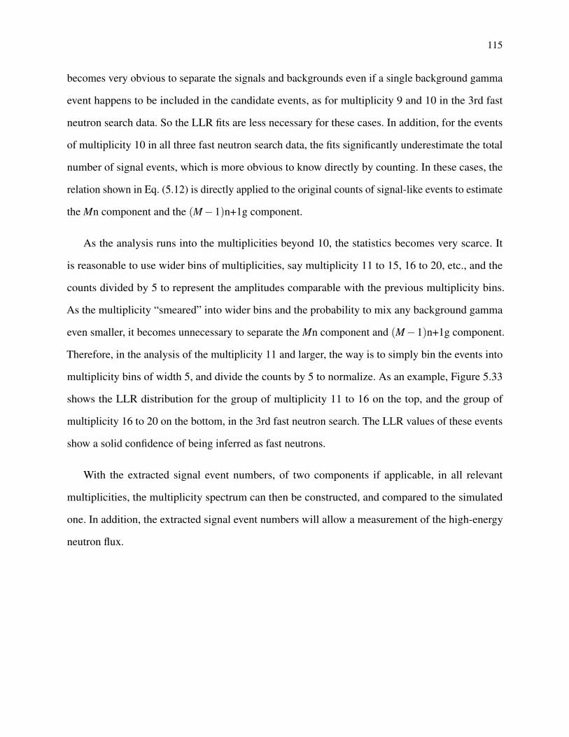
115

becomes very obvious to separate the signals and backgrounds even if a single background gamma

event happens to be included in the candidate events, as for multiplicity 9 and 10 in the 3rd fast

neutron search data. So the LLR fits are less necessary for these cases. In addition, for the events

of multiplicity 10 in all three fast neutron search data, the fits significantly underestimate the total

number of signal events, which is more obvious to know directly by counting. In these cases, the

relation shown in Eq. (5.12) is directly applied to the original counts of signal-like events to estimate

the Mn component and the (M−1)n+1g component.

As the analysis runs into the multiplicities beyond 10, the statistics becomes very scarce. It

is reasonable to use wider bins of multiplicities, say multiplicity 11 to 15, 16 to 20, etc., and the

counts divided by 5 to represent the amplitudes comparable with the previous multiplicity bins.

As the multiplicity “smeared” into wider bins and the probability to mix any background gamma

even smaller, it becomes unnecessary to separate the Mn component and (M−1)n+1g component.

Therefore, in the analysis of the multiplicity 11 and larger, the way is to simply bin the events into

multiplicity bins of width 5, and divide the counts by 5 to normalize. As an example, Figure 5.33

shows the LLR distribution for the group of multiplicity 11 to 16 on the top, and the group of

multiplicity 16 to 20 on the bottom, in the 3rd fast neutron search. The LLR values of these events

show a solid confidence of being inferred as fast neutrons.

With the extracted signal event numbers, of two components if applicable, in all relevant

multiplicities, the multiplicity spectrum can then be constructed, and compared to the simulated

one. In addition, the extracted signal event numbers will allow a measurement of the high-energy

neutron flux.

116

Figure 5.16: Least-squares fit of the LLR distribution for the multiplicity 5 events in the 1st fast neutronsearch data with a model composed of signal components 5n (blue), multiplicity-shifted signal component4n+1g (orange), and background gamma component 5g (red). The candidate events, shown in the grayhistogram, are binned per 1 LLR difference. The fit is performed in a partial range, from -5 to -1, andfrom 3 to 9, labeled as in between the first two magenta lines and in between the third and fourthmagenta lines, respectively. The resulted fit function, shown in the black histogram, is the sum of thethree components, with amplitudes of 5n and 5g as the two free parameters, while the amplitude of the4n+1g component dependent on that of 5n according to Eq. (5.12). The goodness-of-fit is tested to beχ2/nd f = 2.36/8, with p = 0.97.

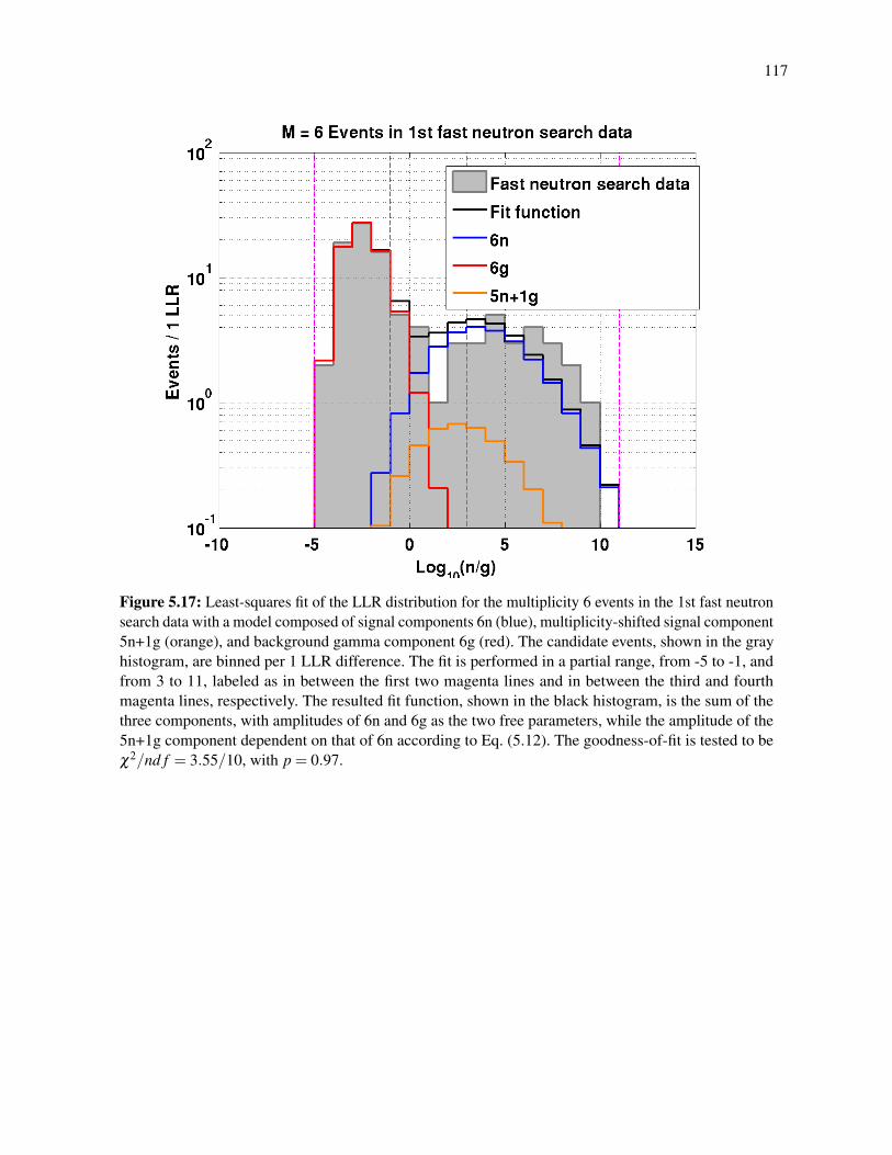
117

Figure 5.17: Least-squares fit of the LLR distribution for the multiplicity 6 events in the 1st fast neutronsearch data with a model composed of signal components 6n (blue), multiplicity-shifted signal component5n+1g (orange), and background gamma component 6g (red). The candidate events, shown in the grayhistogram, are binned per 1 LLR difference. The fit is performed in a partial range, from -5 to -1, andfrom 3 to 11, labeled as in between the first two magenta lines and in between the third and fourthmagenta lines, respectively. The resulted fit function, shown in the black histogram, is the sum of thethree components, with amplitudes of 6n and 6g as the two free parameters, while the amplitude of the5n+1g component dependent on that of 6n according to Eq. (5.12). The goodness-of-fit is tested to beχ2/nd f = 3.55/10, with p = 0.97.

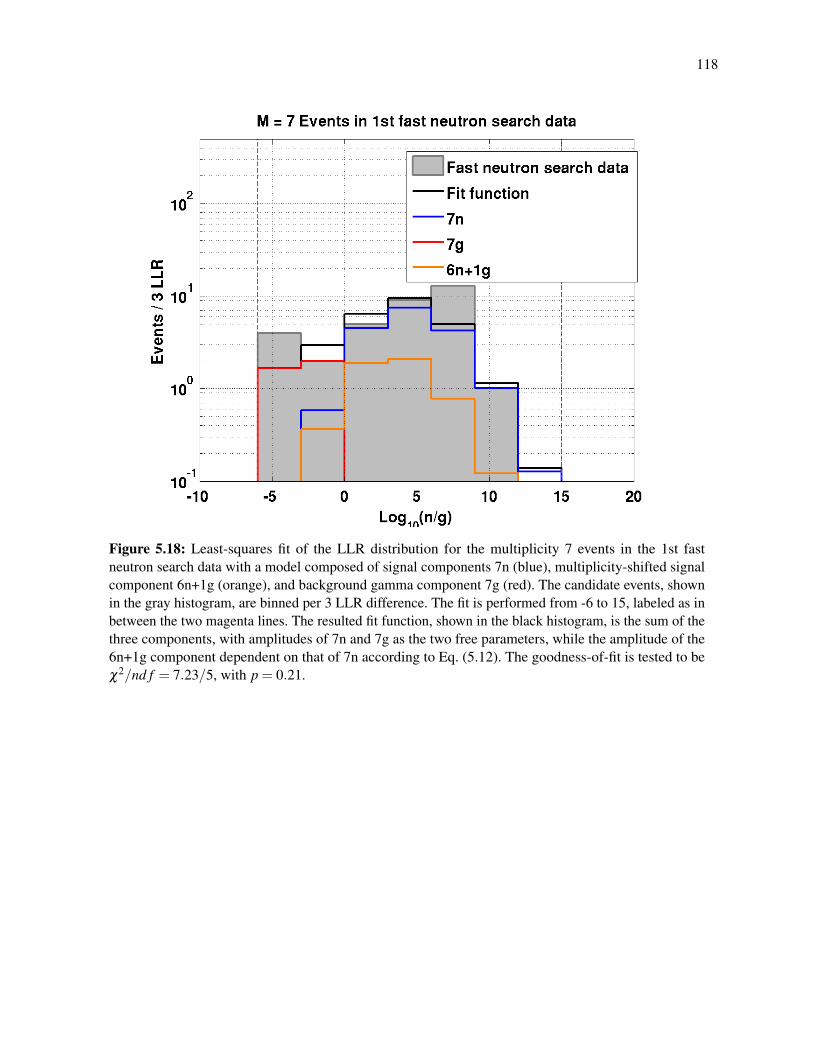
118

Figure 5.18: Least-squares fit of the LLR distribution for the multiplicity 7 events in the 1st fastneutron search data with a model composed of signal components 7n (blue), multiplicity-shifted signalcomponent 6n+1g (orange), and background gamma component 7g (red). The candidate events, shownin the gray histogram, are binned per 3 LLR difference. The fit is performed from -6 to 15, labeled as inbetween the two magenta lines. The resulted fit function, shown in the black histogram, is the sum of thethree components, with amplitudes of 7n and 7g as the two free parameters, while the amplitude of the6n+1g component dependent on that of 7n according to Eq. (5.12). The goodness-of-fit is tested to beχ2/nd f = 7.23/5, with p = 0.21.

119

Figure 5.19: Least-squares fit of the LLR distribution for the multiplicity 8 events in the 1st fast neutronsearch data with a model composed of signal components 8n (blue), multiplicity-shifted signal component7n+1g (orange), and background gamma component 8g (red). The candidate events, shown in the grayhistogram, are binned per 3 LLR difference. The fit is performed from -6 to 15, labeled as in betweenthe two magenta lines. The first empty bin is necessary to be included to constrain 8g component. Theresulted fit function, shown in the black histogram, is the sum of the three components, with amplitudesof 8n and 8g as the two free parameters, while the amplitude of the 7n+1g component dependent on thatof 8n according to Eq. (5.12). The goodness-of-fit is tested to be χ2/nd f = 2.22/5, with p = 0.82.

120

Figure 5.20: Least-squares fit of the LLR distribution for the multiplicity 9 events in the 1st fast neutronsearch data with a model composed of signal components 9n (blue), multiplicity-shifted signal component8n+1g (orange), and background gamma component 9g (red). The candidate events, shown in the grayhistogram, are binned per 3 LLR difference. The fit is performed from -3 to 15, labeled as in betweenthe two magenta lines. The first empty bin is necessary to be included to constrain 9g component. Theresulted fit function, shown in the black histogram, is the sum of the three components, with amplitudesof 9n and 9g as the two free parameters, while the amplitude of the 8n+1g component dependent on thatof 9n according to Eq. (5.12). The goodness-of-fit is tested to be χ2/nd f = 2.06/4, with p = 0.72.

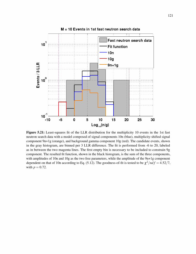
121

Figure 5.21: Least-squares fit of the LLR distribution for the multiplicity 10 events in the 1st fastneutron search data with a model composed of signal components 10n (blue), multiplicity-shifted signalcomponent 9n+1g (orange), and background gamma component 10g (red). The candidate events, shownin the gray histogram, are binned per 3 LLR difference. The fit is performed from -6 to 20, labeledas in between the two magenta lines. The first empty bin is necessary to be included to constrain 9gcomponent. The resulted fit function, shown in the black histogram, is the sum of the three components,with amplitudes of 10n and 10g as the two free parameters, while the amplitude of the 9n+1g componentdependent on that of 10n according to Eq. (5.12). The goodness-of-fit is tested to be χ2/nd f = 4.52/7,with p = 0.72.

122

Figure 5.22: Least-squares fit of the LLR distribution for the multiplicity 6 events in the 2nd fastneutron search data with a model composed of signal components 6n (blue), multiplicity-shifted signalcomponent 5n+1g (orange), and background gamma component 6g (red). The candidate events, shownin the gray histogram, are binned per 3 LLR difference. The fit is performed from -6 to 15, labeled as inbetween the first two magenta lines. The resulted fit function, shown in the black histogram, is the sumof the three components, with amplitudes of 6n and 6g as the two free parameters, while the amplitudeof the 5n+1g component dependent on that of 6n according to Eq. (5.12). The goodness-of-fit is tested tobe χ2/nd f = 1.98/5, with p = 0.85.

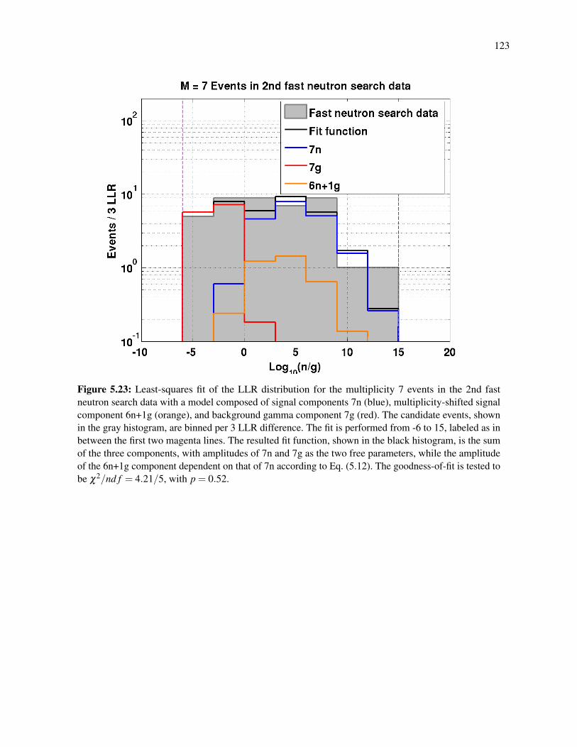
123

Figure 5.23: Least-squares fit of the LLR distribution for the multiplicity 7 events in the 2nd fastneutron search data with a model composed of signal components 7n (blue), multiplicity-shifted signalcomponent 6n+1g (orange), and background gamma component 7g (red). The candidate events, shownin the gray histogram, are binned per 3 LLR difference. The fit is performed from -6 to 15, labeled as inbetween the first two magenta lines. The resulted fit function, shown in the black histogram, is the sumof the three components, with amplitudes of 7n and 7g as the two free parameters, while the amplitudeof the 6n+1g component dependent on that of 7n according to Eq. (5.12). The goodness-of-fit is tested tobe χ2/nd f = 4.21/5, with p = 0.52.

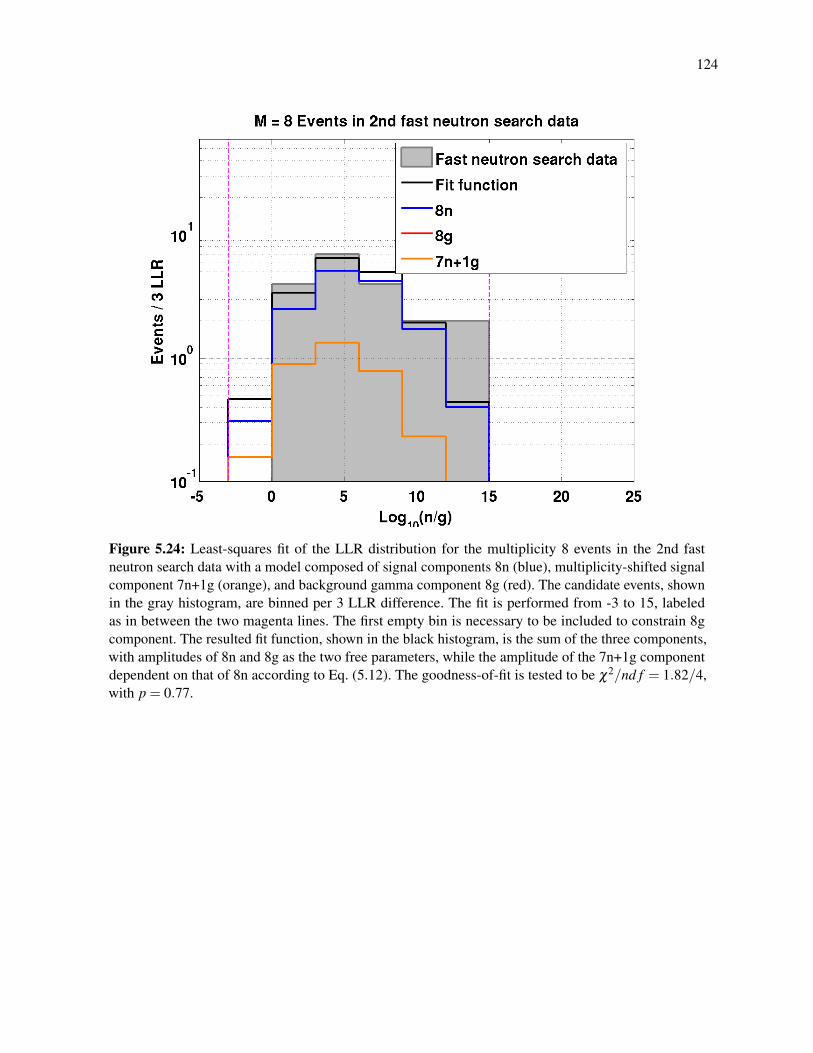
124

Figure 5.24: Least-squares fit of the LLR distribution for the multiplicity 8 events in the 2nd fastneutron search data with a model composed of signal components 8n (blue), multiplicity-shifted signalcomponent 7n+1g (orange), and background gamma component 8g (red). The candidate events, shownin the gray histogram, are binned per 3 LLR difference. The fit is performed from -3 to 15, labeledas in between the two magenta lines. The first empty bin is necessary to be included to constrain 8gcomponent. The resulted fit function, shown in the black histogram, is the sum of the three components,with amplitudes of 8n and 8g as the two free parameters, while the amplitude of the 7n+1g componentdependent on that of 8n according to Eq. (5.12). The goodness-of-fit is tested to be χ2/nd f = 1.82/4,with p = 0.77.

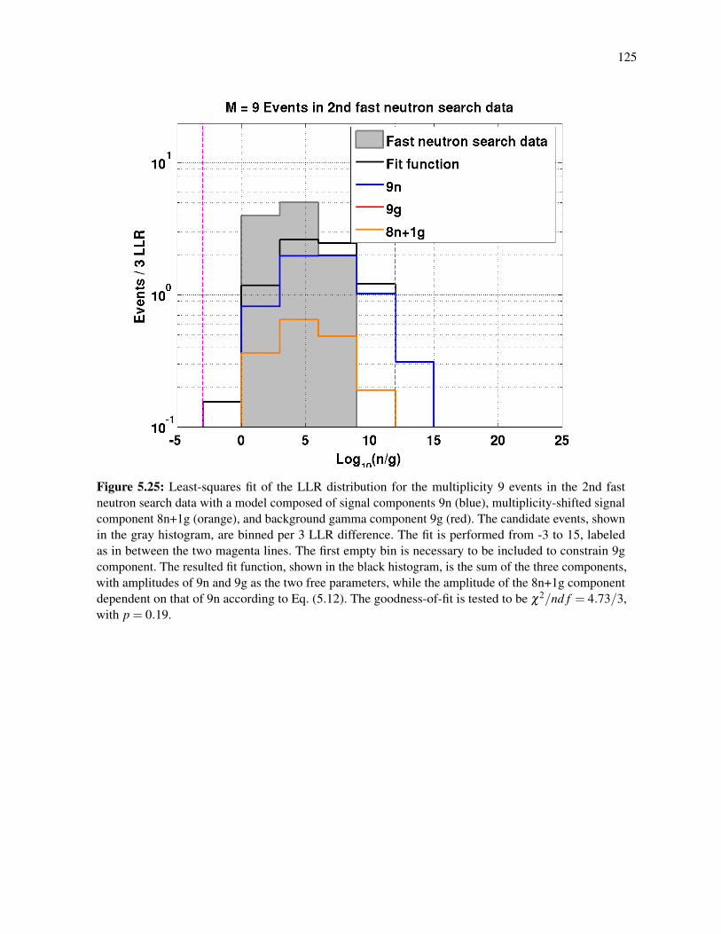
125

Figure 5.25: Least-squares fit of the LLR distribution for the multiplicity 9 events in the 2nd fastneutron search data with a model composed of signal components 9n (blue), multiplicity-shifted signalcomponent 8n+1g (orange), and background gamma component 9g (red). The candidate events, shownin the gray histogram, are binned per 3 LLR difference. The fit is performed from -3 to 15, labeledas in between the two magenta lines. The first empty bin is necessary to be included to constrain 9gcomponent. The resulted fit function, shown in the black histogram, is the sum of the three components,with amplitudes of 9n and 9g as the two free parameters, while the amplitude of the 8n+1g componentdependent on that of 9n according to Eq. (5.12). The goodness-of-fit is tested to be χ2/nd f = 4.73/3,with p = 0.19.

126

Figure 5.26: Least-squares fit of the LLR distribution for the multiplicity 10 events in the 2nd fastneutron search data with a model composed of signal components 10n (blue), multiplicity-shifted signalcomponent 9n+1g (orange), and background gamma component 10g (red). The candidate events, shownin the gray histogram, are binned per 3 LLR difference. The fit is performed from 0 to 15, labeled asin between the two magenta lines. The first empty bin is necessary to be included to constrain 10gcomponent. The resulted fit function, shown in the black histogram, is the sum of the three components,with amplitudes of 10n and 10g as the two free parameters, while the amplitude of the 9n+1g componentdependent on that of 10n according to Eq. (5.12). The goodness-of-fit is tested to be χ2/nd f = 1.54/3,with p = 0.67.

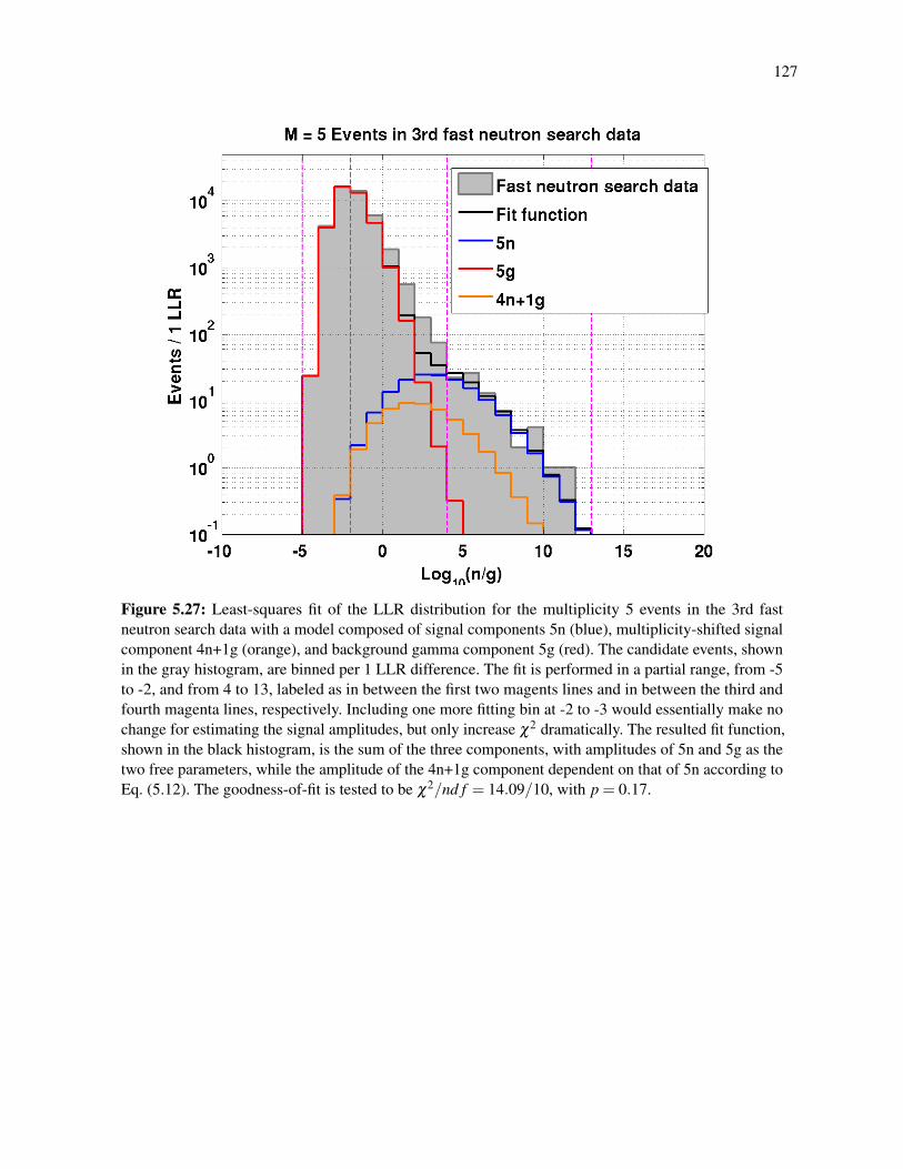
127

Figure 5.27: Least-squares fit of the LLR distribution for the multiplicity 5 events in the 3rd fastneutron search data with a model composed of signal components 5n (blue), multiplicity-shifted signalcomponent 4n+1g (orange), and background gamma component 5g (red). The candidate events, shownin the gray histogram, are binned per 1 LLR difference. The fit is performed in a partial range, from -5to -2, and from 4 to 13, labeled as in between the first two magents lines and in between the third andfourth magenta lines, respectively. Including one more fitting bin at -2 to -3 would essentially make nochange for estimating the signal amplitudes, but only increase χ2 dramatically. The resulted fit function,shown in the black histogram, is the sum of the three components, with amplitudes of 5n and 5g as thetwo free parameters, while the amplitude of the 4n+1g component dependent on that of 5n according toEq. (5.12). The goodness-of-fit is tested to be χ2/nd f = 14.09/10, with p = 0.17.

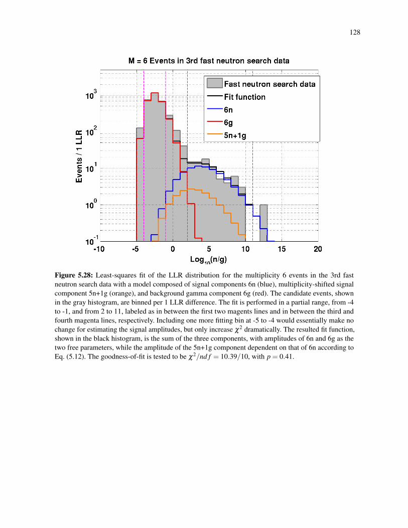
128

Figure 5.28: Least-squares fit of the LLR distribution for the multiplicity 6 events in the 3rd fastneutron search data with a model composed of signal components 6n (blue), multiplicity-shifted signalcomponent 5n+1g (orange), and background gamma component 6g (red). The candidate events, shownin the gray histogram, are binned per 1 LLR difference. The fit is performed in a partial range, from -4to -1, and from 2 to 11, labeled as in between the first two magents lines and in between the third andfourth magenta lines, respectively. Including one more fitting bin at -5 to -4 would essentially make nochange for estimating the signal amplitudes, but only increase χ2 dramatically. The resulted fit function,shown in the black histogram, is the sum of the three components, with amplitudes of 6n and 6g as thetwo free parameters, while the amplitude of the 5n+1g component dependent on that of 6n according toEq. (5.12). The goodness-of-fit is tested to be χ2/nd f = 10.39/10, with p = 0.41.

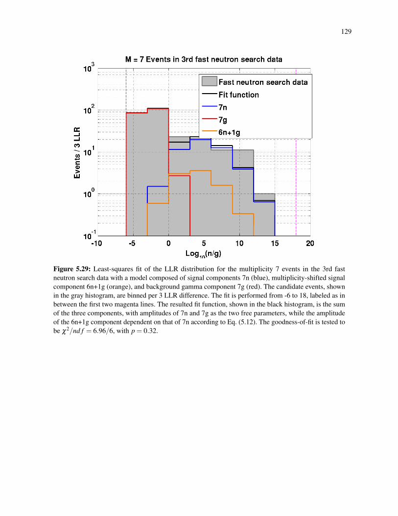
129

Figure 5.29: Least-squares fit of the LLR distribution for the multiplicity 7 events in the 3rd fastneutron search data with a model composed of signal components 7n (blue), multiplicity-shifted signalcomponent 6n+1g (orange), and background gamma component 7g (red). The candidate events, shownin the gray histogram, are binned per 3 LLR difference. The fit is performed from -6 to 18, labeled as inbetween the first two magenta lines. The resulted fit function, shown in the black histogram, is the sumof the three components, with amplitudes of 7n and 7g as the two free parameters, while the amplitudeof the 6n+1g component dependent on that of 7n according to Eq. (5.12). The goodness-of-fit is tested tobe χ2/nd f = 6.96/6, with p = 0.32.

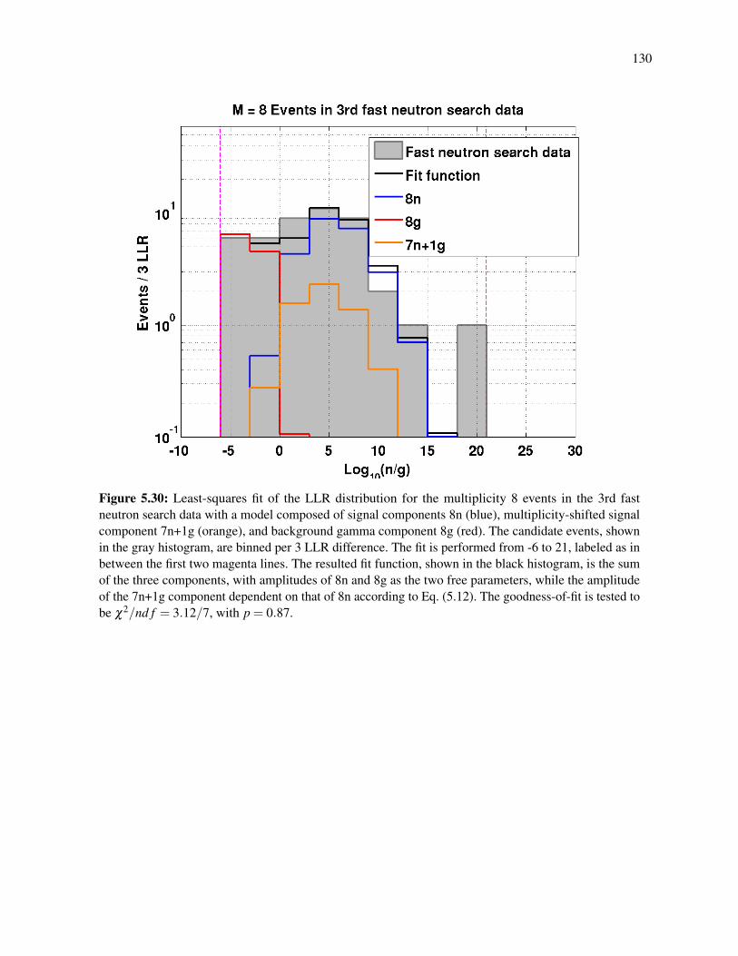
130


131


132

Figure 5.32: Least-squares fit of the LLR distribution for the multiplicity 10 events in the 3rd fastneutron search data with a model composed of signal components 10n (blue), multiplicity-shifted signalcomponent 8n+1g (orange), and background gamma component 10g (red). The candidate events, shownin the gray histogram, are binned per 3 LLR difference. The fit is performed from -6 to 18, labeled as inbetween the first two magenta lines. The resulted fit function, shown in the black histogram, is the sumof the three components, with amplitudes of 10n and 10g as the two free parameters, while the amplitudeof the 8n+1g component dependent on that of 10n according to Eq. (5.12). The goodness-of-fit is testedto be χ2/nd f = 3.79/6, with p = 0.71.

133

Figure 5.33: The LLR distribution of two data groups with multiplicity greater than 10 in 3rd fastneutron search data. On the top is the data group with multiplicity from 11 to 15, and on the bottom is thedata group with multiplicity from 16 to 20. In both multiplicity groups, the LLR values are so high that itis of great confidence to think there are no gamma background events but only high-energy neutrons.As multiplicity goes higher, the LLR of the events in the group of 16 to 20 distributes at larger values.With the grouping of events per 5 multiplicity, the difference between Mn and (M−1)n+1g becomes noimportance.

134

5.4 Benchmark of High-energy Neutron Multiplicity Spectrum

Based on the model discussed in section 5.1, the (M−1)n+1g component in the model should be

treated as signal-like events, but their true multiplicity is less by one than the multiplicity of the

same data group. Thus when constructing the multiplicity spectrum, they should be added to the

event group of one multiplicity less. For example, by fitting the group of multiplicity 6, we extract

both the number of 6n events and the number of 5n+1g events, but the number of 5n+1g events

should be added to number of 5n events that are extracted by fitting the multiplicity 5 group. This

unfolding procedure is a necessary step to eliminate the the effect of background gammas on the

multiplicity spectrum. Note this effect of background gammas is not included in the comprehensive

muon simulation, and should not be confused with the effect of muon or secondary charged particle

shifting the multiplicity of the fast neutron events, revealed in the simulation. After applying the

unfolding procedure, the results should bring a fair comparison between the multiplicity spectra of

data and MC.

The least squares fits of the LLR distribution with the model in last section follow the standard

method of least squares (LS) [72][71] to estimate parameters, which in our case are the amplitudes

of signals and backgrounds, by minimizing the sum of squares

χ2(θθθ) =

N

∑i=1

(yi−µ(xi;θθθ))2

σ2i

, (5.13)

where θθθ is the vector of the parameters in model, i.e. (AMn,AMg) for multiplicity M events, xi

represents the LLR value, yi represents the event counts in the LLR bin of xi, and µ is the expected

counts in the bin predicted by the model. Equation (5.13) can also be written in the form of a vector

and a matrix, as

χ2(θθθ) = (yyy−µµµ(((θθθ))))TV−1(yyy−µµµ(((θθθ)))) , (5.14)

135

where V is the covariance matrix of yyy. For independent variables, V is a diagonal matrix, and the

terms are just σ2i . Our model is that the signal components plus the background component form

the overall LLR distribution. Thus µ(xi;θθθ) is a linear function of the parameters, i.e.,

µ(xi;θθθ) =m

∑j=1

θ jh j(xi) . (5.15)

Or,

µµµ(θθθ) = Hθθθ , (5.16)

in matrix form. h j(xi) represents the component function of the LLR distribution, obtained by

sampling fake events from their PDFs. Then the goal is to minimize

χ2(θθθ) = (yyy−Hθθθ)TV−1(yyy−Hθθθ) . (5.17)

The solution can be reached when

∂

∂θ j(χ2) = 0 , (5.18)

which leads to

θθθ = (HTV−1H)−1HTV−1yyy. (5.19)

The covariance matrix for the parameters Ui j = Cov[θi, θj] is given by

U = (HTV−1H)−1 . (5.20)

136

Finally, the uncertainties of the estimated paramters AMn and AMg are given by

σAMn =√

U11 ,

σAMg =√

U22 .

(5.21)

Then, since the amplitude of (M−1)n+1g component is not independent, its uncertainty σA(M−1)n+1g

is calculated with error propagation rules based on the dependence given by Eq. (5.12).

With the uncertainties of signal components calculated from the covariance matrices, the

uncertainty of the event rate at each multiplicity M is given by summing in quadrature from the

results of the fits to multiplicities M and M+1,

σAM =√

σ2AMn

+σ2AMn+1g

. (5.22)

Gathering all the unfolded amplitudes of fast neutron signals and their uncertainties allows the

measured multiplicity spectra of all three fast neutron search data sets to be constructed, shown in

Figures 5.34, 5.35, and 5.36, in red circles with error bars. The horizontal error bars for multiplicity

greater than 10 represent the bin widths, 5. The uncertainties in these bins are simply the square

root of the bin counts divided by 5. All the amplitudes in the multiplicity spectrum represent the

best estimates of the numbers of high-energy neutrons detected by the NMM during the live times

of each fast neutron search run, which is T1 = 158.2 days in the 1st fast neutron search, T2 = 169.2

in the 2nd, and T3 = 302.8 in the 3rd.

The measured multiplicity spectrum is compared to the Geant4 MC result, which corresponds

to 138.8 live days. The MC multiplicity spectrum processed with low PMT gain parameters is used

to compare with the spectrum of 1st fast neutron search, with the amplitudes and uncertainties

normalized to the live time of 158.2 days; the spectrum processed with high PMT gain parameters

is used to compare with the spectra of the 2nd and 3rd fast neutron search data, normalized to 169.2

days and 302.8 days, respectively. The multiplicity spectra from the Geant4 MC are shown in black

137

circles with error bars in the three figures.

In comparing the 1st fast neutron data and low-gain MC, shown in Figure 5.34, the measured

and simulated multiplicity spectra agree well at multiplicity 7 to 9, while the measured rate shows

a modest deficit at multiplicity 5 and 6 and an excess at multiplicity 10 to ∼ 25. In comparing

the 2nd fast neutron search data and high-gain MC, shown in Figure 5.35, the measured and

simulated multiplicity spectra agree at multiplicity 6 to 10, though the MC rates are slightly higher

at multiplicity 6 and 7, similar to the 1st fast neutron search data. There is again an excess in the

measured spectrum at multiplicity 10 to ∼ 20. In comparing the 3rd fast neutron data and high-gain

MC, shown in Figure 5.36, the measured and simulated multiplicity spectra agree well at multiplicity

6 to 9, while the measured rate is higher than the MC at multiplicity 5 and multiplicity 10 to ∼ 20.

Finally, the spectra from the three data sets can be combined together to make a more precise

measurement of the multiplicity spectrum. For most multiplicities, the amplitudes of the three runs

can just be added together, and the uncertainties combine as the square root of the quadrature sum.

A special care should be taken for multiplicity 5, since there is no multiplicity 5 in the 2nd fast

neutron search. The amplitudes of the 1st and the 3rd runs should be summed first, then scaled by a

factor of (T1 +T2 +T3)/(T1 +T3) so that the combined amplitude of multiplicity 5 represents the

same total live time. Also, the combined uncertainty is scaled in the same way.

To combine the low-gain and high-gain results in the MC, the amplitudes in each should be

scaled to the total live time of the corresponding neutron search runs. The scaling factors for MC

results processed with the low and high PMT gains are considered as

sL =T1

TMC=

158.2138.8

,

sH =T2 +T3

TMC=

169.2+302.8138.8

.

(5.23)

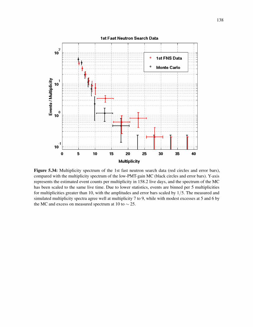
138

Figure 5.34: Multiplicity spectrum of the 1st fast neutron search data (red circles and error bars),compared with the multiplicity spectrum of the low-PMT-gain MC (black circles and error bars). Y-axisrepresents the estimated event counts per multiplicity in 158.2 live days, and the spectrum of the MChas been scaled to the same live time. Due to lower statistics, events are binned per 5 multiplicitiesfor multiplicities greater than 10, with the amplitudes and error bars scaled by 1/5. The measured andsimulated multiplicity spectra agree well at multiplicity 7 to 9, while with modest excesses at 5 and 6 bythe MC and excess on measured spectrum at 10 to ∼ 25.

139

Figure 5.35: Multiplicity spectrum of the 2nd fast neutron search data (red circles and error bars),compared with the multiplicity spectrum of the high-PMT-gain MC (black circles and error bars). Y-axisrepresents the estimated event counts per multiplicity in 169.2 live days, and the spectrum of the MC hasbeen scaled to the same live time. The spectrum is started with multiplicity 6, since the 2nd fast neutronsearch were run with multiplicity 6 in 70 µs trigger, instead of trigger at multiplicity 5. Due to lowerstatistics, events are binned per 5 multiplicities for multiplicities greater than 10, with the amplitudesand error bars scaled by 1/5. The measured and simulated multiplicity spectra agree generally well atmultiplicity 6 to 10, though there is modest excesses at 6 and 7 by the MC similar to the 1st fast neutronsearch data. There is excess on measured spectrum at 10 to ∼ 20.

140

Figure 5.36: Multiplicity spectrum of the 3rd fast neutron search data (red circles and error bars),compared with the multiplicity spectrum of the high-PMT-gain MC (black circles and error bars). Y-axisrepresents the estimated event counts per multiplicity in 302.8 live days, and the spectrum of the MC hasbeen scaled to stand for the same live time. Due to lower statistics, events are binned per 5 multiplicitiesfor multiplicities greater than 10, with the amplitudes and error bars scaled by 1/5. The measured andsimulated multiplicity spectra agree well at multiplicity 6 to 9, while excess on measured spectrumshows up at multiplicity 5 and multiplicity 10 to ∼ 20.

141

Then the amplitudes of low-gain spectrum AL(M) and high-gain spectrum AH(M) combine as

AC = sL ·AL + sH ·AH . (5.24)

Note when combining the uncertainties, the two spectra AL(M) and AH(M) are not independent.

They are both from the same simulation with the same live time, 138.2 days, although processed with

different PMT gain parameters and with independent random numbers for accepting photoelectrons.

The two spectra do convey some different information due to the different PMT gains. For example,

different fractions of real high-energy neutrons out of all accepted events and different gathering

powers result from the different PMT gains, and they could finally reflect on the difference of

the two multiplicity spectra. That is why the two spectra should be summed up with the proper

weights, instead of just using one of them. However, most of their uncertainties are from the same

MC. Therefore, the correct way of combining their uncertainty, in a conservative manner, is to sum

directly with weights,

σC = sL ·σL + sH ·σH . (5.25)

Figure 5.37 shows the multiplicity spectrum of high-energy neutrons with all the three fast

neutron search data sets combined compared against the spectrum simulated with the Geant4 based

comprehensive muon simulation. The spectrum represents the best estimate of the event numbers

of high-energy neutrons detected by the NMM as a function of multiplicity, in a total live time of

630.2 days. The combined spectrum cancels the discrepancies at multiplicities 5 to 7 appearing in

each data set in different ways, making the measurement and MC agree better at these multiplicities.

The measured event number at multiplicity 5 still slightly exceeds the prediction by the MC, but

within their error bars. The measured and simulated multiplicity spectra continue to agree up to

multiplicity 9. Then starting at multiplicity 10, the excess in the measured spectrum over MC

approximately with a factor of 3 is confirmed in the 630.2 days of live time combined results. The

142

excess exists with clear evidence up to multiplicity ∼ 20. For higher multiplicities, both measured

and MC spectra are limited by statistics, leaving the conclusion in this region ambiguous. However,

the higher expected event number of the measured spectrum than the MC spectrum in the 21-25 bin,

and the non-zero counts in 26-30 bin of the measurement, both hint of a possible continuation of

the excess of measured spectrum over MC.

The Neuntron Multiplicity Meter was proposed to measure the multiplicity as an approximation

or indication of the original energy of the high-energy (50MeV) neutron. However, according to

the analysis of the comprehensive muon simulation in Chapter 4, the accepted events include both

high-energy (50MeV) neutrons and low-energy multiple neutrons. It is impossible to extract a pure

multiplicity spectrum for just a high-energy neutrons. However, including the low-energy multiple

neutrons is expected to happen in both the real experimental run and the comprehensive muon

simulation. This makes a fair comparison between the the measured and simulated spectra.

As shown in Figure 4.23 and 4.24 in Chapter 4, the MC indicates that ∼ 2/3 of events of

multiplicity 10 or greater are detections of the neutrons with energies above 50 MeV. Therefore,

the excess in the measured spectrum at multiplicities 10 and greater may potentially suggest that

the energy spectrum of high-energy neutrons underground is harder than what is predicted by the

Geant4 MC. At this point, we are unable to prove this supposition with the data of the NMM.

In principle, it is possible that the underestimation of high-multiplicity events in the MC is from

underestimating the rate of low-energy multiple neutrons, instead of underestimating the rate of

high-energy neutrons. The former supposition could be linked to the neutron spallation cross section

in cavern rock, while the latter could be related to the cross sections for muons to interact with

cavern rock and generate high-energy neutrons. In other words, either the muon-induced neutrons

cause more spallations in cavern rock and thus result in more low-energy neutrons, or the cosmic-ray

muons themselves induce more high-energy neutrons, than the prediction of Geant4. It is also

possible that the excess is caused by both. In either case, it is all about muon-induced neutrons.

For the underground dark matter direct detection experiments, if the excess of neutron back-

143

Figure 5.37: Multiplicity spectrum of the combined fast neutron search (FNS) data, compared withthe MC multiplicity spectrum. The multiplicity spectrum in red circles and error bars is measured withall fast neutron search data of 630.2 days of live time. This result is obtained by combining all threespectra above measured with fast neutron search data sets, with appropiate weights based on their livetimes. The spectrum in black circles and error bars is resulted from the comprehensive muon simulationof 138.8 live days discussed in Chapter 4. Both spectra processed with the low-gain and high-gainparameters are combined with the weights based on the live times of low-gain and high-gain running infast neutron search. The uncertainties of low-gain and high-gain MC spectra are not independent, thusuncertainties of overall MC spectrum are combined as direct summation of the two with weights. Y-axisrepresents the estimated event counts per multiplicity in 630.2 live days, and the spectrum of MC hasbeen scaled to stand for the same live time. Due to lower statistics, events are binned per 5 multiplicitiesfor multiplicities greater than 10, with the amplitudes and error bars scaled by 1/5. The measuredand simulated multiplicity spectra agree well at multiplicity 5 to 9, with the previous discrepancies atmultiplicity 5 and 6 cleared after all data sets combined. The combined results confirm the excess onmeasured spectrum over MC approximately with a factor of 3, starting at multiplicity 10 and existing upto ∼ 20, or potentially to even higher multiplicities.

144

grounds is from low-energy (most likely below 10 MeV) multiple neutrons, the problem can be

easily solved by properly shielding with neutron moderating materials, such as water and high-

density polyethylene; if the excess is caused by more high-energy (above 50 MeV) cosmogenic

neutrons, then the neutron moderators are not able to stop them, also the inner gamma shielding

with high-Z materials, such as Pb and Cu, could help make the detector in danger of the multiple

secondary neutrons induced by the high-energy neutrons. In the latter case, the importance of

developing and building a neutron veto for the dark matter detector is raised.

To further study the source of the excess and narrow down the uncertainty of benchmarking,

it is worthwhile building and running experiments similar with the NMM at other underground

laboratories, with sufficient neutron moderator as shielding. The experiments can then exclude

the detection of low-energy neutrons, and test whether the excess of neutrons is due to a harder

spectrum of high-energy neutrons. These experiments would also result in more neutron flux data at

more underground sites, which is important to improve our understanding of cosmogenic neutron

backgrounds underground.

5.5 Measurement of the High-energy Neutron Flux at the Soudan

Underground Laboratory

The results of the LLR fits can also be used to measure the absolute flux of high-energy neutrons

with energies above 50 MeV detected by the NMM. This calculation needs the fraction of true

high-energy (> 50MeV) neutrons out of the overall accepted events and the gathering power found

in the comprehensive muon simulation in Chapter 4. The event rates in the low-gain run and the

high-gain runs should be treated separately with their own gathering powers.

Starting from the multiplicity spectrum of each fast neutron search run, the 1st run is during low

PMT gain, while the 2nd and 3rd runs are both during high PMT gain and their multiplicity spectra

may be combined. Let’s denote the multiplicity spectrum of the low-gain run with ALm±σL

m, and

145

the multiplicity spectrum of the high-gain run with AHm±σH

m , where the superscripts L and H for

low-gain and high-gain, respectively. The estimated total numbers of fast neutron events in low-gain

and high-gain runs are the sums of the series,

NL = ∑m

ALm ,

NH = ∑m

AHm ,

(5.26)

with the variances of the total event numbers of the two sets obtained by

σ2L = ∑

m(σL

m)2 ,

σ2H = ∑

m(σH

m )2 .

(5.27)

Using the multiplicity spetra of the three fast neutron search data sets resulted from the analysis

in Section 5.4, Eq. (5.26) and (5.27) give the estimated number of accepted events to be 150.4±11.3

in ∼ 158.2 live days of the 1st fast neutron search data (in low-gain), and 628.8±31.8 in ∼ 472.0

live days of the 2nd and 3rd fast neutron search data together (in high-gain). The relative uncertainties

of the two measurements are 7.5% and 5.1%, respectively.

According to Eq. (4.6), the definition of gathering power is the rate of accepted real high-energy

(> 50MeV) neutron events divided by the flux of high-energy neutrons above 50 MeV. But the

real high-energy (> 50MeV) neutron events are only a part of all accepted events. Here denote the

fraction of the real high-energy neutrons out of all accepted events as fL for low-gain run and fH for

high-gain run. They are estimated to be fL = (43±7)% and fH = (45±7)% with the MC truth

study in Chapter 4. Then the gathering power may further be written as

G =f ·N/TF

, (5.28)

where N stands for the total number of accepted events in the data set and T for the live time of the

146

data set. It is equivalent to

F ·T =f ·NG

, (5.29)

which can be understand as the total number of high-energy (> 50MeV) neutrons traversing in a

unit horizontal area during a run. Then given this quantities of the low-gain run and the high-gain

run, the flux of high-energy (> 50MeV) neutrons averaged over the two data sets is

F =FL ·TL +FH ·TH

TL +TH,

=fL ·NL/GL + fH ·NH/GH

Ttot.

(5.30)

And the uncertainty of the averaged flux can be calculated with

σF =1

Ttot

√(σ2fL

f 2L+

σ2NL

N2L+

σ2GL

G2L

)·( fLNL

GL

)2+(σ2

fH

f 2H

+σ2

NH

N2H

+σ2GH

G2H

)·( fHNH

GH

)2. (5.31)

The gathering power is estimated as (4.28±0.56)×103 cm2 for the low-gain run and

(5.02±0.61)×103 cm2 for the high-gain run with the MC in Chapter 4. The total live time of all

three fast neutron searches is 630.2 days (with actual precision up to 0.1 s used in the calculation).

By plugging the values of gathering powers and estimated event numbers in the two data sets

from the early part of this section in the Eq. (5.30) and (5.31), the flux of high-energy (> 50MeV)

neutrons at the Soudan Underground Laboratory is measured to be

(1.3±0.2)×10−9 cm−2s−1 .

The relative uncertainty is about 15%.

As mentioned earlier in this section, the relative uncertainties of the event counts or rate

147

measurements in low-gain and high-gain runs are only 7.5% and 5.1%, respectively. The dominant

uncertainty in the flux measurement is from the fractions of neutrons above 50 MeV out of all

accepted events and the gathering powers, which are limited by the statistics of the comprehensive

muon simulation. The relative uncertainties of these quantities decrease as ∼√

1/NMC, as the total

event number of MC NMC increases. It is estimated that if we had run the comprehensive muon

simulation of ∼ 400 days of live time, namely costing almost a factor of 3 of the CPU hours we had

for the MC, we could achieve a 10% measurement of the high-energy neutron flux, with the same

amount of data taken in the experiment.

D. Mei and A. Hime have given an MC estimation of the cosmogenic neutron flux for several sites

with different threshold energies with FLUKA [50]. Their simulated flux at the Soudan Underground

Laboratory is 4.73×10−9 cm−2s−1 above a threshold of 10 MeV, and 1.073×10−9 cm−2s−1 above

100 MeV. The measurement in this work is consistent with the range between the two values.

Chapter 6

Active Neutron Veto for SuperCDMS

Experiment at SNOLAB

An active neutron veto is vital for minimizing background level and achieving the desired sensitivity

for next-generation direct dark matter detection experiments. In this chapter, I present the design,

evaluation, and prototyping of the active neutron veto for SuperCDMS SNOLAB.

6.1 Passive Shieding for SuperCDMS SNOLAB

The next phase of the SuperCDMS experiment will be built and run at SNOLAB, with a depth

of 6,800 feet (6010 meter of water equivalent), reducing both cosmic-ray muons and cosmogenic

neutrons by more than two orders of magnitude.

The detectors will be surrounded by a layered shielding system, consisting of ultra-pure copper,

high-density polyethylene (HDPE) passive shielding layer, lead, and a combination of HDPE and

water tanks. Figure 6.1 shows the schematic layout with profile view and 3-dimensional view of the

cryostat and shielding layers. The goal of this shield is to reduce the flux of external gamma rays and

neutrons to a level that allows the detectors to achieve nearly background-free sensitivity. The copper

shielding is provided by the walls of the SNOBOX, which are multiple layers of ultra-pure copper,

148

149

Figure 6.1: Conceptual design of the SuperCDMS SNOLAB cryogenic and shielding system. On thetop is shown the 3-dimensional view. The dilution refrigerator on the left side of the diagram providesthe cooling for the thermal cans surrounding the detectors (center). A vacuum bulkhead and heat sinkingvessel (E-tank) is shown on the right. On the bottom is shown the profile view. A passive polyethyleneneutron shield, or an active neutron veto detector (gray), lies inside the lead shielding (light cyan), whichis surrounded by a massive polyethylene (bottom light cyan) and water shield (blue).

150

each 3/8”-1/2” thick. The iZIP detectors are located in the innermost can. The copper cans shield

the detectors from the particles emitted by radioactive contaminants in the environment. Copper is

the most radiopure material available with the mechanical properties that allow construction of such

large cans.

In the current baseline design, the second layer outward in the shielding system is a 40 cm

layer of HDPE. The thickness of this layer is more than necessary for passive shielding against the

external neutron flux, but it is to preserve space for a potential upgrade with an active neutron veto.

Surrounding the HDPE or active neutron veto is a ∼ 23cm thick layer of lead. The lead will be

from known sources that have low uranium and thorium contamination. The purpose of this layer is

to reduce the flux of external gamma rays.

Next to the lead shield is a thin metal sheet impervious to radon diffusion. The space within this

metal sheet will be constantly purged with dry nitrogen to prevent radon daughter deposition on the

surfaces that can result in radioactive contaminants near the detectors.

The outermost shielding is a 60 cm layer consisting of water tanks and a HDPE base. This layer

will reduce the neutron flux from the external environment. HDPE is commonly used for neutron

shielding, as it is efficient at neutron moderation and it provides mechnical support. But water

shielding is more economical for the top and sides of the layer.

Note there are two layers for neutron shielding. It is necessary to have both the outermost layer

and a layer adjacent the copper cans serving as neutron shielding. The outer water tanks and HDPE

is needed for reducing the neutron flux that can hit the lead layer. Then, as discussed in Chapter 2,

when high-energy neutrons hit the lead shielding, the lead itself may become an extra source of

neutrons, and it is pretty close to the detector. So within the lead layer, it is necessary to place a

HDPE shielding to reduce the additional neutron flux, or scintillator layer, as an active veto shield,

to tag neutron background events.

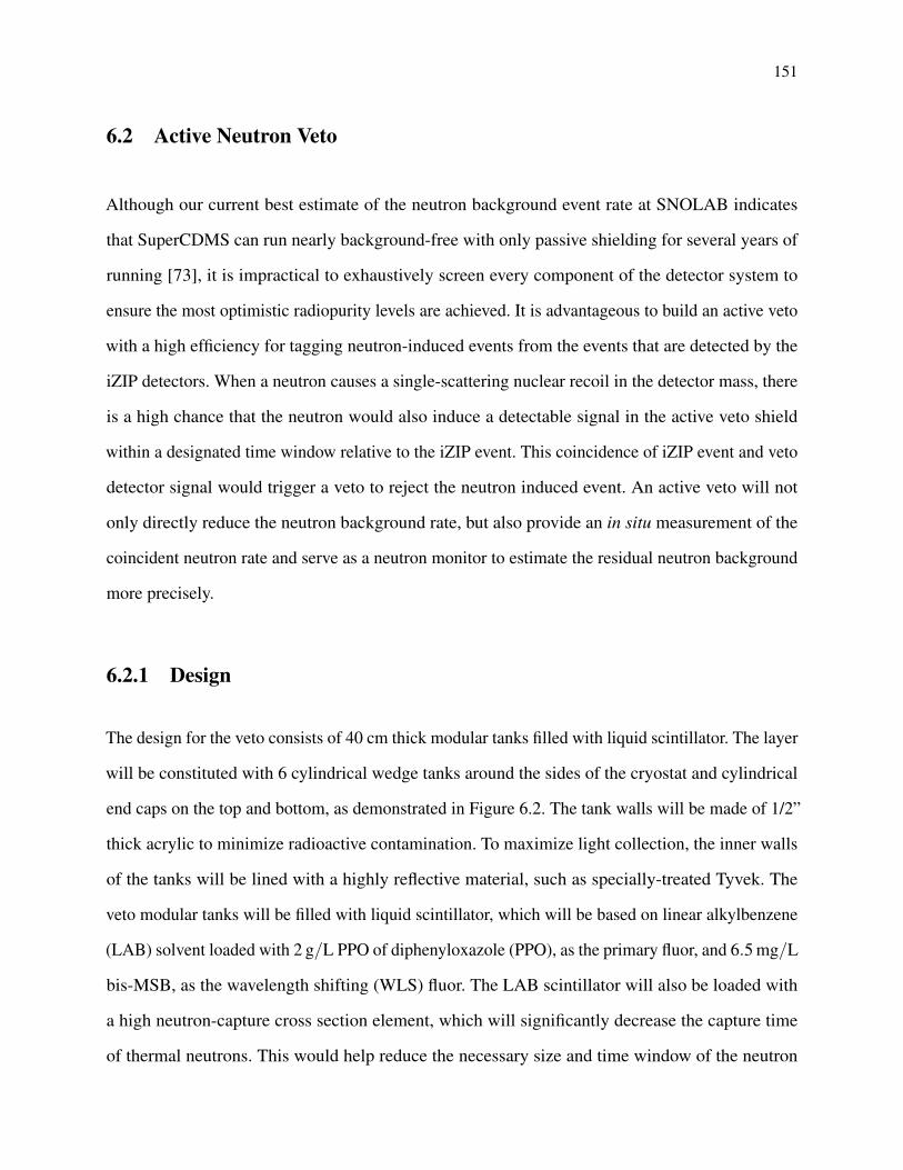
151

6.2 Active Neutron Veto

Although our current best estimate of the neutron background event rate at SNOLAB indicates

that SuperCDMS can run nearly background-free with only passive shielding for several years of

running [73], it is impractical to exhaustively screen every component of the detector system to

ensure the most optimistic radiopurity levels are achieved. It is advantageous to build an active veto

with a high efficiency for tagging neutron-induced events from the events that are detected by the

iZIP detectors. When a neutron causes a single-scattering nuclear recoil in the detector mass, there

is a high chance that the neutron would also induce a detectable signal in the active veto shield

within a designated time window relative to the iZIP event. This coincidence of iZIP event and veto

detector signal would trigger a veto to reject the neutron induced event. An active veto will not

only directly reduce the neutron background rate, but also provide an in situ measurement of the

coincident neutron rate and serve as a neutron monitor to estimate the residual neutron background

more precisely.

6.2.1 Design

The design for the veto consists of 40 cm thick modular tanks filled with liquid scintillator. The layer

will be constituted with 6 cylindrical wedge tanks around the sides of the cryostat and cylindrical

end caps on the top and bottom, as demonstrated in Figure 6.2. The tank walls will be made of 1/2”

thick acrylic to minimize radioactive contamination. To maximize light collection, the inner walls

of the tanks will be lined with a highly reflective material, such as specially-treated Tyvek. The

veto modular tanks will be filled with liquid scintillator, which will be based on linear alkylbenzene

(LAB) solvent loaded with 2 g/L PPO of diphenyloxazole (PPO), as the primary fluor, and 6.5 mg/L

bis-MSB, as the wavelength shifting (WLS) fluor. The LAB scintillator will also be loaded with

a high neutron-capture cross section element, which will significantly decrease the capture time

of thermal neutrons. This would help reduce the necessary size and time window of the neutron

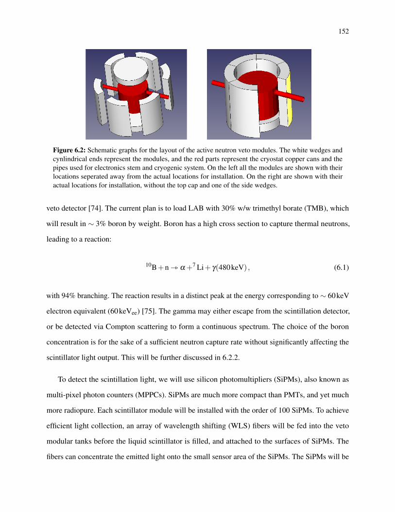
152

Figure 6.2: Schematic graphs for the layout of the active neutron veto modules. The white wedges andcynlindrical ends represent the modules, and the red parts represent the cryostat copper cans and thepipes used for electronics stem and cryogenic system. On the left all the modules are shown with theirlocations seperated away from the actual locations for installation. On the right are shown with theiractual locations for installation, without the top cap and one of the side wedges.

veto detector [74]. The current plan is to load LAB with 30% w/w trimethyl borate (TMB), which

will result in ∼ 3% boron by weight. Boron has a high cross section to capture thermal neutrons,

leading to a reaction:

10B+n _ α +7 Li+ γ(480keV) , (6.1)

with 94% branching. The reaction results in a distinct peak at the energy corresponding to ∼ 60keV

electron equivalent (60keVee) [75]. The gamma may either escape from the scintillation detector,

or be detected via Compton scattering to form a continuous spectrum. The choice of the boron

concentration is for the sake of a sufficient neutron capture rate without significantly affecting the

scintillator light output. This will be further discussed in 6.2.2.

To detect the scintillation light, we will use silicon photomultipliers (SiPMs), also known as

multi-pixel photon counters (MPPCs). SiPMs are much more compact than PMTs, and yet much

more radiopure. Each scintillator module will be installed with the order of 100 SiPMs. To achieve

efficient light collection, an array of wavelength shifting (WLS) fibers will be fed into the veto

modular tanks before the liquid scintillator is filled, and attached to the surfaces of SiPMs. The

fibers can concentrate the emitted light onto the small sensor area of the SiPMs. The SiPMs will be

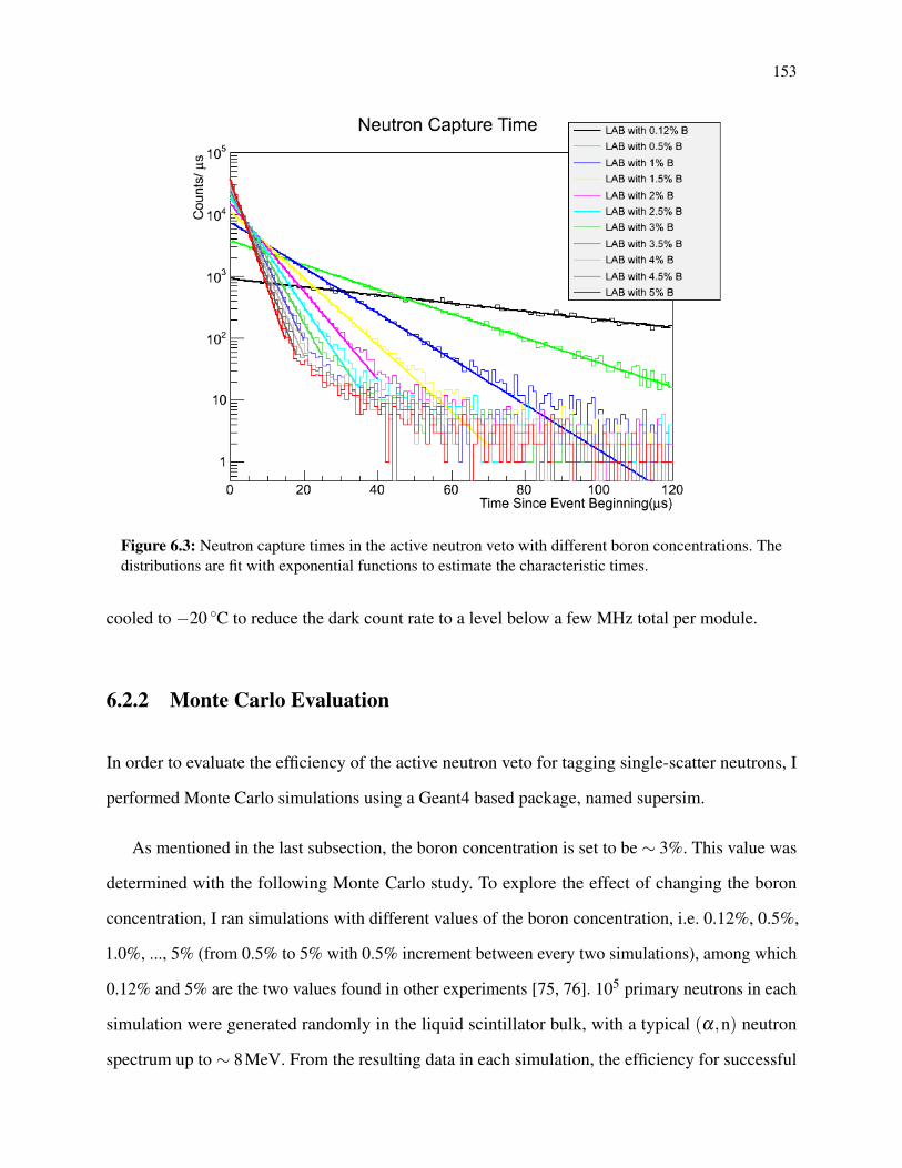
153

Figure 6.3: Neutron capture times in the active neutron veto with different boron concentrations. Thedistributions are fit with exponential functions to estimate the characteristic times.

cooled to −20 C to reduce the dark count rate to a level below a few MHz total per module.

6.2.2 Monte Carlo Evaluation

In order to evaluate the efficiency of the active neutron veto for tagging single-scatter neutrons, I

performed Monte Carlo simulations using a Geant4 based package, named supersim.

As mentioned in the last subsection, the boron concentration is set to be ∼ 3%. This value was

determined with the following Monte Carlo study. To explore the effect of changing the boron

concentration, I ran simulations with different values of the boron concentration, i.e. 0.12%, 0.5%,

1.0%, ..., 5% (from 0.5% to 5% with 0.5% increment between every two simulations), among which

0.12% and 5% are the two values found in other experiments [75, 76]. 105 primary neutrons in each

simulation were generated randomly in the liquid scintillator bulk, with a typical (α,n) neutron

spectrum up to ∼ 8MeV. From the resulting data in each simulation, the efficiency for successful

154

Figure 6.4: Estimated neutron tagging efficiency, plotted together with capture time, both as functionsof boron concentration. The tagging efficiency with infinite time is in the blue box and solid line, and thetagging efficiency with a 100 µs veto time window is in the red box and solid line, with both labeled bythe left-hand Y-axis. The neutron capture time is in the green empty box and dashed line, labeled bythe right-hand Y-axis. The tagging efficiency (capture time) increases (decreases) dramatically as boronconcentration increases at low values, while the changes of both slow down with respect to the change ofboron concentration at higher values.

155

tagging of the single-scatter neutron events in iZIPs was calculated, and the times of captures since

the event beginning were collected to histograms. Figure 6.3 shows the capture time distribution for

different boron concentrations. Fit with exponential functions is performed for each distribution to

obtain the characteristic time of capture (or simply called capture time). In Figure 6.4, the tagging

efficiencies (called Fraction of Captured Neutrons in the Y-axis label) are plotted together with

capture times, with the left-hand side of the Y-axis representing the tagging efficiency and the

right-hand side of the Y-axis representing capture time. As boron concentration increases from

0.12% to 1.5%, the tagging efficiency dramatically increases above 0.9, and the capture time goes

below 10 µs; as boron concentration continues to increase, both the increase of tagging efficiency

and dropping of capture time slow down. The plot clearly indicates that any value beyond 3% would

not significantly improve tagging efficiency. Given that a 3% boron concentration already requires a

load of 30% TMB, too much doping can dramatically hurt the light transparency and result in bad

light collection. Therefore, we believe that a 3% boron concentration is a reasonable choice. In the

figure, a comparison is also made between the tagging efficiencies with infinite time and with a time

window of 100 µs. It is shown that the efficiency with 100 µs veto time would not be significantly

lower than that with infinite time. In realistic experimental running, the order of 100 µs for the event

time is a reasonable setting.

Another Monte Carlo simulation study was performed to test the veto time window and veto

threshold. 105 primary neutrons were initiated from the outermost layer of the copper cans, the

“outer vessel can” (OVC), and the data were analyzed with different settings of veto time windows.

The results, shown in Figure 6.5, are veto efficiency as a funcion of veto threshold in keVee (keV

electron-equivalent energy) for different values of the veto time window. With a 50 keVee threshold

and 100 µs veto time window, the veto efficiency is estimated to be (92.2±0.9)% for single-scatter

neutron-induced nuclear recoil events in iZIP detectors.

From the other simulations of radioactive contaminations in the shield and veto materials, the

rate of background events in the veto detector above 50 keVee threshold is estimated to be less than

156

Figure 6.5: Veto efficiency for tagging single-scatter neutron-induced iZIP events as a function ofthreshold energy in keVee, for veto time window 10 µs (black), 30 µs (red), 100 µs (green), and 300 µs(blue). A higher threshold energy or a shorter veto time window results in a lower veto efficiency. Theparamters chosen in the current design are a threshold of 50 keVee and 100 µs, which are demonstratedto be able to achieve a veto efficiency of 92-93%.

157

200 Hz, resulting in < 2% veto-induced live-time loss with a 100 µs window. We therefore believe

that this design of active neutron veto will meet the goal of 90% veto efficiency without significant

negative impact on dark matter search efficiency. In addition, the rate of the neutrons tagged by the

active neutron veto can be used to estimate the rate of the residual neutron backgrounds, helping the

neutron veto serve as a more precise neutron monitor.

6.3 Prototyping of the Neutron Veto

The design requirement of the active neutron veto, i.e. using 100 µs window, triggering events

at a 50 keVee threshold, and tagging single-scatter neutron events with 90% efficiency, will be

achieved by focusing on two aspects: maximization of the amount of energy deposited in the veto by

neutron-induced events, and ensuring sufficient light is produced, collected, and detected in the veto

system. The simulation evaluation that was done was based on a simplified geometry, and tallying

with energy deposition without optical simulations. All the information on a more detailed geometry

and the parameters associated with optical components needed to be explored and collected to

further develop the veto. It was wise and necessary to start with a prototype detector.

6.3.1 The Quarter-Scale Prototype

We designed and constructed a neutron-detector prototype with approximately one quarter the size

of a single full size module. A box shape was used instead of the curved wedge module geometry to

simplify construction and assembly. The prototype dimensions were 23×12×3.75 inches, assembled

out of 0.5 inch thick clear acrylic. To maximize the light collection efficiency, the inner surface of

the acrylic vessel were lined with Lumirror reflector, as can be seen in Figure 6.6 left. The prototype

was strung with 16 1.5 mm diameter Kuraray Y-11 WLS fibers through holes drilled through the

acrylic and sealed with 5-minute epoxy. Each fiber was 28 inches long and was bundled into groups

of four at each end. The fiber readout was accomplished using 8 Hamamatsu S12572-100C 3 mm

158

Figure 6.6: The photographs of the quarter-scale neutron-veto prototype. On the left in shown one endof the liquid scintillator prototype before it was sealed. The SiPMs are mounted to the Al cooling plateand are coupled to the fibers that are fed through the holes on the ends of the acrylic vessel into the liquidscintillator. On the right is shown the dark box after the SiPMs were installed but before the acrylicvessel was inserted. The measurements were conducted in the dark box that was held under nitrogenpurge.

SiPMs, one for each end of the 4-fiber bundle. Custom mounts were constructed to mount the fiber

ends over the face of the SiPM. The SiPMs were mounted on a cooling plate in order to reduce the

dark rate.

The entire assembly was housed in a dark box, as shown in Figure 6.6 right, under a fume

hood for safety. The atmosphere in the dark box was held under a nitrogen purge to reduce the

flammability hazard of the TMB and to prevent condensation from forming on the SiPMs.

6.3.2 Monte Carlo Model

The Geant4 Monte Carlo package supersim works in tallying energy deposition, but does not

perform an optical simulation. The MC performed to evaluate the overall design of the neutron veto

hence does not provide the information on optimizing the light collection. An integrated method of

simulation including both the process of particle interaction and transportation, and the process of

optical simulation, would be rather time consuming, and inefficient for understanding the optical

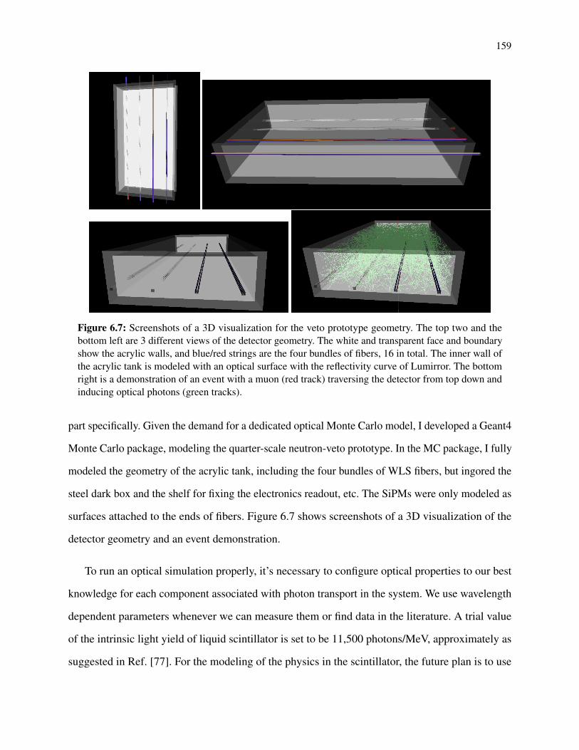
159

Figure 6.7: Screenshots of a 3D visualization for the veto prototype geometry. The top two and thebottom left are 3 different views of the detector geometry. The white and transparent face and boundaryshow the acrylic walls, and blue/red strings are the four bundles of fibers, 16 in total. The inner wall ofthe acrylic tank is modeled with an optical surface with the reflectivity curve of Lumirror. The bottomright is a demonstration of an event with a muon (red track) traversing the detector from top down andinducing optical photons (green tracks).

part specifically. Given the demand for a dedicated optical Monte Carlo model, I developed a Geant4

Monte Carlo package, modeling the quarter-scale neutron-veto prototype. In the MC package, I fully

modeled the geometry of the acrylic tank, including the four bundles of WLS fibers, but ingored the

steel dark box and the shelf for fixing the electronics readout, etc. The SiPMs were only modeled as

surfaces attached to the ends of fibers. Figure 6.7 shows screenshots of a 3D visualization of the

detector geometry and an event demonstration.

To run an optical simulation properly, it’s necessary to configure optical properties to our best

knowledge for each component associated with photon transport in the system. We use wavelength

dependent parameters whenever we can measure them or find data in the literature. A trial value

of the intrinsic light yield of liquid scintillator is set to be 11,500 photons/MeV, approximately as

suggested in Ref. [77]. For the modeling of the physics in the scintillator, the future plan is to use

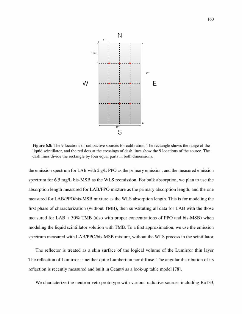
160

Figure 6.8: The 9 locations of radioactive sources for calibration. The rectangle shows the range of theliquid scintillator, and the red dots at the crossings of dash lines show the 9 locations of the source. Thedash lines divide the rectangle by four equal parts in both dimensions.

the emission spectrum for LAB with 2 g/L PPO as the primary emission, and the measured emission

spectrum for 6.5 mg/L bis-MSB as the WLS reemission. For bulk absorption, we plan to use the

absorption length measured for LAB/PPO mixture as the primary absorption length, and the one

measured for LAB/PPO/bis-MSB mixture as the WLS absorption length. This is for modeling the

first phase of characterization (without TMB), then substituting all data for LAB with the those

measured for LAB + 30% TMB (also with proper concentrations of PPO and bis-MSB) when

modeling the liquid scintillator solution with TMB. To a first approximation, we use the emission

spectrum measured with LAB/PPO/bis-MSB mixture, without the WLS process in the scintillator.

The reflector is treated as a skin surface of the logical volume of the Lumirror thin layer.

The reflection of Lumirror is neither quite Lambertian nor diffuse. The angular distribution of its

reflection is recently measured and built in Geant4 as a look-up table model [78].

We characterize the neutron veto prototype with various radiative sources including Ba133,

161

Cs137, Co60, Cf125 etc., and with cosmic ray mode. In radiative source runs, the sources are set in 9

fixed locations on the top of the steel dark box, as shown in Figure 6.8. The idea for determining the

unknown optical paramters is to run the same radioactive sources with the same array of locations in

the simulations. For each location use the PE spectra obtained in the 8 channels to fit the measured

PE distributions. While tuning the parameters and running the simulation again and again, the

parameters would be trained to best fit the simulated PE spectra with the measured ones. In this

section, I only present a primary simulation that demonstrates the MC model for the prototype.

In this demonstrative MC study, 137Cs are set collimated at East, Center, and West source

locations. There are 105 primary gammas simulated in each case, conforming to the 137Cs spectrum.

The deposited energy spectrum and photoelectron spectrum are shown in Figure 6.9, for the three

source locations. In order to measure light yield and energy resolution, we fit the PE spectrum with

the deposited energy distribution convoluted with a gaussian function with the standard deviation

σ =√

A ·PE , (6.2)

where A is a dimensionless constant and PE = (LightYield) ·Edep. In the fit info box of the plots,

p0 is a normalization factor that scales the amplitude, p1 is the Light Yield in PE/MeV, and p2 is

the constant A. According to the fit results, the light yield is about 0.36 PE/keV, so that a 50 keV

threshold is equivalent to ∼ 18 PE. The energy resolution near the threshold is about 24-25%.

Figure 6.10 shows the fraction of individual channel PE over the total PE (in the left column),

and the PE spectra in individual channels, for the different source locations. As can be seen, the

channels that are closer to the source get harder spectra. The distribution of the individual channel

response is sensitive to the source location, and can be used to tune the unknown optical parameters

in the model with a large batch of simulations.

Since the active neutron veto was not funded in the baseline development of SuperCDMS

SNOLAB, the prototyping work has stopped. If the collaboration continues the neutron-veto

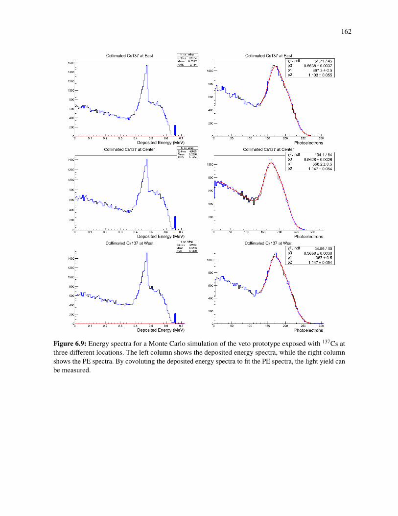
162

Figure 6.9: Energy spectra for a Monte Carlo simulation of the veto prototype exposed with 137Cs atthree different locations. The left column shows the deposited energy spectra, while the right columnshows the PE spectra. By covoluting the deposited energy spectra to fit the PE spectra, the light yield canbe measured.

163

Figure 6.10: The left column shows the fraction of PE response of individual channels over the totalPE. The right column shows channel number vs the PE fraction, with the color representing event rate.The chanels closer to the source location get harder spectra. The sensitivity of the individual channelresponse to the source locations can be used to tune the unknown optical parameters with a large batchof simulations.

164

prototyping, the method discussed in this section will be resumed to train the model parameters for

the optical simulation. In addition, the simulation study in this section demonstrated that light yield

and energy resolution can be meausured with this MC model by convoluting the deposited energy

spectrum to fit the PE spectrum.

6.3.3 Demonstration Runs

Data were taken for a variety of radioactive sources. The sources were used to calibrate the SiPM

response and the light yield of the prototype. Figure 6.11 shows the measured 137Cs spectrum

compared to a Geant4 spectrum smeared using parameters derived from 137Cs data and SiPM

response. From this comparison, the light yield is tuned to be 520 PE/MeV to match the shoulder

and falling feature between the measured spectrum and Geant4 spectrum.

The energy spectrum is also measured without any radioactive source present. As shown in

Figure 6.12, the peak around 16 MeV corresponds to cosmic muons passing through the detector.

Figure 6.11: The measured spectrum of 137Cs compared to a Geant4 137Cs spectrum smeared usingparameters derived from 137Cs and SiPM response. Figure by Ben Loer, FNAL.

165

Figure 6.12: The measured energy spectrum for data collected without any radioactive source present.The peak around 16 MeV corresponds to cosmic muons passing through the detector, depositing energyas least ionizing particles. The Geant4 energy spectrum has been convoluted with a smearing functionderived from 137Cs data. The energy scale/light yield has been obtained by aligning the data and MonteCarlo peaks by eye. Figure by Ben Loer, FNAL.

Muons are least ionizing particles, and the energy deposition is determined by the path length in

the detector scintillator, and estimated to be ∼ 16MeV for the thinkness of the liquid scintillator in

the prototype. By aligning the peaks of the data and the Monte Carlo, the light yield is tuned to be

235 PE/MeV in the muon run. The true light yield is likely between 0.2-0.5 PE/keV.

When taking data with 252Cf, we were unable to observe the expected 60keVee peak as the

signature of boron neutron captures. The reason is not completely understood, but the large gamma

background emitted by the same 252Cf source may be overwhelming the capture signal. It may also

be that the energy resolution was too poor to distinguish the neutron capture peak.

At present, since the active neutron veto is not under the baseline plan of SuperCDMS SNOLAB,

the work on prototyping has fallen in low priority. If in the future the the collaboration is proved to

upgrade the passvie shield with the active neutron veto, there may be a lot of follow-up on analyzing,

understanding the demonstrative runs, and improving the design of the prototype and the full-scale

166

modules. We may use collimated neutron source to measure the neutron response, or try to shield

against gamma rays. We would also need to perform more simulations to reveal potential issues in

the system. Finally, with a better undertanding of the prototype detector, there may more hints to

improve the design for more efficient light collection and better energy resolution.

167

References

[1] Scott Dodelson. Modern cosmology. San Diego, CA: Academic Press, 2003. U R L : https:

//cds.cern.ch/record/1282338 (cit. on pp. 1, 9).

[2] Sean M. Carroll. Spacetime and geometry: An introduction to general relativity. Pearson In-

ternational, 2004. U R L : http://www.slac.stanford.edu/spires/find/books/www?

cl=QC6:C37:2004 (cit. on p. 1).

[3] Planck Collaboration. “Planck 2015 results - I. Overview of products and scientific results”.

In: A&A 594 (2016), A1. D O I : 10.1051/0004-6361/201527101. U R L : http://dx.doi.

org/10.1051/0004-6361/201527101 (cit. on p. 3).

[4] S. Burles, K. M. Nollett, and Michael S. Turner. “Deuterium and big bang nucleosynthesis”.

In: Nucl. Phys. A663 (2000), pp. 861c–864c. D O I : 10.1016/S0375-9474(99)00732-0.

arXiv: astro-ph/9903300 [astro-ph] (cit. on pp. 4, 5).

[5] F. Zwicky. “The redshift of extragalactic nebulae”. In: Helv. Phys. Acta 6 (1933). [Gen. Rel.

Grav.41,207(2009)], pp. 110–127. D O I : 10.1007/s10714-008-0707-4 (cit. on p. 6).

[6] Vera C. Rubin and W. Kent Ford Jr. “Rotation of the Andromeda Nebula from a Spectroscopic

Survey of Emission Regions”. In: Astrophys. J. 159 (1970), pp. 379–403. D O I : 10.1086/

150317 (cit. on pp. 6, 7).

[7] Edvige Corbelli and Paolo Salucci. “The Extended Rotation Curve and the Dark Matter

Halo of M33”. In: Mon. Not. Roy. Astron. Soc. 311 (2000), pp. 441–447. D O I : 10.1046/j.

1365-8711.2000.03075.x. arXiv: astro-ph/9909252 [astro-ph] (cit. on pp. 6, 7).

https://cds.cern.ch/record/1282338

https://cds.cern.ch/record/1282338

http://www.slac.stanford.edu/spires/find/books/www?cl=QC6:C37:2004

http://www.slac.stanford.edu/spires/find/books/www?cl=QC6:C37:2004

http://dx.doi.org/10.1051/0004-6361/201527101

http://dx.doi.org/10.1051/0004-6361/201527101

http://dx.doi.org/10.1051/0004-6361/201527101

http://dx.doi.org/10.1016/S0375-9474(99)00732-0

http://arxiv.org/abs/astro-ph/9903300

http://dx.doi.org/10.1007/s10714-008-0707-4

http://dx.doi.org/10.1086/150317

http://dx.doi.org/10.1086/150317

http://dx.doi.org/10.1046/j.1365-8711.2000.03075.x

http://dx.doi.org/10.1046/j.1365-8711.2000.03075.x


168

[8] Isabelle Paris et al. “The Sloan Digital Sky Survey quasar catalog: ninth data release”.

In: Astron. Astrophys. 548 (2012), A66. D O I : 10.1051/0004-6361/201220142. arXiv:

1210.5166 [astro-ph.CO] (cit. on p. 6).

[9] Will Saunders et al. “The PSCz catalogue”. In: Mon. Not. Roy. Astron. Soc. 317 (2000), p. 55.

D O I : 10.1046/j.1365-8711.2000.03528.x. arXiv: astro-ph/0001117 [astro-ph]

(cit. on p. 9).

[10] Andrew J. S. Hamilton and Max Tegmark. “The Real space power spectrum of the PSCz

survey from 0.01 to 300 h Mpc**-1”. In: Mon. Not. Roy. Astron. Soc. 330 (2002), p. 506.

D O I : 10.1046/j.1365-8711.2002.05033.x. arXiv: astro-ph/0008392 [astro-ph]

(cit. on p. 9).

[11] Adam G. Riess et al. “Observational evidence from supernovae for an accelerating universe

and a cosmological constant”. In: Astron. J. 116 (1998), pp. 1009–1038. D O I : 10.1086/

300499. arXiv: astro-ph/9805201 [astro-ph] (cit. on p. 6).

[12] P. Sikivie. “Experimental Tests of the ”Invisible” Axion”. In: Phys. Rev. Lett. 51 (16 Oct.

1983), pp. 1415–1417. D O I : 10.1103/PhysRevLett.51.1415. U R L : http://link.aps.

org/doi/10.1103/PhysRevLett.51.1415 (cit. on p. 10).

[13] Hsin-Chia Cheng, Jonathan L. Feng, and Konstantin T. Matchev. “Kaluza-Klein Dark Matter”.

In: Phys. Rev. Lett. 89 (21 Oct. 2002), p. 211301. D O I : 10.1103/PhysRevLett.89.211301.

U R L : http://link.aps.org/doi/10.1103/PhysRevLett.89.211301 (cit. on p. 10).

[14] Fumihiro Takayama and Masahiro Yamaguchi. “Gravitino dark matter without R-parity”. In:

Phys. Lett. B485 (2000), pp. 388–392. D O I : 10.1016/S0370-2693(00)00726-7. arXiv:

hep-ph/0005214 [hep-ph] (cit. on p. 10).

[15] Benjamin W. Lee and Steven Weinberg. “Cosmological Lower Bound on Heavy Neutrino

Masses”. In: Phys. Rev. Lett. 39 (1977), pp. 165–168. D O I : 10.1103/PhysRevLett.39.

165 (cit. on p. 10).

[16] H.E. Haber and G.L. Kane. “The search for supersymmetry: Probing physics beyond the stan-

dard model”. In: Physics Reports 117.2 (1985), pp. 75–263. D O I : http://dx.doi.org/10.

http://dx.doi.org/10.1051/0004-6361/201220142

http://arxiv.org/abs/1210.5166

http://dx.doi.org/10.1046/j.1365-8711.2000.03528.x


http://dx.doi.org/10.1046/j.1365-8711.2002.05033.x


http://dx.doi.org/10.1086/300499

http://dx.doi.org/10.1086/300499


http://dx.doi.org/10.1103/PhysRevLett.51.1415

http://link.aps.org/doi/10.1103/PhysRevLett.51.1415




http://dx.doi.org/10.1016/S0370-2693(00)00726-7

http://arxiv.org/abs/hep-ph/0005214



http://dx.doi.org/http://dx.doi.org/10.1016/0370-1573(85)90051-1


169

1016/0370-1573(85)90051-1. U R L : http://www.sciencedirect.com/science/article/

pii/0370157385900511 (cit. on p. 10).

[17] Edward W. Kolb and Michael S. Turner. “The Early Universe”. In: Front. Phys. 69 (1990),

pp. 1–547 (cit. on pp. 10, 11).

[18] Gerard Jungman, Marc Kamionkowski, and Kim Griest. “Supersymmetric dark matter”.

In: Phys. Rept. 267 (1996), pp. 195–373. D O I : 10.1016/0370-1573(95)00058-5. arXiv:

hep-ph/9506380 [hep-ph] (cit. on p. 11).

[19] Andrew Hime. “The MiniCLEAN Dark Matter Experiment”. In: Particles and fields. Pro-

ceedings, Meeting of the Division of the American Physical Society, DPF 2011, Providence,

USA, August 9-13, 2011. 2011. arXiv: 1110.1005 [physics.ins-det]. U R L : https:

//inspirehep.net/record/930736/files/arXiv:1110.1005.pdf (cit. on pp. 11, 16).

[20] K. Rielage et al. “Update on the MiniCLEAN Dark Matter Experiment”. In: Phys. Proce-

dia 61 (2015), pp. 144–152. D O I : 10.1016/j.phpro.2014.12.024. arXiv: 1403.4842

[physics.ins-det] (cit. on pp. 11, 16).

[21] P. -A. Amaudruz et al. “DEAP-3600 Dark Matter Search”. In: Proceedings, 37th Interna-

tional Conference on High Energy Physics (ICHEP 2014): Valencia, Spain, July 2-9, 2014.

Vol. 273-275. 2016, pp. 340–346. D O I : 10.1016/j.nuclphysbps.2015.09.048. arXiv:

1410.7673 [physics.ins-det]. U R L : https://inspirehep.net/record/1324765/

files/arXiv:1410.7673.pdf (cit. on pp. 11, 16).

[22] D. S. Akerib et al. “The Large Underground Xenon (LUX) Experiment”. In: Nucl. Instrum.

Meth. A704 (2013), pp. 111–126. D O I : 10.1016/j.nima.2012.11.135. arXiv: 1211.

3788 [physics.ins-det] (cit. on pp. 11, 16).

[23] E. Aprile et al. “The XENON100 dark matter experiment”. In: Astroparticle Physics 35.9

(2012), pp. 573–590. D O I : http://dx.doi.org/10.1016/j.astropartphys.2012.01.

003. U R L : http://www.sciencedirect.com/science/article/pii/S0927650512000059

(cit. on pp. 11, 16).

[24] P. Agnes et al. “Results from the first use of low radioactivity argon in a dark matter search”.



http://www.sciencedirect.com/science/article/pii/0370157385900511


http://dx.doi.org/10.1016/0370-1573(95)00058-5



https://inspirehep.net/record/930736/files/arXiv:1110.1005.pdf


http://dx.doi.org/10.1016/j.phpro.2014.12.024



http://dx.doi.org/10.1016/j.nuclphysbps.2015.09.048




http://dx.doi.org/10.1016/j.nima.2012.11.135



http://dx.doi.org/http://dx.doi.org/10.1016/j.astropartphys.2012.01.003

http://dx.doi.org/http://dx.doi.org/10.1016/j.astropartphys.2012.01.003

http://www.sciencedirect.com/science/article/pii/S0927650512000059

170

In: Phys. Rev. D93.8 (2016), p. 081101. D O I : 10.1103/PhysRevD.93.081101. arXiv:

1510.00702 [astro-ph.CO] (cit. on pp. 11, 16).

[25] R. Agnese et al. “Demonstration of Surface Electron Rejection with Interleaved Germanium

Detectors for Dark Matter Searches”. In: Appl. Phys. Lett. 103 (2013), p. 164105. D O I :

10.1063/1.4826093. arXiv: 1305.2405 [physics.ins-det] (cit. on pp. 11, 16, 27).

[26] E. Armengaud et al. “First results of the EDELWEISS-II WIMP search using Ge cryogenic

detectors with interleaved electrodes”. In: Phys. Lett. B687 (2010), pp. 294–298. D O I :

10.1016/j.physletb.2010.03.057. arXiv: 0912.0805 [astro-ph.CO] (cit. on pp. 11,

16).

[27] C. E. Aalseth et al. “Results from a Search for Light-Mass Dark Matter with a P-type

Point Contact Germanium Detector”. In: Phys. Rev. Lett. 106 (2011), p. 131301. D O I :

10.1103/PhysRevLett.106.131301. arXiv: 1002.4703 [astro-ph.CO] (cit. on pp. 11,

16).

[28] Marco Battaglia, Ian Hinchliffe, and Daniel Tovey. “Cold dark matter and the LHC”. In: J.

Phys. G30 (2004), R217–R244. D O I : 10.1088/0954-3899/30/10/R01. arXiv: hep-ph/

0406147 [hep-ph] (cit. on p. 12).

[29] Gianfranco Bertone, Dan Hooper, and Joseph Silk. “Particle dark matter: Evidence, candi-

dates and constraints”. In: Phys. Rept. 405 (2005), pp. 279–390. D O I : 10.1016/j.physrep.

2004.08.031. arXiv: hep-ph/0404175 [hep-ph] (cit. on p. 12).

[30] Mark W. Goodman and Edward Witten. “Detectability of Certain Dark Matter Candidates”.

In: Phys. Rev. D31 (1985), p. 3059. D O I : 10.1103/PhysRevD.31.3059 (cit. on p. 12).

[31] Joel R. Primack, David Seckel, and Bernard Sadoulet. “Detection of Cosmic Dark Matter”.

In: Ann. Rev. Nucl. Part. Sci. 38 (1988), pp. 751–807. D O I : 10.1146/annurev.ns.38.

120188.003535 (cit. on p. 12).

[32] R. W. Schnee. “Introduction to dark matter experiments”. In: In Physics of the Large and

Small: Proceedings of the 2009 Theoretical Advanced Study Institute in Elementary Particle

Physics, 629-681 (World Scientific, Singapore) Ed. Csaba Csaki and Scott Dodelson (2010).

http://dx.doi.org/10.1103/PhysRevD.93.081101


http://dx.doi.org/10.1063/1.4826093


http://dx.doi.org/10.1016/j.physletb.2010.03.057




http://dx.doi.org/10.1088/0954-3899/30/10/R01



http://dx.doi.org/10.1016/j.physrep.2004.08.031

http://dx.doi.org/10.1016/j.physrep.2004.08.031



http://dx.doi.org/10.1146/annurev.ns.38.120188.003535

http://dx.doi.org/10.1146/annurev.ns.38.120188.003535

171

2011. arXiv: 1101.5205 [astro-ph.CO]. U R L : https://inspirehep.net/record/

885795/files/arXiv:1101.5205.pdf (cit. on p. 12).

[33] J. D. Lewin and P. F. Smith. “Review of mathematics, numerical factors, and corrections

for dark matter experiments based on elastic nuclear recoil”. In: Astropart. Phys. 6 (1996),

pp. 87–112. D O I : 10.1016/S0927-6505(96)00047-3 (cit. on p. 15).

[34] J. Filippini. “A Search for WIMP Dark Matter Using the First Five-Tower Run of the

Cryogenic Dark Matter Search”. PhD thesis. University of California, Berkeley, 2008 (cit. on

p. 15).

[35] David G. Cerdeno and Anne M. Green. “Direct detection of WIMPs”. In: Particle Dark

Matter: Observations, Models and Searches (2010). arXiv: 1002.1912 [astro-ph.CO]

(cit. on p. 15).

[36] D. S. Akerib et al. “Improved Limits on Scattering of Weakly Interacting Massive Particles

from Reanalysis of 2013 LUX Data”. In: Phys. Rev. Lett. 116.16 (2016), p. 161301. D O I :

10.1103/PhysRevLett.116.161301. arXiv: 1512.03506 [astro-ph.CO] (cit. on p. 16).

[37] D. S. Akerib et al. “Results on the Spin-Dependent Scattering of Weakly Interacting Massive

Particles on Nucleons from the Run 3 Data of the LUX Experiment”. In: Phys. Rev. Lett.

116.16 (2016), p. 161302. D O I : 10.1103/PhysRevLett.116.161302. arXiv: 1602.03489

[hep-ex] (cit. on p. 16).

[38] Joseph A. Formaggio and C.J. Martoff. “BACKGROUNDS TO SENSITIVE EXPERI-

MENTS UNDERGROUND”. In: Annual Review of Nuclear and Particle Science 54.1 (2004),

pp. 361–412. D O I : 10.1146/annurev.nucl.54.070103.181248. eprint: http://dx.

doi.org/10.1146/annurev.nucl.54.070103.181248. U R L : http://dx.doi.org/10.

1146/annurev.nucl.54.070103.181248 (cit. on p. 18).

[39] Eric B. Norman, Timothy E. Chupp, Kevin T. Lesko, Peter Schwalbach, and Patrick J. Grant.

“26g,mAl production cross sections from the 23Na(α , n)26Al reaction”. In: Nuclear Physics A

390.3 (1982), pp. 561–572. D O I : http://dx.doi.org/10.1016/0375-9474(82)90283-4.

U R L : http://www.sciencedirect.com/science/article/pii/0375947482902834 (cit.




http://dx.doi.org/10.1016/S0927-6505(96)00047-3







http://dx.doi.org/10.1146/annurev.nucl.54.070103.181248







172

on p. 19).

[40] Eric B. Norman, Timothy E. Chupp, Kevin T. Lesko, Patrick J. Grant, and Gene L. Woodruff.

“22Na production cross sections from the 19F(α,n) reaction”. In: Phys. Rev. C 30 (4 Oct.

1984), pp. 1339–1340. D O I : 10.1103/PhysRevC.30.1339. U R L : http://link.aps.

org/doi/10.1103/PhysRevC.30.1339 (cit. on p. 19).

[41] R. Heaton et al. “” In: Nucl. Geophys. V4 (1990), p. 499 (cit. on pp. 19, 20).

[42] R. K. Heaton, H. W. Lee, B. C. Robertson, E. B. Norman, K. T. Lesko, and B. Sur. “α-Particle

induced high-energy γ-ray yields from light elements”. In: Nuclear Instruments and Methods

in Physics Research A 364 (Feb. 1995), pp. 317–327. D O I : 10.1016/0168-9002(95)

00220-0 (cit. on p. 19).

[43] D. -M. Mei, C. Zhang, and A. Hime. “Evaluation of (alpha,n) Induced Neutrons as a Back-

ground for Dark Matter Experiments”. In: Nucl. Instrum. Meth. A606 (2009), pp. 651–660.

D O I : 10.1016/j.nima.2009.04.032. arXiv: 0812.4307 [nucl-ex] (cit. on pp. 20, 21).

[44] J. Koning, S. Hilaire, and M.C. Duijvestijn. “TALYS: comprehensive nuclear reaction mod-

eling”. In: Proceedings of the International Conference on Nuclear Data for Science and

Technology-ND2004 769 (2004), p. 1154 (cit. on p. 20).

[45] Cross Section Evaluation Working Group. ENDF/B-VI.8 Evaluated Nuclear Data Library.

U R L : http://www.nndc.bnl.gov/endf/b6.8/ (cit. on pp. 20, 40).

[46] A.J. Koning and D. Rochman. “Modern Nuclear Data Evaluation with the TALYS Code Sys-

tem”. In: Nuclear Data Sheets 113.12 (2012), pp. 2841–2934. D O I : 10.1016/j.nds.2012.

11.002. U R L : http://www.sciencedirect.com/science/article/pii/S0090375212000889

(cit. on p. 20).

[47] W.B. Wilson, R.T. Perry, W.S. Charlton, and T.A. Parish. “Sources: A code for calculating

(alpha, n), spontaneous fission, and delayed neutron sources and spectra”. In: Progress in

Nuclear Energy 51.4–5 (2009), pp. 608–613. D O I : 10.1016/j.pnucene.2008.11.007.

U R L : http://www.sciencedirect.com/science/article/pii/S0149197008001418

(cit. on p. 20).

http://dx.doi.org/10.1103/PhysRevC.30.1339

http://link.aps.org/doi/10.1103/PhysRevC.30.1339

http://link.aps.org/doi/10.1103/PhysRevC.30.1339

http://dx.doi.org/10.1016/0168-9002(95)00220-0

http://dx.doi.org/10.1016/0168-9002(95)00220-0



http://www.nndc.bnl.gov/endf/b6.8/

http://dx.doi.org/10.1016/j.nds.2012.11.002

http://dx.doi.org/10.1016/j.nds.2012.11.002


http://dx.doi.org/10.1016/j.pnucene.2008.11.007


173

[48] S. Scorza et al. “Radiogenic Neutron Code Comparison”. In: Presentation on AARM Collab-

oration Meeting (2015) (cit. on p. 21).

[49] K. Palladino et al. “Comparison of Radiogenic Neutron Background Calculations”. In:

Presentation on Low Radioactivity Techniques (2015) (cit. on p. 21).

[50] Dongming Mei and A. Hime. “Muon-induced background study for underground laborato-

ries”. In: Phys. Rev. D73 (2006), p. 053004. D O I : 10.1103/PhysRevD.73.053004. arXiv:

astro-ph/0512125 [astro-ph] (cit. on pp. 21–24, 147).

[51] C.E. Aalseth et al. “The Majorana Experiment”. In: Nuclear Physics B - Proceedings Sup-

plements 217.1 (2011), pp. 44–46. D O I : http://dx.doi.org/10.1016/j.nuclphysbps.

2011.04.063. U R L : http://www.sciencedirect.com/science/article/pii/S0920563211003021

(cit. on p. 21).

[52] Ernst-Ingo Esch, T. J. Bowles, A. Hime, A. Pichlmaier, R. Reifarth, and H. Wollnik. “The

Cosmic ray muon flux at WIPP”. In: Nucl. Instrum. Meth. A538 (2005), pp. 516–525. D O I :

10.1016/j.nima.2004.09.005. arXiv: astro-ph/0408486 [astro-ph] (cit. on p. 23).

[53] Sharmila Kamat. “Extending the Sensitivity to the Detection of WIMP dark matter with an

improved understanding of the Limiting Neutron Backgrounds”. Internal Note. Case Western

Reserve University, 2005 (cit. on pp. 23, 58).

[54] M. Robinson, V. A. Kudryavtsev, R. Luscher, J. E. McMillan, P. K. Lightfoot, N. J. C.

Spooner, N. J. T. Smith, and I. Liubarsky. “Measurements of muon flux at 1070 meters vertical

depth in the Boulby underground laboratory”. In: Nucl. Instrum. Meth. A511 (2003), pp. 347–

353. D O I : 10.1016/S0168-9002(03)01973-9. arXiv: hep-ex/0306014 [hep-ex] (cit.

on p. 23).

[55] A. McDolnd et al. “First Neutrino Observations from the Sudbury Neutrino Observatory”.

In: Proceedings of the XIX International Conference on Neutrino Physics & Astrophysics,

Sudbury, Canada (2000). U R L : www.sno.phy.queensu.ca/sno/nu2000 (cit. on p. 23).

[56] C. Zhang and D. -M. Mei. “Measuring Muon-Induced Neutrons with Liquid Scintillation

Detector at Soudan Mine”. In: Phys. Rev. D90.12 (2014), p. 122003. D O I : 10.1103/



http://dx.doi.org/http://dx.doi.org/10.1016/j.nuclphysbps.2011.04.063

http://dx.doi.org/http://dx.doi.org/10.1016/j.nuclphysbps.2011.04.063




http://dx.doi.org/10.1016/S0168-9002(03)01973-9

http://arxiv.org/abs/hep-ex/0306014

www.sno.phy.queensu.ca/sno/nu2000



174

PhysRevD.90.122003. arXiv: 1407.3246 [physics.ins-det] (cit. on p. 25).

[57] I. Abt et al. “The Muon-Induced Neutron Indirect Detection EXperiment, MINIDEX”. In:

(2016). arXiv: 1610.01459 [physics.ins-det] (cit. on p. 25).

[58] Raul Hennings-Yeomans and D. S. Akerib. “A Neutron Multiplicity Meter for Deep Under-

ground Muon-Induced High Energy Neutron Measurements”. In: Nucl. Instrum. Meth. A574

(2007), pp. 89–97. D O I : 10.1016/j.nima.2007.01.137. arXiv: astro-ph/0611371

[astro-ph] (cit. on pp. 25, 27).

[59] Atsuto Suzuki. “Antineutrino Science in KamLAND”. In: Eur. Phys. J. C74.10 (2014),

p. 3094. D O I : 10.1140/epjc/s10052-014-3094-x. arXiv: 1409.4515 [hep-ex] (cit.

on p. 29).

[60] M. D. Sweany. “Characterization of Neutron Backgrounds for Direct Dark Matter Searches”.

PhD thesis. University of California, Davis, 2011 (cit. on pp. 31, 36, 38, 79).

[61] S. Agostinelli et al. “GEANT4: A Simulation toolkit”. In: Nucl. Instrum. Meth. A506 (2003),

pp. 250–303. D O I : 10.1016/S0168-9002(03)01368-8 (cit. on p. 36).

[62] J. Allison et al. “Geant4 developments and applications”. In: IEEE Trans. Nucl. Sci. 53

(2006), p. 270. D O I : 10.1109/TNS.2006.869826 (cit. on p. 36).

[63] J. M. Quesada et al. “Recent Developments In Pre-Equilibrium and De-Excitation Models

In Geant4”. In: Progress in Nuclear Science and Technology 2 (2011), pp. 936–941 (cit. on

p. 40).

[64] Geant4 Collaboration. Geant4 9.5 Release Notes. 2011. U R L : https://geant4.web.cern.

ch/geant4/support/ReleaseNotes4.9.5.html (visited on 12/02/2011) (cit. on p. 40).

[65] Geant4 Collaboration. Geant4 Neutron Data Library. U R L : http://geant4.cern.ch/

support/datafiles_origin.shtml (cit. on p. 40).

[66] L. M. Bollinger and G. E. Thomas. “Average-Resonance Method of Neutron-Capture gamma-

Ray Spectroscopy: States of Pd-106 , Gd-156 , Gd-158 , Ho-166 , and Er-168”. In: Phys. Rev.

C2 (1970), pp. 1951–2000. D O I : 10.1103/PhysRevC.2.1951 (cit. on pp. 40, 41).

[67] P. Kandlakunta and L. Cao. “Gamma-ray rejection, or detection, with gadolinium as a








http://dx.doi.org/10.1140/epjc/s10052-014-3094-x


http://dx.doi.org/10.1016/S0168-9002(03)01368-8

http://dx.doi.org/10.1109/TNS.2006.869826

https://geant4.web.cern.ch/geant4/support/ReleaseNotes4.9.5.html

https://geant4.web.cern.ch/geant4/support/ReleaseNotes4.9.5.html

http://geant4.cern.ch/support/datafiles_origin.shtml

http://geant4.cern.ch/support/datafiles_origin.shtml

http://dx.doi.org/10.1103/PhysRevC.2.1951

175

converter”. In: Radiation Protection Dosimetry 151.3 (2012), pp. 586–590. D O I : 10.1093/

rpd/ncs031 (cit. on pp. 40, 41).

[68] V. A. Kudryavtsev. “Muon simulation codes MUSIC and MUSUN for underground physics”.

In: Comput. Phys. Commun. 180 (2009), pp. 339–346. D O I : 10.1016/j.cpc.2008.10.

013. arXiv: 0810.4635 [physics.comp-ph] (cit. on pp. 43, 58).

[69] C. Nedlik. Study of Prefered Afterpulsing Times. Tech. rep. Syracuse University, Department

of Physics, May 2013 (cit. on p. 43).

[70] Donald E. Groom, Nikolai V. Mokhov, and Sergei I. Striganov. “Muon stopping power and

range tables 10-MeV to 100-TeV”. In: Atom. Data Nucl. Data Tabl. 78 (2001), pp. 183–356.

D O I : 10.1006/adnd.2001.0861 (cit. on p. 67).

[71] Louis Lyons. Statistics for Nuclear and Particle Physicists. 1986 (cit. on pp. 90, 134).

[72] C. Patrignani and Particle Data Group. “Review of Particle Physics”. In: Chin. Phys. C40.10

(2016), p. 100001. D O I : 10.1088/1674-1137/40/10/100001 (cit. on p. 134).

[73] R. Agnese et al. “Projected Sensitivity of the SuperCDMS SNOLAB experiment”. In: Sub-

mitted to: Phys. Rev. D (2016). arXiv: 1610.00006 [physics.ins-det] (cit. on p. 151).

[74] Alex Wright, Pablo Mosteiro, Ben Loer, and Frank Calaprice. “A Highly Efficient Neutron

Veto for Dark Matter Experiments”. In: Nucl. Instrum. Meth. A644 (2011), pp. 18–26. D O I :

10.1016/j.nima.2011.04.009. arXiv: 1010.3609 [nucl-ex] (cit. on p. 152).

[75] L. Swiderski, M. Moszynski, D. Wolski, T. Batsch, A. Nassalski, A. Syntfeld-Kazuch, T.

Szczesniak, F. Kniest, M. R. Kusner, G. Pausch, J. Stein, and W. Klamra. “Boron-10 Loaded

BC523A Liquid Scintillator for Neutron Detection in the Border Monitoring”. In: IEEE

Transactions on Nuclear Science 55.6 (Dec. 2008), pp. 3710–3716. D O I : 10.1109/TNS.

2008.2006172 (cit. on pp. 152, 153).

[76] Yi-Fen Yen, J.D. Bowman, R.D. Bolton, B.E. Crawford, P.P.J. Delheij, G.W. Hart, T.

Haseyama, C.M. Frankle, M. Iinuma, J.N. Knudson, A. Masaike, Y. Masuda, Y. Matsuda,

G.E. Mitchell, S.I. Penttila, N.R. Roberson, S.J. Seestrom, E. Sharapov, H.M. Shimizu,

D.A. Smith, S.L. Stephenson, J.J. Szymanski, S.H. Yoo, and V.W. Yuan. “A high-rate 10B-

http://dx.doi.org/10.1093/rpd/ncs031

http://dx.doi.org/10.1093/rpd/ncs031

http://dx.doi.org/10.1016/j.cpc.2008.10.013

http://dx.doi.org/10.1016/j.cpc.2008.10.013


http://dx.doi.org/10.1006/adnd.2001.0861

http://dx.doi.org/10.1088/1674-1137/40/10/100001






176

loaded liquid scintillation detector for parity-violation studies in neutron resonances”. In:

Nuclear Instruments and Methods in Physics Research Section A: Accelerators, Spectrom-

eters, Detectors and Associated Equipment 447.3 (2000), pp. 476–489. D O I : http://

dx.doi.org/10.1016/S0168-9002(99)01308-X. U R L : http://www.sciencedirect.

com/science/article/pii/S016890029901308X (cit. on p. 153).

[77] Xu Liu. “Experiments and Monte Carlo Analysis for the Optical Properties of the Scintillator

in SNO+”. Master Thesis. Queens University, 2010 (cit. on p. 159).

[78] M. Janecek and W. W. Moses. “Simulating Scintillator Light Collection Using Measured

Optical Reflectance”. In: IEEE Transactions on Nuclear Science 57.3 (June 2010), pp. 964–

970. D O I : 10.1109/TNS.2010.2042731 (cit. on p. 160).

http://dx.doi.org/http://dx.doi.org/10.1016/S0168-9002(99)01308-X

http://dx.doi.org/http://dx.doi.org/10.1016/S0168-9002(99)01308-X

http://www.sciencedirect.com/science/article/pii/S016890029901308X

http://www.sciencedirect.com/science/article/pii/S016890029901308X


Vita

Author’s Name: Yu Chen

Place of Birth: Hohhot, Inner Mongolia, China

Date of Birth: Sept. 1, 1983

Degrees Awarded:

Master of Science, Beijing Normal University, 2009

Bachelor of Science, Beijing Institute of Technology, 2006

Professional Experience:

Research Assistant, Syracuse University Department of Physics, 2011-2016

SuperCDMS Collaboration, 2012-2016

MiniCLEAN Collaboration, 2011-2012

Teaching Assistant, Syracuse University Department of Physics, 2009-2011

ABSTRACT - University of California, Berkeleycdms.berkeley.edu/Dissertations/chen.pdf · ABSTRACT...

Documents

Transcript of ABSTRACT - University of California, Berkeleycdms.berkeley.edu/Dissertations/chen.pdf · ABSTRACT...