Improved Chebyshev Series Ephemeris

Generation Capability of GTDS

S. Y. Liu*, J. Rogers*t

Computer Sciences Corporation

and

J. J. Jacintho

Goddard Space Flight Center

ABSTRACT

This paper describes an improved implementation of the

Chebyshev ephemeris generation capability in the opera-

tional version of the Goddard Trajectory Determination

System (GTDS). Preliminary results of an evaluation of

this orbit propagation method for three satellites of

widely different orbit eccentricities are also discussed

in terms of accuracy and computing efficiency with respect

to the Cowell integration method. An empirical formula is

also deduced for determining an optimal fitting span which

would give reasonable accuracy in the ephemeris with a

reasonable consumption of computing resources.

*Work was supported by the Mission Software Section,

Code 571.2, Goddard Space Flight Center, NASA, underContract No. NAS 5-24300.

tNow at University of Arizona

2-1

https://ntrs.nasa.gov/search.jsp?R=19810002564 2018-07-04T04:10:56+00:00Z

TABLE OF CONTENTS

Section 1 - Introduction ............... 2-4

Section 2 - The Use of Chebyshev Polynomials to

Generate Ephemerides ........... 2-6

2.1 Advantages of Using Chebyshev Polynomials as

Interpolating Polynomials ........... 2-6

2.2 Computation Scheme in GTDS ........... 2-7

Section 3 - Applications of the Improved Implementationof the Chebyshev Ephemeris Generation

Method .................. 2-10

3.1 Near Circular Orbit ............... 2-10

3.2 Elliptical Orbit ................ 2-23

3.3 Highly Eccentric Orbit ............. 2-23

3.4 An Empirical Formula to Determine the Optimal

Fitting Span .................. 2-25

Section 4 - Conclusions ............... 2-31

Appendix A - Mathematical Theory of the Chebyshev

Orbit Generation Method ....... 2-33

Appendix B - Comparison Between the Improved Implemen-

tation and the Previous Implementation

of the Chebyshev Methods ........ 2-43

References ...................... 2-46

2-2

LIST OF ILLUSTRATIONS

Figure

3-1

3-6

3-7

3-8

3-9

3-10

A-I

GEOS-3 Ephemeris Accuracy for the Chebyshev

Polynomial Fit Compared With the Cowell

Method ................. 2-12

Calibration Curve of CPU Time Consumed by

Computer Runs Used for This Study ...... 2-14

CPU Time Versus Degree of Chebyshev Poly-

nomials for Various Fitting Spans for

GEOS-3........... 2-16CPU Time Versus Fitting Span for Various De-

grees of Chebyshev Polynomials for GEOS-3. . 2-17

Changes in Relative Accuracy and Efficiency

for a Fitting Span of P/4 for the GEOS-3

Orbit .................... 2-18

Changes in Relative Accuracy and Efficiency

for a Fitting Span of P/2 for the GEOS-3

Orbit ............. . . . . 2-19

Changes in Relative Accuracy and Efficiency

for a Fitting Span of P for the GEOS-3

Orbit .................... 2-20

Changes in Relative Accuracy and Efficiency

for a Fitting Span of 2P for the GEOS-3

Orbit .................... 2-21

IMP-7 Ephemeris Accuracy for the Chebyshev

Polynomial Fit Compared With the Cowell

Method ................... 2-24

ISEE-I Ephemeris Accuracy for the Chebyshev

Polynomial Fit Compared With the CowellMethod ................... 2-26

Chebyshev Polynomials of Degrees 0 to 3 .... 2-37

LIST OF TABLES

Table

3-1

A-I

A-2

B-I

Ephemeris Accuracies for Fitting Spans

Determined Using the Empirical Formula. . . 2-28

The Chebyshev Polynomials .......... 2-35

An Algebraic Function Expressed in Terms

of a Linear Combination of the Chebyshev

Polynomial ................. 2-36

Comparison Between New and Previous

Chebysbev Implementations With Respect

to the Cowell Method ............ 2-44

2-3

SECTION 1 - INTRODUCTION

This document presents an improved implementation of the

Chebyshev ephemeris generation capability in the Goddard

Trajectory Determination System (GTDS). The reimplementa-

tion was necessary to resolve a System Failure Report on

the operational version of GTDS and to improve the clarity

of the computer program code to make it more readable and

maintainable. The improved implementation employs the

same Chebyshev polynomial/Picard iteration scheme as pre-

viously implemented (described in References 1 and 2) but

exhibits a marked improvement in accuracy and efficiency

(see Appendix B). The improved implementation fits the

Chebyshev polynomial to satellite ephemeris data displaced

as a function of time in accordance with the roots of the

Chebyshev polynomial. This displacement is dependent on

the degree of the polynomial.

The advantages of using Chebyshev polynomials as inter-

polating polynomials and the computational scheme in GTDS

are briefly described in Section 2. Section 3 discusses

general application of the improved implementation of the

Chebyshev method to orbits over a wide range of eccentric-

ity. The results are analyzed in deducing an empirical

formula for determining an optimal fitting span that would

consume a reasonable amount of computer resources and

still provide a reasonably accurate ephemeris. A brief

summary of conclusions is presented in Section 4.

Appendix A briefly discusses the properties of Chebyshev

polynomials, the formulation of an interpolating poly-

nomial consisting of a linear c_mbination of Chebyshev

polynomials of different degrees to represent accelera-

tion, and the integration of the interpolating

2-4

polynomial to generate satellite ephemerides. Appendix Bcontains the results of a comparison of the new and pre-

vious implementations of the Chebyshev ephemeris genera-

tion method in GTDS.

2-5

SECTION 2 - THE USE OF CHEBYSHEV POLYNOMIALS

TO GENERATE EPHEMERIDES

2.1 ADVANTAGES OF USING CHEBYSHEV POLYNOMIALS AS

INTERPOLATING POLYNOMIALS

In principle, any function characterized by a discrete set

of values can be approximated by a polynomial or a linear

combination of polynomials. Such polynomials may be ex-

pressed as Chebyshev polynomials, Legendre polynomials,

Laguerre polynomials, or any other polynomial form which

is expedient for mathematical/computational analysis. For

instance, in the case of a satellite trajectory, the posi-

tions at a series of selected times determine a polynomial

consisting of a Chebyshev series within the time inter-

val. The significant advantages of using Chebyshev poly-

nomials to fit a satellite trajectory are that the error

in the approximation is distributed evenly over the inter-

val and that the maximum error is reduced to the minimum

or near-minimum value (References 3 and 4).

Once this interpolating polynomial is established, the

position of any other time within the interval can De

easily interpolated. If a long ephemeris is to be stored

for any reason, it is plausible to use a small amount of

computer storage to store only coefficients for the inter-

polating polynomial instead of using a large amount of

space to store the entire ephemeris. One familiar example

is the Solar/Lunar/Planetary Ephemeris File (SLP File),

which is stored as coefficients of Chebyshev polynomials

for GTDS and other trajectory determination systems to

interpolate noncentral body positions for evaluating per-

turbations on a satellite. Another possible application

would be to store the coefficients of Chebyshev poly-

nomials to represent the ephemeris of a Tracking and

2-6

Data Relay Satellite (TDRS) in the onboard computer of auser satellite for autonomous orbit determination.

2.2 COMPUTATION SCHEME IN GTDS

In order to apply the mathematical theory described in

Appendix A, one must know the acceleration, _(_), as a

function of time to fit a Chebyshev interpolating poly-

nomial. However, this is not the case for near-Earth

spacecraft because of the nonlinearity of the perturbing

forces, namely _ depends on x which is in turn determined

from _. Therefore, the Picard iteration method is used in

GTDS to incorporate the Chebyshev series ephemeris genera-

tion method. The computational procedure is described in

the following paragraphs. For discussions related to the

mathematical aspects of the method, see Reference i.

Suppose an ephemeris is requested from t to t with aa z

fitting span (or equivalent step size) of H which is equal

to (t b - ta). The entire ephemeris will consist of a

series of spans which are represented by different

Chebysnev interpolating polynomials. The default fitting

span in GTDS is 5400 seconds. The allowable range of the

degree of the Chebyshev interpolating polynomial is from

to 48 with a default of 36.

Within a fitting span, the roots (_k of the Chebyshev

polynomial of the highest degree plus i, (n + i)) in the

interpolating polynomial are first computed according to

Equation (A-7). These roots are then transformed back

into time, i.e., _ k + tk' k = i, 2, ..., n + i.

GTDS uses boundary conditions at the beginning of the fit-

ting span, i.e., the position and velocity at ta, to

obtain positions and velocities at tl, t2, ..., tk,

• --, tn+ 1 with a two-body central force field to start

the iteration scheme. With the positions and velocities

2-7

at t k available, the perturbations, _(_k ) can now beestimated at these instants and the Chebyshev coeffi-

cients, Ci, are subsequently computed using Equa-tion (A-If). At this point, the Chebyshev interpolating

polynomial for the acceleration, Equation (A-8), is es-tablished.

The next step is to successively integrate the Chebyshev

interpolating polynomial twice according to Equa-tions (A-14) and (A-17) to obtain interpolating poly-

nomials, Qn+l and Rn+2, for velocity and position,respectively, in the fitting span (ta, tb). The posi-tion and velocity with perturbations included at the end

of the fitting span, tb, or any other time can be easilyinterpolated. The first loop of the iterative scheme is

essentially completed at this point.

In the next loop, GTDS uses positions and velocities in-

terpolated from the interpolating polynomials, Qn+l and

Rn+2, at the roots to estimate acceleration. After fit-ting the polynomial to the accelerations, it is again in-tegrated twice to obtain polynomials for velocity and

position. The position interpolated at the end of thefitting span in this loop is compared with that obtained

in the previous loop.

This iterative scheme is repeated until the differences of

the position components of the two successive loops at

t b are less than a tolerance (default value =i0 -b kilometers). At this moment, the fitting procedure

for the span (ta, tb) is completed.

After ephemerides are generated and the Chebyshev coeffi-cients for velocity and position are optionally saved, the

2-8

fitting span is advanced one step forward to

(tb, t b + H). This scheme is continued until all the

spans are fitted.

2-9

SECTION 3 - APPLICATIONS OF THE IMPROVED IMPLEMENTATION OF

THE CHEBYSHEV EPHEMERIS GENERATION METHOD

The improved implementation of the Chebyshev ephemeris

generation method is applied to satellites of different

orbital eccentricities to study the behavior of the

Chebyshev polynomial representation in order to find an

optimal set of parameters, such as fitting span and degree

of the Chebyshev polynomial, for different satellites. A

series of computer runs on GTDS with the new Chebyshev

implementation was obtained. The ephemerides from the

Chebyshev ephemeris generation method are compared with

those from the Cowell integration method in terms of ac-

curacy and efficiency. The results are discussed

separately for a near-circular orbit, an elliptical orbit,

and a highly eccentric orbit in the following sections.

An attempt to find an empirical formula for determining

the optimal fitting span for these orbits is also dis-

cussed.

3.1 NEAR CIRCULAR ORBIT (ECCENTRICITY = 10 -3 )

The GEOS-3 satellite was chosen for this case study. The

eccentricity of the GEOS-3 orbit is 0.00098 and the semi-

major axis is 7225 kilometers. The fitting spans used in

this case range from P/4 to 2P, where P is the period of

the satellite. For each fitting span, several runs with

different degrees of Chebyshev polynomials were made. The

ephemeris of every run was compared by using the GTDS

Ephemeris Comparison Program with the reference ephemeris

generated Oy the Cowell integration method with a 24-sec-

ond step size using perturbations identical to those used

in the Chebyshev method. The maximum differences in posi-

tion vector, ,!IARlmax' between the two

2-10

ephemerides are plotted in Figure 3-1 as a function of the

degree of Chebyshev polynomials and the fitting span.

The maximum difference decreases very rapidly as the de-

gree of Chebyshev polynomials increases. However, after

reaching a critical degree of the Chebyshev polynomials,the maximum difference bottoms out and does not decrease

any further.

The saturation of the maximum difference occurs at a lower

degree of the Chebyshev polynomials for a shorter fittingspan. This saturation level generally increases with the

fitting span.

Since the step size of -24 seconds used in the Cowell inte-

gration method in generating the reference ephemeris isrelatively very small, the maximum difference in position

vectors between the Chebyshev and Cowell ephemerides can

be loosely regarded as the accuracy of the fit of the

Chebyshev polynomials. Therefore, Figure 3-1 demonstrates

one significant phenomenon: once the saturation level is

reached, for a particular fitting span, adding higher de-

grees of the Chebyshev polynomials not only does not im-

prove its accuracy, but decreases its efficiency. This is

further evaluated hy examining the computer resources,

mainly CPU time, consumed by each of the computer runs.

All the runs for GEOS-3 satellite were executed on the

GSFC IBM S/360-75 C1 computer. However, some of the runs

were executed in the "low-speed" core of the CPU, which is

2-11

n-uJI..-U,J

x<

z"OI--oIJ..i>

zOI-

Oa.

z

UJoztJJ

n-uJIJ.LL

D

X<

100

lO

.01

.0Ol

I

II I It

GEOS-3NEAR-CIRCULAR ORBIT

I (e = 0.001 )%I H ',,' FITTING SPAN

I P =SATELLITE PERIOD

I%%II

H=2P

1I

A

&%

I I I I I

10 20 30 40 50

DEGREE OF CHEBYSHEV POLYNOMIALS

Ooo

_0

Figure 3-1. GEOS-3 Ephemeris Accuracz for the Chebyshev

Polynomial Fit Compared With the Cowell Method

2-12

roughly three times slower than "high-speed" core. Also,there are a number of runs executed partly in low-speed

core and partly in high-speed core. The CPU time consumed

depends on the proportion of high-speed core and low-speedcore used. This nonuniform CPU scale makes the comparison

not so straightforward. Instead of reexecuting these runs

in high-speed core, the CPU time of these runs are cali-

brated through force model calls, as described below.

In GTDS, the "Number of Times Forces Called For Full

Model" in the statistics report is provided at the end of

a run. For a numerical integration method, such as the

Cowell method or the Chebyshev method, the full perturbing

force, including harmonic geopotential field, noncentral

body gravitational field, and nonconservative forces, is

evaluated at each integration grid point according to theoptions specified. The number of times the full perturb-

ing force is evaluated is proportional to the CPU time

used in a run. In Figure 3-2 this number is plotted

against CPU time for only those runs executed in high-

speed core. Although the points plotted are somewhat

scattered, there is a linear relationship between thisnumber and the CPU time.

For comparison, the number of times the full force is

evaluated (7236 times) and the CPU time (0.85 minute) are

also plotted in Figure 3-2 for the reference run of Cowell

method with a 24-second step size. It is interesting to

note that the Chebyshev method with any reasonable accu-racy is much slower than the Cowell method. Consequently,

for ordinary purposes other than those that require

Chebyshev coefficients, it is at least not recommended to

use the Chebyshev method to generate ephemerides for a

spacecraft of circular orbit at a lower altitude.

2-13

¢/3UJP-DZ

LU

Do.

I

GEOS-3

I I I I I i

0

A A

T GENERATOR/_' WITH THE FOLLOWING FITTING

_ SPANS:

• /_ -- 1526 SECONDS (P/4)

O - 3051 SECONDS (P/2)

• -- 6101 SECONDS (P)

X - 12201 SECONDS (2P)

_/----z._ COWE LL ORBIT GENERATOR WITH A 24-SECOND STEP SIZE

0 I I I I I I I

5000 10,000 15,000 20,000 25,000 30,000 35,000 40,000

Ooo

q_

45,000

NUMBER OF TIMES FULL FORCE IS EVALUATED

*EXECUTED ON THE IBM S/360-75 C1 COMPUTER

Figure 3-2. Calibration Curve of CPU Time Consumed

by Computer Runs Used for This Study

2-14

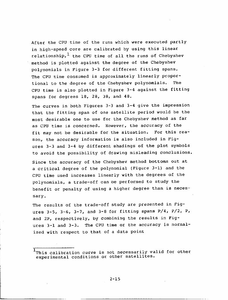
After the CPU time of the runs which were executed partly

in high-speed core are calibrated by using this linear

relationship, 1 the CPU time of all the runs of Chebyshev

method is plotted against the degree of the Chebyshev

polynomials in Figure 3-3 for different fitting spans.

The CPU time consumed is approximately linearly propor-

tional to the degree of the Chebyshev polynomials. The

CPU time is also plotted in Figure 3-4 against the fitting

spans for degrees 18, 28, 38, and 48.

The curves in both Figures 3-3 and 3-4 give the impression

that the fitting span of one satellite period would be the

most desirable one to use for the Chebyshev method as far

as CPU time is concerned. However, the accuracy of the

fit may not be desirable for the situation. For this rea-

son, the accuracy information is also included in Fig-

ures 3-3 and 3-4 by different shadings of the plot symbols

to avoid the possibility of drawing misleading conclusions.

Since the accuracy of the Chebyshev method bottoms out at

a critical degree of the polynomial (Figure 3-1) and the

CPU time used increases linearly with the degrees of the

polynomials, a trade-off can be performed to study the

benefit or penalty of using a higher degree than is neces-

sary.

The results of the trade-off study are presented in Fig-

ures 3-5, 3-6, 3-7, and 3-8 for fitting spans P/4, P/2, P,

and 2P, respectively, by combining the results in Fig-

ures 3-1 and 3-3. The CPU time or the accuracy is normal-

ized with respect to that of a data point

iThis calibration curve is not necessarily valid for other

experimental conditions or other satellites.

2-15

10

"_ 6 -

E"' 5

I-:3O._j

4

3 -

0

GEOS-3

I

P

FITTING SPAN =4

10

I I20 30

DEGREE OF CHEBYSHEV POLYNOMIALS

4O

*EXECUTED ON THE IBM S/360-75 C1 COMPUTER

O• [_R [MAX > 0.35 m• V• []

(I) 0.2 m > I_RIMA x > 0.1 mv I _"

0.35 m > I&RIMA x >0.2 m

.---dl,

0.1 m > ],_R IMA X

P

Figure 3-3. CPU Time Versus Degree of Chebyshev Polynomialsfor Various Fitting Spans for GEOS-3

2-16

.=_E

v

UJ

p.::)Q..rj

lO

GEOS-3

, I , I0 1 2

,FITTING SPAN (PERIODS)

*EXECUTED ON THE IBM S/360-75 C1 COMPUTER

t,I -. "II IARIMAX>0"35m []V 0.35m>IARIMAX >0.2m

iD 0.2 m > IARIMA x > 0.1 m 0.1 m > IARIMA x

[] Z

0

0

Figure 3-4. CPU Time Versus Fitting Span for Various Degrees

of Chebyshev Ploynomials for GEOS-3

2-17

4OO

30O

v

UJ

_o 200

zLu

n-WO.

LU

.J 100uJE

--100

I I

GEOS-3

PFITTING SPAN = "_"

II

IAR I .-- IAR II max, I max, 13

I I_'R Imax, 13

IIIIIIIII

0IIIII --0-- 0-- 0--0

(CPU)i--(CPU) 13

(CPU)13

o

O

I I I I0 10 20 30 40 50

DEGREE OF CHEBYSHEV POLYNOMIALS

Figure 3-5. Changes in Relative Accuracy and Efficiency for

a Fitting Span of P/4 for the GEOS-3 Orbit

2-18

UJ

I-ZUJo

LU

Ud

I-

..J

u3n-

4OO

300

200

100

-100

l I I" III

I GEOS-3

!I E ITTING SPAN=P/2

I

IIII!!

I'_Rlmax. i--lARImax, 18 /

IA Rtmax, 18

,I

I

I I I I

0

10 20 30 40 50

DEGREE OF CHEBYSHEV POLYNOMIAL

Figure 3-6. Changes in Relative Accuracy and Efficiency for

a Fitting Span of P/2 for the GEOS-3 Orbit

2-19

400

300

A

w 200

I-ZLU

n"LUO.W

I-"100

UJ

n.-

-100

I

I'_R!max, i-_Rlmax, 24

I_--"_lmax, 24

1

IIIIIIIIIIIIII

I

GEOS-3

FITTING SPAN=P

(CPU)i_(CPU)24 /

! _

-'o ...... o ...... o

10 20 30 40 50

DEGREE OF CHEBYSHEV POLYNOMIALS

Figure 3-7. Changes in Relative Accuracy and Efficiency for

a Fitting Span of P for the GEOS-3 Orbit

2-20

4OO

30O

UJ

20C<I-zLUt_n.-uJt'L

IM

I-<-_ 100ILl

n,-

--IO00

i I

GEOS-3 |I

FITTING SPAN=2P |ItI!tI!IIIII!

I=_Rlmax, i-lARImax, 40 |

I_Rlmax, 40

!

!I!!!

(CPU)i-(CPU)40 |I

=

I I I I10 20 30 40

DEGREE OF CHEBYSHEV POLYNOMIAL

=o

5O

Figure 3-9. Changes in Relative Accuracy and Efficiency for

a Fitting Span of 2P for the GEOS-3 Orbit

2-21

corresponding to the critical degree of the polynomial on

the saturated portion of the accuracy curve. For example,

the CPU time used in a computer run for fitting a

Chebyshev polynomial of the ith degree over a span of P/4

is normalized with respect to the CPU time consumed for

fitting 13th-degree Chebyshev polynomials over the same

span, i.e.,

[(CPU) i- (CPU)I3]/[(CPU)I3]

Likewise, the accuracy of the fit is also normalized with

respect to the 13th-degree Chebyshev polynomials, i.e.,

(IA lmax,i- IA lmax,13)/(IA lmax,13 )

For the fitting span of P/4, CPU usage doubles without any

benefit at all when the degree is increased from 13th to

25th. Actually, the accuracy has deteriorated by about

i0 percent. If the degree is reduced from 13th to 12th,

the CPU consumption saved is only 0.6 percent, but the

penalty is a significant 70 percent decrease in accuracy.

Therefore, it is very desirable to predefine the require-

ment for support to be accuracy-bound or CPU-bound for

selecting the fitting span and the degree of the Chebyshev

polynomials. An arbitrary combination of these parameters

may either produce an ephemeris with accuracy so poor that

it is not usable or consume more computer resources than

necessary.

Another area of trade-off consideration is whether support

is accuracy-bound or storage-bound. The total number of

Chebyshev coefficients is directly proportional to the

degree of the Chebyshev polynomials and inversely

2-22

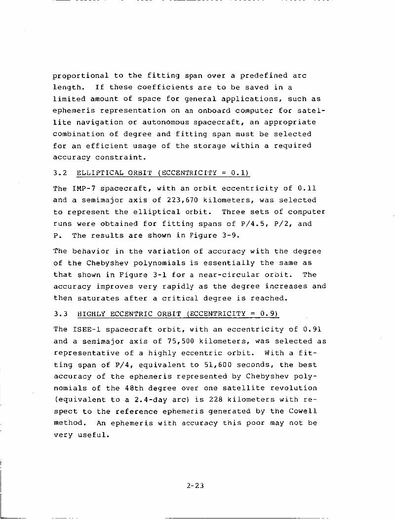
proportional to the fitting span over a predefined arc

length. If these coefficients are to be saved in alimited amount of space for general applications, such as

ephemeris representation on an onboard computer for satel-

lite navigation or autonomous spacecraft, an appropriate

combination of degree and fitting span must be selected

for an efficient usage of the storage within a required

accuracy constraint.

3.2 ELLIPTICAL ORBIT (ECCENTRICITY = 0.I)

The IMP-7 spacecraft, with an orbit eccentricity of 0.ii

and a semimajor axis of 223,670 kilometers, was selected

to represent the elliptical orbit. Three sets of computer

runs were obtained for fitting spans of P/4.5, P/2, and

P. The results are shown in Figure 3-9.

The behavior in the variation of accuracy with the degree

of the Chebyshev polynomials is essentially the same as

that shown in Figure 3-1 for a near-circular orbit. The

accuracy improves very rapidly as the degree increases and

then saturates after a critical degree is reached.

3.3 HIGHLY ECCENTRIC ORBIT (ECCENTRICITY = 0.9)

The ISEE-I spacecraft orbit, with an eccentricity of 0.91

and a semimajor axis of 75,500 kilometers, was selected as

representative of a highly eccentric orbit. With a fit-

ting span of P/4, equivalent to 51,600 seconds, the best

accuracy of the ephemeris represented by Chebyshev poly-

nomials of the 48th degree over one satellite revolution

(equivalent to a 2.4-day arc) is 228 kilometers with re-

spect to the reference ephemeris generated by the Cowell

method. An ephemeris with accuracy this poor may not be

very useful.

2-23

n-U.I

I-uJ

x<

0I-

1.1.1>z0t--

0n

z

iii¢.Jzi.iJn,-wi1

U.

<

1011

10

.01

I

IMP-7ELLIPTICAL ORBIT

(e = 0.11)

H = FITTING SPAN

P - SATELLITE PERIOD

H=IP

P

P

4.5

I I I I I10 20 30 40 50

DEGREE OF CHEBYSHEV POLYNOMIALS

O0o

Figure 3-9. IMP-7 Ephemeris Accuracy for the Chebyshev Poly-nomial Fit Compared With the Cowell Method

2-24

Further tests were conducted with drastically reduced fit-

ting spans of P/40 and P/80. The results are presented in

Figure 3-10. The accuracy obtained was comparable to thatshown in Sections 3.1 and 3.2. As in the cases of cir-

cular orbit and elliptical orbit, theaccuracy curves show

the similar behavior in the variation of accuracy with the

degree of the Chebyshev polynomials.

3.4 AN EMPIRICAL FORMULA TO DETERMINE THE OPTIMAL FITTING

SPAN

Ideally, in applying the Chebysnev method, one would like

to obtain the highest accuracy with a minimum amount of

CPU time for the lowest possiDle degree and the longest

possible fitting span. However, so straightforward an

application is not possible because those factors compete

with each other in a rather complicated fashion as demon-

strated in Sections 3.1, 3.2, and 3.3. An attempt was

made to find an empirical formula for determining an opti-

mal fitting span in terms of satellite period.

From Figures 3-1, 3-9, and 3-10, it is obvious that a

longer fitting span requires a higher degree for the

Chebyshev polynomials in order to achieve acceptable fit-

ting accuracy, i.e., the fitting span should be propor-

tional to the degree of the Chebyshev polynomials. Fur-

thermore, the fitting span must be substantially smaller

for a highly eccentric orbit than for a circular orbit.

From these arguments, a very crude empirical formula re-

sults:

2H = C ° DP (i - e) (3-1)

where H = the fitting span of Chebyshev polynomials in

terms of satellite period

2-25

100

10

rrW

p.w

x<

F0

(.}w>

z0C-

oa.

z

w

Z .1I.U

ccUJu.

u_

x

.01

.001

ISEE-1HIGHLY ELLIPTICAL ORBIT

(e = 0.91 )

H = FITTING SPAN

P = SATELLITE PERIOD

PH

4O

P

8O

I I I

10 20 30 40

DEGREE OF CHEBYSHEV POLYNOMIALS

_0

oco

Figure 3-i0. ISEE-1 Ephemeris Accuracy for the Chebyshev

Polynomial Fit Compared With the Cowell Method

2-26

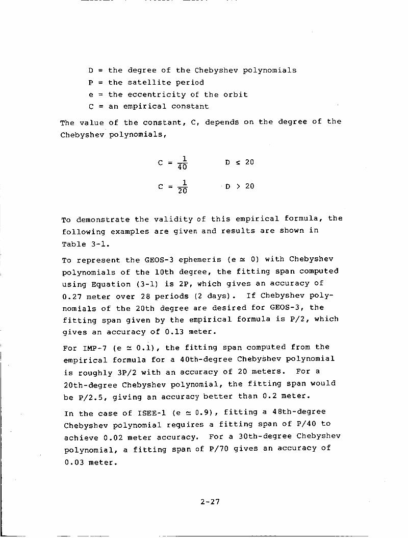
D = the degree of the Chebyshev polynomials

P = the satellite period

e = the eccentricity of the orbitC = an empirical constant

The value of the constant, C, depends on the degree of the

Chebyshev polynomials,

C - 1 D _ 2040

C - 1 D >2020

To demonstrate the validity of this empirical formula, the

following examples are given and results are shown inTable 3-1.

To represent the GEOS-3 ephemeris (e--_ 0) with Chebyshev

polynomials of the 10th degree, the fitting span computedusing Equation (3-1) is 2P, which gives an accuracy of

0.27 meter over 28 periods (2 days). If Chebyshev poly-

nomials of the 20th degree are desired for GEOS-3, thefitting span given by the empirical formula is P/2, which

gives an accuracy of 0.13 meter.

For IMP-7 (e _- 0.i), the fitting span computed from the

empirical formula for a 40th-degree Chebyshev polynomial

is roughly 3P/2 with an accuracy of 20 meters. For a

20th-degree Chebyshev polynomial, the fitting span would

be P/2.5, giving an accuracy better than 0.2 meter.

In the case of ISEE-I (e __0.9), fitting a 48th-degree

Chebyshev polynomial requires a fitting span of P/40 toachieve 0.02 meter accuracy. For a 30th-degree Chebyshev

polynomial, a fitting span of P/70 gives an accuracy of

0.03 meter.

2-27

09/09_'L

-,.-I

"OO

-,.4E

O

c,'j

r.o

4-_.,-t

O

0

r..)_Q

-,-I

•,-! -H

EE_

,.c: •Q_..c:

I

,--'1

,.Q

I-.

n-O

n-

LUO

ILl

>---1"r"

"r"

I--

--I<

I--

J

i--

n-O

n..<

D

n.-

n.-

Z

uJLu

xLU1--

-.I"1I--

O

I.n,O

_.. ,-:.o

0o

o IuJ O

>-

o -_LU l--m

_. z

uJ

0

o

0

0

i_-

Ir'-

CN _v

f CO _.0 A

v

0 _l _ 6

>w

w

z-_ _

:=-I.-

ZZLU

ot-

<..J

o.rk-

_1._1w

o0

oI-I--

I.A.I

fr

'rI--

<

<

00<

2-28

The empirical formula is applied to the Tracking and Data

Relay Satellite (TDRS) and the results are also included

in Table 3-1. The TDRS is to be a geosynchronous satel-

lite with an eccentricity of nearly zero and a semimajor

axis of 42,000 kilometers. The fittihg span computed from

the empirical formula for a 20th-degree Chebyshev poly-

nomial is P/2 which gives an accuracy of 0.14 meter for

the ephemeris over a 31-day arc of 31 revolutions. If a

40th-degree Chebyshev polynomial is chosen, the computed

fitting span is 2P which gives an accuracy of 0.16 meter

over the same arc length.

To further verify the validity of the empirical formula, a

nonexistent Satellite-X with an eccentricity of 0.5 and a

semimajor axis of 13,200 kilometers was tested. The peri-

gee height is 6,600 kilometers, about 200 kilometers above

the surface of the Earth, and the apogee height is

19,800 kilometers. The relati;e importance of all per-

turbing forces, such as a higher-order harmonic geopoten-

tial field, atmospheric drag, and solar radiation

pressure, exerted on Satellite-X varies at different

positions on the orbit causing the magnitude of the

trajectory variation to differ along the orbit. Near the

perigee, a shorter fitting span and a higher degree of

Chebyshev polynomials may be needed to meet required

accuracy criteria because of the effects of a higher-order

harmonic geopotential field and the atmospheric drag.

Near the apogee, a medium fitting span and medium degrees

of the Chebyshev polynomials may be required because of

the large curvature of the trajectory in combination with

the trajectory variation due mainly to the solar radiation

pressure. While in the vicinities of 90 degrees and

270 degrees of anomaly of the orbit, the trajectory is

rather linear and a lower degree and a longer fitting span

may be sufficient. It is not possible, however, to apply

2-29

several different fitting spans and degrees over each

revolution in a single computer run setup with the current

GTDS, which only allows a uniform fitting span and a sin-

gle choice of degree for the Chebychev polynomials.

Two test runs were made with fitting spans of P/8 and P/2

computed by using the empirical formula, Equation (3-1),

for Chebyshev polynomials of the 20th and 40th degrees,

respectively. The accuracy for a P/8 fitting span with a

20th-degree Chebyshev polynomial is 0.55 meter, and

0.62 meter for a P/2 fitting span with a 40th-degree poly-

nomial over a two-day arc of 11.5 revolutions.

With the exception of the case of the 40th-degree poly-

nomial with a 3P/2 fitting for IMP-7, all the cases seem

to favorably support the validity of the empirical for-

mula. However, the formula still should be used with ex-

treme caution, perhaps only as.a rough guideline to

establish a preliminary set of parameters for the

Chebyshev ephemeris generation method.

2-30

SECTION 4 - CONCLUSIONS

The Cheoyshev ephemeris generation method is reimplemented

in the operational version of GTDS. The conclusions from

the testing results for this new implementation are sum-

marized below.

• The new implementation is more efficient and pro-

duces more accurate ephemerides.

• The accuracy of the ephemeris generated by the

Chebyshev method increases with the degree of the

Chebyshev polynomials very rapidly but bottoms

out after a critical degree is reached.

• The accuracy is generally better for smaller fit-

ting spans.

• The efficiency of the Chebyshev method is mainly

related to the degree of the Chebyshev polynom-

ials and the fitting span.

• The Chebyshev method is slower than the Cowell

method. Unless Chebyshev coefficients are re-

quired, the Chebyshev method is not recommended

for use in general applications. A study is cur-

rently underway to further improve the efficiency

of the Chebyshev method by using the Brouwer-

Lyddane theory instead of the two-body theory for

the starter.

• A preliminary empirical formula was deduced to

determine an optimal fitting span with a desir-

able degree of Chebyshev polynomials in terms of

high accuracy of the satellite ephemeris and low

consumption of computer resources.

2-31

It is also recommended that the conclusions of

any study involving the use of Chebyshev ephem-erides obtained from the previous version of GTDSshould be re-evalutated, especially in regard to

accuracy.

2-32

APPENDIX A - MATHEMATICAL THEORY OF THE CHEBYSHEV

ORBIT GENERATION METHOD

A.I PROPERTIES OF CHEBYSHEV POLYNOMIALS

The properties of the Chebyshev polynomials are most

easily examined in the normalized interval [I, -i]. Any

arbitrary finite interval [ta, tb] can be transformed

to the normalized interval [i, -i] by the change of vari-

able: 1

It - t 1=1-2 a

b - _a(A-l)

where = the normalized time variable

t = the start time of a polynomial fitting span,

a (i.e., the start time of an integration step in

GTDS terminology)

t b = the end time of a polynomial fitting span,(i.e., the end time of an integration step and,

therefore,,,t b) - t corresponds to the"step size a

The Chebyshev polynomials are defined as a set of poly-

nomials

T. (_) =.cos i0 i = 0, i, ... (A-2)1

iThe transformation could have been defined as

_= 2 a - 1

b -

so that t a would correspond to -i, and t b would corre-

spond to +i. Since Reference 1 and the GTDS software have

consistently used the definition as shown in Equa-

tion (A-l), this transformation is retained throughout

this document and the new software.

2-33

generated from the sequence of cosine functions using thetransformation

e = cos-l_ -i < _ < 1 (A-3)

Clearly for the zeroth degree

T 0(_) = cos (0) = 1 (A-4)

and for the first degree

TI(_) = _ (A-5)

By repeated trigonometric manipulations, higher-degree

Chebyshev polynomials can be computed yielding the recur-

sion relation

Ti(_) = 2_Ti_l(_) - Ti_2(_) i = 2, 3, ... (A-6)

Table A-1 contains the first ten Chebyshev polynomials.

With simple algebraic manipulation, the algebraic func-

tions, _n, can be expressed in terms of a linear

combination of the Chebyshev polynomials. This is shown

in Table A-2. All the Chebyshev polynomials have a maxi-

mum magnitude of 1 in the interval [i, -i]. The Chebyshev

polynomials of degrees 0 to 3 are plotted in Figure A-I.

The function of a parabola, _2, is also plotted in the

figure as a linear combination of T 0 and T 2. Except

for T0, all other Chebyshev polynomials cross the

_-axis. The number of times that axis is crossed is equal

to the degree of the Chebyshev polynomial and only those

2-34

Table A-I. The Chebyshev Polynomials

T0=I

T 1 =_

T 2 = 2 E2 _ 1

T3=4_3--3_

T4=8_'4--8_2 + 1

T5= 1655-- 20 _3+55

T6=32_6-4854+18_'2_ 1

T 7=64_7- 112_5+56_3--71_

T 8= 12858-256_6+160_4_32_2+1

T 9 =256 $9 _ 576 t_7+ 432 t_5 - 120 _3 + 9

2-35

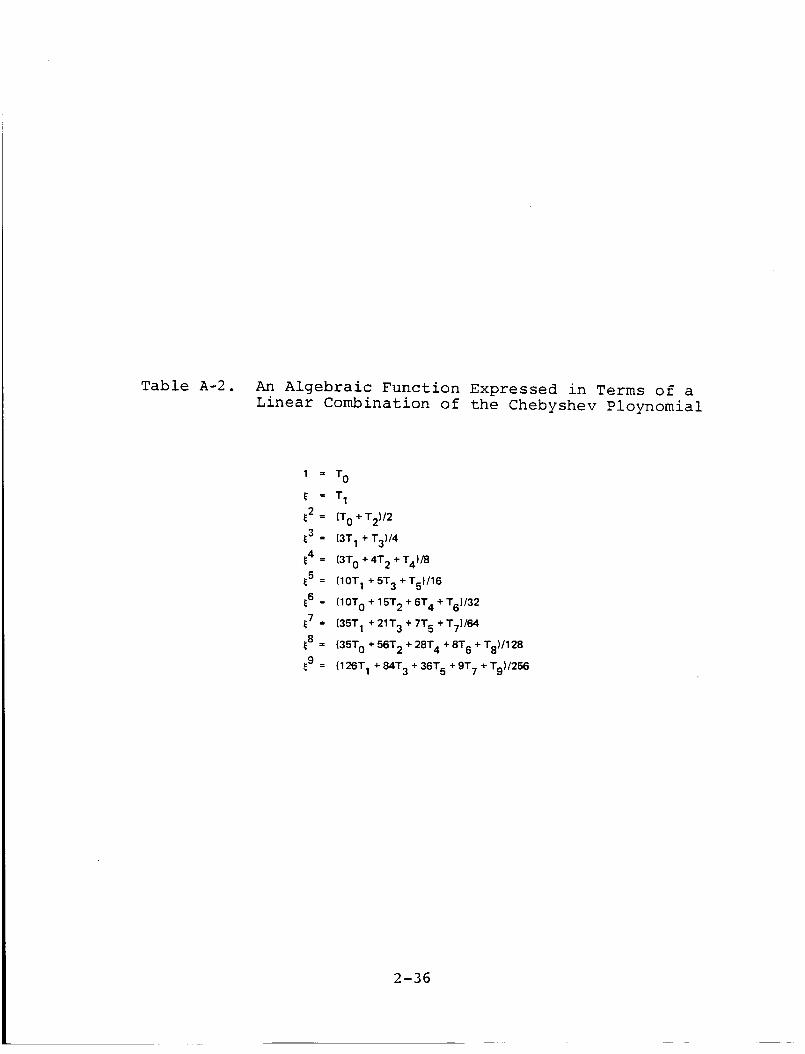
Table A-2. An Algebraic Function Expressed in Terms of a

Linear Combination of the Chebyshev Ploynomial

1 = T O

/_ = T 1

_2 = (T 0+T2)/2

_3 = (3T1 + T3)/4

_4 = (3T0 +4T 2 +T4)/8

_5 = (10T 1 + 5T 3 + T5)/16

_6 = (10T 0+15T 2+6T 4+T 6)/32

_7 = (35T 1 + 21T3 + 7T 5 +T7)/64

_.8 = (35T 0 + 56T2 + 28T4 + 8T 6 + T8)/128

_9 = (126T 1 ÷ 84T 3 + 36T 5 + 9T 7 + T9)/256

2-36

L

-1

Figure A-I. Chebyshev Polynomials of Degrees 0 to 3

2-37

of odd degrees will cross the origin. The n locations at

which the Chebyshev polynomial Tn(_) crosses the _-axis

are the n roots in the interval [i, -i] and are given by

_k = Icos (2k2n- i)_ 1k = i, ..., n (A-7)

The significant properties of using the Chebyshev poly-

nomials to fit an arbitrary function are that the error in

the approximation is distributed evenly over the interval

and the maximum error is reduced to the minimum or near-

minimum value (References 3 and 4).

A.2 INTERPOLATING POLYNOMIALS CONSISTING OF A LINEAR

COMBINATION OF CHEBYSHEV POLYNOMIALS OF DIFFERENT

DEGREES TO REPRESENT ACCELERATION

Each component of the acceleration vector exerted on the

spacecraft can be approximated by an interpolating poly-

nomial consisting of a linear combination of Chebyshev

polynomials:

n

_(_) : Pn(_): _ CiTi(_) (A-8)i=0

where _ = the Cartesian component of the acceleration

vector

Pn = the interpolating polynomial of degree n

C i = Chebyshev coefficients for an accelerationcomponent

= the transformed time variable

The accuracy of this approximation is better when the

higher degrees of Chebyshev polynomials are included.

However, the benefit of including higher degrees drops off

quickly. This point is further illustrated in Section 4.

2-38

It is well known that the Chebyshev polynomials are one of

the families which possess the property of orthogonality(References 3 and 4). They are orthogonal in the interval

[i, -i] with respect to the weighting function,

w(_) =i/ /i- _2, i.e.,

_ i i1 i - _2 Ti(_) Tj(_) d_ = 0, i _ j

_-.i_;1 1 IT i(6)] 2 d_ = A _ 01 /l - _2 i

(A-9)

where A. is a normalization factor which depends on i.1

Making use of the property of orthogonality, as demon-

strated in Equation (A-9), the Chebyshev coefficients can

be evaluated

1 /_i I 1 Ti(_ ) _(_)Ci = _ii /i- _ 2

i = 0, i, ..., n

d_

(A-10)

The above integral is difficult to evaluate because of the

complexity of _(_). However, it has been shown (Refer-

ences 3, 4, and 5) that Equation (A-10) may be approxi-

mated by

n+l

_ 1 )CO n + 1k=l

n+l

C : 2 _ Ti(_k)_(_k )i n + 1k=l

i = i, 2, • --r n

(A-If)

2-39

where _k are the roots of the Chebyshev polynomial of

degree n + i, Tn+l(_). Therefore, with the accelera-tions evaluated at all the n + 1 roots, the variation of

the acceleration in the interval [i, -i], corresponding to

the time interval [ta, tb] , can be represented by the

interpolating polynomial, Pn(_) , of degree n.

A.3 INTEGRATION OF CHEBYSHEV INTERPOLATING POLYNOMIAL TO

GENERATE EPHEMERIS

With the acceleration components represented by Chebyshev

interpolating polynomials as shown in Equation (A-8), in-

tegrating the equation once gives the velocity compo-

nents, _:

_(_) = n(_) d_ = _ C i Ti(_) d_ (A-12)i=0

Through the use of Equations (A-4), (A-5), and (A-6), the

integration of the Chebyshev polynomials of different de-

grees can be obtained:

T0(_) d_ = TI(_) + K 0

/ ]TI(_) d_ = _ 0(_) + T2(_) + K 1

Ti(_) d_ = i + 1 Ti+l(_) 1 Ti (_)]i - 1 -i

i = 2, 3, ..., n

+ K i ,

(A-13)

where K0, KI, and K i are integration constants.

2-40

Substituting Equation (A-13) into Equation (A-12) and col-

lecting terms of Chebyshev polynomials of the same degreesyields another interpolating polynomial of the following

form for the velocity components:

n+l

x(_) = /Pn(_) d_ = Qn+l(_) = i=0_ b i Ti(_) (A-14)

where Qn+l = the interpolating polynomial of degree n + 1

b = Chebyshev coefficients for a velocity compo-

1 nent

with

C 1

b 0 = K 0 + K 1 + ... + _--T O

1

b I = C O - _ C2

Cn+ 1 = Cn+ 2 = 0

2, 3, ..., n + 1

(A-15)

The integration constants in the expression for b 0 may

be evaluated from the initial velocity, i.e., X(ta) =

i):

I) -n+l

i=lb. T. (_ = i) = b 0 T0(_ = i) = b 01 1

(A-16)

2-41

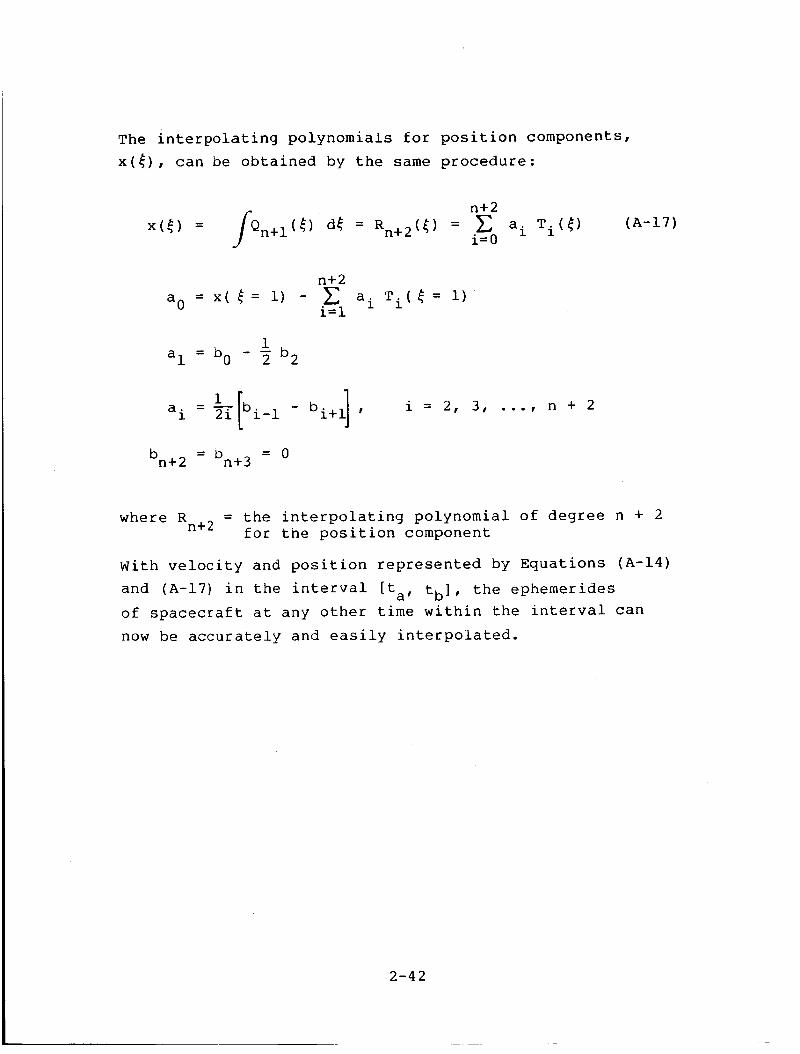
The interpolating polynomials for position components,

x(_), can be obtained by the same procedure:

n+2

x(_) = /Qn+l(_) d_ = Rn+2(_) = i=0_ a i Ti(_)(A-17)

a 0 = x( _ = i) -

1

a I = b 0 - _ b2

n+2

a i T.(_=l I)i=l

a i = _-{ bi_ 1 - bi+ ,

bn+ 2 = bn+ 3 = 0

i = 2, 3, ..., n + 2

= the interpolating polynomial of degree n + 2where Rn+ 2 for the position component

With velocity and position represented by Equations (A-14)

and (A-17) in the interval [ta, tb], the ephemerides

of spacecraft at any other time within the interval can

now be accurately and easily interpolated.

2-42

APPENDIX B - COMPARISON BETWEEN THE IMPROVED IMPLEMENTATION

AND THE PREVIOUS IMPLEMENTATION OF THE CHEBYSHEV METHODS

A series of GTDS computer runs was executed to compare the

new and the previous software implementations in terms of

their accuracy and efficiency. The accuracy was measured

with respect to the ephemeris generated with the high-

precision Cowell numerical integration method by using the

GTDS Ephemeris Comparison Program. The efficiency is sim-

ply a comparison of the CPU and I/O times consumed by the

two different Chebyshev implementations.

Three sets of test runs were made on GTDS with the GEOS-3

satellite (arbitrarily chosen) over a two-day span using

the Cowell method and the Chebyshev polynomial method of

the new and previous implementations. The comparison

results are presented in Table B-I. In these tests, the

ephemeris generated by the Cowell integration method with

a 24-second step size was used as a reference. The per-

turbation (or force model) included in the Cowell method

was identical to that used in the Chebyshev methods.

Table B-I shows that the maximum difference in position

vector of the ephemeris generated by the previous

Chebyshev implementation with a 48th degree polynomial

over a two-day arc is 97 meters with respect to the

ephemeris generated by the Cowell method, while the new

Chebyshev implementation with the same degree of poly-

nomial has a maximum position difference of only

0.25 meter. This represents an improvement of better than

two orders of magnitude in the relative accuracy.

The efficiency which is expressed as CPU time and I/O time

consumed on the IBM S/360-75 computer is also examined.

2-43

0-,-I

.IJr_44

0

0f-I

I.-I

>

o"o•,-I 0

_,--4

_o

Z

_o

L)

0

.,-I

E.p0",-I

I

,-I

r_

O_mW

_ww_

_0_

,'7 _. 0

$

u.><0 w-

w>° z_00

w'r

r_0-,rI-,11

_±>_--

O_W

<_Ow

2z__-_w_w

m

0

R0

F_

0

"7o

z0m-<k-zw

e_

ILl

z

z0

mzDwO_--W

J<

_.-0O_

OzuJDc3_n

X

z0I-,<i-z14.1

14.1

.J_6

:E

z

oz w

z" J___

Ow ;<z

x_ ,_0_m,,- _ :E n"

0_1

/

0

w< n"

I.U

>-<

_- co"ILl

> >-0

-- D

w

o_ o ,,

I I--i1,1O:E D __-,.

141"I"I-n"0IL

oz0

u.i£0

Z<

0k-<n-

U.I

z

I-

r_0>ILl

7"

>-a214.1"t-OILl"r"

n-Ou_

oz0

uJ

0

w

N

0.

I-

_ .

O0

w _ _ ,_

o _ n- g

- = z2 _z_

w

¢_I _ II II II II II II iii_

, w _ ..t- 0x I- (_ _ _ .- _ 3 _ i--O

_ w _

2-44

The previous implementation used 8.012 minutes of CPU timeand 0.154 minute of I/O time, while the new implementation

used only 5.806 minutes of CPU time, a saving of 38 per-

cent, and a comparable 0.142 minute of I/O time.

The saving of computer resources can be viewed from

another angle by lowering the degree of Chebyshev poly-nomials from 48 to 20 and 18. The results are also shown

in Table B-I. Fitting Chebyshev polynomials with much

lower degrees, the new implementation consumes four tofive times less CPU resources yet maintains better ac-

curacy than the previous implementation.

Results in Table B-I indicate similar conclusions with

more elaborate perturbation models, i.e., 8x8 geopotential

field, 14th order resonance geopotential field, atmos-

pheric drag, and solar radiation pressure as well as solar

and lunar gravitational fields.

The results presented in Table B-I are obtained with a

fitting span of one satellite period for both the new andprevious implementation. When the fitting span is in-

creased to two satellite periods, the new implementation

gives excellent results (I ARlmax = 0.12 meter) . How-ever, after 80 loops in the iterative scheme, the previous

implementation has simply failed to satisfy the10 -6 kilometer tolerance in fitting the first span and

the computer run was subsequently terminated without gen-

erating an ephemeris.

2-45

io

REFERENCES

Goddard Space Flight Center, X-582-73-176, Description

of the Numerical Integration of the Equations of Mo-

•

•

•

•

tion of a Space Vehicle Using Chebyshev Series,

T. Feagin, June 1973

Goddard Space Flight Center, X-582-76-77, Mathematical

Theory of the Goddard Trajectory Determination System

(GTDS), J. O. Capellari, C. E. Velez, and A. J. Fuchs,

April 1976.

Fox, L., and I. B. Parker, Chebyshev Polynomials in

Numerical Analysis• London: Oxford University Press,1972.

Carnahan, B., H. A. Luther, and J. O. Wilkes, Applied

Numerical Methods. New York: John Wiley and Sons,

Inc., 1969

Snyder, M. A., Chebyshev Methods in Numerical Approxi-

mation• Englewood Cliffs, New Jersey: Prentice-Hall,1966

2-46