ABSTRACT HIGHLY EXTENSIBLE SKIN FOR A VARIABLE WING …

ABSTRACT

Title of Thesis: HIGHLY EXTENSIBLE SKIN FOR A VARIABLE

WING-SPAN MORPHING AIRCRAFT UTILIZING

PNEUMATIC ARTIFICIAL MUSCLE

ACTUATION.

Edward A. Bubert, Master of Science, 2009

Thesis Directed By: Professor Norman M. Wereley

Department of Aerospace Engineering

Two different technologies are demonstrated for a span-morphing wingtip: a linear

controller for a pneumatic artificial muscle (PAM) actuator, and a passive 1-D morphing

skin. A generic PAM system incorporating a single PAM working against a nonlinear

spring is described in a Simulink model, which is validated using experimental data. A

linear PID controller is then incorporated into the model. Frequency responses are

obtained by both simulation and experiment, and the ability to track relatively high

frequency control inputs is demonstrated. The morphing skin system includes an

elastomer-fiber-composite surface layer that is supported by a flexible honeycomb

structure, each of which exhibit a near-zero in-plane Poisson’s ratio. Composite skin and

substructure configurations are designed using analytical methods and downselected after

experimental evaluation. A complete prototype morphing skin, mated to a PAM driven

extension mechanism, demonstrates 100% uniaxial extension accompanied by a 100%

increase in surface area. Out-of-plane deflections under surface pressures up to 200 psf

(9.58 kPa) are reported at varying levels of area change.

HIGHLY EXTENSIBLE SKIN FOR A VARIABLE WING-SPAN

MORPHING AIRCRAFT UTILIZING PNEUMATIC ARTIFICIAL

MUSCLE ACTUATION.

By

Edward A. Bubert

Thesis submitted to the Faculty of the Graduate School of the

University of Maryland, College Park, in partial fulfillment

of the requirements for the degree of

Master of Science

2009

Advisory Committee:

Professor Norman M. Wereley, Chair

Professor Christopher Cadou

Professor J. Sean Humbert

ii

Acknowledgments

I would like to begin by thanking my advisor, Dr. Norman Wereley, who has been a

reliable source of knowledge and guidance, and the other members of my graduate

committee, Dr. Christopher Cadou and Dr. Sean Humbert, for their advice and help in

preparing this thesis.

Much of the work presented here was done with the support of Techno-Sciences, Inc.

under Dr. Peter Chen. Additional thanks go to Dr. Curt Kothera for his invaluable

assistance during testing and analysis.

For the work in Chapter 3, sponsorship was provided by the Air Force Research

Laboratory (AFRL) through a Phase I STTR, contract number FA9550-06-C-0132. I

would like to thank technical monitors Drs. Brian Sanders and Victor Giurgiutiu for their

contributions.

Finally, I would like to thank my friends and coworkers at the University of Maryland,

in particular Ben Woods, Robert Vocke, and Michael Gentry, for help in all aspects of

executing this research.

iii

Table of Contents

ABSTRACT......................................................................................................................... i

Acknowledgments............................................................................................................... ii

Table of Contents............................................................................................................... iii

List of Figures ......................................................................................................................v

List of Tables ................................................................................................................... viii

List of Notations ................................................................................................................ ix

Chapter 1: Introduction ........................................................................................................1

1.1 Morphing Overview............................................................................................ 1

1.2 Morphing Skin Review....................................................................................... 2

1.3 Span Morphing Actuation Mechanism ............................................................... 4

1.3.1 PAM Actuators ........................................................................................... 5

1.3.2 Pneumatic Artificial Muscle Control Review............................................. 7

1.3.3 X-Frame Extension Mechanism ................................................................. 9

1.4 Outline of Thesis and Technical Objectives ..................................................... 12

Chapter 2: Pneumatic Actuator System Modeling and Control.........................................14

2.1 Overview........................................................................................................... 14

2.2 SPTA Description ............................................................................................. 14

2.3 SPTA Model Development and Verification.................................................... 20

2.3.1 PAM Force Model .................................................................................... 21

2.3.2 Nonlinear Spring Model ........................................................................... 23

2.3.3 PAM Pressure Model................................................................................ 24

2.3.4 Mass Flow through Valve Orifice............................................................. 26

2.3.5 Valve Area Characterization..................................................................... 27

2.3.6 Effects of Connecting Tubing................................................................... 32

2.3.7 Pneumatic Model in Simulink .................................................................. 34

2.3.8 Full SPTA Model in Simulink .................................................................. 39

2.4 SPTA Controller ............................................................................................... 46

2.4.1 SPTA Controller Design ........................................................................... 46

2.4.2 SPTA Controller Results and Analysis..................................................... 47

2.5 SPTA Closed Loop Experimental Results........................................................ 51

2.6 Conclusion ........................................................................................................ 59

Chapter 3: Design and Fabrication of a Passive 1-D Morphing Aircraft Skin ..................61

3.1 Overview........................................................................................................... 61

3.2 FMC Design and Testing .................................................................................. 64

3.2.1 Elastomer Selection .................................................................................. 64

3.2.2 CLPT Predictions and Validation ............................................................. 66

3.2.3 FMC Fabrication and Testing ................................................................... 74

iv

3.3 Substructure Design and Testing ...................................................................... 76

3.3.1 Honeycomb Design................................................................................... 76

3.3.2 Honeycomb Substructure FEM Analysis.................................................. 84

3.3.3 Carbon Fiber Stringers.............................................................................. 85

3.3.4 FMC/Substructure Adhesive..................................................................... 86

3.4 Integration and Final Testing ............................................................................ 89

3.4.1 In-Plane Testing ........................................................................................ 92

3.4.2 Out-of-Plane Deflection............................................................................ 93

3.4.3 Full-Scale Integration and Evaluation ...................................................... 96

3.5 Conclusions....................................................................................................... 99

Chapter 4: Conclusions and Future Work........................................................................101

4.1 Summary of Research and Technical Contributions ...................................... 101

4.1.1 PAM Actuator Controller ....................................................................... 101

4.1.2 Morphing Skin ........................................................................................ 102

4.1.3 Technical Contributions.......................................................................... 103

4.2 Future Work .................................................................................................... 104

Chapter 5: References ......................................................................................................106

v

List of Figures

Fig. 1: Span-morphing UAV showing 1-D morphing wingtips ......................................... 2

Fig. 2: Pneumatic artificial muscle ..................................................................................... 5

Fig. 3: Typical PAM load line characterization.................................................................. 6

Table 1: Results of selected pneumatic actuator control studies ........................................ 8

Fig. 4: PAM-driven x-frame actuation mechanism concept ............................................... 9

Fig. 5: X-frame design ...................................................................................................... 10

Fig. 6: X-frame testing...................................................................................................... 11

Fig. 7: System performance comparison at 90 psi ............................................................ 12

Fig. 8: Single PAM Test Apparatus.................................................................................. 16

Fig. 9: Pneumatic circuit setup.......................................................................................... 17

Fig. 10: Festo MPYE-5-1/8HF-010-B proportional 5/3-way spool valve........................ 18

Fig. 11: SPTA characterization results ............................................................................. 19

Fig. 12: Free body diagram of spring plate assembly....................................................... 20

Fig. 13: High order polynomial fits to SPTA PAM data .................................................. 22

Fig. 14: Spring force characterization............................................................................... 23

Fig. 15: PAM volume measurement device...................................................................... 25

Fig. 16: Volume measurement device for SPTA PAM .................................................... 26

Fig. 17: Steel pressure vessel for spool valve characterization. ....................................... 28

Fig. 18: 5/3-way spool valve operation............................................................................. 28

Fig. 19: Port 2 flow characterization showing valve area fit results................................. 30

Fig. 20: Festo MPYE 5/3-way spool valve characterization results................................. 32

Fig. 22: Tubing loss model comparison, 4” tubing, 1 Hz, low flow................................. 36

Fig. 23: Tubing loss model comparison, 4” tubing, 1 Hz, high flow ............................... 36

Fig. 24: Tubing loss model comparison, 4” tubing, 7 Hz, high flow ............................... 37

Fig. 25: Tubing loss model comparison, 24” tubing, 1 Hz, low flow............................... 38

Fig. 26: Tubing loss model comparison, 24” tubing, 1 Hz, high flow ............................. 38

Fig. 27: Tubing loss model comparison, 24” tubing, 7 Hz, high flow ............................. 39

Fig. 28: Full SPTA System Simulink block diagram ....................................................... 40

Fig. 29: PAM block diagram showing orifice flow block and PAM force block............. 41

Fig. 30: PAM Force block diagram .................................................................................. 41

vi

Fig. 31: SPTA model predictions, 1 Hz sine input ........................................................... 43

Fig. 32: SPTA model predictions, 7 Hz sine input ........................................................... 44

Fig. 33: SPTA model predictions, 14 Hz sine input ......................................................... 45

Fig. 34: Displacement feedback control diagram ............................................................. 46

Fig. 35: Simulated frequency response of PI and PID controllers.................................... 47

Fig. 36: SPTA simulation, controller comparison, 0.1” sine input, 1 Hz ......................... 48

Fig. 37: SPTA simulation, controller comparison, 0.1” sine input, 5 Hz ......................... 48

Fig. 38: SPTA simulation, controller comparison, 0.1” sine input, 15 Hz ....................... 49

Fig. 39: SPTA simulation, controller comparison, 0.1” sine input, 30 Hz ....................... 49

Fig. 40: Prediction of higher order closed loop displacement tracking capability ........... 51

Fig. 41: SPTA closed loop frequency response using PID as compared with model....... 52

Fig. 42: Model PID (top) vs. experiment PID (bottom), 1 Hz.......................................... 53

Fig. 43: Model PID (top) vs. experiment PID (bottom), 5 Hz.......................................... 53

Fig. 44: Model PID (top) vs. experiment PID (bottom), 12 Hz........................................ 54

Fig. 45: Model PID (top) vs. experiment PID (bottom), 24 Hz........................................ 54

Fig. 46: Effect on model of including low pass Butterworth filter at 2 Hz ...................... 56

Fig. 47: Experimental closed loop tracking of higher order harmonic input.................... 57

Fig. 48: Overview of morphing skin conceptual design ................................................... 61

Fig. 49: Proposed morphing skin prototype including PAM actuation system ................ 62

Fig. 50: X-frame force predictions and morphing skin stiffness design goal ................... 63

Fig. 51: Elastomer stress-strain curves ............................................................................. 65

Table 2: Approximate modulus of elastomers .................................................................. 65

Fig. 52: FMC lay-up used in CLPT predictions ............................................................... 66

Fig. 53: Unidirectional composite layer showing fiber orientation .................................. 67

Fig. 54: Comparison of CLPT predictions with experimental data showing effects of

bonding assumptions on solution...................................................................................... 71

Fig. 55: Fiber/matrix bond condition ................................................................................ 72

Fig. 56: Manufacturing a ~1.5 mm FMC.......................................................................... 74

Fig. 57: Lay-ups of FMC samples fabricated for morphing skin evaluation.................... 75

Fig. 58: In-plane skin testing ............................................................................................ 76

Fig. 59: Comparison of standard, auxetic, and modified zero-Poisson cellular structures

showing strain relationships.............................................................................................. 77

Fig. 60: Geometry of zero-Poisson honeycomb cell......................................................... 78

vii

Fig. 61: Forces and moments on bending member leg ..................................................... 78

Fig. 62: Analytical results for substructure in-plane stiffness .......................................... 80

Fig. 63: Example of Objet PolyJet rapid-prototyped zero-Poisson honeycomb............... 81

Fig. 64: Substructure testing ............................................................................................. 82

Fig. 65: In-plane substructure stiffness, analytical versus experiment ............................. 83

Fig. 66: Geometry, boundary conditions and meshes for honeycomb model .................. 84

Fig. 67: Local strain during 30% global compression, max local strain = 1.5%.............. 85

Fig. 68: Reinforced morphing skin cells........................................................................... 86

Fig. 69: Two views of a lap shear test sample .................................................................. 87

Fig. 70: Adhesive lap shear test results, horizontal lines indicate failure......................... 88

Fig. 71: FMC-structure bonding method .......................................................................... 90

Fig. 72: Completed sample, Skin #2................................................................................. 91

Table 3: Morphing Skin Samples, Summary.................................................................... 91

Fig. 73: Morphing skin sample in-plane testing ............................................................... 92

Fig. 74: Contributions to in-plane skin stiffness............................................................... 93

Fig. 75: Out-of-plane deflection test apparatus design ..................................................... 94

Fig. 76: Out-of-plane deflection testing............................................................................ 95

Fig. 77: Out-of-plane deflection results as measured on the center rib ............................ 96

Fig. 78: Integration of morphing cell ................................................................................ 97

Fig. 79: Morphing cell data............................................................................................... 98

viii

List of Tables

Table 1: Results of selected pneumatic actuator control studies. ....................................... 8

Table 2: Approximate modulus of elastomers. ................................................................. 65

Table 3: Morphing Skin Samples, Summary.................................................................... 91

ix

List of Notations

A = proportional spool valve orifice area

[A] = extensional stiffness matrix for orthotropic composite lamina

[B] = coupling stiffness matrix for orthotropic composite lamina

b = depth of honeycomb cell

c = honeycomb cell width

Cd = discharge coefficient for orifice mass flow

C1 = subsonic mass flow term

C2 = supersonic mass flow term

CLPT = Classical Laminated Plate Theory

[D] = bending stiffness matrix for orthotropic composite lamina

Dt = tubing diameter

E = Young’s modulus

Ef = FMC fiber modulus

EL = longitudinal elastic modulus for orthotropic composite lamina

ET = transverse elastic modulus for orthotropic composite lamina

Em = FMC matrix modulus

E0 = honeycomb material elastic modulus

E1 = effective honeycomb elastic modulus

E2 = transverse or spanwise FMC elastic modulus

F = force on honeycomb bending member during extension

f = Moody friction factor for internal flow

Fp = PAM actuator force

x

FMC = Flexible Matrix Composite

GLT = shear modulus for unidirectional composite lamina

h = honeycomb cell height

hk = distance of top of kth lamina from bottom of laminate

hk-1 = distance of bottom of kth lamina from bottom of laminate

I = honeycomb bending member second moment of area

La = length of actuator in x-frame mechanism

Lap = distance of actuator mounting from center of x-frame mechanism

Lt = length of tubing between valve and volume to be filled

Lx = chordwise length of x-frame actuator

Ly = spanwise length of x-frame actuator

LP,0 = PAM resting length

ℓ = length of honeycomb bending member leg

{M} = vector of CLPT laminate in-plane moments

m� = mass flow rate through orifice

delaym� = mass flow rate through orifice, delayed by tubing length

{N} = vector of CLPT laminate in-plane forces

n = number of laminae in FMC composite

P = PAM actuator pressure

PAM = Pneumatic Artificial Muscle

Pcr = critical pressure ratio for orifice flow

PI = proportional-integral linear controller

PID = proportional-integral-derivative linear controller

xi

Pu = upstream pressure in orifice flow calculation

Pd = downstream pressure in orifice flow calculation

[Q] = lamina stiffness matrix in material axes

[ ]Q = lamina stiffness matrix in laminate body axes

R = gas constant for fluid during mass flow

ReD = Reynolds number inside tubing

rd = reference displacement for SPTA linear controller

Rt = resistance in tubing due to fluid viscosity

RTV = Room Temperature Vulcanization

[S] = lamina compliance matrix in material axes

SPTA = Single PAM Test Apparatus

T = ambient temperature

t = thickness of honeycomb bending member

ts = FMC laminate skin thickness

UAV = Unmanned Aerial Vehicle

ud = control input to SPTA proportional valve

V = PAM actuator volume

Vf = FMC lamina fiber volume fraction

α = specific heat constant for fluid undergoing changing volume

αin = approximate specific heat constant for pressure change due to inflow

αout = approximate specific heat constant for pressure change due to exhaust

γ = ratio of specific heats for fluid during orifice mass flow

∆LP = change in PAM length, contraction is positive

xii

∆P = pressure drop along length of tubing

δ = deflection of honeycomb bending bending member

{ε0} = vector of CLPT laminate mid-plane strains

ε = PAM actuator non-dimensionalized contraction

ε1 = global honeycomb strain

θ = angle between honeycomb rib member and bending member

θf = fiber offset angle, measured from chordwise (1) axis

µ = fluid viscosity

ν = honeycomb material Poisson’s ratio

νLT = major Poisson’s ratio of orthotropic composite lamina

ν21 = minor Poisson’s ratio for an FMC laminate

σ1 = effective global honeycomb stress

τ = mass flow time delay due to tubing length

Φ = tubing loss term providing mass flow amplitude attenuation

1

Chapter 1 Introduction

1.1 Morphing Overview

Since the Wright Brothers’ first flight, the idea of changing an airplane’s aerodynamic

characteristics through continuous shape change, rather than discrete flaps or moving

surfaces, has held the promise of more efficient flight. While the Wrights used a

technique known as wing warping, or twisting the wings through structural deformation

to control the roll of the aircraft [1], any number of possible morphological changes could

be undertaken to modify an aircraft’s flight path or overall performance. Some notable

examples include the Parker Variable Camber Wing used for increased forward speed

[2], the impact of a variable dihedral wing on aircraft stability [3], the high speed

dash/low speed cruise abilities associated with wings of varying sweep [4], and the

multiple benefits of cruise/dash performance and efficient roll control gained through

telescopic wingspan changes [5, 6, 7].

While the aforementioned concepts focused on large-scale, manned aircraft, morphing

technology is certainly not limited to vehicles of this size. In fact, the development of a

new generation of unmanned aerial vehicles (UAVs), combined with advances in actuator

and materials technology, has spawned renewed interest in radical morphing

configurations capable of matching multiple mission profiles through shape change – this

class has come to be referred to as “morphing aircraft” [8]. Contemporary research is

primarily dedicated to various wing configuration changes, namely, twist, camber, span,

2

and sweep. It has been shown that morphing adjustments in the planform of a wing

without hinged surfaces leads to improved roll performance, which can expand the flight

envelope of an aircraft [9]. More specifically, morphing to increase the span of a wing

results in a reduction in induced drag, allowing for increased range or endurance [10].

The research presented here is intended for just such a span-morphing application, for

example a UAV with span-morphing wingtips depicted in Fig. 1. By achieving large

changes in the span dimension over a small section of wing, the wing aspect ratio can be

optimized in-flight for different roles. Furthermore, differential span change between

wingtips can generate a roll moment, potentially replacing ailerons on the aircraft [11].

Fig. 1: Span-morphing UAV showing 1-D morphing wingtips.

1.2 Morphing Skin Review

A key challenge in developing a span-morphing wingtip is the development of a useful

morphing skin, defined here as a continuous layer of material that would stretch over the

morphing structure and mechanism to form a smooth aerodynamic skin surface. For a

span-morphing wingtip in particular, the necessity of a high degree of surface area

change, large strain capability in the span direction, and little to no strain in the

3

chordwise direction, all impose difficult requirements on any proposed morphing skin.

The goal of this effort was a 100% increase in both the span and area of a morphing wing

tip, or morphing cell.

A review of contemporary morphing skin technology [12] yields three major areas of

research being pursued: compliant structures, shape memory polymers, and anisotropic

elastomeric skins. Compliant structures such as the FlexSys Inc. Mission Adaptive

Compliant Wing (MACW) rely on an internal structure tailored to deform in a prescribed

manner to allow small amounts of trailing edge camber change [13]. Because only small

deformations are needed, conventional metal or resin-matrix-composite skin materials

can be used to carry aerodynamic loads. Due to the large geometrical changes required

for a span-morphing wingtip as envisioned here, metal or resin-matrix-composite skin

materials are unsuitable because they are simply unable to achieve the desired goal of

100% increases in morphing cell span and area.

Shape memory polymer (SMP) skin materials are relatively new and have recently

received attention for morphing aircraft concepts. They may at first glance seem highly

suited to a span-morphing wingtip: shape memory polymers made by Cornerstone

Research Group [14] exhibit an order of magnitude reduction in modulus and up to 200%

strain capability when heated past a transition temperature, yet return to their original

modulus upon cooling. This would allow a skin to hold its shape under aerodynamic

loads in different morphed positions, yet be made soft enough to morph to new positions

with low actuation forces. There have been attempts to capitalize on the capabilities of

SMP skins, such as Lockheed Martin’s Z-wing morphing UAV concept [15]. However,

electrical heating of the SMP skin to reach transition temperature proved difficult to

4

implement in the wind tunnel test article and the SMP skin was abandoned as a high-risk

option. Additionally, the time required for heating SMP material to transition appears to

make it ill-suited for dynamic control morphing objectives.

With maximum strains above 100%, low stiffness, and a lower degree of risk due to

their passive operation, elastomeric materials are ideal candidates for a morphing skin

[16]. Isotropic elastomer morphing skins have been successfully implemented on the

MFX-1 UAV [17]. This UAV employs a mechanized sliding spar wing structure capable

of altering the sweep, wing area, and aspect ratio during flight. Sheets of silicone

elastomer connect rigid leading and trailing edge spars, forming the upper and lower

surfaces of the wing. The elastomer skin is reinforced against out-of-plane loads by

ribbons stretched taught immediately underneath the skin, which proved effective for

wind tunnel testing and flight testing. Not seen in literature at the start of this research

were any examples of elastomeric skins tailored specifically for span-morphing

applications with a suitable supporting substructure to withstand aerodynamic loads.

1.3 Span Morphing Actuation Mechanism

A complete span morphing wing system would incorporate a morphing skin as well as

a mechanized supporting structure to provide actuation power to the skin surface and

transfer aerodynamic loads to the rest of the wing. Strain capability is once again a

primary motivating factor, with an overall goal of 100% length change. Weight is also a

critical factor in any aircraft design, especially for an actuator system situated at the

wingtip, where the impact on wing root bending moment will be greatest. Background

work focused on the selection and development of a high length change extending

mechanism using a high power density pneumatic artificial muscle actuator [18].

5

1.3.1 PAM Actuators

McKibben actuators, the type of pneumatic artificial muscle (PAM) used in this study,

consist of a rubber bladder surrounded by a braided sleeve attached at each end to rigid

fittings, as seen in Fig. 2. Upon inflation of the bladder by a working fluid (in this case

air), the bladder and braid will expand radially. Because the braid fibers are relatively

stiff and fixed at each end, in order to expand radially the braided sleeve will necessarily

have to contract axially. If unloaded, contraction will continue until the angle between

braid fibers which yields the maximum internal volume is achieved, as in Fig. 2b. This

point corresponds to the minimum energy state, where internal pressure is minimized for

a given mass of air [19]. If contraction is opposed by a load, the pressure within the PAM

will generate axial tension which seeks to return the PAM to the minimum energy state.

This return force is directly proportional to internal pressure and decreases with

contraction ratio (defined here as ε = ∆LP/LP,0, with contraction positive) as seen in a

typical set of constant pressure actuator load lines in Fig. 3. Significant forces and

displacements can be attained by very simple, lightweight PAM actuators, with power to

weight ratios over 1 kW/kg possible at 250 kPa [20] and typical free contraction ratio of

25-30%. Actuation frequency is determined by the volume of the PAM and the flow

capacity of the pneumatic system.

(a) (b)

Fig. 2: Pneumatic artificial muscle (a) at rest; (b) inflated, free contraction.

6

Fig. 3: Typical PAM load line characterization.

Actuator performance is dependent on a number of design variables explored by

Kothera et al. [21]. The material selection for both braid and bladder will affect strain

energy losses; a stiff braid and a compliant bladder being desirable for increased blocked

force and free contraction. Similarly, a thicker bladder will incur higher losses and

hysteresis due to greater stiffness. Increasing actuator length has little impact on either

blocked force or contraction ratio but naturally yields greater free contraction and thus

greater work output, while increasing the overall diameter will result in higher force

levels. Furthermore, blocked force and contraction ratio are highly dependent on the

resting braid angle as this determines the amount of work that can be performed before

the actuator has reached the minimum energy braid angle [22].

Since their introduction over 50 years ago [23], pneumatic artificial muscles have seen

little use outside of limited robotics applications, where the natural compliance of the

actuator makes it appealing for working in close contact with humans [24]. The

compressibility of the working fluid and the flexible rubber/braid construction give the

7

actuator compliance through low stiffness, but also makes position control difficult under

dynamic loads [20]. Hysteresis due to braid/bladder friction, the compressibility of air,

and the flexibility of the bladder all result in a highly nonlinear system with a constantly

changing pressure-position relationship, suggesting the need for an accurate system

model and a robust controller [25]. Using a PAM actuation mechanism therefore requires

development of a closed loop controller.

1.3.2 Pneumatic Artificial Muscle Control Review

In the past twenty years, many papers have been written on the topic of closed loop

pneumatic controls, including a number of papers dealing specifically with control of

PAMs. The selections of both the control algorithm and the mechanical pressure or flow

control device have large impacts on the capabilities of the system. The use of electronic

pressure regulators and two PI feedback loops seems to guarantee a stable PAM system,

but with very poor bandwidth [25]. Discrete proportional control also succeeds at

inducing a limit cycle in a variable stiffness PAM joint using pulse width modulation

[30]. Nonlinear and adaptive controllers appear to be preferred in the literature for

position control of PAM systems, with a number of pulse width modulation systems with

good low bandwidth operation [19,26]. When coupled with proportional valves,

nonlinear controllers exhibit impressive performance in pneumatic systems. One example

uses a nonlinear controller to allow a PAM to track large step inputs [29], and another

example controls a pneumatic piston with very low error at upwards of 20 Hz [27].

A summary of selected pneumatic control studies has been provided in Table 1. For

each study, the table details the type of pneumatic control element used (electronic

pressure regulator, pulse width modulation, or proportional valves), the closed loop

8

control method used, and the maximum frequency of operation described. Where no

operating frequency was mentioned, an estimate has been made based on figures

provided, with estimated frequencies marked by an asterisk.

Table 1: Results of selected pneumatic actuator control studies.

Authors Year

Actuator

Type

Control

Element Controller Type

Actuation

Frequency

Schroeder et al [25] 2003 PAM Pressure Reg. Cascading PI <<1 Hz

Tondu & Lopez [24] 2000 PAM Pressure Reg. Sliding Mode <<1 Hz

Caldwell et al [19] 1995 PAM PWM Adaptive Linear <1 Hz

Paul et al [26] 1994 Piston PWM Sliding Mode <1 Hz

Hildebrandt et al [28] 2002 PAM Proportional Sliding Mode ~5 Hz

Richer & Hurmuzlu [27] 2000 Piston Proportional Sliding Mode >20 Hz

The studies in Table 1 employed a mix of linear and nonlinear controls. Based upon

the inherit nonlinearities of pneumatic systems, more impressive bandwidth would be

expected from systems using nonlinear sliding mode control in Table 1. However, there

appears to be no consistency in this regard, with one nonlinear controller achieving

frequencies upwards of 20 Hz while others are demonstrated at significantly less than 1

Hz. The two studies which achieved the highest bandwidth used proportional control

valves rather than electronic pressure regulators or pulse width modulation (PWM) as in

the other studies. Missing from the literature are any studies where the benefits of

proportional valves are used in conjunction with linear rather than nonlinear control

methods.

9

1.3.3 X-Frame Extension Mechanism

In order to make use of a PAM in a wing-span morphing application, a mechanism is

needed to transform the PAM’s contractile force into an extension force. The following is

a summary of parallel development done by Kothera and Wereley [18] of a scissoring “x-

frame” extension mechanism specifically for a morphing wingtip utilizing the morphing

skin described in this research. The x-frame design, shown in Fig. 4, converts the

contraction of the PAM actuator into extension output needed in a span-morphing wing.

In this design, the PAM actuators are oriented chordwise, with the inboard end of the

mechanism fixed to the wing and the moving outboard end attached to a rigid wingtip

cap. The section in between would be bridged by a morphing section utilizing a morphing

skin.

(a) (b)

Fig. 4: PAM-driven x-frame actuation mechanism concept (a) fully contracted; (b)

fully extended [18].

Using the x-frame geometry as defined in Fig. 5, a set of kinematic equations can be

derived to predict the force and displacement output based on PAM actuator

performance.

tan/ 2

y ap

x

F L

F Lθ= (1)

10

/ 2tan

y

a ap

L L

L Lθ= (2)

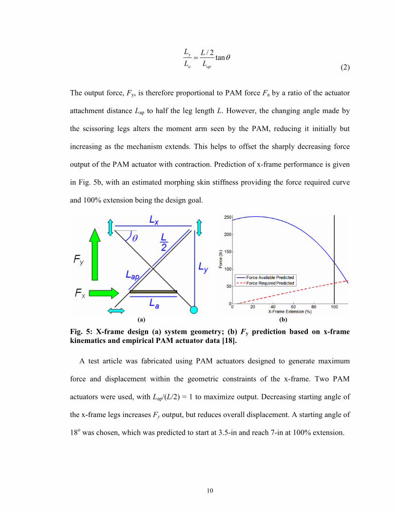
The output force, Fy, is therefore proportional to PAM force Fa by a ratio of the actuator

attachment distance Lap to half the leg length L. However, the changing angle made by

the scissoring legs alters the moment arm seen by the PAM, reducing it initially but

increasing as the mechanism extends. This helps to offset the sharply decreasing force

output of the PAM actuator with contraction. Prediction of x-frame performance is given

in Fig. 5b, with an estimated morphing skin stiffness providing the force required curve

and 100% extension being the design goal.

(a) (b)

Fig. 5: X-frame design (a) system geometry; (b) Fy prediction based on x-frame

kinematics and empirical PAM actuator data [18].

A test article was fabricated using PAM actuators designed to generate maximum

force and displacement within the geometric constraints of the x-frame. Two PAM

actuators were used, with Lap/(L/2) = 1 to maximize output. Decreasing starting angle of

the x-frame legs increases Fy output, but reduces overall displacement. A starting angle of

18o was chosen, which was predicted to start at 3.5-in and reach 7-in at 100% extension.

11

Testing was conducted on an MTS machine as shown in Fig. 6, where force versus

displacement was characterized with the actuator pressure held constant at 90 psi gauge.

Active length Ly was defined as the distance between the pinned ends of the x-frame legs

as in Fig. 5a, with zero displacement defined at the starting 18° leg angle. The x-frame

mechanism was allowed to extend from zero displacement until the measured force

output went to zero and then returned to the start position. Force and displacement were

recorded for several cycles and averaged.

(a) (b)

Fig. 6: X-frame testing (a) blocked force; (b) full extension [18].

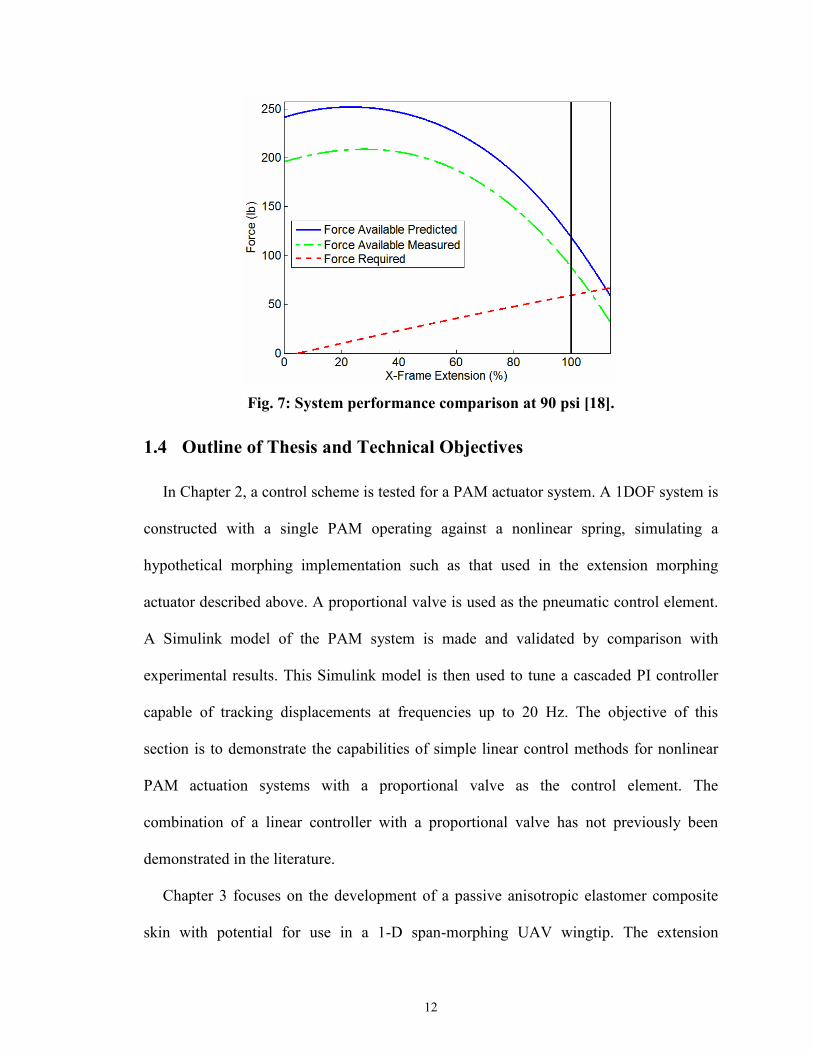
Results of the MTS testing are provided in Fig. 7 as a dash-dotted green line. The

force output prediction, shown as a solid blue line, is based on PAM performance data at

90 psi and x-frame kinematics from Eqns. (1) and (2). Qualitatively, performance

predictions matched the experimental results quite well. A decrease in available force is

seen due to losses in the mechanism, but sufficient excess force was provided in the

design stage that even with losses, the test article is able to exceed the 100% extension

goal for the design skin stiffness.

12

Fig. 7: System performance comparison at 90 psi [18].

1.4 Outline of Thesis and Technical Objectives

In Chapter 2, a control scheme is tested for a PAM actuator system. A 1DOF system is

constructed with a single PAM operating against a nonlinear spring, simulating a

hypothetical morphing implementation such as that used in the extension morphing

actuator described above. A proportional valve is used as the pneumatic control element.

A Simulink model of the PAM system is made and validated by comparison with

experimental results. This Simulink model is then used to tune a cascaded PI controller

capable of tracking displacements at frequencies up to 20 Hz. The objective of this

section is to demonstrate the capabilities of simple linear control methods for nonlinear

PAM actuation systems with a proportional valve as the control element. The

combination of a linear controller with a proportional valve has not previously been

demonstrated in the literature.

Chapter 3 focuses on the development of a passive anisotropic elastomer composite

skin with potential for use in a 1-D span-morphing UAV wingtip. The extension

13

morphing actuator described above is mated to an elastomeric skin with anisotropic fiber

reinforcement and a bonded high strain honeycomb substructure. The skin is capable of

sustaining 100% active strain with negligible major axis Poisson effects, giving a 100%

change in surface area, and can withstand typical aerodynamic loads, assumed to range

up to 200 psf (9.58 kPa) for a maneuvering flight surface, with minimal out-of-plane

deflection. The objective of this section is to advance the state of the art of elastomeric

morphing skins by designing a skin specifically for a variable span wing using

reinforcement techniques not seen before in the literature for this application.

Chapter 4 contains the conclusions of the thesis and provides suggestions for future

work.

14

Chapter 2 Pneumatic Actuator System Modeling and Control

2.1 Overview

In order to implement a morphing skin powered by a PAM actuator, the shortcomings

in the control of PAM systems needed to be addressed. A PAM morphing system would

need to track inputs up to at least 5 Hz for flight control, while inputs up to 20-30 Hz or

more are desired for higher order control. To achieve this, a separate test stand, the Single

PAM Test Apparatus (SPTA) was constructed to characterize the performance of a single

PAM under simulated operating conditions. Detailed attention was paid to the design of

the pneumatic system providing air to the actuator as the capabilities of the pneumatics

determined the performance limits and controllability of the PAM to a great degree. A

detailed model of the SPTA was then developed in Simulink to capture the behavior of

the PAM system up to 35 Hz and validated by comparison with experimental results.

Finally, linear controllers were compared using the Simulink model, and a PID controller

was selected for experimental testing. Control gains were chosen using Zeigler-Nichols

tuning with acceptable results over a range of frequencies, demonstrating the

effectiveness of linear control on PAM actuation systems.

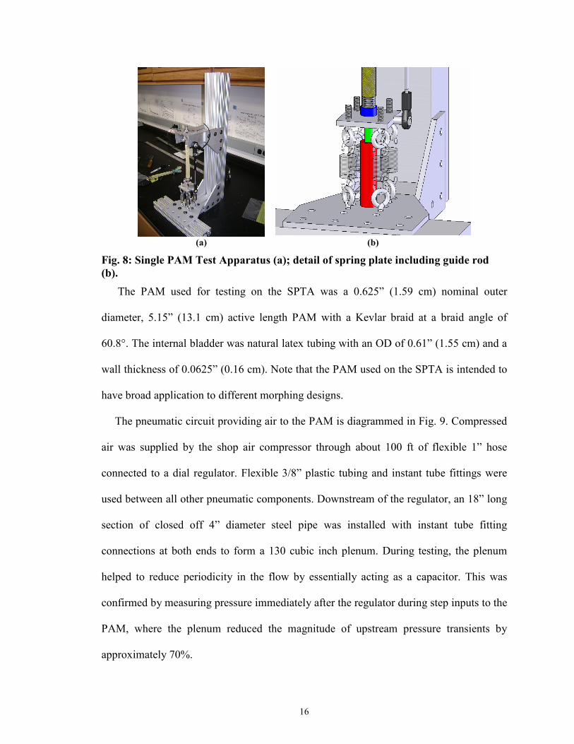
2.2 SPTA Description

The Single PAM Test Apparatus attempted to emulate the operation of a PAM

actuator straining a morphing skin in a nonlinear arrangement such as the scissoring

frame developed in the previous chapter, but in a generalized fashion. The apparatus,

15

shown in Fig. 8a, consists primarily of a frame with a cantilevered C-channel aluminum

beam attached in an adjustable manner to a vertical 80/20 aluminum post fixed to an

80/20 base. This frame was clamped to a lab table during testing to prevent movement.

The PAM actuator is secured at the top to the cantilevered beam by a threaded rod which

has an air-through hole to provide pressurized air to the PAM. An Omegadyne PX209-

200G5V pressure transducer measures the PAM pressure via an aluminum block which

was screws directly onto the threaded air-through rod. The bottom of the PAM is attached

to a flat plate shown in Fig. 8b by means of the threaded ends of a Honeywell Sensotech

Model 31 1000lb load cell in line with the PAM. To one edge of the plate is bolted the

moving end of an Omega LP804-2 LVDT position sensor, the fixed end of which is

attached to the cantilevered beam. This sensor measures the motion of the spring plate as

the PAM contracts, with contraction regarded as positive by convention.

The plate has eye hooks for four springs arranged in parallel and sized to provide

approximately 3% strain in the test PAM at 90 psi (621 kPa). The springs are not loaded

beyond their initial steeper spring rate, leading to a two-part piecewise nonlinear spring

rate which stands in for the nonlinearity of an actual morphing load. The springs are fixed

via four similar eyehooks to the base of the frame. To constrain the system to motion in

the vertical axis, a hollow aluminum guide tube was attached to the base between the four

springs. A steel rod fixed to the bottom of the spring plate slides in sleeve bearings which

line the guide tube, preventing side to side motion of the PAM during operation. Detail of

the spring plate/guide rod arrangement is shown in Fig. 8b.

16

(a) (b)

Fig. 8: Single PAM Test Apparatus (a); detail of spring plate including guide rod

(b).

The PAM used for testing on the SPTA was a 0.625” (1.59 cm) nominal outer

diameter, 5.15” (13.1 cm) active length PAM with a Kevlar braid at a braid angle of

60.8°. The internal bladder was natural latex tubing with an OD of 0.61” (1.55 cm) and a

wall thickness of 0.0625” (0.16 cm). Note that the PAM used on the SPTA is intended to

have broad application to different morphing designs.

The pneumatic circuit providing air to the PAM is diagrammed in Fig. 9. Compressed

air was supplied by the shop air compressor through about 100 ft of flexible 1” hose

connected to a dial regulator. Flexible 3/8” plastic tubing and instant tube fittings were

used between all other pneumatic components. Downstream of the regulator, an 18” long

section of closed off 4” diameter steel pipe was installed with instant tube fitting

connections at both ends to form a 130 cubic inch plenum. During testing, the plenum

helped to reduce periodicity in the flow by essentially acting as a capacitor. This was

confirmed by measuring pressure immediately after the regulator during step inputs to the

PAM, where the plenum reduced the magnitude of upstream pressure transients by

approximately 70%.

17

Fig. 9: Pneumatic circuit setup; distances between components less than 3” unless

noted.

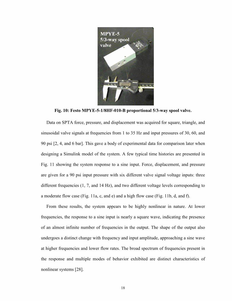
Flow control was provided by a Festo MPYE-5-1/8HF-010-B, a proportional 5/3-way

spool valve. The valve consists of a sliding spool that alternately connects two output

ports to either a pressure source or an exhaust port. This allows two actuators to be

controlled simultaneously in a bi-directional manner. In this study a single actuator was

operated while the second output port was blocked off. The spool position is varied

continuously via a solenoid coil. The coil is powered by a 17-30 V excitation and

controlled by an analog input signal of 0-10 V. By applying a signal voltage to change

the spool position, valve orifice cross-sectional area can be continuously varied, giving

control over flow rate to the PAM. The spool valve has a fast response time of 5 ms, and

an operating pressure range from 0-10 bar, delivering 700 l/min at a nominal pressure of

6 bar.

18

Fig. 10: Festo MPYE-5-1/8HF-010-B proportional 5/3-way spool valve.

Data on SPTA force, pressure, and displacement was acquired for square, triangle, and

sinusoidal valve signals at frequencies from 1 to 35 Hz and input pressures of 30, 60, and

90 psi [2, 4, and 6 bar]. This gave a body of experimental data for comparison later when

designing a Simulink model of the system. A few typical time histories are presented in

Fig. 11 showing the system response to a sine input. Force, displacement, and pressure

are given for a 90 psi input pressure with six different valve signal voltage inputs: three

different frequencies (1, 7, and 14 Hz), and two different voltage levels corresponding to

a moderate flow case (Fig. 11a, c, and e) and a high flow case (Fig. 11b, d, and f).

From these results, the system appears to be highly nonlinear in nature. At lower

frequencies, the response to a sine input is nearly a square wave, indicating the presence

of an almost infinite number of frequencies in the output. The shape of the output also

undergoes a distinct change with frequency and input amplitude, approaching a sine wave

at higher frequencies and lower flow rates. The broad spectrum of frequencies present in

the response and multiple modes of behavior exhibited are distinct characteristics of

nonlinear systems [28].

19

1 2 3 4 50

100

200Sine Input, 1Hz, 3.3V to 6.3V

Force, lb

1 2 3 4 5

-0.1

0

0.1

Displacement, in

1 2 3 4 50

50

100

Pressure, psi

Time, s

1 2 3 4 50

100


Force, lb

1 2 3 4 5

-0.1

0

0.1

Displacement, in

1 2 3 4 50

50

100

Pressure, psi

Time, s

(a) (b)

0.2 0.3 0.4 0.5 0.6 0.70

100


Force, lb

0.2 0.3 0.4 0.5 0.6 0.7

-0.1

0

0.1

Displacement, in

0.2 0.3 0.4 0.5 0.6 0.70

50

100

Pressure, psi

Time, s

0.2 0.3 0.4 0.5 0.6 0.70

100


Force, lb

0.2 0.3 0.4 0.5 0.6 0.7

-0.1

0

0.1Displacement, in

0.2 0.3 0.4 0.5 0.6 0.70

50

100

Pressure, psi

Time, s

(c) (d)

0.1 0.15 0.2 0.25 0.3 0.350

100


Force, lb

0.1 0.15 0.2 0.25 0.3 0.35

-0.1

0

0.1

Displacement, in

0.1 0.15 0.2 0.25 0.3 0.350

50

100

Pressure, psi

Time, s

0.1 0.15 0.2 0.25 0.3 0.350

100


Force, lb

0.1 0.15 0.2 0.25 0.3 0.35

-0.1

0

0.1

Displacement, in

0.1 0.15 0.2 0.25 0.3 0.350

50

100

Pressure, psi

Time, s

(e) (f)

Fig. 11: SPTA force, displacement, and pressure for sine inputs at 1, 7, and 14 Hz

and three voltage inputs: moderate flow (a, c, and e) and higher flow (b, d, and f).

20

2.3 SPTA Model Development and Verification

The first step to developing a controller for the SPTA was to construct a mathematical

model of the physical system. Each individual component was described analytically or

empirically and incorporated into the model. The model was then implemented in

Simulink and validated by comparison with experimental data. The main components of

the SPTA model were the mechanical system dynamics, the mass flow through the valve

and connecting tubing, the pressure change in the PAM as a result of mass flow, and the

force output of the PAM itself based upon pressure and displacement. The equation of

motion governing the SPTA dynamics is given by:

f s pMx F F F W+ + = −��

(3)

where M and W are the mass and weight of the moving parts of the system (spring plate,

eye hooks, load cell, position sensor attachment bolt), x is the PAM position, Fp is the

PAM force, and Fs is the spring force. The friction force on the guide rod under the

spring plate, Ff, was incorporated into a general viscous friction force discussed later.

Fig. 12: Free body diagram of spring plate assembly.

21

2.3.1 PAM Force Model

A review of methods for prediction of PAM force output reveals a number of different

models, all of which suffer from large errors or require empirical actuator

characterization for accuracy. Most are based on an energy conservation approach, with

each model having a similar combination of geometric and experimentally determined

parameters relating force to pressure and displacement [25]. In one model for a PAM

system controller, Caldwell et al. suggest calculating PAM force based on the driving

force generated due to volume change away from the lowest energy state due to braid

reorientation at different PAM displacements [19]. This method produces the correct

qualitative response but is different from the actual PAM force by up to 50% due to the

non-ideal losses. A similar initial approach was taken by Hildebrandt et al. [29] who

subsequently modeled the PAM as a pneumatic cylinder with an empirically determined

“virtual piston area” to account for non-ideal losses. Another model by van der Linde

[30] uses a lumped parameter model that relies on work by Chou and Hannaford [31] for

PAM force, with a number of parameters estimated empirically. The model also assumes

constant PAM volume, which is not a valid assumption for the larger displacements seen

in the research presented here. Kothera et al. [21] improve upon an older model by

Gaylord [32] with the addition of a number of further parameters to account for non-

cylindrical bladder shape and the nonlinear stiffness when stretched. However, this model

still exhibits some error and requires parameter estimation from experiment.

The purpose of this research was control of a morphing control surface and not

refinement of PAM actuator models. Thus it was decided to rely on lookup tables based

on empirical actuator data, rather than a predictive model, to provide the PAM force term

22

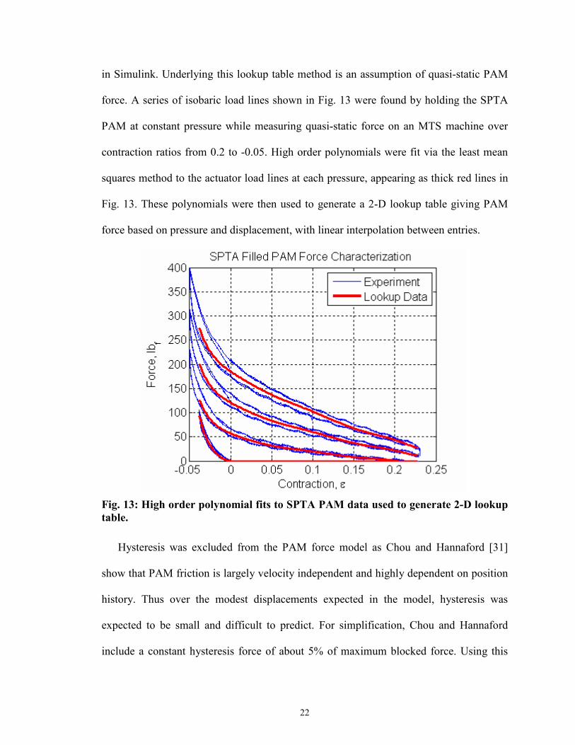
in Simulink. Underlying this lookup table method is an assumption of quasi-static PAM

force. A series of isobaric load lines shown in Fig. 13 were found by holding the SPTA

PAM at constant pressure while measuring quasi-static force on an MTS machine over

contraction ratios from 0.2 to -0.05. High order polynomials were fit via the least mean

squares method to the actuator load lines at each pressure, appearing as thick red lines in

Fig. 13. These polynomials were then used to generate a 2-D lookup table giving PAM

force based on pressure and displacement, with linear interpolation between entries.

Fig. 13: High order polynomial fits to SPTA PAM data used to generate 2-D lookup

table.

Hysteresis was excluded from the PAM force model as Chou and Hannaford [31]

show that PAM friction is largely velocity independent and highly dependent on position

history. Thus over the modest displacements expected in the model, hysteresis was

expected to be small and difficult to predict. For simplification, Chou and Hannaford

include a constant hysteresis force of about 5% of maximum blocked force. Using this

23

approach in the Simulink model was found to negatively affect system stability and

simulation results. Instead, a small viscous damping force was introduced to account for

friction throughout the system, resulting in a better match with experimental data.

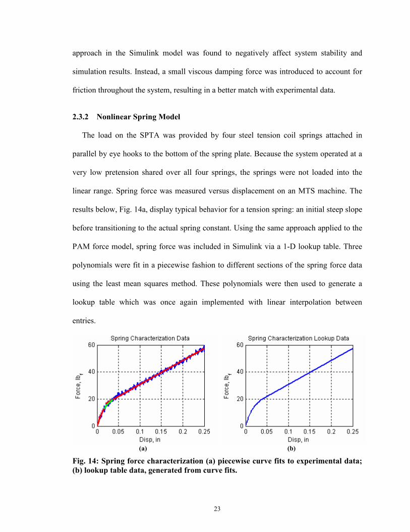
2.3.2 Nonlinear Spring Model

The load on the SPTA was provided by four steel tension coil springs attached in

parallel by eye hooks to the bottom of the spring plate. Because the system operated at a

very low pretension shared over all four springs, the springs were not loaded into the

linear range. Spring force was measured versus displacement on an MTS machine. The

results below, Fig. 14a, display typical behavior for a tension spring: an initial steep slope

before transitioning to the actual spring constant. Using the same approach applied to the

PAM force model, spring force was included in Simulink via a 1-D lookup table. Three

polynomials were fit in a piecewise fashion to different sections of the spring force data

using the least mean squares method. These polynomials were then used to generate a

lookup table which was once again implemented with linear interpolation between

entries.

(a) (b)

Fig. 14: Spring force characterization (a) piecewise curve fits to experimental data;

(b) lookup table data, generated from curve fits.

24

2.3.3 PAM Pressure Model

To use the PAM force data described above, an accurate model is needed to determine

internal pressure based on mass flow into the PAM. Richer and Hurmuzlu [33] derive an

expression for pressure change in a container of changing volume using the ideal gas law,

conservation of mass, and conservation of energy:

( ) in in out out

RT VP m m P

V Vα α α= − −

��

(4)

Here R is the gas constant for the medium, T is the upstream temperature, V is the

actuator volume, and the α coefficients are specific heat ratios for the different processes.

According to work by Al-Ibrahim and Otis [34] on pneumatic cylinders as related by

Richer and Hurmuzlu, the pressure change is approximately adiabatic only during inflow,

where the specific heat coefficient can be estimated as αin = 1.4. During exhaust the

process was nearly isothermal and the specific heat αout = 1 is appropriate. For pressure

change due to changing volume the process is somewhere between adiabatic and

isothermal and the specific heat can be approximated as α = 1.2.

Unlike a pneumatic cylinder, the internal volume of a PAM is difficult to determine

during operation. While a pneumatic cylinder’s volume can be calculated based upon its

geometry and cylinder position, the bladder and braid of a PAM will change shape

nonlinearly when inflated. For a PAM with a very stiff braid material, the geometry of

the braid will limit the expansion of the bladder and should lead to a volume change

which is not dependent on pressure. As the braid angle changes, the PAM expands

radially and contracts axially, leading to a nonlinear relationship between displacement

and volume when pressurized.

25

To measure this relationship, a volume measurement device was attached to the MTS

machine used to characterize PAMs. The device, shown in Fig. 15, consists of a water-

filled tube surrounding the PAM, with an observation tube connected by a flexible hose

to the side of the main tube. The water level in the observation tube is measured by a

laser position sensor. The PAM is then pressurized and quasi-static change in water

height is recorded versus contraction ratio. Based upon the cross section of the two tubes,

the change in volume from rest can be determined. The braid and rubber bladder are

essentially incompressible and occupy constant volume during testing. The resting

volume of the PAM bladder, calculated based on geometry, is then added to the change in

volume to yield the total internal volume versus pressure and displacement.

(a) (b)

Fig. 15: PAM volume measurement device (a) design; (b) fabricated assembly.

Results from volume characterization of the SPTA PAM are plotted below in Fig. 15.

Each curve is a high order polynomial fit via the linear least squares method to a curve of

constant pressure. Except below about 10 psi where the PAM does not seem to inflate to

its full shape, the internal volume is largely dictated by braid geometry at a given

26

displacement. There is a slight dependence on pressure above 10 psi, which suggests that

rubber stiffness, friction between braid and rubber or within the braid itself, or even strain

in the braid help dictate the volume that can be achieved for a given pressure. The

polynomials plotted in Fig. 15 were used to generate data points for a 2-D lookup table.

-0.02 0 0.02 0.04 0.06 0.080.2

0.4

0.6

0.8

1

1.2

1.4SPTA Filled PAM Volume Lookup Data

Contraction (ε)

Volume (cu in)

10 psi

0 psi

5 psi

20-90psi

Fig. 16: Volume measurement device for SPTA PAM showing six different

pressures.

2.3.4 Mass Flow through Valve Orifice

Accurately predicting mass flow is both important and difficult for a pneumatic

system. The effects of compressibility and losses throughout the system will affect

performance and should be included in a pneumatic mass flow model. The following

equation predicts steady mass flow through a well-rounded orifice [35], but has also been

found useful for dynamic flow [36]:

1

2

2 /( ) for /

2 /( ) for /

d u d u cr

d u d u cr

A C P C R T P P Pm

A C P C R T P P P

⋅ ⋅ ⋅ ⋅ >=

⋅ ⋅ ⋅ ⋅ ≤�

(5)

27

Here, A is the valve orifice area, Pu and Pd are the absolute pressures upstream and

downstream of the valve, R is the gas constant for the medium, and T is the temperature

upstream of the valve (taken to be room temperature). The terms C1 and C2 are pressure

and medium dependent flow terms for subsonic and sonic flow respectively:

( ) ( )

( )

2/ ( 1) /

1

1/( 1)

2

/( 1) / /

2 /( 1) /( 1)

d u d uC P P P P

C

γ γ γ

γ

γ γ

γ γ γ

+

−

= − −

= + + (6)

The term Cd is a discharge coefficient, capturing losses in the orifice, which is considered

independent of valve position or signal voltage. Pugi et al. [37] give an expression which

approximates Cd for compressible flow based on the ratio of downstream to upstream

pressure:

( ) ( ) ( )

( ) ( )

2 3

4 5

0.8414 0.1001 / 0.8415 / 3.9 / ...

... 4.001 / 1.6827 /

d d u d u d u

d u d u

C P P P P P P

P P P P

= − + −

+ − (7)

With this, all terms required to find mass flow can be calculated except for valve cross

sectional area, which must be found through valve characterization. Losses due to

neglecting tubing should also be included in a mass flow model and will be discussed

later.

2.3.5 Valve Area Characterization

In order to use the Festo MPYE 5/3-way proportional valve to control PAM position,

the cross sectional area of the valve orifice must be quantified as a function of input

voltage. Based on knowledge of mass flow rate, Eq. (5) can be solved for valve orifice

area. To experimentally measure dynamic mass flow rate, the valve was used to fill and

28

exhaust a fixed volume container. Flow rate was then estimated based upon the pressure

history and used to characterize valve area versus voltage. The small steel pressure vessel

shown in Fig. 17 was constructed for this purpose, with a volume of approximately 15 cu.

in., an input port on one end, and a pressure transducer on the other.

Fig. 17: Steel pressure vessel for spool valve characterization.

(a) (b) (c)

Fig. 18: 5/3-way spool valve operation (a) port 2 open to source; (b) neutral; (c) port

4 open to source.

The Festo MPYE 5/3-way proportional valve has five ports numbered 1-5 as shown in

Fig. 18 with a sliding spool in the center determining which ports are connected. At an

input signal of 4.8 V, the valve spool is centered such that nominally no flow occurs

(although there is slight leakage), and between 4.3 and 5.3 V there is a deadband region

with very low leakage flow. At voltages lower than 4.3 V, port 2 is connected to the

29

source pressure and port 4 is open to atmosphere, while at voltages above 5.3 V port 4 is

open to source pressure while port 2 is connected to atmosphere. Flow rate for both

inflow and exhaust is related to the difference of the signal voltage from the neutral

voltage.

A series of tests were conducted to characterize the inflow and exhaust flow rates for

each of the two output ports using a 90 psi source pressure. The pressure vessel was

connected to one of two output ports, either port 2 or port 4, by a very short length of

3/8” tubing so that the impact of connecting tubing losses on flow rate could be

neglected. The unused output port was blocked during characterization. To measure

inflow into the vessel, the valve was cycled at a low frequency between the fully opened

exhaust voltage and a range of inflow signal voltages from 0 V to 4.8 V for port 2 and 4.8

V to 10 V for port 4. A similar series of tests was run to acquire exhaust data. The valve

was cycled between fully open to input pressure and a range of exhaust signal voltages,

going from 4.8 V to 10 V for port 2 and 0 V to 4.8 V for port 4. The inflow or exhaust

regions of the pressure histories were used to find the time rate of change pressure, from

which mass flow rate and then valve cross sectional area could be determined.

To determine mass flow rate from pressure history, examine Eq. (5). For /d u crP P P≤ ,

flow is choked, and for a given valve area mass flow is linear with upstream pressure Pu.

Theoretically for air the critical downstream/upstream pressure ratio is 0.528. However,

the critical pressure ratio for a specific valve will vary due to geometry and losses in the

valve. Proportional valves can have critical pressure ratios as low as 0 [35], with data for

one model ranging between 0.3 and 0.5 [38]. Due to the difficulty of measuring the

critical pressure ratio, a value of 0.3 was chosen for normal inflow and exhaust and 0.1

30

was chosen for the deadband “leak flow” region based on visual approximation from the

data. By considering only choked flow, the mass flow equation is simplified to:

d 2 2 /( ) um A C C RT P= ⋅ ⋅ ⋅�

(8)

This expression for mass flow can be substituted into the pressure change Eq. (4) and

simplified for a fixed volume cylinder:

d 2 2 /( ) u

RTP A C C RT P

Vα= ⋅ ⋅ ⋅ ⋅�

(9)

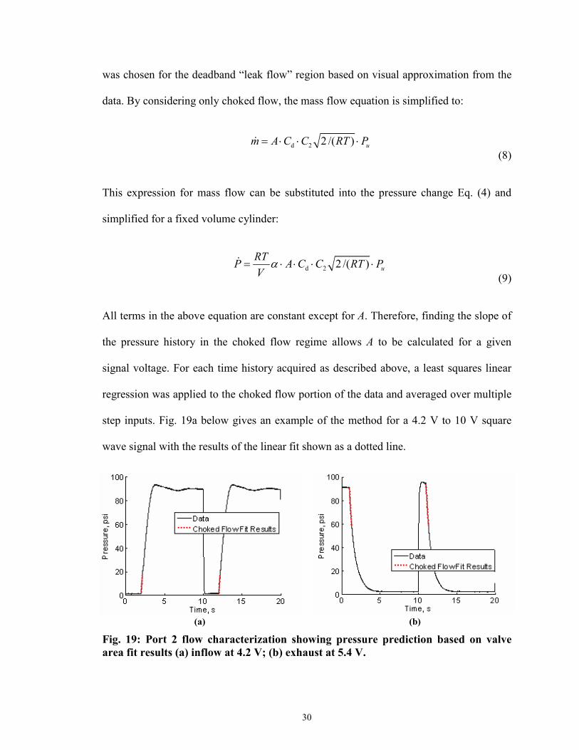
All terms in the above equation are constant except for A. Therefore, finding the slope of

the pressure history in the choked flow regime allows A to be calculated for a given

signal voltage. For each time history acquired as described above, a least squares linear

regression was applied to the choked flow portion of the data and averaged over multiple

step inputs. Fig. 19a below gives an example of the method for a 4.2 V to 10 V square

wave signal with the results of the linear fit shown as a dotted line.

(a) (b)

Fig. 19: Port 2 flow characterization showing pressure prediction based on valve

area fit results (a) inflow at 4.2 V; (b) exhaust at 5.4 V.

31

Exhaust occurs through a separate channel in the valve from inflow and thus requires

separate characterization. A similar method can be followed to find the exhaust area, but

now the upstream pressure, i.e. pressure in the chamber, is no longer constant. An

expression is needed for upstream pressure versus time. Taking the Laplace transform of

Eq. (9) and rearranging, with α = 1 for exhaust flow, yields:

d 2

(0)( )

2 /( )

uu

PP s

RTs A C C RT

V

=+ ⋅ ⋅ (10)

The inverse Laplace yields an expression for upstream pressure as a function of time:

d 2 2/( )

( ) (0)RT

A C C RT tV

u uP t P e⋅ ⋅ ⋅

= ⋅ (11)

This expression can be used to solve for A based on experimental data. Rearranging, a

linear least squares fit for A can be found:

( ) ( )1

d 2/ 2 /( ) log / (0)u uRT V C C RT P P A t−

⋅ ⋅ = ⋅ (12)

By applying the above equation to the pressure data in the choked flow region, it is

possible to find a value for valve area for exhaust flow. Using this valve area, predictions

from Eq. (11) match the pressure history as demonstrated in Fig. 19b.

By applying the above two methods to inflow and exhaust data, the valve area can be

characterized versus signal voltage for both output ports. Results of this characterization

for both ports are given in Fig. 20. Incorporating the characterization data into the

32

Simulink model was a simple matter of importing the valve area versus signal voltage

data into two 1-D lookup tables, one for each port.

Fig. 20: Festo MPYE 5/3-way spool valve characterization results.

2.3.6 Effects of Connecting Tubing

Two different models were used to include the effects of tubing losses on mass flow

for the connecting tubing between the valve and the cylinder. Richer and Hurmuzlu [33]

model the tubing losses in two parts. By assuming a change in mass flow to propagate as

a wave with no dispersion along a short length of smooth tubing, they find a time delay

and amplitude attenuation. The time delay is determined simply by the length of

connecting tubing Lt divided by the speed of sound c, and is modeled as follows:

0 if /( )

( / ) if /

t

delay

t t

t L cm t

m t L c t L c

<=

− ≥�

� (13)

For the amplitude attenuation due to friction, they multiply the mass flow by the

following expression:

33

exp2

t t

d

R RT L

P cφ

−=

(14)

Here, Rt is the tube resistance, Lt is the length of tubing between valve and actuator, and c

is the speed of sound in the fluid. The pressure Pd is called the “end pressure” in their text

and it is assumed this refers to the pressure at the end of the tubing, the downstream

pressure. To simplify the model, fully laminar flow was assumed to determine the tube

resistance based on Rt = 32µ/Dt2, where µ is the fluid viscosity and Dt is the tubing

internal diameter.

A second model as derived by Incropera and DeWitt [39] based on Poiseuille flow

gives the pressure drop required to sustain steady, fully developed internal flow. As an

approximation, this can be used to determine the pressure drop ∆P over the length of

connecting tubing between the valve and the volume to be filled:

2

2

mt

t

uP f L

D

ρ∆ =

(15)

To make use of this equation, three further pieces of information must be calculated.

First, the air density ρ is approximated by the ideal gas law using ambient air temperature

and the average of upstream and downstream pressure. Second, the mean velocity um is

estimated based on the air density, the mass flow as calculated by an initial guess without

tubing losses, and the cross-sectional area of the tubing. Last, the Moody friction factor f

for laminar flow can be calculated in one of two ways. First, for fully laminar flow [39]:

64

ReDf =

(16)

34

The Reynolds number ReD is based on the mean velocity and the internal diameter of the

tubing. For turbulent flow, one method of approximating the friction factor is given by

[39]:

1/ 4 4

1/5 4

0.316Re for Re 2 10

0.184Re for Re 2 10

D D

D D

f

−

−

≤ ×=

> × (17)

The resulting pressure change from Eq. (15) can then be applied to the upstream or

downstream pressure depending on the flow direction. For flow entering the chamber, the

pressure is seen by the valve as a back pressure, and ∆P is added to the downstream

pressure. For exhaust flow, the pressure drop in the connecting tubing results in a head

loss upstream of the valve, and ∆P is subtracted from the upstream pressure. The new

upstream and downstream pressure is then used to calculate a new mass flow. This must

be iterated until the previous mass flow used to find mean velocity and the new mass

flow based on the updated pressures converge.

2.3.7 Pneumatic Model in Simulink

To test the mass flow model and compare the two methods of calculating tubing

losses, a Simulink model was made to simulate the filling and exhausting of a fixed

volume pressure vessel identical to the one used while characterizing the Festo spool

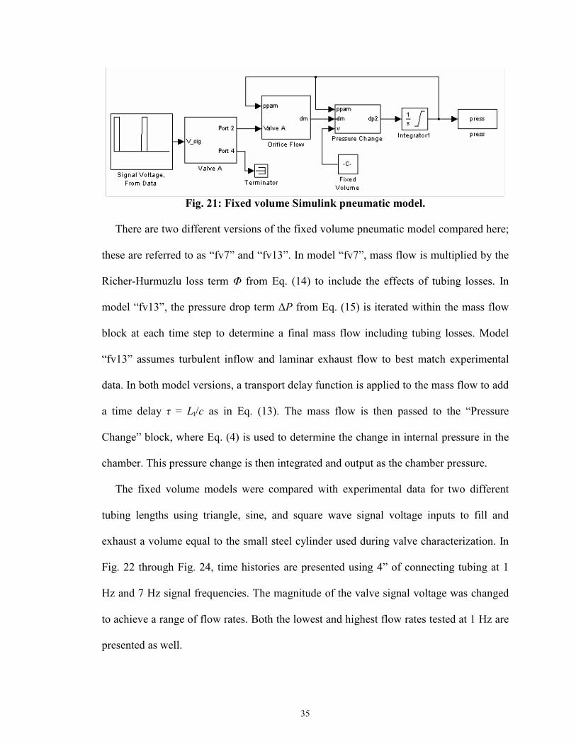
valve. The block diagram of the fixed volume pneumatic model is shown in Fig. 21. A

signal voltage is used to determine spool valve area from the Fig. 20 lookup table data in

the block labeled “Valve A”. The valve area is then passed to the “Orifice Flow” block

containing Eq. (5), where the valve area and current PAM pressure are used to calculate

mass flow through the valve.

35

Fig. 21: Fixed volume Simulink pneumatic model.

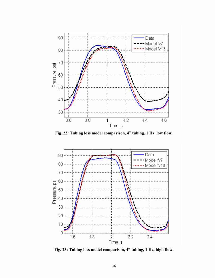
There are two different versions of the fixed volume pneumatic model compared here;

these are referred to as “fv7” and “fv13”. In model “fv7”, mass flow is multiplied by the

Richer-Hurmuzlu loss term Φ from Eq. (14) to include the effects of tubing losses. In

model “fv13”, the pressure drop term ∆P from Eq. (15) is iterated within the mass flow

block at each time step to determine a final mass flow including tubing losses. Model

“fv13” assumes turbulent inflow and laminar exhaust flow to best match experimental

data. In both model versions, a transport delay function is applied to the mass flow to add

a time delay τ = Lt/c as in Eq. (13). The mass flow is then passed to the “Pressure

Change” block, where Eq. (4) is used to determine the change in internal pressure in the

chamber. This pressure change is then integrated and output as the chamber pressure.

The fixed volume models were compared with experimental data for two different

tubing lengths using triangle, sine, and square wave signal voltage inputs to fill and

exhaust a volume equal to the small steel cylinder used during valve characterization. In

Fig. 22 through Fig. 24, time histories are presented using 4” of connecting tubing at 1

Hz and 7 Hz signal frequencies. The magnitude of the valve signal voltage was changed

to achieve a range of flow rates. Both the lowest and highest flow rates tested at 1 Hz are

presented as well.

36

Fig. 22: Tubing loss model comparison, 4” tubing, 1 Hz, low flow.

Fig. 23: Tubing loss model comparison, 4” tubing, 1 Hz, high flow.

37


The models both match the data best at higher flow rates and lower frequencies as

seen in Fig. 23, but still exhibit less than about 10% error at low flow rates and/or high

frequencies as in Fig. 22 and Fig. 24. In general, neither model appears significantly

better at matching experimental data. This result is expected since the tubing loss has

little impact when tubing length is short. As a result they both exhibit small discrepancies

in flow rate which appear as different rates of pressure change during inflow and exhaust.

Next both models are compared using data taken with 24” of connecting tubing

between valve and cylinder. In Fig. 25 and Fig. 26, results for 1 Hz at low and high flow

rates are compared, while in Fig. 27, a 7 Hz high flow result is shown. Results vary

wildly between models, with model “fv13” using the ∆P loss term from Eq. (15)

matching the data well under all conditions, and model “fv7” using the Φ loss term from

Eq. (14) filling and exhausting far too slowly.

38

Fig. 25: Tubing loss model comparison, 24” tubing, 1 Hz, low flow.


39


Based on the results of the fixed volume pneumatic model testing, it is clear that the

Richer and Hurmuzlu term for tubing losses as described in their paper and presented in

Eq. (14) inadequately represents measured behavior. The ∆P loss term from Eq. (15) is

based on a well-known hydrodynamic internal flow pressure drop equation and, when

iterated at each time step, appears to give a much better estimate of tubing losses.

2.3.8 Full SPTA Model in Simulink

The pneumatic model, the system dynamics, and the various component

characterizations were incorporated into a Simulink model of the complete SPTA system,

a diagram of which is presented in Fig. 28. As in the pneumatic model, a signal voltage is

used to determine valve orifice area from a lookup table. Based on the valve area and the

system velocity and displacement, the PAM states can be calculated and the PAM output

force, Fp, determined. The system displacement is also used to find spring force, Fs, from

40

a lookup table. From the system dynamics, the forces on the system are summed and new

system velocity and position are determined.

Fig. 28: Full SPTA System Simulink model.

Within the PAM block in Fig. 28, there are two main subroutines: the orifice mass

flow block and the PAM force model itself, shown in Fig. 29. The orifice mass flow

block uses the flow model from “fv13” based on Eqns. (5) and (15), and calculates mass

flow into or out of the PAM based on the valve cross sectional area, supply pressure,

atmospheric pressure, current PAM internal pressure, and connecting tubing properties.

Unlike the fixed volume pneumatic model, the best match to the experimental data

was achieved by assuming turbulent flow for both inflow and exhaust, using Eq. (17) for

the friction factor. Recall that the fixed volume pneumatic model assumed laminar

exhaust flow and achieved good agreement with data. It is possible that during SPTA

testing, the inclusion of a pressure transducer mounting block with a rough internal

surface near the PAM orifice triggers turbulent flow during the exhaust phase, while

during fixed volume testing the pressure transducer was mounted to the rear of the

pressure vessel, where it did not impact the formation of laminar flow exiting the vessel.

41

Fig. 29: PAM block showing orifice flow block and PAM force block.

Subsequently, calculation of the PAM states can be carried out inside the PAM force

block, details of which are shown in Fig. 30. The following sequence of steps is carried

out to determine the PAM internal pressure and ultimately the PAM force. First, based on

the position and current internal pressure, the PAM volume is found from the volume

lookup table. Internal volume of connecting tubing between valve and PAM is added to

find total volume. The total volume, current internal pressure, and mass flow are then

used to find the rate change in internal pressure from Eq. (4), which is integrated to find

the new internal pressure. The system position and new internal pressure are then used to

find the PAM force from a lookup table. A small amount of viscous damping is included

to better match the system experimental behavior.

Fig. 30: PAM Force block, where volume, pressure, and then output force are

found.

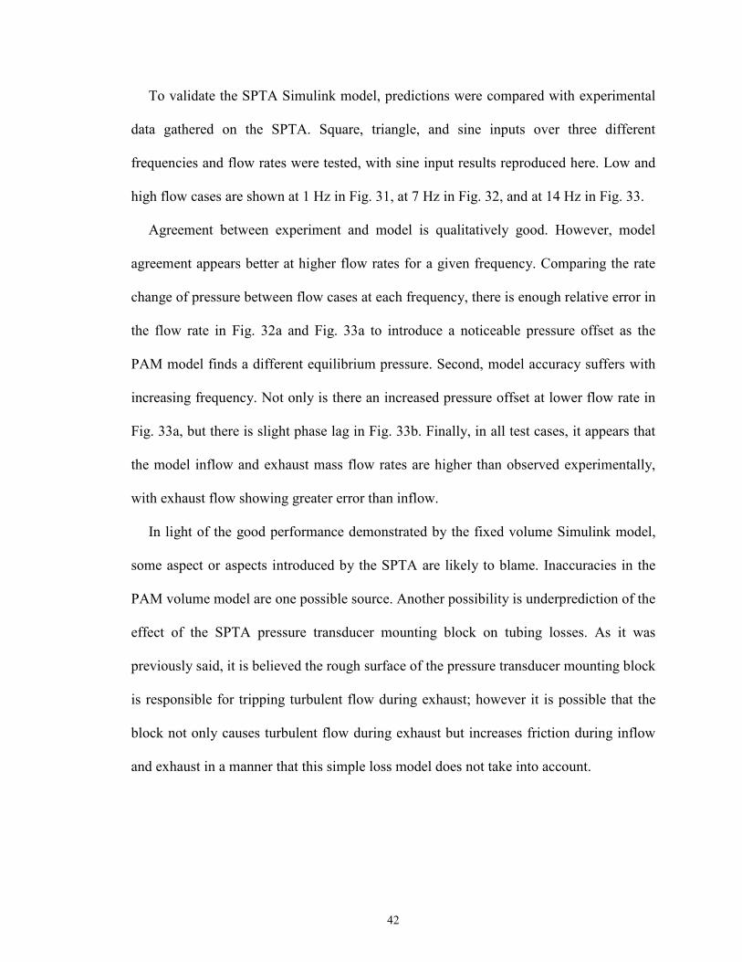
42

To validate the SPTA Simulink model, predictions were compared with experimental

data gathered on the SPTA. Square, triangle, and sine inputs over three different

frequencies and flow rates were tested, with sine input results reproduced here. Low and

high flow cases are shown at 1 Hz in Fig. 31, at 7 Hz in Fig. 32, and at 14 Hz in Fig. 33.

Agreement between experiment and model is qualitatively good. However, model

agreement appears better at higher flow rates for a given frequency. Comparing the rate

change of pressure between flow cases at each frequency, there is enough relative error in

the flow rate in Fig. 32a and Fig. 33a to introduce a noticeable pressure offset as the

PAM model finds a different equilibrium pressure. Second, model accuracy suffers with

increasing frequency. Not only is there an increased pressure offset at lower flow rate in

Fig. 33a, but there is slight phase lag in Fig. 33b. Finally, in all test cases, it appears that

the model inflow and exhaust mass flow rates are higher than observed experimentally,

with exhaust flow showing greater error than inflow.

In light of the good performance demonstrated by the fixed volume Simulink model,

some aspect or aspects introduced by the SPTA are likely to blame. Inaccuracies in the

PAM volume model are one possible source. Another possibility is underprediction of the

effect of the SPTA pressure transducer mounting block on tubing losses. As it was

previously said, it is believed the rough surface of the pressure transducer mounting block

is responsible for tripping turbulent flow during exhaust; however it is possible that the

block not only causes turbulent flow during exhaust but increases friction during inflow

and exhaust in a manner that this simple loss model does not take into account.

43

(a)

(b)

Fig. 31: SPTA model comparison, 1 Hz sine input (a) low flow; (b) high flow.

44

(a)

(b)


45

(a)

(b)


46

2.4 SPTA Controller

The principal objective of this project was to demonstrate the effectiveness of a linear

controller on a PAM actuator. To do so, two different controllers, one PI and one PID,

were implemented in simulation using displacement feedback, and the better of the two

was then tested experimentally on the physical system to verify the simulation results.

2.4.1 SPTA Controller Design

Control was achieved by feeding back PAM displacement and comparing to a

reference displacement, rd, as shown in the Simulink diagram in Fig. 35. The resulting

error was input to a built-in PID control block, whose output ud provided the signal

voltage input for the proportional valve. Because the valve accepted signal voltages from

0-10 V and the controller would output both positive and negative voltages, a bias of 4.8

V was added to ud to provide a neutral signal when no inflation or deflation was

commanded. Control gains for both a PID and a PI controller were calculated based on

Ziegler and Nichols’ tuning rules [40].

Fig. 34: Displacement feedback control diagram.

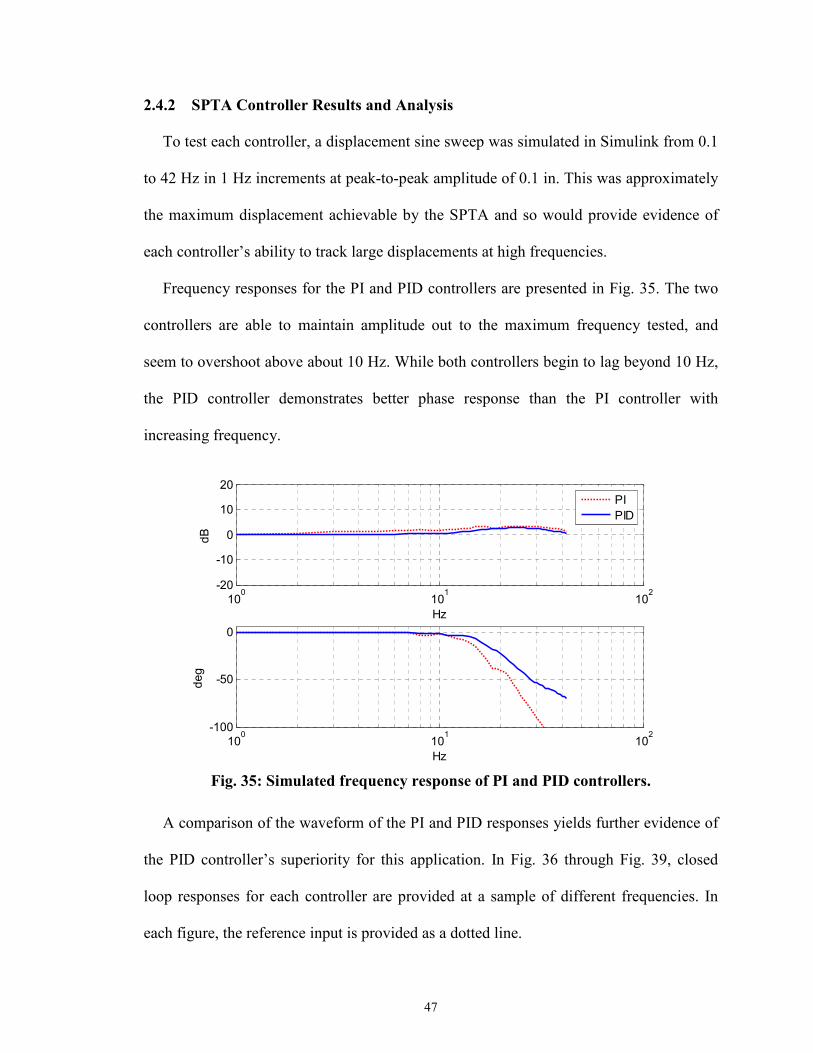
47

2.4.2 SPTA Controller Results and Analysis

To test each controller, a displacement sine sweep was simulated in Simulink from 0.1

to 42 Hz in 1 Hz increments at peak-to-peak amplitude of 0.1 in. This was approximately

the maximum displacement achievable by the SPTA and so would provide evidence of

each controller’s ability to track large displacements at high frequencies.

Frequency responses for the PI and PID controllers are presented in Fig. 35. The two

controllers are able to maintain amplitude out to the maximum frequency tested, and

seem to overshoot above about 10 Hz. While both controllers begin to lag beyond 10 Hz,

the PID controller demonstrates better phase response than the PI controller with

increasing frequency.

100

101

102

-20

-10

0

10

20

Hz

dB

100

101

102

-100

-50

0

Hz

deg

PI

PID

Fig. 35: Simulated frequency response of PI and PID controllers.

A comparison of the waveform of the PI and PID responses yields further evidence of

the PID controller’s superiority for this application. In Fig. 36 through Fig. 39, closed

loop responses for each controller are provided at a sample of different frequencies. In

each figure, the reference input is provided as a dotted line.

48

1 1.5 2 2.5 3 3.5 4 4.5 5

-0.05

0

0.05

PI

Disp., in

Reference

PI Response

1 1.5 2 2.5 3 3.5 4 4.5 5

-0.05

0

0.05PID

Time, s

Disp., in

Reference

PID Response

Fig. 36: SPTA simulation, controller comparison, 0.1” sine input, 1 Hz.

1 1.1 1.2 1.3 1.4 1.5 1.6 1.7 1.8-0.1

-0.05

0

0.05

PI

Disp., in

Reference

PI Response

1 1.1 1.2 1.3 1.4 1.5 1.6 1.7 1.8

-0.05

0

0.05

PID

Time, s

Disp., in

Reference

PID Response


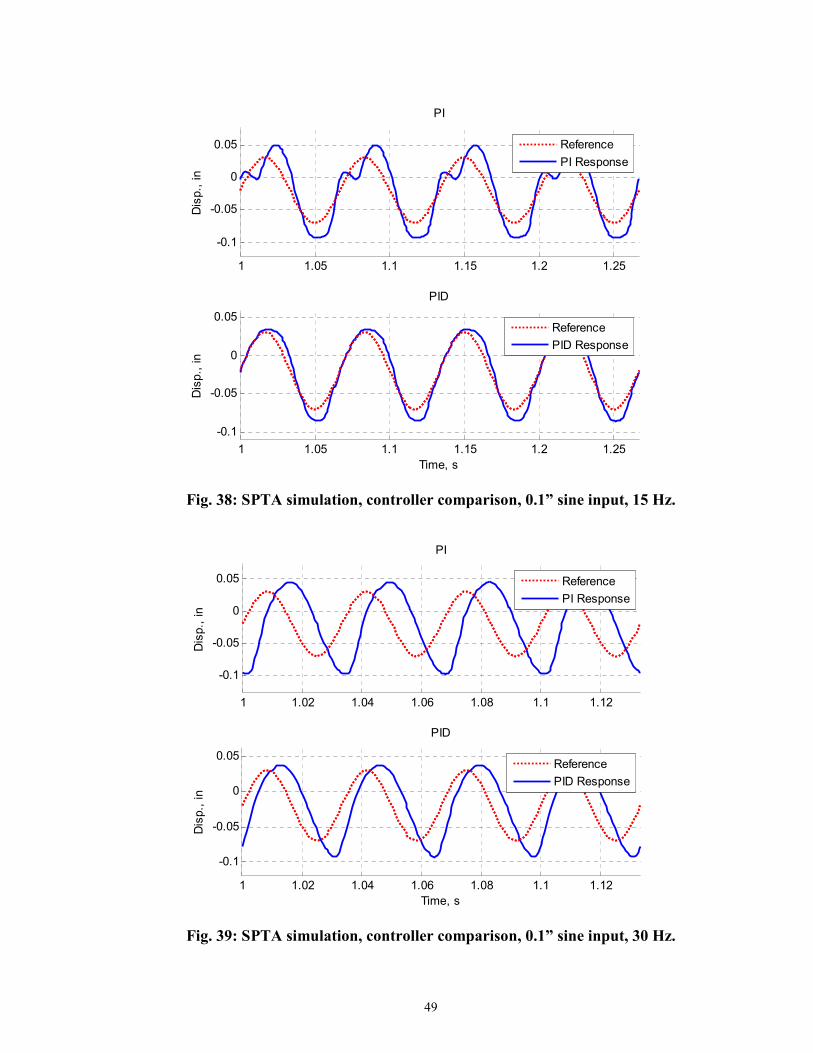
49

1 1.05 1.1 1.15 1.2 1.25

-0.1

-0.05

0

0.05

PI

Disp., in

Reference

PI Response

1 1.05 1.1 1.15 1.2 1.25

-0.1

-0.05

0

0.05

PID

Time, s

Disp., in

Reference

PID Response


1 1.02 1.04 1.06 1.08 1.1 1.12

-0.1

-0.05

0

0.05

PI

Disp., in

Reference

PI Response

1 1.02 1.04 1.06 1.08 1.1 1.12

-0.1

-0.05

0

0.05

PID

Time, s

Disp., in

Reference

PID Response


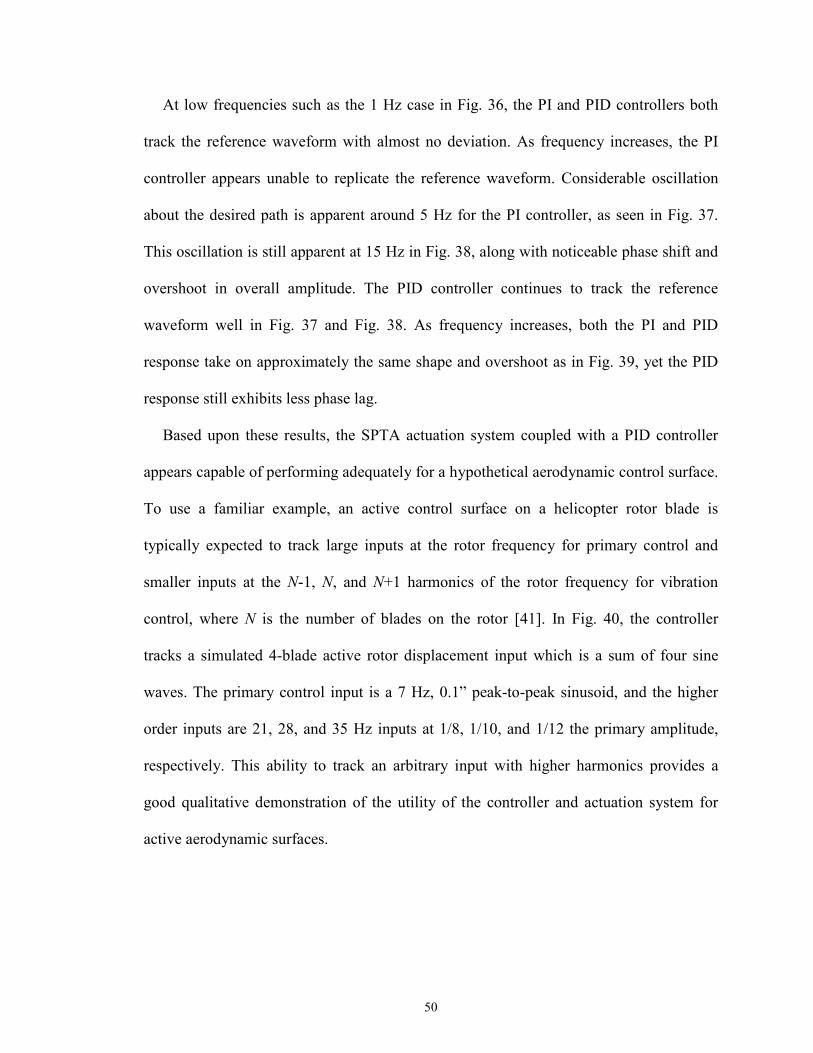
50

At low frequencies such as the 1 Hz case in Fig. 36, the PI and PID controllers both

track the reference waveform with almost no deviation. As frequency increases, the PI

controller appears unable to replicate the reference waveform. Considerable oscillation

about the desired path is apparent around 5 Hz for the PI controller, as seen in Fig. 37.

This oscillation is still apparent at 15 Hz in Fig. 38, along with noticeable phase shift and

overshoot in overall amplitude. The PID controller continues to track the reference

waveform well in Fig. 37 and Fig. 38. As frequency increases, both the PI and PID

response take on approximately the same shape and overshoot as in Fig. 39, yet the PID

response still exhibits less phase lag.

Based upon these results, the SPTA actuation system coupled with a PID controller

appears capable of performing adequately for a hypothetical aerodynamic control surface.

To use a familiar example, an active control surface on a helicopter rotor blade is

typically expected to track large inputs at the rotor frequency for primary control and

smaller inputs at the N-1, N, and N+1 harmonics of the rotor frequency for vibration

control, where N is the number of blades on the rotor [41]. In Fig. 40, the controller

tracks a simulated 4-blade active rotor displacement input which is a sum of four sine

waves. The primary control input is a 7 Hz, 0.1” peak-to-peak sinusoid, and the higher

order inputs are 21, 28, and 35 Hz inputs at 1/8, 1/10, and 1/12 the primary amplitude,

respectively. This ability to track an arbitrary input with higher harmonics provides a

good qualitative demonstration of the utility of the controller and actuation system for

active aerodynamic surfaces.

51

1 1.1 1.2 1.3 1.4 1.5 1.6 1.76080100120140160

Time, s

Force, lbf

1 1.1 1.2 1.3 1.4 1.5 1.6 1.7-0.1

-0.05

0

0.05

Time, s

Displacement, in

Desired

Controlled

1 1.1 1.2 1.3 1.4 1.5 1.6 1.720

40

60

80

Time, s

Pressure, psi

Fig. 40: Prediction of higher order closed loop displacement tracking capability, 7

Hz + 3ω, 4ω, and 5ω sine excitation.

2.5 SPTA Closed Loop Experimental Results

To validate the promising simulation results achieved using PID, a PID controller

implemented in dSPACE was used to control the physical SPTA system. In order to

select the control gains, the values found during simulation by Ziegler-Nichols tuning

were used as a starting point, and optimization was done manually. Gains were

introduced one at a time, proportional, integral, and then derivative, and adjusted by hand

to find an optimum value before the next gain was included. The proportional and

derivative gains from simulation was found to be appropriate, but integral gain was

reduced by a factor of roughly 4, and a 50 Hz low pass Butterworth filter was included to

prevent the derivative gain from causing instability. The closed loop response to a 0.1 in

52

sine wave was then measured at a range of frequencies between 0.1 Hz and 42 Hz,

identical to the frequency sweep performed in simulation.

10-1

100

101

102

-20

0

20

Hz

dB

10-1

100

101

102

-100

-50

0

Hz

deg

Model

Exp

Fig. 41: SPTA closed loop frequency response using PID as compared with model.

Frequency response results are presented in Fig. 41 in comparison with model

predictions. The model controller’s integral gain was reduced to the same value used in

experiment when making these plots. However, the low pass filter used in the experiment

was not included here, the effect of which will be discussed later. Note that the

appearance of phase lag coincided with an increase in amplitude for both the model and

physical system. However, the model predicted a slightly lower corner frequency of

about 4 Hz rather than 7-8 Hz for the physical system. Also, the physical system

displayed a slightly steeper increase in phase lag with frequency than the model predicts.

Still, the model predicts the results of the experimental frequency sweep fairly well.

Closer examination of the waveforms produced by the physical closed loop system

reveals important differences between model and experiment. In Fig. 42 through Fig. 45,

model and experimental results are compared at 1, 5, 12, and 24 Hz.

53

1.5 2 2.5 3 3.5 4 4.5 5-0.1

-0.05

0

0.05

Time, s

Disp, in

Ref.

Mod.

0.5 1 1.5 2 2.5 3 3.5 4-0.1

-0.05

0

0.05

Time, s

Disp, in

Ref.

Exp.

Fig. 42: Model PID (top) vs. experiment PID (bottom), 1 Hz.

1.1 1.2 1.3 1.4 1.5 1.6 1.7 1.8-0.1

-0.05

0

0.05

Time, s

Disp, in

Ref.

Mod.

0.1 0.2 0.3 0.4 0.5 0.6 0.7 0.8-0.1

-0.05

0

0.05

Time, s

Disp, in

Ref.

Exp.


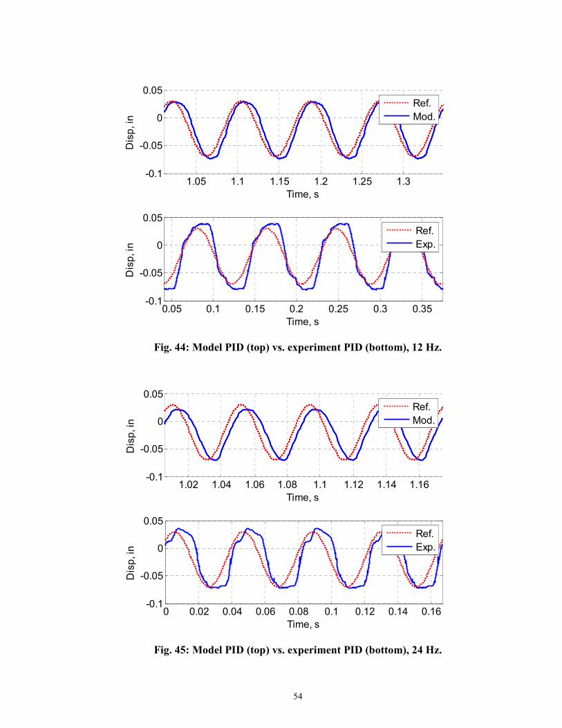
54

1.05 1.1 1.15 1.2 1.25 1.3-0.1

-0.05

0

0.05

Time, s

Disp, in

Ref.

Mod.

0.05 0.1 0.15 0.2 0.25 0.3 0.35-0.1

-0.05

0

0.05

Time, s

Disp, in

Ref.

Exp.


1.02 1.04 1.06 1.08 1.1 1.12 1.14 1.16-0.1

-0.05

0

0.05

Time, s

Disp, in

Ref.

Mod.

0 0.02 0.04 0.06 0.08 0.1 0.12 0.14 0.16-0.1

-0.05

0

0.05

Time, s

Disp, in

Ref.

Exp.


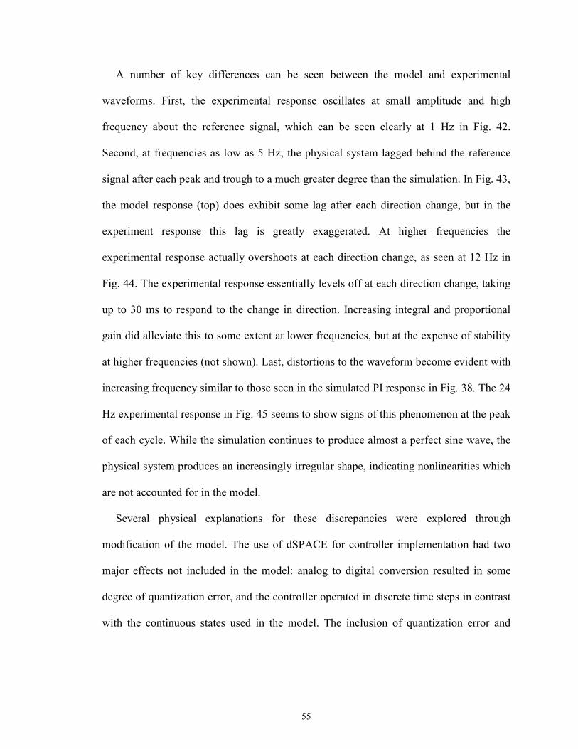
55

A number of key differences can be seen between the model and experimental

waveforms. First, the experimental response oscillates at small amplitude and high

frequency about the reference signal, which can be seen clearly at 1 Hz in Fig. 42.

Second, at frequencies as low as 5 Hz, the physical system lagged behind the reference

signal after each peak and trough to a much greater degree than the simulation. In Fig. 43,

the model response (top) does exhibit some lag after each direction change, but in the

experiment response this lag is greatly exaggerated. At higher frequencies the

experimental response actually overshoots at each direction change, as seen at 12 Hz in

Fig. 44. The experimental response essentially levels off at each direction change, taking

up to 30 ms to respond to the change in direction. Increasing integral and proportional

gain did alleviate this to some extent at lower frequencies, but at the expense of stability

at higher frequencies (not shown). Last, distortions to the waveform become evident with

increasing frequency similar to those seen in the simulated PI response in Fig. 38. The 24

Hz experimental response in Fig. 45 seems to show signs of this phenomenon at the peak

of each cycle. While the simulation continues to produce almost a perfect sine wave, the

physical system produces an increasingly irregular shape, indicating nonlinearities which

are not accounted for in the model.

Several physical explanations for these discrepancies were explored through

modification of the model. The use of dSPACE for controller implementation had two

major effects not included in the model: analog to digital conversion resulted in some

degree of quantization error, and the controller operated in discrete time steps in contrast

with the continuous states used in the model. The inclusion of quantization error and

56

conversion to a fixed time step discrete solution had no discernable effect on the model

results.

As mentioned previously, the low pass Butterworth filter applied to the sensor data in

the experimental implementation of the controller was not included in the model

predictions in Fig. 42 through Fig. 45. Some testing was done to determine the effects of

the filter on the model, but the results were inconsistent in terms of matching the

experiment qualitatively. At low frequencies, the inclusion of the filter seemed to

improve the model’s agreement with experiment, as seen in Fig. 46. The small, high

frequency oscillation about the reference signal displayed by the experiment in Fig. 42

was replicated by inclusion of the filter.

1.48 1.49 1.5 1.51 1.52 1.53 1.54 1.55 1.56 1.57 1.58-0.03

-0.02

-0.01

0

0.01

0.02

Time, s

Disp, in

Reference

w/Filter

0.63 0.64 0.65 0.66 0.67 0.68 0.69 0.7 0.71 0.72

-0.02

-0.01

0

0.01

0.02

0.03

Time, s

Disp, in

Reference

Experiment

Fig. 46: Effect on model of including low pass Butterworth filter at 2 Hz

57

However, at frequencies above about 4 Hz, the model results continued to exhibit

larger and larger oscillations which were not evident in the experimental results. The

divergence was wide enough that the filter effects were not included in the final model

predictions. While the filter definitely has some impact on the system, there must be

further unmodeled nonlinearities contributing to the high frequency content seen in the

experimental results in Fig. 43 through Fig. 45.

Therefore, in spite of their apparently similar frequency responses, the closed loop

SPTA system’s displacement waveform differed from the simulation at higher

frequencies. The helicopter active rotor input simulated in Fig. 40 was repeated in

experiment to illustrate the simulation limitations. The same input was used, a 0.1 in

amplitude 7 Hz sine wave with higher harmonics at 21 Hz, 28 Hz, and 35 Hz included at

lower amplitudes. The closed loop physical response displayed in Fig. 47 largely tracks

the input, but as expected fails to track the higher harmonics as well as simulation would

suggest.

0 0.1 0.2 0.3 0.4 0.5-0.1

-0.08

-0.06

-0.04

-0.02

0

0.02

0.04

Time, s

Disp, in

Measured

Reference

Fig. 47: Experimental closed loop tracking of higher order harmonic input, 7 Hz +

3ω, 4ω, and 5ω sine excitation.

58

Evaluating system performance based on the control requirements for a fixed-wing

UAV, rather than a hypothetical active rotor input, provides a better yardstick for the

SPTA controller’s usefulness. As a starting point, human pilot bandwidth can be as high

as 5-7 Hz, but more realistically is approximately 3 Hz [42,43]. Thus control actuation in

response to pilot inputs appears well within the capabilities of the controller/actuator

simulated here.

For a UAV, however, smaller scale and lighter weight will lead to reduced inertias and

higher natural frequencies than manned craft. Therefore higher bandwidth actuators will

be required for stabilization of modes. Using Froude scaling to ensure commonality of

inertia/gravity and air/gravity force ratios, a UAV would have a higher natural frequency

than a larger aircraft by the square root of the scale factor [44]. As an example, a UAV

four times smaller than a light piloted aircraft would have natural frequencies twice as

high and require twice the actuation bandwidth to stabilize.

Examining the short period mode for a small UAV provides a reasonable minimum

requirement for the SPTA controller’s corner frequency. Assuming the UAV’s short

period frequency can be predicted using Froude scaling, based on a light aircraft with a

wingspan of 36 ft and a marginally stable short period frequency of 10 rad/s, a UAV with

a 3 ft wingspan would have a short period frequency of 34.6 rad/s or 5.5 Hz. The PAM

actuation system presented here demonstrated useful waveform tracking with low phase

lag to roughly 8 Hz. Based upon 5.5 Hz as the desired operating frequency, the PAM

actuation system would be sufficient for control and stabilization of even a small UAV.

59

2.6 Conclusion

A PID displacement feedback controller was designed for a single PAM working

against a spring with nonlinear stiffness. First a physical system was fabricated and

characterized. A Simulink model of the system was then developed and validated using

experimental data. The model was used to compare PI and PID control over a large range

of operating frequencies. The PID controller displayed superior frequency response and

output waveform and was implemented on the physical system to confirm model

predictions.

1. The SPTA Simulink model relied heavily on characterization of certain system

components, particularly the pneumatic valve and the PAM actuator. Unmodeled

nonlinearities limit the usefulness of the model above approximately 10 Hz.

However, below this frequency the model matched the nonlinear system

performance acceptably under a variety of conditions and this modeling approach

would be useful as a design tool for future PAM applications.

2. The tubing loss term in Eq. (14) as presented in [33] by Richer and Hurmuzlu does

not appear to predict realistic tubing losses in this simulation. When using the

Richer and Hurmuzlu term, predicted flow rate is far slower than demonstrated by

experiment for any appreciable tubing length. Assuming Poiseuille flow to calculate

pressure drop due to tubing loss provided a much better prediction of pneumatic

system performance.

3. Displacement feedback PID control of a PAM actuator system using a proportional

valve is shown to be sufficient for tracking a useful range of frequencies at high

displacement. For operation below approximately 8 Hz, the PID controller provides

60

good tracking and waveform replication, results which are sufficient to control a

UAV. This contradicts assertions made in a number of PAM control studies

suggesting an adaptive or nonlinear controller is necessary to stabilize and control a

PAM actuator system at frequencies above 1 Hz. Thus this conclusion makes a

contribution to the literature by testing a combination of proportional valve and

linear PID controller that has not previously been demonstrated on a PAM system

and proving it useful up to 8 Hz.

61

Chapter 3

Design and Fabrication of a Passive 1-D Morphing Aircraft

Skin

3.1 Overview

The primary challenge in developing a morphing skin suitable as an aerodynamic

surface is balancing the competing goals of low in-plane actuation requirements and high

out-of-plane stiffness. In order to make the skin viable, actuation force requirements must

be modest enough to enable a reasonably sized actuation system to stretch the skin to the

desired shape and hold it for the required morphing duration. At the same time, the skin

must support typical aerodynamic loads without deforming excessively (e.g., rippling or

bowing) and degrading the aerodynamic characteristics of the airfoil surface.

a) b) c)

Fig. 48: Overview of morphing skin conceptual design.

To achieve these design goals, a soft, thin silicone elastomer sheet with highly

anisotropic carbon fiber reinforcement called a flexible matrix composite (FMC) would

be oriented such that the fiber-dominated direction runs chordwise at the wingtip, and the

matrix-dominated direction runs spanwise, Fig. 48a. Related research with FMC

62

materials can also be found [45, 46]. Reinforcing carbon fibers controlling the major axis

Poisson’s ratio of the sheet would limit the FMC to 1-D spanwise shape change, Fig. 48b.

For a given bulk stiffness, actuation requirements will increase in proportion to the skin

thickness, ts, while out-of-plane stiffness will be proportional to ts3 by the second moment

of the area. Simply increasing thickness to support out-of-plane loading will therefore

increase in-plane stiffness as well. To meet these competing goals, a flexible modified

honeycomb substructure is desired, Fig. 48c, that is capable of handling out-of-plane

loads without greatly adding to the in-plane stiffness. This allows a thinner skin which, in

turn, reduces actuation requirements. The combined FMC sheet and honeycomb

substructure form a continuous span-morphing skin.

Fig. 49: Proposed morphing skin prototype including PAM actuation system.

63

To motivate the goal of low in-plane stiffness for this research, the skin prototype was

designed in parallel with the span-morphing x-frame actuator mentioned in Chapter 1 and

described in [18]. The PAM driven scissor mechanism is shown in Fig. 49 along with a

mock-up of the proposed morphing skin. Based upon the predicted abilities of the

actuation system, a design skin stiffness was selected that would give greater than 100%

strain capability, as modeled in Fig. 50. In this plot, the dashed curve represents the

maximum available extensile force predicted for the actuation system, and the solid curve

gives the force required to strain the skin based on the design stiffness. Where the two

curves intersect determines the maximum strain capability of the morphing system. A

margin of 15% was added to the design goal to account for anticipated losses due to

friction or manufacturing shortcomings in the skin or actuation system.

Fig. 50: X-frame force predictions and morphing skin stiffness design goal.

In addition, a design goal was selected for out-of-plane deflection requirements. While

under a hypothetical maneuvering wing load of 200 psf (9.58 kPa), an out-of-plane

deflection limit of 0.1 in (2.5 mm) was arbitrarily set. Attempting to keep the skin from

64

deflecting more than this amount gave a reasonable guarantee that the aerodynamic shape

of a large UAV wing morphing structure could be maintained during flight.

3.2 FMC Design and Testing

The primary phase of the morphing skin development was to fabricate the FMC sheet

that would make up the skin or face sheet. A number of design variables were available

for tailoring the FMC to the application, including elastomer stiffness, durometer, ease of

handling during manufacturing, and the quantity, thickness, and angle of carbon fiber

reinforcement.

3.2.1 Elastomer Selection

Initially, a large number of silicone elastomers were tested for viability as matrix

material. Desired properties included maximum elongation well over 100%, a low

stiffness to minimize actuation forces, moderate durometer to avoid having too soft a skin

surface, and good working properties. Workability became a primary challenge to

overcome, as two-part elastomers with high viscosities or very short work times would

not fully wet out the carbon fiber layers. While over a dozen candidate elastomer samples

were examined, only four were selected for further testing. Fig. 51 and Table 1 detail the

silicone elastomers tested as matrix candidates.

65

Fig. 51: Elastomer stress-strain curves.

Table 2: Approximate modulus of elastomers.

Material Modulus (kPa) Modulus (psi)

DC 3-4207 130 19

Sylgard-186 410 59

V-330, CA-45 570 83

V-330, CA-35 330 48

The most promising compositions tested were Dow Corning 3-4207 series and the

Rhodorsil V-330 series. Both exhibited the desired low stiffness and greater than 100%

elongation, but DC 3-4207 suffered from marginal working qualities and lower maximum

elongation and was rejected. Rhodorsil’s V-330 series two-part RTV silicone elastomer

had the right combination of low viscosity and long work time to enable easy and

effective FMC manufacture, and demonstrated high maximum elongation and tear

strength. V-330 CA-35 also had the lowest stiffness of the elastomers tested, excluding

DC 3-4207. This led to selecting V-330 CA-35 for use in test article fabrication.

66

3.2.2 CLPT Predictions and Validation

Concurrently, using classical laminated plate theory (CLPT), a simple model of the

FMC laminate was developed to test the effects of changing composite configuration on

performance. Initial calculations were performed to test the impact of increased number

of laminae on out-of-plane stiffness. Only a minor improvement in out-of-plane stiffness

was seen and in-plane stiffness suffered greatly. Therefore, the minimal thickness lay-up

shown in Fig. 52 was used for further analysis. The basic arrangement calls for two

silicone elastomer face sheets sandwiching two symmetric unidirectional carbon

fiber/elastomer composite laminae. The fiber layers are offset by an angle θf from the 1-

axis, which corresponds to the chordwise direction. Orienting the fiber dominated

direction along the chord controls minor Poisson effects while retaining low stiffness and

high strain capability in the 2-axis, which corresponds to the spanwise direction.

Fig. 52: FMC lay-up used in CLPT predictions

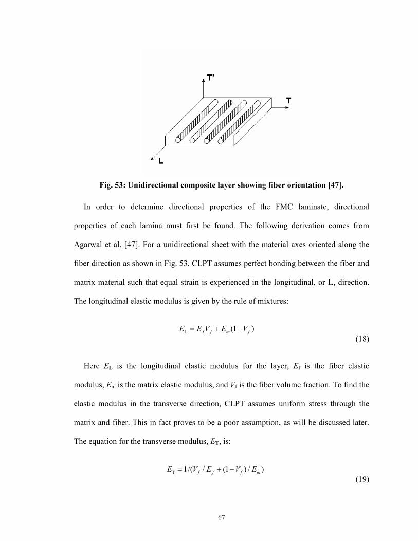
67

Fig. 53: Unidirectional composite layer showing fiber orientation [47].

In order to determine directional properties of the FMC laminate, directional

properties of each lamina must first be found. The following derivation comes from

Agarwal et al. [47]. For a unidirectional sheet with the material axes oriented along the

fiber direction as shown in Fig. 53, CLPT assumes perfect bonding between the fiber and

matrix material such that equal strain is experienced in the longitudinal, or L, direction.

The longitudinal elastic modulus is given by the rule of mixtures:

L (1 )f f m fE E V E V= + − (18)

Here EL is the longitudinal elastic modulus for the layer, Ef is the fiber elastic

modulus, Em is the matrix elastic modulus, and Vf is the fiber volume fraction. To find the

elastic modulus in the transverse direction, CLPT assumes uniform stress through the

matrix and fiber. This in fact proves to be a poor assumption, as will be discussed later.

The equation for the transverse modulus, ET, is:

T 1/( / (1 ) / )f f f mE V E V E= + − (19)

68

Similar expressions can be found for the major Poisson’s ratio, νLT, and shear

modulus, GLT, of a unidirectional fiber lamina. Thus, for each of n orthotropic laminae in

the FMC, numbered from bottom to top, a stiffness matrix [Q] can be determined. Using

the longitudinal modulus from Eq. (18), the transverse modulus from Eq. (19), the shear

modulus, and the major Poisson’s ratio found for each lamina, a compliance matrix [S] is

found, the inverse of which is the lamina stiffness matrix, [Q]:

[ ]

[ ] [ ]

1

1

1

1

0

0

0 0

L LT L

LT L T

LT

E E

S E E

G

Q S

νν

−

−

−

−

−

= −

= (20)

The stiffness matrix [Q] is given in terms of the material axes in Fig. 53. For a

laminate with fiber layers offset from the 1-axis, the stiffness matrix from Eq. (20) must

be transformed to the laminate body axes. From the theory, two standard coordinate

transformation matrices are obtained as a function of the fiber offset angle, θf, yielding an

expression for the lamina stiffness matrix transformed into the laminate body axes:

[ ] [ ][ ]1

1 2( ) ( )Q T Q Tθ θ− =

(21)

Using the transformed stiffness matrix found in Eq. (21) for each lamina k of n

laminae, the directional properties of the laminate can now be calculated. The matrices

[A], [B], and [D] (the extensional stiffness, coupling stiffness, and bending stiffness

matrices, respectively) are determined by summing the weighted laminae stiffnesses

using the following equations:

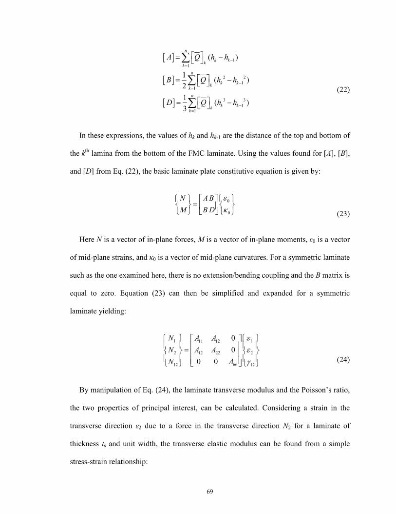
69

[ ]

[ ]

[ ]

1

1

2 2

1

1

3 3

1

1

( )

1( )

2

1( )

3

n

k kk

k

n

k kk

k

n

k kk

k

A Q h h

B Q h h

D Q h h

−=

−=

−=

= −

= −

= −

∑

∑

∑ (22)

In these expressions, the values of hk and hk-1 are the distance of the top and bottom of

the kth lamina from the bottom of the FMC laminate. Using the values found for [A], [B],

and [D] from Eq. (22), the basic laminate plate constitutive equation is given by:

0

0

N AB

M BD

ε

κ

= (23)

Here N is a vector of in-plane forces, M is a vector of in-plane moments, ε0 is a vector

of mid-plane strains, and κ0 is a vector of mid-plane curvatures. For a symmetric laminate

such as the one examined here, there is no extension/bending coupling and the B matrix is

equal to zero. Equation (23) can then be simplified and expanded for a symmetric

laminate yielding:

1 111 12

2 12 22 2

6612 12

0

0

0 0

N A A

N A A

AN

ε

ε

γ

= (24)

By manipulation of Eq. (24), the laminate transverse modulus and the Poisson’s ratio,

the two properties of principal interest, can be calculated. Considering a strain in the

transverse direction ε2 due to a force in the transverse direction N2 for a laminate of

thickness ts and unit width, the transverse elastic modulus can be found from a simple

stress-strain relationship:

70

2 222

2s s

N AE

t tε= =

⋅ (25)

The minor Poisson’s ratio can be found in a similar manner. Consider the ratio of

longitudinal strain ε1 to transverse strain ε2 due to a transverse force N2. The minor

Poisson’s ratio is then given by:

1 2 12 2221

2 2 22 12

/

/

N A A

N A A

εν

ε= = =

(26)

The CLPT method described above was used as a design tool to explore the effects of

different fiber arrangements. Calculations supported the intuitive conclusion that thinner

FMC skins would have a lower in-plane stiffness modulus in the spanwise direction, E2.

Predictions for the transverse elastic modulus from Eq. (25) and the minor Poisson’s ratio

from Eq. (26) are plotted versus fiber offset angle in Fig. 54a and Fig. 54b, respectively,

as solid blue lines. In order to provide some validation for the CLPT predictions, three

FMC sample coupons were manufactured consisting of 0.5 mm elastomer face sheets

sandwiching two 0.2-0.3 mm composite lamina with a fiber volume fraction of 0.7.

Nominal fiber offset angles of 0°, 10°, and 20° were used. The measured transverse

modulus, Fig. 54a, and minor Poisson’s ratio, Fig. 54b, are plotted below as red circles.

It was immediately observed that increasing fiber offset angle adversely increases the

in-plane stiffness of the FMC, requiring greater actuation forces. Also, it is noteworthy

that the inclusion of unidirectional fiber reinforcement at 0° offset angle nearly eliminates

minor Poisson effects.

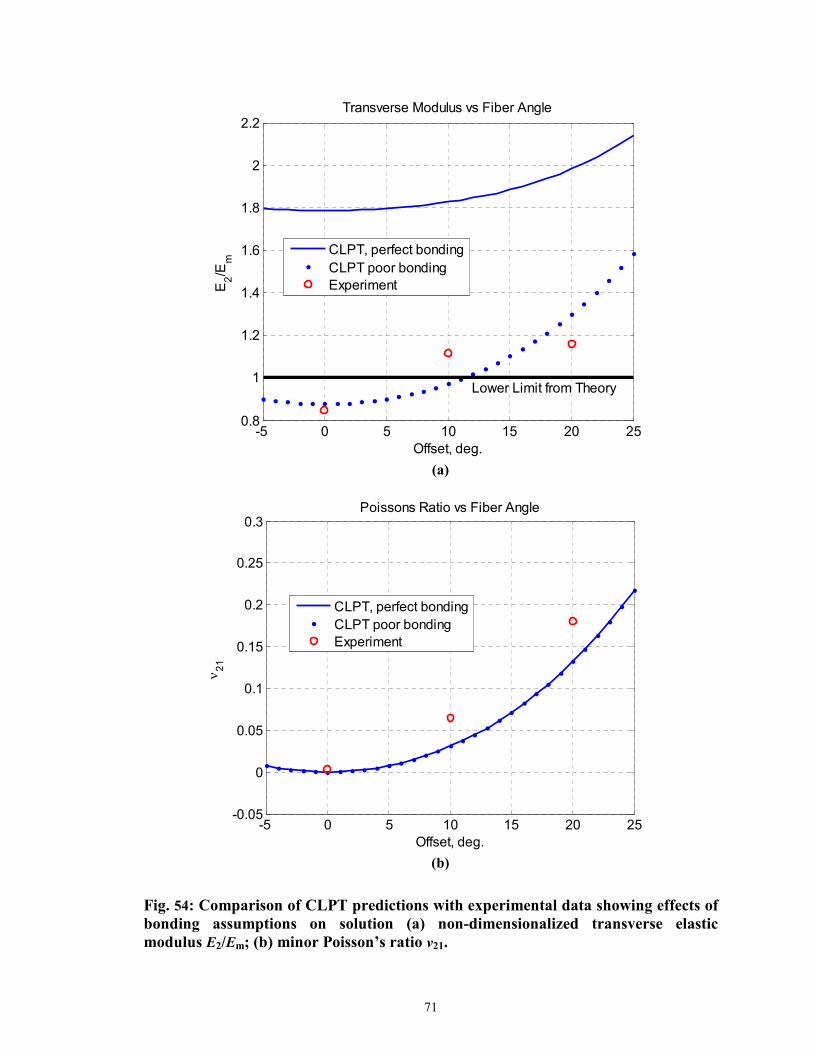
71

-5 0 5 10 15 20 250.8

1

1.2

1.4

1.6

1.8

2

2.2

Offset, deg.

E2/Em

Transverse Modulus vs Fiber Angle

CLPT, perfect bonding

CLPT poor bonding

Experiment

Lower Limit from Theory

(a)

-5 0 5 10 15 20 25-0.05

0

0.05

0.1

0.15

0.2

0.25

0.3

Offset, deg.

ν21

Poissons Ratio vs Fiber Angle

CLPT, perfect bonding

CLPT poor bonding

Experiment

(b)

Fig. 54: Comparison of CLPT predictions with experimental data showing effects of

bonding assumptions on solution (a) non-dimensionalized transverse elastic

modulus E2/Em; (b) minor Poisson’s ratio ν21.

72

It is of critical importance to note that, according to the assumptions used in deriving

the lamina transverse modulus in Eq. (19), the transverse modulus has a lower bound

equal to the matrix modulus. This lower bound is shown in Fig. 54a as a horizontal black

line at E2/Em = 1. However, the experimental data is close to this lower bound for the 10°

and 20° samples, and the modulus is actually below the lower bound for the 0° case.

Clearly there is a problem in the assumptions upon which the transverse modulus

derivation is predicated.

(a) (b)

Fig. 55: Fiber/matrix bond (a) assumed perfect bonding and equal transverse stress

sharing in CLPT; (b) actual condition with poor fiber/matrix bond and no fiber

stress under transverse loading.

Recall it was assumed that perfect bonding between fiber and matrix occurred as

illustrated in Fig. 55a. This implies stress was equally shared between matrix and fiber

under transverse loading. Close visual examination of the FMC samples during testing

revealed that the fiber/matrix bond was actually very poor, and the matrix pulled away

from individual fibers under transverse loading as illustrated in Fig. 55b. Thus, the fibers

carry no stress in the transverse case, and the effective cross-sectional area of matrix left

to carry transverse force in the lamina is reduced by the fiber volume fraction. To account

for this, the transverse modulus in Eq. (19) can be replaced with an expression similar to

73

Eq. (18) by assuming that stress is carried by the matrix alone with a cross sectional area

in proportion to its volume fraction:

T (1 )m fE E V= ⋅ − (27)

Using Eq. (27) in the CLPT calculations greatly reduces the transverse stiffness

contribution of the fiber lamina, making the overall FMC stiffness less than the stiffness

of a solid sheet of matrix material alone at zero degrees fiber angle. Predictions for non-

dimensionalized transverse modulus and minor Poisson’s ratio are plotted in Fig. 54 as

dotted lines. Much better agreement is seen between the analytical and experimental

values for E2/Em.

In spite of the poor bond between fiber and matrix material in the FMCs, the fiber

stiffness still appears to contribute to the transverse stiffness at higher fiber offset angles.

The minor Poisson’s ratio is also influenced by the fiber offset angle, and the FMC’s

longitudinal modulus, not shown, clearly indicates the fiber is contributing to the stiffness

of the laminate. It is hypothesized that friction between fiber and matrix help share load

between the two materials in the longitudinal direction, while the matrix is free to pull

away from the fiber in the transverse direction. This would explain the stiffening effect

seen in the transverse modulus at increased offset angles and the controlling effect the

fiber appears to have on Poisson’s ratio at very low offset angles.

After this correction to the micromechanics assumptions, the CLPT formulation could

be more confidently used to predict FMC directional properties and select a

configuration. Based upon these CLPT results, a fiber offset angle of 0° was selected to

minimize transverse stiffness and also to minimize the minor Poisson’s ratio. As the

74

analytical and experimental results in Fig. 54b indicate, a 0° fiber offset angle can resist

chordwise shape change during spanwise morphing.

3.2.3 FMC Fabrication and Testing

Three FMC samples were manufactured for in-plane testing. First, the outer elastomer

face sheets were pre-cured at room temperature between flat plates spaced to give a

precise thickness of 0.5 mm, as seen in Fig. 56a. Sheets of 0.15 mm thick, 4.1-oz/yd2

(0.014 g/cm2) unidirectional carbon fiber, Fig. 56b, were then prepared by removing the

binder threads which otherwise would adversely affect the transverse stiffness. The

prepared carbon fiber layers and additional uncured elastomer were then sandwiched

between the outer lamina at the appropriate fiber offset angle and cured at room

temperature under a weighted aluminum plate. The result was a continuous elastomer

matrix with layers of fiber embedded in the center at offset angles, shown before being

trimmed to size in Fig. 56c.

(a) (b) (c)

Fig. 56: Manufacturing a ~1.5 mm FMC (a) cured 0.5 mm elastomer sheet; (b) raw

unidirectional carbon fiber; (c) finished FMC sheet, before trimming and clean-up.

The graphics in Fig. 57 describe the three FMC sheets manufactured in an evolving

attempt to maximize in-plane and out-of-plane performance. FMC #1 and FMC #2 had

the same lay-up with two 0.5 mm face sheets sandwiching two 0° offset angle carbon

fiber layers. However, FMC #1 saw an increased effort to control lamina thickness and

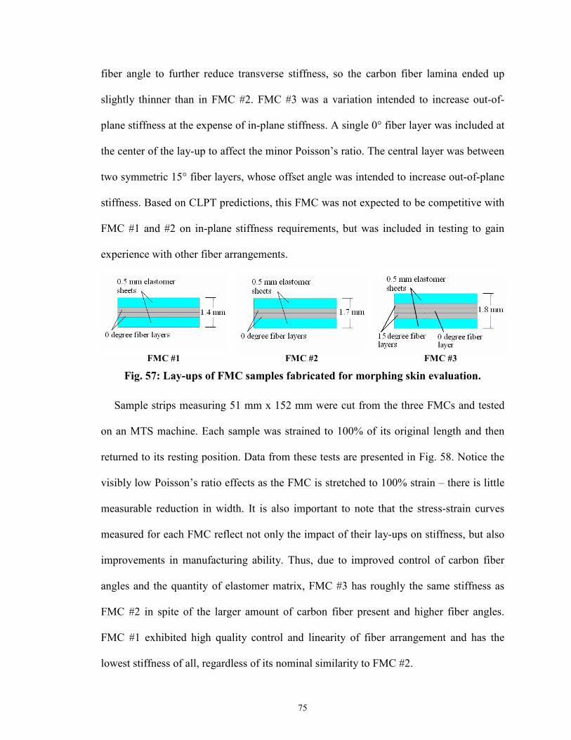
75

fiber angle to further reduce transverse stiffness, so the carbon fiber lamina ended up

slightly thinner than in FMC #2. FMC #3 was a variation intended to increase out-of-

plane stiffness at the expense of in-plane stiffness. A single 0° fiber layer was included at

the center of the lay-up to affect the minor Poisson’s ratio. The central layer was between

two symmetric 15° fiber layers, whose offset angle was intended to increase out-of-plane

stiffness. Based on CLPT predictions, this FMC was not expected to be competitive with

FMC #1 and #2 on in-plane stiffness requirements, but was included in testing to gain

experience with other fiber arrangements.

FMC #1 FMC #2 FMC #3

Fig. 57: Lay-ups of FMC samples fabricated for morphing skin evaluation.

Sample strips measuring 51 mm x 152 mm were cut from the three FMCs and tested

on an MTS machine. Each sample was strained to 100% of its original length and then

returned to its resting position. Data from these tests are presented in Fig. 58. Notice the

visibly low Poisson’s ratio effects as the FMC is stretched to 100% strain – there is little

measurable reduction in width. It is also important to note that the stress-strain curves

measured for each FMC reflect not only the impact of their lay-ups on stiffness, but also

improvements in manufacturing ability. Thus, due to improved control of carbon fiber

angles and the quantity of elastomer matrix, FMC #3 has roughly the same stiffness as

FMC #2 in spite of the larger amount of carbon fiber present and higher fiber angles.

FMC #1 exhibited high quality control and linearity of fiber arrangement and has the

lowest stiffness of all, regardless of its nominal similarity to FMC #2.

76

Based upon these tests, FMC #1 and FMC #2 were selected for incorporation into

integrated test articles. FMC #1 displayed the lowest in-plane stiffness, while FMC #2

had the second lowest stiffness, making them the most attractive candidates for a useful

morphing skin.

(a) (b)

Fig. 58: In-plane skin testing (a) FMC sample taken to 100% strain; (b) data from

FMC samples.

3.3 Substructure Design and Testing

The most challenging aspect of the morphing skin to design was the substructure.

Structural requirements necessitated out-of-plane stiffness sufficient to support the entire

aerodynamic pressure load while still maintaining low in-plane stiffness and high strain

capability.

3.3.1 Honeycomb Design

The substructure concept originally evolved from the use of honeycomb core

reinforcement in composite structures such as rotor blades. Honeycomb structures are

naturally suited for high out-of-plane stiffness, and if properly designed can have tailored

77

in-plane stiffness as well [48]. By modification of the arrangement of a cellular structure,

the desired shape change properties can be incorporated.

In order to achieve a zero Poisson honeycomb structure, a negative Poisson ratio

(auxetic) cellular design presented by Chavez et al. [49] was rearranged to resemble a

series of v-shaped members connecting parallel rib-like structures, as seen in comparison

in Fig. 59. This arrangement gives large strains in one direction with no deflection at all

in the other by means of extending or compressing the v-shaped members.

Fig. 59: Comparison of standard, auxetic, and modified zero-Poisson cellular

structures showing strain relationships.

For a standard honeycomb, Gibson and Ashby [48] describe the in-plane stiffness as a

ratio of in-plane modulus to material modulus, given in terms of the geometric properties

of the honeycomb cells. By modifying this standard equation, it is possible to describe the

in-plane stiffness of a zero-Poisson honeycomb structure with cell geometric properties

as illustrated in Fig. 60. Here t is the thickness of the bending members, ℓ is the length of

the v-shaped bending members, h is the cell height, c is the cell width, and θ is the angle

between the rib members and the bending members. Note that in the figure the cell is

being stretched vertically and F is the force carried by a bending member under tension.

Also note that the depth of the cell, denoted as b, is not represented in Fig. 60.

78

Fig. 60: Geometry of zero-Poisson honeycomb cell.

Fig. 61: Forces and moments on bending member leg.

With the geometry of the cell defined, an expression can be found for the

honeycomb’s equivalent of a stress-strain relationship. For small deflections, the bending

member between points 1 and 2 in Fig. 60 can be considered an Euler-Bernoulli beam as

shown in Fig. 61, with the forces causing a second mode deflection similar to a pure

moment. From Euler-Bernoulli theory, the cosine component of the force F will cause a

bending deflection δ [50]:

79

3

0

cos

12

F

E I

θδ =

�

(28)

Here E0 is the Young’s Modulus of the honeycomb material and I is the second moment

of the area of the bending member; in this case I = bt3/12. In order to determine an

effective stiffness modulus for the honeycomb substructure, the relationship in Eq. (28)

between force and displacement needs to be transformed into an equivalent stress-strain

relationship. The equivalent stress through one cell can be found by using the cell width c

and honeycomb depth b to establish a reference area, and the global equivalent strain is

determined by non-dimensionalizing the v-shaped member’s bending deflection 2δ by the

cell height h. These equivalent stresses and strains are used to determine a stiffness

modulus for the honeycomb, E1:

1 ,F

cbσ =

(29)

1

cos,

/ 2h

δ θε =

(30)

11

1

Eσε

= (31)

Substituting Eqns. (29) through (31) into Eq. (28) and simplifying yields the following

expression for the stiffness of the overall honeycomb relative to the material modulus:

3

1

20

sin

cos

E t

cE l

l

θ

θ

= (32)

80

Because this modified Gibson-Ashby model assumes the bending member legs to be

beams with low deflection angles and low local strains, Eq. (32) should only be valid for

global strains that result in small local deflections. However, it will be shown that due to

the nature of the honeycomb design, relatively large global strains are achievable with

only small local strains.

10 20 30 40 500

.0005

.001

Initial Angle, θ (deg)

Modulus Ratio, E1/E0

Fig. 62: Analytical results for substructure in-plane stiffness.

With this fairly simple equation, the cell design parameters can easily be varied and

their effect on the overall in-plane stiffness of the structure can be studied. For fixed

values of t, h, c, and b, the modulus ratio of the structure, E1/E0, is plotted in Fig. 62 as a

function of the angle θ. As it is shown, smaller angles result in lower in-plane modulus

values. Noting the definitions in Fig. 60, it can be seen that decreasing θ consequently

affects the bending member length l, as the upper and lower ends must meet to form a

viable structure. Thus, for a given cell height h, minimum stiffness limitations are

introduced into the design from a practicality standpoint in that the bending members

81

must connect to the structure and cannot intersect one another. Lower in-plane stiffness

can be achieved by increasing cell width to accommodate lower bending member angles.

Fig. 63: Example of Objet PolyJet rapid-prototyped zero-Poisson honeycomb.

In Fig. 63, an example is given of a zero-Poisson substructure designed in SolidWorks

and produced on an Objet PolyJet rapid prototype machine out of Vero Blue plastic.

Using this method, a large number of samples could be fabricated with variations in

bending member angle, θ. By testing these honeycombs on an MTS machine, a

comparison could be made between the predicted effect of bending member angle on in-

plane stiffness and the actual observed effect.

82

(a) (b)

Fig. 64: Substructure testing (a) substructure on MTS machine; (b) stress-strain

curves of substructures of various interior angles.

The stress-strain test data from a series of rapid prototyped honeycombs is presented

in Fig. 64. Each honeycomb was tested over the intended operating range, starting at 67%

of resting length and extending to 133% of resting length to achieve 100% length change.

To test the validity of the modified Gibson-Ashby model, comparisons of experimental

data and analytical predictions were made. The stiffness modulus of each experimentally

tested honeycomb was determined by applying a linear least squares regression to the

data in Fig. 64. The resulting stiffnesses were then plotted with the analytical predictions

from Eq. (32) in Fig. 65.

83

Fig. 65: In-plane substructure stiffness, analytical versus experiment.

The strong correlation between the analytical predictions and measured behavior

suggests the assumptions made in the modified Gibson-Ashby equation are accurate over

the intended operating range of the honeycomb substructure, and local strains are indeed

relatively low. Having low local strain is a benefit as it will increase the fatigue life of the

substructure. To minimize the in-plane stiffness of the substructure, the lowest

manufacturable bending member angle, 14°, was selected for integration into complete

morphing skin prototypes. Furthermore, this testing demonstrated the usefulness of the

modified Gibson-Ashby equation, Eq. (32), for future honeycomb substructure design

efforts. The in-plane stiffness of zero-Poisson honeycomb structures can be predicted

analytically based upon geometry and material properties.

84

3.3.2 Honeycomb Substructure FEM Analysis

Along with analytical modeling and experimental testing, an FEM analysis of the

zero-Poisson honeycomb substructure was conducted to examine strain behavior.

Specifically, identifying the maximum local strain could be useful for fatigue analysis in

future work. A geometrically nonlinear analysis was conducted on the honeycomb model

shown in Fig. 66 under a prescribed displacement at the top in the z-direction. The

structure was clamped at the bottom and constrained to remain parallel to the x-z plane as

it underwent 76.2 mm (3 in) contraction and extension, equivalent to +/-50% strain. The

honeycomb material, VeroBlue, is isotropic with a Young’s modulus of E = 2.7 GPa and

an assumed Poisson’s ratio ν = 0.3. Ten-node tetrahedral solid elements, provided by a

commercial program, COSMOSDesignSTAR, are used for the analysis.

Fig. 66: Geometry, boundary conditions and meshes for honeycomb model.

85

Fig. 67: Local strain during 30% global compression, max local strain = 1.5%.

The FEM results indicate low local strain for a single bending member compared with

global strain, as Fig. 67 illustrates. The honeycomb sees a maximum local strain of 1.5%

while undergoing 30% compression globally, a 20:1 ratio. This offers hope that a

honeycomb substructure capable of high global strains with a long fatigue life can be

designed by minimizing local strain, an area which should be a topic of further research.

3.3.3 Carbon Fiber Stringers

One unfortunate aspect of the zero-Poisson honeycomb described above is the lack of

bending stiffness about the axis perpendicular to the rib members. Another structural

element is needed to reinforce the substructure for out-of-plane loads. In order to

reinforce the substructure, carbon fiber “stringers” were added perpendicular to the rib

members. Simply comprised of carbon fiber rods sliding into holes in the substructure,

the stringers reinforce the honeycomb against bending about the transverse axis. The

placement of the carbon fiber stringers in the overall morphing skin arrangement is

illustrated in Fig. 68a.

86

(a) (b)

Fig. 68: Reinforced morphing skin cells (a) design of a single cell; (b) interleaving

system arrangement.

Because the stringers are of a fixed length, when the morphing skin is less than fully

extended, they will protrude from the morphing unit. There are a number of possible

ways to mitigate this effect. For example, one concept consists of a system of two

adjacent units with interleaving stringers as in Fig. 68b. When compressed, the stringers

slide into the adjacent unit such that the combined system undergoes 100% shape change

with no fixed length members protruding. Alternatively, for a span-morphing wingtip

comprised of only one morphing unit, the sliding stringers could slide into empty space in

the fixed wing structure when the wingtip is compressed. There are a number of other

suitable ways to address this issue; the selection of a method would depend on the system

integration requirements of a given UAV installation.

3.3.4 FMC/Substructure Adhesive

In order to integrate the FMC face sheets with the honeycomb substructure, a suitable

bonding agent was necessary. The desired adhesive was required to bond the silicone

elastomer FMC to the plastic rapid prototyped honeycomb, while withstanding the shear

forces generated while deforming the structure to high strain levels. In addition, the

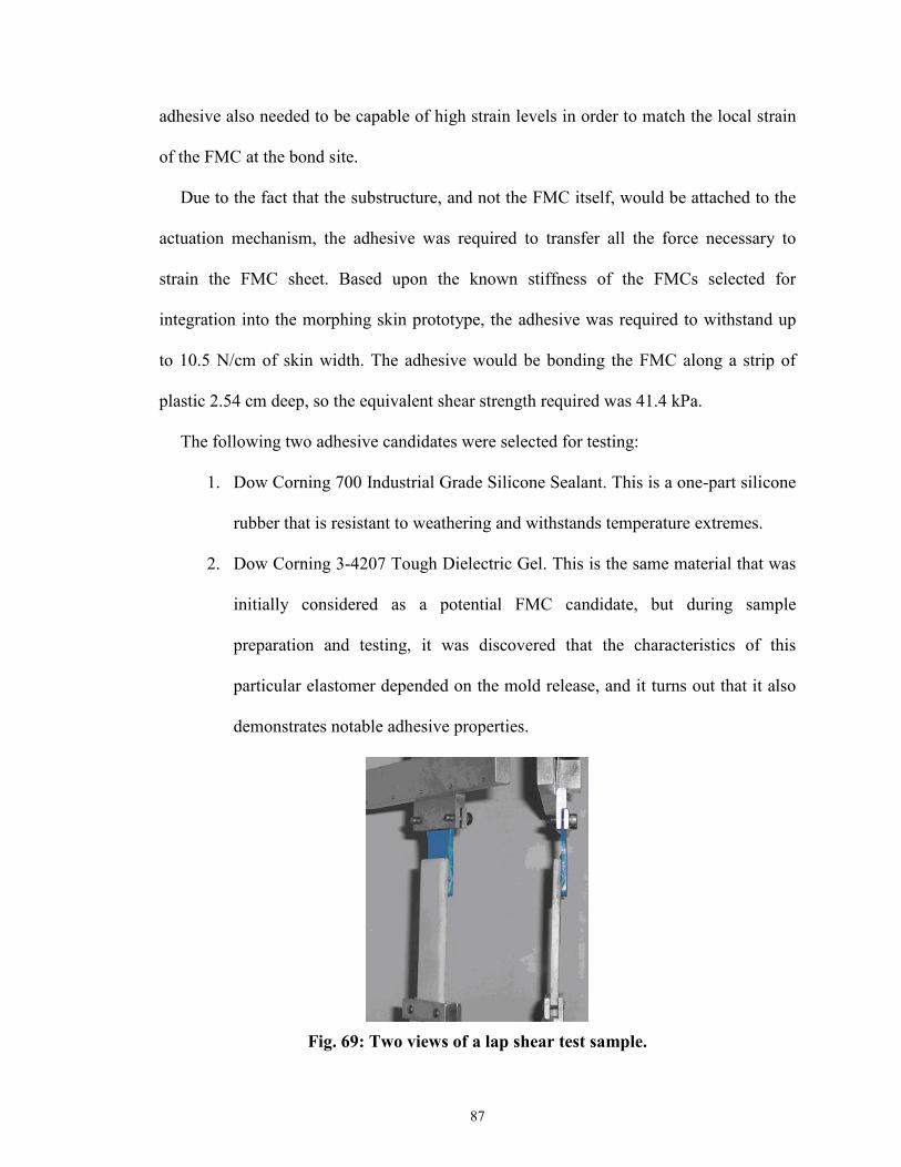
87

adhesive also needed to be capable of high strain levels in order to match the local strain

of the FMC at the bond site.

Due to the fact that the substructure, and not the FMC itself, would be attached to the

actuation mechanism, the adhesive was required to transfer all the force necessary to

strain the FMC sheet. Based upon the known stiffness of the FMCs selected for

integration into the morphing skin prototype, the adhesive was required to withstand up

to 10.5 N/cm of skin width. The adhesive would be bonding the FMC along a strip of

plastic 2.54 cm deep, so the equivalent shear strength required was 41.4 kPa.

The following two adhesive candidates were selected for testing:

1. Dow Corning 700 Industrial Grade Silicone Sealant. This is a one-part silicone

rubber that is resistant to weathering and withstands temperature extremes.

2. Dow Corning 3-4207 Tough Dielectric Gel. This is the same material that was

initially considered as a potential FMC candidate, but during sample

preparation and testing, it was discovered that the characteristics of this

particular elastomer depended on the mold release, and it turns out that it also

demonstrates notable adhesive properties.

Fig. 69: Two views of a lap shear test sample.

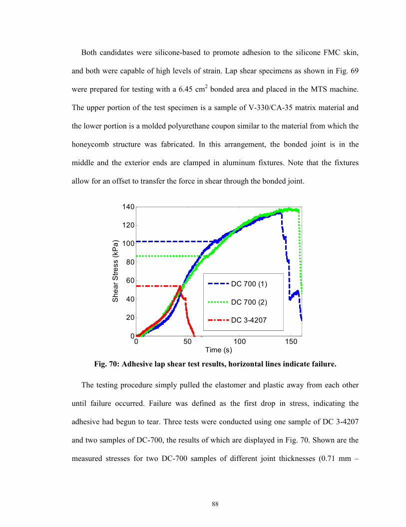
88

Both candidates were silicone-based to promote adhesion to the silicone FMC skin,

and both were capable of high levels of strain. Lap shear specimens as shown in Fig. 69

were prepared for testing with a 6.45 cm2 bonded area and placed in the MTS machine.

The upper portion of the test specimen is a sample of V-330/CA-35 matrix material and

the lower portion is a molded polyurethane coupon similar to the material from which the

honeycomb structure was fabricated. In this arrangement, the bonded joint is in the

middle and the exterior ends are clamped in aluminum fixtures. Note that the fixtures

allow for an offset to transfer the force in shear through the bonded joint.

0 50 100 1500

20

40

60

80

100

120

140

Time (s)

Shear Stress (kPa)

DC 700 (1)

DC 700 (2)

DC 3-4207

Fig. 70: Adhesive lap shear test results, horizontal lines indicate failure.

The testing procedure simply pulled the elastomer and plastic away from each other

until failure occurred. Failure was defined as the first drop in stress, indicating the

adhesive had begun to tear. Three tests were conducted using one sample of DC 3-4207

and two samples of DC-700, the results of which are displayed in Fig. 70. Shown are the

measured stresses for two DC-700 samples of different joint thicknesses (0.71 mm –

89

dashed/blue; 0.64 mm – dotted/green) and one 3-4207 sample of comparable thickness

(0.51 mm – dash-dot/red). Horizontal dotted lines indicate the onset of failure, where the

first reduction in stress occurred. The 3-4207 sample fails before either of the two DC-

700 samples, at a stress of approximately 62 kPa. The thinner sample of DC-700

(dotted/green) fails just above 83 kPa, whereas the thicker sample (dashed/blue) does not

begin to fail until 103 kPa. However, because it would be difficult to precisely control the

bonding layer thickness when attaching the FMC to the honeycomb core, the lowest DC-

700 result (83 kPa) was chosen for comparison to the 3-4207 (62 kPa).

Sufficient evidence was provided in this experiment to demonstrate that the DC-700

was a more suitable adhesive for bonding the FMC elastomer matrix to the modified re-

entrant honeycomb. Not only did the DC-700 fail at a higher stress than the DC 3-4207,

but the initial tear in both DC-700 samples did not immediately propagate through the

adhesive layer. The DC-700 samples continued to carry stress until total failure occurred

at up to half again as high a stress level, giving it a safety factor of approximately 2.

Assuming that future design and manufacturing advances can bring skin stiffness down

even further, the already acceptable safety factor of this adhesive has positive

implications for the safety and reliability for an actual UAV morphing skin application.

3.4 Integration and Final Testing

Two 152 mm x 152 mm morphing skin samples, Skin #1 and Skin #2, were fabricated

from FMC #1 and FMC #2, respectively. VeroBlue 14° angle honeycomb was used for

the substructure for both skins, and DC 700 adhesive was used to bond the two FMCs to

their respective honeycombs. To assist in the attachment, the rib members of the

honeycomb core were designed with raised edges on one side, as shown in Fig. 71a. This

90

figure shows a side view of the zero-Poisson honeycomb, where it can be seen that the

top surface has the ribs extended taller than the bending members. Therefore, the bonding

layer can be applied to the raised rib surfaces and pressed onto the FMC without bonding

the bending members to the FMC. A sectional side view of a single honeycomb cell,

shown in Fig. 71b, illustrates how the bonded morphing skin looks. A thin layer of

adhesive is shown between the FMC and the ribs of the honeycomb, but it does not affect

the movement of the bending members. The first morphing skin sample, Skin #1, was

fabricated using this bonding method.

(a) (b)

Fig. 71: FMC-structure bonding method (a) honeycomb core; (b) single cell

diagram.

A further addition to the substructure reinforcing the FMC sheet was considered for

use in the final test article. This concept employed 1.27 mm carbon fiber rods running

along the rib direction underneath the FMC, placed between each pair of ribs. The

purpose of this concept was to further increase the out-of-plane resistance of the face

sheet by adding rigid members at the point of maximum deflection (center point between

ribs) and provide a means of comparison for Skin #1. The second morphing skin sample,

Skin #2, incorporated added stiffener rods in its construction, shown optionally in Fig.

71b. Silicone adhesive was applied to the FMC to hold the rods in place, although this

proved to be a difficult task and a large amount of adhesive was required to ensure good

91

bonding. The upper and lower surfaces of the assembled Skin #2 sample are displayed in

Fig. 72 in neutral position. The carbon fiber stiffener rods are visible as black lines

parallel to the ribs on the underside of the sheet.

Fig. 72: Completed sample, Skin #2.

The two assembled morphing skin samples were used to assess in-plane and out-of-

plane stiffness and select a morphing skin configuration. The configurations of the two

morphing skins are summarized in Table 2. The selected design was used to fabricate a

final 165 mm x 330 mm test article for combination and evaluation with the actuation

system.

Table 3: Morphing Skin Samples, Summary

Test

Article FMC Honeycomb Adhesive

Additional

Reinforcement

Skin #1

FMC #1, 1.4

mm thick, two

CF layers at 0o

14o zero-Poisson

rapid prototyped

VeroBlue

DC-700 None

Skin #2

FMC #2, 1.7

mm thick, two

CF layers at 0o

14o zero-Poisson

rapid prototyped

VeroBlue

DC-700 Carbon fiber rods

between ribs

92

3.4.1 In-Plane Testing

Skin #1 and Skin #2 were tested on an MTS machine to 50% strain. The level of strain

was limited in order to prevent unforeseen damage to the morphing skins before they

could be tested for out-of-plane stiffness as well. In Fig. 73a, Skin #1 is shown

undergoing testing, with results from both morphing skins presented in Fig. 73b. Note

that the test procedure strained the specimens incrementally, holding the position briefly

before starting with the next stage. This is the cause for the dips in force seen in the

figure.

(a) (b)

Fig. 73: Morphing skin sample in-plane testing (a) assembled skin on MTS; (b) data

from morphing skin in-plane testing.

Skin #2 demonstrated nearly twice the stiffness of Skin #1, which is at least partly due

to the higher stiffness FMC incorporated into Skin #2. However, close examination of the

previously measured stiffnesses of the individual components used in both of these

morphing skins reveals the percentage contribution due to each structural element. These

levels of stiffness contribution are broken down in Fig. 74.

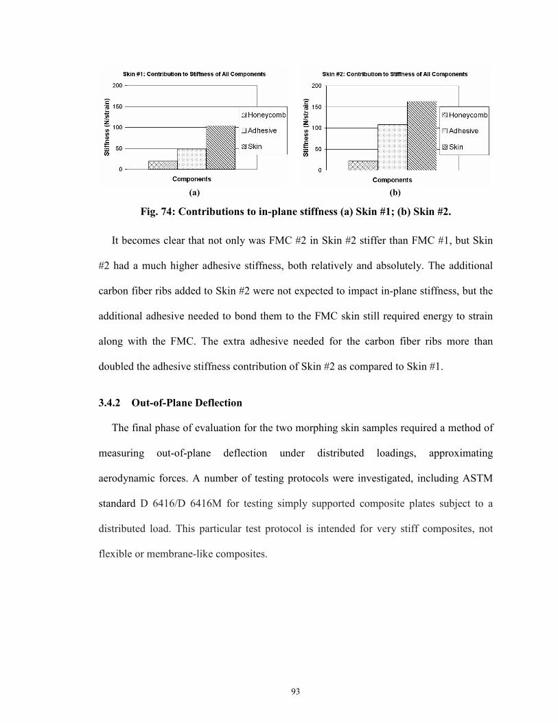
93

(a) (b)

Fig. 74: Contributions to in-plane stiffness (a) Skin #1; (b) Skin #2.

It becomes clear that not only was FMC #2 in Skin #2 stiffer than FMC #1, but Skin

#2 had a much higher adhesive stiffness, both relatively and absolutely. The additional

carbon fiber ribs added to Skin #2 were not expected to impact in-plane stiffness, but the

additional adhesive needed to bond them to the FMC skin still required energy to strain

along with the FMC. The extra adhesive needed for the carbon fiber ribs more than

doubled the adhesive stiffness contribution of Skin #2 as compared to Skin #1.

3.4.2 Out-of-Plane Deflection

The final phase of evaluation for the two morphing skin samples required a method of

measuring out-of-plane deflection under distributed loadings, approximating

aerodynamic forces. A number of testing protocols were investigated, including ASTM

standard D 6416/D 6416M for testing simply supported composite plates subject to a

distributed load. This particular test protocol is intended for very stiff composites, not

flexible or membrane-like composites.

94

Fig. 75: Out-of-plane deflection test apparatus design.

A simpler approach to the problem was adopted wherein acrylic retaining walls were

placed above the morphing skin sample into which a distributed load of lead shot and

sand could be poured. The final configuration of the out-of-plane deflection testing

apparatus can be seen in Fig. 75. A set of lead screws stretched the morphing skin sample

from rest to 100% strain. The acrylic retaining walls could be adjusted to match the active

skin area, and were tall enough to contain lead shot equivalent to a distributed load of 200

psf (9.58 kPa). By applying a thin layer of sand directly to the surface of the skin, the

weight of the lead shot was distributed relatively evenly over the surface of the FMC.

Moreover, as the skin deflected under load, the sand would adjust to conform to the

surface and continue to spread the weight of the lead. A single-point laser position sensor

was also placed underneath to measure the maximum deflections at the center of the skin,

between the rib members. The assembled out-of-plane deflection loading apparatus is

shown in Fig. 76a, with the complete test setup in Fig. 76b.

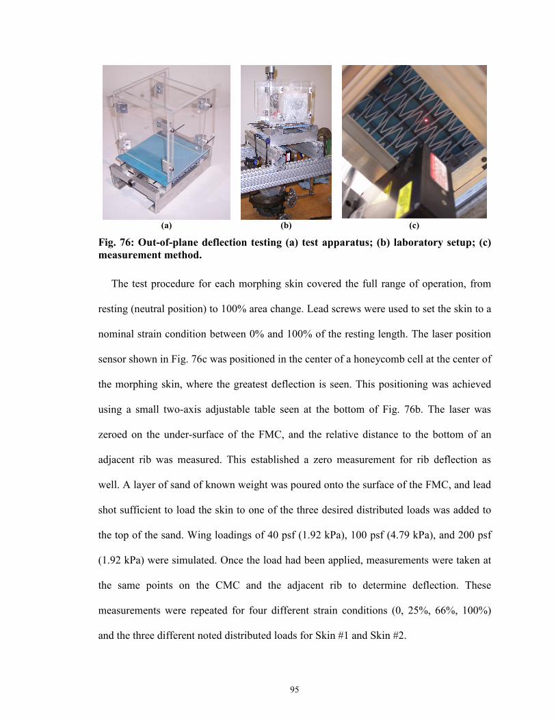
95

(a) (b) (c)

Fig. 76: Out-of-plane deflection testing (a) test apparatus; (b) laboratory setup; (c)

measurement method.

The test procedure for each morphing skin covered the full range of operation, from

resting (neutral position) to 100% area change. Lead screws were used to set the skin to a

nominal strain condition between 0% and 100% of the resting length. The laser position

sensor shown in Fig. 76c was positioned in the center of a honeycomb cell at the center of

the morphing skin, where the greatest deflection is seen. This positioning was achieved

using a small two-axis adjustable table seen at the bottom of Fig. 76b. The laser was

zeroed on the under-surface of the FMC, and the relative distance to the bottom of an

adjacent rib was measured. This established a zero measurement for rib deflection as

well. A layer of sand of known weight was poured onto the surface of the FMC, and lead

shot sufficient to load the skin to one of the three desired distributed loads was added to

the top of the sand. Wing loadings of 40 psf (1.92 kPa), 100 psf (4.79 kPa), and 200 psf

(1.92 kPa) were simulated. Once the load had been applied, measurements were taken at

the same points on the CMC and the adjacent rib to determine deflection. These

measurements were repeated for four different strain conditions (0, 25%, 66%, 100%)

and the three different noted distributed loads for Skin #1 and Skin #2.

96

Skin #1 Skin #2

Fig. 77: Out-of-plane deflection results as measured on the center rib.

Experimental results from the two morphing skins are provided in Fig. 77. It was

observed that, relative to the rib deflections, the FMC sheet itself deflected very little

(less than 0.25 mm). The results in Fig. 77 therefore ignore the small FMC deflections

and show only the maximum deflection measured on the rib at the midpoint of each

morphing skin. Overall, the morphing skin deflections show that as the skin is strained

and unsupported length increases, the out-of-plane deflection increases. Naturally, the

deflection increases with load, as well. This shows that only one condition (maximum

strain, maximum load, on Skin #1) exceeds the specified tolerance of 2.5 mm (10 mil)

deflection.

3.4.3 Full-Scale Integration and Evaluation

Based on the results of the previous two sections, the final skin chosen for

employment in the morphing cell demonstration device was Skin #1, which was shown to

reach over 100% stretch with the lowest in-plane stiffness and largely acceptable out-of-

plane performance. A 34.3 cm x 14 cm morphing skin, nominally identical to Skin #2 in

configuration, was fabricated and attached to the actuation assembly. The actuation

assembly, honeycomb sub-structure, and completed morphing cell can be seen in Fig. 78.

97

Individual components of the system are pictured in Fig. 78a, while the assembled

morphing skin test article appears in Fig. 78b. The active region stretches from 9.1 cm to

18.3 cm with no transverse contraction, thus, producing a 1-D, 100% increase in surface

area with zero Poisson’s ratio.

(a) (b)

Fig. 78: Integration of morphing cell (a) actuation and sub-structure components;

(b) complete morphing cell exhibiting 100% area change.

To characterize the static performance of the morphing cell, input pressure to the PAM

actuators was increased incrementally from approximately 70 kPa to 620 kPa. The strain

of the active region was recorded at each input pressure, and a load cell in line with one

PAM recorded actuator force for comparison to predicted values. This measurement

process was repeated three times, recording strain, input pressure, and actuator force at

each point. Note that the entire upper surface of the FMC is not the active region: each of

the fixed-length ends of the honeycomb was designed and manufactured with 25.4 mm of

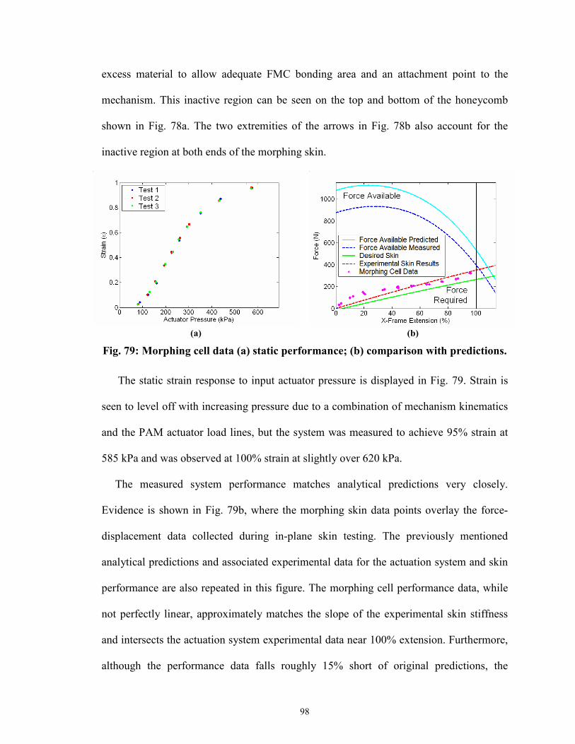
98

excess material to allow adequate FMC bonding area and an attachment point to the

mechanism. This inactive region can be seen on the top and bottom of the honeycomb

shown in Fig. 78a. The two extremities of the arrows in Fig. 78b also account for the

inactive region at both ends of the morphing skin.

(a) (b)

Fig. 79: Morphing cell data (a) static performance; (b) comparison with predictions.

The static strain response to input actuator pressure is displayed in Fig. 79. Strain is

seen to level off with increasing pressure due to a combination of mechanism kinematics

and the PAM actuator load lines, but the system was measured to achieve 95% strain at

585 kPa and was observed at 100% strain at slightly over 620 kPa.

The measured system performance matches analytical predictions very closely.

Evidence is shown in Fig. 79b, where the morphing skin data points overlay the force-

displacement data collected during in-plane skin testing. The previously mentioned

analytical predictions and associated experimental data for the actuation system and skin

performance are also repeated in this figure. The morphing cell performance data, while

not perfectly linear, approximately matches the slope of the experimental skin stiffness

and intersects the actuation system experimental data near 100% extension. Furthermore,

although the performance data falls roughly 15% short of original predictions, the

99

morphing skin meets the design goal, validating the analytical design process. Losses

were not included in the original system predictions. However, the margin of error

included in the original design for friction, increased skin stiffness, and other losses

enabled the final morphing cell prototype to achieve 100% strain. It should also be noted

that 100% area increases could be achieved repeatedly at 1 Hz using manually controlled

actuator pressurization.

3.5 Conclusions

A passive 1-D morphing skin was designed for use on an existing pneumatic actuation

system. The skin consisted of an FMC face sheet with a zero-Poisson honeycomb

substructure intended to support out of plane loads. In-plane stiffness was controlled to

match the capabilities of the actuator by careful design and testing of each separate skin

component. Complete morphing skins were tested for in-plane and out-of-plane

performance and integrated with the actuator to validate the design process.

1. An analytical design procedure was used to size individual morphing skin

components so their combined stiffness matched actuator capabilities. FMC

performance was calculated using classical laminated plate theory with modified

micromechanics, successfully predicting in-plane skin stiffness and Poisson ratio. A

zero-Poisson honeycomb substructure was also designed using a modification to

Gibson and Ashby’s analytical method to accurately predict in-plane stiffness.

2. Using FEM analysis, the local strain in the honeycomb bending members was

determined to be an order of magnitude lower than global strain. For +/-30% global

strain, the maximum local strain was approximately 1.5%. Based on this result, it is

100

expected a zero-Poisson honeycomb can be designed to achieve high strain with a

reasonable fatigue life.

3. A multi-step composite lay-up procedure was developed for fabrication of FMC

skins. The novel procedure relied on the properties of Rhodorsil V-330 CA-35

silicone, in particular the ability to bond pre-cured sheets of V-330 using more V-

330 as the adhesive. This enabled FMC skins to be produced with a continuous

matrix but different fiber volume fractions in distinct lamina, all using a minimum

amount of tooling.

4. Design goals of 100% global strain and 100% area change were demonstrated on a

laboratory prototype using the combined morphing skin and actuation mechanism.

The morphing skin strained smoothly and exhibited a very low in-plane Poisson’s

ratio. Actuation frequencies of roughly 1 Hz were achieved.

101

Chapter 4

Conclusions and Future Work

4.1 Summary of Research and Technical Contributions

The research presented here had two major components which were directed at

developing different aspects of a span morphing wingtip. First a control scheme was

considered and tested in simulation and experiment for a pneumatic artificial muscle

driven extension mechanism. Second a 1-D morphing skin prototype was designed,

fabricated, and demonstrated in operation.

4.1.1 PAM Actuator Controller

In Chapter 2, the effectiveness of controlling a Pneumatic Artificial Muscle actuation

system through linear control was investigated. A Single PAM Test Apparatus was

constructed to provide experimental data over a range of operating conditions against

which modeling efforts could be compared. The actuation system was then modeled in

Simulink as a combination of analytical expressions from theory and lookup tables based

upon characterization of individual components. In particular, the system dynamics and

mass flow of air were handled using well-known equations, while the PAM force and

volume, spring force, and spool valve cross sectional area were described using

experimental data.

Initially, a Simulink model of the pneumatic system was developed and tested against

data captured while charging and exhausting a fixed volume cylinder. A tubing loss term

given by Richer and Hurmuzlu was found to degrade rather than improve model

102

predictions, and was replaced by a pressure drop term from basic hydrodynamic internal

flow which was iterated at each time step. Subsequently, a full dynamic Simulink model

of the actuation system was built and validated using experimental data from the SPTA.

The model showed acceptable performance over a range of conditions, matching the data

qualitatively and in most cases quantitatively as well.

Finally, two linear controllers using displacement feedback were compared in the

Simulink model, one PI and one PID. Ziegler-Nichols tuning was used to determine

controller gains. The PID controller was found to be superior in frequency response and

final waveform shape, and was subsequently implemented on the SPTA test article. The

closed loop experimental system tracked sine inputs with no amplitude attenuation and

little phase lag up to 10 Hz. Tracking of waveforms with higher order harmonics to

simulate aerodynamic control inputs was demonstrated by the model, but in experiment

the PID controller performed poorly at this task, suggesting limitations in the model for

predicting the upper limit on input frequency for the system.

4.1.2 Morphing Skin

In Chapter 3, the proposed morphing skin technology was successfully demonstrated

through design, fabrication, and testing of a morphing skin. Analytical predictions of

FMC in-plane stiffness based on CLPT methods were validated through in-plane testing

of individual FMC skin samples. These predictions aided in selecting a skin configuration

to match in-plane stiffness goals. Analytical methods were also developed to predict in-

plane stiffness of a zero-Poisson honeycomb substructure. Experimental testing of a

range of honeycomb substructures validated the predictions and enabled a minimum

stiffness honeycomb to be selected. Lap shear testing helped select the appropriate

103

adhesive to bond the FMC and substructure based upon ultimate strength requirements.

In-plane and out-of-plane testing of two different morphing skin candidates demonstrated

the viability of the concept by meeting design goals and aided in selecting the best skin

available for production as a full-size test article. Finally, a prototype pneumatic actuation

system was used to demonstrate the ability of a morphing skin panel to achieve 100% 1-

D area change with zero Poisson’s ratio.

4.1.3 Technical Contributions

The controller results are promising in that a major hurdle of employing PAM

actuators, controllability, was overcome for modest frequencies with a linear PID

controller which was simple to tune and implement. Past research which has succeeded at

achieving actuation frequencies greater than 1 Hz has focused exclusively on adaptive or

nonlinear controllers for PAM systems, so that the results of this work are important for

establishing the usefulness and also the limitations of linear controls for PAM actuators.

The main technical contributions of the morphing skin development were two-fold:

first, advancements were made to the methods of reinforcing elastomeric morphing skins

through the use of anisotropic fiber and a novel honeycomb substructure. Specifically,

manufacturing and integration issues were addressed by fabrication a skin panel in a

manner which has not been demonstrated in the literature. Second, the design of this

morphing skin relied on simple analytical methods which were demonstrated to be

effective at predicting in-plane stiffness and which can be applied to future morphing

skins of a similar configuration.

104

4.2 Future Work

The actuation system developed in Chapter 2 was useful as a test article, but is limited

in scope and the results may not be directly applicable to a morphing aircraft design. The

opposing nonlinear spring load on the actuator provides a reasonable approximation of

the work required to strain a morphing skin, but is not representative of the changing

aerodynamic loads a morphing actuation system might encounter on an aircraft. These

loads would depend heavily on the type of craft, the type and design of the morphing

system, and flight conditions, and controller response should be tested under a variety of

more complex simulated loads to ensure a linear controller will be adequate.

Furthermore, while the results presented here encourage interest in the described

control approach, the controlled PAM system response was only simulated in this work.

The immediate next step in developing PAM actuation systems for a morphing craft is

closed loop implementation on the SPTA. Discrepancies between the model and the

physical system could prove significant enough that changes to the controller are

necessary, or could even highlight the need for a more robust controller.

The morphing skin research in Chapter 3 has laid the groundwork for future analytical

design and development of viable morphing structures that are capable of producing

broad-scale area changes and airframe reconfigurations. As described in the motivation of

this research, such skin technology could be useful for a span-changing morphing

aircraft. However, when considering integration of the technology into an aircraft, some

issues must be addressed. First, the prototype system was a simple morphing cell of

rectangular shape. Although this could conceivably illustrate a panel section of a wing, it

is limited in application.

105

Fig. 80: Span extension of wing using airfoil-shaped substructure layer, chordwise

fiber direction.

To increase the potential of this design, alternate implementation strategies should be

examined. The most direct extension of the demonstrated technology is presented in Fig.

80. This concept shows a complete airfoil section that would be supported by a thin

substructure layer, much like the test article described herein. The substructure in this

figure is a zero-Poission honeycomb with airfoil-shaped rib members running along the

chord to produce span extension morphing. The FMC sheet is shown to wrap completely

around the airfoil/honeycomb sub-structure. An actuation system could then be housed

within the hollow section of the airfoil, either the demonstrated pneumatic driven scissor

mechanism or some other type of extension mechanism.

106

Chapter 5

References

[1] Anderson, J. D., Introduction to Flight, 2nd ed., McGraw-Hill, Inc., New York, 1985.

[2] Parker, H. J., “The Parker Variable Camber Wing,” Report #77 Fifth Annual Report, National Advisory

Committee for Aeronautics, Washington, D.C., 1920.

[3] Munk, M. M., “Note on the relative Effect of the Dihedral and the Sweep Back of Airplane Wings,” NACA

Technical Note 177, 1924.

[4] Buseman, A., “Aerodynamic Lift at Supersonic Speeds,” Ae. Techl. 1201, Report No. 2844 (British ARC,

February 3, 1937), Bd. 12, Nr. 6, October, 1935, p. 210-220.

[5] Sarh, B., 1991, “Convertible fixed wing aircraft,” US Patent No. 4,986,493.

[6] Gevers, D. E., 1997, “Multi-purpose aircraft,” US Patent No. 5,645,250.

[7] Blondeau, J. E., and Pines, D. J., “Pneumatic Morphing Aspect Ratio Wing,” 45th AIAA/ASME/ASCE/AHS/ASC

Structures, Structural Dynamics & Materials Conference, 19 - 22 Apr 2004, Palm Springs, CA, Paper No. AIAA

2004-1808.

[8] Toensmeier, P. A., “Morphing Aircraft Could Bring Multi-Role Capability to Next Generation Aircraft,” Aviation

Weekly, May 2005, p. 72-73.

[9] Gern, F. H., Inman, D. J., and Kapania, R.K., “Structural and Aeroelastic Modeling of General Planform Wings

with Morphing Airfoils,” AIAA Journal, 2002, 40(4): 628-637.

[10] Bae, J. S., Seigler, T. M., and Inman, D. J, “Aerodynamic and Static Aeroelastic Characteristics of a Variable-

Span Morphing Wing,” Journal of Aircraft, 2005, 42(2): 528-534.

[11] Henry, J. J., “Roll Control for UAVs by Use of a Variable Span Morphing Wing,” Master’s Thesis, Department of

Aerospace Engineering, University of Maryland, College Park, MD, 2005.

[12] Thill, C., Etches, J., Bond, I., Potter, K., and Weaver, P., “Morphing Skins,” The Aeronautical Journal, Vol. 112,

No. 1129, March 2008, pp 117-139.

[13] Hetrick, J. A., Osborn, R. F., Kota, S., Flick, P. M., and Paul, D. B., “Flight Testing of Mission Adaptive

Compliant Wing,” Proceedings of 48th AIAA Structures, Structural Dynamics, and Materials Conference, 23 - 26

Apr 2007, Honolulu, HI, Paper No. AIAA 2007-1709.

107

[14] Perkins, D. A., Reed, J. L., and Havens, E., “Morphing Wing Structures for Loitering Air Vehicles,” 45th AIAA

Structures, Structural Dynamics & Materials Conference, 19-22 April 2004, Palm Springs, CA, Paper No. AIAA

2004-1888.

[15] Bye, D. R., and McClure, P. D., “Design of a Morphing Vehicle,” 48th AIAA Structures, Structural Dynamics, and

Materials Conference, 23 - 26 Apr 2007, Honolulu, HI, Paper No. AIAA 2007-1728.

[16] Kikuta, M. T., “Mechanical Properties of Candidate Materials for Morphing Wings,” Master of Science Thesis,

Virginia Polytechnic Institute and State University, Blacksburg, VA, 2003.

[17] Flanagan, J., Strutzenberg, R., Myers, R., and Rodrian, J., “Development and Flight Testing of a Morphing

Aircraft, the NextGen MFX-1” Proceedings of 48th AIAA Structures, Structural Dynamics, and Materials

Conference, 23 - 26 Apr 2007, Honolulu, HI, Paper No. AIAA 2007-1707.

[18] Wereley, N. M. and Kothera, C. S., “Morphing Aircraft Using Fluidic Artificial Muscles,” Proceedings of the

International Conference on Adaptive Structures and Technologies, 2-5 Oct 2007, Ottawa, ON, Paper ID 171.

[19] Caldwell, D.G., Medrano-Cerda, G.A., and Goodwin, M., “Control of Pneumatic Muscle Actuators,” IEEE

Control Systems, Feb 2005, pp 40-48.

[20] Medrano-Cerda, G.A., Bowler, C.J., and Caldwell, D.G., "Adaptive position control of antagonistic pneumatic

muscle actuators," IEEE/RSJ International Conference on Intelligent Robots and Systems, Vol. 1, No. 1, Aug

1995.

[21] Kothera, C.S., Jangid, M., Sirohi, J., and Wereley, N.M., 2006, “Experimental Characterization and Static

Modeling of McKibben Actuators,” ASME International Mechanical Engineering Congress and Exposition, 5-10

Nov 2006, Chicago, IL, Paper No. IMECE2006-15390.

[22] Gentry, M. F., and Wereley, N. M., “Effects of Braid Angle on Pneumatic Artificial Muscle Actuator

Performance,” Proceedings of the ASME Conference on Smart Materials, Adaptive Structures and Intelligent

Systems, 28-30 Oct 2008, Ellicott City, MD, Paper No. SMASIS2008-539.

[23] Nickel, V., et al., 1965, “Synthetically Powered Orthotic Systems,” Journal of Bone and Joint Surgery, Vol. 47-B,

Aug 1965, pp 458-464.

[24] Tondu, B. and Pierre, L., “Modeling and Control of McKibben Artificial Muscle Robot Actuators,” IEEE Control

Systems Magazine, Apr 2000, pp 15-38.

[25] Schroder, J., Erol, D., Kawamura, K., and Dillman, R., "Dynamic pneumatic actuator model for a model-based

torque controller," Proceedings 2003 IEEE International Symposium on Computational Intelligence in Robotics

and Automation., Vol. 1, 16-20 Jul 2003, pp. 342-347.

108

[26] Paul, A.K., Mishra, J.K., and Radke, M.G., “Reduced Order Sliding Mode Control for Pneumatic Actuator,” IEEE

Transactions on Control Systems Technology, Vol. 2, No. 3, Sept 1994.

[27] Richer, E., and Hurmuzlu, Y., “A High Performance Pneumatic Force Actuator System: Part II – Nonlinear

Controller Design,” ASME Journal of Dynamic Systems, Measurement, and Control, Vol. 122 Sept 2000, pp. 426-

434.

[28] Khalil, H. K., Nonlinear Systems, Prentice Hall, Upper Saddle River, 2002.

[29] Hildebrandt, A., Sawodny, O., Neumann, R., and Hartmann, A., “A Flatness Based Design for Tracking Control

of Pneumatic Muscle Actuators,” Seventh International Conference on Control, Automation, Robotics and Vision,

Singapore, Dec 2002.

[30] van der Linde, R.Q., “Design, Analysis, and Control of a Low Power Joint for Walking Robots, by Phasic

Activation of McKibben Muscles,” IEEE Transactions on Robotics and Automation, Vol. 15, No. 4, Aug 1999.

[31] Chou, C.P., and Hannaford, B., “Measuring and Modeling of McKibben Pneumatic Artificial Muscles,” IEEE

Transactions on Robotics and Automation, Vol. 12, No. 1, Feb 1996.

[32] Gaylord, R., 1958, “Fluid actuated motor system and stroking device,” US Patent No. 2,844,126.

[33] Richer, E., and Hurmuzlu, Y., “A High Performance Pneumatic Force Actuator System: Part I – Nonlinear

Mathematical Model,” ASME Journal of Dynamic Systems, Measurement, and Control, Vol. 122 Sept 2000, pp.

416-425.

[34] Al-Ibrahim, A. M., and Otis, D. R., “Transient Air Temperature and Pressure Measurements During the Charging

and Discharging Processes of an Actuating Pneumatic Cylinder,” Proceedings of the 45th National Conference on

Fluid Power, 1992.

[35] Beater, P., Pneumatic Drives: System Design, Modelling, and Control, Springer, New York, 2007.

[36] Burrows, C. R., and Peckham, R. G., “Dynamic characteristics of a pneumatic flapper valve,” Proc Instn Mech

Engrs, Journal of Mechanical Engineering Science, Vol. 19(3), Part C, pp. 113-121.

[37] Pugi, L., Malvezzi, M., Allotta, B., Banci, L., Prescniani, P., “A parametric library for the simulation of a Union

Internationale des Chemins de Fer (UIC) pneumatic braking system,” Proc Instn Mech Engrs, Journal of Rail and

Rapid Transit, Vol. 218, Part F, pp. 117-132.

[38] Carducci, G., Giannoccaro, N. I., Messina, A., and Rollo, G., “Identification of viscous friction coefficients for a

pneumatic system model using optimization methods,” Mathematics and Computers in Simulation 71, 2006, pp

385-394.

109

[39] Incropera, F. P., and DeWitt, D. P., Fundamentals of Heat and Mass Transfer, John Wiley & Sons, New York,

2006.

[40] Ziegler, J. G., and Nichols, N. B., “Optimum settings for automatic controllers,” ASME Transactions, Vol. 64,

1942, pp. 759-768.

[41] Shen, J., Yang, M., and Chopra, I., “Swashplateless Helicopter Rotor with Trailing-Edge Flaps for Flight and

Vibration Control,” AIAA/ASME/ASCE/AHS/ASC 45th Structures, Structural Dynamics and Materials

Conference, Palm Springs, CA, 2004.

[42] Hess, R. A., “Structural Model of the Adaptive Human Pilot,” AIAA Journal of Guidance and Control, Vol. 3, No.

5, 1980, pp 416-423.

[43] Nieuwenhuizen, F. M., Beykirch, K. A., Mulder, M., Bulthoff, H. H., “Identification of Pilot Control Behavior in a

Roll-Lateral Helicopter Hover Task,” AIAA Modeling and Simulation Technologies Conference, 20 - 23 Aug

2007, Hilton Head, SC, Paper No. AIAA 2007-6799.

[44] Theodore, C. R., Tischler, M. B., Colbourne, J. D., “Rapid Frequency Domain Modeling methods for UAV Flight

Control Applications,” AIAA Atmospheric Flight Mechanics Conference and Exhibit, 11-14 Aug 2003, Austin,

TX, Paper No. AIAA 2003-5538.

[45] Murray, G., Gandhi, F., and Bakis, C., “Flexible Matrix Composite Skins for One-Dimensional Wing Morphing,”

Proceedings of 48th AIAA Structures, Structural Dynamics, and Materials Conference, 23 - 26 Apr 2007,

Honolulu, HI, Paper No. AIAA 2007-1737.

[46] Olympio, K. R., "Design of a passive flexible skin for morphing aircraft structures," M.S. Thesis, Pennsylvania

State University, 2006.

[47] Agarwal, B. D., Broutman, L. J., and Chandrashekhara, K., Analysis and Performance of Fiber Composites, John

Wiley & Sons, Hoboken, 2006.

[48] Gibson, L. J. and Ashby, M. F., Cellular Solids: Structure and Properties, Pergamon Press, Oxford, 1988.

[49] Chaves, F. D., Avila, J., and Avila, A. F., “A morphological study on cellular composites with negative Poisson’s

ratios,” Proceedings of 44th AIAA Structures, Structural Dynamics, and Materials Conference, 7-10 Apr 2003,

Norfolk, VA, Paper No. AIAA 2003-1951.

[50] Shigley, J., Mishke, C., and Budynas, R., Mechanical Engineering Design, McGraw-Hill, New York, 2004.

ABSTRACT HIGHLY EXTENSIBLE SKIN FOR A VARIABLE WING …

Documents

Transcript of ABSTRACT HIGHLY EXTENSIBLE SKIN FOR A VARIABLE WING …