ABSTRACT

Title of Dissertation: Cosmological Probes ofPhysics Beyond the Standard Model

Soubhik KumarDoctor of Philosophy, 2020

Dissertation Directed by: Professor Raman SundrumDepartment of Physics

The Standard Model (SM) of particle physics can explain a diverse variety of

experimental observations. However, there remain multiple compelling reasons why

we believe that the SM is not the final theory of the universe. In this thesis, we first

briefly discuss some of those shortcomings of the SM, and then focus on ways in

which cosmological observations can be used to probe theories beyond the SM. The

primary probe we consider for this purpose is primordial non-Gaussianity (NG) of

cosmological perturbations. We show that by precise studies of NG we can probe

ultra-high energy gauge theories that might otherwise be energetically completely

inaccessible to terrestrial experiments, by focusing first on (i) generic spontaneously

broken Higgsed gauge theories, and then on, (ii) higher-dimensional Grand Unified

Theories (GUTs). Building upon this, we also discuss a simple curvaton extension

of the standard inflationary paradigm where strength of various NG signals can be

orders of magnitude larger, and thus be easily accessible via observations in the

coming decade.

Cosmological Probes ofPhysics Beyond the Standard Model

by

Soubhik Kumar

Dissertation submitted to the Faculty of the Graduate School of theUniversity of Maryland, College Park in partial fulfillment

of the requirements for the degree ofDoctor of Philosophy

2020

Advisory Committee:Professor Raman Sundrum, Chair/AdvisorProfessor Kaustubh AgasheProfessor Zackaria ChackoProfessor Anson HookProfessor Richard Wentworth

c© Copyright bySoubhik Kumar

2020

Dedication

To Ma, Baba and Titas.

ii

Acknowledgments

My Ph.D. journey has been far from a solo one, and this is a great opportunity

to thank all the friends, family, teachers, and collaborators whose support made this

thesis possible.

I would like to start by thanking my advisor, Prof. Raman Sundrum. His

deep insights, vast knowledge, and clarity of thought are only some of the many

other qualities that have continually inspired me. I especially want to thank him for

spending countless hours discussing physics with me, and his willingness to patiently

listen to my thoughts, even when they were ill-formed. I also greatly admire his

willingness and infectious enthusiasm to jump into less familiar but exciting areas

of research and this is something I will take with me as I continue in my research

career. Away from academic life, he has been an exemplary human being showing

empathy and care for my personal life as well. I hope to have him as a mentor and

collaborator in the years to come.

I would also like to thank Prof. Kaustubh Agashe. I have been fortunate

enough to regularly interact with him over these years and collaborate on ideas

related to extra dimensions. His enthusiasm and thoroughness have been very in-

spiring as well. I will always appreciate his willingness to answer questions, often in

a very careful and detailed manner. At the same time, his probing questions often

forced me to think more carefully about seemingly simple ideas, and in the end,

enriched my understanding.

Prof. Zackaria Chacko has been very influential right from the start of my

iii

graduate school. His Quantum Field Theory lectures were the ones through which I

got introduced to some of the core ideas of the subject, and I deeply appreciate the

clarity of his lectures. Although he was not my official advisor, he regularly cared

about my progress. His advice on various aspects of academic life, both pertaining

to research and more general aspects, has been very valuable.

Prof. Anson Hook has been a continual source of exciting new ideas that

made many lunches and other informal discussions so much fun. I had the chance

of collaborating with him on axion physics and hope to continue that in the future.

His way of simplifying problems and quick back-of-the-envelope estimations have

been an inspiration.

I would also like to thank Prof. Paulo Bedaque, Prof. Alessandra Buonanno,

Prof. Thomas Cohen, Prof. Zohreh Davoudi, Prof. Bei-Lok Hu, Prof. Ted Jacobson,

Prof. Xiangdong Ji and Prof. Rabi Mohapatra for enjoyable discussions during these

years. I am also greatly indebted to Prof. Richard Wentworth along with Profs.

Sundrum, Agashe, Chacko, and Hook for agreeing to serve on my thesis committee

and spending their invaluable time to review this thesis.

I have been very fortunate to have wonderful collaborators from whom I

learned a lot. I thank Arushi Bodas, Kaustubh Deshpande, Peizhi Du, Majid

Ekhterachian, Zhen Liu, Yuhsin Tsai for their time, discussions and continued col-

laborations.

Enormous thanks are also due to past and present students and post-docs

at Maryland for lots of fun discussions. They include Stefano Antonini, Dawid

Brzeminski, Dan Carney, Jack Collins, David Curtin, Saurav Das, Abhish Dev,

iv

Sanket Doshi, Reza Ebadi, Anton de la Fuente, Michael Geller, Sungwoo Hong,

Chang Hun Lee, Rashmish Mishra, Arif Mohd, Simon Riquelme, Prashant Saraswat,

Antony Speranza, Gustavo Marques Tavares, Christopher Verhaaren, Yixu Wang

among others. I would also like to thank all the participants of TASI 2018 for

making it so memorable.

I would also like to thank everyone at IISER-Kolkata for all their help during

my undergraduate days, and especially, my undegraduate thesis guide Prof. Ritesh

K. Singh for his kind mentoring and many insightful physics discussions.

Thanks are also due to Heather Markle and Melanie Knouse for making various

administrative processes so smooth at Maryland Center for Fundamental Physics

(MCFP).

My friends Sabyasachi, Sarthak, Tamoghna, Subhojit, Subhayan along with

others made life at College Park super enjoyable. Special thanks goes to Sabyasachi

for tolerating me as a housemate for this entire duration. My old friends Abhijit

and Suvadip were, as usual, omnipresent and responsible for lots of fun whenever I

had the chance to visit India.

None of this would have been possible without the generous support, love, and

care of my parents. They were the first ones to encourage me to pursue physics

and no words are enough to express my gratitude towards them. They will always

remain two of the strongest pillars of my life.

Titas has been a constant ray of sunshine ever since she came into my life.

Although often she was physically a few hundred miles away, her encouragement,

love, and care became only closer as the days passed. I owe so much of my well-being

v

to her.

I would also like to acknowledge the help and financial support from MCFP,

National Science Foundation (NSF), University Fellowship, Dean’s Fellowship, Mon-

roe H. Martin Graduate Research Fellowship, and Professor C H Woo Award in

Nuclear and Particle Theory during my graduate study.

It is impossible to remember everyone and any omission reflects my sloppiness,

not your deeply-valued friendship. Thank you!

vi

Table of Contents

Dedication ii

Acknowledgements iii

Table of Contents vii

List of Tables x

List of Figures xi

1 Introduction 11.1 The Standard Model and the need to go beyond it . . . . . . . . . . . 11.2 Cosmic inflation . . . . . . . . . . . . . . . . . . . . . . . . . . . . . . 51.3 Primordial non-Gaussianity . . . . . . . . . . . . . . . . . . . . . . . 121.4 Outline of the thesis . . . . . . . . . . . . . . . . . . . . . . . . . . . 14

2 Heavy-Lifting of Gauge Theories By Cosmic Inflation 172.1 Introduction . . . . . . . . . . . . . . . . . . . . . . . . . . . . . . . . 172.2 Preliminaries . . . . . . . . . . . . . . . . . . . . . . . . . . . . . . . 27

2.2.1 The in-in Formalism for Cosmological Correlators . . . . . . . 272.2.2 Useful Gauges for General Coordinate Invariance . . . . . . . 282.2.3 Observables . . . . . . . . . . . . . . . . . . . . . . . . . . . . 31

2.3 Squeezed Limit of Cosmological Correlators . . . . . . . . . . . . . . 332.3.1 NG from Single Field Inflation in the Squeezed Limit . . . . . 332.3.2 NG from Multifield Inflation in the Squeezed Limit . . . . . . 362.3.3 NG from Hubble-scale Masses in the Squeezed Limit . . . . . 36

2.4 Gauge-Higgs Theory and Cosmological Collider Physics . . . . . . . . 402.4.1 The Central Plot and its Connections to the Literature . . . . 402.4.2 High Energy Physics at the Hubble Scale . . . . . . . . . . . . 432.4.3 Heavy-lifting of Gauge-Higgs Theory . . . . . . . . . . . . . . 46

2.5 NG in Single Field Slow Roll Inflation . . . . . . . . . . . . . . . . . 472.5.1 Cutoff and Coupling Strengths of Effective Theory . . . . . . 482.5.2 Visibility of a Higgs Scalar . . . . . . . . . . . . . . . . . . . . 512.5.3 Visibility of a Massive Gauge Boson . . . . . . . . . . . . . . . 542.5.4 Gauge Theory with a Heavy Higgs Scalar . . . . . . . . . . . . 57

2.6 NG in the Effective Goldstone Description of Inflationary Dynamics . 58

vii

2.6.1 Minimal Goldstone Inflationary Dynamics . . . . . . . . . . . 592.6.1.1 Leading Terms in the Effective Theory and Power

Spectrum . . . . . . . . . . . . . . . . . . . . . . . . 592.6.1.2 Higher Order Terms . . . . . . . . . . . . . . . . . . 65

2.6.2 Incorporating Gauge-Higgs Theory into the Goldstone Effec-tive Description . . . . . . . . . . . . . . . . . . . . . . . . . . 672.6.2.1 Visibility of a Higgs Scalar . . . . . . . . . . . . . . . 672.6.2.2 Visibility of a Massive Gauge Boson . . . . . . . . . 69

2.7 Detailed Form of NG Mediated by h . . . . . . . . . . . . . . . . . . 712.7.1 Single Exchange Diagram . . . . . . . . . . . . . . . . . . . . 722.7.2 Double Exchange Diagram . . . . . . . . . . . . . . . . . . . . 742.7.3 Triple Exchange Diagram . . . . . . . . . . . . . . . . . . . . 76

2.8 Detailed Form of NG Mediated by Z . . . . . . . . . . . . . . . . . . 792.8.1 Single Exchange Diagram . . . . . . . . . . . . . . . . . . . . 812.8.2 Double Exchange Diagram . . . . . . . . . . . . . . . . . . . . 82

2.9 Concluding Remarks and Future Directions . . . . . . . . . . . . . . . 83

3 Seeing Higher-Dimensional Grand Unification in Primordial Non-Gaussianities 883.1 Introduction . . . . . . . . . . . . . . . . . . . . . . . . . . . . . . . . 883.2 Orbifold GUTs and Gauge Coupling Unification . . . . . . . . . . . . 97

3.2.1 Orbifold GUTs . . . . . . . . . . . . . . . . . . . . . . . . . . 973.2.2 Gauge Coupling Unification . . . . . . . . . . . . . . . . . . . 99

3.3 Non-gaussianity and Massive Particles . . . . . . . . . . . . . . . . . 1013.4 Inflation and the Fifth Dimension . . . . . . . . . . . . . . . . . . . . 103

3.4.1 General Set-up . . . . . . . . . . . . . . . . . . . . . . . . . . 1033.4.1.1 Gravitational Fluctuations . . . . . . . . . . . . . . . 105

3.4.2 Semi-Infinite Extra Dimension . . . . . . . . . . . . . . . . . . 1073.4.2.1 Background Solution and the Horizon . . . . . . . . 1083.4.2.2 KK Graviton Wavefunction . . . . . . . . . . . . . . 109

3.4.3 Introduction of the Second Boundary . . . . . . . . . . . . . . 1113.4.3.1 Radion Mass and Stabilization . . . . . . . . . . . . 1113.4.3.2 Near-horizon Analysis of Stabilization . . . . . . . . 113

3.4.4 Inflationary Couplings . . . . . . . . . . . . . . . . . . . . . . 1183.4.4.1 Wavefunction of KK Graviton on Inflationary Bound-

ary . . . . . . . . . . . . . . . . . . . . . . . . . . . . 1183.4.4.2 Coupling of KK Graviton to the Inflaton . . . . . . . 1213.4.4.3 Estimate of NG Mediated by KK Graviton . . . . . . 122

3.5 Gauge Theory States . . . . . . . . . . . . . . . . . . . . . . . . . . . 1253.5.1 KK Analysis of 5D Gauge Theory . . . . . . . . . . . . . . . . 1253.5.2 Contribution of KK Gauge Boson to NG . . . . . . . . . . . . 128

3.5.2.1 SO(10) GUT in the Bulk . . . . . . . . . . . . . . . 1303.5.2.2 SU(5) GUT in the Bulk . . . . . . . . . . . . . . . . 133

3.6 Detailed Form of NG Mediated by Spin-2 . . . . . . . . . . . . . . . . 1343.7 Detailed Form of NG Mediated by Spin-1 . . . . . . . . . . . . . . . . 1353.8 Conclusion and Future Directions . . . . . . . . . . . . . . . . . . . . 137

viii

4 Cosmological Collider Physics and the Curvaton 1414.1 Introduction . . . . . . . . . . . . . . . . . . . . . . . . . . . . . . . . 1414.2 Observables and cosmological collider physics . . . . . . . . . . . . . 1474.3 Curvaton paradigm . . . . . . . . . . . . . . . . . . . . . . . . . . . . 149

4.3.1 Cosmological history . . . . . . . . . . . . . . . . . . . . . . . 1494.3.2 Observational constraints . . . . . . . . . . . . . . . . . . . . . 154

4.4 Charged heavy particles in the standard inflationary paradigm . . . . 1584.4.1 Higgs exchange in the broken phase . . . . . . . . . . . . . . . 1594.4.2 Charged scalar exchange in the symmetric phase . . . . . . . . 1614.4.3 Charged Dirac fermion . . . . . . . . . . . . . . . . . . . . . . 163

4.5 Charged heavy particles in the curvaton paradigm . . . . . . . . . . . 1654.5.1 Higgs exchange in the broken phase . . . . . . . . . . . . . . . 1704.5.2 Charged scalar exchange in the symmetric phase . . . . . . . . 1724.5.3 Charged Dirac fermion . . . . . . . . . . . . . . . . . . . . . . 173

4.6 Conclusions and future directions . . . . . . . . . . . . . . . . . . . . 175A.1 Scalar Fields in dS Space . . . . . . . . . . . . . . . . . . . . . . . . . 178

A.1.1 Massive Fields . . . . . . . . . . . . . . . . . . . . . . . . . . . 178A.1.2 Inflaton Mode Functions . . . . . . . . . . . . . . . . . . . . . 181A.1.3 Some Useful Relations for Diagrammatic Calculations . . . . . 181

A.2 NG due to h Exchange . . . . . . . . . . . . . . . . . . . . . . . . . . 182A.2.1 Calculation of Single Exchange Diagram . . . . . . . . . . . . 182

A.2.1.1 Calculation of I+− . . . . . . . . . . . . . . . . . . . 184A.2.1.2 Calculation of I−− . . . . . . . . . . . . . . . . . . . 186A.2.1.3 Three-Point Function . . . . . . . . . . . . . . . . . 187

A.2.2 Calculation of Double Exchange Diagram . . . . . . . . . . . . 188A.2.2.1 Mixed Propagators . . . . . . . . . . . . . . . . . . . 188A.2.2.2 Three-Point Function . . . . . . . . . . . . . . . . . 190

A.2.3 Calculation of Triple Exchange Diagram . . . . . . . . . . . . 192A.3 Massive Vector Fields in dS Space . . . . . . . . . . . . . . . . . . . . 193

A.3.1 Mode Functions in Momentum Space . . . . . . . . . . . . . . 193A.4 NG due to Z Exchange . . . . . . . . . . . . . . . . . . . . . . . . . . 195B.1 KK Reduction of the Graviton-Radion System . . . . . . . . . . . . . 199B.2 NG Mediated by the KK Graviton . . . . . . . . . . . . . . . . . . . 202

B.2.1 Mode Functions for Helicity-0 component of a Massive Spin-2Field in dS4 . . . . . . . . . . . . . . . . . . . . . . . . . . . . 203

B.2.2 Calculation of Single Exchange Diagram . . . . . . . . . . . . 205C.1 Charged scalar loop . . . . . . . . . . . . . . . . . . . . . . . . . . . . 210C.2 Fermion loop . . . . . . . . . . . . . . . . . . . . . . . . . . . . . . . 212

Bibliography 214

ix

List of Tables

2.1 NG mediated by h via single exchange diagram in effective Goldstonedescription. . . . . . . . . . . . . . . . . . . . . . . . . . . . . . . . . 72

2.2 NG mediated by h via single exchange diagram in single-field slow-rollinflation. . . . . . . . . . . . . . . . . . . . . . . . . . . . . . . . . . . 74

2.3 NG mediated by h via double exchange diagram in effective Goldstonedescription. . . . . . . . . . . . . . . . . . . . . . . . . . . . . . . . . 75

2.4 NG mediated by h via double exchange diagram in single-field slow-roll inflation. . . . . . . . . . . . . . . . . . . . . . . . . . . . . . . . 76

2.5 NG mediated by h via triple exchange diagram in effective Goldstonedescription. . . . . . . . . . . . . . . . . . . . . . . . . . . . . . . . . 77

2.6 NG mediated by h via triple exchange diagram in single-field slow-rollinflation. . . . . . . . . . . . . . . . . . . . . . . . . . . . . . . . . . . 78

2.7 NG mediated by Z via single exchange diagram in effective Goldstonedescription. . . . . . . . . . . . . . . . . . . . . . . . . . . . . . . . . 81

2.8 Summary of strength of NG mediated by h and Z. . . . . . . . . . . 84

x

List of Figures

1.1 The motion of the inflaton field φ on an inflationary potential V (φ).After slowly rolling in the region labelled as “slow-roll inflation”,the inflaton field reaches the region labelled as “reheating” whereit oscillates around the minima of the potential and decays into SMradiation bath giving rise to a radiation dominated Universe. Theclassical dynamics of this evolution is controlled by the homogeneouspart φ0(t) of the inflaton field. The observed density perturbationsin the reheated Universe, on the other hand, comes from its quantummechanical fluctuations, ξ(t, ~x). . . . . . . . . . . . . . . . . . . . . . 5

2.1 From left to right: (a) Tree level exchange of neutral massive scalar (inred) between inflatons (in black); (b) Loop level exchange of chargedmassive fields (in blue) between inflatons (in black). The externallines are taken to end at the end of inflation, conformal time, η ≈ 0. . 20

2.2 NG in single-field inflation . . . . . . . . . . . . . . . . . . . . . . . . 342.3 Non-Gaussianity due to Massive Particles . . . . . . . . . . . . . . . . 382.4 From left to right: (a) “OPE” approximation of three point function

in squeezed limit as a two point function. The φ0 background causingmixing is not explicitly shown, as in Fig. 2.3. (b) The same “OPE”approximation expressed an inflaton-h three point function with oneinflaton leg set to zero momentum to now explicitly represent thebackground φ0. . . . . . . . . . . . . . . . . . . . . . . . . . . . . . . 38

2.5 Dimensionless three-point function F singleh (2.23) for different masses

in Goldstone Effective description (104) with λ2 = 0.2;λh = 0.5; Λ =8H. . . . . . . . . . . . . . . . . . . . . . . . . . . . . . . . . . . . . . 73

2.6 Shape sensitivity of F singleh to mh. We have chosen three plausible

sets of parameters for which F singleh agree at the fiducial ratio k1

k3= 5.

This illustrates our ability to discriminate among different masses. . . 732.7 Dimensionless three-point function F single

h (2.23) for different masses

in Single-field Slow-roll description (103) with c2 = H√φ0, λh = H2

2φ0,Λ =

3

√φ0. . . . . . . . . . . . . . . . . . . . . . . . . . . . . . . . . . . . 75

2.8 Shape sensitivity of F singleh to mh. We have chosen three plausible

sets of parameters for which F singleh agree at the fiducial ratio k1

k3= 5.

This illustrates our ability to discriminate among different masses. . . 76

xi

2.9 Dimensionless three-point function F doubleh (2.23) for different masses

in Goldstone Effective description (117) with λ2 = 0.2;λh = 0.5. . . . 772.10 Shape sensitivity of F double

h to mh. We have chosen three plausiblesets of parameters for which F double

h agree at the fiducial ratio k1k3

= 5.This illustrates our ability to discriminate among different masses. . . 78

2.11 Dimensionless three-point function F tripleh (2.23) for different masses

in Goldstone Effective description (121) with λ2 = 0.2;λh = 0.5. . . . 792.12 Shape sensitivity of F triple

h to mh. We have chosen three plausible sets

of parameters for which F tripleh agree at the fiducial ratio k1

k3= 5. This

illustrates our ability to discriminate among different masses. . . . . . 80

3.1 SM Renormalization Group Evolution (RGE) of gauge couplings giat 1-loop written in terms of αi ≡ g2

i /4π. The label “i = 1,2,3”denotes the U(1) , SU(2) and SU(3) SM subgroups respectively withthe normalization that g1 =

√5/3g′ where g′ is the SM hypercharge

coupling. . . . . . . . . . . . . . . . . . . . . . . . . . . . . . . . . . . 883.2 5D spacetime having two boundaries at y = 0 and y = L. (a) Dirich-

let Boundary Conditions (BC’s) on the gauge bosons of GUT/SMachieves the breaking G→ SM on the left boundary, also housing theinflaton φ(x). Neumann BC’s on all gauge bosons preserve G on theright boundary. . . . . . . . . . . . . . . . . . . . . . . . . . . . . . . 90

3.3 Tree level contributions to bispectrum due to massive particle ex-change. From left to right: (a) single exchange diagram, (b) doubleexchange diagram, (c) triple exchange diagram. All the three dia-grams depend on the mixing between the massive particle (in red)and the inflaton fluctuation (in black) in the (implicit) non-trivialbackground of slowly rolling φ0(t). η is (conformal) time, ending atthe end of inflation. . . . . . . . . . . . . . . . . . . . . . . . . . . . . 92

3.4 Same set-up as in Fig. 3.2 except the right boundary is absent anda “black brane” horizon has formed due to the backreaction of theinflationary vacuum energy on the left boundary. . . . . . . . . . . . 94

3.5 Strength of NG mediated by spin-2 KK graviton for tensor-to-scalarratio r = 0.1 and KK wavefunction on inflationary boundary ψ(0) =1. Such strengths for the range of masses shown are observable withincosmic variance (see Section 3.3) . . . . . . . . . . . . . . . . . . . . . 135

3.6 Strength of NG mediated by spin-1 KK gauge bosons for inflaton-KKmixing ρ = 0.3 and derivative of KK wavefunction on the inflationaryboundary ϑ′(0) = 1. Such strengths for the range of masses shownare observable within cosmic variance (see Section 3.3) . . . . . . . . 137

xii

4.1 Various energy scales discussed in this chapter. H and Mpl are re-

spectively, the inflationary Hubble scale and the Planck scale. V1/4

inf

and

√φ0 are respectively the potential and kinetic energy scales of

the inflaton field. Similarly, V1/4σ and

√σ0 are respectively the po-

tential and kinetic energy scales of the curvaton field. A sample setof values of the above scales can be obtained using the benchmarkparameter point given in eq. (4.31). . . . . . . . . . . . . . . . . . . . 143

4.2 Massive Higgs mediated (in red) tree level “in-in” contributions to theinflaton (in black) three point function. Depending on the number ofmassive scalar propagators, these diagrams are labelled from left toright: (a) single exchange diagram, (b) double exchange diagram, (c)triple exchange diagram. η denotes conformal time which ends at theend of inflation. . . . . . . . . . . . . . . . . . . . . . . . . . . . . . . 160

4.3 Massive charged particle mediated (in red) loop level “in-in” contri-butions to the inflaton (in black) three point function. Depending onthe number of massive charged particle propagators, these diagramsare labelled from left to right: (a) double exchange diagram, (b) tripleexchange diagram. η denotes conformal time which ends at the endof inflation. . . . . . . . . . . . . . . . . . . . . . . . . . . . . . . . . 162

4.4 The strength of NG for tree level Higgs exchange as a function ofHiggs mass mχ for ρ2 = 0.3H and σ0 = −H2. The function |fχ,tree(µ)|is defined in eq. (4.62). . . . . . . . . . . . . . . . . . . . . . . . . . . 171

4.5 The strength of NG for loop level scalar exchange as a function ofscalar mass mχ for Λσ = 4H and σ0 = −H2. The function |fχ,loop(µ)|is defined in eq. (4.66). . . . . . . . . . . . . . . . . . . . . . . . . . . 173

4.6 The strength of NG for loop level charged fermion exchange as afunction of fermion mass mΨ for Λσ = 4H and σ0 = −H2. Thefunction |fΨ,loop(µ)| is defined in eq. (4.70). . . . . . . . . . . . . . . . 175

7 Reduction of a loop diagram into a linear combination of tree dia-grams in the squeezed limit. . . . . . . . . . . . . . . . . . . . . . . . 211

xiii

Chapter 1: Introduction

1.1 The Standard Model and the need to go beyond it

The Standard Model (SM) of particle physics (for a review see [1]) has been

a crowning achievement in all of physics, and perhaps, in all of science. SM can

explain a variety of experimental observations spanning across more than 40 orders

of magnitude in scales, from hundredths of a femtometer to tens of Gigaparsecs.

However, there are compelling reasons to believe that this is not the end of the

story.

Various gravitational observations, including the Cosmic Microwave Back-

ground (CMB), suggest that around 85 percent of all matter and around 26 percent

of all energy density in the present Universe, consists of the so called Dark Matter

(DM), see e.g. [2]. The SM does not give us any clue about what constitutes the

DM and whether/how it interacts non-gravitationally with the rest of the SM. Sim-

ilarly mysterious is the nature of Dark Energy which constitutes, an even bigger,

68 percent of the energy density of the present Universe, see e.g. [2]. At the same

time, the SM does not explain the origin of the observed tiny neutrino masses [3].

Furthermore, in the Universe around us, we see more matter than antimatter. The

SM does not provide a dynamical mechanism by which such a matter-antimatter

1

asymmetry could have been generated starting from a symmetric initial state.

Apart from these observational puzzles, there remain some striking conceptual

puzzles about the SM as well. In 2012, we discovered the Higgs boson at the Large

Hadron Collider (LHC) [4, 5]. Through the mechanism of spontaneous symmetry

breaking, the Higgs boson plays a crucial role in SM by giving masses to almost

all the elementary particles of the SM. Although we have measured the mass of

the Higgs boson to be around 125 GeV, we do not know the fundamental origin of

the Higgs boson and where its mass and self-coupling comes from. Thus, a theory

beyond the SM that dynamically explains the mass and the coupling of the Higgs

boson is required to truly understand the masses of elementary particles around

us. In fact, various beyond the SM theories, where we can calculate the Higgs

mass from first principles, often predict a Higgs mass hierarchically larger than its

observed value of 125 GeV, giving rise to the so called Higgs Hierarchy Problem.

Another conceptual puzzle is related to the strength of observed coupling pa-

rameters in the strong, weak and electromagnetic interactions. According to the SM,

these three coupling parameters seem to “unify” around a very high energy scale of

1013−14 GeV. Just as how Maxwell’s theory unified electricity and magnetism, and

the electroweak theory unified electromagnetism with weak interactions, SM does

give hints that the electroweak and the strong interactions might also get unified

into a Grand Unified Theory (GUT) at those very high scales [6]. While we do not

know the possibility of such a grand unification for certainty as of now, an answer

is very much desirable.

The set of exciting questions above gives us strong reasons to believe that there

2

is physics beyond the SM (BSM). The important question that we can then ask is:

what are the most theoretically plausible BSM scenarios that are also experimentally

testable in the near future? The LHC, starting more than a decade ago, has been

playing a driving role in this regard since it is probing physics at multi-TeV scales,

particularly relevant for the Hierarchy Problem. While it has not given us any

strong hints of BSM physics as yet, with its various detector upgrades for its “High-

Luminosity” phase [7], it will be able to gather more than 10 times the data it has

obtained till now with much more precision. Thus it is very much possible that

exciting discoveries could be around the corner. Apart from that, in recent years

a variety of novel experimental ideas probing physics at energies much lower than

the TeV scale, has emerged, especially in the context of DM, and more generally,

Dark Sectors, that very weakly interact with the SM, but can share many of its

complexities.

While the progress to understand the physics at TeV scales or below has

been phenomenal, we can also wonder about how to experimentally/observationally

probe BSM physics operating at scales much bigger than a TeV. There are indeed

several well-motivated BSM theories that are believed to operate at such high scales,

one example being GUTs mentioned above. Since such GUTs can easily exist at

energies 10 orders of magnitude above that accessible by the LHC — the highest

energy particle collider build to date — at first sight it seems impossible that we

can probe such very high-scale theories.

The primary focus of this thesis is to demonstrate how we can use cosmological

observables, especially Primordial Non-Gaussianity (NG), to directly probe precisely

3

those high-scales theories. We will make a crucial use of the fact that currently, our

best developed theory, that explains the structure of the Universe at large scales,

strongly suggests an early period of Cosmic Inflation during which the early Universe

underwent a very energetic expansion. In general, the expansion of the Universe can

be characterized by the Hubble parameter, H, as will be described below. Current

CMB observations indicate that Hubble scale during inflation could have been as big

as 5×1013 GeV [8]. With the aid of this large energy scale H, the rapidly expanding

Universe could have cosmologically produced ultra-heavy particles with masses ∼

H. Once produced, these particles, via their decay into inflationary field(s) that

determine density perturbations, can leave their distinctive features, such as their

masses and spins, in the NG of CMB and in the distribution of galaxies forming Large

Scale Structure (LSS) — giving us a unique probe of BSM physics operating at very

high scales. While at present, the observed spectrum of primordial perturbations is

purely Gaussian, in the coming decade, we will have significant improvement in NG

measurements, most notably using LSS (see e.g. [9]), and perhaps also from 21-cm

cosmology experiments probing cosmic dark ages, spanning redshifts of z ∼ 30−100

(see e.g. [10, 11]). Therefore by studying CMB, LSS and 21-cm cosmology, we can do

on-shell spectroscopy of ultra-heavy particles that are otherwise inaccessible. Before

getting on to main part of the thesis, let us briefly review some of the essential

concepts.

4

Figure 1.1: The motion of the inflaton field φ on an inflationary potential V (φ).After slowly rolling in the region labelled as “slow-roll inflation”, the inflaton fieldreaches the region labelled as “reheating” where it oscillates around the minima ofthe potential and decays into SM radiation bath giving rise to a radiation domi-nated Universe. The classical dynamics of this evolution is controlled by the homo-geneous part φ0(t) of the inflaton field. The observed density perturbations in thereheated Universe, on the other hand, comes from its quantum mechanical fluctua-tions, ξ(t, ~x).

1.2 Cosmic inflation

The observed Universe is extremely homogeneous and isotropic on large scales.

However on smaller scales, we also observe inhomogeneities and anisotropies via

CMB and LSS. An era of cosmic inflation in the very early Universe is the leading

paradigm to explain both these features of the observed Universe on large and small

scales [12, 13, 14]. For a review of cosmic inflation, see [15]. The simplest models of

inflation postulate a scalar field, the inflaton φ, that slowly rolls along its almost-

flat potential during inflation as shown in fig. 1.1. While this slow-roll takes place,

the potential energy density of the inflaton remains almost constant at a positive

value, and consequently, the Universe undergoes a rapid expansion and thereby

dilutes any prior “irregularities” of spacetime. As a result, the large-scale Universe

becomes extremely homogeneous and isotropic. As shown in fig. 1.1, in simplest

5

models of inflation, the inflaton eventually reaches a minima of its potential around

which it starts a rapid oscillation. This marks the end of the inflationary phase.

During that oscillation, through its coupling to the SM fields, the inflaton can decay

into SM radiation bath and the Universe gets reheated into a radiation dominated

era.

Importantly, the inflaton φ also fluctuates quantum mechanically during this

entire period. The quantum fluctuations generated during the inflationary period

get stretched out to very large scales. Those fluctuations then source the inhomo-

geneities and anisotropies in the radiation-dominated reheated Universe. As the

Universe keeps evolving, such fluctuations determine the anisotropies in CMB and

eventually, via gravitational clustering form the LSS. We now give a very brief

overview of inflationary dynamics, which will be treated in more detail in Chapter

2, to make some of the above statements more precise.

The general metric describing a 3+1 dimensional expanding, homogeneous and

isotropic spacetime, characterized by coordinates (t, ~x), can be written as

ds2 = −dt2 + a(t)2d~x2 = a2(η)(−dη2 + d~x2). (1.1)

Here t and η are cosmic and conformal times respectively, related to each other by

dη = dta(t)

; and a(t) is the scale factor that governs the spacetime expansion. The

Hubble parameter H(t),

H(t) =da(t)/dt

a(t), (1.2)

6

characterizes the rate at which the spacetime expands. The coupled classical dy-

namics of the inflaton field φ and the metric is governed by the equation of motion

of the scalar field and the Friedmann equation which are respectively given by,

φ+ 3Hφ+ V′′(φ) = 0, (1.3)

1

2φ2 + V (φ) = 3H2M2

pl, (1.4)

where an overdot denotes a derivative with respect to t. The Planck scale Mpl is

determined by the Gravitational constant GN via M2pl ≡ 1/(8πGN). During slow-roll

inflation, φ2 V (φ), and eq. (1.4) shows that H approximately remains constant.

Using eq. (1.2) we then see that the scale factor grows exponentially during inflation,

i.e., a(t) ∼ eHt. The conformal time η then goes as,

η ∼ − 1

Ha. (1.5)

The end of inflation corresponds to an exponentially large value of the scale factor

compared to its initial value and is reached when |ηe| |η|CMB where ηCMB is

a time scale when a typical fluctuation mode, later observed via CMB, exit the

horizon during inflation. To denote its smallness, we will take the time for the end

of inflation, ηe ≈ 0. As far as the classical evolution of the inflaton field is concerned,

such a rapid expansion makes the Universe homogeneous and isotropic on largest

of scales as mentioned earlier. However, its quantum evolution is more subtle and

that gives rise to anisotripies and inhomogenities on smaller scales. We turn to this

7

next.

An enormous success of the inflationary paradigm is that it predicts some of

the crucial qualitative properties of the observed density perturbations in CMB and

LSS. To investigate this we need to consider the fluctiations of the inflaton field

which can be written as,

φ(t, ~x) = φ0(t) + ξ(t, ~x), (1.6)

where φ0(t) and ξ(t, ~x) are the classical slowly rolling inflaton field and its quantum

fluctuation respectively. In general, to study the evolution of ξ(t, ~x) we need to

consider the scalar fluctuations of the metric as well. However, for the purposes in

this thesis where we will mostly be interested in calculating heavy-particle induced

NG, such metric fluctuations can be ignored in the leading slow-roll approximation,

as will be discussed in Chapter 2. Thus the leading dynamics of ξ can be analyzed

as if it is a quantum field in the unbackreacted spacetime geometry given by eq.

(1.1). Then the equation of motion of ξ, after Fourier transforming to 3-momentum

space, is given by,

∂2ηξ −

2

η∂ηξ + k2ξ = 0, (1.7)

where we have neglected the potential of the inflaton field which is a valid approxi-

mation during slow-roll inflation. Here ~k is the “comoving” momentum, conjugate

to ~x in eq. (1.1), and it remains constant in time as the spacetime expands. Its

8

magnitude is denoted by k. Eq. (1.7) can be solved as,

ξ(η,~k) ∼ H

k3/2(1± ikη)e∓ikη. (1.8)

Here, the overall normalization factor of 1/k3/2 has been fixed by noting that as

η → −∞, eq. (1.7) can be reduced to an equation of motion of a harmonic oscillator

by rewriting it in terms of the variable ξ/η. Thus the solution in eq. (1.8) should also

have the usual 1/k1/2 normalization, as appropriate to a haromic oscillator mode

function, in η → −∞ limit.

Importantly, from eq. (1.8), we see as a fluctuating k−mode evolves to a super-

horizon scale characterized by |kη| 1, it stops evolving in time and freezes to some

constant non-zero value determined by its dynamics during inflation. When such

fluctuating modes reenter our horizon during a much later era, they restart their

evolution with the same conserved value and eventually seed the density pertur-

bations. Although we do not have a complete observational picture of the early

Universe between temperatures ∼ MeV and inflationary scales, which could be as

high as 1013−14 GeV, this super-horizon conservation implies that any unknown

dynamics at intermediate scales, especially during reheating, can not affect the evo-

lution of large-scale primordial perturbations. This is the primary reason why we

can still infer about primordial physics at inflationary scales from observations of

CMB and LSS without having a detailed idea of physics at intermediate scales.

The basic idea behind cosmological particle production can also be obtained

from eq. (1.7). By rewriting it in terms of the variable, ϕ = ξ/(ηH), we obtain the

9

equation of motion of a harmonic oscillator,

ϕ′′ +

(k2 − 2

η2

)ϕ = 0, (1.9)

with a time-dependent frequency ω2 = k2 − 2η2

. The existence of such a time-

dependent frequency indicates a time-dependent Hamiltonian, and thus, the vacuum

state of the theory at time η1 is different from that at some other time η2. Now

suppose the Universe started from a vacuum state |Ω〉 at very early times 1. Focusing

on the Heisenberg picture for a moment, at some later time ηlate the Universe will

still be in the same state |Ω〉. However, due to the time-dependent Hamiltonian,

the instantaneous vacuum state at ηlate would be |Ω〉late 6= |Ω〉. Since in this case

late〈Ω|Ω〉 6= 0, the Universe would contain particles from the perspective of the

vacuum at ηlate. In other words, cosmological particle production due to a time-

dependent background has taken place.

While our primary concern in this thesis will be analyzing non-Gaussianity me-

diated by heavy particles, it is worth quickly sketching how (almost) scale-invariant

Gaussian primordial perturbations arise in minimal inflationary models. To do this

we can first construct the power spectrum of ξ 2,

〈ξ(ηe, ~k)ξ(ηe,−~k)〉. (1.10)

1The description of how to choose such a “Bunch-Davies” vacuum state is described in chapter 2.2We will, for the moment, neglect the fact that ξ is not a gauge invariant quantity when

the metric is treated fully dynamically. A gauge invariant observable characterizing NG will beconstructed in Chapter 2.

10

Here we are evaluating the two point correlation function at some late time ηe ≈ 0

towards the end of inflation, by when all the inflaton fluctuations have exited the

horizon and become frozen in time. The spatial momenta of the two fluctuations are

given by ±~k due to momentum conservation. Further details regarding how exactly

such two point (and higher-point, in general) correlation functions are defined and

computed will be reviewed in Chapter 2. Now using eq. (1.8), we see that the

two-point function goes as,

〈ξ(ηe, ~k)ξ(ηe,−~k)〉|ηe→0 ∼H2

k3. (1.11)

By Fourier transforming this momentum-space answer, one sees that the position

space two point function is scale-invariant, upto almost constancy of H during in-

flation. A gauge invariant form of the power spectrum will be given in Chapter

2.

A simple way by which a statistical distribution of a given observable can

be non-Gaussian (NG) is by developing a non-zero three-point correlation function

which would have otherwise vanished if the distribution were Gaussian. Therefore,

one way of characterizing NG is by computing three-point correlation functions of

inflaton fluctuations, ξ:

〈ξ(ηe, ~k1)ξ(ηe, ~k2)ξ(ηe, ~k3)〉. (1.12)

Here the spatial momenta of the fluctuations are denoted by ~ki for i = 1, 2, 3. In min-

11

imal inflationary models, the interactions of the inflaton field is very small, and hence

any odd-point correlation function of ξ, in particular, 〈ξ(ηe, ~k1)ξ(ηe, ~k2)ξ(ηe, ~k3)〉 is

small as well [16]. Furthermore, all even-point correlation functions are mostly de-

termined in terms of the two-point function. Thus the minimal inflationary models

predict an approximately Gaussian spectrum of primordial perturbations.

Having obtained some insight about the dynamics of primordial perturbations,

let us now discuss the primary cosmological observable of interest that we will re-

peatedly use in this thesis, namely primordial non-Gaussianity. While four and

higher-point correlation functions are also sensitive probes of non-Gaussianity, in

this thesis, we will focus on the three-point function as a concrete example.

1.3 Primordial non-Gaussianity

Inflaton self-interactions, and more excitingly, interactions of the inflaton with

other fields that could be present during inflation, can easily make the three-point

function large so that it can be observable in CMB and LSS. This is especially

important from a BSM point of view once we remember that the Hubble scale

during inflation can be as big as 5×1013 GeV [8]. Thus by studying such three-point

functions, and more generally NG, one can investigate particle physics operating at

energy scales as much as 10 orders of magnitude larger than what can be done at

the LHC for example. What makes this even more striking is the observation that if

there were particles having masses ∼ H interacting with the inflaton, they can get

produced during inflation and leave their on-shell mass and spin information in such

12

NG correlators [17, 18, 19, 20, 21]. It is this fact that the study of NG using CMB,

LSS and 21-cm cosmology can let us do spectroscopy of ultra-high energy particle

physics, which are otherwise completely inaccessible, that will be the recurring theme

of this thesis. Since this process of extraction such on-shell particle properties using

cosmology is similar in spirit to what is done at terrestrial colliders, such as the LHC,

the above-mentioned paradigm has been dubbed as Cosmological Collider Physics

[21].

Before giving an outline of the thesis, we pause to comment on two important

observational aspects. Through out our discussion of NG, we will ignore the so-called

“secondary” NG that the density perturbations develop as they grow under the

effect of gravitational clustering, for a review see e.g. [22]. While such secondaries

are extremely important from an observational point of view, in this thesis, we will

assume that they can be modeled sufficiently well so that the primordial, inflationary

contributions can be reliably extracted from the data and our conclusions can then

be immediately applied. The second issue has to do with the precision by which

NG can be measured. Such a precision, quite generally, improves as 1√N

as the

number of independent measurements of the observable, N , is increased. Therefore,

the best sensitivity to primordial NG will come from cosmic-variance limited 21-cm

cosmology observations probing cosmic dark ages, spanning redshifts z ∼ 30− 100,

since those can probe orders of magnitude more number of cosmological modes

compared to CMB and LSS [23]. While for some of the conclusions obtained in

this thesis, CMB and especially, LSS will be sufficient, for several others, 21-cm

observatons will be of critical importance. We will give a rough estimate of the

13

sensitivity of such 21-cm observations in chapter 2.

1.4 Outline of the thesis

Having described the basic idea behind the inflationary paradigm and pri-

mordial NG from in a broad-brush manner, we will review it more rigorously in

Chapter 2 which is based upon [24]. Following that, we extend the Cosmological

Collider Physics program to investigate the observability of generic spontaneously

broken Higgsed gauge theories for the first time in literature. By carefully impos-

ing the constraints of gauge symmetry and its (partial) Higgsing, we identify that

two different types of Higgs mechanisms can lead to observable NG signals. In the

first category, the Higgs scale is constant before and after inflation, and one can

observe NG effects of particles much heavier than those accsessible by laboratory

experiments, as mentioned above. In the second category, which we dub as the

“Heavy-lifting” scenario, the Higgs scale is determined by the curvature of space-

time and is time-dependent. Correspondingly we show how particles which are light

in the current era, can nonetheless get heavy-lifted to inflationary energy scale and

give non-trivial NG signals. Utilizing this feature, we show how NG can be used as

a novel test of the severity of the Higgs Hierarchy Problem mentioned earlier.

We then move to Chapter 3, based upon [25], where we evaluate under what

conditions GUTs can lead to observable NG signatures, demonstrating a unique

direct probe of GUTs known in the literature. Since simplest GUTs predict a decay

rate of the proton that is phenomenologically unacceceptable, we focus on higher-

14

dimensional theories of grand unification which can easily suppress such proton

decay processes. We describe how the higher-dimensional geometry can be stabi-

lized close to the onset of a “black-brane” horizon by doing a novel near-horizon

stabilization analysis. In such a near-horizon configuration, the higher-dimensional

GUT can give rise to NG signatures both from Kaluza-Klein modes of GUT gauge

bosons and the graviton — a joint observation of which would not only give us

strong hints of grand unification, but also of the presence of extra dimensions at

high energy scales.

In many scenarios under the Cosmological Collider Physics program, the NG

mediated by particles charged under some gauge group are often unobservably small.

In Chapter 4, based upon [26], we show that a simple alternative to the standard

inflationary paradigm involving a curvaton field can adress this issue, and NG signal

from charged particles can be orders of magnitude bigger than in the standard

scenario. As concrete examples, we calculate the leading loop-level NG contributions

mediated by Higgs-like scalars and fermions, and show how this curvaton model

brings an even broader of set BSM scenarios within the reach of the Cosmological

Collider Physics program.

Hubble Units. In the rest of the thesis, the Hubble scale during inflation will be

denoted by H. To reduce clutter, from now on we will set H ≡ 1 in most of the

numbered equations, with a few exceptions where we explicitly write it for the sake

of clarity. Factors of H can be restored via dimensional analysis. However, we will

refer explicitly to H in the text throughout, again for ease of reading, and in the

15

unnumbered equations within the text.

16

Chapter 2: Heavy-Lifting of Gauge Theories By Cosmic Inflation

2.1 Introduction

Cosmic Inflation, originally invoked to help explain the homogeneity and flat-

ness of the universe on large scales, provides an attractive framework for under-

standing inhomogeneities on smaller scales, such as the spectrum of temperature

fluctuations in the CMB radiation. These fluctuations are consistent with an al-

most scale-invariant, adiabatic and Gaussian spectrum of primordial curvature per-

turbations R [8], a gauge-invariant variable characterizing the inflaton and metric

fluctuations that will be defined below. The approximate scale invariance of these

fluctuations can be naturally modeled as quantum oscillations of the inflaton field in

a quasi-de Sitter (dS) spacetime. The adiabaticity property implies that among the

fields driving inflation, there is a single “clock”, the inflaton, which governs the du-

ration of inflation and the subsequent reheating process. Finally, Gaussianity of the

present data [27] reflects very weak couplings among inflationary and gravitational

fields. While these features point to successes of the inflationary paradigm, few

details of the fundamental physics at play during inflation have emerged. Observing

small NG of the fluctuations could change this situation radically, giving critical in-

sights not only into the inflationary dynamics itself but also into the particle physics

17

structure of that era.

Interactions of the inflaton with itself or other fields during or immediately

after inflation can lead to a non-Gaussian spectrum of R. However, NG can also

be developed after fluctuation modes re-enter the horizon at the end of inflation.

This can happen for various reasons, including, nonlinear growth of perturbations

under gravity during structure formation (see [22, 28] for reviews in the context

of CMB and LSS). Therefore it is crucial to understand and distinguish this latter

type of NG which can “contaminate” the invaluable primordial NG. In this thesis

we will assume that this separation can be achieved in future experiments involving

LSS surveys [9] and 21-cm cosmology [10, 23], to reach close to a cosmic-variance-

only limited precision. With this qualifier, a future measurement of NG can reveal

important clues as to the underlying inflationary dynamics. For example, for the

case single-field slow-roll inflation, there is a minimal amount of NG mediated by

gravitational interactions [29, 30], while lying several orders of magnitude below the

current limit on NG, can be achievable in the future.

There also exist a variety of models which predict a larger than minimal NG

(see [31, 32] for reviews and references to original papers). A common feature among

some of these models is the presence of additional fields beyond the inflaton itself.

Such non-minimal structure can be motivated by the need to capture inflationary

dynamics within a fully theoretically controlled and natural framework. If those

additional fields are light with mass, m H (where H denotes the Hubble scale

during inflation), they can oscillate and co-evolve along with the inflaton during

inflation. These fields can generate significant NG after inflation, with a functional

18

form approximated by the “local” shape [33, 34, 35].

On the other hand, the additional fields can be heavy with masses m & H.

Such fields can be part of “quasi-single-field inflation” which was introduced in [17]

and further developed in [18, 19, 20, 21, 36, 37, 38]. In the presence of these massive

fields, the three-point correlation function of the curvature perturbation R has a

distinctive non-analytic dependence on momenta,

〈R(~k1)R(~k2)R(~k3)〉 ∝ 1

k33

1

k31

(k3

k1

)∆(m)

+ · · · , for k3 k1, (2.1)

in the “squeezed” limit where one of 3-momenta becomes smaller than the other

two. In the above,

∆(m) =3

2+ i

√m2

H2− 9

4, (2.2)

where m is the mass of the new particle. The non-analyticity reflects the fact that

the massive particles are not merely virtual within these correlators, but rather are

physically present “on-shell” due to cosmological particle production, driven by the

inflationary background time-dependence. Such production is naturally suppressed

for m H, which is reflected by a “Boltzmann-like suppression” factor in the

proportionality constant in (2.1). The only effect of m H particles is then

virtual-mediation of interactions among the remaining light fields [39]. At the other

extreme, for m H the distinctive non-analyticity is lost. Hence, we are led to a

window of opportunity around H, where the non-analytic dependence of the three-

point function is both non-trivial and observable, and can be used to do spectroscopy

19

of masses. Furthermore, if a massive particle has nontrivial spin [21, 40], there will be

an angle-dependent prefactor in (2.1), which can enable us to determine the spin as

well [41]. These observations point to a program of “Cosmological Collider Physics”

[21] which can probe particle physics operating at very high scales as discussed in

chapter 1. The sensitivity of the measurements is ultimately constrained by cosmic

variance, very roughly in the ball park of

〈RRR〉〈RR〉 32

∼ 1√N21-cm

∼ 10−8, (2.3)

where we have assumed the number of modes accessible by a cosmic variance limited

21-cm experiment is N21-cm ∼ 1016 [23]. Achieving such a precision is very important

for realizing the full potential of the program.

In this chapter, we couple gauge-Higgs theories with m ∼ H to inflationary dy-

namics and ask to what extent the associated states can be seen via the cosmological

collider physics approach. The contributions of massive particle to the three point

function 〈R(~k1)R(~k2)R(~k3)〉 can be represented via “in-in” diagrams in (quasi-)dS

space such as in Fig. 2.1. From Fig. 2.1 (a), we see that since the inflaton has to

Figure 2.1: From left to right: (a) Tree level exchange of neutral massive scalar (inred) between inflatons (in black); (b) Loop level exchange of charged massive fields(in blue) between inflatons (in black). The external lines are taken to end at theend of inflation, conformal time, η ≈ 0.

20

have the internal quantum numbers of the vacuum, 1 the same has to be true for

the massive particles. The particles must therefore be gauge singlets. Keeping this

fact in mind, let us analyze the two scenarios that can arise during inflation.

The gauge theory may be unbroken during inflation. Gauge singlet 1-particle

states then can mediate NG via tree diagrams as shown in Fig. 2.1 (a). This is also

the case that has been analyzed extensively in the literature. On the other hand,

gauge charged states can contribute via loops, as shown in Fig. 2.1 (b), but are

expected to be small. Alternatively, the gauge theory may be (partially) Higgsed

during inflation. Then the massive particle in Fig. 2.1 (a) need only be a gauge

singlet of a residual gauge symmetry, but may be charged under the full gauge

group. This possibility, which has received less attention in the literature (however,

see [43, 44] for a related scenario), will be our primary focus. There are two ways

in which such a Higgsing can happen, as we discuss now.

First, such a breaking can be due to a fixed tachyonic mass term for the

Higgs H, µ2HH†H with µH ∼ H. In this case, the gauge-Higgs theory remains

Higgsed after inflation ends and its massive states can annihilate away as universe

cools giving rise to standard cosmology. Grand unified theories are examples of

gauge extensions of Standard Model (SM) containing very massive new particles

and which are strongly motivated by existing lower energy experimental data. For

example, non-supersymmetric unification is suggested by the near renormalization-

group convergence of SM gauge couplings in the 1013− 1014 GeV range, right in the

1In the context of Higgs inflation [42] however, inflaton is the physical charge neutral Higgsfield.

21

high-scale inflation window [45] of opportunity for cosmological collider physics!2

This will be the subject of chapter 3. NG detection of some subset of these massive

states could give invaluable clues to the structure and reality of our most ambitious

theories. It is also possible that H-mass states revealed in NG are not connected

to specific preconceived theories, but even this might provide us with valuable clues

about the far UV.

Another very interesting and testable option is a tachyonic “mass” term of

the form L ⊃ cRH†H, where R is the Ricci scalar and c > 0 parametrizes the non-

minimal coupling of Higgs to gravity. The effects of non-tachyonic terms for this

form with c < 0 have been considered before (see e.g. [48, 49]). Note, spontaneous

breaking triggered by c > 0 is completely negligible at low temperatures, say below

100 GeV. Whereas in the scenario above we needed the gauge-Higgs theory to

fortuitously have states with m ∼ H, here we naturally get the Higgs particle at

H for c ∼ O(1). Furthermore, if (gauge coupling × Higgs VEV) ∼ H, we also get

massive gauge bosons at H. In this way such a nonminimal coupling can lift up a

gauge theory with a relatively low Higgs scale today, which we can access via collider

or other probes, to the window of opportunity of cosmological collider physics during

the inflationary era. We will call this the “heavy-lifting” mechanism. To make this

idea concrete, we consider the example of heavy lifting the SM.

During the inflationary era the SM weak scale v can be lifted to be very high,

but we do not know where precisely because of the unknown parameter c (even if

2Unification at such scales is disfavored in minimal unification schemes by proton decay con-straints, but viable in non-minimal schemes such as that of Refs. [46, 47].

22

we knew H). However, this uncertainty drops out in mass ratios,

mh

mZ

=2√

2λh√g2 + g′2

mh

mW

=2√

2λhg

mh

mt

=2√λhyt

(2.4)

where, λh, g′, g, yt are Higgs quartic, U(1)Y , SU(2)L and top Yukawa couplings of

SM. While the top t and W boson can only appear in loops Fig. 2.1 (b), the physical

Higgs h and the Z can appear in Fig. 2.1 (a) giving us one prediction in this case.

However, an important subtlety of the couplings on the R.H.S. of the ratios above

is that they are not those measured at the weak scale but rather are the results of

running to ∼ H. But it is well known that the SM effective potential develops an

instability around 1010 − 1012GeV because of the Higgs quartic coupling running

negative (see [50] and references therein for older works). Since the inflationary

H can be higher, the Higgs field can sample values in its potential beyond the

instability scale. Whether this is potentially dangerous for our universe has been

considered before (see e.g. [48, 49, 50, 51, 52, 53, 54]). But it is possible that this

instability is straightforwardly cured once dark matter (DM) is coupled to the SM.

A simple example [55, 56, 57, 58] would be if future experiments determine that DM

is a SM gauge singlet scalar S stabilized by a Z2 symmetry, S → −S. Then the

most general renormalizable new couplings are given by the Higgs portal coupling

and scalar self-interaction,

k

2S2|H|2 +

λS24S4. (2.5)

23

Since the coupling k contributes positively to the Higgs quartic running, for ap-

propriate choice of k (and less sensitively to λS) the Higgs quartic never becomes

negative. This solves the vacuum instability problem of the SM and we can reliably

trust our effective theory up to even high scale inflation energies.

Imagine a discovery of such a DM (S) is made in the coming years, along

with a measurement of k and its mass mS (and possibly a measurement of or at

least a bound on, λS) . Also, imagine a measurement of H is obtained via detecting

the primordial tensor power spectrum. Then we can use the Renormalization Group

(RG) to run all the measured couplings to the high scale H. These would then allow

us to compute the run-up couplings needed to make a cosmological verification of

(2.4). Such a verification of this Next-to-Minimal SM (NMSM) would give strong

evidence that no new physics intervenes between TeV and H. Since this NMSM

clearly suffers from a hierarchy problem (worse than the SM), the precision NG

measurements would therefore provide us with a test of “un-naturalness” in Nature,

perhaps explained by the anthropic principle [59, 60]. Whether the naturalness

principle is undercut by the anthropic principle or by other considerations is one of

the most burning questions in fundamental physics.

Of course, the heavy-lifting mechanism may also apply to non-SM “dark”

gauge-Higgs sectors, which we may uncover by lower energy experiments and ob-

servations in the coming years, or to gauge-Higgs extensions of the SM which may

emerge from collider experiments. In this way, there may be more than one mass

ratio of spin-0 and spin-1 particles that might appear in NG which we will be able to

predict. As we will show, such new gauge structure may be more easily detectable in

24

NG than the (NM)SM, depending on details of its couplings. It is important to note

that different gauge theory sectors in the current era, with perhaps very different

Higgsing scales, can be heavy-lifted to the same rough scale H during inflation,

with their contributions to NG being superposed.

The heavy-lifting mechanism may not be confined to unnatural gauge-Higgs

theories. For example, if low energy supersymmetry (SUSY) plays a role in stabiliz-

ing the electro-weak hierarchy, a suitable structure of SUSY breaking may permit

the heavy-lifting mechanism to work. Heavy-lifting can then provide us with a new

test of naturalness! Possibly non-tachyonic squarks and sleptons in the current era

were tachyonic during inflation, higgsing QCD or electro-magnetism back then. We

leave a study of the requisite SUSY-breaking structure for future work. Cosmologi-

cal collider physics studies incorporating SUSY but restricted to gauge singlet fields

have appeared in [19, 61].

NG potentially provide us with the boon of an ultra-high energy “cosmological

collider”, but cosmic variance implies it operates at frustratingly low “luminosity”!

We will see that this constrains how much we can hope to measure, even under

the best experimental/observational circumstances. For example, a pair of spin-1

particles appearing in the NG will be more difficult to decipher than only one of them

appearing, due to the more complicated functional form of the pair that must be

captured in the limited squeezed regime under cosmic variance. And yet, we would

ideally like to see a rich spectrum of particles at H. The key to visibility of new

physics under these harsh conditions is then determined by the strength of couplings

to the inflaton. This is the central technical consideration of this thesis, taking

25

into account the significant suppressions imposed by (spontaneously broken) gauge

invariance. We study this within two effective field theory frameworks, one more

conservative but less optimistic than the other. Single-field slow-roll inflation gives

the most explicit known construction of inflationary dynamics, but we will see that

minimal models under effective field theory control give relatively weak NG signals,

although still potentially observable. We also consider the more agnostic approach

in which the dynamics of inflation itself is parametrized as a given background

process [62], but in which the interactions of the gauge-Higgs sector and inflaton

fluctuations are explicitly described. This will allow for larger NG signals, capable

in principle of allowing even multiple particles to be discerned.

This chapter is organized as follows. We start in Section 2.2 by reviewing the

in-in formalism and its use in calculation of the relevant non-Gaussian observables.

We also include a discussion of different gauges and conventions used for character-

izing NG. Then in Section 2.3 we review the significance of the squeezed limit of

cosmological correlators, both in the absence and presence of new fields beyond the

inflaton. In particular, we review the derivation of (2.1). In Section 2.4 we discuss

some general aspects of gauge-Higgs theory dynamics during inflation and elaborate

upon the two alternatives for Higgs mechanism discussed above. We then special-

ize in Section 2.5 to slow-roll inflation where we study the couplings of Higgs-type

and Z-type bosons to the inflaton in an effective field theory (EFT) framework. In

section 2.6 we describe parallel considerations in the more agnostic EFT approach

mentioned above. The two levels of effective descriptions are then used in Sections

2.7 and 2.8 (supplemented by technical Appendices A.1-A.4) to derive some of the

26

detailed forms of NG due to Higgs-type and Z-type exchanges respectively. We

conclude in Section 2.9.

2.2 Preliminaries

2.2.1 The in-in Formalism for Cosmological Correlators

Primordial NG induced by inflaton fluctuations are calculated as “in-in” ex-

pectation values [63] of certain gauge-invariant (products of) operators at a fixed

instant of time towards the end of inflation, denoted by tf . The expectation needs

a specification of the quantum state. The notion of “vacuum” is ill-defined because

spacetime expansion gives a time-dependent Hamiltonian, H(t). However, for very

short distance modes/physics at some very early time ti, the expansion is negligible

and we can consider the state to be the Minkowski vacuum, |Ω〉. As such modes

redshift to larger wavelengths at tf , the state at tf can then be taken to be given

by U(tf , ti)|Ω〉, where

U(tf , ti) = Te−i

tf∫ti

dtH(t)

. (2.6)

In order to capture arbitrarily large wavelengths at tf in this manner, we formally

take ti → −∞. (For free fields, the state defined in this way at finite times, is

the Bunch-Davies “vacuum”.) Then the desired late-time expectation value of a

gauge invariant operator Q is given in the Schroedinger picture by, 〈Ω|U(tf , ti =

−∞)†QU(tf , ti = −∞)|Ω〉.

Now the calculation of the expectation value becomes standard. First, we

27

go over to the interaction picture, and second we employ the standard trick of

continuing the early evolution slightly into complex time to project the free vacuum

|0〉 onto the interacting vacuum |Ω〉. Thus we arrive at the in-in master formula,

〈Ω|U(tf , ti)†QU(tf , ti)|Ω〉 ∝ 〈0|T e

+i

tf∫−∞(1+iε)

dt2HintI (t2)

QI(tf )Te−i

tf∫−∞(1−iε)

dt1HintI (t1)

|0〉.

(2.7)

In the above, the subscript I denotes that the corresponding operator is to be

evaluated in the interaction picture. Finally, Hint(t) is the interaction part of the

Hamiltonian of the fluctuations, i.e. H = H0 +Hint with H0 being quadratic in fluctu-

ations. We note that the anti-time ordered product also appears in (2.7). We have

not written the proportionality constant in eq. (2.7) since that only characterizes

the set of vacuum bubble diagrams which will not be relevant for our purpose in this

thesis. The perturbative expansion of cosmological correlators of the above general

type is facilitated as usual by expanding in products of Wick contractions, given by

in-in propagators. This leads to a diagrammatic form, illustrated in Fig. 2.2.

2.2.2 Useful Gauges for General Coordinate Invariance

Metric and inflaton fluctuations are not gauge invariant under diffeomor-

phisms. Hence we now review two useful gauges and a gauge invariant quantity

characterizing the scalar perturbations during inflation. Our discussion will be brief

and for more details the reader is referred to [29, 64]. For simplicity, we will specialize

here to single-field slow-roll inflation, but the considerations are more general.

28

The metric of dS space is given by,

ds2 = −dt2 + a2(t)d~x2, (2.8)

with a(t) = eHt being the scale factor in terms of Hubble scale H. To discuss the

gauge choices, it is useful to decompose the spatial metric hijdxidxj in presence of

inflationary backreaction as follows [64],

hij = a2(t)

((1 + A)δij +

∂2B

∂xi∂xj+ ∂jCi + ∂iCj + γij

), (2.9)

where, A,B,Ci, γij are two scalars, a divergenceless vector, and a transverse traceless

tensor perturbation respectively. The inflaton field can also be decomposed into a

classical part φ0(t) and a quantum fluctuation ξ(t, ~x),

φ(t, ~x) = φ0(t) + ξ(t, ~x). (2.10)

Using the transformation rules of the metric and scalar field, it can be shown that

the quantity [65],

R ≡ A

2− 1

φ0

ξ, (2.11)

is gauge invariant. This is the quantity that is conserved on superhorizon scales for

single field inflation [33, 66, 67, 68, 69]. Although R seems to depend on more than

one scalar fluctuation, there is only one physical scalar fluctuation which is captured

by it. This is because among the five scalar fluctuations in the metric plus inflaton

29

system, two are non-dynamical constraints and two more can be gauged away by

appropriate diffeomorphisms, leaving only one fluctuation. To make this manifest,

we can do gauge transformations which set either A or ξ to zero in (2.11) to go to

spatially flat and comoving gauge respectively. The first of these will be most useful

for simplifying in-in calculations involving Hubble-scale massive particles external to

the inflation dynamics, while the second one is useful for constraining the squeezed

limit of the NG due to inflationary dynamics itself.

Spatially flat gauge [29] In this gauge the spatial metric (2.9) becomes

hij = a2(t) (δij + γij) . (2.12)

Gauge invariant answers can be obtained by writing ξ in terms of R using (2.11),

which becomes in this gauge,

R = − 1

φ0

ξ. (2.13)

Comoving gauge [29] In this gauge the spatial metric (2.9) looks like

hij = a2(t) ((1 + A)δij + γij) , (2.14)

with quantum inflaton field ξ = 0. This means the gauge invariant quantity R

evaluated in the new gauge becomes,

R =A

2, (2.15)

30

which lets us rewrite the spatial metric (2.9) as

hij = a2(t) ((1 + 2R)δij + γij) , (2.16)

with R being conserved after horizon exit (in single-field inflation).

2.2.3 Observables

Having discussed the gauge choices, we now move on to discussing the observ-

ables. The power spectrum for the density perturbations is given by,

Pk ≡ 〈R(~k)R(−~k)〉′, (2.17)

where the ′ denotes the notation that momentum conserving delta functions are

taken away i.e.

〈R(~k1) · · ·R(~kn)〉 = (2π)3δ3(~k1 + · · ·+ ~kn)〈R(~k1) · · ·R(~kn)〉′ (2.18)

The power spectrum can be evaluated to be

Pk =1

φ20

1

2k3, (2.19)

where the R.H.S. is to be evaluated at the moment of horizon exit k = aH for a

given k-mode. Since different k-modes exit the horizon at different times and H4

φ20

has a slow time dependence, the combination k3Pk is not exactly k-independent,

31

and we can write

k3Pk ∝(k

k∗

)ns−1

(2.20)

where 1−ns is the tilt of the power spectrum and k∗ is a “pivot” scale. From Planck

data [45] we get, ns ≈ 0.96 and H4

φ20= 8.7 × 10−8 at k∗ = 0.05 Mpc−1. In position

space, the power spectrum takes the form,

〈R(~x1)R(~x2)〉 ∼ 1

|x1 − x2|ns−1(2.21)

To calculate the bispectrum we will be evaluating 〈R(~k1)R(~k3)R(~k3)〉. By

translational invariance the three momenta form a triangle, and by rotational in-

variance we are only interested in the shape and size of the triangle, not in the

orientation of the triangle. Furthermore since we also have approximate scale in-

variance, we do not care about the overall size of the triangle, so effectively the

momentum dependence of bispectrum is governed only by the ratios k3k1

and k2k1

. We

denote the bispectrum by the function B(k1, k2, k3),

B(k1, k2, k3) = 〈R(~k1)R(~k3)R(~k3)〉′. (2.22)

It is convenient to define a dimensionless version of this,

F (k1, k2, k3) =B(k1, k2, k3)

Pk1Pk3. (2.23)

The crude estimate of cosmic variance (2.3) translates to δF ∼ 10−4 − 10−3. It is

32

often conventional in the literature to typify the size of NG by the value of F at the

equilateral point,

fNL ≡5

18F (k, k, k). (2.24)

Since we are mostly interested here in the squeezed limit for future signals,

k3 k1, k2, we will explicitly compute F in that limit, referring to fNL only in

the context of current NG limits (see subsection 2.6.1). In terms of the quantum

inflaton field ξ, the function F can be rewritten as,

F (k1, k2, k3) = −φ0〈ξ(~k1)ξ(~k2)ξ(~k3)〉′

〈ξ(~k1)ξ(−~k1)〉′〈ξ(~k3)ξ(−~k3)〉′|k3k1,k2 , (2.25)

and where the R.H.S. is evaluated at the point of horizon exit for each mode.

2.3 Squeezed Limit of Cosmological Correlators

2.3.1 NG from Single Field Inflation in the Squeezed Limit

In single field inflation, NG in the squeezed limit is proportional to the tilt of

the inflaton power spectrum [29, 70, 71], i.e.

F Single Field(k1, k2, k3)|k3k1,k2 = (1− ns) +O(k3

k1

)2

. (2.26)

Let us go to comoving gauge (2.16) to demonstrate this. We are interested in

computing 〈Rh(~k1)Rh(~k2)Rs(~k3)〉′, where the subscript h(s) means the associated

momentum is hard(soft). We define position space coordinates ~xi to be conjugate to

33

momentum ~ki. In the limit k3 k1, k2 we are interested in an “Operator Product

Expansion (OPE)” regime, |~x1−~x2| |~x1−~x3|. Consider just the leading tree-level

Figure 2.2: NG in single-field inflation

structure of the associated diagram in Fig. 2.2, and first focus on just the boxed

subdiagram. We see that for this subdiagram the soft line is just a slowly-varying

background field in which we are computing a hard 2-point correlator. Thus,

〈Rh(x1)Rh(x2)Rs(x3)〉 ≈ 〈〈Rh(x1)Rh(x2)〉Rs(x1+x22)Rs(x3)〉. (2.27)

The effect of the soft mode Rs is just to do the transform ~x→ (1 +Rs)~x of (2.16)

within the leading 2-point function of (2.21):

〈Rh(x1)Rh(x2)〉Rs ∼1

(|x1 − x2|(1 +Rs))ns−1 ≈

(1− ns)|x1 − x2|ns−1

Rs

(x1 + x2

2

).

(2.28)

To get the middle expression, we have taken Rs to be approximately constant over

distances of order |~x1−~x2|, a good approximation since k3 → 0. The last expression

follows by expanding in (small) Rs, evaluated at the midpoint ( ~x1 + ~x2)/2. We have

34

also dropped a Rs-independent piece since that goes away when we consider the

three point function.

Thus the three point function becomes,

〈Rh(x1)Rh(x2)Rs(x3)〉 ≈ 〈〈Rh(x1)Rh(x2)〉Rs(x1+x22)Rs(x3)〉

≈ (1− ns)1

(|x1 − x2|)ns−1

1

(|x1 − x3|)ns−1 . (2.29)

Fourier transforming to momentum space,

〈Rh(~k1)Rh(~k2)Rs(~k3)〉′ ∼ (1− ns)1

k4−ns1

1

k4−ns3

∼ (1− ns)〈Rh(~k1)Rh(−~k1)〉′〈Rs(~k3)Rs(−~k3)〉′, (2.30)

leading to (2.26). Subleading corrections proportional to(k3k1

)are absent by rota-

tional invariance, so the leading corrections are order(k3k1

)2

.

The importance of the above expression lies in the fact that in the squeezed

limit any value of F Single Field bigger than O(1− ns) will signal the presence of new

physics beyond single-field inflationary dynamics. In particular, next we comment

on what can happen to the squeezed limit if we have multiple light (m H) fields

( “multifield inflation”) or m ∼ H fields (“quasi single field inflation” [18]) during

inflation.

35

2.3.2 NG from Multifield Inflation in the Squeezed Limit

If we have light fields with m H, other than the inflaton, then during

inflation those fields can lead to larger NG in the squeezed limit than (2.26), see [72]

and references therein. This can be understood again via similar in-in diagrammatics

to Fig. 2.2 . In this case it is again true that we have to evaluate the hard two

point function in the background of some soft mode, and correlate the result with

a R soft mode. However, since Rs is no longer the only soft mode in the theory,

〈Rh(x1)Rh(x2)〉soft mode 6= 〈Rh(x1)Rh(x2)〉Rs . (2.31)

Thus the derivation in the previous subsection does not go through. Consequently

FMulti Field in the squeezed limit is no longer constrained to be order (1 − ns), but

rather it becomes model dependent.

2.3.3 NG from Hubble-scale Masses in the Squeezed Limit

The situation changes quite a lot if we have particles with m ∼ H. Such

particles can modify the bispectrum in a way that in the squeezed limit F contains

a non-analytic part,

F nonanalytic ∝ f(µ)

(k3

k1

) 32

+iµ

+ f(−µ)

(k3

k1

) 32−iµ

, (2.32)

36

where, µ =√

m2

H2 − 94

and f(µ) is a calculable function of the mass of the particle,

which is of the order 1 when µ ∼ 1 but is “Boltzmann suppressed” ∼ e−πµ for large

µ. We have a proportionality sign in (2.32) because there are model dependent

prefactors which can take either large or small values, thus from (2.32) itself we can

not get a complete estimate of NG. We will spell out the model dependent prefactors

later.

The crucial aspect of (2.32) is that F now contains a non-analytic dependence

on(k3k1

)along with other analytic terms. Importantly this non-analytic behavior

can not be captured by any single or multifield inflation models where all the masses

are much smaller than H.

This dependence also encodes the information about the mass of the Hubble

scale particle, via the exponent µ, [18, 19, 20, 21, 36, 37]. If the massive particle

has a nonzero spin(s), then F non−analytic has an additional factor dependent on

Legendre polynomials, Ps(cos θ), where k1 · k3 = cos θ. If we can measure this

angular dependence precisely enough then we can get the information about spin

as well [21, 40]. Furthermore, such angular dependence is absent in purely single-

field and some of the multifield inflation models. This can in principle help us in

distinguishing the “signal” of m ∼ H particles from the “background” of m H

particles.

We see as we go to the region, m H, the leading behavior reverts to being

analytic ≈(k3k1

)3/2−3/2

, and indistinguishable from purely single-field or multi-field

inflation. This means it is observationally challenging to reach the region m H

37

and still distinguish and measure m accurately. Also, at the other extreme, for m

H cosmological production is strongly Boltzmann suppressed, so observation will

again be difficult. Therefore we are led to a window around H for doing spectroscopy

of masses and spins.

Let us briefly explain the form of (2.32), first concentrating on just the soft

k3-dependence. In presence of new particles with m ∼ H there are additional

contributions to the bispectrum beyond those in Fig. 2.2. At tree level we can have

three diagrammatic forms, as shown in Fig. 2.3. These are called single, double and

triple exchange diagram based on the number of massive propagators [40]. In the

Figure 2.3: From left to right: (a) Single Exchange Diagram, (b) Double ExchangeDiagram, (c) Triple Exchange Diagram. Note that all these diagrams rely on mixingbetween the inflaton fluctuation and massive scalar in the (implicit) non-trivialbackground of rolling φ0(t).

Figure 2.4: From left to right: (a) “OPE” approximation of three point function insqueezed limit as a two point function. The φ0 background causing mixing is notexplicitly shown, as in Fig. 2.3. (b) The same “OPE” approximation expressed aninflaton-h three point function with one inflaton leg set to zero momentum to nowexplicitly represent the background φ0.

squeezed limit, we are once again interested in calculating 〈Rh(~k1)Rh(~k2)Rs(~k3)〉′

i.e. correlation of two hard modes with a soft mode. In position space, this again

corresponds to an “OPE” limit, |x12| |x13|, where the hard subdiagram is given

38

by an effective local vertex, depicted in Fig. 2.4 by the round black blob. The

strength of this effective vertex is then given by the hard two-point function in the

background of the massive but k3-soft field, which is predominantly k3-independent.

Tracking only the k3-dependence is then given by the two-point correlator shown in

Fig. 2.4.

The leading k3 dependence can be worked out by the scaling properties of the

fields involved, which can be read off from their classical late time asymptotics. For

a general scalar field,

χ(η, ~x)|η→0 = (−η)∆1O1(~x) + (−η)∆2O2(~x), (2.33)

where, ∆1,2 = 32± i√

m2

H2 − 94. This means, O1(2)(~x) can be thought of as an operator

with scale dimension ∆1(2). So we will denote O1(2) ≡ O∆1(2).

As η → 0, dS isometry generators in 4D acts as generators of the conformal

group in 3D space. However, the leading effect of the inflationary background is to

break this conformal invariance of late-time correlators, but only weakly for slow

roll. Using the simple scaling symmetry subgroup of the 3D conformal invariance,

we find 3 4

〈O∆(~x2)Rs(~x3)〉inf ∝ |x23|−∆. (2.34)

However, it is well known that 2-point correlators of differing scale dimension vanish

3There can be subleading slow-roll ∼ (1− ns) corrections to the exponent which are neglectedhere.

4Note that 4D dimensionful parameters, such as the Planck scale, do not break this 3D conformalor scale invariance.

39

if conformal invariance is exact, therefore the implicit proportionality “constant” is

suppressed by slow-roll parameters here. Fourier transforming and writing ∆ = 32±

iµ, we see F should have the factor k32±iµ

3 . We can now put back the k1 dependence,

which again by the above scale invariance can only enter into the expression for F

as shown in (2.32).

2.4 Gauge-Higgs Theory and Cosmological Collider Physics

2.4.1 The Central Plot and its Connections to the Literature

Having commented on NG and the squeezed limit in general, we focus on

what kind of signature a gauge theory coupled to the inflaton will have on NG. In

particular we study signatures of Higgs scalars and gauge bosons. Non-trivial spin of

heavy particles in the context of slow-roll inflation was first considered in Ref. [21],

primarily for even spin. In Ref. [40] both even and odd spin were considered. In both

[21] and [40] no assumptions were made on the origins of the heavy masses. Here, we

will impose the stringent constraints following from assuming that the heavy masses

arise via the Higgs mechanism of weakly-coupled gauge field theory, in particular for

spins 0 and 1. In particular, the relevant non-linear terms coupling the gauge-Higgs

sector and the inflaton will be more suppressed by requiring gauge invariance than

would be the case for massive fields unconnected to a Higgs mechanism.

For example, consider the interaction of a pair of massive spin-1 particles, Zµ,

with a pair of inflaton fields. Without considering a gauge theoretic origin for Z, a

low dimension interaction respecting (approximate) inflaton shift symmetry has the

40

form,

1

Λ2(∂φ)2ZµZµ, (2.35)

where Λ is of order the cutoff of EFT. However, if Zµ is a Higgsed gauge boson, the

analogous interaction must arise from

1

Λ4(∂φ)2|DH|2. (2.36)

Crucially the interaction between Zµ and inflaton has to happen in the presence of

the Higgs field H since we are assuming inflaton to be a gauge singlet. Assuming

the gauge theory is spontaneously broken, we see that the gauge theory interaction

has a suppression of the order m2Z/Λ

2 compared to the non-gauge theoretic case.5

This argument can be generalized to all the gauge boson interaction terms that we

consider below. This also makes a general point that it can be harder to see NG due

to gauge sector particles compared to non-gauge theoretic states. This is especially

true for spin-1 particles as we saw above.

In [43, 44] the signature of gauge theory was considered, focusing on unbroken

electroweak symmetry during the inflationary phase as well as the scenario of Higgs

inflation (in which the inflaton is identified with the physical Higgs field). In a

general gauge theory with unbroken gauge symmetry, the gauge bosons will be

massless up to (small) loop corrections [73, 74]. Non-trivial spectroscopy must

5The non-gauge theoretic case can be viewed as the limit of the gauge case where mZ ∼ Λ. Forexample, a QCD ρ meson or a spin-one superstring excitation cannot be housed in point-particleEFT, except in the marginal sense where the effective cutoff is Λ ∼ mZ , where the constraints ofgauge invariance disappear.

41

then proceed via gauge-charged matter, which can only appear in loops by charge

conservation and the singlet nature of the inflaton. Such loops are difficult (but

depending on specific models, may not be impossible 6) to observe for several reasons.

First, at one loop [21], F loop ∼ f(µ)(k3k1

)3+2iµ

+ g(µ)(k3k1

)3−2iµ

+ · · · , so the fall-off is

faster compared to (2.32) as one goes to smaller k3. Second, for heavier masses the

Boltzmann suppression goes as e−2πµ because there is now a pair of massive particles

involved. Thirdly, we will obviously have the loop factor (∼ 116π2 ) suppression.

This gives us motivation to look for bigger tree level effects which will be

present if gauge symmetry is broken spontaneously during inflation. In [43, 44] such

a scenario was mentioned although the primary focus was on Higgs-inflation-like

scenarios in which the Higgs VEV is very large compared to H and consequently the

massive gauge bosons are too heavy to be seen via NG due to Boltzmann suppression.

The situation is much better if one keeps the gauge theory and inflaton sectors

distinct, with gauge symmetry spontaneously broken and Higgs VEV not too much

larger than H. This is the case we focus on, and we will see that such scenarios can

give rise to observable NG for both spin-0 and spin-1 particles.

Since the Hubble scale during inflation can be very high (H . 5× 1013GeV),

inflation and the study of NG provides an exciting arena to hunt for new particles.

In this regard two distinct possibilities arise. We discuss them next.

6For example one can imagine working in an effective theory of inflation with its cutoff Λ & H,however if we have a cutoff very close to Hubble then the gauge theory spectrum is no longerseparated from the states coming from some UV completion of the field theory, and measurementsof NG cannot be translated robustly into information about the gauge theory alone. Such ascenario, of course, is still interesting, but we do not focus on that in this chapter.

42

2.4.2 High Energy Physics at the Hubble Scale

We could imagine a scenario in which there exists some new spontaneously

broken gauge theory at H. Then some of the gauge-charged matter and gauge-

fields may become singlets under the residual unbroken gauge symmetry. Bosons of

this type, spin-0 and spin-1, can therefore have Hubble scale masses, couple to the

inflaton, and leave their signatures on NG at tree-level. For simplicity here, we focus

on spontaneously broken U(1) gauge theory with no residual gauge symmetry, but is

straightforward to generalize to the nonabelian case. For example, we can imagine

a scalar in the fundamental representation of SU(N) breaking the symmetry to

SU(N − 1). Then the gauge boson associated with the broken diagonal generator

plays the role of the massive U(1) gauge boson that we consider now.

Let us focus on the case of single-field slow-roll inflation. We write an effective

theory with cutoff Λ. Since we are interested in effects of gauge theory on NG, we

will write down higher derivative interaction terms between the gauge sector and

inflaton. But we will not be explicit about higher derivative terms containing gauge

sector fields alone or the inflaton alone, although we will ensure that such terms are

within EFT control.

The lagrangian containing the inflaton φ (with an assumed shift symmetry),

the Higgs (H) and gauge bosons (not necessarily the SM Higgs and gauge bosons)

has the form

43

L =1

2M2

plR + LGauge Theory −1

2(∂φ)2 − V (φ) + Linf

int + Linf-gaugeint , (2.37)

where LGauge Theory contains all the terms (including higher derivative terms) con-

taining gauge theory fields alone. V (φ) is a generic slow roll potential. Linfint contains

higher derivative terms containing inflaton alone. For our purpose the interesting

interaction terms between gauge theory and the inflaton are contained in Linf-gaugeint ,

which we write below assuming an UV cutoff ∼ Λ and a set of dimensionless EFT

coefficients ci,

Linf-gaugeint =

c1

Λ∂µφ(H†DµH) +

c2

Λ2(∂φ)2H†H +

c3

Λ4(∂φ)2|DH|2 +

c4

Λ4(∂φ)2Z2

µν

+c5

Λ5(∂φ)2∂µφ(H†DµH) + · · · (2.38)

In Linfint, the first term gives a quadratic mixing between Higgs and Z0. It also couples

Higgs, Z and the inflaton. But it does not contain any quadratic mixing between

the inflaton and Z; and also none between the inflaton and Higgs. But we do see,

from Fig. 2.3, that we need one or more quadratic mixings between the inflaton

and the massive particle of interest. Such quadratic mixing does arise from the

second and the fifth term, which give quadratic mixing of the inflaton with Higgs

and Z respectively. The third term gives, among other interactions, the interaction

between an inflaton and a pair of Zs. We have not written operators coming from the

44

expansion in(H†HΛ2

)since these will be subdominant to the terms we have already

considered.

To unpack (2.38) we can go to the unitary gauge for U(1) gauge theory and

write down some of the relevant terms,

Linf-gaugeint = ρ1,ZZ

0h+ ρ1,hhh+ρ1,Z

2vZ0h2 +

ρ1,Z

φ0

∂µξZµh

+ αH†H− ρ2ξh+ρ2v

4φ0

(∂ξ)2 − ρ2

2vξh2 +

ρ2

2φ0

(∂ξ)2h

− c3φ0

Λ4ξ((∂h)2 +m2ZµZµ

)− 2c4φ0

Λ4ξZ2

µν

+ ρ5,Z

(ξZ0(1 +

2h

v) +

ξ∂µξZµ

φ0

− (∂ξ)2Z0

2φ0

)

+ ρ5,h

(ξh(

h

v+ 1)− ξ∂µξ∂µh

φ0

− (∂ξ)2h

2φ0

), (2.39)

where we have expanded the Higgs field in unitary gauge H =(

0 (h+v)√2

)Tand

the inflaton field φ = φ0 + ξ. The inflationary background gives a correction to the

Higgs quadratic term via the parameter α = − c2φ20Λ2 . We also have several quadratic

mixing parameters, ρi,

ρ1,Z = −Im(c1)φ0mZ

Λ; ρ1,h = −Re(c1)φ0

2Λ; ρ2 =

2c2φ0v

Λ2;

ρ5,Z =Im(c5)φ2

0mZv

Λ5; ρ5,h =

Re(c5)φ20v

Λ5. (2.40)

45

2.4.3 Heavy-lifting of Gauge-Higgs Theory

Until now, we have been discussing theories with Higgs physics intrinsically of

order H. Now although a future detection of m ∼ H particles via NG will be very

interesting in its own right, given that H may well be orders of magnitude beyond the

energies of foreseeable particle colliders, we would not have valuable complementary

access to this physics in the lab. But as discussed in the introduction, the alternative

is the “heavy-lifted” scenario, in which m ∼ H during inflation and again yields

observable NG, and yet m H in the current post-inflationary era and therefore

conceivably is accessible to collider and other “low-energy” probes.

Given a gauge theory at low energy, we can consider adding a non-minimal

coupling of the Higgs to gravity, cRH†H to the lagrangian (2.37), where we will

consider c of order one. This gives a Higgs effective potential of the form,

Veff(H) = λh|H|4 − µ2h|H|2 − cRH†H, (2.41)

While the curvature is negligible in the current era, during inflation we have R ≈

12H2, so that for c > 0, the symmetry breaking scale setting gauge-Higgs physical

masses is naturally of order H. We can also see how this “heavy-lifting” mechanism

appears in Einstein frame in which the inflaton and Higgs potential get modified to

(V (φ) + V (H))→ (V (φ) + V (H))/Ω4 ≈ V (φ)(1− 4cH†HM2

pl

) + V (H), (2.42)

46

where Ω2 = 1 + 2cH†HM2

plis the Weyl scaling factor used to get to Einstein frame and

we have kept the leading correction in cH†H/M2pl

7. For NG, the discussion in the

previous subsection then carries over from this point.

As we elaborated in the introduction, one interesting fact about the heavy-

lifting mechanism is that it is testable. This requires a knowledge of the couplings of

the gauge theory sector in the current era, where they may be accessible at collider

energies, and a measurement of H during inflation, as for example via the primordial

tensor power spectrum. We can then use the renormalization group to run those

couplings up to H, and thereby predict the mass ratios of spin-0 and spin-1 h and

Z type particles (bosons charged under the full gauge symmetry which are singlets

of the unbroken gauge symmetry) as they were in the inflationary epoch when they

contributed to NG. Here the richer the set of h and Z type particles, and hence the

larger the set of mass ratios, the less precision we would need to measure each ratio

in NG in order to be convinced that we are seeing the same gauge theory in both

regimes.

2.5 NG in Single Field Slow Roll Inflation

We saw in the previous section that the leading interaction between inflaton

and gauge theory is captured by (2.38) and (2.39). These can be used to estimate

7There may in addition be direct Higgs-inflaton couplings even before the Weyl-rescaling to Ein-stein frame, in which case the Einstein frame couplings may be modified from that above. However,even this modification would have to share similar features, namely that during inflation the Higgsmass parameter is effectively raised to the H2-scale and in the current post-inflationary era theHiggs mass parameter is much smaller in order to fit the current electroweak data. Therefore, wewill not pursue this more general modified lagrangian, for simplicity

47

the magnitudes of NG induced by h and Z. However, the parameters appearing

in those two lagrangians have to satisfy several consistency requirements. We first

discuss such restrictions and then proceed with the estimation of NG. Our discussion

in this section will be in the context of slow roll inflation.

2.5.1 Cutoff and Coupling Strengths of Effective Theory

We start with the restriction on Λ, which we saw in the previous section sets

the most optimistic suppression scale for higher-dimensional interactions relevant

to NG. We imagine that Λ roughly represents the mass scale of heavy particles

that have been integrated out to give the effective non-renormalizable couplings we

need between the gauge sector and inflaton. We can therefore think of them as

Λ-mass “mediators” of the requisite effective interactions. But in general, if such

mediators couple substantively to both the inflaton and to the gauge sector, they

will also mediate inflaton (non-renormalizable) self-interactions, roughly powers of((∂φ)2

Λ4

). In order for the effective expansion in these powers to be controlled, we

should require Λ to exceed the inflationary kinetic energy [39],

Λ >

√φ0. (2.43)

In our ensuing discussion of single-field inflation, we will take this bound to hold.

We will assume an approximate inflaton shift symmetry during inflation, allowing

the Λ4 to be only as big as the slowly-rolling kinetic energy rather than a larger

scale.

48

The potential energy of the inflaton field V (φ) gives rise to an even higher

energy scale V14 , which is bigger than

√φ0. Approximate shift symmetry during

inflation keeps this scale from spoiling the EFT expansion in higher-dimension oper-

ators, but after inflation this symmetry may be significantly broken and the higher

scale can then affect dynamics significantly. In particular, EFT with Λ < V14 can

break down at reheating, signaling that the Λ-scale mediators can be reheated and

subsequently decay. However, the NG produced and described by the controlled

effective theory during inflation are already locked in on superhorizon scales and are

insensitive to the subsequent post-inflationary breakdown of the EFT.

Furthermore, in theories involving large “vacuum” expectation values, non-

renormalizable operators in the UV theory can become super-renormalizable (or

marginal) in the IR, once some fields are set to their expectation values. There is

then the danger of such effective super-renormalizable couplings becoming strong in

the IR, and outside perturbative control, or becoming effective mass terms which are

too large phenomenologically and have to be fine-tuned to be smaller. This general

concern is realized in the present context, because of the large classical expectation

given by φ0(t) H2, as well as large 〈H〉 > H within some of the interesting

parameter space. We find that these issues are avoided for sufficiently small ci in

(2.38) with,

ci ∼ O(H/

√φ0), (2.44)

which we take to hold from now on. We go into more detail on such restrictions in

the next subsection.

49

To concretely illustrate the above considerations, consider the following set

up. We imagine a theory, with a cutoff Λ′ & V14 >

√φ0, in which the inflaton

and Higgs do not interact directly. Thus a term like 1Λ′2

(∂φ)2H†H is absent in the

lagrangian. However, we assume the presence of a “mediator” gauge-singlet particle

σ with mass mσ ∼√φ0, which talks to both the inflaton and Higgs separately via

the terms,

1

Λ′(∂φ)2σ + µσσH†H. (2.45)

Then below mσ, we can integrate σ out to write an effective coupling between the

inflaton and Higgs,

µσΛ′m2

σ

(∂φ)2H†H ≡ c2

Λ2(∂φ)2H†H. (2.46)

Now in the previous paragraphs we have stated that the choice of Λ &√φ0 and ci ∼

O(H/

√φ0) will lead to a controlled effective theory expansion. These parameters

are reproduced naturally if we take, µσ ∼ H; Λ′ ∼ V14 ∼ ε−1/4

√φ0;mσ ∼

√φ0 in

the theory containing the mediator. In the above we have take ε . 10−2 consistent

with current bounds [45]. Note that we also induce the (∂φ)4 operator, but with

strength ε1/2/φ20, so that the inflaton derivative expansion is controlled within the

effective theory with σ integrated out.

This shows as a proof-of-principle how Λ can represent the mass scale of heavy

particles which are integrated out in the inflation-era effective theory, consistent with

the even higher mass scale V 1/4 driving the accelerated expansion. It is possible that

reheating later accesses this higher mass scale and produces σ particles, but these

rapidly decay and do not affect the NG signals derived in the effective theory with

50

σ integrated out.

2.5.2 Visibility of a Higgs Scalar

Let us start with (2.38) to discuss in detail the coupling between the inflaton

and a Higgs scalar, h. As we briefly mentioned in the previous section, the first

term of (2.38) does not give rise to any quadratic mixing between the inflaton and

h. This can seen by going to the unitary gauge for Higgs and using the equation of

motion for the inflaton. So we move on to the second term of (2.38),

c2

Λ2(∂φ)2H†H. (2.47)

To be more precise, we have separated the strength of the interaction into a dimen-

sionless coupling c2, and the physical cutoff Λ. One can think of c2 as being typical

of the dimensionless strength of couplings between the gauge-Higgs sector and the

inflaton sector. Quantum loops are taken to be cutoff at Λ.

The coupling (2.47) gives rise to several terms,

αH†H− ρ2v

2ξ − ρ2

2

8α(∂ξ)2 − ρ2ξh

+α

φ0

ξh2 +ρ2

2φ0

(∂ξ)2h

− α

2φ20

(∂ξ)2h2, (2.48)

where,

ρ2 =2c2vφ0

Λ2; α = −c2φ

20

Λ2. (2.49)

51

In (2.48) we have put in several terms that we dropped previously in (2.39) for

brevity. Also looking at (2.39) we see that we have dropped terms involving ρ5

which are subleading compared to terms involving ρ2. Coming back to the first

line of (2.48), we see that we have a quadratic mixing (denoted by ρ2) between the

inflaton and h. We also have a term contributing to classical Higgs potential given

by the parameter α. Writing the scalar potential as

V (H) = −µ2hH†H + λh(H†,H)4 (2.50)

we see ∆µ2h = −α, so α should be thought of as a tuning parameter, which we

ideally do not want to be much bigger than H2 in order to avoid fine-tuning. Now

we are in a position to summarize the different restrictions on the parameters.

Classical Restrictions We have several restrictions on the parameters ρ2 and α,

• We have a tadpole for ξ, but as long as we have ρ2v φ0 it does not give

dangerously large kinetic energy into the effective theory.

• To have perturbative control, we should require ρ2 < H.

• To not have large modification to inflaton kinetic term we should haveρ224α 1.

• Also to have a controlled effective theory we should have v . Λ.

Quantum Corrections

52

• From the quartic interaction between Higgs and inflaton we have,

∆m2h ∼

1

16π2c2Λ2 < m2

h. (2.51)

• From the same quartic interaction we have,

∆λh ∼1

16π2c2

2 < λh. (2.52)

The inequalities above just impose the constraint of quantum stability, or absence

of loop-level fine tuning.

Estimates for NG A scalar particle can give rise to a nontrivial squeezed limit via

three possible diagrams at tree level, as shown in Fig. 2.3. We can estimate the

parametric strength of the associated NG quickly for each of the three diagrams

using (2.48):

F singleh ∼ ρ2

2; F doubleh ∼ ρ2

2α; F tripleh ∼ ρ3

2λhvφ0 ∼ ρ22α, (2.53)

where the right-hand sides are further modulated by functions of kinematic shape

as sketched in (2.32), and detailed later in Section 2.7. We have used the subscript

h to denote that we are estimating NG due to h. Importantly, when we do not have

any classical tuning of the Higgs mass i.e. α . H2, all the diagrams give a similar

contribution.

53

Specific Parameter Choice To have a feeling for all the above constraints and es-

timates we now focus on a benchmark parameter choice: c2 = H√φ0, λh = H2

2φ0,Λ =

3

√φ0, that we use later in Section 2.7. Such a choice gives depending on mh,

F ∼ O(0.1), which should be observable. One can also check with this choice that

all the above constraints are satisfied with no fine-tuning of parameters.

2.5.3 Visibility of a Massive Gauge Boson

Let us start with lagrangian (2.38) again to get a coupling between the inflaton

and a massive gauge boson Z. To organize the couplings, it is useful to look for

the essential quadratic mixing between the inflaton and the timelike/longitudinal

component of Z first.

Quadratic Mixing There is no such mixing when we consider terms up to dimension

four. At dimension five, we get the term c1Λ∂µφH†DµH from (2.38). This term gives

a coupling between h, the inflaton and Z. But after using the equation of motion

for Z, we do not get the desired quadratic mixing. However, this term does give a

mixing between h and Z0, where the superscript 0 refers to the time component,

not the charge of the Z (which is always taken to be neutral for our purposes, as

discussed earlier),

c1

Λ∂µφH†DµH ⊃ ρ1,ZhZ

0, (2.54)

with, ρ1,Z = − Im(c1)φ0mZΛ

. To look for quadratic mixing between the inflaton and Z

we have to go to yet higher order terms. The leading operators come at dimension

54

nine due to shift symmetry of the inflaton couplings,

c5

Λ5(∂φ)2∂µφH†DµH. (2.55)

This term gives a quadratic mixing both between h and Z0 and also between the

inflaton and Z0. The former is subleading compared to what we already have from

the dimension five operator. So focusing on the latter, we have

ρ5,Z ξZ0, (2.56)

where, ρ5,Z =c5,I φ

20mZv

Λ5 ∼ ρ1,Zvφ0Λ4 . In the last relation we have taken the EFT

coefficients to be ∼ H√φ0

.

Cubic Interactions For brevity we will not write down all possible terms after

expanding the lagrangian in unitary gauge. Rather we will focus on the terms that

contribute to diagrams in Fig. 2.3. Focusing on cubic interactions between just

the inflaton and Z we do not get any contribution from the dimension five term,

c1Λ∂µφH†DµH. The leading operators then comes in at dimension eight,

c3

Λ4(∂φ)2|DH|2 ⊃ −c3m

2Z φ0

Λ4ξZ2

µ + · · · , (2.57)

and

c4

Λ4(∂φ)2Z2

µν ⊃ −2c4φ0

Λ4ξZ2

µν + · · · . (2.58)

55

We also have another possible cubic interaction coming from the same dimension

nine operator we considered above,

c5

Λ5(∂φ)2∂µφH†DµH ⊃ −

ρ5,Z

2φ0

(∂ξ)2Z0 +ρ5,Z

φ0

ξ∂µξZµ + · · · . (2.59)

Lastly we also have another dimension nine operator,

c6

Λ5∂µφH†DµH|DH|2 ⊃ ρ5,Zm

2Z

4φ0

Z0ZµZµ + · · · , (2.60)

where, in the last relation we have taken c6 ∼ c5 just for simplicity.

To summarize we collect the essential terms in the Lagrangian,

ρ1,ZhZ0 + ρ5,Z ξZ

0 − c3m2Z φ0

Λ4ξZ2

µ −2c4φ0

Λ4ξZ2

µν −ρ5,Z

2φ0

(∂ξ)2Z0 +ρ5,Z

φ0

ξ∂µξZµ

+ρ5,Zm

2Z

4φ0

Z0ZµZµ + · · · , (2.61)

with, ρ5,Z =c5,I φ

20mZv

Λ5 ∼ ρ1,Zvφ0Λ4 .

Estimates of NG Just like the case of scalars, we give the estimates for the three

diagrams in Fig. 2.3 (assuming ci ∼ H√φ0

):

F singleZ ∼

(ρ1,Zvφ0

Λ4

)2

; F doubleZ ∼ F single

Z × ρ1,Z φ0

Λ3; F triple

Z ∼(F singleZ

)3/2

× ρ1,Zvφ0

Λ4

(2.62)

We note for perturbativity, ρ1,Z < H2. Since Λ >

√φ0 and v < Λ, the single

exchange diagram is expected to dominate over the other two. But even the single

56

exchange diagram itself is too small to be observable. This is because it involves

two suppressions, firstly due to the factor of ρ21,Z . Secondly, there is a suppression,(

vφ0HΛ4

)2

where v,

√φ0 < Λ. Even assuming ρ1,Z . H2 and v,

√φ0 . Λ we have,

F singleZ . H2

φ0. 10−3, likely unobservably small. However, we will see in the next

subsection that there is a loop-hole in this pessimistic conclusion.

2.5.4 Gauge Theory with a Heavy Higgs Scalar

In the above analysis we have seen that the couplings between just the inflaton

and Z are too small to give any observable NG. However there can be bigger effects

for the Z if the Higgs scalar h becomes somewhat heavier than the Hubble scale, so

that we can integrate it out. As an example, the inflaton can mix with the Z via a

virtual h exchange to have a quadratic mixing of the form,ρ1,Zρ2m2hξZ0. Similarly there

can be a cubic interaction between the inflaton and Z of the form,ρ2m2

Z

vm2hξZ2

µ, and a

similar term involving Z field strength, which we do not write down for brevity. To

summarize, we have the following interactions below the mass of h,

ρ1,Zρ2

m2h

ξZ0 +ρ1,Zρ2

m2hφ0

ξ∂µξZµ +

ρ2m2Z

vm2h

ξZ2µ + · · · . (2.63)

Estimates of NG Taking ρ1,Z , ρ2 . 1 in Hubble units, we get the following estimates

for NG,

F singleZ .

1

m4h

; F doubleZ .

φ0

vm6h

. (2.64)

57

The triple exchange diagram, however, comes out to be smaller than the single

exchange diagram. In this case it can be estimated as, F tripleZ ∼ φ0H4

m6h× H3

vm2h.

Coming to the single and double exchange, as a benchmark choice of pa-

rameters which we use in Section 2.8, we take mh = 3H; v =

√φ0; Λ = 3

√φ0;

Imc1 = 6H/

√φ0; and c2 = 9

2H/

√φ0. Then we have, F single

Z ∼ O(0.01) and

F doubleZ ∼ O(0.1) depending on mh. This scenario can thus lead to a very weak

but probably observable NG due to Z. The “price” we pay is that the Higgs scalar

h which mediates the Z-inflaton interaction, with mh = 3H, will itself be too Boltz-

mann suppressed to observe in NG. Of course this does not preclude having observ-

able h-like NG from other lighter Higgs scalars in multi-scalar Higgs theories. For

the above parameter choice there is no classical or quantum tuning.

In conclusion, we see that in single-field slow-roll inflation, we can get small

but observable NG.

2.6 NG in the Effective Goldstone Description of Inflationary Dy-

namics

The suppression of NG in single-field slow-roll inflation is due to the fact that

the effective cutoff Λ is constrained to be at least as large as the inflaton kinetic

energy scale,

√φ0 H, in order to perturbatively control the derivative expansion

of the inflaton. However, it is possible that the dynamics takes some other form than

standard single-field slow-roll inflation, and the cutoff of effective field theory, Λ, may

58

then be lower, yielding stronger NG. We now turn to a more “agnostic” approach to

the inflationary dynamics so as to explore this possibility. An elegant and powerful

approach at this level is provided by the Effective Goldstone description [62]. It

is based on the central requirement that the hot big bang has to emerge from the

inflationary phase. In a relativistic theory this means that there must be a physical

local “clock” field during inflation which dictates when inflation ends at each point

in space. Such a clock field chooses a physical time coordinate during inflation

and breaks the time diffeomorphism of dS spontaneously. The inflaton can then be

thought of as the Goldstone boson associated with this spontaneous breaking. In

this way, successful classical inflation is treated as a “black-box” input, providing a

background process in which the gauge-Higgs dynamics coupled to quantum inflaton

fluctuations play out.

We first review the construction of the EFT of this Goldstone field in the

absence of the Gauge-Higgs sector. Then we extend this construction to couple the

Goldstone field to a Gauge-Higgs sector and estimate the magnitude of NG due to

h and Z particles.

2.6.1 Minimal Goldstone Inflationary Dynamics

2.6.1.1 Leading Terms in the Effective Theory and Power Spectrum

We start by writing in the effective lagrangian all the terms that are consistent

with the unbroken 3D spatial diffeomorphisms on a fixed time slice. Such terms

include 4D scalars and also any 3D diffeomorphism invariants made out of the

59

following variables:

t, g00, g0µVµ, Kµν ,

where, Vµ is any vector and Kµν is the extrinsic curvature of the time slice. The

above set of terms are allowed because they behave as scalars under spatial diffeo-

morphisms. This time slicing can be thought of as analogous to the unitary gauge

of a spontaneously broken gauge theory in which the Goldstone boson is absent be-

cause it is “eaten up” by the gauge field i.e. the metric on the time slice. To restore

the Goldstone boson, we do a transformation along the broken generator, which in

the present context is a time translation,

t→ t+ π(x), (2.65)

and promote π(x) to the quantum field denoting the Goldstone boson i.e the inflaton.

Under such a time translation we record the transformation rules of the various terms

mentioned above,

b(t)→ b(t+ π(x)) = b(t) + ˙b(t)π(x) + · · ·

g00 → ∂(t+ π)

∂xµ∂(t+ π)

∂xνgµν

g0µVµ →∂(t+ π)

∂xνgνµVµ.

(2.66)

The appearance of π(x) in the specific combination t+π(x) implies that we can

restore 4D diffeomorphism by letting, π(x)→ π(x)−ξ(t, ~x) under a time translation

t → t + ξ(t, ~x) so that the combination t + π(x) behaves as a scalar. In the above

60

we have not written the transformation of the extrinsic curvature terms, because as

we will show below, we will be interested in a regime where one can ignore terms

involving extrinsic curvature. Let us now use the above strategy for restoring 4D

diffeomorphism invariance to get the effective lagrangian for π(x).

We will expand around a background quasi-dS metric,

ds2 = −dt2 + e2H(t)d~x2. (2.67)

The leading effective lagrangian for small fluctuations around this metric and up to

two-derivative order (neglecting extrinsic curvature as noted above) is then given by

S =

∫d4x√−g(

1

2M2

plR− b(t)(g00 + 1)− Λ(t)

). (2.68)

The associated Einstein equations then look like

H2 =1

3M2pl

(Λ(t) + 2b(t))

H +H2 =1

3M2pl

(Λ(t)− b(t)).(2.69)

The above two equations fix the time-dependent couplings, Λ(t) and b(t), which

when substituted back gives,

S =

∫d4x√−g(

1

2M2

plR +M2plHg

00 − (3M2plH

2 +M2plH)

). (2.70)

We can restore the Goldstone field in the above action by doing the time

61

translation t→ t+ π under which,

g00 → ∂(t+ π)

∂xµ∂(t+ π)

∂xνgµν = (1 + π)2g00 + 2(1 + π)∂iπg

0i + (∂iπ)(∂jπ)gij. (2.71)

The above transformation contains mixing of metric perturbations with the inflaton

π(x), but as we will justify soon, we can neglect such mixings. In that approxima-

tion, the transformation of δg00 ≡ g00 + 1 and g0µVµ simplifies,

δg00 → −2π + (∂π)2

g0µVµ → −(1 + π)V0 + a−2∂iπVi.

(2.72)

Using this, and working to leading order in ε 1, the action (2.70) reduces

to8

S =

∫d4x√−g(

1

2M2

plR +M2plH(∂π)2 − 3M2

plH2

). (2.73)

This yields a quadratic action for the Goldstone boson.

To canonically normalize the Goldstone boson, we can define the field πc(x),

πc(x) =√

2Mpl(−H)12π ≡ f 2

ππ, (2.74)

where fπ itself is approximately constant in time as ε, η 1. This definition of fπ

generalizes the “decay constant” of chiral lagrangians for Goldstone bosons of inter-

nal symmetries. In single-field inflation it is simply given by f 4π = φ2

0 = 2εH2M2pl =

8The term linear in π cancels with a similar term coming from the expansion H(t + π) afteran integration by parts. We have also dropped a few subleading terms coming from the expansionM2

plH(t+ π) and M2plH

2(t+ π)

62

−2HM2pl, but here we are not assuming single-field inflationary dynamics, and in-

deed our effective lagrangian makes no explicit reference to φ. The last term in the

Goldstone action (2.73) act as the dominant energy density during inflation,

ρ = 3M2plH

2, (2.75)

which is the familiar relation.

Before calculating physical quantities we have to relate π(x) to the gauge

invariant quantity R. This can be done by first noticing that in the absence of π(x),

i.e. in the unitary gauge, the spatial metric is the same as (2.16),

hij = a2(t) ((1 + 2R)δij + γij) . (2.76)

To introduce π(x) we again do the transformation t → t + π. To relate π to R we

demand that in presence of π the spatial metric should not contain any 3D-scalar

metric fluctuations, so that it should be given by

hij = a2(t) (δij + γij) . (2.77)

This gives the leading order relation,

R = −π. (2.78)

63

Using (2.73), (2.74) and (2.78) we can calculate the inflaton power spectrum,

〈πc(~k)πc(−~k)〉′ = 1

2k3⇒ 〈R(~k)R(−~k)〉′ = 1

2f 4πk

3, (2.79)

which matches the single-field slow-roll calculation (2.19) 9, but now more agnosti-

cally with regard to the inflationary dynamics.

Before moving on to inflaton interaction terms, we pause to justify why we

have ignored terms involving extrinsic curvature and mixing of the inflaton with

metric perturbations. The transformation of Kµν can be obtained by writing it

down in terms of the induced metric hµν on the time slice, and the normal vector

nµ to the surface [75],

Kµν =1

2

(nσ∇σhµν + hµσ∇νn

σ + hσν∇µnσ). (2.80)

We note that being a type of curvature, Kµν always has an extra derivative acting

on the metric component. This means compared to terms like δg00, scalars like

(δKµν)2 or (δKµ

µ)2 will have an extra E2

Λ2 suppression10 where Λ is the cutoff of the

effective theory presumed to suppress these higher-derivative terms. Since E ∼ H

and we will be considering situations with Λ & 10H, we can ignore contributions

coming from extrinsic curvature.

We now turn to the mixing of the inflaton with metric fluctuations. From

9This is assuming that subsequent terms in the EFT do not contribute significantly to thequadratic lagrangian for the inflaton. If that is not the case, then the power spectrum depends ona combination of the scales fπ and cs, the speed of propagation for the inflaton fluctuation

10Kµµ is suppressed only by E

Λ , however a term involving Kµµ can be reduced to a term containing

g00, and thus gives no new information [62]

64

the transformation of g00 we get a term of the form, h00π along with π2. However

from Einstein eqs. [29], h00 ∼√ε HMpl

, which means the mixing term is suppressed

compared to π2 by a factor of ε. Since we are interested in the regime, E ∼ H and

ε 1, we can drop such mixing terms, which simplifies the transformation laws as

advertised earlier,

δg00 →− 2π + (∂π)2

g0µVµ →+ (1 + π)V 0 + ∂iπVi.

(2.81)

2.6.1.2 Higher Order Terms

Let us now move on to discuss higher order corrections to the quadratic-in-π

lagrangian discussed above. Ignoring terms involving extrinsic curvature, we have

terms of the form M4n(δg00)n where Mn’s are some mass scales. In particular we

have for n = 2,

M42 (δg00)2 ⊃ 4M4

2 π2 + · · · (2.82)

This term modifies the kinetic term for the inflaton. However such modifications

are small when M42 . f 4

π which we will take to be the case.11 Then we can simplify

the transformation of δg00 even further by noting that (∂π)2 ∼(∂πcf2π

)2

∼ H4

f4π π ∼

πcf2π∼ H2

f2π, where we have used (2.74) and the fact that πc ∼ H. Thus we can write,

δg00 → −2πcf 2π

. (2.83)

11It can happen that M42 f4

π in which limit the inflaton fluctuations propagate with a speedcs 1. While we will restrict to cases with cs ≈ 1, our analysis can be easily extended to includecs 1.

65

Since δg00 is dimensionless, a power counting rule in the EFT is not manifest.

However this can be fixed by defining the dimension 2 operator δg00c which transforms

as,

δg00c ≡ −

1

2f 2πδg

00 → πc. (2.84)

We will take a power-counting rule that higher-dimensional operators in terms of

πc are suppressed by powers of Λ, with order one coefficients. Let us illustrate

this power counting rule by the example of the dimension six operator arising from

M43 (δg00)3. By our power counting rule we expect this term to go as

M43 (δg00)3 ∼ d1

Λ2(δg00

c )3 → d1

Λ2π3c , (2.85)

where d1 is an O(1) EFT coefficient. At higher orders we have an expansion like

d2(δg00

c )4

Λ4+ d3

(δg00c )5

Λ6+ · · · . (2.86)

Importantly, non-observation of NG in Planck data puts a bound on the cutoff

Λ of the EFT. For example, the dimension-6 operator d1Λ2 π

3c that we discussed above

induces an inflaton three-point function of the form,

F π3

(k1, k2, k3) = −2d1f 2π

Λ2

(k3

1k33

k1k2k3(k1 + k2 + k3)3

), (2.87)

from which we can calculate f π3

NL = −5d1243

f2πΛ2 (as defined in (2.24)). From the Planck

bound [35] f equilNL = −4 ± 43 we get the mild constraint Λ > H, where we have

66

assumed d1 ∼ 1.12

2.6.2 Incorporating Gauge-Higgs Theory into the Goldstone Effec-

tive Description

We now couple the EFT to a gauge-Higgs theory and focus on inflaton-h and

inflaton-Z couplings in turns, and discuss the estimates of NG.

2.6.2.1 Visibility of a Higgs Scalar

When we include the Gauge-Higgs theory in the EFT we encounter a new

dimension-3 operator that we can write down on the fixed time slice,

λ1H†D0H. (2.88)

After introducing π(x) this gives rise to

H†D0H → H†D0H +1

f 2π

∂µπcH†DµH. (2.89)

The first term on the RHS gives, apart from some tadpoles which are safe in the

sense discussed in subsection 2.5.2, a modification to the Higgs quadratic term h2, a

quadratic mixing between h and Z0 and a cubic interaction between h and Z0. The

second term also gives a cubic interaction between inflaton, h and Z0. However, it

12Of course the Planck analysis did not use exactly the shape of NG in (2.87). However, theequilateral template [76] they did use is “close” enough to (2.87), as measured by the standard“cosine” parameter [77].

67

does not couple inflaton to h alone, as can be seen by using the equation of motion

for the inflaton.

Thus we consider next the marginal (in terms of the canonical inflaton field

as in (2.84)) operator λ2δg00c H†H, which upon introducing π(x) gives

λ2δg00c H†H →

1

2λ2πc(v

2 + 2hv + h2). (2.90)

For v ∼ H and λ2 < 1, the inflaton tadpole above is safe again in the same sense as

discussed in subsection 2.5.2.

At subsequent orders we have,

d1

Λδg00

c H†D0H → −Re(d1)v

2Λπch−

Re(d1)

2Λπchh+

Re(d1)v

2Λf 2π

πc∂µπc∂µh+ · · · ,

d2

Λ2(δg00

c )2H†H → d2v2

2Λ2π2c +

d2v

Λ2π2ch+ · · · ,

d3

Λ2δg00

c |DH|2 →d3

2Λ2πc(∂h)2 + · · · .

(2.91)

In the following, just for technical simplicity, we will use a set of benchmark

values such that the inflaton-h quadratic mixing is predominantly given by λ2 instead

of Re(d1). Then, the leading operators for Higgs-inflaton interactions have the form,

λ2vπch+1

2λ2πch

2 +d2v

Λ2π2ch+ · · · . (2.92)

68

Estimates of NG As before we can get quick estimates for NG given by the three

diagrams shown in Fig. 2.3 (assuming d2 ∼ 1):

F singleh ∼ λ2v

2f 2π

Λ2; F double

h ∼ λ32v

2f 2π ; F triple

h ∼ λhvλ32v

3f 2π ∼ λ3

2v2f 2π . (2.93)

We see for a sample choice of parameters, λ2 . 1, Λ . 10H and v ∼ H, we can

easily achieve a promising Fh ∼ O(1). Furthermore, with the above choices loop

corrections are small.

2.6.2.2 Visibility of a Massive Gauge Boson

For Z we do not have any relevant or marginal pure inflaton-Z interaction.

Inflaton-Z interactions coming from the term H†D0H after restoring π(x) vanish by

equations of motion. So the leading inflaton-Z coupling is given by

d1

Λδg00

c H†D0H → −Im(d1)mZv

2ΛπcZ

0 − Im(d1)mZv

2Λf 2π

πc∂µπcZµ · · · , (2.94)

which gives a quadratic mixing between inflaton and Z. At dimension 6 we have

the operators,

d3

Λ2δg00

c |DH|2 →d3m

2Z

2Λ2πcZ

2µ + · · · ,

d4

Λ2δg00

c Z2µν →

d4

Λ2πcZ

2µν + · · · ,

(2.95)

where Zµν is the Z field strength.

69

We can summarize the inflaton-Z interaction as

−Im(d1)mZv

2ΛπcZ

0 − Im(d1)mZv

2Λf 2π

πc∂µπcZµ +

d3m2Z

2Λ2πcZ

2µ +

d4

Λ2πcZ

2µν + · · · . (2.96)

Estimates of NG The estimates for the single and the double exchange diagram in

Fig. 2.3 are

F singleZ ∼ v2

Λ2; F double

Z ∼ v2f 2π

Λ4. (2.97)

We see for the choice Λ ∼ 10H, v ∼ H, the double exchange contribution dominates

over the single exchange and can give FZ ∼ O(0.1). For Λ ∼ 5H, v ∼ H, FZ ∼ O(1).

As with the case of single field slow roll, the triple exchange diagram comes out to

be smaller than the single exchange diagram. It can be estimated as, F tripleZ ∼ v3

Λ3

f2πΛ3 .

To summarize, we have demonstrated a controlled EFT with Λ ∼ 5 − 10H

can give rise to observable NG due to h and Z particles. Also, this scenario does

not suffer from large destabilizing quantum corrections. In the context of slow

roll inflation we saw that to see NG due to Z we had to consider a considerably

heavier associated physical Higgs h, which is itself too Boltzmann-suppressed to see

in NG. However in the context of the more general Goldstone description this is not

necessary. That is, in the Goldstone description it is possible to see NG for both a

Z and its associated h, while in single-field inflation the associated h would be too

Boltzmann-suppressed to be visible. This therefore allows us to more thoroughly

verify the heavy-lifting mechanism for a greater part of the gauge-Higgs spectrum.

70

2.7 Detailed Form of NG Mediated by h

In the previous sections we have given only crude estimates for NG due to h

and Z. In this section, we derive the detailed expressions for F (k1, k2, k3) (2.23).

We will consider the case of single-field slow-roll inflation as well as the more general

effective Goldstone description of inflation.

We begin by first considering the general Goldstone description of inflation.

Then, the Higgs-inflaton couplings from the previous section are (taking EFT coef-

ficient d2 = 1)

λ2vπch+1

2λ2πch

2 +vπ2

ch

Λ2, (2.98)

which gives rise to single, double and triple exchange diagrams as shown in Fig.

2.3. A similar single exchange diagram and an identical triple exchange diagram

have been calculated in [21] and [18] respectively. Thus here we focus on calculating

the double exchange diagram using the mixed propagator formalism developed in

[78]. We also modify the existing calculation of the single exchange diagram for our

particular case.

In the squeezed limit, F (k1, k2, k3) is only a function of k3k1

and has the form

F = f(µ)

(k3

k1

) 32

+iµ

+ f(µ)∗(k3

k1

) 32−iµ

. (2.99)

Now we give the detailed expressions for f(µ) for different diagrams, leaving the

details of the calculation for appendix A.2.

71

2.7.1 Single Exchange Diagram

As derived in appendix A.2 in (104),

F singleh = −1

8× λ2

(vfπΛ

)2

×

Γ

(1

2+ iµ

)2

Γ (−2iµ)

(1

2+ iµ

)(3

2+ iµ

)(1+i sinh(πµ))

(k3

k1

) 32

+iµ

+(µ→ −µ).

(2.100)

The strength of the NG can be characterized by recasting the above equation as

(2.99) and evaluating the quantity 518|f(µ)| to conform with (2.24). We denote the

resulting strength by |f singleh | and it is sampled in Table 2.1 for various masses for

the benchmark values, λ2 = 0.2;λh = 0.5; Λ = 8H.

mass |f singleh |

1.6 H 1.4531.9 H 0.4202.2 H 0.183

Table 2.1: NG mediated by h via single exchange diagram in effective Goldstonedescription.

Of course, for m H, the NG become Boltzmann suppressed and unobserv-

able.

We see that we can generically have |f singleh | ∼ 0.1−1, which can be accessible.

Coming to the shape of NG, as we have mentioned before, k3k1

dependence of Fh

encodes the mass information of h, and to verify the heavy-lifting mechanism it is

crucial to determine the mass with reasonable precision. In [11] such an analysis

was done in the context of 21-cm cosmology. From their estimates, we see for

72

|f singleh | > 0.1 we should be able to determine the mass at 10 percent level or better.

We illustrate our results in Figs. 2.5 and 2.6.

m=1.6H

m=1.9H

m=2.2H

5 10 20 50

-0.20

-0.15

-0.10

-0.05

0.00

0.05

0.10

k1

k3

Fhsingle

Figure 2.5: Dimensionless three-point function F singleh (2.23) for different masses in

Goldstone Effective description (104) with λ2 = 0.2;λh = 0.5; Λ = 8H.

m=1.6H

m=1.9H

m=2.2H

5 10 20 50

-0.05

0.00

0.05

0.10

0.15

0.20

k1

k3

Fhsingle

Figure 2.6: Shape sensitivity of F singleh to mh. We have chosen three plausible sets

of parameters for which F singleh agree at the fiducial ratio k1

k3= 5. This illustrates

our ability to discriminate among different masses.

In the special case of single-field slow-roll inflation, the lagrangian reads from

lagrangian (2.48),

−ρ2ξh+α

φ0

ξh2 +ρ2

2φ0

(∂ξ)2h (2.101)

73

From the above by similar methods we find from (103),

F singleh = −1

4× ρ2

2

Γ

(1

2+ iµ

)2

Γ (−2iµ)

(3

2+ iµ

)(5

2+ iµ

)(1+i sinh(πµ))

(k3

k1

) 32

+iµ

+(µ→ −µ).

(2.102)

where, ρ2 = 2c2vφ0Λ2 . Now, we can again evaluate |f single

h | for some benchmark values,

c2 = H√φ0, λh = H2

2φ0,Λ = 3

√φ0 and the results are shown in Table 2.2.

mass |f singleh |

1.6 H 0.0471.9 H 0.0082.2 H 0.003

Table 2.2: NG mediated by h via single exchange diagram in single-field slow-rollinflation.

The above parameter choice implies classical Higgs mass tuning at the 25

percent level, and there are no large quantum corrections. For the function F singleh

we illustrate our results in Figs. 2.7 and 2.8.

2.7.2 Double Exchange Diagram

As derived in appendix A.2 in (117),

F doubleh = λ2(λ2vfπ)2 iπ

2

32(A(µ)s(µ)− A∗(−µ)s∗(−µ))

(k3

k1

)3/2(k3

2k1

)iµ+(µ→ −µ)

(2.103)

where, A(µ) and s(µ) are mass dependent coefficients:

A(µ) = −2√

2/πsech(πµ)Γ(−iµ) sin(π4

+ iπµ2

); and s(µ) can be represented by the

74

m=1.6H

m=1.9H

m=2.2H

5 10 20 50

-0.012

-0.010

-0.008

-0.006

-0.004

-0.002

0.000

k1

k3

Fhsingle

Figure 2.7: Dimensionless three-point function F singleh (2.23) for different masses in

Single-field Slow-roll description (103) with c2 = H√φ0, λh = H2

2φ0,Λ = 3

√φ0.

integral, s(µ) =∫∞

0dxx2e−ixJ+(x)x3/2+iµ where, J+(x) is a somewhat complicated

function given in (109). We exemplify the strength of NG in Table 2.3 for the

benchmark values, λ2 = 0.2;λh = 0.5. We illustrate the momentum dependence of

mass |fdoubleh |

1.6 H 4.9721.9 H 0.6472.2 H 0.171

Table 2.3: NG mediated by h via double exchange diagram in effective Goldstonedescription.

F doubleh in Fig. 2.9 and 2.10. In the special case of single-field slow-roll inflation,

using lagrangian (2.48), F doubleh takes an identical form to (117) except the coupling

constants are now different (115),

F doubleh = αρ2

2

iπ2

16(A(µ)s(µ)− A∗(−µ)s∗(−µ))

(k3

k1

)3/2(k3

2k1

)iµ+ (µ→ −µ)

(2.104)

75

m=1.6H

m=1.9H

m=2.2H

5 10 20 50

-0.010

-0.005

0.000

0.005

k1

k3

Fhsingle

Figure 2.8: Shape sensitivity of F singleh to mh. We have chosen three plausible sets

of parameters for which F singleh agree at the fiducial ratio k1

k3= 5. This illustrates

our ability to discriminate among different masses.

The strength of the NG then, for the same set of benchmark values, c2 = H√φ0, λh =

H2

2φ0,Λ = 3

√φ0, is shown in Table 2.4. The shape dependence is identical to Figs.

mass |fdoubleh |

1.6 H 0.1171.9 H 0.0152.2 H 0.003

Table 2.4: NG mediated by h via double exchange diagram in single-field slow-rollinflation.

2.9 and 2.10, so not shown explicitly.

2.7.3 Triple Exchange Diagram

The triple exchange diagram has been calculated in [78], but we include it here

for completeness and comparison to the other diagrams. As derived in appendix A.2

76

m=1.6H

m=1.9H

m=2.2H

5 10 20 50

0.0

0.2

0.4

0.6

0.8

1.0

1.2

k1

k3

Fhdouble

Figure 2.9: Dimensionless three-point function F doubleh (2.23) for different masses in

Goldstone Effective description (117) with λ2 = 0.2;λh = 0.5.

in (121),

F tripleh =

iπ3λ32v

3f 2πλhv

128× 2iµ(A(µ)t(µ)− A∗(−µ)t∗(−µ))

(k3

k1

) 32

+iµ

+ (µ→ −µ),

(2.105)

whereA(µ) is the same coefficient as introduced above and t(µ) =∫∞

0dxx4J+(x)2x

32

+iµ.

We exemplify the strength of NG below for the benchmark values, λ2 = 0.2 and

λh = 0.5 in Table 2.5. We illustrate the momentum dependence of F tripleh in Fig.

mass |f tripleh |

1.6 H 10.11.9 H 0.7722.2 H 0.148

Table 2.5: NG mediated by h via triple exchange diagram in effective Goldstonedescription.

2.11 and 2.12. In the special case of single-field slow-roll inflation, using lagrangian

(2.48), F tripleh takes an identical form except the coupling constants are now different

77

m=1.6H

m=1.9H

m=2.2H

5 10 20 50

-2

-1

0

1

2

3

k1

k3

Fhdouble

Figure 2.10: Shape sensitivity of F doubleh to mh. We have chosen three plausible sets

of parameters for which F doubleh agree at the fiducial ratio k1

k3= 5. This illustrates

our ability to discriminate among different masses.

(120),

F tripleh =

π3ρ32φ0λhv

128(+i) (A(µ)t(µ)− A∗(−µ)t∗(−µ))

(k3

k1

) 32(k3

2k1

)iµ+ (µ→ −µ)

(2.106)

The strength of the NG then, for the same set of benchmark values, c2 = H√φ0, λh =

H2

2φ0,Λ = 3

√φ0, is shown in Table 2.6. The shape dependence is identical to Figs.

mass |f tripleh |

1.6 H 0.2391.9 H 0.0182.2 H 0.003

Table 2.6: NG mediated by h via triple exchange diagram in single-field slow-rollinflation.

2.11 and 2.12, so not shown explicitly.

78

m=1.6H

m=1.9H

m=2.2H

5 10 20 50-3.5

-3.0

-2.5

-2.0

-1.5

-1.0

-0.5

0.0

k1

k3

Fhtriple

Figure 2.11: Dimensionless three-point function F tripleh (2.23) for different masses in

Goldstone Effective description (121) with λ2 = 0.2;λh = 0.5.

2.8 Detailed Form of NG Mediated by Z

To discuss the form of F for NG mediated by Z, we again first focus on the

Goldstone effective description as before, and specialize to the single-field slow-roll

description following that. Since the triple exchange diagram is too small to make

any observable contribution we will restrict ourselves to single and double exchange

diagrams.

The Goldstone effective lagrangian needed for this case is given by (2.96) which

we rewrite,

−Im(d1)mZv

2ΛπcZ

0 − Im(d1)mZv

2Λf 2π

πc∂µπcZµ +

d3m2Z

2Λ2πcZ

2µ +

d4

Λ2πcZ

2µν + · · · (2.107)

In this case in the squeezed limit, F (k1, k2, k3) is a function of k3k1

and also the angle

79

m=1.6H

m=1.9H

m=2.2H

5 10 20 50-5

-4

-3

-2

-1

0

k1

k3

Fhtriple

Figure 2.12: Shape sensitivity of F tripleh to mh. We have chosen three plausible sets

of parameters for which F tripleh agree at the fiducial ratio k1

k3= 5. This illustrates our

ability to discriminate among different masses.

between k3 and k1,

F =

(f(µ)

(k3

k1

) 52

+iµ

+ f(µ)∗(k3

k1

) 52−iµ)

sin2 θ (2.108)

where, θ = k3 · k1. We also see that F falls faster with k3k1

. The angle dependence, in

principle, gives an important handle to determine the spin-1 nature of Z. Recently

in [41] it was analyzed to what extent future galaxy surveys can constrain mass and

spin. A forecast using 21-cm cosmology would also be important and possibly more

constraining.

Now we give the expressions for f(µ) for the single exchange diagram, leaving

the details for the appendix A.4. The computation of double exchange diagram will

not be performed in this thesis, however using the mixed propagator formalism [78]

it can be done. Here, we will only give some reasonable estimates.

80

2.8.1 Single Exchange Diagram

As derived in Appendix A.4 in (A.4),

F singleZ =

( v

2Λ

)2 1

16πsin2 θΓ(

3

2+ iµ)Γ(

3

2− iµ) cosh(πµ)×(

(7− 5iµ+ 16µ2 + 4iµ3)Γ(3

2+ iµ)2Γ(−2− 2iµ)(1− i sinh(πµ))

(k3

k1

) 52

+iµ

+ (µ→ −µ)

),

(2.109)

where, θ = k3 · k1. We illustrate the strength of NG, for the parameter choices,

v = 3H; Λ = 8H in Table 2.7. We see the strengths are quite weak, hence 21-cm

mass |f singleZ |

0.4 H 0.0030.8 H 0.001

Table 2.7: NG mediated by Z via single exchange diagram in effective Goldstonedescription.

cosmology is critical if we are to see NG due to the single exchange diagram. Note

that even an imprecise measurement should be readily distinguishable from scalar-

mediated NG and NG purely due to the inflationary dynamics (analytic in k3k1

), due

to the non-trivial angular dependence.

We now discuss single-field slow-roll inflation. The relevant lagrangian for

a non-negligible Z-mediated signal arises when the associated Higgs scalar h is

heavy enough that its on-shell propagation is Boltzmann suppressed, but can be

integrated out to yield new Z vertices, as in (2.63). It has an identical structure to

the Goldstone lagrangian (2.107) above, as shown in A.4. Hence F can be obtained

81

just by the replacement,

vmZ

2Λ→ ρ1,Zρ2

m2h

. (2.110)

We see for ρ1,Z = 1, ρ2 = 1,mh = 3H we have roughly the same strength of NG

as the effective Goldstone theory. However, we get parametrically bigger NG in

both effective theories from the double exchange diagram in Fig. 2.3, which we now

discuss.

2.8.2 Double Exchange Diagram

As we mentioned above, in this thesis we will give only an estimate of the

double exchange diagram. As we have explained in Sec. 2.3, in the squeezed limit

diagrams factorize into contributions from hard and soft processes. This means

in Fig. 2.3 (b), the Z propagator having hard momenta k2 is expected to be a

function of O(1) (in Hubble units). In that approximation the diagram then has

the same topology as the single exchange diagram. However, as can be seen from

the lagrangian (2.107), the parametric strength of the diagram goes like

( v

2Λ

)2

× f 2π

Λ2, (2.111)

which has the enhancement by f2πΛ2 . Thus, while we saw that the single-exchange

contribution was at best marginally detectable in the future, the double-exchange

contribution should be much more promising in magnitude for Λ ∼ 5 − 10H, v ∼

2− 3H, with fZ ∼ 0.1− 1. We leave a precise calculation of this for later work, to

82

hopefully confirm this expectation.

Moving to the case of single-field slow-roll inflation, from (2.63) arising from

integrating out the associated heavy h, we see that the double-exchange diagram is

parametrically enhanced over single-exchange by a factor of Hφ0vm2

h, so that fZ ∼ 0.01

for v ∼√φ0;mh ∼ 3H. This should yield a weak but detectable signal.

2.9 Concluding Remarks and Future Directions

Cosmological Collider Physics builds on the distinctive non-analytic momen-

tum dependence of primordial NG mediated by particles with masses m ∼ H, in

contrast to the analytic dependence of NG due purely to the inflationary dynam-

ics, driven by fields with m H. In this chapter, we focused on the question of

whether gauge-theories with such ultra-high ∼ H mass scales could be detected by

this means, since such theories are obviously very highly motivated. If the gauge

symmetry is unbroken during inflation, gauge-charged states can only affect primor-

dial NG via very small loop-level effects, difficult to observe. However, we showed

that when the gauge-symmetry is (partially) Higgsed, the Higgs-type spin-0 and

Z-type spin-1 bosons can contribute at tree level to potentially observable NG. The

simplest effective vertices one can write connecting the gauge-Higgs states to the

inflaton so as to mediate NG are non-renormalizable, suppressed at least by powers

of the cutoff of the inflationary EFT, Λ, representing the threshold of even heavier

physics that has been integrated out. The largest NG will then come by consider-

ing the lowest consistent Λ. We studied these NG within two effective descriptions

83

of the inflationary dynamics: a) generic slow-roll inflation models, and b) the ef-

fective Goldstone description of inflaton quantum fluctuations. In slow-roll, the

minimal cutoff Λ is given by the scale of kinetic energy of the rolling inflaton field,√φ0 ∼ 60H. The effective Goldstone description is more agnostic about inflation-

ary dynamics, treating this as a given classical background process, in which case

Λ can be as low as a few H. Of course, the detailed strengths of NG, F , that we

get in the two cases are model-parameter dependent, but we can briefly summarize

the results in Sections 2.7 and 2.8 in Table 2.8. The dimensionless bispectrum F

Goldstone EFT Goldstone EFT Slow-roll ModelsF with Λ ∼ 5H with Λ ∼ 10H with Λ ∼ 60Hh 1− 10 0.1− 1 0.01− 0.1Z 0.1− 1 0.01− 0.1 0.001− 0.01

Table 2.8: Summary of strength of NG mediated by h and Z.

(see (2.22),(2.23)) given above is the maximum value taken in the squeezed regime.

Based on the above table, several remarks are in order. While the above choices for

EFT cutoffs lead to an observable strength of NG, we cannot make the cutoffs much

bigger, since the NG falls rapidly as a function of squeezing and the observable pre-

cision is limited by cosmic variance, δF ∼ 10−4− 10−3, (2.3). The scale of Higgsing,

v, is also relevant to our theoretical control. Higgsing obviously relaxes the tight

constraints of gauge invariance, allowing tree-level NG. But there are non-trivial

constraints of the gauge structure following from having to expand observables in

powers of v/Λ. In the UV limit v ∼ Λ, the constraints of gauge-invariance disappear

altogether. To stay in theoretic control, we have chosen vΛ. 1

3in our studies.

We have used effective non-renormalizable vertices for this chapter, but it

84

is obviously of great interest and importance to seek a more UV-complete level of

theoretical description to have greater confidence in the opportunity to detect gauge

theory states in NG. We see that the strength of NG is bigger when it is mediated

by h’s compared to mediation by Z’s. Furthermore, if cosmological collider physics

turns out to be in a purely gauge-theoretic domain, then we would not see any

states with spin > 1, and their associated angular dependences. Spin > 2 mediated

NG would signal a breakdown of point-particle field theories, perhaps signaling the

onset of string theoretic structure. On the other hand, observing spins 0, 1 only, with

stronger spin-0 signals, would give strong evidence for the structure studied above.

While the (NM)SM gives only one h and one Z, extensions of it (for example, even

just some colored scalars) or whole new gauge sectors are capable of giving multiple

h/Z-type states to observe.

We have argued that a strong possibility for mgauge−theory ∼ H is that they arise

via a “heavy-lifting” mechanism from much lower-scale gauge theories in the current

era. If these gauge theories are already seen at lower-scale terrestrial experiments,

then the renormalization group allows us to predict expected mass ratios in NG.

In principle, such corroboration would provide spectacular evidence for the large

range of validity of such gauge theories, and the absence of intervening (coupled)

states. However, we cannot hope to get a very precise measurement of such mass

ratios, given cosmic variance. But if we are ever in the position to predict even a

few such ratios, modestly precise measurements in NG would still be compelling.

Alternatively, of course, we may discover wholly unexpected gauge-structure within

the NG, at least dimly seen.

85

There are multiple future directions which remain to pursue. There is obvi-

ously the need for an explicit calculation of the double-exchange diagram involv-

ing Z-type particles which would provide a check for our estimates. Cosmological

correlations derived from inflationary expansion are famously nearly spatially scale-

invariant. But in large regimes of slow-roll inflation or in the Goldstone description,

the correlators are actually nearly spatially conformally invariant, that is they are

close to the isometries of dS spacetime. In this chapter, we have assumed this regime

of inflationary dynamics. But it is possible to relax this assumption of approximate

conformal invariance, and just keep approximate scale invariance, for example allow-

ing a small speed of inflaton fluctuations, cs 1, which can give rise to larger NG

[62, 79, 80], even allowing us to probe loop effects of charged states. This remains

to be explored. There is also the generic question of how efficiently we can use

NG templates to look for simultaneous presence of spin-0 and spin-1 particles, with

a “background” of inflationary NG as well as late-time effects. Recent preliminary

studies in these directions appear in [11, 41] which suggest that some of the stronger

signals we describe above would be visible with reasonable precision.

We can view the heavy-lifting mechanism as leveraging un-naturalness, by

noting that the low-dimension Higgs mass term of elementary Higgs fields is very

“unstable” to curvature-related corrections. In that sense, confirming heavy-lifting

of an unnatural gauge-Higgs theory, such as the (NM)SM, would be a strong sign

that naturalness is massively violated in Nature. Of course, the validity of natural-

ness is one of the burning debates and concerns within fundamental physics. But

it is also possible that terrestrial experiments show us a natural theory, such as a

86

supersymmetric gauge theory. One can then consider the possibility of heavy-lifting

of such a natural theory. Depending on the nature of supersymmetry-breaking it is

possible that the lifted gauge theory exhibits a different pattern of supersymmetry

soft breaking and associated Higgsing than the unlifted theory in the current era.

We leave an investigation of supersymmetric gauge-Higgs theory for the future.

We have seen that invaluable information on the gauge-theoretic structure of

the laws of nature can be imprinted on cosmological NG, but we have also seen

that these signals are extremely weak given cosmic variance. To have any chance

of seeing and deciphering such exciting physics will require pushing experimental

precision and understanding of systematic uncertainties to the their limits. Heavy-

lifting indeed!

87

Chapter 3: Seeing Higher-Dimensional Grand Unification in Primor-

dial Non-Gaussianities

3.1 Introduction

It is an intriguing experimental fact that the SU(3) × SU(2) × U(1) gauge

couplings, when extrapolated using the minimal Standard Model (SM) Renormal-

ization Group Evolution (RGE), become approximately equal to each other at an

energy scale MU ∼ 1014 GeV as seen from Fig. 3.1. This can be thought of as

α1-1(μ)

α2-1(μ)

α3-1(μ)

2.5 5.0 7.5 10.0 12.5 15.0

10

20

30

40

50

60

10

20

30

40

50

60

Log10(μ/GeV)

αi-1(μ)

Figure 3.1: SM Renormalization Group Evolution (RGE) of gauge couplings gi at 1-loop written in terms of αi ≡ g2

i /4π. The label “i = 1,2,3” denotes the U(1) , SU(2)and SU(3) SM subgroups respectively with the normalization that g1 =

√5/3g′

where g′ is the SM hypercharge coupling.

a strong circumstantial evidence for the attractive possibility that the SM gauge

theory becomes part of a Grand Unified Theory (GUT) at that scale, as alluded to

in chapter 1, characterized by a simple gauge group and a single gauge coupling.

88

Some imperfection in the meeting of couplings at MU , such as is seen in Fig. 3.1,

is to be expected from beyond-SM thresholds, either & TeV as in the weak scale

supersymmetric (SUSY) paradigm, or from splittings ∼ MU . In this chapter, we

consider the minimal scenario where only the non-supersymmetric SM exists in the

infrared, with only MU -scale threshold corrections from beyond the SM (BSM).

However, indirect constraints on such theories exist [81]. In the simplest GUT

gauge theories such as SU(5) and SO(10), unified matter multiplets contain both

quarks and leptons, leading to the prediction of proton decay mediated by GUT

bosons. Non-observation of proton decay then puts a lower bound, MU & 1015 GeV,

apparently ruling out minimal SM unification. While it is possible to build purely 4D

models (for e.g. see the review [82] and references therein) that evade these stringent

bounds, these are somewhat intricate. On the other hand, the extra dimensional

framework of orbifold GUTs (see [83, 84, 85]) offers a very simple and plausible

mechanism to suppress proton decay and still achieve unification. (Also see [46, 47]

for orbifold GUT inspired 4D realizations.) In their simplest incarnations, orbifold

GUTs are theories where a unified gauge theory lives in a (4+1)D spacetime with the

extra dimension being an interval. Boundary conditions (BC’s) on the bulk gauge

fields then must be specified at the two ends of the interval and it is these conditions

that determine which gauge fields will have zero modes and thus be present in the

low energy theory. Since BC’s need not respect the complete GUT gauge invariance,

a breaking GUT→ SU(3)×SU(2)×U(1) can be achieved simply through a suitable

choice of BC’s. See Fig. 3.2. The unification will only be manifest when we reach

energy scales ∼MU ∼MKK , the mass of the lightest Kaluza-Klein (KK) excitations,

89

Figure 3.2: 5D spacetime having two boundaries at y = 0 and y = L. (a) DirichletBoundary Conditions (BC’s) on the gauge bosons of GUT/SM achieves the breakingG → SM on the left boundary, also housing the inflaton φ(x). Neumann BC’s onall gauge bosons preserve G on the right boundary.

that is at energies high enough to directly detect the extra dimension. The proton

decay bounds can be avoided by having separate GUT multiplets for SM quarks and

leptons so that conserved baryon and lepton numbers can be consistently assigned

to these multiplets [86]. Again, suitable boundary conditions on these 5D fermion

multiplets can be imposed such that only the SM fermions have chiral zero modes

and appear in the low energy effective theory.

Without new TeV scale particles such as in SUSY or a robust proton decay

signal, it seems impossible to directly test the orbifold GUT hypothesis at foreseeable

colliders or other terrestrial experiments given that the non-SM states reside at

∼ MU ∼ MKK ∼ 1014 GeV. However, the primordial universe presents us with a

unique opportunity in this regard. The Hubble scale H during an era of cosmic

90

inflation in the early universe could be as large as 5 × 1013 GeV [8], and hence

GUT scale states having masses MU ∼ H can be cosmologically produced during

that era due to the time-dependence of the inflationary background. Furthermore,

provided there is a suitable coupling, these states can decay into inflatons. As

mentioned in chapter 1, this can, in turn, give a very distinctive non-Gaussian

contribution to the spectrum of primordial curvature fluctuations R [18, 19, 20,

21, 24, 36, 37, 38, 40, 87, 88, 89, 90, 91], that we can probe via CMB [92, 93], LSS

[41, 94, 95, 96, 97, 98, 99, 100], and 21-cm cosmology [11]. An interesting application

of this idea related to the Higgs Hierarchy Problem was discussed in chapter 2. For

other ideas see e.g. [43, 44, 74, 101, 102, 103, 104, 105, 106]. Chapter 2 and Refs.

[43, 44, 74, 104] discussed visibility (in the sense we describe now) of (B)SM Higgs,

(B)SM gauge bosons and (B)SM fermions via primordial non-Gaussianity (NG).

For the sake of completeness, let us again briefly review the structure of these

non-Gaussian contributions, at the cost of being slightly repeatative. Massive fields

with H-scale masses, if present during inflation with appreciable coupling to the

inflaton, lead to a non-analytic momentum dependence of the three-point function

(i.e. the bispectrum) of R [18, 19, 20, 21, 36, 37],

〈R(~k1)R(~k2)R(~k3)〉 ∝ Fs(θ)1

k33

1

k31

(k3

k1

)∆s(m)

+ · · · , for k3 k1, (3.1)

in the “squeezed” limit where one momentum is much smaller than the other two.

Importantly, in eq. (3.1), the exponent ∆s(m) and the pre-factor Fs(θ), with θ =

~k3 · ~k1, depend on the mass (m) and spin (s) of the massive particle. For example,

91

for a spin-1 particle F1(θ) = cos(θ) and ∆1(m) = 52

+ i√

m2

H2 − 14

[40]. Thus a precise

measurement of the bispectrum and its momentum dependence in the squeezed

limit can capture the precious mass and spin information of the massive field. The

contribution of such massive fields to the bispectrum can be represented by “in-in”

diagrams, where the initial state is given approximately by the interacting Bunch-

Davies de Sitter “vacuum” and the final time is essentially the end of inflation. In

particular we show in Fig. 3.3 the three tree level contributions to the bispectrum

which will be called single, double and triple exchange diagrams depending on the

number of massive propagators.

Figure 3.3: Tree level contributions to bispectrum due to massive particle exchange.From left to right: (a) single exchange diagram, (b) double exchange diagram, (c)triple exchange diagram. All the three diagrams depend on the mixing betweenthe massive particle (in red) and the inflaton fluctuation (in black) in the (implicit)non-trivial background of slowly rolling φ0(t). η is (conformal) time, ending at theend of inflation.

The non-analytic momentum dependence in eq. (3.1) signifies the fact that

the massive particle is produced on-shell during inflation and its effects can not be

integrated out [21]. For m H, the non-analytic contribution to the bispectrum

will be very small since cosmological, on-shell productions of such heavy particles

will be “Boltzmann suppressed”. This suppression is captured by the proportionality

factor in eq. (3.1), which we will write out explicitly in Secs. 3.6 and 3.7. But when

m H the non-analyticity in the three point function becomes insignificant as can

92

be seen from the expression of ∆1(m) above. Hence only the regime m ∼ H yields

both a non-trivial and observable bispectrum carrying signatures of new physics.

Thus, the above considerations show that if during inflation H is comparable

to the GUT scale, then by studying primordial NG we may be able to do mass-

spin spectroscopy of GUT states! A robust feature of orbifold GUTs is that at the

unification scale ∼MKK spacetime is necessarily higher-dimensional, and therefore

there must be KK graviton excitations at this scale in addition to GUT/KK gauge

states. This has two important, related consequences in the scenario we are focus-

ing on with H ∼ MKK . First, the KK graviton will also have a mass ∼ H and a

model independent coupling to the inflaton, guaranteed by 5D diffeomorphism in-

variance. Therefore, in a set-up with orbifold GUTs, we expect to see not only the

NG signatures of the GUT/KK gauge states but also striking spin-2 signatures due

to KK gravitons. The second consequence is that, to describe inflationary dynamics

completely, which involves energies ∼ H ∼ MKK , we have to take into account the

higher-dimensional geometry and cannot just focus on a 4D effective theory where

all the KK modes are integrated out.

The 5D geometry brings in a subtlety. To illustrate that, first consider a set-up

where the inflaton is localized on one boundary of a semi-infinite extra dimension.

The inflationary vacuum energy backreacts significantly on the 5D geometry and

an event horizon will be formed at some finite distance, characterized by H, away

from the inflationary boundary [107, 108, 109, 110]. See Fig. 3.4. Although such a

horizon forms quite generally, it has a particularly nice holographic interpretation

via the AdS5/CFT4 correspondence [16] when there is a negative 5D Cosmological

93

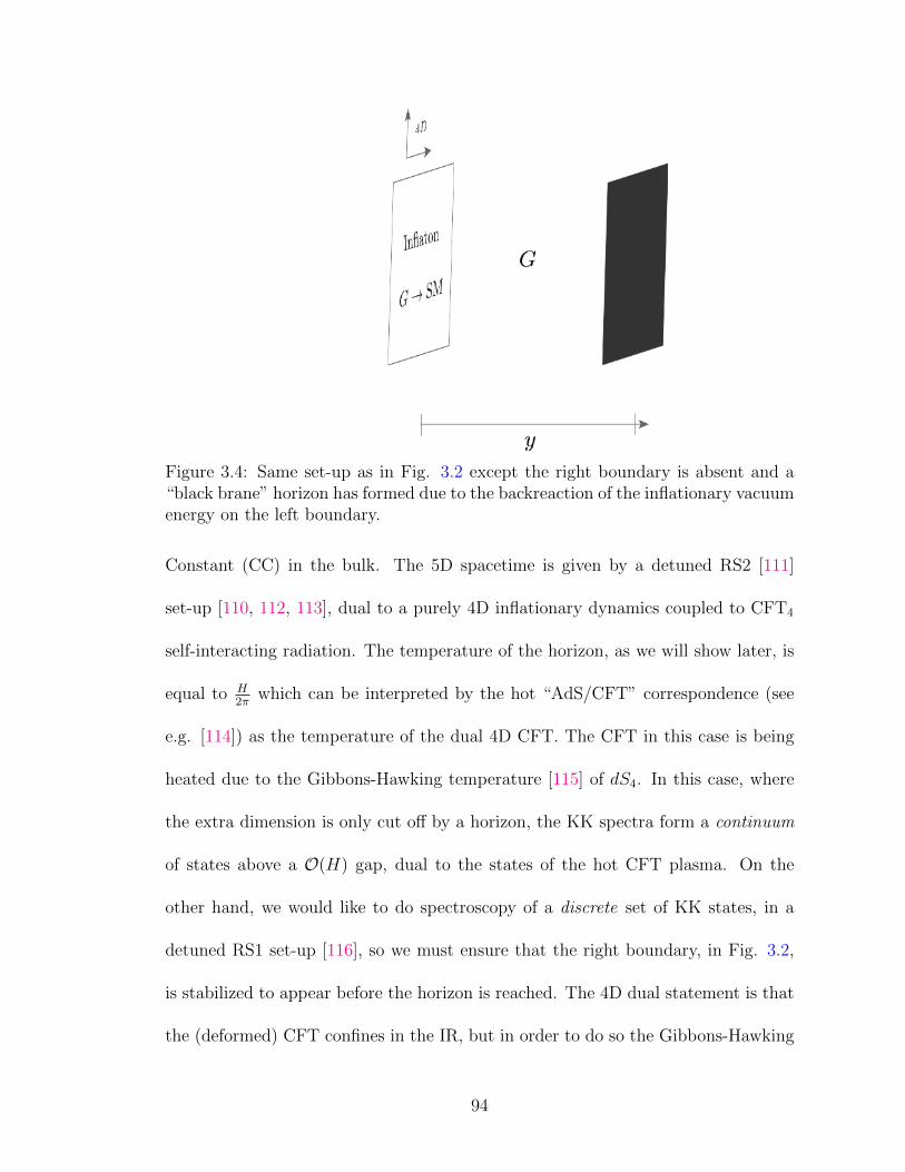
Figure 3.4: Same set-up as in Fig. 3.2 except the right boundary is absent and a“black brane” horizon has formed due to the backreaction of the inflationary vacuumenergy on the left boundary.

Constant (CC) in the bulk. The 5D spacetime is given by a detuned RS2 [111]

set-up [110, 112, 113], dual to a purely 4D inflationary dynamics coupled to CFT4

self-interacting radiation. The temperature of the horizon, as we will show later, is

equal to H2π

which can be interpreted by the hot “AdS/CFT” correspondence (see

e.g. [114]) as the temperature of the dual 4D CFT. The CFT in this case is being

heated due to the Gibbons-Hawking temperature [115] of dS4. In this case, where

the extra dimension is only cut off by a horizon, the KK spectra form a continuum

of states above a O(H) gap, dual to the states of the hot CFT plasma. On the

other hand, we would like to do spectroscopy of a discrete set of KK states, in a

detuned RS1 set-up [116], so we must ensure that the right boundary, in Fig. 3.2,

is stabilized to appear before the horizon is reached. The 4D dual statement is that

the (deformed) CFT confines in the IR, but in order to do so the Gibbons-Hawking

94

temperature must not exceed the deconfinement temperature. If this temperature

is exceeded, the (deformed) CFT is deconfined, dual to the horizon in 5D appearing

before the second boundary. We will find that there is a “window of opportunity”

for doing discrete spectroscopy using NG, constrained by the need for the de Sitter

temperature H/(2π) to be below the deconfinement temperature, but not so low

that cosmological production of the confined states (dual to discrete KK modes) is

Boltzmann suppressed. Studying this window will be a central part of our work. It

is complicated by the fact that in this regime there is a significant backreaction on

the Goldberger-Wise extra-dimensional stabilization mechanism [117] for the second

boundary due to the H-scale inflation. We perform a novel near-horizon analysis

in which this backreaction is systematically controllable. The final strength of NG

signals will also depend on the backreaction away from the near-horizon regime, but

only up to O(1) uncertainties, which do not affect their basic observability. We hope

to address these uncertainties in later work.

While the case of non-zero 5D CC offers a simple dual 4D interpretation, as

above, we will mostly focus on the case of vanishing 5D CC for technical simplicity.

However, the qualitative behavior is very similar to that with a CC, and the latter

continues to provide good intuition for our results. Although our focus in this

chapter will be on the orbifold GUTs scenario, our results related to KK gravitons

and stabilization of the extra dimension are quite general and will apply whenever

the size of the extra dimension is O(H−1).

This chapter is organized as follows. In Sec. 3.2 we detail the specific orbifold

set-up that we will be considering in this chapter and recall some aspects of the gauge

95

coupling unification in orbifold GUTs. In particular, we will see that with boundary

localized, non-GUT-symmetric 4D gauge kinetic terms one can easily fit the observed

values of gauge couplings. In Sec. 3.3 we will briefly review the NG signals mediated

by heavy particles. Sec. 3.4 focuses on various extra dimensional features of the

inflationary spacetime, as alluded to above, and ends with an estimation of the

strength of NG mediated by KK gravitons. Sec. 3.5 describes the inflationary

couplings of the KK gauge bosons of the GUT, listing all the higher dimensional

operators relevant for NG. We discuss the prospects of visibility when the GUT

group is either SU(5) or SO(10). Secs. 3.6 and 3.7 give the explicit form of NG

mediated by KK gravitons and KK gauge bosons respectively and calculate the

strengths of NG. We conclude in Sec. 3.8. Two technical appendices supplement

the discussion in the main text of the chapter. In Appendix B.1 we derive the

KK decomposition of the KK graviton-radion system, both reproducing some of the

existing results from the literature and establishing some new results that are used

in Sec. 3.4. In Appendix B.2 we derive the bispectrum mediated by KK gravitons

via a direct computation using the “in-in” formalism. This, as it should, reproduces

the form of [21] obtained via exploiting conformal symmetries of the late time slice.

Furthermore, our calculation also determines the overall normalization of the in-in

correlator.

96

3.2 Orbifold GUTs and Gauge Coupling Unification

3.2.1 Orbifold GUTs

We consider the simplest orbifold GUT structure with a 5D bulk, and with

a simple GUT gauge group such as SO(10) or SU(5). The 5D gauge theory is

necessarily a non-renormalizable effective field theory (EFT). The extra dimension

is physically an interval, although we will realize this as an S1/(Z2 × Z ′2) quotient

of a circle in order to precisely specify boundary conditions. While the 5D bulk

preserves the GUT gauge symmetry, it is broken on one of the boundaries of the

extra-dimensional interval (effectively Higgsed at the 5D EFT cutoff) down to just

the SM gauge group. We can think of this as effectively being given by imposing

Dirichlet boundary conditions (BC’s) on the broken gauge fields and Neumann BC’s

on the unbroken (SM) gauge fields on the GUT-breaking boundary, and all-Neumann

BC’s on the other GUT-symmetric boundary. Lastly, we will take the SM fermions

and the SM Higgs to be present in the bulk as well.

Before discussing gauge coupling unification in such a set-up, we give the

explicit extra dimensional profiles of the KK modes of the bulk gauge bosons given

our choice of BC’s. In this section we will assume a simple fixed 5D spacetime

product geometry consisting of 4D Minkowski spacetime and the extra-dimensional

interval. We will account for 5D curvature in later sections, but this will not change

the central structure of unification and its low-energy implications. For finding the

free-field profiles we can ignore the self-interactions of the bulk non-Abelian gauge

97

field.

Then the equation of motion (EOM) for each gauge field component is identical

to the Maxwell equations for a bulk U(1) gauge field. These are given by (suppressing

the adjoint index on the gauge field),

∂MFMN = 0. (3.2)

By a suitable gauge transformation we can go to the gauge where A5(x, y) = A5(x)

with y being the coordinate along the extra dimension. Furthermore, with our choice

of BC’s above, A5(x) = 0. Hence the Maxwell equations for Aν are given by,

∂νFνµ + ∂2yAµ = 0. (3.3)

Via a KK decomposition,

Aµ =∑l

Al,µ(x)ϑl(y), (3.4)

the 5D EOM (3.3) can be separated into a 4D EOM for a massive spin-1 particle

and an equation governing the extra dimensional profile,

∂νFl,νµ = m2lAl,µ, (3.5)

∂2yϑl +m2

l ϑl = 0. (3.6)

Here ml is the mass of the l-th KK mode. Using eq. (3.6) we can derive the profile

98

of SM and broken gauge fields (part of GUT/SM coset) for the above choice of BC’s,

ϑSMl (y) = cos(lπy/L), (3.7)

ϑGUT/SMl (y) = sin((l + 1/2)πy/L), (3.8)

with l being a non-negative integer. We have placed the boundaries at y = 0 and

y = L. Taking l = 0 we see that only the SM gauge bosons have a zero mode,

m = 0, whereas the lightest of GUT/SM bosons have a mass of m = π2L

and hence

no zero mode. This choice of BC’s has broken the GUT down to the SM at the

compactification scale, as expected.

3.2.2 Gauge Coupling Unification

The action for the gauge sector is given by,

S ⊃∫d4x

∫ L

0

dy√−G

(1

g25

FMNFMN + δ(y)

∑i

κiFi,µνFµνi

), (3.9)

where M,N and µ, ν run over the 5D and 4D indices respectively. The first term

describes the field strength for the bulk GUT gauge theory. For generality, we

have also included boundary localized, non-GUT-symmetric 4D gauge kinetic terms,

where the label “i = 1, 2, 3” denotes the U(1), SU(2) and SU(3) SM subgroups. We

can now relate the gauge couplings g4,i1 in the 4D low energy effective theory with

the 5D gauge coupling g5. To this end, we note that the zero modes of the gauge

1Here we are making a small change in notation compared to Fig. 3.1 by making the replacementgi → g4,i for i = 1, 2, 3.

99

bosons have a flat profile, as seen from eq. (3.7) for l = 0, in the extra dimension.

Then using the Lagrangian (3.9) and doing an integration over the extra dimension

we get the relation between the SM gauge couplings at the compactification scale

(see e.g. [85]),

α−1i

(1

L

)≡ 4π

g24,i

=4πL

g25

+ 4πκi. (3.10)

Below the unification scale mKK ∼ 1/L, the couplings g4,i evolve as per the usual

SM RGE which at 1-loop reads as,

α−1i (µ) =

4πL

g25

+bi2π

log

(mKK

µ

)+ 4πκi. (3.11)

In the above bi = (4110,−19

6,−7) are the three 1-loop SM beta functions with the nota-

tion that g4,1 =√

5/3g′ where g′ is the SM hypercharge coupling. This has precisely

the one-loop form of a traditional 4D GUT, if we translate αGUT = g25/4πL,MGUT =

mKK and the κi are interpreted as GUT threshold corrections. We see that for suf-

ficiently large L and sufficiently long running, the first two terms on the right dom-

inate, with the “threshold corrections” κi giving a subleading contribution. This

structure then predicts that plotting 1/αi(µ) vs. log µ will give three lines almost

meeting at a point, as indeed the data suggests in Fig. 3.1.2 As a benchmark choice

taking, κ1 = 4016π2 , κ2 = 60

16π2 and κ3 = 116π2 we can describe the observed gauge cou-

plings at the weak scale and achieve unification in the sense described above with,

2The minimal radiatively stable size of the κi is ∼ 116π2 . But it is perfectly natural for the the

κi to take larger values, required to interpret Fig. 3.1 in the orbifold GUT scenario as we do here.

100

α−1G = 39, mKK = 5× 1013GeV. (3.12)

The lower unification scale of non-supersymmetric GUTs∼ 1014 GeV raises the

danger of an unacceptably large proton decay rate mediated by GUT states. In orb-

ifold GUTs this is straightforwardly avoided by the mechanism of “split multiplets”

whereby SM quarks and leptons are housed within different GUT multiplets, so

that baryon and lepton number can be separately assigned, and unwanted fermionic

zero-modes in these multiplets are removed by Dirichlet BC’s on the GUT-breaking

boundary [86].

3.3 Non-gaussianity and Massive Particles

In this section we briefly review NG signals arising from massive particles

during inflation. For a more thorough explanation of how cosmological correlation

functions are defined and the formalism used to calculate them, the reader is referred

to chapter 2, along with the literature [32, 63]. Inflaton self-interactions or presence

of other light fields with masses H, can contribute to primordial NG. However,

a very distinctive non-Gaussian feature of primordial fluctuations can emerge, if

massive fields with m ∼ H are produced during inflation with sufficiently strong

coupling to the inflaton, in the “squeezed” limit when one of the inflaton momenta

becomes much smaller than the others (say, k3 k1 ∼ k2). Depending on the

mass (m) and spin (s) of such a particle, the bispectrum mediated by it will have a

101

non-analytic momentum dependent part of the form [18, 19, 20, 21, 36, 37, 40],

F nonanalytics=0 ∝ f0(µ0)

(k3k1

) 32

+iµ0+ f0(−µ0)

(k3k1

) 32−iµ0

, (3.13)

F nonanalytics=1 ∝ sin2 θ ×

(f1(µ1)

(k3k1

) 52

+iµ1+ f1(−µ1)

(k3k1

) 52−iµ1

), (3.14)

F nonanalytics=2 ∝

(cos2 θ − 1

3

)×(f2(µ2)

(k3k1

) 32

+iµ2+ f2(−µ2)

(k3k1

) 32−iµ2

). (3.15)

In the above, µ0 = µ2 =√

m2

H2 − 94

and µ1 =√

m2

H2 − 14

are given in terms of the

mass m of the massive particle. The spin dependence is encoded in the prefactors

with θ = k1 · k3. The non-analytic dependence on momenta also follows from simple

considerations as reviewed in chapter 2. The functions fs(µs) can be calculated

given the coupling between inflaton and the massive particle. For the detailed form

of fs(µs) see e.g. [18, 19, 20, 21, 24, 36, 37, 40, 78] for spin-0; [24] for spin-1; eq.

(169) of the present thesis and [21, 40, 91] for spin-2. While the Hubble spacetime

expansion can readily produce particles with masses of order H or smaller, for

larger masses there is a “Boltzmann suppressed” production amplitude, generically

fs(µs) ∼ e−πµs ∼ e−πm/H for m H. While extra dimensions certainly give rise to

higher spin particles such as our KK gravitons, with a lower bound on their masses to

avoid horizon formation, there is an even more robust bound on higher spin masses

in 4D dS spacetime regardless of their origin. For spin-2 this is given by the Higuchi

bound, [118]. We will show that horizon non-formation is a stronger condition in

the extra dimensional scenario so that the Higuchi bound is automatically satisfied.

Importantly, the non-analytic momentum dependence shown above cannot be

“faked” by inflaton self-interactions since the NG contribution of the latter have

102

only an analytic momentum dependence in the squeezed limit—making the non-

analyticity a “smoking gun” signal of new particles during inflation [21].

3.4 Inflation and the Fifth Dimension

3.4.1 General Set-up

We consider a 5D spacetime in which the extra dimension is an interval and

localize a 4D inflaton on one of the boundaries at an end of the interval. Technically,

we will realize this interval as an S1/(Z2 ×Z ′2) orbifold in order to determine BC’s.

Set-ups with boundary localized inflaton have been considered in the literature, see

e.g. [109, 110, 112, 113, 119, 120, 121, 122]. We will see that for sufficiently large H

the non-inflaton boundary can become shrouded by a black brane horizon, effectively

leaving a set-up with a single boundary. To most simply explore this, we will also

consider the limiting case of semi-infinite extra dimension.

The 5D action has the basic structure,

S =

∫d4x

∫ L

0

dy√−G(2M3

5R5 − Λ5)−∫d4x

∫ L

0

dy√−Gδ(y)V0

+

∫d4x

∫ L

0

dy√−G

(−δ(y − L)VL +

(−1

2GMN∂MΣ∂NΣ− V (Σ)

)),

(3.16)

where the bulk metric is denoted by GMN and G = det(GMN). R5 is the 5D

Ricci scalar. Here we have placed the boundaries at y = 0 and y = L where y is

the coordinate along the extra dimension. There are boundary-localized potentials

103

V0, VL at y = 0 and y = L respectively. M5 is the 5D Planck scale whereas Λ5 is the

5D cosmological constant. We take the inflaton field to live at y = 0, but begin by

neglecting its rolling, so that its potential is a approximately constant V0 ∼M24H

2,

where M4 is the final effective 4D Planck scale. We will however consider VL to

be an exactly constant “brane tension”. We also have a bulk 5D Goldberger-Wise

(GW) scalar Σ [117] with a potential V (Σ) that stabilizes the extra dimension. The

case with a single boundary will be realized by taking L→∞ limit.

Requiring a dS4 foliation (in the limit of no-rolling of the inflaton) and a static

extra dimension we are lead to the ansatz,

ds2 = −n(y)2dt2 + n(y)2a(t)2d~x2 + dy2, (3.17)

where a(t) = eHt is the scale factor, and n(y) is the warp factor. In the presence of

dS4 isometry, only the 00 and 55 Einstein equations are independent,

H2 − n(y)n′′(y)− n′(y)2 =1

4M35

n(y)2

3

(1

2Σ′(y)2 + V (Σ) + Λ5

), (3.18)

n′(y)2 −H2 =1

4M35

n2(y)

6

(1

2Σ′(y)2 − V (Σ)− Λ5

). (3.19)

Here and in the rest of the chapter the ′ will always denote a derivative with respect

to the explicitly mentioned argument of the function. For example, n′(y) and n′(z)

will denote dn(y)dy

and dn(z)dz

respectively. The Einstein equations above have to be

104

supplemented with BC’s 3,

limε→0

[n′(y)

n(y)

]+ε

−ε= − V0

12M35

, (3.20)

limε→0

[n′(y)

n(y)

]L+ε

L−ε= − VL

12M35

. (3.21)

3.4.1.1 Gravitational Fluctuations

The inflationary dS4 foliation necessarily “warps” the extra dimension, even

when there is no bulk energy-momentum tensor. Thus the KK spectrum is also

expected to be different from the non-inflationary 4D Lorentz-invariant case, with

Mink4 foliation. General gravitational fluctuations around the metric (3.17), con-

tains the graviton hµν(x, y) and, in presence of the second boundary, the radion

Π(x, y). We will show in Appendix B.1 that the linearized equation of motion for

the spin-2 graviton and spin-0 radion decouple for a general warp factor n(y). Thus

postponing the discussion of radion to a later subsection, we focus only on the 4D

graviton and its KK modes for now. These fluctuations can be parametrized at the

linearized level as,

ds2 = −n(y)2dt2 + n(y)2a(t)2d~x2 + dy2 + hµν(x, y)dxµdxν , (3.22)

3We are considering the extra dimension to be a S1/(Z2 × Z ′2) orbifold which gives rise to the

BC’s mentioned here.

105

where µ, ν denote 4D indices t, ~x. In the above we have chosen h5µ = 0 by a suitable

gauge transformation, and hµν satisfies transverse and traceless conditions,

∇µhµν = 0; hµµ = 0. (3.23)

The equation of motion for the graviton can be obtained as [123, 124, 125] (for a

derivation see Appendix B.1)

dShµν(x, y) +(n2(y)∂2

y − 2n′(y)2 − 2n(y)n′′(y)− 2H2)hµν(x, y) = 0, (3.24)

where dS = gµν∇µ∇ν is the laplacian operator for dS4 with gµν is the metric for

dS4 i.e. ds24D = gµνdxµdxν = −dt2 + a2(t)d~x2. To make the KK decomposition

manifest we can redefine hµν = n2hµν to get

dShµν(x, y) +n2(y)∂2y hµν(x, y) + 4n(y)n′(y)∂yhµν(x, y)−2H2hµν(x, y) = 0. (3.25)

Expanding hµν into KK modes hl,µν(x) with profile χl(y)

hµν(x, y) =∑l

hl,µν(x)χl(y), (3.26)

we get

dShl,µν(x) = (m2 + 2H2)hl,µν(x) (3.27)

n2(y)χ′′l (y) + 4n(y)n′(y)χ′l(y) +m2χl(y) = 0. (3.28)

106

These describe hl,µν as spin-2 particles with mass m in dS4. The form taken by the

bulk profile is most clear in the analog 1D “quantum mechanics” coordinate system,

where eq. (3.28) has the same form as Schroedinger equation with some potential

determined by the warp factor n(y) [111]. To achieve this, we can do a variable

change n(y) ddy

= ddz

and a field redefinition

χl(z) = n−32 (z)ψl(z) (3.29)

to get,

−1

2

d2

dz2ψl(z) +

(3

8

(n′(z)

n(z)

)2

+3

4

n′′(z)

n(z)

)ψl(z) =

m2

2ψl(z). (3.30)

We note that the effect of the bulk scalar Σ comes only through the dependence on

the warp factor n(y) given via eqs. (3.18) and (3.19). This is because the spin-0

fluctuations of Σ cannot mix with spin-2 hµν at the linearized level. The zero mode

profile for m = 0 in eq. (3.30) can be obtained for a general warp factor n(z) with

ψ0(z) ∝ n32 (z).

3.4.2 Semi-Infinite Extra Dimension

We now specialize to the case in which there is only one boundary at y =

0, housing the inflaton. In this case, the radion is no longer in the spectrum.

We therefore drop the stabilizing GW fields, and for simplicity consider vanishing

5D bulk cosmological constant. Then the warp factor n(y) satisfying eqs. (3.18),

(3.19) and KK graviton profile obeying eq. (3.30) simplifies significantly as we now

107

demonstrate.

3.4.2.1 Background Solution and the Horizon

The solution to eq. (3.18) and eq. (3.19) along with BC eq. (3.20) and

normalization n(y = 0) = 1 is then given by

n = 1−Hy, (3.31)

with V0 = 24M35H > 0. We see that the presence of the inflationary vacuum energy,

characterized by H 6= 0, has “warped” the extra dimension giving rise to a horizon

at y = H−1 [109, 110].

Horizon Temperature. The temperature of the horizon can be found by studying

the near horizon geometry. A variable change Y = H−1 − y shows that the line

element transverse to the boundary becomes identical to a Rindler metric,

ds2 = −H2Y2dt2 + dY2. (3.32)

The temperature of this Rindler horizon can be found by the standard method of

going to Euclidean time and demanding regularity of the metric at the horizon,

Thorizon =H

2π. (3.33)

108

This is same as the Gibbons-Hawking temperature of dS4 space [115]. At first, this

coincidence of these temperatures is not clear.

We gain insight by considering the case with negative 5D cosmological constant

Λ5 = −24M35k

2 in the bulk, which corresponds to the RS2 set-up [111], but with

de-tuned boundary tension giving rise to dS4 foliation rather than Mink4 foliation.

The bulk equations (3.18) and (3.19) can again be solved [110, 112, 113],

n(y) = cosh(ky)−√H2 + k2

ksinh(ky). (3.34)

With this warp factor, we again see the presence of a horizon with an identical

near horizon geometry as before and horizon temperature Thorizon = H2π

. This can

be interpreted as the temperature of the 4D CFT dual to RS2, as follows from

the “hot” AdS/CFT correspondence. The CFT in this case is being heated by the

dS4 Gibbons-Hawking temperature due to 4D inflation. For aspects of such “hot”

AdS/CFT correspondence, see [114] and references therein.

3.4.2.2 KK Graviton Wavefunction

For now, let us return to the technically simpler case with vanishing Λ5 (at the

loss of holographic insight). Using the explicit form of the warp factor eq. (3.31) in

eq. (3.30) we obtain

d2

dz2ψl(z) + (m2 − 9

4H2 +

V0

8M35

δ(z))ψl(z) = 0, (3.35)

109

where the coordinate z is defined by e−zH = 1 −Hy 4. Thus the horizon has been

pushed to z =∞, whereas the y = 0 boundary resides at z = 0.

Remarkably, there is a m = 0 normalizable and localized graviton mode,

ψ0(z) ∝ e−32Hz, (3.36)

corresponding to a finite 4D effective Planck scale, M4, as we will detail later. This

is similar to the RS2 graviton localization giving an effective 4D gravity despite the

infinite extra dimension, but here the localization relies on 4D inflation, H 6= 0.

Intuitively, the horizon provides a second boundary cutting off the infinite extra

dimension. We also see that for m 6= 0 there is a mass gap of 3H/2 and a continuum

of modes for m > 3H/2. These modes are non-normalizable and their profile in the

extra dimension is sinusoidal. This mass gap aligns nicely with the fact that a

massive spin-2 particle in dS4 has to obey the Higuchi bound [118] m2 ≥ 2H2,

which can be derived just by unitarity of the 4D theory. (In inflationary scenarios

where the dS4 isometries are significantly broken, the Higuchi bound can be evaded

and it is consistent to have spin-2 particles with m2 < 2H2 [126].) It should be

mentioned that for Λ5 < 0, some of these features persist and have been pointed

out in the literature, for e.g. [123, 124, 125].

In this chapter we will be interested in inflaton NG mediated by massive

particles (with or without spin) having a discrete spectrum. Hence to discretize the

continuum modes with m > 3H2

above, we need to reintroduce a second boundary

4The delta function δ(z) originates because of the R1/Z2 quotient of an infinite extra dimensionto obtain a semi-infinite extra dimension in the present case.

110

before the horizon is reached at y = H−1. We turn to this next.

3.4.3 Introduction of the Second Boundary

When the second boundary is introduced, the KK graviton wave function

ψl(z) has to obey two BC’s so that the KK continuum above becomes discretized.

Furthermore the radion is a physical degree of freedom and we have to stabilize it.

3.4.3.1 Radion Mass and Stabilization

We first set Λ5 = 0 and ask what happens in the absence of a GW field.

Using the metric solution, subject to dS4 ansatz, given in eq. (3.31), and the jump

equations (3.20) and (3.21) the radius of the extra dimension is determined

L =VL + V0

VLH, (3.37)

even in the absence a GW field. Note that we need to have VL < 0 for there to

be no horizon formed between the two boundaries. However, this dS4-symmetric

configuration is unstable as we discuss now.

We can parametrize the linearized radion fluctuation as [127]

ds2 = −n(y)2(1− 2Π(x, y))dt2 + n(y)2a(t)2(1− 2Π(x, y))d~x2 + (1 + 2Ξ(x, y))dy2.

(3.38)

Although we have two seemingly independent functions, Π(x, y) and Ξ(x, y) to de-

note the radion, the perturbed 0i Einstein equations force Ξ(x, y) = 2Π(x, y) [127].

111

Then the perturbed 55 Einstein equation, along with the background solution, gives

the linearized radion equation of motion (for a derivation see Appendix B.1),

dSΠ + 4H2Π = 0. (3.39)

We see that the radion has a tachyonic mass m2r = −4H2, signalling instability [128].

For the case of Λ5 < 0, it is still true thatm2r = −4H2 [129, 130, 131]. Although

this can again be deduced by considering the perturbed Einstein equations, we can

get the same result from a “simple” holographic insight. To this end we calculate

the radius of the extra dimension via a similar procedure as above. Using eq. (3.34)

and eqs. (3.20), (3.21) we get,

tanh(kL) =V0 + VL

24M35k + V0VL

24M35 k

. (3.40)

To have a solution to the above equation we need VL < −24M35k. Now let us write

down an effective potential for the canonically normalized radion field Πc (which is

proportional to Π) on this dS4 symmetric background. As the Goldstone boson of

spontaneous conformal symmetry breaking of the CFT dual to the bulk dynamics,

the only possible conformally invariant form of the radion potential is,

Vr(Πc) = H2Π2c + λΠ4

c . (3.41)

A conformal coupling of the radion to the 4D Ricci scalar, L ⊃ − 112RΠ2

c + · · · fixes

the mass term above with R = 12H2 for dS4. A quartic coupling λ is also expected

112

to be present whenever the tension on the second boundary VL is not equal to the

tuned RS1 value of −24M35k, with sgn(λ) being fixed by sgn(VL + 24M3

5k) (see e.g.

[132]). Since we needed VL < −24M35k in the present case, we have λ < 0. If we

now expand around the correct minima of Πc, we get back the identical tachyonic

mass m2r = −4H2 as before.

The tachyonic radion necessitates the presence of some stabilization mecha-

nism. Since the tachyonic instability is ∼ −O(H2) and we are interested in having

mKK ∼ H for observability of NG, the stabilization will necessarily have an O(1)

backreaction on the geometry. However, this makes the analysis technically more

difficult since we have to solve coupled field equations for the GW field and the

metric. Fortunately, as we discuss below, this analysis simplifies in a near-horizon

approximation and yields important qualitative insights.

3.4.3.2 Near-horizon Analysis of Stabilization

We begin by noting that the observability of KK gravitons of the compactified

(2-boundary) scenario is tightly constrained by purely 4D considerations: Boltz-

mann suppression ∼ e−πµ for large m and the Higuchi lower bound m >√

2H

(following from unitarity). The former can be seen by an explicit calculation of the

bispectrum due to KK graviton exchange which we carry out in Appendix B.2 and

detail further in Section 3.6. In Fig. 3.5 we plot the function f2(µ) (defined in eq.

(3.90)) which characterizes the strength of NG due to KK graviton exchange and

from there it is evident that significant Boltzmann suppression kicks in soon as m

113

gets bigger than 3H2

5. Hence to have an observable NG mediated by KK gravitons,

we need to have their masses within a narrow window about 3H2

.

Fortunately, we saw above that in the absence of a second boundary, there is a

horizon at a finite proper distance y = H−1 and a continuum of KK graviton modes

starting precisely at 3H2

. In the presence of a second boundary this continuum spec-

trum must turn into a discrete one. However if the warp factor n(y) on the second

boundary is 1, i.e. if the second boundary is placed just in front of a “would-be”

horizon, we expect to get back a finely discretized spectrum of KK gravitons starting

around m = 3H/2, thereby avoiding significant Boltzmann suppression. To show

this we first write the linearized warp factor near the second boundary as,

n(ε) ≈ Hε, (3.42)

where ε is the coordinate along the extra dimension and the horizon is reached as

ε → 0 6. Again with the coordinate transformation −n ddε

= ddz

we can write the

equation of motion for the wave function in the analog 1D “quantum mechanics”

coordinate system, as in eq. (3.30),

−ψ′′l (z) + (9H2

4−m2)ψl(z) = 0. (3.43)

This form is identical to what we had in the absence of the second boundary, eq.

5The apparent divergence of |f2(µ)| as µ→ 0 is actually absent in the full bispectrum, since inthe limit of µ→ 0 only the real part of f2(µ) contributes which remains finite.

6ε can be related to y once we know the warpfactor along the entire extra dimension, but inthis chapter we will be solving for the warp factor only near the second boundary.

114

(3.35), without the delta function source 7. However, unlike that case, now the z

coordinate does not extend to ∞, but rather to some finite, but large (in units of

1/H) value. Since n(ε) ≈ e−zH , by making the warp factor on the second boundary

smaller, we can make the size of the “box” bigger in the analog quantum mechanics

problem, and thereby decreasing the spacing between the KK modes.

Having motivated the need for a near-horizon boundary, we now have to ask

whether such a configuration can actually be stabilized. To this end, we reintroduce

a GW field Σ with a bulk mass mΣ. Then its extra dimensional profile follows the

bulk equation of motion with dS4 ansatz,

Σ′′(y) + 4n′(y)/n(y)Σ′(y) = m2ΣΣ(y). (3.44)

We have to solve the coupled set of equations (3.18), (3.19) and (3.44) to obtain

a consistent background solution, which is difficult to do in general. But in the

near-horizon limit we are interested in we can solve the coupled set of equations

perturbatively in Hε. We take the ansatz for the warp factor and the profile to be

n(ε) = a1Hε+ a2H2ε2/2 + a3H

3ε3/3 + · · · (3.45)

Σ(ε) = b0 + b1Hε+ b2H2ε2/2 + b3H

3ε3/3 + · · · . (3.46)

We will focus on the regime H−1 ε > εc with εc being the location of the second

7Note that by a slight abuse of notation we used the same variable z in both eqs. (3.35) and(3.43) whereas they match only very near the horizon

115

boundary. The solution to eqs. (3.18),(3.19) and (3.44) is given by,

n(ε) = Hε− 1

72v2m2

ΣHε3 + · · · (3.47)

Σ(ε) =√

4M35

(v +

1

10vm2

Σε2 + · · ·

), (3.48)

where v is some constant fixed by the BC’s on the GW field. Note when the

stabilizer is absent i.e. v = 0, we get back the near horizon behavior given in (3.31)

with ε = H−1 − y.

Now let us analyze the radion equation of motion. For this we have to consider

the fluctuation σ(x, y) of the background GW field Σ(y), since the former can mix

with the radion. We can go through the perturbed Einstein equations once again

to get the equation of motion for the radion (144),

1

n2dSΠ = −Π′′−2n′Π′/n+4((

n′

n)2− n

′′

n)Π+2

Σ′′

Σ′(Π′+2n′Π/n)−6H2Π/n2. (3.49)

In the above, we have used the bulk equation,

Π′ + 2n′

nΠ =

1

12M35

σΣ′, (3.50)

to eliminate σ dependence in eq. (3.49). We have also used ′ to denote ∂∂y

. We can

now plug in the background solutions given by eqs. (3.47) and (3.48) in eq. (3.49)

to find,

Π(x, ε) ∝ (Hε)12±ν + · · · (3.51)

116

with ν =√

94− m2

r

H2 . In the absence of the GW field we had to have m2r = −4H2

to satisfy the radion equation of motion (3.39). Now, with the stabilizer such a

constraint has disappeared since eq. (3.51) is a near-horizon solution for arbitrary

mr, and with a suitable choice of BC’s we can make m2r > 0. Thus by studying the

near horizon geometry, we have shown how to stabilize the radion in presence of a

GW field.

We see that we can stabilize the second boundary arbitrarily close to the would-

be horizon, and that this results in a finely-spaced spin-2 KK spectrum beginning

arbitrarily close to m = 3H/2. This demonstrates that the KK modes need not

suffer large Boltzmann suppressions in their NG contributions.

Before proceeding further, let us make a comment about the KK spectrum

during and after inflation which we denote by M infKK and M today

KK respectively. We

should note that the observed values of the SM gauge couplings suggest, within the

orbifold GUT paradigm, an extra dimension with size M todayKK ∼ 1014 GeV today.

On the other hand, an inflationary Hubble scale Hinf ∼ 5× 1013 GeV is allowed by

data and motivated by high-scale inflation models. Thus we see that it is entirely

possible to have M todayKK ∼ Hinf. But this alone does not guarantee that we will see

interesting and observable NG signals due to KK states, since for that we actually

need M infKK ∼ Hinf. Here is where the stabilizing GW scalar plays a crucial role by

determining the size of the extra dimension, in the low curvature regime given by

M todayKK ∼

Htoday≈0mΣ ln(v1/v2), (3.52)

117

where the v1,2 are the VEVs of the GW scalar on the two boundaries. Since we

are considering M todayKK ∼ 1014 GeV today, this implies mΣ ∼ 1014GeV ∼ Hinf.

With mΣ ∼ Hinf, our near-horizon analysis then shows that there is no obstruction

in stabilizing the non-inflaton boundary near the would-be horizon, guaranteeing

M infKK ≈ 3Hinf/2. We can contrast this with what would have happened if either

M todayKK Hinf or M today

KK Hinf. In the former case, we would have mΣ Hinf, and

Hubble expansion would generically8 be subdominant in the stabilization dynamics

from the time of inflation all the way until today, so that M infKK ≈ M today

KK Hinf,

and seeing the GUT states would be highly Boltzmann suppressed. In the latter

case, we would have mΣ Hinf, and the σ mixing terms in eq. (3.50) would be

negligible, so we would approximately have the unstabilized result that the radion

would be tachyonic if the boundary is near the horizon. Thus, the rough coincidence

M todayKK ∼ Hinf plays a critical role in allowing us to see the GUT states in NG.

3.4.4 Inflationary Couplings

3.4.4.1 Wavefunction of KK Graviton on Inflationary Boundary

To determine the coupling of the KK graviton to the inflaton, localized at

the y = 0 boundary, we will need the wavefunction of the KK graviton at y = 0.

However, we have argued above that to stabilize the radion, the backreaction of

the GW field on the metric will typically be O(1), so that this will also affect the

8We can see this in eqs. (3.47) and (3.48), where the near-horizon expansion for large mΣ Hclearly requires parametrically small εc, which in turn requires εc-level tuning of parameters tostabilize. Generically there is no such tuning and hence no near-horizon stabilization for mΣ H.

118

KK graviton wavefunction at the O(1) level. In order to precisely calculate this we

would have to extend our near-horizon analysis of the last subsection to the entire

extra-dimensional interval. It would be interesting to find some analytic means of

doing this (non-perturbative in H) , but as yet we do not have such an analysis.

The superpotential approach taken in [133] may be useful in this regard. Here, we

will simply estimate the KK graviton wavefunctions by ignoring the backreaction

completely, but assign an O(1) uncertainty to this estimate.

We therefore proceed by beginning with the metric for the single boundary

set-up, eq. (3.31), but taking the extra dimension to simply be cut off by the

location of the second boundary at say yc before reaching the horizon. This neglects

the backreaction of the requisite stabilization of the second boundary, as discussed

above. In terms of the coordinate z defined by n ddy

= ddz

, we have n(z) = e−zH with

the extra dimension ranging from z = 0 to zc = − 1H

ln(1 − Hyc). Furthermore in

this coordinate system the profile of KK modes, obeying eq. (3.35), is sinusoidal.

The orthonormality condition is given by

2M35

∫ zc

0

dzψ∗l (z)ψm(z) =M2

4

2δlm, (3.53)

where the numerical factor is chosen to ensure that the 4D action is given by

M24

2

∫d4xR4 with R4 and M4 being the 4D Ricci scalar and the 4D Planck scale

respectively. As will be explained below M4 differs from the standard Planck scale

Mpl = 2.4×1018 GeV by some O(1) amount due to inflationary dynamics. However

in the end, this difference will not be important for us because the final strength of

119

KK graviton NG (3.90) will be dependent on M4 only via the tensor-to-scalar ratio

r. Thus only the observational upper bound on r [8], rather than an actual knowl-

edge of M4, will be important. Thus in the z coordinate system, the wavefunction

behaves as if it is in a flat extra dimension and after normalization, it will carry

the usual “ 1√Volume

dilution factor” (see e.g. [134]). On the boundary containing the

inflaton, the wavefunction is given by,

ψl(z = 0) ∼ 1√Hzc

∼ 1√− ln(n(yc))

(3.54)

with zc being the “volume” of the extra dimension. In the above, we have used the

relation zc = − 1H

ln(1 − Hyc) = − 1H

ln(n(yc)). As we show in the following, the

strength of the coupling between the inflaton and the KK graviton is proportional

to ψl(z = 0) and eq. (3.54) shows that such a coupling is only logarithmically sup-

pressed when we place the second boundary very near a would-be horizon. Crucially,

this will allow us to get an observable NG signal mediated by KK gravitons, without

paying a large wavefunction suppression in the coupling strength. This logarithmic

suppression, however, seems unavoidable in our set up. This is because, although

decreasing the size of the extra dimension will increase the overlap between the in-

flaton and the KK graviton—hence increasing the coupling—it is also expected to

make the KK gravitons heavier and thereby we will incur exponential Boltzmann

suppression in NG signals. Let us now write down the explicit inflaton-KK graviton

coupling using which we estimate the strength of NG mediated by KK gravitons in

the subsequent discussion.

120

3.4.4.2 Coupling of KK Graviton to the Inflaton

At the linear order, the graviton fluctuations couple to the energy-momentum

tensor of the inflaton in the standard way, namely,

Sint =

∫d4x

δSinfδgµν

hµν = −1

2

∫d4x√−gT µνinfhµν (3.55)

where we have used the definition of the energy momentum tensor T µνinf = − 2√−g

δSinfδgµν

.

Since we are using the convention that the warp factor n(y = 0) = 1 on the infla-

tionary boundary, using the expansion (3.26) and eq. (3.29) we can simplify eq.

(3.55) as,

−1

2

∞∑l=0

∫d4x√−gT µνinf hl,µνψl(0). (3.56)

Upon canonically normalizing 9 the massless 4D graviton and the KK modes, from

the above we get,

− 1

M4

∫d4x√−gT µνinf (h0,µν + h1,µνψ1(0) + · · · ) (3.57)

We have set ψ0(0) = 1 without loss of generality and focused only on the first (i.e.

the lightest) KK mode for concreteness. Finally using the fact that we are in the

gauge hµµ = 0 we get the coupling between the inflaton and the KK graviton,

− 1

M4

∫d4x√−g∂µφ∂νφ(h1,µνψ1(0) + · · · ). (3.58)

9We will continue to denote the canonically normalized KK gravitons by the same variable hl,µνto simplify the notation.

121

3.4.4.3 Estimate of NG Mediated by KK Graviton

Let us now give a quick estimate of the NG mediated by KK graviton using

the coupling in eq. (3.58). We can expand the inflaton in terms of the background

φ0 and the fluctuation ξ to get,

−ψ1(0)

M4

hµν1 ∂µφ∂νφ = −ψ1(0)

M4

hµν1 (∂µφ0∂νφ0 + 2∂µφ0∂νξ + ∂µξ∂νξ) (3.59)

The first term gives a small tadpole, which can be shifted via a field redefinition

without affecting the relevant couplings significantly, whereas the second term after

using ∇µhµν = 0 gives,

−2ψ1(0)

M4

Hφ0ξh001 . (3.60)

Hence the relevant couplings are given by,

−2ψ1(0)

M4

Hφ0ξh001 −

ψ1(0)

M4

hµν1 ∂µξ∂νξ. (3.61)

From the above we can get a quick estimate of the parametric strength of NG defined

in eq. (4.6),

F ∼ ψ1(0)

M4

× ψ1(0)φ0

M4

× φ0

H2∼ φ2

0

M24H

2× ψ1(0)2, (3.62)

while a detailed form containing the momentum dependence as in eq. (3.15) will be

given in Sec. 3.6.

The quantityφ20

M24H

2 differs by an O(1) factor from its standard value of 2ε in

a purely 4D set-up [121] where ε ≡ − HH2 . To understand why, note that ordinarily

122

after compactification, the 4D EFT is generally an expansion in E/mKK < 1. In

cosmology a characteristic energy scale is E ∼ H, and in the present context we

seek mKK comparable to H for KK visibility in NG. Therefore we should expect

O(1) corrections relative to the leading 4D predictions. To see this explicitly we can

consider the inflaton EOM with the potential V0 (which we previously approximated

as a constant) on the inflationary boundary,

φ0 + 3Hφ0 +dV0

dφ= 0. (3.63)

The Friedman equation, following from eq. (3.20) (with the warp factor n(y) =

1−Hy) reads as,

1

2φ2

0 + V0 = 24M35H. (3.64)

Using the relation (3.67) between M5,M4 and H, M24 = 4M3

5L(

1−HL+ H2L2

3

),

and using the usual definition of ε = − HH2 , one sees that

φ20M2

4H2 6= 2ε.

It will be useful to write the quantityφ20

M24H

2 in terms of the tensor to scalar

ratio, r, in order to estimate the strength of the KK graviton mediated NG signals

in Sec. 3.6. In our set-up, the scalar power spectrum will be unaffected, to the

leading order in slow-roll parameters, by the presence of the extra dimension since

the inflaton fluctuations are localized on the boundary [120, 121]. Hence r is given

by,

r ≡ PT,kPS,k

= 8φ2

0

H2M24

. (3.65)

In the above, we have used the tensor power spectrum, PT,k = H2

M24

4k3

, and the scalar

123

power spectrum PS,k = H4

φ20

12k3

.

Now we come back to the estimate of F in eq. (3.62). As argued earlier, the

wavefunction suppression above is quite mild and hence the KK graviton mediated

NG is expected to be of the order of fNL ∼ r < 10−1. While inaccessible by future

large-scale structure surveys [9], such a level of NG should be potentially observable

by 21-cm experiments probing the dark ages [11] if we have a high scale inflation

scenario with H . 1013 GeV. We conclude this section by checking whether such a

large value of H is consistent within our set-up.

Cutoff of 5D Gravity. To have quantum gravity corrections under control, we

should have V0 < M45 . To check that, first we recall the graviton zero mode profile

given in eq. (3.36),

ψ0 = e−3H2z, (3.66)

and use the normalization condition in eq. (3.53) to get,

M24 = 4M3

5L

(1−HL+

H2L2

3

)(3.67)

In the above we have assumed the warp factor is given by n(y) = 1 −Hy ignoring

the backreaction of the stabilizer field. Taking L ≈ 1/H we get,

V0

M45

= 24(4/3)1/3 × (H/M4)2/3 1. (3.68)

124

3.5 Gauge Theory States

Whereas observing a KK graviton resonance via NG would be striking, it

would be even more so if we see the accompanying signatures of massive gauge

bosons. The latter can arise naturally in our set up as the KK modes of the bulk

unified gauge fields. The observability of NG mediated by such KK gauge bosons

will depend both on their masses and coupling to the inflaton. Interestingly, we

will see below that the set-up with a near-horizon second boundary, chosen above

to give us mgravitonKK ∼ O(H), also yields mgauge

KK ∼ O(H). Thus in such a set-up, the

cosmological production of KK gauge bosons will not be significantly Boltzmann

suppressed and the observability of KK gauge boson mediated NG will depend

solely on their coupling strength to the inflaton. We start by analysing the mass

spectrum of the KK gauge bosons.

3.5.1 KK Analysis of 5D Gauge Theory

Let us focus on the case of a bulk U(1) gauge theory which is sufficient for

finding free-field profiles of the self-interacting bulk non-Abelian gauge theory. The

5D action is given by,

SU(1) =

∫ √−GGMNGPQFMPFNQ, (3.69)

where

ds2 = GMNdxMdxN = n(y)2gµνdx

µdxν + dy2. (3.70)

125

GMN corresponds to the 5D metric governing the line element (3.17) while gµν

denotes the metric of dS4 in flat Poincare coordinates. M,N and µ, ν run over the

5D and 4D indices respectively.

By a suitable gauge transformation and orbifold BC’s, Ay can be eliminated

from the physical spectrum. The equation of motion for the gauge boson is then

given by,

∇νFνµ(x, y) + ∂y(n2∂yAµ(x, y)) = 0, (3.71)

where ∇ denotes the covariant derivative w.r.t dS4. Via a KK decomposition,

Aµ(x, y) =∑l

Al,µ(x)ϑl(y), (3.72)

the equation of motion (3.71) can be rewritten as,

∇νFl,νµ(x) = m2lAl,µ(x), (3.73)

∂y(n2∂yϑl(y)) +m2

l ϑl(y) = 0. (3.74)

Eq. (3.73) describes the usual 4D equation of motion for a massive/massless gauge

field in dS4, whereas eq. (3.74) governs the profile of the KK gauge boson in the extra

dimension. With our earlier variable change, n(y) ddy

= ddz

, and a field redefinition

ϑl(y) = n−1/2(y)ϑl(y), (3.75)

126

we can rewrite the eq. (3.74) as,

ϑ′′l (z) +

(1

4

(n′(z)

n(z)

)2

− 1

2

n′′(z)

n(z)+m2

l

)ϑl(z) = 0. (3.76)

The zero mode profile can be obtained for a general warp factor n(z) and is given

by ϑ0(z) ∝ n1/2(z).

Mass Spectrum. To analyze the KK gauge boson mass spectrum we can proceed

in a manner similar to the case of the KK graviton. For a moment let us go to

the case where the second boundary is absent, so that the extra dimension ends

in the horizon z = ∞. Then the warp factor (3.31) is given by n(z) = e−zH and

correspondingly eq. (3.76) reduces to,

ϑ′′l (z) +

(m2l −

H2

4

)ϑl(z) = 0. (3.77)

First, note that for ml = 0 we will have a zero mode whose profile is given by,

ϑ0(z) ∝ e−Hz2 . (3.78)

Furthermore, we will have a continuum of KK gauge bosons above ml >H2

. This

particular lower bound is significant because if we now place the second boundary

very near, but before we reach the horizon, the KK modes will get discretized and

the lightest of the KK modes will have masses ≈ H2

. These lightest KK modes can

mediate observable NG without significant Boltzmann suppression.

127

Wavefunction of KK Gauge Boson on Inflationary Boundary. The coupling of the

KK gauge boson to the inflaton, localized at the y = 0 boundary, is determined

by the wavefunction of the KK gauge boson at y = 0. To find the wavefunction,

in principle, we have to solve eq. (3.76) after the backreaction of the stabilizing

GW field has been taken into account. However, using the same reasoning as in

the previous section, we will simply estimate the KK gauge boson wavefunction by

ignoring the effects of backreaction completely and assigning an O(1) uncertainty

in our estimate. Under this approximation the KK gauge boson profile, obeying eq.

(3.77) between the two boundaries at z = 0 and z = zc = − 1H

ln(n(yc)), behaves

as if it is in a flat extra dimension. Hence the profiles will be sinusoidal and when

normalized they will carry the usual “ 1√volume

dilution factor”. Thus on the boundary

containing the inflaton, the KK gauge boson wavefunction is given by,

ϑ′l(z = 0) ∼ 1√Hzc

∼ 1√− ln(n(yc))

. (3.79)

As for KK gravitons, the fact that this wavefunction suppression is only logarithmic,

will allow us to get an observable NG.

3.5.2 Contribution of KK Gauge Boson to NG

Cutoff of 5D Gauge Theory. To explain the observed smallness of the slow roll pa-

rameter η ∼ 10−2, in the following, we will impose an (approximate) shift symmetry

on the inflaton. This implies that the inflaton-gauge boson couplings will necessarily

involve higher dimension operators suppressed by some field theory cutoff scale Λinf.

128

For consistency of the derivative expansion in (∂φ)2

Λ4inf

, we require Λinf >

√φ0 ∼ 60H

[39]. Furthermore the 5D gauge theory, being non-renormalizable, will be valid only

below a certain energy scale Λgauge. A naive dimensional analysis shows that such a

scale is given by,

Λgauge ∼1

N

16π2

g25

, (3.80)

where N is the number of colors if the gauge group is of SU type. Note the gauge

zero mode profile (3.78) is flat in the y coordinate system defined in eq. (3.17).

Hence the 5D gauge coupling g5 will be related to the 4D gauge coupling g4 via eq.

(3.10) (using L ∼ H−1),

1

Hg25

∼ 1

g24

. (3.81)

In the above, we have used the fact that in the near-horizon set-up we are working

in, the size of the extra dimension is ∼ 1H

. Taking mKK ∼ H we get,

mKK

Λgauge

∼ g24N

16π2. (3.82)

As an example, with N ∼ 5 and the gauge coupling at the unification scale,g244π∼ 1

40,

(see Fig. 3.1 ) we get,

Λgauge ∼ 100H. (3.83)

Since Λgauge &√φ0 ∼ 60H we can simply take Λinf ∼ Λgauge ∼ 100H to have the

derivative expansion in (∂φ)2

Λ4inf

under control. From now on we will use Λ to denote

this common cut-off scale. Alternatively, we can switch to the effective theory of

129

inflation [62] in which the scale φ0 does not appear, in which case a lower Λ, and

consequently larger NG, is allowed. We will not pursue this direction further in this

chapter.

For the choice H ∼ 5 × 1013 GeV, motivated by the observed (approximate)

unification of the gauge couplings (Fig. 3.1), we have V1/4

inf ∼ 1016GeV & Λgauge ∼

5×1015GeV. This suggests that the 5D gauge theory may need to be UV completed

a little below the inflationary vacuum energy scale. This does not conflict with

obtaining effective inflaton-gauge interactions suppressed only by Λ if these are

mediated by massive states, as explored in chapter 2.

The interaction between the inflaton and KK gauge boson is constrained by

the fact that we take the inflaton to be a singlet under the bulk gauge group. As

a consequence, if we restrict ourselves to tree level “in-in” diagrams (for the sake

of observability), the KK gauge boson must also be singlet under the broken gauge

group to mediate a non-zero NG. To illustrate this restriction, we now discuss two

well motivated scenarios where the unified gauge groups in the bulk are respectively

SO(10) and SU(5).

3.5.2.1 SO(10) GUT in the Bulk

In this case, with Neumann inflationary-BC’s for the the SM subgroup gauge

fields and Dirichlet inflationary-BC’s for the remaining SO(10)/SM gauge fields, as

well as Neumann BC’s on all SO(10) gauge bosons on the near-horizon boundary

(preserving the entire SO(10) symmetry there), we end up with only SM gauge

130

field zero-modes after KK reduction. We need only respect the preserved SM gauge

invariance in coupling on the inflationary boundary. Under the SM gauge symmetry

one of the broken generators is a singlet, corresponding to B − L symmetry. The

associated gauge field, which we simply denote by Aµ, can therefore be coupled to

the SM-singlet inflaton, unconstrained except for spacetime symmetries. While Aµ

has no zero-mode, its KK excitations can thereby mediate NG.

Inflationary Couplings of the B-L Gauge Boson. Our choice of Dirichlet BC on the

inflationary boundary and the absence of restrictions imposed by gauge invariance

give the following lowest dimension operators that give the leading contributions to

NG,

Linf-gauge ⊃c1

Λ3(∂yAν)(∂yAµ)∇µ∇νφ+

c2

Λ4(∇φ)2(∂yAµ)2 +

c3

Λ4(∇µφ∂yA

µ)2+

+c4

Λ4(∇φ)2∇µφ∂yA

µ +c5

Λ4∂yA

µ∇µφ∂yAν∂yAν + · · · (3.84)

In the above ci’s are some coefficients of O(1). We have omitted a term of the type

ρ1∇µφ∂yAµ, since its effects are negligible for ρ1 . 1, which is natural.

To obtain the couplings required for estimating the bispectrum, we expand

the inflaton field, φ = φ0(t) + ξ(t, ~x) as before. It can be seen that Linf-gauge contains

a gauge boson tadpole coming from the term with coefficient c4. Such a tadpole

can be removed by a field redefinition, without significantly affecting the relevant

couplings for the parameter choice we will be focusing on. Linf-gauge also contains

several terms of the form A20 and A2

µ. Such mass corrections also will not give a large

131

effect within the same parameter choice. Keeping up to cubic order in fluctuations,

Linf-gauge is then given by

c1

Λ3

(A′µA′ν(∂µ∂νξ − Γαµν∂αξ)

)+

2c2

Λ4φ0ξA

′2µ +

2c3

Λ4φ0A

′0∂µξA′µ

+2c4

Λ4φ0ξ∂µξA

′µ +c4

Λ4φ0A

′0(∂µξ)2 +

2c4

Λ4φ2

0ξA′0

+c5

Λ4φ0A

′0A′2ν . (3.85)

In the above the ′ ≡ ∂∂y

.

Estimates of NG. Eq. (3.85) contains interactions that can give rise to single,

double and triple exchange diagrams for NG based on the number of gauge boson

propagators, see Fig. 3.3. Let us estimate each of these in turn,

F single ∼ c24 ×

φ40

Λ8× ϑ′1(0)2, (3.86)

F double ∼ (c2 or c3)× c24 ×

φ40

Λ8× φ2

0

Λ4× ϑ′1(0)4, (3.87)

F triple ∼ c5 × c34 ×

φ60

Λ12× φ2

0

Λ4× ϑ′1(0)6. (3.88)

In the above we have kept theO(1) coefficients ci’s to be explicit about the particular

couplings contributing to each of the diagrams. The fact that F single is sensitive to

a very high power of the cut-off scale Λ, namely ∼ Λ−8 implies that NG will be

significantly suppressed (and, possibly unobservable) if Λ√φ0. However, we saw

above that the 5D gauge theory breaks down at a scale Λgauge &√φ0, hence taking

Λ ∼ Λgauge we can have F single . 1. For the same scenario, F double and F triple are

132

somewhat smaller than F single because of the extra suppressions due to ϑ′1(0) . 1

andφ20Λ4 . 1, but they can still be observable for favorable values of Λ and ϑ′1(0). In

Section 3.7 we will give the detailed form of NG mediated by the single exchange

diagram using the results from the previous chapter 2.

3.5.2.2 SU(5) GUT in the Bulk

In this case, with Neumann inflationary-BC’s for the the SM subgroup gauge

fields and Dirichlet inflationary-BC’s for the X, Y gauge fields, as well as Neumann

near-horizon BC’s on all SU(5) gauge bosons (preserving the entire SU(5) symmetry

there), we again end up with only SM gauge field zero-modes after KK reduction.

Two scenarios can arise now: (a) the SM gauge group remains unbroken at

energies ∼ H, and (b) through the presence of a non-minimal Higgs-curvature cou-

pling L ⊃ cR4H†H, c > 0 the electroweak symmetry gets spontaneously broken at

inflationary scales ∼ H. After inflation ends, the curvature effect of such a non-

minimal coupling decreases rapidly and electroweak symmetry gets restored until

the SM temperature falls below ∼ 100 GeV. This is the scenario of “heavy-lifting”

as described in chapter 2. For case (a) there are massive gauge singlets (under the

unbroken SM gauge group), namely the KK excitations of hypercharge gauge bo-

son, Bl,µ. However because U(1)Y is unbroken, the quadratic mixing between the

inflaton and Bl,µ—necessary for a non-zero bispectrum—will be highly suppressed.

Hence the resulting bispectrum is expected to be unobservably small. But this does

not mean that a bulk SU(5) GUT will not have any NG signature, since for case (b),

133

there will be a massive Z boson. This will have O(H) mass for O(1) non-minimal

coupling (i.e. c ∼ 1) and can couple to the inflaton with appreciable strength to

mediate observable NG. This type of scenario has been discussed at length in the

previous chapter 2 and hence, we will not pursue it here further.

3.6 Detailed Form of NG Mediated by Spin-2

In the following we focus on the single exchange diagram, given in Fig. 3.3,

for KK graviton mediated NG. Since the inflaton-KK graviton couplings are ∼

M4 suppressed, the double and triple exchange diagrams will be more suppressed

compared to the single exchange diagram. The couplings relevant for computing

this diagram can be obtained from eq. (3.61) 10,

−2ψ(0)

M4

Hφ0ξh00 − ψ(0)

M4

hµν∂µξ∂νξ, (3.89)

and the resulting NG is given by eq. (169), (using eq. (3.65) to writeφ20

M24H

2 = r8)

5

18F single

KK Graviton =5

18ψ(0)2 r

8× (cos2 θ − 1

3)

√π

8(1 + 4µ22)2 cosh(πµ2)

×(A(µ2)(1 + i sinh πµ2)

(k3

k1

)3/2+iµ2

+ (µ2 → −µ2)

)

≡(

cos2 θ − 1

3

)×

(f2(µ2)

(k3

k1

) 32

+iµ2

+ f2(−µ2)

(k3

k1

) 32−iµ2

), (3.90)

10We will drop the subscript in ψ1(0) for brevity.

134

with

A(µ) = (−27 + 120iµ+ 152µ2 − 32iµ3 + 16µ4)Γ(5/2 + iµ)Γ(−iµ)2−2iµ, (3.91)

and µ2 =√

m2

H2 − 94. The factor of 5

18is present to conform with the definition of

fNL parameter in eq. (2.24). We plot |f2(µ2)| in Fig. 3.5 to illustrate the strength of

NG signal mediated by KK gravitons. Using the discussion following eq. (3.36), we

1.6 1.8 2.0 2.2 2.4

1.×10-4

5.×10-40.001

0.0050.010

0.0500.100

1.×10-4

5.×10-40.001

0.0050.010

0.0500.100

m

H

|fs=2(m

)|

Figure 3.5: Strength of NG mediated by spin-2 KK graviton for tensor-to-scalar ratior = 0.1 and KK wavefunction on inflationary boundary ψ(0) = 1. Such strengthsfor the range of masses shown are observable within cosmic variance (see Section3.3)

see that as the non-inflaton boundary approaches the would-be horizon the effective

mass parameter µ2 → 0 11. We will encounter an identical feature for the case of

gauge bosons in the following.

3.7 Detailed Form of NG Mediated by Spin-1

In the following we focus on the single exchange diagram for KK gauge boson

mediated NG. The double and triple exchange diagrams are expected to be some-

11This feature persists even when there is a bulk cosmological constant, see e.g. [123, 124, 125].

135

what suppressed compared to the single exchange diagram, as we estimated in eqs.

(3.86)-(3.88). For the single exchange diagram, the relevant couplings that give an

angular dependence that is characteristic of a spin-1 exchange, can be obtained from

eq. (3.85),

+ρ

φ0

ξ∂iξA′i + ρξA′0, (3.92)

where ρ = 2c4Λ4 φ

20 gives the inflaton-KK gauge boson mixing. The resulting strength

of NG has been calculated in [24] and is given by,

5

18F single

KK Gauge Boson =5

18

( ρm

)2 1

16πsin2 θΓ(

3

2+ iµ1)Γ(

3

2− iµ1) cosh(πµ1)ϑ′(0)2×

(7− 5iµ1 + 16µ21 + 4iµ3

1)Γ(3

2+ iµ1)2Γ(−2− 2iµ1)(1− i sinh(πµ1))

(k3

k1

) 52

+iµ1

+ (µ1 → −µ1)

≡ sin2 θ ×

(f1(µ1)

(k3

k1

) 52

+iµ1

+ f1(−µ1)

(k3

k1

) 52−iµ1

), (3.93)

where µ1 =√

m2

H2 − 14

and ϑ′(0) is the derivative of the wavefunction of the KK

gauge boson on the inflationary boundary. As in the case of KK gravitons, we plot

|f1(µ1)| in Fig. 3.6 to illustrate the strength of NG signal mediated by KK gauge

bosons. Using the discussion following eq. (3.78), we see that as the non-inflaton

boundary approaches the would-be horizon the effective mass parameter µ1 → 0,

similarly to the case of KK gravitons above. Furthermore, it can be seen using eq.

(3.76) (which is valid for a general warp factor n(z)), that the above feature persists

even if there is a negative bulk cosmological constant. In fact, for such a case of

≈ AdS5 geometry in the bulk, the non-inflaton boundary being very close to the

136

0.6 0.8 1.0 1.2 1.4 1.6 1.8 2.0

5.×10-40.001

0.005

0.010

5.×10-40.001

0.005

0.010

m

H|fs=1(m

)|

Figure 3.6: Strength of NG mediated by spin-1 KK gauge bosons for inflaton-KKmixing ρ = 0.3 and derivative of KK wavefunction on the inflationary boundaryϑ′(0) = 1. Such strengths for the range of masses shown are observable withincosmic variance (see Section 3.3)

horizon is holographically dual to a strongly-interacting and confining matter sector,

which due to the inflationary Gibbons-Hawking temperature is heated to be close to

its confinement-deconfinement phase transition. We expect that there is some deep

(holographic) significance to µ1,2 → 0 at this transition, but we have not found it

beyond just direct 5D computation. A simpler and deeper understanding would also

allow us to predict if µ → 0 applies to more general spins in more general models.

We hope to come back to this issue in future work.

3.8 Conclusion and Future Directions

The observation that the SM gauge couplings become approximately equal to

each other at MU ∼ 1014 GeV hints at the exciting possibility of grand unifica-

tion around that scale. Although such a scale is too high to directly probe using

terrestrial colliders, an inflationary era in the primordial universe offers a unique

opportunity in that regard. Since the inflationary Hubble scale H can be as big as

137

MU , inflationary spacetime can produce such MU -scale GUT states on-shell which

can then decay into inflatons and give distinct, non-analytic NG contributions to

the spectrum of primordial curvature perturbations, from which one can extract the

masses and spins of such GUT states.

Motivated by their simplicity and the ease of suppressing proton decay, we have

focused on orbifold GUTs and studied the strength of such NG signals mediated

by KK GUT gauge bosons and KK gravitons. An optimal scenario is identified

where the extra dimension is stabilized, via a Goldberger Wise scalar, close to the

onset of a bulk event horizon such that there is a discrete KK spectrum but with

small enough splittings that their production does not suffer significant Boltzmann

suppression. In such a scenario, we have found that both the KK gravitons and KK

gauge bosons can mediate potentially observable NG allowing for a unique and direct

probe of orbifold GUTs. A (near) future discovery of primordial gravity waves from

inflation—implying H ∼MU—combined with a discovery of both spin-1 and spin-2

mediated NG signals, and an absence of higher spin signals (hinting at the absence

of composite or stringy effects during inflation) would make a strong observational

case for an orbifold GUT structure during inflation.

There remain various interesting directions for future work. From Figs. 3.5

and 3.6 we see that the strengths of NG—characterized by the fNL parameter—

mediated by KK gravitons and KK gauge bosons are typically fNL < 0.1. Although

such a level of NG can be potentially observable using futuristic 21-cm cosmology

experiments, they will be difficult to detect via upcoming Large Scale-Structure

surveys which will mostly probe fNL ∼ O(1) (See [9] for a summary). Hence it is

138

important to look for variations in our set-up in which stronger NG can be obtained.

Let us briefly mention two separate possibilities in which one can get potentially

larger NG mediated by KK gravitons and KK gauge bosons respectively.

We saw in Sec. 3.4 that the inflationary couplings of the KK gravitons are

model independent and suppressed by the 4D Planck scale, M4. Hence to get a

larger KK graviton mediated NG, we have to increase the strength of this gravita-

tional coupling. Fortunately, Randall Sundrum models [111, 116] already provide

an example where the 4D Planck scale gets warped down, in the presence of a bulk

5D cosmological constant, as one moves towards the infrared (IR) boundary. Thus

with the inflaton localized on the IR boundary or in the bulk one can expect to

have stronger coupling between the inflaton and the KK graviton. However, one

has to be careful as to whether the large inflationary vacuum energy stored on the

IR boundary can backreact significantly on the geometry and take into account the

effect of that on the KK graviton mode functions.

Interactions between the KK gauge bosons and the inflaton involve higher

dimension operators suppressed by the cutoff scale Λ. This is due to the shift

symmetry of the inflaton and the Dirchlet boundary conditions on the non-SM gauge

fields on the inflationary boundary in Fig. 3.2. Since we described the inflationary

dynamics in the paradigm of single-field slow-roll inflation we had to impose the

constraint Λ >

√φ

0∼ 60H. However it is possible that the single-field slow-roll

paradigm is not an appropriate description of inflationary dynamics and in particular

some unknown new physics comes in at energies ΛEFT √φ

0. To capture the effects

of such new physics, we can write an effective field theory (EFT), valid . H, for the

139

inflaton which is a Goldstone of the time translation breaking [62]. Within such an

EFT one can parametrize the inflaton interactions systematically in an expansion

in HΛEFT

. With ΛEFT √φ

0one can then obtain larger KK gauge boson mediated

NG signals.

We have seen that a complete description of a stabilization mechanism of the

extradimensional set-up with two boundaries involves solving the coupled Einstein

equations for the stabilizer field and the metric simultaneously. In general, this is

difficult to do analytically. In this chapter, we have done a near-horizon analysis of

stabilization by which we can systematically solve the coupled equations perturba-

tively, and the warp factor n(y) very near the second boundary is determined that

way. This allows us to compute NG but with O(1) uncertainties. It would therefore

be very useful to find an analytic way of solving the coupled equations in the entire

extra dimension. The superpotential approach taken in [133] can help in this regard.

In that case, we could calculate the precise inflationary couplings of the KK modes

by determining their profile in the entire extra dimension and thereby obtain a more

precise calculation of the NG they mediate.

140

Chapter 4: Cosmological Collider Physics and the Curvaton

4.1 Introduction

In the earlier chapters 2 and 3, we discussed that fNL ∼ 10−4 can be taken to

be the ultimate limiting strength of NG for observability. We also saw that given

this lower bound, with some rare exceptions [18], many of the prime targets of the

cosmological collider program such as, massive gauge bosons [24, 25, 43, 44, 74],

charged scalars and fermions [24, 43, 44, 74, 104, 135, 136], Kaluza-Klein modes of

the graviton [25] give rise to small, and sometimes even unobservable, strength of NG

in the standard inflationary paradigm where the dynamics of inflation is explicitly

described in terms of scalar fields. The primary goal of the present chapter is to

describe a simple, alternative paradigm, in which the above mentioned NGs are

naturally orders of magnitude larger, and the associated targets can naturally be

brought into the scope of the cosmological collider program. Let us first understand

what suppresses such NG contributions in the standard paradigm.

The inflaton (φ) is a light field (with mass H) during inflation. To ensure

that it remains light in the presence of potentially large radiative corrections due

to heavy states, one normally imposes a shift symmetry φ → φ + c, with c being

a constant, which is broken only weakly by its potential. Under the restriction

141

of such a shift symmetry, the dominant coupling of φ to a generic operator O is

schematically described within an effective field theory (EFT) framework as,

1

Λ2n+dim(O)−4φ

(∂φ)nO, (4.1)

where dim(O) is the scaling dimension of the operator O, and Λφ is a scale by

which the EFT description must break down. Strengths of such non-renormalizable

couplings are thus characterized by inverse powers of Λφ, and a smaller value of Λφ

implies a larger coupling, leading to a larger strength of NG. So from an observational

perspective, it is important to ask how small Λφ can be while our description still

remains in theoretical control. Several possible choices of Λφ exist, with varying

levels of conservatism and assumptions about the ultra-violet (UV) physics. A

schematic representation of the relevant scales is shown in fig. 4.1.

Due to quantum gravity effects any EFT description is expected to break

down at Mpl and thus Λφ ∼ Mpl can be a reasonable choice, assuming no new

physics comes in between H and Mpl. With such a high value of Λφ, the strength of

NG is small, but can be observable in a few cases [18, 21, 25]. Stronger NG can be

obtained by taking Λφ & V14

inf where Vinf ∼ H2M2pl is the potential energy density that

drives the inflationary expansion. Such a choice of Λφ is still conservative because

V14

inf is the highest energy scale available during and after inflation. For example the

reheat temperature, TR, during the reheating stage at the end of inflation can be

maximally ∼ V14

inf. Thus an EFT with Λφ & V14

inf is capable of describing the universe

142

Figure 4.1: Various energy scales discussed in this chapter. H and Mpl are re-

spectively, the inflationary Hubble scale and the Planck scale. V1/4

inf and

√φ0 are

respectively the potential and kinetic energy scales of the inflaton field. Similarly,V

1/4σ and

√σ0 are respectively the potential and kinetic energy scales of the cur-

vaton field. A sample set of values of the above scales can be obtained using thebenchmark parameter point given in eq. (4.31).

both during and after inflation. Keeping this in mind, in this chapter we will take

Λφ & V14

inf > 250H, (4.2)

where we have used the Planck constraint [8] H/Mpl < 2.7 × 10−5 on tensor-to-

scalar ratio. We will show later that the above restriction (4.2) implies that the NG

mediated by heavy particles in several scenarios of interest are quite small or even

unobservable.

We note that if one only demands theoretical control of the series of higher di-

mensional terms in the EFT which involve an expansion in (∂φ)2

Λ4φ

, a weaker restriction

of Λφ &√φ0 ∼ 60H can be obtained [39], where φ0(t) denotes the homogeneous

part of the inflaton field and we have used the fact that the scalar power spectrum

143

implies H4

φ20≈ 10−7 [8]. However, such low Λφ does not explicitly capture the scalar

field source of inflation, Vinf. We will not pursue this less conservative Λφ here.

Even more agnostically, as discussed in chapter 4, the Goldstone effective

theory of inflation [62], which describes only the cosmological fluctuations during

inflation, but not the dynamics driving inflation, can avoid even the restriction

Λφ &√φ0. To ensure control over the description of just the fluctuations which

probe energy scales ∼ H, one need only have the EFT cut off Λfluctuations & H. One

can then have stronger couplings between the inflationary fluctuations and H-mass

particles, leading to significantly larger NG than what is obtained by demanding

(4.2).

This Goldstone description is completely agnostic about whether such low

values of Λfluctuations are consistent with higher scales such as

√φ0 and V

1/4inf since

the latter scales, which control the homogeneous background, do not even appear

in the Goldstone dynamics of inflationary fluctuations. The Goldstone description

simply assumes that a suitable homogeneous inflationary background is given. There

do exist subtle mechanisms beyond the Goldstone description (e.g. [79, 137]) which

achieve compatibility between the two sets of scales. In this chapter we explore

a very simple alternative where such a compatibility is readily obtained. This is

achieved by having an explicit separation of the field degrees of freedom responsible

for the inflationary background and for seeding the density fluctuations. We assume

that along with the inflaton field, there exists a second light field σ, the “curvaton”

[138, 139, 140], whose role is to predominantly give rise to primordial fluctuations

(today), whereas the role of the inflaton is reduced to just sourcing the background

144

expansion (with subdominant fluctuations). Then it is completely consistent to

have separate EFT cutoff scales for σ and φ, which automatically implies separate

cutoffs for inflationary fluctuations and the homogeneous background. This can then

naturally, but in a controlled way, lead to large NG if the EFT scale characterizing

nonrenormalizable σ interactions is parametrically smaller than the EFT cutoff of

φ dynamics.

Concretely, one can have φ and σ belong to two different sectors which are se-

questered from each other (say, via having different locations in an extra dimension)

with each having their own EFT cutoffs, Λφ and Λσ respectively. Since σ does not

have to drive the background expansion, its energy density Vσ can be Vinf. Then

an argument similar to the one leading to (4.2), will only imply

Λσ & V14σ , (4.3)

while still allowing Λσ V14

inf < Λφ. Such a scenario with Λσ Λφ can arise in

several ways. One possibility is that the scale Λσ could represent the masses of

new mediator fields which couple to σ and H-mass particles, but not to φ. An

example along this line will be studied in sec. 4.5. Another possibility is that Λσ

could represent a compositeness/confinement scale for the σ−sector and/or heavy

fields interacting with it. Via the AdS/CFT duality, this latter scenario is dual to

an extra-dimensional set-up where φ and σ are localized on two distinct “branes”

and the extra-dimensional warping (redshifts) between the two branes explains why

Λσ Λφ.

145

Since the two sectors are decoupled (up to gravitational effects) and can un-

dergo separate reheating, Λσ V14

inf does not lead to a break down of the EFT

description for σ at the end of inflation. If the H−mass particles now couple to σ,

such couplings need only be suppressed by Λσ, instead of Λφ, and thus one can then

have orders of magnitude bigger NG of primordial density fluctuations. Compared

to the Goldstone EFT of inflation framework, this scenario can successfully describe

inflationary and post-inflationary dynamics as will be discussed in sec. 4.3, giving

us an example of a controlled field theoretic scenario having potentially larger NG

than the standard paradigm.

This chapter is organized as follows. In sec. 4.2, we will set up the notation and

discuss some essential aspects of the cosmological collider physics program. We will

review the curvaton scenario and note the current set of observational constraints on

it in sec. 4.3. The detailed analysis of the EFT couplings of the heavy particles will

then be carried out, both in the standard inflationary scenario, sec. 4.4, and in the

curvaton scenario, sec. 4.5. Three types of NG contribution of heavy particles—tree-

level effects of spontaneously broken charged scalars (Higgs bosons), and loop-level

effects of unbroken charged scalars and charged Dirac fermions will be considered.

We will discuss an issue of classical tuning that arises in the inflationary paradigm

and see that if we forego such tuning, the loop-mediated NG are unobservably small.

While enhanced NG signals can be obtained with tuning, we will show that such

tunings and enhancements are limited. The curvaton scenario will, on the other

hand, have no such tunings but still gives rise to orders of magnitude larger NG

compared to the standard inflationary scenario. In appendices C.1 and C.2 we will

146

calculate the NG contributions explicitly to confirm those statements. We conclude

in sec. 4.6. Throughout this chapter we work in the (−,+,+,+) sign convention

for the spacetime metric.

As this work was being completed, ref. [141] appeared which discusses how

Higgs fluctuations, different from inflaton fluctuations, can source primordial density

perturbations through reheating via Higgs-modulated inflaton decay. The curvaton

scenario we present here allows a larger enhancement of NG signals compared to

ref. [141] and also makes the robust prediction of the strength of a “local” type

of NG, f locNL = −5/4, absent in ref. [141]. Nevertheless, there are some structural

similarities between the present chapter and ref. [141].

4.2 Observables and cosmological collider physics

For the sake of completeness, we once again review some of the key aspects

of cosmological correlation functions, at the cost of being slightly repeatative. For

more details the reader is referred to secs. 2.2 and 2.3 of chapter 2. We denote

the gauge invariant curvature perturbation of uniform density hypersurfaces, which

will be defined below, by ζ 1, and use the primed notation to denote its momentum

space correlation functions,

〈ζ(~k1) · · · ζ(~kn)〉 = (2π)3δ3(~k1 + · · ·+ ~kn)〈ζ(~k1) · · · ζ(~kn)〉′. (4.4)

1On superhorizon scales and in the presence of adiabatic perturbations, ζ coincides with the Rvariable used in chapters 2 and 3.

147

The power spectrum is denoted by,

Pk = 〈ζ(~k)ζ(−~k)〉′. (4.5)

The dimensionless three point function parametrizing the strength of NG is defined

as,

F (k1, k2, k3) =〈ζ(~k1)ζ(~k2)ζ(~k3)〉′

Pk1Pk3. (4.6)

The function F defined above is in general momentum dependent and thus it is

conventional in the literature to define an “amplitude” of NG in the equilateral

limit k1 = k2 = k3,

fNL =5

18F (k, k, k). (4.7)

Using the above definition of fNL one has a very rough estimate of the precision by

which fNL can be measured in an only-cosmic-variance limited 21-cm experiment.

Such a precision is controlled only by the number of modes N21-cm and is given by,

σfNL∼ 〈ζ

3〉〈ζ2〉2

∼ 1√N21-cm

1

ζ. (4.8)

Thus using the estimate N21-cm ∼ 1016 [23], one has very roughly σfNL∼ 10−4−10−3.

We will be interested in the so-called “squeezed limit” of F in eq. (4.6) for

which k3 k1 ≈ k2. In that case, F becomes a function of only k3k1

. In particular,

heavy fields with M ∼ H, can mediate non-analytic momentum dependence of F

148

of the type,

Fnon-analytick3k1= fs(M)

(k3

k1

)∆s(M)

Ps(cos θ) + c.c. (4.9)

where θ = k1 · k3. The functions ∆s(M), fs(M), Ps(cos θ) depend on the mass M

and spin s of the heavy particle and can be calculated given its coupling to the

inflaton. The prospect of extracting the mass and spin of the such heavy fields via

measuring ∆s(M) and Ps, forms the basis of cosmological collider physics. In the

following, we will quantify the strength of NG by the absolute value |fs(M)|.

While the time dependent inflationary spacetime readily produces particles

with masses ∼ O(H), production of heavier particles are “Boltzmann suppressed”

with fs(M) ∼ e−πM/H for M H. Furthermore, for M H, F becomes ana-

lytically dependent on k3 so that the distinctive non-analytic, on-shell information

characterizing heavy-particle mediation is no longer apparent. For example, for a

scalar particle, ∆0(M) = 3/2 ± i√M2/H2 − 9/4 → 0 or 3 for M H. Thus the

cosmological collider program operates most efficiently in a window of heavy masses

around ∼ H to give us on-shell mass and spin information.

4.3 Curvaton paradigm

4.3.1 Cosmological history

We will now briefly review the cosmological history in the curvaton paradigm

and emphasize some of the important differences between it and the standard infla-

149

tionary paradigm. For more details on the curvaton paradigm, the reader is referred

to the original papers [138, 139, 140].

We will model the curvaton field, σ, as a pseudo Nambu-Goldstone boson

(pNGB) whose shift symmetry is broken (softly) by a mass term m H,

Vσ =1

2m2σ2. (4.10)

Any significant interaction term involving the curvaton and another field will need

to respect a shift symmetry σ → σ+c with c being some constant. Furthermore, for

simplicity, we will assume that φ and σ belong to two separate sectors sequestered

from each other (say, by different locations in an extra-dimensional geometry) and

ignore any interaction between them. Thus our model is specified by the lagrangian,

L = −1

2(∂φ)2−Vinf(φ) +Lint

φ (∂µφ, χ)−1

2(∂σ)2− 1

2m2σ2 +Lint

σ (∂µσ, χ), (4.11)

where Vinf(φ) is the inflaton potential and Lintφ(σ) captures the shift-symmetric inter-

actions of the inflaton (curvaton) with a collection of the other heavy fields χ

that we will specify in sec. 4.5. During inflation, the potential energy is dominated

by Vinf(φ) 12m2σ2 so that φ drives the inflationary expansion and σ acts as a

spectator field.

To describe the fluctuations, we will split both the inflaton and the curvaton

fields into homogeneous and fluctuating components: φ(t, ~x) = φ0(t) + δφ(t, ~x) and

150

σ(t, ~x) = σ0(t)+δσ(t, ~x). The equations of motion (EOM) for φ and σ are decoupled

(neglecting gravitational backreaction) and in particular, the homogeneous EOMs

are given by 2,

φ0 + 3Hφ0 + V ′inf(φ0) =0, (4.12)

σ0 + 3Hσ0 +m2σ0 =0. (4.13)

Assuming that the kinetic energy of the inflaton is much bigger than that of the

curvaton, we get the standard relation,

ε ≡ − H

H2≈ φ2

0

2H2M2pl

. (4.14)

Since m2 H2 and ε 1, the curvaton rolls very slowly along its potential,

satisfying

σ0 ≈ −m2

3Hσ0. (4.15)

Curvature fluctuations can be characterized by the gauge invariant quantity ζ de-

fined by,

ζ = −ψ −Hδρ

ρ0

. (4.16)

In the above, ψ is a spatial metric fluctuation appearing as,

ds2 = ((1− 2ψ)δij + · · · )a2(t)dxidxj + · · · , (4.17)

2We will treat Lintφ(σ) in a perturbative manner so that they do not affect the free EOMs at the

leading order.

151

and we have split the density ρ(t, ~x) = ρ0(t) + δρ(t, ~x) into a homogeneous and a

fluctuation part. For brevity, we have not explicitly written the other scalar, vector

and tensor fluctuations. Since the inflaton dominates the energy density during

inflation, the curvature perturbation when the relevant momentum modes exit the

horizon, ζexit, is sourced only by δφ to a good approximation and thus, in a gauge

in which ψ = 0,

ζexit ≈ −Hδφ

φ0

. (4.18)

One of the important features of the curvaton paradigm is that the fluctuations of

the inflaton are subdominant to those of the curvaton, and in particular 10−5,

the characteristic size of the observed primordial fluctuations. For example, for the

benchmark set of parameters given in eq. (4.31), ζexit ∼ H2

2πφ0∼ 10−6. However,

significant curvature perturbations can get generated after the end of inflation since

there is a second light field σ during inflation and thus ζ need not necessarily be

conserved on superhorizon scales 3. Let us now see how this happens.

We assume that at the end of inflation, the inflaton reheats into a radiation

bath largely decoupled from σ. In the meantime, σ keeps rolling very slowly along

its potential until the Hubble scale . m, following which σ starts oscillating around

its minimum and dilutes like matter. At such a point the content of the universe

comprises of radiation coming from the inflaton decay, having energy density ρrad,

and matter due to the curvaton energy density ρσ. Thus using eq. (4.16) and using

the gauge ψ = 0 the curvature perturbation after inflaton reheating can be written

3This is to be contrasted with single-field inflation where quite generally ζ remains conservedon superhorizon scales [66, 67].

152

as,

ζ =1

3

δρσρσ

fσ +1

4

δρrad

ρrad

(1− fσ), (4.19)

where fσ = 3ρσ3ρσ+4ρrad

is related to the energy density in the curvaton field compared

to the radiation energy density ρrad. δρσρσ

and δρradρrad

are respectively fluctuations

corresponding to the curvaton and the radiation (in the ψ = 0 gauge), and they

are conserved on super-horizon scales since the two fluids do not interact with each

other, other than via gravity which is weak on these scales. Since the radiation

bath originates from the inflaton decay, we will have 14δρradρrad

= ζexit which however is

far subdominant in the curvaton scenario. Now, importantly since radiation dilutes

faster than matter, assuming there is sufficient time between the start of curvaton

oscillation and its decay, we will reach a stage at which fσ ≈ 1 when we can write,

ζ ≈ 1

3

δρσρσ

, (4.20)

which remains conserved on superhorizon scales subsequently. We assume all the

relevant fluids during the later stage of evolution i.e. the SM photon, neutrinos,

baryons and dark matter all originate from the decay of the curvaton. This way

we do not generate any isocurvature fluctuations at a later stage. The differential

evolution between σ−matter and radiation has converted the initial isocurvature

fluctuations in the curvaton field into adiabatic ones.

We will now relate δρσρσ

to the quantum fluctuations of the curvaton field which

will later help us to write expressions for NG of primordial density perturbations.

153

Since the curvature perturbation is negligible at the end of inflation and we are

assuming a mass-only potential for the curvaton, both σ0 and δσ(t, ~x) dilutes in an

identical way so as to give [139, 142],

δρσρσ

= 2δσ

σ0

= 2δσ

σ0

|∗ (4.21)

where ∗ denotes the fact that fluctuations are evaluated at the epoch of horizon exit.

This then finally gives,

ζfinal ≈ ζσ =2

3

δσ

σ0

|∗, (4.22)

which relates the final curvature perturbation in terms of the quantum fluctuations

of the curvaton field. It is in this limit that the adiabatic curvaton fluctuations

can be identified as the Goldstone mode for spontaneous time translation breaking

in the Goldstone effective theory of inflation [62], the inflaton fluctuations having

become completely subdominant. Unless otherwise mentioned, in the following, we

will omit the subscript in ζfinal and simply use ζ to denote the primordial density

perturbations which act as “initial” conditions for the modes that subsequently re-

enter the horizon after inflation. We are now in a position to note the present

observational constraints on this paradigm.

4.3.2 Observational constraints

Scalar power spectrum. Due to the fact that σ is a light spectator field during

inflation, its fluctuations δσ acquire an approximately scale invariant spectrum.

154

Thus the scalar power spectrum is given by,

〈ζ(~k)ζ(−~k)〉′ = 4

9σ20

〈δσ(~k)δσ(−~k)〉′ = 4

9

H2

2σ20k

3, (4.23)

where the r.h.s. is evaluated at the time of horizon exit k = aH for a given k−mode.

The amplitude of scalar power spectrum from Planck data [27] then implies,

H

σ0

≈ 4.4× 10−4. (4.24)

Tilt of the scalar power spectrum. Defining ∆ζ = k3

2π2 〈ζ(~k)ζ(−~k)〉′ = 19H2

π2σ20, the tilt

can be derived as,

d ln ∆ζ

d ln k= −2ε+

2

3ησ. (4.25)

where ησ = m2

H2 is fixed by the mass of the curvaton and ε ≡ − HH2 ≈ φ20

2H2M2pl

is still

determined by the homogeneous inflaton field. Planck data [8] requires,

−2ε+2

3ησ ≈ −0.04. (4.26)

Tensor-to-Scalar ratio. The ratio of the power spectrum of tensor fluctuations to

that of the scalar fluctuations, denoted by r, is given by,

r =

8H2

M2pl

4H2

9σ20

=18σ2

0

M2pl

. (4.27)

155

The upper bound r < 0.06 from Planck data [8] requires

σ0 < 0.06Mpl. (4.28)

Non-Gaussianity. A very stringent constraint on the curvaton paradigm comes

from the upper bound on the “local” type of NG, defined as ζ = ζg + 35f loc

NLζ2g ,

where ζg is a purely Gaussian field. Here the NG arises due to the fact that square

of a Gaussian fluctuation is non-Gaussian. In the scenario when the curvaton dom-

inates the energy density of the universe during before its decay, one can derive

[143, 144, 145],

ζ =2

3

δσ

σ− 1

3

(δσ

σ

)2

. (4.29)

This has precisely the same form as the local type of NG defined above since δσ is

a Gaussian field, and in particular we have 4,

f locNL = −5

4. (4.30)

It should be noted that the above value of f locNL is parametrically larger than the

slow-roll parameter suppressed f locNL in single-field inflationary models, as dictated

by single-field consistency relations [29, 70] in the squeezed limit. Thereby in this

curvaton scenario, even in the absence of heavy fields that will be considered below,

a large f locNL is a tell-tale sign of beyond single-field inflationary dynamics. The

above value of f locNL in eq. (4.30) also serves as a crucial difference between the

4Note that compared to [143] our definition of fNL differs by an overall sign.

156

curvaton paradigm and Goldstone description of single-field inflation since f locNL is

parametrically suppressed in the latter.

The above constraints can easily be satisfied. For example, one can choose a

benchmark set of values:

σ0 = 5× 10−3Mpl; H = 2.2× 10−6Mpl; ε = 0.02; ησ = 10−3, (4.31)

to get r = 4.5×10−4. Although the robust prediction of f locNL in eq. (4.30) lies below

the Planck upper bound on NG, quite excitingly, such a strength of NG will soon

be tested by upcoming LSS observations [9].

While it is true that the signal in the squeezed limit is dominated by the curva-

ton itself, the distinctive signaures of the heavy fields are imprinted in characteristic

non-analytic “oscillations” in the squeezed limit as explained in eq. (4.9). Multifield

inflationary models having additional particles with masses H can not give such

non-analytic momentum dependence. The observability of such oscillatory signals

have been investigated in the literature in the context of single-field inflation, for

example, in Refs. [11, 41, 97]. We expect that with some adaptations the above

studies continue to be applicable in our case, but a detailed investigation lies beyond

the scope of the present chapter.

The fact that in the curvaton paradigm the background inflationary expansion

and the (eventual) primordial density perturbations are sourced by two different

fields, opens up an interesting possibility. In particular, during inflation both the

kinetic and the potential energy stored in σ can be much smaller than the kinetic

157

and the potential energy stored in φ, as can be checked by using the benchmark

point in eq. (4.31). As will be explained below, this feature can allow significantly

stronger coupling of some new degrees of freedom to σ than to φ in light of non-

renormalizabality and shift symmetry of the couplings. We will illustrate this by

considering the coupling of a charged scalar, with and without Higgsing, to both φ

and σ, and the case of a Dirac fermion to both φ and σ.

4.4 Charged heavy particles in the standard inflationary paradigm

Since φ is a light field, we can model it as a pNGB in the low energy EFT, just

like the curvaton, and impose a shift symmetry φ→ φ+ c which is broken only by

its potential. This implies that the interaction of the inflaton will be characterized

predominantly by a derivative expansion in (∂φ)2

Λ4φ

where Λφ is the EFT cutoff in the

inflationary sector. As discussed in the introduction, theoretical control of such an

expansion implies,

Λφ >

√φ0 ∼ 60H. (4.32)

A stronger restriction on Λφ can be placed if we demand that the EFT explicitly

describes the scalar/gravity dynamics of inflation and reheating. All known descrip-

tions of this refer to an inflaton potential as the source of inflationary expansion.

Thus the control of such an EFT requires (4.2),

Λφ > V14

inf > 250H. (4.33)

158

In the following we will keep only the restriction in eq. (4.2) in mind while consid-

ering the strengths of NG.

The leading coupling of the inflaton to a scalar field χ, charged under some

gauge/global symmetry group, is given by a dimension-6 operator

L ⊃ 1

Λ2φ

(∂φ)2χ†χ. (4.34)

This term will also contribute to the mass of χ since, 1Λ2φ(∂φ)2χ†χ ⊃ −αχ†χ where

α =φ20Λ2φ

is approximately constant in slow-roll inflation. In the presence of a “bare”

mass mχ and a quartic coupling λχ, the lagrangian for χ then reads as,

L ⊃ −|∂χ|2 − (m2χ + α)χ†χ− λχ(χ†χ)2, (4.35)

where the effective mass for χ is given by,

m2χ,eff = m2

χ + α. (4.36)

Two scenarios arise depending on the sign of m2χ,eff.

4.4.1 Higgs exchange in the broken phase

We first discuss the case when m2χ,eff < 0, leading to a Higgsing of the sym-

metry. Due to spontaneous symmetry breaking, one can now have inflationary

couplings which are linear in the heavy field. Consequently, one can have tree level

159

processes that can mediate NG and since such processes do not have the usual

∼ 116π2 loop suppression, the associated NG are more readily observable. We con-

sider a U(1) symmetry group for simplicity. Given the coupling in eq. (4.34), one

can expand χ = (0, 1√2(v+χ)) in the unitary gauge, to read off the vertices necessary

for tree level NG. In the above, v and χ are respectively the VEV and fluctuations

of the Higgs field.

The details have been discussed in chapter 2 and the summary is that one can

have three types of diagrams giving rise to NG as shown in fig. 4.2.

Figure 4.2: Massive Higgs mediated (in red) tree level “in-in” contributions to theinflaton (in black) three point function. Depending on the number of massive scalarpropagators, these diagrams are labelled from left to right: (a) single exchangediagram, (b) double exchange diagram, (c) triple exchange diagram. η denotesconformal time which ends at the end of inflation.

The rough strengths of NG, in terms of f defined eq. (4.9), corresponding to

each of the diagrams are given in chapter 2,

|fχ, single, tree| ∼ρ2

1

H2; |fχ, double, tree| ∼

ρ21α

H4; |fχ, triple, tree| ∼

ρ21α

H4, (4.37)

where ρ1 = 2αvφ0

denotes the quadratic mixing between φ and χ.

For observable strengths of NG, we need the masses of the heavy particles

∼ H, otherwise the cosmological production of the massive particle will be severely

Boltzmann suppressed. Eq. (4.36) then implies that in the absence of any classical

160

tuning between m2χ and α we need to have both α ∼ m2

χ ∼ H2, in which case all

three diagrams will give similar strength of NG, |fχ, natural, tree| ∼ ρ21/H

2. Since a

quadratic mixing between φ and χ also gives rise to a correction to the scalar power

spectrum k3Pk ∼ H4

φ20(1 +O(ρ2

1/H2)), we will require ρ2

1/H2 . 0.1 for perturbativity

of such corrections. Then we see that NG contributions are given by,

|fχ, natural, tree| . 0.1. (4.38)

The natural choice of α ∼ H2 implies Λ > V14

inf >

√φ0, also ensuring a controlled

EFT description.

From eq. (4.37) it is clear that by choosing a larger value of α and consequently

fine tuning it against m2χ to obtain m2

χ,eff ∼ H2, a larger strength of NG can be

obtained. However, one can not do this tuning to more than a percent level since

the (slow) time evolution of α =φ20Λ2 will generically push m2

χ,eff away from its tuned

value ∼ H2 in a few Hubble times.

4.4.2 Charged scalar exchange in the symmetric phase

Here we assume m2χ,eff > 0 so that there is no spontaneous symmetry breaking

and χ mediated NG appear only via loop diagrams. The coupling to the inflaton is

described by the same operator as above, namely 1Λ2φ(∂φ)2χ†χ. With the symmetry

being unbroken the relevant couplings between the inflaton and χ are given by,

Lφ−χ ⊃1

Λ2φ

(∂φ)2χ†χ =

(−α− 2α

φ0

˙δφ+α

φ20

(∂(δφ))2

)χ†χ, (4.39)

161

with an effective χ mass given by eq. (4.36) and α =φ20Λ2φ.

Based on the couplings given in eq. (4.39), there are two loop diagrams that

can contribute to a three point function which we list in fig. 4.3. The associated

Figure 4.3: Massive charged particle mediated (in red) loop level “in-in” contribu-tions to the inflaton (in black) three point function. Depending on the number ofmassive charged particle propagators, these diagrams are labelled from left to right:(a) double exchange diagram, (b) triple exchange diagram. η denotes conformaltime which ends at the end of inflation.

NG can be estimated, in terms of f defined eq. (4.9), as

|fχ, double, loop| ∼1

16π2

α2

φ20

; |fχ, triple, loop| ∼1

16π2

α3

H2φ20

. (4.40)

The above discussion of the “classical” tuning also applies here and in the natural

case i.e. when α ∼ H2, eq. (4.40) gives,

|fχ, natural, loop| ∼1

16π2

H4

φ20

∼ 10−9, (4.41)

where we have used the fact that H4

φ20∼ 10−7. Such a strength of NG is unobservably

small. Note already with α ∼ H2, m2χ,eff receives O(1) “contamination” from the

inflationary background and a measurement of m2χ,eff via NG would not have given

us the underlying value of the “pure” mass m2χ. For α H2, such a contamination

is small but the strength of NG becomes even smaller.

162

4.4.3 Charged Dirac fermion

We consider a charged Dirac fermion coupled to the inflaton via a dimension-7

operator 1Λ3φ(∂φ)2ΨΨ. A dimension-5 operator of type 1

Λφ∂µφΨγµΨ can be eliminated

by integration by parts and current conservation if the Ψ couplings respect a U(1)

symmetry.

There could exist another dimension-5 operator involving the axial current,

∂µφΨγµγ5Ψ

Λφif it is not forbidden by parity. Such a coupling is special since it gives

rise to an effective “chemical potential” λ = φ0/Λφ for the fermion Ψ once the

inflaton is set to its background value [104, 135, 136]. It can help production of

Ψ even when the fermion mass, mΨ is somewhat heavier than H without paying

significant Boltzmann suppression. However, if we impose the restriction in (4.2) i.e.

λ . 15H, and demand theoretical control of the calculation of NG in the squeezed

limit, which forces k3k1< H

λ[136], we find F . few × 10−4 for the function defined

in eq. (4.6). We will see in the next section that the curvaton scenario will allow

a larger strength of NG with just the analog of the dimension-7 operator defined

above. Furthermore, in the regime where there is a substantial NG signal due to λ,

the inflationary background also significantly contaminates the “pure” fermion mass

mΨ, so that the non-analytic signatures are predominantly sensitive to λ, not mΨ.

Because of these reasons we will not consider the dimension-5 operator ∂µφΨγµγ5Ψ

Λφ

further.

In the coupling 1Λ3φ(∂φ)2ΨΨ, the VEV of the inflaton will give a contribution

to the fermion mass as for charged scalars, and we can write the relevant couplings

163

as,

L ⊃ 1

Λ3φ

(∂φ)2ΨΨ =

(−β − 2β

φ0

˙δφ+β

φ20

(∂(δφ))2

)ΨΨ, (4.42)

where β =φ20Λ3φ. Thus the effective fermion mass becomes,

mΨ,eff = mΨ + β. (4.43)

Naturalness requires β ∼ H. Furthermore, even if we choose to tune, the require-

ment of Λφ >

√φ0 already implies,

β <

√φ0. (4.44)

Focusing on the natural case we can estimate the strength of NG for a fermion-

mediated loop process given in fig. 4.3, where the internal lines now represent Ψ, in

terms of f defined eq. (4.9),

|fΨ, double, loop| ∼1

16π2

β2H2

φ20

; |fΨ, triple, loop| ∼1

16π2

β3H

φ20

. (4.45)

We see in the natural case i.e. β ∼ H such NG are again unobservably small with

|fΨ, natural, loop| ∼ 10−9. (4.46)

As in the case of the charged scalar, if we demand the “contamination” to mΨ,eff

from the inflationary background to be small, the NG becomes even smaller.

164

Having discussed the case with inflationary couplings, let us see how things

change when the heavy charged scalar and fermion fields are coupled to a curvaton

instead of the inflaton as the dominant source of fluctuations.

4.5 Charged heavy particles in the curvaton paradigm

In the inflationary scenario, it is the same field φ that drives the inflationary

expansion and also sources the observed primordial fluctuations. That is why the

very high scales such as φ1/20 and V

1/4inf inversely bound the strength of EFT couplings,

making the associated NG small. However, in the curvaton scenario, σ sources

the observed fluctuations and φ drives the inflationary expansion. In particular,

assuming φ and σ belong to two different sectors, sequestered from each other, the

scales φ1/20 and V

1/4inf need not even be relevant for the couplings between σ and

heavy fields. The only relation that is relevant for control of the curvaton EFT is,

eq. (4.3),

Λσ > V14σ , (4.47)

where Vσ is the energy density in the curvaton. To see how big Vσ can be we write,

Vσ =1

2m2σ2

0 ≈ 2.5× 106 × ησH4, (4.48)

165

where we have used eq. (4.24) and ησ = m2

H2 . We then see that for the benchmark

choice of ησ ∼ 10−3 discussed in sec. 4.3 allows us to have using eq. (4.2),

Λφ & 250H Λσ & V 1/4σ ∼ 10H (4.49)

This relation Λφ Λσ & V1/4σ plays a central role in giving significantly larger

NG in the curvaton paradigm while also ensuring theoretical control of the set-

up. Compared to the standard inflationary paradigm, in the curvaton scenario

there are no classical tunings so long as we make sure σ0 . H2 < Λ2σ. As an

example, the contribution of the curvaton to the mass term of the charged scalar

field χ, (∂σ)2

Λ2σχ†χ ⊃ − σ2

0

Λ2σχ†χ remains small for the above choices of σ0 and Λσ and

correspondingly there is no “contamination” to the “pure” scalar mass mχ.

Constraints from curvaton self-interaction mediated NG. Given the derivative ex-

pansion, we can also write a term 1Λ4σ(∂σ)4. This will contribute to both bispectrum

and trispectrum. For bispectrum, the relevant couplings are,

1

Λ4σ

(∂σ)4 = 4σ0

Λ4σ

˙δσ3 − 4

σ0

Λ4σ

1

a(t)2˙δσ(∂iδσ)2 + · · · . (4.50)

From such a coupling we can do a naive estimate of curvaton self-interaction medi-

ated NG, in terms of f defined eq. (4.9),

|fcurvaton, self-int.| ∼σ0σ0H

Λ4σ

. (4.51)

166

Thus with σ0 ∼ H2,Λσ ∼ 4H, a choice which will be justified below, and using

eq. (4.24) we get, fcurvaton, self- int. ∼ 10. This is below the current upper bound

on orthogonal and equilateral type of NG which is the kind of NG induced by the

above self-interaction. Doing a more careful calculation shows that fcurvaton self int.

is actually smaller than the above crude estimate, so that a choice of Λσ & 4H is

more than sufficient to avoid current constraints. With such a choice of Λσ, the

trispectrum is also smaller than the current bound [27].

Cut-off of the effective theory and field range of the curvaton. With the above

choice of ησ ∼ 10−3, the requirement Λσ > V14σ reduces to Λσ & 10H. However, even

with Λσ ∼ 10H, we do still need σ0 Λσ to satisfy eq. (4.24). Thus one can ask

whether it is problematic to have curvaton field range much bigger than the EFT cut-

off, although both the derivative expansion remains under full control and Λσ > V14σ .

This is analogous to the problem of super-Planckian inflaton field range in high scale

inflation models, given by the Lyth bound. Thus, one can borrow the mechanisms

that are used to create large effective field ranges, such as axion monodromy or

multi-axion alignment. These mechanisms illustrate that having field ranges larger

than the EFT cutoff can naturally emerge from controlled UV completions. In

particular, following the bi-Axion mechanism [146, 147, 148, 149, 150, 151], one can

imagine having two axionic curvatons with potential,

Vcurv = V1

(1− cos

(Nσ1

f1

+σ2

f2

))+ V2

(1− cos

(σ1

f1

)). (4.52)

167

With V1 ∼ V2, f1 ∼ f2 and N 1, there is a heavier curvaton which gets stabilized

at Nσ1f1

+ σ2f2≈ 0 so that the effective light curvaton potential is given by,

Veff = V2

(1− cos

(σ2

Nf2

)). (4.53)

We see that the light curvaton σ2 has an effective field space ∼ Nf2 that is para-

metrically bigger than the fundamental field space f2 and we can consistently have

Nf2 Λσ & f2 for a sufficiently large N . This UV completion then serves as a

proof-of-principle that it is consistent to have field ranges that are significantly big-

ger than the EFT cutoff scales. The light curvaton σ2 can still interact with heavy

fields of interest with suppressions given by Λσ ∼ f2 rather than Nf2, so that we

can have stronger couplings leading to significant NG. Expanding eq. (4.53) around

its minima gives rise to the approximately mass-only potential for the curvaton

considered in eq. (4.10) with σ2 = σ and m2 = V2N2f22

.

Mediators and stronger EFT couplings. The curvaton will couple to heavy particles

via higher dimensional operators and hence the NG will be proportional to multiple

powers of 1Λσ

, instead of multiple powers of 1Λφ

as in the inflationary scenario. As

we have discussed above, the strength of NG in the curvaton scenario can therefore

be much stronger since Λσ Λφ is consistent with EFT control. However, the

restriction of Λσ > 10H still corresponds to somewhat suppressed NG. We will now

show that in the presence of heavier “mediator” particles, the effective scale of Λσ

can be brought down from ∼ 10H and we can obtain even stronger NG.

168

For example, one can have the following coupling between the curvaton, the

mediator Σ and the scalar χ:

1

Λσ

(∂σ)2Σ + µΣΣχ†χ. (4.54)

Upon integrating out the mediator Σ, we can get an effective dimension-6 operator,

µΣ

M2ΣΛσ

(∂σ)2χ†χ, (4.55)

which implies an effective cutoff,

Λ2σ,eff =

M2ΣΛσ

µΣ

. (4.56)

As an example, for MΣ = 3H,µΣ = 6H and Λσ = 10H, one gets Λσ,eff ≈ 4H < Λσ.

A similar procedure can be repeated for fermionic couplings by starting with,

1

Λσ

(∂σ)2Σ + yΣΨΨ (4.57)

to get (for y = 1),

Λ3σ,eff = M2

ΣΛσ. (4.58)

This effective cutoff is again smaller than Λσ for the same choice of MΣ and Λσ.

To summarize, demanding theoretical control of the curvaton derivative expan-

sion and Λσ > V14σ in the presence of somewhat heavy mediators, gives us Λσ,eff & 4H.

In the following, we will give parametric estimates of NG in terms of Λσ,eff but for

169

numerical results we will take Λσ,eff = 4H. For brevity, in the rest of the chapter we

will denote Λσ,eff by just Λσ.

4.5.1 Higgs exchange in the broken phase

The coupling of the curvaton with the charged scalar is given by the dimension-

6 operator,

Lφ−χ ⊃1

Λ2σ

(∂σ)2χ†χ. (4.59)

Expanding around the correct vacuum, χ = (0, 1√2(χ+ v)) as in sec. 4.4, we can get

the relevant terms coupling χ to σ,

Lσ−χ ⊃1

Λ2σ

(∂σ)2χ†χ− λχ(χ†χ)2 ⊃(−2σ0v

Λ2σ

˙δσχ− σ0

Λ2σ

˙δσχ2 +v

Λ2σ

(∂δσ)2χ− λχvχ3

)+ · · · .

(4.60)

The above couplings give NG mediated by diagrams given in fig. 4.2 where the

external legs represent fluctuations of the curvaton instead of the inflaton. The

leading contribution comes from the single exchange diagram for which one can

roughly estimate the NG, in terms of f defined eq. (4.9) as

|fχ, tree| ∼ 3× 103 × ρ22

σ0

, (4.61)

where we have denoted the quadratic mixing as ρ2 = 2σ0vΛ2σ

. Since σ0 ∼ H2, compared

to the result in the inflationary paradigm given in eq. (4.37), we can have orders

170

of magnitude larger NG in the curvaton scenario, and importantly, without any

classical tuning.

While the above is a rough estimate, the necessary ingredients for a precise

calculation of the single exchange diagram in fig. 4.2, can be found in [21] using

which we get,

Fχ,tree

(mχ,

k3

k1

)=

〈ζ(~k1)ζ(~k2)ζ(~k3)〉′

〈ζ(~k1)ζ(−~k1)〉′〈ζ(~k3)ζ(−~k3)〉′

= −3σ0ρ22

8σ0HΓ(

1

2+ iµ)2Γ(−2iµ)(

3

2+ iµ)(

5

2+ iµ)(1 + i sinh(πµ))

(k3

k1

) 32

+iµ

+ µ→ −µ

≡ |fχ,tree(µ)|

(eiδ1(µ)

(k3

k1

) 32

+iµ

+ µ→ −µ

), (4.62)

where µ =√m2χ/H

2 − 9/4. In fig. 4.4 we plot the function |fχ,tree| which gives the

strength of NG as a function of the scalar mass, mχ.

χ/

|χ|

Figure 4.4: The strength of NG for tree level Higgs exchange as a function of Higgsmass mχ for ρ2 = 0.3H and σ0 = −H2. The function |fχ,tree(µ)| is defined in eq.(4.62).

171

4.5.2 Charged scalar exchange in the symmetric phase

The leading coupling is again given by a similar dimension-6 operator,

L ⊃ 1

Λ2σ

(∂σ)2χ†χ. (4.63)

In the absence of symmetry breaking, the relevant curvaton-χ interaction terms are

given by, (−2σ0

Λ2σ

˙δσ +1

Λ2σ

(∂(δσ))2

)χ†χ. (4.64)

Using eq. (4.64) we can estimate the strengths of NG. The relevant diagrams are

still given by fig. 4.3 except the external legs now represent curvaton fluctuations

instead of inflaton fluctuations. The leading NG is given by the double exchange

diagram in fig. 4.3 whose parametric strength, in terms of f defined eq. (4.9), is

given by,

|fχ,loop| ∼1

16π2

σ0H2

Λ4σ

× σ0

H. (4.65)

Since Λσ √φ0, compared to the result in the inflationary paradigm given in eq.

(4.41), we can have orders of magnitude bigger NG in the curvaton scenario, and

again, without any classical tuning.

The dimensionless three point function, defined in eq. (4.6), due to the double

exchange diagram in fig. 4.3 will be calculated in appendix C.1. The result is given

172

by eq. (180),

Fχ,loop

(mχ,

k3

k1

)=

〈ζ(~k1)ζ(~k2)ζ(~k3)〉′

〈ζ(~k1)ζ(−~k1)〉′〈ζ(~k3)ζ(−~k3)〉′

= −3σ0

2

2σ0H

Λ4σ

(1

16π5 Γ(−iµ)2Γ(3/2 + iµ)2

14π5/2 Γ(−3/2− 2iµ)Γ(3 + 2iµ)

F(

3 + 2iµ,k3

k1

)+ µ→ −µ

)

≡ |fχ,loop(µ)|

(eiδ2(µ)

(k3

k1

)3+2iµ

+ µ→ −µ

), (4.66)

where F is defined in eq. (174) and µ =√m2χ/H

2 − 9/4. In fig. 4.5 we plot the

function |fχ,loop(µ)| as a function of the scalar mass, mχ.

χ/

|χ|

Figure 4.5: The strength of NG for loop level scalar exchange as a function of scalarmass mχ for Λσ = 4H and σ0 = −H2. The function |fχ,loop(µ)| is defined in eq.(4.66).

4.5.3 Charged Dirac fermion

We again consider a charged Dirac fermion, and its coupling to the curvaton

is given by a similar dimension-7 operator,

1

Λ3σ

(∂σ)2ΨΨ. (4.67)

173

As before, there can be a dimension-5 axial coupling ∂µσΨγµγ5Ψ

Λσbetween σ and Ψ

if it is not forbidden by parity. However, such a coupling does not give rise to a

significant chemical potential as in the inflationary scenario, and correspondingly

there is no substantial enhancement of NG signals. We leave a detailed study of this

coupling for future work, focusing only on the dimension-7 operator in the present

chapter.

Through a reasoning identical to the case of scalars, one can check that the

mass correction to the fermion due to the curvaton coupling is negligible with similar

choice of parameters as above. The relevant curvaton-fermion interaction terms are

given by, (−2σ0

Λ3σ

˙δσ +1

Λ3σ

(∂(δσ))2

)ΨΨ. (4.68)

Using eq. (4.68) we can estimate the strengths of NG for which the relevant diagrams

are still given by fig. 4.3, except the external legs now represent curvaton fluctuations

instead of inflaton fluctuations. The leading NG is given by the double exchange

diagram in fig. 4.3 whose parametric strength, in terms of f defined eq. (4.9), is

given by,

fΨ,loop ∼1

16π2

σ0H4

Λ6σ

× σ0

H|∗. (4.69)

Since Λσ √φ0, compared to the result in the inflationary paradigm given in

eq. (4.45), once again we can have orders of magnitude bigger NG in the curvaton

scenario without any classical tuning.

The dimensionless three point function, defined in eq. (4.6), due to the double

exchange diagram in fig. 4.3 will be calculated in appendix C.2. The result is given

174

by eq. (185),

FΨ,loop

(mΨ,

k3

k1

)=

〈ζ(~k1)ζ(~k2)ζ(~k3)〉′

〈ζ(~k1)ζ(−~k1)〉′〈ζ(~k3)ζ(−~k3)〉′

= −3σ0

2

2σ0H3

Λ6σ

− 3π5

Γ(1/2−iµ)2Γ(2+iµ)2

(1+2iµ)

14π5/2 Γ(−5/2− 2iµ)Γ(4 + 2iµ)

F(

4 + 2iµ,k3

k1

)+ µ→ −µ

≡ |fΨ,loop(µ)|

(eiδ3(µ)

(k3

k1

)4+2iµ

+ µ→ −µ

), (4.70)

where F is defined in eq. (174) and µ = mΨ/H. In fig. 4.6 we plot the function

|fΨ,loop| as a function of fermion mass, mΨ.

Ψ/

|Ψ|

Figure 4.6: The strength of NG for loop level charged fermion exchange as a functionof fermion mass mΨ for Λσ = 4H and σ0 = −H2. The function |fΨ,loop(µ)| is definedin eq. (4.70).

4.6 Conclusions and future directions

In the standard inflationary scenario, the inflaton-heavy particle couplings are

suppressed by (at least) inverse powers of an EFT cutoff scale Λφ, which has to

satisfy Λφ & V14

inf > 250H if we demand that the EFT explicitly describes the scalar

field source of inflation Vinf. Such a high value of Λφ leads to small or even unobserv-

175

able strengths of NG in various otherwise well-motivated scenarios of cosmological

collider physics.

We have studied a non-standard inflationary paradigm in which the space-

time expansion and the predominant production of primordial fluctuations are due

to two different fields. In particular, we have focused on the curvaton scenario,

where the above two roles are played by the inflaton and the curvaton respectively.

Heavy particles can then couple to the curvaton suppressed only by inverse powers of

Λσ & V14σ , where Vσ is the energy density contained in the curvaton field which can be

as low as ∼ (10H)4 for the benchmark parameter choice considered in this chapter.

With the choice V14σ . Λσ Λφ, the heavy particles can couple to the primordial

fluctuations much more strongly and lead to orders of magnitude larger NG while

still ensuring controlled EFT description of the inflationary and reheating dynamics.

To illustrate this fact, we have considered NG mediated by charged scalars, both in

the Higgs phase and in the unbroken phase, as well as charged Dirac fermions. In

particular, we have shown that even loop-level NG effects are observable!

Several future directions remain open. We have considered a scenario in which

the curvaton and the inflaton belong to two decoupled sectors (up to gravitational

effects), which can naturally be achieved, for example, by having an extra dimension

in which the two fields are localized on two different branes. Since the presence of

Kaluza-Klein (KK) gravitons is a robust feature of such an extra-dimensional set-

up, it would be interesting to see whether appreciable KK-graviton mediated NG

can be generated using our scenario. In particular, this may be applicable to the

strongly motivated case of orbifold unification [83, 84, 85] along the lines of chapter

176

3.

We have restricted our attention to bispectra of primordial scalar fluctuations

which required us to use a non-zero value of σ0 in the “in-in” diagrams. Demanding

σ0 ∼ H2 then implied Vσ ∼ (10H)4 via eqs. (4.48), (4.15) and (4.24). Considering

trispectra (four-point correlation functions) on the other hand, such insertions of σ0

are not essential, and consequently one can have even smaller values of Vσ. This will

then allow smaller Λσ and larger NG. It would also be very interesting to analyze

all the “heavy-lifted” SM signals [24, 43, 44, 74] considered in chapter 2, especially

the signal due to the loops of massive W bosons, in the curvaton scenario that was

presented in this chapter.

177

A.1 Scalar Fields in dS Space

The metric for the Poincare patch of dS spacetime in Hubble units can be

written as

ds2 =−dη2 + d~x2

η2. (71)

A.1.1 Massive Fields

We want to get the mode functions for a quantum field in dS. This can be

obtained by first solving the classical equation of motion and then by canonically

quantizing the theory. Let us start by writing the equation of motion,

∂µ(√−ggµν∂νφ) =

√−gm2φ (72)

⇒ ∂2ηφ−

2

η∂ηφ− ∂2

i φ+m2

η2φ = 0. (73)

This can be solved in terms of Hankel (or equivalently, Bessel) functions. After

Fourier transforming to ~k-space, we can write a general classical solution as,

φ(η,~k) = c1(−η)32H

(1)iµ (−kη) + c2(−η)

32H

(2)iµ (−kη), (74)

where, µ =√

m2

H2 − 94.

As usual, to canonically quantize the theory, we elevate the coefficients c1, c2

to linear combinations of creation and destruction operators, a†~k, a~k, on the Bunch-

178

Davies vacuum. The quantum field thereby has the form,

φ(η,~k) = fk(η)a†~k + fk(η)a−~k, (75)

where the mode functions, fk(η) and fk(η) (or equivalently, the linear combinations

referred to above), are determined as follows. We first find the conjugate momentum

π = ∂L∂ηφ

and demand, [π(η, ~x), φ(η, ~y)] = iδ3(~x − ~y) and [a~k, a†~k′

] = (2π)3δ3(~k − ~k′).

This gives the Wronskian condition on the mode functions at η → −∞,

fk(η)f ′k(η)− f ′k(η)fk(η) = iη2. (76)

To impose the Bunch Davies vacuum we demand fk(η) ∝ eikη, and using the Wron-

skian condition (76) we can also fix the normalization of fk(η) up to a phase. In

summary, we demand

limη→−∞

fk(η) = (−η)

√1

2keikη. (77)

This can be satisfied by choosing

fk(η) = (+ie−iπ/4)

√π

2eπµ/2(−η)

32H

(2)iµ (−kη), (78)

and

fk(η) = (−ieiπ/4)

√π

2e−πµ/2(−η)

32H

(1)iµ (−kη). (79)

179

Here, we have introduced some phase factors which are just conventions, which drop

out when we calculate propagators.

We note that in (2.7) we have both time and anti-time ordered expressions

appearing. Since a propagator involves two mode functions, we can have a total of

four types of propagators depending on the mode functions coming from either the

time or anti-time ordered part. We denote time(anti-time) ordering by a +(−) sign.

As an example, a propagator G+−(k, η, η′) means the mode function with argument

η(η′) is coming from time(anti-time) ordering. Similarly, G++(k, η, η′) means both

the mode functions are coming from time ordering. Thus we can write

G++(k, η, η′) = fk(η′)fk(η)θ(η′ − η) + fk(η)fk(η

′)θ(η − η′)

G+−(k, η, η′) = fk(η′)fk(η)

G−+(k, η, η′) = fk(η)fk(η′)

G−−(k, η, η′) = fk(η′)fk(η)θ(η − η′) + fk(η)fk(η

′)θ(η′ − η).

(80)

Among these four, G+−, G++ are conjugates of G−+, G−− respectively, and so we

only have two independent propagators.

180

A.1.2 Inflaton Mode Functions

Mode functions for massless fields, in particular the inflaton, follow by using

µ = 3i/2 in (78) and (79), which gives

fk(η) =(1− ikη)eikη√

2k3

fk(η) =(1 + ikη)e−ikη√

2k3.

(81)

A.1.3 Some Useful Relations for Diagrammatic Calculations

For later use we also note a few relations involving Hankel and hypergeometric

functions that arise upon evaluating the Feynman diagrams for the NG correlators

of interest. We can write the following integral involving Hankel functions in terms

of a hypergeometric function (valid for real µ and ν ≡ iµ < 12),

eπµ/2∫ ∞

0

dxxne−ipxH(2)iµ (x) =

(−i/2)n√πΓ(n+ 3/2)

Γ(n+1+iµ)Γ(n+1−iµ)2F1

(n+ 1 + iµ, n+ 1− iµ, n+

3

2,(1− p)

2

)(82)

e−πµ/2∫ ∞

0

dxxne+ipxH(1)iµ (x) =

(+i/2)n√πΓ(n+ 3/2)

Γ(n+1−iµ)Γ(n+1+iµ)2F1

(n+ 1− iµ, n+ 1 + iµ, n+

3

2,(1− p)

2

)(83)

181

It is useful later to approximate these expressions for large p by using limiting forms

of Hankel and hypergeometric functions,

eπµ/2H(2)iµ (z) =

i

π

(Γ(iµ)(z/2)−iµeπµ/2 + Γ(−iµ)(z/2)+iµe−πµ/2

)(84)

e−πµ/2H(1)iµ (z) = − i

π

(Γ(−iµ)(z/2)+iµeπµ/2 + Γ(+iµ)(z/2)−iµe−πµ/2

). (85)

We also need large negative argument expansion of hypergeometric function,

2F1(a, b, c; z) =Γ(b− a)Γ(c)

Γ(b)Γ(c− a)(−z)−a +

Γ(c)Γ(a− b)Γ(a)Γ(c− b)

(−z)−b. (86)

A.2 NG due to h Exchange

A.2.1 Calculation of Single Exchange Diagram

We will use the in-in formula (2.7) to calculate NG due to the single exchange

diagram which is depicted in Fig. 2.3 (a). We begin by reviewing this calculation

in the context of single-field slow-roll inflation, as originally performed in [21]. The

relevant terms in the lagrangian (2.48) for such a diagram are

L ⊃ −ρ2ξh+ρ2

2φ0

(∂ξ)2h+ · · · . (87)

182

Note in (2.7) we have both time and anti-time ordering. Thus each vertex can

contribute either from time or anti-time ordering. So an in-in diagram with n vertices

gives rise to 2n subdiagrams. These subdiagrams differ in the type of propagators

used for the massive particle and inflatons. For example if both the vertices are

coming from time ordering, we should use G++ for the massive propagator as defined

in (80). We call the subdiagram containing G++ to be I++. Thus for the single

exchange diagram we have four subdiagrams which we denote by I++, I+−, I−+, I−−

depending on which kind of massive propagator has been used. However, to compute

the entire three point function due to single exchange diagram, we have to consider

only two subdiagrams, since the other two are related by complex conjugation. For

example, we will calculate only I−− and I+− which are related to I++ and I−+

respectively by complex conjugation. We sum all four contributions to get the

final answer. To clarify the above comments, we write the expressions for four

subdiagrams schematically,

I±± ∝ (±i)(±i)∫dη

η4

∫dη′

η′4g±(k3; η′)g±(k1, k2; η)G±±(k3; η, η′). (88)

The prefactors ∓i arise depending on whether we use e−i∫Hdt for time ordering

or e+i∫Hdt for anti-time ordering. g±, g± are inflaton bulk-boundary propagators

(which we define below); and G±± are bulk-bulk propagators (80) for h.

183

A.2.1.1 Calculation of I+−

Let us start with I+− diagram. This diagram factorizes into a product of two

integrals with one coming from time ordering and another from anti time ordering.

Anti-time Ordered Contribution We first calculate inflaton contribution using in-

flaton mode function (81),

g−(k; η) ≡ 〈ξ(η,~k)ξ(η0 → 0,−~k)〉 = −η2k2

2k3e−ikη, (89)

to write the anti time ordered contribution as

Anti-time Ordered Contribution = (+i)

∫ 0

−∞

dη′

η′4

(−η′2k2

3

2k33

e−ik3η′)fk3(η

′). (90)

Using the mode functions (79) and relation (83) we get

Anti-time Ordered Contribution = − 1

2√

2

1

k323

Γ

(1

2+ iµ

)Γ

(1

2− iµ

). (91)

Time Ordered Contribution Let us first calculate the inflaton contribution again.

Now we have to do a little more work since based on (87) we see that we have

to find the contraction which can be schematically written as 〈ξξ|(∂ξ)2〉. Writing

g+(k1, k2, η) as,

g+(k1, k2, η) ≡ 〈ξ(η0, ~k1)ξ(η0, ~k2)(∂µξ(η,−~k1)∂µξ(η,−~k2))〉, (92)

184

we get, using inflaton mode function (81),

g+(k1, k2, η) = −(− 1

2k31

)(− 1

2k32

)eik12ηk2

1k22η

4

+ η2(−ik1i)(−ik2i)(1− ik1η)(1− ik2η)

2k312k3

2

eik12η, (93)

where we have defined, k12 = k1 + k2. We can simplify this by removing some

η-dependent factors by writing the above as an operator D acting on eik12η, where

D ≡ k21k

22∂

2k12

+ (−~k1 · ~k2)(1− k12∂k12 + k1k2∂2k12

). (94)

Then,

g+(k1, k2, η) =η2

4k31k

32

Deik12η. (95)

Thus the time ordered contribution looks like

Time Ordered Contribution = (−i) 1

4k31k

32

D∫ 0

−∞

dη

η2eik12ηfk3(η). (96)

The integral can be evaluated using (82) and (78) to get a hypergeometric function.

Since we will be interested in squeezed limit, k3 k1, k2, we can expand the answer

using (165). We then get

Time Ordered Contribution

=1

4√

2k31k

32

√k3

D(

Γ(−2iµ)Γ(1/2 + iµ)

Γ(1/2− iµ)

(p2

)−1/2−iµ+ (µ→ −µ)

). (97)

185

The action of D simplifies in the squeezed limit,

Dkα12 =1

8(α− 1)(α− 2)k2+α

12 , (98)

using which,

Time Ordered Contribution =1

4√

2k31k

32

√k3

× 1

8(3/2 + iµ)(5/2 + iµ)× Γ(−2iµ)Γ(1/2 + iµ)

Γ(1/2− iµ)k2

12

(k12

2k3

)−1/2−iµ

+ (µ→ −µ).

(99)

Now we are ready to put together both the contributions:

I+− =ρ2

2

φ0

1

64k21k

22k

23

Γ(1/2+iµ)2Γ(−2iµ)(3/2+iµ)(5/2+iµ)

(k1

k3

)−1/2−iµ

+(µ→ −µ).

(100)

A.2.1.2 Calculation of I−−

I−− diagram is in general complicated since it does not factorize into η and η′

integrals. But we can still calculate the the nonanalytic terms in k3 in the squeezed

limit. This is because in the squeezed limit, η′ integral contributes when −η′ ∼

O( 1k3

), whereas the contribution of η integral is dominant when −η ∼ O( 1k12

). Thus

when k3 k12, one of the step functions in G−− (80) drops out and the integral

approximately factorizes. The η′ integral then is identical to what we had for I+−;

186

whereas the only change for η integral is that k12 → −k12. Thus we have

I−− + I+−

=ρ2

2

φ0

1

64k21k

22k

23

Γ

(1

2+ iµ

)2

Γ(−2iµ)

(3

2+ iµ

)(5

2+ iµ

)(k1

k3

)− 12−iµ

(1−eiπ(− 12−iµ))

+ (µ→ −µ). (101)

A.2.1.3 Three-Point Function

The full three point function can be written as a sum of I++, I+−, I−+, I−−.

This gives

〈ξ(~k1)ξ(~k2)ξ(~k3)〉 =ρ2

2

φ0

1

16k21k

22k

23

×

Γ

(1

2+ iµ

)2

Γ (−2iµ)

(3

2+ iµ

)(5

2+ iµ

)(1+i sinh(πµ))

(k3

k1

) 12

+iµ

+(µ→ −µ).

(102)

This gives F as a function of(k3k1

)as defined in (2.23) to be

F singleh = −1

4× ρ2

2×

Γ

(1

2+ iµ

)2

Γ (−2iµ)

(3

2+ iµ

)(5

2+ iµ

)(1+i sinh(πµ))

(k3

k1

) 32

+iµ

+(µ→ −µ).

(103)

where, ρ2 = 2c2vφ0Λ2 ; α = − c2φ20

Λ2 .

For the case of the Goldstone effective description of inflation, with Λ fπ,

187

the relevant terms in the lagrangian are given by (2.92). The calculation of F singleh

follows identical steps as above with the difference that the operator D = k21k

22∂

2k12

.

This results into, the replacement(

32

+ iµ) (

52

+ iµ)→ 1

2

(12

+ iµ) (

32

+ iµ). Hence

the final answer reads (taking d2 = 1),

F singleh = −1

8× λ2

(vfπΛ

)2

×

Γ

(1

2+ iµ

)2

Γ (−2iµ)

(1

2+ iµ

)(3

2+ iµ

)(1+i sinh(πµ))

(k3

k1

) 32

+iµ

+(µ→ −µ).

(104)

A.2.2 Calculation of Double Exchange Diagram

We see from the Fig. 2.3 (a) that there is a quadratic mixing between inflaton

and Higgs field h. For numerical simplification one can define a mixed propagator

which captures this mixing [78]. Using this mixed propagator, we then calculate

double exchange diagram numerically. We first focus on single field slow roll infla-

tion.

A.2.2.1 Mixed Propagators

A mixed propagator is characterized by the 3−momentum (say k) flowing

through the line and bulk time coordinate η. We have to sum over all time instants

η′ where the mixing occurs. The bulk time coordinate η can be part of either time or

anti-time ordering. Let us first consider the case where η comes from time ordering,

and denote that mixed propagator by, D+(η, k). Then we have two possibilities, (a)

188

η′ comes also from time ordering, in which case the we can write the contribution

of the mixing part of the entire diagram as,

I+ = −∫ 0

−∞

dη′

η′4g+(k, η′)

(θ(η − η′)f(η)f(η′) + θ(η′ − η)f(η′)f(η)

), (105)

and, (b) η′ comes from anti-time ordering, for which we get,

I− = +

∫ 0

−∞

dη′

η′4g−(k, η′)f(η′)f(η). (106)

The overall signs are due to again e±i∫dtH and we have omitted a factor of +i for

simplicity which we will restore in the final expression for the mixed propagator.

We can then rewrite I+ as

I+ = −(I−)∗ + f(η)

∫ 0

η

dη′

η′4g+(k, η′)f(η′)− f(η)

∫ 0

η

dη′

η′4g+(k, η′)f(η′). (107)

So the whole contribution of the mixed propagator when η comes from time ordering

is

D+(η, k) = (−iρ2)(I+ + I−)

= (+i)(−ρ2)

(2iIm(I−) + f(η)

∫ 0

η

dη′

η′4g+(k, η′)f(η′)− f(η)

∫ 0

η

dη′

η′4g+(k, η′)f(η′)

).

(108)

We have restored the factor of +i and also put the mixing vertex −ρ2 from (2.48).

Using the mode functions for inflatons (81) and massive scalars (78) and (79),

189

and also the relations, (83),(82), we can evaluate the mixed propagator analytically.

For convenience, we define the function J+(−ηk) = 8k3

πρD+(η, k):

J+(x) = x32

[√2πsech(πµ)eπµ/2

(H

(2)iµ (x)eiπ/4 +H

(1)−iµ(x)e−iπ/4

)−2√xH

(1)iµ (x) (csch(πµ)F(µ, x) + (1− coth(πµ))F(−µ, x))

−2√xH

(2)iµ (x) (csch(πµ)F(µ, x)− (1 + coth(πµ))F(−µ, x))

], (109)

where x = −kη, and F(µ, x) is given in terms of hypergeometric function 2F2,

F(µ, x) =1

Γ(1− iµ)

1

2µ+ i

(x2

)−iµ2F2(

1

2− iµ, 1

2− iµ;

3

2− iµ, 1− 2iµ;−2ix). (110)

We will be using the small argument limit of J+(x),

J+(x) = A(µ)x32 (x/2)iµ + A(−µ)x

32 (x/2)−iµ, (111)

where A(µ) = −2√

2/πsech(πµ)Γ(−iµ) sin(π4

+ iπµ2

).

A.2.2.2 Three-Point Function

After we incorporate appropriate internal lines into mixed propagators, the

double exchange diagram effectively contains a single vertex. Thus we only have

two diagrams to calculate, with one of them being the conjugate of the other. Let

us start with the time ordered contribution. Since the lagrangian (2.48) contains a

190

term of the form αφ0ξh2 then we get

+iα

φ0

∫dη

η4

(−k

21η

2

2k31

)eik1ηD+(η, k2)D+(η, k3). (112)

Once again we will be interested in the limit k3 k1, so using the small

argument expansion of J+,

+ iα

φ0

(− 1

2k1

)∫dη

η2eik1ηD+(η, k1)D+(η, k3)

= − i2

α

φ0

π2ρ22

64k31k

33

(A(µ)s(µ)

(k3

k1

)3/2(k3

2k1

)iµ+ (µ→ −µ)

), (113)

where we have defined s(µ) =∫∞

0dxx2e−ixJ+(x)x3/2+iµ. The full three point function

then becomes, after adding the anti-time ordered contribution,

π2ρ22

64k31k

33

(− i2

α

φ0

) (A(µ)s(µ)− A∗(−µ)s∗(−µ))

(k3

k1

)3/2(k3

2k1

)iµ+ (µ→ −µ). (114)

This gives F as a function of(k3k1

)after summing over permutation k1 ↔ k2,

F doubleh = αρ2

2

iπ2

16(A(µ)s(µ)− A∗(−µ)s∗(−µ))

(k3

k1

)3/2(k3

2k1

)iµ+ (µ→ −µ).

(115)

For m < 3H2

we get an appropriately modified version of the above expression.

In terms of the function, s(ν) =∫∞

0dxx2e−ixI+(x)x3/2−ν we have,

F doubleh = −αρ2

2

π2

8B(ν)Im(s(ν))

(k3

k1

) 32−ν

, (116)

191

where B(ν) ≡ −2ν+1Γ(ν)√

2/π sec(πν) sin(π/4 − πν/2). In deriving the above we

have not kept a contribution of the form(k3k1

)3/2+ν

.

For the Goldstone description we see from (2.92) that the functional form

for F doubleh is identical to above. For the overall coefficient we change, ρ2

2α →

12λ2(λ2v)2f 2

π , and hence,

F doubleh = λ2(λ2vfπ)2 iπ

2

32(A(µ)s(µ)− A∗(−µ)s∗(−µ))

(k3

k1

)3/2(k3

2k1

)iµ+(µ→ −µ).

(117)

A.2.3 Calculation of Triple Exchange Diagram

Using the mixed propagator, the triple exchange diagram can also be calcu-

lated in an identical manner [78]. Using the cubic Higgs vertex, λhv2h3 we can write

the time ordered diagram as,

(−i)λhv2

∫dη

η4D+(η, k1)D+(η, k2)D+(η, k3). (118)

Again in the limit k3 k1 we can use the small argument expansion of J+(x),

(−i)λhv2

∫dη

η4D+(η, k1)D+(η, k2)D+(η, k3)

= (−i)λhv2× π3ρ3

2

83k31k

33

(A(µ)t(µ)

(k3

k1

) 32(k3

2k1

)iµ+ (µ→ −µ)

), (119)

192

where A(µ) = −2√

2/πsech(πµ)Γ(−iµ) sin(π4

+ iπµ2

) and t(µ) =∫∞

0dxx4J+(x)2x

32

+iµ.

After adding the anti-time ordered contribution and permutation k1 ↔ k2 we get

F tripleh =

π3ρ32φ0λhv

128(+i) (A(µ)t(µ)− A∗(−µ)t∗(−µ))

(k3

k1

) 32(k3

2k1

)iµ+ (µ→ −µ).

(120)

For the Goldstone description we see from (2.92) that the functional form for F tripleh

is identical to above. For the overall coefficient we change, ρ32 → (λ2v)3, and hence,

F tripleh =

π3λ32v

3f 2πλhv

128(+i) (A(µ)t(µ)− A∗(−µ)t∗(−µ))

(k3

k1

) 32(k3

2k1

)iµ+(µ→ −µ).

(121)

A.3 Massive Vector Fields in dS Space

Here we will derive mode functions for massive spin-1 fields [40], which will be

useful in the next appendix in computing NG mediated by Z-type particles.

A.3.1 Mode Functions in Momentum Space

We start with the lagrangian,

∫d4x√−g(−1

4F 2µν −

1

2m2Z2

µ

), (122)

where Fµν = ∇µZν −∇νZµ. Variation of the action yields the equation of motion,

∇µFµν = m2Zν . (123)

193

Taking the divergence of both sides and also using the fact that ∇µ∇νFµν ∝

RµνFµν = 0, we get

∇µZµ = 0. (124)

Mode functions for Zµ are then obtained by solving (123) and (124). The NG

correlators involve mixing the inflaton with the Z, which is constrained by the spatial

rotation and translation invariance. Therefore only the longitudinal Z polarization,

which is a spatial scalar, can appear since the inflaton is obviously scalar. We are

interested in the mode functions for this degree of freedom. It is shared between the

timelike component Zη and the longitudinal spatial component Zlong = ~Z · k with k

being a unit vector pointing in the direction of propagation.

Fourier transforming from (η, ~x) to (η,~k) coordinates, the constraint equation

reads,

η2∂ηZη − 2ηZη = iη2kZlong. (125)

From (123) and (125) we get the equation of motion for the component Zη,

∂2ηZη −

2

η∂ηZη − ∂2

i Zη +(m2 + 2)

η2Zη = 0. (126)

This is almost identical to the equation of motion for the scalar (73). The solutions

are again given in terms of Hankel functions, but with µ2 = m2 + 2− 94

= m2 − 14.

After we obtain the mode function for Zη, that for Zlong is simply obtained from

the constraint equation (125). In parallel with the case of scalars, the quantum field

is obtained by elevating the free superposition coefficients in the general classical

194

solution to linear combinations of creation and destruction operators on the Bunch-

Davies vacuum,

Zη(η,~k) = hk,0(η)b†~k + hk,0(η)b−~k,

Zlong(η,~k) = hk,l(η)b†~k + hk,l(η)b−~k,

(127)

where the mode functions are

hk,0(η) = Ne−πµ2 (−η)

32H

(1)iµ (−kη) (128)

hk,l(η) = Ne−πµ2

(+i

2k

)(−η)

12

(−H(1)

iµ (−kη) + kηH(1)iµ+1(−kη)− kηH(1)

iµ−1(−kη)),

(129)

with N = eiπ4

√π

2km

. In the above b and b† are annihilation and creation operators

for the longitudinal degree of freedom for spin-1.

A.4 NG due to Z Exchange

For single-field slow-roll inflation, the lagrangian involving the inflaton and

spin-1 Z relevant for single-exchange (diagram (a) in Fig. 2.3) is given by (2.63) to

be

L = ρηξZη +ρ

φ0

η2ξ∂iξZi, (130)

where ρ =ρ1,Zρ2m2h

. As discussed earlier, we defer the computation of the double-

exchange contribution to future work, although we have estimated its strength and

it seems readily detectable in future measurements. We have also shown earlier that

195

the triple-exchange contribution is suppressed and can be neglected.

We now parallel the steps taken in the calculation of NG for the case of single-

exchange of a scalar h. We start with I−+ diagram. In this case the time ordered

and anti-time ordered contribution factorize, and we can evaluate them separately.

Time Ordered Contribution

(+iρ)

∫ 0

−∞

dη′

η′4η′(−k

23η′2

2k33

)eik3η

′hk,0(η) = ρ

1

4√

2

1

mZk323

Γ

(3

2+ iµ

)Γ

(3

2− iµ

).

(131)

Anti-time Ordered Contribution Defining p = k1k3

,

(−i ρφ0

)

∫ 0

−∞

dη

η4η2

(−k2

2η2

2k32

)e−ik2η

(−ik1i

2k31

)e−ik1η(1 + ik1η)k3ihk,l(η) (132)

=iρ

φ0

1

16k2k21k

323

√π

mZ

eiπ4 (k1 · k3)× (133)

(−f1(

1

2, 2p) + ipf1(

3

2, 2p) + f2(

3

2, 2p)− ipf2(

5

2, 2p)− f3(

3

2, 2p) + ipf3(

5

2, 2p)

),

(134)

196

where different integrals involving Hankel functions have been evaluated using (83),

f1(n, p) =(+i/2)n

Γ(n+ 3/2)

1√π

Γ(n+ 1− iµ)Γ(n+ 1 + iµ)

×2F1(n+ 1 + iµ, n+ 1− iµ, n+ 3/2, (1− p)/2)

f2(n, p) = (+i)(+i/2)n

Γ(n+ 3/2)

1√π

Γ(n+ 2− iµ)Γ(n+ iµ)

×2F1(n+ iµ, n+ 2− iµ, n+ 3/2, (1− p)/2)

f3(n, p) = (−i) (+i/2)n

Γ(n+ 3/2)

1√π

Γ(n+ 2 + iµ)Γ(n− iµ)

×2F1(n+ 2 + iµ, n− iµ, n+ 3/2, (1− p)/2)

(135)

We multiply the above two contributions and also sum over I++, I−−, I+−

diagrams. Finally we sum over permutations ~k1 ↔ ~k2 to get,

F singleZ =

ρ2

16πm2Z

sin2 θΓ(3

2+ iµ)Γ(

3

2− iµ) cosh(πµ)×

(7− 5iµ+ 16µ2 + 4iµ3)Γ(3

2+ iµ)2Γ(−2− 2iµ)(1− i sinh(πµ))

(k3

k1

) 52

+iµ

+(µ→ −µ), (136)

where θ = k1 · k3 and we have used large negative argument expansion of hypergeo-

metric function.

For the Goldstone description, we see from (2.96) that the functional form of

F singleZ is identical to the above. The overall coefficient is changed to ρ→ vmZ

2Λ(taking

197

Im(d1) = 1). Hence we get

F singleZ =

( v

2Λ

)2 1

16πsin2 θΓ(

3

2+ iµ)Γ(

3

2− iµ) cosh(πµ)×

(7− 5iµ+ 16µ2 + 4iµ3)Γ(3

2+ iµ)2Γ(−2− 2iµ)(1− i sinh(πµ))

(k3

k1

) 52

+iµ

+(µ→ −µ). (137)

198

B.1 KK Reduction of the Graviton-Radion System

The linearized gravitational fluctuations to the background metric (3.17) can

be characterized by,

ds2 = −n(y)2(1− 2Π(x, y))dt2 + n(y)2a(t)2(1− 2Π(x, y))d~x2 + (1 + 4Π(x, y))dy2

+ hµν(x, y)dxµdxν , (138)

where hµν and Π(x, y) denote the graviton and the radion fluctuations respectivey.

We have chosen a gauge such that ∇µhµν = 0 = hµµ. In the following we derive the

linearized equation of motion for the graviton and the radion from the perturbed

Einstein equations,

δRMN =1

4M35

δTMN , (139)

where TMN = TMN − 13gMNT

AA with TMN being the bulk stress-energy tensor. Our

approach will be similar to [127] and we generalize their results appropriately to the

case of a dS4 foliation with H 6= 0.

For a generic metric fluctuation δGMN , we can get the linearized perturbed

Ricci tensor [118],

δRMN =1

2

(∇A∇MδG

AN +∇A∇NδG

AM

)− 1

2∇A∇AδGMN −

1

2

(∇N∇MδG

AA

).

(140)

To show that the graviton and the radion equation of motion decouple at the lin-

199

earized level, we split δRMN into,

δRMN = δRhMN + δRΠ

MN , (141)

where δRh(Π)MN is linear in hµν(Π). Then using eq. (140) and the identity,

[∇A,∇M ]δGAN = RBMδG

BN − RB

NAMδGAB, (142)

we can derive,

δRhµ5 = 0; δRh

55 = 0. (143)

This implies the 55 and 5µ Einstein equations can only contribute to the radion eq.

of motion which we now derive. To do this first we evaluate,

δRFµ5 = 3∂µΠ′ + 6

n′

n∂µΠ,

δRF55 = − 2

n2dSΠ + 4Π′′ + 16

n′

nΠ′,

where dS d’Alembertian for dS4. In the above and the rest of this Appendix,

′ ≡ ∂∂y

. We will also need the perturbed stress energy tensors,

δT5µ = ∂µσΣ′,

δT55 = 2Σ′σ′ +2

3

dV (Σ)

dΣσ +

8

3V (Σ)Π.

200

The GW field is expanded as Σ(y) + σ(x, y) where σ is the fluctuation of the back-

ground GW field Σ. Then the 55 Einstein equation gives the radion eq. of motion,

1

n2dSΠ = −Π′′ − 2n′Π′/n+ 4((

n′

n)2 − n′′

n)Π + 2

Σ′′

Σ′(Π′ + 2n′Π/n)− 6H2Π/n2,

(144)

while the 5µ Einstein equations give (after doing an integration to get rid of ∂µ),

3Π′ + 6n′

nΠ = σΣ′. (145)

We can consider the special case of an unstabilized extra dimension where the GW

field is absent. In that case eq. (145) simplifies to give 3Π′+6n′

nΠ = 0, so that (144)

becomes,

1

n2dSΠ = 2((

n′

n)2 − n′′

n)Π− 6H2Π/n2 (No Stabilization). (146)

Then using the background eqs. (3.18) and (3.19) we get,

dSΠ = −4H2Π (No Stabilization), (147)

which shows that the radion gets a tachyonic mass of−4H2 in absence of a stabilizing

GW field.

Now let us study the µν equations. We expect these to give the graviton eq.

of motion, but first we have to show that the radion decouples from these equations.

201

This can be done using the expressions,

δRΠµν = gµνdSΠ− gµνn2(−24Π(n′/n)2 − 6Π(n′/n)′ − 10Π′n′/n− Π′′), (148)

δTΠµν = −4

3VΠn2gµν +

2

3

dV

dΣσn2gµν , (149)

where gµν is the metric for background dS4 spacetime (without the n(y)2 warp

factor). Using the eqs. (148), (149) and (144) we can derive that δRΠµν = 1

4M35δTΠ

µν .

Hence the µν eqs. imply δRhµν = 1

4M35δT hµν , from which we will get the graviton

eq. of motion. Thus we have decoupled the graviton-radion system. δRhµν can be

evaluated to be,

δRhµν = − 1

2n2dShµν −

1

2h′′µν − 2(n′/n)2hµν + 4

H2

n2hµν . (150)

Using δT hµν = 2V3hµν we finally arrive at the graviton eq. of motion,

1

n2(y)dShµν+h′′µν−2(n′(y)/n(y)2hµν−2n′′(y)/n(y)hµν−2H2/n2(y)hµν = 0. (151)

B.2 NG Mediated by the KK Graviton

To calculate KK graviton mediated NG, we will need the mode functions of a

massive spin-2 field in dS4 [40] which we now derive.

202

B.2.1 Mode Functions for Helicity-0 component of a Massive Spin-2

Field in dS4

Helicity Decomposition. The NG contribution that we are interested in involves

quadratic mixing between the inflaton and the KK graviton. Since the inflaton is

a scalar, only the scalar degree of freedom (DOF), or the helicity 0 component of

a massive spin-2 particle in 4D, can be relevant. This DOF will come from metric

fluctuation hηη and helicity 0 components of hiη and hij. To isolate the helicity 0

component from the 3-vector hiη we can write it as a gradient of a scalar and a

divergenceless vector, in momentum space,

hiη(η,~k) = kihV (η,~k) + · · · , (152)

where we have omitted the divergenceless vector for brevity. To isolate the same

from hij we first note that to implement hµµ = 0 we can write, hij(η,~k) = htracelessij +

13hηηδij, and then write the traceless part as,

htracelessij (η,~k) = εij(~k)hT(η,~k) + · · · , (153)

where εij(~k) = 32(kikj − 1

3δij) and · · · contain the helicity ±1 and ±2 fluctuations

which we have not kept for brevity. In the above ki’s are unit vectors.

Mode Functions. We now focus on deriving the mode functions for hηη and hT

which will be required for computing KK graviton mediated NG that will have a

203

characteristic spin-2 angular dependence. First, from the eq. of motion dShηη =

(m2 + 2H2)hηη we get,

∂2ηhηη +

2

η∂ηhηη −

4

η∂ihiη −

2

η2hii +

m2/H2 − 6

η2hηη − ∂2

i hηη = 0. (154)

To convert the above into an eq. of motion involving only hηη, we apply the con-

straints hµµ = 0 and

∇µhµη = ∂ηhηη −1

ηhηη − ∂ihiη −

1

ηhii = 0, (155)

to get,

∂2ηhηη −

2

η∂ηhηη +

m2

H2η2hηη − ∂2

i hηη = 0. (156)

Using the constraint,

∇µhµi = ∂ηhηi −2

ηhiη − ∂jhij = 0, (157)

we can obtain an algebraic equation for hij,

∂2ηhηη −

4

η∂ηhηη +

6

η2hηη = ∂i∂jhij. (158)

Note the above equation is sufficient to determine the helicity-0 component of hij,

i.e. hT . Hence to summarize, by solving eqs. (156) and (158) we will get the desired

mode functions. To canonically quantize the spin-2 field we can follow the standard

204

procedure as in the case of scalars. We write the fields hηη and hT in terms of linear

combinations of the creation and destruction operators,

hηη(η,~k) = hk,0(η)a†~k + hk,0(η)a−~k, (159)

hT (η,~k) = hk,T (η)a†~k + hk,T (η)a−~k, (160)

where hk,0(η), hk,0(η) and hk,T (η), hk,T (η) are solutions of eqs. (156) and (158) re-

spectively. In particular,

hk,0(η) = eiπ/4e−πµ/2N (−kη)32H

(1)iµ (−kη), (161)

and,

hk,T (η) =1

12eiπ/4e−πµ/2N (−kη)−

12

×(−6(2− iµ)kηH

(1)iµ−1(−kη) + 6(2 + iµ)kηH

(1)iµ+1(−kη)− (9− 8k2η2)H

(1)iµ (−kη)

),

where N =√

π6

√kH

H

m√m2/H2−2

is a normalization factor which can be derived by

demanding the orthonormality of the mode functions [40], and µ =√m2/H2 − 9/4.

B.2.2 Calculation of Single Exchange Diagram

In this subsection we will be interested in computing the NG mediated by

a single KK graviton exchange as in Fig. 3.3 using the master formula (2.7) for

computing an in-in expectation values. Our discussion here will be very brief and

205

for a more detailed explanation of the set-up and the notation, we refer the reader to

our previous work [24]. We will also momentarily work in H = 1 units and restore

H in the final expression for NG in eq. (169).

The lagrangian relevant for the single exchange diagram can be obtained from

eq. (3.61),

L = −2ψ1(0)

M4

η2φ0ξhηη −ψ1(0)

M4

η4∂iξ∂jξεijhT + · · · . (162)

In the cubic term above we have kept only the spatial metric fluctuation hij, since

that gives an angular dependence that is characteristic of a spin-2 exchange, and

used its helicity-0 piece. The three point function corresponding to this single ex-

change diagram will consist of 4 diagrams, Iab, where a, b = ±. The indices a and b

correspond respectively to the mixing and cubic vertex in Fig. 3.3 (a). For exam-

ple, a = +(−) when the mixing vertex, comes from anti-time ordered (time ordered)

part of the interaction Hamiltonian in eq. (2.7).

We will first evaluate I−+ for which the time-ordered and anti-time ordered

components factorize. We will do this in the squeezed limit where k1 ≈ k2 k3

and denote the angle between ~k1 and ~k3 by θ.

Time ordered contribution.

(−i)× 2ψ1(0)φ0

M4

×∫ 0

−∞

dη′

η′4η′2 × hk3,0(η)× (1− ik3η

′)

2k33

eik3η′

= (−i)2ψ1(0)φ0

M4

m2

H2× N

√π

2√

2k23 cosh(πµ)

. (163)

206

Anti-time ordered contribution.

(+i)× ψ1(0)

M4

×∫ 0

−∞

dη

η4η4× εijhk3,T (η)× (−ik1i)(−ik2j)

(1 + ik1η)

2k31

(1 + ik2η)

2k32

e−ik12η

= (+i)× ψ1(0)

M4

× N32k4

1k3

(cos2 θ − 1/3)eiπ/4e−πµ/2×∫ ∞0

dx√x

[6x(

(2− iµ)H(1)iµ−1 − (2 + iµ)H

(1)iµ+1

)− (9− 8x2)Hiµ

](1−2ipx−p2x2)e2ipx

= (+i)× ψ1(0)

M4

× N32k4

1k3

(cos2 θ − 1/3)eiπ/4 × (T1 + T2 + T3),

where

T1 = 8F(3

2, 2p, µ)− 9F(−1

2, 2p, µ)+

+ 6(2− iµ)F(1

2, 2p, µ+ i)(i) + 6i(2 + iµ)F(

1

2, 2p, µ− i),

T2 = −2ip

(8F(

5

2, 2p, µ)− 9F(

1

2, 2p, µ)

)+

(−2ip)

(+6(2− iµ)F(

3

2, 2p, µ+ i)(i) + 6i(2 + iµ)F(

3

2, 2p, µ− i)

),

T3 = −p2

(8F(

7

2, 2p, µ)− 9F(

3

2, 2p, µ)

)+

(−p2)

(+6(2− iµ)F(

5

2, 2p, µ+ i)(i) + 6i(2 + iµ)F(

5

2, 2p, µ− i)

), (164)

and,

F(n, p, µ) ≡ e−πµ/2∫ ∞

0

dxxneipxH(1)iµ (x)

=(+i/2)n√πΓ(n+ 3/2)

Γ(n+1−iµ)Γ(n+1+iµ)2F1(n+1−iµ, n+1+iµ, n+3/2,1− p

2).

207

Using the asymptotic form of the hypergeometric function 2F1 for large negative

argument,

2F1(a, b, c; z) =Γ(b− a)Γ(c)

Γ(b)Γ(c− a)(−z)−a +

Γ(c)Γ(a− b)Γ(a)Γ(c− b)

(−z)−b, (165)

we can simplify the anti-time ordered contribution to get,

Anti-time ordered contribution = (+i)× ψ1(0)

M4

3

128√

2π

Nk4

1k3

(cos2 θ − 1/3)

(1 + 4µ2)×(

A(µ)

(k3

k1

)1/2+iµ

+ A(−µ)

(k3

k1

)1/2−iµ),

where

A(µ) = (−27 + 120iµ+ 152µ2 − 32iµ3 + 16µ4)Γ(5/2 + iµ)Γ(−iµ)2−2iµ. (166)

Multiplying the time and anti-time ordered contributions we get,

I−+ =ψ1(0)2φ0

M24

√π(cos2 θ − 1

3)

128k41k

23(1 + 4µ2)2 cosh(πµ)

(A(µ)

(k3

k1

)1/2+iµ

+ (µ→ −µ)

).

(167)

Next we have to take into account I+−, I++ and I−−. However, I+− and I−− are just

complex conjugates of I−+ and I++ respectively, hence we need only I++. Computing

I++ analytically is difficult in general, however, in the squeezed limit k3 k1 we

can get the non-analytic terms in I−− by just making the variable change k1 → −k1

208

and changing the overall sign, i.e. for non-analytic pieces [21],

I++(k1, k3) = −I−+(−k1, k3). (168)

Using the above relation to sum over all diagrams and momenta gives finally (after

reintroducing H),

F singleKK =

ψ1(0)2φ20

M24H

2× (cos2 θ − 1

3)

√π

8(1 + 4µ2)2 cosh(πµ)×(

A(µ)(1 + i sinhπµ)

(k3

k1

)3/2+iµ

+ (µ→ −µ)

). (169)

This can equivalently put into another form,

F singleKK =

4ψ1(0)2φ20

M24H

2× (cos2 θ − 1

3)

√π

(1 + 4µ2) cosh(πµ)×

92

+ iµ

−12− iµ

Γ(5/2 + iµ)Γ(5/2− iµ)Γ(−iµ)

Γ(1/2− iµ)(1 + i sinhπµ)

(k3

4k1

)3/2+iµ

+ (µ→ −µ),

(170)

which agrees with the results of [21, 91] obtained via exploiting conformal symme-

tries of the late time slice.

209

C.1 Charged scalar loop

The three point function induced by an interaction of the type g(∂φ)2O, where

O could be either an elementary or a composite operator, was calculated in [21].

This was done by evaluating the coefficients c∆ and the scaling dimensions ∆ which

appear in the late-time limit (i.e. η, η′ → 0) of the position space two point corre-

lation function:

〈O(η, ~x)O(η′, ~x′)〉 =∑

∆

c∆

(ηη′

|~x− ~x′|

)∆

. (171)

Given c∆’s for the set of ∆’s, the three point function can be written as [21],

〈δφ(~k1)δφ(~k2)δφ(~k3)〉′ = −g2φ0

2

1

k31k

33

∑∆

c∆

cfree(∆)F(

∆,k3

k1

), (172)

where

cfree(∆) =1

4π5/2Γ(3/2−∆)Γ(∆), (173)

and

F(

∆,k3

k1

)=

4−∆+3/2π3/2

4 cos(π(∆− 3/2))2

(1 + sin(π(∆− 3/2)))∆(∆ + 1)Γ(3/2−∆)

Γ(2−∆)

(k3

k1

)∆

.

(174)

In this and the following appendix, we will work in the units where H = 1.

Now we are ready to give the three point function induced by a Higgs loop.

210

To get the associated c∆’s we first write,

〈χ†χ(η, ~x) · χ†χ(η′, ~x′)〉 = 〈χ1(η, ~x)χ1(η′, ~x′)〉2, (175)

where we have written χ = 1√2(χ1 +iχ2) and used the fact that 〈χ1(η, ~x)χ1(η′, ~x′)〉 =

〈χ2(η, ~x)χ2(η′, ~x′)〉. Using the fact that the non-analytic pieces of the two point

function are given by,

〈χ1(η, ~x)χ1(η′, ~x′)〉2|η,η′→0 =1

16π5

(ηη′

|~x− ~x′|2

)3+2iµ

Γ(−iµ)2Γ(3/2 + iµ)2 + µ→ −µ,

(176)

where µ =√m2χ − 9/4, we see that the composite operator χ†χ gives rise to scaling

dimensions ∆ = 3 ± 2iµ, 3. More generally, in the squeezed limit, a loop diagram

can be decomposed into a set of effective “tree” diagrams, each involving a dS mass

eigenstate corresponding to such a scaling dimension ∆ [21]. This is schematically

shown in fig. 7. Thus from eqs. (171), (173) and (176), we will have,

Figure 7: Reduction of a loop diagram into a linear combination of tree diagramsin the squeezed limit.

c3+2iµ =1

16π5Γ(−iµ)2Γ(3/2 + iµ)2, (177)

cfree(3 + 2iµ) =1

4π5/2Γ(−3/2− 2iµ)Γ(3 + 2iµ), (178)

211

which can be used to get the inflaton three point function in eq. (172). We can

quickly generalize this to the case of curvaton fluctuations by using eq. (4.64) to

get,

〈δσ(~k1)δσ(~k2)δσ(~k3)〉′

= − σ0

2Λ4σ

1

k31k

33

(1

16π5 Γ(−iµ)2Γ(3/2 + iµ)2

14π5/2 Γ(−3/2− 2iµ)Γ(3 + 2iµ)

F(

3 + 2iµ,k3

k1

)+ µ→ −µ

).

(179)

Using the above and eq. (4.22), we derive the dimensionless three point function of

the curvature perturbation,

Fχ,loop

(mχ,

k3

k1

)=

〈ζ(~k1)ζ(~k2)ζ(~k3)〉′

〈ζ(~k1)ζ(−~k1)〉′〈ζ(~k3)ζ(−~k3)〉′

= −3σ0

2

2σ0

Λ4σ

(1

16π5 Γ(−iµ)2Γ(3/2 + iµ)2

14π5/2 Γ(−3/2− 2iµ)Γ(3 + 2iµ)

F(

3 + 2iµ,k3

k1

)+ µ→ −µ

)

≡ |fχ,loop(µ)|

(eiδ2(µ)

(k3

k1

)3+2iµ

+ µ→ −µ

). (180)

C.2 Fermion loop

To calculate the NG induced by the coupling given in eq. (4.68), we need

the late time two point function of the type 〈ΨΨ(η, ~x) · ΨΨ(η′, ~x′)〉. This can

be calculated by squaring and taking a trace of the spinor two point function

212

〈Ψ(η, ~x)Ψ(η′, ~x′)〉 derived in [152]. The result is,

〈ΨΨ(η, ~x)ΨΨ(η′, ~x′)〉|η,η′→0

=− 3

π5

(ηη′

|~x− ~x′|2

)4+2iµΓ(1/2− iµ)2Γ(2 + iµ)2

(1 + 2iµ)+ µ→ −µ, (181)

where µ = mΨ. This matches with the answer obtained in [141]. We thus get using

eqs. (171) and (173),

c4+2iµ = − 3

π5

Γ(1/2− iµ)2Γ(2 + iµ)2

(1 + 2iµ), (182)

cfree(4 + 2iµ) =1

4π5/2Γ(−5/2− 2iµ)Γ(4 + 2iµ). (183)

Using eq. (4.68) we can get the three point function of the curvaton fluctuations,

〈δσ(~k1)δσ(~k2)δσ(~k3)〉′

= − σ0

2Λ6σ

1

k31k

33

− 3π5

Γ(1/2−iµ)2Γ(2+iµ)2

(1+2iµ)

14π5/2 Γ(−5/2− 2iµ)Γ(4 + 2iµ)

F(

4 + 2iµ,k3

k1

)+ µ→ −µ

.

(184)

Using the above and eq. (4.22), the dimensionless bispectrum is given by,

FΨ,loop

(mΨ,

k3

k1

)=

〈ζ(~k1)ζ(~k2)ζ(~k3)〉′

〈ζ(~k1)ζ(−~k1)〉′〈ζ(~k3)ζ(−~k3)〉′

= −3σ0

2

2σ0

Λ6σ

− 3π5

Γ(1/2−iµ)2Γ(2+iµ)2

(1+2iµ)

14π5/2 Γ(−5/2− 2iµ)Γ(4 + 2iµ)

F(

4 + 2iµ,k3

k1

)+ µ→ −µ

≡ |fΨ,loop(µ)|

(eiδ3(µ)

(k3

k1

)4+2iµ

+ µ→ −µ

). (185)

213

Bibliography

[1] Mary K. Gaillard, Paul D. Grannis, and Frank J. Sciulli. The Stan-dard model of particle physics. Rev. Mod. Phys., 71:S96–S111, 1999.doi:10.1103/RevModPhys.71.S96.

[2] N. Aghanim et al. Planck 2018 results. VI. Cosmological parameters. 7 2018.

[3] Y. Fukuda et al. Evidence for oscillation of atmospheric neutrinos. Phys. Rev.Lett., 81:1562–1567, 1998. doi:10.1103/PhysRevLett.81.1562.

[4] Georges Aad et al. Observation of a new particle in the search for the StandardModel Higgs boson with the ATLAS detector at the LHC. Phys. Lett. B, 716:1–29, 2012. doi:10.1016/j.physletb.2012.08.020.

[5] Serguei Chatrchyan et al. Observation of a New Boson at a Mass of 125GeV with the CMS Experiment at the LHC. Phys. Lett. B, 716:30–61, 2012.doi:10.1016/j.physletb.2012.08.021.

[6] M. Tanabashi et al. Review of Particle Physics. Phys. Rev., D98(3):030001,2018. doi:10.1103/PhysRevD.98.030001.

[7] Apollinari G., Bejar Alonso I., Bruning O., Fessia P., Lamont M., Rossi L.,and Tavian L. High-Luminosity Large Hadron Collider (HL-LHC): TechnicalDesign Report V. 0.1. CERN Yellow Reports: Monographs. CERN, Geneva,2017. doi:10.23731/CYRM-2017-004. URL https://cds.cern.ch/record/

2284929.

[8] Y. Akrami et al. Planck 2018 results. X. Constraints on inflation. 2018.

[9] Marcelo Alvarez et al. Testing Inflation with Large Scale Structure: Connect-ing Hopes with Reality. 2014.

[10] Julian B. Munoz, Yacine Ali-Haımoud, and Marc Kamionkowski. Primordialnon-gaussianity from the bispectrum of 21-cm fluctuations in the dark ages.Phys. Rev. D, 92(8):083508, 2015. doi:10.1103/PhysRevD.92.083508.

[11] P. Daniel Meerburg, Moritz Munchmeyer, Julian B. Munoz, and XingangChen. Prospects for Cosmological Collider Physics. JCAP, 1703(03):050,2017. doi:10.1088/1475-7516/2017/03/050.

214

[12] Alan H. Guth. The Inflationary Universe: A Possible Solution to the Hori-zon and Flatness Problems. Adv. Ser. Astrophys. Cosmol., 3:139–148, 1987.doi:10.1103/PhysRevD.23.347.

[13] Andrei D. Linde. A New Inflationary Universe Scenario: A Possible Solutionof the Horizon, Flatness, Homogeneity, Isotropy and Primordial MonopoleProblems. Adv. Ser. Astrophys. Cosmol., 3:149–153, 1987. doi:10.1016/0370-2693(82)91219-9.

[14] Andreas Albrecht and Paul J. Steinhardt. Cosmology for Grand Unified The-ories with Radiatively Induced Symmetry Breaking. Adv. Ser. Astrophys.Cosmol., 3:158–161, 1987. doi:10.1103/PhysRevLett.48.1220.

[15] Daniel Baumann. Inflation. In Physics of the large and the small, TASI 09,proceedings of the Theoretical Advanced Study Institute in Elementary Parti-cle Physics, Boulder, Colorado, USA, 1-26 June 2009, pages 523–686, 2011.doi:10.1142/9789814327183 0010.

[16] Juan Martin Maldacena. The Large N limit of superconformal fieldtheories and supergravity. Int. J. Theor. Phys., 38:1113–1133, 1999.doi:10.1023/A:1026654312961, 10.4310/ATMP.1998.v2.n2.a1. [Adv. Theor.Math. Phys.2,231(1998)].

[17] Xingang Chen and Yi Wang. Large non-Gaussianities with IntermediateShapes from Quasi-Single Field Inflation. Phys. Rev. D, 81:063511, 2010.doi:10.1103/PhysRevD.81.063511.

[18] Xingang Chen and Yi Wang. Quasi-Single Field Inflation and Non-Gaussianities. JCAP, 1004:027, 2010. doi:10.1088/1475-7516/2010/04/027.

[19] Daniel Baumann and Daniel Green. Signatures of Supersym-metry from the Early Universe. Phys. Rev., D85:103520, 2012.doi:10.1103/PhysRevD.85.103520.

[20] Toshifumi Noumi, Masahide Yamaguchi, and Daisuke Yokoyama. Effectivefield theory approach to quasi-single field inflation and effects of heavy fields.JHEP, 06:051, 2013. doi:10.1007/JHEP06(2013)051.

[21] Nima Arkani-Hamed and Juan Maldacena. Cosmological Collider Physics.2015.

[22] N. Bartolo, S. Matarrese, and A. Riotto. Non-Gaussianity and the Cos-mic Microwave Background Anisotropies. Adv. Astron., 2010:157079, 2010.doi:10.1155/2010/157079.

[23] Abraham Loeb and Matias Zaldarriaga. Measuring the small - scale powerspectrum of cosmic density fluctuations through 21 cm tomography priorto the epoch of structure formation. Phys. Rev. Lett., 92:211301, 2004.doi:10.1103/PhysRevLett.92.211301.

215

[24] Soubhik Kumar and Raman Sundrum. Heavy-Lifting of Gauge Theories ByCosmic Inflation. JHEP, 05:011, 2018. doi:10.1007/JHEP05(2018)011.

[25] Soubhik Kumar and Raman Sundrum. Seeing Higher-DimensionalGrand Unification In Primordial Non-Gaussianities. JHEP, 04:120, 2019.doi:10.1007/JHEP04(2019)120.

[26] Soubhik Kumar and Raman Sundrum. Cosmological Collider Physics and theCurvaton. JHEP, 04:077, 2020. doi:10.1007/JHEP04(2020)077.

[27] Y. Akrami et al. Planck 2018 results. IX. Constraints on primordial non-Gaussianity. 2019.

[28] Michele Liguori, Emiliano Sefusatti, James R. Fergusson, and E.P.S. Shellard.Primordial non-Gaussianity and Bispectrum Measurements in the Cosmic Mi-crowave Background and Large-Scale Structure. Adv. Astron., 2010:980523,2010. doi:10.1155/2010/980523.

[29] Juan Martin Maldacena. Non-Gaussian features of primordial fluctuationsin single field inflationary models. JHEP, 05:013, 2003. doi:10.1088/1126-6708/2003/05/013.

[30] Viviana Acquaviva, Nicola Bartolo, Sabino Matarrese, and Antonio Riotto.Second order cosmological perturbations from inflation. Nucl. Phys. B, 667:119–148, 2003. doi:10.1016/S0550-3213(03)00550-9.

[31] N. Bartolo, E. Komatsu, Sabino Matarrese, and A. Riotto. Non-Gaussianityfrom inflation: Theory and observations. Phys. Rept., 402:103–266, 2004.doi:10.1016/j.physrep.2004.08.022.

[32] Xingang Chen. Primordial Non-Gaussianities from Inflation Models. Adv.Astron., 2010:638979, 2010. doi:10.1155/2010/638979.

[33] D.S. Salopek and J.R. Bond. Nonlinear evolution of long wavelength met-ric fluctuations in inflationary models. Phys. Rev. D, 42:3936–3962, 1990.doi:10.1103/PhysRevD.42.3936.

[34] Eiichiro Komatsu and David N. Spergel. Acoustic signatures in the pri-mary microwave background bispectrum. Phys. Rev. D, 63:063002, 2001.doi:10.1103/PhysRevD.63.063002.

[35] P. A. R. Ade et al. Planck 2015 results. XVII. Constraints on primor-dial non-Gaussianity. Astron. Astrophys., 594:A17, 2016. doi:10.1051/0004-6361/201525836.

[36] Xingang Chen and Yi Wang. Quasi-Single Field Inflation with Large Mass.JCAP, 1209:021, 2012. doi:10.1088/1475-7516/2012/09/021.

216

[37] Valentin Assassi, Daniel Baumann, and Daniel Green. On Soft Limits ofInflationary Correlation Functions. JCAP, 1211:047, 2012. doi:10.1088/1475-7516/2012/11/047.

[38] Emanuela Dimastrogiovanni, Matteo Fasiello, and Marc Kamionkowski. Im-prints of Massive Primordial Fields on Large-Scale Structure. JCAP, 1602:017, 2016. doi:10.1088/1475-7516/2016/02/017.

[39] Paolo Creminelli. On non-Gaussianities in single-field inflation. JCAP, 0310:003, 2003. doi:10.1088/1475-7516/2003/10/003.

[40] Hayden Lee, Daniel Baumann, and Guilherme L. Pimentel. Non-Gaussianityas a Particle Detector. JHEP, 12:040, 2016. doi:10.1007/JHEP12(2016)040.

[41] Azadeh Moradinezhad Dizgah and Cora Dvorkin. Scale-Dependent GalaxyBias from Massive Particles with Spin during Inflation. JCAP, 1801(01):010,2018. doi:10.1088/1475-7516/2018/01/010.

[42] Fedor L. Bezrukov and Mikhail Shaposhnikov. The Standard ModelHiggs boson as the inflaton. Phys. Lett. B, 659:703–706, 2008.doi:10.1016/j.physletb.2007.11.072.

[43] Xingang Chen, Yi Wang, and Zhong-Zhi Xianyu. Standard Model Back-ground of the Cosmological Collider. Phys. Rev. Lett., 118(26):261302, 2017.doi:10.1103/PhysRevLett.118.261302.

[44] Xingang Chen, Yi Wang, and Zhong-Zhi Xianyu. Standard ModelMass Spectrum in Inflationary Universe. JHEP, 04:058, 2017.doi:10.1007/JHEP04(2017)058.

[45] P.A.R. Ade et al. Planck 2015 results. XX. Constraints on inflation. Astron.Astrophys., 594:A20, 2016. doi:10.1051/0004-6361/201525898.

[46] Neal Weiner. Unification without Unification. 2001.

[47] Csaba Csaki, Graham D. Kribs, and John Terning. 4-D models of Scherk-Schwarz GUT breaking via deconstruction. Phys. Rev., D65:015004, 2002.doi:10.1103/PhysRevD.65.015004.

[48] J.R. Espinosa, G.F. Giudice, and A. Riotto. Cosmological implicationsof the Higgs mass measurement. JCAP, 05:002, 2008. doi:10.1088/1475-7516/2008/05/002.

[49] Matti Herranen, Tommi Markkanen, Sami Nurmi, and Arttu Rajantie. Space-time curvature and the Higgs stability during inflation. Phys. Rev. Lett., 113(21):211102, 2014. doi:10.1103/PhysRevLett.113.211102.

217

[50] Dario Buttazzo, Giuseppe Degrassi, Pier Paolo Giardino, Gian F. Giu-dice, Filippo Sala, Alberto Salvio, and Alessandro Strumia. Investi-gating the near-criticality of the Higgs boson. JHEP, 12:089, 2013.doi:10.1007/JHEP12(2013)089.

[51] Malcolm Fairbairn and Robert Hogan. Electroweak Vacuum Sta-bility in light of BICEP2. Phys. Rev. Lett., 112:201801, 2014.doi:10.1103/PhysRevLett.112.201801.

[52] Archil Kobakhidze and Alexander Spencer-Smith. Electroweak Vacuum(In)Stability in an Inflationary Universe. Phys. Lett. B, 722:130–134, 2013.doi:10.1016/j.physletb.2013.04.013.

[53] John Kearney, Hojin Yoo, and Kathryn M. Zurek. Is a Higgs Vacuum In-stability Fatal for High-Scale Inflation? Phys. Rev. D, 91(12):123537, 2015.doi:10.1103/PhysRevD.91.123537.

[54] Jose R. Espinosa, Gian F. Giudice, Enrico Morgante, Antonio Riotto,Leonardo Senatore, Alessandro Strumia, and Nikolaos Tetradis. Thecosmological Higgstory of the vacuum instability. JHEP, 09:174, 2015.doi:10.1007/JHEP09(2015)174.

[55] C.P. Burgess, Maxim Pospelov, and Tonnis ter Veldhuis. The Minimal modelof nonbaryonic dark matter: A Singlet scalar. Nucl. Phys. B, 619:709–728,2001. doi:10.1016/S0550-3213(01)00513-2.

[56] Matthew Gonderinger, Yingchuan Li, Hiren Patel, and Michael J. Ramsey-Musolf. Vacuum Stability, Perturbativity, and Scalar Singlet Dark Matter.JHEP, 01:053, 2010. doi:10.1007/JHEP01(2010)053.

[57] Clifford Cheung, Michele Papucci, and Kathryn M. Zurek. Higgs andDark Matter Hints of an Oasis in the Desert. JHEP, 07:105, 2012.doi:10.1007/JHEP07(2012)105.

[58] Mario Kadastik, Kristjan Kannike, Antonio Racioppi, and Martti Raidal. Im-plications of the 125 GeV Higgs boson for scalar dark matter and for theCMSSM phenomenology. JHEP, 05:061, 2012. doi:10.1007/JHEP05(2012)061.

[59] Steven Weinberg. Anthropic Bound on the Cosmological Constant. Phys. Rev.Lett., 59:2607, 1987. doi:10.1103/PhysRevLett.59.2607.

[60] V. Agrawal, Stephen M. Barr, John F. Donoghue, and D. Seckel. Viable rangeof the mass scale of the standard model. Phys. Rev. D, 57:5480–5492, 1998.doi:10.1103/PhysRevD.57.5480.

[61] Nathaniel Craig and Daniel Green. Testing Split Supersymmetry with Infla-tion. JHEP, 07:102, 2014. doi:10.1007/JHEP07(2014)102.

218

[62] Clifford Cheung, Paolo Creminelli, A. Liam Fitzpatrick, Jared Kaplan, andLeonardo Senatore. The Effective Field Theory of Inflation. JHEP, 03:014,2008. doi:10.1088/1126-6708/2008/03/014.

[63] Steven Weinberg. Quantum contributions to cosmological correlations. Phys.Rev., D72:043514, 2005. doi:10.1103/PhysRevD.72.043514.

[64] Steven Weinberg. Cosmology, Oxford, UK: Oxford Univ. Pr. (2008) 593 p.2008. ISBN 9780198526827. URL http://www.oup.com/uk/catalogue/?ci=

9780198526827.

[65] Steven Weinberg. Effective Field Theory for Inflation. Phys. Rev. D, 77:123541, 2008. doi:10.1103/PhysRevD.77.123541.

[66] David Wands, Karim A. Malik, David H. Lyth, and Andrew R. Liddle. ANew approach to the evolution of cosmological perturbations on large scales.Phys. Rev., D62:043527, 2000. doi:10.1103/PhysRevD.62.043527.

[67] Steven Weinberg. Adiabatic modes in cosmology. Phys. Rev., D67:123504,2003. doi:10.1103/PhysRevD.67.123504.

[68] Leonardo Senatore and Matias Zaldarriaga. The constancy of ζ in single-clockInflation at all loops. JHEP, 09:148, 2013. doi:10.1007/JHEP09(2013)148.

[69] Valentin Assassi, Daniel Baumann, and Daniel Green. Symmetries and Loopsin Inflation. JHEP, 02:151, 2013. doi:10.1007/JHEP02(2013)151.

[70] Paolo Creminelli and Matias Zaldarriaga. Single field consistency rela-tion for the 3-point function. JCAP, 0410:006, 2004. doi:10.1088/1475-7516/2004/10/006.

[71] Paolo Creminelli, Guido D’Amico, Marcello Musso, and Jorge Norena. The(not so) squeezed limit of the primordial 3-point function. JCAP, 11:038,2011. doi:10.1088/1475-7516/2011/11/038.

[72] Christian T. Byrnes and Ki-Young Choi. Review of local non-Gaussianity from multi-field inflation. Adv. Astron., 2010:724525, 2010.doi:10.1155/2010/724525.

[73] C.P. Burgess, L. Leblond, R. Holman, and S. Shandera. Super-Hubble de SitterFluctuations and the Dynamical RG. JCAP, 03:033, 2010. doi:10.1088/1475-7516/2010/03/033.

[74] Xingang Chen, Yi Wang, and Zhong-Zhi Xianyu. Loop Correc-tions to Standard Model Fields in Inflation. JHEP, 08:051, 2016.doi:10.1007/JHEP08(2016)051.

[75] Robert M. Wald. General Relativity. Chicago Univ. Pr., Chicago, USA, 1984.doi:10.7208/chicago/9780226870373.001.0001.

219

[76] Paolo Creminelli, Alberto Nicolis, Leonardo Senatore, Max Tegmark, and Ma-tias Zaldarriaga. Limits on non-gaussianities from wmap data. JCAP, 05:004,2006. doi:10.1088/1475-7516/2006/05/004.

[77] Daniel Babich, Paolo Creminelli, and Matias Zaldarriaga. The Shape of non-Gaussianities. JCAP, 08:009, 2004. doi:10.1088/1475-7516/2004/08/009.

[78] Xingang Chen, Yi Wang, and Zhong-Zhi Xianyu. Schwinger-Keldysh Di-agrammatics for Primordial Perturbations. JCAP, 1712(12):006, 2017.doi:10.1088/1475-7516/2017/12/006.

[79] Mohsen Alishahiha, Eva Silverstein, and David Tong. DBI in the sky. Phys.Rev., D70:123505, 2004. doi:10.1103/PhysRevD.70.123505.

[80] Xingang Chen, Min-xin Huang, Shamit Kachru, and Gary Shiu. Observationalsignatures and non-Gaussianities of general single field inflation. JCAP, 01:002, 2007. doi:10.1088/1475-7516/2007/01/002.

[81] K. Abe et al. Search for proton decay via p → e+π0 and p → µ+π0 in 0.31megaton.years exposure of the Super-Kamiokande water Cherenkov detector.Phys. Rev., D95(1):012004, 2017. doi:10.1103/PhysRevD.95.012004.

[82] Pran Nath and Pavel Fileviez Perez. Proton stability in grand uni-fied theories, in strings and in branes. Phys. Rept., 441:191–317, 2007.doi:10.1016/j.physrep.2007.02.010.

[83] Yoshiharu Kawamura. Gauge symmetry breaking from extra space S**1 /Z(2). Prog. Theor. Phys., 103:613–619, 2000. doi:10.1143/PTP.103.613.

[84] Yoshiharu Kawamura. Triplet doublet splitting, proton stability and extradimension. Prog. Theor. Phys., 105:999–1006, 2001. doi:10.1143/PTP.105.999.

[85] Lawrence J. Hall and Yasunori Nomura. Grand unification in higher dimen-sions. Annals Phys., 306:132–156, 2003. doi:10.1016/S0003-4916(03)00077-0.[,432(2002)].

[86] Lawrence J. Hall and Yasunori Nomura. Gauge unification in higher dimen-sions. Phys. Rev., D64:055003, 2001. doi:10.1103/PhysRevD.64.055003.

[87] Alex Kehagias and Antonio Riotto. On the Inflationary Perturbations ofMassive Higher-Spin Fields. JCAP, 1707(07):046, 2017. doi:10.1088/1475-7516/2017/07/046.

[88] Haipeng An, Michael McAneny, Alexander K. Ridgway, and Mark B. Wise.Quasi Single Field Inflation in the non-perturbative regime. JHEP, 06:105,2018. doi:10.1007/JHEP06(2018)105.

[89] Daniel Baumann, Garrett Goon, Hayden Lee, and Guilherme L. Pi-mentel. Partially Massless Fields During Inflation. JHEP, 04:140, 2018.doi:10.1007/JHEP04(2018)140.

220

[90] Gabriele Franciolini, Alex Kehagias, and Antonio Riotto. Imprints of Spin-ning Particles on Primordial Cosmological Perturbations. JCAP, 1802(02):023, 2018. doi:10.1088/1475-7516/2018/02/023.

[91] Nima Arkani-Hamed, Daniel Baumann, Hayden Lee, and Guilherme L. Pi-mentel. The Cosmological Bootstrap: Inflationary Correlators from Symme-tries and Singularities. JHEP, 04:105, 2020. doi:10.1007/JHEP04(2020)105.

[92] Nicola Bartolo, Alex Kehagias, Michele Liguori, Antonio Riotto, MaresukeShiraishi, and Vittorio Tansella. Detecting higher spin fields through statisticalanisotropy in the CMB and galaxy power spectra. Phys. Rev., D97(2):023503,2018. doi:10.1103/PhysRevD.97.023503.

[93] Gabriele Franciolini, Alex Kehagias, Antonio Riotto, and Maresuke Shiraishi.Detecting higher spin fields through statistical anisotropy in the CMB bispec-trum. Phys. Rev., D98(4):043533, 2018. doi:10.1103/PhysRevD.98.043533.

[94] Fabian Schmidt, Nora Elisa Chisari, and Cora Dvorkin. Imprint of inflationon galaxy shape correlations. JCAP, 1510(10):032, 2015. doi:10.1088/1475-7516/2015/10/032.

[95] Nora Elisa Chisari, Cora Dvorkin, Fabian Schmidt, and David Spergel. Mul-titracing Anisotropic Non-Gaussianity with Galaxy Shapes. Phys. Rev., D94(12):123507, 2016. doi:10.1103/PhysRevD.94.123507.

[96] Jerome Gleyzes, Roland de Putter, Daniel Green, and Olivier Dore. Biasingand the search for primordial non-Gaussianity beyond the local type. JCAP,1704(04):002, 2017. doi:10.1088/1475-7516/2017/04/002.

[97] Azadeh Moradinezhad Dizgah, Hayden Lee, Julian B. Munoz, and CoraDvorkin. Galaxy Bispectrum from Massive Spinning Particles. JCAP, 1805(05):013, 2018. doi:10.1088/1475-7516/2018/05/013.

[98] Azadeh Moradinezhad Dizgah, Gabriele Franciolini, Alex Kehagias, and An-tonio Riotto. Constraints on long-lived, higher-spin particles from galaxy bis-pectrum. Phys. Rev., D98(6):063520, 2018. doi:10.1103/PhysRevD.98.063520.

[99] Giovanni Cabass, Enrico Pajer, and Fabian Schmidt. Imprints of OscillatoryBispectra on Galaxy Clustering. JCAP, 1809(09):003, 2018. doi:10.1088/1475-7516/2018/09/003.

[100] Kazuhiro Kogai, Takahiko Matsubara, Atsushi J. Nishizawa, and YukoUrakawa. Intrinsic galaxy alignment from angular dependent primordial non-Gaussianity. JCAP, 1808(08):014, 2018. doi:10.1088/1475-7516/2018/08/014.

[101] Matteo Biagetti, Emanuela Dimastrogiovanni, and Matteo Fasiello. Possiblesignatures of the inflationary particle content: spin-2 fields. JCAP, 1710(10):038, 2017. doi:10.1088/1475-7516/2017/10/038.

221

[102] Haipeng An, Michael McAneny, Alexander K. Ridgway, and Mark B.Wise. Non-Gaussian Enhancements of Galactic Halo Correlationsin Quasi-Single Field Inflation. Phys. Rev., D97(12):123528, 2018.doi:10.1103/PhysRevD.97.123528.

[103] Yi Wang, Yi-Peng Wu, Jun’ichi Yokoyama, and Siyi Zhou. Hybrid Quasi-Single Field Inflation. JCAP, 1807(07):068, 2018. doi:10.1088/1475-7516/2018/07/068.

[104] Xingang Chen, Yi Wang, and Zhong-Zhi Xianyu. Neutrino Sig-natures in Primordial Non-Gaussianities. JHEP, 09:022, 2018.doi:10.1007/JHEP09(2018)022.

[105] Haipeng An, Mark B. Wise, and Zipei Zhang. De Sitter Quantum Loops asthe origin of Primordial Non-Gaussianities. Phys. Rev. D, 99(5):056007, 2019.doi:10.1103/PhysRevD.99.056007.

[106] Xingang Chen, Abraham Loeb, and Zhong-Zhi Xianyu. Unique Fingerprintsof Alternatives to Inflation in the Primordial Power Spectrum. Phys. Rev.Lett., 122(12):121301, 2019. doi:10.1103/PhysRevLett.122.121301.

[107] A. Vilenkin. Gravitational Field of Vacuum Domain Walls. Phys. Lett., 133B:177–179, 1983. doi:10.1016/0370-2693(83)90554-3.

[108] J. Ipser and P. Sikivie. The Gravitationally Repulsive Domain Wall. Phys.Rev., D30:712, 1984. doi:10.1103/PhysRevD.30.712.

[109] Nemanja Kaloper and Andrei D. Linde. Inflation and large internal dimen-sions. Phys. Rev., D59:101303, 1999. doi:10.1103/PhysRevD.59.101303.

[110] Nemanja Kaloper. Bent domain walls as brane worlds. Phys. Rev., D60:123506, 1999. doi:10.1103/PhysRevD.60.123506.

[111] Lisa Randall and Raman Sundrum. An Alternative to compactification. Phys.Rev. Lett., 83:4690–4693, 1999. doi:10.1103/PhysRevLett.83.4690.

[112] Takeshi Nihei. Inflation in the five-dimensional universe with an orbifold extradimension. Phys. Lett., B465:81–85, 1999. doi:10.1016/S0370-2693(99)01085-0.

[113] Hang Bae Kim and Hyung Do Kim. Inflation and gauge hierarchyin Randall-Sundrum compactification. Phys. Rev., D61:064003, 2000.doi:10.1103/PhysRevD.61.064003.

[114] Donald Marolf, Mukund Rangamani, and Mark Van Raamsdonk. Holo-graphic models of de Sitter QFTs. Class. Quant. Grav., 28:105015, 2011.doi:10.1088/0264-9381/28/10/105015.

222

[115] G. W. Gibbons and S. W. Hawking. Cosmological Event Horizons, Ther-modynamics, and Particle Creation. Phys. Rev., D15:2738–2751, 1977.doi:10.1103/PhysRevD.15.2738.

[116] Lisa Randall and Raman Sundrum. A Large mass hierarchy froma small extra dimension. Phys. Rev. Lett., 83:3370–3373, 1999.doi:10.1103/PhysRevLett.83.3370.

[117] Walter D. Goldberger and Mark B. Wise. Modulus stabiliza-tion with bulk fields. Phys. Rev. Lett., 83:4922–4925, 1999.doi:10.1103/PhysRevLett.83.4922.

[118] Atsushi Higuchi. Forbidden Mass Range for Spin-2 Field Theory in DeSitter Space-time. Nucl. Phys., B282:397–436, 1987. doi:10.1016/0550-3213(87)90691-2.

[119] Andre Lukas, Burt A. Ovrut, and Daniel Waldram. Boundary inflation. Phys.Rev., D61:023506, 2000. doi:10.1103/PhysRevD.61.023506.

[120] Roy Maartens, David Wands, Bruce A. Bassett, and Imogen Heard.Chaotic inflation on the brane. Phys. Rev., D62:041301, 2000.doi:10.1103/PhysRevD.62.041301.

[121] Gian F. Giudice, Edward W. Kolb, Julien Lesgourgues, and Antonio Ri-otto. Transdimensional Physics and Inflation. Phys. Rev., D66:083512, 2002.doi:10.1103/PhysRevD.66.083512.

[122] Sang Hui Im, Hans Peter Nilles, and Andreas Trautner. Exploring ex-tra dimensions through inflationary tensor modes. JHEP, 03:004, 2018.doi:10.1007/JHEP03(2018)004.

[123] Jaume Garriga and Misao Sasaki. Brane world creation and black holes. Phys.Rev., D62:043523, 2000. doi:10.1103/PhysRevD.62.043523.

[124] David Langlois, Roy Maartens, and David Wands. Gravitational waves frominflation on the brane. Phys. Lett., B489:259–267, 2000. doi:10.1016/S0370-2693(00)00957-6.

[125] Andreas Karch and Lisa Randall. Locally localized gravity. JHEP, 05:008,2001. doi:10.1088/1126-6708/2001/05/008. [,140(2000)].

[126] Lorenzo Bordin, Paolo Creminelli, Andrei Khmelnitsky, and Leonardo Sen-atore. Light Particles with Spin in Inflation. JCAP, 1810(10):013, 2018.doi:10.1088/1475-7516/2018/10/013.

[127] Csaba Csaki, Michael L. Graesser, and Graham D. Kribs. Radiondynamics and electroweak physics. Phys. Rev., D63:065002, 2001.doi:10.1103/PhysRevD.63.065002.

223

[128] Andrei V. Frolov and Lev Kofman. Can inflating brane worlds be stabilized?Phys. Rev., D69:044021, 2004. doi:10.1103/PhysRevD.69.044021.

[129] Uchida Gen and Misao Sasaki. Radion on the de Sitter brane. Prog. Theor.Phys., 105:591–606, 2001. doi:10.1143/PTP.105.591.

[130] Pierre Binetruy, Cedric Deffayet, and David Langlois. The Radion inbrane cosmology. Nucl. Phys., B615:219–236, 2001. doi:10.1016/S0550-3213(01)00426-6.

[131] Z. Chacko and Patrick J. Fox. Wave function of the radion inthe dS and AdS brane worlds. Phys. Rev., D64:024015, 2001.doi:10.1103/PhysRevD.64.024015.

[132] Zackaria Chacko, Rashmish K. Mishra, and Daniel Stolarski. Dy-namics of a Stabilized Radion and Duality. JHEP, 09:121, 2013.doi:10.1007/JHEP09(2013)121.

[133] O. DeWolfe, D. Z. Freedman, S. S. Gubser, and A. Karch. Modeling thefifth-dimension with scalars and gravity. Phys. Rev., D62:046008, 2000.doi:10.1103/PhysRevD.62.046008.

[134] Raman Sundrum. Tasi 2004 lectures: To the fifth dimension and back. InTheoretical Advanced Study Institute in Elementary Particle Physics: ManyDimensions of String Theory (TASI 2005) Boulder, Colorado, June 5-July 1,2005, pages 585–630, 2005. [,585(2005)].

[135] Anson Hook, Junwu Huang, and Davide Racco. Minimal signatures of theStandard Model in non-Gaussianities. Phys. Rev. D, 101(2):023519, 2020.doi:10.1103/PhysRevD.101.023519.

[136] Anson Hook, Junwu Huang, and Davide Racco. Searches for other vacua.Part II. A new Higgstory at the cosmological collider. JHEP, 01:105, 2020.doi:10.1007/JHEP01(2020)105.

[137] Daniel Baumann and Daniel Green. Equilateral Non-Gaussianity andNew Physics on the Horizon. JCAP, 1109:014, 2011. doi:10.1088/1475-7516/2011/09/014.

[138] Kari Enqvist and Martin S. Sloth. Adiabatic CMB perturbations in pre - bigbang string cosmology. Nucl. Phys., B626:395–409, 2002. doi:10.1016/S0550-3213(02)00043-3.

[139] David H. Lyth and David Wands. Generating the curvature perturba-tion without an inflaton. Phys. Lett., B524:5–14, 2002. doi:10.1016/S0370-2693(01)01366-1.

224

[140] Takeo Moroi and Tomo Takahashi. Effects of cosmological moduli fieldson cosmic microwave background. Phys. Lett., B522:215–221, 2001.doi:10.1016/S0370-2693(02)02070-1, 10.1016/S0370-2693(01)01295-3. [Erra-tum: Phys. Lett.B539,303(2002)].

[141] Shiyun Lu, Yi Wang, and Zhong-Zhi Xianyu. A Cosmological Higgs Collider.JHEP, 02:011, 2020. doi:10.1007/JHEP02(2020)011.

[142] David H. Lyth, Carlo Ungarelli, and David Wands. The Primordial den-sity perturbation in the curvaton scenario. Phys. Rev., D67:023503, 2003.doi:10.1103/PhysRevD.67.023503.

[143] David H. Lyth and Yeinzon Rodriguez. The Inflationary predictionfor primordial non-Gaussianity. Phys. Rev. Lett., 95:121302, 2005.doi:10.1103/PhysRevLett.95.121302.

[144] N. Bartolo, S. Matarrese, and A. Riotto. On nonGaussianity in the curvatonscenario. Phys. Rev., D69:043503, 2004. doi:10.1103/PhysRevD.69.043503.

[145] Misao Sasaki, Jussi Valiviita, and David Wands. Non-Gaussianity of the pri-mordial perturbation in the curvaton model. Phys. Rev., D74:103003, 2006.doi:10.1103/PhysRevD.74.103003.

[146] Jihn E. Kim, Hans Peter Nilles, and Marco Peloso. Completing natural infla-tion. JCAP, 0501:005, 2005. doi:10.1088/1475-7516/2005/01/005.

[147] Kiwoon Choi, Hyungjin Kim, and Seokhoon Yun. Natural inflationwith multiple sub-Planckian axions. Phys. Rev., D90:023545, 2014.doi:10.1103/PhysRevD.90.023545.

[148] S. H. Henry Tye and Sam S. C. Wong. Helical Inflation and Cosmic Strings.2014.

[149] Ido Ben-Dayan, Francisco Gil Pedro, and Alexander Westphal. Hi-erarchical Axion Inflation. Phys. Rev. Lett., 113:261301, 2014.doi:10.1103/PhysRevLett.113.261301.

[150] Yang Bai and Ben A. Stefanek. Natural millicharged inflation. Phys. Rev.,D91(9):096012, 2015. doi:10.1103/PhysRevD.91.096012.

[151] Anton de la Fuente, Prashant Saraswat, and Raman Sundrum. NaturalInflation and Quantum Gravity. Phys. Rev. Lett., 114(15):151303, 2015.doi:10.1103/PhysRevLett.114.151303.

[152] B. Allen and C. A. Lutken. Spinor two-point functions in maximally sym-metric spaces. Comm. Math. Phys., 106(2):201–210, 1986. URL https:

//projecteuclid.org:443/euclid.cmp/1104115697.

225