Beyond linear theory: an analytical approach to cosmologicalperturbations

STEFANO ANSELMIemail: stefano.anselmi@pd.infn.it

Padova UniversityINFN - Padova

Corfu, September 16th, 2010

Contents

Motivations: beyond linear theory

Eulerian Perturbation Theory

Path integral formulation

The non linear propagator

Future prospects

Conclusions

We need to go beyond linear theory

I As we saw in the M. Pietroni talk, the crucial role played by the gravitationalinstability makes the dark matter density field non-linear on the relevant rangeof scales.

I The study of the LSS requires to go beyond the linear theory.

I N-body simulations work also in this mildly non linear regime but they need verylarge volumes and high resolutions, with the consequence that due to timelimitations, only few cosmologies have been investigated so far.

I Perturbation theory improves on the linear one for z > 2, but fails at smallerredshifts.

I New promising semi-analytical approaches: Resummation methods

Dark matter hydrodynamics

The dark matter hydrodynamics is described by the Euler-Poisson system.

∂ δ

∂ τ+∇ · [(1 + δ)v] = 0 ,

∂ v

∂ τ+Hv + (v · ∇)v = −∇φ ,

∇2φ =3

2ΩmH2

where

δ = δρ/ρ: density contrastτ = a(τ)/dτ : conformal timeH = d log a/dτ : conformal expansion rate

v: peculiar velocityφ: peculiar gravitational potential

In Fourier-space

Defining the velocity divergence θ(x, τ) = ∇ · v(x, τ) one gets, in Fourier space

∂ δ(k, τ)

∂ τ+ θ(k, τ) +

Zd3q d3p δD(k− q− p)α(q, p)θ(q, τ)δ(p, τ) = 0 ,

∂ θ(k, τ)

∂ τ+H θ(k, τ) +

3

2ΩmH2δ(k, τ) +

Zd3q d3p δD(k− q− p)β(q, p)θ(q, τ)θ(p, τ) = 0

The mode-mode coupling is given by the following functions:

α(p, q) =(p + q) · p

p2, β(p, q) =

(p + q)2 p · q2 p2q2

,

Linear Theory

I It consist in neglecting mode-mode coupling in fluid equations: α = β = 0

I This approximation holds at early times and/or on large scale.

I We take Ωm = 1 → Einstein de Sitter Cosmology (H ∼ a−1/2)

∂ δ(k, τ)

∂ τ+ θ(k, τ) = 0

∂ θ(k, τ)

∂ τ+H θ(k, τ) +

3

2ΩmH2δ(k, τ) = 0

The solutions are:

δ(k, τ) = δ0(k, τi )

„a(τ)

a(τi )

«m

−θ(k, τ)

H= m δ(k, τ)

Two possible values for m.m = 1: growing modem = −3/2: decaying mode

I In our Quantum Field Theory language we will call this solutions the tree-levelones.

Compact form of equations of motionCrocce & Scoccimarro, 2006

I Assuming EdS cosmology, the hydrodynamical equations for density and velocityperturbations can be written in a compact form(repeated indices/momenta are summed/integrated over)

(δab∂η + Ωab)ϕb(k, η) = eηγabc (k, −p, −q)ϕb(p, η)ϕc (q, η)

where„ϕ1(k, η)ϕ2(k, η)

«≡ e−η

„δ(k, η)

−θ(k, η)/H

«η = log

a

ainΩ =

„1 −1−3/2 3/2

«

a is the scale factor and the only non zero components of the vertex are

γ121(k, p, q) = γ112(k, q, p) =1

2δD(k + p + q)α(p, q) ,

γ222(k, p, q) = δD(k + p + q)β(p, q) ,

Without changing the equations structure there is a simple way to extend thisapproach to non EdS cosmology.

The linear propagator

• In order to solve the linear hydrodynamical equations (compact form) we have

(δab∂ηa + Ωab) gbc (ηa, ηb) = δac δD(ηa − ηb) ,

so that ϕ0a(k, ηa) = gab(ηa, ηb)ϕ0

b(k, ηb) is the solution of the linear equation

• The linear retardedpropagator (θ step function):

gab(ηa, ηb) =hB + A e−5/2(ηa−ηb)

iabθ(ηa−ηb)

B =1

5

„3 23 2

«A =

1

5

„2 −2−3 3

«

• The formal solutions of the non linear equations of motion are:

ϕa(k, ηa, ηb) =

gab(ηa, ηb)ϕ0b(k, ηb) +

Z ηa

ηb

eη′gab(ηa, η

′)γbcd (k, −p, −q)ϕc (p, η′)ϕd (q, η′)

that can be solved iteratively recovering the traditional perturbation theory.

QFT-like formulation and Feynman diagramsI It can be shown that hydrodynamical equations can be derived by varying a

suitable action with respect to the fields.

⇓I Like in QFT it is possible to define the generating functional, generator of

n-point connected functions and so on...

I Following the standard (Quantum Field Theory) procedure one can read out theFeynman Rules

Three fundamentalbuilding blocks

I Loop corrections take into account the effect of non-linearities, averaged over thestatistics of the initial conditions (power spectrum only, if gaussian).

I All the known results in cosmological perturbation theory are expressible in termsof these Feynman diagrams.

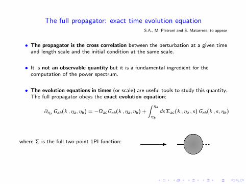
The full propagator: exact time evolution equationS.A., M. Pietroni and S. Matarrese, to appear

• The propagator is the cross correlation between the perturbation at a given timeand length scale and the initial condition at the same scale.

• It is not an observable quantity but it is a fundamental ingredient for thecomputation of the power spectrum.

• The evolution equations in times (or scale) are useful tools to study this quantity.The full propagator obeys the exact evolution equation:

∂ηa Gab(k , ηa, ηb) = −ΩacGcb(k , ηa, ηb) +

Z ηa

ηb

ds Σac (k , ηa , s) Gcb(k , s, ηb)

where Σ is the full two-point 1PI function:

Propagator in the large-k limit - linear PS (1)I We solve, in an approximate way, the propagator evolution equation.

I Take zin = 100: =⇒ consider only the leading time dependence (growing mode).

I In the large-k limit we resum all the infinite series of the dominant diagrams

I Each of the 2n vertixes contributes a factor: uc γacb(k,−q, q− k)large k−→ 1

2k·qq2 δab

⇒ Each loop integral decouples and the Diagrams ∼ k2n.

I In the large-k limit we compute the RHS of the exact evol. eq. at n-loop order

=⇒ we get the FACTORIZATION PROPERTY

n−1Xj=0

Z η

0dsΣ

(n−j)ac (k, η, s)G

(j)cb (k, s, 0)

large k−→ G(n−1)ab (k, η, 0)

Z η

0ds Σ

(1)ac (k, η, s)uc

Σ(1)ab ; (uc = 1, 1)

Propagator in the large-k limit - linear PS (2)

I Hence, summing over all the loop order, in the large-k limit we get

∂η Gab(k , η, 0) = −ΩacGcb(k , η, 0) + Gab(k , η, 0)

Z η

0ds Σ1−loop

ac (k , η , s)uc

whereR η

0 ds Σ(1)ac (k , η , s)uc

large k−→ −k2σ2v e2η and

σ2v ≡ 1

3

Rd3q P0(q)

q2 is the velocity dispersion.

I This result can be integrated to get

Gab(k, η, 0)large k−→ gab(η, 0)e

−k2σ2v e2η

2 .

I This matches with the diagrammatic results found by (Crocce & Scoccimarro,2006) obtained resumming the dominant diagrams about the propagator in thelarge-k limit

I With our approach, in a simple way, we can go beyond this diagrammaticresummation.

Propagator in the large-k limit - non linear PS

I In the previous computation we partially renormalized the vertex and thepropagator but we did not renomalize the PS.

=⇒ Now we take into account also the PS renormalization (in this way we avoidthe double counting problem).

=⇒ We consider the dominant diagrams with the non linear PS instead of thelinear one.

I Cause of this behavior: Ac γacb(k,−q, q− k)large k−→ A2

12

k·qq2 δab

⇒ Each loop integral decouples; the Diagrams ∼ k2n; only PNL22 is selected.

I We have shown that the FACTORIZATION PROPERTY STILL HOLDS

Propagator in the large-k limit - non linear PS

n−1Xj=0

Z η

0dsΣ

(n−j)ac (k, η, s)G

(j)cb (k, s, 0)

large k−→ G(n−1)ab (k, η, 0)

Z η

0ds Σ

(1)ac (k, η, s)uc

where now the up indexes count the number of the loops computed with the nonlinear PS (They don’t count the loops due to the renormalization of PSNL).

Σ(1)ab −→

I We get this new evolution equation

∂η Gab(k , η, 0) = −ΩacGcb(k , η, 0) + Gab(k , η, 0)

Z η

0ds Σ

(1)ac (k , η , s)uc

whereR η

0 ds Σ(1)ac (k , η , s)uc

large k−→ −k2σ2v (η)eη and

σ2v (η) ≡ 1

3

R η0 ds

Rd3q

PNL22 (q,η,s)

q2

Propagator in the small-k limit - linear PS

I In the small-k limit (large scale) high order contributions to the propagator aresuppressed, and linear perturbation theory is recovered.

⇒ We can compute the evolution equation at the 1-loop level.

I Modulo terms at least of two-loop order we get

∂η Gab(k , η, 0) = −ΩacGcb(k , η, 0) + Gab(k , η, 0)

Z η

0ds Σ

(1)ac (k , η , s)uc

=⇒ In the large and small k limit we get the same evolution equation

Propagator in the small-k limit - non linear PS (1)

I In general, with the non linear PS, the small-k limit of Σab is not zero.

=⇒ It doesn’t give the linear perturbation theory!!!

I FIRST EXAMPLE: If we consider PNL(k, η, s)=P1loop(k, η, s) we get

Σab

(1) + (2) + (3)small k−→ 0 but (4)

small k6= 0

If we take into account also this 2-loop diagram (easiest way)

Σ(V )ab

we get (1) + (2) + (3) + (4) + (V )small k−→ 0.

We have also the right limit for large k

ΣP1loop

ab = Σab + Σ(V )ab

where the Σ(V )ab contribution to ΣP1loop

ab is subdominant.

Propagator in the small-k limit - non linear PS (2)

I SECOND EXAMPLE

Resummed PS: PNL(k, η, s) = g(η, s)PTRG (k, s, s) (M. Pietroni, 2008).

Now we are resumming diagrams like these.

Σab

With this non linear PS we get automatically the right small-k limit.

Numerical Results: density propagator

To solve (numerically) the equations we take the PTRG non linear power spectrumcomputed in (M. Pietroni, 2008).

⇒ The density propagator slightly feel the effects of the non linear power spectrum.

Numerical Results: velocity propagator

I The effects of the non linear power spectrum are much important when wecompute the velocity propagator.

Short term goal: the power spectrum

The full power spectrum equation have this structure

Pab = P Iab + P II

ab

where

P Iab(k; ηa, ηb) = Gac (k; ηa, 0)Gbd (k; ηb, 0)P0

cd (k)

P IIab(k; ηa, ηb) =

Z ηa

0ds1

Z ηb

0ds2 Gac (k; ηa, s1)Gbd (k; ηb, s2)Φcd (k; s1, s2)

where Φ is the full two-point 1PI function:

I In the power spectrum computation the propagator is a fundamental keyingredient.

I The idea is to couple the time evolution equation of the power spectrum withthe time evolution equation of the propagator.

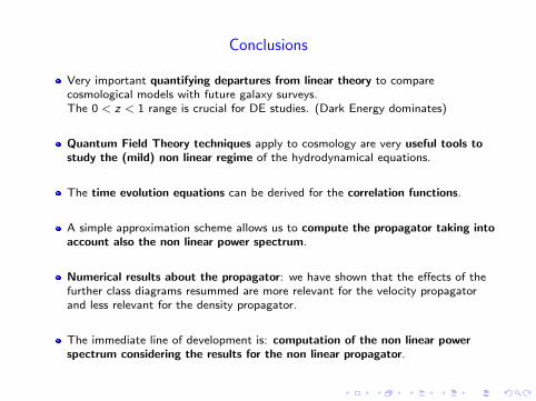
Conclusions

Very important quantifying departures from linear theory to comparecosmological models with future galaxy surveys.The 0 < z < 1 range is crucial for DE studies. (Dark Energy dominates)

Quantum Field Theory techniques apply to cosmology are very useful tools tostudy the (mild) non linear regime of the hydrodynamical equations.

The time evolution equations can be derived for the correlation functions.

A simple approximation scheme allows us to compute the propagator taking intoaccount also the non linear power spectrum.

Numerical results about the propagator: we have shown that the effects of thefurther class diagrams resummed are more relevant for the velocity propagatorand less relevant for the density propagator.

The immediate line of development is: computation of the non linear powerspectrum considering the results for the non linear propagator.