Convolutional LSTM Network: A Machine LearningApproach for Precipitation Nowcasting

Xingjian Shi Zhourong Chen Hao Wang Dit-Yan YeungDepartment of Computer Science and EngineeringHong Kong University of Science and Technology

{xshiab,zchenbb,hwangaz,dyyeung}@cse.ust.hk

Wai-kin Wong Wang-chun WooHong Kong Observatory

Hong Kong, China{wkwong,wcwoo}@hko.gov.hk

Abstract

The goal of precipitation nowcasting is to predict the future rainfall intensity in alocal region over a relatively short period of time. Very few previous studies haveexamined this crucial and challenging weather forecasting problem from the ma-chine learning perspective. In this paper, we formulate precipitation nowcastingas a spatiotemporal sequence forecasting problem in which both the input and theprediction target are spatiotemporal sequences. By extending the fully connectedLSTM (FC-LSTM) to have convolutional structures in both the input-to-state andstate-to-state transitions, we propose the convolutional LSTM (ConvLSTM) anduse it to build an end-to-end trainable model for the precipitation nowcasting prob-lem. Experiments show that our ConvLSTM network captures spatiotemporalcorrelations better and consistently outperforms FC-LSTM and the state-of-the-art operational ROVER algorithm for precipitation nowcasting.

1 Introduction

Nowcasting convective precipitation has long been an important problem in the field of weatherforecasting. The goal of this task is to give precise and timely prediction of rainfall intensity in alocal region over a relatively short period of time (e.g., 0-6 hours). It is essential for taking suchtimely actions as generating society-level emergency rainfall alerts, producing weather guidance forairports, and seamless integration with a longer-term numerical weather prediction (NWP) model.Since the forecasting resolution and time accuracy required are much higher than other traditionalforecasting tasks like weekly average temperature prediction, the precipitation nowcasting problemis quite challenging and has emerged as a hot research topic in the meteorology community [22].

Existing methods for precipitation nowcasting can roughly be categorized into two classes [22],namely, NWP based methods and radar echo1 extrapolation based methods. For the NWP approach,making predictions at the nowcasting timescale requires a complex and meticulous simulation ofthe physical equations in the atmosphere model. Thus the current state-of-the-art operational pre-cipitation nowcasting systems [19, 6] often adopt the faster and more accurate extrapolation basedmethods. Specifically, some computer vision techniques, especially optical flow based methods,have proven useful for making accurate extrapolation of radar maps [10, 6, 20]. One recent progressalong this path is the Real-time Optical flow by Variational methods for Echoes of Radar (ROVER)

1In real-life systems, radar echo maps are often constant altitude plan position indicator (CAPPI) images [9].

1

arX

iv:1

506.

0421

4v2

[cs

.CV

] 1

9 Se

p 20

15

algorithm [25] proposed by the Hong Kong Observatory (HKO) for its Short-range Warning ofIntense Rainstorms in Localized System (SWIRLS) [15]. ROVER calculates the optical flow ofconsecutive radar maps using the algorithm in [5] and performs semi-Lagrangian advection [4] onthe flow field, which is assumed to be still, to accomplish the prediction. However, the success ofthese optical flow based methods is limited because the flow estimation step and the radar echo ex-trapolation step are separated and it is challenging to determine the model parameters to give goodprediction performance.

These technical issues may be addressed by viewing the problem from the machine learning per-spective. In essence, precipitation nowcasting is a spatiotemporal sequence forecasting problemwith the sequence of past radar maps as input and the sequence of a fixed number (usually largerthan 1) of future radar maps as output.2 However, such learning problems, regardless of their exactapplications, are nontrivial in the first place due to the high dimensionality of the spatiotemporalsequences especially when multi-step predictions have to be made, unless the spatiotemporal struc-ture of the data is captured well by the prediction model. Moreover, building an effective predictionmodel for the radar echo data is even more challenging due to the chaotic nature of the atmosphere.

Recent advances in deep learning, especially recurrent neural network (RNN) and long short-termmemory (LSTM) models [12, 11, 7, 8, 23, 13, 18, 21, 26], provide some useful insights on howto tackle this problem. According to the philosophy underlying the deep learning approach, if wehave a reasonable end-to-end model and sufficient data for training it, we are close to solving theproblem. The precipitation nowcasting problem satisfies the data requirement because it is easyto collect a huge amount of radar echo data continuously. What is needed is a suitable model forend-to-end learning. The pioneering LSTM encoder-decoder framework proposed in [23] provides ageneral framework for sequence-to-sequence learning problems by training temporally concatenatedLSTMs, one for the input sequence and another for the output sequence. In [18], it is shown thatprediction of the next video frame and interpolation of intermediate frames can be done by buildingan RNN based language model on the visual words obtained by quantizing the image patches. Theypropose a recurrent convolutional neural network to model the spatial relationships but the modelonly predicts one frame ahead and the size of the convolutional kernel used for state-to-state tran-sition is restricted to 1. Their work is followed up later in [21] which points out the importanceof multi-step prediction in learning useful representations. They build an LSTM encoder-decoder-predictor model which reconstructs the input sequence and predicts the future sequence simultane-ously. Although their method can also be used to solve our spatiotemporal sequence forecastingproblem, the fully connected LSTM (FC-LSTM) layer adopted by their model does not take spatialcorrelation into consideration.

In this paper, we propose a novel convolutional LSTM (ConvLSTM) network for precipitation now-casting. We formulate precipitation nowcasting as a spatiotemporal sequence forecasting problemthat can be solved under the general sequence-to-sequence learning framework proposed in [23]. Inorder to model well the spatiotemporal relationships, we extend the idea of FC-LSTM to ConvLSTMwhich has convolutional structures in both the input-to-state and state-to-state transitions. By stack-ing multiple ConvLSTM layers and forming an encoding-forecasting structure, we can build anend-to-end trainable model for precipitation nowcasting. For evaluation, we have created a newreal-life radar echo dataset which can facilitate further research especially on devising machinelearning algorithms for the problem. When evaluated on a synthetic Moving-MNIST dataset [21]and the radar echo dataset, our ConvLSTM model consistently outperforms both the FC-LSTM andthe state-of-the-art operational ROVER algorithm.

2 Preliminaries

2.1 Formulation of Precipitation Nowcasting Problem

The goal of precipitation nowcasting is to use the previously observed radar echo sequence to fore-cast a fixed length of the future radar maps in a local region (e.g., Hong Kong, New York, or Tokyo).In real applications, the radar maps are usually taken from the weather radar every 6-10 minutes andnowcasting is done for the following 1-6 hours, i.e., to predict the 6-60 frames ahead. From the ma-

2It is worth noting that our precipitation nowcasting problem is different from the one studied in [14], whichaims at predicting only the central region of just the next frame.

2

chine learning perspective, this problem can be regarded as a spatiotemporal sequence forecastingproblem.

Suppose we observe a dynamical system over a spatial region represented by an M ×N grid whichconsists of M rows and N columns. Inside each cell in the grid, there are P measurements whichvary over time. Thus, the observation at any time can be represented by a tensor X ∈ RP×M×N ,where R denotes the domain of the observed features. If we record the observations periodically, wewill get a sequence of tensors X1, X2, . . . , Xt. The spatiotemporal sequence forecasting problem isto predict the most likely length-K sequence in the future given the previous J observations whichinclude the current one:

Xt+1, . . . , Xt+K = argmaxXt+1,...,Xt+K

p(Xt+1, . . . ,Xt+K | Xt−J+1, Xt−J+2, . . . , Xt) (1)

For precipitation nowcasting, the observation at every timestamp is a 2D radar echo map. If wedivide the map into tiled non-overlapping patches and view the pixels inside a patch as its measure-ments (see Fig. 1), the nowcasting problem naturally becomes a spatiotemporal sequence forecastingproblem.

We note that our spatiotemporal sequence forecasting problem is different from the one-step timeseries forecasting problem because the prediction target of our problem is a sequence which containsboth spatial and temporal structures. Although the number of free variables in a length-K sequencecan be up to O(MKNKPK), in practice we may exploit the structure of the space of possiblepredictions to reduce the dimensionality and hence make the problem tractable.

2.2 Long Short-Term Memory for Sequence Modeling

For general-purpose sequence modeling, LSTM as a special RNN structure has proven stable andpowerful for modeling long-range dependencies in various previous studies [12, 11, 17, 23]. Themajor innovation of LSTM is its memory cell ct which essentially acts as an accumulator of thestate information. The cell is accessed, written and cleared by several self-parameterized controllinggates. Every time a new input comes, its information will be accumulated to the cell if the input gateit is activated. Also, the past cell status ct−1 could be “forgotten” in this process if the forget gateft is on. Whether the latest cell output ct will be propagated to the final state ht is further controlledby the output gate ot. One advantage of using the memory cell and gates to control information flowis that the gradient will be trapped in the cell (also known as constant error carousels [12]) and beprevented from vanishing too quickly, which is a critical problem for the vanilla RNN model [12,17, 2]. FC-LSTM may be seen as a multivariate version of LSTM where the input, cell output andstates are all 1D vectors. In this paper, we follow the formulation of FC-LSTM as in [11]. The keyequations are shown in (2) below, where ‘◦’ denotes the Hadamard product:

it = σ(Wxixt +Whiht−1 +Wci ◦ ct−1 + bi)

ft = σ(Wxfxt +Whfht−1 +Wcf ◦ ct−1 + bf )

ct = ft ◦ ct−1 + it ◦ tanh(Wxcxt +Whcht−1 + bc)

ot = σ(Wxoxt +Whoht−1 +Wco ◦ ct + bo)

ht = ot ◦ tanh(ct)

(2)

Multiple LSTMs can be stacked and temporally concatenated to form more complex structures.Such models have been applied to solve many real-life sequence modeling problems [23, 26].

3 The Model

We now present our ConvLSTM network. Although the FC-LSTM layer has proven powerful forhandling temporal correlation, it contains too much redundancy for spatial data. To address thisproblem, we propose an extension of FC-LSTM which has convolutional structures in both theinput-to-state and state-to-state transitions. By stacking multiple ConvLSTM layers and forming anencoding-forecasting structure, we are able to build a network model not only for the precipitationnowcasting problem but also for more general spatiotemporal sequence forecasting problems.

3

2D Image 3D Tensor

P

P

Figure 1: Transforming 2D imageinto 3D tensor

Ht−1, Ct−1

Ht, Ct

Ht+1, Ct+1

Xt

Xt+1

Figure 2: Inner structure of ConvLSTM

3.1 Convolutional LSTM

The major drawback of FC-LSTM in handling spatiotemporal data is its usage of full connections ininput-to-state and state-to-state transitions in which no spatial information is encoded. To overcomethis problem, a distinguishing feature of our design is that all the inputs X1, . . . ,Xt, cell outputsC1, . . . , Ct, hidden states H1, . . . ,Ht, and gates it, ft, ot of the ConvLSTM are 3D tensors whoselast two dimensions are spatial dimensions (rows and columns). To get a better picture of the inputsand states, we may imagine them as vectors standing on a spatial grid. The ConvLSTM determinesthe future state of a certain cell in the grid by the inputs and past states of its local neighbors.This can easily be achieved by using a convolution operator in the state-to-state and input-to-statetransitions (see Fig. 2). The key equations of ConvLSTM are shown in (3) below, where ‘∗’ denotesthe convolution operator and ‘◦’, as before, denotes the Hadamard product:

it = σ(Wxi ∗ Xt +Whi ∗ Ht−1 +Wci ◦ Ct−1 + bi)

ft = σ(Wxf ∗ Xt +Whf ∗ Ht−1 +Wcf ◦ Ct−1 + bf )

Ct = ft ◦ Ct−1 + it ◦ tanh(Wxc ∗ Xt +Whc ∗ Ht−1 + bc)

ot = σ(Wxo ∗ Xt +Who ∗ Ht−1 +Wco ◦ Ct + bo)

Ht = ot ◦ tanh(Ct)

(3)

If we view the states as the hidden representations of moving objects, a ConvLSTM with a largertransitional kernel should be able to capture faster motions while one with a smaller kernel cancapture slower motions. Also, if we adopt a similar view as [16], the inputs, cell outputs and hiddenstates of the traditional FC-LSTM represented by (2) may also be seen as 3D tensors with the lasttwo dimensions being 1. In this sense, FC-LSTM is actually a special case of ConvLSTM with allfeatures standing on a single cell.

To ensure that the states have the same number of rows and same number of columns as the inputs,padding is needed before applying the convolution operation. Here, padding of the hidden states onthe boundary points can be viewed as using the state of the outside world for calculation. Usually,before the first input comes, we initialize all the states of the LSTM to zero which corresponds to“total ignorance” of the future. Similarly, if we perform zero-padding (which is used in this paper)on the hidden states, we are actually setting the state of the outside world to zero and assume no priorknowledge about the outside. By padding on the states, we can treat the boundary points differently,which is helpful in many cases. For example, imagine that the system we are observing is a movingball surrounded by walls. Although we cannot see these walls, we can infer their existence by findingthe ball bouncing over them again and again, which can hardly be done if the boundary points havethe same state transition dynamics as the inner points.

3.2 Encoding-Forecasting Structure

Like FC-LSTM, ConvLSTM can also be adopted as a building block for more complex structures.For our spatiotemporal sequence forecasting problem, we use the structure shown in Fig. 3 whichconsists of two networks, an encoding network and a forecasting network. Like in [21], the initialstates and cell outputs of the forecasting network are copied from the last state of the encodingnetwork. Both networks are formed by stacking several ConvLSTM layers. As our prediction targethas the same dimensionality as the input, we concatenate all the states in the forecasting networkand feed them into a 1× 1 convolutional layer to generate the final prediction.

We can interpret this structure using a similar viewpoint as [23]. The encoding LSTM compressesthe whole input sequence into a hidden state tensor and the forecasting LSTM unfolds this hidden

4

ConvLSTM2

Prediction

ConvLSTM1

Input

ConvLSTM4

ConvLSTM3

Encoding Network

Forecasting Network

Copy

Copy

Figure 3: Encoding-forecasting ConvLSTM network for precipitation nowcasting

state to give the final prediction:

Xt+1, . . . , Xt+K = argmaxXt+1,...,Xt+K

p(Xt+1, . . . ,Xt+K | Xt−J+1, Xt−J+2, . . . , Xt)

≈ argmaxXt+1,...,Xt+K

p(Xt+1, . . . ,Xt+K | fencoding(Xt−J+1, Xt−J+2, . . . , Xt))

≈ gforecasting(fencoding(Xt−J+1, Xt−J+2, . . . , Xt))

(4)

This structure is also similar to the LSTM future predictor model in [21] except that our input andoutput elements are all 3D tensors which preserve all the spatial information. Since the network hasmultiple stacked ConvLSTM layers, it has strong representational power which makes it suitablefor giving predictions in complex dynamical systems like the precipitation nowcasting problem westudy here.

4 Experiments

We first compare our ConvLSTM network with the FC-LSTM network on a synthetic Moving-MNIST dataset to gain some basic understanding of the behavior of our model. We run our modelwith different number of layers and kernel sizes and also study some “out-of-domain” cases asin [21]. To verify the effectiveness of our model on the more challenging precipitation nowcastingproblem, we build a new radar echo dataset and compare our model with the state-of-the-art ROVERalgorithm based on several commonly used precipitation nowcasting metrics. The results of theexperiments conducted on these two datasets lead to the following findings:

• ConvLSTM is better than FC-LSTM in handling spatiotemporal correlations.• Making the size of state-to-state convolutional kernel bigger than 1 is essential for capturing

the spatiotemporal motion patterns.• Deeper models can produce better results with fewer parameters.• ConvLSTM performs better than ROVER for precipitation nowcasting.

Our implementations of the models are in Python with the help of Theano [3, 1]. We run all theexperiments on a computer with a single NVIDIA K20 GPU. Also, more illustrative “gif” examplesare included in the appendix.

4.1 Moving-MNIST Dataset

For this synthetic dataset, we use a generation process similar to that described in [21]. All datainstances in the dataset are 20 frames long (10 frames for the input and 10 frames for the predic-tion) and contain two handwritten digits bouncing inside a 64 × 64 patch. The moving digits arechosen randomly from a subset of 500 digits in the MNIST dataset.3 The starting position and ve-locity direction are chosen uniformly at random and the velocity amplitude is chosen randomly in[3, 5). This generation process is repeated 15000 times, resulting in a dataset with 10000 trainingsequences, 2000 validation sequences, and 3000 testing sequences. We train all the LSTM mod-els by minimizing the cross-entropy loss4 using back-propagation through time (BPTT) [2] and

3MNIST dataset: http://yann.lecun.com/exdb/mnist/4The cross-entropy loss of the predicted frame P and the ground-truth frame T is defined as

−∑

i,j,k Ti,j,k logPi,j,k + (1− Ti,j,k) log(1− Pi,j,k).

5

Table 1: Comparison of ConvLSTM networks with FC-LSTM network on the Moving-MNISTdataset. ‘-5x5’ and ‘-1x1’ represent the corresponding state-to-state kernel size, which is either 5×5or 1×1. ‘256’, ‘128’, and ‘64’ refer to the number of hidden states in the ConvLSTM layers. ‘(5x5)’and ‘(9x9)’ represent the input-to-state kernel size.

Model Number of parameters Cross entropyFC-LSTM-2048-2048 142,667,776 4832.49ConvLSTM(5x5)-5x5-256 13,524,496 3887.94ConvLSTM(5x5)-5x5-128-5x5-128 10,042,896 3733.56ConvLSTM(5x5)-5x5-128-5x5-64-5x5-64 7,585,296 3670.85ConvLSTM(9x9)-1x1-128-1x1-128 11,550,224 4782.84ConvLSTM(9x9)-1x1-128-1x1-64-1x1-64 8,830,480 4231.50

Figure 4: An example showing an “out-of-domain” run. From left to right: input frames; groundtruth; prediction by the 3-layer network.

RMSProp [24] with a learning rate of 10−3 and a decay rate of 0.9. Also, we perform early-stoppingon the validation set.

Despite the simple generation process, there exist strong nonlinearities in the resulting dataset be-cause the moving digits can exhibit complicated appearance and will occlude and bounce duringtheir movement. It is hard for a model to give accurate predictions on the test set without learningthe inner dynamics of the system.

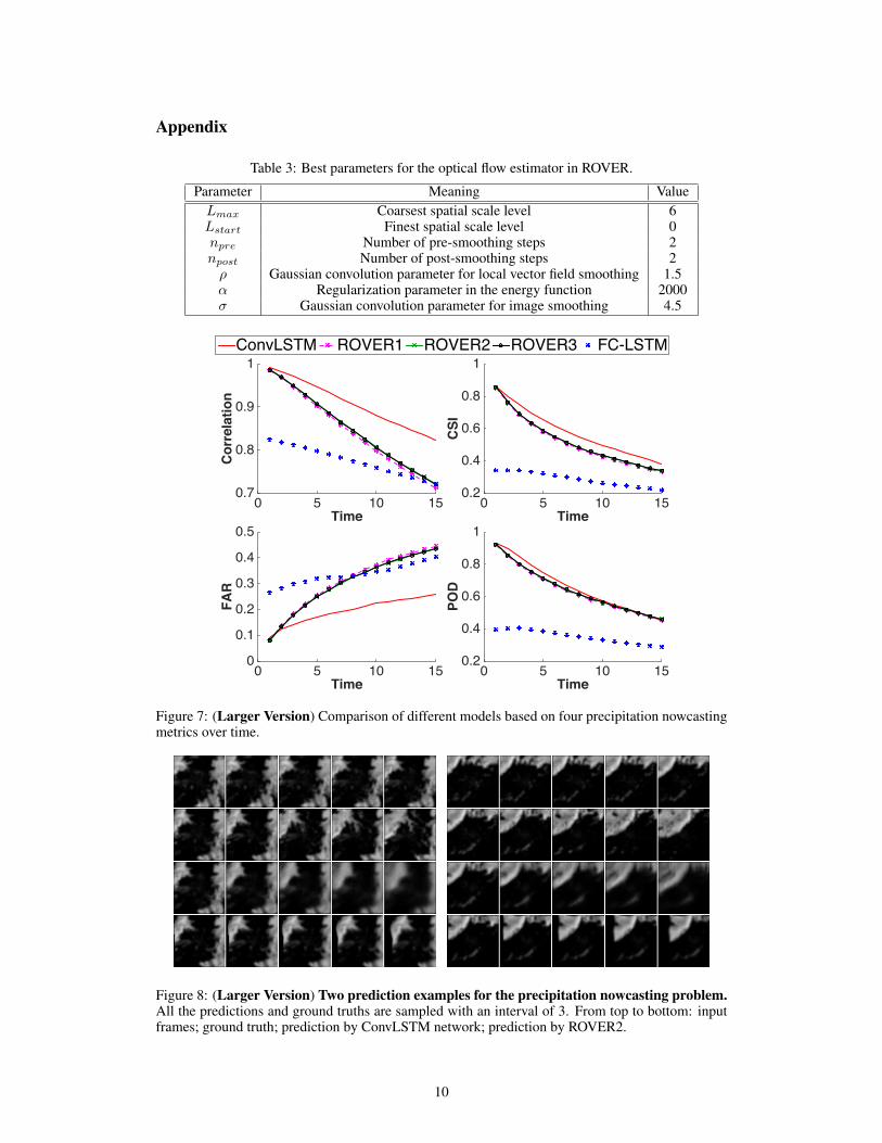
For the FC-LSTM network, we use the same structure as the unconditional future predictor modelin [21] with two 2048-node LSTM layers. For our ConvLSTM network, we set the patch size to4 × 4 so that each 64 × 64 frame is represented by a 16 × 16 × 16 tensor. We test three variantsof our model with different number of layers. The 1-layer network contains one ConvLSTM layerwith 256 hidden states, the 2-layer network has two ConvLSTM layers with 128 hidden states each,and the 3-layer network has 128, 64, and 64 hidden states respectively in the three ConvLSTMlayers. All the input-to-state and state-to-state kernels are of size 5 × 5. Our experiments showthat the ConvLSTM networks perform consistently better than the FC-LSTM network. Also, deepermodels can give better results although the improvement is not so significant between the 2-layerand 3-layer networks. Moreover, we also try other network configurations with the state-to-state andinput-to-state kernels of the 2-layer and 3-layer networks changed to 1 × 1 and 9 × 9, respectively.Although the number of parameters of the new 2-layer network is close to the original one, the resultbecomes much worse because it is hard to capture the spatiotemporal motion patterns with only 1×1state-to-state transition. Meanwhile, the new 3-layer network performs better than the new 2-layernetwork since the higher layer can see a wider scope of the input. Nevertheless, its performance isinferior to networks with larger state-to-state kernel size. This provides evidence that larger state-to-state kernels are more suitable for capturing spatiotemporal correlations. In fact, for 1× 1 kernel,the receptive field of states will not grow as time advances. But for larger kernels, later states havelarger receptive fields and are related to a wider range of the input. The average cross-entropy loss(cross-entropy loss per sequence) of each algorithm on the test set is shown in Table 1. We needto point out that our experiment setting is different from [21] where an infinite number of trainingdata is assumed to be available. The current offline setting is chosen in order to understand howdifferent models perform in occasions where not so much data is available. Comparison of the3-layer ConvLSTM and FC-LSTM in the online setting is included in the appendix.

6

Next, we test our model on some “out-of-domain” inputs. We generate another 3000 sequences ofthree moving digits, with the digits drawn randomly from a different subset of 500 MNIST digitsthat does not overlap with the training set. Since the model has never seen any system with threedigits, such an “out-of-domain” run is a good test of the generalization ability of the model [21].The average cross-entropy error of the 3-layer model on this dataset is 6379.42. By observing someof the prediction results, we find that the model can separate the overlapping digits successfullyand predict the overall motion although the predicted digits are quite blurred. One “out-of-domain”prediction example is shown in Fig. 10.

4.2 Radar Echo Dataset

The radar echo dataset used in this paper is a subset of the three-year weather radar intensitiescollected in Hong Kong from 2011 to 2013. Since not every day is rainy and our nowcasting targetis precipitation, we select the top 97 rainy days to form our dataset. For preprocessing, we firsttransform the intensity values Z to gray-level pixels P by setting P = Z−min{Z}

max{Z}−min{Z} and cropthe radar maps in the central 330 × 330 region. After that, we apply the disk filter5 with radius 10and resize the radar maps to 100 × 100. To reduce the noise caused by measuring instruments, wefurther remove the pixel values of some noisy regions which are determined by applying K-meansclustering to the monthly pixel average. The weather radar data is recorded every 6 minutes, so thereare 240 frames per day. To get disjoint subsets for training, testing and validation, we partition eachdaily sequence into 40 non-overlapping frame blocks and randomly assign 4 blocks for training, 1block for testing and 1 block for validation. The data instances are sliced from these blocks usinga 20-frame-wide sliding window. Thus our radar echo dataset contains 8148 training sequences,2037 testing sequences and 2037 validation sequences and all the sequences are 20 frames long (5for the input and 15 for the prediction). Although the training and testing instances sliced from thesame day may have some dependencies, this splitting strategy is still reasonable because in real-lifenowcasting, we do have access to all previous data, including data from the same day, which allowsus to apply online fine-tuning of the model. Such data splitting may be viewed as an approximationof the real-life “fine-tuning-enabled” setting for this application.

We set the patch size to 2 and train a 2-layer ConvLSTM network with each layer containing 64hidden states and 3 × 3 kernels. For the ROVER algorithm, we tune the parameters of the opticalflow estimator6 on the validation set and use the best parameters (shown in the appendix) to report thetest results. Also, we try three different initialization schemes for ROVER: ROVER1 computes theoptical flow of the last two observed frames and performs semi-Lagrangian advection afterwards;ROVER2 initializes the velocity by the mean of the last two flow fields; and ROVER3 gives theinitialization by a weighted average (with weights 0.7, 0.2 and 0.1) of the last three flow fields. Inaddition, we train an FC-LSTM network with two 2000-node LSTM layers. Both the ConvLSTMnetwork and the FC-LSTM network optimize the cross-entropy error of 15 predictions.

We evaluate these methods using several commonly used precipitation nowcasting metrics, namely,rainfall mean squared error (Rainfall-MSE), critical success index (CSI), false alarm rate (FAR),probability of detection (POD), and correlation. The Rainfall-MSE metric is defined as the averagesquared error between the predicted rainfall and the ground truth. Since our predictions are done atthe pixel level, we project them back to radar echo intensities and calculate the rainfall at every cell ofthe grid using the Z-R relationship [15]: Z = 10 log a+10b logR, where Z is the radar echo inten-sity in dB, R is the rainfall rate in mm/h, and a, b are two constants with a = 118.239, b = 1.5241.The CSI, FAR and POD are skill scores similar to precision and recall commonly used by machinelearning researchers. We convert the prediction and ground truth to a 0/1 matrix using a thresholdof 0.5mm/h rainfall rate (indicating raining or not) and calculate the hits (prediction = 1, truth = 1),misses (prediction = 0, truth = 1) and false alarms (prediction = 1, truth = 0). The three skill scoresare defined as CSI = hits

hits+misses+falsealarms , FAR = falsealarmshits+falsealarms , POD = hits

hits+misses . The cor-

relation of a predicted frame P and a ground-truth frame T is defined as∑

i,j Pi,jTi,j√(∑

i,j P 2i,j)(

∑i,j T 2

i,j)+ε

where ε = 10−9.

5The disk filter is applied using the MATLAB function fspecial(’disk’, 10).6We use an open-source project to calculate the optical flow: http://sourceforge.net/

projects/varflow/

7

Table 2: Comparison of the average scores of different models over 15 prediction steps.Model Rainfall-MSE CSI FAR POD CorrelationConvLSTM(3x3)-3x3-64-3x3-64 1.420 0.577 0.195 0.660 0.908Rover1 1.712 0.516 0.308 0.636 0.843Rover2 1.684 0.522 0.301 0.642 0.850Rover3 1.685 0.522 0.301 0.642 0.849FC-LSTM-2000-2000 1.865 0.286 0.335 0.351 0.774

Time0 5 10 15

FAR

0

0.1

0.2

0.3

0.4

0.5

Time0 5 10 15

POD

0.2

0.4

0.6

0.8

1

ConvLSTM ROVER1 ROVER2 ROVER3 FC-LSTM

Time0 5 10 15

Correlation

0.7

0.8

0.9

1

Time0 5 10 15

CSI

0.2

0.4

0.6

0.8

1

Figure 5: Comparison of different modelsbased on four precipitation nowcasting met-rics over time.

Figure 6: Two predicion examples for the pre-cipitation nowcasting problem. All the pre-dictions and ground truths are sampled with aninterval of 3. From top to bottom: input frames;ground truth frames; prediction by ConvLSTMnetwork; prediction by ROVER2.

All results are shown in Table 2 and Fig. 5. We can find that the performance of the FC-LSTMnetwork is not so good for this task, which is mainly caused by the strong spatial correlation in theradar maps, i.e., the motion of clouds is highly consistent in a local region. The fully-connectedstructure has too many redundant connections and makes the optimization very unlikely to capturethese local consistencies. Also, it can be seen that ConvLSTM outperforms the optical flow basedROVER algorithm, which is mainly due to two reasons. First, ConvLSTM is able to handle theboundary conditions well. In real-life nowcasting, there are many cases when a sudden agglom-eration of clouds appears at the boundary, which indicates that some clouds are coming from theoutside. If the ConvLSTM network has seen similar patterns during training, it can discover thistype of sudden changes in the encoding network and give reasonable predictions in the forecastingnetwork. This, however, can hardly be achieved by optical flow and semi-Lagrangian advectionbased methods. Another reason is that, ConvLSTM is trained end-to-end for this task and somecomplex spatiotemporal patterns in the dataset can be learned by the nonlinear and convolutionalstructure of the network. For the optical flow based approach, it is hard to find a reasonable way toupdate the future flow fields and train everything end-to-end. Some prediction results of ROVER2and ConvLSTM are shown in Fig. 6. We can find that ConvLSTM can predict the future rainfallcontour more accurately especially in the boundary. Although ROVER2 can give sharper predic-tions than ConvLSTM, it triggers more false alarms and is less precise than ConvLSTM in general.Also, the blurring effect of ConvLSTM may be caused by the inherent uncertainties of the task, i.e,it is almost impossible to give sharp and accurate predictions of the whole radar maps in longer-termpredictions. We can only blur the predictions to alleviate the error caused by this type of uncertainty.

5 Conclusion and Future Work

In this paper, we have successfully applied the machine learning approach, especially deep learning,to the challenging precipitation nowcasting problem which so far has not benefited from sophisti-cated machine learning techniques. We formulate precipitation nowcasting as a spatiotemporal se-quence forecasting problem and propose a new extension of LSTM called ConvLSTM to tackle theproblem. The ConvLSTM layer not only preserves the advantages of FC-LSTM but is also suitablefor spatiotemporal data due to its inherent convolutional structure. By incorporating ConvLSTMinto the encoding-forecasting structure, we build an end-to-end trainable model for precipitationnowcasting. For future work, we will investigate how to apply ConvLSTM to video-based actionrecognition. One idea is to add ConvLSTM on top of the spatial feature maps generated by a con-volutional neural network and use the hidden states of ConvLSTM for the final classification.

8

References[1] F. Bastien, P. Lamblin, R. Pascanu, J. Bergstra, I. Goodfellow, A. Bergeron, N. Bouchard, D. Warde-

Farley, and Y. Bengio. Theano: New features and speed improvements. Deep Learning and UnsupervisedFeature Learning NIPS 2012 Workshop, 2012.

[2] Y. Bengio, I. Goodfellow, and A. Courville. Deep Learning. Book in preparation for MIT Press, 2015.

[3] J. Bergstra, O. Breuleux, F. Bastien, P. Lamblin, R. Pascanu, G. Desjardins, J. Turian, D. Warde-Farley,and Y. Bengio. Theano: a CPU and GPU math expression compiler. In Scipy, volume 4, page 3. Austin,TX, 2010.

[4] R. Bridson. Fluid Simulation for Computer Graphics. Ak Peters Series. Taylor & Francis, 2008.

[5] T. Brox, A. Bruhn, N. Papenberg, and J. Weickert. High accuracy optical flow estimation based on atheory for warping. In ECCV, pages 25–36. 2004.

[6] P. Cheung and H.Y. Yeung. Application of optical-flow technique to significant convection nowcast forterminal areas in Hong Kong. In the 3rd WMO International Symposium on Nowcasting and Very Short-Range Forecasting (WSN12), pages 6–10, 2012.

[7] K. Cho, B. van Merrienboer, C. Gulcehre, F. Bougares, H. Schwenk, and Y. Bengio. Learning phraserepresentations using RNN encoder-decoder for statistical machine translation. In EMNLP, pages 1724–1734, 2014.

[8] J. Donahue, L. A. Hendricks, S. Guadarrama, M. Rohrbach, S. Venugopalan, K. Saenko, and T. Darrell.Long-term recurrent convolutional networks for visual recognition and description. In CVPR, 2015.

[9] R. H. Douglas. The stormy weather group (Canada). In Radar in Meteorology, pages 61–68. 1990.

[10] Urs Germann and Isztar Zawadzki. Scale-dependence of the predictability of precipitation from continen-tal radar images. Part I: Description of the methodology. Monthly Weather Review, 130(12):2859–2873,2002.

[11] A. Graves. Generating sequences with recurrent neural networks. arXiv preprint arXiv:1308.0850, 2013.

[12] S. Hochreiter and J. Schmidhuber. Long short-term memory. Neural Computation, 9(8):1735–1780,1997.

[13] A. Karpathy and L. Fei-Fei. Deep visual-semantic alignments for generating image descriptions. InCVPR, 2015.

[14] B. Klein, L. Wolf, and Y. Afek. A dynamic convolutional layer for short range weather prediction. InCVPR, 2015.

[15] P.W. Li, W.K. Wong, K.Y. Chan, and E. S.T. Lai. SWIRLS-An Evolving Nowcasting System. Hong KongSpecial Administrative Region Government, 2000.

[16] J. Long, E. Shelhamer, and T. Darrell. Fully convolutional networks for semantic segmentation. In CVPR,2015.

[17] R. Pascanu, T. Mikolov, and Y. Bengio. On the difficulty of training recurrent neural networks. In ICML,pages 1310–1318, 2013.

[18] M. Ranzato, A. Szlam, J. Bruna, M. Mathieu, R. Collobert, and S. Chopra. Video (language) modeling: abaseline for generative models of natural videos. arXiv preprint arXiv:1412.6604, 2014.

[19] M. Reyniers. Quantitative Precipitation Forecasts Based on Radar Observations: Principles, Algorithmsand Operational Systems. Institut Royal Meteorologique de Belgique, 2008.

[20] H. Sakaino. Spatio-temporal image pattern prediction method based on a physical model with time-varying optical flow. IEEE Transactions on Geoscience and Remote Sensing, 51(5-2):3023–3036, 2013.

[21] N. Srivastava, E. Mansimov, and R. Salakhutdinov. Unsupervised learning of video representations usinglstms. In ICML, 2015.

[22] J. Sun, M. Xue, J. W. Wilson, I. Zawadzki, S. P. Ballard, J. Onvlee-Hooimeyer, P. Joe, D. M. Barker,P. W. Li, B. Golding, M. Xu, and J. Pinto. Use of NWP for nowcasting convective precipitation: Recentprogress and challenges. Bulletin of the American Meteorological Society, 95(3):409–426, 2014.

[23] I. Sutskever, O. Vinyals, and Q. V. Le. Sequence to sequence learning with neural networks. In NIPS,pages 3104–3112, 2014.

[24] T. Tieleman and G. Hinton. Lecture 6.5 - RMSProp: Divide the gradient by a running average of its recentmagnitude. Coursera Course: Neural Networks for Machine Learning, 4, 2012.

[25] W.C. Woo and W.K. Wong. Application of optical flow techniques to rainfall nowcasting. In the 27thConference on Severe Local Storms, 2014.

[26] K. Xu, J. Ba, R. Kiros, A. Courville, R. Salakhutdinov, R. Zemel, and Y. Bengio. Show, attend and tell:Neural image caption generation with visual attention. In ICML, 2015.

9

Appendix

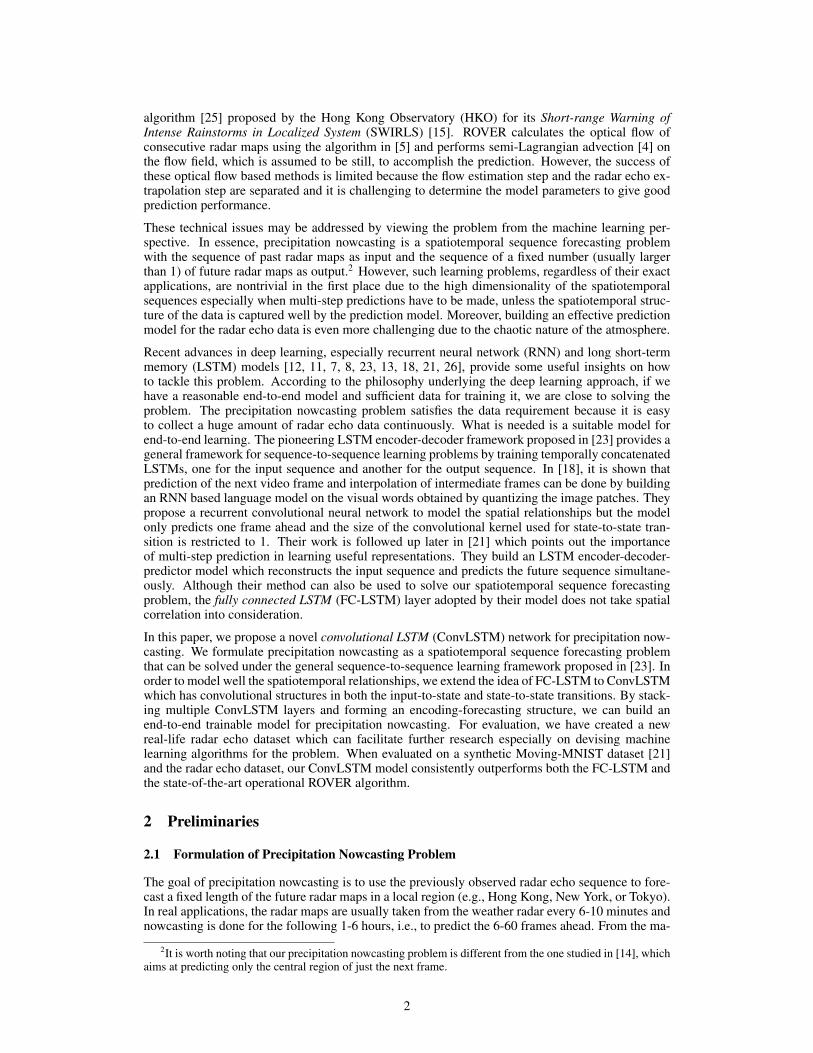
Table 3: Best parameters for the optical flow estimator in ROVER.

Parameter Meaning ValueLmax Coarsest spatial scale level 6Lstart Finest spatial scale level 0npre Number of pre-smoothing steps 2npost Number of post-smoothing steps 2ρ Gaussian convolution parameter for local vector field smoothing 1.5α Regularization parameter in the energy function 2000σ Gaussian convolution parameter for image smoothing 4.5

Time0 5 10 15

FAR

0

0.1

0.2

0.3

0.4

0.5

Time0 5 10 15

POD

0.2

0.4

0.6

0.8

1

ConvLSTM ROVER1 ROVER2 ROVER3 FC-LSTM

Time0 5 10 15

Correlation

0.7

0.8

0.9

1

Time0 5 10 15

CSI

0.2

0.4

0.6

0.8

1

Figure 7: (Larger Version) Comparison of different models based on four precipitation nowcastingmetrics over time.

Figure 8: (Larger Version) Two prediction examples for the precipitation nowcasting problem.All the predictions and ground truths are sampled with an interval of 3. From top to bottom: inputframes; ground truth; prediction by ConvLSTM network; prediction by ROVER2.

10

Figure 9: An illustrative example showing the in-domain prediction results of differentmodels. From top to bottom: input frames; ground truth; FC-LSTM; ConvLSTM-5X5-5X5-1-layer; ConvLSTM-5X5-5X5-2-layer; ConvLSTM-5X5-5X5-3-layer; ConvLSTM-9X9-1X1-2-layer; ConvLSTM-9X9-1X1-3-layer.

Figure 10: (Larger Version) An illustrative example showing an out-domain run. From top tobottom: input frames; ground truth; predictions of the 3-layer network.

11

Data Cases ×1051 2 3 4 5 6 7

Ave

rage

Cro

ss E

ntro

py

2000

3000

4000

5000

6000

7000

ConvLSTM

FC-LSTM

Figure 11: Comparison of the 3-layer ConvLSTM and FC-LSTM in the online setting. In eachiteration, we generate a new set of training samples and record the average cross entropy of thatmini-batch. The x-axis is the number of data cases (starting from 25600) and the y-axis is theaverage cross entropy of the mini-batches. We can find that the loss of ConvLSTM decreases fasterthan FC-LSTM.

12