Abreu Matsushima Mechanisms: Experimental Evidenceecon.ucsd.edu/~jandreon/Econ264/papers/Sefton...

GAMES AND ECONOMIC BEHAVIOR16,280–302 (1996)ARTICLE NO. 0087

Abreu–Matsushima Mechanisms: Experimental Evidence∗

Martin Sefton

School of Economic Studies, University of Manchester, Manchester, M13 9PL, United Kingdom

and

Abdullah Yavas

Smeal College of Business, Pennsylvania State University, University Park, Pennsylvania16802

Received April 12, 1995

Abreu–Matsushima mechanisms can be applied to a broad class of games to induce anydesired outcome as the unique rationalizable outcome. We conduct experiments investigat-ing the performance of such mechanisms in two simple coordination games. In these gamesone pure-strategy equilibrium is “focal”; we assess the efficacy of Abreu–Matsushima mech-anisms for implementing the other pure-strategy equilibrium outcome. Abreu–Matsushimamechanisms induce some choices consistent with the desired outcome, but more choicesreflect the focal outcome. Moreover, “strengthening” the mechanism has a perverse effectwhen the desired outcome is a Pareto-dominated risk-dominated equilibrium.Journal ofEconomic LiteratureClassification Number: C7. © 1996 Academic Press, Inc.

1. INTRODUCTION

It is well known that a group of individuals independently pursuing their owninterests may fail to attain an outcome that promotes the group’s interests. Insuch situations it is natural to seek mechanisms that change individual incentives,thereby leading to a better outcome for the group. Consequently a large theoreti-cal literature has emerged devoted to designing and evaluating such mechanisms.

∗ Financial support from the Institute for Real Estate Studies at the Pennsylvania State University isgratefully acknowledged. Donna Chaklos, Tom Geurts, Brian Moran, Mary Ann Morris, and ShiaweeYang provided valuable research assistance. The authors thank Gary Bolton, Robert Forsythe, AnnGillette, Robert Rosethal, two anonymous referees, and seminar participants at Penn State University,University of Manchester, University of Windsor, 1994 European Econometric Society Meetings, andthe Seventh World Congress of the Econometric Society for their comments. E-mail address for firstauthor: [email protected].

2800899-8256/96 $18.00Copyright © 1996 by Academic Press, Inc.All rights of reproduction in any form reserved.

ABREU–MATSUSHIMA MECHANISMS: EXPERIMENTAL EVIDENCE 281

In this paper we present an experimental investigation of the mechanism in-troduced by Abreu and Matsushima (1992a). This mechanism can be used toimplement any outcome of a broad class of games as a unique rationalizableoutcome. The mechanism uses two elements to implement the desired outcomeof a game. First, it forces the players to play the game in very small pieces;second, it levies fines on the first player(s) whose behavior leads to divergencefrom the desired outcome. As we shall explain in the next section, this impliesthat even a very small fine can be effective if the game is broken into sufficientlymany pieces. In fact, such a fine achieves its goal through iterative eliminationof strictly dominated strategies.

The applicability of the mechanism has, however, been criticized. Glazer andRosenthal (1992); hereafter, GR) argue that the mechanism will not performas predicted because it may involve many rounds of iterated dominance. Theyillustrate their argument by considering whether the mechanism could be usedto implement the Pareto-dominated and risk-dominated equilibrium of a coordi-nation game. They suspect that the players “would abandon the logic of iterateddominance in favor of the focal point in this game.” In a response to GR, Abreuand Matsushima (1992b; hereafter, AM) disagree. However, this dispute aboutthe performance of the mechanism is entirely speculative: the disagreement con-cerns how subjectswoudbehave in a carefully controlled experiment.

In order to lend empirical substance to this dispute, we conducted an exper-iment in which a mechanism was incorporated into the game they discuss: wetested the ability of the mechanism to implement the Pareto-dominated and risk-dominated equilibrium of a coordination game. We also investigated the impactof varying the number of pieces into which the game is broken. The logic ofAM suggests that dividing the game into a greater number of pieces amplifiesthe effect of a given fine, thus enhancing the performance of the mechanism.However, as the number of pieces increases, the number of rounds of iterateddominance required to implement the desired outcome also increases, and thisis the basis of the GR critique.

We find significant differences between actual behavior and predicted behav-ior. A negligible portion of the decisions correspond to the theoretical prediction.Moreover, the effect of varying the number of pieces is interesting. As we in-crease the number of pieces, the degree of success of the mechanism did notimprove, contrary to what one would expect on theoretical grounds. Instead,our results are consistent with the notion that people only carry out iterateddominance arguments for a limited number of iterations.

This experiment represents an extremely special implementation problem: theplanner’s objective is to implement aPareto-inferioroutcome. A more naturalimplementation problem is suggested by the experimental results of coordinationgames in which the Pareto-dominant equilibrium is risk-dominated (see Cooperet al., 1992; Straub, 1995; and Sefton and Yava¸s, 1995). In these experimentscoordination failuresare prevalent—subjects tend to play the Pareto-dominated

282 SEFTON AND YAVAS

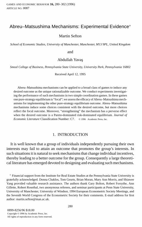
FIG. 1. Payoff Matrix for Game I.

equilibrium. A natural question to ask is whether an Abreu-Matsushima mech-anism can resolve such coordination failures. We investigated this question ina second experiment where we attempted to implement the Pareto-dominant,but risk-dominated, equilibrium of a coordination game. Neither AM nor GRdisputes the ability of the mechanism to implement such an outcome. Neverthe-less, given our results from the first experiment, we were uncertain about theeffectiveness of the mechanism in such a setting.

Our results for this game are less clear. Although the mechanism was moresuccessful in implementing the desired outcome than that in our first experiment,the theoretical prediction is still a poor predictor of behavior. On the other hand,unlike in our first experiment and consistent with the logic of AM, dividing thegame into a larger number of pieces resulted in a higher success rate for themechanism.

The remainder of the paper is organized as follows. The Abreu–Matsushimamechanism is presented in Section 2. We describe the experimental design inSection 3 and the experimental procedures in Section 4. The experimental resultsare reported in Section 5, and in Section 6 we provide some concluding remarks.

2. THE ABREU–MATSUSHIMA MECHANISM

Abreu and Matsushima (1992a) introduce a mechanism that implements anydesired outcome of a broad class of games as a unique Nash equilibrium. Infact, implementation is achieved via the iterative deletion of strictly dominatedstrategies so that the desired outcome is also the unique rationalizable outcome.However, a unique Nash equilibrium, and even a unique rationalizable outcome,can be an implausible predictor of actual behavior. This is particularly truewhen predictions are based on many rounds of iterated dominance (see Kreps,1990, pp. 393–399; or Basu, 1994). The GR paper argues that when the Abreu–Matsushima mechanism implements an outcome, it does so in a way which issusceptible to this criticism. They illuminate their argument using the two-playercoordination game with payoff matrix given in Fig. 1. We will refer to this gameas Game I.


Game I has multiple Nash equilibria which cannot be narrowed down usingstability and coarser refinement criteria. However, most observers expect playersto choose red in this game. The concepts of risk dominance and Pareto dominance(see Harsanyi and Selten, 1988) can be used to support such expectations, andso we identify (red,red) as the focal equilibrium of Game I.1

Now, suppose a planner’s objective is to implement the (blue, blue) equilib-rium. An Abreu–Matsushima mechanism would accomplish this objective bydividing the game into many pieces and introducing a small fine. Specifically,each player submits a sequence ofT choices, instead of a single choice, of redor blue. The sequences are then matched, first choice of the row player with firstchoice of the column player, second choice with second choice, and so on. Foreach (red,red) combination the players receive a payoff of 480/T each, for each(blue, blue) combination the players receive 240/T each, and for other combi-nations the players receive nothing. In addition, a player pays a fine ofF if theearliest choice of red in his or her sequence occurs before that of his or her oppo-nent. Both players pay the fine if their earliest choices of red occur at the sametime. If F > 480/T the unique rationalizable outcome, determined by iterativeelimination of strictly dominated strategies, consists of both players choosing asequence ofT blues. In this sense, even an arbitrarily small fine can implement(blue, blue) as the unique rationalizable outcome, as long asT is large enough.Note that the fine is never actually used in equilibrium.

Whether subjects in a carefully controlled experiment will play the assignedequilibrium is an empirical question upon which GR and AM disagree. WhileGR “would hesitate to give long odds” on successful implementation, AM’s “gutinstinct is that our mechanism will not fare poorly in terms of the essential featureof their construction.” The effect of varyingF , givenT , is not controversial—itseems reasonable to suppose that increasing the penalty on the earliest choice ofred will reduce its incidence. Rather, it is the effect of varyingT , givenF , that iscontroversial. According to the logic of AM, increasingT multiplies the effectof a given fine.2 Thus, a given fine may implement (blue,blue) whenT is largebut not whenT is small. On the other hand, whenT increases, the number ofrounds of iterated dominance required to implement (blue, blue) increases. Thusthe rationality assumption required to implement (blue,blue) becomes stronger.3

This controversy seems a prime candidate for an experimental test.While the example nicely illustrates the dispute, it involves an unusual plan-

1 In fact, in a preliminary experiment in which 12 pairs of subjects played Game I once, Red waschosen 22 of 24 times. We interpret this as supporting our interpretation of (red,red) as the focalequilibrium, although the two rogue decisions should be noted.

2 For a givenF , asT increases, 480/T becomes smaller relative toF . This is expected to increasethe incentive for each player to play his or her earliest choice of red after that of the other player.

3 The rationality requirement is that “each player knows the other player knows. . . knows the otherplayer is rational”, the length of the sentence growing with the number of iterations of dominance.


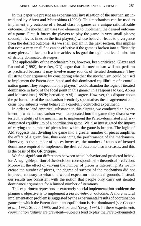
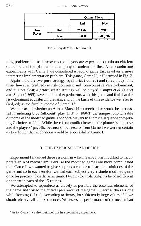
FIG. 2. Payoff Matrix for Game II.

ning problem: left to themselves the players are expected to attain an efficientoutcome, and the planner is attempting to undermine this. After conductingexperiments with Game I we considered a second game that involves a moreinteresting implementation problem. This game, Game II, is illustrated in Fig. 2.

Again there are two pure-strategy equilibria, (red,red) and (blue,blue). Thistime, however, (red,red) is risk-dominant and (blue,blue) is Pareto-dominant,and it is not clear,a priori, which strategy will be played. Cooperet al. (1992)and Straub (1995) have conducted experiments with this game and find that therisk-dominant equilibrium prevails, and on the basis of this evidence we refer to(red,red) as the focal outcome of Game II.4

We then asked whether an Abreu–Matsushima mechanism would be success-ful in inducing blue (efficient) play. IfF > 960/T the unique rationalizableoutcome of the modified game is for both players to submit a sequence compris-ing T choices of blue. While there is no conflict between the planner’s objectiveand the players’ payoffs, because of our results from Game I we were uncertainas to whether the mechanism would be successful in Game II.

3. THE EXPERIMENTAL DESIGN

Experiment I involved three sessions in which Game I was modified to incor-porate an AM mechanism. Because the modified games are more complicatedthan Game I, we wanted to give subjects a chance to learn the subtleties of thegame and so in each session we had each subject play a single modified gameonce for practice, then the same game 14 times for cash. Subjects faced a differentopponent in each of the 15 rounds.

We attempted to reproduce as closely as possible the essential elements ofthe game and varied the critical parameter of the game,T , across the sessionswhile keepingF fixed. According to theory, for sufficiently large values ofT weshould observe all-blue sequences. We assess the performance of the mechanism

4 As for Game I, we also confirmed this in a preliminary experiment.


by testing whether the prevalence of blue play increases withT , in line with thiscomparative static prediction.

Both GR and AM discussed a mechanism withT = 100, but given the diffi-culties associated with making, communicating, and computing the payoffs froma game with such a large number of choices, we considered this infeasible forexperimental purposes. Instead, we conducted sessions of games withT = 4,8, and 12 (we denote these sessions by 4T, 8T, and 12T); we see no reasonwhy using shorter sequences should prejudice the experiment against successfulimplementation.

Using shorter sequences means that larger fines are required to implement(blue,blue). We were concerned that with large fines (relative to the equilibriumpayoffs) blue play may be induced for reasons unrelated to the essential “piecedplay” feature of the mechanism. For this reason we setF = 90 so that (red,red)remains risk-dominant in theT = 1 game with a fine. (Straub, 1995, presentscompelling evidence that a payoff-dominant outcome will be observed in ex-periments with this type of game if it is also risk-dominant.) With this fine, theall-blue outcome is uniquely rationalizable forT ≥ 6.

With these parameters, we can observe whether blue play is more likely whenthe mechanism implements (blue, blue) than when it does not. Further, we caninvestigate whether strengthening the mechanism, by increasingT , improvesits performance.5 We do this by comparing the prevalence of blue play acrosssessions.

For Experiment II we again conducted three sessions, withT = 4, 8, 12. Theprocedures were identical to those used for Experiment I, except for the payoffsand fine. The payoffs were derived from Game II, and the fine was set atF = 160,so that, as in Experiment I, the all-blue outcome is uniquely rationalizable forT ≥ 6. Again, we are able to assess whether there is more blue play when themechanism implements (blue,blue) than when it does not, as well as assessingwhether blue play increases when the mechanism is strengthened.

In summary, Experiment I consists of three sessions of Game I, spread over 4,8, and 12 pieces, respectively, with a 90 point fine. With this fine the 8T and 12Tgames implement (blue,blue), but the 4T game does not.6 Experiment II consistsof three sessions of Game II, spread over 4, 8, and 12 pieces respectively, with a160 point fine. Again, this fine implements (blue,blue) in the 8T and 12T games,but not in the 4T game.

5 Another possibility for strengthening the mechanism is to increase the fine, as discussed by AM.We expect that, givenT , there is a level of fine sufficiently large to induce all-blue play. However, thequestion of more interest is whether, givenF , there is a level ofT sufficiently large to induce all-blueplay. Thus, we preferred to manipulate the incentive to delay red choices by varyingT .

6 In the 4T games the best response of a player is to produce a sequence identical to that of his/heropponent. Thus, (blue,blue) is only one of many equilibria in this game.


4. EXPERIMENTAL PROCEDURES7

Experiment I was conducted in September 1993 and Experiment II in March1994 at Pennsylvania State University. Each experiment used 90 subjects, 30 ineach of three sessions, who had signed up in response to fliers posted aroundcampus. Each subject participated in one session only. In each session 30 subjectswere seated in a large room, read a set of instructions, and given an opportunityto ask questions. We then conducted a practice round in which earnings werehypothetical, and at the end of this practice round we gave subjects anotheropportunity to ask questions. A partition was then drawn to divide the room intotwo halves, and this completed the instructional part of the session.

Each session consisted of 15 rounds (including the practice round), with sub-jects rematched with a new, anonymous opponent after each round. The pairingswere also designed to prohibit indirect repeated interactions through commonopponents of opponents. Thus, at the beginning of any round, a subject couldnot have been affected in any way by the previous play of their new opponent.In this sense, we refer to the 15 games played by a subject as a sequence ofone-shot games.8 Throughout each session the only permitted communicationbetween subjects was via their formal decisions.

In each round of a session each subject made a decision consisting ofT choicesof red and/or blue and recorded it. When all subjects had done this, monitorsdelivered the decision forms to the appropriate subjects. Subjects then computedtheir earnings, and monitors checked their calculations. The next round did notbegin until the monitors had verified that all subjects had calculated their earningscorrectly.

Subjects started the session with an initial balance of 1600 points in Experi-ment I (2000 points in Experiment II) and accumulated additional points throughthe outcome of the games they played. At the end of the session they were paid$0.25 per 100 points in Experiment I ($0.25 per 250 points in Experiment II).The sessions averaged 85 min, and earnings averaged $12.60 in Experiment I($13.80 in Experiment II).

5. EXPERIMENTAL RESULTS9

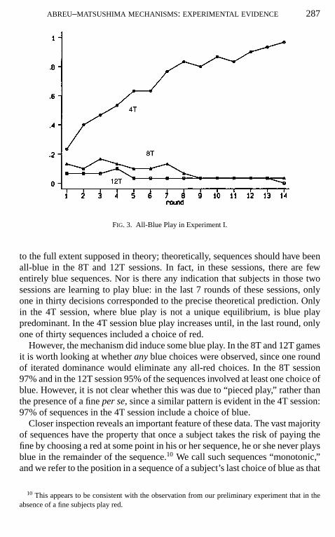
Figure 3 displays the proportion of entirely blue sequences in Experiment Iacross rounds. It is clear that the process of iterated dominance does not work

7 A full set of experimental materials is included in Appendices 1 and 2.8 Of course, subjects may havethoughttheir current decision could influence future opponents’ play.

We are skeptical that subjects would modify their play on the basis of such (incorrect) beliefs).9 We exclude the data from the practice round from all calculations in this section. A complete set

of the data is available from either author upon request.


FIG. 3. All-Blue Play in Experiment I.

to the full extent supposed in theory; theoretically, sequences should have beenall-blue in the 8T and 12T sessions. In fact, in these sessions, there are fewentirely blue sequences. Nor is there any indication that subjects in those twosessions are learning to play blue: in the last 7 rounds of these sessions, onlyone in thirty decisions corresponded to the precise theoretical prediction. Onlyin the 4T session, where blue play is not a unique equilibrium, is blue playpredominant. In the 4T session blue play increases until, in the last round, onlyone of thirty sequences included a choice of red.

However, the mechanism did induce some blue play. In the 8T and 12T gamesit is worth looking at whetheranyblue choices were observed, since one roundof iterated dominance would eliminate any all-red choices. In the 8T session97% and in the 12T session 95% of the sequences involved at least one choice ofblue. However, it is not clear whether this was due to “pieced play,” rather thanthe presence of a fineper se, since a similar pattern is evident in the 4T session:97% of sequences in the 4T session include a choice of blue.

Closer inspection reveals an important feature of these data. The vast majorityof sequences have the property that once a subject takes the risk of paying thefine by choosing a red at some point in his or her sequence, he or she never playsblue in the remainder of the sequence.10 We call such sequences “monotonic,”and we refer to the position in a sequence of a subject’s last choice of blue as that

10 This appears to be consistent with the observation from our preliminary experiment that in theabsence of a fine subjects play red.


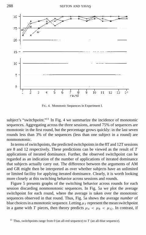
FIG. 4. Monotonic Sequences in Experiment I.

subject’s “switchpoint.”11 In Fig. 4 we summarize the incidence of monotonicsequences. Aggregating across the three sessions, around 75% of sequences aremonotonic in the first round, but the percentage grows quickly: in the last sevenrounds less than 3% of the sequences (less than one subject in a round) arenonmonotonic.

In terms of switchpoints, the predicted switchpoints in the 8T and 12T sessionsare 8 and 12 respectively. These predictions can be viewed as the result ofTapplications of iterated dominance. Further, the observed switchpoint can beregarded as an indication of the number of applications of iterated dominancethat subjects actually carry out. The difference between the arguments of AMand GR might then be interpreted as over whether subjects have an unlimitedor limited facility for applying iterated dominance. Clearly, it is worth lookingmore closely at this switching behavior across sessions and rounds.

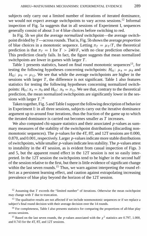
Figure 5 presents graphs of the switching behavior across rounds for eachsession discarding nonmonotonic sequences. In Fig. 5a we plot the averageswitchpoint for each round, where the average is taken over the monotonicsequences observed in that round. Thus, Fig. 5a shows the averagenumberofblue choices in a monotonic sequence. LettingµT represent the mean switchpointin a game withT pieces, then theory predictsµ4 < µ8 < µ12. In contrast, if

11 Thus, switchpoints range from 0 (an all-red sequence) toT (an all-blue sequence).


subjects only carry out a limited number of iterations of iterated dominance,we would not expect average switchpoints to vary across sessions.12 Informalinspection of Fig. 5a suggests that in all sessions of Experiment I, sequencesgenerally consist of about 3 or 4 blue choices before switching to red.

In Fig. 5b we plot the averagenormalizedswitchpoint—the average switch-point divided byT—across rounds. That is, Fig. 5b shows the averageproportionof blue choices in a monotonic sequence. LettingπT = µT /T , the theoreticalprediction is thatπT = 1 for T > 240/F , with no clear prediction otherwise.This prediction clearly fails. In fact, the figure suggests that mean normalizedswitchpoints are lower in games with largerT .

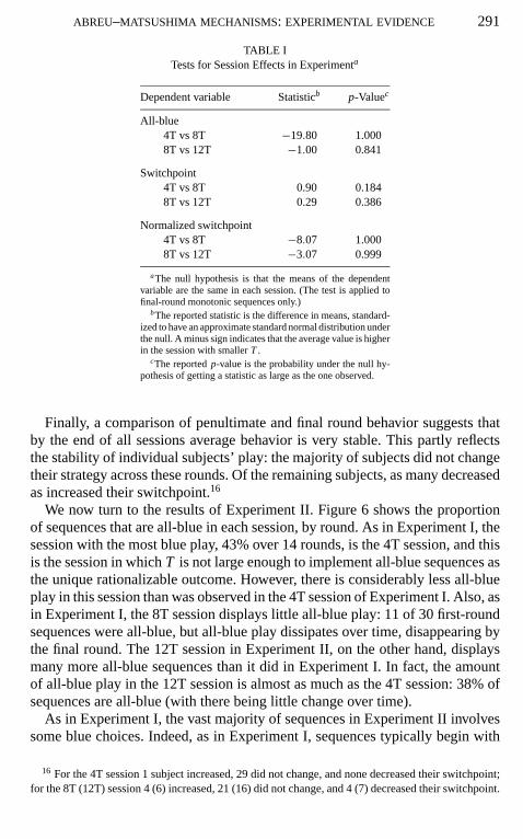
Table 1 presents statistics, based on final round monotonic sequences13, fortesting the following hypotheses concerning switchpoints:H01: µ4 = µ8 andH02: µ8 = µ12. We see that while the average switchpoints are higher in thesessions with largerT , the difference is not significant. Table 1 also featuresstatistics for testing the following hypotheses concerning normalized switch-points:H01:π4 = π8 andH02: π8 = π12. We see that, contrary to the theoreticalprediction, the mean normalized switchpoints are significantly lower in the ses-sions with largerT .14

Taken together, Fig. 5 and Table I support the following description of behaviorin Experiment I: in all three sessions, subjects carry out the iterative dominanceargument up to around four iterations, thus the fraction of the game up to whichthe iterated dominance is carried out becomes smaller asT increases.

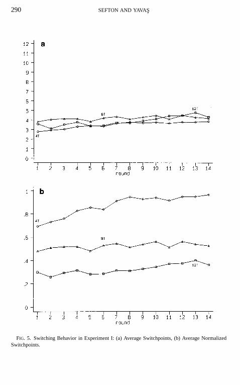
We also computed chi-square statistics and their associatedp-values as sum-mary measures of the stability of the switchpoint distributions (discarding non-monotonic sequences). Thep-values for the 4T, 8T, and 12T sessions are 0.000,0.870, and 0.001, respectively. Largerp-values indicate more stable distributionsof switchpoints, while smallerp-values indicate less stability. Thep-values attestto instability in the 4T session, as is evident from casual inspection of Figs. 3and 5, but the apparent round effect in the 12T session is not so easily inter-preted. In the 12T session the switchpoints tend to be higher in the second halfof the session relative to the first, but there is little evidence of significant changewithin the last seven rounds.15 Thus, we warn against interpreting the round ef-fect as a persistent learning effect, and caution against extrapolating increasingprevalence of blue play beyond the horizon of the 12T session.

12 Assuming thatT exceeds the “limited number” of iterations. Otherwise the mean switchpointmay change withT due to truncation.

13 The qualitative results are not affected if we include nonmonotonic sequences or if we replace asubject’s final round decision with their average decision over the 14 rounds.

14 For completeness, Table I also presents statistics for comparing the proportions of all-blue playacross sessions.

15 Based on the last seven rounds, thep-values associated with theχ2 statistics are 0.797, 1.000,and 0.743 for the 4T, 8T, and 12T sessions.


FIG. 5. Switching Behavior in Experiment I: (a) Average Switchpoints, (b) Average NormalizedSwitchpoints.


TABLE ITests for Session Effects in Experimenta

Dependent variable Statisticb p-Valuec

All-blue4T vs 8T −19.80 1.0008T vs 12T −1.00 0.841

Switchpoint4T vs 8T 0.90 0.1848T vs 12T 0.29 0.386

Normalized switchpoint4T vs 8T −8.07 1.0008T vs 12T −3.07 0.999

aThe null hypothesis is that the means of the dependentvariable are the same in each session. (The test is applied tofinal-round monotonic sequences only.)

bThe reported statistic is the difference in means, standard-ized to have an approximate standard normal distribution underthe null. A minus sign indicates that the average value is higherin the session with smallerT .

cThe reportedp-value is the probability under the null hy-pothesis of getting a statistic as large as the one observed.

Finally, a comparison of penultimate and final round behavior suggests thatby the end of all sessions average behavior is very stable. This partly reflectsthe stability of individual subjects’ play: the majority of subjects did not changetheir strategy across these rounds. Of the remaining subjects, as many decreasedas increased their switchpoint.16

We now turn to the results of Experiment II. Figure 6 shows the proportionof sequences that are all-blue in each session, by round. As in Experiment I, thesession with the most blue play, 43% over 14 rounds, is the 4T session, and thisis the session in whichT is not large enough to implement all-blue sequences asthe unique rationalizable outcome. However, there is considerably less all-blueplay in this session than was observed in the 4T session of Experiment I. Also, asin Experiment I, the 8T session displays little all-blue play: 11 of 30 first-roundsequences were all-blue, but all-blue play dissipates over time, disappearing bythe final round. The 12T session in Experiment II, on the other hand, displaysmany more all-blue sequences than it did in Experiment I. In fact, the amountof all-blue play in the 12T session is almost as much as the 4T session: 38% ofsequences are all-blue (with there being little change over time).

As in Experiment I, the vast majority of sequences in Experiment II involvessome blue choices. Indeed, as in Experiment I, sequences typically begin with

16 For the 4T session 1 subject increased, 29 did not change, and none decreased their switchpoint;for the 8T (12T) session 4 (6) increased, 21 (16) did not change, and 4 (7) decreased their switchpoint.


FIG. 6. All-Blue Play in Experiment II.

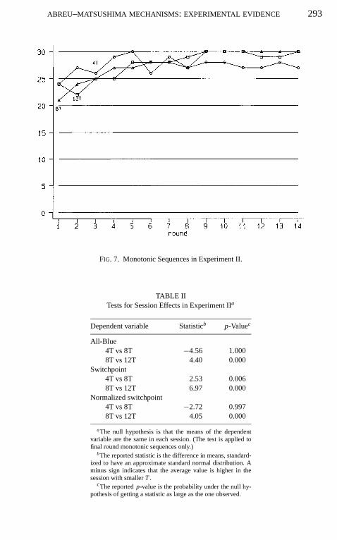
a blue choice and end with a red choice, switching from blue to red only once.Figure 7 summarizes the incidence of monotonic sequences in Experiment II,and is very similar to the corresponding figure for Experiment I. Around 25% ofsequences are nonmonotonic in the first round, but the percentage drops quicklyto less than 3% (less than one subject per round) in the last seven rounds.

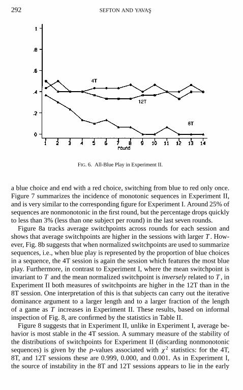
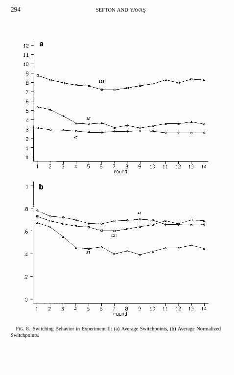
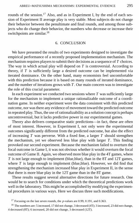
Figure 8a tracks average switchpoints across rounds for each session andshows that average switchpoints are higher in the sessions with largerT . How-ever, Fig. 8b suggests that when normalized switchpoints are used to summarizesequences, i.e., when blue play is represented by the proportion of blue choicesin a sequence, the 4T session is again the session which features the most blueplay. Furthermore, in contrast to Experiment I, where the mean switchpoint isinvariant toT and the mean normalized switchpoint isinverselyrelated toT , inExperiment II both measures of switchpoints are higher in the 12T than in the8T session. One interpretation of this is that subjects can carry out the iterativedominance argument to a larger length and to a larger fraction of the lengthof a game asT increases in Experiment II. These results, based on informalinspection of Fig. 8, are confirmed by the statistics in Table II.

Figure 8 suggests that in Experiment II, unlike in Experiment I, average be-havior is most stable in the 4T session. A summary measure of the stability ofthe distributions of switchpoints for Experiment II (discarding nonmonotonicsequences) is given by thep-values associated withχ2 statistics: for the 4T,8T, and 12T sessions these are 0.999, 0.000, and 0.001. As in Experiment I,the source of instability in the 8T and 12T sessions appears to lie in the early


FIG. 7. Monotonic Sequences in Experiment II.

TABLE IITests for Session Effects in Experiment IIa

Dependent variable Statisticb p-Valuec

All-Blue4T vs 8T −4.56 1.0008T vs 12T 4.40 0.000

Switchpoint4T vs 8T 2.53 0.0068T vs 12T 6.97 0.000

Normalized switchpoint4T vs 8T −2.72 0.9978T vs 12T 4.05 0.000

aThe null hypothesis is that the means of the dependentvariable are the same in each session. (The test is applied tofinal round monotonic sequences only.)

bThe reported statistic is the difference in means, standard-ized to have an approximate standard normal distribution. Aminus sign indicates that the average value is higher in thesession with smallerT .

cThe reportedp-value is the probability under the null hy-pothesis of getting a statistic as large as the one observed.


FIG. 8. Switching Behavior in Experiment II: (a) Average Switchpoints, (b) Average NormalizedSwitchpoints.


rounds of the session.17 Also, and as in Experiment I, by the end of each ses-sion of Experiment II average play is very stable. Most subjects do not changetheir behavior between the penultimate and final rounds, and among those sub-jects who do change their behavior, the numbers who decrease or increase theirswitchpoints are similar.18

6. CONCLUSION

We have presented the results of two experiments designed to investigate theempirical performance of a recently proposed implementation mechanism. Themechanism requires players to submit their decisions as a sequence ofT choices.The way in which actual play will depend onT is controversial. According totheory, if T is sufficiently large a desired outcome can be implemented viaiterated dominance. On the other hand, many economists feel uncomfortablewith this prediction because it is based on many rounds of iterated dominance,and the number of iterations grows withT . Our main concern was to investigatethe role of this crucial parameter.

In each experiment we conducted two sessions whereT was sufficiently largefor the mechanism to implement a unique rationalizable outcome of a coordi-nation game. In neither experiment were the data consistent with this predictedoutcome, nor was there any evidence of movement toward the predicted outcomein repeated play. Thus, the use of rationalizability as a solution concept is perhapsuncontroversial, but it lacks predictive power in our experimental games.

Theory also delivers comparative static predictions—in fact, these are oftenof most interest. However, in Experiment I, not only were the experimentaloutcomes significantly different from the predicted outcome, but also the effectof increasingT was perverse. With a fixed fine, a largerT should strengthenthe mechanism, yet we observed less blue play with largerT . This findingprovoked our second experiment. Because the mechanism failed to overturn thefocal outcome in Game I, it was not obvious whether it would overturn the focaloutcome of Game II. Again, we observed more blue play in the 4T games, whereT is not large enough to implement (blue,blue), than in the 8T and 12T games,whereT is large enough to implement (blue,blue). However, we did find thatstrengthening the mechanism increased blue play in Experiment II, in the sensethat there is more blue play in the 12T game than in the 8T game.

These results suggest several alternative directions for future research. Onewould be to search for conditions under which the theoretical predictions workwell in the laboratory. This might be accomplished by modifying the experimen-tal procedures in various ways. Here we discuss three such modifications.

17 Focusing on the last seven rounds, thep-values are 0.99, 0.191, and 0.363.18 The numbers are: 5 increased, 17 did not change, 3 decreased (4T); 3 increased, 23 did not change,

4 decreased (8T); 6 increased, 20 did not change, 3 decreased (12T).


First, AM argue that in any application the mechanism could be used togetherwith an explanation of how it works. This may help players appreciate the logicbehind the mechanism, and hence induce them to play as predicted. Our exper-iment does not include such an explanation, partly because we are concernedthat this might lead to changes in subject behavior that reflect their perceptionsabout what the experimenter wants them to do, regardless of any enhanced un-derstanding of the incentive structure of the game. Also, any explanation wouldhave to be incorporated into the experiment in a formal way, so that in principlethe same experimental procedures could be used by other researchers.

It should be noted that even if a player is enlightened by an explanation ofthe logic of the mechanism, the explanation would only be effective in inducingthe desired outcome in so far as the player believes other players are likewiseenlightened. Further, the explanation may be more or less persuasive, dependingon context. One can imagine a very persuasive explanation for Game II thatbegins with the sentence, “We will now explain how the fine can help you attainmaximum earnings, even though you will never have to pay the fine,” whereasthe same sentence is not available for Game I.

A second possible modification of the experiment might be to change thenature of repetition. We allowed subjects to learn about the game by having themplay repeatedly, but with changing partners. The performance of the mechanismmight be enhanced if partners were not rematched: if players best-respond to pastplay of their opponent, the unraveling that is supposed to take place at the levelof introspection may then take place over time, leading, ultimately, to all-blueplay. With changing partners, players get less information from opponents’ pastchoices, and this may inhibit unraveling. Of course, whether outcomes wouldchange in this way can be tested.19 The problem with unchanged pairings is thatit may introduce complicated repeated game effects, making interpretation ofthe outcomes difficult.

A third approach might be for the experimenter to increase the fine until themechanism works. The difference between the fine which is theoretically largeenough to induce the desired outcome and the effective fine could then be ameasure of “psychological barriers.” The outcome of this approach might be thedetermination of an excessively large effective fine: it may have to be so largeas to swamp other incentives. Also, our results from Game I suggest that theeffective fine for givenT may cease to be effective for larger values ofT .

An alternative direction for future research would be to explain the observeddiscrepancies between theory and evidence. We hope that our experiments canprovide some insights and suggestions for alternative theoretical models of theobserved behavior under the mechanism.

19 Andreoni (1988) finds that rematching has a small but statistically significant effect in a publicgood experiment.


APPENDIX: EXPERIMENTAL MATERIALS

This appendix contains materials for the Game I,T = 4 session. The other sessions included theobvious changes. Subject folders contained copies of the instructions, a record sheet and a decisionform.

Protocol

Upon entering the room, subjects are randomly seated. The door is closed after 30 subjects havebeen seated. They complete and return a consent form and are then given folders and the followingoral directions.

May I have your attention please. We are ready to begin. Thank you for coming. Each ofyou will be paid in cash at the end of the session. What you do during the session willdetermine how much.With the exception of the pencil and folder, please remove all materials from your desk.Open your folder, check that you have a set of instructions, a decision form, and a recordsheet inside. I will now read the instructions aloud. After the instructions have been readyou will have an opportunity to ask questions.

The experimenter reads the instructions.

Are there any questions?

At this stage there may be questions: The experimenter answers them by referring back to theinstructions if possible. If the question will be answered through the practice round, the experimentersays, “I think you’ll figure out the answer to that question when we go through the practice round, ifnot ask it again.”

If there are no questions, let’s begin the practice round. Circle your choices on the decisionform. Circle all four choices. And when you’ve made your choices, record them on yourrecord sheet. If anyone needs help raise your hand.You record your choices on line zero-a. Just write R for red and B for blue. You can’t fillout the other lines yet.When you’ve made your decision and recorded it, raise your hand so that a monitor cancome and get your decision form.

Monitors collect forms.

We won’t deliver the forms until everyone in both rooms has completed their decision.

Monitors deliver forms.

Now you should be receiving a form from the person in the other room that you’re pairedwith. Check you have the right form. Their number is at the top of the form and shouldmatch the number on your record sheet. Write their choices on row zero-b. Just use R forred and B for blue.

Monitors start circulating rooms, checking that subjects are doing it correctly.

This part is important. Record your earnings on line zero-c. Each time your choices matchyou get some points. Check the instructions if you don’t remember. If they don’t matchrecord a zero.Then figure out if you must subtract 90 points. If the first time you chose red was before orat the same time as the other person, subtract 90. If you need help raise your hand.To get your earnings for the round, add across line zero-c. Enter the total on the far right.The next round will count toward your earnings so it’s important to be straight on this now.

Monitors check calculations.


If there are no questions, we’ll close the screen and begin round one. The monitor will bringyou a decision form. Just put the used decision forms to one side.

Instructions

General Rules. This is an experiment in the economics of decision making. If you follow the instruc-tions carefully and make good decisions, you can earn a considerable amount of money. You will bepaid in private and in cash at the end of the experiment.

The experiment will consist of fifteen rounds, the first of which will be a practice round. The purposeof the practice round is to familiarize you with the experimental procedures. Nothing that you do inthe practice round will affect your earnings.

Notice that there are two rooms of subjects in this experiment. In each round you will be paired withanother person who is in the other room. You will never be paired with a person in your own room.You will be paired with a different person in each round. You will not know who is paired with you inany round. Similarly, the other people in this experiment will not know who they are paired with in anyround. To accomplish this, the partition between the two rooms will be closed before the beginning ofround one. It is important that you do not look at other peoples’ work, and that you do not talk, laughor exclaim out loud during the experiment. If you violate this rule you will be warned once. If youviolate this rule a second time you will be asked to leave and you will not be paid.

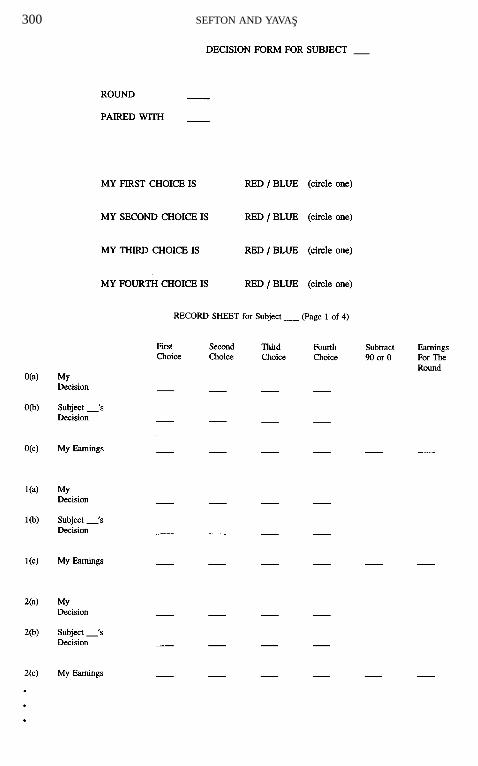
Description of Each Round. Each round consists of the following steps: (a) you will make a decisionand record it; (b) you will record the decision of the person you are paired with; and (c) you willcompute your earnings for the round. We will describe each step in turn.

(a) At the beginning of each round we will give you a “Decision Form.” The Decision Form for thepractice round (round zero) is in your folder. Look at it now. You make four choices in each round. Eachchoice is between “RED” and “BLUE”. You will enter your choices by circling the appropriate colorson the decision form. You will then copy your choices onto your “Record Sheet”. You will find thisrecord sheet in your folder. Look at it now. You will record your choices in round one on row 1(a). (Youwill record your choices in round two on row 2(a), and so on.) You will have three minutes to makeyour choices and record them. Then the monitor will collect your decision form. After the monitorshave collected all of the decision forms from both rooms, they will deliver your decision form to theperson in the other room with whom you are paired. They will also deliver to you the decision formcompleted by the person with whom you are paired.

(b) When you receive the decision form of the person you are paired with, you will record theirchoices on your record sheet. In round one, you will record their choices on row 1(b). (In round twoyou will record their choices on row 2(b), and so on.)

(c) You will then compute your earnings for the round according to rules we will discuss below andrecord them. In round one, you will record your earnings on row 1(c). (In round two you will recordyour earnings on row 2(c), and so on.) At the end of each round, you will record your earnings for thatround in the far right column of your record sheet. A monitor will record your earnings for that roundin the far right column of your record sheet. A monitor will check your calculations and, after everyonehas entered their earnings for the round correctly, the next round will begin.

How Your Earnings Are Determined. You will start the experiment with an initial balance of 1600points. This amount has already been entered in your record sheet. Your additional earnings in a roundwill depend on your choices and the choices of the person you are paired with. Your earnings from around will be determined as follows. If your first choice and the first choice of the person you are pairedwith are both “Red” you will each earn 120 points, if the first choices are both “Blue” you will eachearn 60 points, and if the first choices do not match (that is, if one of you chooses “Red” and the otherchooses “Blue”) you will each earn 0 points. Your earnings from the remaining three choices will bedetermined in exactly the same way. In each round you may also have to subtract 90 points from your


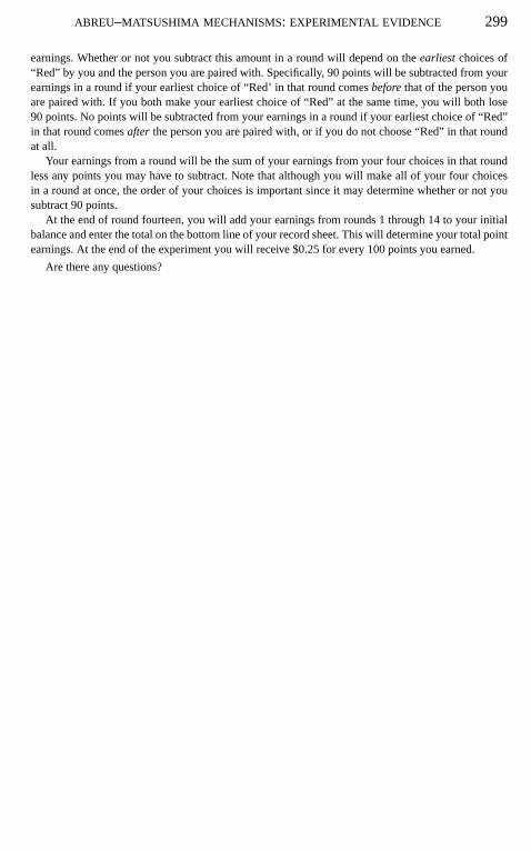
earnings. Whether or not you subtract this amount in a round will depend on theearliestchoices of“Red” by you and the person you are paired with. Specifically, 90 points will be subtracted from yourearnings in a round if your earliest choice of “Red’ in that round comesbeforethat of the person youare paired with. If you both make your earliest choice of “Red” at the same time, you will both lose90 points. No points will be subtracted from your earnings in a round if your earliest choice of “Red”in that round comesafter the person you are paired with, or if you do not choose “Red” in that roundat all.

Your earnings from a round will be the sum of your earnings from your four choices in that roundless any points you may have to subtract. Note that although you will make all of your four choicesin a round at once, the order of your choices is important since it may determine whether or not yousubtract 90 points.

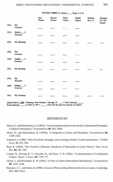
At the end of round fourteen, you will add your earnings from rounds 1 through 14 to your initialbalance and enter the total on the bottom line of your record sheet. This will determine your total pointearnings. At the end of the experiment you will receive $0.25 for every 100 points you earned.

Are there any questions?


REFERENCES

Abreu, D., and Matsushima, H. (1992a). “Virtual Implementation in Iteratively Undominated Strategies:Complete Information,”Econometrica60, 993–1008.

Abreu, D., and Matsushima, H. (1992b). “A Response to Glazer and Rosenthal,”Econometrica60,1439–1442.

Andreoni, J. (1988). “Why Free Ride? Strategies and Learning in Public Goods Experiments,”J. PublicEcon. 35, 291–304.

Basu, K. (1994). “The Traveler’s Dilemma: Paradoxes of Rationality in Game Theory,”Amer. Econ.Rev. 84, 391–395.

Cooper, R., DeJong, D. V., Forsythe, R., and Ross, T. W. (1992). “Communication in CoordinationGames,”Quart. J. Econ. 107, 739–771.

Glazer, J., and Rosenthal, R. W. (1992). “A Note on Abreu-Matsushima Mechanisms,”Econometrica60, 1435–1438.

Harsanyi, J. C., and Selten, R. (1988).A General Theory of Equilibrium Selection in Games. Cambridge,MA: MIT Press.


Kreps, D. M. (1990).A Course in Microeconomic Theory. Princeton, NJ: Princeton Univ. Press.

Sefton, M., and Yava¸s, A. (1995). “Risk and Coordination: Experimental Evidence,” Center for Nego-tiation and Conflict Resolution working paper. Penn State University.

Straub, P. G. (1995). “Risk Dominance and Coordination Failures in Static Games,”Quart. Rev. Econ.Finance35, 339–364.

Abreu Matsushima Mechanisms: Experimental Evidenceecon.ucsd.edu/~jandreon/Econ264/papers/Sefton...

Documents

Transcript of Abreu Matsushima Mechanisms: Experimental Evidenceecon.ucsd.edu/~jandreon/Econ264/papers/Sefton...