Abaqus Analysis Methods on Highly Restrained Pipeline with Soil Berm Formation

Shulong Liu*, Emil Maschner, Teng Zhang, John Smyth, John Li

Wood Group Kenny, Compass Point, 79-87 Kingston Road, Staines-upon-Thames, TW18

1DT, UK.

*Shulong.Liu@woodgroupkenny.com

Abstract: Wood Group Kenny has developed an advanced pipe-soil interaction subroutine to

accompany the analysis of pipeline lateral buckling and axial walking in Abaqus. The pipe-

soil interaction subroutine takes into consideration both variations in axial friction and the

lateral soil berm formation mechanism in the analysis of lateral buckling and axial walking of

pipelines subject to cyclic loading. The lateral soil berm formation scheme accounts for

differential berm growth on the soil berm front and rear faces, berm resistance accumulation,

mobilization distance and the residual ‘sweep’ friction variation in production operation

cycles. The subroutine monitors nodal displacement history around a buckle periphery, and

has been shown to simulate realistic, cyclic stress ranges, soil berm breakout mechanism

during rare high temperature /pressure loading events and the influence of lateral soil

restraint in global pipeline walking studies.

Due to the complexity of the berm formation mechanism, it has been found that small

differences in the initial lateral buckle profile generated using various Abaqus analysis

methods can have a significant impact during subsequent cyclic loading. This can be

important as it has the potential to alter the berm accumulation profile around the developing

lateral buckle; and more importantly impact on the pipeline behaviour with number of cycles.

Sensitivity checks, using various numerical analysis methods available to Abaqus users, to

identify the actual pipeline displacement behaviour in production operation cycles and

following mid-life or late life hot oiling events, are compared in this paper. A buckle

formation sensitivity check using various analysis methods, including static analysis with

stabilizer values, static analysis with various damping values, and the less-favoured static/

quasi dynamic analysis with RIKS method has been performed.

Keywords: Abaqus FEA, Pipe-Soil Interaction, Soil Berm Formation, Pipeline Lateral

Buckling, Cyclic Loading, Statics, Dynamics

1. Introduction

An on-bottom submarine pipeline system subject to high pressure and temperature loading is

susceptible to Euler buckling in the horizontal plane, i.e. lateral buckling, and indeed a

planned or controlled lateral buckle can be a safe and effective way to accommodate the

thermal expansion of a hot pipeline. However, as high stresses and strains can develop in such

buckles a simple stress based design approach will not suit the design of pipelines in

deepwater. Accordingly, within current oil and gas guidelines the conventional load limit

control maybe replaced by a strain limit control (SAFEBUCK III, 2011).

In theory, a single analysis of the entire pipeline could demonstrate that all failure modes will

be avoided, but in practice there are considerable uncertainties, including variable pipe-soil

interaction and as laid out-of-straightness that need to be taken into account. Thus choosing

one input to be conservative for one a failure mode can underestimate the effect of another.

The pipe-soil interaction model presented in SAFEBUCK III Design Guideline Appendix B,

most notably shows that lateral buckling, axial walking, route curve pull-out and flowline

anchoring are all extremely sensitive to the pipe-soil interaction forces. Consequently this

presents significant uncertainties to predicting the operational displacement response of

pipelines to ensure their through-life integrity.

In practice, analytical models may be used for simple configurations such as an exposed

pipeline on an even seabed and a buried pipeline. However, for more heavily loaded pipelines

on soft or uneven seabed with significant soil restraint advanced finite element methods are

required. Indeed industry codes and standards emphasis that lateral buckling in detailed design

of offshore pipelines must be modelled using a non-linear finite element method with quality

assurance and verification (DNV-RP-F110 2007, DNV OS F101 2013 and SAFEBUCK III

2011). Many commercial finite element analysis (FEA) packages are available, including

Abaqus, which has the capability to model snap buckling behaviour and the appropriate non-

linearity including non-linear geometry response, material non-linearity and non-linear elastic-

plastic pipe-soil interaction forces with user defined pipe-soil interaction subroutines. These

capabilities present Abaqus users with an opportunity to meet industry requirements in

running cost effective simulations involving variable complex input parameters to ensure the

operational displacement integrity of oil and gas pipelines.

There is still however a gap between the engineering needs of the oil and gas industry and

established engineering theory that has been written into many functions and subroutines

employed in FEA programs such as Abaqus. The oil industry is a fast growing sector, and

subsea oil field development needs state-of-art advanced simulation model with reliable and

accurate prediction that produces the right results first time. Wood Group Kenny has

developed a pipe-soil interaction subroutine (PSI), written in FORTRAN, that can be

embedded within an Abaqus global buckling FE model. The PSI subroutine has been

successfully validated for the analysis of advanced pipeline lateral buckling problems in

recent Wood Group Kenny projects.

The advanced pipe-soil interaction subroutine is to accompany pipeline lateral buckling and

axial walking analyses in Abaqus. The PSI subroutine takes into consideration both axial

friction variation and the lateral soil berm formation mechanism for pipeline lateral buckling

and walking analyses subject to production operation and pipeline service cyclic loadings. The

lateral soil berm formation takes into account differential berm growth on the soil berm front

and the rear faces, berm resistance accumulation and mobilisation distance and the residual

‘sweep’ friction variation in loading cycles. The subroutine can monitor nodal displacement

against its past displacement history around the buckle periphery. With regards to through life

oil and gas pipeline design the subroutine has been shown to simulate realistic, cyclic stress

ranges, soil berm breakout mechanism during rare high temperature /pressure loading events

and the influence lateral soil restraint in global pipeline walking studies.

Due to the complexity of the berm formation mechanism it has been found that small

differences in the initial lateral buckle profile generated using various Abaqus analysis

methods can have a significant impact during subsequent cyclic loading. This can be

important as it has the potential to alter the berm accumulation profile around the developing

lateral buckle and increasingly impact on the analysed pipeline behaviour with number of

cycles. To identify the actual pipeline displacement behaviour in production operation cycles

and following mid-life or late life hot oiling events, sensitivity checks using the various

numerical analysis methods available to Abaqus users are presented and compared in this

paper. The analysis methods employed for the buckle formation sensitivity checks include

static analysis with default ‘stabilize’ value, static analysis with specified ‘stabilize’ values,

static analysis with ‘direct damping factor’ values, static analysis employing RIKS method

and dynamic analysis.

Illustration of lateral buckle formation and soil berm development

To aide understanding Figures 1, 2 and 3 illustrate the typical soil berm formation process

occurring with cyclic start-up / shutdown operation (heat-up/cool-down). It should be noted

that the initial lateral buckle is formed as a consequence of pipeline out of straightness and

high pressure and temperature induced compression loading. The Figure 3 hysterisis plot

shows an initial soil breakout resistance to be overcome by the embedded pipe upon first

loading which results in the initial buckle formation.

Figure 1. Lateral buckle profiles seen during heat-up and cool-down

Figure 2. Continuum modelling of soil berm accumulation as a function of soil type, pipe weight, embedment and the extent of cyclic movement (S. Yu and I.

Konuk, 2007)

-2

-1

0

1

2

3

4

5

6

980 1000 1020 1040 1060 1080 1100 1120 1140 1160 1180

Late

ral D

isp

lace

men

t (m

)

Distance along pipeline (m)

Displaced pipe profile upon heat-up

Recovered pipe profile upon cool-down

Figure 3. Illustration of first load breakout during buckle formation and subsequent development on the advance and retreat pipe faces during cyclic

operation (SAFEBUCK III, 2011)

2. Methodology of the analysis

Pipeline global buckling and eventually local collapse of pipelines laid in deepwater seabed

can occur for a variety of reasons including excessive strain with associated stress/strain

concentration sites, fatigue, weld fracture aggravated by; high temperature, high pressure,

product slugging and the pipeline-seabed interaction. In this section, static analysis and

dynamic analysis methods suitable for global pipeline buckling and which are readily

available to Abaqus users and are reviewed (Abaqus User Manual).

Pipeline-soil interaction in production operation cycles is an important factor that can

dominate the pipeline fatigue and bending strain conditions. Results using the advanced Wood

Group Kenny pipe-soil interaction FORTRAN subroutine (PSI) are presented in this study.

2.1 Overview of the suitable analysis methods in Abaqus for global pipeline buckling

Results presented in the paper were generated as an outcome of an offshore subsea pipeline

design project completed by Wood Group Kenny, Detail comparison of the results obtained

using Abaqus with other commercially available FEA tools is outside the scope of this study,

and thus the effectiveness of this analysis method in other commercially available tools is not

reviewed.

Given the complexity of including inertial effects upon first loading a static stress analysis can

be used in Abaqus. In a static stress analysis time-dependent material effects such as creep,

swelling and viscoelasticity are ignored and conversely rate-dependent plasticity and

hysteretic behaviour for hyper-elastic materials can be taken into account.

To ensure as accurate and representative as possible results from FEA, a sensitivity study

employing adaptive automatic stabilisation with default stabilisation energy tolerance,

‘damping factor’ based on the dissipated energy fraction, ‘direct damping factor’ and RIKS

method has been performed. While the model is stable, viscous forces and, therefore, the

viscous energy dissipated are very small, thus, additional artificial damping has no effect. If a

local region becomes unstable the local velocities increase and, consequently, part of the strain

energy released is dissipated by the applied damping. The ‘damping factor’ is determined in

such a way that the dissipated energy for a given increment is a small fraction of the

extrapolated strain energy compared with the previous increment. The fraction is called the

dissipated energy fraction and, if a value is not specified by the user, a default value of 2.0 ×

10-4

is applied.

The RIKS method is generally used to predict unstable, geometrically nonlinear collapse of a

structure. For post buckling problems involving loss of contact (in this case the momentary

loss of contact between the pipelines and seabed as the pipeline buckles) the RIKS method

will usually not work unless inertia or viscous damping forces, such as those provided by

dashpots are introduced in a static or dynamic analysis to stabilize the solution.

The choice of appropriate method depends on the details of the analysis and the problem at

hand, below is a brief description of each of the methods available to Abaqus users (Abaqus

User Manual).

1. Adaptive automatic stabilization with the default stabilization energy tolerance in

static stress analysis

Adaptive automatic stabilisation with default stabilisation energy tolerance can be

defined in Abaqus using the following keywords:

*STATIC, STABILIZE

The default accuracy tolerance used by the adaptive automatic stabilisation scheme is

0.05. If the accuracy tolerance is not specified but a dissipated energy fraction with the

default value of 2.0 × 10-4

is used, the adaptive automatic damping algorithm will be

activated automatically with an accuracy tolerance of 0.05.

Whenever automatic stabilisation is used in a problem, the following criteria should be

checked to ensure that an accurate solution is obtained:

I. For a ‘damping factor’ calculated using the dissipated energy fraction it

necessary to check the factor to ensure that a reasonable amount of damping

has been applied.

II. Compare the viscous forces (VF) with the overall forces in the analysis and

ensure that the viscous forces are relatively small compared with the overall

forces in the model.

III. Compare the viscous damping energy (ALLSD) with the total strain energy

(ALLIE), and ensure that the ratio does not exceed the dissipated energy

fraction and adopts a reasonable value

IV. The ‘damping factor’ is neither too small, thus not controlling the

instability, or too large, thus leading to inaccurate results.

2. ‘Damping factor’ based on the dissipated energy fraction in static stress analysis

The non-default dissipated energy fraction for automatic stabilisation can be defined

directly using the following options:

*STATIC, STABILIZE=dissipated energy fraction

As mentioned, the ‘damping factor’ is determined using the dissipated energy fraction.

The ‘damping factor’ calculated from the dissipated energy for a given increment is a

small fraction of the extrapolated strain energy compared with the previous increment.

3. ‘Direct damping factor’ in static stress analysis

The ‘damping factor’ can be specified directly in the static analysis as follows:

*STATIC, STABILIZE, FACTOR=damping factor

A reasonable estimate for the ‘direct damping factor’ is generally quite difficult to make

unless a value is known from the output from previous runs. The ‘damping factor’

depends not only on the amount of damping but also on mesh size and material

behaviour. Unfortunately, there is no guarantee that the value of the chosen ‘damping

factor’ is optimal or even suitable in some cases.

During analysis it may, in some situations, be necessary to increase the ‘damping factor’

thus relaxing the convergence criteria if the system is unable to converge. Conversely it

may be necessary to decrease the ‘damping factor’ if a high ‘damping factor’ is

distorting the solution. The former would require the user to rerun the analysis with a

larger ‘damping factor’, while the latter would require the user to perform post-analysis

comparison of the energy dissipated by viscous damping to the total strain energy.

Therefore, obtaining an optimal value for the ‘damping factor’ is a manual process

requiring trial and error in the ‘direct damping factor’, until a converged solution is

obtained and the dissipated stabilisation energy is sufficiently small.

4. The RIKS method in static stress analysis

The RIKS method is generally used to predict unstable, geometrically nonlinear collapse

of a structure. It is often used to speed up the convergence of ill-conditioned or snap-

through problems that do not exhibit instability.

The RIKS algorithm cannot obtain a solution at a given load or displacement value since

these are treated as unknowns, rather the simulation terminates at the first solution that

satisfies the step termination criterion.

To obtain solutions at exact values of load or displacement, the solution must be restarted

at the desired point in the step and a new non-RIKS step must be defined. Since the

subsequent step is a continuation of the RIKS analysis, the load magnitude in that step

must be given appropriately so that the step begins with the loading continuing to

increase or decrease according to its behaviour at the point of restart. If a RIKS analysis

includes irreversible deformation such as plasticity, the point of restart should be ensured

to occur at a point in the analysis where the load magnitude is increasing if plasticity is

present.

As the pipeline buckles, a momentary to permanent loss of contact between the pipeline

and seabed surface take place, the RIKS method is not able to analyse this kind of

problem (SIMULIA Release Authorization and Stipulations, 2013). Consequently the

analysis of global pipeline buckling and post-buckling problems may not be so well

defined by the RIKS method.

5. Dynamic Analysis

Abaqus offers several methods for performing dynamic analysis of problems in which

inertia effects are considered. Dynamic analysis is outside the scope of this project;

hence it will not be discussed further in detail. However, for the benefit of the reader, a

transient dynamic analysis is defined using the keyword

*DYNAMIC

This option is used to provide direct integration of a dynamic stress/displacement

response in Abaqus and is generally used for nonlinear cases. The maximum time

increment allowed is the time period of the step divided by 100, including transient

analysis. Time period of the step and the loading history within the time step are found to

be critical issues for dynamic analysis of the pipeline global buckling. This is very

difficult to measure on site, and to be verified thereafter.

2.2 Soil berm formation verification

The berm formation mechanism is defined within the PSI subroutine in terms of berm

resistance, berm width in front and rear of the berm peak location (mobilisation distance) and

the mid-sweep resistance between the front and rear berms. Typically these cyclic soil berm

parameters are determined from field data and testing curves supplied by specialist

geotechnical consultancies. In certain less critical cases they can be approximated using the

methodology described in SAFEBUCK III.

Within the WGK sub-routine the parameters are calculated independently for the advance and

the retreat directions for individual nodal locations along the pipeline, and are functions of the

production cycle number (counted from the latest berm breakout in a given direction) and the

displacement of the pipeline between the berm in the front and the rear.

The berm strength, berm mobilisation and mid-sweep resistance are written into the PSI

subroutine as functions of both the cycle number and the displacement history using the

original measured data from laboratory. These functions which represent the berm data

sampled at different levels of cyclic displacement with number of cycles; say 5.0 diameters

(5D), 1.0 diameter (1D) and 0.1 diameters (0.1D) displacement. The mathematical curve fits

used in the WGK PSI subroutine presents a reasonable level of agreement with the original

supplied data.

As part of the validation process, a single element model and a full model are used to verify

that the berm response is adequately modelled by comparing the interpreted FE model and the

given curves. The results generally support the modelling scheme (Figures 4 to 6); however, it

appears that the berm mobilisation may lag the expected response by 1 cycle (Figure 6).

Whilst not believed to be critical it is considered that the 1 cycle lag may help to stabilise the

buckle growth slightly earlier and hence result in a slightly stronger berm under hot oil

conditions.

The berm resistance, mid-sweep resistance and the berm mobilisation curves are shown in

Figures 4 to 6. In Figures 4 through to 6, the displacement is unified to dimensionless by

dividing by the pipe diameter. The data points marked _Given are associated with the data

used in the PSI subroutine as an input for the FEA. The curves marked _FEA represent the

data generated in the Abaqus FE computational procedure from a user defined formula and

outputted from the Abaqus FE model.

Figure 4. Plot of showing the variation in berm resistance with pipeline sweep distance and cycle number

Figure 5. Plot of showing the variation of the mid-sweep residual resistance with pipeline sweep distance and cycle

Figure 6. Plot showing the variation in the berm mobilization distance with pipeline sweep distance and cycle number

Figure 7 illustrates at the apex of a lateral buckle the cyclic build-up of soil berm friction in

the first 20 cycles of operation. As can be seen from initial buckle formation (cycle 0) the

buckle profile continues to grow for some 11 cycles of heat-up / cool-down operation

continuously breaking out of the small soil berm on each heating step. From cycle 11 the

buckle form ceases to grow further in the advance direction enabling the soil berm to develop

with subsequent cycles. The cyclic displacement pattern and the lateral reaction of the pipe

against the accumulated soil berm resistance at the buckle apex are also shown in Figure 7.

The theory and pipeline engineering associated with the Wood Group Kenny pipe-soil

interaction simulation subroutine is outside the scope of this paper, and consequently detailed

discussion of the development methodology of the subroutine is will not be presented here.

Figure 7. Typical results plot at the apex of a lateral buckle showing the pipe

reaction against accumulated soil berm resistance and cyclic displacement.

3. Results from the analysis

Given the problem at hand and after reviewing the suitability of each of the built-in Abaqus

analysis methods for analysing global buckling of offshore pipelines (refer to Abaqus User

Manual), the static analysis with damping based on the dissipated energy fraction was used to

achieve the project deliverables. The other methods discussed earlier in the paper are

employed in this study as a sensitivity check.

In this study, initial concerns arose over different post hot-oil results seen from cases with

similar first load responses. To illustrate the effect of the different Abaqus analysis methods

on the results of pipeline global buckling analysis, a 10” pipeline on a flat seabed with a VAS

length of 2160m and an initial imperfection of 1m at the planned buckle apex is used. The

pipeline lateral profile is established in first production (first load), this initial profile will be

further stabilized in production heat-up and cool-down operation cycles. After 20 cycles of

normal production operation, the pipeline will be serviced with hot oil causing it to push into

the yielding soil berm and impose high bending strain on the pipeline.

The uses of the analysis methods, i.e. either static or dynamic, vary only in the first production

operation. The effect of each of the analysis methods is expected to be isolated in the first

production operation and then subsequently the effect of the various methods is propagated to

the hot oiling step through the 20 production operation cycles. In pipeline analysis, the

minimum and maximum strains are calculated and compared at all the peripheral integration

points on elements at various locations along the pipeline. Note that along the pipeline the

minimum strain is not necessarily a compressive strain and the maximum strain is not

necessarily a tensile strain, however for convenience, in this paper, the minimum strain is

termed the maximum compressive strain and the maximum strain is termed the maximum

tensile strain. The strain value at the buckle apex refers to the longitudinal maximum

tensile/compressive component of mechanical strain along the pipeline axial direction, unless

otherwise stated.

3.1 Sensitivity check of the ‘stabilize’ value in static analysis

Results presented in this section demonstrate the effect of the ‘stabilize’ values in Abaqus

static analysis for the prediction of pipeline behaviour in production operation and during

service. The static analysis at first load is set with the adaptive automatic stabilisation, for all

other cases the ‘stabilize’ function takes values ranging from 10-1

to 10-10

.The adaptive

automatic dissipated energy fraction is set adopt a default ‘stabilize’ value of 2×10-4

in

Abaqus static analysis (refer to Abaqus User Manual). Results from this case are used, in this

study, as the base case and labelled as DEFAULT.

The effect of varying the ‘stabilize’ value from 10-1

to 10-10

on the lateral displacement and the

maximum compressive strain at buckle apex are summarised in Table 1. It should be noted

that the percentage difference presented in Table 1 and subsequent tables represents the result

(e.g. the displacement at the buckle apex) under a specific condition compared with the

equivalent from the base case (which takes a ‘stabilize’ value of 2×10-4

).

Table 1. Sensitivity check when varying the ‘stabilize’ value in static analysis (displacement at the buckle apex)

‘Stabilize’ Value First Load Diff% Cycle 20 Diff% Hot Oiling Diff%

1E-10 4.84 -1% 6.42 1% 8.32 -2%

1E-07 4.75 -3% 6.22 -2% 8.54 1%

1E-05 4.87 -1% 6.28 -1% 8.50 1%

Default (2E-04) 4.91 0% 6.37 0% 8.45 0%

1E-03 4.94 1% 6.59 3% 8.69 3%

1E-02 4.97 1% 6.36 0% 8.72 3%

1E-01 4.82 -2% 6.31 -1% 8.56 1%

Table 2. Sensitivity check when varying the ‘stabilize’ value in static analysis (maximum compressive mechanical strain at buckle apex)

‘Stabilize’ Value First Load Diff% Cycle 20 Diff% Hot Oiling Diff%

1E-10 -0.279% -1% -0.213% -2% -0.414% -31%

1E-07 -0.276% -2% -0.197% -10% -0.386% -36%

1E-05 -0.282% 0% -0.210% -4% -0.516% -14%

Default (2E-04) -0.281% 0% -0.218% 0% -0.600% 0%

1E-03 -0.285% 1% -0.214% -2% -0.362% -40%

1E-02 -0.283% 1% -0.205% -6% -0.384% -36%

1E-01 -0.271% -4% -0.195% -11% -0.351% -42%

Figure 8 shows a plot of the displacements at the buckle apex presented in Table 1, the x-axis

adopts a logarithmic scale, lg(X). Table 1 and Figure 8 show that when varying the ‘stabilize’

value from 10-1

to 10-10

, the lateral displacement at the buckle apex varies by 3% when

compared with the default setting in all the presented pipeline production operation and

pipeline service steps. The percentage difference of 3% in the lateral displacement at the

buckle apex results in up to percentage differences of 4%, 11% and 42% in the longitudinal

mechanical compressive strain in the first production operation, production operation cycle 20

and the hot oiling step, respectively.

Figure 8. Sensitivity check when varying the ‘stabilize’ value in static analysis (displacement at buckle apex)

Figure 9. Sensitivity check when varying the ‘stabilize’ value in static analysis (mechanical strain at buckle apex)

The results for the hot oiling step illustrated in Figure 9 show that as far as the maximum

longitudinal compressive mechanical strain is concerned in the analysis, the choice of the

‘stabilize’ value and the associated sensitivity check becomes very important in the analysis of

4

4.5

5

5.5

6

6.5

7

7.5

8

8.5

9

-10 -8 -6 -4 -2

Dis

pla

cem

en

t (m

)

Common Logarithm of the Dissipated Energy Fraction (lg(x))

Sensitivity Check of the Dissipated Energy Fraction (Stabilize Value) in Static Analysis

First Production Cycle 20 Hot Oiling

-0.6%

-0.5%

-0.4%

-0.3%

-0.2%

-0.1%

-10 -9 -8 -7 -6 -5 -4 -3 -2 -1

Lon

gitu

din

al S

trai

n C

om

po

ne

nt

(%)

Common Logarithm of the Dissipated Energy Fraction (lg(x))

Sensitivity Check of the Dissipated Energy Fraction in Static Analysis

First Production Cycle 20 Hot Oiling

pipeline global buckling subject to production operation cycles and further high temperature

events.

The pipeline lateral displacement profiles and the maximum tensile strain profiles along the

pipeline in the buckle region at first production, production cycle 20 and the hot oiling step as

varying ‘stabilize’ values using Abaqus static analysis are illustrated and compared in Figures

10 and 11. Prod, C20 and Oil are used to denote the results from the first production,

production cycle 20 and the hot oiling cases, respectively. This notation coupled with 1E_3

and 1E_5 represent the results from each respective case with ‘stabilize’ values of 10-3

and 10-

5, respectively.

Figure 10. ‘Stabilize’ value sensitivity check in static analysis (pipeline ½ lateral profiles)

-2

0

2

4

6

8

10

980 1000 1020 1040 1060 1080

Late

ral D

isp

lace

me

nt

(m)

Pipe Length (m)

Stabilize Value (Energy Dissipation Fraction) Sensitivity Check

Prod_Stabilize_1E-3 Prod_Default Prod_Stabilize_1E-5C20_Stabilize_1E-3 C20_Default C20_Stabilize_1E-5Oil_Stabilize_1E-3 Oil_Default Oil_Stabilize_1E-5

Figure 11. ‘Stabilize’ value sensitivity check in static analysis (maximum tensile strain profile)

Figures 10 and 11 show that at the first production load step and production cycle 20, both the

pipeline lateral profiles and maximum longitudinal tensile strain component profiles have

good agreement along the pipeline length in the buckle region when varying the ‘stabilize’

values. In the hot oiling step the pipeline lateral profiles show a reasonable good level of

agreement, with varying ‘stabilize’ values. However, the maximum longitudinal tensile strain

component profiles are almost identical away from the buckle crown, but largely have

deviated at the narrow buckle crown region from about 0.32% to 0.52%.

Under the hot oiling condition, a content temperature of 83˚C is assumed. As a higher

temperature event is encountered, the gap of the predicted strain values may be magnified,

suggesting that a temperature sensitivity check is needed to identify the effect of temperature

in conjugation with varying the ‘stabilize’ value in the analysis of pipeline in deepwater

subject to high temperature and high pressure.

3.2 Sensitivity check of the ‘direct damping factor’ in static analysis.

The effect of the ‘direct damping factor’ in Abaqus static analysis has been examined directly

by varying the damp factor value from 10-1

to 10-8

.

Tables 3 and 4 summarise the lateral displacement and the maximum compressive strain at the

buckle apex in first production, production cycle 20 and hot oiling steps, with the ‘damping

factor’ value varying from 10-1

to 10-8

.

Table 3. Sensitivity check when varying ‘damping factor’ in static analysis (lateral displacement at buckle apex)

‘Damping factor’ Value First Load Diff% Cycle 20 Diff% Hot Oiling Diff%

1E-08 4.21 -14% 6.56 3% 8.56 1%

1E-07 4.74 -3% 6.64 4% 8.49 0%

1E-06 4.78 -3% 6.69 5% 8.64 2%

1E-05 4.81 -2% 6.23 -2% 8.09 -4%

1E-04 4.78 -3% 6.30 -1% 8.31 -2%

-0.1%

0.0%

0.1%

0.2%

0.3%

0.4%

0.5%

0.6%

980 1000 1020 1040 1060 1080Max

. Lo

ngi

tud

inal

Me

chan

ical

Str

ain

(%

)

Pipeline Length (m)

Satbilize Value (Energy Dissipation Fraction) Sensitivity Check

Prod_Max_1E-3 Prod_Max_Default Prod_Max_1E-5C20_Max_1E-3 C20_Max_Default C20_Max_1E-5Oil_Max_1E-3 Oil_Max_Default Oil_Max_1E-5

1E-03 4.74 -3% 6.57 3% 8.51 1%

1E-02 4.68 -5% 6.17 -3% 8.00 -5%

1E-01 4.49 -9% 6.14 -4% 7.93 -6%

Table 4. Sensitivity check when varying ‘damping factor’ in static analysis (longitudinal maximum mechanical strain at buckle apex)

‘Damping factor’ Value First Load Diff% Cycle 20 Diff% Hot Oiling Diff%

1E-08 -0.267% -5% -0.233% 7% -0.374% -38%

1E-07 -0.273% -3% -0.223% 2% -0.378% -37%

1E-06 -0.279% -1% -0.229% 5% -0.388% -35%

1E-05 -0.279% -1% -0.205% -6% -0.552% -8%

1E-04 -0.275% -2% -0.199% -9% -0.414% -31%

1E-03 -0.275% -2% -0.221% 1% -0.370% -38%

1E-02 -0.274% -2% -0.193% -11% -0.417% -31%

1E-01 -0.283% 1% -0.213% -2% -0.456% -24%

The results presented in Table 3 shows that when varying the ‘damping factor’ values ranging

from 10-1

to 10-8

, the lateral displacement at the buckle apex varies with maximum values of

14%, 5% and 6% when compared with the base case for the first load, cycle 20 and the hot

oiling steps, respectively.

From Table 4 it is observed that the longitudinal maximum compressive mechanical strain at

the buckle apex varies up to 5% and 11% when compared with the base case first load, cycle

20 steps respectively. A percentage difference of less than 6% in lateral displacement, results

in up to 38% percentage difference in the longitudinal mechanical compressive strain in the in

the hot oiling step.

Figures 12 and 13 show plots of the lateral displacement and the maximum compressive strain

at the buckle apex displayed in Tables 3 and 4.

Figure 12. Sensitivity check when varying ‘damping factor’ in static analysis (lateral displacement at apex)

4

4.5

5

5.5

6

6.5

7

7.5

8

8.5

9

-8 -7 -6 -5 -4 -3 -2 -1

Dis

pla

cem

en

t (m

)

Common Logarithm of the Damping Factor (lg(x))

Sensitivity Check of the Direct Damping Factor in Static Analysis

First Production Cycle 20 Hot Oiling

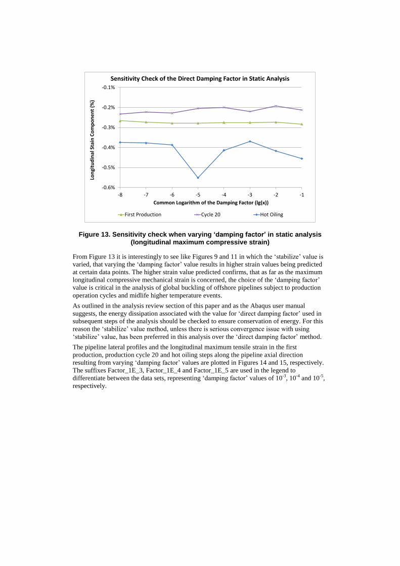
Figure 13. Sensitivity check when varying ‘damping factor’ in static analysis (longitudinal maximum compressive strain)

From Figure 13 it is interestingly to see like Figures 9 and 11 in which the ‘stabilize’ value is

varied, that varying the ‘damping factor’ value results in higher strain values being predicted

at certain data points. The higher strain value predicted confirms, that as far as the maximum

longitudinal compressive mechanical strain is concerned, the choice of the ‘damping factor’

value is critical in the analysis of global buckling of offshore pipelines subject to production

operation cycles and midlife higher temperature events.

As outlined in the analysis review section of this paper and as the Abaqus user manual

suggests, the energy dissipation associated with the value for ‘direct damping factor’ used in

subsequent steps of the analysis should be checked to ensure conservation of energy. For this

reason the ‘stabilize’ value method, unless there is serious convergence issue with using

‘stabilize’ value, has been preferred in this analysis over the ‘direct damping factor’ method.

The pipeline lateral profiles and the longitudinal maximum tensile strain in the first

production, production cycle 20 and hot oiling steps along the pipeline axial direction

resulting from varying ‘damping factor’ values are plotted in Figures 14 and 15, respectively.

The suffixes Factor_1E_3, Factor_1E_4 and Factor_1E_5 are used in the legend to

differentiate between the data sets, representing ‘damping factor’ values of 10-3

, 10-4

and 10-5

,

respectively.

-0.6%

-0.5%

-0.4%

-0.3%

-0.2%

-0.1%

-8 -7 -6 -5 -4 -3 -2 -1

Lon

gitu

din

al S

tain

Co

mp

on

en

t (%

)

Common Logarithm of the Damping Factor (lg(x))

Sensitivity Check of the Direct Damping Factor in Static Analysis

First Production Cycle 20 Hot Oiling

Figure 14. Sensitivity check when varying ‘damping factor’ (Pipeline ½ lateral profile)

Figure 15. Sensitivity check when varying ‘damping factor’ (maximum tensile strain profile)

The results presented in Figure 14 and 15 illustrate that for the first production load step and

the production cycle 20, both the pipeline lateral profiles and maximum longitudinal tensile

strain component profiles have good agreement under the varying ‘damping factor’ values.

The results generated for the hot oiling step show that the pipeline lateral profiles have

reasonable good agreements in general under directly varying the ‘damping factor ' values.

-2

0

2

4

6

8

10

980 1000 1020 1040 1060 1080

Late

ral D

isp

lace

me

nt

(m)

Pipe Length (m)

Direct Damping Factor Value Sensitivity Check

Prod_Factor_1E-3 Prod_Factor_1E-4 Prod_Factor_1E-5C20_Factor_1E-3 C20_Factor_1E-4 C20_Factor_1E-5Oil_Factor_1E-3 Oil_Factor_1E-4 Oil_Factor_1E-5

-0.1%

0.0%

0.1%

0.2%

0.3%

0.4%

0.5%

0.6%

980 1000 1020 1040 1060 1080Max

. Lo

ngi

tud

inal

Me

chan

ical

Str

ain

(%

)

Pipeline Length (m)

Direct Damping Factor Value Sensitivity Check

Prod_Max_1E-3 Prod_Max_1E-4 Prod_Max_1E-5C20_Max_1E-3 C20_Max_1E-4 C20_Max_1E-5

Oil_Max_1E-3 Oil_Max_1E-4 Oil_Max_1E-5

Interestingly, the maximum longitudinal tensile strain component profiles are almost identical

away from the primary buckle region, but have largely deviated at the buckle crown narrow

region from approximately 0.32% to 0.52%.

3.3 Effect of the analysis methods

In addition to the Abaqus analysis methods outlined earlier a first load analysis employing the

RIKS method and a dynamic analysis, was undertaken. The initial first load buckle profiles

were seen to exert a significant impact on final hot oil strains following cyclic analyses. The

20 cycle operation displacements and strains and the subsequent hot oil displacements and

strains are presented in Tables 5 and 6.

It is common practice, in global pipeline buckling analysis, that a stabilize value of around 10-

4 and a ‘damping factor’ value of around 10

-3 be used. These values are favoured so as to

achieve a reasonable balance between the computational time (and its associated cost!) and the

user accuracy requirement. To increase comparability between the results under the different

cases analysed, a ‘stabilize’ value of 2×10-4

(base case) and a ‘damping factor’ value of

around 10-3

are used to compare results with results emerging from RIKS method and

dynamic analyses.

As mentioned earlier, in RIKS analysis, the exact results cannot be achieved directly in its

own step. Rather a non-RIKS step in the first production is used to continue the RIKS step to

achieve the results under a specified load condition. In the first production operation, a non-

RIKS step has been used to continue a RIKS run under two scenarios, the first being a non-

RIKS step is used to continue a RIKS step before the RIKS run reached a peak on the

monotone increasing stress-strain curve, and in the other on the peak of the monotone

increasing stress-strain curve. These are labelled RIKS1 and RIKS

2 respectively in Tables 5

and 6. These two scenarios have been considered to check the reliability of results generated

when a RIKS step is manually continued by a non-RIKS analysis step analysis. It should be

noted that, if a non-RIKS step is used to continue a RIKS step to early on the monotone

increasing stress-strain curve, the advantages of RIKS analysis may not be accurately of

sufficiently portrayed. Conversely, if a non-RIKS step is used to continue a RIKS step too far

along the monotone increasing stress-strain curve, the results might be distorted when there is

large plasticity in the RIKS analysis step.

Figure 16 compares both RIKS generated buckle profiles against the lateral profile generated

using the project ‘Stabilize’ value with an initial 1m out of straightness. As can be seen the

RIKS method generates lateral profiles of larger amplitude than with the Abaqus ‘Stabilize’

method with shallower secondary lobes. As seen in Table 6 the initial RIKS profiles carried

through 20 cycles of operation can give rise to significant differences in the final berm

breakout strain levels.

Figure 17 illustrates that the choice of initial pipeline out of straightness in buckle formation

sensitivity analyses can also give rise to different initial buckle profiles impacting on final

strain levels. The comparative FE runs without system damping using another FE package

shows smaller levels of initial out of straightness giving rise to more dynamic buckle

developments tend towards the RIKS profiles whilst larger 1m out of straight imperfections

develop the prominent secondary lobes seen using the Abaqus ‘Stabilise’ value.

Figure 16. Variation seen in initial first load and 20 cycle hot oil buckle profiles using RIKS

1&2 and default ‘Stabilize’ parameters

Figure 17. Un-damped first load buckle profiles seen with different levels of initial pipeline out of straightness

Note that the smaller more dynamic buckle form generated with lower 0.2m levels of initial

OOS compares more closely with Abaqus RIKS simulations undertaken with 1m initial OOS.

The lateral displacement and the maximum compressive strain component values at the

planned buckle apex are shown in Tables 5 and 6.

Table 5. Effect of the Abaqus analysis methods to predicted lateral displacement at apex

Method First Load Diff% Cycle 20 Diff% Hot Oiling Diff%

-2

0

2

4

6

8

10

980 1000 1020 1040 1060 1080 1100 1120 1140 1160 1180

Late

ral D

isp

lace

me

nt

(m)

Pipe Length (m)

Default_Prod RIKS1_Prod RIKS2_Prod

Default_Oiling RIKS1_Oiling RIKS2_Oiling

-2

-1

0

1

2

3

4

5

6

980 1000 1020 1040 1060 1080 1100 1120 1140 1160 1180

Late

ral d

ispl

acem

ent (

m)

Distance along pipe (m)

1m x 100m OOS

0.2m x 200m OOS

Default Stabilize (2×10-4) 4.91 0% 6.37 0% 8.45 0%

‘Damping factor’ (1×10-3) 4.74 -3% 6.57 3% 8.51 1%

RIKS1 5.61 14% 6.90 8% 9.07 7%

RIKS2 6.84 39% 6.65 4% 8.31 -2%

Dynamic 6.10 24% 6.02 -5% 6.72 -20%

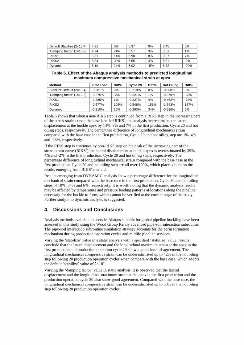
Table 6. Effect of the Abaqus analysis methods to predicted longitudinal maximum compressive mechanical strain at apex

Method First Load Diff% Cycle 20 Diff% Hot Oiling Diff%

Stabilize Default (2×10-4) -0.281% 0% -0.218% 0% -0.600% 0%

‘Damping factor’ (1×10-3) -0.275% -2% -0.221% 1% -0.370% -38%

RIKS1 -0.285% 1% -0.227% 4% -0.462% -23%

RIKS2 -0.577% 105% -0.548% 151% -1.543% 157%

Dynamic -0.310% 10% -0.293% 34% -0.636% 6%

Table 5 shows that when a non-RIKS step is continued from a RIKS step in the increasing part

of the stress-strain curve, the case labelled RIKS1, the analysis overestimates the lateral

displacement at the buckle apex by 14%, 8% and 7% in the first production, Cycle 20 and hot

oiling steps, respectively. The percentage difference of longitudinal mechanical strain

compared with the base case in the first production, Cycle 20 and hot oiling step are 1%, 4%

and -23%, respectively.

If the RIKS step is continues by non-RIKS step on the peak of the increasing part of the

stress-strain curve (RIKS2) the lateral displacement at buckle apex is overestimated by 39%,

4% and -2% in the first production, Cycle 20 and hot oiling steps, respectively. The

percentage difference of longitudinal mechanical strain compared with the base case in the

first production, Cycle 20 and hot oiling step are all over 100%, which places doubt on the

results emerging from RIKS2 method.

Results emerging from DYNAMIC analysis show a percentage difference for the longitudinal

mechanical strain compared with the base case in the first production, Cycle 20 and hot oiling

steps of 10%, 34% and 6%, respectively. It is worth noting that the dynamic analysis results

may be affected by temperature and pressure loading patterns at locations along the pipeline

necessary for the buckle to form, which cannot be verified at the current stage of the study.

Further study into dynamic analysis is suggested.

4. Discussions and Conclusions

Analysis methods available to users in Abaqus suitable for global pipeline buckling have been

assessed in this study using the Wood Group Kenny advanced pipe-soil interaction subroutine.

The pipe-soil interaction subroutine simulation strategy accounts for the berm formation

mechanism during production operation cycles and midlife pipeline services.

Varying the ‘stabilize’ value in a static analysis with a specified ‘stabilize’ value, results

conclude that the lateral displacement and the longitudinal maximum strain at the apex in the

first production and production operation cycle 20 show a good level of agreement. The

longitudinal mechanical compressive strain can be underestimated up to 42% in the hot oiling

step following 20 production operation cycles when compare with the base case, which adopts

the default ‘stabilize’ value of 2×10-4

.

Varying the ‘damping factor’ value in static analysis, it is observed that the lateral

displacement and the longitudinal maximum strain at the apex in the first production and the

production operation cycle 20 also show good agreement. Compared with the base case, the

longitudinal mechanical compressive strain can be underestimated up to 38% in the hot oiling

step following 20 production operation cycles.

Static analysis with RIKS method showed convergence issues, this is likely to be due to the

momentary or permanent loss of surface contact between pipeline and soil surfaces when a

buckle occurs. The computational runs using RIKS method have been conducted by a trial and

error procedure. The quality of the predicted results may rely on a good educated guess of the

point on the monotone increasing stress-strain curve where a non-RIKS step should continue

the RIKS step.

The pipeline lateral profile from the dynamic analysis failed to present good agreement with

the equivalent results emerging from a static analysis. Further study to understand the global

buckling dynamic behaviour of pipelines in deepwater subject to high temperature and high

pressure events is much needed, especially as the complexity of offshore pipeline projects is

ever increasing.

Motivation for this study and subsequently the development of the PSI subroutine was

triggered by concerns expressed over different post hot-oil results seen from cases started with

rather similar first load responses. The large differences in analysis results under hot oiling

may indicate that a good quality berm formation strategy is need, for projects related to the oil

and gas industry. The subroutine presented in this paper is one such solution.

The accumulated difference in cyclic analyses resulting from using inappropriate Abaqus

analysis methods at the first load step may result in differences in the berm formation. As the

pipeline is fully locked-in to the soil berm, the berm resistance experienced by the pipeline

may not actually be the available berm resistance. The difference in berm formation resulting

from a cumulative error as an outcome of using a certain analysis method may not be

immediately apparent to the user. In hot oiling events, the pipeline buckle crown further

breaks out from the berm and may meet and have to overcome the diverged cumulated berm

surrounding the pipeline.

This study has highlighted the need for using advanced pipe-soil interaction model to account

for the berm formation mechanism in deepwater environment related to the oil and gas

industry. The development and subsequent validation of the Wood Group Kenny advanced

pipe-soil interaction subroutine in recent projects has offered opportunity to look into this

phenomenon, the detailed theory and development methodology of this subroutine will be

reported in due course in a further publication.

5. Acknowledgements

This study was carried out under the support of Wood Group Kenny at Aberdeen and London

offices in UK, Galway office in Republic of Ireland and Melbourne office in Australia, which

is appreciated. Special thanks to Dr. Mahmoud H. M. Ahmed for his contribution in finalising

the paper manuscript.

6. References

1. ABAQUS User’s Manual, Version 6.12, SIMULIA, Dassault Systèmes Simulia

Corp., 2012.

2. SIMULIA Release Authorization and Stipulations, Dassault Systèmes Simulia Corp,

September 3, 2013.

3. Safe Design of Pipeline with Lateral Buckling Design Guideline, SAFEBUCK III

5087471/01/A, 2011.

4. Global Buckling of Submarine Pipelines, DNV Offshore Codes Recommended

Practice DNV-RP-F110, Det Norske Veritas, 2007.

5. Submarine Pipeline Systems, Offshore Standard DNV-OS-F101, Det Norske Veritas,

2013.

6. E.J. Chin, D. Scholtz, E. Shim, E. Gerginov, “The Effects of Soil Berm Formation on

Pipeline Fatigue Response at Buckle sites” Deep Offshore Technology (DOT)

International Conference, Houston, Texas USA, 2013

7. S. Yu and I. Konuk, “Continuum FE modelling of lateral buckling” OTC 18934,

2007.