A workflow to account for uncertainty in well-log data in ... in 3D geostatistical reservoir...
32
A workflow to account for uncertainty in well-log data in 3D geostatistical reservoir modeling Jose Akamine and Jef Caers May, 2007 Stanford Center for Reservoir Forecasting Abstract Traditionally well log data is used as hard data in reservoir modeling using geosta- tistics; this means that we apply a constraint that needs to be honored exactly by the reservoir model. But if we know that a log is not reliable because of the log quality then the model will be constrained by non-reliable data. One could then argue in more general terms that in most practical cases hard data on either facies or petrophysical properties does not exist because well log data requires processing and interpretation before reaching the geostatistical modeling stage. The traditional method approach using Kriging with error variance assumes that the reservoir modeler knows the error covariance and assumes it is uncorrelated. An- other traditional approach, the Bayesian modeling, assumes Gaussianity because the likelihood of the error model cannot be easily obtained. In order to overcome these limitations a data pre-posterior iterative algorithm approach is proposed. Several real- izations of the uncertain well log data are generated taking into account the reliability of the well log measurements and they serve as input for the reservoir modeler to loosen the well constraints while at the same time honoring the geological spatial continuity. We present an application of this workflow to a real reservoir case study. 1 Introduction In stochastic modeling, one aims at creating several realizations of some true spatial phe- nomenon. These realizations are constrained to a variety of data, typically categorized in hard data versus soft data. Soft data are data that provide indirect information about the primary variable under investigation. Soft data are measurements of a secondary variable that is related to the primary variable. Hard data are direct measurements of 1
Transcript of A workflow to account for uncertainty in well-log data in ... in 3D geostatistical reservoir...
A workflow to account for uncertainty in well-logdata in 3D geostatistical reservoir modeling
Jose Akamine and Jef Caers
May, 2007
Stanford Center for Reservoir Forecasting
Abstract
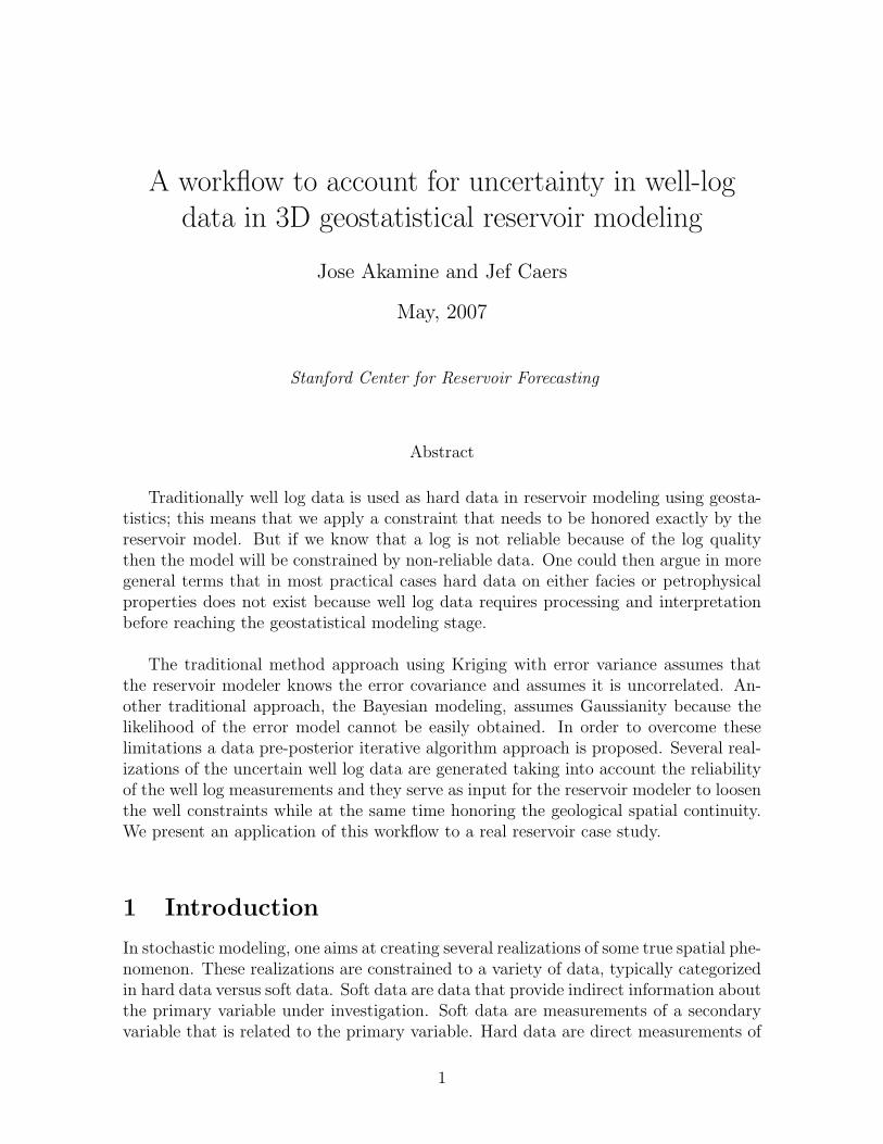
Traditionally well log data is used as hard data in reservoir modeling using geosta-tistics; this means that we apply a constraint that needs to be honored exactly by thereservoir model. But if we know that a log is not reliable because of the log qualitythen the model will be constrained by non-reliable data. One could then argue in moregeneral terms that in most practical cases hard data on either facies or petrophysicalproperties does not exist because well log data requires processing and interpretationbefore reaching the geostatistical modeling stage.
The traditional method approach using Kriging with error variance assumes thatthe reservoir modeler knows the error covariance and assumes it is uncorrelated. An-other traditional approach, the Bayesian modeling, assumes Gaussianity because thelikelihood of the error model cannot be easily obtained. In order to overcome theselimitations a data pre-posterior iterative algorithm approach is proposed. Several real-izations of the uncertain well log data are generated taking into account the reliabilityof the well log measurements and they serve as input for the reservoir modeler to loosenthe well constraints while at the same time honoring the geological spatial continuity.We present an application of this workflow to a real reservoir case study.
1 Introduction
In stochastic modeling, one aims at creating several realizations of some true spatial phe-nomenon. These realizations are constrained to a variety of data, typically categorizedin hard data versus soft data. Soft data are data that provide indirect information aboutthe primary variable under investigation. Soft data are measurements of a secondaryvariable that is related to the primary variable. Hard data are direct measurements of
1
A workflow to account for uncertainty in well-log data in 3D geostatistical reservoirmodeling
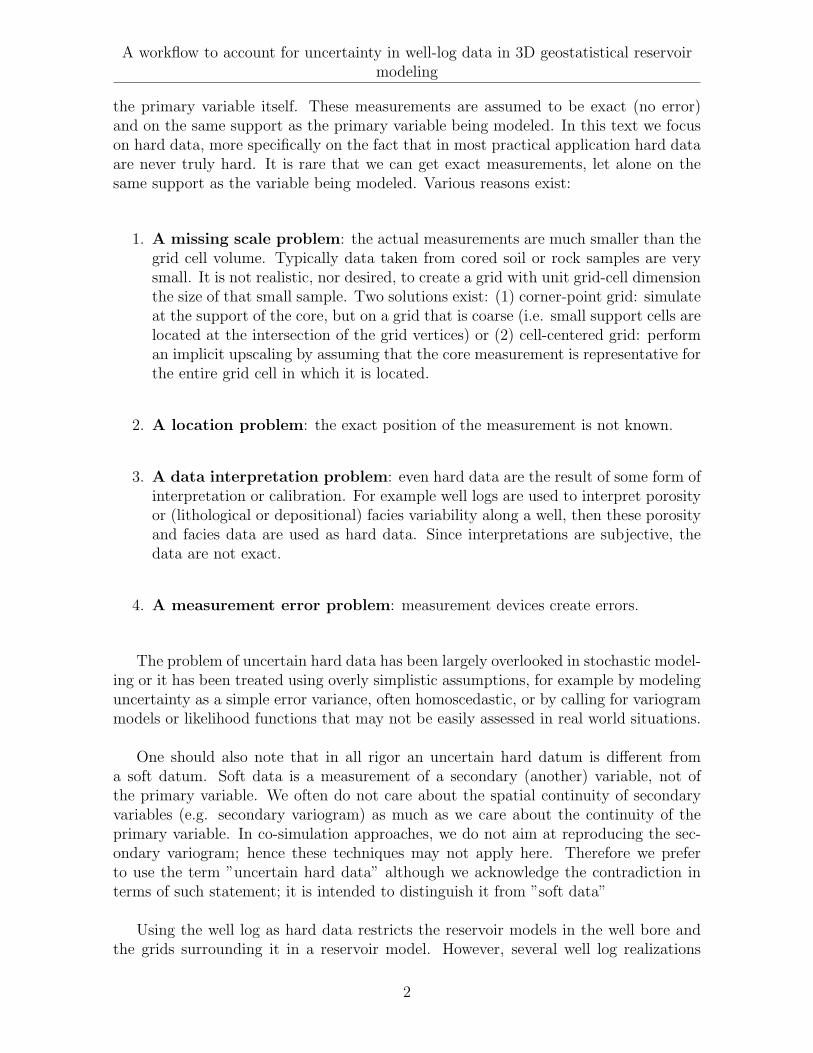
the primary variable itself. These measurements are assumed to be exact (no error)and on the same support as the primary variable being modeled. In this text we focuson hard data, more specifically on the fact that in most practical application hard dataare never truly hard. It is rare that we can get exact measurements, let alone on thesame support as the variable being modeled. Various reasons exist:
1. A missing scale problem: the actual measurements are much smaller than thegrid cell volume. Typically data taken from cored soil or rock samples are verysmall. It is not realistic, nor desired, to create a grid with unit grid-cell dimensionthe size of that small sample. Two solutions exist: (1) corner-point grid: simulateat the support of the core, but on a grid that is coarse (i.e. small support cells arelocated at the intersection of the grid vertices) or (2) cell-centered grid: performan implicit upscaling by assuming that the core measurement is representative forthe entire grid cell in which it is located.
2. A location problem: the exact position of the measurement is not known.
3. A data interpretation problem: even hard data are the result of some form ofinterpretation or calibration. For example well logs are used to interpret porosityor (lithological or depositional) facies variability along a well, then these porosityand facies data are used as hard data. Since interpretations are subjective, thedata are not exact.
4. A measurement error problem: measurement devices create errors.
The problem of uncertain hard data has been largely overlooked in stochastic model-ing or it has been treated using overly simplistic assumptions, for example by modelinguncertainty as a simple error variance, often homoscedastic, or by calling for variogrammodels or likelihood functions that may not be easily assessed in real world situations.
One should also note that in all rigor an uncertain hard datum is different froma soft datum. Soft data is a measurement of a secondary (another) variable, not ofthe primary variable. We often do not care about the spatial continuity of secondaryvariables (e.g. secondary variogram) as much as we care about the continuity of theprimary variable. In co-simulation approaches, we do not aim at reproducing the sec-ondary variogram; hence these techniques may not apply here. Therefore we preferto use the term ”uncertain hard data” although we acknowledge the contradiction interms of such statement; it is intended to distinguish it from ”soft data”
Using the well log as hard data restricts the reservoir models in the well bore andthe grids surrounding it in a reservoir model. However, several well log realizations
2
A workflow to account for uncertainty in well-log data in 3D geostatistical reservoirmodeling
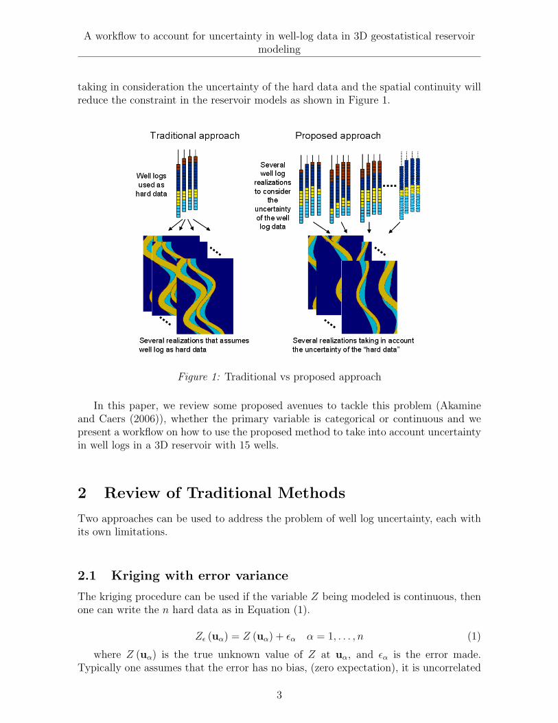
taking in consideration the uncertainty of the hard data and the spatial continuity willreduce the constraint in the reservoir models as shown in Figure 1.
Figure 1: Traditional vs proposed approach
In this paper, we review some proposed avenues to tackle this problem (Akamineand Caers (2006)), whether the primary variable is categorical or continuous and wepresent a workflow on how to use the proposed method to take into account uncertaintyin well logs in a 3D reservoir with 15 wells.
2 Review of Traditional Methods
Two approaches can be used to address the problem of well log uncertainty, each withits own limitations.
2.1 Kriging with error variance
The kriging procedure can be used if the variable Z being modeled is continuous, thenone can write the n hard data as in Equation (1).
Zε (uα) = Z (uα) + εα α = 1, . . . , n (1)
where Z (uα) is the true unknown value of Z at uα, and εα is the error made.Typically one assumes that the error has no bias, (zero expectation), it is uncorrelated
3
A workflow to account for uncertainty in well-log data in 3D geostatistical reservoirmodeling
with Z, but errors may be correlated with each other, i.e. some variance/covariancemodel of the error exists as in Equation (2).
E [εαεβ] = ercovαβ α, β = 1, . . . , n (2)
The simple kriging estimator (zero mean case) is shown in Equation (3),
Z∗ (u) =n∑
α=1
λα (Z (u)) + εα (3)
and the kriging system is shown in Equation (4).
n∑β=1
λβ (C (uβ − uα) + ercovαβ) = C (u− uα) (4)
This kriging procedure can be implemented in sgsim (multi-Gaussian Assumption)or dssim (no-Multi-Gaussian assumption), however dssim does not require a Gaussiantranform to change the variance of Z to unity neither assume that the variance of theerror has the same transform.
The limitation of this approach is that we assume that we know the error covarianceercovαβ and it will work only for continuous variables.
2.2 Bayesian modeling
In a Bayesian framework, the joint uncertainty of all variables Z (u), denoted as Z, ismodeled using the posterior probability as in Equation (5).
f (Z| {Zε (uα) , α = 1, . . . , n}) ≈ f (Zε (uα) , α = 1, . . . , n|Z) f (Z) (5)
If the errors are assumed independent of the signal and of each other, then condi-tional independence applies and the posterior probability will be as in Equation (6).
f (Z| {Zε (uα) , α = 1, . . . , n}) ≈ f (Z)n∏
α=1
f (Zε (uα) |Z) (6)
And if no bias in the error is present, then:
f (Zε (uα) |Z) = f (ε) (7)
In other words, the likelihood distribution is reduced to an error model. In a multi-Gaussian context, one assumes that all f are Gaussian, whether conditional, univariateor multi-variate. For the error model a Gaussian distribution with zero mean and errorvariance is used.
Theoretically, in all generality, the Bayesian framework in Equation (7) does notrequire assumptions of multi-Gaussianity or conditional independence. However, in
4
A workflow to account for uncertainty in well-log data in 3D geostatistical reservoirmodeling
practice, this assumptions are often needed to make the methods practical, first froma sampling point of view, secondly because the data is not available to fully determinethe likelihood distribution on Equation (7). The likelihood distribution expresses thejoint uncertainty about the data for any possible reference field z. This would requireone to know the exact forward model g that represents the link between the referencefield and the data emanating from taking measurements from it as in Equation (8).
{Zε (uα) , α = 1, . . . , n} = g (Z) (8)
In the case of errors of measurement devices, this may not be well-known. Forexample, we cannot possibly model the complete physics of a neutron-logging tool topredict what its response would be under certain field conditions. Moreover, in the casethe error is due to interpretation it is not clear at all what the forward model is, theng is function of the (human) interpreter.
A second limitation lies in the fact that these method also applies to continuos vari-ables.
3 The Data Set
The confidential well log data used in Section 4, Proposed Method , is introduced. The15 wells belongs to a distal supra fan environment in a sub-marine delta depositionalsystem. The oldest well was logged in 1976 and the newest was logged in 2004. Thetechnology used ranges from a wireline ”triple-combo” to logging while drilling tech-nology (LWD).
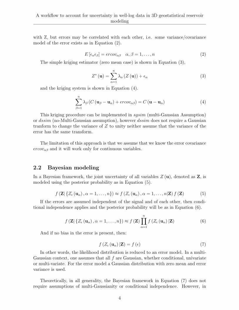
The reservoir has 100 × 100 × 50 cells. The cell size is 120m × 100m × 2ft. In thereservoir portion of interest the 15 wells are mostly vertical. Figure 2 shows the welldistribution in the Stanford Geostatistical Modeling Software (SGeMS).
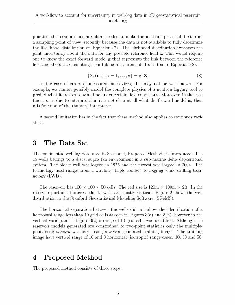
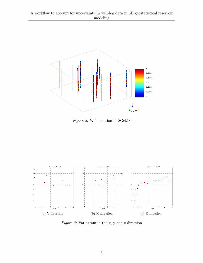
The horizontal separation between the wells did not allow the identification of ahorizontal range less than 10 grid cells as seen in Figures 3(a) and 3(b), however in thevertical variogram in Figure 3(c) a range of 10 grid cells was identified. Although thereservoir models generated are constrained to two-point statistics only the multiple-point code snesim was used using a sisim generated training image. The trainingimage have vertical range of 10 and 3 horizontal (isotropic) range-cases: 10, 30 and 50.
4 Proposed Method
The proposed method consists of three steps:
5
A workflow to account for uncertainty in well-log data in 3D geostatistical reservoirmodeling
Figure 2: Well location in SGeMS
(a) Y-direction (b) X-direction (c) Z-direction
Figure 3: Variogram in the x, y and z direction
6
A workflow to account for uncertainty in well-log data in 3D geostatistical reservoirmodeling
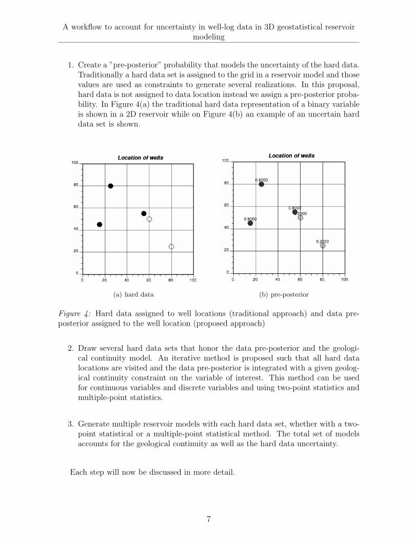
1. Create a ”pre-posterior” probability that models the uncertainty of the hard data.Traditionally a hard data set is assigned to the grid in a reservoir model and thosevalues are used as constraints to generate several realizations. In this proposal,hard data is not assigned to data location instead we assign a pre-posterior proba-bility. In Figure 4(a) the traditional hard data representation of a binary variableis shown in a 2D reservoir while on Figure 4(b) an example of an uncertain harddata set is shown.
(a) hard data (b) pre-posterior
Figure 4: Hard data assigned to well locations (traditional approach) and data pre-posterior assigned to the well location (proposed approach)
2. Draw several hard data sets that honor the data pre-posterior and the geologi-cal continuity model. An iterative method is proposed such that all hard datalocations are visited and the data pre-posterior is integrated with a given geolog-ical continuity constraint on the variable of interest. This method can be usedfor continuous variables and discrete variables and using two-point statistics andmultiple-point statistics.
3. Generate multiple reservoir models with each hard data set, whether with a two-point statistical or a multiple-point statistical method. The total set of modelsaccounts for the geological continuity as well as the hard data uncertainty.
Each step will now be discussed in more detail.
7
A workflow to account for uncertainty in well-log data in 3D geostatistical reservoirmodeling
5 The data pre-posterior
In most cases, one does not have access to likelihood distributions; instead it is morepractical to assume that for each hard data location, one can provide a probability dis-tribution describing the possible outcomes of hard data at that location as in Equation(9).
f (Zε (uα) |measurement at uα) (9)
In other words, given the results from a measurement device, one has either in-terpreted or calibrated the possible range of values and their frequencies. Note thatEquation (9) does not require a forward model, it can be directly obtained from themeasurements. We call Equation (9) a data pre-posterior, i.e. some prior informationon the true value at u is available, however it is not yet a posterior distribution as otherdata sources are not yet accounted for (e.g. spatial continuity, other hard data, softdata, etc . . . ). We argue that working with data pre-posteriors is more practical thanworking with data likelihoods. Indeed, a data-pre-posterior could be obtained for thetype of errors described in the introduction:
1. Missing scale: a fine-scale with unit-grid cell simulation of the spatial variablebased on geological or other information could be done. Using many simulations,one could calculate Equation (9) empirically, i.e. tabulate frequency distributionof the entire grid-block property is for a given small-scale measurement.
2. Location: this problem could be handled similar as in the missing scale problem.
3. Interpretation: the interpreter could provide, based on his expertise, a distri-bution of values rather than a single interpretation. This distribution could bebased on a confidence interval that he/she places on that single interpretation.
4. Measurement error: a simple Gaussian model with error variance could beused, or any other probability distribution for that matter.
Note that the data pre-posterior concept also applies to discrete variables, whereinstead of a hard indicator datum, a probability can be provided expressing the uncer-tainty of the indicator event occurring:
Pr (I (uα) = 1|measurement at uα) (10)
Following we present one workflow to obtain the data pre-posterior.
8
A workflow to account for uncertainty in well-log data in 3D geostatistical reservoirmodeling
5.1 A workflow to obtain the data pre-posterior
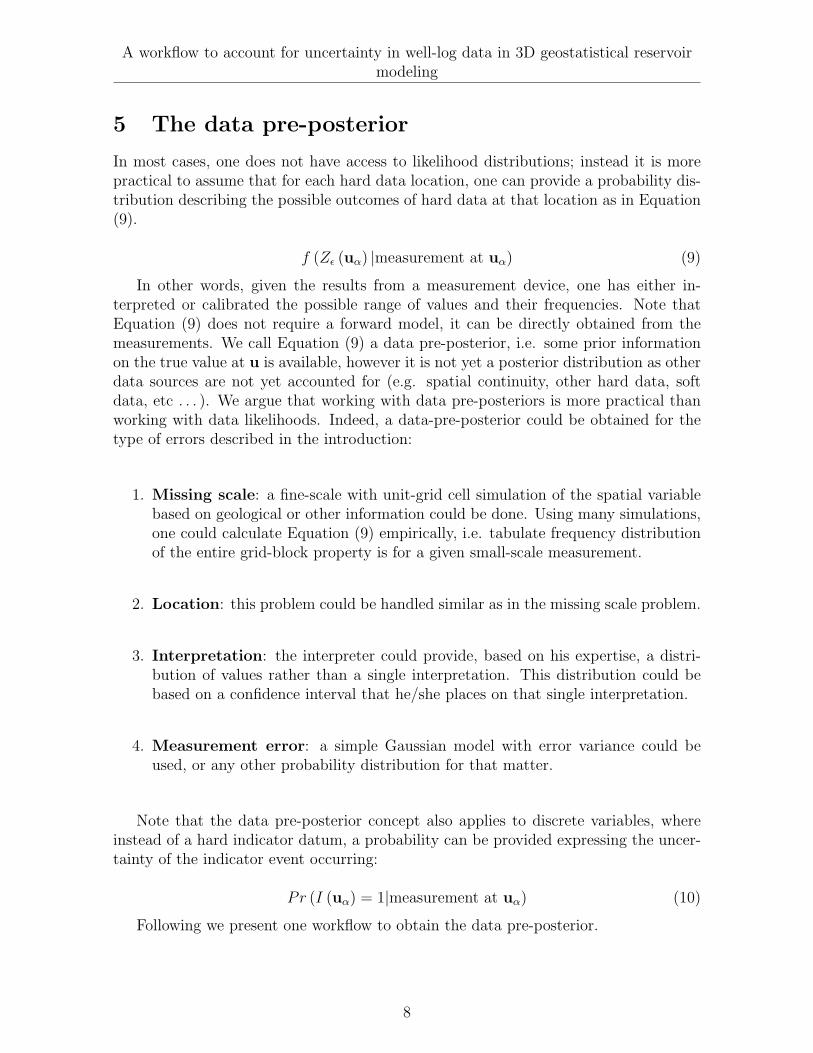
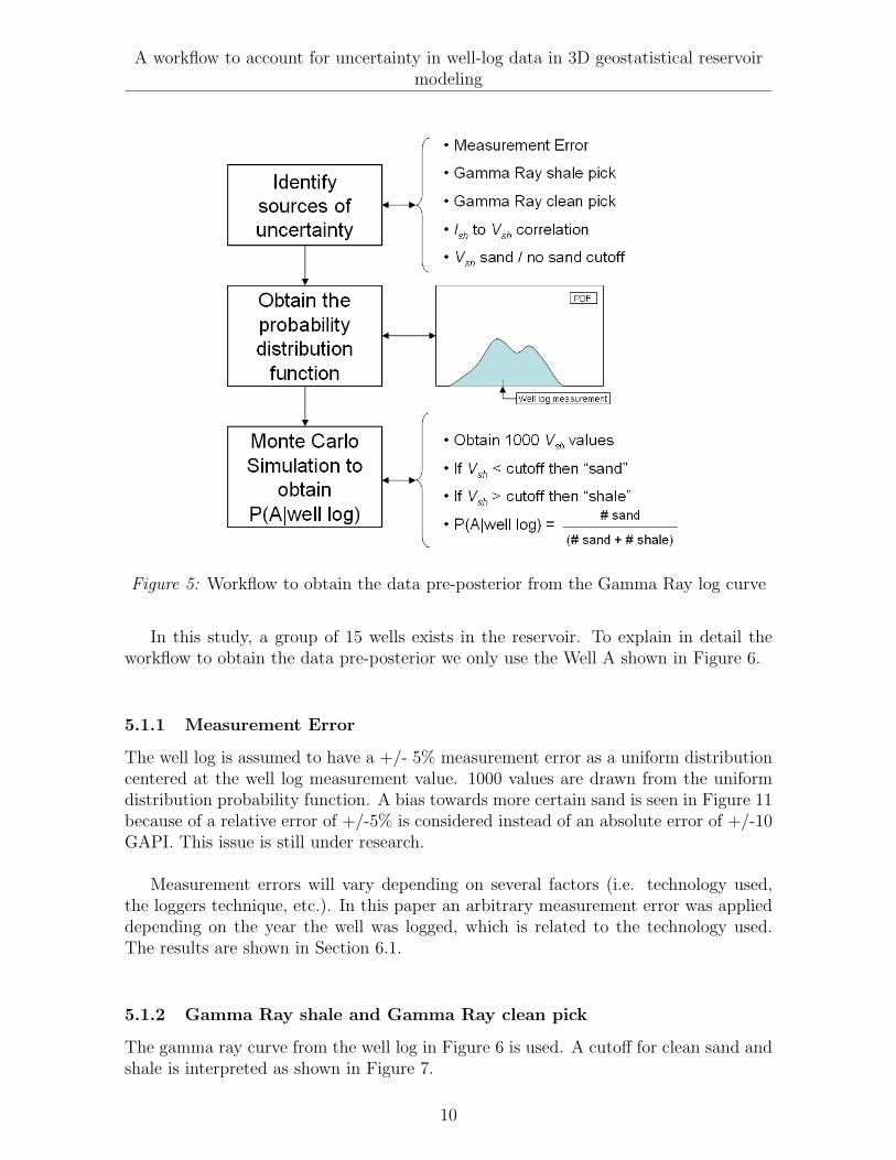
The workflow used to obtain the data pre-posterior from 15 wells using the Gamma Raylog curve is shown in Figure 5. The data pre-posterior for discrete variables in Equation(10) is equivalent in this case to the probability of having sand given the Gamma Raylog: P (A|well log) where A is sand and the well log is the Gamma Ray log curve.
The P (A|well log) is obtained by a direct relationship to the shale volume content(Vsh).
In the case of the Gamma Ray log the shale volume content (Vsh) can be linearlyrelated to the shale index (Ish) as in Equation (11),
Vsh = Ish =γlog − γclean
γshale − γclean
(11)
where γlog is the gamma ray response in the zone of interest obtained from the log,γclean is the average gamma ray response in the cleanest formations and γshale is theaverage gamma ray response in shales. The γclean and γshale are values that need tobe chosen by the interpreter, therefore it can be considered as an additional source ofuncertainty.
Alternative non-linear correlations between Vsh and Ish exists as explained in thefollowing sub-sections. The existence of these alternatives is an additional source ofscenario-based uncertainty.
In the workflow, first we identify the sources of uncertainty that affects the GammaRay log. The 4 sources of uncertainties analyzed are:
1. Measurement Error
2. Gamma Ray shale pick
3. Gamma Ray clean pick
4. Ish to Vsh Correlation curve selection
5. Vsh sand / no sand cutoff
Secondly, we construct a probability distribution function (pdf) that integrates thesesources of uncertainties into a single model.
Third, using Monte Carlo simulation we draw from the pdf and compare it to a Vsh
cutoff that differentiates sand from no-sand. The fraction of values that are drawn assand will form the data preposterior: P (A|well log).
Each step will be explained in more detailed in the following sub-sections.
9
A workflow to account for uncertainty in well-log data in 3D geostatistical reservoirmodeling
Figure 5: Workflow to obtain the data pre-posterior from the Gamma Ray log curve
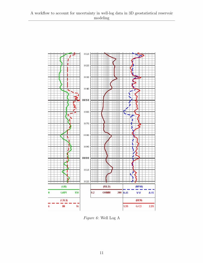
In this study, a group of 15 wells exists in the reservoir. To explain in detail theworkflow to obtain the data pre-posterior we only use the Well A shown in Figure 6.
5.1.1 Measurement Error
The well log is assumed to have a +/- 5% measurement error as a uniform distributioncentered at the well log measurement value. 1000 values are drawn from the uniformdistribution probability function. A bias towards more certain sand is seen in Figure 11because of a relative error of +/-5% is considered instead of an absolute error of +/-10GAPI. This issue is still under research.
Measurement errors will vary depending on several factors (i.e. technology used,the loggers technique, etc.). In this paper an arbitrary measurement error was applieddepending on the year the well was logged, which is related to the technology used.The results are shown in Section 6.1.
5.1.2 Gamma Ray shale and Gamma Ray clean pick
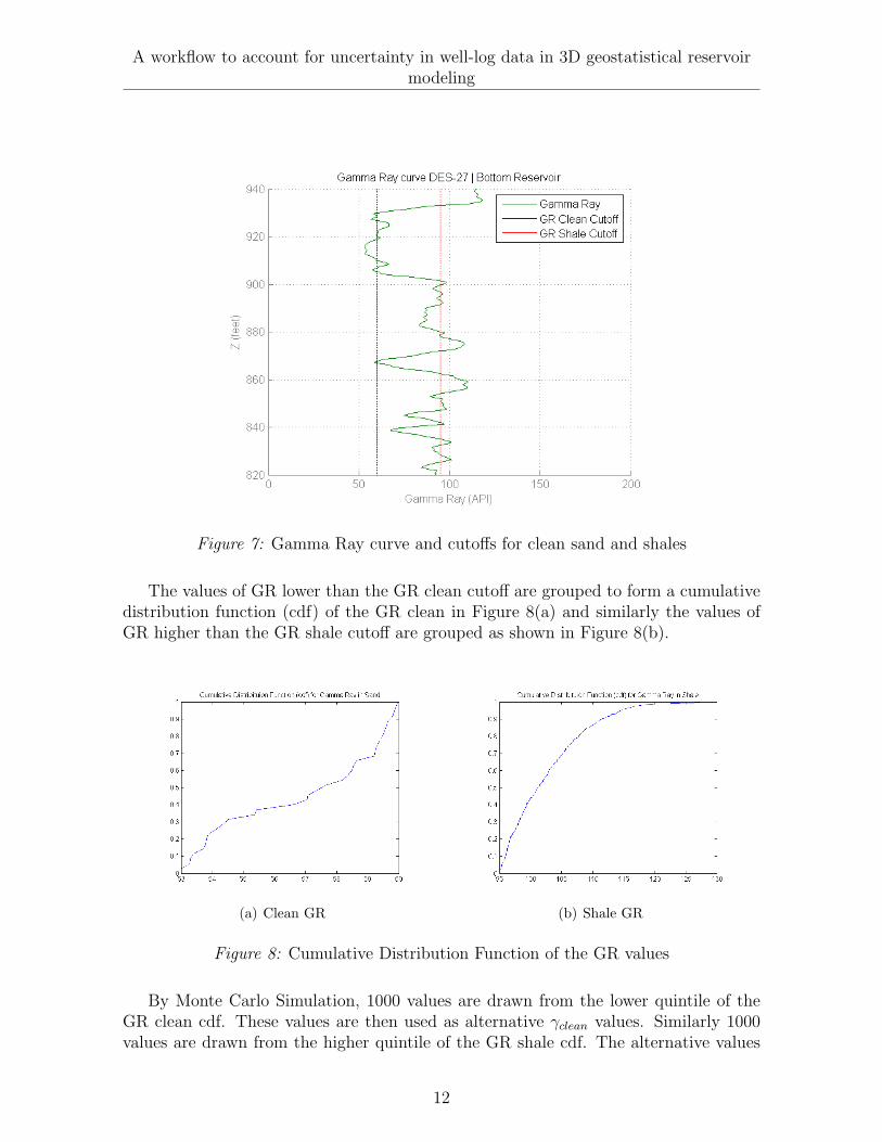
The gamma ray curve from the well log in Figure 6 is used. A cutoff for clean sand andshale is interpreted as shown in Figure 7.
10
A workflow to account for uncertainty in well-log data in 3D geostatistical reservoirmodeling
Figure 6: Well Log A
11
A workflow to account for uncertainty in well-log data in 3D geostatistical reservoirmodeling
Figure 7: Gamma Ray curve and cutoffs for clean sand and shales
The values of GR lower than the GR clean cutoff are grouped to form a cumulativedistribution function (cdf) of the GR clean in Figure 8(a) and similarly the values ofGR higher than the GR shale cutoff are grouped as shown in Figure 8(b).
(a) Clean GR (b) Shale GR
Figure 8: Cumulative Distribution Function of the GR values
By Monte Carlo Simulation, 1000 values are drawn from the lower quintile of theGR clean cdf. These values are then used as alternative γclean values. Similarly 1000values are drawn from the higher quintile of the GR shale cdf. The alternative values
12
A workflow to account for uncertainty in well-log data in 3D geostatistical reservoirmodeling
are used as the γclean and γshale respectively in Equation (11).
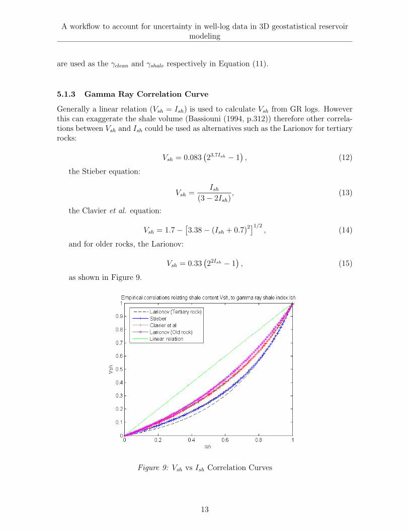
5.1.3 Gamma Ray Correlation Curve
Generally a linear relation (Vsh = Ish) is used to calculate Vsh from GR logs. Howeverthis can exaggerate the shale volume (Bassiouni (1994, p.312)) therefore other correla-tions between Vsh and Ish could be used as alternatives such as the Larionov for tertiaryrocks:
Vsh = 0.083(23.7Ish − 1
), (12)
the Stieber equation:
Vsh =Ish
(3− 2Ish), (13)
the Clavier et al. equation:
Vsh = 1.7−[3.38− (Ish + 0.7)2]1/2
, (14)
and for older rocks, the Larionov:
Vsh = 0.33(22Ish − 1
), (15)
as shown in Figure 9.
Figure 9: Vsh vs Ish Correlation Curves
13
A workflow to account for uncertainty in well-log data in 3D geostatistical reservoirmodeling
In addition to these correlations one can develop correlations specifically for a for-mation or geological unit of interest.
We assign a probability of 60% for the linear interpretation to be an appropiatemodel; all other interpretations are assigned a 10% probability.
5.1.4 Vsh sand / shale cutoff
To differentiate between sand and shale a Vsh cutoff is selected. In this workflow theVsh cutoff is considered also a source of uncertainty since it is also selected by the in-terpreter, therefore by Monte Carlo simulation 1000 values from a uniform probabilitydistribution function between 0.4 and 0.6 are used as the Vsh cutoff.
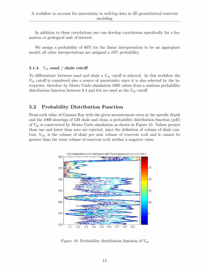
5.2 Probability Distribution Function
From each value of Gamma Ray with the given measurement error at the specific depthand the 1000 drawings of GR shale and clean, a probability distribution function (pdf)of Vsh is constructed by Monte Carlo simulation as shown in Figure 10. Values greaterthan one and lower than zero are rejected, since the definition of volume of shale con-tent, Vsh, is the volume of shale per unit volume of reservoir rock and it cannot begreater than the total volume of reservoir rock neither a negative value.
Figure 10: Probability distribution function of Vsh
14
A workflow to account for uncertainty in well-log data in 3D geostatistical reservoirmodeling
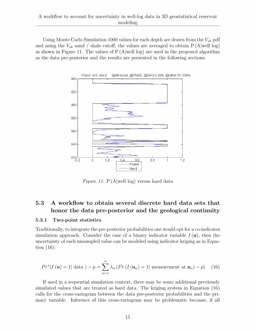
Using Monte Carlo Simulation 1000 values for each depth are drawn from the Vsh pdfand using the Vsh sand / shale cutoff, the values are averaged to obtain P (A|well log)as shown in Figure 11. The values of P (A|well log) are used in the proposed algorithmas the data pre-posterior and the results are presented in the following sections.
Figure 11: P (A|well log) versus hard data
5.3 A workflow to obtain several discrete hard data sets thathonor the data pre-posterior and the geological continuity
5.3.1 Two-point statistics
Traditionally, to integrate the pre-posterior probabilities one would opt for a co-indicatorsimulation approach. Consider the case of a binary indicator variable I (u), then theuncertainty of each unsampled value can be modeled using indicator kriging as in Equa-tion (16):
Pr∗(I (u) = 1| data )− p =n∑
α=1
λα (Pr (I (uα) = 1| measurement at uα)− p) (16)
If used in a sequential simulation context, there may be some additional previouslysimulated values that are treated as hard data. The kriging system in Equation (16)calls for the cross-variogram between the data pre-posterior probabilities and the pri-mary variable. Inference of this cross-variogram may be problematic because, if all
15
A workflow to account for uncertainty in well-log data in 3D geostatistical reservoirmodeling
hard data are uncertain, no direct observation of the primary variable is available, af-ter all that is the premise here! A possible solution would be to create ”pseudo harddata” by means of classification from the data pre-posterior, then infer primary andcross-variogram. However, such classification is done independently from one locationto another, ignoring spatial continuity, moreover, since the hard data are obtained fromthe data pre-posterior, one may overestimate the dependency between the pre-posteriorprobabilities and primary variable.
If a cross-variogram cannot be inferred, than this essentially means that the redun-dancy between the primary variable (in essence its spatial continuity) and the uncer-tain hard data cannot be accurately assessed. However, recall that the goal of spatialsimulation is not primarily to assess data redundancy (i.e. model variogram and cross-variogram), but to create realizations that reflect some prior spatial continuity modeland fit the data either exactly (hard) or to some extent (uncertain hard). Hence, wereverse the problem: assume we know the redundancy, then, for that given redundancy,does the resulting realization reflect the important properties we want to impose onthem? In other words, we could by trail and error try various variogram models untilwe find one that does the job. However, since variogram models are tedious to handle(multiple parameters) and since the information given here is in terms of probabilities,a better alternative would be to frame the redundancy issue directly in terms of prob-abilities rather than work with variograms.
Journel (2002) proposes a model (in terms of probabilities) that allows to decom-pose the problem of assessing the uncertainty about some unknown from different datasources, into a problem of assessing the information content of each data source onthe unknown separately from assessing the redundancy of information between datasources. If D1, D2,. . . , Dn data sources are available about some unknown A, then theposterior probability P (A|D1, D2, . . . , Dn) can be assessed as in Equation (17):
P (A|D1, D2, . . . , Dn) =1
1 + x∈ [0, 1] (17)
where:
x
x0
=n∏
i=1
(xi
x0
)τi
(18)
and the data probability ratios x0, x1, . . . , xn and the target ratio x, all valued in[0,∞] as:
x0 =1− P (A)
P (A), x1 =
1− P (A|D1)
P (A|D1), . . . , xn =
1− P (A|Dn)
P (A|Dn)and x =
1− P (A|D1, . . . , Dn)
P (A|D1, . . . , Dn)(19)
Each P (A|Di) quantifies the information content of data source Di on the unknownA. The τi values model the redundancy between data source Di and all other data
16
A workflow to account for uncertainty in well-log data in 3D geostatistical reservoirmodeling
sources taken jointly.
Consider now a two-step approach to conditioning realizations to the data pre-posteriors. In the first step, we propose to generate multiple hard data sets, by asequential iterative sampling (Gibbs sampling) from the data pre-posterior. This sam-pling method, explained in full detail next, accounts for both the data pre-posterioras well as the spatial continuity of the primary variable (supposedly available). In thesecond step, one generates multiple realizations from these multiple hard datasets usingthe standard sequential simulation procedure.
To generate one single hard data set from the data pre-posterior, we use the follow-ing algorithm:
1. Define an order to visit the hard data locations
2. Draw an initial i(o) (uα) , α = 1, . . . , n from the data pre-posterior
3. Start to iterate k = 1, . . . , K
(a) Loop over all hard data locations α = 1, . . . , n
i. Determine by indicator kriging Pr(I(k) (uα) = 1| all i(k−1) (uβ) , β 6= α
)ii. Use the tau model to combine Pr
(I(k) (uα) = 1| all i(k−1) (uβ) , β 6= α
)and Pr (I (uα) = 1| measurement at uα) into a single posterior model.
iii. Draw a sample value i(k) (uα) from this posterior model
One may argue that an approach using indicator kriging with soft data usingMarkov-Bayes model can be used to integrate soft information into a posterior prob-ability value. However such procedure only retains the closest soft data (which is atthe same location), hence it does not use soft data from other locations. The uncertainhard data, Pr (I (uα) = 1| measurement at uα), at other locations should be taken intoaccount when modeling the local ccdf to ensure the correct spatial continuity.
If one would not iterate then the first hard data value would simply be a samplefrom the data pre-posterior, it would not take into account the ”uncertain hard data”at any other locations. Hence, after the first iteration, the spatial continuity model maynot be honored, since only the last simulated value depends on the previously simulateddatum. This is not a problem in traditional sequential simulation, since for the firstvalue to be simulated one either has no hard data (unconditional) or some (certain)hard data that are accounted for in the kriging.
This procedure is similar to a Gibbs sampler in Markov chain Monte Carlo simula-tion, but the goal is quite different from Gibbs sampling. In traditional Gibbs samplingthe idea is to sample from a given joint posterior distribution by sequentially and iter-atively sampling from conditional distributions derived from that posterior. However,
17
A workflow to account for uncertainty in well-log data in 3D geostatistical reservoirmodeling
the posterior here is unknown; in fact, one should view the above procedure as a wayto generate an algorithmic-based posterior, in other words, the algorithm determinesthe ultimate posterior sampled, not the other way around.
The tau values are important since they will determine whether the primary vari-ogram is reproduced or not. Hence, some trial and error would be required to find asuitable range for the tau values.
While the iterative procedure is slower than a sequential one, one only has to iterateover the data locations, moreover, the kriging needs to be done only once, hence thisprocess will be very fast.
5.3.2 Multiple-point statistics
The procedure would essentially remain the same except that one uses a training imageand search tree to determine the conditional probability in Equation (20):
Pr(I(k) (uα) = 1| all i(k−1) (uβ) , β 6= α
)(20)
The algorithm model proposes to generate multiple hard data sets and use themas an input in the snesim algorithm (Strebelle (2002)). Instead of having a uniquedeterministic data set, the model simulates several realizations of the well logs.
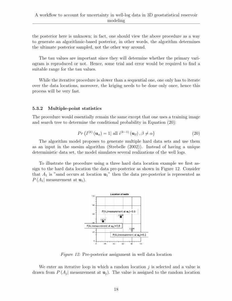
To illustrate the procedure using a three hard data location example we first as-sign to the hard data location the data pre-posterior as shown in Figure 12. Considerthat A1 is ”sand occurs at location u1” then the data pre-posterior is represented asP (A1| measurement at u1).
Figure 12: Pre-posterior assignment in well data location
We enter an iterative loop in which a random location j is selected and a value isdrawn from P (Aj| measurement at uj). The value is assigned to the random location
18
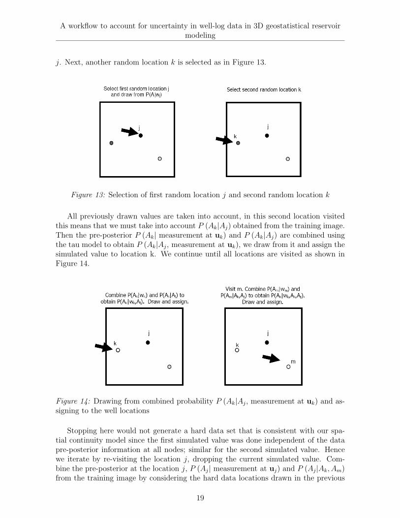
A workflow to account for uncertainty in well-log data in 3D geostatistical reservoirmodeling
j. Next, another random location k is selected as in Figure 13.
Figure 13: Selection of first random location j and second random location k
All previously drawn values are taken into account, in this second location visitedthis means that we must take into account P (Ak|Aj) obtained from the training image.Then the pre-posterior P (Ak| measurement at uk) and P (Ak|Aj) are combined usingthe tau model to obtain P (Ak|Aj, measurement at uk), we draw from it and assign thesimulated value to location k. We continue until all locations are visited as shown inFigure 14.
Figure 14: Drawing from combined probability P (Ak|Aj, measurement at uk) and as-signing to the well locations
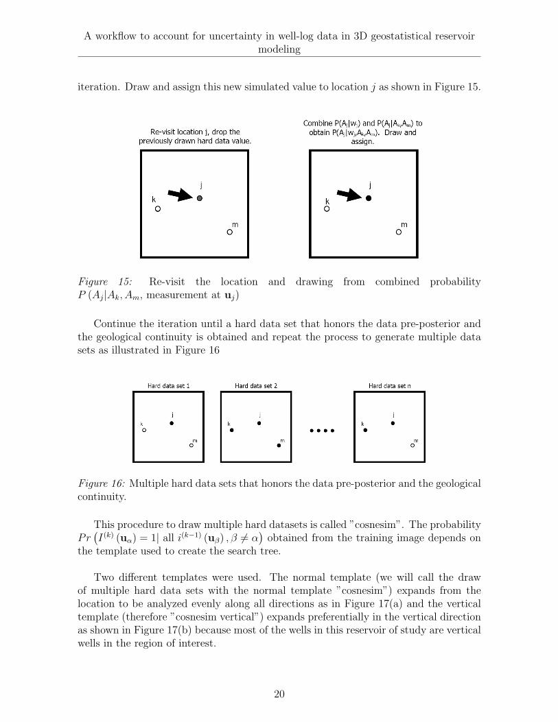
Stopping here would not generate a hard data set that is consistent with our spa-tial continuity model since the first simulated value was done independent of the datapre-posterior information at all nodes; similar for the second simulated value. Hencewe iterate by re-visiting the location j, dropping the current simulated value. Com-bine the pre-posterior at the location j, P (Aj| measurement at uj) and P (Aj|Ak, Am)from the training image by considering the hard data locations drawn in the previous
19
A workflow to account for uncertainty in well-log data in 3D geostatistical reservoirmodeling
iteration. Draw and assign this new simulated value to location j as shown in Figure 15.
Figure 15: Re-visit the location and drawing from combined probabilityP (Aj|Ak, Am, measurement at uj)
Continue the iteration until a hard data set that honors the data pre-posterior andthe geological continuity is obtained and repeat the process to generate multiple datasets as illustrated in Figure 16
Figure 16: Multiple hard data sets that honors the data pre-posterior and the geologicalcontinuity.
This procedure to draw multiple hard datasets is called ”cosnesim”. The probabilityPr
(I(k) (uα) = 1| all i(k−1) (uβ) , β 6= α
)obtained from the training image depends on
the template used to create the search tree.
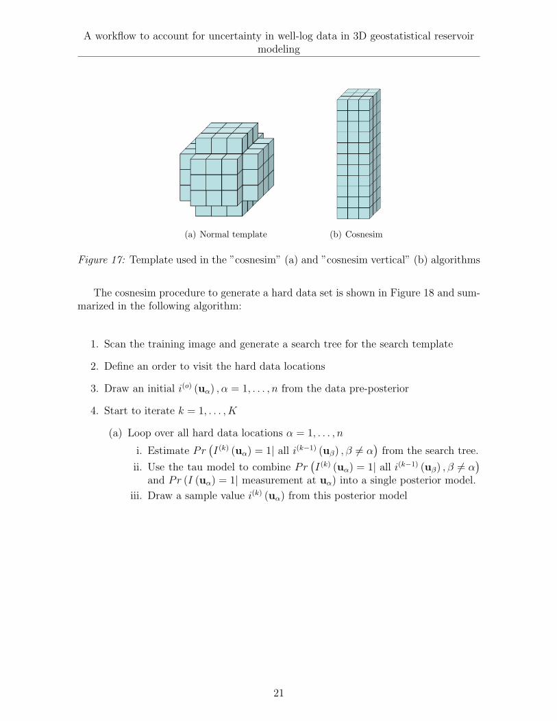
Two different templates were used. The normal template (we will call the drawof multiple hard data sets with the normal template ”cosnesim”) expands from thelocation to be analyzed evenly along all directions as in Figure 17(a) and the verticaltemplate (therefore ”cosnesim vertical”) expands preferentially in the vertical directionas shown in Figure 17(b) because most of the wells in this reservoir of study are verticalwells in the region of interest.
20
A workflow to account for uncertainty in well-log data in 3D geostatistical reservoirmodeling
(a) Normal template (b) Cosnesim
Figure 17: Template used in the ”cosnesim” (a) and ”cosnesim vertical” (b) algorithms
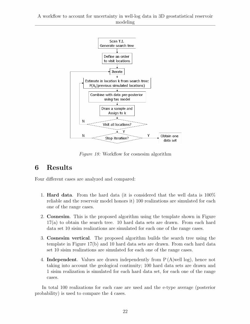
The cosnesim procedure to generate a hard data set is shown in Figure 18 and sum-marized in the following algorithm:
1. Scan the training image and generate a search tree for the search template
2. Define an order to visit the hard data locations
3. Draw an initial i(o) (uα) , α = 1, . . . , n from the data pre-posterior
4. Start to iterate k = 1, . . . , K
(a) Loop over all hard data locations α = 1, . . . , n
i. Estimate Pr(I(k) (uα) = 1| all i(k−1) (uβ) , β 6= α
)from the search tree.
ii. Use the tau model to combine Pr(I(k) (uα) = 1| all i(k−1) (uβ) , β 6= α
)and Pr (I (uα) = 1| measurement at uα) into a single posterior model.
iii. Draw a sample value i(k) (uα) from this posterior model
21
A workflow to account for uncertainty in well-log data in 3D geostatistical reservoirmodeling
Figure 18: Workflow for cosnesim algorithm
6 Results
Four different cases are analyzed and compared:
1. Hard data. From the hard data (it is considered that the well data is 100%reliable and the reservoir model honors it) 100 realizations are simulated for eachone of the range cases.
2. Cosnesim. This is the proposed algorithm using the template shown in Figure17(a) to obtain the search tree. 10 hard data sets are drawn. From each harddata set 10 sisim realizations are simulated for each one of the range cases.
3. Cosnesim vertical. The proposed algorithm builds the search tree using thetemplate in Figure 17(b) and 10 hard data sets are drawn. From each hard dataset 10 sisim realizations are simulated for each one of the range cases.
4. Independent. Values are drawn independently from P (A|well log), hence nottaking into account the geological continuity; 100 hard data sets are drawn and1 sisim realization is simulated for each hard data set, for each one of the rangecases.
In total 100 realizations for each case are used and the e-type average (posteriorprobability) is used to compare the 4 cases.
22
A workflow to account for uncertainty in well-log data in 3D geostatistical reservoirmodeling
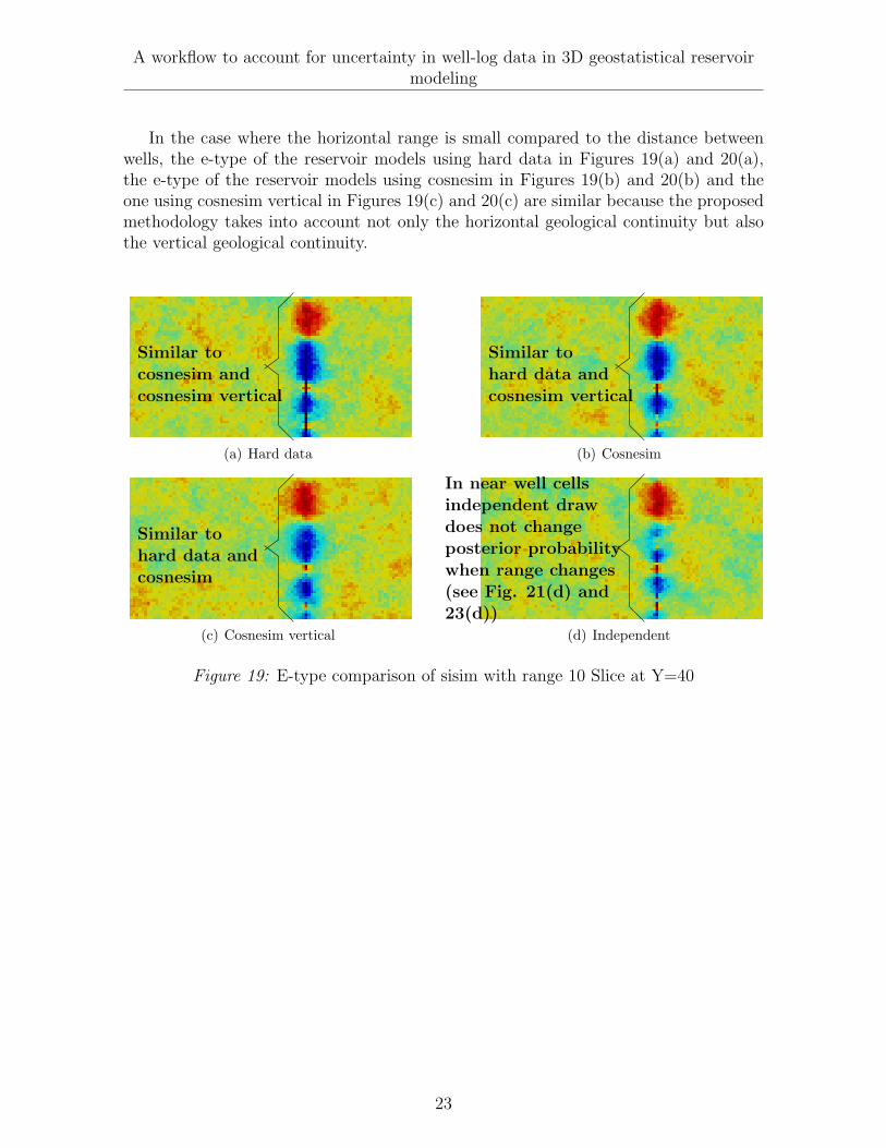
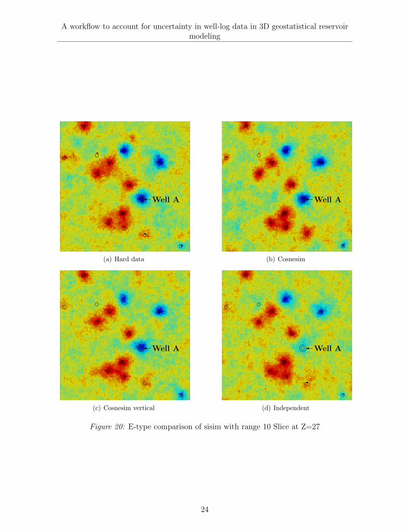
In the case where the horizontal range is small compared to the distance betweenwells, the e-type of the reservoir models using hard data in Figures 19(a) and 20(a),the e-type of the reservoir models using cosnesim in Figures 19(b) and 20(b) and theone using cosnesim vertical in Figures 19(c) and 20(c) are similar because the proposedmethodology takes into account not only the horizontal geological continuity but alsothe vertical geological continuity.
(a) Hard data (b) Cosnesim
�
�Z
@
�
�Z
@
Similar tocosnesim andcosnesim vertical
Similar tohard data andcosnesim vertical
(c) Cosnesim vertical (d) Independent
�
�Z
@
Similar tohard data andcosnesim
�
�Z
@
In near well cellsindependent drawdoes not changeposterior probabilitywhen range changes(see Fig. 21(d) and23(d))
Figure 19: E-type comparison of sisim with range 10 Slice at Y=40
23
A workflow to account for uncertainty in well-log data in 3D geostatistical reservoirmodeling
(a) Hard data (b) Cosnesim
dd
di� Well A
d dd
ddd
dd d
d
d
dd
ddi� Well A
d dd
ddd
dd d
d
d
d
(c) Cosnesim vertical (d) Independent
dd
di� Well A
d dd
ddd
dd d
d
d
dd
ddi� Well A
d dd
ddd
dd d
d
d
d
Figure 20: E-type comparison of sisim with range 10 Slice at Z=27
24
A workflow to account for uncertainty in well-log data in 3D geostatistical reservoirmodeling
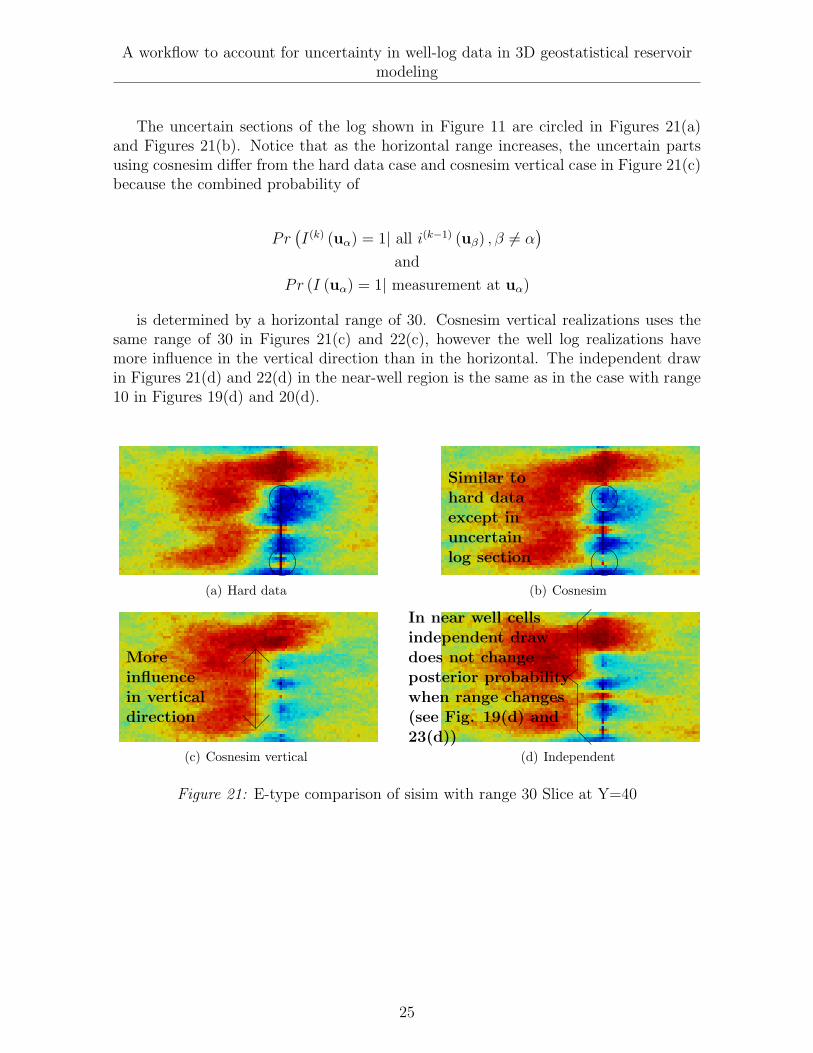
The uncertain sections of the log shown in Figure 11 are circled in Figures 21(a)and Figures 21(b). Notice that as the horizontal range increases, the uncertain partsusing cosnesim differ from the hard data case and cosnesim vertical case in Figure 21(c)because the combined probability of
Pr(I(k) (uα) = 1| all i(k−1) (uβ) , β 6= α
)and
Pr (I (uα) = 1| measurement at uα)
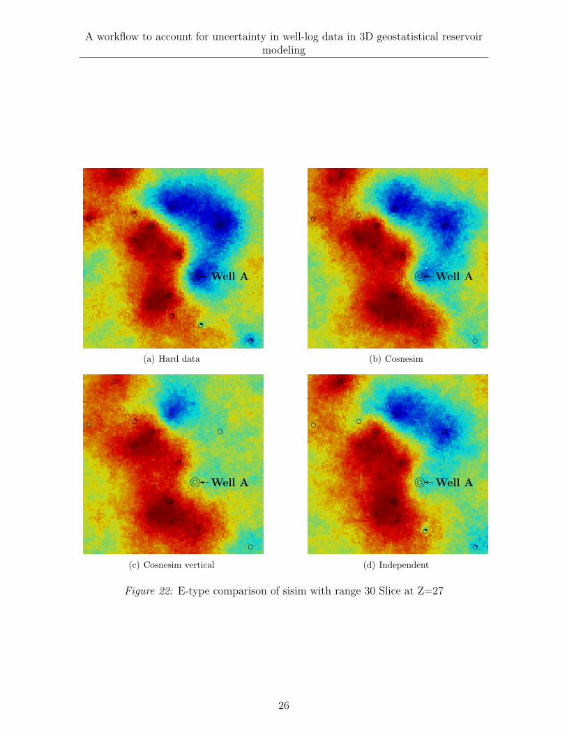
is determined by a horizontal range of 30. Cosnesim vertical realizations uses thesame range of 30 in Figures 21(c) and 22(c), however the well log realizations havemore influence in the vertical direction than in the horizontal. The independent drawin Figures 21(d) and 22(d) in the near-well region is the same as in the case with range10 in Figures 19(d) and 20(d).
(a) Hard data (b) Cosnesim���� �������� ����Similar to
hard dataexcept inuncertainlog section
(c) Cosnesim vertical (d) Independent
�@
@�
Moreinfluencein verticaldirection
�
�Z
@
In near well cellsindependent drawdoes not changeposterior probabilitywhen range changes(see Fig. 19(d) and23(d))
Figure 21: E-type comparison of sisim with range 30 Slice at Y=40
25
A workflow to account for uncertainty in well-log data in 3D geostatistical reservoirmodeling
(a) Hard data (b) Cosnesim
dd
di� Well A
d dd
ddd
dd d
d
d
dd
ddi� Well A
d dd
ddd
dd d
d
d
d
(c) Cosnesim vertical (d) Independent
dd
di� Well A
d dd
ddd
dd d
d
d
dd
ddi� Well A
d dd
ddd
dd d
d
d
d
Figure 22: E-type comparison of sisim with range 30 Slice at Z=27
26
A workflow to account for uncertainty in well-log data in 3D geostatistical reservoirmodeling
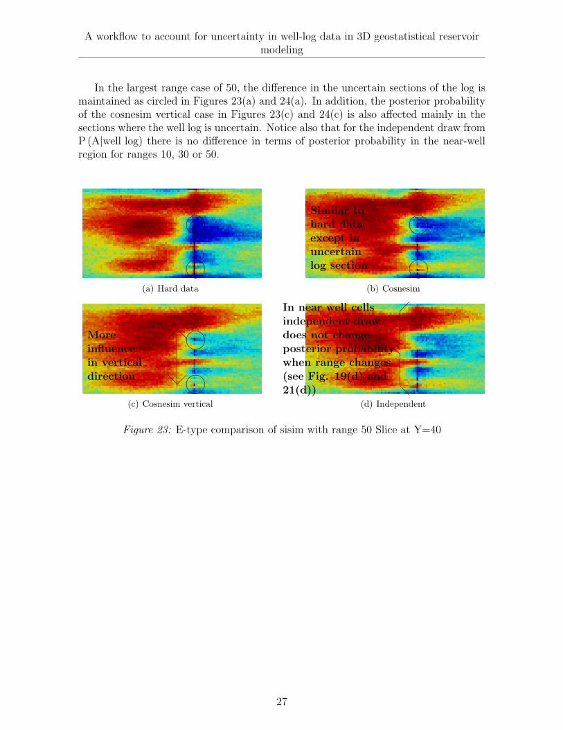
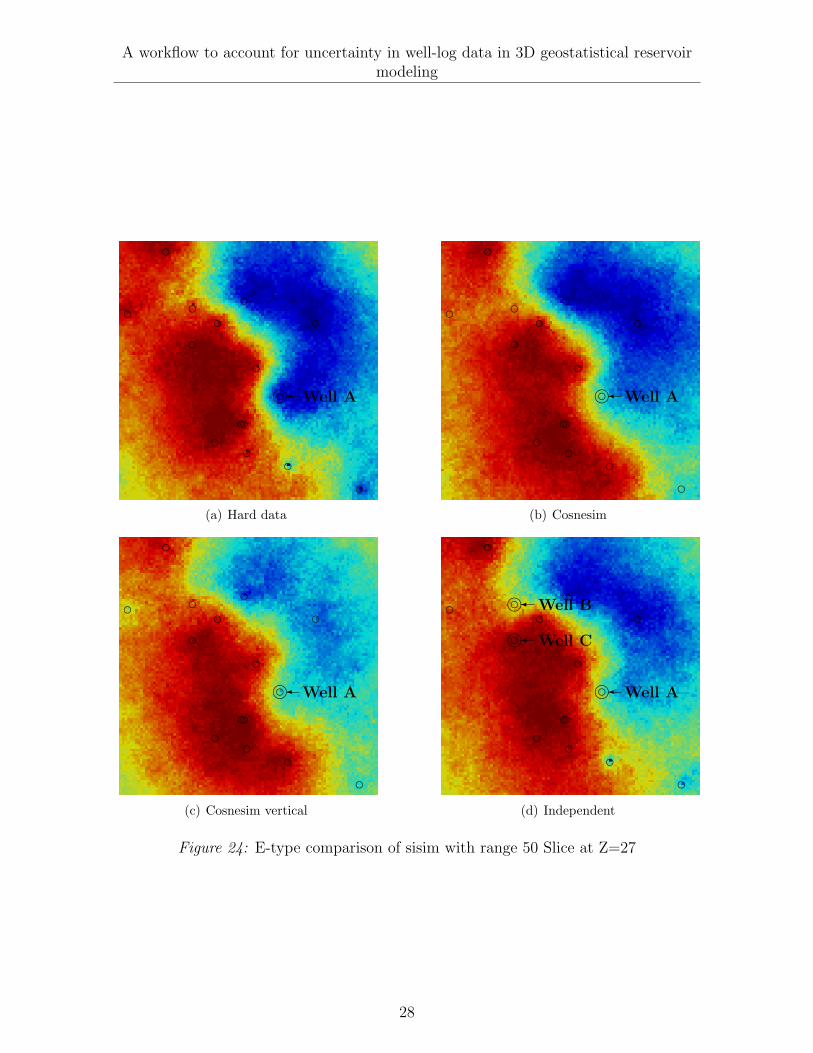
In the largest range case of 50, the difference in the uncertain sections of the log ismaintained as circled in Figures 23(a) and 24(a). In addition, the posterior probabilityof the cosnesim vertical case in Figures 23(c) and 24(c) is also affected mainly in thesections where the well log is uncertain. Notice also that for the independent draw fromP (A|well log) there is no difference in terms of posterior probability in the near-wellregion for ranges 10, 30 or 50.
(a) Hard data (b) Cosnesim���� �������� ����Similar to
hard dataexcept inuncertainlog section
(c) Cosnesim vertical (d) Independent
�@
@�
Moreinfluencein verticaldirection
�
�Z
@
In near well cellsindependent drawdoes not changeposterior probabilitywhen range changes(see Fig. 19(d) and21(d))����
����
Figure 23: E-type comparison of sisim with range 50 Slice at Y=40
27
A workflow to account for uncertainty in well-log data in 3D geostatistical reservoirmodeling
(a) Hard data (b) Cosnesim
dd
di� Well A
d dd
ddd
dd d
d
d
dd
ddi� Well A
d dd
ddd
dd d
d
d
d
(c) Cosnesim vertical (d) Independent
dd
di� Well A
di� Well Bd
d
ddd
ddi� Well C
d
d
d
dd
ddi� Well A
d dd
ddd
dd d
d
d
d
Figure 24: E-type comparison of sisim with range 50 Slice at Z=27
28
A workflow to account for uncertainty in well-log data in 3D geostatistical reservoirmodeling
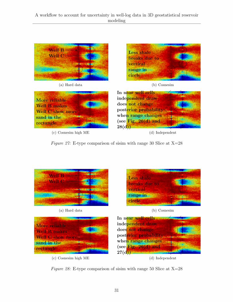
6.1 Effect on near-by wells
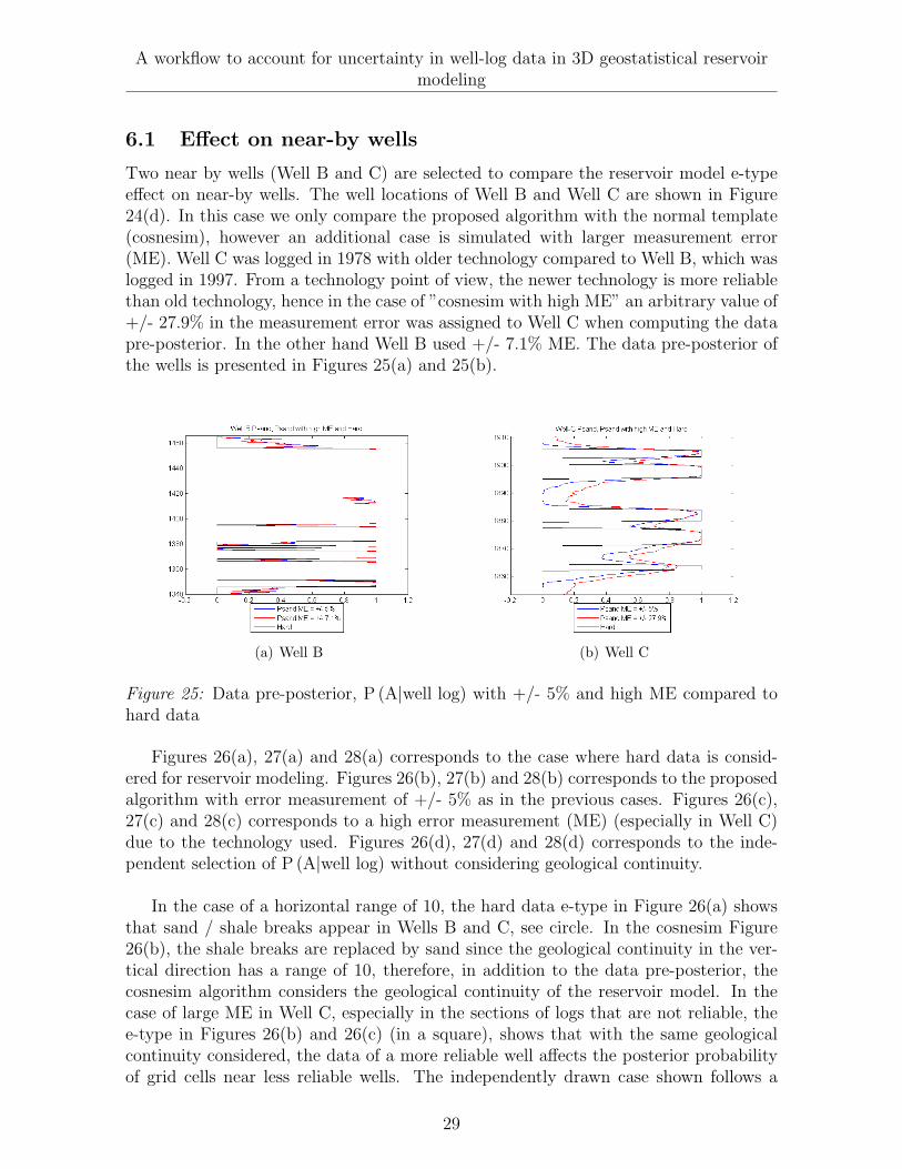
Two near by wells (Well B and C) are selected to compare the reservoir model e-typeeffect on near-by wells. The well locations of Well B and Well C are shown in Figure24(d). In this case we only compare the proposed algorithm with the normal template(cosnesim), however an additional case is simulated with larger measurement error(ME). Well C was logged in 1978 with older technology compared to Well B, which waslogged in 1997. From a technology point of view, the newer technology is more reliablethan old technology, hence in the case of ”cosnesim with high ME” an arbitrary value of+/- 27.9% in the measurement error was assigned to Well C when computing the datapre-posterior. In the other hand Well B used +/- 7.1% ME. The data pre-posterior ofthe wells is presented in Figures 25(a) and 25(b).
(a) Well B (b) Well C
Figure 25: Data pre-posterior, P (A|well log) with +/- 5% and high ME compared tohard data
Figures 26(a), 27(a) and 28(a) corresponds to the case where hard data is consid-ered for reservoir modeling. Figures 26(b), 27(b) and 28(b) corresponds to the proposedalgorithm with error measurement of +/- 5% as in the previous cases. Figures 26(c),27(c) and 28(c) corresponds to a high error measurement (ME) (especially in Well C)due to the technology used. Figures 26(d), 27(d) and 28(d) corresponds to the inde-pendent selection of P (A|well log) without considering geological continuity.
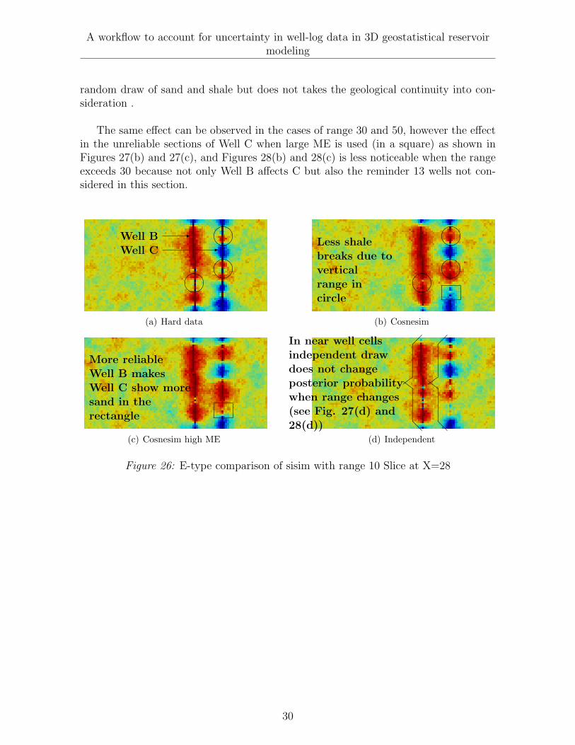
In the case of a horizontal range of 10, the hard data e-type in Figure 26(a) showsthat sand / shale breaks appear in Wells B and C, see circle. In the cosnesim Figure26(b), the shale breaks are replaced by sand since the geological continuity in the ver-tical direction has a range of 10, therefore, in addition to the data pre-posterior, thecosnesim algorithm considers the geological continuity of the reservoir model. In thecase of large ME in Well C, especially in the sections of logs that are not reliable, thee-type in Figures 26(b) and 26(c) (in a square), shows that with the same geologicalcontinuity considered, the data of a more reliable well affects the posterior probabilityof grid cells near less reliable wells. The independently drawn case shown follows a
29
A workflow to account for uncertainty in well-log data in 3D geostatistical reservoirmodeling
random draw of sand and shale but does not takes the geological continuity into con-sideration .
The same effect can be observed in the cases of range 30 and 50, however the effectin the unreliable sections of Well C when large ME is used (in a square) as shown inFigures 27(b) and 27(c), and Figures 28(b) and 28(c) is less noticeable when the rangeexceeds 30 because not only Well B affects C but also the reminder 13 wells not con-sidered in this section.
(a) Hard data (b) Cosnesim
Well BWell C -
-
��������
��������
����
����Less shalebreaks due toverticalrange incircle
(c) Cosnesim high ME (d) Independent
More reliableWell B makesWell C show moresand in therectangle
�
�Z
@
�
�Z
@
In near well cellsindependent drawdoes not changeposterior probabilitywhen range changes(see Fig. 27(d) and28(d))
Figure 26: E-type comparison of sisim with range 10 Slice at X=28
30
A workflow to account for uncertainty in well-log data in 3D geostatistical reservoirmodeling
(a) Hard data (b) Cosnesim
Well BWell C -
-
��������
��������
����
����Less shalebreaks due toverticalrange incircle
(c) Cosnesim high ME (d) Independent
More reliableWell B makesWell C show moresand in therectangle
�
�Z
@
�
�Z
@
In near well cellsindependent drawdoes not changeposterior probabilitywhen range changes(see Fig. 26(d) and28(d))
Figure 27: E-type comparison of sisim with range 30 Slice at X=28
(a) Hard data (b) Cosnesim
Well BWell C -
-
��������
��������
����
����Less shalebreaks due toverticalrange incircle
(c) Cosnesim high ME (d) Independent
More reliableWell B makesWell C show moresand in therectangle
�
�Z
@
�
�Z
@
In near well cellsindependent drawdoes not changeposterior probabilitywhen range changes(see Fig. 26(d) and27(d))
Figure 28: E-type comparison of sisim with range 50 Slice at X=28
31
A workflow to account for uncertainty in well-log data in 3D geostatistical reservoirmodeling
7 Conclusions
A method for modeling uncertainty related to hard data was implemented using 3D realwell data. The method does not require the usual assumptions of co-location, Gaus-sianity or independence, nor does it call for tedious cross-variogram modeling. Instead,an iterative process (cosnesim and cosnesim vertical) are proposed that honors not onlythe uncertain data but also the spatial geological continuity model provided through avariogram model.
The method proposed may overcome the difficulty of integrating sources of differentreliability by means of a data pre-posterior instead of constraining the model with harddata. Providing uncertainty on hard data is often very useful when performing historymatching. Freezing data at wells may render a history match infeasible in real fieldcases (Hoffman (2005)).
The method generates several realizations of hard data sets which can be used in afurther integrated uncertainty analysis by considering other sources of uncertainties.
References
Akamine, J. and Caers, J.: 2006, Conditioning stochastic realizations to hard data withvarying reliability, Report 19, Stanford Center for Reservoir Forecasting, Stanford,CA.
Bassiouni, Z.: 1994, Theory, Measurement, and Interpretation of Well Logs, SPE Text-book Series Vol. 4, Society of Petroleum Engineers, Richardson, TX.
Hoffman, T.: 2005, History matching while perturbing facies, PhD thesis, StanfordUniversity, Stanford, CA.
Journel, A.: 2002, Combining knowledge from diverse sources: An alternative to tradi-tional data independence hypotheses, Mathematical Geology 34(5), 573–596.
Strebelle, S.: 2002, Conditional simulation of complex geological structures usingmultiple-point statistics, Mathematical Geology 34(1), 1–21.
32