A WORKING CLASSIFICATION OF U.S. TERRESTRIAL SYSTEMS Serve's Ecological...ECOLOGICAL SYSTEMS OF THE...
141
ECOLOGICAL SYSTEMS OF THE UNITED STATES A WORKING CLASSIFICATION OF U.S. TERRESTRIAL SYSTEMS
Transcript of A WORKING CLASSIFICATION OF U.S. TERRESTRIAL SYSTEMS Serve's Ecological...ECOLOGICAL SYSTEMS OF THE...

ECOLOGICAL SYSTEMS OF THE UNITED STATES A WORKING CLASSIFICATION OF U.S. TERRESTRIAL SYSTEMS
NatureServe is a non-profit organization dedicated to providing the scientific knowledge that forms the basis for effective conservation action. Citation: Comer, P., D. Faber-Langendoen, R. Evans, S. Gawler, C. Josse, G. Kittel, S. Menard, M. Pyne, M. Reid, K. Schulz, K. Snow, and J. Teague. 2003. Ecological Systems of the United States: A Working Classification of U.S. Terrestrial Systems. NatureServe, Arlington, Virginia. © NatureServe 2003 Ecological Systems of the United States is a component of NatureServe’s International Terrestrial Ecological Systems Classification. � Funding for this report was provided by a grant from The Nature Conservancy. Front cover: Maroon Bells Wilderness, Colorado. Photo © Patrick Comer NatureServe 1101 Wilson Boulevard, 15th Floor Arlington, VA 22209 (703) 908-1800 www.natureserve.org

ECOLOGICAL SYSTEMS OF THE UNITED STATES A WORKING CLASSIFICATION OF U.S. TERRESTRIAL SYSTEMS
�
�
�
�
�
Patrick Comer Don Faber-Langendoen
Rob Evans Sue Gawler
Carmen Josse Gwen Kittel
Shannon Menard Milo Pyne
Marion Reid Keith Schulz Kristin Snow Judy Teague
June 2003

i
Acknowledgements We wish to acknowledge the generous support provided by The Nature Conservancy for this effort to
classify and characterize the ecological systems of the United States. We are particularly grateful to the
late John Sawhill, past President of The Nature Conservancy, who was an early supporter of this concept,
and who made this funding possible through an allocation from the President’s Discretionary Fund.
Many of the concepts and approaches for defining and applying ecological systems have greatly benefited
from collaborations with Conservancy staff, and the classification has been refined during its application
in Conservancy-sponsored conservation assessments. In addition, we appreciate the support and insights
provided by Leni Wilsmann, the Conservancy’s liaison to NatureServe.
Throughout this effort, numerous individuals contributed directly through workshops, working groups,
and expert review. We wish to express our sincere appreciation to the following natural heritage program
ecologists and their close working partners. The expertise and ecological data provided by this network of
scientists helped form the basis for this classification.
Peter Achuff Lorna Allen Craig Anderson Mark Anderson Keith Boggs Bob Campbell Chris Chappell Steve Cooper Rex Crawford Robert Dana Hannah Dunevitz Lee Elliot Eric Epstein Julie Evens Tom Foti Ann Gerry
Jason Greenall Dennis Grossman Mary Harkness Bruce Hoagland George Jones Jimmy Kagan Todd Keeler-Wolf Steve Kettler Kelly Kindscher Del Meidinger Gerald Manis Larry Master Larry Morse Esteban Muldavin Jan Nachlinger Tim Nigh
Carl Nordman Chris Pague Carol Reschke Renee Rondeau Mary Russo Mike Schafale Dan Sperduto Gerry Steinauer Rick Schneider Terri Schulz Leslie Sneddon Joel Tuhy Kathryn Thomas Jim Vanderhorst Peter Warren Alan Weakley
ii
Table of Contents
i
Acknowledgements ....................................................................................................................................... i
Executive Summary..................................................................................................................................... iv
Introduction and Background ....................................................................................................................... 1
Key Issues and Decisions in Developing Ecological Systems ..................................................................... 5
Ecological Systems as Functional Units versus Landscape Units............................................................ 5
Ecological Systems as Geo-Systems versus Bio-Systems.......................................................................... 6
Ecological Systems as Discrete Units versus Individualistic Units .......................................................... 7
The Scale of Ecological Systems............................................................................................................... 8
Terrestrial Ecological Systems: Conceptual Basis ..................................................................................... 10
Meso-Scale Ecosystems........................................................................................................................... 11
Diagnostic Classifiers ............................................................................................................................. 12
Methods of Classification Development .................................................................................................... 17
Classification Structure........................................................................................................................... 17
Development of Diagnostic Criteria and Descriptions .................................................................................. 18
Pattern Type............................................................................................................................................ 20
Nomenclature for Ecological Systems .................................................................................................... 21
Results ........................................................................................................................................................ 23
Number and Distribution of Systems....................................................................................................... 23
Linking System Types to Land Cover Types............................................................................................ 26
Data Management and Access................................................................................................................ 27
Applications................................................................................................................................................ 29
Applications to Conservation Assessment............................................................................................... 29
Applications to Element Occurrence Inventory and Mapping................................................................ 31
Applications to Comprehensive Mapping ............................................................................................... 34
Applications to Management and Monitoring ........................................................................................ 42
Applications to Habitat Modeling........................................................................................................... 48

iii
Avenues for Classification Refinement ...................................................................................................... 49
Conclusions ................................................................................................................................................ 51
Literature Cited........................................................................................................................................... 52
Appendices ................................................................................................................................................. 61
Appendix 1. Existing Classification Systems........................................................................................... 61
Appendix 2. Element Occurrence Specifications .................................................................................... 67
Appendix 3. NatureServe Global Conservation Status Definitions......................................................... 72
Appendix 4. Terrestrial Ecological Systems and Wildlife Habitats in California .................................. 73
List of Tables
Table 1. Categories for patch types used to describe ecological systems.................................................. 21 Table 2. Breakdown of ecological system types in terms of prevailing vegetation physiognomy and
upland/wetland status, closely matching categories mapped in National Land Cover Data. ............. 27 Table 3. Core Selection Criteria for Elements for Biodiversity Conservation .......................................... 30 Table 4. Recommended Minimum Separation Distances for Communities and Ecological Systems....... 34 Table 5. Basic Element Occurrence Ranks................................................................................................ 43 Table 6. Rank Attribute Categories and Key Ecological Attributes.......................................................... 44 Table 7. Partial EO Rank document for the Northern California Hardpan Vernal Pool modified from
the Consumnes River Preserve Plan of The Nature Conservancy of California. ............................... 47
List of Figures Figure 1. Project Area included in this classification effort. ...................................................................... 4 Figure 2. Ecological Divisions of North America used in organization and nomenclature of .................. 14 NatureServe Ecological Systems. Project area of this report is highlighted............................................. 14 Figure 3. Sample decision matrix for classification of selected ecological systems found in the
Laurentian-Acadian Ecological Division. .......................................................................................... 19 Figure 4. Number of Terrestrial Ecological System types by Ecological Division. ................................... 24 Figure 5. Number of Terrestrial Ecological System types by Ecoregion. .................................................. 25 Figure 6. Number of Terrestrial Ecological System types by State. ........................................................... 26 Figure 7. Alliance-scale units mapped comprehensively across CO, KS, NE, SD, and WY ..................... 36 Figure 8. Terrestrial ecological system-scale units mapped comprehensively across CO, KS, NE, SD,
and WY (from Comer et al. 2003)....................................................................................................... 38 Figure 9. Terrestrial ecological systems of Zion National Park and environs .......................................... 40 Figure 10. Rank scale for “A”, “B”, “C”, and “D”-ranked EOs. ............................................................ 45

iv
Executive Summary Conservation of the Earth’s diversity of life requires a sound understanding of the distribution and
condition of the components of that diversity. Efforts to understand our natural world are directed at a
variety of biological and ecological scales—from genes and species, to natural communities, local
ecosystems, and landscapes. While scientists have made considerable progress classifying fine-grained
ecological communities on the one hand, and coarse-grained ecoregions on the other, land managers have
identified a critical need for practical, mid-scale ecological units to inform conservation and resource
management decisions. This report introduces and outlines the conceptual basis for such a mid-scale
classification unit—ecological systems.
Ecological systems represent recurring groups of biological communities that are found in similar
physical environments and are influenced by similar dynamic ecological processes, such as fire or
flooding. They are intended to provide a classification unit that is readily mappable, often from remote
imagery, and readily identifiable by conservation and resource managers in the field.
NatureServe and its natural heritage program members, with funding from The Nature Conservancy,
have completed a working classification of terrestrial ecological systems in the coterminous United
States, southern Alaska, and adjacent portions of Mexico and Canada. This report summarizes the nearly
600 ecological systems that currently are classified and described. We document applications of these
ecological systems for conservation assessment, ecological inventory, mapping, land management,
ecological monitoring, and species habitat modeling.
Terrestrial ecological systems are specifically defined as a group of plant community types
(associations) that tend to co-occur within landscapes with similar ecological processes, substrates, and/or
environmental gradients. A given system will typically manifest itself in a landscape at intermediate
geographic scales of tens to thousands of hectares and will persist for 50 or more years. This temporal
scale allows typical successional dynamics to be integrated into the concept of each unit. With these
temporal and spatial scales bounding the concept of ecological systems, we then integrate multiple
ecological factors—or diagnostic classifiers—to define each classification unit. The multiple ecological
factors are evaluated and combined in different ways to explain the spatial co-occurrence of plant
associations.
Summarizing across the range of natural variation, some 381 ecological systems (63%) are upland
types, 183 (31%) are wetland types, and 35 (6%) are complexes of uplands and wetlands. Considering
prevailing vegetation structure, 322 systems (54%) are predominantly forest, woodland, or shrubland, 166
systems (28%) are predominantly herbaceous, savanna, or shrub steppe, and 74 systems (12%) are
sparsely vegetated or “barren.”

v
Terrestrial ecological system units represent practical, systematically defined groupings of plant
associations that provide the basis for mapping terrestrial communities and ecosystems at multiple scales
of spatial and thematic resolution. The systems approach complements the U.S. National Vegetation
Classification, whose finer-scale units provide a basis for interpreting larger-scale ecological system
patterns and concepts. The working classification presented in this report will serve as the basis for
NatureServe to facilitate the ongoing development and refinement of the U.S. component of an
International Terrestrial Ecological Systems Classification.

Ecological Systems of the United States 1
Introduction and Background Attempts to understand and conserve our natural world have often been directed at different
biological and ecological levels, from genes and species, to communities, local ecosystems, and
landscapes. Ecological conservation and resource managers typically require the identification,
description, and assessment of some or all levels of biodiversity within a given planning area or
ecoregion. Practically speaking, the focal elements that define these levels need to be clearly specified to
clarify exactly what is to be protected or managed (Groves et al. 2002).
Conservationists and resource managers now use a variety of approaches to assess biodiversity at
different scales (Redford et al. 2003). Species and ecoregions have received a great deal of attention.
Species approaches include a focus on rare or endemic species, focal or umbrella species, and biodiversity
hot spots. Ecoregional approaches include global prioritizations, such as the WWF Global 2000
ecoregions (Redford et al. 2003) or ecological land classifications (e.g., Albert 1995, Bailey 1996).
Community and local ecosystem approaches have been less-well developed, though community
approaches have been commonly used by natural heritage programs at the state level (e.g. Schafale and
Weakley 1990, Reschke 1990). With the development of national and international vegetation
classifications (Grossman et al. 1998, Rodwell et al. 2002, Jennings et al. 2003), the community approach
is now applicable at more extensive geographic scales, at multiple levels of resolution. The local
ecosystem approach has included mapping and assessment of fine-scaled landscape ecosystem units (e.g.
see Barnes et al. 1998) or the definition of ecological system units within ecoregions (e.g. Neely et al
2001, Tuhy et al. 2002).
A common set of concerns for conservation or resource managers are: a) the spatial scale of the focal
element (the “grain”); b) the degree of consistency in the element definition or taxonomy; c) the extent to
which they can be applied across multiple jurisdictions or even continents; and d) the extent to which
information can be readily assembled to assess their distribution, status, and trends. The species approach
may require that grain be assessed on a species-by-species basis. The degree of consistency is improving
as taxonomies improve, but parts of the world are not well surveyed. Worldwide lists and red lists are
increasingly available, but information on many species is often difficult to obtain.
Ecoregional approaches often provide multiple levels of spatial scales, but typically the grain is quite
coarse, and the units are unique subsets of the geographic space, with varying degrees of heterogeneity.
They are either used as focal elements directly or as organizing units for focusing on more specific focal
elements within the region. They are now increasingly available around the world, and information can
be readily assembled, depending on the features of the ecoregion being assessed.
Community approaches, often considered a more convenient focal element (the “coarse filter’), as
compared to species (the “fine filter”) (Jenkins 1976), often have a fine grain, are relatively consistent,

2 NatureServe
but are often not feasibly applied to national or broader assessments (e.g. Noss and Peters 1995). Their
fine grain may hinder ability to assemble information and conduct assessment, limiting their practical
value. Our experience in the application of the International Vegetation Classification (IVC) and its U.S.
component, the U.S. National Vegetation Classification1 (NVC) has indicated the need for standardized
classification units that more fully integrate environmental factors into unit definition (e.g. Anderson et al.
1999). There is also a need to define units somewhat more broadly than individual NVC floristic units
(alliances and associations) – i.e., allowing for a greater range of biotic and abiotic heterogeneity in type
definition – without “scaling up” to the NVC formation unit, which is defined solely through vegetation
physiognomy and limited environmental factors.
Finally, the intermediate-scaled landscape ecosystems (e.g. USFS ECOMAP Land Type
Associations) are often difficult to define consistently, and may be rather heterogeneous with respect to
biodiversity. They are not fully developed or widely available across the country, or across continents,
making it difficult to use these units in regional, national, or international assessments.
Lacking in these approaches is a focal element that is more coarsely grained than the community
approach, retains a standard of consistency that allows ready identification and application of the unit at
local or regional scales, and that is widely applicable at continental or hemispheric levels. In addition,
gathering information on such focal elements should not make excessive information demands on
conservation or resource managers. Here we describe a standardized terrestrial ecological system
classification designed to meet these objectives. Our purpose is to demonstrate that these systems, though
related to both community and landscape ecosystem approaches, provide a greatly improved set of focal
elements for conservation and resource management.
Ecological Scope of Classification. The emphasis of this classification is directed towards surficial
terrestrial environments, encompassing both upland and wetland areas where rooted and non-vascular
vegetation – as well as readily identifiable environmental features (e.g. alpine, coastal, cliff, sand dune,
river floodplain, depressional wetland, etc.) - may be used to recognize and describe each type. We do
not address either subterranean environments, or aquatic environments, whether freshwater or marine.
Within terrestrial environments, we focus here on existing ecological system types that can be considered
“natural” or “near-natural,” i.e., those that appear to be unmodified or only marginally impacted by human
activities. This is to provide a framework for describing ecological composition, structure, and function that
has existed with minimal human influence under climatic regimes of recent millennia. We have made no
attempt to classify and describe agricultural ecosystems or urban ecosystems where human-caused elements
1 See Appendix 1 for further explanation of the U.S. National Vegetation Classification as well as other existing classification approaches.

Ecological Systems of the United States 3
are clearly novel in a temporal context of 100s to 1000s of years. Instead, as we apply this classification to
mapping, we rely on broadly based land cover classes to identify and map human-dominated areas. With
this approach, we are still able to track the current status of natural ecosystems relative to cultural ones, and
even suggest how human alterations may be viewed more directly in light of presumed historical conditions.
Geographic Scope of Classification. NatureServe is currently working toward a first-draft classification
of terrestrial ecological systems across North and South America –an International Terrestrial Ecological
Systems Classification. A team of NatureServe and natural heritage program ecologists has now
completed a working list and descriptions of the U.S. Terrestrial Ecological Systems Classification, which
includes nearly 600 terrestrial ecological systems in the coterminous, lower 48 United States, portions of
southern coastal Alaska, and ecologically similar regional landscapes in adjacent southern Canada and
northern Mexico (Figure 1). Their distribution by ecoregions, as defined by The Nature Conservancy
(Groves et al. 2002), is also documented, thereby providing a list of focal elements that can facilitate
conservation work in that organization.
The Iterative Nature of Classification. Ecological classifications, such as this one, should be viewed as
an ongoing process of stating assumptions, data gathering, data analysis and synthesis, testing new
knowledge through field application, and classification refinement. A classification system provides a
framework for this ongoing process and the resulting classification should continually change as new
knowledge is gained. The effort documented here represents the first attempt to synthesize data and apply
a standard approach to documenting natural upland and wetland ecological systems comprehensively
across the coterminous United States. Although in this report we include adjacent regions based on the
ecoregional boundaries that extend beyond the U.S., additional collaboration with partners is needed to
advance this classification internationally. NatureServe will continue to provide a mechanism for
ongoing development and dissemination of this classification.
Objectives of This Report. This report documents the development of terrestrial ecological systems,
emphasizing the key issues and requirements of such a system in relation to other approaches. We review
the criteria used to classify systems and the standards that were used to develop, name, and describe them.
We describe the process for gathering information on these systems and summarize the results of this
initial classification effort. We then describe the application of ecological system units for mapping and
assessing occurrence quality or ecological integrity. We also describe the application of these units to
conservation assessment and description of wildlife habitat. Finally we address the next steps in the
process of further enhancing the systems classification.

4 NatureServe
Figure 1. Project Area included in this classification effort.

Ecological Systems of the United States 5
Key Issues and Decisions in Developing Ecological Systems Ecosystems have been defined generally as “ a community of organisms and their physical
environment interacting as an ecological unit” (Lincoln et al. 1982). Classification of ecological systems
can be based on a variety of factors (e.g., vegetation, soils, landforms) at a variety of spatial and temporal
scales (hectares to millions of kilometers and annual to millennial), and with varying degrees of concern
over spatial interactions. A full review of the variety of classifications currently used is beyond the scope
of this document. Rather, some key issues will be highlighted that includes discussions of other
approaches. See Appendix 1 for a review of some major classifications that informed our approach.
Ecological Systems as Functional Units versus Landscape Units Historically, ecological systems have been defined from a wide variety of perspectives, depending on
the investigator. Some have emphasized the “physical” (land) factors that structure the system; others
have emphasized ecosystem function and processes, such as nutrient cycling and energy flows (Golley
1993). Odum (2001) emphasizes the latter perspective in his definition of ecological system:
An ecological system, or ecosystem, is any unit (a biosystem) that includes all the organisms (the
biotic community) in a given area interacting with the physical environment so that a flow of energy
leads to clearly defined biotic structures and cycles of materials between living and non-living parts.
An ecosystem is more than a geographic unit (or ecoregion); it is a functional system with inputs and
outputs, and with boundaries that can be neither natural or arbitrary.
The emphasis is on energy flow and nutrient cycling, looking at how primary and secondary
producers shape the flow of energy and materials through a system. By contrast, Bailey (1996)
emphasizes the landscape ecosystem approach:
J. S. Rowe … defined an ecosystem as “a topographic unit, a volume of land and air plus organic
contents extending areally over a particular part of the earth’s surface for a certain time.” This
definition stresses the reality of ecosystems as geographic units of the landscape that include all natural
phenomena and that can be identified and surrounded by boundaries.”
These definitions do not lead to mutually exclusive approaches to ecosystem studies. Many
functional studies use watershed geographic units to define their ecosystems; and landscape ecosystem
studies often emphasize functional properties within and across geographic units. Our decision was to
emphasize a classification approach to ecosystems that does not rely on a fixed landscape map unit and
which is still amenable to process-functional studies. We emphasize how processes on the landscape
shape ecological systems, and define them through a combination of biotic and abiotic criteria.
6 NatureServe
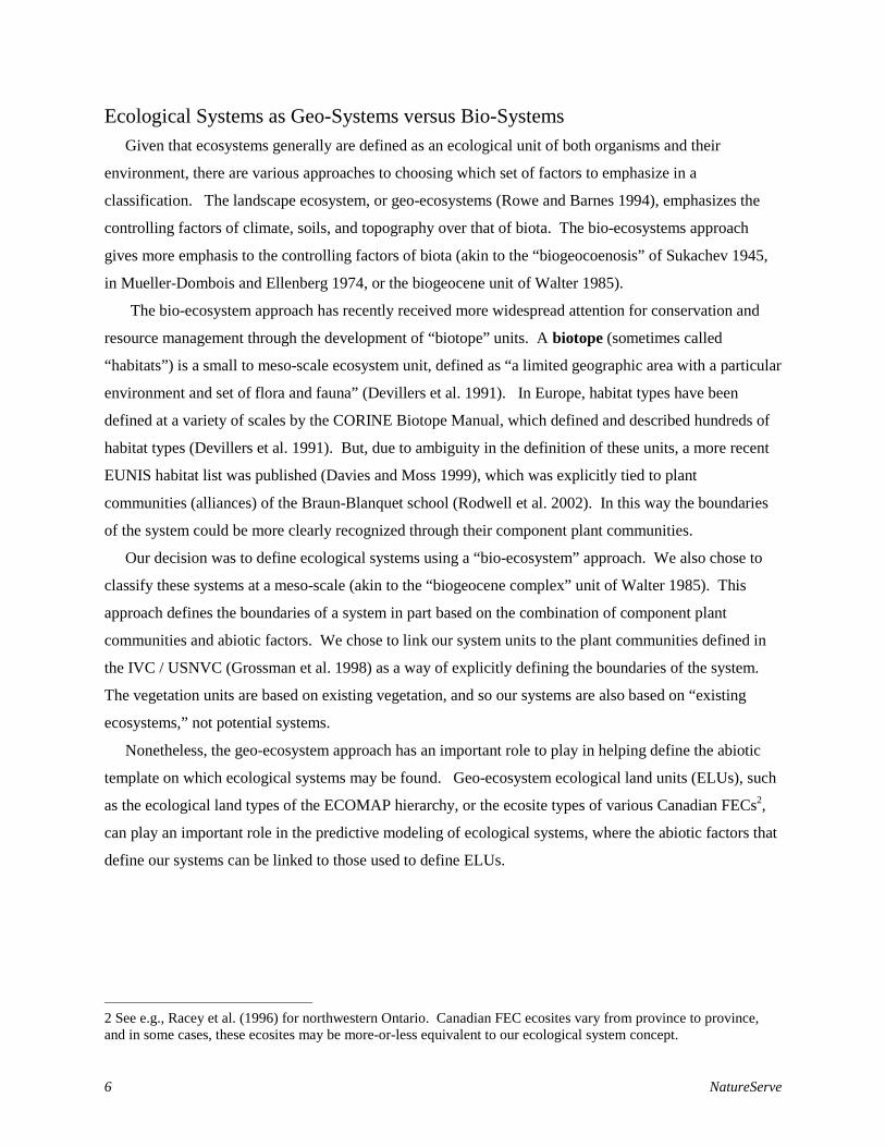
Ecological Systems as Geo-Systems versus Bio-Systems Given that ecosystems generally are defined as an ecological unit of both organisms and their
environment, there are various approaches to choosing which set of factors to emphasize in a
classification. The landscape ecosystem, or geo-ecosystems (Rowe and Barnes 1994), emphasizes the
controlling factors of climate, soils, and topography over that of biota. The bio-ecosystems approach
gives more emphasis to the controlling factors of biota (akin to the “biogeocoenosis” of Sukachev 1945,
in Mueller-Dombois and Ellenberg 1974, or the biogeocene unit of Walter 1985).
The bio-ecosystem approach has recently received more widespread attention for conservation and
resource management through the development of “biotope” units. A biotope (sometimes called
“habitats”) is a small to meso-scale ecosystem unit, defined as “a limited geographic area with a particular
environment and set of flora and fauna” (Devillers et al. 1991). In Europe, habitat types have been
defined at a variety of scales by the CORINE Biotope Manual, which defined and described hundreds of
habitat types (Devillers et al. 1991). But, due to ambiguity in the definition of these units, a more recent
EUNIS habitat list was published (Davies and Moss 1999), which was explicitly tied to plant
communities (alliances) of the Braun-Blanquet school (Rodwell et al. 2002). In this way the boundaries
of the system could be more clearly recognized through their component plant communities.
Our decision was to define ecological systems using a “bio-ecosystem” approach. We also chose to
classify these systems at a meso-scale (akin to the “biogeocene complex” unit of Walter 1985). This
approach defines the boundaries of a system in part based on the combination of component plant
communities and abiotic factors. We chose to link our system units to the plant communities defined in
the IVC / USNVC (Grossman et al. 1998) as a way of explicitly defining the boundaries of the system.
The vegetation units are based on existing vegetation, and so our systems are also based on “existing
ecosystems,” not potential systems.
Nonetheless, the geo-ecosystem approach has an important role to play in helping define the abiotic
template on which ecological systems may be found. Geo-ecosystem ecological land units (ELUs), such
as the ecological land types of the ECOMAP hierarchy, or the ecosite types of various Canadian FECs2,
can play an important role in the predictive modeling of ecological systems, where the abiotic factors that
define our systems can be linked to those used to define ELUs.
2 See e.g., Racey et al. (1996) for northwestern Ontario. Canadian FEC ecosites vary from province to province, and in some cases, these ecosites may be more-or-less equivalent to our ecological system concept.
Ecological Systems of the United States 7
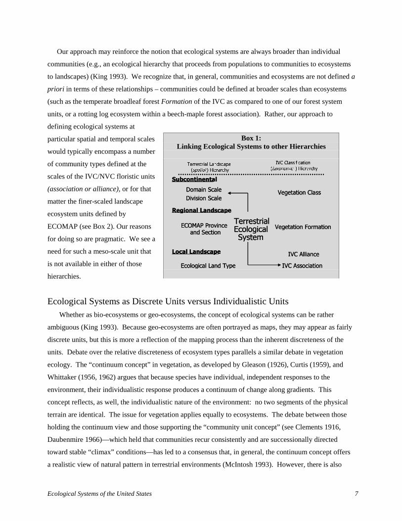
Our approach may reinforce the notion that ecological systems are always broader than individual
communities (e.g., an ecological hierarchy that proceeds from populations to communities to ecosystems
to landscapes) (King 1993). We recognize that, in general, communities and ecosystems are not defined a
priori in terms of these relationships – communities could be defined at broader scales than ecosystems
(such as the temperate broadleaf forest Formation of the IVC as compared to one of our forest system
units, or a rotting log ecosystem within a beech-maple forest association). Rather, our approach to
defining ecological systems at
particular spatial and temporal scales
would typically encompass a number
of community types defined at the
scales of the IVC/NVC floristic units
(association or alliance), or for that
matter the finer-scaled landscape
ecosystem units defined by
ECOMAP (see Box 2). Our reasons
for doing so are pragmatic. We see a
need for such a meso-scale unit that
is not available in either of those
hierarchies.
Ecological Systems as Discrete Units versus Individualistic Units Whether as bio-ecosystems or geo-ecosystems, the concept of ecological systems can be rather
ambiguous (King 1993). Because geo-ecosystems are often portrayed as maps, they may appear as fairly
discrete units, but this is more a reflection of the mapping process than the inherent discreteness of the
units. Debate over the relative discreteness of ecosystem types parallels a similar debate in vegetation
ecology. The “continuum concept” in vegetation, as developed by Gleason (1926), Curtis (1959), and
Whittaker (1956, 1962) argues that because species have individual, independent responses to the
environment, their individualistic response produces a continuum of change along gradients. This
concept reflects, as well, the individualistic nature of the environment: no two segments of the physical
terrain are identical. The issue for vegetation applies equally to ecosystems. The debate between those
holding the continuum view and those supporting the “community unit concept” (see Clements 1916,
Daubenmire 1966)—which held that communities recur consistently and are successionally directed
toward stable “climax” conditions—has led to a consensus that, in general, the continuum concept offers
a realistic view of natural pattern in terrestrial environments (McIntosh 1993). However, there is also
Box 1: Linking Ecological Systems to other Hierarchies
��������������
������������
�����������
����������������� �� � ������� �����������
������������
�������������� ���������
����������� ������� ������
������������������ � ������� �����������
��������������
�������������
����������
���������������
������������������
��������� ��������������
������������
�����������
����������������� �� � ������� �����������
������������
�������������� ���������
����������� ������� ������
������������������ � �����������
��������������
�������������
����������
���������������
������������������
���������
8 NatureServe
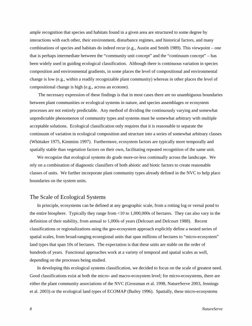
ample recognition that species and habitats found in a given area are structured to some degree by
interactions with each other, their environment, disturbance regimes, and historical factors, and many
combinations of species and habitats do indeed recur (e.g., Austin and Smith 1989). This viewpoint – one
that is perhaps intermediate between the “community unit concept” and the “continuum concept” – has
been widely used in guiding ecological classification. Although there is continuous variation in species
composition and environmental gradients, in some places the level of compositional and environmental
change is low (e.g., within a readily recognizable plant community) whereas in other places the level of
compositional change is high (e.g., across an ecotone).
The necessary expression of these findings is that in most cases there are no unambiguous boundaries
between plant communities or ecological systems in nature, and species assemblages or ecosystem
processes are not entirely predictable. Any method of dividing the continuously varying and somewhat
unpredictable phenomenon of community types and systems must be somewhat arbitrary with multiple
acceptable solutions. Ecological classification only requires that it is reasonable to separate the
continuum of variation in ecological composition and structure into a series of somewhat arbitrary classes
(Whittaker 1975, Kimmins 1997). Furthermore, ecosystem factors are typically more temporally and
spatially stable than vegetation factors on their own, facilitating repeated recognition of the same unit.
We recognize that ecological systems do grade more-or-less continually across the landscape. We
rely on a combination of diagnostic classifiers of both abiotic and biotic factors to create reasonable
classes of units. We further incorporate plant community types already defined in the NVC to help place
boundaries on the system units.
The Scale of Ecological Systems In principle, ecosystems can be defined at any geographic scale, from a rotting log or vernal pond to
the entire biosphere. Typically they range from <10 to 1,000,000s of hectares. They can also vary in the
definition of their stability, from annual to 1,000s of years (Delcourt and Delcourt 1988). Recent
classifications or regionalizations using the geo-ecosystem approach explicitly define a nested series of
spatial scales, from broad-ranging ecoregional units that span millions of hectares to “micro-ecosystem”
land types that span 10s of hectares. The expectation is that these units are stable on the order of
hundreds of years. Functional approaches work at a variety of temporal and spatial scales as well,
depending on the processes being studied.
In developing this ecological systems classification, we decided to focus on the scale of greatest need.
Good classifications exist at both the micro- and macro-ecosystem level; for micro-ecosystems, there are
either the plant community associations of the NVC (Grossman et al. 1998, NatureServe 2003, Jennings
et al. 2003) or the ecological land types of ECOMAP (Bailey 1996). Spatially, these micro-ecosystems

Ecological Systems of the United States 9
are usually defined at scales of 10s to 1,000s of hectares. Temporally the associations typically reflect
vegetation stability at scales of 10 to 100 or more years; the ecological land type also typically emphasize
soil-landform stability at the scale of 50 to 100s of years. At macro-ecosystem scales, vegetation
formations (UNESCO 1973, FGDC 1997, Grossman et al. 1998) or ecoregions (Bailey 1996) can be used.
Spatially, these macro-systems often span continents. Temporally, formations vary in their stability
(though recognition tends to focus on the more stable units), and ecoregions emphasize stability on the
order of 100s to 1000s of years.
Notably lacking, however, are good meso-scale units. For bio-ecosystems that rely on plant
communities, the change in scale between formations and alliance units is rather large. Experience in
application of the NVC has indicated the need for units that are somewhat more broadly defined than
individual NVC alliance and association units – i.e. allowing for a greater range of biotic and abiotic
heterogeneity in type definition – without “scaling up” to the NVC formation unit, which is defined solely
through vegetation physiognomy and limited environmental factors. For geo-ecosystems, the meso-scale
units of subsections and land type association units are still in development, and standards are still lacking
across the country (Smith 2002).
Thus, our decision was to focus on meso-scale ecological system units. The problem we are
addressing is not new. Walter (1985, p. 17) stated:
Between the biomes on the one hand and the biogeocenes [corresponding to the plant community
with the rank of an association], on the other, is a wide gap, which has to be filled by units of
intermediary rank. These units we propose to call biogeocene complexes. They often correspond to a
particular kind of landscape, have a common origin, or are connected with one another by dynamic
processes. As an example, we can cite a biogeocene sequence on a slope with lateral material
transport (catena) or a natural succession of biogeocenes in a river valley or a basin with no
outlet…The different types have as yet been given no ecological names of their own…
In conclusion, our approach to classifying ecological systems draws from a variety of previous efforts
to define ecological units, whether as plant community types or ecological land types. We determined
that a consistent meso-scale ecosystem that could span the North and South American continents was
missing from available classification approaches. We focused our efforts on developing such a unit, one
that could address basic patterns of ecological variability and serve to guide conservation and resource
management needs.
10 NatureServe
Terrestrial Ecological Systems: Conceptual Basis A terrestrial ecological system is defined as a group of plant community types that tend to co-occur
within landscapes with similar ecological processes, substrates, and/or environmental gradients. A given
terrestrial ecological system will typically manifest itself at intermediate geographic scales of 10s to
1,000s of hectares and persist for 50 or more years.
Ecological processes include natural disturbances such as fire and flooding. Substrates may include a
variety of soil surface and bedrock features, such as shallow soils, alkaline parent materials,
sandy/gravelling soils, or peatlands. Finally, environmental gradients include local climates,
hydrologically defined patterns in coastal zones, arid grassland or desert areas, or montane, alpine or
subalpine zones.
By plant community type, we mean a vegetation classification unit at the association or alliance level,
where these are available in the International Vegetation Classification (IVC) and its U.S. component, the
USNVC (NVC) (Grossman et al. 1998, Jennings et al. 2003, NatureServe 2003), or, if these are not
available, other comparable vegetation units. NVC associations are used wherever possible to describe
the component biotic communities of each terrestrial system. The NVC provides a multi-tiered, nested
hierarchy for classifying vegetation types. Currently the NVC includes over 5,000 vegetation
associations and 1,800 vegetation alliances described for the coterminous United States.
Ecological systems are defined using both spatial and temporal criteria that influence the grouping of
associations. Associations that consistently co-occur on the landscape therefore define biotic components
of each ecological system type. Our approach to ecological systems definition using IVC associations is
similar to the biotope or habitat approach used, for example, by the EUNIS habitat classification, which
explicitly links meso-scale habitat units to European Vegetation Survey alliance units (Rodwell et al.
2002). Given the relative ease of recognizing vegetation structure and composition, this approach is
preferable to defining biotic components using animal species that are more difficult to consistently
observe and identify.
In developing an ecological systems approach, we are mindful that ecological systems can be defined
in a number of ways. Indeed, there are so many different definitions that some have suggested that the
concept is in danger of losing its utility. O’Neill (2001) made a number of suggestions to help improve
the ecosystem concept: that the ecosystem (1) be explicitly scaled, (2) include variability, (3) consider
long-term sustainability in addition to local stability, and (4) include population processes as explicit
system dynamics. We define our ecological system concept as follows:

Ecological Systems of the United States 11
1. We explicitly scale the unit to represent, in most cases:
a. spatial scales of tens to thousands of hectares
b. temporal scales of 50 to 100 years
2. We make explicit the variability in the system by describing them in terms of a consistent list of
abiotic and biotic criteria and by linking ecological systems to plant community types
(associations and alliances of the NVC) that describe the biotic community variation within the
system.
3. We propose to consider long-term sustainability and local stability by mapping and evaluating the
occurrence of ecological systems at the local site and the regional level.
4. We do not formally include population processes as explicit system dynamics, but through
knowledge of the component plant communities, we are at least able to describe the major plant
species and their dynamics within the systems. Additional work could formalize the roles of
additional biotic elements such as invertebrates and vertebrates.
Meso-Scale Ecosystems Our concept of terrestrial ecological systems includes temporal and geographic scales intermediate
between stand and landscape-scale analyses. These “meso-scales” constrain the definition of system types
to scales that are of prime interest for conservation and resource managers who are managing landscapes
in the context of a region or state. More precise bounds on both temporal and geographic scales take into
account specific attributes of the ecological patterns that characterize a given region.
Temporal Scale: Within the concept of each classification unit, we clearly acknowledge the dynamic
nature of ecosystems over short and long-term time frames. If we assumed that characteristic
environmental settings (e.g. landform, soil type) remain constant over the time period that applies to
ecological systems (fifty to several hundred years), we would still encounter considerable within-system
variation in vegetation due to disturbance and successional processes. Our temporal scale determines the
means by which we account for both successional changes and disturbance regimes in each classification
unit. Relatively rapid successional changes resulting from disturbances are encompassed within the
concept of a given system unit. Therefore, daily tidal fluctuations will be encompassed within a system
type. Some of the associations describing one system may represent multiple successional stages. For
example, a given floodplain system may include both early successional associations and later mature
woodland stages that form dynamic mosaics along many kilometers of a river. Many vegetation mosaics
resulting from annual to decadal changes in coastal shorelines will be encompassed within a system type.
Many forest and grassland systems will encompass common successional pathways that occur over 20-50
12 NatureServe
year periods. Selecting this temporal scale shares some aspects with the “habitat type” approach to
describe potential vegetation (Daubenmire 1952, Pfister and Arno 1980), but differs in that no “climax”
vegetation is implied, and all seral components are explicitly included in the system concept.
Of course, many environmental attributes, such as climate, continually change over much longer and
more varied time frames. Our concept for any “natural/near-natural” ecological system type encompasses
temporal variation that is responding to climatic variations that have occurred in recent millennia, with
little or no human influence.
Pattern and Geographic Scale: Spatial patterns that we observe at “intermediate” scales can often be
explained by landscape attributes that control the location and dynamics of moisture, nutrients, and
disturbance events. For example, throughout temperate latitudes one can often see distinctions in
vegetation occupying south-facing vs. north-facing slopes or from ridge top to valley bottom. Site factors
in turn may interact with insect, disease, and fire. Another example can be taken from floodplains.
Rivers provide moisture, nutrients, and soil disturbance (scouring or deposition) that regulate the
regeneration of some plant species. In these settings we find a number of associations co-occurring due to
controlling factors in the environment. We see mosaics of associations from different alliances and
formations, such as woodlands, shrublands, and herbaceous meadows, occurring in a complex mosaic
along a riparian corridor. Some individual associations may be found in wetland environments apart from
riparian areas. But we can often predict that along riparian corridors within a given elevation zone, and
along a given river size and gradient, we should encounter a limited suite of associations. It is these
“meso” spatial scales that we address using ecological systems.
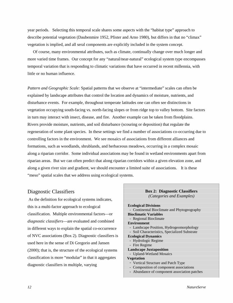
Diagnostic Classifiers As the definition for ecological systems indicates,
this is a multi-factor approach to ecological
classification. Multiple environmental factors—or
diagnostic classifiers—are evaluated and combined
in different ways to explain the spatial co-occurrence
of NVC associations (Box 2). Diagnostic classifiers is
used here in the sense of Di Gregorio and Jansen
(2000); that is, the structure of the ecological systems
classification is more “modular” in that it aggregates
diagnostic classifiers in multiple, varying
Box 2: Diagnostic Classifiers
(Categories and Examples) Ecological Divisions - Continental Bioclimate and Phytogeography
Bioclimatic Variables - Regional Bioclimate
Environment - Landscape Position, Hydrogeomorphology - Soil Characteristics, Specialized Substrate
Ecological Dynamics - Hydrologic Regime - Fire Regime
Landscape Juxtaposition - Upland-Wetland Mosaics Vegetation � ���Vertical Structure and Patch Type� - Composition of component associations - Abundance of component association patches

Ecological Systems of the United States 13
combinations. Instead of a specific hierarchy, we present a single set of ecological system types. This is
in contrast to, for example, the framework and approach of the IVC. The nested IVC hierarchy groups
associations into alliances based on common dominant or diagnostic species in the upper-most canopy.
This provides more of a taxonomic aggregation with no presumption that associations within the alliance
co-occur in a given landscape. The ecological system unit links IVC associations using multiple factors
that help to explain why they tend to be found together in a given landscape. Therefore, ecological
systems tend to be better “grounded” as ecological units than most IVC alliances and are more readily
identified, mapped, and understood as practical ecological units. Diagnostic classifiers include a wide
variety of factors representing bioclimate, biogeographic history, physiography, landform, physical and
chemical substrates, dynamic processes, landscape juxtaposition, and vegetation structure and
composition.
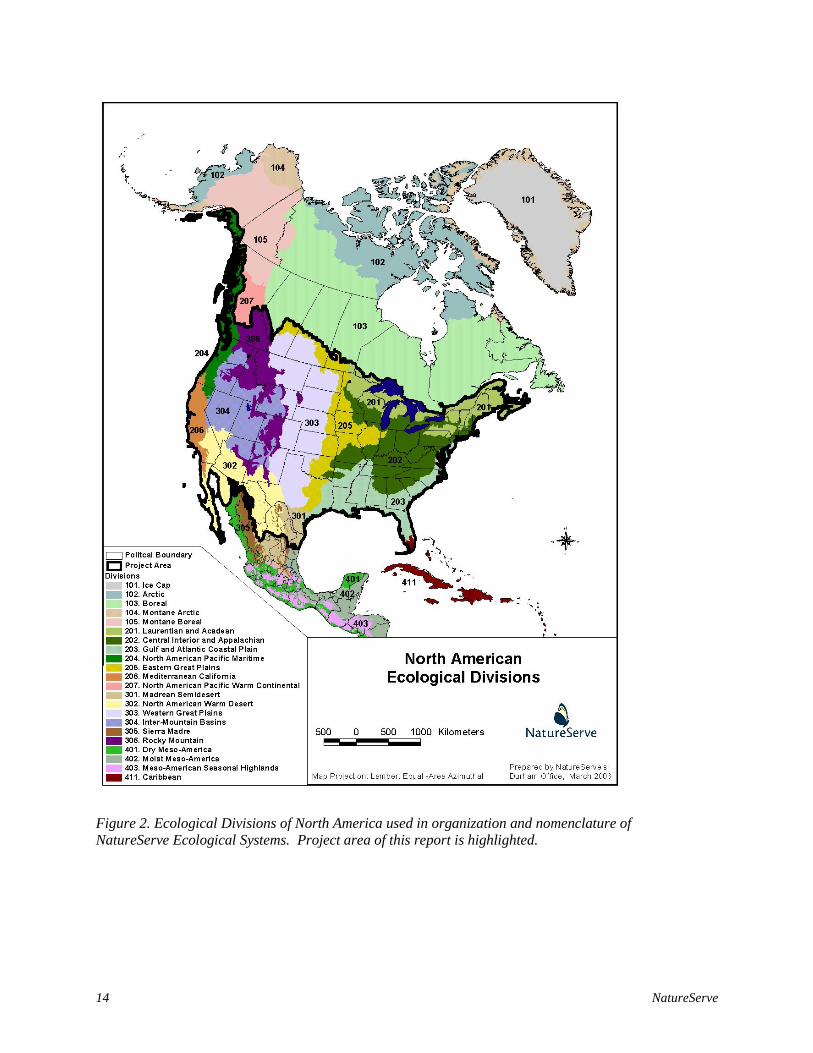
Biogeographic and Bioclimatic Classifiers. Ecological Divisions are sub-continental landscapes
reflecting both climate and biogeographic history, modified from Bailey (1995 and 1998) at the Division
scale (Figure 2). Continent-scaled climatic variation, reflecting variable humidity and seasonality (e.g.
Mediterranean vs. dry continental vs. humid oceanic) are reflected in these units, as are broad patterns in
phytogeography (e.g. Takhtajan 1986). The division lines were modified by using ecoregions established
by The Nature Conservancy (Groves et al. 2002) and World Wildlife Fund (Olson et al. 2001) throughout
the Western Hemisphere. These modified divisional units aid the development of system units because
regional patterns of climate, physiography, disturbance regimes, and biogeographic history are well
described by each Division. Thus, these divisions provide a starting point for thinking about the scale and
ecological characteristics of each ecological system. Examples of these Divisions include the Inter-
Mountain Basins, the North American Warm Desert, the Western Great Plains, the Eastern Great Plains,
the Laurentian and Acadian region, the Rocky Mountains, and the Atlantic and Gulf Coastal Plain. A
“Rocky Mountain” ecological system type is entirely or predominantly found (>80% of its total range)
within the Rocky Mountain Division. A “Southern Rocky Mountain” ecological system type is limited in
distribution to southern portions of the broader Rocky Mountain Division. In a few instances, ecological
systems remain very similar across two or more Ecological Divisions. In these instances, the Domain
scale of Bailey (1998) was used to name and characterize the distribution of types; e.g. the “North
American Arid West Emergent Marsh” spans the North American Dry Domain.
14 NatureServe
Figure 2. Ecological Divisions of North America used in organization and nomenclature of NatureServe Ecological Systems. Project area of this report is highlighted.
Ecological Systems of the United States 15
Subregional bioclimatic factors are also useful for classification purposes, especially where relatively
abrupt elevation-based gradients exist, or where maritime climate has a strong influence on vegetation.
We integrated global bioclimatic categories of Rivas-Martinez (1997) to characterize subregional climatic
classifiers. These include relative temperature, moisture, and seasonality. They may be applied globally,
so they aid in describing life zone concepts (e.g. ‘maritime,’ ‘lowland,’ ‘montane,’ ‘subalpine,’ ‘alpine’)
in appropriate context from arctic through tropical latitudes.
Environment: Within the context of biogeographic and bioclimatic factors, ecological composition,
structure and function in upland and wetland systems is strongly influenced by local physiography,
landform, and surface substrate. Some environmental variables are described through existing, standard
classifications and serve as excellent diagnostic classifiers for ecological systems. For example, soil
moisture characteristics have been well described by the Natural Resource Conservation Service (NRCS
1998). Practical hydrogeomorphic classes are established for describing all wetland circumstances
(Brinson 1993). Other factors such as landforms or specialized soil chemistry may be defined in standard
ways to allow for their consistent application as diagnostic classifiers.
Ecological Dynamics. Many dynamic processes are sufficiently understood to serve as diagnostic
classifiers in ecosystem classification. In many instances, a characteristic disturbance regime may
provide the single driving factor that distinguishes system types. For example, composition and structure
of many similar woodland and forest systems are distinguishable based on the frequency, intensity,
periodicity, and patch characteristics of wildfire (Barnes et al. 1998). Many wetland systems are
distinguishable based on the hydroperiod, as well as water flow rate, and direction (Brinson 1993;
Cowardin 1979). When characterized in standard form (e.g. Frost 1998), these and other dynamic
processes can be used in a multi-factor classification.
Landscape Juxtaposition. Local-scale climatic regime, physiography, substrate, and dynamic processes
can often result in recurring mosaics. For example, large rivers often support recurring patterns of levee,
floodplain, and back swamps, all resulting from seasonal hydrodynamics that continually scour and
deposit sediment. Many depressional wetlands or lakeshores have predictable vegetation zonation driven
by water level fluctuation. The recurrent juxtaposition of recognizable vegetation communities provides a
useful and important criterion for multi-factor classification.
Vegetation Structure, Composition, and Abundance: As is well recognized in vegetation classification,
both the physiognomy and composition of vegetation suggests much about ecosystem composition,
16 NatureServe
structure, and function. However, the relative significance of vegetation physiognomy may vary among
different ecosystems, especially at local scales. For example, many upland systems support vegetation of
distinct physiognomy in response to fire frequency and soil moisture regimes. In general, physiognomic
distinctions such as “forest and woodland,” “shrubland” “savanna,” “shrub steppe,” “grassland, “ and
“sparsely vegetated” are useful distinctions in upland environments. On the other hand, needleleaf or
broadleaf tree species that are either evergreen or deciduous may co-occur in various combinations due
more to variable responses to natural disturbance regimes or human activities than to current
environmental conditions. Many wetland systems could support herbaceous vegetation, shrubland, and
forest structures in the same location, again, based on the particular strategies of the species involved and
local site history.
Therefore, while recognizable differences in vegetation physiognomy may initially suggest
distinctions among ecosystem types, knowledge of vegetation composition should be relied upon more
heavily to indicate significant distinctions. As in vegetation classification, we recognize beta diversity, or
the turnover of species composition through space, as a primary means of differentiating ecosystem types.
The task of classification is to recognize where that turnover is relatively abrupt, and to explain why that
abrupt change occurs on the ground.
Standarized vegetation classifications, especially at the local scale described by the NVC association
concept, provide a useful tool for qualitative evaluation of vegetation similarity among ecological
systems. In locations where NVC associations are well developed, they serve as a useful summary of
quantitative data on the physiognomy and floristics of vegetation across the United States. For example,
two apparently similar forest ecosystems could be characterized in terms of the NVC associations they
support. We can assess the relative similarity of the two systems by comparing the association lists. Of
course, detailed and comprehensive association-scale classification is not always available, especially in
subtropical and tropical regions. In these instances, qualitative description and evaluation of non-standard
classification units is often sufficient for initial characterization of vegetation physiognomy and
composition among ecological systems.
While beta diversity is a primary consideration, the relative abundance of vegetation can also be an
important consideration. For example, riparian and floodplain systems may share many plant species, due
to their adaptation for dispersal along a seasonally flowing river. However, there may be substantial
differences in the relative abundance of vegetation between, for example, riparian systems with small,
flash-flood stream dynamics and a large, well-developed river floodplain many kilometers downstream.
Measurement of both vegetation patterns and environmental factors that support them are needed to
adequately address this facet of ecological classification.

Ecological Systems of the United States 17
Methods of Classification Development Ideally, ecological classification proceeds through several phases in a continual process of refinement.
These phases could include: 1) literature review and synthesis of current knowledge; 2) formulating an
initial hypothesis describing each type, that supports; 3) establishing a field sampling design; 4) gathering
of field data; 5) data analysis and interpretation; 6) description of types; 7) establishing dichotomous keys
to classification units; 8) mapping of classification units; and 9) refinement of classification, establishing
relative priorities for new data collection. Our approach is qualitative and rule-based, focusing on steps 1
and 2 above. We used existing information from other classifications as much as possible. In particular,
we utilized the existing ecoregional frameworks provided by ECOMAP (USDA Forest Service 1999),
particularly at the division level, to organize the process of defining systems. We relied on available
interpretations of vegetation and ecosystem patterns across the study area. And we reviewed associations
of the IVC/NVC in order to help define the limits of systems. Thus our approach draws extensively on
the existing literature available to us as well as on the extensive field experience of the contributors.
We divided NatureServe and natural heritage program ecologists into teams, based on Ecological
Divisions (Figure 2). Each team worked on developing systems within their division, noting those
systems whose range might extend outside the division. After all systems were described, we conducted
an overall review of all systems for eastern North America and western North America to ensure
consistency of concepts. In recent years we also conducted a number of tests of our systems approach
(e.g. Marshall et al. 2000, Moore et al. 2001, Hall et al. 2001, Nachlinger et al. 2001, Neely et al. 2001,
Menard and Lauver. 2002, Tuhy et al. 2002, Comer et al. 2002). In particular, we tested how well a
systems approach could facilitate mapping of ecological patterns at intermediate scales across the
landscape. These tests have led to the rule sets and protocols presented here.
Classification Structure The structure of the ecological systems classification could be described as “modular” in that it
aggregates diagnostic classifiers in multiple, varying combinations. This approach gives us maximum
flexibility in the definition of multi-factor units. In addition, we explicitly link our units to two existing
hierarchies 1) the vegetation hierarchy of the NVC, which provides a set of units from fine-scaled floristic
units to coarse-scaled formation units, and 2) the landscape ecosystem hierarchy of ECOMAP (Bailey
1995, USDA Forest Service 1999), particularly the levels from division down to subsection (see Box 1).
For the vegetation hierarchy we emphasize the linkage to association units, and for the landscape
hierarchy, we emphasize the Division level. Through database queries, we have also made it possible to

18 NatureServe
link units to the broad-scale map categories used for the National Land Cover Data (Forest, Shrubland,
Herbaceous, Woody Wetland, Herbaceous Wetland, Sparse or “barren” etc.).
However, some type of hierarchy for ecological system units may be advantageous. With
approximately 600 upland and wetland system types across the lower 48 United States, a hierarchy would
at least improve the organization of the units. But, more importantly, a hierarchy may also allow us to
further interpret the ecological patterns over a range of intermediate scales. Hierarchical arrangements of
biotopes or habitats in Europe (such as by EUNIS) may provide some guidance on establishing a
hierarchy of ecological systems presented here.
Development of Diagnostic Criteria and Descriptions Diagramming factors. Multiple diagnostic criteria may be arranged to allow for a visual expression of the
combinations that define each ecological system unit. Figure 3 depicts a subset of ecological system
types that are found in the Laurentian – Acadian Division. The major break between “upland” and
“wetland” was used as the initial stratifier. Matrix scale physiognomic breaks between “forested” vs.
“non-forested were then introduced. Within these classifiers, the primary disturbance regime, topography,
climate, and soils were used to further distinguish systems. These finer-scale classifiers set up constraints
on the type of floristic patterns that are associated with the systems. This type of diagramming visually
displays the logic of how major diagnostic classifiers are organized in developing systems. Subsequent
description and qualitative analysis allow these initial assumptions to be tested, then built upon.
Qualitative description. Each type is described in a database that includes a summary of known
distribution, environmental setting, vegetation structure and composition, and dynamic processes. A
separate portion of the database allows any combination of diagnostic classifiers to be attributed. This
permits subsequent sorts and further evaluation of types using any combination of diagnostic classifiers
(e.g. all riparian systems, all subalpine systems, all systems found in the Colorado Plateau, etc.).
Attribution of Plant Community Types. NVC associations are used to further describe each unit wherever
possible. Vegetation classification units in common usage in both California (Sawyer and Keeler-Wolf
1995) as well as in Alaska (Viereck et al. 1992) were also used when the NVC was incomplete in those
areas. Documented associations/communities are listed when there is evidence that they are found in
conditions described by the diagnostic criteria. Any occurrence of a given ecological system will have
some, but not necessarily all, of the listed communities.

E
colo
gica
l Sys
tem
s of
the
Uni
ted
Stat
es
19
������
�����!����
����
���
����"��#�����
����
�����������$����"�!����#�����������%�
�����������&��
'����������
���(&����!����
����������)������������*�������&������������
+����#��,�$!���������'&�������!��(&���%�
����������)����������*�������&��������
�������#��
����������-�������&�,�#�
�����������������
�������
����������
.���'�����
.���'�����
������
������
����������
/��������������
��
������'�����
��-��"��������
!����
���������
���#���������
��,���0�
���������
����#���
�������
�������
����
!��������
� � �
��������
��������������
����� �����
�����������
����������
����� �����
������
�����������
�����������
������
�����������
�����������
�����
�
��������
������������
�������� �
��������
������
�
��������
��������
�������
���������
������
�
��������
��������
������������
��������
������
�
��������
�������
����������
���������
������
�
������
����������
����
�����
� �����
���#��������
�������������!��������
��������
$�����%�
�������
��������$!���%�
��,����
���!�����
/�1��#�����
������2���
�&'������
!����
����������
���!!�-���&��
/�1���&������
�#��
������
�������
�&'������
�����
���&�
��&�������
����&��
�����
���&�
��&����
�������&��
������
��������
�������
����������������
������
�
��������
�!�������
�������������
������
�
��������
���������������
"��##�$�%����
�
��������
��������
"��������"��##�$�
%����
�
��������
���������������
������������
�
��������
��������
"��������
������������
�
&����������
��'��
�
�������� �
�����
���������
������"�����
�
Fig
ure
3. S
ampl
e de
cisi
on m
atri
x fo
r cl
assi
fica
tion
of s
elec
ted
ecol
ogic
al s
yste
ms
foun
d in
the
Lau
rent
ian-
Aca
dian
Eco
logi
cal D
ivis
ion.

20 NatureServe
Also, since associations/communities are principally used as descriptors of system units, some could
be predicted to occur within more than one ecological system type.
Pattern Type Review of broad scale ecological pattern for a given region should result in an initial suite of
ecological system types that could fall into one of four spatial categories (“matrix, large patch, small
patch, linear”) (Anderson et al 1999, Poiani et al 2000; see Table 1). For example, matrix-forming
forests, shrublands, and/or grasslands may dominate uplands for a given regional landscape.
Knowledge of environmental variation, dynamic processes, and resulting compositional variations
can be used to qualitatively characterize system types that typically occur in patches ranging from
2,000 on up to 10,000s of hectares. Both large patch and small patch systems tend to appear nested
within matrix system types, while linear system types occur along riverine corridors, coastal areas,
and major physiographic breaks (e.g., escarpments or cliff faces). Analysis of local-scale patterns
nested within a region’s natural matrix clarifies the diversity of potential patch and linear system
types.
We use these four categories of spatial scale in order to avoid subsuming distinctive biotic and
abiotic factors into larger systems, where those factors are clearly different from the matrix or large
patch systems. But, the smaller the potential system, the more distinctive these factors needed to be
to justify recognizing it as distinct. Thus, e.g., seepage fens are distinguished from their surrounding
matrix forests or large-patch floodplain systems because of the distinctive biotic and abiotic factors
present, whereas ox-bows or backwater swamps are not distinguished within a floodplain system.
The concepts of both “linear” and “small patch” types typically result in the definition of units
that clearly fall into either category. The same is not always true with “large patch” vs. “matrix”
types. There are circumstances where an ecological system forms the matrix within one part of its
range, but then occurs as a “large patch” type in another part of its range. This likely results in
differing dynamics of climate and related disturbance processes – and interactions with other systems
– that vary in ways unique to each system type. For example, a savanna system may form the matrix
of one ecoregion where landscape-scale fire regimes have historically been supported by regional
climate. An adjacent, more humid ecoregion might support the same type of savanna system, but
occuring as patches within a matrix of forests. Importantly, we have established as a classification
rule that this type of change in spatial character – between “large patch” and “matrix” categories
across the range of a type does not force the distinction between two system types. The
environmental and disturbance dynamics that result in that variation can be described and addressed
for conservation purposes without defining a distinct type.

Ecological Systems of the United States 21
Table 1. Categories for patch types used to describe ecological systems
Patch Type Definition Matrix Ecological Systems that form extensive and contiguous cover, occur on the most
extensive landforms, and typically have wide ecological tolerances. Disturbance patches typically occupy a relatively small percentage (e.g. <5%) of the total occurrence. In undisturbed conditions, typical occurrences range in size from 2,000 to 10,000s ha.
Large Patch Ecological Systems that form large areas of interrupted cover and typically have narrower ranges of ecological tolerances than matrix types. Individual disturbance events tend to occupy patches that can encompass a large proportion of the overall occurrence (e.g. >20%). Given common disturbance dynamics, these types may tend to shift somewhat in location within large landscapes over time spans of several hundred years. In undisturbed conditions, typical occurrences range from 50-2,000 ha.
Small patch Ecological Systems that form small, discrete areas of vegetation cover typically limited in distribution by localized environmental features. In undisturbed conditions, typical occurrences range from 1-50 ha.
Linear Ecological Systems that occur as linear strips. They are often ecotonal between terrestrial and aquatic ecosystems. In undisturbed conditions, typical occurrences range in linear distance from 0.5 to 100 km.
Nomenclature for Ecological Systems The nomenclature for the ecological systems classification includes three primary components that
communicate regional distribution (predominant Ecological Division), vegetation physiognomy and
composition, and/or environmental setting. The final name is a combination of these ecological
characteristics with consideration given to local usage and practicality.
Ecological Divisions: The Division-scaled units typically form part of each classification unit’s
name. For example, a “Rocky Mountain” ecological system unit is entirely or predominantly found
(>80% of its total range) within the Rocky Mountain Division, but could also occur in neighboring
Divisions. This nomenclatural standard is applicable to most ecological system units, except for
those types that span many several Divisions (e.g., some tidal or freshwater marsh systems), or that
are more localized (>80% of the range) within a subunit of the Division (e.g., Colorado Plateau,
within the Inter-Mountain Basins Division).
Vegetation Structure and Composition: Vegetation structure (e.g., Forest and Woodland, Grassland),
and vegetation composition (e.g. Pinyon-Juniper, mixed conifer) is commonly used in the name of a
system. In sparse to unvegetated types, reference to characteristic landforms (e.g., badland, cliff) may

22 NatureServe
substitute for vegetation structure and/or composition. It will typically come after Ecological
Division, but may come before or after Environment.
Environment: Environmental factors (e.g., xeric, flats, montane) can be used in conjunction with
Vegetation Structure and Composition or, on their own, to name system types. This will typically
come after Ecological Division, but may come before or after Vegetation Structure and Composition.
Examples:
Laurentian-Acadian Pine-Hemlock-Hardwood Forest
Cross Timbers Oak Forest and Woodland
Central Appalachian Limestone Glade and Woodland
Southern and Central Appalachian Cove Forest
North-Central Interior Shrub-Graminoid Alkaline Fen
Cross Timbers Oak Forest and Woodland
Western Great Plains Wooded Draw and Ravine
Rocky Mountain Foothill Grassland
Chihuahuan-Sonoran Desert Bottomland and Swale Grassland

Ecological Systems of the United States 23
Results
Number and Distribution of Systems This project identified and described 599 upland and wetland ecological systems within the
project area. They represent the full range of natural gradients, with some 381 types (63%) being
uplands, 183 types (31%) being wetland, and 35 types (6%) being complexes of uplands and
wetlands. Excluding upland/wetland complexes, some 322 types (54%) are predominantly forest,
woodland, and/or shrubland, and some 166 types (28%) are predominantly herbaceous, savanna, or
shrub steppe. Seventy-four systems (12%) are sparsely vegetated.
A geographic breakdown of ecological system types indicates some expected patterns. Using
continental Domain units as one frame of reference (Bailey 1998), within the project area, some 430
types are known to occur in the Humid Temperate Domain (all Pacific coast regions and nearly all of
the eastern United States). Another 246 types are attributed to the Dry Domain (from the western
Great Plains across the Intermountain West), and 21 units occur in the Humid Tropical Domain
(south Florida). Figure 4 indicates the numbers of ecological system units by Ecological Division.
The relatively large number of types found in the Gulf and Atlantic Coastal Plain and Central Interior
and Appalachian divisions is not unexpected. Each of these large and complex divisions has over 100
ecological system units attributed. Divisions that encompass most of the West, including the Rocky
Mountain Division, North American Pacific Maritime, Inter-Mountain Basins, and Mediterranean
California include between 60 and 90 types each. The Laurentian-Acadian, Eastern Great Plains,
Western Great Plains, and North American Warm Desert divisions each include between 31 and 60
types. Both the Madrean Semidesert and the Caribbean divisions include portions within the
coterminous United States, but data from remaining portions were not included in this project area.
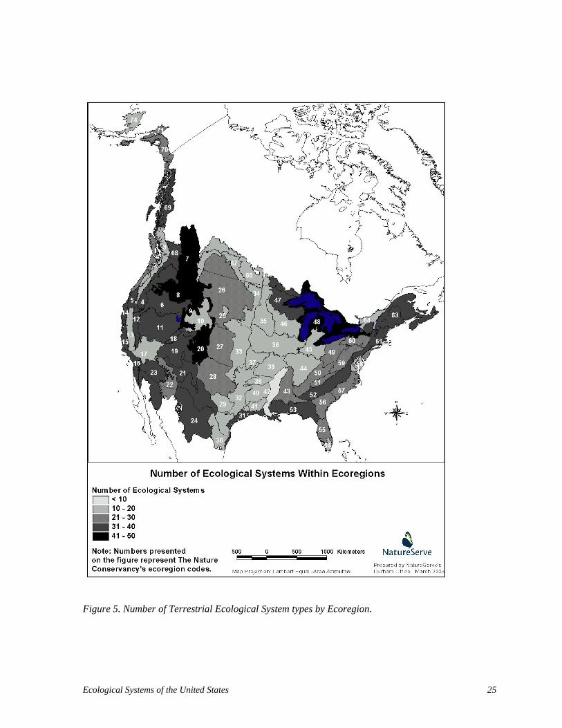
Figure 5 depicts numbers of ecological system units within each ecoregion currently used by The
Nature Conservancy within the project area. These range from highs of nearly 50 types in the Great
Lakes and several Rocky Mountain ecoregions to a low of fewer than 10 for the Mississippi River
Alluvial Plain. The mean number for ecoregions included in the project area was 25 types. This
obviously varies by size and complexity of the ecoregion.
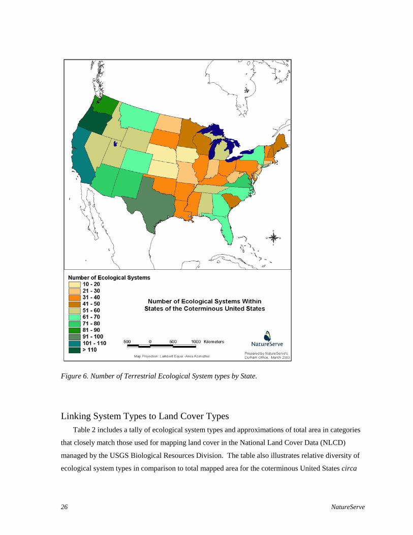
Figure 6 depicts the number of ecological system units for each state in the coterminous United
States. Again, numbers vary by size and ecological complexity of each state. Over 100 units are
attributed to Oregon and California. The states of Texas, Virginia, Washington, New Mexico and
Arizona include between 70 and 100 types each. Some 13 states, from Michigan to Florida include
between 51 and 70 types each. Another 17 states, from Minnesota to South Dakota include between

24 NatureServe
30 and 50 types. The remaining 11 states in the project area each have fewer than 30 types currently
attributed.
Figure 4. Number of Terrestrial Ecological System types by Ecological Division.
Ecological Systems of the United States 25
Figure 5. Number of Terrestrial Ecological System types by Ecoregion.
26 NatureServe
Figure 6. Number of Terrestrial Ecological System types by State.
Linking System Types to Land Cover Types Table 2 includes a tally of ecological system types and approximations of total area in categories
that closely match those used for mapping land cover in the National Land Cover Data (NLCD)
managed by the USGS Biological Resources Division. The table also illustrates relative diversity of
ecological system types in comparison to total mapped area for the coterminous United States circa

Ecological Systems of the United States 27
1992. In these terms, both herbaceous and woody wetland types, as well as sparely vegetated types
are relatively diverse, followed by forests, shrublands, and herbaceous types.
In the NLCD classification, the “Forest” class is a combination of the “Forest” and “Woodland”
Formation Classes in the National Vegetation Classification (NVC). Similarly, the NLCD
“Shrubland” class encompasses the “Shrubland” and “Dwarf-shrubland” Formation Class of the
NVC, and NLCD “Grasslands/Herbaceous” matches the “Herbaceous” Formation Class of the NVC.
The NLCD “Woody Herbaceous” class includes upland NVC Formation Groups of “Temperate or
subpolar grassland with a sparse tree layer” and “Temperate and subpolar grassland with a sparse
shrub layer.” This class is not comprehensively mapped in the NLCD. NLCD “Woody Wetlands”
encompasses some 80 wetland and saturated Forest, Woodland, and Shrubland Formations of the
NVC. Some 43 wetland and saturated Herbaceous NVC Formations make up the “Emergent/
Herbaceous Wetland” class of NLCD. The NLCD “Bare Rock” class closely matches the NVC
Sparse Vegetation Formation Class, but could also include areas classified in the Nonvascular
Formation class of the NVC.
Table 2. Breakdown of ecological system types in terms of prevailing vegetation physiognomy and
upland/wetland status, closely matching categories mapped in National Land Cover Data.
Prevailing Physiognomy and Environment (modified from NLCD 1992)
Number of Ecological
System Types
Percentage of Total Number of
Types
Area in Coterminous United States (circa 1992)
[ miles2 and %] Forest (Evergreen, Deciduous, Mixed)
152 25% 879,858 (29%)
Shrubland (Tall, Short, Dwarf) 71 12% 564,713 (19%) Woody Herbaceous 30 5% N/A Grasslands/Herbaceous 56 9% 479,074 (16%) Woody Wetlands 100 17% 85,412 (3%) Emergent/Herbaceous Wetlands 83 14% 37,982 (1%) Mixed Upland and Wetland 35 6% N/A Bare Rock (Sparsely Vegetated) 74 12% 42,640 (1%)
Data Management and Access
The classification information is stored in a MS-Access database (Systems2000.mdb). The
database includes descriptions of the approximately 600 systems types, their distribution by states and
ecoregions, the list of NVC associations that characterize them, and many literature references. It
also includes the diagnostic classifiers used to define the ecological systems. Small subsets of
systems from several TNC ecoregions also have Element Occurrence (EO) Specifications and EO
Rank Specifications stored in the database (see also Appendix 2). The database is available in both
Access 97 and Access 2000 versions, in both cases in read-only format. An accompanying manual in

28 NatureServe
MS-Word (Systems database manual.doc) documents its content, functionality, and reporting
capabilities.
During 2003, all of the US Terrestrial Ecological Systems and their accompanying data will be
converted into NatureServe’s central data management system, Biotics 4. Once the system types and
the data are stored in Biotics 4, the full data management, updating, and revision capabilities of that
will be available for the continuing development and refinement of system types. In addition, the
ecological systems will be served on-line via NatureServe’s public website (www.natureserve.org),
and NatureServe Explorer, an online searchable databases of species and ecological communities
(www.natureserve.org/explorer).

Ecological Systems of the United States 29
Applications
Applications to Conservation Assessment Conservation assessment occurs at varying spatial scales to serve the needs of various users.
Assessment at a regional scale is often necessary to evaluate status and trends in regional biodiversity.
Places are then identified that capture ecological and genetic variation across a broad range of
environmental gradients (Johnson et al. 1999). At these regional scales, planning efforts may identify
networks of places that, taken together, fully represent characteristic biological diversity. One might
then identify areas where more intensive natural resource development could take place in a
compatible fashion. That network of places is sometimes referred to as a “portfolio,” because a
variety of approaches may be used to conserve biological diversity over time through on-the-ground
actions. As knowledge expands, and the “market” for conservation changes, one can expect that new
places will gain importance, while other places may contribute less to conservation goals. Much like
a financial portfolio, a regional conservation portfolio is flexible and priority-based.
Assessments using ecoregions as a spatial planning framework have become increasingly common
in recent years, and standardized classifications of ecological systems can serve a central role.
Ecoregions are regional landscapes, or relatively large areas of land and water defined by similar
geology, landforms, climates and ecological processes. Further, ecoregions contain geographically
distinct assemblages of ecological systems that share a large majority of their communities, species,
dynamics, and environmental conditions, and function effectively as a framework for conservation at
global and continental scales (Bailey 1996, Olsen et al. 2001). In most instances, upland and wetland
ecological systems can be mapped comprehensively across ecoregions or any other regional planning
area. Therefore they aid in evaluating the status and trends of numerous ecological phenomena, from
trends in land conversion or wildlife habitats to creating repeatable metrics for landscape
fragmentation. Because ecological system units are defined to represent characteristic composition,
structure, and function at intermediate scales, conservation goals aimed at conserving ecological
systems should also capture ecological processes important to many, but not all, biological
communities and species.
An “element-based” approach to conservation assessment commonly establishes a suite of species,
communities, and ecological systems that provide the focus for representing biodiversity. An
additional suite of elements may also be included in the analysis to represent overall conservation
value (e.g., those identified under environmental regulations, open space, scenic or cultural values.).
The objective should be to select a limited set of elements that could serve as effective surrogates for
all (or nearly all) biological diversity. Through conservation of these elements across the planning

30 NatureServe
area, one seeks to efficiently secure the ecological environments and dynamic interactions that
support the vast majority of species. Occurrences of these elements, as well as the relative quality of
their occurrences, are used to characterize biodiversity value and identify specific locations for
conservation action.
To identify these elements effectively, one may use several sets of selection criteria. Typically one
should include elements from multiple levels of ecological organization, elements representing
varying degrees of rarity, vulnerability, and endemism (Appendix 3), and elements representing
multiple geographic scales of habitat/area requirement. The outline in Table 3 summarizes
recommended criteria to select elements. Elements of biological diversity – the ecological systems,
communities, species assemblages, and species — that meet at least one of the criteria in the outline
are therefore placed on the list of selected elements.
Table 3. Core Selection Criteria for Elements for Biodiversity Conservation _______________________________________________________________________ I. Ecological systems. A. All natural/semi-natural terrestrial ecological systems that are known to occur in the planning area. B. All natural/semi-natural aquatic ecological systems that are known to occur in the planning area. II. Ecological communities. A. Rare natural/semi-natural terrestrial plant associations globally ranked G1-G3 by the Natural
Heritage Network. B. Rare natural/semi-natural aquatic macrohabitats globally ranked G1-G3 (where available). C. Vulnerable species assemblages – e.g. areas where concentrations of migratory species occur. III. Species (including infraspecific taxa). A. Species globally ranked G1-G3; subspecies/varieties globally ranked T1-T3. B. Species (subspecies) globally ranked G4-G5 (T4-T5), that on the whole are “of concern” by virtue
of: 1. Experiencing significant decline across their range. 2. Are currently stable, but vulnerable to future declines, due for example to their broad
regional landscape requirements or to their concentration in particular areas during their migrations.
3. Are considered endemic to the planning area. 4. Having widely disjunct occurrences in the planning area.
5. Are considered to be “keystone” species. ______________________________________________________________________________ Using these selection criteria, three levels of biological or ecological organization: ecological
systems, communities, and species, are represented among selected elements. As these categories
indicate, this reflects a “coarse filter/fine filter” hypothesis – i.e. the conservation of multiple, high-
quality occurrences of all ecological systems will also support the majority of native biodiversity.
Since this “coarse filter” on its own would be unlikely to represent all biodiversity, especially those
that are rare and thus not reliably found within most examples of ecological systems, additional

Ecological Systems of the United States 31
elements, those that are imperiled or vulnerable, are also needed – the “fine filter.” Experience
suggests that this is the most efficient and effective approach to capturing biodiversity in a network of
reserves (e.g. Jenkins 1976, 1985; Noss and Cooperider 1994, Haufler et al. 1996, Groves et al. 2002,
Kintsch and Urban 2002). The coarse filter/fine filter approach also reduces complexity and cost
associated with strict species-based approaches (e.g. Scott et al 1987, Beissinger and Westphal 1998;
Willis and Whittaker 2002) while allowing sufficient flexibility to integrate new approaches as
technical hurdles are overcome (e.g. Fleishman et al. 2001, Carroll et al. 2001, Scott et al. 2002).
Careful element selection therefore provides appropriate focus for efforts to map and evaluate
element occurrences, then establish specific conservation goals and objectives.
Applications to Element Occurrence Inventory and Mapping
Element Occurrences: Information on status and trends of ecosystems is critical for evaluation,
conservation, and management of natural resources. NatureServe and natural heritage scientists
develop detailed information about the location and viability or integrity of biodiversity elements and
about the sites that are important for their persistence or survival. They help reduce negative impacts
on biodiversity by providing this information in ways that facilitate awareness of the key impacts that
various development projects may have (Stein and Davis 2000). Here we discuss the first key part of
the mission as it relates to ecological systems - identifying the systems on the ground and developing
detailed information on their locations or occurrences (“element occurrence specifications”). In the
next section (Applications to Management and Monitoring), we introduce the issue of assessing the
ecological integrity of these occurrences (see also Appendix 2).
Elements, then are the units of biodiversity, whether species, communities, or systems. Element
occurrences are geographic locations of those elements on the ground. Specifically, NatureServe
standards (NatureServe 2002) state that:
An element occurrences (EO) is an area of land and/or water in which a species,
natural community, or ecological system is, or was, present. An EO should have
practical conservation value for the Element…. For community Elements, the EO may
represent a stand or patch of a natural community, or a cluster of stands or patches of a
natural community. For system elements, the EO may represent a cluster of stands from
different communities that are part of the system.
Element occurrences are the principal source of information about the distribution of the elements.
The occurrences are typically mapped, often at the scale of 1:24,000, but scale can vary depending on
the application.
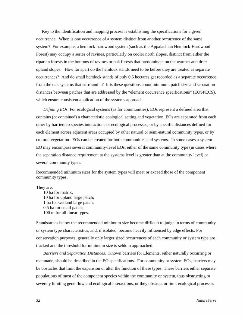
32 NatureServe
Key to the identification and mapping process is establishing the specifications for a given
occurrence. When is one occurrence of a system distinct from another occurrence of the same
system? For example, a hemlock-hardwood system (such as the Appalachian Hemlock-Hardwood
Forest) may occupy a series of ravines, particularly on cooler north slopes, distinct from either the
riparian forests in the bottoms of ravines or oak forests that predominate on the warmer and drier
upland slopes. How far apart do the hemlock stands need to be before they are treated as separate
occurrences? And do small hemlock stands of only 0.5 hectares get recorded as a separate occurrence
from the oak systems that surround it? It is these questions about minimum patch size and separation
distances between patches that are addressed by the “element occurrence specifications” (EOSPECS),
which ensure consistent application of the systems approach.
Defining EOs. For ecological systems (as for communities), EOs represent a defined area that
contains (or contained) a characteristic ecological setting and vegetation. EOs are separated from each
other by barriers to species interactions or ecological processes, or by specific distances defined for
each element across adjacent areas occupied by other natural or semi-natural community types, or by
cultural vegetation. EOs can be created for both communities and systems. In some cases a system
EO may encompass several community-level EOs, either of the same community type (in cases where
the separation distance requirement at the systems level is greater than at the community level) or
several community types.
Recommended minimum sizes for the system types will meet or exceed those of the component community types. They are: 10 ha for matrix, 10 ha for upland large patch; 1 ha for wetland large patch; 0.5 ha for small patch; 100 m for all linear types. Stands/areas below the recommended minimum size become difficult to judge in terms of community
or system type characteristics, and, if isolated, become heavily influenced by edge effects. For
conservation purposes, generally only larger sized occurrences of each community or system type are
tracked and the threshold for minimum size is seldom approached.
Barriers and Separation Distances. Known barriers for Elements, either naturally occurring or
manmade, should be described in the EO specifications. For community or system EOs, barriers may
be obstacles that limit the expansion or alter the function of these types. These barriers either separate
populations of most of the component species within the community or system, thus obstructing or
severely limiting gene flow and ecological interactions, or they obstruct or limit ecological processes

Ecological Systems of the United States 33
that these species depend on. Barriers may be common for many wetland communities or systems,
but are typically less common for many upland terrestrial communities or systems.
In addition to barriers that totally, or almost completely, prevent ecological processes and species
interactions, there may be habitats between two stands of an element that partially restrict species
interactions or ecological processes. Unlike barriers, their effect depends on the kind and extent of
this intervening habitat. This leads to the issue of separation distance. Assigning values for
separation distances between two stands promotes consistency in the manner in which EOs are
defined and mapped. Smaller separation distances are used when the intervening habitat is highly
restrictive to the ecological processes or species interactions the element depends, and greater
distances are used when these habitats are less prohibitive to ecological processes or species
interactions.
We use two broad categories of intervening habitats to define separation distances, namely –
natural/semi-natural vegetation or cultural vegetation. Generally speaking, intervening natural and
semi-natural vegetation will have less of an ecological effect between two stands of an EO than
intervening cultural vegetation. Thus rather simplistically, we suggest that different separation
distances be specified for these two kinds of situations. Typically, a shorter separation distance is
specified when the intervening habitat is cultural vegetation than when it is natural/semi-natural.
Minimum values for separation distances have been recommended to ensure that EOs are not
separated by unreasonably small distances, which would lead to the identification of unnecessarily
splintered stands as potential targets for conservation planning or action. For communities or
systems, the minimum separation distance for intervening areas of different natural or semi-natural
communities is set at 1 km or greater, and for intervening areas of cultural vegetation, the distance is
set at 0.5 km or greater (Table 4). These separation distances may, of course, be much larger. For
communities or systems found primarily in mountainous regions, where habitat tends to be less
fragmented, separation distances may be 5 km or more. A few elements may require separation
distances that are less than the established minimum; in such cases, these distances should be justified
in the EO specifications. Again, more detailed explanation and examples of these issues are found in
Appendix 2.
These separation distances may be further refined by considering the kind of natural/semi-natural
or cultural vegetation present. Intervening natural and semi-natural areas with similar kinds of habitat
characteristics to the stands of a community or system under consideration will have less of an effect
on community or system processes than those with very different kinds of characteristics. For
example, bog stands separated by intervening areas of upland jack pine on bedrock could be more

34 NatureServe
readily treated as distinct EOs than bogs separated by areas of black spruce swamp. However, at this
time, no specific guidelines are suggested for these situations.
Table 4. Recommended Minimum Separation Distances for Communities and Ecological Systems
Type of Separation Minimum Separation Distance
Barrier qualitatively defined
cultural vegetation ≥ 0.5 km
different natural or semi-natural communities or systems
≥ 1 km
Applications to Comprehensive Mapping Comprehensive mapping of terrestrial ecological systems draws heavily on the experience of
mapping vegetation using remotely sensed imagery and ancillary data (e.g., the USGS-BRD/NPS
Vegetation Mapping Program standards as outlined by Grossman et al. 1994; Faber-Langendoen et
al. 2002). That methodology recognizes that vegetation forms one of the most readily observable
natural features of the landscape. It provides an important measure of the current condition of natural
systems and can serve as a cost-effective monitoring tool for ongoing management of those systems.
Vegetation mapping is the process of integrating multiple sets of information. It often involves
interpreting signatures from vegetation from remotely sensed data – sometimes integrating ancillary
spatial data - then assigning each signature to a map unit. In order to ensure that each mapper bases
his or her interpretation of those signatures on the same ecological perspective, a consistent
classification is needed.
Given the inherent difficulties in achieving a consistent classification scheme, it may appear that
classification should really be the end result of mapping; that is, the vegetation mapper is free to
explore the vegetation patterns as they appear on the local landscape, and choose those features that
are most relevant to the species combinations and environmental factors on hand (a posteriori
classification). Indeed, Kuchler (1988) argued that this approach has much to recommend it. But
Kuchler also pointed out that such a posteriori classifications have a major drawback – they are best
applicable only in the mapped area or, at best, only short distances beyond the borders of the area.
Since the scope of both the National Vegetation Classification and the NatureServe Ecological
Systems Classification is national - indeed hemispheric - basing the mapping on these classifications

Ecological Systems of the United States 35
should allow any map produced to be compared to other areas throughout the country in an integrated
and consistent manner. It is for that reason, for example, that federal agencies such as the USGS Gap
Analysis Program and the National Park Service chose in the mid-1990s to work with an a priori
classification, the NVC, seeking to balance the needs of mapping local vegetation patterns with the
overall need to achieve consistency across the nation.
Mapping Issues with the NVC: The stated intention of the Gap Analysis Program for land cover
mapping has been to depict vegetation matching the scale and concept of the vegetation Alliance, as
described in the NVC. However, not all vegetation types are equally mappable at a given geographic
scale. GAP efforts to map vegetation on a statewide scale have had difficulty achieving desired levels
of mapping accuracy for map units reflecting all vegetation alliances. This is due to the reality that
not all Alliances occur in large and distinctive patches that are easily depicted with satellite imagery.
As examples, many wetlands and herbaceous uplands may include several Alliances co-mingled
within a few hectares. As one works at scales of multiple states, the problem of consistent Alliance-
scale mapping increases. Figure 7 depicts a combined coverage from five central United States (CO,
KS, NE, SD, and WY). While Alliance-level units were mapped in each state, the success at
achieving this scale varied significantly. In addition, where some states were able to achieve Alliance
scale units, their neighboring states that also include the same vegetation types may not have been as
successful. As a result, any regional coverage will tend to include fewer Alliance-scale units depicted
consistently across the map area than for any given state or subregion. In this instance, only 17
Alliances were mapped consistently across this area; just a small subset of those that are known to
exist on the ground.
So while many Alliances can be mapped by using both remotely sensed imagery and an
understanding of the ecological factors that help define them (e.g., elevation, soil type, aspect), some
Alliances remain indistinguishable using remotely sensed imagery. The reasons for this vary but
common examples are that species that differentiate similar Alliances occur beneath a dense canopy of
trees or shrubs, that differential species had very similar signatures when the imagery was acquired, or
that the scale of the Alliances is below the standard minimum mapping unit.
To maintain the a priori classification, the mapping team may consider using higher levels of the
NVC hierarchy as map units. NVC units at “middle-levels” of the hierarchy, such as Formation, are
driven primarily by vegetation physionomy, rather than considerations of spatial scales and ecological
variables. Whereas the NVC Association unit is typically mappable at scales of around 1:24,000 or
larger and often corresponds to ecological factors at that scale, it is more difficult to identify typical

36 NatureServe
Figure 7. Alliance-scale units mapped comprehensively across CO, KS, NE, SD, and WY (from Comer et al. 2003).
spatial scales and ecological patterns for the mid-level units. So the higher levels of the NVC hierarchy
do not necessarily provide suitable classification units for mapping at “coarser” (smaller) scales. Of
particular note for applying the NVC to mapping, three aspects are worthy of further exploration: 1)
the practical “constraints” imposed by the physiognomic hierarchy on classification units, 2) the
variable, and sometime wide, ecological “distance” between Formation, Alliance, and Association
levels of the NVC, and 3) potential difficulties for mapping some environmental attributes of the
NVC, regardless of minimum map units size.
1. Because the NVC is a strictly nested hierarchy, classification attributes from higher levels are
carried over to units further down. So for example, physiognomic distinctions (e.g. forest vs.
woodland, evergreen vs. deciduous, needleleaf vs. broadleaf) that enter in the classification at
the Class, Subclass, Formation Group, and Formation levels are carried over directly to nested
Alliance and Association units. Vegetation types that differ in any one physiognomic attribute

Ecological Systems of the United States 37
(e.g. forest vs. woodland) form distinct Alliances and Associations, although they may co-
mingle on a given landscape.
2. For some types of vegetation, the differences between Formation, Alliance, and Association
scales are quite large. For example, a “short bunch temperate or sub-polar grassland
Formation” or “lowland or submontane cold deciduous forest Formation” unit likely
encompasses hundreds of alliances and thousands of associations around the globe. On the
other hand, the “caespitose needle-leaved or microphyllous evergreen dwarf shrubland
Formation” or the “creeping or matted drought-deciduous dwarf shrubland Formation” likely
include relatively few alliances and associations around the globe. Similarly, some widely
distributed Alliances (e.g. Pinus ponderosa Woodland Alliance) include much variability, as
expressed by over 50 Associations, while other alliances may include only one or just a few
associations. This variability among different NVC units can make systematic “aggregations”
of map units up from Associations, to Alliances and Formations awkward and often
undesirable.
3. Although the NVC hierarchy is primarily based on vegetation, it also uses climatic, topographic
and other criteria as a practical tool for dividing the vegetation units. Several environmental
attributes enter the NVC hierarchy at the Formation level. Among these are hydrologic
modifiers (e.g. temporarily flooded, seasonally flooded, semi-permanently flooded, etc.) that
require very detailed, if not multi-temporal, data to accurately apply. So simply “aggregating
up” from finer scales to what is often viewed as a rather “coarse” Formation scale still may not
solve the mapping problem.
To these considerations we must add the reality of incomplete development for the NVC.
Remarkable progress on the classification has been made in the years since 1994. Large portions of
some 5,000 Associations have been described; however, parts of the landscape remain inadequately
accounted for in the NVC. It is safe to say that we will be coping with our ignorance for some time to
come, so the ability to work flexibly at multiple, systematically defined levels of thematic resolution
remains highly desirable.
The NVC, therefore, provides a hierarchical classification structure that allows for varying levels
of floristic and physiognomic detail, but depending on the circumstances, mapping protocols can
easily permit designations of mapping mosaics that are “ad-hoc” or overly driven by observed
patterns in available imagery. This, in part, defeats the purpose of an a priori classification that is
intended to guide the mapping process. One approach to address this situation is to develop
classifications above the NVC Association scale that circumvent some of the mapping-related

38 NatureServe
problems inherent in the NVC hierarchy, but still provide units that are practical and useful for
management and conservation. Some of the issues identified above could be resolved by revising the
NVC hierarchy itself—indeed, the FGDC hierarchy revisions working group proposes to undertake
such revisions in the near future. Others, however, require a different approach that focuses on the
ecological and spatial relations among the types, rather than just the vegetation relations. The
ecological systems classification is intended in part to address this situation.
Ecological Systems provide “meso-scaled” units as a basis for analyzing vegetation patterns,
habitat usage by animals and plants, and systems-level comparisons across multiple jurisdictions.
They also provide useful, systematically defined, groupings of NVC Alliances and Associations,
forming the basis of map units where Alliance and/or Association level mapping is impractical.
Figure 8 depicts some 63 terrestrial ecological system units mapped across the same five
Figure 8. Terrestrial ecological system-scale units mapped comprehensively across CO, KS, NE, SD, and WY (from Comer et al. 2003).
states shown in Figure 7. The same vegetation coverages used for the alliance-level map in Figure 7
were used again, but, in addition, biophysical variables such as elevation, landform, surface geology,

Ecological Systems of the United States 39
soils, and hydrography were also brought in. These variables were combined with the concept
statements of each ecological system type to create a map of terrestrial ecological systems (Comer et
al. 2003). Not all of the 90 terrestrial ecological system units thought to occur in this five-state
region were depicted in this map with existing data. Those not depicted tend to occur as very small
patches (e.g. montane fens), or are known to occur primarily in adjacent states, but likely have limited
occurrence within this map project area. However, future efforts should have considerably more
success if these a priori ecological system units are the mapping objective.
Many of the same mapping issues from regional efforts extend to more localized projects, even
those where low-elevation aerial photo interpretation is the principal remotely sensed-data. An
example from Zion National Park illustrates a common circumstance with more local-scale mapping
efforts (Cogan et al. 2002). Here, as with all National Park Service vegetation mapping, the stated a
priori classification and mapping objective is the NVC Association.
Zion NP is a relatively large park (593 km2 or 229 mi2). Major regional floras influence the
vegetation, with Mojavean elements in the southwestern portion, Great Basin floristics in the western
portion, and influences of the Colorado Plateau and southwestern Utah flora in the eastern and
northern portion. Vegetation diversity is high because the elevation gradient extends for nearly a mile
(1125-2600 m, 3680-8726 ft) and the landscape is complex. Field-based sampling and classification
work in Zion NP resulted in 97 described NVC Associations. Of the 42 natural/near-natural
vegetation map units, 20 match the scale and concept of NVC Association, 14 match the NVC
Alliance, four match NatureServe Terrestrial Ecological System units, and four would represent a
combination of Ecological System units. The 42 original map units correspond to 20 Ecological
Systems, providing a park-wide perspective on the Ecological System units found within the park
(Figure 8). Figure 8 provides a park-wide perspective on the Ecological System units found within
the park and the one-mile buffer, along with aquatic and land use features. Two system types, Great
Basin Pinyon-Juniper Woodland and Colorado Plateau Pinyon-Juniper Woodland, were not
distinguished in the fine-scale map units, so they are represented as one combined unit. Given our
knowledge of the elevation ranges that distinguish these two pinyon-juniper units, they could be
feasibly mapped as separate units.
The most prevalent systems across this park landscape include these two types of Pinyon –
Juniper Woodlands, Rocky Mountain Gambel Oak Mixed – Montane Shrublands, Colorado Plateau
Mixed Bedrock Canyon and Tableland, Rocky Mountain Ponderosa Pine Woodland, and Rocky
Mountains Bigtooth Maple Ravine Woodland.
Mapping efforts at Zion NP were ongoing at the time of this publication, but existing data were
sufficient for a preliminary accuracy assessment. Raw accuracy scores for each fine-scale map unit

40 NatureServe
yielded a total accuracy of 489 correct points out of 781 samples, or 63% accuracy. A comparable
assessment for the map of ecological system units yielded 609 correct points out of 800 samples, or
76% accuracy (Comer et al. 2002).
Figure 9. Terrestrial ecological systems of Zion National Park and environs (scale ~ 1: 200,000) (from Comer et al. 2002)
In this and many other examples, mapping ecological system units could provide an additional
standard layer of high accuracy. Some of the detail in vegetation structure and composition are lost
at the systems scale. For example, at Zion NP, the significant presence of either Gambel oak or big
sagebrush in the understory of pinyon – juniper woodland is subsumed into the more broadly defined
Colorado Plateau Pinyon – Juniper Woodland unit. Similarly, the understory components of
manzanitas and Gambel oak with ponderosa pine is lost, as is the differentiation of sparsely vegetated
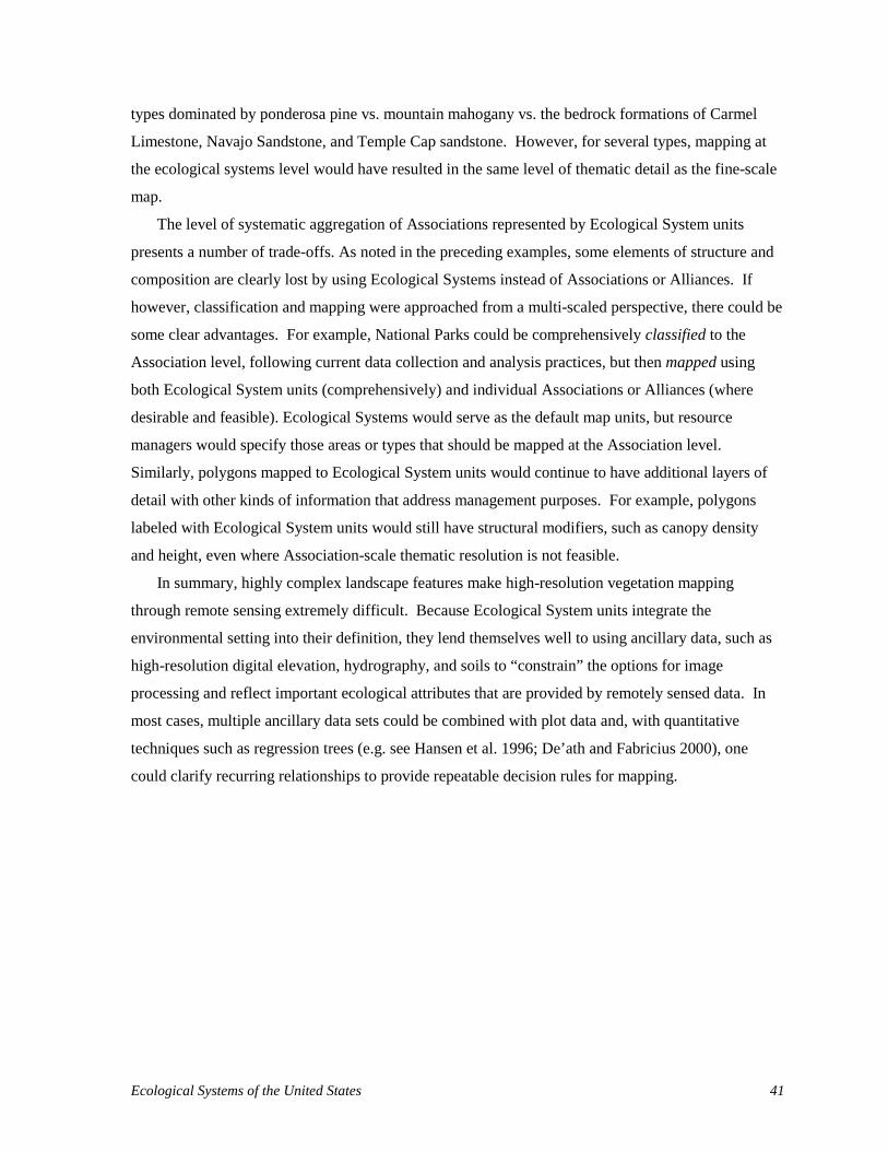
Ecological Systems of the United States 41
types dominated by ponderosa pine vs. mountain mahogany vs. the bedrock formations of Carmel
Limestone, Navajo Sandstone, and Temple Cap sandstone. However, for several types, mapping at
the ecological systems level would have resulted in the same level of thematic detail as the fine-scale
map.
The level of systematic aggregation of Associations represented by Ecological System units
presents a number of trade-offs. As noted in the preceding examples, some elements of structure and
composition are clearly lost by using Ecological Systems instead of Associations or Alliances. If
however, classification and mapping were approached from a multi-scaled perspective, there could be
some clear advantages. For example, National Parks could be comprehensively classified to the
Association level, following current data collection and analysis practices, but then mapped using
both Ecological System units (comprehensively) and individual Associations or Alliances (where
desirable and feasible). Ecological Systems would serve as the default map units, but resource
managers would specify those areas or types that should be mapped at the Association level.
Similarly, polygons mapped to Ecological System units would continue to have additional layers of
detail with other kinds of information that address management purposes. For example, polygons
labeled with Ecological System units would still have structural modifiers, such as canopy density
and height, even where Association-scale thematic resolution is not feasible.
In summary, highly complex landscape features make high-resolution vegetation mapping
through remote sensing extremely difficult. Because Ecological System units integrate the
environmental setting into their definition, they lend themselves well to using ancillary data, such as
high-resolution digital elevation, hydrography, and soils to “constrain” the options for image
processing and reflect important ecological attributes that are provided by remotely sensed data. In
most cases, multiple ancillary data sets could be combined with plot data and, with quantitative
techniques such as regression trees (e.g. see Hansen et al. 1996; De’ath and Fabricius 2000), one
could clarify recurring relationships to provide repeatable decision rules for mapping.

42 NatureServe
Applications to Management and Monitoring Having mapped ecological systems and established occurrences on the ground, we want to know if
each mapped occurrence is of sufficient quality (viability or ecological integrity) or can feasibly be
restored to such quality. This is the next essential step towards developing local-area management
and monitoring objectives. Characterizing and evaluating the quality of an occurrence provides the
basis for assessing ecological stresses—the degradation, or impairment—of element occurrences at a
given site. There are three core components of occurrence evaluation that can be applied to all focal
conservation elements in a conservation site of any scale – whether these are individual populations
or species, assemblages of species, ecological communities, or ecological systems. These core
components and their function are as follows:
1) Key Ecological Attributes – structure, composition, interactions and abiotic and biotic processes
that enable the Element Occurrence to persist.
2) Indicator – measurable entity that is used to assess the status and trend of a Key Ecological
Attribute.
3) Indicator rating – the point within a given expected range of variation one would rate each
Indicator that describes its current status.
To assess the quality of element occurrences, one must first identify and document a limited number
of key ecological attributes that support them (the terms “key ecological attribute” and “indicators”
are comparable to the term “ecological attributes” and “indicator” used by TNC in Parrish et al. 2003
and by the EPA publication of Young and Sanzone 2002). After these are identified, a set of
measurable indicators are established to evaluate each attribute and document their expected ranges of
variation. For each indicator, we may then establish thresholds for distinguishing their current status
along a relative scale from “Excellent” to “Poor.”
Documentation of these basic assumptions about key ecological attributes, ranges of variation,
thresholds, and indicators for measurement, are called “Element Occurrence Rank Specifications;”
and form a central component of Heritage methodology. These specifications allow one to
consistently assess whether the attributes exhibited by a given occurrence are within desired ranges or
whether they will require significant effort to be maintained or restored to their desired status. Each
key attribute is reviewed, rated, and then combined with others to rank each occurrence as A
(excellent), B (good), C (fair), and D (poor). The higher the estimated viability or integrity of the

Ecological Systems of the United States 43
occurrence, the higher is its EO rank and presumed conservation value. Table 5 lists the basic EO
Ranks assigned to each occurrence. The break between C and D establishes a minimum quality
threshold for occurrences. D-ranked occurrences are typically presumed to be beyond practical
consideration for ecological restoration. In subsequent management planning, these ranks and
underlying attributes and indicators aid in focusing conservation activities and measuring progress
toward the local conservation objectives.
Table 5. Basic Element Occurrence Ranks
EO Rank Description of Ecological Integrity
A excellent
B good
C fair
D poor
E verified extant (integrity not assessed)
H historical (not recently located)
X extirpated (no longer extant)
Because EO ranks are used to represent the relative conservation value of an EO as it currently exists,
EO ranks are based solely on attributes that reflect the present status, or quality, of that EO. The three
generalized EO rank categories used to organize the various key ecological attributes are condition,
size, and landscape context. Ranks in each of these categories are combined to arrive at an overall
occurrence rank. Thus:
Condition + Size + Landscape Context ⇒ Estimated Viability or Integrity ≈ EO Rank
For community and system Elements, the term “ecological integrity” is preferable to that of viability
(used for species), since communities and systems are comprised of many separate species, each with
their own viability. Ecological integrity is the “maintenance of…structure, species composition, and
the rate of ecological processes and functions within the bounds of normal disturbance regimes3.
More directly, EO ranks reflect the degree of negative anthropogenic impact to a community or
3From. Lindenmayer and Recher (in Lindenmayer and Franklin 2002). Similarly, Karr and Chu (1995) define ecological (or biological) integrity as “the capacity to support and maintain a balanced, integrated, adaptive biological system having the full range of elements (genes, species, and assemblages) and processes (mutations, demography, biotic interactions, nutrient and energy dynamics, and metapopulation processes) expected in the natural habitat of a region.

44 NatureServe
system (i.e., the degree to which people have directly or indirectly adversely or favorably impacted
community composition, structure, and/or function, including alteration of natural disturbance
processes).
It is not necessary to have knowledge of all factors in each of the three rank categories to develop EO
rank specifications. The three EO rank factor categories and generalized key attributes are
summarized in Table 6 below.
Table 6. Element Occurrence Rank Categories and Key Ecological Attributes
CATEGORY GENERALIZED KEY ECOLOGICAL ATTRIBUTES (examples of indicators are noted within parentheses)
Species Communities and Systems
reproduction and health (evidence of regular, successful reproduction; age distribution for long-lived species; persistence of clones; vigor, evidence of disease affecting reproduction/survival)
√
development/maturity (stability, presence of old-growth)
√
species composition and biological structure (richness, evenness of species distribution, presence of exotics)
√ √
ecological processes (degree of disturbance by logging, grazing; changes in hydrology or natural fire regime)
√ √
Condition
abiotic physical/chemical attributes (stability of substrate, physical structure, water quality) [excluding processes]
√ √
area of occupancy √ √ population abundance √
population density √ Size
population fluctuation (average population and minimum population in worst foreseeable year)
√
landscape structure and extent (pattern, connectivity, e.g., measure of fragmentation/ patchiness, measure of genetic connectivity)
√ √
Landscape Context condition of the surrounding landscape
(i.e., development/maturity, species composition and biological structure, ecological processes, abiotic physical/chemical attributes)
√ √
Indicators. Key Ecological Attributes may be difficult or impossible to directly measure. Where this
is the case, an indicator of the Attribute that may be reasonably and effectively measured should be
identified. In a river floodplain system, for example, river flow dynamics may be an ecological
process tha is a Key Ecological Attribute, but it is not reasonable to expect that every possible

Ecological Systems of the United States 45
parameter would be measured. A few parameters (e.g., flood seasonality and periodicity) can be
selected that will give us an overall indication (indicator) of how the status of our Key Attribute (flow
dynamics) is changing. So the indicator may be a subset of the variables defining the Key Attribute,
or a more measurable substitute for the Attribute.
Any element’s Key Ecological Attributes (and therefore their indicators) will vary over time in a
relatively undisturbed setting. This variation is not random, but falls within a range that we recognize
as either a) natural and consistent with the long-term persistence of each occurrence, or b) outside the
natural range because of human influences (e.g., fire suppression in fire adapted systems).
Establishing Thresholds. To effectively evaluate occurrences relative to each other, overall
ecological integrity ranks should establish a scale for distinguishing between “A”, “B”, “C”, and “D”
occurrences. This scale should usually spread from a lowermost limit (the “D” rank or minimum EO
threshold) up through the threshold for an “A” rank. In addition, the threshold delineating EOs with
“fair” vs. “poor” viability or integrity must be identified. Figure 10 illustrates the rank scale for “A”,
“B”, “C”, and “D”-ranked EOs.
Figure 10 - Model of the A, B, C, and D Rank Scale
Figure 10. Rank scale for “A”, “B”, “C”, and “D”-ranked EOs.
minimum C rank criteria(C rank threshold)
minimum EO criteria
* within the next 10-25 years, based on historic evidence and current status
minimum A rank criteria(A rank threshold)
criteria for best conceivablyachievable EOs in future*A
B
C
D
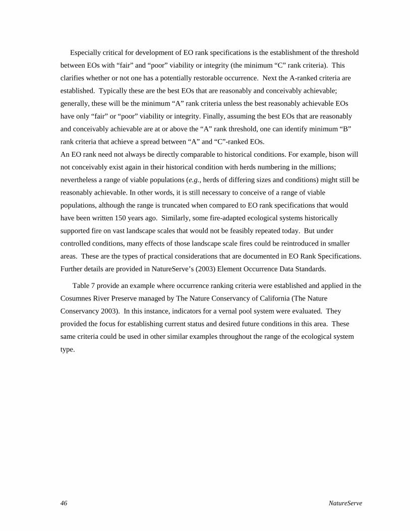
46 NatureServe
Especially critical for development of EO rank specifications is the establishment of the threshold
between EOs with “fair” and “poor” viability or integrity (the minimum “C” rank criteria). This
clarifies whether or not one has a potentially restorable occurrence. Next the A-ranked criteria are
established. Typically these are the best EOs that are reasonably and conceivably achievable;
generally, these will be the minimum “A” rank criteria unless the best reasonably achievable EOs
have only “fair” or “poor” viability or integrity. Finally, assuming the best EOs that are reasonably
and conceivably achievable are at or above the “A” rank threshold, one can identify minimum “B”
rank criteria that achieve a spread between “A” and “C”-ranked EOs.
An EO rank need not always be directly comparable to historical conditions. For example, bison will
not conceivably exist again in their historical condition with herds numbering in the millions;
nevertheless a range of viable populations (e.g., herds of differing sizes and conditions) might still be
reasonably achievable. In other words, it is still necessary to conceive of a range of viable
populations, although the range is truncated when compared to EO rank specifications that would
have been written 150 years ago. Similarly, some fire-adapted ecological systems historically
supported fire on vast landscape scales that would not be feasibly repeated today. But under
controlled conditions, many effects of those landscape scale fires could be reintroduced in smaller
areas. These are the types of practical considerations that are documented in EO Rank Specifications.
Further details are provided in NatureServe’s (2003) Element Occurrence Data Standards.
Table 7 provide an example where occurrence ranking criteria were established and applied in the
Cosumnes River Preserve managed by The Nature Conservancy of California (The Nature
Conservancy 2003). In this instance, indicators for a vernal pool system were evaluated. They
provided the focus for establishing current status and desired future conditions in this area. These
same criteria could be used in other similar examples throughout the range of the ecological system
type.

47
Tab
le 7
. Par
tial
EO
Ran
k do
cum
ent f
or th
e N
orth
ern
Cal
ifor
nia
Har
dpan
Ver
nal P
ool m
odif
ied
from
the
Con
sum
nes
Riv
er P
rese
rve
Pla
n of
The
N
atur
e C
onse
rvan
cy o
f Cal
ifor
nia.
Key
Eco
logi
cal
Att
ribu
te
Indi
cato
rs
Indi
cato
r R
atin
gs
Cat
egor
ical
Cur
rent
sta
te: s
hade
d; I
tali
cs =
Des
ired
Rat
ing
B
asis
for
Rat
ing
Via
bilit
y O
bjec
tive
Cur
rent
St
atus
[D
ate]
Bas
is fo
r C
urre
nt
Stat
us R
atin
g C
ateg
ory
Poo
r F
air
Goo
d V
ery
Goo
d
L
ands
cape
C
onte
xt
Fire
Are
a-In
tens
ity
Reg
ime
Buf
fer
arou
nd
vern
al p
ool
com
plex
that
can
be
fir
e m
anag
ed
< 0
.25
mile
buf
fer
0.25
- 0
.49
mile
buf
fer
0.5
– 0.
99 m
ile b
uffe
r >
1 m
ile
buff
er o
ver
>80
% o
f the
per
imet
er o
f ve
rnal
poo
l pro
pert
ies
Mar
ty (
TN
C)
2001
M
aint
ain
a bu
ffer
of
≥ 1
mile
ar
ound
ver
nal
pool
com
plex
on
larg
e ve
rnal
poo
l tr
acts
1 m
i buf
fer
inta
ct a
roun
d H
owar
d an
d Sc
hnei
der
Ran
ches
(20
01)
Ana
lysi
s of
re
mot
e se
nsin
g da
ta
Lan
dsca
pe
Con
text
Fi
re A
rea-
Inte
nsity
R
egim
e
Fire
ret
urn
inte
rval
and
are
a bu
rned
Fire
ret
urn
inte
rval
< 1
ye
ar o
r >
10
year
s fo
r >
10
% o
f th
e ve
rnal
poo
l gr
assl
and.
Fire
ret
urn
inte
rval
be
twee
n 7-
10 y
ears
for
>
10%
of
the
vern
al p
ool
gras
slan
d.
Fire
ret
urn
inte
rval
be
twee
n 5-
7 ye
ars
for
>
50%
of
the
vern
al p
ool
gras
slan
d.
Fir
e re
turn
inte
rval
be
twee
n 3-
5 ye
ars
for
>
80%
of t
he v
erna
l poo
l gr
assl
and.
Mar
ty (
in p
rep)
20
01; R
. Will
s pe
rs. c
omm
.; Po
llak
and
Kan
19
98;
Men
ke19
92
Mai
ntai
n a
pres
crib
ed f
ire
retu
rn in
terv
al o
f 3-
5 ye
ars
for
over
80
% o
f th
e ve
rnal
po
ol g
rass
land
s on
the
Pres
erve
.
> 1
0 ye
ar f
ire
retu
rn in
terv
al
for
> 1
0% o
f th
e Pr
eser
ve’s
ve
rnal
poo
l gr
assl
ands
His
tori
cal f
ire
data
Lan
dsca
pe
Con
text
C
onne
ctiv
ity
of
vern
al p
ool
com
plex
es
Dis
trib
utio
n of
la
nd p
erm
anen
tly
prot
ecte
d
< 1
0% c
onne
ctiv
ity
10-4
9% c
onne
ctiv
ity
50-7
4% c
onne
ctiv
ity
N
ote:
15-
25,0
00 a
c w
ould
be
prot
ecte
d w
ith
this
con
nect
ivity
to b
e ra
ted
Goo
d.
75%
or
high
er
conn
ecti
vity
CR
P Pl
anni
ng
Tea
m 2
000;
T
his
Land
. C
onte
xt is
link
ed
to th
e ar
ea
prot
ecte
d un
der
Size
, bel
ow.
Est
ablis
h 75
%
conn
ecti
vity
of
prot
ecte
d ve
rnal
po
ol h
abita
t by
2005
> 5
0%
conn
ecti
vity
(D
E. 2
001)
Act
ual l
and
or
ease
men
t pu
rcha
ses
Con
diti
on
Nat
ive
spec
ies
dive
rsity
N
ativ
e sp
ecie
s co
ver
Rel
ativ
e na
tive
spe
cies
co
ver
(RN
SC)
in v
erna
l po
ols
< 8
0%
RN
SC in
ver
nal p
ools
80-
84%
R
NSC
in v
erna
l poo
ls 8
5-90
%
RN
SC in
ver
nal p
ools
>
90%
M
onit
orin
g da
ta
– M
arty
(20
01)
Mai
ntai
n re
lati
ve
nati
ve s
peci
es
cove
r >9
0% in
ve
rnal
poo
ls
How
ard
Ran
ch
mea
n-90
%,
se=
1.7%
; V
alen
sin
Ran
ch
–Mea
n=84
%,
se=
3% (
2001
)
Mon
itor
ing
data
(M
arty
200
1)
Con
diti
on
Nat
ive
spec
ies
dive
rsity
na
tive
spe
cies
ri
chne
ss
Ric
hnes
s on
poo
l edg
e <5
sp
ecie
s/qu
adra
t (35
cm
x
70 c
m)
Ric
hnes
s on
poo
l edg
e 6-
8 sp
ecie
s/qu
adra
t R
ichn
ess
on p
ool e
dge
9-10
spe
cies
/qua
drat
R
ichn
ess
on p
ool e
dge
>10
spe
cies
/qua
drat
M
onit
orin
g da
ta
– M
arty
(20
01)
Mai
ntai
n av
erag
e na
tive
spe
cies
ri
chne
ss o
n th
e po
ol e
dge
>10
spec
ies/
quad
rat
How
ard
Ran
ch
mea
n-10
.4,
se=
0.32
; V
alen
sin
Ran
ch
–Mea
n=9.
4,
se=
0.34
(20
01)
Mon
itor
ing
data
(M
arty
200
1)
Con
diti
on
Polli
nati
on
over
all
?
See
rege
nera
tion
of
spe
cies
but
po
pula
tion
s ar
e he
avily
fr
agm
ente
d
Nee
d ba
selin
e da
ta to
det
erm
ine
quan
titat
ive
mea
sure
s fo
r th
is
indi
cato
r –
hold
ex
pert
mee
ting
No
info
rmat
ion
on w
hat o
r ho
w
to m
easu
re.
Iden
tify
exp
erts
an
d ho
ld
mee
ting:
200
3.
Size
Si
ze o
f ve
rnal
po
ol c
ompl
exes
A
cres
of
land
pe
rman
ently
pr
otec
ted
thro
ugh
cons
erva
tion
ea
sem
ent o
r ot
her
< 1
0,00
0 ac
res
prot
ecte
d,
10,0
00 to
15,
000
ac
prot
ecte
d
15,0
00 to
25,
000
ac
prot
ecte
d
N
ote:
Thi
s ac
reag
e w
ould
be
pro
tect
ed w
ith 5
0-74
%
conn
ecti
vity
to b
e ra
ted
Goo
d.
30,0
00 a
c pr
otec
ted
CR
P Pl
anni
ng
Tea
m 2
000;
T
his
Size
is
link
ed to
the
conn
ecti
vity
un
der
Land
. C
onte
xt, a
bove
.
Prot
ect 3
0,00
0 ac
of
ver
nal p
ool
habi
tat w
ith 7
5%
in la
rge,
co
ntig
uous
pa
rcel
s by
200
5
17,0
00 a
c pr
otec
ted
(Dec
. 20
01)
Act
ual l
and
or
ease
men
t pu
rcha
ses

48 NatureServe
Applications to Habitat Modeling
Biologists have long used knowledge of an animal’s habitat to predict its presence or absence.
Numerous approaches to mapping species habitat are well summarized by Scott et al. (2002). Most
traditional methods rely only on the location or observation of specimens and include no information on
the ecological conditions, such as vegetation and climate variables. Using terrestrial ecological system
units as a surrogate to map presence or absence of species habitat has limitations but also provides
enhancement over many traditional methods. Because the process would not rely solely on known locality
records, unsampled areas can be included in predicted models. Coupling known locations with those
predicted from ecological system units, and other ancillary data sets, could lead to more refined maps of
species distribution. Given the national scope of this classification, this approach can now be applied
consistently across the nation.
Several factors complicate the use of any type of vegetation or habitat map to predict species presence
and absence (Scott et al. 2002). For example, birds respond as much or more to vegetation structure than
to floristics. NVC alliance units integrate vegetation structure with composition, and have been shown to
provide useful predictors of songbird habitat. However, there are also many examples where other
environmental factors, such as the presence of steep cliffs or canyons, in association with certain
vegetation or water sources, better characterize specific habitat. Species associated with certain
hydrologic regimes can be falsely predicted or overestimated unless hydrology and/or riparian habitats are
incorporated as linear map features. Habitat for fossorial rodents can also be poorly predicted if
vegetation maps do not integrate soil characteristics very well. Terrestrial ecological systems integrate
regional climate, local landform, some soil characteristics, as well as local patterns in vegetation and
structure into their definition. By mapping ecological system units, many common attributes of wildlife
habitat may be better expressed.
Another complication in habitat modeling arises from the variation in specificity of habitat
requirements among different species. Some species are generalists in their habitat. Others are restricted
to narrow habitat types. In addition, our ability to map certain habitat characteristics can often surpass
our knowledge of habitat requirements for many species. As a result, classifications of wildlife habitat
vary significantly in the scope and concept of units described. They also vary from state to state, or
among different land managing agencies. Ecological system units are more consistently defined in terms
of concept and fall into repeatable categories of spatial scale. They may be useful for “crosswalking”
among existing habitat classification systems within and across jurisdictions. Appendix 4 includes an
example where some 110 ecological system units that fall within California are crosswalked with the 53
wildlife habitat relationship classes of Mayer and Laudenslayer (1988). Given the likelihood that all 110

Ecological Systems of the United States 49
ecological system units could be mapped across the state of California and into adjacent states, these units
should provide significant utility for wildlife assessment.
Avenues for Classification Refinement As stated previously, ecological classification ideally proceeds through several phases in a continual
process of refinement. These phases include 1) literature review and synthesis of current knowledge, 2)
formulating initial hypotheses and tentatively describing each type, that support 3) establishing a field
sample design, 4) gathering of field data, 5) data analysis and interpretation, 6) description of types, 7)
establishing dichotomous keys to classification units, 8) mapping of classification units, and 9) refinement
of the classification.
In preceeding sections, we demonstrated how ecological system units can be inventoried and mapped,
using existing methodologies and mapped data, at both regional and local scales. These results indicate
both the potential utility of ecological system units and a number of directions for their refinement.
Mapping ecological systems serves as an immediate test of classification concepts, ensuring that the
mapped area is treated comprehensively by the classification, providing for a consistent use of multiple
spatial data, and clarifying distinctions between types. Regional mapping provides an initial coverage of
system distribution based primarily on the date of remotely sensed imagery. Depending on the ancillary
data sets used in map development, these maps may be overlain with other independently derived spatial
data, such as elevation, landforms, geology, soils, etc, to further describe the distribution, environmental
setting, and landscape patterns that characterize each system type. These maps, if derived using several
year-old remotely-sensed imagery, should also function as a practical basis for sample design to gather
“training” data for mapping with new imagery.
As noted by Jennings et al. (2003), a vegetation association or community represents a statistical and
conceptual synthesis of floristic patterns (Westhoff and van der Maarel 1973, Mueller-Dombois and
Ellenberg 1974, Kent and Coker 1992). It is an abstraction, representing a defined range of floristic,
structural, and environmental variability. Ecological systems represent a similar kind of abstraction that
encompasses the concepts of multiple vegetation associations, and emphasizes the environmental
attributes that result in their co-occurrence on the ground. The definition of both associations and
ecological systems as individual types is the result of a set of classification decisions based on field
sampling, data analysis and interpretation. Suggested approaches to these phases are well summarized by
Jennings et al. (2003) for application to vegetation classification.
Two criteria must be met in order for any analysis to be robust. First, the samples must represent a
wide range of the compositional, structural, and environmental variation of the proposed type or group of
closely related types. Second, there must be a sufficient level of redundancy in the samples to statistically

50 NatureServe
identify mutually exclusive clusters in the data. Standardized approaches for defining ecological system
units follows closely from those for vegetation units, but with important caveats. For example, although
one should take field sample plots within relatively homogeneous vegetation patches, sampling for
ecological system units should consider use of transect-based or other sub-sample plot designs to allow
for consistent samples of several component associations and document associations in similar
environments that make up the ecological system occurrence (see Whittaker 1975).
Measurement of the similarity or dissimilarity among the field samples is central to most
classification approaches. A number of quantitative methods for evaluating beta diversity - in terms of
turnover in species presence/absence - are commonly applied in vegetation studies (Wilson and Schmida
1984, Magurran 1988), and these could be applied to the data from sub-sample designs. Other
quantitative approaches allow for integration of multiple factors, such as relative abundance of vegetation
or environmental variables, into more abstract multi-scale information statistics that support analyses
better suited to ecosystem classification (Loehle and Wein 1994). Existing data, combined from various
sources, are often too heterogeneous to be usable in these quantitative analyses, but such analyses should
be considered when designing future sampling.

Ecological Systems of the United States 51
Conclusions
This report presents work conducted to classify and describe terrestrial ecological systems in the
coterminous United States and southern Alaska, and adjacent portions of Mexico and Canada (including
coastal British Columbia). A terrestrial ecological system is defined as a group of plant community types
(associations) that tend to co-occur within landscapes with similar ecological processes, substrates, and/or
environmental gradients. A given terrestrial ecological system will typically manifest itself in a landscape
at intermediate geographic scales of 10s to 1,000s of hectares and persist for 50 or more years.
The classification produced here is at a “meso-scale,” both spatially and temporally, and the specific
spatial and temporal scales are further refined by the biotic and ecological distinctiveness of the system.
Our goal was to provide a set of such system types for conservation and resource management
applications. Other classifications, which are typically hierarchically arranged, do well at either micro or
macro scales. We show how our classification both relies on those efforts and can be linked to them. In
fact, the floristic units of the IVC/NVC are an integral part of defining the concepts and spatial limits of
the system types. At this time, we focus on a single system level, defined by modular diagnostic
classifiers that help to describe the essential ecological and vegetational characteristics of the type. We
used an expert-based approach to define a “working set” of system types, and outline further steps for
their ongoing development.
This effort resulted in the identification and description of 599 upland and wetland ecological system
types within the project area. They represent the full range of natural gradients, with some 381 types
(63%) being uplands, 183 types (31%) being wetland, and 35 types (6%) being complexes of uplands and
wetlands. Excluding upland/wetland complexes, some 322 types (54%) are predominantly forest,
woodland, and/or shrubland, and some 166 types (28%) are predominantly herbaceous, savanna, or shrub
steppe. Seventy-four types (12%) are sparsely vegetated or “barren.”
Terrestrial ecological system units provide practical, systematically defined groupings of plant
community types that can enhance the mapping of terrestrial communities and ecosystems at multiple
scales of spatial and thematic resolution. We provide a number of applications of ecological system units
to conservation assessment, ecological inventory, mapping, land management, ecological monitoring, and
species habitat modeling. The classification, referred to as the U.S. Terrestrial Ecological Systems
Classification, is the U.S. component of an International Terrestrial Ecological Systems Classification.
NatureServe and partners will facilitate continued development and refinement of this classification.

52 NatureServe
Literature Cited Albert, D. A. 1995. Regional Landscape Ecosystems of Michigan, Minnesota, and Wisconsin: A
Working Map and Classification. U.S. Forest Service General Technical Report NC-178. North Central Forest Experiment Station, St. Paul, Minnesota, USA.
Anderson, M., P. Comer, D. Grossman, C. Groves, K. Poiani, M. Reid, R. Schneider, B. Vickery, and A.
Weakley. 1999. Guidelines for Representing Ecological Communities in Ecoregional Plans. The Nature Conservancy.
Austin, M. P. 1985. Continuum concept, ordination methods and niche theory. Annual Review of
Ecology and Systematics 16: 39-61. __________. 1991. Vegetation Theory in Relation to Cost-Efficient Surveys. Pages 17–22 In C.R.
Margules, and M.P. Austin, Editors. Nature Conservation: Cost Effective Biological Surveys and Data Analysis. CSIRO Publishing, Collingwood, Victoria, Australia.
Austin, M. P. and P. C. Heyligers. 1989. Vegetation survey design for conservation: gradsect sampling of
forests in Northeastern New South Wales. Biological Conservation 50: 13-32. Austin, M. P. and T. M. Smith. 1989. A new model for the continuum concept. Vegetatio 83: 35-47. Avers, P. E., D. T. Cleland, W. H. McNab, M. E. Jensen, R. G. Bailey, T. King, C. B. Goudey, and W. E.
Russell. 1994. National Hierarchical Framework of Ecological Units. U.S. Forest Service, Washington, D.C., USA.
Bailey, R.G. 1995. Description of the Ecoregions of the United States. U.S. Forest Service
Miscellaneous Publication 1391 (Revised), with Separate Map at a Scale of 1:7,500,000, Washington, D.C., USA.
________. 1996. Ecosystem Geography. Springer-Verlag New York Inc., New York. ________. 1998. Ecoregion Map of North America: Explanatory Note. USDA Forest Service Misc.
Publication No. 1548. 10 pp. + map [Scale 1:15,000,000]. Barnes, B.V. 1984. Forest Ecosystem Classification in Baden-Wurtenburg, Germany. In: J.G. Bockheim
(Ed.) Symposium Proceedings Forest Land Classification: Experience, Problems, Perspectives. NCR-102 North Central Forest Soils Com. Soc. Amer. For., USDA Forest Service and USDA Soil Conservation Service. Madision WI.
Barnes, B.V., D.R. Zak, S.R. Denton, and S.H. Spurr. 1998. Forest Ecology, Fourth Edition. John Wiley
and Sons, New York. Beissinger, S.R., and M.I. Westphal. 1998. On the use of demographic models of population viability in
endangered species management. Journal of Wildlife Management 62: 821-841. Braun-Blanquet, J. 1964. Pflanzensoziologie, Grundzüge der Vegetationskunde. Springer-Verlag, Vienna,
Austria.

Ecological Systems of the United States 53
Brinson, M. M. (1993). A Hydrogeomorphic Classification for Wetlands. Technical Report WRP-DE-4, U.S. Army Engineer Waterways Experiment Station, Vicksburg, MS. NTIS No. AD A270 053.
Brown, D. E., F. Reichenbacher, S.E. Franson. 1998. A Classification of North American Biotic
Communities. University of Utah Press. Salt Lake City. Brown, D.E., C.H. Lowe, and C.P. Pase. 1980. A digitized systematic classification for ecosystems with
an illustrated summary of the natural vegetation of North America. USDA Forest Service General Technical Report RM-73. Rocky Mountain Forest and Range Experiment Station, Fort Collins, Colorado, USA.
Carroll, C., R.F. Noss, and P.C. Paquet. 2001. Carnivores as focal species for conservation planning in
the Rocky Mountain region. Ecological Applications 11: 961-980. Cleland, D.T.; P.E. Avers, W.H. McNab, M.E. Jensen, R.G. Bailey, T. King, and W.E. Russell, 1997.
National Hierarchical Framework of Ecological Units. Pp. 181-200 in: Boyce, M. S.; Haney, A. (eds.), Ecosystem Management Applications for Sustainable Forest and Wildlife Resources. Yale University Press, New Haven.
Clements, F. E. 1916. Plant Succession: An Analysis of the Development of Vegetation. Carnegie
Institute of Washington Publication, Washington, D.C. Cogan, D., M. Reid, J. Von Loh, and K. Schulz. 2002. USGS-NPS Vegetation Mapping Program, Zion
National Park (Final Report). Technical Memorandum No. 8260-02-06. U.S. Bureau of Reclamation Technical Service Center. Denver, Colorado.
Comer, P., S. Menard, M. Tuffly, K. Kindscher, R. Rondeau, G. Jones, G. Steinuaer, D. Ode, R.
Schneider, and D. Grossman. 2003. Upland and Wetland Ecological Systems in Colorado, Wyoming, South Dakota, Nebraska, and Kansas. Report and map to the National Gap Analysis Program. Dept. of Interior USGS. NatureServe, Arlington, Virginia.
Comer, P.J., M.S. Reid, R.J. Rondeau, A. Black, J. Stevens, J. Bell, M. Menefee, and D. Cogan. 2002. A
Working Classification of Terrestrial Ecological Systems in the Northern Colorado Plateau: Analysis of their Relation to the National Vegetation Classification and Application to Mapping. NatureServe. Report to the National Park Service.
Comer, P.J., D.A. Albert, H.A. Wells, B.L. Hart, J.B. Raab, D.L. Price, D.M. Kashian, R.A. Corner and
D.W. Schuen. 1995. Michigan’s Native Landscape, as Interpreted from the General Land Office Surveys 1816-1856. Report to the U.S. E.P.A. Water Division and the Wildlife Division, Michigan Department of Natural Resources. Michigan Natural Features Inventory, Lansing, MI.
Cowardin, L. W., V. Carter, F.C. Golet, and E. T. LaRoe. 1979. Classification of wetlands and
deepwater habitats of the United States. Biological Service Program, U.S. Fish and Wildlife Service, FWS/OBS 79/31. Office of Biological Services, Fish and Wildlife Service, U.S. Department of Interior, Washington, D.C.
Curtis, J.T. 1959. The Vegetation of Wisconsin: An Ordination of Plant Communities. University of
Wisconsin Press, Madison.
Daubenmire, R.F. 1952. Forest vegetation of northern Idaho and adjacent Washington, and its bearing on concepts of vegetation classification. Ecological Monographs 22: 301-330.

54 NatureServe
Daubenmire, R. 1966. Vegetation: identification of typal communities. Science 151: 291-298. Davies, C. and D. Moss. 1999. EUNIS Habitat Classification. Final Report to the European Topic Center On
Nature Conservation, European Environment Agency. November 1999. Huntington: Institute Of Terrestrial Ecology.
Delcourt H.R., and P.A. Delcourt. 1988. Quaternary landscape ecology: relevant scales in space and time.
Landscape Ecology 2: 23-44. De’Ath, G. and K.E. Fabricius. 2000. Classification and regression trees: a powerful yet simple technique
for ecological data analysis. Ecology 81: 3178-3192. Devillers, P., J. Devillers-Terschuren, and J. P. Ledant. 1991. CORINE biotopes manual. Habitats of the
European Community. Data Specifications – Part 2. Luxembourg: Office for Official Publications of the European Communities.
Digregorio, A. and L.J.M Jansen. 2000. Land Cover Classification System (LCCS): Classification
Concepts and User Manual. Environment and Natural Resources Service, GCP/RAF/287/ITA Africover - East Africa Project and Soil Resources, Management and Conservation Service. FAO, Rome.
Driscoll, R.S., D.L. Merkel, D.L. Radloff, D.E. Snyder, and J.S. Hagihara. 1984. An ecological land
classification framework for the United States. U.S. Department of Agriculture, Forest Service, Miscellaneous Publication 1439, Washington, D.C.
Edwards, T.C., Jr., C.H. Homer, S.D. Bassett, A. Falconer, R.D. Ramsey, and D.W. Wight. 1995. Utah
Gap Analysis: An Environmental Information System. Final Project Report 95-1, Utah Cooperative Fish and Wildlife Research Unit, Utah State University, Logan.
Eyre, F.H., editor. 1980. Forest cover types of the United States and Canada. Society of American
Foresters, Washington, D.C. Faber-Langendoen, D., J. Drake, L. Sneddon, K. Schulz, and R. White. 2002 Draft. Field Methods for
Vegetation Mapping. U.S. Geological Survey – National Park Service Vegetation Mapping Program. Natureserve, Arlington Virginia.
Federal Geographic Data Committee. 1997. Vegetation Classification Standard, FGDC-STD-005. Web
Address: http://www.fgdc.gov/standards/documents/standards/vegetation/vegclass.pdf. Flahault, C. and C. Schröter. 1910. Phytogeographische Nomenklatur. Berichte und Anträge 3. Third
International Congress of Botany. Brussels, Belgium. Fleishman, E., R.B. Blair, and D.D. Murphy. 2001. Empirical validation of a method for umbrella
species selection. Ecological Applications 11: 1489-1501. Frost, C.C. 1998. Presettlement Fire Frequency Regimes of the United States: A First Approximation.
Pages 70-81 IN: Pruden, T.L., and L.A. Brennan, Eds. 1998. Fire in Ecosystem Management: Shifting the Paradigm from Suppression to Prescription. Tall Timbers Fire Ecology Conference Proceedings, No.20. Tall Timbers Research Station, Tallahassee, FL.

Ecological Systems of the United States 55
Gillison, A.N., and K.R.W. Brewer. 1985. The use of gradient directed transects or gradsects in natural resource surveys. Journal of Environmental Management 20: 103-127.
Gleason, H. A. 1926. The individualistic concept of the plant association. Bulletin Of The Torrey
Botanical Club 53: 7-26.
Golley, F. B. 1993. History of the Ecosystem Concept in Ecology. Yale University Press, New Haven. Grossman, D.H., K.L. Goodin, Xiaojun Li, D. Faber-Langendoen, M. Anderson, P. Bourgeron, and R.
Vaughn. 1994. Field Methods For Vegetation Mapping. NBS/NPS Vegetation Mapping Program. The Nature Conservancy, Arlington, VA, and Environmental Systems Research Institute, Redlands, CA.
Grossman, D.H., D. Faber-Langendoen, A.W. Weakley, M. Anderson, P. Bourgeron, R. Crawford, K.
Goodin, S. Landaal, K. Metzler, K.D. Patterson, M. Pyne, M. Reid, and L. Sneddon. 1998. International Classification Of Ecological Communities: Terrestrial Vegetation Of The United States. Volume I: The National Vegetation Classification Standard. The Nature Conservancy, Arlington, VA. 92 Pp.
Groves, C.R., D.B. Jensen, L.L. Valutis, K.H. Redford, M.L. Shaffer, J.M. Scott, J.V. Baumgartner, J.V.
Higgins, M.W. Beck, and M.G. Anderson. 2002. Planning for biodiversity conservation: putting conservation science into practice. Bioscience 52: 499-512.
Hall, J., P. Comer, A. Gondor, R. Marshall, S. Weinstein. 2001. Conservation Elements of the Barry M.
Goldwater Range, Arizona: Characteristics, Status, Threats, and Preliminary Management Recommendations. The Nature Conservancy Of Arizona.
Hansen, M., R. Dubayah, and R. Defries. 1996. Classification trees: an alternative to traditional land
cover classifiers. International Journal Of Remote Sensing Vol. 17, No. 5, Pp. 1075-1081. Haufler, J.B., C.A. Mehl, and G.J. Roloff. 1996. Using a coarse filter approach with species assessment
for ecosystem management. The Wildlife Society Bulletin 24: 200-208. Jenkins, R.E. 1976. Maintenance of natural diversity: approach and recommendations. Pp 441-451. In
proceedings of the Forty-first North American Wildlife and Natural Resources Conference, Washington, D.C.
Jenkins, R.E. 1985. The identification, acquisition, and preservation of land as a species conservation
strategy. Pp. 129-145. In R.J. Hoage, ed. Animal Extinctions. Smithsonian Institution Press, Washington, D.C.
Jennings, M., O. Loucks, D. Glenn-Lewin, R. Peet, D. Faber-Langendoen, D. Grossman, A. Damman, M.
Barbour, R. Pfister, M. Walker, S. Talbot, J. Walker, G. Hartshorn, G. Waggoner, M. Abrams, Alison Hill, David Roberts, David Tart. 2003. Guidelines for Describing Associations and Alliances of The U.S. National Vegetation Classification. The Ecological Society of America Vegetation Classification Panel, Version 2.0. March 28, 2003.
Johnson, K.N., F. Swanson, M. Herring, and S. Greene. 1999. Bioregional assessments: Science at the
crossroads of management and policy. Island Press, Washington DC.

56 NatureServe
Karr, J.R. and E.W. Chu. 1995. Ecological integrity: Reclaiming lost connections. pp. 34-48. In L. Westra and J. Lemons (eds). Perspectives on Ecological Integrity. Kluwer Academic, Dordrecht, Netherlands.
Kartesz, J. T. 1999. A Synonymized Checklist and Atlas With Biological Attributes for The Vascular
Flora of The United States, Canada, and Greenland. First Edition. In: J. T. Kartesz and C. A. Meacham. Synthesis of The North American Flora, Version 1.0. North Carolina Botanical Garden, Chapel Hill, NC.
Kent, M. and P. Coker. 1992. Vegetation description and analysis: A practical approach. Belhaven Press.
London, UK. Kimmins, J.P. 1997. Forest Ecology: A Foundation for Sustainable Management. Second Edition.
Prentice Hall, Upper Saddle River, New Jersey. King, A.W. 1993. Consideration of scale and hierarchy. Pp 19-45. In S. Woodley, J. Kay and G. Francis
(eds.). Ecological integrity and the mangement of ecosystems. St. Lucie Press. Kintsch, J.A. and D. L. Urban. 2002. Focal species, community representation, and physical proxies as
conservation strategies: a case study in the Amphibolite Mountains, North Carolina, U.S.A. Conservation Biology 16: 936-947.
Kuchler, A.W. 1988. Ecological Vegetation Maps and Their Interpretation. Pp. 469–480. In: A.W. Kuchler
and I.S. Zonneveld (Eds.). Vegetation Mapping,. Kluwer Academic Publishers, Boston. Lapin, M. and B.V. Barnes. 1995. Using a landscape ecosystems approach to assess species and ecosystem
diversity. Conservation Biology 9: 1148-1158. Lincoln, R.J., G. A. Boxshall, and P.F. Clark. 1982. A dictionary of ecology, evolution, and systematics.
Cambridge University Press, New York. Lindenmayer, D.B. and J.F. Franklin. 2002. Conserving forest biodiversity: A comprehensive
multiscaled approach. Island Press, Washington, DC. Loehle, C., and G. Wein. 1994. Landscape habitat diversity: A multi-scale information theory approach.
Ecological Modeling 73: 311-329. Magurran, A.E. 1988. Ecological Diversity and its Measurement. Princeton University Press, Princeton, NJ. Marshall, R.M., S. Anderson, M. Batcher, P. Comer, S. Cornelius, R. Cox, A. Gondor, D. Gori, J. Humke,
R. Paredes Aquilar, I.E. Parra, and S. Schwartz. 2000. An Ecological Analysis of Conservation Priorities in the Sonoran Desert Ecoregion. Prepared By The Nature Conservancy Arizona Chapter, Sonoran Institute, and Instituto Del Medio Ambiente y El Desarrollo Sustentable del Estado de Sonora, with support from Department of Defense Legacy Program, Agency and Institutional Partners.
Master, L. L., L. E. Morse, A. S. Weakley, G. A. Hammerson, and D. Faber-Langendoen. 2002. Heritage
conservation status assessment factors. NatureServe, Arlington, Virginia. Mayer, K.E., and W.F. Laudenslayer Jr. (eds.). 1988. A Guide to Wildlife Habitats in California.
California Dept. Wildlife and Wildfire Protection, Sacramento, CA.

Ecological Systems of the United States 57
McCune, B., and M.J. Mefford. 1997. PC-ORD. Multivariate Analysis of Ecological Data, Version 3.0. Mjm Software Design, Gleneden Beach, OR.
McNab, W.H., and P.E. Avers. 1994. Ecological Subregions of the United States: Section Descriptions.
USDA Forest Service, WO-WSA-5. Washington, DC. Menard, S., and C. Lauver, 2002. Using Ecological Systems as land cover map units for GAP. GAP
Bulletin 9: 12. Merriam, C.H. 1898. Life zones and crop zones of the United States. U.S. Department of Agriculture,
Division of Biological Survey, Bulletin 10: 1-79., Washington, D.C. Merrill, E.H., W.A. Reiners, R.W. Marrs, S.H. Anderson, T.W. Kohley, M.E. Herdendorf, and K.L.
Driese. 1996. Wyoming Gap Analysis: A Geographic Analysis of Biodiversity - Final Report, USGS Biological Resources Division. Wyoming Cooperative Fish and Wildlife Research Unit and University of Wyoming, Laramie, WY.
Minnesota Natural Heritage Program (Minnesota Department of Natural Resources). 1993. Minnesota’s
native vegetation: a key to natural communities. Version 1.5. Minnesota Department of Natural Resources Natural Heritage Program, Biological Report No. 20. St. Paul, MN.
Moore, J., C. Rumsey, T. Knight, J. Nachlinger, P. Comer, D. Dorfman, and J. Humke. 2001. Mojave
Desert: An Ecoregion-Based Conservation Blueprint. The Nature Conservancy, Las Vegas, NV. Moravec, J. 1993. Syntaxonomic and nomenclatural treatment of Scandinavian-type associations and
associations. Journal of Vegetation Science 4: 833-838. Mueller-Dombois, D. and H. Ellenberg. 1974. Aims and Methods of Vegetation Ecology. John Wiley,
New York. Nachlinger, J., K. Sochi, P. Comer, G. Kittel, and D. Dorfman. 2001. Great Basin: An Ecoregion-Based
Conservation Blueprint. The Nature Conservancy, Reno, NV. Natural Resource Conservation Service (NRCS). 1998. Keys to Soil Taxonomy. Eighth Edition. Web
address: http://www.pedosphere.com/resources/sg_usa/. NatureServe. 2003. International Vegetation Classification: Terrestrial Vegetation. NatureServe Central
Databases. Natureserve, Arlington, Virginia. NatureServe. 2002. Element Occurrence Data Standards. NatureServe, Arlington, Virginia. Neely, B., P. Comer, C. Moritz, M. Lammert, R. Rondeau, C. Pague, G. Bell, H. Copeland, J. Humke, S.
Spackman, T. Schulz, D. Theobald, and L. Valutis. 2001. Southern Rocky Mountains Ecoregion: An Ecoregional Assessment and Conservation Blueprint. Prepared by The Nature Conservancy with support from the USDA Forest Service, Rocky Mountain Region, Colorado Division of Wildlife, and Bureau of Land Management.
Noss, R.F. 2000. Maintaining integrity in landscapes and ecoregions. Pp. 191-208. In: Pimentel, D., L.
Westra, and R.F. Noss (eds.). 2000. Ecological integrity: Integrating environment, conservation, and health. Island Press, Washington DC.

58 NatureServe
Noss, R.F. and A.Y. Cooperrider. 1994. Saving Nature’s Legacy. Island Press, Washington D.C. Noss, R.F. and R.L. Peters. 1995. Endangered ecosystems: A status report on America's vanishing
habitat and wildlife. Defenders of Wildlife, Washington, D.C.
Odum, E.P. 2001. Concept of Ecosystem. Pp. 205-310. In: Levin, S. (Editor-In-Chief), Encyclopedia of Biodiversity, Volume 2. Academic Press.
Olson, D. M, E. Dinerstein, E. D. Wikramanayake, N.D. Burgess, G.V.N. Powell, E.C. Underwood, J.A. D’Amico, I. Itoua, H.E. Strand, J.C. Morrison, C.J. Loukes, T.F. Allnutt, T.H. Ricketts, Y. Kura, J.F. Lamoreux, W.W. Wettengel, P.Hedao, and K.R. Kassem. 2001. Terrestrial Ecoregions of the World: A New Map of Life on Earth. Bioscience 51: 933-938.
O’Neill, R.V. 2001. Is it time to bury the ecosystem concept? Ecology 82: 3275-3284. Parrish, J.D., D. Braun, and R. Unnasch. 2003 draft. Are we conserving what we say we are?: measuring
ecological integrity in evaluations of protected area management effectiveness. (Draft paper) Pfister, R. D. and S. F. Arno. 1980. Classifying forest habitat types based on potential climax vegetation.
Forest Science 26: 52-70. Poiani, K.A., B.D. Richter, M.G. Anderson, and H.E. Richter. 2000. Biodiversity conservation at
multiple scales: Functional sites, landscapes and networks. Bioscience 50: 133-146. Ponomarenko, S. and R. Alvo. 2000. Perspectives on Developing a Canadian Classification of
Ecological Communities. Canadian Forest Service, Science Branch, Information Report ST-X-18E. Natural Resources Canada, Ottawa.
Racey, G.D., A.G. Harris, J.K. Jeglum, R.F. Foster and G.M. Wickware. 1996. Terrestrial and wetland
ecosites of northwestern Ontario. Ontario Ministry of Natural Resources, Northwestern Science and Technology Field Guide FG-02.
Redford, K.H., P. Coppolillo, E.W. Sanderson, G.A.B. Da Fonseca, E. Dinerstein, C. Groves, G. Mace, S.
Maginnis, R.A. Mittermeier, R. Noss, D. Olson, J.G. Robinson, A. Vedder, and M. Wright. 2003. Mapping the Conservation Landscape. Conservation Biology 17: 116-131.
Reichenbacher, F., S.E. Franson, and D. E. Brown. 1998. North American Biotic Communities. Map
Scale 1:10,000,000. University of Utah Press. Salt Lake City. Reschke, C. 1990. Ecological communities of New York State. New York Natural Heritage Program.
New York Dept. Env. Conserv., Latham, NY. Rivas-Martinez, S. 1997. Syntaxonomical synopsis of the potential natural communities of North
America, I. Itinera Geobotanica 10: 5-148. Rivas-Martinez, S., D. Sanchez-Mata, and M. Costa. 1999. North American boreal and western temperate
forest vegetation. Itinera Geobotanica 12: 5 -316. Rodwell, J.S., J.H.J. Schaminee, L. Mucina, S. Pignatti, J. Dring, and D. Moss. 2002. The Diversity of
European Vegetation. An Overview of Phytosociological Alliances and their Relationships to EUNIS Habitats. Wageningen NL. EC-LNV. Report EC-LNV Nr. 2002/054.

Ecological Systems of the United States 59
Rowe, J.S. and B.V. Barnes. 1994. Geo-ecosystems and bio-ecosystems. Bulletin of the Ecological
Society of America 75: 40-41. Sawyer, J. O. and T. Keeler-Wolf. 1995. A Manual of California Vegetation. California Native Plant
Society, Sacramento, California. Schafale, M.P, and A.S. Weakley. 1990. Classification of natural communities of North Carolina: third
approximation. North Carolina Dept. of Environment, Health, and Natural Resources, Division of State Parks and Recreation, Natural Heritage Program. Raleigh, North Carolina.
Schrupp, D.L., W.A. Reiners, T.G. Thompson, L.E. O’Brien, J.A. Kindler, M.B. Wunder, J.F. Lowsky,
J.C. Buoy, L. Satcowitz, A.L. Cade, J.D. Stark, K.L. Driese, T.W. Owens, S.J. Russo, and F. D’Erchia. 2000. Colorado Gap Analysis Program: A Geographic Approach to Planning for Biological Diversity – Final Report. U.S. Geological Survey Biological Resources Division Gap Analysis Program, and Colorado Division Of Wildlife. Denver, CO.
Scott, J.M., B. Csuti, J.D. Jacobi, and J.E. Estes. 1987. Species richness: A geographic approach to
protecting future biological diversity. Bioscience 37: 782-788. Scott, J.M., P.J. Heglund, M.L. Morrison (eds.). 2002. Predicting Species Occurrences: Issues of
Accuracy and Scale. Island Press, Covelo, CA. Smith, M-L. 2002. Proceedings, land type association conference: development and use in natural
resource management, planning and research; 2001 April 24-26; Madison, WI. Gen. Tech. Rep. NE-294. USDA, Forest Service, Northeastern Research Station. Newtown Square, PA.
Stein, B. A. and F.W. Davis. 2000. Discovering life in America: tools and techniques of biodiversity
inventory. Pp. 19-53. In: Stein, B.A., L.S. Kutner, J.S. Adams (eds.). Precious Heritage: The Status of Biodiversity in the United States. Oxford University Press, New York.
Sukachev, V. 1945. Biogeocoenology and phytocoenology. Central Russia Academy of Sciences,
U.S.S.R 47: 429-431. Takhtajan, A. 1986. Floristic Regions of the World. Transl. by T.J. Crovello and ed. by A. Cronquist.
University of California Press, Berkeley. Ter Braak, C. J. F. (1987-1992) CANOCO – A FORTRAN Program For Canonical Community
Ordination. CANOCO: An Extension of Cornell Ecology Program DECORANA (Hill, 1979). Microcomputer Power. Ithaca, NY.
The Nature Conservancy. 2003. Draft Assessment of Target Viability Worksheet in CAPv3.xls.
(addendum to The Nature Conservancy. 2000. Five-S Framework for Site Conservation: A practitioner’s handbook for site conservation planning and measuring conservation success).
The Nature Conservancy, Arlington, Virginia. Tuhy, J., P. Comer, D. Dorfman, M. Lammert, B. Neely, L. Whitham, S. Silbert, G. Bell, J. Humke, B.
Baker, and B. Cholvin. 2002. A Conservation Assessment of the Colorado Plateau Ecoregion. The Nature Conservancy, Moab Project Office, Moab UT.

60 NatureServe
Tüxen, R. 1956. Die heutige naturliche potentielle Vegetation als Gegenstand der vegetationskartierung. Remagen. Berichte zur Deutschen Landekunde 19: 200-246.
Udvardy, M.D.F. 1975. A classification of biogeographic provinces of the world. IUCN Occasional Paper
No. 18. UNESCO (United Nations Educational, Scientific, and Cultural Organization). 1973. International
Classification and Mapping of Vegetation. Series 6. Ecology and Conservation. United Nations, Paris, France.
USDA Forest Service. 1999 (Draft). ECOMAP Domains, Divisions, Provinces, and Sections of the
United States. USDA Forest Service, Digital Map. Viereck, L. A., C. T. Dyrness, A. R. Batten, and K. J. Wenzlick. 1992. The Alaska vegetation
classification. USDA Forest Service, Pacific Northwest Research Station, General Technical Report PNW-GTR-286.
Walter, H. 1985. Vegetation of the Earth and Ecological Systems of the Geo-Biosphere. Third Edition.
Springer-Verlag, New York. Wellner, C.A. 1989. Classification of habitat types in the Western United States. In: D.E. Ferguson, P.
Morgan, and F.D. Johnson (eds.). Proceedings, Land Classifications Based on Vegetation: applications for Resource Management. 17-19 November 1987, Moscow, Idaho. U.S. Department of Agriculture, Forest Service General Technical Report INT 257, Ogden, Utah.
West, N.E. and J.A. Young. 2000. Intermountain valleys and lower mountain slopes. Pp. 255-284 In:
Barbour, M.G., and W.D. Billings (eds.). 2000. North American Terrestrial Vegetation. Second Edition. Cambridge University Press, New York.
Westhoff, V. and E. van der Maarel. 1973. The Braun-Blanquet approach. Pp. 617-726. In: R.H.
Whittaker (ed.). Handbook of Vegetation Science. Part V. Ordination and Classification of Communities. Junk, The Hague.
Whittaker, R.H. 1956. Vegetation of the Great Smoky Mountains. Ecological Monographs 26: 1-80.
______. 1962. Classification of natural communities. Botanical Review 28: 1-239. ______. 1975. Communities and Ecosystems. Second edition. MacMillan, New York. Willis, K.J., and R.J. Whittaker. 2002. Species diversity – scale matters. Science 295: 1245-1248. Wilson, M.V., and A. Schmida. 1984. Measuring beta diversity with presence absence data. Journal of
Ecology. 72: 1055-1064. Young, T.F. and S. Sanzone (eds.). 2002. A framework for assessing and reporting on ecological
condition. Prepared by the Ecological Reporting Panel, Ecological Processes and Effects Committee. EPA Science Advisory Board. Washington, DC.

Ecological Systems of the United States 61
Appendices
Appendix 1. Existing Classification Systems The Ecological Systems Classification draws heavily on concepts and units from previously
established classification systems, some of which are “multi-factor” classifications (vegetation, landform, soil, etc.) while others take a “single factor” approach (e.g. vegetation only). A brief review of selected classification approaches provides additional background useful for comparison and contrast with the multi-factor approach taken here to define ecological system units. State Natural Heritage Program Community Classifications: The “natural community type” concept has been widely used develop state-level classifications, defining units by a combination of criteria, including vegetation physiognomy, current species composition, soil moisture, substrate, soil chemistry, or topographic position, depending on the local situation (e.g. Reschke 1990, Schafale and Weakley 1990). This approach has been used with great success for conservation and inventory at the local and state level, but there have been no consistent rules for defining “natural community” concepts for applicability at broader scales.
Ecological Site Classification: There are a number of classification approaches that combine abiotic and biotic criteria at various scales for classifying landscape ecosystems, ecological land units, or site types (e.g., Barnes 1984, McNab and Avers 1994, Avers et al. 1994). Beginning as early as the Life Zone classifications of Merriam (1898), site classifications use physiographic or environmental characteristics along with vegetation. Ecological land classification approaches integrate climate, physiography, landform, soil, and vegetation to define ecosystem or ecological land units, typically within a spatially nested hierarchy (e.g. Lapin and Barnes 1995, Bailey 1996). The products of these efforts often include type descriptions along with maps. While data intensive, these classifications have been developed throughout many forested portions of the United States and have often been used to guide forest management.
In practice, landscape-based approaches have been extremely useful for defining regional landscape ecosystems, or ecoregions, that serve as a useful spatial framework for conservation assessment (Bailey 1998, Barnes et al.1998). They also tend to be quite valuable at very local scales (<10s of hectares) to describe site potential for intensive management and monitoring (Cleland et al. 1998). However, only the finest scale ecological land types could practically be said to recur across a given regional landscapes. Intermediate scale landscape units (e.g. “land type associations”) tend to include considerable ecological heterogeneity. One would be hard-pressed to describe mid-scale landscape units as truly “recurring” landscape features. They are often best considered unique units with varying levels of similarity with other unique units. This aspect limits their utility for some conservation applications.
Habitat Type Classification: The habitat-type approach, applied extensively by the U.S. Forest Service (Wellner 1989), relies primarily on species occurrence criteria and concepts of potential natural vegetation to define site types or habitat types. Potential natural vegetation is often defined as “the vegetation structure that would become established if all successional sequences were completed without interference by man under the present climatic and edaphic conditions (including those created by man)” (Tüxen 1956, in Mueller-Dombois and Ellenberg 1974). Late successional dominants are used to organize types along an elevational gradient from grassland to alpine tundra. Habitat type classifications typically include dichotomous keys to each unit. Because these classifications integrate environmental factors such as climate and soil characteristics, they may be broadly applied for recurring map units across regional landscapes. However, they share a weakness with ecological site classifications in that they seldom can fully integrate factors of landscape juxtaposition that effect prevailing disturbance
62 NatureServe
regimes and the existing vegetation one would encounter on the ground. Analysis of historical land cover data has indicated the significance of this factor in several regions of the United States (e.g. Comer et al. 1995).
Natural Resource Conservation Service Ecological Sites (http://plants.usda.gov/esis). In this approach, soil is the basis for determining, correlating, and differentiating one ecological site from another. Soils with like properties that produce and support a characteristic native plant community, and that respond similarly to management, are grouped into the same ecological site. Criteria used differentiate one ecological site from another include a) significant differences in the species or species groups that are in the characteristic plant community, b) significant differences in the relative proportion of species or species groups in the characteristic plant community, c) soil factors that determine plant production and composition, the hydrology of the site, and the functioning of the ecological processes of the water cycle, mineral cycles, and energy flow, and d) differences in the kind, proportion, and production of the overstory and understory plants due to differences in soil, topography, climate, and environment factors, or the response of vegetation to management.
In practice, ecological sites may define units at or near the scale of plant associations of the National Vegetation Classification (see below), or small groups of associations.
The National Wetland Classification System (Cowardin et al. 1979): This classification forms the basis for the USDI National Wetland Inventory Classification and Mapping Program. In this system, the hierarchical levels are defined by water body types (marine, riverine, palustrine), substrate materials, flooding regimes, and vegetation life forms. The lowest unit is the dominance type, named for the dominant plant and animal forms, and is developed by the user, so it varies with each application. This system can be mapped, but some features, such as flooding regimes are very dynamic and multi-temporal observation is often required.
HGM, or Hydrogeomorphic Approach: The HGM Approach is a multi-agency effort involving the U.S. Army Corps of Engineers, the Environmental Protection Agency, the Federal Highway Administration, the Natural Resources Conservation Service, and the U.S. Fish and Wildlife Service. This approach is intended to support methods for assessing the physicial, chemical, and biological functions of wetlands (Brinson 1993). It is based on wetland hydrogomorphic properties of geomorphic setting, water source, and hydrodynamics. A suite of indicators are used to describe each of these properties then develop “profiles” that describe the functions the wetland is likely to perform. While of great utility for its intended purpose, the HGM approach is not designed to be sensitive to species composition of vegetation.
North American Biotic Communities are described using a biogeographic approach (Brown et al. 1998). This classification is formulated on the limiting effects of moisture and temperature minima on the structure and composition of vegetation as well as the specific plant and animal adaptations to regional environments. It draws on a long history of defining regional biomes, taking into account regional patterns in both plant and animal distributions to define communities at varying hierarchical scales (e.g. Udvardy 1975; Brown, Lowe, and Pase 1980). A six-level hierarchy is used to describe these types (Table 1.1). This results in some 150 Biotic Community units across the coterminous United States. The potential distribution of some 36 biotic community types were also mapped (Reichenbacher et al. 1999). This approach provides many useful insights for biogeographic regionalization and the application of biogeographic criteria to make practical inferences for the likely biotic composition of communities in a given regional landscape. However, not unlike the National Vegetation Classification (see below) there is

Ecological Systems of the United States 63
a considerable break in the number of classification units between, for example, the Biotic Community scale and the Series scale, the latter of which likely includes over 1,000 units in the coterminous United States, if fully developed. Table 1.1. Hierarchical Structure for Biotic Community Classification System
Hydrologic Regime (Upland vs.Wetland)
Formation Type (Swamp and Riparian Forest, Swamp and Riparian Scrub, Marshland, Strand, Submergent)
Climate Zone (Arctic-Boreal, Cold Temperate, Warm Temperate, Tropical-Subtropical)
Biogeographic Province (Northeastern, Plains, Rocky Mountain, Great Basin, Sierra-Cascade, Oregonian)
Biotic Community (e.g. Great Basin Interior Marshland)
Series (e.g. Bulrush Series)
Association (e.g. Scirpus paludosus Association) European EUNIS Habitats and Phytosociological Classification: This is a standardized habitat classification describing some 1,200 natural ecological units for the European continent, integrating environmental factors with predominant vegetation (Davies and Moss 1999). These habitats are arranged in a simple hierarchical structure with Table 1 including the upper-most set of units in the hierarchy.
Table 1.2. EUNIS Habitat Classification
EUNIS Habitat Classification, Level 1 Marine habitats Coastal habitats Inland surface water habitats Mire, bog and fen habitats Grassland and tall forb habitats Heathland, scrub and tundra habitats Woodland and forest habitats and other wooded land Inland unvegetated or sparsely vegetated habitats
The long tradition of phytosociology throughout Europe has been recently integrated with the EUNIS habitat classification, linking 928 Alliance units to each EUNIS habitat (Rodwell et al. 2002). U.S. National Vegetation Classification. The NVC was established as the standard classification framework for vegetation by federal agencies in the United States (FGDC 1997). The following basic tenets underlie the terrestrial portion of the NVC: 1. The NVC is based primarily on vegetation, rather than soils, landforms or other non-biologic features. This was decided upon mainly because plants are easily measured biological expressions of environmental conditions and are directly relevant to biological diversity. Vegetation is complex and continuously variable, with species forming only loosely repeating assemblages in ecologically similar
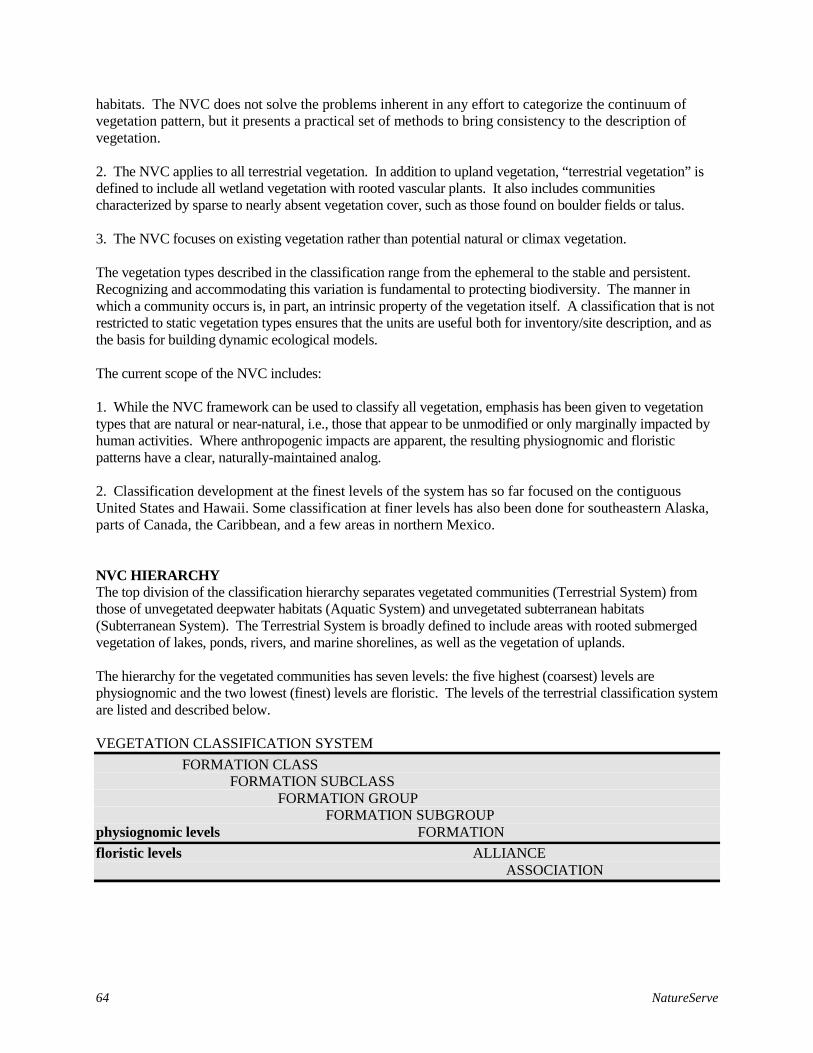
64 NatureServe
habitats. The NVC does not solve the problems inherent in any effort to categorize the continuum of vegetation pattern, but it presents a practical set of methods to bring consistency to the description of vegetation. 2. The NVC applies to all terrestrial vegetation. In addition to upland vegetation, “terrestrial vegetation” is defined to include all wetland vegetation with rooted vascular plants. It also includes communities characterized by sparse to nearly absent vegetation cover, such as those found on boulder fields or talus. 3. The NVC focuses on existing vegetation rather than potential natural or climax vegetation. The vegetation types described in the classification range from the ephemeral to the stable and persistent. Recognizing and accommodating this variation is fundamental to protecting biodiversity. The manner in which a community occurs is, in part, an intrinsic property of the vegetation itself. A classification that is not restricted to static vegetation types ensures that the units are useful both for inventory/site description, and as the basis for building dynamic ecological models. The current scope of the NVC includes: 1. While the NVC framework can be used to classify all vegetation, emphasis has been given to vegetation types that are natural or near-natural, i.e., those that appear to be unmodified or only marginally impacted by human activities. Where anthropogenic impacts are apparent, the resulting physiognomic and floristic patterns have a clear, naturally-maintained analog. 2. Classification development at the finest levels of the system has so far focused on the contiguous United States and Hawaii. Some classification at finer levels has also been done for southeastern Alaska, parts of Canada, the Caribbean, and a few areas in northern Mexico. NVC HIERARCHY The top division of the classification hierarchy separates vegetated communities (Terrestrial System) from those of unvegetated deepwater habitats (Aquatic System) and unvegetated subterranean habitats (Subterranean System). The Terrestrial System is broadly defined to include areas with rooted submerged vegetation of lakes, ponds, rivers, and marine shorelines, as well as the vegetation of uplands. The hierarchy for the vegetated communities has seven levels: the five highest (coarsest) levels are physiognomic and the two lowest (finest) levels are floristic. The levels of the terrestrial classification system are listed and described below. VEGETATION CLASSIFICATION SYSTEM
FORMATION CLASS FORMATION SUBCLASS FORMATION GROUP FORMATION SUBGROUP physiognomic levels FORMATION
floristic levels ALLIANCE ASSOCIATION
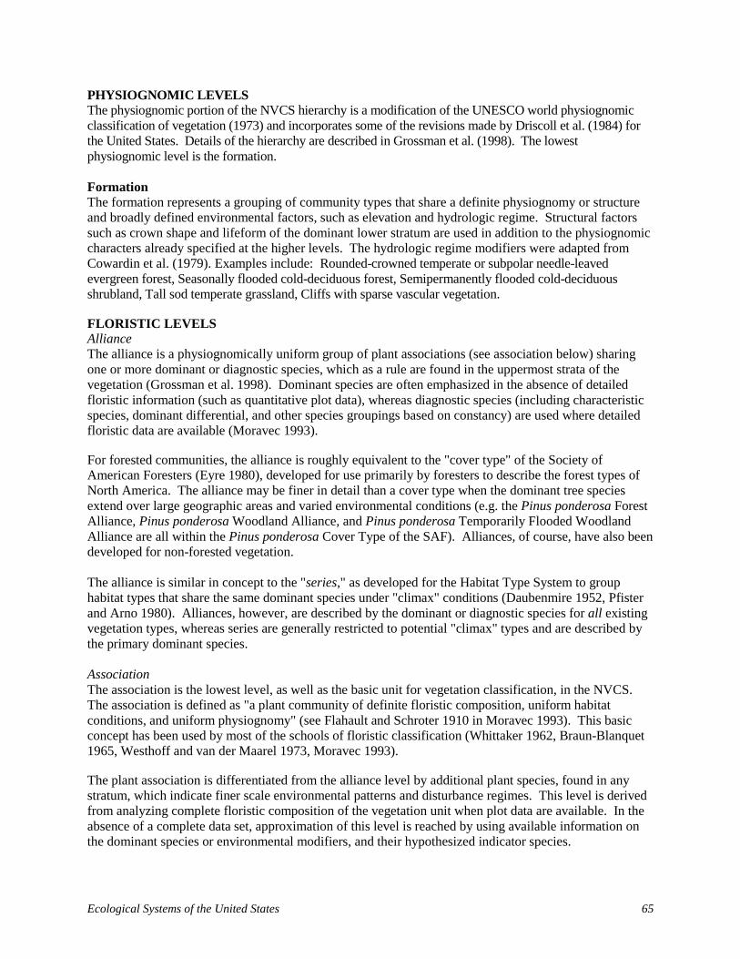
Ecological Systems of the United States 65
PHYSIOGNOMIC LEVELS The physiognomic portion of the NVCS hierarchy is a modification of the UNESCO world physiognomic classification of vegetation (1973) and incorporates some of the revisions made by Driscoll et al. (1984) for the United States. Details of the hierarchy are described in Grossman et al. (1998). The lowest physiognomic level is the formation. Formation The formation represents a grouping of community types that share a definite physiognomy or structure and broadly defined environmental factors, such as elevation and hydrologic regime. Structural factors such as crown shape and lifeform of the dominant lower stratum are used in addition to the physiognomic characters already specified at the higher levels. The hydrologic regime modifiers were adapted from Cowardin et al. (1979). Examples include: Rounded-crowned temperate or subpolar needle-leaved evergreen forest, Seasonally flooded cold-deciduous forest, Semipermanently flooded cold-deciduous shrubland, Tall sod temperate grassland, Cliffs with sparse vascular vegetation. FLORISTIC LEVELS Alliance The alliance is a physiognomically uniform group of plant associations (see association below) sharing one or more dominant or diagnostic species, which as a rule are found in the uppermost strata of the vegetation (Grossman et al. 1998). Dominant species are often emphasized in the absence of detailed floristic information (such as quantitative plot data), whereas diagnostic species (including characteristic species, dominant differential, and other species groupings based on constancy) are used where detailed floristic data are available (Moravec 1993). For forested communities, the alliance is roughly equivalent to the "cover type" of the Society of American Foresters (Eyre 1980), developed for use primarily by foresters to describe the forest types of North America. The alliance may be finer in detail than a cover type when the dominant tree species extend over large geographic areas and varied environmental conditions (e.g. the Pinus ponderosa Forest Alliance, Pinus ponderosa Woodland Alliance, and Pinus ponderosa Temporarily Flooded Woodland Alliance are all within the Pinus ponderosa Cover Type of the SAF). Alliances, of course, have also been developed for non-forested vegetation. The alliance is similar in concept to the "series," as developed for the Habitat Type System to group habitat types that share the same dominant species under "climax" conditions (Daubenmire 1952, Pfister and Arno 1980). Alliances, however, are described by the dominant or diagnostic species for all existing vegetation types, whereas series are generally restricted to potential "climax" types and are described by the primary dominant species. Association The association is the lowest level, as well as the basic unit for vegetation classification, in the NVCS. The association is defined as "a plant community of definite floristic composition, uniform habitat conditions, and uniform physiognomy" (see Flahault and Schroter 1910 in Moravec 1993). This basic concept has been used by most of the schools of floristic classification (Whittaker 1962, Braun-Blanquet 1965, Westhoff and van der Maarel 1973, Moravec 1993). The plant association is differentiated from the alliance level by additional plant species, found in any stratum, which indicate finer scale environmental patterns and disturbance regimes. This level is derived from analyzing complete floristic composition of the vegetation unit when plot data are available. In the absence of a complete data set, approximation of this level is reached by using available information on the dominant species or environmental modifiers, and their hypothesized indicator species.

66 NatureServe
Table 1.3. Three Examples from the National Vegetation Classification Hierarchy CLASS FOREST WOODLAND SHRUBLAND SUBCLASS Deciduous Forest Evergreen Woodland Deciduous Shrubland GROUP Cold-deciduous Forest Temperate or Subpolar Needle-leaved
Evergreen Woodland Temperate Broad-leaved Evergreen Shrubland
SUBGROUP Natural/Semi-natural Natural/Semi-natural Natural/Semi-natural FORMATION Lowland or Submontane Cold-
deciduous Forest Saturated Temperate or Subpolar Needle-leaved Evergreen Woodland
Sclerophyllous Temperate Broad-leaved Evergreen Shrubland
ALLIANCE Quercus stellata - Quercus marilandica Forest Alliance
Pinus palustris Saturated Woodland Alliance
Quercus havardii Shrubland Alliance
ASSOCIATION Quercus stellata - Quercus marilandica - Carya (glabra, texana) / Vaccinium arboreum Forest
Pinus palustris / Leiophyllum buxifolium / Aristida stricta Woodland
Quercus havardii - (Penstemon ambiguus, Croton dioicus) / Sporobolus giganteus Shrubland

Ecological Systems of the United States 67
Appendix 2. Element Occurrence Specifications Elements, the basic components of biodiversity tracked by NatureServe and its natural heritage program members, include species, communities, and ecosystems. Element Occurrence Specifications provide the methodology for deciding when two or more mapped polygons of an element represent a single occurrence) (see Stein and Davis 2000). Methods previously developed for community occurrences apply with limited modification to ecological systems (NatureServe 2003).
General Guidelines
Minimum criteria. For communities and systems, minimum criteria for EOs are implicit in the classification of the Element. A brief description of the Element (e.g., composition, structure, ecological processes, component associations) that includes information on characteristics that distinguish it from similar communities or systems should be provided in a global Element summary field. Any area that is large enough to be classified as a particular community or system Element has, in essence, met the minimum criteria for an occurrence of that type. Practically, however, minimum sizes may be helpful and should be provided in the EO specifications. Note that the minimum EO requirement is not based on the C/D threshold. Otherwise, all D-ranked EOs are, by definition, not EOs. Thus a System label could be applied to a small 10 ha stand of Shortleaf Pine-Hardwood Matrix System in an agricultural landscape. It may not be viable, and it may be that Network ecologists would not document the EO (unless it was a very rare community or system), but it could still be an EO. It is important to distinguish issues of EO-Tracking versus minimum EO specs. The minimum size is the smallest size of a component "core association" or cluster of associations that is recognizable (classifiable) as a System Element. Recommended minimum sizes for the different community pattern types are: 2 hectares for matrix; 0.4 hectare for large patch; 0.05 hectare for small patch; and 30 meters in length for linear. Recommended minimum sizes for the system types will meet or exceed those of the component community types. They are: 10 ha for matrix, 10 ha for upland large patch; 1 ha for wetland large patch; 0.5 ha for small patch; 100 m for all linear types. Stands/areas below the recommended minimum size become difficult to judge in terms of community or system type characteristics, and, if isolated, become heavily influenced by edge effects. For conservation purposes, generally only larger sized occurrences of each community type are tracked and the threshold for minimum size is seldom approached.
Separating EOs: Principal EOs are typically separated from other principal EOs, either by barriers or breaks, or by specified distances across intervening areas. For communities or systems, separation distances will be measured across intervening areas of different natural or semi-natural communities, or cultural vegetation based on their effect on ecological processes or species interactions.

68 NatureServe
Barriers Known barriers for Elements, either naturally occurring or manmade, should be described in the EO specifications. For community or system EOs, barriers may be obstacles that limit the expansion or alter the function of these types. These barriers either separate populations of most of the component species within the community or system, thus obstructing or severely limiting gene flow and ecological interactions or they obstruct or limit ecological processes that these species depend on. Barriers may be common for many aquatic and wetland communities or systems, but are typically less common for many upland terrestrial communities or systems.
Separation Distances In addition to barriers that totally, or almost completely, prevent ecological processes and species interactions, there may be habitats between two stands of an element that partially restrict species interactions or ecological processes. Unlike barriers, their effect depends on the kind and extent of this intervening habitat and its effect on the stands. This leads to the issue of separation distance. The intent of assigning values for separation distances between two stands is to achieve consistency in the manner in which EOs are defined and mapped. Thus, smaller separation distances are used when the intervening habitat is highly restrictive to the ecological processes or species interactions the element depends, and greater distances are used when these habitats are less prohibitive to ecological processes or species interactions. We use two broad categories of intervening habitats to define separation distances, namely – natural/semi-natural vegetation or cultural vegetation. Generally speaking, intervening natural and semi-natural vegetation will have less of an ecological effect between two stands of an EO than intervening cultural vegetation. Thus rather simplistically, we suggest that different separation distances be specified for these two kinds of situations. Typically, a shorter separation distance is specified when the intervening habitat is cultural vegetation than when it is natural/semi-natural. Minimum values for separation distances have been recommended to ensure that EOs are not separated by unreasonably small distances, which would lead to the identification of unnecessarily splintered stands as potential targets for conservation planning or action. For communities or systems, the minimum separation distance for intervening areas of different natural or semi-natural communities is set at 1 km or greater, and for intervening areas of cultural vegetation, the distance is set at 0.5 km or greater.4 Table 2.1 summarizes the recommended minimum separation distances for community and system EOs. These separation distances may, of course, be much larger. For communities or systems found primarily in mountainous regions, where habitat tends to be less fragmented, separation distances may be 5 km or more. It is possible that these separation distances could be further refined by considering the kind of natural/semi-natural or cultural vegetation present. Intervening natural and semi-natural areas with similar kinds of habitat characteristics to the stands of a community or system under consideration will have less of an effect on community or system processes than those with very different kinds of characteristics. For example, bog stands separated by intervening areas of upland jack pine on bedrock could be more readily treated as distinct EOs than bogs separated by areas of black spruce swamp. However, at this time, no specific guidelines are suggested for these situations, but if used, they should be documented.
4 Minimum distances for systems are no less than, and may exceed, that of communities. Further review of their recommendations are needed.

Ecological Systems of the United States 69
Table 2.1 - Recommended Minimum Separation Distances for
Communities and Ecological Systems
Type of Separation Minimum Separation Distance
Barrier qualitatively defined
cultural vegetation ≥ 0.5 km
different natural or semi-natural communities or systems
≥ 1 km
Example
ELEMENT North-Central Interior Dry-Mesic Oak Forest and Woodland System (CES202.046) SPECS GROUP None MINIMUM CRITERIA This system is found throughout the glaciated regions of the Midwest, typically in gently rolling landscapes. It can occur on uplands within the prairie matrix and near floodplains, or on rolling glacial moraines and among kettle-kame topography. Soils are typically well-drained Mollisols or Alfisols that range from loamy to sandy loam in texture. Historically, this type was quite extensive in MI, IN, IL, MO, IA, WI, and MN. Well over 700,000 hectares likely occurred in southern Michigan alone circa 1800. It is distinct from other forested systems within the region by a dry-mesic edaphic condition that is transitional between dry oak forests and woodlands and mesic hardwood forests, such as maple-basswood forests. Forest cover can range from dense to moderately open canopy and there is commonly a dense shrub layer. Fire-resistant oak species, in particular Quercus macrocarpa, Q. rubra, and/or Q. alba dominate the overstory. Carya spp., including C. ovata, C. cordiformis, and C. tomentosa are diagnostic in portions of the range of this system. Depending on range of distribution, and overstory canopy density, the understory may include species such as Corylus americana, Amelanchier spp., Maianthemum stellatum, Caulophyllum thalictroides, Laportea canadensis, Trillium grandiflorum, Aralia nudicaulis, and Urtica dioica. Occasionally, prairie grasses such as Andropogon gerardii and Panicum virgatum may be present. Fire constitutes the main natural process for this type and likely maintained a more open canopy structure to support oak regeneration. Historic fire frequency was likely highest in the prairie-forest border areas. Fire suppression may account for the more closed oak forest examples of this system with the more mesic understory. It likely has allowed for other associates such as Acer saccharum, Celtis occidentalis, Liriodendron tulipifera, Ostrya virginiana, and Juglans nigra to become more prevalent, especially in upland areas along floodplains. Extensive conversion for agriculture has fragmented these systems. Continued fire suppression has also resulted in succession to mesic hardwoods, such that in many locations, no oak species are regenerating. Remaining large areas of this system are likely under considerable pressure due to conversion to agriculture, pastureland, and urban development. Minimum Size: 10 ha

70 NatureServe
EO Separation SEPARATION BARRIERS Barriers that would separate patches of this community include a four-lane highway, urban development, and an open body of water or large river. The open bodies of water or river may act as a fire-break. SEPARATION DISTANCE – NATURAL/SEMI-NATURAL VEGETATION 4 km SEPARATION DISTANCE – CULTURAL VEGETATION 0.5 km ALTERNATE SEPARATION PROCEDURE SEPARATION JUSTIFICATION The separation factors for natural/semi-natural vegetation reflect the relatively ease with which species and processes move between systems in the relatively flat glaciated landscape. In addition, seed dispersal of Quercus and Carya spp., which are dependent on squirrels and jays. These dispersers can move considerable distances between patches in intact or fragmented landscapes, from several hundred meters to 4 or 5 km (Harrison and Werner 1984, Crow 1988, Johnson and Webb 1989). Separation distance for cultural vegetation is set at minimum default value. FEATURE LABELS GSPECS AUTHORSHIP D. Faber-Langendoen GSPECS DATE 2003-04-02 GSPECS NOTES
Distinctions within Element Occurrences.
Although the EO conceptually represents the entire occupied area, there may be smaller geographically distinct areas within the principal EO for which information could be useful for conservation planning, biological monitoring, or biological management at local levels. These geographically nested components are referred to as sub-EOs, and the main EO is referred to as the Principal EO. Sub-EOs must be contained within a principal EO of the same Element. Note that sub-EOs should not be created simply to represent different parts of a principal EO comprised of noncontiguous patches.
Sub-EOs may be defined as
a) areas of differing composition, or higher density, quality, or conservation concern (e.g., different age stands or successional phases, old growth patches);
b) discrete areas for which it is desirable to maintain information for each area in separate records (e.g., to facilitate recording of monitoring data); or
c) other areas marked by non-biological divisions assigned for convenience in mapping, monitoring, or management (e.g., geographic, political, and land survey map units). The creation of sub-EOs defined by these divisions should generally be avoided because they are not biologically significant.5
Sub-EOs can be used to facilitate information management in cases where a principal EO is particularly large, complex, or crosses jurisdictional boundaries. Such principal EOs may present challenges, including
5 Some geographic units, such as watersheds, may sometimes reflect biological divisions, particularly for many freshwater Elements.

Ecological Systems of the United States 71
incomplete knowledge of the full extent of the EO, loss of detail about specific sub-populations or community patches, and difficulty in supporting information needs related to inventory, monitoring, management, conservation planning, and environmental review. However, sub-EOs should not replace the use of a principal EO to represent the full extent of the occurrence.
Community-level EOs should not be treated as sub-EOs of System EOs, as they are two different classification systems, and each level can exist independent of the other (unlike the EO – sub-EO relationship). Doing so would also complicate the ability to track sub-EO features listed above at either level. However, where a community-level EO is a spatial component of a System EO, it is desirable to attribute the community EO with the System EO code in order to display their relationships.
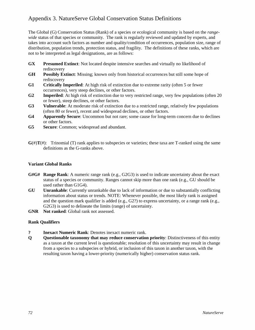
72 NatureServe
Appendix 3. NatureServe Global Conservation Status Definitions The Global (G) Conservation Status (Rank) of a species or ecological community is based on the range-wide status of that species or community. The rank is regularly reviewed and updated by experts, and takes into account such factors as number and quality/condition of occurrences, population size, range of distribution, population trends, protection status, and fragility. The definitions of these ranks, which are not to be interpreted as legal designations, are as follows: GX Presumed Extinct: Not located despite intensive searches and virtually no likelihood of
rediscovery GH Possibly Extinct: Missing; known only from historical occurrences but still some hope of
rediscovery G1 Critically Imperiled: At high risk of extinction due to extreme rarity (often 5 or fewer
occurrences), very steep declines, or other factors. G2 Imperiled: At high risk of extinction due to very restricted range, very few populations (often 20
or fewer), steep declines, or other factors. G3 Vulnerable: At moderate risk of extinction due to a restricted range, relatively few populations
(often 80 or fewer), recent and widespread declines, or other factors. G4 Apparently Secure: Uncommon but not rare; some cause for long-term concern due to declines
or other factors. G5 Secure: Common; widespread and abundant. G(#)T(#): Trinomial (T) rank applies to subspecies or varieties; these taxa are T-ranked using the same
definitions as the G-ranks above. Variant Global Ranks G#G# Range Rank: A numeric range rank (e.g., G2G3) is used to indicate uncertainty about the exact
status of a species or community. Ranges cannot skip more than one rank (e.g., GU should be used rather than G1G4).
GU Unrankable: Currently unrankable due to lack of information or due to substantially conflicting information about status or trends. NOTE: Whenever possible, the most likely rank is assigned and the question mark qualifier is added (e.g., G2?) to express uncertainty, or a range rank (e.g., G2G3) is used to delineate the limits (range) of uncertainty.
GNR Not ranked: Global rank not assessed. Rank Qualifiers ? Inexact Numeric Rank: Denotes inexact numeric rank. Q Questionable taxonomy that may reduce conservation priority: Distinctiveness of this entity
as a taxon at the current level is questionable; resolution of this uncertainty may result in change from a species to a subspecies or hybrid, or inclusion of this taxon in another taxon, with the resulting taxon having a lower-priority (numerically higher) conservation status rank.

Ecological Systems of the United States 73
Appendix 4. Terrestrial Ecological Systems and Wildlife Habitats in California
System Code Terrestrial Ecological System Name California WHR Classes
Mainly Wetland
CES302.759 Sonoran Fan Palm Oasis Palm oasis
CES304.780 Inter-Mountain Basins Greasewood Flat Desert riparian
CES206.944
Mediterranean California Foothill and Lower Montane Riparian Woodland
Montane riparian/Valley foothill riparian
CES206.945
Mediterranean California Serpentine Foothill and Lower Montane Riparian Woodland and Seeps Montane riparian
CES206.946 California Central Valley Riparian Woodland and Shrubland Valley foothill riparian/Valley oak
woodland
CES300.729 North American Arid West Emergent Marsh Freshwater emergent wetland
CES302.747 North American Warm Desert Cienega Freshwater emergent wetland
CES302.748
North American Warm Desert Lower Montane Riparian Woodland and Shrubland Montane riparian
CES302.752 North American Warm Desert Riparian Mesquite Bosque Desert riparian
CES302.753 North American Warm Desert Riparian Woodland and Shrubland Desert riparian
CES302.755 North American Warm Desert Wash Desert dry wash CES304.768 Columbia Basin Foothill Riparian Woodland and Shrubland Montane riparian
CES200.876 Temperate Pacific Freshwater Aquatic Bed Freshwater emergent wetland
CES200.877 Temperate Pacific Freshwater Emergent Marsh Freshwater emergent wetland
CES204.880 North Pacific Maritime Tidal Salt Marsh Saline emergent marsh
CES206.947 Mediterranean California Alkali Marsh Freshwater emergent wetland
CES206.948 Northern California Claypan Vernal Pool Annual grassland
CES206.949 Northern California Volcanic Vernal Pool Annual grassland
CES206.950 South Coastal California Vernal Pools Annual grassland
CES206.951 Mediterranean California Coastal Interdunal Wetland Freshwater emergent wetland
CES206.952 Mediterranean California Subalpine-Montane Fen Freshwater emergent wetland
CES206.953 Mediterranean California Serpentine Fen Freshwater emergent wetland
CES206.954 California Central Valley Alkali Sink Freshwater emergent wetland
CES204.996 Modoc Basalt Flow Vernal Pools Annual grassland
CES200.997 Temperate Pacific Brackish Marsh Estuarine
CES200.998 Temperate Pacific Montane Wet Meadow Wet Meadow
CES206.999 Mediterranean California Eel Grass Beds Marine
CES206.002 Mediterranean California Coastal Salt Marsh Saline emergent marsh
CES304.045
Great Basin Foothill and Lower Montane Riparian Woodland and Shrubland Montane riparian
CES302.751 North American Warm Desert Playa Alkali desert scrub
CES304.781 Inter-Mountain Basins Greasewood Wash Desert dry wash
CES304.786 Inter-Mountain Basins Playa Alkali desert scrub
CES200.878 Temperate Pacific Freshwater Mudflat
Mainly Upland
CES302.741 Mogollon Chaparral Mixed chaparral
CES302.742 Mojave Mid-Elevation Mixed Desert Scrub Joshua tree
CES302.749 Sonora-Mojave Desert Mixed Salt Desert Scrub Alkali desert scrub CES302.756 Sonora-Mojave Creosotebush-White Bursage Desert Scrub Desert scrub

74 NatureServe
System Code Terrestrial Ecological System Name California WHR Classes
CES302.757 Sonora-Mojave-Baja Semi-Desert Chaparral Mixed chaparral
CES302.760 Sonoran Granite Outcrop Desert Scrub Desert scrub
CES302.761 Sonoran Paloverde-Mixed Cacti Desert Scrub Desert succulent scrub
CES304.769 Columbia Plateau Western Juniper Savanna Juniper
CES304.772 Inter-Mountain Basins Mountain Mahogany Woodland and Shrubland
CES304.773 Great Basin Pinyon-Juniper Woodland Pinyon-juniper
CES304.774 Great Basin Xeric Mixed Sagebrush Shrubland Sagebrush
CES304.777 Inter-Mountain Basins Big Sagebrush Shrubland Sagebrush
CES304.778 Inter-Mountain Basins Big Sagebrush Steppe Sagebrush
CES304.782 Inter-Mountain Basins Juniper Savanna Juniper
CES304.784 Inter-Mountain Basins Mixed Salt Desert Scrub Alkali desert scrub
CES304.785 Inter-Mountain Basins Montane Sagebrush Steppe Sagebrush
CES304.787 Inter-Mountain Basins Semi-Desert Grassland Perennial grassland
CES304.788 Inter-Mountain Basins Semi-Desert Shrub Steppe Perennial grassland
CES304.789 Inter-Mountain Basins Shale Badland Alkali desert scrub CES304.790 Inter-Mountain Basins Subalpine Limber-Bristlecone Pine Woodland Subalpine conifer
CES306.813 Rocky Mountain Aspen Forest and Woodland Aspen
CES204.852 North Pacific Oak Woodland Montane hardwood
CES206.900 Mediterranean California Alpine Fell-Field Low sagebrush
CES206.909 Mediterranean California Mixed Oak Woodland Montane hardwood
CES206.910 Mediterranean California Subalpine Woodland Subalpine conifer
CES206.911 Northern Pacific Mesic Subalpine Woodland Subalpine conifer
CES206.912 Sierra Nevada Subalpine Lodgepole Pine Forest and Woodland Lodgepole pine
CES206.913 Mediterranean California Red Fir Forest and Woodland Red fir
CES206.914
Klamath-Siskyou Upper Montane Serpentine Mixed Conifer Woodland Klamath mixed conifer
CES206.915 Mediterranean California Mesic Mixed Conifer Forest and Woodland Sierran mixed conifer forest/White
fir/Douglas fir
CES206.916
Mediterranean California Dry-Mesic Mixed Conifer Forest and Woodland
Sierran mixed conifer forest/White fir/Douglas fir
CES206.917
Klamath-Siskyou Lower Montane Serpentine Mixed Conifer Woodland Klamath mixed conifer
CES206.918
Mediterranean California Ponderosa-Jeffrey Pine Forest and Woodland
Ponderosa pine/Jeffrey pine/Eastside pine
CES206.919 Northern California Mixed Evergreen Forest Montane hardwood/Douglas fir
CES206.920 Central and Southern California Mixed Evergreen Woodland Montane hardwood
CES206.921 Coastal Redwood-Mixed Conifer Forest and Woodland Redwood/Douglas fir
CES206.922 Coastal Closed-Cone Conifer Forest and Woodland Closed-cone pine-cypress
CES206.923 Mediterranean California Mixed Oak-Evergreen Woodland Montane hardwood - conifer
CES206.924 Sierra Nevada Alpine Dwarf Shrubland Alpine dwarf shrub/Low sagebrush
CES206.925 California Montane Woodland and Chaparral Montane chaparral
CES206.926 California Mesic Chaparral Mixed chaparral
CES206.927 California Xeric Serpentine Chaparral Mixed chaparral
CES206.928 Mesic Serpentine Woodland and Chaparral Mixed chaparral
CES206.929 California Maritime Chaparral Mixed chaparral
CES206.930 Southern California Dry-Mesic Chaparral Chamise-red shank

Ecological Systems of the United States 75
System Code Terrestrial Ecological System Name California WHR Classes
CES206.931 Northern and Central California Dry-Mesic Chaparral Mixed chaparral
CES206.932 Northern California Coastal Scrub Coastal scrub
CES206.933 Southern California Coastal Scrub Coastal scrub
CES206.934 Baja Semi-Desert Coastal Succulent Scrub Desert succulent scrub
CES206.935 California Central Valley Mixed Oak Savanna Blue oak woodland/Valley oak
woodland
CES206.936 California Lower Montane Pine-Oak Woodland and Savanna Blue oak-Digger pine
CES206.937 California Coastal Live Oak Woodland and Savanna Coastal oak woodland
CES206.938 Southern California Oak Woodland and Savanna Coastal oak woodland
CES206.939 Mediterranean California Alpine Dry Tundra Perennial grassland
CES206.940 Mediterranean California Subalpine Meadow Perennial grassland
CES206.941 California Northern Coastal Grassland Perennial grassland
CES206.942 California Central Valley and Southern Coastal Grassland Perennial grassland
CES206.943 California Mesic Serpentine Grassland Perennial grassland
CES204.100 North Pacific Montane Grassland Perennial grassland
CES304.001 Great Basin Semi-Desert Chaparral Mixed chaparral
CES304.042 Great Basin Altered Andesite Pine Woodland Ponderosa pine/Jeffery pine Mainly Sparsely Vegetated
CES302.744 North American Warm Desert Active and Stabilized Dunes Desert scrub
CES302.745 North American Warm Desert Bedrock Cliff and Outcrop
CES302.750 North American Warm Desert Pavement
CES302.754 North American Warm Desert Volcanic Rockland
CES304.779 Inter-Mountain Basins Cliff and Canyon
CES206.899 Mediterranean California Alpine Bedrock and Scree
CES206.901 Sierra Nevada Cliff and Canyon
CES206.902 Klamath-Siskyou Cliff and Outcrop
CES206.903 Central California Coast Ranges Cliff and Canyon
CES206.904 Southern California Coast Ranges Cliff and Canyon
CES206.905 Mediterranean California Serpentine Barrens
CES206.906 Mediterranean California Coastal Bluff Coastal scrub (in part)
CES206.907 Mediterranean California Northern Coastal Dunes Coastal scrub (in part)
CES206.908 Mediterranean California Southern Coastal Dunes Coastal scrub (in part)

Field Key to the Ecological Systems and Habitat Systems
of the Northeastern United States
Susan C. Gawler
Regional Vegetation Ecologist
NatureServe
Boston, Massachusetts
December 2008

NY
PA
VA
ME
WV
VT
NH
MD
NJ
MA
CT
DE
RI
DC
Cover photos:
top: Acadian-Appalachian Subalpine Woodland and Heath-Krummholz system (Alpine Macrogroup),
Borestone Mountain, Maine. photo © Susan C. Gawler
middle: Central and Southern Appalachian Montane Oak Forest (Central Oak-Pine macrogroup),
George Washington and Jefferson National Forest, Virginia. photo © Gary P. Fleming
bottom: Central Appalachian River Floodplain system (Northeastern Floodplain Forest macrogroup),
Potomac River along the Chesapeake and Ohio Canal National Historical Park, Maryland (looking across to
Virginia). photo © Susan C. Gawler
This work was supported by various grants involving ecological systems and habitats. We are
grateful for funding from LANDFIRE, USGS Gap Analysis Program, the National Park Service,
the National Fish and Wildlife Foundation, and the Northeast Association of Fish and Wildlife
Agencies.
Comments and suggestions can be sent to the author via email: [email protected].

Field Key to the Ecological Systems and Habitat Systems
of the Northeastern United States
Contents
Introduction ................................................................................................................................... 1
Table 1. Macrogroups used to organize northeastern ecological systems. .......................... 2
Table 2. Altered Vegetation and Developed Classes not included in the keys .................. 7
Keys to Ecological Systems of the Northeastern United States ................................................... 9
Key to the Major Divisions of the Key ..................................................................................... 9
KEY A – UPLAND FORESTS, WOODLANDS, AND GLADES ....................................... 10
KEY B – WETLAND FORESTS & WOODLANDS ............................................................ 22
KEY C – HERB/SHRUB AND SPARSELY VEGETATED UPLANDS ............................ 28
KEY D – HERBACEOUS AND HERB/SHRUB WETLANDS .......................................... 36
Literature Cited ........................................................................................................................... 41
Appendix A: Cross-reference to plant common names and scientific names. ........................... 42
Appendix B: USNVC organizing hierarchy, Formation to Macrogroup ................................... 52


1
Introduction
The following keys to ecological systems and other habitats cover the northeastern states of Maine,
New Hampshire, Vermont, New York, Massachusetts, Rhode Island, Connecticut, New Jersey,
Pennsylvania, Delaware, Maryland, Virginia, and West Virginia, as well as the District of
Columbia. They were developed as a general regional tool, as well as with the specific purpose of
supporting the mapping and application phases of the Northeast Terrestrial Habitat Classification
System (NETHCS). The NETHCS, which these keys cover, is the foundation of the habitat
systems map currently being developed for the Northeast Association of Fish & Wildlife Agencies
(NEAFWA) (Gawler 2008). The keys include wide-ranging habitats as well as types that
characteristically occur in small patches and hence may not be mappable at the scale used in the
northeast habitat map. We have chosen to be inclusive so that the user will have information on all
system types for comparison purposes. This document is intended as an evolving tool and may be
updated as experience and additional information dictate.
The NETHCS was developed as a comprehensive and standardized representation of habitats for
wildlife that would be consistent with other regional classification and mapping efforts. It is based
on the ecological systems classification created by NatureServe, with additional classes for
developed and highly altered lands. These Habitat Systems are intended to be applicable at
medium and large scales, and to supplement finer-scale approaches used within states for specific
habitat conservation projects, whether for particular animal or plant species, or landscape-level
approaches. They include types that cover extensive areas, as well as small, specific-environment
types that may cover only a hectare or two. In the Northeast, all ecological systems (sensu Comer
et al. 2003) can also be considered habitat system (sensu Gawler 2008), and the habitat systems
additionally include altered and developed classes. For information on the development of the
NETHCS and its structure, refer to the classification report (Gawler et al. 2008), available at
http://www.rcngrants.org/node/38. For background on NatureServe‟s ecological systems, refer to
Comer et al. 2003, available at http://www.natureserve.org/publications/usEcologicalsystems.jsp.
Ecological systems are vegetation-based because plants are sedentary and integrate the effects of
environment in a way that reflects important habitat values. The keys use dominant or
characteristic trees, shrubs, and (where needed) herbs for diagnostic characters. Common names
are generally used, with the scientific name following the nomenclature of Kartesz (1999) given
the first time a plant species is referred to in the key. The Appendix provides a cross-reference
between common and scientific names.
The habitat systems in the Northeast Terrestrial Habitat Classification are organized into the
Macrogroup level of the US National Vegetation Classification (FGDC 2008), providing
flexibility in applying the classification. Systems are not part of the USNVC hierarchy per se,
but we have found the macrogroup level of the USNVC to be a convenient organizing tool. The
143 Habitat Systems are grouped into 35 macrogroups (Table 1), with each system linked to the
macrogroup with which it bears overall closest similarity. Macrogroups are aggregated into
broad Formation Classes. Bear in mind, however, that a particular system does not always nest
neatly within one macrogroup. The keys go first to Macrogroup and, within each macrogroup, a
subordinate key goes to ecological systems. For this regional approach, macrogroup names have
been simplified from those in the USNVC; a complete treatment is given in Appendix B.

2
Table 1. Macrogroups used to organize northeastern ecological systems.
See Appendix B for further detail. FORMATION CLASS 1. FOREST AND WOODLAND
Longleaf Pine
Southern Oak-Pine
Central Oak-Pine
Northern Hardwood & Conifer
Plantation and Ruderal Forest
Exotic Upland Forest
Southern Bottomland Forest
Coastal Plain Swamp
Central Hardwood Swamp
Northeastern Floodplain Forest
Northern Swamp
Boreal Upland Forest
Boreal Forested Peatland
FORMATION CLASS 2. SHRUBLAND AND GRASSLAND
Glade and Savanna
Outcrop/Summit Scrub
Lake & River Shore
Ruderal Shrubland & Grassland
Coastal Grassland & Shrubland
Northern Peatland
Coastal Plain Peatland
Central Appalachian Peatland
Coastal Plain Pond
Emergent Marsh
Wet Meadow / Shrub Marsh
Modified/Managed Wetland
Salt Marsh
FORMATION CLASS 4. POLAR AND HIGH MONTANE
Alpine
FORMATION CLASS 5. AQUATIC
Intertidal Shore
FORMATION CLASS 6. SPARSELY VEGETATED ROCK
Cliff and Talus
Flatrock
Rocky Coast
FORMATION CLASS 7. AGRICULTURAL
Agricultural
FORMATION CLASS 8. DEVELOPED
Maintained Grasses and Mixed Cover
Urban/Suburban Built
Extractive
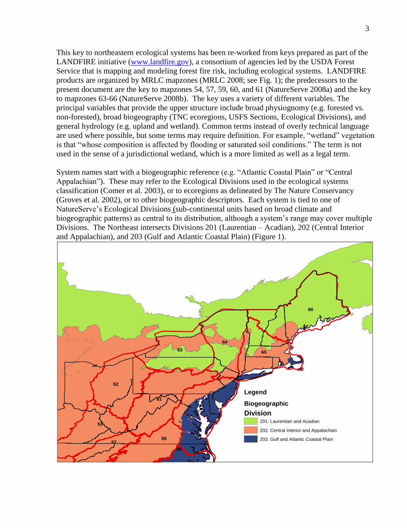
3
This key to northeastern ecological systems has been re-worked from keys prepared as part of the
LANDFIRE initiative (www.landfire.gov), a consortium of agencies led by the USDA Forest
Service that is mapping and modeling forest fire risk, including ecological systems. LANDFIRE
products are organized by MRLC mapzones (MRLC 2008; see Fig. 1); the predecessors to the
present document are the key to mapzones 54, 57, 59, 60, and 61 (NatureServe 2008a) and the key
to mapzones 63-66 (NatureServe 2008b). The key uses a variety of different variables. The
principal variables that provide the upper structure include broad physiognomy (e.g. forested vs.
non-forested), broad biogeography (TNC ecoregions, USFS Sections, Ecological Divisions), and
general hydrology (e.g. upland and wetland). Common terms instead of overly technical language
are used where possible, but some terms may require definition. For example, “wetland” vegetation
is that “whose composition is affected by flooding or saturated soil conditions.” The term is not
used in the sense of a jurisdictional wetland, which is a more limited as well as a legal term.
System names start with a biogeographic reference (e.g. “Atlantic Coastal Plain” or “Central
Appalachian”). These may refer to the Ecological Divisions used in the ecological systems
classification (Comer et al. 2003), or to ecoregions as delineated by The Nature Conservancy
(Groves et al. 2002), or to other biogeographic descriptors. Each system is tied to one of
NatureServe‟s Ecological Divisions (sub-continental units based on broad climate and
biogeographic patterns) as central to its distribution, although a system‟s range may cover multiple
Divisions. The Northeast intersects Divisions 201 (Laurentian – Acadian), 202 (Central Interior
and Appalachian), and 203 (Gulf and Atlantic Coastal Plain) (Figure 1).
Legend
Biogeographic
Division 201. Laurentian and Acadian
202. Central Interior and Appalachian
203. Gulf and Atlantic Coastal Plain
66
61
60
62
63 65
64
53
59 57
58

4
Figure 1. Biogeographic divisions used to characterize ecological system affinities. Colors are the
Divisions; red lines outline the mapzones used in the NLCD (with their numbers).
Ideally, the users of the key will also be able to locate themselves in relation to The Nature
Conservancy ecoregions (Figure 2) or the US Forest Service ECOMAP Sections (or, in a few
cases, subsections) (Figure 3). EPA Level III Ecoregions have been used in other similar keys, but
because they are not complete to Level IV for the Northeast, we have not used them in this key. In
some cases, an ecoregion, section, or division line may be the determining factor between two
otherwise similar systems. Given the continuous nature of ecological variation, however,
transitional areas may occur near an ecoregional boundary, so the lines should be considered as
general guides.
Figure 2. TNC Ecoregions of the Northeast. The keys use the ecoregion name followed by the number in
parentheses.

5
Further details on TNC ecoregions, USFS ECOMAP Sections and subsections, and Ecological
Divisions can be found via http://www.natureserve.org/explorer/eodist.htm. Information about
regional, state, and multi-state EPA Ecoregion products can be obtained at
http://www.epa.gov/wed/pages/ecoregions/level_iv.htm. Information on the National Landcover
Database (NLCD) and the mapzones into which those products are organized, can be found at
http://www.mrlc.gov/nlcd.php.
Legend
USFS_Province_2005_EUS
PROVINCE_N
Adirondack-New England Mixed Forest--Coniferous Forest--Alpine Meadow
Central Appalachian Broadleaf Forest-Coniferous Forest-Meadow
East Laurentian Mixed Forest
Eastern Broadleaf Forest (Oceanic)
Midwest Broadleaf Forest
Outer Coastal Plain Mixed Forest
Southeastern Mixed Forest
231I
221E
221A
M221A
211F
M211A
222I
221F
232H
221D
M221D
M221B
M211D
211G
232A
M221C
211E211D
211B
M211B
232H
211I
211J
211A
221J
232I
221B
M211C
211C
221A
Figure 3. US Forest Service Sections of the Northeast (blue lines) and their numbers. Higher-level
groupings are the shaded Provinces.
The keys primarily address ecological systems (Comer et al. 2003) that represent natural or near-
natural conditions. Much of the landscape, however, has been highly altered. Many of the
NETHCS units for land-use types (e.g. developed lands) and altered vegetation are not formally
incorporated into the keys, since they are typically recognizable without the use of a key, or else
their floristic composition is so variable as to be not useful in a field key. We provide a table
below showing the NETHCS habitat systems that represent non-natural vegetation or developed

6
lands, with a short description for each. Semi-natural forests (e.g. early successional forests) and
reverting fields are included in the keys.

7
Table 2. Altered Vegetation and Developed Classes not included in the keys
Legend unit ESLF Description
Open Water Open water (intertidal flats are included in the key, but not other
aquatic habitats).
Developed Generally developed lands.
Urban/Recreational Grasses
21 Managed vegetation, primarily grassland, planted in developed settings for recreation, erosion control, or aesthetic purposes. Impervious surfaces account for less than 20 percent of total cover. Examples include parks, lawns, golf courses, airport grasses, and industrial site grasses.
Residential - Rural / Sparse
21 Sparse residential areas, or housing along rural roadsides, in which impervious surfaces account for <15% of total cover (generally corresponding to lot sizes of > 1 acre); largely single family housing.
Residential - Low Intensity
22 Areas with a mixture of constructed materials and vegetation in which impervious surfaces account for 15-25% of total cover (generally corresponding to lot sizes of 1/2 - 1 acre); mostly single-family housing units.
Residential - Medium Intensity
22 Areas with a mixture of constructed materials and vegetation in which impervious surfaces account for 25-50% of total cover (generally corresponding to lot sizes of 1/4 - 1/2); mostly single-family housing units.
Residential - High Intensity
23 Includes highly developed areas where people reside in high numbers. Examples include apartment complexes, row houses and commercial/industrial. Impervious surfaces account for 80 to100% of the total cover.
Commercial/Industrial
24 Developed areas where people reside or work in high numbers. Examples include apartment complexes, row houses and commercial/industrial. Impervious surfaces account for more than 80% of the total cover.
Quarries/Pits/Stripmines
32 Surface mining operations for various materials: sand, gravel, rock, coal, etc.
Agriculture Generally developed for agricultural uses.
Pasture/Hay
82 These agriculture lands typically have perennial herbaceous cover (e.g. regularly-shaped plantings) used for livestock grazing or the production of hay. There are obvious signs of management such as fencing and/or haying that distinguish it from natural grasslands. Identified CRP (Conservation Reserve Program) lands are included in this land cover type.
Cultivated Crops
82 Land used for the production of crops, including annual-cycle crops (corn, potatoes, small grains, oilseed crops, vegetables, flowers, etc.), and more stable land cover of orchards, vineyards, nurseries, and Christmas tree farms. Plant cover is variable depending on season and type of farming.
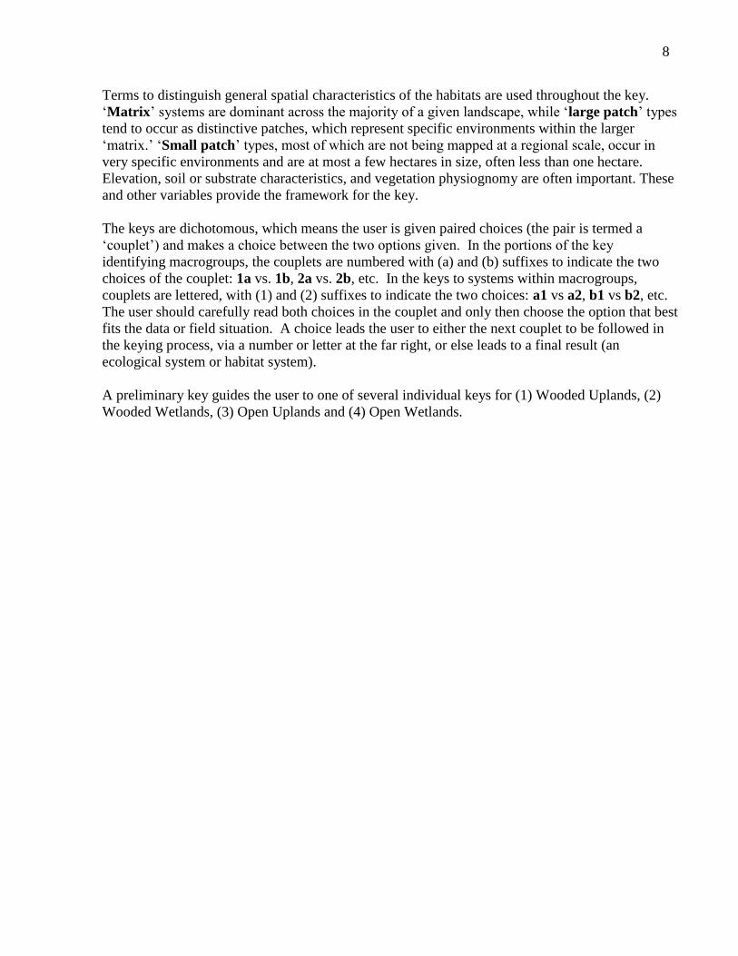
8
Terms to distinguish general spatial characteristics of the habitats are used throughout the key.
„Matrix‟ systems are dominant across the majority of a given landscape, while „large patch‟ types
tend to occur as distinctive patches, which represent specific environments within the larger
„matrix.‟ „Small patch‟ types, most of which are not being mapped at a regional scale, occur in
very specific environments and are at most a few hectares in size, often less than one hectare.
Elevation, soil or substrate characteristics, and vegetation physiognomy are often important. These
and other variables provide the framework for the key.
The keys are dichotomous, which means the user is given paired choices (the pair is termed a
„couplet‟) and makes a choice between the two options given. In the portions of the key
identifying macrogroups, the couplets are numbered with (a) and (b) suffixes to indicate the two
choices of the couplet: 1a vs. 1b, 2a vs. 2b, etc. In the keys to systems within macrogroups,
couplets are lettered, with (1) and (2) suffixes to indicate the two choices: a1 vs a2, b1 vs b2, etc.
The user should carefully read both choices in the couplet and only then choose the option that best
fits the data or field situation. A choice leads the user to either the next couplet to be followed in
the keying process, via a number or letter at the far right, or else leads to a final result (an
ecological system or habitat system).
A preliminary key guides the user to one of several individual keys for (1) Wooded Uplands, (2)
Wooded Wetlands, (3) Open Uplands and (4) Open Wetlands.
9
Keys to Ecological Systems of the Northeastern United States
Key to the Major Divisions of the Key
1a. Trees1 or tall shrubs (over 2 m) as uppermost layer, with total woody
cover in that layer 25% or more overall ................................................... 2 1b. Tree cover in the uppermost stratum less than 25% overall; uppermost
continuous vegetation stratum strongly shrubby or herbaceous2 ................. 3
2a. Upland forests, woodlands, and glades/savannas (composition is not
affected by flooding or saturated soil conditions) ...................... Key A (p. 9) 2b. Wetland or floodplain forests and woodlands (composition is affected by
flooding or saturated soil conditions; including floodplains and bottomlands as well as seepage forests) ................................. Key B (p. 21)
3a. Open uplands (e.g. grasslands and shrublands, dry summits) ..... Key C (p. 27)
3b. Open wetlands (including pond margins, marshes, shrub swamps, and wet depressions) ...................................................................... Key D (p. 35)
The key goes first to the Macrogroup level, and then for each macrogroup, a subordinate boxed key takes you to the ecological system. In the Northeast
Terrestrial Wildlife Habitat Classification system, these are the “Habitat Systems”. Common names are used for diagnostic plants, with scientific names in parentheses
the first time a particular plant is named. A cross-reference between common and scientific names (following the nomenclature of Kartesz 1999) can be found in the
Appendix. Each system’s name is followed by its ESLF number in parentheses. (ESLF numbers
are unique identifiers used in the LANDFIRE legend and adapted here.) A triple asterisk (***) after the ESLF number indicates a Small Patch ecological system or
Linear ecological system; these may not lend themselves to mapping at a regional scale, but are included for completeness of the key.
For additional information on most of these systems, those that are not highly altered or human-created, see NatureServe Explorer at
http://www.natureserve.org/explorer/servlet/NatureServe
1 Trees are defined here as woody plants >3 m tall with a single main stem.
2 Glades -- grass-dominated rocky habitats with partial tree cover (variable in amount)-- are covered in both
Key A and Key C, because of the variability in tree cover. Rocky summits have a patchwork of bare rock and
low shrub or herb cover, sometimes with scattered and often stunted trees, and are covered in the Open
Uplands key (Key C).

10
KEY A – UPLAND FORESTS, WOODLANDS, AND GLADES
1a. Forests dominated by non-native trees such as Norway maple (Acer
platanoides), tree of heaven (Ailanthus altissima), Austrian pine (Pinus nigra), or other exotics not planted as a plantation, cover of non-native
trees exceeds that of native trees; non-native plants typically frequent in the understory ............................ EXOTIC UPLAND FOREST macrogroup
One system: ......................... Introduced Upland Vegetation - Tree (8401)***
1b. Forests dominated by native trees, or forest plantations ................................ 2
2a. Plantation forests: trees apparently in rows, or other evidence of intentional planting by humans
................................. PLANTATION AND RUDERAL FOREST macrogroup
(also see couplet 7) ....................................... Managed Tree Plantation (8513)
2b. Forests and woodlands that are not planted ................................................. 3
3a. Spruce (Picea spp.) and/or fir (Abies spp.), or rarely jack pine (Pinus banksiana) as the dominant conifer trees, and conifer cover exceeding
cover of deciduous trees (except in local regenerating patches of birch (Betula spp.), red maple (Acer rubrum), etc.)
................................................. BOREAL UPLAND FOREST macrogroup3
a1. Virginia and West Virginia, usually above 900 m (3000) elevation; Fraser fir
(Abies fraseri) often present
.................. Central and Southern Appalachian Spruce-Fir Forest (4253) a2. New England and New York ...................................................................... b
b1. Forests with jack pine present, often dominant, and black spruce (Picea mariana) a frequent associate; known in the northeast only from portions of
western Maine ................... Boreal Jack Pine – Black Spruce Forest (4247) b2. Jack pine absent ...................................................................................... c
3 Habitat systems that may key here, because of inclusions of woodland cover, but actually belong to another
macrogroup are the Northern Appalachian – Acadian Rocky Heath Outcrop (Outcrop Summit/Scrub
macrogroup) and the Acadian-Appalachian Subalpine Woodland and Heath-Krummholz (Alpine
macrogroup), both in Key C. Both habitat systems have discontinuous canopies and shrub, herb, or rock
cover exceeding that of tree cover.

11
c1. Partial-canopy woodlands on sandplains and coarse outwash (sometimes with
undulating topography including wetland pockets), dominated by black spruce or, less often, by red spruce (Picea rubens), or hybrids; extensive dwarf heath
shrub cover and sometimes extensive fruticose lichens (reindeer lichens and the like); rare ......................... Acadian Sub-Boreal Spruce Barrens (9133)
c2. Forests with mostly-closed canopies (except where regenerating), widespread ............................................................................................ d
d1. In mountain settings, generally above 450 m (1500); montane species such as American mountain-ash (Sorbus americana) or northern mountain-ash (S. decora), mountain woodfern (Dryopteris campyloptera) or mountain
woodsorrel (Oxalis montana) usually present; yellow birch (Betula alleghaniensis) often present as a persistent component of the canopy
......................... Acadian-Appalachian Montane Spruce-Fir Forest (4317) d2. Forests lower in the toposequence and usually at elevations below 450 m
(1500), on rolling landscapes or flats, not mountains; montane associates
absent or very limited ............................................................................. e
e1. Red spruce and/or balsam fir (Abies balsamea) as the dominant conifers, black spruce absent or very limited; sometimes with northern hwd species such as yellow birch, paper birch (B. papyrifera), or American beech (Fagus
grandifolia) as associates; upland mtx forest in various landscape settings ................... Acadian Low-Elevation Spruce-Fir-Hardwood Forest (4316)
e2. Black spruce characteristic and often dominant; forests on imperfectly drained flat soils (that may appear superficially dry for part of the growing season), often forming extensive flats along valley bottoms; bryophyte layer extensive,
and herb and shrub layers generally sparse ................................................. Acadian Sub-Boreal Spruce Flat4 (9134)
3b. Spruce, fir, and/or jack pine not exceeding cover of other trees ..................... 4
4a. Longleaf pine (Pinus palustris) characteristic, either dominant or as a
subordinate to other pine (usually loblolly pine, P. taeda) ................................................................. LONGLEAF PINE macrogroup
One system5: ..... Atlantic Coastal Plain Upland Longleaf Pine Woodland (4250)
4b. Longleaf pine absent or essentially so ......................................................... 5
4 In some applications, this system is mapped together with the Acadian Low-Elevation Spruce – Fir Forest as
one unit. 5 An additional habitat system in this macrogroup has been considered possible in the Northeast in extreme
southeastern Virginia, but is not believed to occur there: Central Atlantic Coastal Plain Wet Longleaf Pine
Savanna and Flatwoods.

12
5a. Open woodlands and glades on rock substrates, with scattered trees
forming a partial canopy (generally less than 40%, sometimes very sparse) and with a prominent grassy layer
....................................................... GLADE AND SAVANNA macrogroup
a1. Alvars: rare herbaceous or wooded-herbaceous communities on flat limestone
or dolostone pavement near the Great Lakes, flooded in the springtime and drying out over the season; limited in this region to Jefferson County, New York (USFS subsections 211Ee and 222Ie); common juniper (Juniperus
communis), russet buffaloberry (Shepherdia canadensis), kinnikinnick (Arctostaphylos uva-ursi) characteristic shrubs; alvar grassland and pavement
vegetation with tufted hairgrass (Deschampsia caespitosa), dropseed (Sporobolus spp.), Crawe's sedge (Carex crawei), poverty oatgrass (Danthonia spicata); sometimes interspersed with alvar woodlands featuring eastern red-
cedar (Juniperus virginiana), northern white cedar (Thuja occidentalis), white ash (Fraxinus americana), sugar maple (Acer saccharum), hop hornbeam
(Ostrya virginiana), bur oak (Quercus macrocarpa), and others; typically in a mosaic of grasslands, shrublands, woodlands, and open limestone pavement
........................................................................ Great Lakes Alvar (5458)
a2. Other glades and savannas, not alvars ...................................................... b
b1. Grassy, prairie-like savannas (a.k.a. oak openings) with scattered oak trees including black oak (Quercus velutina), white oak (Q. alba), and/or bur oak (Q. macrocarpa) on well-drained, sandy, glacially-derived soils; restricted in the
northeast to a few locations in western New York’s Erie-Ontario lakeplain (USFS Section 222I, possibly at least historically extending into NW
Pennsylvania); heath shrubs not prominent; known examples in this region are primarily on dolomite knobs, historically and elsewhere on sand plains
.......................................................... North-Central Oak Barrens (5411)
b2. Not as above ........................................................................................... c
c1. Southwestern Virginia: Cumberland Plateau and Southern Ridge & Valley ecoregion (TNC 50), rarely extending a short way north into the Central
Appalachians ecoregion (TNC 59) ............................................................. d c2. Elsewhere in region ................................................................................. e
d1. Woodlands, sometimes with open grassy glades, on limestone or other calcareous substrate
....... Southern Ridge and Valley Calcareous Glade and Woodland (5464) d2. Herb- or herb-shrub vegetation, sometimes with scattered trees, on acidic
sandstone substrate
............................. Cumberland Sandstone Glade and Barrens (5414)***
13
e1. Southern portion of the Piedmont ecoregion (TNC 52) , extending into our
region only south of the James River in Virginia; rare; canopy dominated most commonly by eastern red-cedar and various oaks and pines, but also including
white ash, winged elm (Ulmus alata), and eastern redbud (Cercis canadensis) on higher-pH examples .. Southern Piedmont Glade and Barrens (5412)***
e2. Not in the southern Piedmont south of the James River ................................ f f1. Woodlands and glades on calcareous substrate with chinkapin oak (Quercus
muehlenbergii) characteristic, and pines and post oak (Q. stellata) generally sparse or absent; Central Appalachians ecoregion (TNC 59), extending into the
northern Piedmont (TNC 61) to southeastern New York; characteristic forbs include whorled milkweed (Asclepias verticillata), wild bergamot (Monarda fistulosa), lyreleaf sage (Salvia lyrata), aromatic aster (Symphyotrichum
oblongifolium), and false boneset (Brickellia eupatorioides); bristleleaf sedge (Carex eburnea) a diagnostic herb (though not always present)
................. Central Appalachian Alkaline Glade and Woodland (5416)*** f2. Partly wooded glades and barrens developing on mafic rocks such as
greenstone or amphibolite, less commonly on felsic rock but not on calcareous
rock; vegetation a patchy mosaic of open woodland and grassy herbaceous openings; Southern Blue Ridge (TNC 51), upper Piedmont (portion of TNC 52),
and southern Central Appalachian (TNC 59) ecoregions, known in our region only from a few locations in Virginia and Maryland
.. Southern and Central Appalachian Mafic Glade and Barrens (5415)***
5b. Woodlands and forests with a more continuous canopy cover and without a grassy understory ................................................................................ 6
6a. In the Northeast only in Virginia, and featuring trees of more southern
affinity such as shortleaf pine (Pinus echinata), southern red oak
(Quercus falcata), live oak (Q. virginiana); settings include maritime forests in extreme southeastern Virginia and pine-covered ridges and
summits in the Southern Blue Ridge ecoregion (TNC 51) and rarely the adjacent upper Piedmont ecoregion (TNC 52); group does not include
successional pine forests on reverting cleared land (see couplet 7) .................................................... SOUTHERN OAK-PINE MACROGROUP
a1. Maritime forests of southeastern Virginia south of the James River, with broad-
leaved evergreens including live oak and wax-myrtle (Morella cerifera)
typically present, sometimes dominated by beech and southern red oak ............................. Central Atlantic Coastal Plain Maritime Forest (4264) a2. Forests of the Southern Blue Ridge, and sometimes the adjacent upper
Piedmont ecoregions (TNC 51 and 52), characterized by shortleaf pine, sometimes with Table Mountain pine (Pinus pungens) or Virginia pine (P.
virginiana) ......... Southern Appalachian Low-Elevation Pine Forest (4256)
14
6b. Neither maritime forests of southeastern Virginia, nor shortleaf pine
forests of the Southern Blue Ridge ecoregion ............................................. 7
7a. Even-aged forests dominated by early-successional trees such as red maple, paper birch, loblolly pine, Virginia pine, bigtooth or quaking aspen
(Populus grandidentata or P. tremuloides), etc., without a strong component of oak, hickory (Carya spp.), or other hardwoods;
combinations of successional trees that cannot be identified as natural ecological systems (see the macrogroups in couplet 8) even in an
incipient state; developing on lands reverting from being cleared and often plowed or grazed, throughout the region
................................. PLANTATION AND RUDERAL FOREST macrogroup
(one habitat system)
.......... Ruderal Forest - Northern and Central Hardwood and Conifer (8303)
7b. Forests less obviously resulting from recent human disturbance: characterized by oaks, hickories, hemlock (Tsuga canadensis), American
beech, sugar maple (Acer saccharum), American basswood (Tilia
americana), red pine (Pinus resinosa), or eastern white pine (P. strobus) or spruce if in a setting that is not an oldfield ............................................. 8
8a. Oaks and/or hickories dominant, or conifers including pitch pine (Pinus
rigida), Table Mountain pine (P. pungens), or eastern red-cedar, or mixtures of any of those; characteristic of the more temperate portions
of the Northeast; if northern red oak (Quercus rubra) is the only oak present (in more than token amounts), see couplet 8b
........................................................... CENTRAL OAK-PINE macrogroup
a1. Maritime forests along sandy portions of the immediate coastline north to mid-
coast Maine (North Atlantic Coast and Chesapeake Bay Lowlands ecoregions, TNC 58 and 62; coastal portions of USFS Sections 221A, 232A, 232B, 232C,
and rarely 211Db), in the most classic expression forming a narrow band where the trees are stunted and salt-swept as a result of salt spray, high winds, sand movement, and overwash during extreme disturbance events;
trees often with distorted branches; canopy composition varies from coniferous to deciduous to mixed
....................... Northern Atlantic Coastal Plain Maritime Forest (4322) a2. Forests and woodlands that do not feature stunted and salt-swept trees as a
result of maritime exposure, or if so are in the Northern Appalachian – Boreal
Forest ecoregion (TNC 63) ..................................................................... b
b1. Pines or eastern red-cedar dominant, generally forming at least half of the canopy cover ........................................................................................ c
b2. Oaks or other hardwood trees dominant; conifers, if present, subordinate .... i

15
c1. In the coastal plain: North Atlantic Coast, Chesapeake Bay Lowlands, and Mid-Atlantic Coastal Plain ecoregions (TNC 62, 58, or 57) ................................ d
c2. Interior from the coastal plain ................................................................ e
d1. Pine barrens: pitch pine strongly dominant, sometimes associated with shrubby oak species (Quercus ilicifolia or Q. marilandica), on mostly flat sandy outwash; canopy closure varies
.................... Northern Atlantic Coastal Plain Pitch Pine Barrens (4258) d2. Northern coastal plain, Delmarva Peninsula north to Cape Cod and environs;
characterized by oaks but with pine (typically loblolly pine) strongly dominant in some areas
...................... Northern Atlantic Coastal Plain Hardwood Forest (4130)
e1. Woodlands (or sometimes closed-canopy forests, especially after fire
suppression) over serpentine bedrock with Virginia pine, eastern red-cedar, other conifers, very limited and usually small-patch, except some larger Maryland and Pennsylvania occurrences; post oak and blackjack oak (Q.
marilandica) often present; herbaceous indicators include Ruth's littlebrownjug (Hexastylis arifolia var. ruthii), Piedmont meadowrue (Thalictrum
macrostylum), and serpentine aster (Symphyotrichum depauperatum)
............................................ Appalachian Serpentine Woodland (4318) e2. Open woodlands or forests, not on serpentine, wider-ranging ...................... f
f1. Pine barrens: pitch pine the dominant tree, sometimes interspersed with oak shrublands (Quercus ilicifolia or Q. prinoides), on mostly flat sandy glacial
outwash; canopy closure varies; limited distribution in New England and New York; disjunct in one area on the Pocono Plateau in Pennsylvania
........................................... Northeastern Interior Pine Barrens (4257)
f2. Not pine barrens: if pitch pine is present, then it does not form large stands on mostly flat sandy outwash ..................................................................... g
g1. Table Mountain pine (Pinus pungens) present and often dominant; oaks may be
associated but generally make up <25% of the canopy cover; very exposed
sites, typically on convex ridgelines; range centered on Southern Blue Ridge ecoregion (TNC 51) north to southernmost Pennsylvania
....... Southern Appalachian Montane Pine Forest and Woodland (4255) g2. Table Mountain pine absent; settings various ............................................ h
h1. Shale barrens developing on very exposed steep slopes of loose shale scree, vegetation often very patchy with partial canopy of dry-site pine, eastern red-
cedar, and/or oak species; Central Appalachian Forest ecoregion (TNC 59) north to southern Pennsylvania ...... Appalachian Shale Barrens (4147)***
h2. Pine-oak woodlands with discontinuous canopy (typically less than 60% overall cover, sometimes very sparse), occurring as a mosaic of wooded and open patches, usually with a well developed understory; on sparsely wooded hilltops
and outcrops or rocky slopes, but not on steep scree slopes ........................ Central Appalachian Pine-Oak Rocky Woodland (4320)

16
i1. Forests in the coastal plain-- North Atlantic Coast, Chesapeake Bay Lowlands, and Mid-Atlantic Coastal Plain ecoregions (TNC 62, 58, or 57)-- with an
essentially closed canopy dominated by oaks, or a mixture of oaks and American beech, or less commonly entirely American beech ....................... j
i2. Forests inland from or north of the coastal plain, or if in the coastal plain then not dominated by oak and/or beech ......................................................... l
j1. Rare system of wooded ravines formed by erosion in Tertiary-aged shell deposits or limesands, forming nutrient-rich substrates; known from Virginia
and Maryland, possible north to New Jersey; seepage wetlands often present at slope bases, with braided streams common; limitation to calcium-rich, shell-containing formations is diagnostic
.............. Northern Atlantic Coastal Plain Calcareous Ravine (4156)*** j2. In settings other than ravines in calcium-rich, shell-containing formations .... k
k1. Northern coastal plain, Delmarva Peninsula north to Cape Cod and environs;
characterized by oaks, often mixed with pine; some mesic areas characterized
by American beech ...................... Northern Atlantic Coastal Plain Hardwood Forest (4130)
k2. Central coastal plain, south of the Delmarva Peninsula and James River ........... Southern Atlantic Coastal Plain Dry and Dry-Mesic Oak Forest6
(4141)***
l1. High-elevation forests (usually > 900 m or 3000) in the mountains of Virginia
and West Virginia, exposed; trees often stunted or wind-flagged; northern red oak the major oak species (white oak or chestnut oak may be present at all but the highest elevations), sprouts of American chestnut (Castanea dentata)
common ............ Central and Southern Appalachian Montane Oak Forest (4126)
l2. Low to moderate elevation forests, a variety of oak species may be present ............................................................................................... m
m1. Southern Ridge and Valley ecoregion (TNC 50) and southernmost portions of Central Appalachian Forest ecoregion (TNC 59), extending into our region only
in parts of southwestern Virginia and southeastern West Virginia; forests on calcareous substrates with Shumard’s oak(Quercus shumardii) characteristic along with chinkapin oak and sometimes post oak
Southern Ridge and Valley / Cumberland Dry Calcareous Forest (2376) m2. Elsewhere in the region, different oak species usually characteristic ........... n
6 Note on couplet m2: Forests of the central coastal plain (Delaware south) that are somewhat more mesic and
characterized by American beech fall into the Atlantic Coastal Plain Mesic Hardwood Forest habitat system
which is in the Northern Hardwood macrogroup (see couplet 8).

17
n1. Forests or woodlands on a clay hardpan soil dominated by post oak on flats or
narrow ridges; local, in the Triassic Basins or Carolina Slate Belt of the Virginia and Maryland Piedmont and southernmost Northern Piedmont ecoregions (TNC
52 and TNC 61) ............ Piedmont Hardpan Woodland and Forest (4149) n2. Forests not dominated by post oak; other upland oaks and pines dominate,
with hickories often present; earlier-successional examples are often more strongly dominated by pine and/or red maple, with oaks and hickories increasing over time; widely distributed ................................................... o
o1. Shale barrens developing on very exposed steep slopes of loose shale scree,
vegetation often very patchy with partial canopy of dry-site oak species, often mixed with pine; Central Appalachian Forest ecoregion (TNC 59) north to southern Pennsylvania ......................... Appalachian Shale Barrens (4147)
o2. Not shale barrens ................................................................................. p
p1. Oak or pine-oak woodlands with discontinuous canopy (typically less than 60% overall cover, sometimes very sparse), occurring as a mosaic of wooded and open patches, usually with a well developed understory; dominants include
eastern white pine, pitch pine, or sometimes red pine (Pinus resinosa) with chestnut oak (Quercus prinus), northern red oak, and/or bear oak (Q. ilicifolia)
prominent; sometimes pines essentially absent and chestnut oak, northern red oak, hop hornbeam, or (uncommonly) sugar maple dominant; mostly east of the Allegheny Front: High Allegheny Plateau (TNC 60), Central Appalachian
Forest (TNC 59), Lower New England / Northern Piedmont (TNC 61) ecoregions, as well as occasional occurrences featuring pitch pine in the
Cumberlands and Southern Ridge and Valley ecoregion (TNC 50), and rocky portions of coastal ecoregions (TNC 62 and 63) north to Acadia National Park (Maine) where pitch pine and/or bear oak are present on sparsely wooded
hilltops and outcrops or rocky slopes ........................ Central Appalachian Pine-Oak Rocky Woodland (4320)
p2. Forests with more uniform canopies and without pitch pine prominent ........ q q1. Oak-dominated forests of the Southern Appalachians and Piedmont (TNC 51
and 52) ................................................................................................ r q2. Oak-dominated forests of the Cumberlands and Southern Ridge and Valley
(TNC 50), Central Appalachians (TNC 59), Lower New England / Northern Piedmont (TNC 61), and Western Allegheny Plateau (TNC 60) ecoregions .... s
r1. Southern Appalachian ecoregion (TNC 51); distinguished from Piedmont forests
by the presence of plant species of southern Appalachian affinity such as
mountain magnolia (Magnolia fraseri), bear huckleberry (Gaylussacia ursina), flame azalea (Rhododendron calendulaceum), and others
............................................. Southern Appalachian Oak Forest (4121) r2. Piedmont ecoregion (TNC 52), upland oaks and pines dominate, with hickories
often present; earlier-successional examples are often more strongly pine-
dominated with oaks and hickories increasing over time ................................ Southern Piedmont Dry Oak-(Pine) Forest (4311)

18
s1. West of the Allegheny Front (i.e. in USFS sections 221E and M221C) ........... t
s2. East of the Allegheny Front: Central Appalachians, Lower New England / Northern Piedmont, High Allegheny Plateau ecoregions, and
northward/eastward; mostly absent from Northern Appalachian – Boreal ecoregion (TNC 63) (USFS section M221B, and eastward, as well as 221F and
211G) ................................................................................................. u t1. Dry oak forests on highly acidic, exposed ridges and plateaus, often with heath
shrub layers; more-mesic site species such as northern red oak and sugar maple essentially absent; in our area, limited to parts of the Western
Allegheny Plateau (TNC 49) and Cumberlands (TNC 50) ecoregions (USFS sections 221E and M221C)
.............. Allegheny-Cumberland Dry Oak Forest and Woodland (4123)
t2. In dry-mesic settings including open slopes, lower peaks, less exposed ridgelines, and the upper parts of broad valley bottoms; more-mesic oak
species such as northern red oak common, and other mesic hardwoods like sugar maple often present; widespread
............................. Northeastern Interior Dry-Mesic Oak Forest (4109)
u1. Forests on somewhat mesic sites; chestnut oak less important than northern
red oak, white oak, black oak, and/or scarlet oak (Quercus coccinea); mockernut hickory (Carya alba), shagbark hickory (C. ovata), and/or red hickory (C. ovalis) may be common associates; pines rarely prominent except
in patches of successional forest (eastern white pine and/or Virginia pine); heath shrubs often present but a well-developed shrub layer is not a general
characteristic of the system; throughout the Central Appalachian Forest (TNC 59) and Western Allegheny Plateau (TNC 49) ecoregions and peripheral in the Piedmont (TNC 52) and Lower New England / Northern Piedmont (TNC 61)
ecoregions, extending only to southeasternmost (mainland) New York7 ............................. Northeastern Interior Dry-Mesic Oak Forest (4109)
u2. Forests on drier sites, or northward also on dry-mesic sites, with coarse, well-drained soils; chestnut oak a typical and often dominant oak species; forests may be all oak or mixed oak-pine; sometimes with hickory species in New York
or New England; some inclusions of pine forest may also be present; heath shrubs common and often forming a well-developed shrub layer, especially on
drier sites .................... Central Appalachian Dry Oak-Pine Forest (4312)
7 Oak-hickory forests do extend well northward into the region, but by convention, those north of the Central
Appalachian and Western Allegheny Plateau ecoregions are treated as components of the Central Appalachian
Dry Oak-Pine Forest (see other half of couplet).

19
8b. Hardwoods including American beech, sugar maple, American basswood,
yellow birch (i.e. hardwoods other than oaks and hickories) dominant, or sometimes including dominance by northern red oak but not other oak
species; or conifers including white pine, or red spruce, or mixtures of any of those ............ NORTHERN HARDWOOD & CONIFER MACROGROUP
a1. Conifer-dominated: conifers make up at least half of the canopy cover ........ b
a2. Mixed or deciduous forests in which conifers make up less than half of the
canopy ................................................................................................ d b1. Forest on dryish nutrient-poor soils; pines exceed hemlocks in cover; various
landscape settings in northern portions of the region: primarily Northern Appalachian – Boreal Forest ecoregion (TNC 63), and parts of the St. Lawrence
/ Champlain Valley ecoregion (TNC 64) or Great Lakes ecoregion (TNC 48), or USFS Sections M211, 211A-E, 211J, and 222; white pine , red pine, and very rarely jack pine [Maine, N apron of ADKs] as important pine species, not
pitch pine; northern red oak generally the only oak species present ....................... Laurentian-Acadian Northern Pine-(Oak) Forest (4265)
b2. Forests not dominated by pine; pine may be in the mix, but hemlocks and hardwood species are also present and generally exceed the pine cover ...... c
c1. Northern and higher elevation portions of region: USFS Sections (or subsections) M211 (all sections), 211E, 211F, 211I, 211J, and possibly 221Al;
red spruce often present (generally only as a minor associate, and not necessarily in the canopy) with eastern hemlock, and northern red oak the only oak species present (where oaks are present at all)
................ Laurentian-Acadian Pine-Hemlock-Hardwood Forest (4308) c2. More Appalachian in character; red spruce absent, and other species of oaks
(white oak or black oak) often present along with northern red oak; southern portion of region: USFS Sections (or subsections) in 221, 222, 211G, and 211Fc and Fd Appalachian (Hemlock)-Northern Hardwood Forest (4313)
d1. Rich mesophytic forests in unglaciated portions of our region, with diverse
herb layers, often in protected settings; characteristic trees include cucumber-tree (Magnolia acuminata), mountain magnolia (Magnolia fraseri), umbrella-tree (Magnolia tripetala), yellow buckeye (Aesculus flava), mountain silverbell
(Halesia tetraptera), southern sugar maple (Acer barbatum), chalk maple (Acer leucoderme), American basswood (Tilia americana); characteristic herbs
include blue cohosh (Caulophyllum thalictroides), black bugbane (Actaea racemosa), American ginseng (Panax quinquefolius), and northern maidenhair (Adiantum pedatum); some inclusions of hemlock may be present ............ e
d2. Hardwood or hemlock-hardwood forests throughout the region characterized by sugar maple, white ash, black cherry (Prunus serotina), etc., without the
mixed-mesophytic characteristics described above; on various landforms .... g

20
e1. On rich loam soils over calcareous till of the glaciated Great Lakes plain in the
snowbelt of western PA and NY, in the Northeast USFS section 221F only; sugar maple and American beech dominate the canopy, with a rich herbaceous
layer featuring spring ephemerals, typical species including Jack in the pulpit, (Arisaema triphyllum), stickywilly (Galium aparine), Clayton's sweetroot
(Osmorhiza claytonia), smooth Solomon's seal (Polygonatum biflorum), and white trillium (Trillium grandiflorum); hemlock absent or minimal
............................... North-Central Interior Beech-Maple Forest (4119)
e2. South of the glaciated northeast: unglaciated Allegheny Plateau, Western Allegheny Plateau, Central Appalachians, Cumberlands, and Southern Blue
Ridge ................................................................................................... f f1. Found in the Northeast only in limited areas of western Pennsylvania (with a
small incursion into SW New York) and western West Virginia (USFS sections 211G and 221E), with cucumber-tree and black walnut (Juglans nigra) as
indicator species along with the more widespread canopy components of sugar maple, northern red oak, American basswood, black cherry, sweet birch (Betula lenta) , and American beech; canopy typically diverse, with many co-
dominant species; spring ephemerals abundant in the herb layer; species in the herb/shrub layers that indicate the more southern Appalachian affinities of
this type include wild hydrangea (Hydrangea arborescens), black bugbane (Cimicifuga racemosa), and/or running strawberry bush (Euonymus obovatus)
................................. South-Central Interior Mesophytic Forest (4127)
f2. Virginia and West Virginia portions of the Central Appalachians and Southern Blue Ridge (USFS sections M221A, M221B, and M221D, as well as the eastern
portion of M221C) ......................... Southern and Central Appalachian Cove Forest (4124)
g1. Mesic hardwood forests of the Piedmont ecoregion (TNC 52; in the Northeast, only Virginia), typically with some species more typical of southern regions,
such as southern sugar maple, chalk maple, sourwood (Oxydendrum arboreum), heartleaf (Hexastylis spp.), umbrella-tree (Magnolia tripetala), strawberry bush (Euonymus americana)
............................................... Southern Piedmont Mesic Forest (4122) g2. Mesic hardwood forests of regions interior to, or north of, the Piedmont, and
without the southern-affinity species listed above ..................................... h
h1. Forests of the Atlantic Coastal Plain from New Jersey southward, characterized by hardwood species such as beech and southern sugar maple (A. barbatum) mixed with the oak species more typical of coastal plain forests; on protected
and somewhat more mesic sites than the adjacent oak forests ............ Southern Atlantic Coastal Plain Mesic Hardwood Forest (4150)
h2. Forests not in the coastal plain from New Jersey southward, or if there, (generally only the inner coastal plain) then not dominated by a combination of beech and/or southern sugar maple with oak species ................................. i

21
i1. High-elevation (> 900 m or 3000) hardwood forests in the Southern Blue Ridge
ecoregion (TNC 51) and adjacent areas of southwestern Virginia, southern Appalachian character evidenced by presence of endemics or near-endemics
such as mountain silverbell (Halesia tetraptera), Catawba rosebay (Rhododendron catawbiense), highland doghobble (Leucothoe fontanesiana), or Appalachian white snakeroot (Ageratina altissima var. roanensis)
.................... Southern Appalachian Northern Hardwood Forest (4115) i2. Wide-ranging, north of the Southern Blue Ridge ecoregion and adjacent
southwestern Virginia, southern Appalachian endemics absent .................... j j1. Mixed forests (or occasionally more strongly deciduous) in dry-mesic to dry
settings, where oaks, or oak with American beech, are the dominant hardwoods (not including red maple, which may be prominent especially in
mid-successional stands); sugar maple and yellow birch less abundant than oak and beech (type may also be conifer-dominated; see couplet c above)
................ Laurentian-Acadian Pine-Hemlock-Hardwood Forest (4308)
j2. Hardwood or mixed forests in mesic settings, mostly closed-canopy and including sugar maple as a canopy associate or dominant; if American beech is
prominent and sugar maple is limited or absent, then oaks and pines are absent or minor; other tree species can include red maple, white ash, yellow
birch, paper birch, Americana basswood, (Liriodendron tulipifera), eastern hemlock, eastern white pine, and others .................................................. k
k1. Hardwood or mixed forests typically dominated by some combination of sugar maple, American beech, and/or yellow birch; tuliptree absent (except in very
rare instances outside of its contiguous range), if oaks present, then generally restricted to northern red oak; red spruce a typical conifer associate, with or without eastern hemlock and eastern white pine; from northern Pennsylvania
north except in Lower New England and Northern Piedmont sections (USFS sections 221A and 221D), and the Unglaciated Allegheny Plateau (USFS
Sections 211F and 211G) .......................Laurentian-Acadian Northern Hardwoods Forest (4108) k2. Hardwood or hemlock-hardwood forests of Lower New England, the Hudson
Valley, and Pennsylvania and western New York southward exclusive of the Glaciated Allegheny Plateau and Catskills (USFS Sections 211F and 211I),
often also dominated by some combination of sugar maple, American beech, and/or yellow birch, but with red spruce absent and tuliptree a frequent associate (within its range, which limits it in New England essentially to
Connecticut and Rhode Island); if oaks are present, they may include species besides northern red oak; eastern hemlock the typical conifer associate, and
may form patches of conifer dominance within the hemlock-hardwood matrix .................. Appalachian (Hemlock)-Northern Hardwood Forest (4313)
END OF THIS “KEY A” (upland forest/woodland/glade) SECTION
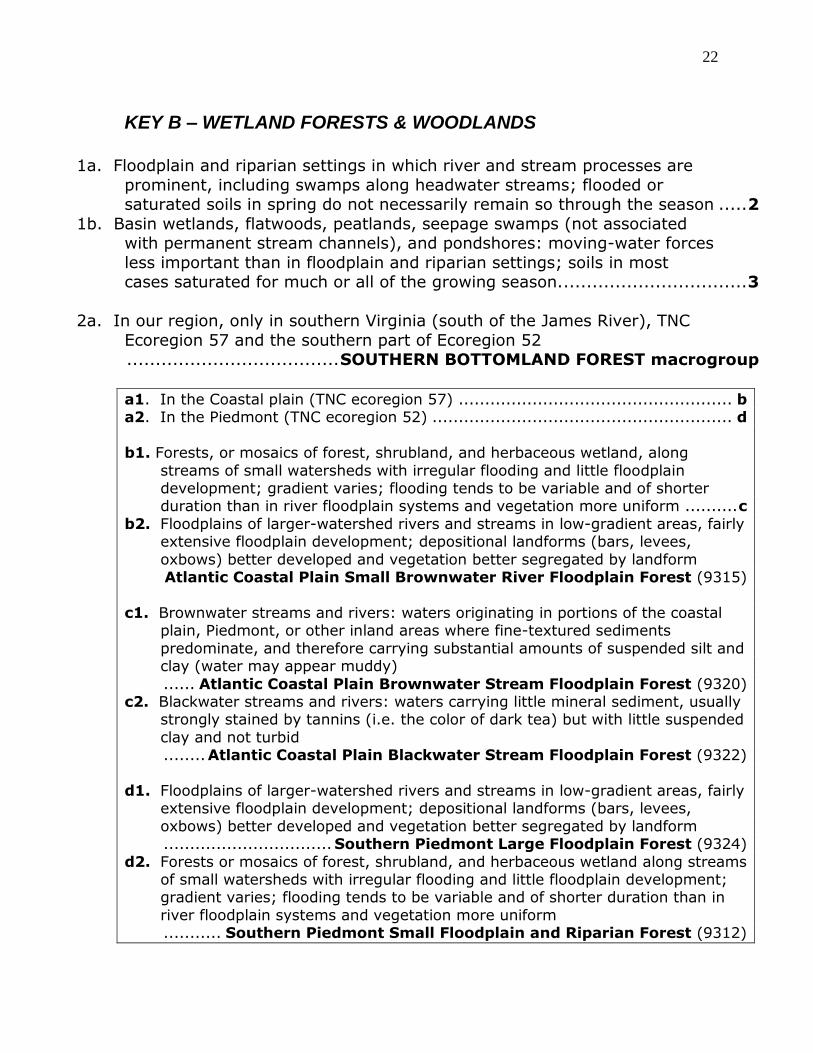
22
KEY B – WETLAND FORESTS & WOODLANDS
1a. Floodplain and riparian settings in which river and stream processes are
prominent, including swamps along headwater streams; flooded or saturated soils in spring do not necessarily remain so through the season ..... 2
1b. Basin wetlands, flatwoods, peatlands, seepage swamps (not associated with permanent stream channels), and pondshores: moving-water forces
less important than in floodplain and riparian settings; soils in most cases saturated for much or all of the growing season................................. 3
2a. In our region, only in southern Virginia (south of the James River), TNC
Ecoregion 57 and the southern part of Ecoregion 52 ..................................... SOUTHERN BOTTOMLAND FOREST macrogroup
a1. In the Coastal plain (TNC ecoregion 57) .................................................... b a2. In the Piedmont (TNC ecoregion 52) ......................................................... d
b1. Forests, or mosaics of forest, shrubland, and herbaceous wetland, along
streams of small watersheds with irregular flooding and little floodplain development; gradient varies; flooding tends to be variable and of shorter duration than in river floodplain systems and vegetation more uniform .......... c
b2. Floodplains of larger-watershed rivers and streams in low-gradient areas, fairly extensive floodplain development; depositional landforms (bars, levees,
oxbows) better developed and vegetation better segregated by landform Atlantic Coastal Plain Small Brownwater River Floodplain Forest (9315)
c1. Brownwater streams and rivers: waters originating in portions of the coastal
plain, Piedmont, or other inland areas where fine-textured sediments
predominate, and therefore carrying substantial amounts of suspended silt and clay (water may appear muddy)
...... Atlantic Coastal Plain Brownwater Stream Floodplain Forest (9320) c2. Blackwater streams and rivers: waters carrying little mineral sediment, usually
strongly stained by tannins (i.e. the color of dark tea) but with little suspended
clay and not turbid ........ Atlantic Coastal Plain Blackwater Stream Floodplain Forest (9322)
d1. Floodplains of larger-watershed rivers and streams in low-gradient areas, fairly
extensive floodplain development; depositional landforms (bars, levees,
oxbows) better developed and vegetation better segregated by landform ................................ Southern Piedmont Large Floodplain Forest (9324)
d2. Forests or mosaics of forest, shrubland, and herbaceous wetland along streams of small watersheds with irregular flooding and little floodplain development; gradient varies; flooding tends to be variable and of shorter duration than in
river floodplain systems and vegetation more uniform ........... Southern Piedmont Small Floodplain and Riparian Forest (9312)

23
2b. More widespread; all areas north of the James River, Virginia .............................. NORTHEASTERN FLOODPLAIN FOREST macrogroup
a1. Floodplains and stream forests in the southwestern part of the region, along
rivers of the Ohio River drainage (more or less TNC ecoregions 49, 50, 51) ... b a2. Floodplains and stream forests elsewhere in the region, draining to the
Atlantic ................................................................................................... c
b1. Floodplains of larger-watershed rivers and streams in low-gradient areas, fairly extensive floodplain development; depositional landforms (bars, levees, oxbows) better developed and vegetation better segregated by landform
...................................... South-Central Interior Large Floodplain (9334) b2. Forests or mosaics of forest, shrubland, and herbaceous wetland along streams
of small watersheds with irregular flooding and little floodplain development; gradient varies; flooding tends to be variable and of shorter duration than in river floodplain systems and vegetation more uniform
................. South-Central Interior Small Stream and Riparian (9335)***
c1. Floodplains of rivers and streams on the Atlantic coastal plain, north to New Jersey .............. Northern Atlantic Coastal Plain Stream and River (4157)
c2. Floodplains and stream forests interior to the coastal plain, or north of New Jersey ................................................................................................... d
d1. Floodplain forests of northern New England and northern New York (USFS Sections M211 and 211A-211E)
...................................... Laurentian-Acadian Floodplain Systems (9144) d2. Floodplain and riparian forests in the remainder of the region (southern New
England and New York to central Virginia and eastern West Virginia)............. e
e1. Floodplains of larger-watershed rivers and streams in low-gradient areas, fairly
extensive floodplain development; depositional landforms (bars, levees, oxbows) better developed and vegetation better segregated by landform
.......................................... Central Appalachian River Floodplain (9333)
e2. Forests or mosaics of forest, shrubland, and herbaceous wetland along streams of small watersheds with irregular flooding and little floodplain development;
gradient varies; flooding tends to be variable and of shorter duration than in river floodplain systems and vegetation more uniform; system includes headwater seepage swamps that drain to the stream
........................... Central Appalachian Small Stream Riparian (9331)***
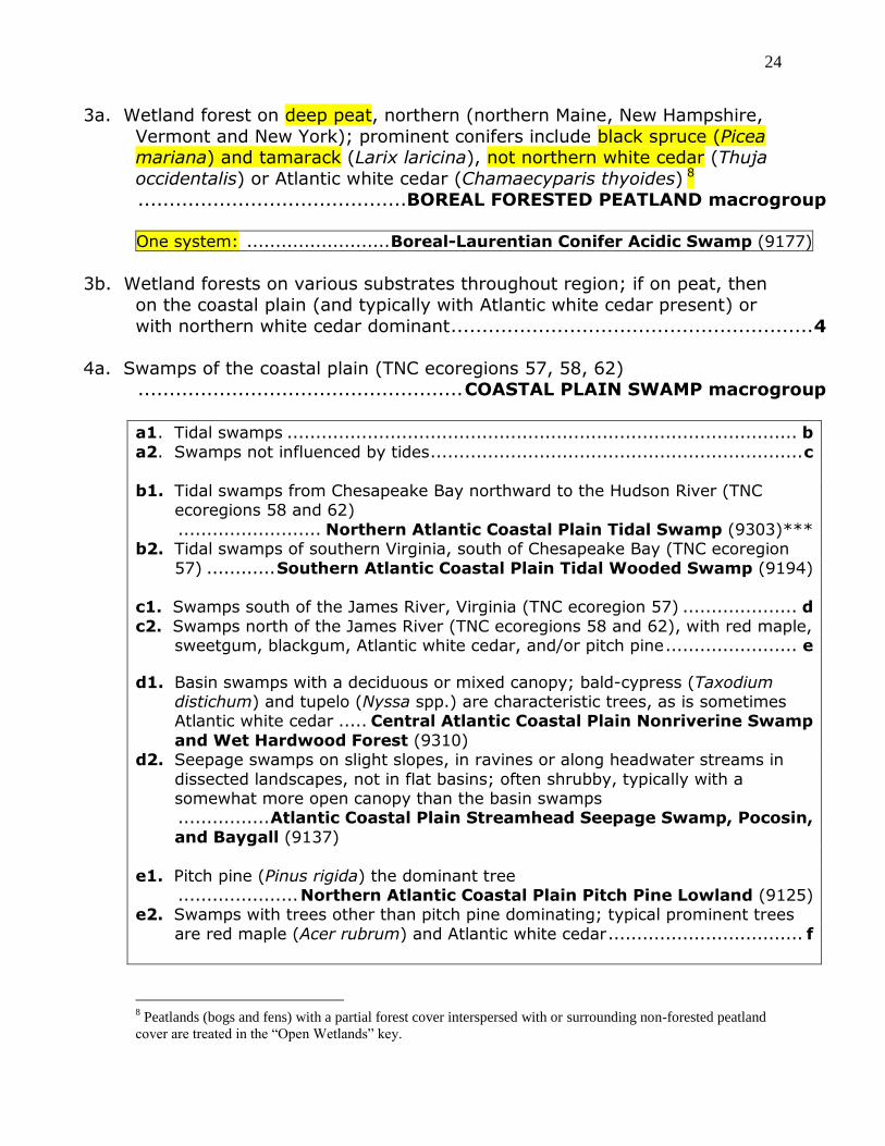
24
3a. Wetland forest on deep peat, northern (northern Maine, New Hampshire,
Vermont and New York); prominent conifers include black spruce (Picea mariana) and tamarack (Larix laricina), not northern white cedar (Thuja
occidentalis) or Atlantic white cedar (Chamaecyparis thyoides) 8 ........................................... BOREAL FORESTED PEATLAND macrogroup
One system: ......................... Boreal-Laurentian Conifer Acidic Swamp (9177)
3b. Wetland forests on various substrates throughout region; if on peat, then
on the coastal plain (and typically with Atlantic white cedar present) or
with northern white cedar dominant .......................................................... 4
4a. Swamps of the coastal plain (TNC ecoregions 57, 58, 62) .................................................... COASTAL PLAIN SWAMP macrogroup
a1. Tidal swamps ......................................................................................... b
a2. Swamps not influenced by tides ................................................................. c
b1. Tidal swamps from Chesapeake Bay northward to the Hudson River (TNC
ecoregions 58 and 62)
......................... Northern Atlantic Coastal Plain Tidal Swamp (9303)*** b2. Tidal swamps of southern Virginia, south of Chesapeake Bay (TNC ecoregion
57) ............ Southern Atlantic Coastal Plain Tidal Wooded Swamp (9194) c1. Swamps south of the James River, Virginia (TNC ecoregion 57) .................... d
c2. Swamps north of the James River (TNC ecoregions 58 and 62), with red maple, sweetgum, blackgum, Atlantic white cedar, and/or pitch pine ....................... e
d1. Basin swamps with a deciduous or mixed canopy; bald-cypress (Taxodium distichum) and tupelo (Nyssa spp.) are characteristic trees, as is sometimes Atlantic white cedar ..... Central Atlantic Coastal Plain Nonriverine Swamp
and Wet Hardwood Forest (9310) d2. Seepage swamps on slight slopes, in ravines or along headwater streams in
dissected landscapes, not in flat basins; often shrubby, typically with a somewhat more open canopy than the basin swamps
................ Atlantic Coastal Plain Streamhead Seepage Swamp, Pocosin,
and Baygall (9137)
e1. Pitch pine (Pinus rigida) the dominant tree ..................... Northern Atlantic Coastal Plain Pitch Pine Lowland (9125) e2. Swamps with trees other than pitch pine dominating; typical prominent trees
are red maple (Acer rubrum) and Atlantic white cedar .................................. f
8 Peatlands (bogs and fens) with a partial forest cover interspersed with or surrounding non-forested peatland
cover are treated in the “Open Wetlands” key.

25
f1. Saturated, peat-based swamps, usually dominated by Atlantic white cedar,
sometimes mixed with red maple ...................... Northern Atlantic Coastal Plain Basin Peat Swamp (9343)
f2. Hardwood swamps of seasonally flooded but not permanently saturated basins; mineral or muck soils, typical trees include red maple, sweetgum (Liquidambar
styraciflua), blackgum (Nyssa sylvatica), and green ash (Acer pennsylvanicum) ........ Northern Atlantic Coastal Plain Basin Swamp and Wet Hardwood Forest (9342)
4b. Swamps interior from the coastal plain........................................................ 5
5a. Swamps characterized by wetland oaks (generally > 15% relative canopy cover), occurring mostly in the southern portions of the region, with
disjunct occurrences in the clayplain forests of Vermont’s Champlain Valley .................................. CENTRAL HARDWOOD SWAMP macrogroup
a1. Sinkholes and sinkhole ponds formed by karst collapse in limestone or dolomite areas, typically in isolated upland depressions; rare in the northeast
..................... Central Interior Highlands and Appalachian Sinkhole and Depression Pond (9160)***
a2. Other wetlands, not karst collapse features ................................................ b b1. Isolated wetlands of small, shallow basins, typically set within upland forests
rather than being part of an extensive wetland system ........................... c b2. More extensive (at least historically) wetlands of lakeplains in the Champlain
Valley (Vermont), on soils that may dry out over the course of the season ................................... North-Central Interior Wet Flatwoods (9186)***
c1. Isolated wetlands north or west of the Virginia-Maryland Piedmont (TNC 52), with a perched water table, including shallow depressions in glacial plains;
swamp white oak (Quercus bicolor) and/or pin oak (Q. palustris) characteristic and often dominant ............. North-Central Interior Wet Flatwoods (9186)
c2. Piedmont ecoregion (TNC 52) of Virginia and Maryland; overcup oak (Q. lyrata)
and willow oak (Q. phellos) characteristic (pin oak and swamp white oak may also be present) ............ Piedmont Upland Depression Swamp (9302)***
5b. Swamps characterized by other trees: spruce, fir, hemlock, northern white cedar, red maple, blackgum, etc.; throughout the region, widespread in
the northern (glaciated) portions and mostly at higher elevations in the southern portions .................................. NORTHERN SWAMP macrogroup
a1. Wetlands in the higher Allegheny Mountains at elevations of > 1200 m (4000’),
physiognomy and size varies from small-patch isolated wetlands to large
complexes that may include areas of open peatland, wooded swamps, open mineral-soil wetlands, etc. ......................... High Allegheny Wetland (9356)
a2. Wetlands at lower elevations .................................................................... b
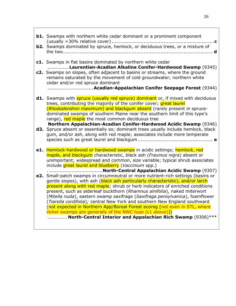
26
b1. Swamps with northern white cedar dominant or a prominent component (usually >30% relative cover) ................................................................... c
b2. Swamps dominated by spruce, hemlock, or deciduous trees, or a mixture of the two.................................................................................................. d
c1. Swamps in flat basins dominated by northern white cedar .............. Laurentian-Acadian Alkaline Conifer-Hardwood Swamp (9345)
c2. Swamps on slopes, often adjacent to basins or streams, where the ground remains saturated by the movement of cold groundwater; northern white
cedar and/or red spruce dominant .............................. Acadian-Appalachian Conifer Seepage Forest (9344)
d1. Swamps with spruce (usually red spruce) dominant or, if mixed with deciduous trees, contributing the majority of the conifer cover; great laurel
(Rhododendron maximum) and blackgum absent (rarely present in spruce-dominated swamps of southern Maine near the southern limit of this type’s range), red maple the most common deciduous tree
Northern Appalachian-Acadian Conifer-Hardwood Acidic Swamp (9346) d2. Spruce absent or essentially so; dominant trees usually include hemlock, black
gum, and/or ash, along with red maple; associates include more temperate species such as great laurel and blackgum ................................................. e
e1. Hemlock-hardwood or hardwood swamps in acidic settings; hemlock, red maple, and blackgum characteristic, black ash (Fraxinus nigra) absent or
unimportant; widespread and common, size variable; typical shrub associates include great laurel and blueberry (Vaccinium spp.)
. ................................... North-Central Appalachian Acidic Swamp (9307)
e2. Small-patch swamps in circumneutral or more nutrient-rich settings (basins or gentle slopes), with ash (black ash particularly characteristic), and/or larch
present along with red maple; shrub or herb indicators of enriched conditions present, such as alderleaf buckthorn (Rhamnus alnifolia), naked miterwort (Mitella nuda), eastern swamp saxifrage (Saxifraga pensylvanica), foamflower
(Tiarella cordifolia); central New York and southern New England southward (not expected in Northern App/Boreal Forest ecoreg [not even in STL, where
richer swamps are generally of the NWC type (c1 above)]) ............. North-Central Interior and Appalachian Rich Swamp (9306)***

27

28
KEY C – HERB/SHRUB AND SPARSELY VEGETATED UPLANDS
1a. Areas near or above treeline, mostly above 915 m (3000’); restricted to
the northern Appalachian Mountains in Maine and New Hampshire, with small occurrences in Vermont and New York ................ ALPINE macrogroup
a1. True alpine dwarf-shrub and herbaceous vegetation of the region’s highest
elevations above treeline, with one or more of these diagnostic species:
pincushion plant (Diapensia lapponica), Lapland rosebay (Rhododendron lapponicum), mossplant (Harrimanella hypnoides), alpine azalea (Loiseleuria procumbens), blue mountainheath (Phyllodoce caerulea), and Bigelow’s sedge
(Carex begelowii); alpine bilberry (Vaccinium uliginosum) typical and often dominant ............................... Acadian-Appalachian Alpine Tundra (5210)
a2. Dwarf-shrub, herbaceous, and stunted woodland vegetation near or above treeline, lacking the true alpine species; dominants include black spruce, mountain paper birch (Betula papyrifera var. cordifolia), alpine bilberry,
crowberry (Empetrum spp.), sheep laurel (Kalmia angustifolia), bog Labrador tea (Ledum groenlandicum); small Sphagnum wetlands with cranberry
(Vaccinium macrocarpon, V. oxycoccos) and cloudberry (Rubus chamaemorus) etc., may occur in bedrock depressions; extensive areas at treeline may be dominated by krummholz (dense mats of shrub-form spruce, fir, and birch)
............................................. Acadian-Appalachian Subalpine Woodland and Heath-Krummholz (5320)
1b. Areas not near treeline, though may be on tops of hills and mountains; various landscape positions...................................................................... 2
2a. Rock outcrops, summits, and cliffs, including bedrock shorelines, some
sparsely vegetated ................................................................................. 3 2b. Cobble or sandy shores [CF: only cobble shores are in 3a2], coastal
grasslands/shrublands, and reverting fields ............................................... 7
3a. Open rocky coast along the Atlantic shore, usually in a narrow band; often sparsely vegetated but sometimes with dwarf shrub or herbaceous
vegetation; mostly north of Cape Cod ............... ROCKY COAST macrogroup
a1. Consolidated rock substrate; rocky shores of various heights and slopes;
vegetation mostly confined to cracks in the bedrock ....................................... Acadian-North Atlantic Rocky Coast (3189)***
a2. Loose cobble rock substrate, forming a rock beach ................................................... North Atlantic Cobble Shore (3132)***
3b. Inland from the Atlantic shoreline ............................................................... 4
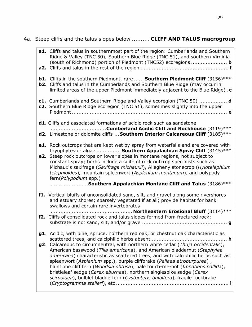
29
4a. Steep cliffs and the talus slopes below .......... CLIFF AND TALUS macrogroup
a1. Cliffs and talus in southernmost part of the region: Cumberlands and Southern
Ridge & Valley (TNC 50), Southern Blue Ridge (TNC 51), and southern Virginia (south of Richmond) portion of Piedmont (TNC52) ecoregions ...................... b
a2. Cliffs and talus in the rest of the region ...................................................... f
b1. Cliffs in the southern Piedmont, rare ..... Southern Piedmont Cliff (3156)***
b2. Cliffs and talus in the Cumberlands and Southern Blue Ridge (may occur in limited areas of the upper Piedmont immediately adjacent to the Blue Ridge) . c
c1. Cumberlands and Southern Ridge and Valley ecoregion (TNC 50) ................. d c2. Southern Blue Ridge ecoregion (TNC 51), sometimes slightly into the upper
Piedmont ............................................................................................... e d1. Cliffs and associated formations of acidic rock such as sandstone
.................................. Cumberland Acidic Cliff and Rockhouse (3119)*** d2. Limestone or dolomite cliffs ... Southern Interior Calcareous Cliff (3185)***
e1. Rock outcrops that are kept wet by spray from waterfalls and are covered with
bryophytes or algae ............... Southern Appalachian Spray Cliff (3145)***
e2. Steep rock outcrops on lower slopes in montane regions, not subject to constant spray; herbs include a suite of rock outcrop specialists such as
Michaux's saxifrage (Saxifraga michauxii), Allegheny stonecrop (Hylotelephium telephioides), mountain spleenwort (Asplenium montanum), and polypody fern(Polypodium spp.)
.......................Southern Appalachian Montane Cliff and Talus (3186)***
f1. Vertical bluffs of unconsolidated sand, silt, and gravel along some rivershores and estuary shores; sparsely vegetated if at all; provide habitat for bank swallows and certain rare invertebrates
.................................................. Northeastern Erosional Bluff (3114)*** f2. Cliffs of consolidated rock and talus slopes formed from fractured rock;
substrate is not sand, silt, and/or gravel .................................................... g g1. Acidic, with pine, spruce, northern red oak, or chestnut oak characteristic as
scattered trees, and calciphilic herbs absent ............................................... h g2. Calcareous to circumneutral, with northern white cedar (Thuja occidentalis),
American basswood (Tilia americana), and American bladdernut (Staphylea americana) characteristic as scattered trees, and with calciphilic herbs such as
spleenwort (Asplenium spp.), purple cliffbrake (Pellaea atropurpurea) , bluntlobe cliff fern (Woodsia obtusa), pale touch-me-not (Impatiens pallida), bristleleaf sedge (Carex eburnea), northern singlespike sedge (Carex
scirpoidea), bulblet bladderfern (Cystopteris bulbifera), fragile rockbrake (Cryptogramma stelleri), etc ..................................................................... i

30
h1. Northern portions of region: Northern Appalachian – Boreal Forest ecoregion
(TNC 63), St. Lawrence / Champlain Valley ecoregion (TNC 64), and Great Lakes ecoregion (TNC 48), peripheral in Lower New England / Northern
Piedmont ecoregion (TNC 61) where spruce is present ...............................Laurentian-Acadian Acidic Cliff and Talus (3188)***
h2. Central and southern (but not southernmost) portions of region: Central Appalachian Forest (TNC 59), Western Allegheny Plateau (TNC 49), High Allegheny Plateau (TNC 60), and Lower New England / Northern Piedmont
(TNC 61) ecoregions ....................North-Central Appalachian Acidic Cliff and Talus (3154)***
i1. Northern parts of region: Northern Appalachian – Boreal Forest, St. Lawrence /
Champlain Valley, and Great Lakes ecoregions (TNC 63, 64, 48), except along
Lake Erie (USFS subsections 222Ia and 222Ib), peripheral in Lower New England / Northern Piedmont ecoregion (TNC 61) where northern white cedar
is present ....................... Laurentian-Acadian Calcareous Cliff and Talus (3144)*** i2. Southern portions of region: Central Appalachian Forest, Western Allegheny
Plateau, High Allegheny Plateau, and Lower New England / Northern Piedmont ecoregions (TNC 59, 60, 61), and subsections 222Ia and 222Ib of the Great
Lakes ecoregion (TNC 48) ......................................................................... j j1. West of the Appalachians: Western Allegheny Plateau and Great Lakes
ecoregions (TNC 49, 48) ............................. Central Interior Calcareous Cliff and Talus (3148)***
j2. Appalachian and eastward: Central Appalachian Forest, High Allegheny Plateau, and Lower New England / Northern Piedmont ecoregions (TNC 59, 60, 61)
....... North-Central Appalachian Circumneutral Cliff and Talus (3153)***
4b. Open rocky ridges, summits, and sideslopes ................................................ 5
5a. Sparsely vegetated rock outcrops (granitic domes and flatrock) in the
Southern Blue Ridge and southern Piedmont ecoregions (TNC 51 and 52) ......................................................................... FLATROCK macrogroup
a1. Smooth, curved outcrops of granite and related rocks, usually occurring as
knobs rather than summit ridges; crevices largely lacking; vegetation very
sparse except for mats forming in shallow depressions and around the edges; Southern Blue Ridge ecoregion (TNC 51), sometimes in the adjacent upper Piedmont on monadnocks . Southern Appalachian Granitic Dome (3126)***
a2. Flatrock formations at lower elevations in the eastern and central southern Piedmont (TNC ecoregion 52) on granite, mostly horizontal to gently sloping
.................. Southern Piedmont Granite Flatrock and Outcrop (3175)***
5b. Vegetation cover more continuous, or if somewhat sparse in rocky areas,
then north of the southern Appalachians ................................................... 6

31
6a. Rocky glades in the Central Appalachians, southern Piedmont, and Southern Blue Ridge ecoregions (TNC 59, 52, and 51); on slopes and
ridges; vegetation usually a mosaic of low shrubs and herbs with scattered trees, usually with a well-developed grassy layer, though open
rocky areas may also be extensive ..... GLADE AND SAVANNA macrogroup9
a1. Alvars: rare herbaceous or wooded-herbaceous communities on flat limestone
or dolostone pavement near the Great Lakes, flooded in the springtime and drying out over the season; limited in the Northeast to Jefferson County, New
York (USFS subsections 211Ee and 222Ie); common juniper (Juniperus communis), russet buffaloberry (Shepherdia canadensis), kinnikinnick (Arctostaphylos uva-ursi) characteristic shrubs; alvar grassland and pavement
vegetation with tufted hairgrass (Deschampsia caespitosa), dropseed (Sporobolus spp.), Crawe's sedge (Carex crawei), poverty oatgrass (Danthonia
spicata); sometimes interspersed with alvar woodlands featuring eastern red-cedar, northern white cedar, white ash, sugar maple, hop hornbeam (Ostrya virginiana), bur oak (Quercus macrocarpa), and others; typically in a mosaic of
grasslands, shrublands, woodlands, and open limestone pavement ........................................................................ Great Lakes Alvar (5458)
a2. Other glades and savannas, not alvars ...................................................... b b1. Grassy, prairie-like savannas (a.k.a. oak openings) with scattered oak trees
including black oak (Quercus velutina), white oak (Q. alba), and/or bur oak (Q. macrocarpa) on well-drained, coarse-textured glacially-derived soils; restricted
in the Northeast to a few locations in western New York’s Erie-Ontario lakeplain (USFS Section 222I, possibly at least historically extending into NW Pennsylvania); heath shrubs not prominent; known examples in this region are
primarily on dolomite knobs, historically and elsewhere on sand plains .......................................................... North-Central Oak Barrens (5411)
b2. Not as above ........................................................................................... c c1. Southwestern Virginia: Cumberland and Southern Ridge & Valley ecoregion
(TNC 50), rarely extending a short way north into the Central Appalachians ecoregion (TNC 59) ................................................................................. d
c2. Elsewhere in region ................................................................................. e
d1. Woodlands, sometimes with open grassy glades, on limestone or other calcareous substrate ....... Southern Ridge and Valley Calcareous Glade and Woodland (5464)
d2. Herb- or herb-shrub vegetation, sometimes with scattered trees, on acidic sandstone substrate
............................. Cumberland Sandstone Glade and Barrens (5414)***
9 This macrogroup was also covered in the Forest and Woodland key, as the degree of tree cover can be quite
variable. Two of the habitat systems in this macrogroup, Great Lakes Alvar and North-Central Oak Barrens
(both New York state only), are covered only under the Forest and Woodland key. This couplet refers to
habitat systems in the central and southern Appalachians and adjacent Piedmont.

32
e1. Southern portion of the Piedmont ecoregion (TNC 52) , extending into our region only south of the James River in Virginia; rare; canopy dominated most
commonly by eastern red-cedar and various oaks and pines, but also including white ash, winged elm (Ulmus alata), and eastern redbud (Cercis canadensis)
on higher-pH examples .. Southern Piedmont Glade and Barrens (5412)*** e2. Not in the southern Piedmont south of the James River ................................ f
f1. Woodlands and glades on calcareous substrate with chinkapin oak (Quercus muehlenbergii) characteristic, and pines and post oak (Q. stellata) generally
sparse or absent; Central Appalachians ecoregion (TNC 59), extending into the northern Piedmont (TNC 61) to southeastern New York; characteristic forbs include whorled milkweed (Asclepias verticillata), wild bergamot (Monarda
fistulosa), lyreleaf sage (Salvia lyrata), aromatic aster (Symphyotrichum oblongifolium), and false boneset (Brickellia eupatorioides); bristleleaf sedge
(Carex eburnea) a diagnostic herb (though not always present) ................. Central Appalachian Alkaline Glade and Woodland (5416)*** f2. Partly wooded glades and barrens developing on mafic rocks such as
greenstone or amphibolite, less commonly on felsic rock but not on calcareous rock; vegetation a patchy mosaic of open woodland and grassy herbaceous
openings; Southern Blue Ridge (TNC 51), upper Piedmont (portion of TNC 52), and southern Central Appalachian Forest (TNC 59) ecoregions, known in our region only from a few locations in Virginia and Maryland
.. Southern and Central Appalachian Mafic Glade and Barrens (5415)***
6b. Open rocky habitats, trees either absent, or if present, scattered and
stunted; mostly from northern Pennsylvania and New Jersey northward, or (rare in this region, only in Virginia’s Mount Rogers area) at the
highest elevations of the Southern Appalachians ................................................ OUTCROP/SUMMIT SCRUB macrogroup
a1. High-elevation grassy balds of the Southern Blue Ridge ecoregion (TNC 51),
present on our region only in Virginia in the Mount Rogers – Whitetop
Mountain area .......................... Southern Appalachian Grass and Shrub Bald (7127)***
a2. Outcrops and summits from northern New Jersey and Pennsylvania northward. ............................................................................................................ b
b1. Flat rock barrens of the Great Lakes region, known in our region only from one area of upstate New York, distinguished by the presence of jack pine on
sandstone pavement ............... Laurentian Acidic Rocky Outcrop (5463)*** b2. Rocky outcrops in other settings, mostly associated with hills or low summits ............................................................................................................. c

33
c1. Summits and outcrops of acidic rock, heath shrubs including lowbush blueberry
(Vaccinium angustifolium), sheep laurel (Kalmia angustifolia) , and/or huckleberry (Gaylussacia baccata) often present; scattered and stunted trees
of northern red oak, red spruce, and red or white pine may be present; usually small but sometimes extensive along low- to mid-elevation ridgelines
............. Northern Appalachian-Acadian Rocky Heath Outcrop (5462)*** c2. Summits and outcrops of circumneutral to calcareous rock (limestone,
dolomite, some basalts), with calciphilic plants such as bristleleaf sedge (Carex
eburnea) broadleaf sedge (Carex platyphylla), wreath goldenrod (Solidago caesia), spleenworts (Asplenium spp.), northern white cedar (Thuja
occidentalis), prairie goldenrod (Solidago ptarmicoides), bulblet bladderfern (Cystopteris bulbifera), and/or shrubby cinquefoil (Dasiphora fruticosa ssp. floribunda); typically small openings
...................... Laurentian-Acadian Calcareous Rocky Outcrop (5461)***
7a. Non-wooded upland areas along lakeshores (other than the Great Lakes)
and rivershores10, generally quite small . LAKE & RIVER SHORE macrogroup One system: ........................... Laurentian-Acadian Lakeshore Beach (3182)***
7b. Grasslands and shrublands not along lakeshores or rivershores ...................... 8
8a. Beaches, grasslands and shrublands along the immediate coasts of the
Atlantic Ocean or Great Lakes, maintained by exposure and fire; native plants predominate ..... COASTAL GRASSLAND & SHRUBLAND macrogroup
a1. Great Lakes shores ................................................................................. b
a2. Atlantic shores ........................................................................................ c
b1. Large stabilized dunes, mostly not immediately influenced by current shore
processes, sometimes developing on old glacial moraines and may be many meters above current water levels, not forming a mosaic with interspersed dune swales; vegetation varies from graminoid-dominated to shrubby to
scattered trees .............................................. Great Lakes Dune (3137)*** b2. Low dune ridges forming a mosaic of dune ridges and wet swales; most often
found where post-glacial streams entered an embayment and provided a dependable sand source; foredunes commonly 1-2 m high, with grasses (Ammophila breviligulata and Calamovilfa longifolia) and willows (Salix spp.)
most common; shrubs and trees developing on backdunes; dune swales typically featuring rushes (Juncus balticus, J. pelocarpus, J. nodosus), and
chairmaker's bulrush (Schoenoplectus americanus); possible in the Northeast only in western New York, and development of true ridge-and-swale morphology (as it is described from Michigan, for example) not confirmed
.................................................. Great Lakes Dune and Swale (9135)***
10
This statement refers to areas that are not regularly flooded. Most rivershore open habitats, even if not
apparently wetland, are subject to floodwaters at some frequency and are covered under the Open Wetlands
key, which includes floodplain habitats.

34
c1. Rare coastal heathlands and grasslands located back from active dune areas; trees sparse or absent (where trees are present, pitch pine and/or post oak
typical); dominated by heath shrubs, particularly blueberry, huckleberry, and bearberry (Arctostaphylos uva-ursi); goldenheather (Hudsonia spp.) also
characteristic along with native grasses/sedges such as little bluestem (Schizachyrium scoparium) and Pennsylvania sedge (Carex pensylvanica); scattered locales on Cape Cod and the nearby islands and on Long Island
........... Northern Atlantic Coastal Plain Heathland and Grassland (5275) c2. Sand beach and dune systems with actively moving sand along the immediate
shore .................................................................................................... d d1. Beaches occurring shoreward of dunes, vegetation sparse, annual forbs
prominent ........... Northern Atlantic Coastal Plain Sandy Beach (3124)*** d2. Dunes with more continuous vegetation, grasses prominent; may include
shrubby portions or occasional stunted pitch pine ............................ Northern Atlantic Coastal Plain Dune and Swale (7149)
8b. Grasslands and shrublands developing on lands that were cleared and are
now reverting to forest; widespread and common; non-native grasses are typical (though some have a native grass component); pasture
grasses and herbs common
............................... RUDERAL SHRUBLAND & GRASSLAND macrogroup
a1. Ruderal vegetation along powerline rights-of-way, generally maintained as low
vegetation by cutting; usually a patchwork of herb and shrub vegetation .............................................................. Powerline Right-of-Way (8302) a2. Habitats not along powerline rights-of-way ................................................ b
b1. Scrubby habitats dominated by non-native shrub species such as multiflora
rose (Rosa multiflora), honeysuckle (Lonicera spp.), and Asian bittersweet (Celastrus orbiculata); vegetation typically very dense
............................................................ Introduced Shrubland (8402)***
b2. Reverting old fields and pastures, mostly dominated by a mix of native and non-native species; cover varies from strongly herbaceous (where more
frequently mowed) to herb-shrub mix; maintained by mowing or burning, and those not maintained develop increasing shrub and tree cover
...................................................... Ruderal Upland - Old Field (8301)***

35

36
KEY D – HERBACEOUS AND HERB/SHRUB WETLANDS
1a. Tidal wetlands .......................................................................................... 2
1b. Non-tidal wetlands .................................................................................... 3
2a. Salt and brackish marshes, vegetated with graminoids, forbs, and (sometimes) shrubs11 ....................................... SALT MARSH macrogroup
a1. Marshes of the southeastern Virginia coast, south of the James River (TNC
ecoregion 57) ........................................... Atlantic Coastal Plain Embayed
Region Tidal Salt and Brackish Marsh (9261) a2. Marshes in more northerly parts of the Atlantic coast .................................. b
b1. Brackish intertidal marshes of estuaries; tall graminoids such as chairmaker's bulrush (Schoenoplectus americanus), common threesquare (Schoenoplectus
pungens), prairie cordgrass (Spartina pectinata) and cattails (Typha spp.) abundant; saltmeadow cordgrass (Spartina patens) and/or smooth cordgrass (Spartina alterniflora) may be present on lower reaches of the estuary; some
areas dominated by low forb vegetation including tidalmarsh amaranth (Amaranthus cannabinus), knotweed (Polygonum spp.), mudwort (Limosella
subulata), eastern grasswort (Lilaeopsis chinensis), hooded arrowhead (Sagittaria calycina) ................................................................................. c
b2. Salt marshes at estuary mouths and salt marshes or salt ponds behind sandy beaches ................................................................................................. d
c1. Brackish tidal marshes north of Cape Cod (Massachusetts) ........................................................... Acadian Estuary Marsh (9292)***
c2. Brackish tidal marshes from Cape Cod southward .................. Northern Atlantic Coastal Plain Brackish Tidal Marsh (9272)
d1. Saltmarshes east and north of Merrymeeting Bay, Maine, not associated with sand beach and dune systems ......... Acadian Coastal Salt Marsh (9278)***
d2. Saltmarshes south and west of Merrymeeting Bay, Maine .......................... Northern Atlantic Coastal Plain Tidal Salt Marsh (9282)
2b. Intertidal flats, either unvegetated, or with macroalgae the dominant plant
forms ........................................................... INTERTIDAL SHORE macrogroup
a1. Intertidal zones with a solid rock substrate; seaweeds often common .............................................. North Atlantic Rocky Intertidal (3190)***
a2. Sandy or muddy intertidal flats ................................................................. b
11
Freshwater tidal marshes are covered under the Emergent Marsh macrogroup

37
b1. Sand flats, often associated with beaches
...................................................... North Atlantic Tidal Sand Flat (3134) b2. Intertidal mud flats, common in coves and somewhat protected areas
................................................. North Atlantic Intertidal Mudflat (3133)
3a. Peat-based bogs and fens with heath shrubs such as leatherleaf (Chamaedaphne calyculata), bog laurel (Kalmia polifolia), sheep laurel,
etc. prominent; substrate of living and decomposing mosses, not mineral soil ....................................................................................................... 4
3b. Wetlands on mineral soil or muck; if mosses form a continuous ground layer, then mineral soil is present within 30 cm (6”) or so of the surface;
heath shrubs do not dominate the upper layer of vegetation ........................ 6
4a. Peatlands in the coastal plain (TNC ecoregions 62, 58, and 57), mostly in small isolated basins .................. COASTAL PLAIN PEATLAND macrogroup
a1. Peatlands of the central Atlantic coastal plain, extending into our region only in
southeastern Virginia (south of the James River, TNC ecoregion 57)
............... Atlantic Coastal Plain Peatland Pocosin and Canebrake (9121) a2. Peatlands in the coastal plain from northern New Jersey northward12
....................................... Atlantic Coastal Plain Northern Bog (9189)***
4b. Peatlands interior from the coastal plain ....................................................... 5
5a. Peatlands in glaciated territory13; in basins (not seepage slopes) varying in
size and hydrology from isolated kettleholes to extensive slow-draining shallow basins to lakeshore fens14 ....... NORTHERN PEATLAND macrogroup
a1. Alkaline fens, with calciphilic indicators including shrubby-cinquefoil (Dasiphora
fruticosa ssp. floribunda), bog birch (Betula pumila), yellow sedge (Carex
flava), dioecious sedge (Carex sterilis), fen grass of Parnassus (Parnassia glauca), golden ragwort (Packera aurea), Ontario lobelia (Lobelia kalmii), sageleaf willow (Salix candida) . Laurentian-Acadian Alkaline Fen (9198)***
a2. Acidic fens and bogs with a well-developed Sphagnum substrate; heath shrubs including leatherleaf (Chamaedaphne calyculata), bog Labrador tea (Ledum
groenlandicum), sheep laurel (Kalmia anglustifolia), rhodora (Rhododendron canadense), bog laurel (Kalmia polifolia), bog rosemary (Andromeda polifolia var. glaucophylla) usually form a dense layer or are prominent in patches;
calciphilic indicators are lacking ................................................................ b
12
Non-forested peatlands in the region between northern New Jersey and Chesapeake Bay are covered under
the Northern Atlantic Coastal Plain Pitch Pine Lowland, in the Wooded Wetlands key (Key B). 13
The glaciated part of the region includes New England, most of New York, and small parts of northwestern
and northeastern Pennsylvania 14
Midwestern prairie-like alkaline fens with a few rare occurrences in western Pennsylvania go to the second
half of this couplet.

38
b1. True bogs: raised bogs in Maine, northernmost Vermont, and limited portions
of the northern Adirondacks in which peat accumulation and vegetation is raised above the water table over at least the central (sometimes off-center)
part of the bog, so that all nutrients are derived from precipitation rather than groundwater (ombrotrophic); developing in large, more-or-less closed basins;
vegetation features a partial canopy or mosaic of open and wooded portions .. c
b2. Other peatlands15 throughout the region, with vegetation in contact with the water table, not distinctly raised above it (oligotrophic to minerotrophic); in
various sized basins, including glacial kettleholes ........................................ d
c1. Bogs along the eastern Maine coast (and a short ways inland, USFS subsection 211Cb) with a raised margin and flat center, graminoid carpets of tufted bulrush (Trichophorum caespitosum) characteristic, black crowberry
(Empetrum nigrum) and cloudberry (Rubus chamaemorus) are indicator species; rarely, in extreme maritime settings, developing as blanket bogs over
rock (in which case the noticeably raised margin is lacking) rather than as basin peatlands ............................................ Acadian Maritime Bog (9301)
c2. Bogs in more inland or southerly regions or, if near-coastal in subsection
211Cb, then lacking the maritime bog characteristics described above ................................................................. Boreal-Laurentian Bog (9354)
d1. Peatlands in the northern part of region: USFS Sections M211 or 211A,B,C,D,E ................................ Boreal-Laurentian-Acadian Acidic Basin Fen (9353)
d2. Peatlands in more southerly parts (though in the glaciated region): USFS Sections 221, 222, or 211F,G,I,J
........ North-Central Interior and Appalachian Acidic Peatland (9193)***
5b. Bogs and basin fens south of the glacial boundary, or seepage fens on
gentle slopes in the Division 202 portion of the glaciated region; almost
always very small .................................. CENTRAL APPALACHIAN PEATLAND macrogroup
a1. Small wetlands on gentle slopes, fed primarily by groundwater seepage ........ b
a2. Bogs and fens of various sizes in flat topographic basins, deep or shallow ....... c
b1. Southwestern Virginia: Southern Appalachians (TNC 51), occasionally in the Cumberlands (TNC 50) ecoregions
................................ Southern Appalachian Seepage Wetland (9259)*** b2. Central Appalachians, Northern Piedmont, and western Allegheny Plateau ................................ North-Central Appalachian Seepage Fen (9232)***
15
These are, in many cases, referred to as bogs (e.g. “kettlehole bog”) but because vegetation is in contact with
groundwater, they are technically fens.

39
c1. Midwestern shrubby fen system extending into the region only locally in the
Western Unglaciated Allegheny Plateau of Pennsylvania (Western Allegheny Plateau ecoregion, TNC 49); prairie grasses such as big bluestem (Andropogon
gerardii) or freshwater cordgrass (Spartina pectinata) often present ............ North-Central Interior Shrub-Graminoid Alkaline Fen (9184)***
c2. Bogs and fens in the Southern Blue Ridge, Central Appalachians, and Cumberland ecoregions (TNC 51, 59, 50) generally “small-patch” systems of a few hectares or less; Vegetation is a complex of zones or patches with
herbaceous-dominated areas as well as shrub thickets and often forested zones ............. Southern and Central Appalachian Bog and Fen (9309)***
6a. Artificially created wetlands, wetlands highly managed for water supply,
and wetlands strongly dominated by non-native plant species ............................................ MODIFIED/MANAGED MARSH macrogroup
a1. Wetlands strongly dominated by introduced species such as purple loosestrife
(Lythrum salicaria) or common reed (Phragmites australis), such that native plant species are minor or absent; cover may be herbaceous or mixed shrub-
herb ...... Introduced Wetland and Riparian Vegetation - Mixed (8411)*** a2. Artificially created wetlands, or wetlands highly managed for water supply
....................................................... Modified/Managed Marsh (8511)***
6b. Naturally occurring wetlands with a predominance of native plant species ....... 7
7a. Shallow ponds in isolated, usually small, sandy-rimmed groundwater
flooded basins of the Atlantic coastal plain, of varying depths but frequently shallow, in which the water level fluctuates (most commonly
dropping more or less steadily) over the growing season, resulting in a wetland with concentric rings of vegetation, including some areas of
herbaceous dominance and some rings of tree or shrub dominance ....................................................... COASTAL PLAIN POND macrogroup
a1. Coastal Plain of southernmost Virginia south (TNC ecoregion 57); small
wetlands in depressions within unconsolidated sediments, often resulting from
subsidence of limestone .......... Southern Atlantic Coastal Plain Depression Pondshore (9305)***
a2. Coastal Plain from the Delmarva peninsula north to southern Maine ..................................... Northern Atlantic Coastal Plain Pond (9283)***
7b. Marshes and wet meadows outside of the coastal plain, or if in the coastal
plain then not fitting the description above ................................................ 8

40
8a. Marshes of ponds or shores with standing water for most of the season
(including freshwater tidal areas); vegetation emergent, not strictly aquatic; most plants do not persist beyond the growing season; cattails,
pickerelweed, and tall rushes are typical, and shrubs may be present ............................................................. EMERGENT MARSH macrogroup
a1. Marshes associated with estuaries of the Great Lakes: limited areas of western
Pennsylvania and New York in our region
.................................. Great Lakes Freshwater Estuary and Delta (9268) a2. Marshes not along Great Lakes shores ....................................................... b
b1. Freshwater tidal marshes at the upper tidal reaches of estuaries ................... c b2. Other freshwater emergent marshes; widespread throughout region, best
developed in the glaciated portions ........................................ Laurentian-Acadian Freshwater Marsh (9405)
c1. Freshwater tidal marshes of southeastern Virginia (south of the James River, TNC ecoregion 57) ........................ Atlantic Coastal Plain Embayed Region
Tidal Freshwater Marsh (9276)*** c2. Freshwater tidal marshes of the Atlantic coast north of southeastern Virginia
(TNC ecoregions 58 and 62)
. Northern Atlantic Coastal Plain Fresh & Oligohaline Tidal Marsh (9293)
8b. Wet meadows and shrub marshes on substrates that are flooded for only
part of the season, if at all; vegetation is persistent and includes various combinations of sedges, grasses, and shrubs
.........................................WET MEADOW / SHRUB MARSH macrogroup
a1. Wetlands associated with sand dunes of the southeastern coastal plain; most
are permanently or semipermanently flooded with freshwater but are affected by salt spray or overwash during periodic storm events; in this region only in
southeastern Virginia (south of the James River, TNC ecoregion 57) ..................... Southeastern Coastal Plain Interdunal Wetland (9257)*** a2. Wetlands in other settings throughout the region; widespread and variable,
best developed in the glaciated portions ......................... Laurentian-Acadian Wet Meadow-Shrub Swamp (9406)
* * * * *

41
Literature Cited
Comer, P., D. Faber-Langendoen, R. Evans, S. Gawler, C. Josse, G. Kittel, S. Menard, M. Pyne, M.
Reid, K. Schulz, K. Snow, and J. Teague. 2003. Ecological systems of the United States: A working
classification of U.S. terrestrial systems. NatureServe, Arlington, VA.
FGDC (Federal Geographic Data Committee), Vegetation Subcommittee. 2008. National Vegetation
Classification Standard, Version 2. FGDC-STD-005-2008 (Version 2). available at:
http://www.fgdc.gov/standards/projects/FGDC-standards-projects/vegetation/
Gawler, S.C. 2008. Northeastern Terrestrial Wildlife Habitat Classification. Report to the Virginia
Department of Game and Inland Fisheries on behalf of the Northeast Association of Fish and Wildlife
Agencies and the National Fish and Wildlife Foundation. NatureServe, Boston, Massachusetts. 102 pp.
in Gawler et al 2008.
Gawler, S.C., M. G. Anderson, A. P. Olivero, and M. Clark. 2008. The Northeast Habitat Classification
and Mapping Project Final Report. a report to the Virginia Department of Game and Inland Fisheries on
behalf of the Northeast Association of Fish and Wildlife Agencies for the National Fish and Wildlife
Foundation (NFWF Project 2006-0181-003). NatureServe, Boston, Massachusetts.
Groves, C.R., D.B. Jensen, L.L. Valutis, K.H. Redford, M.L. Shaffer, J.M. Scott, J.V. Baumgartner, J.V.
Higgins, M.W. Beck, and M.G. Anderson. 2002. Planning for biodiversity conservation: putting
conservation science into practice. Bioscience 52: 499-512.
Kartesz, J. T. 1999. A synonymized checklist and atlas with biological attributes for the vascular flora of
the United States, Canada, and Greenland. First edition. In: J. T. Kartesz and C. A. Meacham. Synthesis
of the North American Flora, Version 1.0. North Carolina Botanical Garden, Chapel Hill, NC.
MRLC (Multi-Resolution Land Characteristics Consortium) 2008. NLCD 2001 Mapping Zones. at:
http://www.mrlc.gov/nlcd.php , accessed various dates to 22 Sep 2008.
NatureServe. 2008a. Field Key to Ecological Systems of Map Zones 54, 57, 59 60, and 61:
Southern Piedmont, Southern Appalachia, Northeastern Piedmont, Chesapeake Bay, and Northern
Appalachia (United States). Terrestrial Ecology Department, NatureServe, Arlington, VA. 24 pp.
NatureServe. 2008b. Field Key to the Ecological Systems of Map Zones 63, 64, 65, and 66:
Finger Lakes, Northeastern Highlands, Connecticut River Basin and Highlands, and
The North Woods (United States). Terrestrial Ecology Department, NatureServe, Arlington, VA. 33 pp.

42
Appendix A: Cross-reference to plant common names and scientific names. See p. 46 for a listing alphabetized by common name.
alphabetized by scientific name
Scientific Name Common name
Abies sp. fir
Abies balsamea balsam fir
Abies fraseri Fraser fir
Acer barbatum southern sugar maple
Acer leucoderme chalk maple
Acer platanoides Norway maple
Acer rubrum red maple
Acer saccharinum silver maple
Acer saccharum sugar maple
Actaea racemosa black bugbane
Adiantum pedatum northern maidenhair
Aesculus flava yellow buckeye
Ageratina altissima var. roanensis white snakeroot
Ailanthus altissima tree of heaven
Amaranthus cannabinus tidalmarsh amaranth
Ammophila breviligulata American beachgrass
Andromeda polifolia bog rosemary
Andropogon gerardii big bluestem
Arctostaphylos uva-ursi kinnikinnick
Arisaema triphyllum Jack in the pulpit
Asclepias verticillata whorled milkweed
Asplenium sp. spleenwort
Asplenium montanum mountain spleenwort
Betula alleghaniensis yellow birch
Betula lenta sweet birch
Betula papyrifera paper birch
Betula papyrifera var. cordifolia mountain paper birch
Betula pumila bog birch
Brickellia eupatorioides false boneset
Calamovilfa longifolia prairie sandreed
Carex bigelowii Bigelow's sedge
Carex crawei Crawe's sedge
Carex eburnea bristleleaf sedge
Carex flava yellow sedge
Carex pensylvanica Pennsylvania sedge
Carex platyphylla broadleaf sedge
Carex scirpoidea northern singlespike sedge
Carex sterilis dioecious sedge

43
Carya sp. hickory
Carya alba mockernut hickory
Carya ovalis red hickory
Carya ovata shagbark hickory
Caulophyllum thalictroides blue cohosh
Celastrus orbiculata Asian bittersweet
Cercis canadensis eastern redbud
Chamaecyparis thyoides Atlantic white-cedar
Chamaedaphne calyculata leatherleaf
Cryptogramma stelleri fragile rockbrake
Cystopteris bulbifera bulblet bladderfern
Danthonia spicata poverty oatgrass
Dasiphora fruticosa shrubby-cinquefoil
Deschampsia caespitosa tufted hairgrass
Diapensia lapponica pincushion plant
Dryopteris campyloptera mountain woodfern
Eleocharis acicularis needle spikerush
Empetrum sp. crowberry
Euonymus obovatus running strawberry bush
Fagus grandifolia American beech
Fraxinus sp. ash
Fraxinus americana white ash
Fraxinus nigra black ash
Fraxinus pennsylvanica green ash
Galium aparine stickywilly
Gaylussacia sp. huckleberry
Gaylussacia ursina bear huckleberry
Halesia tetraptera mountain silverbell
Harrimanella hypnoides mossplant
Hexastylis sp. heartleaf
Hexastylis arifolia var. ruthii Ruth's littlebrownjug
Hudsonia sp. goldenheather
Hydrangea arborescens wild hydrangea
Hylotelephium telephioides Allegheny stonecrop
Impatiens pallida pale touch-me-not
Juglans nigra black walnut
Juncus balticus Baltic rush
Juncus nodosus knotted rush
Juniperus communis common juniper
Juniperus virginiana eastern red-cedar
Kalmia angustifolia sheep laurel
Kalmia latifolia mountain laurel
Kalmia polifolia bog laurel
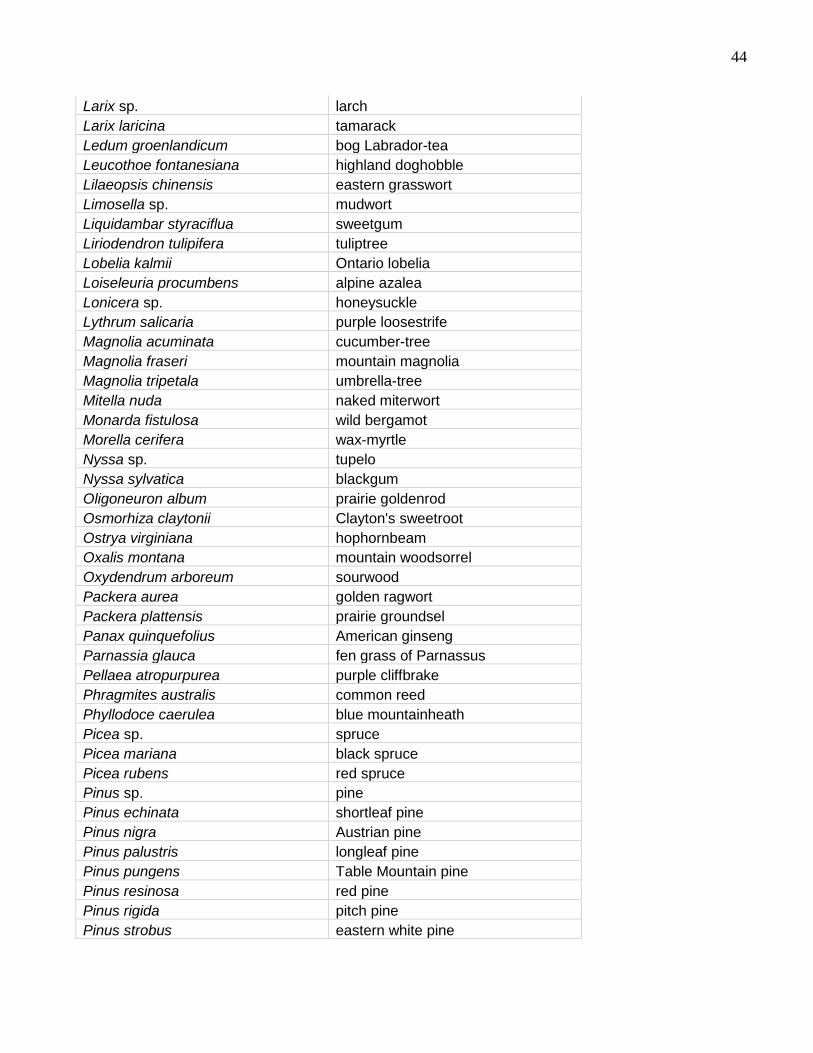
44
Larix sp. larch
Larix laricina tamarack
Ledum groenlandicum bog Labrador-tea
Leucothoe fontanesiana highland doghobble
Lilaeopsis chinensis eastern grasswort
Limosella sp. mudwort
Liquidambar styraciflua sweetgum
Liriodendron tulipifera tuliptree
Lobelia kalmii Ontario lobelia
Loiseleuria procumbens alpine azalea
Lonicera sp. honeysuckle
Lythrum salicaria purple loosestrife
Magnolia acuminata cucumber-tree
Magnolia fraseri mountain magnolia
Magnolia tripetala umbrella-tree
Mitella nuda naked miterwort
Monarda fistulosa wild bergamot
Morella cerifera wax-myrtle
Nyssa sp. tupelo
Nyssa sylvatica blackgum
Oligoneuron album prairie goldenrod
Osmorhiza claytonii Clayton's sweetroot
Ostrya virginiana hophornbeam
Oxalis montana mountain woodsorrel
Oxydendrum arboreum sourwood
Packera aurea golden ragwort
Packera plattensis prairie groundsel
Panax quinquefolius American ginseng
Parnassia glauca fen grass of Parnassus
Pellaea atropurpurea purple cliffbrake
Phragmites australis common reed
Phyllodoce caerulea blue mountainheath
Picea sp. spruce
Picea mariana black spruce
Picea rubens red spruce
Pinus sp. pine
Pinus echinata shortleaf pine
Pinus nigra Austrian pine
Pinus palustris longleaf pine
Pinus pungens Table Mountain pine
Pinus resinosa red pine
Pinus rigida pitch pine
Pinus strobus eastern white pine
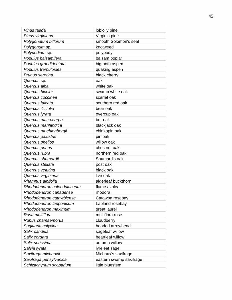
45
Pinus taeda loblolly pine
Pinus virginiana Virginia pine
Polygonatum biflorum smooth Solomon's seal
Polygonum sp. knotweed
Polypodium sp. polypody
Populus balsamifera balsam poplar
Populus grandidentata bigtooth aspen
Populus tremuloides quaking aspen
Prunus serotina black cherry
Quercus sp. oak
Quercus alba white oak
Quercus bicolor swamp white oak
Quercus coccinea scarlet oak
Quercus falcata southern red oak
Quercus ilicifolia bear oak
Quercus lyrata overcup oak
Quercus macrocarpa bur oak
Quercus marilandica blackjack oak
Quercus muehlenbergii chinkapin oak
Quercus palustris pin oak
Quercus phellos willow oak
Quercus prinus chestnut oak
Quercus rubra northern red oak
Quercus shumardii Shumard's oak
Quercus stellata post oak
Quercus velutina black oak
Quercus virginiana live oak
Rhamnus alnifolia alderleaf buckthorn
Rhododendron calendulaceum flame azalea
Rhododendron canadense rhodora
Rhododendron catawbiense Catawba rosebay
Rhododendron lapponicum Lapland rosebay
Rhododendron maximum great laurel
Rosa multiflora multiflora rose
Rubus chamaemorus cloudberry
Sagittaria calycina hooded arrowhead
Salix candida sageleaf willow
Salix cordata heartleaf willow
Salix serissima autumn willow
Salvia lyrata lyreleaf sage
Saxifraga michauxii Michaux's saxifrage
Saxifraga pensylvanica eastern swamp saxifrage
Schizachyrium scoparium little bluestem

46
Schoenoplectus americanus chairmaker's bulrush
Schoenoplectus pungens common threesquare
Shepherdia canadensis russet buffaloberry
Solidago caesia wreath goldenrod
Sorbus americana American mountain-ash
Sorbus decora northern mountain-ash
Spartina alterniflora smooth cordgrass
Spartina patens saltmeadow cordgrass
Spartina pectinata prairie cordgrass
Sporobolus sp. dropseed
Staphylea trifolia American bladdernut
Symphyotrichum depauperatum serpentine aster
Symphyotrichum oblongifolium aromatic aster
Taxodium distichum bald-cypress
Thalictrum macrostylum piedmont meadowrue
Thuja occidentalis northern white cedar
Tiarella sp. foamflower
Tilia americana American basswood
Trichophorum caespitosum tufted bulrush
Trillium grandiflorum white trillium
Tsuga sp. hemlock
Tsuga canadensis eastern hemlock
Typha sp. cattail
Ulmus alata winged elm
Vaccinium sp. blueberry
Vaccinium macrocarpon cranberry
Vaccinium uliginosum bog blueberry or bilberry
Woodsia obtusa bluntlobe cliff fern

47
alphabetized by common name
Common name Scientific Name
alderleaf buckthorn Rhamnus alnifolia
Allegheny stonecrop Hylotelephium telephioides
alpine azalea Loiseleuria procumbens
American basswood Tilia americana
American beachgrass Ammophila breviligulata
American beech Fagus grandifolia
American bladdernut Staphylea trifolia
American ginseng Panax quinquefolius
American mountain-ash Sorbus americana
aromatic aster Symphyotrichum oblongifolium
ash Fraxinus sp.
Asian bittersweet Celastrus orbiculata
Atlantic white-cedar Chamaecyparis thyoides
Austrian pine Pinus nigra
autumn willow Salix serissima
bald-cypress Taxodium distichum
balsam fir Abies balsamea
balsam poplar Populus balsamifera
Baltic rush Juncus balticus
bear huckleberry Gaylussacia ursina
bear oak Quercus ilicifolia
big bluestem Andropogon gerardii
Bigelow's sedge Carex bigelowii
bigtooth aspen Populus grandidentata
black ash Fraxinus nigra
black bugbane Actaea racemosa
black cherry Prunus serotina
black oak Quercus velutina
black spruce Picea mariana
black walnut Juglans nigra
blackgum Nyssa sylvatica
blackjack oak Quercus marilandica
blue cohosh Caulophyllum thalictroides
blue mountainheath Phyllodoce caerulea
blueberry Vaccinium sp.
bluntlobe cliff fern Woodsia obtusa
bog birch Betula pumila
bog blueberry Vaccinium uliginosum
bog Labrador-tea Ledum groenlandicum
bog laurel Kalmia polifolia

48
bog rosemary Andromeda polifolia
bristleleaf sedge Carex eburnea
broadleaf sedge Carex platyphylla
bulblet bladderfern Cystopteris bulbifera
bur oak Quercus macrocarpa
Catawba rosebay Rhododendron catawbiense
cattail Typha sp.
chairmaker's bulrush Schoenoplectus americanus
chalk maple Acer leucoderme
chestnut oak Quercus prinus
chinkapin oak Quercus muehlenbergii
Clayton's sweetroot Osmorhiza claytonii
cloudberry Rubus chamaemorus
common juniper Juniperus communis
common reed Phragmites australis
common threesquare Schoenoplectus pungens
cranberry Vaccinium macrocarpon
Crawe's sedge Carex crawei
crowberry Empetrum sp.
cucumber-tree Magnolia acuminata
dioecious sedge Carex sterilis
dropseed Sporobolus sp.
eastern grasswort Lilaeopsis chinensis
eastern hemlock Tsuga canadensis
eastern redbud Cercis canadensis
eastern red-cedar Juniperus virginiana
eastern swamp saxifrage Saxifraga pensylvanica
eastern white pine Pinus strobus
false boneset Brickellia eupatorioides
fen grass of Parnassus Parnassia glauca
fir Abies sp.
flame azalea Rhododendron calendulaceum
foamflower Tiarella sp.
fragile rockbrake Cryptogramma stelleri
Fraser fir Abies fraseri
golden ragwort Packera aurea
goldenheather Hudsonia sp.
great laurel Rhododendron maximum
green ash Fraxinus pennsylvanica
heartleaf Hexastylis sp.
heartleaf willow Salix cordata
hemlock Tsuga sp.
hickory Carya sp.

49
highland doghobble Leucothoe fontanesiana
honeysuckle Lonicera sp.
hooded arrowhead Sagittaria calycina
hophornbeam Ostrya virginiana
huckleberry Gaylussacia sp.
Jack in the pulpit Arisaema triphyllum
kinnikinnick Arctostaphylos uva-ursi
knotted rush Juncus nodosus
knotweed Polygonum sp.
Lapland rosebay Rhododendron lapponicum
larch Larix sp.
leatherleaf Chamaedaphne calyculata
little bluestem Schizachyrium scoparium
live oak Quercus virginiana
loblolly pine Pinus taeda
longleaf pine Pinus palustris
lyreleaf sage Salvia lyrata
Michaux's saxifrage Saxifraga michauxii
mockernut hickory Carya alba
mossplant Harrimanella hypnoides
mountain laurel Kalmia latifolia
mountain magnolia Magnolia fraseri
mountain paper birch Betula papyrifera var. cordifolia
mountain silverbell Halesia tetraptera
mountain spleenwort Asplenium montanum
mountain woodfern Dryopteris campyloptera
mountain woodsorrel Oxalis montana
mudwort Limosella sp.
multiflora rose Rosa multiflora
naked miterwort Mitella nuda
needle spikerush Eleocharis acicularis
northern maidenhair Adiantum pedatum
northern mountain-ash Sorbus decora
northern red oak Quercus rubra
northern singlespike sedge Carex scirpoidea
northern white cedar Thuja occidentalis
Norway maple Acer platanoides
oak Quercus sp.
Ontario lobelia Lobelia kalmii
overcup oak Quercus lyrata
pale touch-me-not Impatiens pallida
paper birch Betula papyrifera
Pennsylvania sedge Carex pensylvanica

50
piedmont meadowrue Thalictrum macrostylum
pin oak Quercus palustris
pincushion plant Diapensia lapponica
pine Pinus sp.
pitch pine Pinus rigida
polypody Polypodium
post oak Quercus stellata
poverty oatgrass Danthonia spicata
prairie cordgrass Spartina pectinata
prairie goldenrod Oligoneuron album
prairie groundsel Packera plattensis
prairie sandreed Calamovilfa longifolia
purple cliffbrake Pellaea atropurpurea
purple loosestrife Lythrum salicaria
quaking aspen Populus tremuloides
red hickory Carya ovalis
red maple Acer rubrum
red pine Pinus resinosa
red spruce Picea rubens
rhodora Rhododendron canadense
running strawberry bush Euonymus obovatus
russet buffaloberry Shepherdia canadensis
Ruth's littlebrownjug Hexastylis arifolia var. ruthii
sageleaf willow Salix candida
saltmeadow cordgrass Spartina patens
scarlet oak Quercus coccinea
serpentine aster Symphyotrichum depauperatum
shagbark hickory Carya ovata
sheep laurel Kalmia angustifolia
shortleaf pine Pinus echinata
shrubby-cinquefoil Dasiphora fruticosa
Shumard's oak Quercus shumardii
silver maple Acer saccharinum
smooth cordgrass Spartina alterniflora
smooth Solomon's seal Polygonatum biflorum
sourwood Oxydendrum arboreum
southern red oak Quercus falcata
southern sugar maple Acer barbatum
spleenwort Asplenium
spruce Picea sp.
stickywilly Galium aparine
sugar maple Acer saccharum
swamp white oak Quercus bicolor

51
sweet birch Betula lenta
sweetgum Liquidambar styraciflua
Table Mountain pine Pinus pungens
tamarack Larix laricina
tidalmarsh amaranth Amaranthus cannabinus
tree of heaven Ailanthus altissima
tufted bulrush Trichophorum caespitosum
tufted hairgrass Deschampsia caespitosa
tuliptree Liriodendron tulipifera
tupelo Nyssa sp.
umbrella-tree Magnolia tripetala
Virginia pine Pinus virginiana
wax-myrtle Morella cerifera
white ash Fraxinus americana
white oak Quercus alba
white snakeroot Ageratina altissima var. roanensis
white trillium Trillium grandiflorum
whorled milkweed Asclepias verticillata
wild bergamot Monarda fistulosa
wild hydrangea Hydrangea arborescens
willow oak Quercus phellos
winged elm Ulmus alata
wreath goldenrod Solidago caesia
yellow birch Betula alleghaniensis
yellow buckeye Aesculus flava
yellow sedge Carex flava

52
Appendix B: USNVC organizing hierarchy, Formation to Macrogroup
This appendix provides a reference between the names used in the NETHCS (yellow columns) and the
names used in the USNVC (green columns). The Formation codes (e.g. "1.C.2") are the same in both.
The USNVC (FGDC 2008) standard uses somewhat more technical names for Formations.
Macrogroups are in the process of being finalized for the USNVC, and the names are also somewhat
more technical.
FORMATION MACROGROUP
NETHCS name USNVC name (FGDC 2008)
NETHCS name USNVC name
FORMATION CLASS 1. FOREST AND WOODLAND
1.C.1 Southeastern Upland Forest
Warm Temperate Forest
Longleaf Pine Coastal Plain Pine Forest
1.C.2 Northeastern Upland Forest
Cool Temperate Forest
Southern Oak-Pine
Southern Hardwood & Pine Forest
Central Oak-Pine Central Oak - Hardwood & Pine Forest
Northern Hardwood & Conifer
Northern & Central Mesophytic Hardwood & Conifer Forest
Plantation and Ruderal Forest
Eastern North America Ruderal Forest & Plantation
Exotic Upland Forest
Exotic Hardwoods Forest
1.C.3 Northeastern Wetland Forest
Temperate Flooded & Swamp Forest
Southern Bottomland Forest
Southern Bottomland Flooded & Swamp Forest
Coastal Plain Swamp
Southern Coastal Plain Broadleaf Evergreen & Conifer Swamp
Central Hardwood Swamp
Northern & Central Hardwood Swamp Forest
Northeastern Floodplain Forest
Northern & Central Floodplain Forest
Northern Swamp Northern Hardwood & Conifer Swamp
1.D.1 Boreal Upland Forest Lowland & Montane Boreal Forest
Boreal Upland Forest
Eastern Boreal Conifer & Hardwood
1.D.2 Boreal Wetland Forest Boreal Flooded & Swamp Forest
Boreal Forested Peatland
Central & Eastern Boreal Flooded & Swamp Forest
FORMATION CLASS 2. SHRUBLAND AND GRASSLAND
2.C.1 Grassland and Shrubland
Temperate Grassland, Meadow & Shrubland
Glade and Savanna
Eastern Temperate Forest Region Grasslands & Glades

53
FORMATION MACROGROUP
NETHCS name USNVC name (FGDC 2008)
NETHCS name USNVC name
Outcrop/Summit Scrub
Eastern Outcrop/Summit Scrub & Meadow
Lake & River Shore
Eastern Lake & River Upland Shore
Ruderal Shrubland & Grassland
Eastern Ruderal Shrubland & Grassland
2.C.3 Coastal Scrub-Herb Temperate & Boreal Scrub & Herb Vegetation
Coastal Grassland & Shrubland
Eastern Coastal Grassland & Shrubland
2.C.4 Peatland Temperate & Boreal Bog & Fen
Northern Peatland North American Boreal Bog & Acid Fen
Coastal Plain Peatland
Southeast Coastal Plain Bog & Fen
Central Appalachian Peatland
Appalachian & Interior Plateau Bog & Fen
2.C.5 Freshwater Marsh Temperate & Boreal Freshwater Marsh
Coastal Plain Pond
Atlantic & Gulf Coastal Plain Pondshore and Wet Prairie
Emergent Marsh Eastern North America Freshwater Marsh
Wet Meadow / Shrub Marsh
Eastern North America Wet Meadow & Prairie
Modified/Managed Marsh
Eastern North America Impounded Wetland
2.C.6 Salt Marsh Salt Marsh Salt Marsh North American Atlantic Salt Marsh
FORMATION CLASS 4. POLAR AND HIGH MONTANE
4.B.1 Alpine Alpine Scrub, Forb Meadow & Grassland
Alpine Eastern North America Alpine Scrub and Meadow
FORMATION CLASS 5. AQUATIC
5.A.1 Intertidal (nonvascular) Marine & Estuarine Saltwater Aquatic Vegetation
Intertidal Shore Temperate Atlantic Intertidal Shore
5.B.1 Freshwater Aquatic Freshwater Aquatic Vegetation
Submerged/Floating Aquatic
Eastern North America Freshwater Aquatic Vegetation
FORMATION CLASS 6. SPARSELY VEGETATED ROCK
6.B.2 Cliff & Rock Temperate & Boreal Cliff, Scree, & Rock Vegetation
Cliff and Talus Eastern North America Cliff, Talus, & Scree
Flatrock Eastern Temperate Summit & Flatrock
Rocky Coast Eastern North America Rocky Coast
FORMATION CLASS 7. AGRICULTURAL
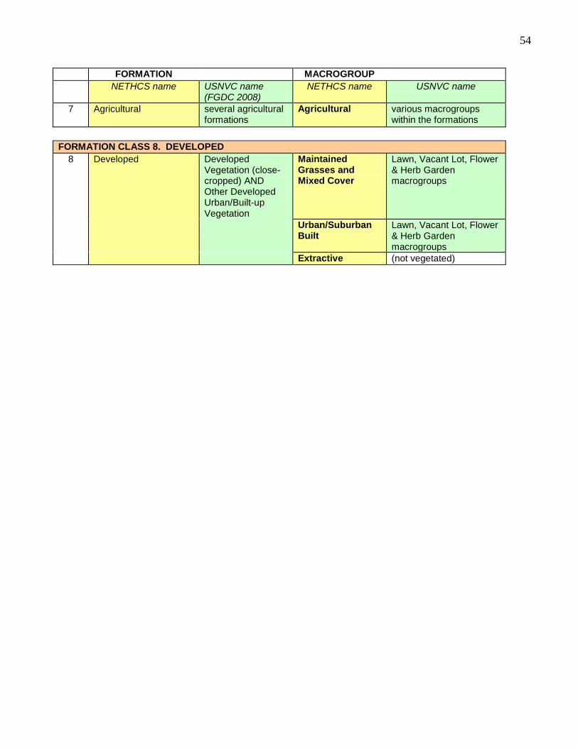
54
FORMATION MACROGROUP
NETHCS name USNVC name (FGDC 2008)
NETHCS name USNVC name
7 Agricultural several agricultural formations
Agricultural various macrogroups within the formations
FORMATION CLASS 8. DEVELOPED
8 Developed Developed Vegetation (close-cropped) AND Other Developed Urban/Built-up Vegetation
Maintained Grasses and Mixed Cover
Lawn, Vacant Lot, Flower & Herb Garden macrogroups
Urban/Suburban Built
Lawn, Vacant Lot, Flower & Herb Garden macrogroups
Extractive (not vegetated)