A ‘‘Vertically Lagrangian’’ Finite-Volume Dynamical … ‘‘Vertically Lagrangian’’...

VOLUME 132 OCTOBER 2004M O N T H L Y W E A T H E R R E V I E W

2293

A ‘‘Vertically Lagrangian’’ Finite-Volume Dynamical Core for Global Models

SHIAN-JIANN LIN

NOAA/Geophysical Fluid Dynamics Laboratory, Princeton University, Princeton, New Jersey

(Manuscript received 7 April 2003, in final form 27 February 2004)

ABSTRACT

A finite-volume dynamical core with a terrain-following Lagrangian control-volume discretization is described.The vertically Lagrangian discretization reduces the dimensionality of the physical problem from three to twowith the resulting dynamical system closely resembling that of the shallow water system. The 2D horizontal-to-Lagrangian-surface transport and dynamical processes are then discretized using the genuinely conservativeflux-form semi-Lagrangian algorithm. Time marching is split-explicit, with large time steps for scalar transport,and small fractional steps for the Lagrangian dynamics, which permits the accurate propagation of fast waves.A mass, momentum, and total energy conserving algorithm is developed for remapping the state variablesperiodically from the floating Lagrangian control-volume to an Eulerian terrain-following coordinate for dealingwith ‘‘physical parameterizations’’ and to prevent severe distortion of the Lagrangian surfaces. Deterministicbaroclinic wave-growth tests and long-term integrations using the Held–Suarez forcing are presented. Impactof the monotonicity constraint is discussed.

1. Introduction

This paper describes the finite-volume dynamical corefor global models that was initially developed at theNational Aeronautics and Space Administration(NASA) Goddard Space Flight Center. The applicationsof the finite-volume algorithms for global modeling atNASA Goddard Space Flight Center (GSFC) started inthe late 1980s and early 1990s with focus on the trans-port process of chemical constituents (e.g., Rood 1987;Allen et al. 1996) and water vapor (Lin et al. 1994).These algorithms were derived and evolved from themodern 1D finite-volume algorithms pioneered by VanLeer (1977) and Colella and Woodward (1984), whichwere originally designed for resolving sharp gradientsand discontinuities in astrophysics and aerospace en-gineering applications.

In addition to the effort at NASA GSFC, finite-vol-ume schemes have also been developed or applied else-where for modeling geophysical flows (e.g., Carpenteret al. 1990, Machenhauer and Olk 1995; Thuburn 1996).The challenge to us was to develop computationallycompetitive and physically based algorithms suitable forglobal modeling of both weather and climate systems.There exists a rich body of literature on high-perfor-mance finite-volume schemes designed for other dis-ciplines (e.g., Roe 1981; Colella and Woodward 1984;Woodward and Colella 1984; Shu and Osher 1988; Har-ten 1989; Huynh 1996; Leveque 2002). However, the

Corresponding author address: Shian-Jiann Lin, NOAA/Geo-physical Fluid Dynamics Laboratory, Forrestal Campus, PrincetonUniversity, Princeton, NJ 08544-0308.E-mail: [email protected]

large-scale atmospheric flow is highly stratified in thedirection of gravitation, and as an excellent approxi-mation, is hydrostatic. As such, the standard ‘‘Riemannsolver’’ developed for other disciplines would not beefficient nor directly applicable. Furthermore, the di-rectional splitting needed for applying the previouslymentioned 1D algorithms would produce unacceptablylarge errors near the poles where the splitting errors aregreatly amplified by the convergence of the meridians(Lin and Rood 1996).

A milestone toward the goal of developing a finite-volume dynamical core was achieved in early 19941 withthe development of the multidimensional Flux-FormSemi-Lagrangian Transport scheme (FFSL; Lin and Rood1996, referred to as LR96 hereafter). Building on theexisting 1D finite-volume schemes, the FFSL algorithmextended those schemes to multidimensions and therebyeliminated the need for directional splitting. Equally im-portant, the so-called Pole-Courant number problem issolved, via the physical consideration of the contributionto fluxes from upstream volumes as far away as the Cour-ant number indicated. The resulting multidimensionalscheme is oscillation free (with the optional monotonicityconstraint), mass conserving, and stable for Courant num-ber greater than one in the longitudinal direction, whichmade the scheme competitive for the intended applicationon the sphere. The FFSL algorithm has since been adopt-ed in several atmospheric chemistry transport models(e.g., Chin et al. 2000; Rotman et al. 2001).

Another milestone toward the goal of building the

1 The multidimensional Flux-Form Transport Algorithm was firstpresented in 1994 at the Fourth Workshop on the Solutions of PartialDifferential Equations on the Sphere and later published in 1996.

2294 VOLUME 132M O N T H L Y W E A T H E R R E V I E W

finite-volume dynamical core was reached with the ad-aptation of the FFSL algorithm to the shallow waterdynamical framework (Lin and Rood 1997, referred toas LR97 hereafter). To achieve the goal of consistenttransport of the mass, the absolute vorticity, and hence,the potential vorticity, a two-grid two-step ‘‘reversedengineering approach’’ was developed. It has the ad-vantage of the Z grid (Randall 1994) without its com-putational expense of solving an elliptic equation. Thetime discretization for treating the gravity waves on bothgrids is the explicit ‘‘forward–backward’’ scheme,which is conditionally stable with the forward-in-timenature of the FFSL transport algorithm. The allowablesize of the time step, for example, for a T42-like res-olution (about 2.88) is 600 s, which is about half of whatcan be used by the semi-implicit Eulerian spectral mod-el. This not-so-small time step made the fully explicitshallow water algorithm computationally competitivewith the spectral and finite-difference methods (e.g.,Bourke 1974; Arakawa and Lamb 1981; Ringler et al.2000).

The final piece needed for the completion of the finite-volume dynamical core was developed after the dis-covery of a simple finite-volume integration method forcomputing the pressure gradient in general terrain-fol-lowing coordinates (Lin 1997, 1998; referred to as L97and L98 hereafter). It is well known that the standardmathematical transformation of the pressure gradientterm in terrain-following coordinates results in twolarge-in-magnitude terms with opposite sign. A straight-forward application of numerical techniques (e.g., cen-ter differencing) to these two terms would typically pro-duce large errors. The finite-volume integration schemeof L97 avoids the mathematical transformation by in-tegrating around the arbitrarily shaped finite volume toaccurately determine the pressure gradient forcing so asto maintain the physical consistency for the finite vol-ume under consideration.

The finite-volume dynamical core developed in L97utilized a sigma vertical coordinate, which requires a3D transport algorithm. Applying the methodology ofLR96, a fully 3D FFSL algorithm would require sixpermutations of 1D operators, instead of two as in 2D.To reduce the computational cost, a simplification wasmade in L97, with some loss in accuracy, to reduce theoperator permutations from six to three, and even downto two (i.e., no cross terms associated with vertical trans-port, as was done in LR96). This computationally mo-tivated simplification is no longer needed after the in-troduction of the Lagrangian control-volume verticaldiscretization (Lin and Rood 1998, 1999) as the di-mensionality of the physical problem is essentially re-duced from three to two, as viewed from the Lagrangiancontrol-volume perspective.

For reference purpose, the full governing equationsfor the atmosphere under the hydrostatic approximationare provided in appendix A using a general verticalcoordinate. Upon the introduction of the Lagrangian

control-volume vertical discretization, all prognosticequations are reduced to 2D, in the sense that they arevertically decoupled. The discretization of the 2D hor-izontal transport process is described in section 2. Thecomplete dynamical system with the Lagrangian con-trol-volume vertical discretization is described in sec-tion 3. A mass, momentum, and total energy conservingremapping algorithm is described in section 4. We pre-sent in section 5, the deterministic baroclinic wavegrowth tests and long-term integrations using the Held–Suarez forcing (Held and Suarez 1994). Concluding re-marks are given in section 6.

2. Discretization of the horizontal transportprocess

We shall follow the equations and notations in ap-pendix A. Since the vertical transport terms vanish withthe Lagrangian control-volume vertical discretization,we present here only the 2D forms of the FFSL algo-rithm for the transport of density and mixing ratio–likequantities. the conservation law for the pseudodensity[Eq. (A3)] reduces to

] 1 ] ]p 1 (up) 1 (yp cosu) 5 0. (1)[ ]]t A cosu ]l ]u

Integrating Eq. (1) analytically in time (for one timestep Dt) and around the finite volume, the previous con-servation law becomes

t1Dt1n11 np 5 p 2 E2A DuDl cosu t

3 p(t ; l, u)V · n dl dt, (2)R[ ]where V(t; l, u) 5 (U, V), dl is the infinitesimal elementalong the volume edges, n is the corresponding outwardnormal vector, is the finite-volume representation ofpp, and the contour integral is taken along the edges ofthe finite volume centered at (l, u).

l1Dl/2 u1Du/21p(t) [ E E2A DuDl cosu

l2Dl/2 u2Du/2

23 p(t; l, u)A cosu du dl. (3)

Equation (2) is still exact. To carry out the contourintegral, certain approximations must be made. LR96effectively decomposed the flux integral using two or-thogonal 1D flux-form transport operators. Introducingthe difference and average operators:

Dx Dxd q 5 q x 1 2 q x 2 ,x 1 2 1 22 2

1 Dx Dxxq 5 q x 1 1 q x 2 ,1 2 1 2[ ]2 2 2

OCTOBER 2004 2295L I N

and assuming (u*, y*) is the time-averaged (from timet to time t 1 Dt) V on the C grid (e.g., Fig. 1 in LR96),the 1-D flux-form transport operator F in the l directionis

t1Dt1F(u*, Dt, p) 5 2 d pU dtl E1 2ADl cosu t

Dt5 2 d [x(u*, Dt; p)] (4)lADl cosu

t1Dt1x(u*, Dt; p) 5 pU dtEDt t

[ u*p*(u*, Dt, p) (5)t1Dt1

p*(u*, Dt; p) ø p dt , (6)EDt t

where x is the time-accumulated (from t to t 1 Dt) massflux across the cell wall, and p* can be interpreted asa time-mean (from time t to time t 1 Dt) pseudodensityvalue of all material that passed through the cell edge.To be exact, the time integration in Eq. (6) should becarried out along the backward-in-time trajectory of thecell-edge position from t 5 t 1 Dt back to time t. Theessence of the 1D finite-volume algorithm is to con-struct, based on the given initial cell-mean values of

, an approximated subgrid distribution of the true ppfield, to enable an analytic integration of Eq. (6). As-suming there is no error in obtaining the time-mean wind(u*), the only error produced by the 1D transport schemewould be solely due to the approximation to the truedistribution of p using the assumed subgrid distribution.From this perspective, it can be said that the 1D finite-volume transport algorithm combined the space–timediscretization in the approximation of the time-meancell-edge value p*. The physically correct way of ap-proximating the integral in Eq. (6) must be ‘‘upwind,’’in the sense that it is integrated along the backwardtrajectory of the cell edges. A center difference ap-proximation to Eq. (6) would be physically incorrect,and consequently numerically unstable without addi-tional numerical damping.

Central to the accuracy and computational efficiencyof the finite-volume algorithms is the degrees of freedomthat describe the subgrid distribution. The first-orderupwind scheme has 0 degree of freedom within the vol-ume as it is assumed that the subgrid distribution ispiecewise constant having the same value everywherewithin the cell as the given volume mean. The second-order finite-volume scheme assumes a piecewise linearsubgrid distribution, which allows 1 degree of freedomfor the specification of the ‘‘slope’’ (or equivalently, the‘‘mismatch’’ as defined by Lin et al. 1994). The piece-wise parabolic method (PPM) has 2 degrees of freedomin the construction of the second-order polynomial with-in the volume, and as a result, the accuracy is signifi-cantly enhanced. The PPM strikes a good balance be-

tween computational efficiency and accuracy. To furtherimprove its accuracy, a modified PPM is presented inappendix B.

While the PPM possesses all the desirable attributes(mass conserving, monotonicity preserving, and high-order accuracy) in 1D, a solution must be found to avoidthe directional splitting for modeling the multidimen-sional dynamics and the transport processes. For 2Dproblems, the first step toward reducing the splittingerror is to apply the two orthogonal 1D flux-form op-erators in a symmetric way. After the directional sym-metry is achieved (by averaging), the ‘‘inner operators’’are then replaced with corresponding advective-formoperators. A consistent advective-form operator ( f ) inthe l direction can be derived from its flux-form coun-terpart (F) as follows:

f (u*, Dt, p) 5 F(u*, Dt, p) 2 pF(u*, Dt, p [ 1)l5 F(u*, Dt, p) 1 pC , (7)def

Dtd u*llC 5 , (8)def ADl cosu

where is a dimensionless number indicating thelCdef

degree of the flow deformation in the l direction. Thepreceding derivation of f is different from LR96’s ap-proach, which adopted the traditional 1D advective-form semi-Lagrangian scheme. The advantage of usingEq. (7) is that computations of winds at cell centers areavoided.

Analogously, 1D flux-form transport operator G inthe latitudinal (u) direction is derived as follows:

t1Dt1G(y*, Dt, p) 5 2 d pV cosu dtu E[ ]ADu cosu t

Dt5 2 d [y*, cosup*] (9)uADu cosu

and likewise the advective-form operator isug(y*, Dt, p) 5 G(y*, Dt, p) 1 pC ,def (10)

where

Dtd (y* cosu)uuC 5 . (11)def ADu cosu

Introducing the following shorthand notations:

1u n n( ) 5 ( ) 1 g[y*, Dt, ( ) ], (12)

2

1l n n( ) 5 ( ) 1 f [u*, Dt, ( ) ], (13)

2

the 2D transport algorithm on the sphere can then bewritten as

n11 n u lp 5 p 1 F(u*, Dt, p ) 1 G(y*, Dt, p ). (14)

Using explicitly the mass fluxes (x, Y), Eq. (14) is re-written as


Dt 1n11 n up 5 p 2 d [x(u*, Dt; p )]l5A cosu Dl

1l1 d [cosuY(y*, Dt; p )] ,u 6Du

(15)

where Y, the mass flux in the meridional direction, isdefined in a similar fashion as x. It can be verified thatin the special case of constant density flow, 5 con-pstant, the preceding equation degenerates to the discreterepresentation of the incompressibility condition of thewind field (u*, y *)

1 1d u* 1 d (y* cosu) 5 0 (16)l uDl Du

The fulfillment of the earlier incompressibility con-dition for constant-density flows is crucial to the ac-curacy of the 2D flux-form formulation. For transportof mixing ratio–like quantities (q) the mass fluxes (x,Y) as defined previously should be used as follows:

1n11 n n u lq 5 [p q 1 F(x, Dt, q ) 1 G(Y, Dt, q )]. (17)

n11p

The preceding form of the tracer transport equationconsistently degenerates to Eq. (15) if q 5 constant,which is another important condition for a flux-formtransport algorithm to be able to avoid generation ofartificial gradients and to maintain mass conservation.

3. The vertically Lagrangian control-volumediscretization

The very idea of using Lagrangian vertical coordinatefor formulating governing equations for the atmosphereis not new. Starr (1945) is the first to formulate thegoverning equations using the Lagrangian coordinateapproach. Starr did not make use of the Lagrangiancontrol-volume concept for discretization nor did he pre-sent a solution to the problem of computing the pressuregradient terms. In the finite-volume discretization, theLagrangian surfaces are treated as the bounding materialsurfaces of the Lagrangian control volumes withinwhich the finite-volume algorithms developed in LR96,LR97, and L97 will be directly applied.

To use a vertical Lagrangian coordinate system, oneshould first address the issue of whether it is an inertialcoordinate or not; for hydrostatic flows, it is. This isbecause both sides of the vertical momentum equationvanish under the hydrostatic assumption. Realizing thatthe earth’s surface, for modeling purpose, is a materialsurface, one can then construct a terrain-following La-grangian control-volume coordinate using the usual ter-rain-following Eulerian coordinate as the starting point.The basic idea is to start the time integration from thechosen terrain-following Eulerian coordinate (e.g., pures or hybrid s-p), treating all initial coordinate surfaces

as material surfaces, the finite volumes bounded by twocoordinate surfaces, that is, the Lagrangian control vol-umes, are free vertically, to float, compress, or expandwith the flow as dictated by the hydrostatic dynamics.

By choosing an imaginary conservative tracer z thatis a monotonic function of height and constant on theinitial coordinate surfaces, the 3D equations written forthe general vertical coordinate in appendix A can bereduced to 2D forms. After factoring out the constantdz, Eq. (A3) in appendix A, the conservation law forthe pseudodensity (p 5 dp/dz ), becomes

] 1 ] ]dp 1 (udp) 1 (ydp cosu) 5 0, (18)[ ]]t A cosu ]l ]u

where the operator d represents the vertical differencebetween the two neighboring Lagrangian surfaces thatbound the finite control-volume. From the hydrostaticbalance, Eq. (A1), the pressure thickness dp of that con-trol volume is proportional to the total mass, that is, dp5 2rgdz. Therefore, it can be said that the Lagrangiancontrol-volume vertical discretization has the hydro-static balance built in.

Similarly, Eq. (A4), the mass conservation law forall tracer species, is

] 1 ] ](qdp) 1 (uqdp) 1 (yqdp cosu) 5 0,[ ]]t A cosu ]l ]u

(19)

the thermodynamic equation, Eq. (A5), becomes

] 1 ] ](Qdp) 1 (uQdp) 1 (yQdp cosu) 5 0,[ ]]t A cosu ]l ]u

(20)

and (A6) and (A7), the momentum equations, are re-duced to

] 1 ] 1 ]u 5 Vy 2 (k 1 f 2 nD) 1 p ,[ ]]t A cosu ]l r ]l

(21)

] 1 ] 1 ]y 5 2Vu 2 (k 1 f 2 nD) 1 p . (22)[ ]]t A ]u r ]u

Given the prescribed pressure at the model top P`,the position of each Lagrangian surface Pl (horizontalsubscripts omitted) is determined in terms of the hy-drostatic pressure as follows:

l

P 5 P 1 dP , (for l 5 1, 2, 3, . . . . , N ),Ol ` kk51

(23)

where the subscript l is the vertical index ranging from1 at the lower bounding Lagrangian surface of the first(the highest) layer to N at the earth’s surface. There areN 1 1 Lagrangian surfaces to define N Lagrangian lay-


ers (here, we use layer interchangeably with controlvolume). The surface pressure, which is the pressure atthe lowest Lagrangian surface, is computed as PN byEq. (23).

With the exception of the pressure-gradient terms andthe addition of a thermodynamic equation, the earlier2D Lagrangian dynamical system is the same as theshallow water system described in LR97. The conser-vation law for the depth of fluid h in the shallow watersystem of LR97 is replaced by Eq. (18) for the pressurethickness dp. The ideal gas law, the mass conservationlaw for air mass, the conservation law for the potentialtemperature, together with the modified momentumequations Eqs. (21) and (22) close the 2D Lagrangiandynamical system, which are vertically coupled only bythe discretized hydrostatic relation.

The time marching procedure for the 2D Lagrangiandynamics follows closely that of the shallow water dy-namics described in LR97. For computational efficien-cy, we take advantage of the stability of the FFSL trans-port algorithm by using a much larger time step (Dt)for the transport of all tracer species (including watervapor). The Lagrangian dynamics uses a relatively smalltime step, Dt 5 Dt/m, where m is the number of thesubcycling needed to stabilize the fastest wave. We de-scribe here a time-split procedure for the prognosticvariables [dp, u, u, y ; q] on the D grid. Discretizationon the C grid for obtaining the diagnostic variables (u*,y *), is analogous to that of the D grid (see LR97).

Introducing the following shorthand notations:

1u n1(i21)/m n1(i21)/m( ) 5 ( ) 1 g[y*, Dt , ( ) ],i i2

1l n1(i21)/m n1(i21)/m( ) 5 ( ) 1 f [u*, Dt, ( ) ]i i2

and applying Eq. (15), the update of ‘‘pressure thick-ness’’ dp, using the fractional time step Dt 5 Dt/m, canbe written for fractional step i 5 1, . . . , m

Dtn1(i /m) n1(i21)/mdp 5 dp 2

A cosu

1u3 d [x*(u*, Dt ; dp )]l i i i5Dl

1l1 d [cosuy*(y*, Dt , dp )] , (24)u i i i 6Du

where ( , ) are the airmass fluxes, which are thenx* y*i i

used as input to Eq. (17) for transport of the potentialtemperature Q.

1n1(i /m) n1(i21)/m n1(i21)/m uQ 5 [dp Q 1 F(x*, Dt ; Q )i in1(i /m)dp

l1 G(y*, Dt , Q )]. (25)i i

With the exception of the pressure-gradient terms, the

discretization of the momentum equations are the sameas those in the shallow water system (LR97).

1n1(i /m) n1(i21)/m lu 5 u 1 Dt y*(y*, Dt ; V ) 2 di i l[ AD cosu

3 (k* 2 nD*) 1 P , (26)l]n1(i /m) n1(i21)/m uy 5 y 2 Dt x*(u*, Dt ; V )i i[

1 1 d (k* 2 nD*) 2 P ,u u]ADu

(27)

where k* and D*, both defined at the corners of the cell(grid), are discretized as

1 un1(i21)/mk* 5 [x*(u* , Dt ; u )i i2

ln1(i21)/m1 y*(y* , Dt ; y )],i i

1 1 1n1(i21)/m n1(i21)/mD* 5 d u 1 d (y cosu) .l u[ ]A cosu Dl Du

The finite-volume mean pressure-gradient terms in Eqs.(26) and (27) are computed as

f dP f dPR RPsl Psu P 5 , P 5 ,l u

A cosu P dl A P duR RPsl Psu

(28)

where P 5 pk (k 5 R/Cp), and the symbols ‘‘P s l’’and ‘‘P s u’’ indicate that the contour integrations areto be carried out, using the finite-volume integrationmethod described in L97, in the (P, l) and (P, u) space,respectively.

Mass fluxes (x*, y*) and the winds (u*, y*) on the Cgrid are accumulated for the large time step transportof tracer species (including water vapor) q.

1n11 n n u lq 5 [q dp 1 F(X*, Dt, q ) 1 G(Y*, Dt, q )],

n11dp(29)

where the time-accumulated mass fluxes (X*, Y*) arecomputed as

m m

u lX* 5 x*(u*, Dt , dp ), Y* 5 y*(y*, Dt , dp ).O Oi i i i i ii51 i51

(30)

The time-averaged winds (U*, V*), to be used as input forthe computations of ql and qu, are defined as follows:


FIG. 1. (Top) Zonal mean wind and (bottom) the derived balancedtemperature.

m m1 1U* 5 u*, V* 5 y*. (31)O Oi im mi51 i51

To complete one full time step, Eqs. (24)–(27), togetherwith their counterparts on the C grid are cycled m timesusing the fractional time step Dt, which are followedby the tracer transport using Eq. (29) with the large timestep Dt. The use of the time-accumulated mass fluxesand the time-averaged winds for the large time steptracer transport ensures the conservation of the tracermass and maintains the highest degree of consistencypossible under the time split integration procedure.

There is formally no Courant number–related timestep restriction associated with the transport processes.There is, however, a stability condition imposed by thegravity wave processes. For application on the wholesphere, it is computationally advantageous to apply ahigh-latitude zonal filter to allow a dramatic increase ofthe size of the small time step Dt. The effect of thezonal filter is to stabilize the short-in-wavelength (andhigh-in-frequency) gravity waves that are being unnec-essarily and undirectionally resolved at very high lati-tudes in the zonal direction. To minimize the impact tometeorologically significant larger-scale waves, the zon-al filter is highly scale selective and is applied only tothe diagnostic variables on the auxiliary C grid and thetendency terms in the D grid momentum equations. Nozonal filter is applied directly to any of the prognosticvariables. Due to the two-grid approach and the stabilityof the FFSL transport scheme, the maximum size of thesmall time step is about 2 to 3 times larger than a modelbased on Arakawa and Lamb’s scheme on the C grid.It is possible to avoid the use of the zonal filter if, forexample, the ‘‘Cubed Sphere grid’’ (Sadourny 1972;Ronchi et al. 1996) is chosen. However, this would re-quire a significant rewrite of the model codes includingphysics parameterizations, the land model, and most ofthe postprocessing packages.

The size of the small time step for the Lagrangiandynamics is only a function of the horizontal resolution.Applying the zonal filter, for the 28 horizontal resolution,a small time step size of 450 s can be used for theLagrangian dynamics. From the large time step transportperspective, the small time step integration of the 2DLagrangian dynamics can be regarded as a very accurateiterative solver, with m iterations, for computing thetime-mean winds and the mass fluxes, analogous infunctionality to a semi-implicit algorithm’s elliptic solv-er (e.g., Ringler et al. 2000). Besides accuracy, the meritof an explicit versus semi-implicit algorithm ultimatelydepends on the computational efficiency of each ap-proach. In light of the advantage of the explicit algo-rithm in parallelization, we do not regard the explicitalgorithm for the Lagrangian dynamics as an impedanceto computational efficiency.

4. A mass, momentum, and total energyconserving remapping algorithm

The Lagrangian surfaces that vertically bound the fi-nite volumes will eventually deform, particularly in thepresence of persistent diabatic heating/cooling, in thetime scale of a few hours to a day depending on thestrength of the heating and cooling, to a degree that itwill negatively impact the accuracy of the horizontal-to-Lagrangian-surface transport and the computation ofthe pressure-gradient terms. Therefore, a key to the suc-cess of the Lagrangian control-volume discretization isan accurate and conservative algorithm for remappingthe deformed Lagrangian coordinate back to a fixed Eu-lerian coordinate.

There are some degrees of freedom in the design ofthe remapping algorithm. To ensure conservation, theremapping algorithm is based on the reconstruction ofthe zonal and meridional ‘‘winds,’’ ‘‘tracer mixing ra-tios,’’ and ‘‘total energy’’ (volume-integrated sum of theinternal, potential, and kinetic energy), using the mono-tonic piecewise parabolic subgrid distributions with the


FIG. 2. The surface pressure perturbation and the temperature at the lowest model layer at day 10 for (top tobottom) three different horizontal resolutions.

hydrostatic pressure as defined by Eq. (23) as the re-mapping coordinate. We outline the remapping proce-dure as follows:

Step 1: Define a suitable Eulerian reference coordi-nate. The surface pressure typically plays an ‘‘an-

choring’’ role in defining the terrain-following Eu-lerian vertical coordinate. The mass in each layer(dp) is then computed according to the chosen Eu-lerian coordinate.

Step 2: Construct vertical subgrid profiles of tracermixing ratios (q), zonal and meridional winds (u,


FIG. 3. The 1000-day average of (upper-left) zonal mean wind, (upper-right) meridional wind, (lower-left) temperatureand (lower-right) vertical pressure velocity simulated with the Held–Suarez forcing at the 28 3 2.58 resolution(B32).

y), and total energy (G) in the Lagrangian control-volume coordinate based on the piecewise para-bolic method. The total energy G is computed asthe sum of the finite-volume integrated geopoten-tial f, internal energy (CyT), and the kinetic energy(K):

1 12 2G 5 C T 1 f 1 (u 1 y ) dp. (32)E y[ ]dp 2

Applying integration by parts and the ideal gas law,the earlier integral can be carried out as

1G 5 C T 1 d(pf) 1 K, (33)p dp

where is the layer mean temperature, K is theTkinetic energy, p is the pressure at layer edges, andCy and Cp are the specific heat of the air at constantvolume and at constant pressure, respectively. Lay-er mean values of [q, (u, y), and G] in the Euleriancoordinate system are obtained by integrating an-alytically the subgrid distributions, in the verticaldirection, from model top to the surface, layer bylayer. Since the hydrostatic pressure is chosen asthe remapping coordinate, air and tracer mass, mo-mentum, and total energy are conserved.

To convert the potential temperature Q to the layermean temperature the conversion factor is obtainedby equating the following two equivalent forms ofthe hydrostatic relation:

df 5 2C QdP, (34)p

df 5 2RTd ln p, (35)

where P 5 pk. The conversion formula betweenlayer mean temperature and layer mean potentialtemperature is

d ln pQ 5 k T. (36)

dP

Step 3: Compute kinetic energy in the Eulerian co-ordinate system for each layer. Substituting kineticenergy and the hydrostatic relationship Eq. (35)into (33), the layer mean temperature for layer kin the Eulerian coordinate is then retrieved fromthe reconstructed total energy (done in step 2) bya fully explicit integration procedure starting fromthe surface up to the model top as follows:

G 2 K 2 fk k k1(1/2)T 5 (37)k

ln p 2 ln pk1(1/2) k2(1/2)C 1 2 kpp k2(1/2)[ ]p 2 pk1(1/2) k2(1/2)


FIG. 4. As in Fig. 3 but for the 18 3 1.258 resolution (C32).

The physical implication of retrieving the layer meantemperature from the total energy is that the dissipatedkinetic energy, if any, is locally converted into internalenergy via the vertically subgrid mixing (dissipation)processes. Due to the monotonicity-preserving natureof the subgrid reconstruction the column-integrated ki-netic energy inevitably decreases (dissipates), whichleads to local frictional heating. The frictional heatingis a physical process that maintains the conservation ofthe total energy in a closed system.

As viewed by an observer riding on the Lagrangiansurfaces, the remapping procedure essentially performsthe physical function of the relative-to-the-Eulerian-co-ordinate vertical transport, by vertically redistributingmass, momentum, and total energy from the Lagrangiancontrol volume back to the Eulerian framework. Theremapping time step can be much larger than that usedfor the large time step tracer transport. In tests usingthe Held–Suarez forcing, a 3-h remapping time intervalis found to be adequate. In the full model integration,one may choose the same time step used for the physicalparameterizations so as to ensure the input to physicalparameterizations are in the usual ‘‘Eulerian’’ verticalcoordinate.

5. Idealized testsWe present results from two types of idealized tests.

The first is a deterministic initial-value-problem test

case illustrating the growth and propagation of baro-clinic instability initiated by a localized perturbation.The second is the ‘‘climate’’ simulation using the Held–Suarez forcing. For both tests we used a 32-level hybrids–p vertical coordinate as the Eulerian coordinate forthe remapping procedure. Below 500 mb, this 32-levelsetup is the same as the National Center for AtmosphericResearch (NCAR) Community Climate Model(CCM3)’s 18-level setup for climate simulations (Kiehlet al. 1996). To better resolve the stratosphere, the ver-tical resolution is substantially increased (as comparedto CCM3) near and above the tropopause level. Themodel top is located at 0.4 mb.

The initial condition for the baroclinic instability testcase is specified analytically as

2 4U(u, p) 5 U ze(z /4) sin (2u),o (38)

where z 5 log(p0/p), Po 5 1000 (mb), Uo 5 35 m s21.The mean flow, which is symmetric with respect to theequator, is in hydrostatic equilibrium with the meridi-onal wind being identically 0. The balanced zonal meantemperature is then computed numerically. The basestate thus constructed is a steady-state solution to the3D governing equations. To break the symmetry and totrigger the growth of the baroclinic instability, a local-ized initial temperature perturbation centered at 458Nand 908E is superimposed to the mean field. Previoustheoretical studies (e.g., Lin and Pierrehumbert 1993)


indicated that the localized disturbance will propagateeastward while growing exponentially. Due to nonlin-earity and periodicity of the spherical geometry, theinstability will saturate and the perturbation will cyclezonally to become a global mode.

Figure 1 depicts the prescribed zonal mean wind andthe derived balanced temperature. The wind is a fairlyrealistic representation of the annual-mean conditionwith the derived temperature showing a cold tropicaltropopause centered near 100 mb and with realistic lapserates throughout the globe. Experiments were carriedout using three progressively higher horizontal resolu-tions: one at 28 3 2.58 (denoted as B32), the second at18 3 1.258 (denoted as C32), and the third at 0.58 30.6258 (denoted as D32), with small time steps of 450,225, and 112.5 s, respectively. The remapping time stepis fixed to be 1 h for all presented tests.

Figure 2 compares, at day 10, the surface pressureperturbations and the temperature at the model’s lowestlayer. It is seen that the phases of the propagation ofthe disturbances agree remarkably well among all threeresolutions. However, the amplitudes in the lower-res-olution runs are somewhat weaker. These are expectedcharacteristics of the monotonicity-preserving finite-volume algorithms. The initial-value problem tests pro-vided no proof that the simulations are ‘‘correct’’ orhave converged. In fact, the results show that even atapproximately 55-km resolution the detailed features ofthe cyclones may still be underresolved. Nevertheless,a reasonable degree of convergence, particularly thelarge-scale features, has been achieved, and there is nopathological amplification of the numerical noise in anyresolutions we tested. While a monotonicity-preservingalgorithm is beneficial to scalar transport, its advantageis unclear in climate simulations in which the preser-vation of variances is regarded as more important. Thisissue is examined using the Held–Suarez forcing.

We applied the same initial condition used in the ear-lier tests to initialize the Held–Suarez test. The inte-grations were carried out for more than 4 yr. Statisticswere computed only for the last 1000 days. Figure 3and Fig. 4 show, respectively, for the B32 and C32resolutions, the zonal mean u-wind, y-wind, tempera-ture, and the vertical pressure velocity.

Within the Lagrangian framework, the vertical pres-sure velocity is diagnosed as follows:

t1Dt tdp p 2 pk k k5 ,dt Dt

where the subscript k indicates the kth Lagrangian sur-face; is the pressure of the kth Lagrangian surfacet1Dtpk

at time t 1 Dt before remapping (Lagrangian coordi-nate), is the value at time t immediately after thetpk

previous remapping (Eulerian coordinate), and Dt is theremapping time step.

The simulated zonal mean fields are in good agree-ment with Held and Suarez’s results. In particular, there

is a distinct ‘‘tropical tropopause’’ of about 190 K, andthere is also a cold surface layer. The simulated zonalmean flows are not exactly symmetric with respect tothe equator due to the asymmetric initial perturbationand the limited averaging period. There are subtle dif-ferences between the two resolutions. Most notably thetropical tropopause in the higher C32 resolution is a bitcolder than that from the B32 case whereas the polar‘‘tropopause’’ (not clearly defined, but roughly at the250-mb level) in the C32 is slightly warmer. The warm-ing of the polar tropopause with increasing horizontalresolution is consistent with full physics simulationsusing the CCM3 parameterizations (to be presented else-where).

Figure 5 (for B32 case) and Fig. 6 (for C32 case)show the eddy momentum transport, eddy heat trans-port, zonal wind variance, and the temperature variance.Except for the zonal wind variance, a good degree ofconvergence has been achieved between the two reso-lutions. However, the differences with Held–Suarez’sresults were more pronounced in the second-momentstatistics. For example, the temperature variances in oursimulations show only a single maxima in the uppertroposphere of the midlatitudes whereas in the Held andSuzrez’s results there is a secondary maxima, whichcould be of numerical origin.

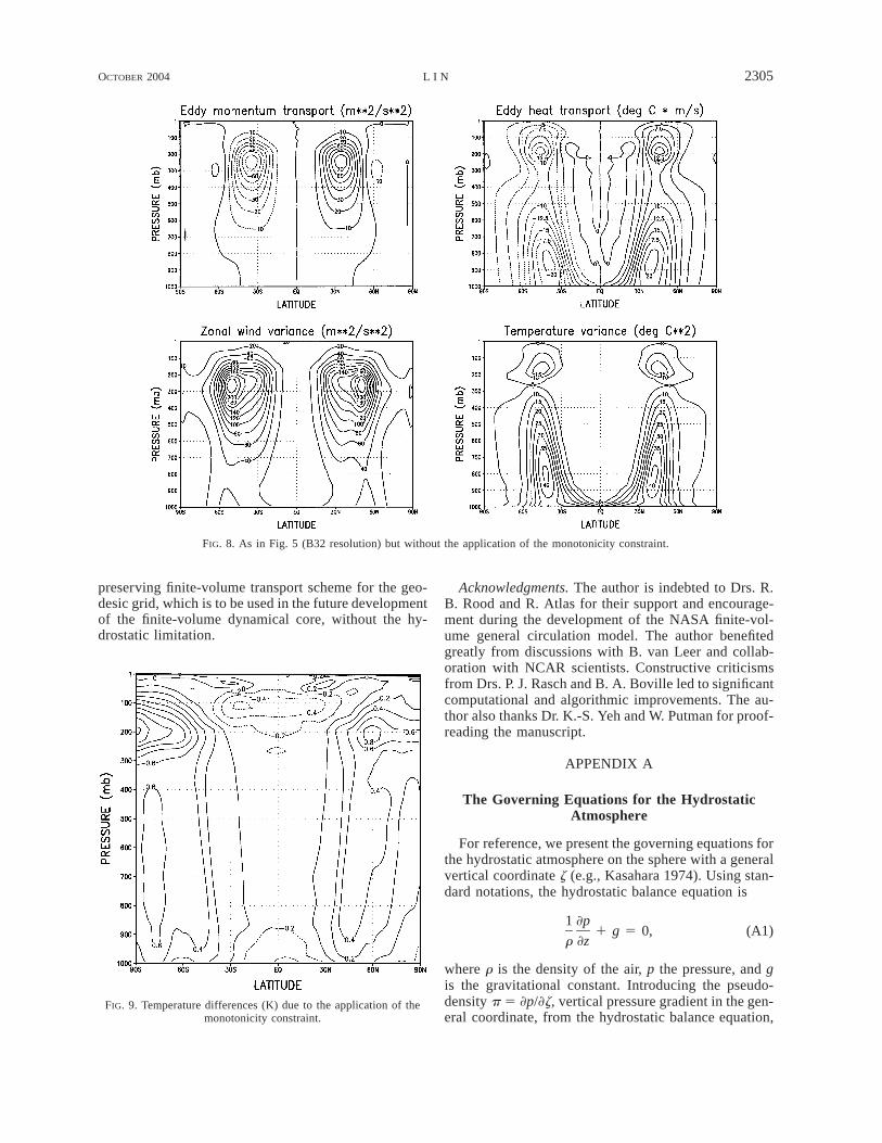
To examine the impacts of monotonicity constraint,which damps strongly the two-grid-scale structures, tothe simulated climate, we carried out another experimentwith the B32 resolution but without applying the mono-tonicity constraint to all horizontal transport processes.Figures 7 and 8 show, respectively, the mean states andthe eddy statistics. It is seen that without the monoto-nicity constraint the simulation is, not surprisingly, clos-er to the higher-resolution (C32) case.

Figure 9 shows the differences in zonal mean tem-perature due to the monotonicity constraint. It indicatesthat, without the monotonicity constraint, poleward heattransport is more rigorous, resulting in warmer polesand cooler Tropics. The monotonicity constraint’s seem-ingly negative impact to ‘‘climate simulations’’ needsto be reexamined in full model simulations, which isbeyond the scope of this paper. It should be noted thatthe monotonicity constraint is highly desirable for thetransport of water vapor, cloud water, and chemical trac-ers to prevent the generation of negative values. In short-term deterministic initial-value problems (e.g., weatherpredictions), it can be argued that elimination of grid-scale numerical noise is more important than the main-tenance of variances. On the other hand, it may be moreimportant to preserve the variances in long-term climatesimulations.

6. Concluding remarks

The finite-volume dynamical core described here hasbeen successfully implemented into two general circu-lation modeling systems, the NASA–NCAR general cir-


FIG. 5. The 1000-day average of eddy statistics: (upper-left) eddy momentum transport, (upper-right) heat transport,(lower-left) zonal wind variance, and (lower-right) temperature variance simulated with the Held–Suarez forcing at the28 3 2.58 resolution (B32).

culation model (fvGCM, to be described elsewhere) andthe Community Atmosphere Model (CAM). It is alsoin the process of being implemented into GeophysicalFluid Dynamics Laboratory’s Flexible Modeling System(FMS) for climate applications. At the NASA Data As-similation Office (DAO), we have already successfullyintegrated the fvGCM into a new generation of the dataassimilation system: the finite-volume Data Assimila-tion System (fvDAS). Numerical weather prediction ex-periments using the fvGCM with initial conditions pro-duced by fvDAS indicated there is significant improve-ment in the forecast skill over DAO’s previous opera-tional system [Goddard Earth Observing System(GEOS-3) DAS].

There are still some aspects of the numerical for-mulation in this dynamical core that can be further im-proved. For example, the choice of the horizontal grid,the computational efficiency of the split-explicit timemarching scheme, the application of the various mono-tonicity constraints, and how the conservation of thetotal energy is achieved. The vertical Lagrangian dis-cretization with the associated remapping conserves thetotal energy exactly. The only remaining issue regardingthe conservation of the total energy is the use of theapparently ‘‘diffusive’’ monotonicity-preserving trans-port scheme for the horizontal discretization.

The full impact of the nonlinear diffusion associatedwith the monotonicity constraint is difficult to access.All discrete schemes must address the problem of sub-grid-scale mixing. The nonlinear diffusion in the finite-volume scheme creates strong local mixing when mono-tonicity principles are violated. However, this local mix-ing diminishes quickly as the resolution matches betterto the spatial structure of the flow. In other numericalschemes, however, an explicit (and tunable) linear dif-fusion is often added to the equations to provide thesubgrid-scale mixing as well as to smooth and/or sta-bilize the time marching.

To compensate for the loss of total energy due tohorizontal discretization, one could apply a global fixerto add the loss in kinetic energy due to ‘‘diffusion’’back to the thermodynamic equation so that the totalenergy is conserved. However, our experience showsthat even without the ‘‘energy fixer’’ the loss in totalenergy (in flux unit) in a full GCM simulation is lessthan 2 (W m22) with the 28 resolution, and much smallerwith higher resolutions. Alternatively, one could con-sider using the total energy as a prognostic variable sothat the total energy could be automatically conserved.

Extension of the algorithms described in this paperto unstructured grids is possible but not straightforward.We are currently developing a high-order monotonicity-


FIG. 6. As in Fig. 5 but for the 18 3 1.258 resolution (C32).

FIG. 7. As in Fig. 3 (B32 resolution) but without the application of the monotonicity constraint.


FIG. 8. As in Fig. 5 (B32 resolution) but without the application of the monotonicity constraint.

FIG. 9. Temperature differences (K) due to the application of themonotonicity constraint.

preserving finite-volume transport scheme for the geo-desic grid, which is to be used in the future developmentof the finite-volume dynamical core, without the hy-drostatic limitation.

Acknowledgments. The author is indebted to Drs. R.B. Rood and R. Atlas for their support and encourage-ment during the development of the NASA finite-vol-ume general circulation model. The author benefitedgreatly from discussions with B. van Leer and collab-oration with NCAR scientists. Constructive criticismsfrom Drs. P. J. Rasch and B. A. Boville led to significantcomputational and algorithmic improvements. The au-thor also thanks Dr. K.-S. Yeh and W. Putman for proof-reading the manuscript.

APPENDIX A

The Governing Equations for the HydrostaticAtmosphere

For reference, we present the governing equations forthe hydrostatic atmosphere on the sphere with a generalvertical coordinate z (e.g., Kasahara 1974). Using stan-dard notations, the hydrostatic balance equation is

1 ]p1 g 5 0, (A1)

r ]z

where r is the density of the air, p the pressure, and gis the gravitational constant. Introducing the pseudo-density p 5 ]p/]z, vertical pressure gradient in the gen-eral coordinate, from the hydrostatic balance equation,


the pseudodensity and the true density are related asfollows:

]fp 5 2 r, (A2)

]z

where f 5 gz is the geopotential. Note that p reducesto the true density if z 5 2gz, and the surface pressurePs if z 5 s(s 5 p/Ps). The conservation of total airmass using p as the prognostic variable can be written as

]p 1 = · (Vp) 5 0, (A3)

]t

where V 5 (u, y, dz/dt). Similarly, the mass conservationlaw for tracers (or water vapor) can be written as

](pq) 1 = · (Vpq) 5 0, (A4)

]t

where q is the mass mixing ratio (or specific humidity)of the tracers (or water vapor). Choosing the potentialtemperature Q as the thermodynamic variable, the firstlaw of thermodynamics can be formulated as

](p Q) 1 = · (Vp Q) 5 0. (A5)

]t

Let (l, u) denote the (longitude, latitude) coordinate,the momentum equations are written in the ‘‘vector-invariant form’’ (e.g., Arakawa and Lamb 1981)

] 1 ] 1 ]u 5 Vy 2 (k 1 f 2 nD) 1 p)[ ]]t A cosu ]t r ]l

dz ]u2 , (A6)

dt ]z

] 1 ] 1 ] dz ]yy 5 2Vu 2 (k 1 f 2 nD) 1 p 2 ,[ ]]t A ]u r ]u dt ]z

(A7)

where A is the radius of the earth, n is the coefficientfor the optional divergence damping, D is the horizontaldivergence, V is the vertical component of the absolutevorticity, k is the kinetic energy, f is the geopotential,and v is the angular velocity of the earth:

1 ] ] 12 2D 5 (u) 1 (y cosu) , k 5 (u 1 y ),[ ]A cosu ]l ]u 2

1 ] ]V 5 2v sinu 1 y 2 (u cosu) .[ ]A cosu ]l ]u

Note that the last term in Eqs. (A6) and (A7) vanishesif z is a conservative quantity [e.g., entropy under adi-abatic condition (e.g., Hsu and Arakawa 1990) or animaginary conservative tracer (see section 3)], and the3D divergence operator becomes 2D along constant zsurfaces.

APPENDIX B

Relaxed Monotonicity Constraints for PPM

The original PPM as described by Colella and Wood-ward (1984) has been modified to improve its compu-tational performance and to reduce the numerical dif-fusion. The PPM is built on the second-order Van Leerscheme. Given the cell-mean value qi and assuming uni-form grid spacing, the ‘‘mismatch’’ (Lin et al. 1994) ofthe piecewise linear distribution is determined as

monoDq i (B1)min min max5 sign[min (|Dq | , Dq , Dq ), Dq ],i i i i

where

1Dq 5 (q 2 q )i i11 i214

maxDq 5 max (q , qi, q ) 2 q ,i i21 i11 i

minDq 5 q 2 min (q , q , q ).i i i21 i i11

In the preceding equations and the rest of the appen-dix the functions sign, min, and max are as defined inthe Fortran language. To uniquely determine a parabolicpolynomial within the finite volume, in addition to thevolume mean value, the values at both edges of theparabola must be determined. The first guess value atthe left edge of the piecewise parabolic distribution iscomputed as

1 12 mnoo monoq 5 (q 1 q ) 1 (Dq 2 Dq ). (B2)i i21 i i21 i2 3

By continuity, the right-edge value of cell (i) is simplythe left-edge value of cell (i 1 1). That is, 5 .1 2q qi i11

The application of a monotonicity constraint breaks thecontinuity of the subgrid distribution between the cells.In the current implementation, different constraints areused in the horizontal and vertical directions. For thehorizontal direction, the first guess edge values as com-puted by Eq. (B2) are adjusted as follows:

2 mono 2 monoq ← q 2 sign[min (|2Dq | , |q 2 q | ), 2Dq ],i i i i i i

(B3)1 mono 1 monoq ← q 1 sign[min (|2Dq | , |q 2 q | ), 2Dq ].i i i i i i

(B4)

The previous constraint produces less diffusive resultsand is much simpler than the original PPM. To furtherreduce the implicit damping, an even less diffusive butmore complicated quasi-monotonic constraint is usedfor the vertical remapping of the moisture and all tracers.The following constraint is based on the improvedwave-resolution scheme of Huynh (Huynh 1996).

Left (top) edge:2 2 min maxq ← min[max(q , q ), q ],i i i i (B5)

where


min mp lc max mp cq 5 min (q , q , q ), q 5 max (q , q , q ),i i i i i i i i

mp monoq 5 q 2 2Dq ,i i i

3lc mono mon monoq 5 q 1 (Dq 2 Dq ) 2 Dq .i i i12 i i2

Right (bottom) edge:1 1 min maxq ← min[max(q , q ), q ],i i i i (B6)

wheremin mp lc max mp cq 5 min (q , q , q ), q 5 max (q , q , q ),i i i i i i i i

mp monoq 5 q 1 2Dq ,i i i

3lc mono mon monoq 5 q 1 (Dq 2 Dq ) 1 Dq .i i i i22 i2

After the application of one of the constraints, the‘‘curvature’’ of the parabola is computed using the meanand the two edge values as

12 1q 0 5 6 q 2 (q 1 q ) . (B7)i i i i[ ]2

REFERENCES

Allen, D. J., P. J. Kasibhatla, A. M. Thompson, R. B. Rood, B. G.Doddridge, K. E. Pickering, R. D. Hudson, and S.-J. Lin, 1996:Transport induced interannual variability of carbon monoxidedetermined using a chemistry and transport model. J. Geophys.Res., 101, 28 655–28 669.

Arakawa, A., and V. R. Lamb, 1981: A potential enstrophy and energyconserving scheme for the shallow-water equations. Mon. Wea.Rev., 109, 18–36.

Bourke, W., 1974: A multilevel spectral model. I. Formulation andhemispheric integration. Mon. Wea. Rev., 102, 687–701.

Carpenter, R. L., K. K. Drogemeier, P. R. Woodward, and C. E. Hane,1990: Application of the piecewise parabolic method to mete-orological modeling. Mon. Wea. Rev., 118, 586–612.

Chin, M., R. B. Rood, S.-J. Lin, J.-F. Muller, and A. M. Thompson,2000: Atmospheric sulfur cycle simulation in the global modelGOCART: Model description and global properties. J. Geophys.Res., 105, 24 671–24 687.

Colella, P., and P. R. Woodward, 1984: The piecewise parabolic meth-od (PPM) for gasdynamical simulations. J. Comput. Phys., 54,174–201.

Harten, A., 1989: ENO schemes with subcell resolution. J. Comput.Phys., 83, 148–184.

Held, I. M., and M. J. Suarez, 1994: A proposal for the intercom-parison of the dynamical cores of atmospheric general circulationmodels. Bull. Amer. Meteor. Soc., 75, 1825–1830.

Hsu, Y.-J. G., and A. Arakawa, 1990: Numerical modeling of theatmosphere with an isentropic vertical coordinate. Mon. Wea.Rev., 118, 1933–1959.

Huynh, H. T., 1996: Schemes and constraints for advection. Proc.Fifth Int. Conf. on Numerical Methods in Fluid Dynamics, Mon-terey, CA.

Kasahara, A., 1974: Various vertical coordinate systems used fornumerical weather prediction. Mon.Wea. Rev., 102, 504–522.

Kiehl, J. T., J. J. Hack, G. B. Bonan, B. A. Boville, B. P. Briegleb,

D. L. Williamson, and P. J. Rasch, 1996: Description of theNCAR Community Climate Model (CCM3). NCAR Tech. Note.NCAR/TN-4201STR, Boulder, CO, 152 pp.

Leveque, R. J., 2002: Finite Volume Methods for Hyperbolic Prob-lems. Cambridge University Press, 558 pp.

Lin, S.-J., 1997: A finite-volume integration method for computingpressure gradient forces in general vertical coordinates. Quart.J. Roy. Meteor. Soc., 123, 1749–1762.

——, 1998: Reply to comments by T. Janjic on ‘‘A finite-volumeintegration method for computing pressure gradient forces ingeneral terrain-following coordinates.’’ Quart. J. Roy. Meteor.Soc., 124, 2531–2533.

——, and R. T. Pierrehumbert, 1993: Is the midlatitude zonal flowabsolutely unstable? J. Atmos. Sci., 50, 1282–1297.

——, and R. B. Rood, 1996: Multidimensional flux form semi-La-grangian transport schemes. Mon. Wea. Rev., 124, 2046–2070.

——, and ——, 1997: An explicit flux-form semi-Lagrangian shallowwater model on the sphere. Quart. J. Roy. Meteor. Soc., 123,2477–2498.

——, and ——, 1998: A flux-form semi-Lagrangian general circu-lation model with a Lagrangian control-volume vertical coor-dinate. Proc. the Rossby-100 Symp., Stockholm, Sweden, Uni-versity of Stockholm, Sweden, 220–222.

——, and ——, 1999: Development of the joint NASA/NCAR Gen-eral Circulation Model. Preprints, 13th Conf. on NumericalWeather Prediction, Denver, CO, Amer. Meteor. Soc., 115–119.

——, W. C. Chao, Y. C. Sud, and G. K. Walker, 1994: A class ofthe van Leer–type transport schemes and its applications to themoisture transport in a general circulation model. Mon. Wea.Rev., 122, 1575–1593.

Machenhauer, B., and M. Olk, 1996: On the development of a cell-integrated semi-Lagrangian shallow water model on the sphere.Proc. ECMWF Workshop on Semi-Lagrangian Methods, Read-ing, United Kingdom, ECMWF, 213–228.

Randall, D. A., 1994: Geostrophic adjustment and the finite-differ-ence shallow-water equations. Mon. Wea. Rev., 122, 1371–1377.

Ringler, T. D., R. P. Heikes, and D. A. Randall, 2000: Modeling theatmospheric general circulation using a spherical geodesic grid:A new class of dynamical cores. Mon. Wea. Rev., 128, 2471–2490.

Roe, P. L., 1981: Approximate Riemann solvers, parameter vectors,and difference schemes. J. Comput. Phys., 43, 357–372.

Ronchi, C., R. Iacono, and P. S. Paolucci, 1996: The ‘‘Cubed Sphere:’’A new method for the solution of partial differential equationsin spherical geometry. J. Comput. Phys., 124, 93–114.

Rood, R. B., 1987: Numerical advection algorithms and their role inatmospheric transport and chemistry models. Rev. Geophys., 25,71–100.

Rotman, D., and Coauthors, 2001: Global Modeling Initiative As-sessment Model: Model description, integration and testing ofthe transport shell. J. Geophys. Res., 106 (D2), 1669–1691.

Sadourny, R., 1972: Conservative finite-difference approximations ofthe primitive equations on quasi-uniform spherical grids. Mon.Wea. Rev., 100, 136–144.

Shu, C.-W., and S. Osher, 1988: Efficient implementation of essen-tially non-oscillatory schemes. J. Comput. Phys., 77, 439–471.

Starr, V. P., 1945: A quasi-Lagrangian system of hydrodynamicalequations. J. Meteor., 2, 227–237.

Thuburn, J., 1996: Multidimensional flux-limited advection schemes.J. Comput. Phys., 123, 74–83.

Van Leer, B., 1977: Toward the ultimate conservative differencescheme. Part IV: A new approach to numerical convection. J.Comput. Phys., 23, 276–299.

Woodward, P. R., and P. Colella, 1984: The numerical simulation oftwo-dimensional fluid flow with strong shocks. J. Comput. Phys.,54, 115–173.

A ‘‘Vertically Lagrangian’’ Finite-Volume Dynamical … ‘‘Vertically Lagrangian’’...

Documents

Transcript of A ‘‘Vertically Lagrangian’’ Finite-Volume Dynamical … ‘‘Vertically Lagrangian’’...