Recent developments in NWP and climate modelling in Russia

M.Tolstykh, Hydrometcentre of Russia;

Institute of Numerical Matematics Russian Academy of Sciences

WGNE-27, Boulder, 17-21 October 2011

Plan

  Progress in global and regional models   Data assimilation   Seasonal forecasts: coupled model   Climate modelling at INM RAS

Short and medium-range numerical weather prediction

  Global models (SL-AV and T169L31)   LAM – COSMO-RU   Global ensemble prediction system– based

on T169 and SL-AV global models   ==================   Computers: SGI ALtix4700 (11 Tflops peak

1664 Itanium2 cores); SGI Ice cluster (1410 cores, 16 Tflops peak)

SL-AV model   Semi-Lagrangian vorticity-divergence dynamical

core of own development, ALADIN/LACE parameterizations.

  Mire parameterization of own development.   Currently, 0.9x0.72 degrees lon/lat, 28 levels, runs

on Altix 4700 computer   Principal global operational model of RHMC   Version with the resolution 0.225x(0.18-0.23)

degrees, 51 levels under testing.   Implemented CLIRAD SW radiation

parameterization, encouraging results in the stratosphere.

  Mass-conserving SL shallow water model on the reduced lat-lon grid – submitted to J.Comput.Phys.

New version o SL-AV model. Grid step (km) in latitude vs latitude

(degrees) (grey)

Plans for SL-AV development

  Testing and tuning with CLIRAD SW radiation parameterization.

  Implementation of 8-level soil (+multilayer snow) parameterization from INM climate model.

  3-D mass conserving semi-Lagrangian advction on the reduced lat-lon grid.

  Plan to run ~20 km version quasioperationally early 2012.

T169L31 model   Spectral dynamical core   Currently, T169, 0.71x0.71 degrees lon/lat,

31 levels, runs on Altix 4700 computer   Secondary operational global model of

Roshydromet   Version T339L31 (0.35x0.35 degrees lon/

lat) is prepared for regular running   The upgraded parameterization scheme of

radiation transfer

LW SW↓

Increase of spectral resolution (old 5, new 8) and new water vapor calculation algorithm allowed to decrease the differences between model and samples by 3-4 times

SW↑

Plans for spectral model development in 2012-2013:

  T339L31: Parallel runs in pre-operational mode   Corrected soil thermal properties and soil

vertical structure   Corrected algorithms for initial data of snow

depth and WE and boundary thermal conditions (OI based)

GME Δx = 30/20 km

COSMO-RU7 Δx = 7 km

COSMO-RU2 Δx =2.2 km Domain: 900 km * 1000 km Grid: 420*470 * 50 Step: 2.2 km Time step: 15 s Forecast: 24 hours Cores: 400

COSMO-RUsib Δx =14 km

GME: initial and boundary data

Domain: 4900 km * 4340 km Grid: 700*620 * 40 Step: 7 km Time step: 40 s Forecast: 78 hours Cores: 800

Domain: 5000 km * 3500 km Grid: 360*250 * 40 Step: 14 km Time step: 80 s Forecast: 78 hours Cores: 48.

10 11/7/11

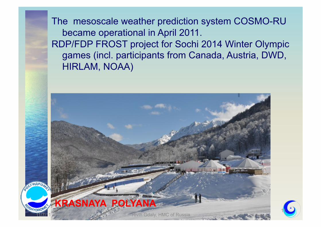
The mesoscale weather prediction system COSMO-RU became operational in April 2011.

RDP/FDP FROST project for Sochi 2014 Winter Olympic games (incl. participants from Canada, Austria, DWD, HIRLAM, NOAA)

11 KRASNAYA POLYANA

11/7/11 Rivin Gdaly, HMC of Russia

• A new EPS version was implemented in February 2011 • Main advantages of the new version: increased resolution and extended output • Now new and old versions run in parallel • Operational trials of the new version start in autumn 2011

Old version: EPS T85L31 New version: EPS T169L31

First implemented April 2008 February 2011

Membership 15 12 perturbed T85L31

3 control: T85L31,T169L31,SLAV-2008

14 12 perturbed T169L31

1 control T169L31 1 control SLAV-2008

Initial data perturbations

Breeding with regional rescaling, 12hr cycling

Runs per day (UTC ) 1 (12 UTC)

Forecast length T+0h -- T+240h at 6 hrs

Input Hydrometcenter of Russia OA 2.5*2.5

Hydrometcenter of Russia OA 1.25*1.25

Computer A four-node computer based on Quad-Core Intel Xeon5345

(2.33 GHz)

SGI Altix 4700 Itanium 2 1.66 GHz, NUMALink, 1664 PEs, Peak 11 Tflops

Output T850,H500,pmsl (2.5*2.5), convective, large-scale, and

total prec (1.25*1.25)

TIGGE-like base (1.25*1.25)

From October 2010: Verification results for precipitation are published on the Web site of the Lead Centre on

Verification of Ensemble Prediction System http://epsv.kishou.go.jp/EPSv/html/rumseps/probdiagrams.html

Data assimilation

  3D-Var-FGAT for global models under quasioperational tuning (M.Tsyrulnikov).

  LETKF for 3D SL-AV global model is being implemented (A.Shlyaeva) following successful testing of the shallow-water version.

M Tsyrulnikov, P Svirenko, V Gorin, M Gorbunov, A Ordin

- first guess: still, 6-h GFS forecast

-  operational tests are underway

-  cyclic DA with the SL-AV global model: under development

-  regional 3D-Var version using stretched geometry: under development

-  Assimilated satellite data: AMSU-A, COSMIC, GRAS, GRACE, AMV-Geo, AMV Polar, AMV-LeoGeo (mixed

geostationary/polar AMV produced by CIMMS), ASCAT

-  Gorin V.E. and Tsyrulnikov M.D. Estimation of multivariate observation- error statistics for AMSU-A data. – Mon. Wea. Rev., 2011 (in print).

3D-Var

3D-Var: Impact of AMSU-A channels 5-10 on 24-h SL-AV forecasts, 20-90N RMS error (w.r.t. an independent analysis).

[Red: without AMSU, Blue: with AMSU.]

(F  is  the  tendency,  mu  random  multiplier)  

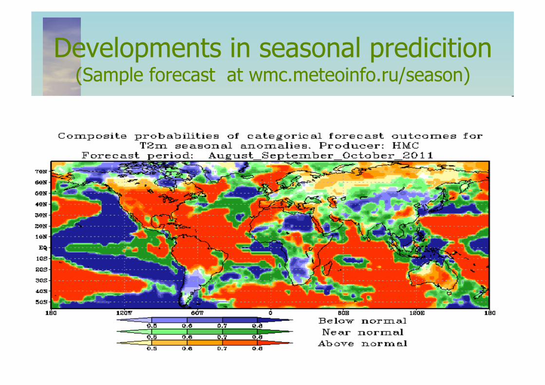
Developments in seasonal predicition (Sample forecast at wmc.meteoinfo.ru/season)

Particular features of the seasonal version of SL-AV model

  Resolution 1.4x1.125 degrees lon/lat, 28 levels. Described in (Tolstykh et al, Izvestia RAN, Ser. PhA&O, 2010)

  Stochastic parameterization of large-scale precipitation (Kostrykin, Ezau, Russian Meteorology and Hydrology, 2001).

  Hybrid deep convection closure (Tolstykh, WGNE Res. Act. 2003)

  Allows to have more realistic precipitation with relatively low resolution.

Further development of the seasonal version of SL-AV model

  Introduction of zonal mean-vertical distribution of ozone instead of vertical profile, tuning.

  Replacement of temperature and soil water content from the reanalysis (+empiric initialization of soil ice) by own data generated with 30 years of assimilation of soil variables (including soil ice) using 2m temperature and RH reanalysis

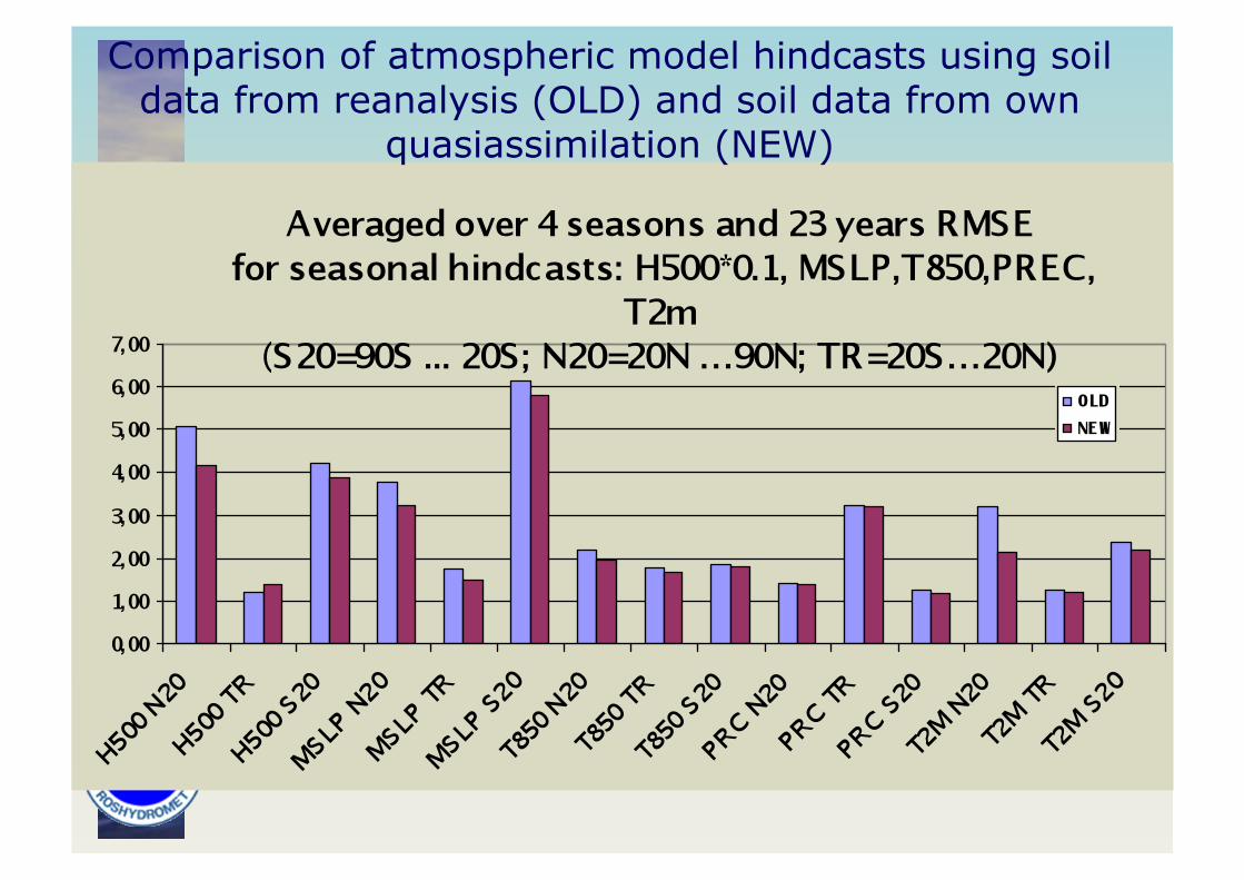
Comparison of atmospheric model hindcasts using soil data from reanalysis (OLD) and soil data from own

quasiassimilation (NEW)

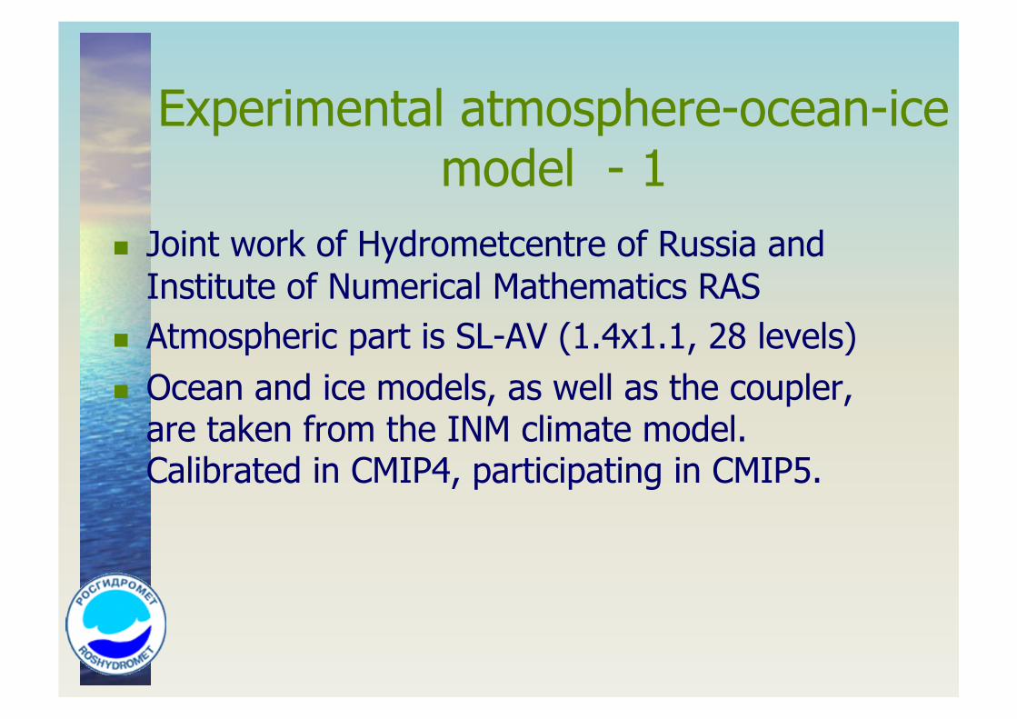
Experimental atmosphere-ocean-ice model - 1

  Joint work of Hydrometcentre of Russia and Institute of Numerical Mathematics RAS

  Atmospheric part is SL-AV (1.4x1.1, 28 levels)   Ocean and ice models, as well as the coupler,

are taken from the INM climate model. Calibrated in CMIP4, participating in CMIP5.

INMOM Ocean model

  Sigma-coordinate model with isopicnic horizontal diffusion

  1˚x0.5˚ , 40 levels   The EVP (elastic- viscous- plastic) dynamics,

Semtner thermodynamics sea ice model (Hunke, Ducowicz 1997; Iakovlev, 2005) is embedded.

  Coupling to the atmospheric model without flux correction

Coupled atmosphere-ocean model for seasonal prediction (2)

  Globally averaged over 4 seasons heat flux to the ocean with one-way interaction is 4.5 W/m2. Model tuning allowed to reduce this value to 2.8 W/m2.

  Atmosphere and ocean models are coupled without flux correction.

  10-member ensemble. Only atmospheric initial data is perturbed.

  Seasonally averaged atmospheric circulation of the coupled model for months 2-4 is compared to the results of atmospheric model with simple SST evolution.

Calculating seasonal hindcasts with the coupled model: Initial data

  Running INMOM ocean model for 1989-2010 using ERA-Interim atmospheric forcing. Archiving ocean model state for the moments when historical seasonal forecasts start

  Using NCEP/NCAR reanalysis-2 data in upper atmosphere + SLP as initial data for atmospheric model.

  For soil variables, using own soil assimilation scheme correcting soil variables from T2m and RH2m 6-hour forecast error. T2m and RH2m analyses still come from reanalysis-2.(Attempts to use soil fields from reanalyses led to bad results!)

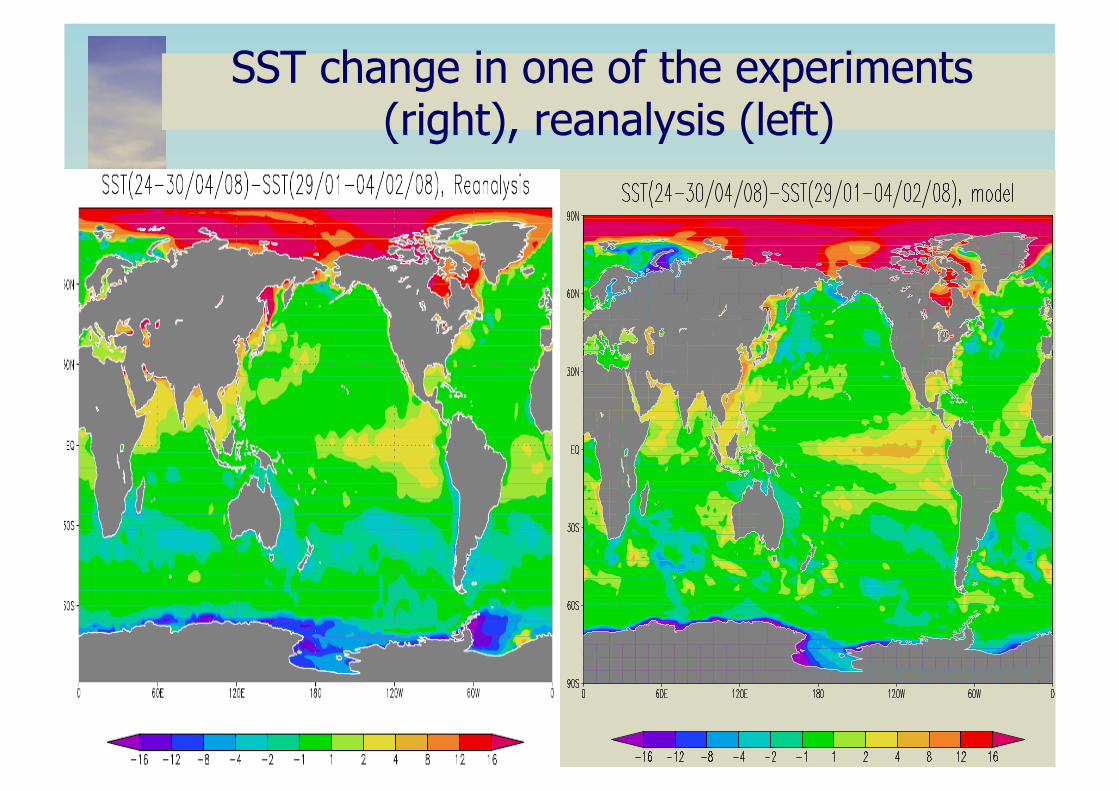
SST change in one of the experiments (right), reanalysis (left)

Errors for 500 hPa height (H500) [м], sea-level pressure (MSLP) [mb], 2m temperature (T2m)[˚C], averaged over 1989-2010 years for all seasons for atmospheric model with SST extrapolation (SLAV) and

coupled model (CM). Full fields and model anomalies (ANOM) SLAV RMSE

CM RMSE

SLAV ANOM CORR

СМ ANOM CORR

ANOM SLAV RMSE

ANOM CM RMSE

Н500 20-90 N Tropics 90-20 S MSLP 20-90 N Tropics 90-20 S

T2m 20-90 N Tropics 90-20 S

41.2 14.6 39.1

3.23 1.48 5.34

2.23 1.26 2.41

40.5 12.1 40.3

3.06 1.50 5.39

2.59 1.47 2.79

0.056 0.040 0.126

0.060 0.319 0.131

0.102 0.301 0.140

0.042 0.030 0.123

0.069 0.430 0.128

0.085 0.328 0.095

27.6 6.3 27.6

2.11 0.68 2.62

1.37 0.60 1.26

27.4 5.7 27.4

2.05 0.57 2.61

1.40 0.53 1.28

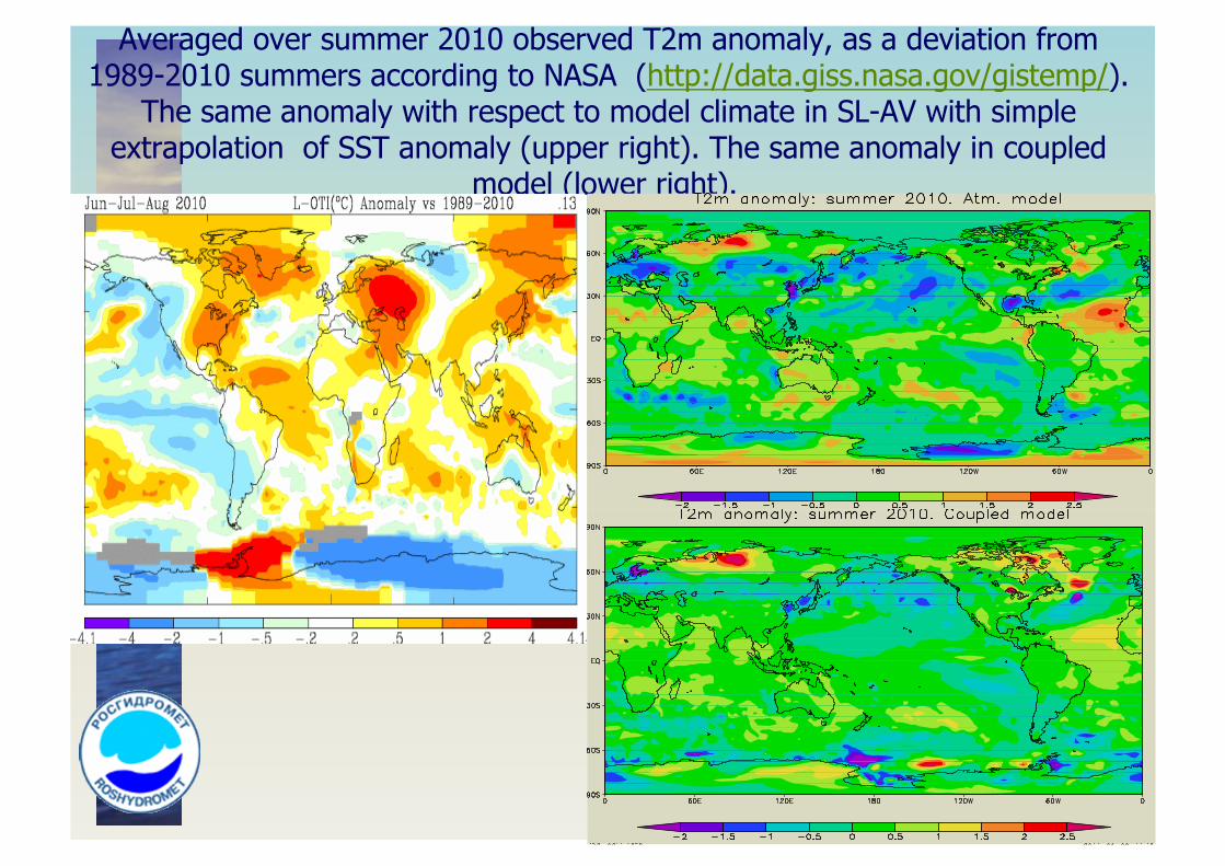
Averaged over summer 2010 observed T2m anomaly, as a deviation from 1989-2010 summers according to NASA (http://data.giss.nasa.gov/gistemp/).

The same anomaly with respect to model climate in SL-AV with simple extrapolation of SST anomaly (upper right). The same anomaly in coupled

model (lower right).

Further work on coupled model for seasonal forecasts

  Trying to refine initial condition in soil (own assimilation of 2m variables).

  Trying CLIRAD SW radiation parameterization.   Likely switching to ERA-Interim reanalyses for

hindcasts.   Numerical experiments using ocean data

assimilation system developed in Hydrometcentre of Russia.

  Using higher resolution ocean model, more sophisticated ice model.

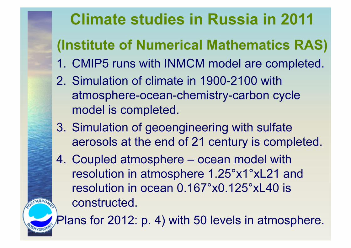
Climate studies in Russia in 2011 (Institute of Numerical Mathematics RAS) 1.  CMIP5 runs with INMCM model are completed. 2.  Simulation of climate in 1900-2100 with

atmosphere-ocean-chemistry-carbon cycle model is completed.

3.  Simulation of geoengineering with sulfate aerosols at the end of 21 century is completed.

4.  Coupled atmosphere – ocean model with resolution in atmosphere 1.25°x1°xL21 and resolution in ocean 0.167°x0.125°xL40 is constructed.

Plans for 2012: p. 4) with 50 levels in atmosphere.

Global temperature (top) and CO2 (bottom) in 2070-2100 without (red) and with (blue)

geoengineering

Thank you for attention!