A unified Bang-bang principle June 08 2010 - Fields Institute · A unified "Bang-Bang" Principle...
47
A unified "Bang-Bang" Principle with respect to a class of non-anticipative benchmarks Phillip Yam (Joint work with Prof. S. P. Yung (Math, HKU), W. Zhou (Math, HKU), John Wright (Math, HKU), Prof. Eddie Hui (BRE, HKPU))
Transcript of A unified Bang-bang principle June 08 2010 - Fields Institute · A unified "Bang-Bang" Principle...

A unified "Bang-Bang" Principle with respect
to a class of non-anticipative benchmarks
Phillip Yam
(Joint work with Prof. S. P. Yung (Math, HKU), W. Zhou (Math, HKU), John Wright (Math, HKU),
Prof. Eddie Hui (BRE, HKPU))

Outline:
� What is the right time to sell a stock?
� A unified “Bang-Bang” (algebraic) principle
� How long is a financial crisis? Sell-in-May?
Halloween effect?

What is the right time to sell a stock?
(Supported by HKRGC: HKGRF 502909)
(Joint work with Prof. S. P. Yung and W. Zhou (Math, HKU))

A voice from an individual investor:
down-to-earth concern
� In a finite time horizon [0, T],
(1) Selling it at the highest price,
(2) Buying a stock at the lowest price
with NO RISK.
� Mission impossible! At any time, nobody can anticipate the future,
� Better ask:
(1) How can we minimize the “gap” between the selling (resp. buying) price of a stock and its ultimate maximum (resp. minimum)?
Or (2) How can maximize the chance to sell (resp. buy) a stock precisely at its ultimate maximum (resp. ultimate minimum)?
Or (3) Avoiding selling stock at least price, i.e. maximizing the gap between selling price (resp. buying) and the ultimate minimum price (resp. maximum), … … etc.
� Can “technical analysis” help?
For example, looking at chart to seek for patterns, trends, waves, etc.

An inquiry from Mathematics
Community – A. N. Shiryaev (1999)
� St follows a geometric Brownian motion
dSt = St ( µ dt + σ dBt )
� Measuring the “gap” by using:
(1) Mean Square Difference, see Peskir and Shiryaev (2001) & (2006) and Du Toit and Peskir (2007); for partial results with p(>1)-power, see Gaversen, Shiryaev and Peskir (2001), Pedersen (2003), Du Toit and Peskir (2007)
(2) Mean Relative Error of the selling price to the highest price ST* over [0, T]:
Relative error = (ST* – St) / ST
*
i.e. define:
(i) PDE method: Shiryaev, Xu and Zhou (2009)
(ii) Probabilistic method: Du Toit and Peskir (2009), Yam, Yung and Zhou (2009).

Optimal selling time
� For any stopping time, we define
� The optimal stopping times for different cases are:
� where

A stock with (µ, σ ) is called:
1) Superior if µ / σ2 > ½
2) Neutral if µ / σ2 = ½
3) Inferior if µ / σ2 < ½
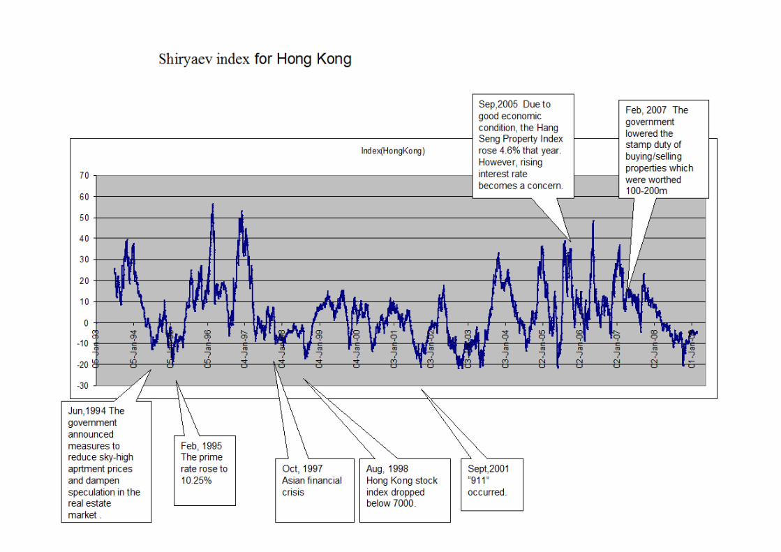
In honor of the problem-poser, we call
µ / σ2 – Shiryaev index of the stock.
Superior, neutral and inferior
stocks
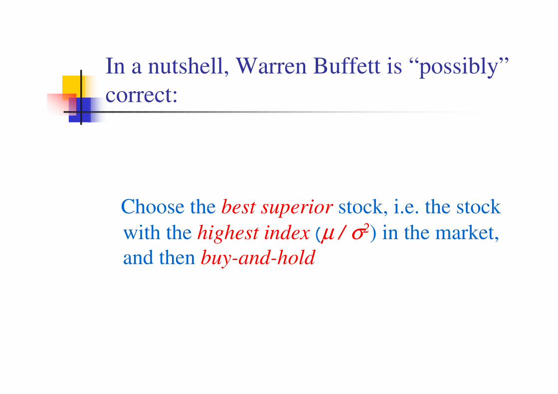
In a nutshell, Warren Buffett is “possibly”
correct:
Choose the best superior stock, i.e. the stock
with the highest index (µ / σ2) in the market,
and then buy-and-hold

Idea of Proof

A Princess looking for her Prince
Charming (Secretary Problem)
� For if a princess can expect to meet exactly N
eligible gentlemen in her life, what strategy should
she use to maximize her chance of choosing the
best one?
� An optimal strategy for selecting the best of these
N candidates in row is to ‘skip’ the first j*-1
candidates, and then select the next "best so far"
that she would encounter.
� Here j* =4 for N = 10, say.

Inspired by the Princess
� For any stopping time, we define
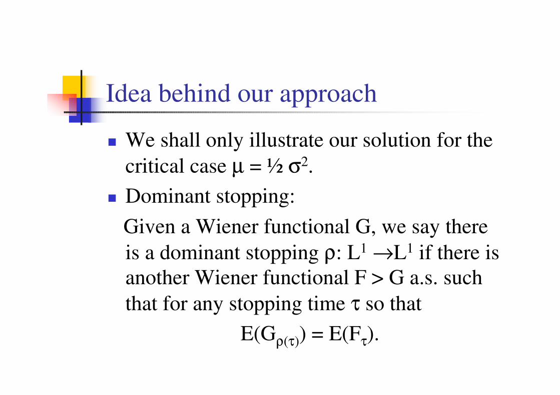
Idea behind our approach
� We shall only illustrate our solution for the
critical case µ = ½ σ2.
� Dominant stopping:
Given a Wiener functional G, we say there
is a dominant stopping ρ: L1 →L1 if there is
another Wiener functional F > G a.s. such
that for any stopping time τ so that
E(Gρ(τ)) = E(Fτ).

� We first use Strong Markov Property to
simplify:
� where is the reflected
Brownian motion at zero and
Sketch of the proof for µ / σ2 = ½

� Similarly, we also have
� where

F > G
� They agree along the boundaries x = 0 and t
= 0.
� Both F and G approach zero as either x and
t gets large.
� Show by contradiction that there is no
interior global minimum with negative
value.

�
where
Good notations can ease the
argument
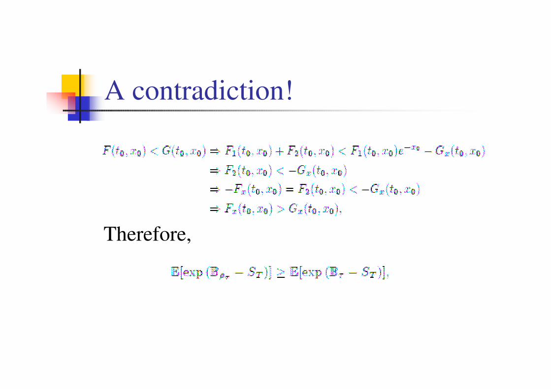
A contradiction!
Therefore,

is actually constant!
� Let
� Using Ito-Tanaka’s formula:
� Fx(t, 0) = 0 and together with Optional Stopping
Theorem, we have

� Hence we have
� It is optimal to sell the stock when the
underlying governing Brownian motion hits
its running maximum or at the terminal time.

A unified “Bang-Bang” principle

Generalizations � General processes (Probabilistic methods):
(i) Binomial tree (CRR) processes (Yam, Yung and Zhou (2009));
(ii) Levy processes (Allaart (2009a, b)).
� General benchmarks:
(i) Maximizing the probability to sell a stock at ultimate maximum (Yam, Yung and Zhou (2009));
(ii) (behavioral sense) non-increasing and convex function f:
Dai, Jin, Zhong and Zhou (2009) (PDE methods);
(iii) (Conservative mind) Selling as far as possible from the lowest price
Dai, Jin, Zhong and Zhou (2009) (PDE methods);
(iv) Selling as close as “average” price (See Dai and Zhong (2009) (PDE methods))
where
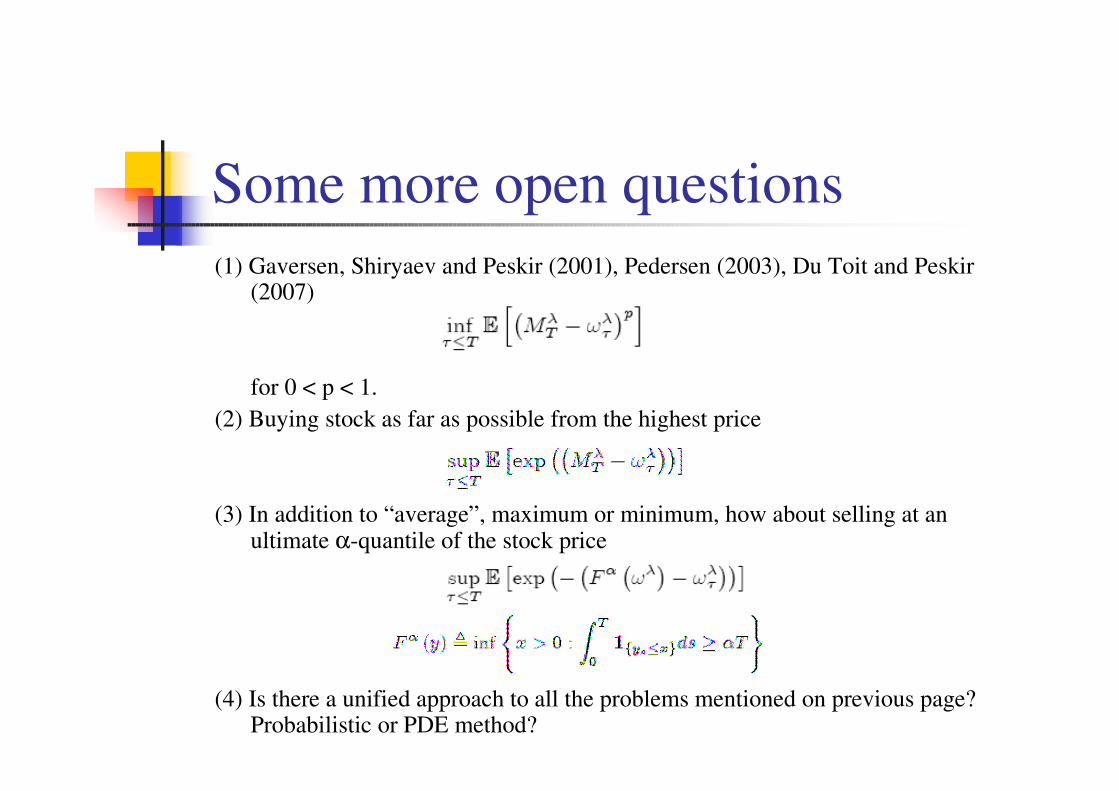
Some more open questions
(1) Gaversen, Shiryaev and Peskir (2001), Pedersen (2003), Du Toit and Peskir(2007)
for 0 < p < 1.
(2) Buying stock as far as possible from the highest price
(3) In addition to “average”, maximum or minimum, how about selling at an ultimate α-quantile of the stock price
(4) Is there a unified approach to all the problems mentioned on previous page? Probabilistic or PDE method?

A unified (algebraic) principle
� Yes, a probabilistic approach! One result for all!
� D[0,T] = space of all piecewise continuous paths
with at most finitely many “ordinary” jump points
� Using “Permutation” and/or “time reversing” of
different “pieces” of a path in D[0,T] to define an
equivalent relation R in D[0,T]
~

A universal benchmark F
Consider a Wiener functional F such that:
1. Translation invariant:
F(w + c) = F(w) + c ;
2. Monotonicity:
For every t, w1(t) ≥ w2(t), implies F(w1) ≥ F(w2);
3. F is R-invariant.
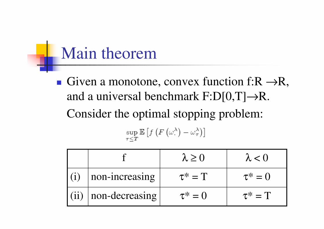
Main theorem
� Given a monotone, convex function f:R →R,
and a universal benchmark F:D[0,T]→R.
Consider the optimal stopping problem:
τ* = Tτ* = 0non-decreasing(ii)
τ* = 0τ* = Tnon-increasing(i)
λ < 0λ ≥ 0f

Idea of proof
1. Comparison of stopping times is equivalent to comparison of magnitude of functions;
2. Application of time reversibility of Brownian motion (or in general infinitely divisible processes) leads convexity of f to come to play; indeed, the difference of functions in (1) can now be expressed as an integral of difference of increments of f over consecutive disjoint intervals;
3. Simple convexity analysis deduces the non-negativity of the difference of functions in (1).
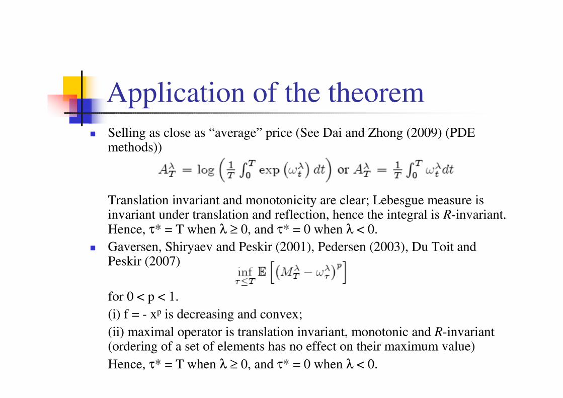
Application of the theorem
� Selling as close as “average” price (See Dai and Zhong (2009) (PDE methods))
Translation invariant and monotonicity are clear; Lebesgue measure is invariant under translation and reflection, hence the integral is R-invariant. Hence, τ* = T when λ ≥ 0, and τ* = 0 when λ < 0.
� Gaversen, Shiryaev and Peskir (2001), Pedersen (2003), Du Toit andPeskir (2007)
for 0 < p < 1.
(i) f = - xp is decreasing and convex;
(ii) maximal operator is translation invariant, monotonic and R-invariant (ordering of a set of elements has no effect on their maximum value)
Hence, τ* = T when λ ≥ 0, and τ* = 0 when λ < 0.
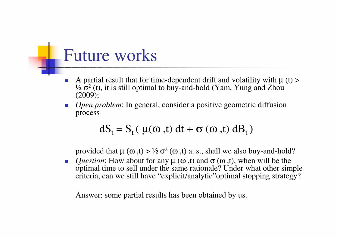
Future works
� A partial result that for time-dependent drift and volatility with µ (t) > ½ σ2 (t), it is still optimal to buy-and-hold (Yam, Yung and Zhou(2009);
� Open problem: In general, consider a positive geometric diffusion process
provided that µ (ω ,t) > ½ σ2 (ω ,t) a. s., shall we also buy-and-hold?
� Question: How about for any µ (ω ,t) and σ (ω ,t), when will be the optimal time to sell under the same rationale? Under what other simple criteria, can we still have “explicit/analytic”optimal stopping strategy?
Answer: some partial results has been obtained by us.
dSt = St ( µ(ω ,t) dt + σ (ω ,t) dBt )

How long will a financial crisis be?
Sell-in-May and Go-Away?
Welcome Halloween?
(Supported by HKPU Interdisciplinary Grant, and HKPU IRG A-PC0D)
(Joint work with John Wright (Math, HKU) and Prof. Eddie C. M. Hui (BRE, HKPU))
Implication of Shiryaev index on
Seasonal Effects in Markets

Sell-In-May, Welcome Halloween? (http://en.wikipedia.org/wiki/Sell_in_May)
� “ … ‘Sell in May and go away’, the belief that the period from November to April inclusive has significantly stronger growth on average than the other months …”
� “ … stocks are sold at the start of May and the proceeds held in bonds or a deposit account; stocks are bought again in the autumn, typically around Halloween.”
� “ … ‘Halloween indicator’ is more prevalent in Europe than in the United States, …”
� “ … There is no consensus on what causes this phenomenon, although theories include an impact from summer vacations and draw comparisons to the January effect. …”
Preliminaries on modeling
� Any continuous semimartingale is a sum of finite variation process and a Brownian motion up to change of time (continuous local martinagale);
� It is reasonable to model positive stock price dynamics as a general geometric diffusion process with adapted stochastic drift and volatility
� From experience, stock price time series seems to have long-memory (or long-range) dependence. Why not use fractional Brownian motion as a model?
1) Most statistical tests are only testing the autocorrelation structure of a time series, no immediate test can differentiate whether the underlying process is a fBM or a Gaussian process with the same autocorrelation structure (see L. C. G. Rogers (1997));
2) Apart from a few results, e.g. no-arbitrage nature of market driven by fBMwith appropriate proportional transaction cost (and the corresponding fundamental theorem of asset pricing but no pricing formula is provided), there is no convenient stochastic calculus for non-semimartingales (perhaps rough path theory, see T. Lyons (1998)).

Model in Practice (Moving Average)
� Source of data: 20+ years of Hang-Seng index;
� We assume that the Hang-Seng index St follows a geometric Brownian motion over a moving window (reasonably to take 4 to 6 months):
Or
� Treating drift and volatility as if constant over the moving window;
� Using AR(1) model to fit the data over the moving window, and hence the estimation of parameters. No significant statistical rejection had observed;
� Using Graduation (smoothing) method to produce secondary estimates of parameters.
� Perhaps More sophisticated modeling, e.g. GARCH and their generalized versions, may provide similar figures.
tt
t
dSdt dB
Sµ σ= +
2
0
1
2( ) ( ) ( )
t tlog S log S t Bσµ σ= + − +

Graphs of log(St-St-1) 1989-1992
1989 T Line Fit Plot
-0.4
-0.3
-0.2
-0.1
0
0.1
0.2
0 100 200 300
T
u_i
1990 T Line Fit Plot
-0.08
-0.06
-0.04
-0.02
0
0.02
0.04
0.06
0.08
0 50 100 150 200 250 300
T
u_i
1991 T Line Fit Plot
-0.08
-0.06
-0.04
-0.02
0
0.02
0.04
0.06
0 50 100 150 200 250 300
T
u_i
1992 T Line Fit Plot
-0.06
-0.04
-0.02
0
0.02
0.04
0.06
0 100 200 300
T
u_
i

Graphs of log(St-St-1) 1993-1996
1993 T Line Fit Plot
-0.1
-0.05
0
0.05
0.1
0 100 200 300
T
u_
i
1994 T Line Fit Plot
-0.1
-0.05
0
0.05
0.1
0 50 100 150 200 250 300
T
u_i
1995 T Line Fit Plot
-0.06
-0.04
-0.02
0
0.02
0.04
0.06
0.08
0 50 100 150 200 250 300
T
u_
i
1996 T Line Fit Plot
-0.1
-0.05
0
0.05
0 50 100 150 200 250 300
T
u_
i
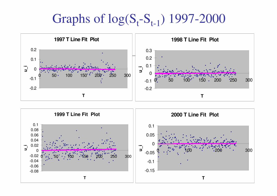
Graphs of log(St-St-1) 1997-2000
1997 T Line Fit Plot
-0.2
-0.1
0
0.1
0.2
0 50 100 150 200 250 300
T
u_
i
1998 T Line Fit Plot
-0.2
-0.1
0
0.1
0.2
0.3
0 50 100 150 200 250 300
T
u_i
1999 T Line Fit Plot
-0.08
-0.06
-0.04
-0.02
0
0.02
0.04
0.06
0.08
0.1
0 50 100 150 200 250 300
T
u_i
2000 T Line Fit Plot
-0.15
-0.1
-0.05
0
0.05
0.1
0 100 200 300
T
u_i

Graphs of log(St-St-1) 2001-2004
2001 T Line Fit Plot
-0.15
-0.1
-0.05
0
0.05
0.1
0 50 100 150 200 250 300
T
u_i
2002 T Line Fit Plot
-0.06
-0.04
-0.02
0
0.02
0.04
0.06
0.08
0 100 200 300
T
u_
i
2003 T Line Fit Plot
-0.06
-0.04
-0.02
0
0.02
0.04
0.06
0.08
0 100 200 300
T
u_i
2004 T Line Fit Plot
-0.08
-0.06
-0.04
-0.02
0
0.02
0.04
0.06
0.08
0 50 100 150 200 250 300
T
u_
i

Graphs of log(St-St-1) 2005-2008
2005 T Line Fit Plot
-0.06
-0.04
-0.02
0
0.02
0.04
0 50 100 150 200 250 300
T
u_
i
2006 T Line Fit Plot
-0.06
-0.04
-0.02
0
0.02
0.04
0.06
0 50 100 150 200 250 300
T
u_i
2007 T Line Fit Plot
-0.1
-0.05
0
0.05
0.1
0 50 100 150 200 250 300
T
u_
i
2008 T Line Fit Plot
-0.1
-0.05
0
0.05
0.1
0.15
0 50 100 150 200
T
u_i

Projecting the duration of a
financial crisis based on
Shiryaev index
(Moving window before each time point)

Seasonal Effects and Shiryaev index:
Sell-in-May?
And
Halloween Effect?
(Each time point is the mid-point of the moving window)

United Kingdom market
Monthly Comparison
73.2
1%
63.6
4%
59.8
0%
57.7
8%
53.5
5%
48.5
2%
46.0
8%
50.3
6%
49.2
6%
50.7
1%58
.97%
64.0
5%
26.7
9%
36.3
6%
40.2
0%
42.2
2%
46.4
5%
51.4
8%
53.9
2%
49.6
4%
50.7
4%
49.2
9%
41.0
3%
35.9
5%
0%
20%
40%
60%
80%
100%
1 2 3 4 5 6 7 8 9 10 11 12
Month
positive negative

United States market
Monthly Comparison
51.3
8%61
.60%
65.3
8%
62.7
2%
65.4
0%
53.0
7%
50.5
2%
37.2
8%
29.1
4%
32.6
8%
35.6
2%
41.6
1%
48.6
2%
38.4
0%
34.6
2%
37.2
8%
34.6
0%
46.9
3%
49.4
8%
62.7
2%
70.8
6%
67.3
2%
64.3
8%
58.3
9%
0%
20%
40%
60%
80%
100%
1 2 3 4 5 6 7 8 9 10 11 12
Month
positive negative

In a given year, western market seems to lull
in summers after May and to get better in
winters.

Hong Kong market
Monthly Comparison
47.4
5%
42.2
4%
40.0
6%51
.33%
52.6
8%
57.4
3%
59.7
7%67
.04%
57.4
3%
63.8
4% 78.8
7%
70.6
9%
52.5
5%
57.7
6%
59.9
4%
48.6
7%
47.3
2%
42.5
7%
40.2
3%
32.9
6%
42.5
7%
36.1
6% 21.1
3%
29.3
1%
0%
20%
40%
60%
80%
100%
1 2 3 4 5 6 7 8 9 10 11 12
Month
Positive Negative

In a given year, market seems to fall silent
after Lunar New Year, yet it seems to get
better after Dragon-Boat festival.
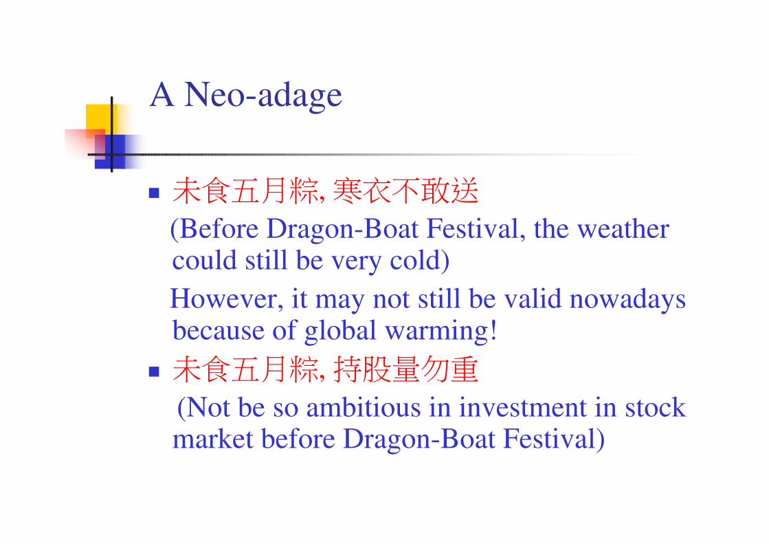
� 未食五月粽, 寒衣不敢送
(Before Dragon-Boat Festival, the weather could still be very cold)
However, it may not still be valid nowadays because of global warming!
� 未食五月粽, 持股量勿重
(Not be so ambitious in investment in stock market before Dragon-Boat Festival)
A Neo-adage

Thank you!