A TRANSIENT COMPUTATIONAL FLUID DYNAMIC STUDY OF A ...
130
A TRANSIENT COMPUTATIONAL FLUID DYNAMIC STUDY OF A LABORATORY-SCALE FLUORINE ELECTROLYSIS CELL by Ryno Pretorius, Supervisor: Prof. P.L. Crouse Student Number: 25028996/04423372 Submitted in fulfilment of the requirements for the degree Masters in Chemical Engineering in the Faculty of Engineering, Built Environment and Information Technology University of Pretoria Date of submission: 2011/07/07 © University of Pretoria
Transcript of A TRANSIENT COMPUTATIONAL FLUID DYNAMIC STUDY OF A ...

A TRANSIENT COMPUTATIONAL FLUID DYNAMIC
STUDY OF A LABORATORY-SCALE FLUORINE
ELECTROLYSIS CELL
by Ryno Pretorius
Supervisor Prof PL Crouse
Student Number 2502899604423372
Submitted in fulfilment of the requirements for the degree Masters in Chemical
Engineering in the Faculty of Engineering Built Environment and Information
Technology University of Pretoria
Date of submission 20110707
copycopy UUnniivveerrssiittyy ooff PPrreettoorriiaa
i
A TRANSIENT COMPUTATIONAL FLUID DYNAMIC
STUDY OF A LABORATORY-SCALE FLUORINE
ELECTROLYSIS CELL
Synopsis
Fluorine gas is produced industrially by electrolysing hydrogen fluoride in a
potassium acid fluoride electrolyte Fluorine is produced at the carbon anode
while hydrogen is produced at the mild-steel cathode The fluorine produced has
a wide range of uses most notably in the nuclear industry where it is used to
separate 235U and 238U The South African Nuclear Energy Corporation (Necsa)
is a producer of fluorine and requested an investigation into the hydrodynamics
of their electrolysis cells as part of a larger national initiative to beneficiate more
of South Africarsquos large fluorspar deposits
Due to the extremely corrosive and toxic environment inside a typical fluorine
electrolysis reactor the fluid dynamics in the reactor are not understood well
enough The harsh conditions make detailed experimental investigation of the
reactors extremely dangerous The objective of this project is to construct a
model that can accurately predict the physical processes involved in the
production of fluorine gas The results of the simulation will be compared to
experimental results from tests done on a lab-scale reactor A good correlation
between reality and the simulacrum would mean engineers and designers can
interrogate the inner operation of said reactors safely effortlessly and
economically
This contribution reports a time-dependent simulation of a fluorine-producing
electrolysis reactor COMSOL Multiphysics was used as a tool to construct a two
dimensional model where the charge- heat- mass- and momentum transfer
were fully coupled in one transient simulation COMSOL is a finite element
ii
analysis software package It enables the user to specify the dimensions of
hisher investigation and specify a set of partial differential equations boundary
conditions and starting values These equations can be coupled to ensure that
the complex interaction between the various physical phenomena can be taken
into account - an absolute necessity in a model as complex as this one
Results produced include a set of time dependent graphics where the charge-
heat- mass- and momentum transfer inside the reactor and their development
can be visualized clearly The average liquid velocity in the reactor was also
simulated and it was found that this value stabilises after around 90 s The
results of each transfer module are also shown at 100 s where it is assumed that
the simulation has achieved a quasi-steady state
The reactor on which the model is based is currently under construction and will
be operated under the same conditions as specified in the model The reactor
constructed of stainless steel has a transparent side window through which both
electrodes can clearly be seen Thus the bubble formation and flow in the reactor
can be studied effectively Temperature will be measured with a set of
thermocouples imbedded in PTFE throughout the reactor The electric field will
similarly be measured using electric induction probes
KEYWORDS Fluid dynamics fluorine electrolysis coupled analysis COMSOL
Multiphysics hydrodynamics
iii
Contents
1 Introduction 1
2 Literature 4
21 Introduction 4
211 Gas Evolution 4
212 Metal Deposition 6
213 Other Electrolysis reactors 8
22 Historical 10
23 Industrial Manufacture of Fluorine 14
24 Description of a Fluorine Electrolysis Reactor 14
241 Basic Operations 14
242 Electrolyte 15
2421 Electrolyte Properties 15
2422 Electrolyte Manufacture and Specifications 20
243 Anode and Anode Phenomena 21
2431 Polarisation 22
2432 Overvoltage 23
244 Cathode Cell-Body and Skirting 25
245 Reversible and Working Voltage 25
246 Heat Production and Energy Efficiency 26
247 Fundamental Equations for Transport in Diluted Solutions 27
248 Product Gasses 30
2481 Hydrogen and Fluorine 30
2482 Hydrogen Fluoride 31
25 Published Fluorine Cell Simulations 32
251 Modelling coupled transfers in an industrial fluorine electrolyser
(Roustan et al 1997) 32
252 Modeling of the Trajectories of the Hydrogen Bubbles in a Fluorine
Production Cell (Hur et al 2003) 38
253 Effect of hydrodynamics on Faradaic current efficiency in a fluorine
electrolyser (Espinasse et al 2006) 42
iv
254 Electrochemical Engineering Modelling of the Electrodes Kinetic
Properties during Two-Phase Sustainable Electrolysis (Mandin et al 2009)
45
255 Modeling and Simulation of Dispersed Two-Phase Flow Transport
Phenomena in Electrochemical Processes General Conclusion (Nierhaus et
al 2009) 46
26 In summary 48
3 Model Development 51
31 Reactor Description 51
32 Model Description 51
321 Momentum Transfer 53
322 Heat Transfer 55
323 Charge Transfer 56
324 Mass Transfer 56
3241 Electrode Reactions 57
325 Starting Conditions 58
326 Boundary Conditions 58
327 Constants 63
328 Expressions 64
329 Mathematical Solution 65
3291 Solution Method 67
3292 Meshing 68
3293 Computing 73
4 Results and Discussion 75
41 Momentum Transfer 76
411 Time Progression 81
42 Heat Transfer 85
421 Time Progression 87
422 Parametric Study 89
43 Charge Transfer 92
44 Mass Transfer 98
v
441 Time Progression 100
45 Simulations of Published Results 103
451 Modelling coupled transfers in an industrial fluorine electrolyser
(Roustan et al 1997) 103
452 Effect of hydrodynamics on Faradaic current efficiency in a fluorine
electrolyser (Espinasse et al 2006) 108
5 Conclusions and Recommendations 112
51 Experimental Design Simulation 112
511 Momentum Transfer 112
512 Heat Transfer 113
513 Charge Transfer 114
514 Mass Transfer 114
52 Comparison with Published Results 115
521 Effect of hydrodynamics on Faradaic current efficiency in a fluorine
electrolyser (Espinasse et al 2006) 115
522 Modelling coupled transfers in an industrial fluorine electrolyser
(Roustan et al 1997) 115
6 Acknowledgments 116
7 References 116
vi
Nomenclature
List of Symbols
VariableConstant Description Units
iC Concentration of chemical species i 3mmol
iC 0 Initial concentration of species i 3mmol
pC Heat capacity at constant pressure 11 KkgJ
0pC Heat capacity at constant pressure at 25 degC 11 KkgJ
bd Average bubble diameter m
ied Inter-electrode distance m
iD Isotropic diffusion coefficient for chemical
species i
12 sm
E Electric field 1mV
F
Volume force vector 222 mskg
F Faradays constant 1 molsA
g
Gravitational acceleration 2 sm
i Current density at specific point in reactor 2mA
ni Current density for electrode n 2mA
0i Exchange current density 2mA
I
Current A
ik Electrode rate constants 1 sm
itk Thermal conductivity of material i 11 KmW
iN
Molar flux of species i in the electrolyte 12 smmol
n Stoichiometric factor coefficient (-)
n Normal vector (-)
P Pressure kPa
ip Reaction order for anodic species (-)
rtrP _ Pressure of atmosphere inside reactor kPa
vii
Q Internal heat source 3mW
q Internal heat source W
iq Reaction order for cathodic species (-)
gR Ideal gas constant 11 KmolJ
iR Molar flux of species i frominto the electrode
surface
12 smmol
ir Reaction rate of specie i in the electrolyte 13 smmol
is Stoichiometric coefficient of species i in
electrode reaction
(-)
T Temperature of electrolyte K
t Time s
0T Initial electrolyte temperature K
wT Wall temperature in contact with heating
jacket
K
u Velocity vector 1 sm
iz Charge number of ionic species i (-)
List of Greek Symbols
VariableConstant Description Units
i Electron transfer coefficient (-)
Thermal expansion coefficient of
electrolyte
1C
r Relative permittivity (-)
Cell current efficiency (-)
Cell electric potential V
i0 Reference potential of electrode i V
RV Reversible cell voltage V
TN Thermoneutral cell voltage V
viii
i Volume fraction of phase i (-)
i Viscosity of fluid phase i sPa
s Surface overpotential V
i Electrical conductivity of material i 1mS
im Ionic mobility of species i 112 sJmolm
Electrolyte density 3mkg
g Ideal gas molar density 1molkg
0 Electrolyte density at 25 degC 3mkg
1
1 Introduction
Fluorine gas is produced industrially via electrolysis of hydrogen fluoride HF
Two gasses are liberated viz hydrogen 2H and fluorine 2F Fluorine the more
valuable product has a wide range of uses Initially limited to the nuclear
industry other uses were found as fluorine became more readily available
The Nuclear Energy Corporation of South Africa (NECSA) wishes to better
understand the mechanism of gas evolution inside their fluorine electrolysis
reactors To date these reactors have been controlled using a black-box
approach due to the hostile environment inside the reactors which makes it very
difficult and also dangerous to investigate the inner workings of the reactor
adequately A detailed simulation will provide the engineering team with a better
understanding of these inner workings in order to optimise fluorine production
The objective of this investigation is to construct a model that can accurately
predict the physical processes involved in the production of fluorine gas The
specifications of a lab-scale fluorine cell were used for these simulations This
cell is currently under construction Once completed the results of the simulation
will be compared to the experimental data gathered
A second set of simulations of fluorine cell data published in the open literature
were conducted The good correlation between the results achieved in this work
and those in the literature serve as strong support of the accuracy of the
modelling procedure followed If satisfactory comparative results are obtained
modelling of the industrial scale reactor can commence This knowledge will give
design engineers a clearer idea of how to design and more efficiently operate
fluorine electrolysis reactors
Modelling was done on the software package COMSOL Multiphysics which
employs the Finite Element Method (FEM) to solve systems of partial differential
2
equations Only the electrolyte phase is modelled incorporating the fundamental
equations describing electric field mass- heat- and momentum transport The
effects of the gaseous phase are included by modifying select liquid phase
equations to include the effects of a gaseous phase
Chapter two of this dissertation gives a review of electrolysis in general industrial
electrolysers and looks at fluorine electrolysis in more detail The history of
fluorine is investigated its uses and production up to the industrial standard
widely used today The modern fluorine electrolysis reactor is then described in
terms of all its components products and reactants This includes sections on
electrolyte properties and manufacture anode and anode phenomena cathode
cell body and skirting characteristics fundamental transport equations and
product gas descriptions This review takes a closer look at available published
fluorine cell simulations Data from this section are used for comparison with
COMSOL simulations
The third chapter describes the simulation where the behaviour of the potassium
acid fluoride HFKF 2 electrolyte is modelled The stirring effects of the
gaseous products due to convection are included in the simulations This is done
by using a modified Navier-Stokes equation that takes into account the gas
phase by adjusting the equation with a volume fraction factor at each relevant
term All relevant equations for mass- heat- charge- and momentum transfer
used during simulation are shown as well as the physical parameters used The
chapter is concluded with a section on the mathematical and FEM characteristics
of the modelling process The physical characteristics of the product gasses and
the effects they have on the electrodes are beyond the scope of this
investigation
Results discussed in this investigation include graphical representations of the
momentum- heat- charge- and mass transfer simulations Time progression in
the reactor is shown in each case where meaningful results were obtained A
3
parametric study of the effect of varying the thermal conductivity of the electrolyte
is also included A detailed comparison is drawn between the COMSOL
simulations and the published simulations
Finally summary conclusions are drawn from the results and a series of
recommendations is made
4
2 Literature
21 Introduction
Electrolysis is a branch of electrochemistry where a direct current is applied to
drive an otherwise none-spontaneous reaction It has high commercial
importance where it is used to separate elements from ores and solutions via an
electrolyte The process requires a direct current to pass through an ionic
substance (electrolyte) between two electrodes the anode and cathode (Walsh
1993 13)
Metal semi-conductor conductive ceramics or polymers and graphite electrodes
are commonly used Carbon electrodes less commonly so but are necessary in
special electrolysers used during fluorine production Ions and atoms are
interchanged and electrons are removed or added via the external circuit
Charged ions are attracted to opposite electrodes The products are collected
and taken for further processing Gasses are collected and purified whereas
metals collect on the electrode surfaces Energy required is the sum of change in
Gibbs free energy plus other energy losses incurred in the system The electric
input commonly exceeds the required to facilitate the reaction this energy is
released in the form of heat (Walsh 1993 13)
Common industrial electrode processes include gas evolution metal deposition
metal dissolution transformation of existing surface phases oxidation of a fuel
change in oxidation state of a solute metal ion and the hydrodimerisation of an
activated olefin (Walsh 1993 17)
211 Gas Evolution
Chlorine
Chlorine was first produced electrochemically by Cruikshank in 1800 but was not
economically viable In 1892 advances in power generator and anode production
5
techniques made the production of chlorine gas from the chlor-alkali possible on
an industrial scale This process still produces most of the worlds chlorine gas
supply (Schmittinger 2003)
The chlor-alkali process intails passing a direct current through an aqueous
solution of sodium chloride This will in turn decompose the electrolyte to produce
chlorine hydrogen and sodium hydroxide solution The three different processes
used to produce chlorine are the diaphragm cell process the mercury cell
process and the more recently developed membrane cell process Each method
represents a different method of keeping the chlorine produced at the anode
separate from the caustic soda and hydrogen produced at the cathode Chlorine
is also produced as a byproduct is the electrolysis of hydrochloric acid and
molten alkali and alkaline earth metal chlorides Chlorine production is the worlds
largest consumer of industrial electricity and therefore the most significant
gaseous product produced by electrolysis (Schmittinger 2003)
Fluorine
Fluorine gas is produced from the electrolysis of hydrogen fluoride in an
electrolyte and will be discussed at length in chapters to follow
Hydrogen
Hydrogen the most basic element is mainly produced from hydrocarbons on an
industrial scale but can also be produced form by electrolysis or as a byproduct
of electrolytic processes Electrolytically produced hydrogen only accounts for
5 of global supply An aqueous solution of ionic salts (used to increase the
conductivity of water) is used as electrolyte and produces hydrogen at the
cathode and oxygen at the anode The cathode and cell body is constructed of
steel or coated steel The cell body is coated with a corrosion resistant material
and the cathode is coated andor acitivated with various catalysts to reduce
hydrogen overvoltage The anode can be constructed of nickel or nickel coated
steel (Haumlussinger et al 2003) Electrolytic hydrogen is very pure but can contain
6
unwanted traces of oxygen which can be removed by reaction with hydrogen
over a platinum catalyst (Schmittinger 2003)
Oxygen
Oxygen is produced industrially by various techniques the most common
technique being fractional distillation of air it can also be produced as a side
product during the electrolysis of water The latter is also used to produce oxygen
for space and underwater craft (Haumlussinger et al 2003)
212 Metal Deposition
This technique is used to produced amongst others the following metals
aluminium lithium potassium sodium magnesium and calcium Some metals
cannot be produced by the electrolysis of the metallic salt in a water solution
dude to the reactivity of said metallic ion with water protons This in turn leads to
the production of hydrogen gas instead of the metal during electrolysis The
metallic salt is used instead as this is water free medium
Aluminium
Industrially aluminium is produced with the Hall-Heacuteroult from alumina ore
dissolved in cryolite AlF3 is added to the molten mixture to reduce the melting
point of cryolite lower surface tension viscosity and density as well as
decreasing the solubility of reduced species Calcium and lithium fluoride can be
added to further lower the operating temperature of this electrolysis cell The
mixture is electrolysed and results in liquid aluminium precipitation at the
cathode this precipitate then sinks to the bottom of the reactor due to the density
difference of the metal and the electrolyte The aluminium removed via a
vacuum operated syphon is then transferred to be cast into ingots The carbon
anode in turn oxidises as it reacts with oxygen produced at this electrode Other
gases produced include CO2 as the carbon anode is consumed and HF from
the AlF3 (Frank et al 2003)
7
Copper
Electrolysis is used to further refine copper that is intended for use in the
electrical industry Impure copper anodes are dissolved electrolytically in acidic
copper sulphate solutions The copper is then deposited onto stainless steel
cathodes The plated copper is then removed from the stainless steel plates and
sent for further processing Impurities are then collected as sludge from the
bottom of the electrolysers (Seidel 2004 a)
Lithium
Lithium is found in nature in mineral deposits and brine solutions The salt is
usually carbonated and chlorinated before the lithium is extracted Most
commonly it is produced from the electrolysis of the molten salt chloride solution
which usually contains potassium chloride as a supporting electrolyte in a Downs
cell Potassium has a higher decomposition potential than that of lithium and will
not interfere with lithium production Cells are fabricated from low 025-03 steel
or carbon steel An alternative method to produce lithium is via electrolysis in
non-protic solvents (Seidel 2004 f)
Magnesium
Three main electrolytic production techniques exist for the production of
magnesium metal al involve the electrolysis of molten magnesium chloride but
differ in the preparation of the electrolyte cell design and by-product treatment
Chloride is produced as by-product and can be recycled or sold Molten
magnesium is sent for processing and is cast as ingots A graphite anode is used
in conjunction with a steel cathode surrounding each anode (Seidel 2004 c)
Potassium
Potassium metal was first produced from the electrolysis of potassium hydroxide
Later electrolysis methods use an electrolyte comprised of KOH K2CO3 and KCl
The Downs process can also be utilised to manufacture potassium metal
8
Electrolytic manufacture of potassium metal has fallen out of favour for the more
commercially viable process of producing potassium from the reaction of the
halide salt with sodium or calcium-carbide to produce potassium and a metallic
halide salt (Burkhardt et al 2003)
Sodium
Commercial production of sodium is done via the electrolysis of molten sodium
chloride in a reactor known as the Downs cell In this process calcium chloride is
added to lower the melting point of the electrolyte as the higher decomposition
potential of calcium will not compromise the purity of the sodium metal The cell
consists of several graphite anodes surrounded by steel cathodes Chlorine is
produced at the one electrode and a mixture of molten calcium and magnesium
metal at the other The mixture is cooled to precipitate calcium metal (Seidel
2004 c)
Zinc
The electrolytic recovery of zinc is favourable in complex ores that do not lend
themselves to pyrometallurgical processes where zinc cannot be concentrated to
significant levels The zinc mineral is oxidised to a crude oxide and leached with
return acids from cells The zinc sulphate solution is purified and electrolysed
(Seidel 2004 e)
213 Other Electrolysis reactors
Electrochemical machining
ElectroChemical Machining (ECM) offers an alternative way of machining hard
surfaces without degrading the tools used to do the machining The process can
be used to smooth surfaces drill holes and form complex shapes (where the
anode takes the shape of the cahode) The metal to be machined (for example
iron) is connected to the positive end of a direct current supply (where the metal
is dissolved) the dissolved metal then precipitates as a metal-hydroxide (in the
9
case of iron) A gas (usually hydrogen) forms at the cathode This method is
used in the following industries aircraft engine industry medical industry car
industry offshore industry manufacturing industry electronics and several hybrid
ECM processes (Seidel 2004 b)
Electroplating
During electroplating or electrodeposition ions of a dissolved metal are plated
onto a metallic or even non-metal electrode (cathode) surface with the advent of
a direct current The dissolved metal is either dissolved from the anode andor
added as a salt The anode metal is dissolved (oxidised) and plated (reduced) at
the cathode The deposited layer imparts the properties (abrasion aesthetic
corrosion and wear resistance) of a more expensive metal to a cheap metal
surface or to build up the metal thickness of undersized parts Commonly coated
metals are cadnium chromium copper gold silver nickel tin and zinc (Seidel
2004 e)
Electrowinning
Electrowinnig can occur from aqueous solutions or fused molten salts In the first
case the metal ore is converted into an acid-soluble form leached with an acid
leached solution is purifiedconcentrated and finally the metal solution is
electrolysed where the metal is deposited on the cathode done during
copperzinc metal purificationproduction The latter case is where the metallic
salt is electrolysed in its molten state as discussed in previous sections where
Aluminium Sodium Lithium and Magnesium metal production is discussed
(Seidel 2004 c)
Organic electrochemistry
Organic electrochemical reactors facilitate an electroorganic reaction where an
organic substance is chemically transformed by an electric current This
technique has been most successfully implemented in the fine chemicals area
10
Pharmaceutical intermediates and high value added chemicals are produced in
medium to small scale production faculties (Seidel 2004 d)
Sodium hydroxide
Sodium hydroxide is most commonly produced from the electrolysis of sodium
chloride in aqueous solution this process produces a sodium hydroxide solution
and forms hydrogen and chlorine gas To create sodium hydroxide crystals the
solution is evaporated until the water content becomes low enough (Minz 2003)
22 Historical
CW Scheele discovered fluorine in 1771 (Groult 2003) Edmond Fremy was the
first to produce small quantities of fluorine gas by the electrolysis of fused
fluorides (Rudge 1971 2) It was however Ferdinand Frederick Henri Moissan
who first produced fluorine in 1886 by the electrolysis of a solution of potassium
hydrogen fluoride in liquid hydrogen fluoride
The electrolysis was done in solution due to the low conductivity of hydrogen
fluoride and iridiumplatinum electrodes were used The reaction chamber was
cooled to -50 degC to lower the partial pressure of hydrogen fluoride Moissan won
a Nobel Prize for this cell which would later be known as a ldquolow temperature cellrdquo
(Groult et al 2007) He died in 1907 shortly after returning from Stockholm The
belief is widely held that he died due to his work with fluorine causing him to
develop acute appendicitis It is however a contentious issue as to how his work
with fluorine could cause appendicitis
Moissanrsquos work with low temperature electrolysis of fluorine was continued by
Otto Ruff using what was essentially a copy of Moissanrsquos cell The high
temperature cell was pioneered in 1919 by Argo and co-workers where molten
anhydrous potassium acid fluoride at 239 degC was used as an electrolyte with a
graphite anode within a cathodic copper container (Rudge 19711-3)
11
The modern medium temperature cell was first used by Lebeau and Damiens in
1925 using a 51 molar percentage of hydrogen fluoride reducing the melting
point to 658 degC This was also the first time a nickel anode was used reducing
polarisation problems previously experienced This work was later refined by
Cady in 1942 where a 41 hydrogen fluoride composition HFKF 2 gave the
system a melting point of 717 degC Cady used a nickel or non-graphitic carbon
anode reducing polarisation problems and solving the disintegration and swelling
problems graphite anodes experience in HFKF 2 Cadys work was the final
nail in the coffin of all other configurations and operating temperatures of fluorine
cells and is now used as standard (Rudge 19711-3)
It was not until the discovery of nuclear fission and all the possibilities it
presented that fluorine production was escalated from purely academic to
industrial scale manufacture Fluorine is used in the preparation of uranium
hexafluoride 6UF made from uranium tetrafluoride 4UF for the diffusional or
centrifugal separation of 235U and 238U (Rudge 19713-5) Uranium tetrafluoride
4UF is manufactured by reacting uranium dioxide with hydrogen fluoride a
precursor used in fluorine gas manufacture (Clark et al 2005) Uranium
hexafluoride is produced by the following equation (Groult 2003)
624 UFFUF
The main consumers of fluorine gas in this early era were the American
ldquoManhattan Projectrdquo and the British ldquoTube Alloyrdquo project for the purposes of
nuclear weapon development Fluorine production at this stage was done with
nickel anodes which didnrsquot present a commercial future due to the high corrosion
rates of the nickel anodes nickel fluoride sludge formation and limited current
efficiency (Rudge 19713-5)
12
Germany also took major strides during the war years for purposes of atomic
energy investigations and principally the incendiary agent chlorine trifluoride The
only German plant of sizable capacity Falkenhagen near Berlin was capable of
producing 600 to 700 tons per year The plant consisted of 60 high temperature
cells with silver cathodes indicating the importance the Germans attached to the
production of fluorine gas during World War II (Rudge 19715-6)
Fluorine is also widely used in the polymer industry Polyolefin and other plastic
containers can be treated with fluorine to make them resistant to permeation and
solution by polar solvents contained within Other polymer surfaces
(polyethylene polypropylene rubber polyester and aramid among others) are
treated with fluorine to improve significantly surface adhesion and dispersion
properties (Shia 2005)
A wide variety of fluorine inorganic compounds are produced and used Sulphur
hexafluoride 6SF a gaseous highly dielectric compound whose electrical- and
thermal stability and ease of handling has made it a sought-after insulating
medium for the production of high voltage electrical switch gear breakers and
substations (Shia 2005)
Sulphur tetrafluoride 4SF is produced under controlled reaction conditions with
sulphur and fluorine It is most commonly used to form fluorochemical
intermediates in the herbicidal and pharmaceutical industries due to its selective
fluorination capability Fluoro-halogen products include chlorine trifluoride used
in 6UF processing and bromine trifluoride used by the oil well industry in
chemical cutting Iodine- and antimony pentafluorides are used as selective
fluorinating agents to produce fluorochemical intermediates Boron trifluoride
3BF can be used as a polymerization initiator a catalyst in some isomerization
alkylation esterification sulfonation reactions and as flux for magnesium
soldering (Shia 2005)
13
Ammonium bifluoride 24HFNH finds uses in the chemical industry as a
fluorinating agent textile industry as neutralizer for alkalides the metal industry
by pickling stainless steel and pre-treatment of metals before phosphating
galvanizing or nickel plating Other uses of ammonium bifluoride include
preservation of wood (Shia 2005)
Lithium hexafluorophosphate 6LiPF is widely used in the notebook computer
mobile phone consumer electronics and electrical vehicle industries where it is
used as electrolyte in lithium-ion batteries (CHENCO GmbH 2007) Other
inorganic fluorochemicals include 3NF (used to plasma etch silicon wafers and in
plasma-enhanced vapour deposition) and 2XeF (used as strong fluorinating
agent and in etching of silicon in the production of micro-electromagnetic
systems) while primary lithium batteries use graphite fluorides electrodes as
cathodes Graphite fluorides are also used as lubricating agents (Groult 2003)
Fluorination of metals like tungsten and rhenium produces the respective volatile
metal hexafluorides ( 6WF and 6ReF ) The vapours produced are employed in the
chemical vapour deposition industry to produce metal coatings and finely formed
components (Shia 2005) Aluminium fluoride 3AlF and cryolite 63 AlFNa are
used in aluminium refinement as a flux they lower the melting temperature and
increase the conductivity of the electrolyte during electrolysis
(CHENCO GmbH 2007)
Fluorinated organic materials are produced using fluorine The first organic
fluorinated materials that come to mind are HydroFluoroCarbons (HFCs) used as
refrigerants (CHENCO GmbH 2007) Other uses include regiospecific
introduction of fluorine into bio-systems for cancer treatment as well as the
manufacture of perfluorinated materials The high thermal and chemical stability
of perfluorocarbons makes them ideal for high temperature lubrication thermal
14
testing of electronic components and speciality fluids for various pumping and
hydraulic applications The high solubility of oxygen in perfluorocarbons
(specifically perfluorinated aliphatics and cycloaliphatics) has led to their use as
synthetic blood substitutes (Shia 2005)
23 Industrial Manufacture of Fluorine
Three basic steps are required to manufacture elemental fluorine namely (Klose
2004 56)
Conversion of fluorspar into anhydrous hydrogen fluoride according to
Equation 2-1
HFCaSOSOHCaF 24422 2-1
Electrolysis of hydrogen fluoride ( HF ) in molten potassium acid fluoride
HFKF 2 resulting in the formation of fluorine gas according to
Equation 2-2
222 FHHF 2-2
Purification of fluorine gas by a separation process
24 Description of a Fluorine Electrolysis Reactor
241 Basic Operations
Fluorine gas production takes place in an electrolysis cell where a molten
potassium acid fluoride electrolyte ( HFKF 2 408 mass percentage HF ) is
subjected to an electric field (Groult 2003) Fluorine gas is liberated at the anode
and hydrogen gas at the cathode Hydrogen fluoride cannot be used due to its
low electrical conductivity (Shia 2005) Industrial cells typically operate at 6 kA
15
utilizing 30 plate carbon anodes Cooling is required and a high current efficiency
expected However low energy efficiency is common (Groult 2003) 18 is
considered commonplace (Rudge 197145) Bubble formation and motion are
major sources of flow in the electrolysis cell The hydrodynamic properties of the
electrolyte and the efficiency of the electrolysis reaction are strongly coupled to
the flow of bubbles in the reactor This is also true for diluted species transport
and electrical performance This is due to the stirring effect of bubble motion and
the high resistivity of bubbles compared to that of the electrolyte
(Mandin et al 2009)
242 Electrolyte
As mentioned above a fluorine-containing salt (potassium acid fluoride) is used
as an electrolyte due to the low electrical conductivity of pure HF The fluorine
containing salt is heated to just above melting point and held at this temperature
during electrolysis It is critical that the solution stays above its melting point to
ensure fluidity Electrolyte entrained with exiting gas streams can solidify in the
gas outlets this can cause clogging and leads to dangerous explosions caused
by explosive recombination of hydrogen and fluorine gas (Shia 2005)
2421 Electrolyte Properties
Modern fluorine electrolysis cells use HFKF 2 as the electrolyte salt The
reason HFKF 2 is specifically used as the potassium fluoride salt is due to the
melting point of the salt at the given composition (408 HF ) see Figure 2-1
Another consideration is the partial pressure of hydrogen fluoride over the
potassium fluoridehydrogen fluoride system and its variations with composition
and temperature see Figure 2-2 (Rudge 1971 7-9)
The usual working limits are a hydrogen fluoride content of between 38 and
42 with the operating temperature ranging between 80 degC and 110 degC The
16
specific mole fraction of HF in HFKF 2 ensures a low HF partial pressure at a
convenient operating temperature It was found that it is advantageous to operate
cells at low hydrogen fluoride concentrations and at lower temperatures
minimizing loss of hydrogen fluoride in the product streams It is however
required to strike a balance between hydrogen fluoride loss (and by extension
removal later in the process) and an increase in working voltage As the
operating temperature and hydrogen fluoride concentration decrease the
conductivity of the electrolyte decreases requiring a higher voltage to maintain
the same production rate (Rudge 1971 7-9)
Figure 2-1 Melting point versus composition diagram for a potassium fluoridehydrogen
fluoride system (Rudge 1971)
17
Electrolyte density variation with temperature is shown in Figure 2-3 while
electrolyte conductivity over the range 37 to 45 hydrogen fluoride at 80 degC to
100 degC is given by Figure 2-4 (Rudge 1971 10-11)
Another property to consider is the surface tension of the various electrolyte
mixtures This is due to the effects surface tension has on the phenomena
occurring on the carbon anodes Surface tension decreases with an increase in
temperature A reduction in HF concentration increases the electrolyte surface
tension for each 1 increase in HF content a surface tension decrease of
about 25 dynecm is observed It was found that water has only a small effect on
surface tension but a myriad of negative effects on the fluorine production
process (Rudge 1971 10-12)
18
Figure 2-2 Partial pressures of hydrogen fluoride over potassium fluoridehydrogen fluoride
system of varying compositions for various electrolyte temperatures (Rudge 1971)
19
Figure 2-3 Potassium fluoridehydrogen fluoride electrolyte density at various compositions
and varying with temperature (Rudge 1971)
A density variation for the electrolyte as a function of temperature and constant
acid number was derived from Figure 2-3 It was assumed that the gradient of
density variation with temperature remains a constant for any acid number of
potassium acid fluorides The equation was then adjusted for acid number by
specifying the density of the specific potassium acid fluoride mixture at 25 degC
The volume expansivity of the electrolyte was predicted using Equation 2-3
(Smith et al 2005 69) An insignificant isothermal compressibility was assumed
20
CTe25
0
2-3
Figure 2-4 Potassium fluoridehydrogen fluoride electrolyte conductivity with variation in
hydrogen fluoride composition for various temperatures (Rudge 1971)
2422 Electrolyte Manufacture and Specifications
Electrolyte is manufactured by adding liquid hydrogen fluoride to solid potassium
fluoride in a steam jacketed steel vessel with cooling water regulating the
exothermic reaction This is done until sufficient product is produced to cover a
dip-pipe used to introduce liquid hydrogen fluoride The vessel is then heated
21
and agitated while liquid hydrogen fluoride is introduced until the required
composition is reached Excess hydrogen fluoride is removed and moved to an
absorption system Composition is regulated by measuring the liquid height in the
tank and therefore the corresponding density Electrolysis only removes
hydrogen fluoride from the electrolyte HF can easily be replaced during
electrolysis (Rudge 1971 13 and Crouse 2010)
Composition specifications vary from manufacturer to manufacturer Two
important and common specifications are low water and sulphur contents Heavy
metal specification is far more inconsistent Some manufacturers add certain
metals to affect fluorine production efficiency Metals like Al and Mg modify the
carbon fluoride surface film increasing charge transfer by formal traces of metal
fluorides (Rudge 1971 13 and Groult 2003)
243 Anode and Anode Phenomena
Anodes are manufactured from non-graphitized carbon Anodes manufactured
from graphite were found to be unsuitable since exfoliation takes place due to
intercalation of the constituents of the melt between the lamellar graphene layers
(Groult 2003)
Anodes are manufactured from petroleum coke and a pitch blend calcined at low
enough temperatures to prevent graphitisation Carbon is used because it has
low electrical resistivity high strength and resistant to fluorine attack During
electrolysis of potassium bifluoride fluorine gas is produced at the positive
electrode or anode (Shia 2005)
The anode connection is considered to have the most detrimental effect on
anode lifetime During the anode lifetime contact resistance has a tendency to
cause corrosion of the metallic contacts causing the carbon anode to break due
to contact loss The resultant reduced contact area leads to the overheating and
22
burning of the remaining carbon still in contact with the current source which
eventually causes catastrophic failure of the anode (Rudge 1971 44)
2431 Polarisation
Polarisation is defined as the condition under which at a fixed voltage a
decrease occurs in the current flowing through the cell to a value which is
significantly smaller than normal operating currents The decrease can be
sudden or gradual The polarisation problem essentially an anodic problem has
plagued both high and medium temperature carbon anode fluorine cells from the
earliest years The problem first reported by Argo and co-workers in 1919 was
attributed to the ldquonon-wettingrdquo effect of the electrolyte on the graphite It was
found that a carbon anode is initially wettable by the electrolyte but even after a
brief current exposure time the contact angle increases to 150ordm and is no longer
ldquowettedrdquo by the melt It has been contributed to the presence of the intercalation
compound nCF later confirmed with X-ray analysis (Rudge 1971 15-18)
Electro-polishing of the surface at higher voltages leads to enhanced fluorine
evolution by making the surface more easily wettable (Crassous et al 2009)
This large contact angle resulted in the formation of lenticular fluorine bubbles
that tend to stick to the anode surface Bubbles do not detach easily and slip up
the electrode due buoyancy forces coalescence or passing of gas from one
bubble to another (Rudge 1971 15-18) In order to prevent the formation of
graphite-oxides yx OHOC )( the water concentration must be kept very low
(below 20 ppm) These graphite oxides in turn form the graphite fluoride film
during fluorination of the electrolyte (Groult et al 2000)
Suggested methods to overcome film formation are either controlling the
compounds in the electrolyte or by preventing gas bubble accumulation Water
content must be minimised (as previously mentioned) addition of nickel salts
(like nickel fluoride) have been proven effective Preliminary electrolysis of the
electrolyte with a nickel anode reduces water content and introduces nickel into
23
the electrolyte although the beneficial nickel effect is usually transient when
introduced via electrolysis Nickel salt addition is a more permanent solution to
the problem In the case of the latter solution porous electrodes have been
shown to be effective The pores must however not be large enough to be
flooded by the electrolyte (Rudge 197121-25)
2432 Overvoltage
Anode overvoltage accounts for more than 30 of the cellrsquos 9-12 V operating
voltage (Shia 2005) XPS studies have shown that a carbon fluoride film forms
on the surface of the anode and causes this overvoltage the same film
responsible for polarisation in the previous section Electrons may be transferred
easily to the electrolyte through the FC film on the anode during fluorine
evolution but the overall composition of the film makes it more difficult (Groult et
al 2000) It has been established that the carbon fluoride film is composed of
graphite intercalation compounds (GICs) where the FC bonds are ionic andor
semi-ionic and non-conducting graphite fluorides xCF (Groult 2003)
The trace graphite fluorides are presumed to inhibit charge transfer Electric
charge transfer is impeded and contact with the electrolyte is lost due to the low
electrical conductivity of the film and the fact that it is strongly non-wetting A
further consequence of the non-wetting characteristics of fluorinated carbon is
the clinging of lenticular fluorine bubbles to the anode surface reducing its
effective surface area A typical contact angle of the fluorine bubble with the
anode is between 120 and 160 degrees explained by the capability of the low
surface energy fluorinated carbon film to repulse the electrolyte Overvoltage is
caused by a carbon fluoride FC solid layer and a fluidized layer composed of
electro-active species HFKHF 2
that diffuse spontaneously under the
gaseous film adding significant resistance (Groult 2003)
24
Thermodynamically HF decomposition requires a potential of 29 V but an
anode-cathode voltage of 8-10 V is required to maintain a current density of
10-12 2dmA in industrial cells The total voltage is the sum of five contributions
(Groult 2003)
Reversible decomposition voltage (asymp29 V)
Ohmic drop in the electrolyte (asymp3 V)
Ohmic drop in the electrodes (asymp05 V)
Cathode overvoltage (asymp02 V)
Anode overvoltage (asymp25 V)
The high anode overvoltage is attributed to the carbon fluoride layer and the
fluidized layer on the anode this film causes poor wettability of the electrode
which in turn results in a small electro-active area (Groult 2003
Groult et al 2000)
The areas not covered by the bubbles now experience all the charge transfer and
become overheated due to the high current density in this relatively small area
and can result in electrode breakdown possibly by vaporisation This effect shifts
position as the bubbles move up the electrode causing a visible sparking effect
possibly due to incandescence of the fluorine gas or heat of reaction of fluorine
with the anode This effect is sometimes called the ldquoAnode Effectrdquo and serves to
electro-polish the anode by burning off the carbon fluoride layer Excessive
water leads to faster electrode erosion as water facilitates the carbon fluoride
layer production (Rudge 1971 19-20)
The unusually high overpotential experienced in a fluorine electrolyser results in
a strong irreversibility at each electrode leading to significant current losses due
to heat generation This interaction necessitates the coupling of the electrical and
thermal transfer phenomena (Roustan et al 1997)
25
244 Cathode Cell-Body and Skirting
Electrolysis of potassium bifluoride results in hydrogen gas production at the
negative electrode (cathode) The cathode and cell-body are mostly
manufactured from steel or Monel but steel is generally used due to its lower
cost
Skirting is used to separate the hydrogen and fluorine gas compartments and is
usually manufactured from magnesium or Monel (Shia 2005) The skirt can
however also be manufactured from steel if cost is an issue at the cost of reactor
durability The presence of the skirt means that the distance between the anode
and cathode is large This in turn results in a large Ohmic drop
(Roustan et al 1997)
During electrolysis it was found that cathode polarisation appears concurrently
with the development of bipolarity of metal parts interposed between cathode and
anode This phenomenon is especially relevant with regard to the diaphragm
skirt Bipolarisation causes hydrogen to form in the fluorine compartment which
could cause explosions at higher bipolar hydrogen production rates Bipolarity
may also cause erosion of the skirt In practice perforations of the interposed
areas between the electrodes prevent the onset of the bipolarisation effect
(Schumb et al 1947)
245 Reversible and Working Voltage
The reversible cell voltage ( RV ) or thermodynamic decomposition voltage is the
minimum potential required for product formation during electrolysis The
electromotive force (emf) is the reversible cell voltage but of opposite sign The
reversible cell voltage is the difference between the reversible electrode
potentials A typical industrial fluorine electrolyser has a reversible cell voltage of
around 92 V (Rudge 1971 34 Heitz amp Kreysa 198693-101) The working
voltage is the voltage applied in cells during operation and is increased to values
26
higher than the reversible voltage to achieve desired current densities These
additional energy components are introduced irreversibly as a result of cell
overvoltages (activation- diffusion- and reaction-) and IR-drop in the electrolyte
electrode connectors and at the electrodes (Heitz amp Kreysa 198676-77)
246 Heat Production and Energy Efficiency
The thermodynamic decomposition voltage (reversible cell voltage) of an
electrochemical reaction corresponds to the free energy change of that reaction
The difference between the free energy and enthalpy of the reaction is reversibly
exchanged with the environment For practical purposes it is useful to consider
isothermal operation this is achieved by exchange with the environment or
additional electrical input The term thermoneutral voltage refers to the voltage
required to operate the cell isothermally The difference between the cell voltage
and the reversible voltage is the amount of heat produced within a cell and is
given by Equation 2-4 (Heitz amp Kreysa 198675-77 Roustan et al 1997)
TNIq 2-4
A similar equation is given by Rudge (1971 34) in Equation 2-5
RVIq 2-5
Most cells operate at lower current efficiencies recombination of fluorine and
hydrogen is the main cause of low current efficiency Allowance has been made
for this in the form of the following empirical equation (Equation 2-6) that can be
added into the heat production equation (Rudge 1971 34)
q (additional)
100
100812
I 2-6
27
Equations 2-5 and 2-6 are modified to utilize current density instead of current
and combined into Equation 3-5 to give the total heat loss term in the fluorine
electrolysis cell A further modification was required to attain the correct units for
Equation 3-5 division by the inter electrode distance of 60 mm This modification
is justified by the fact that the model has a linear potential drop between the
electrodes The potential drop should in fact exponentially drop off next to the
electrodes however
The equations provided by Rudge (1971) were used as the reversible cell
voltage is a known value whereas the value for the thermoneutral voltage was
not mentioned by Roustan et al (1997)
Heat is also generated within the electrodes this amount of heat generated can
be calculated using Equation 2-7 This equation provides a heat generation value
in units of 3mW
EiQ 2-7
Equation 2-7 would have had to be used if the potential drop between electrodes
were not linear as explained above
247 Fundamental Equations for Transport in Diluted Solutions
During electrolysis ions are driven through the solution by the electric field
positive ions (cations) are driven towards the negative electrode (cathode) and
negative ions (anions) are driven towards the positive electrode (anode) The flux
of a solute species due to electric field migration diffusion in a concentration
gradient and convection with the fluid velocity is given by the right hand side of
Equation 2-8 (Newman 1991 3)
iiiiiii CuCDFCzN
2-8
28
The ionic flux is proportional to the charge on the ion and the magnitude of the
electric field ie the negative of the gradient of electrical potential
(Newman 1991 3) Diffusion a function of a diffusion coefficient and
concentration gradient also contributes to the molar flux Lastly molar flux is a
function of the product of fluid velocity and ion concentration representing
number of moles passing through a unit area oriented perpendicular to the
velocity (Newman 1991 9)
Transport in dilute species is dictated by the following four principle equations
(Equations 2-7 to 2-10) providing the basis for analysis of electrochemical
systems (Newman 1991 335)
The material balance is based on the differential conservation law and is given by
Equation 2-9
2-9
It is furthermore approximated (quite accurately) that the solution is electrically
neutral expressed by Equation 2-10
0 iii
Cz 2-10
Current density in the electrolyte solution due to the motion of charged species is
dictated by Equation 2-11
ii
NFi
2-11
iii rN
t
C
29
The Navier-Stokes and continuity equations are used to model fluid velocity
(Newman 1991 336)
Electrode kinetics is dictated by Equations 2-12 and 2-13 below The reaction at
the electrode surface is given by Equation 2-12
The molar flux of the reactive ions is the normal component of current density
(Newman 1991 336)
2-12
Current density distribution is expressed using the Butler-Volmer equation
Equation 2-13 (Newman 1991 337) It relates current density to the exchange
current density surface overpotential and kinetic parameters dependent on
concentration
s
g
Cs
g
An
TR
F
TR
Fii
expexp0 2-13
In Equation 2-13 ni s are positive for anodic processes and negative for
cathodic processes Equation 2-13 is related to concentration via Equation 2-14
(Newman 1991 194)
))1((1
0ii sqi
ii
AC CknFki 2-14
Equation 2-14 serves to incorporate the effect s of the diffusive layer that forms
outside the double layer that exists next to the electrode
ni
i inF
sR
30
248 Product Gasses
As mentioned before hydrogen and fluorine gas are produced in the reactor
Oxygen nitrogen and tetrafluoromethane (a poisonous compound) may be
additional contaminants in the product streams (Crouse 2010 Speciality Gasses
of America 2009 a)
Nitrogen and oxygen contamination can be due to air ingress while oxygen can
be produced inside the reactor due to the electrolysis of contaminant water The
burning of carbon anodes results in the production of carbon tetrafluoride The
hydrogen fluoride impurity in the fluorine stream is caused by the high hydrogen
fluoride partial pressure of the electrolyte even at low temperatures (Rudge
1971 39)
2481 Hydrogen and Fluorine
Fluorine positioned at the top right of the periodic table is the most reactive
element This makes it prone to oxidise most material it comes into contact with
including plastics reducing agents and organic material Gaseous fluorine can
react with water to form hydrofluoric acid Due to abovementioned reasons
fluorine gas is very toxic and may be fatal if inhaled It can cause severe burns to
the eyes skin and respiratory system (Speciality Gasses of America 2009 b)
Hydrogen is highly flammable and poses an explosive hazard Hydrogen can
easily ignite in air if the hydrogen concentration surpasses 57 (Speciality
Gasses of America 2009 c)
It was found that 95 of the hydrogen bubbles produced do not spread more
than 2 cm from the cathode surface Fluorine bubbles tend to be large and
lenticular and tend to stick to the anode surface Considering these two facts a
fluorine cell does not require a diaphragm as a skirt is sufficient to keep to gases
from recombining explosively (Rudge 1971 35-39)
31
2482 Hydrogen Fluoride
Hydrogen fluoride is an extremely dangerous substance and a possible mutagen
It is incompatible with and corrosive to strong bases metals glass leather
water alkalis concrete silica sulphides cyanides carbonates It is therefore
also very toxic and could cause death if inhaled or ingested Furthermore it is
readily absorbed through the skin Therefore even skin contact may be fatal
Hydrogen fluoride acts as a systemic poison and causes severe burns contact
requires immediate medical attention as effects may only occur at a later time
(Speciality Gasses of America 2009 d)
High temperatures at the anode due to bad heat conduction caused by lack of
circulation can lead to high hydrogen fluoride concentrations in the fluorine gas
stream This is caused by an increase in the partial pressure of hydrogen fluoride
at these elevated temperatures (Rudge 1971 35-44)
The problem can be overcome by increasing heat transfer by either cooling the
cathode from within or adding nickel to the electrolyte which will enhance bubble
detachment increasing turbulence and effectively increase heat transfer The
fluorine stream will typically contain between 5 and 20 hydrogen fluoride
which must be removed before sale (Rudge 1971 35-44)
The most obvious but very costly and inefficient way of removing this impurity is
by refrigeration It has been shown that at refrigeration temperatures as low as
-80degC about 2 of the hydrogen fluoride still remains indicating that higher
temperatures will be even more ineffective This fact coupled with the difficulties
of compression makes refrigeration an undesired method of hydrogen fluoride
removal (Rudge 1971 35-44)
32
Absorption of hydrogen fluoride is the next logical step If sufficient contact can
be ensured sodium fluoride at room temperature could provide the required
recovery of hydrogen fluoride from the fluorine stream Another proposed method
involves the contact of the contaminated fluorine stream with the electrolyte or a
mixture of potassium acid fluoride and hydrogen fluoride stripping the fluorine of
hydrogen fluoride One more possibility found to be potentially viable is
contacting the fluorine stream with fluorosulphonic acid This easily regenerative
method has been shown to reduce the hydrogen fluoride content of a fluorine
stream containing 15 of the contaminant to as little as 03 at 20 degC
Economic factors tend to limit the use of the last two proposed solutions as they
have not yet been proven to be reliable If they were they would most probably
only be so in large installations (Rudge 1971 35-44)
25 Published Fluorine Cell Simulations
A study was conducted on two recently published simulations of fluorine
electrolysers The conditions in these cells were replicated using COMSOL
Multiphysics The resulting simulations were compared to published results the
comparison can be seen in the results and discussion section (section 4) of this
dissertation
251 Modelling coupled transfers in an industrial fluorine
electrolyser (Roustan et al 1997)
The writers of this publication used Flux-Expertreg (FE) based on the Galerkin
finite element code to model the momentum- charge- and heat transfer A two
dimensional cross-section of an industrial electrolyser is modelled The
complexity of the behaviour of the cell is modelled by making use of coupled
variables from the various transfer phenomena
33
The publication seeks to describe the very specific characteristics of the fluorine
cell that are difficult to obtain due to the harsh environment inside the cell as
described previously The model takes advantage of the symmetrical
characteristic of the reactor being modelled and only considers half the reactor
for computing efficiency reasons A cross-section of the reactor is shown in
Figure 2-5
Figure 2-5 Cross section of the industrial electrolyser modelled by Roustan et al (1997)
The charge transfer was calculated and results were obtained The potential drop
as determined by simulation is shown in Figure 2-6 It was found however (not
unexpectedly) that these results did not conform to reality
34
Figure 2-6 Simulated equipotential curves Key (1) 00 V (2) 04 V (3) 08 V (5) 12 V (6)
20 V (Roustan et al 1997)
The writers of this article concluded that the model needs to account for the large
potential drop observed in fluorine electrolysers by introducing an artificial
boundary layer (illustrated in Figure 2-7 a) This boundary layer is a very thin
resistive layer of unknown electrical conductivity The conductivity of this layer is
a function of the thickness of the boundary layer and the current density The
current density is in turn determined using the Butler-Volmer equation (Equation
2-8) or experimental data New equipotential curves were obtained and are
shown in Figure 2-6 b
35
Figure 2-7 Diagrammatic representation of the thin boundary layer (a) used to account for
the large overpotential and new equipotential curve (b) Key (1) 00 V (2) 05 V (3) 10 V
(4) 15 V hellip (9) 95 V (Roustan et al 1997)
Experimental measurements done with small copper wires showed a 95
agreement between simulacrum and reality
The next step was simulating heat transfer using the charge transfer data
acquired as the main source of heat in the cell is Ohmic losses The model takes
into account heat loss via radiation and convection through the external surfaces
of the reactor The model also takes into account cooling of the electrolyte due to
the cooling coils and heat flow due to gas flow out of the reactor The simulation
produced isothermal curves that can be seen in Figure 2-8 It was however found
that these values did not correspond to experimental results so a higher value of
thermal conductivity ( 20 11 KmW ) was used and produced the second set of
results in Figure 2-9
36
Figure 2-8 Temperature profiles computed with the experimentally determined value of
thermal conductivity Key (1) 325 K (2) 340 K (3) 355 K (4) 370 K (5) 385 K (6) 400 K (7)
415 K (8) 430 K (9) 445 K (10) 457 K (Roustan et al 1997)
Figure 2-9 Temperature profiles computed with the higher value of thermal conductivity
Key (1) 325 K (2) 331 K (3) 337 K (4) 343 K (5) 349 K (6) 355 K (7) 361 K (8) 367 K
(9) 373 K (10) 379 K (Roustan et al 1997)
37
The last step of this simulation was the addition the Navier-Stokes equations for
non-compressible single phase Newtonian fluids to take into account the
hydrodynamics of the reactor It was assumed that the bubble effects can be
neglected The new temperature curve that takes into account the
hydrodynamics of the reactor is shown in Figure 2-10 This simulation still uses
the higher value of thermal conduction to obtain a reasonable temperature
distribution A final vector plot of velocity was also produced and can be seen in
Figure 2-11 The figure is limited by its use of low resolution arrows which have
lost useful interpretability in reproduction It does however show swirling of
electrolyte under the anode as well as a maximum calculated fluid velocity of
450 1 sm neither of which were able to be confirmed by experimentation
Figure 2-10 Temperature profiles computed with the higher value of thermal conductivity
and the influence of hydrodynamics Key (1) 325 K (2) 332 K (3) 339 K (4) 346 K (5)
353 K (6) 360 K (7) 367 K (8) 374 K (9) 381 K (10) 388 K (Roustan et al 1997)
38
Figure 2-11 Velocity vector plot of the simulation produced by Roustan et al 1997
252 Modeling of the Trajectories of the Hydrogen Bubbles in a
Fluorine Production Cell (Hur et al 2003)
Hur and co-workers conducted a study of temperature and fluid velocity fields in
a fluorine production cell The study was conducted by modelling the momentum
and heat transfer processes of a fluorine electrolyser The reactor setup that was
modelled is shown in Figure 2-12 Only a fourth of the cell was modelled due to
the symmetric nature of the cell This saved on computational time without
compromising quality of results The computational domain used is outlined by
the dotted lines in Figure 2-12
39
Figure 2-12 Cross section of the fluorine electrolyser modelled by (Hur et al 2003)
Equations that govern the conservation of momentum mass and energy were
applied along with a set of equations that govern the behaviour of the hydrogen
bubbles Temperature and fluid velocity field were modelled using the penalty
function formulation and the finite element method These results were then used
as an input into the solution of the number concentration of the bubbles based on
the Streamline UpwindPetrov Galerkin finite element method The trajectories of
the hydrogen bubbles alone were modelled as fluorine bubbles do not contribute
significantly to the hydrodynamic behaviour of the electrolyte
Results of the simulation include the steady-state fluid velocity field and
temperature field with streamlines of the cell with a plain sheet cathode are
shown in Figure 2-13 It should be noted that only the velocity of the hydrogen
40
bubbles were considered as the fluorine bubble tend to stick to the anode and
move up slowly along the electrode propelled by buoyancy forces
Figure 2-13 Temperature and velocity field as simulated by the Hur group
The electrolyte is heated between the anode and the cathode and rises up until
the electrolyte gets cooled by the cooling tubes at the back of the cathode and it
starts flowing downward A recirculation eddy forms at the bottom of the reactor
This electrolyte behaviour and temperature distribution is similar to results found
by Roustan et al (1997)
Bubbles diameter plays a major role in the hydrogen bubble behaviour as
evidenced in Figure 2-14 this figure shows the trajectories of three different
bubble sizes that evolve at the cathode Movement of larger bubbles is
41
dominated by buoyancy forces and drag force as bubble size decreases
Trajectory I shows movement for bubbles of 05mm in diameter not significantly
affected by electrolyte flow The flow of bubbles with a diameter of 037mm is
shown by trajectory II now more affected by electrolyte flow Drag force
completely dominates as bubble diameter is decreased to 02mm as indicated by
trajectory III The bubble cannot escape through the surface of the electrolyte
but it circulates within the cell following the flow of the electrolyte If it is trapped
in the recirculating eddy formed near the bottom of the cell
Figure 2-14 Bubble trajectories for hydrogen bubbles of various sizes 05mm (I) 037mm
(II) and 02mm (III) by Hur et al (2003)
42
253 Effect of hydrodynamics on Faradaic current efficiency in a
fluorine electrolyser (Espinasse et al 2006)
The writers of this article conducted a two dimensional simulation of a fluorine
electrolyser using two software packages called Flux-Expertreg (FE) and
Estet-Astrid (EA) The mesh was obtained from the Simail code FE was used to
model the charge and heat transfer phenomena inside the reactor The data
obtained from these simulations was then used as input into the second
simulation which used EA to calculate the two phase ( 2H and HFKF 2 )
momentum transfer simulation This partial coupling is justified in the text by the
fact that previous experiments by the authors found the current distribution and
temperature fields to be almost homogeneous in this reactor setup It was
therefore assumed that there is very little contribution by these phenomena to the
hydrodynamics of the reactor
The simulation looks at hydrogen gas formation along the cathode of a pilot
reactor and the effects this will have on the hydrodynamics of the reactors The
separator skirt attempts to confine hydrogen to the cathode compartment of the
reactor but electrolyte swirls tend to transport hydrogen bubbles to the fluorine
compartment The percentage of formed hydrogen gas that flows into the fluorine
compartment of the cell is then related to the Faradaic current efficiency of the
reactor Hydrogen incursion leads to hydrogen and fluorine recombination in the
fluorine compartment and results in a reduction in current efficiency It should be
mentioned that fluorine bubbles were not included in this publication but the
effects thereof were included by making the anode boundary a moving boundary
This simplification is justified by the fact that fluorine bubbles stick to the anode
as they move upward and the fact that hydrogen bubble movement causes most
of the stirring and hydrodynamic effects in the reactor This simulation also
makes use of a quasi-steady state it is assumed that the flow in the reactor
reaches equilibrium when the hydrogen gas plume is fully developed
43
The reactor used in their simulation can be seen in Figure 2-15 The simulation
only uses the right side of the reactor along the symmetry axis This simulation
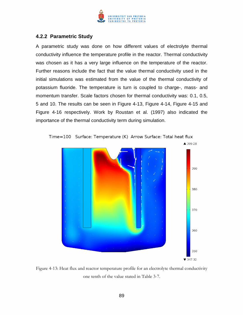
uses a set of partial differential equations to account for the momentum transfer
and bubble formation A modified Navier-Stokes that takes into account the
volume gas fraction similar to Equations 3-1 3-2 and 3-3 was used to calculate
mass transfer Bubble behaviour was modelled using a set of equation that take
into account all the forces that interact with the hydrogen bubbles as they rise
like gravity buoyancy and electrolyte flow
Figure 2-15 Cross-section of the reactor used by Espinasse et al 2006
The simulation assumes a uniform current distribution due to the large gap
between the electrodes This in turn means that the hydrogen production is also
assumed to be constant all along the cathode The flow rate was calculated using
a mean cell current the formula was not specified but it was stated that the flow
rate is related to the current density The simulation further assumes a single
bubble size of hydrogen gas produced which in turn forms the hydrogen plume
The resulting numerical calculation of gas distribution in the cell is shown in
Figure 2-16
44
Figure 2-16 Hydrogen mean gas distribution for two different current densities low on the
left and high on the right (Espinasse et al 2006)
Figure 2-16 shows a well-developed hydrogen plume in both cases with a higher
gas fraction in the case of a higher current density In both cases it is clear that
there is hydrogen ingress into the fluorine compartment It is clear that a higher
current density leads to a more hydrogen ingress
Other results from this publication relate to the effects of bubble size on the
hydrodynamics and efficiency of the reactor It was found that smaller bubbles
are more like to be entrained in the fluorine compartment leading to a drop in
current efficiency
45
254 Electrochemical Engineering Modelling of the Electrodes
Kinetic Properties during Two-Phase Sustainable Electrolysis
(Mandin et al 2009)
Industrial production of fluorine hydrogen or aluminium by electrolysis creates
bubbles at the electrodes These bubbles play a major roll on the electrochemical
and electrical properties of the electrolyte as well as having a stirring effect on
the electrolyte The goal of this publication was to better investigate the
properties of bubbles on electrolysis as bubble properties have a major influence
on the economics of electrolysis
Experiments were conducted in an electrolysis reactor described in the
publication Photographic results of bubble formation near an electrode are
shown in Figure 2-17
Figure 2-17 Bubble accumulation at 125 V around the working electrode during alkaline
water electrolysis (Mandin et al 2009)
From Figure 2-17 we can deduce the shape of a hydrogen bubble plume and
approximately estimate gas fraction The shape of the bubble plume is that of an
inverted pyramid formed due to buoyancy forces acting on the bubbles
46
255 Modeling and Simulation of Dispersed Two-Phase Flow
Transport Phenomena in Electrochemical Processes (Nierhaus
et al 2009)
Only select chapters from this thesis were studied particularly the fifth chapter
ldquoCoupling of two-phase flow and electrochemistryrdquo The reader is introduced to
the basics of electrochemistry the chapter then progresses to more advanced
concepts and fundamental laws that exist in an electrolysis cell Modelling
requirements for a representative electrochemical system are also listed
Transport equations are discussed next Equations used for mass conservation
potential field current density field in the multi-ion transport and reaction model
(MITReM) are listed The MITReM model was used by Nierhaus et al (2009) to
model behaviour in an electrochemical cell Boundary conditions for the
electrodes Insulators inlets and outlets used in the MITReM is also listed A lot
of overlap exists in the equations used by Nierhaus et al (2009) and the author
of this thesis The use of an integrated Butler-Volmer equation that does not
require the calculation of an exchange current density but still incorporates
reactive species concentration was of particular interest
The discussion continues to consider gas evolving electrodes and the effect they
have on electrolyte motion ion concentration and potential drop between the
electrodes Bubble effect on conductivity and diffusion coefficients and
correlations to calculate these parameters are discussed in some detail Bubble
formation and detachment is discussed as well as the forces that influence
bubble motion and the effect bubbles have on the electrolyte is discussed at
length
In the next section focus shifts towards the modelling procedure The software
packages used are explained their various functions and how they are integrated
into one multi-physics solver package These packages calculate the Navier-
Stokes ion-flux charge and current density distribution bubble formation and
47
bubble trajectory data The solution method and interconnectivity of all these
modules and boundary conditions are also explained
A parallel plate gas evolving reactor is modelled in the next section of the thesis
The reactor is shown in Figure 2-17 In this cell a range of ions exist in solution
Na+ SO2- NaSO- HSO- OH- and H+ all in H2O Hydrogen forms at the cathode
and oxygen at the anode The anode (top) is located downstream of the cathode
(bottom)
Figure 2-18 Parallel flow reactor as simulated by Nierhaus et al (2009)
Gas production was calculated at incremental potential differences after 2 s
Results are shown in Figure 2-19 A clear impression of bubble rise and
dispersion is obtained from the images Bubble rise due to buoyancy is
influenced by drag force induced by electrolyte movement Larger bubbles seem
to rise faster than smaller bubbles as expected
48
Figure 2-19 Gas production in a parallel flow reactor after 2 s as simulated by the Nierhaus
group
26 Summary Conclusion
As an introduction to this thesis a survey was done on a range of industrially
relevant electrolysis reactors In these reactors non-spontaneous chemical
reactions are completed with the application of a direct current to two electrodes
placed inside a conductive electrolyte medium Gas evolution metal deposition
and other industrially relevant reactors were discussed Electrolysis enabled
modern society to attain a range of materials that was impossible or extremely
expensive to produce in the past
49
Focus was then shifted to specifically fluorine electrolysis The only commercially
viable way to produce fluorine is via electrolysis of hydrogen fluoride Due to the
low electrical conductivity of the reactant gas the first cells were cooled to -50 degC
Later cells used a molten potassium acid fluoride electrolyte and become known
a high temperature cell It was found that the melting temperature of the
electrolyte can be decreased by controlling the amount of hydrogen fluoride in
solution and as a result the medium temperature cell was born and is still in use
today
Fluorine progressed from a laboratory curiosity to industrial scale production with
the discovery of nuclear fission where it is used in the uranium enrichment
process Fluorine compounds were also used during the Second World War as
an incendiary agent Today it can be found in a range of fluorine compounds
ranging from refrigerants polymer compounds the electronics industry to
specialty chemicals
As mentioned before fluorine is produced from the electrolysis of hydrogen
fluoride in a potassium acid fluoride electrolyte Hydrogen is produced as a side
product The hydrogen fluoride is produced from fluorspar reacted in sulphuric
acid Following electrolysis the gaseous products must be purified to remove any
entrained hydrogen fluoride
The electrolysis process is discussed in much detail Detail is given on the
electrolyte its manufacture and physical properties The carbon anode and
anode phenomena is discussed specifically polarisation and overvoltage
phenomena The cathode separator skirt and cell body are discussed next
Electrochemical concepts such as reversible and working voltage are discussed
in the subsection that follows Next heat production specifically is discussed
within the cell followed by a subsection on other fundamental transport and
modelling equations The section describing a fluorine cell is concluded with a
discussion on the gasses produced during electrolysis
50
The literature review of this report is concluded with a study of published fluorine
electrolysers Valuable knowledge was gained from these works knowledge
used to aid in the set-up of the model presented later in this contribution Due to
the incompletion of the experimental reactor the model could not be compared to
experimental results The modelling approach was consequently evaluated by
comparing published fluorine electrolysis simulations to simulations done by the
author on COMSOL Multiphysicsreg
Two papers were chosen for this the first by Roustan et al (1997) where the
charge heat and momentum transfer in a lab-scale fluorine electrolyser was
modelled and compared to experimental results The second was a publication
by Espinasse et al (2006) where two phase bubbly flow was modelled in a
fluorine electrolyser Two phase flow results were compared to results found in
this paper Other works included a paper published by Hur et al (2003) where
bubble flow inside a fluorine electrolyser was modelled Knowledge gained here
served as a warning of the danger of small bubbles becoming entrained in the
electrolyte flow which could lead to explosive recombination of product gases
The contribution by Mandin et al (2009) was studied to get a rough idea of the
shape of a hydrogen bubble in an electrolyte The bubble shown is that of
hydrogen in an aqueous medium and does not give an accurate portrayal of a
hydrogen bubble in a potassium acid fluoride electrolyte Lastly parts of the
thesis of Nierhaus et al (2009) were studied to gain more knowledge on the
workings of two phase simulations of electrolysers
The knowledge gained from the lliterature review was used in later parts of this
thesis to aid in the design of the simulation and interpret results gained from the
simulation Looking at published works it was clear that a fully coupled model is
absent from literature The review further revealed ways in which the model
presented in this report could be improved upon
51
3 Model Development
31 Reactor Description
A cross-section of the electrolysis reactor is shown in Figure 3-1 The reactor
construction material is mild steel The anode is non-porous carbon and the
cathodes are mild steel Gasses produced during electrolysis are separated by a
mild steel separator skirt The skirt (which has been electrically isolated) is
submerged by 15 cm into the electrolyte this ensures that a very small area of
the skirt is available to produce hydrogen if bipolarisation does occur
Figure 3-1 Cross-section of the electrolysis reactor
32 Model Description
The model is based on a laboratory scale experimental 2F -electrolysis reactor
built at the University of Pretoria constructed to better understand the inner
workings of the industrial scale 2F -electrolysis reactors at NECSA Industrial
reactors decompose HFKF 2 on a continuous basis re-supplying HF to the
reactor as HF is decomposed by electrolysis into 2H and 2F The laboratory-
52
scale reactor works as a semi-batch reactor ie there is no re-supply of HF as it
is consumed in the electrolysis reaction
Modelling was conducted using the software package COMSOL Multiphysics
For the sake of reproducibility the modelling procedure will be explained in a
stepwise fashion corresponding to the method employed during modelling with
the software package
The cross sectional-area of the reactor that was modelled is shown in Figure 3-2
Figure 3-2 Model dimensions
53
The COMSOL model only includes the reactor contents up to the electrolyte level
and uses the electrolyte properties as specified in Table 3-7 The electrodes
were also modelled the anode material was modelled as carbon and the cathode
as mild steel (properties indicated in Table 3-7)
The following physical and chemical transfer solutions were selected and
reconciled with the information provided in the literature review
321 Momentum Transfer
Flow induced inside the reactor is modelled by Equation 3-1 Equation 3-2 and
Equation 3-3 the momentum transport continuity and laminar bubbly flow
equations respectively These equations are found in the ldquoLaminar Bubbly Flowrdquo
physics node of the software suite used
FgIuuuPut
ulll
T
llTlllll
l
ll
3
2 3-1
0 lu
3-2
0
ggg
ggu
t
3-3
Subscripts ldquo l rdquo and ldquo g rdquo denotes the gas and liquid phases
Using these equations modelling of mixtures and gasses can easily be achieved
by solving for the averaged volume fraction occupied by each of the two phases
rather than tracking each bubble in detail This procedure assumes two different
velocity fields one for each phase The following assumptions are adhered to
(COMSOL Multiphysics (a) 2010 Espinasse et al 2006 Loth et al 2006)
54
The gas density is negligible compared to the liquid density
The motion of the gas bubbles relative to the liquid is determined by a
balance between viscous drag and pressure forces
The two phases share the same pressure field
Gas volume fraction is less than 01
Flow is induced in the reactor due to the following interactions
Ionic migration due to concentration gradients
Ionic migrations due to electric field interactions
Convection due to gas bubble formation at the electrodes
Convection caused by temperature gradients due to heating
Laminar bubbly flow (Reynolds numberlt01) was assumed for the hydrogen
bubbles and the assumption was later justified by calculation Additionally it was
assumed that the bubbles are small and perfectly spherical Therefore Stokes
law was applied to calculate the terminal velocity of hydrogen gas bubbles
(Talalia 2007) An estimated bubble size of 1 mm was used during calculations
(Espinasse et al 2006) It should be noted that fluorine bubbles are long
lenticular bubble that do not detach from the anode and therefore Stokes law will
not give valid terminal velocity results
The largest bubble terminal velocity ( 2H at 363times10-4 1 sm ) had a Reynolds
number of 2421times10-4 a value less than 01 (justifying the earlier assumption)
and validating the use of laminar bubbly flow for bubble movement
The reader should take note that the physical properties of only one gas
(hydrogen) was used to model both product gasses in the simulation this is due
to lack of data concerning both gasses in the reactor and an inability of the
modelling software to model two gasses in a two-phase problem To overcome
this shortcoming both gasses were modelled as Hydrogen Seeing as the two
55
gasses have massive differences in physical particularly bubble properties and
behaviour some modifications had to be made to the gas produced at the anode
The flow rate of fluorine was adjusted with a constant factor (01) This ensures
that the upward moving effect of the fluorine bubbles on the anode is included in
the simulation but that the fluorine bubble retains its key properties (slow moving
lenticular bubbles that stick to the anode and slowly move to the electrolyte
surface These bubbles do not break away from the electrode surface and are
propelled by buoyancy forces These qualities are adequately retained as can be
seen in the results section (Hur et al 2003 Rudge 1971) In other works by
Roustan et al (1997) Hur et al (2003) and Espinasse et al (2006) the effect of
the fluorine bubbles were either completely neglected or compensated for as a
moving boundary
322 Heat Transfer
Heat transfer due to convection and conduction inside the reactor is modelled
using in Equation 3-4 below found in the ldquoHeat Transferrdquo physics module of the
software package (COMSOL Multiphysics (b) 2010 Ccedilengel 200674-76) Heat
generation due to viscous heating was ignored The walls of the reactor where
temperature was specified will be the only heat sink during the modelling
procedure The remaining reactor walls will additionally remove heat via radiation
to ambient atmosphere and the electrolyte level will remove heat via convection
TuCQTkt
TC pp
)( 3-4
The internal source of heat in Equation 3-4 is heat generation due to resistive
losses or Ohmic heating in the electrolyte seen in Equation 3-5 (Rudge 1971
34) This equation is used throughout the entire electrolyte domain during
simulation Heat generated within the electrodes will be predicted using Equation
2-7
56
ieRV d
EiiQ 1
100
100812
3-5
323 Charge Transfer
The chemical reaction (electrolytic decomposition of the electrolyte into F2 and
H2) is induced by electric potential predicted by Equations 3-6 (Laplace Equation)
which predicts the primary current distribution and adheres to the assumption of
Equation 3-7 The Laplace Equation is the default equation used in the ldquoElectric
Currentsrdquo physics node of COMSOL Multipysics
0)( d 3-6
02 3-7
The physics model used in COMSOL assumes that the electric field only varies
in two dimensions (xy-plane) and is constant in the z-direction By implication this
means the electric filed is tangential to the xy-plane (COMSOL Multiphysics (c)
2010 Roustan et al 1997)
324 Mass Transfer
Mass transfer inside the reactor is modelled using Equation 3-8 (Newman 1991
194 Welty et al 2001 COMSOL Multiphysics (d) 2010)
iiiimiii
i ruCFCzCDt
C
)(
3-8
The ldquoTransport of Diluted Speciesrdquo physics node in the software suite was used
because the reactive solvent concentration is approximately 60 (molar) of the
57
solution and the solute will not be re-supplied during experimentation further
diluting the reacting species The three species assumed to be in solution are
given in Table 3-1 The electrolyte dissociation reaction is given by Equation 3-9
(Crouse 2010)
22 HFHFKHFKF 3-9
Table 3-1 Chemical species assumed to be present during electrolytic production of
hydrogen and fluorine (Crouse 2010)
Species Charge Number iz
K +1
2HF -1
HF 0
Dilute species flux at the electrodes was further modified to include the effect of
bubbles near the electrode surface This was achieved by finding the product of
the calculated diluted species flux and the calculated liquid fraction at the specific
point in the electrolyte
3241 Electrode Reactions
Electrode reactions occurring in the reactor are assumed to be Equations 3-10
and Equation 3-11 (Groult 2003) Reaction 3-10 occurs at the anode and
reaction 3-11 at the cathode
eFHFHF 221
2 3-10
221
22 HHFeHF 3-11
58
Equations 2-7 2-8 amp 2-9 are used to predict gaseous production rate of both
product gasses These consumption rate equations are stoichiometrically
adjusted to predict production rate of reactant species and product gasses at the
electrode surfaces The reaction rate was calculated with data supplied by
Crouse 2010 (2010) The production rate of fluorine is further adjusted by a
fractional value (01) Fluorine bubbles tend to stick to the electrode and move up
the anode at low speed therefore a detached bubble model for fluorine would
overestimate the stirring effect of fluorine in the cell
325 Starting Conditions
The starting conditions in the reactor are given in Table 3-2
Table 3-2 Starting conditions used in the model
Transfer Process Description
Momentum Transfer Velocity equals zero
Heat Transfer Reactor temperature equals 80 degC
Charge Transfer
Mass Transfer
Cell Voltage equals 0 V
Reactive species concentration equals 1000 molm-3
326 Boundary Conditions
Boundary conditions used in the model are given in Table 3-3 (Momentum-
Transfer) Table 3-4 (Heat-Transfer) Table 3-5 (Charge-Transfer) and Table 3-6
(Mass-Transfer)
It should be noted that the reactor wall boundary conditions for heat- (radiation)
and charge transfer (insulation) are chosen to correspond to the boundary
conditions that would be valid on the outside of the reactor The values were
chosen as such due to the low thickness of the wall combined with its high
59
thermal and electrical conductivity This estimation simplifies the model as only
one domain material is now in use for the external boundaries
60
Table 3-3 Boundary conditions for momentum transport
Boundary Boundary Condition Description Equation
Electrolyte
level
Liquid boundary condition slip
Gaseous boundary condition gas
outlet
Acts as a gas outlet and allows liquid slip 0
t
ul
ggg
gu
t
u
Anode surface Liquid boundary condition no slip
Gaseous boundary condition gas flux
Allows gas production according to specified
reaction rate AR No liquid flow
0lu
Ag
gRn
t
u
Cathode
surface
Liquid boundary condition no slip
Gaseous boundary condition gas flux
Allows gas production according to specified
reaction rate CR No liquid flow 0lu
Cg
gRn
t
u
All other
boundaries
Liquid boundary condition no slip
Gaseous boundary condition no gas
flux
Allows neither gas or liquid flow both without slip 0
t
ui
61
Table 3-4 Boundary conditions used to model heat transfer within the reactor
Boundary Boundary Condition Description Equation
Walls in contact with heatingcooling jacket Temperature specified Wall temperature set to wT a
constant 80 degC
wTT
Walls in contact with ambient air Ambient radiation Heat flux set to radiate to
ambient conditions
wTT
Top of electrolyte Convective cooling Heat flux set to convective
cooling
wTT
All other boundaries Thermal insulation No heat flux allowed 0)( Tkn
Table 3-5 Boundary conditions used to model charge transfer within the reactor
Boundary Boundary Condition Description Equation
Anode Inward current
density
Current density Ai as determined by the Butler-Volmer equation An iin
Cathode Inward current
density
Current density Ci as determined by the Butler-Volmer equation Cn iin
All other
boundaries
Electric insulation No current flow allowed 0 nin
62
Table 3-6 Boundary conditions used to model mass transfer within the reactor
Boundary Boundary
Condition
ValueExpression Equation
Anode Dual mass
flux
Reactive species HF flows into electrode and
2HF out of
electrode as defined by AR
Aiii RnuCCDn )(
Cathode Inward
current flow
Reactive species
2HF flows into electrode and HF out of
electrode as defined by CR
0)( uCCDn iii
All other
boundaries
Mass flow
insulation
No mass flow allowed Ciii RnuCCDn )(
63
327 Constants
Constants used during modelling are given in Table 3-7
Table 3-7 Model constants
Constant Description Value Reference
0pC Constant pressure heat capacity at 25 degC 108 1-1kg KJ Rudge 1971
bd Average bubble diameter 1 mm Espinasse et
al 2006
HFD Mass transfer coefficient for HF 82 times 12510 sm Estimated
2HF
D Mass transfer coefficient for
2HF 3 times 12510 sm Estimated
E Current efficiency 95 Rudge 1971
F Faradayrsquos constant 96485 1molC
g Gravitational acceleration 819 2 sm
ctk Thermal conductivity of carbon 150 11 KmW Estimated
etk Thermal conductivity of electrolyte 251 11 KmW Estimated
stk Thermal conductivity of steel 544 11 KmW Estimated
Ak Effective rate constant for
2HF 1 1 sm Estimated
Ck Effective rate constant for HF 1 1 sm Estimated
rtrP _ Atmospheric pressure inside the
electrolysis cell
86 kPa Crouse 2010
gR Ideal gas constant 3148 11 KmolJ
0T Starting temperature of electrolyte 15353 K Crouse 2010
wT Wall temperature of electrolysis cell in
contact with heating jacket
15353 K Crouse 2010
A Anode electron transfer coefficient 050 Newman
1991 17
64
C Cathode electron transfer coefficient A-1 050 Newman
1991 17
Thermal expansion coefficient of
electrolyte
117 times 410- 1C Rudge 1971
r Relative permittivity 9 Estimated
Cell electric potential 12 V Crouse 2010
RV Reversible cell voltage 92 V Rudge 1971
A0 Electric potential at anode 92 V Crouse 2010
C0 Electric potential at cathode 0 V Crouse 2010
l Liquid (electrolyte) viscosity (assumed
constant)
01130 sPa Espinasse et
al 2006
g Gas viscosity (assumed constant) 0010 sPa Crouse 2010
c Electrical conductivity of carbon 3 times310 1mS Crouse 2010
e Electrical conductivity of electrolyte 676 1mS Crouse 2010
s Electrical conductivity of steel 4 times610 1mS Crouse 2010
g Gas molar density 4122 1molkg
0 Density of electrolyte at 25 degC 2000 3mkg Crouse 2010
328 Expressions
Expressions used during modelling are given in Table 3-8
Table 3-8 Model expressions
Expression
Name
Description Expression Reference
pC Temperature
dependent
heat capacity
TCC pp 0028400
Rudge
1971
65
Q Total heat
production
100
9510081291 iViQ
Rudge
1971
AR HF
consumption
at anode
AA iF
R1
Crouse
2010
CR
2HF
consumption
at cathode
CC iF
R2
Crouse
2010
0i Exchange
current
density
50505050
02
HFHFac CCkFki Newman
1991 195
Ai Anode
current
density
s
g
Cs
g
AA
TR
F
TR
Fii
expexp0
Newman
1991 194
Ci Cathode
current
density
s
g
Cs
g
AC
TR
F
TR
Fii
expexp0
Newman
1991 194
Electrolyte
density
1
0 25exp
CT Rudge
1971 10
As Anode
surface
overpotential
As A0 Heitz amp
Kreysa
1986 101
Cs Cathode
surface
overpotential
Cs C0 Heitz amp
Kreysa
1986 101
329 Mathematical Solution
The Finite Element Method (FEM) was used for the calculation of the solution of
the mathematical model The FEM was originally developed to solve problems in
civil engineering but is now used for approximation of mathematical solutions to
66
Partial Differential Equations (PDEs) in many areas of applied mathematics
(Burden et al 2005 721)
A big advantage that the FEM has over the Finite Difference Method (FDM) is
that irregular boundaries can be handled more easily FEM makes use of the
fundamental result of the calculus of variations which states that the solution of
the PDE under consideration is also the functional that minimises a functional
ie a function of a function (an integral particular to the PDE) within the region of
solution Irregular shaped boundaries and boundary conditions involving
derivatives are approached by including boundaries as integrals of the function
that is being minimised This results in the solution construction procedure being
independent of the particular boundary conditions of the problem (Burden and
Faires 2005 721-722)
Triangles squares or any regular shape are used to divide the region of the PDE
into sections or elements This collection of elements is called ldquothe meshrdquo The
set of function used to approximate the shape is commonly a set of linear or bi-
linear polynomials of fixed degree in x and y The polynomial functions must be
pieced together so the resulting function is continuous and can be integrated in
the first or second derivative over the entire problem region A typical linear
polynomial used with triangular elements is given by Equation 3-11
cybxayxf )( 3-11
The expressions are used to indicate how the value of a variable relates to that
variable value at another point (or node) connected by the expression A sum of
these relations weighted by the nodal values is approximated as a solution to the
problem The equations of the weighted sum are then minimized Rapid changes
in variables are more accurately indicated with smaller mesh elements (Burden
and Faires 2005 722)
67
3291 Solution Method
MUltifrontal Massively Parallel sparse direct Solver (MUMPS) was used as a
direct solver with a memory allocation factor of 12 Pivoting was used with a
pivoting threshold of 01 A constant damping factor of 1 was used The
maximum allowed iterations were set to 5 All solutions were done without the
use of inconsistent stabilisation but rather with consistent stabilisation
To solve the charge transfer problem (Calculation A) cell potential (Ecell) was
used as a changing parameter in a separate stationary parametric sweep
calculation step The value of Ecell was incrementally increased form 3 V to
12 V This allowed the simulation to use the lower (and easier to solve) value of
Ecell as a starting point for the next (higher value)
The final 12 V value of Ecell was then used as a starting value input to a time
dependent calculation (Calculation B) In this second calculation the momentum-
and heat-transfer phenomena were solved based on the constant charge
transfer values supplied Momentum and charge-transfer was chosen due to their
coupling and large amounts of interaction
A third calculation (Calculation C) was attempted where the final results of
Calculation B were used as initial input values In this calculation the mass-
transfer in the reactor was calculated using the values calculated in
Calculation B Mass-transfer was calculated last as it is coupled with all the other
transfer modules and presents a significant challenge to the solver
It is clear that final calculation (Calculation D) was needed to firstly determine
time dependent values of all transfer phenomena and to also ensure transient
coupling between all transient transfer regimes In this calculation charge- mass-
momentum and heat-transfer was calculated It was chosen last as it is the
largest and most complex set of equations to solve where coupling occurs
between all transfer modules In Calculation C stationary values of
68
charge-transfer and transient values of heat momentum- and ion-transfer was
used to solve for transient values of mass transfer To achieve calculation D final
time-step results of Calculation C was used as an initial value input Results of
Calculation D are presented in the Results and Discussion section Calculation D
includes fully coupled time dependent ion-transfer results
3292 Meshing
Two meshes were used during the solution of this problem The first (henceforth
referred to as Mesh I) was used in Calculations A-C and can be seen in Figure
3-3
Figure 3-3 Mesh I used for calculations A-C
69
Mesh I has 11398 triangular mesh elements and was set up by the user Smaller
mesh elements were used around perceived complex points in the system
Statistics on Mesh I can be seen in Figure 3-4
Figure 3-4 Detailed statistical data for Mesh I
A very fine or ldquofinerrdquo physics controlled mesh in the software suite settings was
used for the solution of Calculation D this resulted in 20621 triangular mesh
elements This mesh will be referred to as Mesh II The mesh was further refined
around the electrodes and separator skirt where there are very complex
interactions occurring between the various transfer processes specifically the
70
high current density concentrations This specific mesh configuration was used to
aid in convergence The mesh can be seen in
Figure 3-5 Meshing framework of fluorine cell (Mesh II)
Notice the extremely fine mesh around the electrodes this was used as the finer
mesh is more suited to handle complex boundary conditions It also aids in
convergence Notice the rectangular mesh elements around the electrodes and
outer walls These so-called ldquoBoundary-layerrdquo mesh elements are specifically
suited to complex coupled boundary layered conditions and help the model to
converge Further statistics concerning Mesh II is presented in
71
Figure 3-6 Detailed mesh statistics for Mesh II
32921 Mesh Dependency
As an additional step to ensure the reliability of the solution a further study was
conducted In FEM simulations it is possible to obtain a solution to a problem that
only solves for a specific mesh This is called a mesh dependent solution As a
measure to prevent possible mesh dependent solutions or unwanted error
propagation two different meshes (Mesh I and Mesh II) were used during
calculation Mesh I was used for calculations A B and C while Mesh II was used
for Calculation D Further refinementconvergence test were also done
72
Mesh I was refined by an entire order to roughly double the number of mesh
elements Mesh I was chosen as this is the mesh used to ramp up the applied
reaction voltage in Calculation A this is potentially troublesome as it could force
the solution to converge from a previous solution This in could result in a
memory effect which could diverge the simulated solution from the real solution
Noise can accumulate and becomes especially troublesome in sensitive areas
such as the tips of electrodes As shown by Caire et al (2002) the current
distribution in any electrolyser is very sensitive to mesh quality Calculation A
was repeated with the smaller sized mesh (over 220000 mesh elements) and
results were practically identical The differences are illustrated in Figure 3-7
using the COMSOL Multiphysics feature that allows data sets to be joined and
then compared
Figure 3-7 Comparative graphic of electric potential for two different meshes
73
Figure 3-7 shows the electric potential at a cell voltage of 12 V for the refined
mesh of over 220000 mesh elements subtracted from the original mesh (Mesh I)
at a cell voltage of 12 V A refinement in mesh in the direct solver used by the
author results in a third power increase in calculation time therefore due to the
lack of a cluster only Calculation A was completed with a finer mesh
A second study was conducted where the allowed error was decreased from its
previous value (1e-5) to a lower value (1e-7) on the original rougher mesh
Calculation A was then repeated and practically identical results were found It
was therefore concluded that the solution is very near to an analytical solution
and not ldquoforcedrdquo
Lastly Calculation D was repeated three times on consecutively finer meshes to
check for convergence This was achieved in all three cases These results are
not shown in this report
3293 Computing
An Intel I7 CPU 870 with 293 GHz and 16GB RAM on Windows 7 64bit
operating system requires around just over 30 min to compute Calculation D
Calculation A solves in just over 120 s Calculation B in just over 80 s
Calculation C in 27 s Calculation D requires Calculation times were significantly
improved on the latest version of COMSOL Multiphysics (version 42a) As a
reference in version 42 Calculation D took well over 16 hours Once Calculation
A-C have been completed only Calculation D needs to be run for minor changes
in the model setup
Mesh dependency studies increased the required calculation time due to the
increase in the number of mesh elements Calculation times for Calculation A
when on the refined Mesh I took just over 4 hours While the calculation times for
Calculation A where the allowable error was decreased increased calculation
74
time to just over 150 s Mesh dependency studies done on Calculation D
increased calculation time to exponentially for each incremental decrease in
mesh size
75
4 Results and Discussion
From Figure 4-1 it is clear that after an initial rapid rise the average liquid
velocity reaches an asymptotic value after a relatively short period It was
therefore be assumed that the hydrodynamic conditions within the reactor will not
change much after 100 s as a quasi-steady-state condition was reached Work
by Espinasse et al assumed that a quasi-steady-state is reached once the
hydrogen plume has fully formed Gaseous movement induces stirring in the
electrolyte and remains the major contributor to electrolyte movement throughout
reactor operation Therefore once this flow pattern has been established it can be
assumed that flow conditions will not change much as time progresses
Figure 4-1 Average liquid velocity inside the reactor over time
76
The value of a transient simulation further lies in knowledge gained in the startup
period of a reactor True steady state is also of importance but non-existent in a
batch reactor Results will therefore focus on the reactor conditions at 100 s
Transfer phenomena where significant or interesting change did occur will be
shown in 11 s intervals
41 Momentum Transfer
The simulation gave the following momentum transfer results Gaseous
movement inside the reactor can be seen in Figure 4-2 The colour scale on the
right indicates gaseous velocity in meters per second Warmer colours indicate
higher velocities The vector arrows indicate the direction of the gaseous flow at
the arrow origin The size of arrows is proportional to the velocity of the gas at
the point of origin
From Figure 4-2 it is clear that gas is produced at both electrodes The product
gasses move away from the electrodes and upwards and out of the reactor This
upward motion contributes to the liquid phase movement inside the reactor The
reader should however note the presence of vector arrows all over the reactor
does not necessarily indicate the presence of a gas at that point but does in fact
indicate the path a gaseous element would take if present at that point The
indicated velocity at this point is mainly a function of buoyancy and a bubble
placed at that point would move at the indicated velocity in the indicated
direction
77
Figure 4-2 Gas phase velocity inside the electrolysis reactor
Liquid phase movement can be seen in Figure 4-3 The colour scale on the right
represents liquid phase velocity inside the reactor warmer colours represent
higher velocities Arrows indicate direction and is proportional to velocity at the
arrow starting point
The liquid movement induced by gaseous (specifically hydrogen) movement is
evidenced by the swirling liquid phase eddy between the separator skirt and the
left of the cathode at the top right of the reactor The downward motion of the
liquid eddy in turn influences gas phase movement shown by the reduced gas
phase velocity where the liquid moves downward The downward liquid motion
induces stirring in the reactor This same eddy has the effect of causing stirring
throughout the reactor The downward liquid torrent extends and moves down
toward the bottom of the reactor where it starts moving upward once more This
78
upward movement is aided by the liquid movement induced by fluorine gas
upward motion along the anode It should be noted that this fluorine flow is in fact
hydrogen flow that has been altered to allow the inclusion of the stirring effect
fluorine bubbles could have in the reactor The stirring eddy then turns around
once more as it reaches the top of the reactor and joins up with the liquid eddy
induced by hydrogen gas movement
Figure 4-3 Liquid phase velocity inside the reactor
The relatively low levels of electrolyte movement in the space between the
reactor walls and electrodes indicate that the reactor size can possible be
reduced which will in turn reduce costs Alternatively the distance between the
electrodes can be increased to further aid in the prevention of product gas
recombination The fluid flow lines are presented in Figure 4-4
79
Figure 4-4 Liquid phase velocity streamlines plot and liquid flow arrows inside the simulated
reactor
Figure 4-4 clearly shows the dead volumes and eventual bubble recirculation
paths within the reactor These will be discussed in more detail following the
presentation of Figure 4-5 Liquid velocity vector arrows and gas fraction in the
reactor are shown in Figure 4-5 Warmer colours indicate higher gas fractions
and colder colours indicate a low gas fraction
Figure 4-5 shows a well-developed hydrogen plume and detachment from the
cathode occurs as expected The fluorine plume on the other hand does not
detach from the anode This is to be expected as fluorine bubbles form long
lenticular bubbles that tend to move slowly up along the electrode Very little
hydrogen migration into the fluorine section is observed therefore the chance of
explosive recombination of product gasses is very low The liquid flow pattern
80
does suggest that recombination is possible but the gas velocity profile suggests
that the bubble will leave the reactor as soon as it gets to the top This is also
good news from a productivity standpoint as fewer product gases are lost and
less purification of product streams will be required
Figure 4-5 Gas phase fraction in the reactor
It should however be noted that if bubbles become sufficiently small they may be
entrained in the liquid velocity flow path This effect was demonstrated by Hur et
al (2003) If this effect does occur it could in fact lead to explosive recombination
of product gases Bubbles in this simulation are all of 1 mm size so buoyancy
force should dominate convection in terms of bubble trajectory
81
411 Time Progression
Initially there is little movement in the reactor but as time goes by the convection
due to gaseous flow in the reactor temperature fluctuations and migration of
dissolved species due to electric field migration results in eddying motion in the
reactor This can be observed in the time progression plots of Figure 4-6 Figure
4-7 and Figure 4-8 From these plots it becomes clear that convection is the
major source of movement within the reactor As mentioned earlier the electrolyte
motion in the reactor is induced by gaseous flow This flow pattern development
can be seen in the time progression plots that follow
82
Figure 4-6 Gaseous phase velocity time development sequence
83
Figure 4-7 Liquid phase velocity time development sequence
84
Figure 4-8 Gaseous phase volume fraction time development sequence
85
42 Heat Transfer
The temperature distribution inside the reactor is shown in Figure 4-9 the colour
scale on the right indicates temperature in kelvin warmer colours represent
higher temperatures and vice versa
Figure 4-9 Heat flux and reactor temperature profile
Ohmic heating is the major source of reactor heating as reflected by the current
density concentration seen in Figure 4-17 A lot of heat is generated at the
bottom of the electrodes as these are the points where the highest current
density exists and therefore the most heat is generated here The stirring effect
of the moving liquids induced by the moving gases and shown by the vector
arrows are visible in Figure 4-9 These arrows represent total heat flux inside the
reactor The size of the arrow is proportional to magnitude of the heat flux and
86
the arrow points in the direction of heat flux at the arrow origin The heat flux
arrows indicate that convection as the dominant heat transfer contributor as heat
flux takes up the same ldquoshaperdquo as that of the electrolyte motion The cooling
effect of the reactor walls and radiation heat loss can also be seen as the
temperature decreases closer to the cooled wall and bottom of the reactor
The heat flux within the reactor is further broken down in to conductive (Figure
4-12) and convective (Figure 4-12) heat flux to supply additional information
concerning heat flux and its contributing components Super-imposed on both
images are arrow that indicate direction and magnitude of flux
Figure 4-10 Conductive heat flux within the reactor
From Figure 4-12 it is clear that heat is removed at the sides of the reactor via
the cooled walls and some via radiation from the bottom of the reactor Although
87
convection from the top of the electrolyte was included in the model the effects
appear negligible
Figure 4-11 Convective heat flux within the reactor
Looking at the magnitude of the heat flux vector in Figure 4-12 it can be
concluded that convection is the major contributor to heat transfer within the
reactor with a seven hundred times higher maximum flux than conduction
421 Time Progression
The progression of temperature in the reactor can be seen in Figure 4-12 The
time progression plots show how the temperature within the reactor changes
from the starting temperature of 80 degC to the maximum temperature shown due
to Ohmic-heating The rise in temperature is initially fast but slows as time
passes
88
Figure 4-12 Temperature time progression sequence
89
422 Parametric Study
A parametric study was done on how different values of electrolyte thermal
conductivity influence the temperature profile in the reactor Thermal conductivity
was chosen as it has a very large influence on the temperature of the reactor
Further reasons include the fact that the value thermal conductivity used in the
initial simulations was estimated from the value of the thermal conductivity of
potassium fluoride The temperature is turn is coupled to charge- mass- and
momentum transfer Scale factors chosen for thermal conductivity was 01 05
5 and 10 The results can be seen in Figure 4-13 Figure 4-14 Figure 4-15 and
Figure 4-16 respectively Work by Roustan et al (1997) also indicated the
importance of the thermal conductivity term during simulation
Figure 4-13 Heat flux and reactor temperature profile for an electrolyte thermal conductivity
one tenth of the value stated in Table 3-7
90
Figure 4-14 Heat flux and reactor temperature profile for an electrolyte thermal conductivity
half of that stated in Table 3-7
Results from the parametric study show that the maximum temperature as well
as the heat distribution in the reactor varies with a change in thermal
conductivity It is however noted that even an increase in thermal conductivity by
a factor 10 only changes the maximum reactor temperature by less than 30 K
The same can be said for lowering the conductivity by a factor of 10 a maximum
temperature increase of only 13 K An increase in thermal conductivity leads to a
more symmetric temperature distribution
91
Figure 4-15 Heat flux and reactor temperature profile for an electrolyte thermal conductivity
five times higher than stated in Table 3-7
92
Figure 4-16 Heat flux and reactor temperature profile for an electrolyte thermal conductivity
ten times higher than stated in Table 3-7
43 Charge Transfer
The normal current density distribution inside the electrolysis reactor can be seen
in Figure 4-17 The colour scale represents current density in Amiddotm-2 warmer
colours indicate higher densities This figure also contains streamlines indicative
of electric field lines between the electrodes
93
Figure 4-17 Current density distribution and electric field streamlines
High current densities appear on sharp corners of the electrodes especially high
values are visible on tips between the two electrodes Current density is also very
high on the tip of the separator skirt The tip of the skirt has such a high current
density due to the fact that the charged ions flow around this point to travel
between electrodes These are major heat sources during electrolysis
Current density variation along the anode is shown in Figure 4-19 It should be
clarified at this point that ldquoArc-lengthrdquo is in fact the distance travelled along the
anode (and cathode) The ldquoArc lengthrdquo axis starts on the top left of the anode and
ends at the top right This is further explained in the underlying image (Figure
4-17)
94
Elec
tro
de
α
β γ
δ
Arc length
α β γ δ
Figure 4-18 Graphical explanation of ldquoArc-lengthrdquo as used in underlying figures
95
Figure 4-19 Anode current density variation along the electrode
From Figure 4-19 it is clear that the current density is exceptionally high at the
tips of the electrode This caused some difficulty during the mathematical solution
procedure The current density spikes serve as a virtual discontinuity when
moving between mesh nodes making it difficult for the Newtonian solver to find a
solution The problem was overcome by refining the mesh around the high
current density areas and by decreasing the size of steps taken by the solver In
reality these current density spikes can lead to electrode degradation in the
reactor The mirror of this image (Cathode Current Density Variation) is shown in
Figure 4-20 In Figure 4-20 the ldquoArc Lengthrdquo axis starts on the top left of the
cathode and ends at the top right
96
Figure 4-20 Cathode current density variation along the electrode surface
Figure 4-21 shows the electric potential and electric potential contour lines within
the electrolyte The colour scale indicates electric potential in V warmer colours
indicate higher voltages
97
Figure 4-21 Electric potential plot
Electric potential drops linearly from the anode to the cathode from 91 V and 0 V
as expected This result corresponds to the potential change expected from the
literature Literature however shows that the potential drop is in fact not linear
Boundary affects such as bubbles causes a large potential drop due to the low
conductivity of the gaseous phase resulting in an exponential potential drop over
these bubbles on the boundaries
The bending of the electric potential contour lines along the separator skirt
corresponds to the electric current density field lines that bend around the skirt
98
44 Mass Transfer
HF concentration in molmiddotm-3 is shown in Figure 4-22 the colour scale shown
indicates high HF concentrations at warm colours and low concentrations at cold
colours The vector arrows indicate direction- and the size of the arrows indicate
magnitude of flux at the arrow origin
Figure 4-22 Dissolved hydrogen fluoride flux and flux vectors
HF is produced at the anode and consumed at the cathode The concentration
gradient due to consumption at the cathode is a contributor to flux in the form of
diffusion From the scale-bar on the right it is clear that more HF is consumed
than produced as was predicted by the electrode half-reactions (Equation 3-8
99
and Equation 3-9) From Figure 4-22 it is evident that the secondary contributors
to flux are convection and migration due to electric field
HF2- ion-flux and concentration are shown in Figure 4-23 Arrows size indicates
flux magnitude at arrow origin and arrow directions indicate flux direction
Concentration is in molmiddotm-3 and warmer colours represent higher concentrations
Figure 4-23 Hydrogen difluoride anion-flux
The HF2- ion is produced at the cathode and consumed at the anode This is
reflected in Figure 4-23 The concentration gradient indicates ion-flux from the
cathode to the anode as expected Convection is evident as the major contributor
to ion-flux in the simulation with diffusion due to concentration gradient and
migration due to electric field acting as secondary contributor
100
441 Time Progression
Figure 4-24 and Figure 4-25 shows the time dependent development of the
hydrogen fluoride and hydrogen difluoride dissolved species respectively It is
clear when looking at Figure 4-24 and Figure 4-25 that initially there is
consumption and formation at both electrodes The gas-phase induced
electrolyte movement is major contributor to mixing of diluted species Other than
the formation of a clearly defined mixing pattern within the reactor not much else
changes except the diluted species concentrations The change in reactant
concentration relative to the starting value is extremely low The quasi-steady
state assumption was therefore not violated
101
Figure 4-24 Time dependent representation of HF concentration over time
102
Figure 4-25 Time dependent representation of HF2- concentration over time
103
45 Simulations of Published Results
This section contains the results of the authorsrsquo attempts to simulate published
results Simulations used parametric data if available in a publication
Assumptions were made where parametric data was unavailable Specialised
correlations and equations used in published works that could not be reproduced
were supplemented with the modelling procedure as described in section 32 of
this report
451 Modelling coupled transfers in an industrial fluorine
electrolyser (Roustan et al 1997)
A COMSOL Multiphysics simulation of the fluorine electrolyser published by the
Roustan et al (1997) was also completed by the author Dimensions supplied
were used as well as parameters supplied Not all data required for simulation
were supplied in the publication The missing information required for simulation
was taken from Table 3-7 and Table 3-8 as used for own work Extracted
expressions from these tables are presented in Table 4-1 Parameter values that
were unavailable or unusable when extracted are shown in Table 4-2
Table 4-1 Extracted expressions as used in COMSOL simulation
Extraction Description Expression
Non-uniform current
distribution
Current density along the electrodes
was described by the Butler-Volmer
equation Data concerning the uniform
current density used in the publication
was unavailable
Equation 2-8
Total heat
production
The expression used in the publication
to describe total heat production
requires a value for the thermo-neutral
voltage of the cell this was not supplied
and a value was therefore extracted
Equation 3-5
104
Table 4-2 Assumed parametric values as used in COMSOL simulation
Assumed value Description Value
Exchange current density A constant value was assumed over the
anode
12 2mA
Cooling coil temperature Data concerning the cooling capacity of
the coils were unavailable a constant
value for coil temperature was assumed
325 K
The resulting equipotential curve is shown in Figure 4-26
Figure 4-26 Equipotential curves from the COMSOL simulation of the cell as published by
Roustan et al (1997)
105
When comparing the equipotential curves to those obtained in Figure 2-7 by
Roustan and co-workers a similar voltage drop between the electrodes can be
observed The shape of the curves are nearly identical between the electrodes
but differs for the rest of the cell A possible explanation could be that the
minimum voltage corresponds but the maximum voltage is 19 V lower The
results from Figure 2-7 and Figure 4-26 align well with the results found in Figure
4-21 both in shape and value
Comparison of these curves with those obtained in Figure 2-7 by Roustan and
co-workers reveals a similar voltage drop between the electrodes These curves
are shaped nearly identically between electrodes and differ only slightly at the tip
of the anode There are also differences in terms of the potential drop on the
opposite side of the cathode The equipotential curves shown in Figure 4-26
match well to those seen in Figure 2-7
Using this electric potential data of the electrolyser as input to a coupled thermal
simulation delivers the simulation seen in Figure 4-27 The model further makes
us of a coupled velocity profile model as induced by thermal differences
throughout the reactor The velocity field can be seen in Figure 4-28
106
Figure 4-27 Temperature profiles inside the reactor as simulated in COMSOL
Note that initially a value for thermal conductivity of 251 11 KmW was used in
the authorrsquos simulation With a thermal conductivity value of 20 11 KmW (as
used by Roustan et al 1997) a temperature distribution that matches up well
with that of the Roustan group (Figure 2-10) is observed (Figure 4-27)
The remaining deviation can possibly be attributed to the fact that the Roustan
simulation removes heat from the electrolyte with an undisclosed equation The
author merely specifies a temperature of 325 K at the cooling coils (as stated
earlier) Another explanation could be that the author does not incorporate
radiative heat losses from the sides of the reactor This was not included as it
107
would complicate the simulation without adding significant accuracy to the
results
Figure 4-28 Velocity vectors of electrolyte movement inside the reactor as simulated by
COMSOL
Results from Figure 4-28 compare well with that of Figure 2-11 The eddies
observed at the bottom and top of the reactor are however absent (bottom) or
less intense (top) A favourable comparison between Figure 4-3 and 2-13 is also
observed
A possible explanation for the simulations not matching up even at such extreme
parameter modification could be the cooling potential of the four cooling coils In
this simulation they are all set to a constant value of 325 K instead The
108
simulation by Roustan et al (1997) uses a cooling flow determined
experimentally and not presented in the publication Furthermore the deviation
could also possibly be explained by the fact that the Roustan simulation
incorporates heat loss via radiation This was not done by the author as it
complicates the simulation without adding significantly to the results
452 Effect of hydrodynamics on Faradaic current efficiency in a
fluorine electrolyser (Espinasse et al 2006)
The cell described in the publication by Espinasse et al (2006) was simulated
using COMSOL Multiphysics Pressure viscosity and density of electrolyte and
hydrogen as well as bubble diameter as specified in the publication were used in
this simulation The reader should note that due to insufficient data supplied in
the aforementioned publication assumptions were made concerning the
dimensions electrical- and hydrodynamic conditions within the cell The values
used are supplied in Table 4-3 Boundary values were kept similar wherever
possible The size of the cell was estimated from measurements made of the
published graphical results
The result of the first COMSOL simulation is presented in Figure 4-29 The gas
fraction shown in Figure 4-29 is the gas fraction of hydrogen The flow rate as
stated in Table 4-3 was chosen to ensure a similar hydrogen plume shape as
that obtained by the Espinasse group
109
Figure 4-29 COMSOL simulation of published (Ibid) electrolyser
Table 4-3 Assumed parametric values as used in COMSOL simulation
Assumed value Description Value
Temperature The reactor temperature was assumed to
remain constant at the value given
273 K
Gas flux from
cathode
This value was assumed to remain
constant over the entire surface of the
cathode
1times 410 12 smkg
110
A comparison can be drawn between Figure 4-29 and Figure 2-16 Comparison
of the two sets of results shows a similar hydrogen plume but significantly higher
gas fractions to those of the Espinasse group There is also significantly more
overflow of hydrogen into the fluorine compartment A second attempt was made
to obtain similar gas fractions These results are shown in Figure 4-30
The hydrogen flow rate from the cathode was reduced by two orders of
magnitude in an attempt to get similar gas fraction results as those shown in
Figure 2-16 A maximum gas fraction of the same order of magnitude was
obtained These values are however too small to be noticeable on the simulation
produced by COMSOL Multiphysics
Compared with Figure 2-15 a similar gas fraction is seen but a significant loss of
hydrogen plume shape is observed In Figure 2-17 from section 254 a bubble
plume in a water solution can clearly be observed If one assumes that a
hydrogen plume in a fluorine electrolyser has the same shape and gas fraction it
becomes clear that the shape obtained by Espinasse et al (2006) and this
authorrsquos simulations are correct It does however cast some doubt on the gas
fraction values obtained by in the publication The image of a hydrogen plume
from Mandin et al (2009) has shown that the expected gas fraction of a gaseous
plume formed during water electrolysis is at least one order of magnitude higher
than that obtained by Espinasse et al (2006) It is however noted that a
hydrogen bubble in water (shape volume or size) cannot be used as an exact
template for hydrogen bubbles in any other electrolytic medium It is merely used
as a rough reference in this case The gas fraction published by Espinasse and
co-workers also compares unfavourably with the results from Figure 4-5 where a
gas fraction value higher by an entire order of magnitude was found
111
Figure 4-30 COMSOL simulation of published (Ibid) electrolyser where similar gas fractions
are attempted
112
5 Conclusions and Recommendations
51 Experimental Design Simulation
Results obtained from the simulations are reasonable and within expectations A
plot of average liquid velocity in the reactor (Figure 4-1) shows that the flow
conditions within the reactor very rapidly reach a steady state indicating that one
can easily assume that the conditions within the reactor will not change much as
time progresses In other words a quasi-steady-state condition has been
reached This is observation is also reflected in the time progression plots of the
section four of this report The results will act as a workable lead in the
experimental enquiry that is to follow
511 Momentum Transfer
The simulated results show a strong correlation between the gaseous phase
movement (induced by buoyancy forces) and that of the liquid phase When
comparing Figure 4-2 and Figure 4-3 it can be seen that the liquid phase flow is
induced by the gas phase flow This in turn causes eddying of the gas near the
hydrogen compartment exit The gas-phase flux seen in Figure 4-5 shows that
little or no hydrogen gas transfers to the fluorine compartment which could lead
to explosive recombination during experimentation Small bubbles may however
be entrained in the electrolyte flow The time progression images of Figure 4-6
Figure 4-7 and Figure 4-8 show that the quasi-steady state assumption is valid
as there is very little observable change even after just 20 s of simulated time
progression
A posteriori evaluation of the liquid velocity at the anode could indicate a
modification of the fluorine production might be advantageous in increasing the
accuracy of the model
113
The shape of the gaseous plume of hydrogen that forms at the anode has the
same shape as that published in literature when compared to the results from
Espinasse et al (2006) and Mandin et al (2009) There is however a difference
in the gaseous fraction between the published and simulated reactors
512 Heat Transfer
The steady-state results obtained from Figure 4-9 shows that there is a build-up
of thermal energy in-between the electrodes Figure 4-9 further shows that
convection induced by electrolyte movement aids in thermal energy redistribution
within the reactor towards the cooled walls and radiation cooled bottom of the
reactor The change of temperature with time within the reactor shown in Figure
4-12 indicates that the temperature continuously rises within the reactor It is
however also observed that the rate of heating slows down significantly after
55 s It can therefore be assumed that the maximum reactor temperature will only
be a few degrees higher than that shown in Figure 4-9 It was shown that
convective heat transfer is the major contributor to heat flux by Figure 4-11 and
Figure 4-11
When comparing the parametric study results obtained from Figure 4-13 to
Figure 4-16 to that of Figure 4-9 it can be seen that the heat transfer conditions
inside the reactor are dependent on the thermal conductivity of the electrolyte
Values of thermal conductivity lower than those used in the initial simulations
indicate the formation of hotspots and higher maximum temperatures Values of
thermal conductivity higher than those used in the initial simulation show a more
even temperature distribution and a lower maximum temperature Despite the
large variation in thermal conductivity values (values of between a tenth and ten
times higher) there is very little change in average reactor temperature (plusmn15
ordmCincrease in kt) and maximum reactor temperature (plusmn30 ordmC) It is therefore the
conclusion of the author that the values of electrolyte conductivity used is a
satisfactory value to use in future simulations
114
A good correlation was found when comparing simulated reactor temperature
results and those found by Roustan et al (1997) even though radiative heat loss
was neglected
It is recommended that parametric data and mathematical correlations be refined
to achieve maximum accuracy for temperature distribution inside a fluorine
electrolysis reactor This will be beneficial for the current and future models
513 Charge Transfer
The current density distribution seen in Figure 4-17 is within expected limits
Higher current density concentrations are observed on the sharp corners of the
electrodes as expected It is however recommended that a correlation be
included in future models that will account for the resistivity of the bubbles
forming on the electrode surfaces (as done by Roustan et al 1997) The effects
of the double layer should also be included These modifications will serve to
more accurately portray the potential drop between the two electrodes Field
lines also assume the shape expected Electric potential observed in Figure 4-19
have satisfactory shapes and values These values also match up satisfactorily
with those found by Roustan et al (1997)
514 Mass Transfer
Results from Figure 4-22 and Figure 4-23 are exactly what were expected
Consumption and production of relevant species occur where expected Mixing
of the diluted species occur by electrolyte motion induced by gaseous production
It can be concluded that liquid phase movement induced by gas phase
movement is the main contributor to mixing within the reactor Convection
completely overshadows that mixing effect of electric field migration of charged
species and that diffusion due to concentration gradients It is recommended that
115
the fluorine production kinetics be investigated to deliver more accurate mass
transfer results in future
Mass transfer is the only transfer process that continuously changes with time as
observed in Figure 4-24 and Figure 4-25 The change is however so slight that it
does not significantly alter results of the other transfer processes
52 Comparison with Published Results
521 Effect of hydrodynamics on Faradaic current efficiency in a
fluorine electrolyser (Espinasse et al 2006)
A comparison of the published results by Espinasse et al (2006) and those
simulated by the author on COMSOL using similar reactor conditions show some
deviation When a similar plume shape was obtained the gas fraction differed
from those obtained by the Espinasse group An attempt to achieve the same
gas fraction resulted in a very dissimilar hydrogen plume Comparison of the gas
fraction obtained by Espinasse co-workers with Figure 2-17 of Mandin et al
(2009) casts some doubt on the gas fraction reported
522 Modelling coupled transfers in an industrial fluorine
electrolyser (Roustan et al 1997)
An attempt by the author to model the results published by Roustan et al (1997)
resulted in good comparison between the electric field contour plots The same
can be said for the velocity profile The reactor temperature profile deviated only
slightly This could be attributed to the heat production equation used by the
author andor the heat removal in the COMSOL simulation (ie the exclusion of
radiative heat loss) The Roustan group uses an unspecified heat flux at the
cooling coils where the COMSOL simulation uses a boundary condition constant
at 325 K
116
6 Acknowledgments
I would like to thank a few people who made this project possible JP Caire as
external examiner whose valuable critique advice and insights during the
marking of the initial draft of this dissertation were incorporated in the final
edition C J Hattingh from MTC cc local representative of COMSOL Multiphysics
for the software and on-going support during this investigation Lastly I would like
to thank Paul Sonnendecker for the design and construction of the fluorine cell
simulated in this report and Necsa whose financial support made this study
possible
7 References
Burden LB Faires J D (2005) Numerical Analysis Thomson BrooksCole
Belmont
Burkhardt ER Bruumlning J (2003) Ullmanrsquos Encyclopedia of Industrial Chemistry
WILEY-VCH GmbH amp Co KGaA Weinheim Volume 29 ldquoPotassium and
Potassium Alloysrdquo Chapter 1 p81-83
Ccedilengel YA (2006) Heat and Mass Transfer McGraw-Hill Singapore
CHENCO GmbH 2007 ldquoCHENCO Company Presentationrdquo
httpchencodedownloads [2011 March 23]
Caire JP Chifflet H (2002) ldquoMeshing Noise Effect in Design of Experiments
Using Computer Experimentsrdquo Environmetrics 13 437ndash444 (2001)
Clark DL Neu MP Runde W Keogh DW (2005) ldquoUranium and Uranium
Compoundsrdquo in Kirk-Othmer Encyclopaedia of Chemical Technology 25 Seidel
Arza (Editor-in-Chief) John Wiley amp Sons Inc New Jersey
117
COMSOL Multiphysics (a) Chemical Engineering Modules Users Guide Bubbly
Flow Version 40 164-173 (April 2010) COMSOL and COMSOL Multiphysics
are registered trademarks of COMSOL AB
COMSOL Multiphysics (b) Heat Transfer Modules Users Guide Theory of Heat
Transfer Version 40 1-14 (April 2010) COMSOL and COMSOL Multiphysics
are registered trademarks of COMSOL AB
COMSOL Multiphysics (c) ACDC Modules Users Guide Fundamentals of
Electromagnetics Version 40 40-46 (April 2010) COMSOL and COMSOL
Multiphysics are registered trademarks of COMSOL AB
COMSOL Multiphysics (d) Chemical Engineering Modules Users Guide
Transport of Diluted Species Version 40 253-268 (April 2010) COMSOL and
COMSOL Multiphysics are registered trademarks of COMSOL AB
Crouse PL (2010) ldquoProperties of Lab-Scale Fluorine Electrolysis Cellrdquo Personal
Communication Department of Chemical Engineering University of Pretoria
Pretoria
Crassous I Groult H Lantelme F Devilliers D Tressaud A Labruge` re C
Dubois M Belhomme C Colisson A Morel A (2009) ldquoStudy of the Fluorination
of Carbon Anode in molten KF-2HF by XPS and NMR Investigationsrdquo Journal of
Fluorine Chemistry 130 1080ndash1085
Espinasse G Peyrard M Nicolas F and Caire JP (2006) ldquoEffects of
hydrodynamics on Faradaic current efficiency in a fluorine electrolyserrdquo Journal of
Applied Electrochemistry (2007) 3777-85
118
Frank BF Warren WE (2003) Ullmanrsquos Encyclopedia of Industrial Chemistry
WILEY-VCH GmbH amp Co KGaA Weinheim Volume 2 ldquoAlumiumrdquo Chapters 1-4
p227-240
Groult H Devilliers D (2000) ldquoFluorine evolution at carbonKF-2HF interfacerdquo
Journal of Fluorine Chemistry 263-267
Groult H (2003) ldquoElectrochemistry of Fluorine Productionrdquo Journal of Fluorine
Chemistry 119 173-189
Groult H Lantelme F Salanne M Simon C Belhomme C Morel B Nicolas
F (2007) ldquoRole of Elemental Fluorine in Nuclear Fieldrdquo Journal of Fluorine
Chemistry 128 285ndash295
Haumlussinger P Lohmuumlller R and Watson AM (2003) Ullmanrsquos Encyclopedia of
Industrial Chemistry Sixth Edition WILEY-VCH GmbH amp Co KGaA Weinheim
Volume 17 ldquoHydrogenrdquo Chapters 1-4 p85-155
Klose F (2004) ldquoElements and Compounds Atoms and Molecules ndash Structures
and Bondsrdquo Course on Inorganic Chemistry for the University of Magdeburg
Magdeburg
Loth E Tryggvason Y Tsuji Y Elghobashi SE Clayton Crowe CT
Berlemond A Reeks M Simonin O Frank Th Onishi Y and van Wachen B
(2006) ldquoModelingrdquo in Multiphase Flow Handbook Chapter 13 Crowe CT (Editor-
in-Chief) Taylor amp Francis Group Florida
Newman JS (1991) Electrochemical Systems Prentice Hall New Jersey
119
Mandin Ph Wuumlthrich R and Roustan H (2009) ldquoElectrochemical Engineering
Modelling of the Electrodes Kinetic Properties During Two-Phase Sustainable
Electrolysisrdquo 10th International Symposium on Process Systems Engineering
Minz FR (2003) Ullmanrsquos Encyclopedia of Industrial Chemistry WILEY-VCH
GmbH amp Co KGaA Weinheim Volume 33 ldquoSodium Hydroxiderdquo Chapters 1-3
p235-240
Heitz E and Kreysa G (1986) Principles of Electrochemical Engineering VCH
Verslasgesellschaft mbH Weinheim
Hur JS Shin CB Kim H and Kwonb YS (2003) ldquoModeling of the Trajectories of
the Hydrogen Bubbles in a Fluorine Production Cellrdquo Journal of The
Electrochemical Society 150 (3) (2003) D70-D78
Rudge AJ (1971) ldquoProduction of elemental fluorine by electrolysisrdquo Industrial
Electrochemical Processes Kuhn A (Editor) Elsevier Publishing
Company Amsterdam
Roustan H Caire JP Nicolas F Pham P (1997) ldquoModelling coupled transfers
in an industrial fluorine electrolyserrdquo Journal of Applied Electrochemistry 28
(1998) 237-243
Schmittinger (2003) Ullmanrsquos Encyclopedia of Industrial Chemistry Sixth Edition
WILEY-VCH GmbH amp Co KGaA Weinheim Volume 8 ldquoChlorinerdquo Chapters 1-4
p186-197
Schumb W C Young R C and Radimer K J (1947) Electrolytic Generation of
Fluorine Industrial Engineering Chemistry vol 39 no 3 244-248
120
Seidel A (2004) (a) Kirk-Othmer Encyclopedia of Chemical Technology Fifth
Edition John Wiley and Sons Inc Hoboken New Jersey Volume 7 Chapters 1-
4 in ldquoCopperrdquo p670-688
Seidel A (2004) (b) Kirk-Othmer Encyclopedia of Chemical Technology Fifth
Edition John Wiley and Sons Inc Hoboken New Jersey Volume 9 Chapters 1-
11 in ldquoElectrochemical Machiningrdquo p590-605
Seidel A (2004) (c) Kirk-Othmer Encyclopedia of Chemical Technology Fifth
Edition John Wiley and Sons Inc Hoboken New Jersey Volume 9 Chapters 1-
4 in ldquoElectrochemical Processing Inorganicrdquo p618-642
Seidel A (2004) (d) Kirk-Othmer Encyclopedia of Chemical Technology Fifth
Edition John Wiley and Sons Inc Hoboken New Jersey Volume 9 Chapter in
ldquoElectrochemical Processing Organicrdquo p652-653
Seidel A (2004) (e) Kirk-Othmer Encyclopedia of Chemical Technology Fifth
Edition John Wiley and Sons Inc Hoboken New Jersey Volume 9 Chapters 1-
4 in ldquoElectroplatingrdquo p759-767
Seidel A (2004) (f) Kirk-Othmer Encyclopedia of Chemical Technology Fifth
Edition John Wiley and Sons Inc Hoboken New Jersey Volume 9 Chapters 1-
5 in ldquoLithium and Lithium Compoundsrdquo p120-130
Seidel A (2004) (g) Kirk-Othmer Encyclopedia of Chemical Technology Fifth
Edition John Wiley and Sons Inc Hoboken New Jersey Volume 15 Chapters
1-5 in ldquoMagnesium and Magnesium Alloysrdquo p321-338
Seidel A (2004) (h) Kirk-Othmer Encyclopedia of Chemical Technology Fifth
Edition John Wiley and Sons Inc Hoboken New Jersey Volume 26 Chapters
1-5 in ldquoZinc and Zinc Alloysrdquo p554-578
121
Shia G (2005) ldquoFluorinerdquo in Kirk-Othmer Encyclopedia of Chemical Technology
14 Seidel Arza (Editor-in-Chief) John Wiley amp Sons Inc New Jersey
Smith JM Van Ness HC and Abbot HM (2005) Introduction to Chemical
Engineering Thermodynamics McGraw-Hill Singapore
Speciality Gasses of America Inc (2009) a ldquoTetrafluoromethane Material Safety
Data Sheetrdquo Specialty Gases of America Inc Toledo
Speciality Gasses of America Inc (2009) b ldquoHydrogen Material Safety Data
Sheetrdquo Specialty Gases of America Inc Toledo
Speciality Gasses of America Inc (2009) c ldquoFluorine Material Safety Data
Sheetrdquo Specialty Gases of America Inc Toledo
Speciality Gasses of America Inc (2009) d ldquoHydrogen Fluoride Material Safety
Data Sheetrdquo Specialty Gases of America Inc Toledo
Talaia MAR (2007) ldquoTerminal Velocity of a Bubble Rise in a Liquid Columnrdquo
World Academy of Science Engineering and Technology 28 264-268
Walsh FC (1993) A First Course in Electrochemical Engineering The
Electrochemical Consultancy (Romsey) Ltd Romsey England
Welty JR Wicks CE Wilson RE Rorrer GL (2001) Fundamentals of
Momentum Mass and Heat Transfer 4th Edition John Wiley and Sons Inc
United States of America

i
A TRANSIENT COMPUTATIONAL FLUID DYNAMIC
STUDY OF A LABORATORY-SCALE FLUORINE
ELECTROLYSIS CELL
Synopsis
Fluorine gas is produced industrially by electrolysing hydrogen fluoride in a
potassium acid fluoride electrolyte Fluorine is produced at the carbon anode
while hydrogen is produced at the mild-steel cathode The fluorine produced has
a wide range of uses most notably in the nuclear industry where it is used to
separate 235U and 238U The South African Nuclear Energy Corporation (Necsa)
is a producer of fluorine and requested an investigation into the hydrodynamics
of their electrolysis cells as part of a larger national initiative to beneficiate more
of South Africarsquos large fluorspar deposits
Due to the extremely corrosive and toxic environment inside a typical fluorine
electrolysis reactor the fluid dynamics in the reactor are not understood well
enough The harsh conditions make detailed experimental investigation of the
reactors extremely dangerous The objective of this project is to construct a
model that can accurately predict the physical processes involved in the
production of fluorine gas The results of the simulation will be compared to
experimental results from tests done on a lab-scale reactor A good correlation
between reality and the simulacrum would mean engineers and designers can
interrogate the inner operation of said reactors safely effortlessly and
economically
This contribution reports a time-dependent simulation of a fluorine-producing
electrolysis reactor COMSOL Multiphysics was used as a tool to construct a two
dimensional model where the charge- heat- mass- and momentum transfer
were fully coupled in one transient simulation COMSOL is a finite element
ii
analysis software package It enables the user to specify the dimensions of
hisher investigation and specify a set of partial differential equations boundary
conditions and starting values These equations can be coupled to ensure that
the complex interaction between the various physical phenomena can be taken
into account - an absolute necessity in a model as complex as this one
Results produced include a set of time dependent graphics where the charge-
heat- mass- and momentum transfer inside the reactor and their development
can be visualized clearly The average liquid velocity in the reactor was also
simulated and it was found that this value stabilises after around 90 s The
results of each transfer module are also shown at 100 s where it is assumed that
the simulation has achieved a quasi-steady state
The reactor on which the model is based is currently under construction and will
be operated under the same conditions as specified in the model The reactor
constructed of stainless steel has a transparent side window through which both
electrodes can clearly be seen Thus the bubble formation and flow in the reactor
can be studied effectively Temperature will be measured with a set of
thermocouples imbedded in PTFE throughout the reactor The electric field will
similarly be measured using electric induction probes
KEYWORDS Fluid dynamics fluorine electrolysis coupled analysis COMSOL
Multiphysics hydrodynamics
iii
Contents
1 Introduction 1
2 Literature 4
21 Introduction 4
211 Gas Evolution 4
212 Metal Deposition 6
213 Other Electrolysis reactors 8
22 Historical 10
23 Industrial Manufacture of Fluorine 14
24 Description of a Fluorine Electrolysis Reactor 14
241 Basic Operations 14
242 Electrolyte 15
2421 Electrolyte Properties 15
2422 Electrolyte Manufacture and Specifications 20
243 Anode and Anode Phenomena 21
2431 Polarisation 22
2432 Overvoltage 23
244 Cathode Cell-Body and Skirting 25
245 Reversible and Working Voltage 25
246 Heat Production and Energy Efficiency 26
247 Fundamental Equations for Transport in Diluted Solutions 27
248 Product Gasses 30
2481 Hydrogen and Fluorine 30
2482 Hydrogen Fluoride 31
25 Published Fluorine Cell Simulations 32
251 Modelling coupled transfers in an industrial fluorine electrolyser
(Roustan et al 1997) 32
252 Modeling of the Trajectories of the Hydrogen Bubbles in a Fluorine
Production Cell (Hur et al 2003) 38
253 Effect of hydrodynamics on Faradaic current efficiency in a fluorine
electrolyser (Espinasse et al 2006) 42
iv
254 Electrochemical Engineering Modelling of the Electrodes Kinetic
Properties during Two-Phase Sustainable Electrolysis (Mandin et al 2009)
45
255 Modeling and Simulation of Dispersed Two-Phase Flow Transport
Phenomena in Electrochemical Processes General Conclusion (Nierhaus et
al 2009) 46
26 In summary 48
3 Model Development 51
31 Reactor Description 51
32 Model Description 51
321 Momentum Transfer 53
322 Heat Transfer 55
323 Charge Transfer 56
324 Mass Transfer 56
3241 Electrode Reactions 57
325 Starting Conditions 58
326 Boundary Conditions 58
327 Constants 63
328 Expressions 64
329 Mathematical Solution 65
3291 Solution Method 67
3292 Meshing 68
3293 Computing 73
4 Results and Discussion 75
41 Momentum Transfer 76
411 Time Progression 81
42 Heat Transfer 85
421 Time Progression 87
422 Parametric Study 89
43 Charge Transfer 92
44 Mass Transfer 98
v
441 Time Progression 100
45 Simulations of Published Results 103
451 Modelling coupled transfers in an industrial fluorine electrolyser
(Roustan et al 1997) 103
452 Effect of hydrodynamics on Faradaic current efficiency in a fluorine
electrolyser (Espinasse et al 2006) 108
5 Conclusions and Recommendations 112
51 Experimental Design Simulation 112
511 Momentum Transfer 112
512 Heat Transfer 113
513 Charge Transfer 114
514 Mass Transfer 114
52 Comparison with Published Results 115
521 Effect of hydrodynamics on Faradaic current efficiency in a fluorine
electrolyser (Espinasse et al 2006) 115
522 Modelling coupled transfers in an industrial fluorine electrolyser
(Roustan et al 1997) 115
6 Acknowledgments 116
7 References 116
vi
Nomenclature
List of Symbols
VariableConstant Description Units
iC Concentration of chemical species i 3mmol
iC 0 Initial concentration of species i 3mmol
pC Heat capacity at constant pressure 11 KkgJ
0pC Heat capacity at constant pressure at 25 degC 11 KkgJ
bd Average bubble diameter m
ied Inter-electrode distance m
iD Isotropic diffusion coefficient for chemical
species i
12 sm
E Electric field 1mV
F
Volume force vector 222 mskg
F Faradays constant 1 molsA
g
Gravitational acceleration 2 sm
i Current density at specific point in reactor 2mA
ni Current density for electrode n 2mA
0i Exchange current density 2mA
I
Current A
ik Electrode rate constants 1 sm
itk Thermal conductivity of material i 11 KmW
iN
Molar flux of species i in the electrolyte 12 smmol
n Stoichiometric factor coefficient (-)
n Normal vector (-)
P Pressure kPa
ip Reaction order for anodic species (-)
rtrP _ Pressure of atmosphere inside reactor kPa
vii
Q Internal heat source 3mW
q Internal heat source W
iq Reaction order for cathodic species (-)
gR Ideal gas constant 11 KmolJ
iR Molar flux of species i frominto the electrode
surface
12 smmol
ir Reaction rate of specie i in the electrolyte 13 smmol
is Stoichiometric coefficient of species i in
electrode reaction
(-)
T Temperature of electrolyte K
t Time s
0T Initial electrolyte temperature K
wT Wall temperature in contact with heating
jacket
K
u Velocity vector 1 sm
iz Charge number of ionic species i (-)
List of Greek Symbols
VariableConstant Description Units
i Electron transfer coefficient (-)
Thermal expansion coefficient of
electrolyte
1C
r Relative permittivity (-)
Cell current efficiency (-)
Cell electric potential V
i0 Reference potential of electrode i V
RV Reversible cell voltage V
TN Thermoneutral cell voltage V
viii
i Volume fraction of phase i (-)
i Viscosity of fluid phase i sPa
s Surface overpotential V
i Electrical conductivity of material i 1mS
im Ionic mobility of species i 112 sJmolm
Electrolyte density 3mkg
g Ideal gas molar density 1molkg
0 Electrolyte density at 25 degC 3mkg
1
1 Introduction
Fluorine gas is produced industrially via electrolysis of hydrogen fluoride HF
Two gasses are liberated viz hydrogen 2H and fluorine 2F Fluorine the more
valuable product has a wide range of uses Initially limited to the nuclear
industry other uses were found as fluorine became more readily available
The Nuclear Energy Corporation of South Africa (NECSA) wishes to better
understand the mechanism of gas evolution inside their fluorine electrolysis
reactors To date these reactors have been controlled using a black-box
approach due to the hostile environment inside the reactors which makes it very
difficult and also dangerous to investigate the inner workings of the reactor
adequately A detailed simulation will provide the engineering team with a better
understanding of these inner workings in order to optimise fluorine production
The objective of this investigation is to construct a model that can accurately
predict the physical processes involved in the production of fluorine gas The
specifications of a lab-scale fluorine cell were used for these simulations This
cell is currently under construction Once completed the results of the simulation
will be compared to the experimental data gathered
A second set of simulations of fluorine cell data published in the open literature
were conducted The good correlation between the results achieved in this work
and those in the literature serve as strong support of the accuracy of the
modelling procedure followed If satisfactory comparative results are obtained
modelling of the industrial scale reactor can commence This knowledge will give
design engineers a clearer idea of how to design and more efficiently operate
fluorine electrolysis reactors
Modelling was done on the software package COMSOL Multiphysics which
employs the Finite Element Method (FEM) to solve systems of partial differential
2
equations Only the electrolyte phase is modelled incorporating the fundamental
equations describing electric field mass- heat- and momentum transport The
effects of the gaseous phase are included by modifying select liquid phase
equations to include the effects of a gaseous phase
Chapter two of this dissertation gives a review of electrolysis in general industrial
electrolysers and looks at fluorine electrolysis in more detail The history of
fluorine is investigated its uses and production up to the industrial standard
widely used today The modern fluorine electrolysis reactor is then described in
terms of all its components products and reactants This includes sections on
electrolyte properties and manufacture anode and anode phenomena cathode
cell body and skirting characteristics fundamental transport equations and
product gas descriptions This review takes a closer look at available published
fluorine cell simulations Data from this section are used for comparison with
COMSOL simulations
The third chapter describes the simulation where the behaviour of the potassium
acid fluoride HFKF 2 electrolyte is modelled The stirring effects of the
gaseous products due to convection are included in the simulations This is done
by using a modified Navier-Stokes equation that takes into account the gas
phase by adjusting the equation with a volume fraction factor at each relevant
term All relevant equations for mass- heat- charge- and momentum transfer
used during simulation are shown as well as the physical parameters used The
chapter is concluded with a section on the mathematical and FEM characteristics
of the modelling process The physical characteristics of the product gasses and
the effects they have on the electrodes are beyond the scope of this
investigation
Results discussed in this investigation include graphical representations of the
momentum- heat- charge- and mass transfer simulations Time progression in
the reactor is shown in each case where meaningful results were obtained A
3
parametric study of the effect of varying the thermal conductivity of the electrolyte
is also included A detailed comparison is drawn between the COMSOL
simulations and the published simulations
Finally summary conclusions are drawn from the results and a series of
recommendations is made
4
2 Literature
21 Introduction
Electrolysis is a branch of electrochemistry where a direct current is applied to
drive an otherwise none-spontaneous reaction It has high commercial
importance where it is used to separate elements from ores and solutions via an
electrolyte The process requires a direct current to pass through an ionic
substance (electrolyte) between two electrodes the anode and cathode (Walsh
1993 13)
Metal semi-conductor conductive ceramics or polymers and graphite electrodes
are commonly used Carbon electrodes less commonly so but are necessary in
special electrolysers used during fluorine production Ions and atoms are
interchanged and electrons are removed or added via the external circuit
Charged ions are attracted to opposite electrodes The products are collected
and taken for further processing Gasses are collected and purified whereas
metals collect on the electrode surfaces Energy required is the sum of change in
Gibbs free energy plus other energy losses incurred in the system The electric
input commonly exceeds the required to facilitate the reaction this energy is
released in the form of heat (Walsh 1993 13)
Common industrial electrode processes include gas evolution metal deposition
metal dissolution transformation of existing surface phases oxidation of a fuel
change in oxidation state of a solute metal ion and the hydrodimerisation of an
activated olefin (Walsh 1993 17)
211 Gas Evolution
Chlorine
Chlorine was first produced electrochemically by Cruikshank in 1800 but was not
economically viable In 1892 advances in power generator and anode production
5
techniques made the production of chlorine gas from the chlor-alkali possible on
an industrial scale This process still produces most of the worlds chlorine gas
supply (Schmittinger 2003)
The chlor-alkali process intails passing a direct current through an aqueous
solution of sodium chloride This will in turn decompose the electrolyte to produce
chlorine hydrogen and sodium hydroxide solution The three different processes
used to produce chlorine are the diaphragm cell process the mercury cell
process and the more recently developed membrane cell process Each method
represents a different method of keeping the chlorine produced at the anode
separate from the caustic soda and hydrogen produced at the cathode Chlorine
is also produced as a byproduct is the electrolysis of hydrochloric acid and
molten alkali and alkaline earth metal chlorides Chlorine production is the worlds
largest consumer of industrial electricity and therefore the most significant
gaseous product produced by electrolysis (Schmittinger 2003)
Fluorine
Fluorine gas is produced from the electrolysis of hydrogen fluoride in an
electrolyte and will be discussed at length in chapters to follow
Hydrogen
Hydrogen the most basic element is mainly produced from hydrocarbons on an
industrial scale but can also be produced form by electrolysis or as a byproduct
of electrolytic processes Electrolytically produced hydrogen only accounts for
5 of global supply An aqueous solution of ionic salts (used to increase the
conductivity of water) is used as electrolyte and produces hydrogen at the
cathode and oxygen at the anode The cathode and cell body is constructed of
steel or coated steel The cell body is coated with a corrosion resistant material
and the cathode is coated andor acitivated with various catalysts to reduce
hydrogen overvoltage The anode can be constructed of nickel or nickel coated
steel (Haumlussinger et al 2003) Electrolytic hydrogen is very pure but can contain
6
unwanted traces of oxygen which can be removed by reaction with hydrogen
over a platinum catalyst (Schmittinger 2003)
Oxygen
Oxygen is produced industrially by various techniques the most common
technique being fractional distillation of air it can also be produced as a side
product during the electrolysis of water The latter is also used to produce oxygen
for space and underwater craft (Haumlussinger et al 2003)
212 Metal Deposition
This technique is used to produced amongst others the following metals
aluminium lithium potassium sodium magnesium and calcium Some metals
cannot be produced by the electrolysis of the metallic salt in a water solution
dude to the reactivity of said metallic ion with water protons This in turn leads to
the production of hydrogen gas instead of the metal during electrolysis The
metallic salt is used instead as this is water free medium
Aluminium
Industrially aluminium is produced with the Hall-Heacuteroult from alumina ore
dissolved in cryolite AlF3 is added to the molten mixture to reduce the melting
point of cryolite lower surface tension viscosity and density as well as
decreasing the solubility of reduced species Calcium and lithium fluoride can be
added to further lower the operating temperature of this electrolysis cell The
mixture is electrolysed and results in liquid aluminium precipitation at the
cathode this precipitate then sinks to the bottom of the reactor due to the density
difference of the metal and the electrolyte The aluminium removed via a
vacuum operated syphon is then transferred to be cast into ingots The carbon
anode in turn oxidises as it reacts with oxygen produced at this electrode Other
gases produced include CO2 as the carbon anode is consumed and HF from
the AlF3 (Frank et al 2003)
7
Copper
Electrolysis is used to further refine copper that is intended for use in the
electrical industry Impure copper anodes are dissolved electrolytically in acidic
copper sulphate solutions The copper is then deposited onto stainless steel
cathodes The plated copper is then removed from the stainless steel plates and
sent for further processing Impurities are then collected as sludge from the
bottom of the electrolysers (Seidel 2004 a)
Lithium
Lithium is found in nature in mineral deposits and brine solutions The salt is
usually carbonated and chlorinated before the lithium is extracted Most
commonly it is produced from the electrolysis of the molten salt chloride solution
which usually contains potassium chloride as a supporting electrolyte in a Downs
cell Potassium has a higher decomposition potential than that of lithium and will
not interfere with lithium production Cells are fabricated from low 025-03 steel
or carbon steel An alternative method to produce lithium is via electrolysis in
non-protic solvents (Seidel 2004 f)
Magnesium
Three main electrolytic production techniques exist for the production of
magnesium metal al involve the electrolysis of molten magnesium chloride but
differ in the preparation of the electrolyte cell design and by-product treatment
Chloride is produced as by-product and can be recycled or sold Molten
magnesium is sent for processing and is cast as ingots A graphite anode is used
in conjunction with a steel cathode surrounding each anode (Seidel 2004 c)
Potassium
Potassium metal was first produced from the electrolysis of potassium hydroxide
Later electrolysis methods use an electrolyte comprised of KOH K2CO3 and KCl
The Downs process can also be utilised to manufacture potassium metal
8
Electrolytic manufacture of potassium metal has fallen out of favour for the more
commercially viable process of producing potassium from the reaction of the
halide salt with sodium or calcium-carbide to produce potassium and a metallic
halide salt (Burkhardt et al 2003)
Sodium
Commercial production of sodium is done via the electrolysis of molten sodium
chloride in a reactor known as the Downs cell In this process calcium chloride is
added to lower the melting point of the electrolyte as the higher decomposition
potential of calcium will not compromise the purity of the sodium metal The cell
consists of several graphite anodes surrounded by steel cathodes Chlorine is
produced at the one electrode and a mixture of molten calcium and magnesium
metal at the other The mixture is cooled to precipitate calcium metal (Seidel
2004 c)
Zinc
The electrolytic recovery of zinc is favourable in complex ores that do not lend
themselves to pyrometallurgical processes where zinc cannot be concentrated to
significant levels The zinc mineral is oxidised to a crude oxide and leached with
return acids from cells The zinc sulphate solution is purified and electrolysed
(Seidel 2004 e)
213 Other Electrolysis reactors
Electrochemical machining
ElectroChemical Machining (ECM) offers an alternative way of machining hard
surfaces without degrading the tools used to do the machining The process can
be used to smooth surfaces drill holes and form complex shapes (where the
anode takes the shape of the cahode) The metal to be machined (for example
iron) is connected to the positive end of a direct current supply (where the metal
is dissolved) the dissolved metal then precipitates as a metal-hydroxide (in the
9
case of iron) A gas (usually hydrogen) forms at the cathode This method is
used in the following industries aircraft engine industry medical industry car
industry offshore industry manufacturing industry electronics and several hybrid
ECM processes (Seidel 2004 b)
Electroplating
During electroplating or electrodeposition ions of a dissolved metal are plated
onto a metallic or even non-metal electrode (cathode) surface with the advent of
a direct current The dissolved metal is either dissolved from the anode andor
added as a salt The anode metal is dissolved (oxidised) and plated (reduced) at
the cathode The deposited layer imparts the properties (abrasion aesthetic
corrosion and wear resistance) of a more expensive metal to a cheap metal
surface or to build up the metal thickness of undersized parts Commonly coated
metals are cadnium chromium copper gold silver nickel tin and zinc (Seidel
2004 e)
Electrowinning
Electrowinnig can occur from aqueous solutions or fused molten salts In the first
case the metal ore is converted into an acid-soluble form leached with an acid
leached solution is purifiedconcentrated and finally the metal solution is
electrolysed where the metal is deposited on the cathode done during
copperzinc metal purificationproduction The latter case is where the metallic
salt is electrolysed in its molten state as discussed in previous sections where
Aluminium Sodium Lithium and Magnesium metal production is discussed
(Seidel 2004 c)
Organic electrochemistry
Organic electrochemical reactors facilitate an electroorganic reaction where an
organic substance is chemically transformed by an electric current This
technique has been most successfully implemented in the fine chemicals area
10
Pharmaceutical intermediates and high value added chemicals are produced in
medium to small scale production faculties (Seidel 2004 d)
Sodium hydroxide
Sodium hydroxide is most commonly produced from the electrolysis of sodium
chloride in aqueous solution this process produces a sodium hydroxide solution
and forms hydrogen and chlorine gas To create sodium hydroxide crystals the
solution is evaporated until the water content becomes low enough (Minz 2003)
22 Historical
CW Scheele discovered fluorine in 1771 (Groult 2003) Edmond Fremy was the
first to produce small quantities of fluorine gas by the electrolysis of fused
fluorides (Rudge 1971 2) It was however Ferdinand Frederick Henri Moissan
who first produced fluorine in 1886 by the electrolysis of a solution of potassium
hydrogen fluoride in liquid hydrogen fluoride
The electrolysis was done in solution due to the low conductivity of hydrogen
fluoride and iridiumplatinum electrodes were used The reaction chamber was
cooled to -50 degC to lower the partial pressure of hydrogen fluoride Moissan won
a Nobel Prize for this cell which would later be known as a ldquolow temperature cellrdquo
(Groult et al 2007) He died in 1907 shortly after returning from Stockholm The
belief is widely held that he died due to his work with fluorine causing him to
develop acute appendicitis It is however a contentious issue as to how his work
with fluorine could cause appendicitis
Moissanrsquos work with low temperature electrolysis of fluorine was continued by
Otto Ruff using what was essentially a copy of Moissanrsquos cell The high
temperature cell was pioneered in 1919 by Argo and co-workers where molten
anhydrous potassium acid fluoride at 239 degC was used as an electrolyte with a
graphite anode within a cathodic copper container (Rudge 19711-3)
11
The modern medium temperature cell was first used by Lebeau and Damiens in
1925 using a 51 molar percentage of hydrogen fluoride reducing the melting
point to 658 degC This was also the first time a nickel anode was used reducing
polarisation problems previously experienced This work was later refined by
Cady in 1942 where a 41 hydrogen fluoride composition HFKF 2 gave the
system a melting point of 717 degC Cady used a nickel or non-graphitic carbon
anode reducing polarisation problems and solving the disintegration and swelling
problems graphite anodes experience in HFKF 2 Cadys work was the final
nail in the coffin of all other configurations and operating temperatures of fluorine
cells and is now used as standard (Rudge 19711-3)
It was not until the discovery of nuclear fission and all the possibilities it
presented that fluorine production was escalated from purely academic to
industrial scale manufacture Fluorine is used in the preparation of uranium
hexafluoride 6UF made from uranium tetrafluoride 4UF for the diffusional or
centrifugal separation of 235U and 238U (Rudge 19713-5) Uranium tetrafluoride
4UF is manufactured by reacting uranium dioxide with hydrogen fluoride a
precursor used in fluorine gas manufacture (Clark et al 2005) Uranium
hexafluoride is produced by the following equation (Groult 2003)
624 UFFUF
The main consumers of fluorine gas in this early era were the American
ldquoManhattan Projectrdquo and the British ldquoTube Alloyrdquo project for the purposes of
nuclear weapon development Fluorine production at this stage was done with
nickel anodes which didnrsquot present a commercial future due to the high corrosion
rates of the nickel anodes nickel fluoride sludge formation and limited current
efficiency (Rudge 19713-5)
12
Germany also took major strides during the war years for purposes of atomic
energy investigations and principally the incendiary agent chlorine trifluoride The
only German plant of sizable capacity Falkenhagen near Berlin was capable of
producing 600 to 700 tons per year The plant consisted of 60 high temperature
cells with silver cathodes indicating the importance the Germans attached to the
production of fluorine gas during World War II (Rudge 19715-6)
Fluorine is also widely used in the polymer industry Polyolefin and other plastic
containers can be treated with fluorine to make them resistant to permeation and
solution by polar solvents contained within Other polymer surfaces
(polyethylene polypropylene rubber polyester and aramid among others) are
treated with fluorine to improve significantly surface adhesion and dispersion
properties (Shia 2005)
A wide variety of fluorine inorganic compounds are produced and used Sulphur
hexafluoride 6SF a gaseous highly dielectric compound whose electrical- and
thermal stability and ease of handling has made it a sought-after insulating
medium for the production of high voltage electrical switch gear breakers and
substations (Shia 2005)
Sulphur tetrafluoride 4SF is produced under controlled reaction conditions with
sulphur and fluorine It is most commonly used to form fluorochemical
intermediates in the herbicidal and pharmaceutical industries due to its selective
fluorination capability Fluoro-halogen products include chlorine trifluoride used
in 6UF processing and bromine trifluoride used by the oil well industry in
chemical cutting Iodine- and antimony pentafluorides are used as selective
fluorinating agents to produce fluorochemical intermediates Boron trifluoride
3BF can be used as a polymerization initiator a catalyst in some isomerization
alkylation esterification sulfonation reactions and as flux for magnesium
soldering (Shia 2005)
13
Ammonium bifluoride 24HFNH finds uses in the chemical industry as a
fluorinating agent textile industry as neutralizer for alkalides the metal industry
by pickling stainless steel and pre-treatment of metals before phosphating
galvanizing or nickel plating Other uses of ammonium bifluoride include
preservation of wood (Shia 2005)
Lithium hexafluorophosphate 6LiPF is widely used in the notebook computer
mobile phone consumer electronics and electrical vehicle industries where it is
used as electrolyte in lithium-ion batteries (CHENCO GmbH 2007) Other
inorganic fluorochemicals include 3NF (used to plasma etch silicon wafers and in
plasma-enhanced vapour deposition) and 2XeF (used as strong fluorinating
agent and in etching of silicon in the production of micro-electromagnetic
systems) while primary lithium batteries use graphite fluorides electrodes as
cathodes Graphite fluorides are also used as lubricating agents (Groult 2003)
Fluorination of metals like tungsten and rhenium produces the respective volatile
metal hexafluorides ( 6WF and 6ReF ) The vapours produced are employed in the
chemical vapour deposition industry to produce metal coatings and finely formed
components (Shia 2005) Aluminium fluoride 3AlF and cryolite 63 AlFNa are
used in aluminium refinement as a flux they lower the melting temperature and
increase the conductivity of the electrolyte during electrolysis
(CHENCO GmbH 2007)
Fluorinated organic materials are produced using fluorine The first organic
fluorinated materials that come to mind are HydroFluoroCarbons (HFCs) used as
refrigerants (CHENCO GmbH 2007) Other uses include regiospecific
introduction of fluorine into bio-systems for cancer treatment as well as the
manufacture of perfluorinated materials The high thermal and chemical stability
of perfluorocarbons makes them ideal for high temperature lubrication thermal
14
testing of electronic components and speciality fluids for various pumping and
hydraulic applications The high solubility of oxygen in perfluorocarbons
(specifically perfluorinated aliphatics and cycloaliphatics) has led to their use as
synthetic blood substitutes (Shia 2005)
23 Industrial Manufacture of Fluorine
Three basic steps are required to manufacture elemental fluorine namely (Klose
2004 56)
Conversion of fluorspar into anhydrous hydrogen fluoride according to
Equation 2-1
HFCaSOSOHCaF 24422 2-1
Electrolysis of hydrogen fluoride ( HF ) in molten potassium acid fluoride
HFKF 2 resulting in the formation of fluorine gas according to
Equation 2-2
222 FHHF 2-2
Purification of fluorine gas by a separation process
24 Description of a Fluorine Electrolysis Reactor
241 Basic Operations
Fluorine gas production takes place in an electrolysis cell where a molten
potassium acid fluoride electrolyte ( HFKF 2 408 mass percentage HF ) is
subjected to an electric field (Groult 2003) Fluorine gas is liberated at the anode
and hydrogen gas at the cathode Hydrogen fluoride cannot be used due to its
low electrical conductivity (Shia 2005) Industrial cells typically operate at 6 kA
15
utilizing 30 plate carbon anodes Cooling is required and a high current efficiency
expected However low energy efficiency is common (Groult 2003) 18 is
considered commonplace (Rudge 197145) Bubble formation and motion are
major sources of flow in the electrolysis cell The hydrodynamic properties of the
electrolyte and the efficiency of the electrolysis reaction are strongly coupled to
the flow of bubbles in the reactor This is also true for diluted species transport
and electrical performance This is due to the stirring effect of bubble motion and
the high resistivity of bubbles compared to that of the electrolyte
(Mandin et al 2009)
242 Electrolyte
As mentioned above a fluorine-containing salt (potassium acid fluoride) is used
as an electrolyte due to the low electrical conductivity of pure HF The fluorine
containing salt is heated to just above melting point and held at this temperature
during electrolysis It is critical that the solution stays above its melting point to
ensure fluidity Electrolyte entrained with exiting gas streams can solidify in the
gas outlets this can cause clogging and leads to dangerous explosions caused
by explosive recombination of hydrogen and fluorine gas (Shia 2005)
2421 Electrolyte Properties
Modern fluorine electrolysis cells use HFKF 2 as the electrolyte salt The
reason HFKF 2 is specifically used as the potassium fluoride salt is due to the
melting point of the salt at the given composition (408 HF ) see Figure 2-1
Another consideration is the partial pressure of hydrogen fluoride over the
potassium fluoridehydrogen fluoride system and its variations with composition
and temperature see Figure 2-2 (Rudge 1971 7-9)
The usual working limits are a hydrogen fluoride content of between 38 and
42 with the operating temperature ranging between 80 degC and 110 degC The
16
specific mole fraction of HF in HFKF 2 ensures a low HF partial pressure at a
convenient operating temperature It was found that it is advantageous to operate
cells at low hydrogen fluoride concentrations and at lower temperatures
minimizing loss of hydrogen fluoride in the product streams It is however
required to strike a balance between hydrogen fluoride loss (and by extension
removal later in the process) and an increase in working voltage As the
operating temperature and hydrogen fluoride concentration decrease the
conductivity of the electrolyte decreases requiring a higher voltage to maintain
the same production rate (Rudge 1971 7-9)
Figure 2-1 Melting point versus composition diagram for a potassium fluoridehydrogen
fluoride system (Rudge 1971)
17
Electrolyte density variation with temperature is shown in Figure 2-3 while
electrolyte conductivity over the range 37 to 45 hydrogen fluoride at 80 degC to
100 degC is given by Figure 2-4 (Rudge 1971 10-11)
Another property to consider is the surface tension of the various electrolyte
mixtures This is due to the effects surface tension has on the phenomena
occurring on the carbon anodes Surface tension decreases with an increase in
temperature A reduction in HF concentration increases the electrolyte surface
tension for each 1 increase in HF content a surface tension decrease of
about 25 dynecm is observed It was found that water has only a small effect on
surface tension but a myriad of negative effects on the fluorine production
process (Rudge 1971 10-12)
18
Figure 2-2 Partial pressures of hydrogen fluoride over potassium fluoridehydrogen fluoride
system of varying compositions for various electrolyte temperatures (Rudge 1971)
19
Figure 2-3 Potassium fluoridehydrogen fluoride electrolyte density at various compositions
and varying with temperature (Rudge 1971)
A density variation for the electrolyte as a function of temperature and constant
acid number was derived from Figure 2-3 It was assumed that the gradient of
density variation with temperature remains a constant for any acid number of
potassium acid fluorides The equation was then adjusted for acid number by
specifying the density of the specific potassium acid fluoride mixture at 25 degC
The volume expansivity of the electrolyte was predicted using Equation 2-3
(Smith et al 2005 69) An insignificant isothermal compressibility was assumed
20
CTe25
0
2-3
Figure 2-4 Potassium fluoridehydrogen fluoride electrolyte conductivity with variation in
hydrogen fluoride composition for various temperatures (Rudge 1971)
2422 Electrolyte Manufacture and Specifications
Electrolyte is manufactured by adding liquid hydrogen fluoride to solid potassium
fluoride in a steam jacketed steel vessel with cooling water regulating the
exothermic reaction This is done until sufficient product is produced to cover a
dip-pipe used to introduce liquid hydrogen fluoride The vessel is then heated
21
and agitated while liquid hydrogen fluoride is introduced until the required
composition is reached Excess hydrogen fluoride is removed and moved to an
absorption system Composition is regulated by measuring the liquid height in the
tank and therefore the corresponding density Electrolysis only removes
hydrogen fluoride from the electrolyte HF can easily be replaced during
electrolysis (Rudge 1971 13 and Crouse 2010)
Composition specifications vary from manufacturer to manufacturer Two
important and common specifications are low water and sulphur contents Heavy
metal specification is far more inconsistent Some manufacturers add certain
metals to affect fluorine production efficiency Metals like Al and Mg modify the
carbon fluoride surface film increasing charge transfer by formal traces of metal
fluorides (Rudge 1971 13 and Groult 2003)
243 Anode and Anode Phenomena
Anodes are manufactured from non-graphitized carbon Anodes manufactured
from graphite were found to be unsuitable since exfoliation takes place due to
intercalation of the constituents of the melt between the lamellar graphene layers
(Groult 2003)
Anodes are manufactured from petroleum coke and a pitch blend calcined at low
enough temperatures to prevent graphitisation Carbon is used because it has
low electrical resistivity high strength and resistant to fluorine attack During
electrolysis of potassium bifluoride fluorine gas is produced at the positive
electrode or anode (Shia 2005)
The anode connection is considered to have the most detrimental effect on
anode lifetime During the anode lifetime contact resistance has a tendency to
cause corrosion of the metallic contacts causing the carbon anode to break due
to contact loss The resultant reduced contact area leads to the overheating and
22
burning of the remaining carbon still in contact with the current source which
eventually causes catastrophic failure of the anode (Rudge 1971 44)
2431 Polarisation
Polarisation is defined as the condition under which at a fixed voltage a
decrease occurs in the current flowing through the cell to a value which is
significantly smaller than normal operating currents The decrease can be
sudden or gradual The polarisation problem essentially an anodic problem has
plagued both high and medium temperature carbon anode fluorine cells from the
earliest years The problem first reported by Argo and co-workers in 1919 was
attributed to the ldquonon-wettingrdquo effect of the electrolyte on the graphite It was
found that a carbon anode is initially wettable by the electrolyte but even after a
brief current exposure time the contact angle increases to 150ordm and is no longer
ldquowettedrdquo by the melt It has been contributed to the presence of the intercalation
compound nCF later confirmed with X-ray analysis (Rudge 1971 15-18)
Electro-polishing of the surface at higher voltages leads to enhanced fluorine
evolution by making the surface more easily wettable (Crassous et al 2009)
This large contact angle resulted in the formation of lenticular fluorine bubbles
that tend to stick to the anode surface Bubbles do not detach easily and slip up
the electrode due buoyancy forces coalescence or passing of gas from one
bubble to another (Rudge 1971 15-18) In order to prevent the formation of
graphite-oxides yx OHOC )( the water concentration must be kept very low
(below 20 ppm) These graphite oxides in turn form the graphite fluoride film
during fluorination of the electrolyte (Groult et al 2000)
Suggested methods to overcome film formation are either controlling the
compounds in the electrolyte or by preventing gas bubble accumulation Water
content must be minimised (as previously mentioned) addition of nickel salts
(like nickel fluoride) have been proven effective Preliminary electrolysis of the
electrolyte with a nickel anode reduces water content and introduces nickel into
23
the electrolyte although the beneficial nickel effect is usually transient when
introduced via electrolysis Nickel salt addition is a more permanent solution to
the problem In the case of the latter solution porous electrodes have been
shown to be effective The pores must however not be large enough to be
flooded by the electrolyte (Rudge 197121-25)
2432 Overvoltage
Anode overvoltage accounts for more than 30 of the cellrsquos 9-12 V operating
voltage (Shia 2005) XPS studies have shown that a carbon fluoride film forms
on the surface of the anode and causes this overvoltage the same film
responsible for polarisation in the previous section Electrons may be transferred
easily to the electrolyte through the FC film on the anode during fluorine
evolution but the overall composition of the film makes it more difficult (Groult et
al 2000) It has been established that the carbon fluoride film is composed of
graphite intercalation compounds (GICs) where the FC bonds are ionic andor
semi-ionic and non-conducting graphite fluorides xCF (Groult 2003)
The trace graphite fluorides are presumed to inhibit charge transfer Electric
charge transfer is impeded and contact with the electrolyte is lost due to the low
electrical conductivity of the film and the fact that it is strongly non-wetting A
further consequence of the non-wetting characteristics of fluorinated carbon is
the clinging of lenticular fluorine bubbles to the anode surface reducing its
effective surface area A typical contact angle of the fluorine bubble with the
anode is between 120 and 160 degrees explained by the capability of the low
surface energy fluorinated carbon film to repulse the electrolyte Overvoltage is
caused by a carbon fluoride FC solid layer and a fluidized layer composed of
electro-active species HFKHF 2
that diffuse spontaneously under the
gaseous film adding significant resistance (Groult 2003)
24
Thermodynamically HF decomposition requires a potential of 29 V but an
anode-cathode voltage of 8-10 V is required to maintain a current density of
10-12 2dmA in industrial cells The total voltage is the sum of five contributions
(Groult 2003)
Reversible decomposition voltage (asymp29 V)
Ohmic drop in the electrolyte (asymp3 V)
Ohmic drop in the electrodes (asymp05 V)
Cathode overvoltage (asymp02 V)
Anode overvoltage (asymp25 V)
The high anode overvoltage is attributed to the carbon fluoride layer and the
fluidized layer on the anode this film causes poor wettability of the electrode
which in turn results in a small electro-active area (Groult 2003
Groult et al 2000)
The areas not covered by the bubbles now experience all the charge transfer and
become overheated due to the high current density in this relatively small area
and can result in electrode breakdown possibly by vaporisation This effect shifts
position as the bubbles move up the electrode causing a visible sparking effect
possibly due to incandescence of the fluorine gas or heat of reaction of fluorine
with the anode This effect is sometimes called the ldquoAnode Effectrdquo and serves to
electro-polish the anode by burning off the carbon fluoride layer Excessive
water leads to faster electrode erosion as water facilitates the carbon fluoride
layer production (Rudge 1971 19-20)
The unusually high overpotential experienced in a fluorine electrolyser results in
a strong irreversibility at each electrode leading to significant current losses due
to heat generation This interaction necessitates the coupling of the electrical and
thermal transfer phenomena (Roustan et al 1997)
25
244 Cathode Cell-Body and Skirting
Electrolysis of potassium bifluoride results in hydrogen gas production at the
negative electrode (cathode) The cathode and cell-body are mostly
manufactured from steel or Monel but steel is generally used due to its lower
cost
Skirting is used to separate the hydrogen and fluorine gas compartments and is
usually manufactured from magnesium or Monel (Shia 2005) The skirt can
however also be manufactured from steel if cost is an issue at the cost of reactor
durability The presence of the skirt means that the distance between the anode
and cathode is large This in turn results in a large Ohmic drop
(Roustan et al 1997)
During electrolysis it was found that cathode polarisation appears concurrently
with the development of bipolarity of metal parts interposed between cathode and
anode This phenomenon is especially relevant with regard to the diaphragm
skirt Bipolarisation causes hydrogen to form in the fluorine compartment which
could cause explosions at higher bipolar hydrogen production rates Bipolarity
may also cause erosion of the skirt In practice perforations of the interposed
areas between the electrodes prevent the onset of the bipolarisation effect
(Schumb et al 1947)
245 Reversible and Working Voltage
The reversible cell voltage ( RV ) or thermodynamic decomposition voltage is the
minimum potential required for product formation during electrolysis The
electromotive force (emf) is the reversible cell voltage but of opposite sign The
reversible cell voltage is the difference between the reversible electrode
potentials A typical industrial fluorine electrolyser has a reversible cell voltage of
around 92 V (Rudge 1971 34 Heitz amp Kreysa 198693-101) The working
voltage is the voltage applied in cells during operation and is increased to values
26
higher than the reversible voltage to achieve desired current densities These
additional energy components are introduced irreversibly as a result of cell
overvoltages (activation- diffusion- and reaction-) and IR-drop in the electrolyte
electrode connectors and at the electrodes (Heitz amp Kreysa 198676-77)
246 Heat Production and Energy Efficiency
The thermodynamic decomposition voltage (reversible cell voltage) of an
electrochemical reaction corresponds to the free energy change of that reaction
The difference between the free energy and enthalpy of the reaction is reversibly
exchanged with the environment For practical purposes it is useful to consider
isothermal operation this is achieved by exchange with the environment or
additional electrical input The term thermoneutral voltage refers to the voltage
required to operate the cell isothermally The difference between the cell voltage
and the reversible voltage is the amount of heat produced within a cell and is
given by Equation 2-4 (Heitz amp Kreysa 198675-77 Roustan et al 1997)
TNIq 2-4
A similar equation is given by Rudge (1971 34) in Equation 2-5
RVIq 2-5
Most cells operate at lower current efficiencies recombination of fluorine and
hydrogen is the main cause of low current efficiency Allowance has been made
for this in the form of the following empirical equation (Equation 2-6) that can be
added into the heat production equation (Rudge 1971 34)
q (additional)
100
100812
I 2-6
27
Equations 2-5 and 2-6 are modified to utilize current density instead of current
and combined into Equation 3-5 to give the total heat loss term in the fluorine
electrolysis cell A further modification was required to attain the correct units for
Equation 3-5 division by the inter electrode distance of 60 mm This modification
is justified by the fact that the model has a linear potential drop between the
electrodes The potential drop should in fact exponentially drop off next to the
electrodes however
The equations provided by Rudge (1971) were used as the reversible cell
voltage is a known value whereas the value for the thermoneutral voltage was
not mentioned by Roustan et al (1997)
Heat is also generated within the electrodes this amount of heat generated can
be calculated using Equation 2-7 This equation provides a heat generation value
in units of 3mW
EiQ 2-7
Equation 2-7 would have had to be used if the potential drop between electrodes
were not linear as explained above
247 Fundamental Equations for Transport in Diluted Solutions
During electrolysis ions are driven through the solution by the electric field
positive ions (cations) are driven towards the negative electrode (cathode) and
negative ions (anions) are driven towards the positive electrode (anode) The flux
of a solute species due to electric field migration diffusion in a concentration
gradient and convection with the fluid velocity is given by the right hand side of
Equation 2-8 (Newman 1991 3)
iiiiiii CuCDFCzN
2-8
28
The ionic flux is proportional to the charge on the ion and the magnitude of the
electric field ie the negative of the gradient of electrical potential
(Newman 1991 3) Diffusion a function of a diffusion coefficient and
concentration gradient also contributes to the molar flux Lastly molar flux is a
function of the product of fluid velocity and ion concentration representing
number of moles passing through a unit area oriented perpendicular to the
velocity (Newman 1991 9)
Transport in dilute species is dictated by the following four principle equations
(Equations 2-7 to 2-10) providing the basis for analysis of electrochemical
systems (Newman 1991 335)
The material balance is based on the differential conservation law and is given by
Equation 2-9
2-9
It is furthermore approximated (quite accurately) that the solution is electrically
neutral expressed by Equation 2-10
0 iii
Cz 2-10
Current density in the electrolyte solution due to the motion of charged species is
dictated by Equation 2-11
ii
NFi
2-11
iii rN
t
C
29
The Navier-Stokes and continuity equations are used to model fluid velocity
(Newman 1991 336)
Electrode kinetics is dictated by Equations 2-12 and 2-13 below The reaction at
the electrode surface is given by Equation 2-12
The molar flux of the reactive ions is the normal component of current density
(Newman 1991 336)
2-12
Current density distribution is expressed using the Butler-Volmer equation
Equation 2-13 (Newman 1991 337) It relates current density to the exchange
current density surface overpotential and kinetic parameters dependent on
concentration
s
g
Cs
g
An
TR
F
TR
Fii
expexp0 2-13
In Equation 2-13 ni s are positive for anodic processes and negative for
cathodic processes Equation 2-13 is related to concentration via Equation 2-14
(Newman 1991 194)
))1((1
0ii sqi
ii
AC CknFki 2-14
Equation 2-14 serves to incorporate the effect s of the diffusive layer that forms
outside the double layer that exists next to the electrode
ni
i inF
sR
30
248 Product Gasses
As mentioned before hydrogen and fluorine gas are produced in the reactor
Oxygen nitrogen and tetrafluoromethane (a poisonous compound) may be
additional contaminants in the product streams (Crouse 2010 Speciality Gasses
of America 2009 a)
Nitrogen and oxygen contamination can be due to air ingress while oxygen can
be produced inside the reactor due to the electrolysis of contaminant water The
burning of carbon anodes results in the production of carbon tetrafluoride The
hydrogen fluoride impurity in the fluorine stream is caused by the high hydrogen
fluoride partial pressure of the electrolyte even at low temperatures (Rudge
1971 39)
2481 Hydrogen and Fluorine
Fluorine positioned at the top right of the periodic table is the most reactive
element This makes it prone to oxidise most material it comes into contact with
including plastics reducing agents and organic material Gaseous fluorine can
react with water to form hydrofluoric acid Due to abovementioned reasons
fluorine gas is very toxic and may be fatal if inhaled It can cause severe burns to
the eyes skin and respiratory system (Speciality Gasses of America 2009 b)
Hydrogen is highly flammable and poses an explosive hazard Hydrogen can
easily ignite in air if the hydrogen concentration surpasses 57 (Speciality
Gasses of America 2009 c)
It was found that 95 of the hydrogen bubbles produced do not spread more
than 2 cm from the cathode surface Fluorine bubbles tend to be large and
lenticular and tend to stick to the anode surface Considering these two facts a
fluorine cell does not require a diaphragm as a skirt is sufficient to keep to gases
from recombining explosively (Rudge 1971 35-39)
31
2482 Hydrogen Fluoride
Hydrogen fluoride is an extremely dangerous substance and a possible mutagen
It is incompatible with and corrosive to strong bases metals glass leather
water alkalis concrete silica sulphides cyanides carbonates It is therefore
also very toxic and could cause death if inhaled or ingested Furthermore it is
readily absorbed through the skin Therefore even skin contact may be fatal
Hydrogen fluoride acts as a systemic poison and causes severe burns contact
requires immediate medical attention as effects may only occur at a later time
(Speciality Gasses of America 2009 d)
High temperatures at the anode due to bad heat conduction caused by lack of
circulation can lead to high hydrogen fluoride concentrations in the fluorine gas
stream This is caused by an increase in the partial pressure of hydrogen fluoride
at these elevated temperatures (Rudge 1971 35-44)
The problem can be overcome by increasing heat transfer by either cooling the
cathode from within or adding nickel to the electrolyte which will enhance bubble
detachment increasing turbulence and effectively increase heat transfer The
fluorine stream will typically contain between 5 and 20 hydrogen fluoride
which must be removed before sale (Rudge 1971 35-44)
The most obvious but very costly and inefficient way of removing this impurity is
by refrigeration It has been shown that at refrigeration temperatures as low as
-80degC about 2 of the hydrogen fluoride still remains indicating that higher
temperatures will be even more ineffective This fact coupled with the difficulties
of compression makes refrigeration an undesired method of hydrogen fluoride
removal (Rudge 1971 35-44)
32
Absorption of hydrogen fluoride is the next logical step If sufficient contact can
be ensured sodium fluoride at room temperature could provide the required
recovery of hydrogen fluoride from the fluorine stream Another proposed method
involves the contact of the contaminated fluorine stream with the electrolyte or a
mixture of potassium acid fluoride and hydrogen fluoride stripping the fluorine of
hydrogen fluoride One more possibility found to be potentially viable is
contacting the fluorine stream with fluorosulphonic acid This easily regenerative
method has been shown to reduce the hydrogen fluoride content of a fluorine
stream containing 15 of the contaminant to as little as 03 at 20 degC
Economic factors tend to limit the use of the last two proposed solutions as they
have not yet been proven to be reliable If they were they would most probably
only be so in large installations (Rudge 1971 35-44)
25 Published Fluorine Cell Simulations
A study was conducted on two recently published simulations of fluorine
electrolysers The conditions in these cells were replicated using COMSOL
Multiphysics The resulting simulations were compared to published results the
comparison can be seen in the results and discussion section (section 4) of this
dissertation
251 Modelling coupled transfers in an industrial fluorine
electrolyser (Roustan et al 1997)
The writers of this publication used Flux-Expertreg (FE) based on the Galerkin
finite element code to model the momentum- charge- and heat transfer A two
dimensional cross-section of an industrial electrolyser is modelled The
complexity of the behaviour of the cell is modelled by making use of coupled
variables from the various transfer phenomena
33
The publication seeks to describe the very specific characteristics of the fluorine
cell that are difficult to obtain due to the harsh environment inside the cell as
described previously The model takes advantage of the symmetrical
characteristic of the reactor being modelled and only considers half the reactor
for computing efficiency reasons A cross-section of the reactor is shown in
Figure 2-5
Figure 2-5 Cross section of the industrial electrolyser modelled by Roustan et al (1997)
The charge transfer was calculated and results were obtained The potential drop
as determined by simulation is shown in Figure 2-6 It was found however (not
unexpectedly) that these results did not conform to reality
34
Figure 2-6 Simulated equipotential curves Key (1) 00 V (2) 04 V (3) 08 V (5) 12 V (6)
20 V (Roustan et al 1997)
The writers of this article concluded that the model needs to account for the large
potential drop observed in fluorine electrolysers by introducing an artificial
boundary layer (illustrated in Figure 2-7 a) This boundary layer is a very thin
resistive layer of unknown electrical conductivity The conductivity of this layer is
a function of the thickness of the boundary layer and the current density The
current density is in turn determined using the Butler-Volmer equation (Equation
2-8) or experimental data New equipotential curves were obtained and are
shown in Figure 2-6 b
35
Figure 2-7 Diagrammatic representation of the thin boundary layer (a) used to account for
the large overpotential and new equipotential curve (b) Key (1) 00 V (2) 05 V (3) 10 V
(4) 15 V hellip (9) 95 V (Roustan et al 1997)
Experimental measurements done with small copper wires showed a 95
agreement between simulacrum and reality
The next step was simulating heat transfer using the charge transfer data
acquired as the main source of heat in the cell is Ohmic losses The model takes
into account heat loss via radiation and convection through the external surfaces
of the reactor The model also takes into account cooling of the electrolyte due to
the cooling coils and heat flow due to gas flow out of the reactor The simulation
produced isothermal curves that can be seen in Figure 2-8 It was however found
that these values did not correspond to experimental results so a higher value of
thermal conductivity ( 20 11 KmW ) was used and produced the second set of
results in Figure 2-9
36
Figure 2-8 Temperature profiles computed with the experimentally determined value of
thermal conductivity Key (1) 325 K (2) 340 K (3) 355 K (4) 370 K (5) 385 K (6) 400 K (7)
415 K (8) 430 K (9) 445 K (10) 457 K (Roustan et al 1997)
Figure 2-9 Temperature profiles computed with the higher value of thermal conductivity
Key (1) 325 K (2) 331 K (3) 337 K (4) 343 K (5) 349 K (6) 355 K (7) 361 K (8) 367 K
(9) 373 K (10) 379 K (Roustan et al 1997)
37
The last step of this simulation was the addition the Navier-Stokes equations for
non-compressible single phase Newtonian fluids to take into account the
hydrodynamics of the reactor It was assumed that the bubble effects can be
neglected The new temperature curve that takes into account the
hydrodynamics of the reactor is shown in Figure 2-10 This simulation still uses
the higher value of thermal conduction to obtain a reasonable temperature
distribution A final vector plot of velocity was also produced and can be seen in
Figure 2-11 The figure is limited by its use of low resolution arrows which have
lost useful interpretability in reproduction It does however show swirling of
electrolyte under the anode as well as a maximum calculated fluid velocity of
450 1 sm neither of which were able to be confirmed by experimentation
Figure 2-10 Temperature profiles computed with the higher value of thermal conductivity
and the influence of hydrodynamics Key (1) 325 K (2) 332 K (3) 339 K (4) 346 K (5)
353 K (6) 360 K (7) 367 K (8) 374 K (9) 381 K (10) 388 K (Roustan et al 1997)
38
Figure 2-11 Velocity vector plot of the simulation produced by Roustan et al 1997
252 Modeling of the Trajectories of the Hydrogen Bubbles in a
Fluorine Production Cell (Hur et al 2003)
Hur and co-workers conducted a study of temperature and fluid velocity fields in
a fluorine production cell The study was conducted by modelling the momentum
and heat transfer processes of a fluorine electrolyser The reactor setup that was
modelled is shown in Figure 2-12 Only a fourth of the cell was modelled due to
the symmetric nature of the cell This saved on computational time without
compromising quality of results The computational domain used is outlined by
the dotted lines in Figure 2-12
39
Figure 2-12 Cross section of the fluorine electrolyser modelled by (Hur et al 2003)
Equations that govern the conservation of momentum mass and energy were
applied along with a set of equations that govern the behaviour of the hydrogen
bubbles Temperature and fluid velocity field were modelled using the penalty
function formulation and the finite element method These results were then used
as an input into the solution of the number concentration of the bubbles based on
the Streamline UpwindPetrov Galerkin finite element method The trajectories of
the hydrogen bubbles alone were modelled as fluorine bubbles do not contribute
significantly to the hydrodynamic behaviour of the electrolyte
Results of the simulation include the steady-state fluid velocity field and
temperature field with streamlines of the cell with a plain sheet cathode are
shown in Figure 2-13 It should be noted that only the velocity of the hydrogen
40
bubbles were considered as the fluorine bubble tend to stick to the anode and
move up slowly along the electrode propelled by buoyancy forces
Figure 2-13 Temperature and velocity field as simulated by the Hur group
The electrolyte is heated between the anode and the cathode and rises up until
the electrolyte gets cooled by the cooling tubes at the back of the cathode and it
starts flowing downward A recirculation eddy forms at the bottom of the reactor
This electrolyte behaviour and temperature distribution is similar to results found
by Roustan et al (1997)
Bubbles diameter plays a major role in the hydrogen bubble behaviour as
evidenced in Figure 2-14 this figure shows the trajectories of three different
bubble sizes that evolve at the cathode Movement of larger bubbles is
41
dominated by buoyancy forces and drag force as bubble size decreases
Trajectory I shows movement for bubbles of 05mm in diameter not significantly
affected by electrolyte flow The flow of bubbles with a diameter of 037mm is
shown by trajectory II now more affected by electrolyte flow Drag force
completely dominates as bubble diameter is decreased to 02mm as indicated by
trajectory III The bubble cannot escape through the surface of the electrolyte
but it circulates within the cell following the flow of the electrolyte If it is trapped
in the recirculating eddy formed near the bottom of the cell
Figure 2-14 Bubble trajectories for hydrogen bubbles of various sizes 05mm (I) 037mm
(II) and 02mm (III) by Hur et al (2003)
42
253 Effect of hydrodynamics on Faradaic current efficiency in a
fluorine electrolyser (Espinasse et al 2006)
The writers of this article conducted a two dimensional simulation of a fluorine
electrolyser using two software packages called Flux-Expertreg (FE) and
Estet-Astrid (EA) The mesh was obtained from the Simail code FE was used to
model the charge and heat transfer phenomena inside the reactor The data
obtained from these simulations was then used as input into the second
simulation which used EA to calculate the two phase ( 2H and HFKF 2 )
momentum transfer simulation This partial coupling is justified in the text by the
fact that previous experiments by the authors found the current distribution and
temperature fields to be almost homogeneous in this reactor setup It was
therefore assumed that there is very little contribution by these phenomena to the
hydrodynamics of the reactor
The simulation looks at hydrogen gas formation along the cathode of a pilot
reactor and the effects this will have on the hydrodynamics of the reactors The
separator skirt attempts to confine hydrogen to the cathode compartment of the
reactor but electrolyte swirls tend to transport hydrogen bubbles to the fluorine
compartment The percentage of formed hydrogen gas that flows into the fluorine
compartment of the cell is then related to the Faradaic current efficiency of the
reactor Hydrogen incursion leads to hydrogen and fluorine recombination in the
fluorine compartment and results in a reduction in current efficiency It should be
mentioned that fluorine bubbles were not included in this publication but the
effects thereof were included by making the anode boundary a moving boundary
This simplification is justified by the fact that fluorine bubbles stick to the anode
as they move upward and the fact that hydrogen bubble movement causes most
of the stirring and hydrodynamic effects in the reactor This simulation also
makes use of a quasi-steady state it is assumed that the flow in the reactor
reaches equilibrium when the hydrogen gas plume is fully developed
43
The reactor used in their simulation can be seen in Figure 2-15 The simulation
only uses the right side of the reactor along the symmetry axis This simulation
uses a set of partial differential equations to account for the momentum transfer
and bubble formation A modified Navier-Stokes that takes into account the
volume gas fraction similar to Equations 3-1 3-2 and 3-3 was used to calculate
mass transfer Bubble behaviour was modelled using a set of equation that take
into account all the forces that interact with the hydrogen bubbles as they rise
like gravity buoyancy and electrolyte flow
Figure 2-15 Cross-section of the reactor used by Espinasse et al 2006
The simulation assumes a uniform current distribution due to the large gap
between the electrodes This in turn means that the hydrogen production is also
assumed to be constant all along the cathode The flow rate was calculated using
a mean cell current the formula was not specified but it was stated that the flow
rate is related to the current density The simulation further assumes a single
bubble size of hydrogen gas produced which in turn forms the hydrogen plume
The resulting numerical calculation of gas distribution in the cell is shown in
Figure 2-16
44
Figure 2-16 Hydrogen mean gas distribution for two different current densities low on the
left and high on the right (Espinasse et al 2006)
Figure 2-16 shows a well-developed hydrogen plume in both cases with a higher
gas fraction in the case of a higher current density In both cases it is clear that
there is hydrogen ingress into the fluorine compartment It is clear that a higher
current density leads to a more hydrogen ingress
Other results from this publication relate to the effects of bubble size on the
hydrodynamics and efficiency of the reactor It was found that smaller bubbles
are more like to be entrained in the fluorine compartment leading to a drop in
current efficiency
45
254 Electrochemical Engineering Modelling of the Electrodes
Kinetic Properties during Two-Phase Sustainable Electrolysis
(Mandin et al 2009)
Industrial production of fluorine hydrogen or aluminium by electrolysis creates
bubbles at the electrodes These bubbles play a major roll on the electrochemical
and electrical properties of the electrolyte as well as having a stirring effect on
the electrolyte The goal of this publication was to better investigate the
properties of bubbles on electrolysis as bubble properties have a major influence
on the economics of electrolysis
Experiments were conducted in an electrolysis reactor described in the
publication Photographic results of bubble formation near an electrode are
shown in Figure 2-17
Figure 2-17 Bubble accumulation at 125 V around the working electrode during alkaline
water electrolysis (Mandin et al 2009)
From Figure 2-17 we can deduce the shape of a hydrogen bubble plume and
approximately estimate gas fraction The shape of the bubble plume is that of an
inverted pyramid formed due to buoyancy forces acting on the bubbles
46
255 Modeling and Simulation of Dispersed Two-Phase Flow
Transport Phenomena in Electrochemical Processes (Nierhaus
et al 2009)
Only select chapters from this thesis were studied particularly the fifth chapter
ldquoCoupling of two-phase flow and electrochemistryrdquo The reader is introduced to
the basics of electrochemistry the chapter then progresses to more advanced
concepts and fundamental laws that exist in an electrolysis cell Modelling
requirements for a representative electrochemical system are also listed
Transport equations are discussed next Equations used for mass conservation
potential field current density field in the multi-ion transport and reaction model
(MITReM) are listed The MITReM model was used by Nierhaus et al (2009) to
model behaviour in an electrochemical cell Boundary conditions for the
electrodes Insulators inlets and outlets used in the MITReM is also listed A lot
of overlap exists in the equations used by Nierhaus et al (2009) and the author
of this thesis The use of an integrated Butler-Volmer equation that does not
require the calculation of an exchange current density but still incorporates
reactive species concentration was of particular interest
The discussion continues to consider gas evolving electrodes and the effect they
have on electrolyte motion ion concentration and potential drop between the
electrodes Bubble effect on conductivity and diffusion coefficients and
correlations to calculate these parameters are discussed in some detail Bubble
formation and detachment is discussed as well as the forces that influence
bubble motion and the effect bubbles have on the electrolyte is discussed at
length
In the next section focus shifts towards the modelling procedure The software
packages used are explained their various functions and how they are integrated
into one multi-physics solver package These packages calculate the Navier-
Stokes ion-flux charge and current density distribution bubble formation and
47
bubble trajectory data The solution method and interconnectivity of all these
modules and boundary conditions are also explained
A parallel plate gas evolving reactor is modelled in the next section of the thesis
The reactor is shown in Figure 2-17 In this cell a range of ions exist in solution
Na+ SO2- NaSO- HSO- OH- and H+ all in H2O Hydrogen forms at the cathode
and oxygen at the anode The anode (top) is located downstream of the cathode
(bottom)
Figure 2-18 Parallel flow reactor as simulated by Nierhaus et al (2009)
Gas production was calculated at incremental potential differences after 2 s
Results are shown in Figure 2-19 A clear impression of bubble rise and
dispersion is obtained from the images Bubble rise due to buoyancy is
influenced by drag force induced by electrolyte movement Larger bubbles seem
to rise faster than smaller bubbles as expected
48
Figure 2-19 Gas production in a parallel flow reactor after 2 s as simulated by the Nierhaus
group
26 Summary Conclusion
As an introduction to this thesis a survey was done on a range of industrially
relevant electrolysis reactors In these reactors non-spontaneous chemical
reactions are completed with the application of a direct current to two electrodes
placed inside a conductive electrolyte medium Gas evolution metal deposition
and other industrially relevant reactors were discussed Electrolysis enabled
modern society to attain a range of materials that was impossible or extremely
expensive to produce in the past
49
Focus was then shifted to specifically fluorine electrolysis The only commercially
viable way to produce fluorine is via electrolysis of hydrogen fluoride Due to the
low electrical conductivity of the reactant gas the first cells were cooled to -50 degC
Later cells used a molten potassium acid fluoride electrolyte and become known
a high temperature cell It was found that the melting temperature of the
electrolyte can be decreased by controlling the amount of hydrogen fluoride in
solution and as a result the medium temperature cell was born and is still in use
today
Fluorine progressed from a laboratory curiosity to industrial scale production with
the discovery of nuclear fission where it is used in the uranium enrichment
process Fluorine compounds were also used during the Second World War as
an incendiary agent Today it can be found in a range of fluorine compounds
ranging from refrigerants polymer compounds the electronics industry to
specialty chemicals
As mentioned before fluorine is produced from the electrolysis of hydrogen
fluoride in a potassium acid fluoride electrolyte Hydrogen is produced as a side
product The hydrogen fluoride is produced from fluorspar reacted in sulphuric
acid Following electrolysis the gaseous products must be purified to remove any
entrained hydrogen fluoride
The electrolysis process is discussed in much detail Detail is given on the
electrolyte its manufacture and physical properties The carbon anode and
anode phenomena is discussed specifically polarisation and overvoltage
phenomena The cathode separator skirt and cell body are discussed next
Electrochemical concepts such as reversible and working voltage are discussed
in the subsection that follows Next heat production specifically is discussed
within the cell followed by a subsection on other fundamental transport and
modelling equations The section describing a fluorine cell is concluded with a
discussion on the gasses produced during electrolysis
50
The literature review of this report is concluded with a study of published fluorine
electrolysers Valuable knowledge was gained from these works knowledge
used to aid in the set-up of the model presented later in this contribution Due to
the incompletion of the experimental reactor the model could not be compared to
experimental results The modelling approach was consequently evaluated by
comparing published fluorine electrolysis simulations to simulations done by the
author on COMSOL Multiphysicsreg
Two papers were chosen for this the first by Roustan et al (1997) where the
charge heat and momentum transfer in a lab-scale fluorine electrolyser was
modelled and compared to experimental results The second was a publication
by Espinasse et al (2006) where two phase bubbly flow was modelled in a
fluorine electrolyser Two phase flow results were compared to results found in
this paper Other works included a paper published by Hur et al (2003) where
bubble flow inside a fluorine electrolyser was modelled Knowledge gained here
served as a warning of the danger of small bubbles becoming entrained in the
electrolyte flow which could lead to explosive recombination of product gases
The contribution by Mandin et al (2009) was studied to get a rough idea of the
shape of a hydrogen bubble in an electrolyte The bubble shown is that of
hydrogen in an aqueous medium and does not give an accurate portrayal of a
hydrogen bubble in a potassium acid fluoride electrolyte Lastly parts of the
thesis of Nierhaus et al (2009) were studied to gain more knowledge on the
workings of two phase simulations of electrolysers
The knowledge gained from the lliterature review was used in later parts of this
thesis to aid in the design of the simulation and interpret results gained from the
simulation Looking at published works it was clear that a fully coupled model is
absent from literature The review further revealed ways in which the model
presented in this report could be improved upon
51
3 Model Development
31 Reactor Description
A cross-section of the electrolysis reactor is shown in Figure 3-1 The reactor
construction material is mild steel The anode is non-porous carbon and the
cathodes are mild steel Gasses produced during electrolysis are separated by a
mild steel separator skirt The skirt (which has been electrically isolated) is
submerged by 15 cm into the electrolyte this ensures that a very small area of
the skirt is available to produce hydrogen if bipolarisation does occur
Figure 3-1 Cross-section of the electrolysis reactor
32 Model Description
The model is based on a laboratory scale experimental 2F -electrolysis reactor
built at the University of Pretoria constructed to better understand the inner
workings of the industrial scale 2F -electrolysis reactors at NECSA Industrial
reactors decompose HFKF 2 on a continuous basis re-supplying HF to the
reactor as HF is decomposed by electrolysis into 2H and 2F The laboratory-
52
scale reactor works as a semi-batch reactor ie there is no re-supply of HF as it
is consumed in the electrolysis reaction
Modelling was conducted using the software package COMSOL Multiphysics
For the sake of reproducibility the modelling procedure will be explained in a
stepwise fashion corresponding to the method employed during modelling with
the software package
The cross sectional-area of the reactor that was modelled is shown in Figure 3-2
Figure 3-2 Model dimensions
53
The COMSOL model only includes the reactor contents up to the electrolyte level
and uses the electrolyte properties as specified in Table 3-7 The electrodes
were also modelled the anode material was modelled as carbon and the cathode
as mild steel (properties indicated in Table 3-7)
The following physical and chemical transfer solutions were selected and
reconciled with the information provided in the literature review
321 Momentum Transfer
Flow induced inside the reactor is modelled by Equation 3-1 Equation 3-2 and
Equation 3-3 the momentum transport continuity and laminar bubbly flow
equations respectively These equations are found in the ldquoLaminar Bubbly Flowrdquo
physics node of the software suite used
FgIuuuPut
ulll
T
llTlllll
l
ll
3
2 3-1
0 lu
3-2
0
ggg
ggu
t
3-3
Subscripts ldquo l rdquo and ldquo g rdquo denotes the gas and liquid phases
Using these equations modelling of mixtures and gasses can easily be achieved
by solving for the averaged volume fraction occupied by each of the two phases
rather than tracking each bubble in detail This procedure assumes two different
velocity fields one for each phase The following assumptions are adhered to
(COMSOL Multiphysics (a) 2010 Espinasse et al 2006 Loth et al 2006)
54
The gas density is negligible compared to the liquid density
The motion of the gas bubbles relative to the liquid is determined by a
balance between viscous drag and pressure forces
The two phases share the same pressure field
Gas volume fraction is less than 01
Flow is induced in the reactor due to the following interactions
Ionic migration due to concentration gradients
Ionic migrations due to electric field interactions
Convection due to gas bubble formation at the electrodes
Convection caused by temperature gradients due to heating
Laminar bubbly flow (Reynolds numberlt01) was assumed for the hydrogen
bubbles and the assumption was later justified by calculation Additionally it was
assumed that the bubbles are small and perfectly spherical Therefore Stokes
law was applied to calculate the terminal velocity of hydrogen gas bubbles
(Talalia 2007) An estimated bubble size of 1 mm was used during calculations
(Espinasse et al 2006) It should be noted that fluorine bubbles are long
lenticular bubble that do not detach from the anode and therefore Stokes law will
not give valid terminal velocity results
The largest bubble terminal velocity ( 2H at 363times10-4 1 sm ) had a Reynolds
number of 2421times10-4 a value less than 01 (justifying the earlier assumption)
and validating the use of laminar bubbly flow for bubble movement
The reader should take note that the physical properties of only one gas
(hydrogen) was used to model both product gasses in the simulation this is due
to lack of data concerning both gasses in the reactor and an inability of the
modelling software to model two gasses in a two-phase problem To overcome
this shortcoming both gasses were modelled as Hydrogen Seeing as the two
55
gasses have massive differences in physical particularly bubble properties and
behaviour some modifications had to be made to the gas produced at the anode
The flow rate of fluorine was adjusted with a constant factor (01) This ensures
that the upward moving effect of the fluorine bubbles on the anode is included in
the simulation but that the fluorine bubble retains its key properties (slow moving
lenticular bubbles that stick to the anode and slowly move to the electrolyte
surface These bubbles do not break away from the electrode surface and are
propelled by buoyancy forces These qualities are adequately retained as can be
seen in the results section (Hur et al 2003 Rudge 1971) In other works by
Roustan et al (1997) Hur et al (2003) and Espinasse et al (2006) the effect of
the fluorine bubbles were either completely neglected or compensated for as a
moving boundary
322 Heat Transfer
Heat transfer due to convection and conduction inside the reactor is modelled
using in Equation 3-4 below found in the ldquoHeat Transferrdquo physics module of the
software package (COMSOL Multiphysics (b) 2010 Ccedilengel 200674-76) Heat
generation due to viscous heating was ignored The walls of the reactor where
temperature was specified will be the only heat sink during the modelling
procedure The remaining reactor walls will additionally remove heat via radiation
to ambient atmosphere and the electrolyte level will remove heat via convection
TuCQTkt
TC pp
)( 3-4
The internal source of heat in Equation 3-4 is heat generation due to resistive
losses or Ohmic heating in the electrolyte seen in Equation 3-5 (Rudge 1971
34) This equation is used throughout the entire electrolyte domain during
simulation Heat generated within the electrodes will be predicted using Equation
2-7
56
ieRV d
EiiQ 1
100
100812
3-5
323 Charge Transfer
The chemical reaction (electrolytic decomposition of the electrolyte into F2 and
H2) is induced by electric potential predicted by Equations 3-6 (Laplace Equation)
which predicts the primary current distribution and adheres to the assumption of
Equation 3-7 The Laplace Equation is the default equation used in the ldquoElectric
Currentsrdquo physics node of COMSOL Multipysics
0)( d 3-6
02 3-7
The physics model used in COMSOL assumes that the electric field only varies
in two dimensions (xy-plane) and is constant in the z-direction By implication this
means the electric filed is tangential to the xy-plane (COMSOL Multiphysics (c)
2010 Roustan et al 1997)
324 Mass Transfer
Mass transfer inside the reactor is modelled using Equation 3-8 (Newman 1991
194 Welty et al 2001 COMSOL Multiphysics (d) 2010)
iiiimiii
i ruCFCzCDt
C
)(
3-8
The ldquoTransport of Diluted Speciesrdquo physics node in the software suite was used
because the reactive solvent concentration is approximately 60 (molar) of the
57
solution and the solute will not be re-supplied during experimentation further
diluting the reacting species The three species assumed to be in solution are
given in Table 3-1 The electrolyte dissociation reaction is given by Equation 3-9
(Crouse 2010)
22 HFHFKHFKF 3-9
Table 3-1 Chemical species assumed to be present during electrolytic production of
hydrogen and fluorine (Crouse 2010)
Species Charge Number iz
K +1
2HF -1
HF 0
Dilute species flux at the electrodes was further modified to include the effect of
bubbles near the electrode surface This was achieved by finding the product of
the calculated diluted species flux and the calculated liquid fraction at the specific
point in the electrolyte
3241 Electrode Reactions
Electrode reactions occurring in the reactor are assumed to be Equations 3-10
and Equation 3-11 (Groult 2003) Reaction 3-10 occurs at the anode and
reaction 3-11 at the cathode
eFHFHF 221
2 3-10
221
22 HHFeHF 3-11
58
Equations 2-7 2-8 amp 2-9 are used to predict gaseous production rate of both
product gasses These consumption rate equations are stoichiometrically
adjusted to predict production rate of reactant species and product gasses at the
electrode surfaces The reaction rate was calculated with data supplied by
Crouse 2010 (2010) The production rate of fluorine is further adjusted by a
fractional value (01) Fluorine bubbles tend to stick to the electrode and move up
the anode at low speed therefore a detached bubble model for fluorine would
overestimate the stirring effect of fluorine in the cell
325 Starting Conditions
The starting conditions in the reactor are given in Table 3-2
Table 3-2 Starting conditions used in the model
Transfer Process Description
Momentum Transfer Velocity equals zero
Heat Transfer Reactor temperature equals 80 degC
Charge Transfer
Mass Transfer
Cell Voltage equals 0 V
Reactive species concentration equals 1000 molm-3
326 Boundary Conditions
Boundary conditions used in the model are given in Table 3-3 (Momentum-
Transfer) Table 3-4 (Heat-Transfer) Table 3-5 (Charge-Transfer) and Table 3-6
(Mass-Transfer)
It should be noted that the reactor wall boundary conditions for heat- (radiation)
and charge transfer (insulation) are chosen to correspond to the boundary
conditions that would be valid on the outside of the reactor The values were
chosen as such due to the low thickness of the wall combined with its high
59
thermal and electrical conductivity This estimation simplifies the model as only
one domain material is now in use for the external boundaries
60
Table 3-3 Boundary conditions for momentum transport
Boundary Boundary Condition Description Equation
Electrolyte
level
Liquid boundary condition slip
Gaseous boundary condition gas
outlet
Acts as a gas outlet and allows liquid slip 0
t
ul
ggg
gu
t
u
Anode surface Liquid boundary condition no slip
Gaseous boundary condition gas flux
Allows gas production according to specified
reaction rate AR No liquid flow
0lu
Ag
gRn
t
u
Cathode
surface
Liquid boundary condition no slip
Gaseous boundary condition gas flux
Allows gas production according to specified
reaction rate CR No liquid flow 0lu
Cg
gRn
t
u
All other
boundaries
Liquid boundary condition no slip
Gaseous boundary condition no gas
flux
Allows neither gas or liquid flow both without slip 0
t
ui
61
Table 3-4 Boundary conditions used to model heat transfer within the reactor
Boundary Boundary Condition Description Equation
Walls in contact with heatingcooling jacket Temperature specified Wall temperature set to wT a
constant 80 degC
wTT
Walls in contact with ambient air Ambient radiation Heat flux set to radiate to
ambient conditions
wTT
Top of electrolyte Convective cooling Heat flux set to convective
cooling
wTT
All other boundaries Thermal insulation No heat flux allowed 0)( Tkn
Table 3-5 Boundary conditions used to model charge transfer within the reactor
Boundary Boundary Condition Description Equation
Anode Inward current
density
Current density Ai as determined by the Butler-Volmer equation An iin
Cathode Inward current
density
Current density Ci as determined by the Butler-Volmer equation Cn iin
All other
boundaries
Electric insulation No current flow allowed 0 nin
62
Table 3-6 Boundary conditions used to model mass transfer within the reactor
Boundary Boundary
Condition
ValueExpression Equation
Anode Dual mass
flux
Reactive species HF flows into electrode and
2HF out of
electrode as defined by AR
Aiii RnuCCDn )(
Cathode Inward
current flow
Reactive species
2HF flows into electrode and HF out of
electrode as defined by CR
0)( uCCDn iii
All other
boundaries
Mass flow
insulation
No mass flow allowed Ciii RnuCCDn )(
63
327 Constants
Constants used during modelling are given in Table 3-7
Table 3-7 Model constants
Constant Description Value Reference
0pC Constant pressure heat capacity at 25 degC 108 1-1kg KJ Rudge 1971
bd Average bubble diameter 1 mm Espinasse et
al 2006
HFD Mass transfer coefficient for HF 82 times 12510 sm Estimated
2HF
D Mass transfer coefficient for
2HF 3 times 12510 sm Estimated
E Current efficiency 95 Rudge 1971
F Faradayrsquos constant 96485 1molC
g Gravitational acceleration 819 2 sm
ctk Thermal conductivity of carbon 150 11 KmW Estimated
etk Thermal conductivity of electrolyte 251 11 KmW Estimated
stk Thermal conductivity of steel 544 11 KmW Estimated
Ak Effective rate constant for
2HF 1 1 sm Estimated
Ck Effective rate constant for HF 1 1 sm Estimated
rtrP _ Atmospheric pressure inside the
electrolysis cell
86 kPa Crouse 2010
gR Ideal gas constant 3148 11 KmolJ
0T Starting temperature of electrolyte 15353 K Crouse 2010
wT Wall temperature of electrolysis cell in
contact with heating jacket
15353 K Crouse 2010
A Anode electron transfer coefficient 050 Newman
1991 17
64
C Cathode electron transfer coefficient A-1 050 Newman
1991 17
Thermal expansion coefficient of
electrolyte
117 times 410- 1C Rudge 1971
r Relative permittivity 9 Estimated
Cell electric potential 12 V Crouse 2010
RV Reversible cell voltage 92 V Rudge 1971
A0 Electric potential at anode 92 V Crouse 2010
C0 Electric potential at cathode 0 V Crouse 2010
l Liquid (electrolyte) viscosity (assumed
constant)
01130 sPa Espinasse et
al 2006
g Gas viscosity (assumed constant) 0010 sPa Crouse 2010
c Electrical conductivity of carbon 3 times310 1mS Crouse 2010
e Electrical conductivity of electrolyte 676 1mS Crouse 2010
s Electrical conductivity of steel 4 times610 1mS Crouse 2010
g Gas molar density 4122 1molkg
0 Density of electrolyte at 25 degC 2000 3mkg Crouse 2010
328 Expressions
Expressions used during modelling are given in Table 3-8
Table 3-8 Model expressions
Expression
Name
Description Expression Reference
pC Temperature
dependent
heat capacity
TCC pp 0028400
Rudge
1971
65
Q Total heat
production
100
9510081291 iViQ
Rudge
1971
AR HF
consumption
at anode
AA iF
R1
Crouse
2010
CR
2HF
consumption
at cathode
CC iF
R2
Crouse
2010
0i Exchange
current
density
50505050
02
HFHFac CCkFki Newman
1991 195
Ai Anode
current
density
s
g
Cs
g
AA
TR
F
TR
Fii
expexp0
Newman
1991 194
Ci Cathode
current
density
s
g
Cs
g
AC
TR
F
TR
Fii
expexp0
Newman
1991 194
Electrolyte
density
1
0 25exp
CT Rudge
1971 10
As Anode
surface
overpotential
As A0 Heitz amp
Kreysa
1986 101
Cs Cathode
surface
overpotential
Cs C0 Heitz amp
Kreysa
1986 101
329 Mathematical Solution
The Finite Element Method (FEM) was used for the calculation of the solution of
the mathematical model The FEM was originally developed to solve problems in
civil engineering but is now used for approximation of mathematical solutions to
66
Partial Differential Equations (PDEs) in many areas of applied mathematics
(Burden et al 2005 721)
A big advantage that the FEM has over the Finite Difference Method (FDM) is
that irregular boundaries can be handled more easily FEM makes use of the
fundamental result of the calculus of variations which states that the solution of
the PDE under consideration is also the functional that minimises a functional
ie a function of a function (an integral particular to the PDE) within the region of
solution Irregular shaped boundaries and boundary conditions involving
derivatives are approached by including boundaries as integrals of the function
that is being minimised This results in the solution construction procedure being
independent of the particular boundary conditions of the problem (Burden and
Faires 2005 721-722)
Triangles squares or any regular shape are used to divide the region of the PDE
into sections or elements This collection of elements is called ldquothe meshrdquo The
set of function used to approximate the shape is commonly a set of linear or bi-
linear polynomials of fixed degree in x and y The polynomial functions must be
pieced together so the resulting function is continuous and can be integrated in
the first or second derivative over the entire problem region A typical linear
polynomial used with triangular elements is given by Equation 3-11
cybxayxf )( 3-11
The expressions are used to indicate how the value of a variable relates to that
variable value at another point (or node) connected by the expression A sum of
these relations weighted by the nodal values is approximated as a solution to the
problem The equations of the weighted sum are then minimized Rapid changes
in variables are more accurately indicated with smaller mesh elements (Burden
and Faires 2005 722)
67
3291 Solution Method
MUltifrontal Massively Parallel sparse direct Solver (MUMPS) was used as a
direct solver with a memory allocation factor of 12 Pivoting was used with a
pivoting threshold of 01 A constant damping factor of 1 was used The
maximum allowed iterations were set to 5 All solutions were done without the
use of inconsistent stabilisation but rather with consistent stabilisation
To solve the charge transfer problem (Calculation A) cell potential (Ecell) was
used as a changing parameter in a separate stationary parametric sweep
calculation step The value of Ecell was incrementally increased form 3 V to
12 V This allowed the simulation to use the lower (and easier to solve) value of
Ecell as a starting point for the next (higher value)
The final 12 V value of Ecell was then used as a starting value input to a time
dependent calculation (Calculation B) In this second calculation the momentum-
and heat-transfer phenomena were solved based on the constant charge
transfer values supplied Momentum and charge-transfer was chosen due to their
coupling and large amounts of interaction
A third calculation (Calculation C) was attempted where the final results of
Calculation B were used as initial input values In this calculation the mass-
transfer in the reactor was calculated using the values calculated in
Calculation B Mass-transfer was calculated last as it is coupled with all the other
transfer modules and presents a significant challenge to the solver
It is clear that final calculation (Calculation D) was needed to firstly determine
time dependent values of all transfer phenomena and to also ensure transient
coupling between all transient transfer regimes In this calculation charge- mass-
momentum and heat-transfer was calculated It was chosen last as it is the
largest and most complex set of equations to solve where coupling occurs
between all transfer modules In Calculation C stationary values of
68
charge-transfer and transient values of heat momentum- and ion-transfer was
used to solve for transient values of mass transfer To achieve calculation D final
time-step results of Calculation C was used as an initial value input Results of
Calculation D are presented in the Results and Discussion section Calculation D
includes fully coupled time dependent ion-transfer results
3292 Meshing
Two meshes were used during the solution of this problem The first (henceforth
referred to as Mesh I) was used in Calculations A-C and can be seen in Figure
3-3
Figure 3-3 Mesh I used for calculations A-C
69
Mesh I has 11398 triangular mesh elements and was set up by the user Smaller
mesh elements were used around perceived complex points in the system
Statistics on Mesh I can be seen in Figure 3-4
Figure 3-4 Detailed statistical data for Mesh I
A very fine or ldquofinerrdquo physics controlled mesh in the software suite settings was
used for the solution of Calculation D this resulted in 20621 triangular mesh
elements This mesh will be referred to as Mesh II The mesh was further refined
around the electrodes and separator skirt where there are very complex
interactions occurring between the various transfer processes specifically the
70
high current density concentrations This specific mesh configuration was used to
aid in convergence The mesh can be seen in
Figure 3-5 Meshing framework of fluorine cell (Mesh II)
Notice the extremely fine mesh around the electrodes this was used as the finer
mesh is more suited to handle complex boundary conditions It also aids in
convergence Notice the rectangular mesh elements around the electrodes and
outer walls These so-called ldquoBoundary-layerrdquo mesh elements are specifically
suited to complex coupled boundary layered conditions and help the model to
converge Further statistics concerning Mesh II is presented in
71
Figure 3-6 Detailed mesh statistics for Mesh II
32921 Mesh Dependency
As an additional step to ensure the reliability of the solution a further study was
conducted In FEM simulations it is possible to obtain a solution to a problem that
only solves for a specific mesh This is called a mesh dependent solution As a
measure to prevent possible mesh dependent solutions or unwanted error
propagation two different meshes (Mesh I and Mesh II) were used during
calculation Mesh I was used for calculations A B and C while Mesh II was used
for Calculation D Further refinementconvergence test were also done
72
Mesh I was refined by an entire order to roughly double the number of mesh
elements Mesh I was chosen as this is the mesh used to ramp up the applied
reaction voltage in Calculation A this is potentially troublesome as it could force
the solution to converge from a previous solution This in could result in a
memory effect which could diverge the simulated solution from the real solution
Noise can accumulate and becomes especially troublesome in sensitive areas
such as the tips of electrodes As shown by Caire et al (2002) the current
distribution in any electrolyser is very sensitive to mesh quality Calculation A
was repeated with the smaller sized mesh (over 220000 mesh elements) and
results were practically identical The differences are illustrated in Figure 3-7
using the COMSOL Multiphysics feature that allows data sets to be joined and
then compared
Figure 3-7 Comparative graphic of electric potential for two different meshes
73
Figure 3-7 shows the electric potential at a cell voltage of 12 V for the refined
mesh of over 220000 mesh elements subtracted from the original mesh (Mesh I)
at a cell voltage of 12 V A refinement in mesh in the direct solver used by the
author results in a third power increase in calculation time therefore due to the
lack of a cluster only Calculation A was completed with a finer mesh
A second study was conducted where the allowed error was decreased from its
previous value (1e-5) to a lower value (1e-7) on the original rougher mesh
Calculation A was then repeated and practically identical results were found It
was therefore concluded that the solution is very near to an analytical solution
and not ldquoforcedrdquo
Lastly Calculation D was repeated three times on consecutively finer meshes to
check for convergence This was achieved in all three cases These results are
not shown in this report
3293 Computing
An Intel I7 CPU 870 with 293 GHz and 16GB RAM on Windows 7 64bit
operating system requires around just over 30 min to compute Calculation D
Calculation A solves in just over 120 s Calculation B in just over 80 s
Calculation C in 27 s Calculation D requires Calculation times were significantly
improved on the latest version of COMSOL Multiphysics (version 42a) As a
reference in version 42 Calculation D took well over 16 hours Once Calculation
A-C have been completed only Calculation D needs to be run for minor changes
in the model setup
Mesh dependency studies increased the required calculation time due to the
increase in the number of mesh elements Calculation times for Calculation A
when on the refined Mesh I took just over 4 hours While the calculation times for
Calculation A where the allowable error was decreased increased calculation
74
time to just over 150 s Mesh dependency studies done on Calculation D
increased calculation time to exponentially for each incremental decrease in
mesh size
75
4 Results and Discussion
From Figure 4-1 it is clear that after an initial rapid rise the average liquid
velocity reaches an asymptotic value after a relatively short period It was
therefore be assumed that the hydrodynamic conditions within the reactor will not
change much after 100 s as a quasi-steady-state condition was reached Work
by Espinasse et al assumed that a quasi-steady-state is reached once the
hydrogen plume has fully formed Gaseous movement induces stirring in the
electrolyte and remains the major contributor to electrolyte movement throughout
reactor operation Therefore once this flow pattern has been established it can be
assumed that flow conditions will not change much as time progresses
Figure 4-1 Average liquid velocity inside the reactor over time
76
The value of a transient simulation further lies in knowledge gained in the startup
period of a reactor True steady state is also of importance but non-existent in a
batch reactor Results will therefore focus on the reactor conditions at 100 s
Transfer phenomena where significant or interesting change did occur will be
shown in 11 s intervals
41 Momentum Transfer
The simulation gave the following momentum transfer results Gaseous
movement inside the reactor can be seen in Figure 4-2 The colour scale on the
right indicates gaseous velocity in meters per second Warmer colours indicate
higher velocities The vector arrows indicate the direction of the gaseous flow at
the arrow origin The size of arrows is proportional to the velocity of the gas at
the point of origin
From Figure 4-2 it is clear that gas is produced at both electrodes The product
gasses move away from the electrodes and upwards and out of the reactor This
upward motion contributes to the liquid phase movement inside the reactor The
reader should however note the presence of vector arrows all over the reactor
does not necessarily indicate the presence of a gas at that point but does in fact
indicate the path a gaseous element would take if present at that point The
indicated velocity at this point is mainly a function of buoyancy and a bubble
placed at that point would move at the indicated velocity in the indicated
direction
77
Figure 4-2 Gas phase velocity inside the electrolysis reactor
Liquid phase movement can be seen in Figure 4-3 The colour scale on the right
represents liquid phase velocity inside the reactor warmer colours represent
higher velocities Arrows indicate direction and is proportional to velocity at the
arrow starting point
The liquid movement induced by gaseous (specifically hydrogen) movement is
evidenced by the swirling liquid phase eddy between the separator skirt and the
left of the cathode at the top right of the reactor The downward motion of the
liquid eddy in turn influences gas phase movement shown by the reduced gas
phase velocity where the liquid moves downward The downward liquid motion
induces stirring in the reactor This same eddy has the effect of causing stirring
throughout the reactor The downward liquid torrent extends and moves down
toward the bottom of the reactor where it starts moving upward once more This
78
upward movement is aided by the liquid movement induced by fluorine gas
upward motion along the anode It should be noted that this fluorine flow is in fact
hydrogen flow that has been altered to allow the inclusion of the stirring effect
fluorine bubbles could have in the reactor The stirring eddy then turns around
once more as it reaches the top of the reactor and joins up with the liquid eddy
induced by hydrogen gas movement
Figure 4-3 Liquid phase velocity inside the reactor
The relatively low levels of electrolyte movement in the space between the
reactor walls and electrodes indicate that the reactor size can possible be
reduced which will in turn reduce costs Alternatively the distance between the
electrodes can be increased to further aid in the prevention of product gas
recombination The fluid flow lines are presented in Figure 4-4
79
Figure 4-4 Liquid phase velocity streamlines plot and liquid flow arrows inside the simulated
reactor
Figure 4-4 clearly shows the dead volumes and eventual bubble recirculation
paths within the reactor These will be discussed in more detail following the
presentation of Figure 4-5 Liquid velocity vector arrows and gas fraction in the
reactor are shown in Figure 4-5 Warmer colours indicate higher gas fractions
and colder colours indicate a low gas fraction
Figure 4-5 shows a well-developed hydrogen plume and detachment from the
cathode occurs as expected The fluorine plume on the other hand does not
detach from the anode This is to be expected as fluorine bubbles form long
lenticular bubbles that tend to move slowly up along the electrode Very little
hydrogen migration into the fluorine section is observed therefore the chance of
explosive recombination of product gasses is very low The liquid flow pattern
80
does suggest that recombination is possible but the gas velocity profile suggests
that the bubble will leave the reactor as soon as it gets to the top This is also
good news from a productivity standpoint as fewer product gases are lost and
less purification of product streams will be required
Figure 4-5 Gas phase fraction in the reactor
It should however be noted that if bubbles become sufficiently small they may be
entrained in the liquid velocity flow path This effect was demonstrated by Hur et
al (2003) If this effect does occur it could in fact lead to explosive recombination
of product gases Bubbles in this simulation are all of 1 mm size so buoyancy
force should dominate convection in terms of bubble trajectory
81
411 Time Progression
Initially there is little movement in the reactor but as time goes by the convection
due to gaseous flow in the reactor temperature fluctuations and migration of
dissolved species due to electric field migration results in eddying motion in the
reactor This can be observed in the time progression plots of Figure 4-6 Figure
4-7 and Figure 4-8 From these plots it becomes clear that convection is the
major source of movement within the reactor As mentioned earlier the electrolyte
motion in the reactor is induced by gaseous flow This flow pattern development
can be seen in the time progression plots that follow
82
Figure 4-6 Gaseous phase velocity time development sequence
83
Figure 4-7 Liquid phase velocity time development sequence
84
Figure 4-8 Gaseous phase volume fraction time development sequence
85
42 Heat Transfer
The temperature distribution inside the reactor is shown in Figure 4-9 the colour
scale on the right indicates temperature in kelvin warmer colours represent
higher temperatures and vice versa
Figure 4-9 Heat flux and reactor temperature profile
Ohmic heating is the major source of reactor heating as reflected by the current
density concentration seen in Figure 4-17 A lot of heat is generated at the
bottom of the electrodes as these are the points where the highest current
density exists and therefore the most heat is generated here The stirring effect
of the moving liquids induced by the moving gases and shown by the vector
arrows are visible in Figure 4-9 These arrows represent total heat flux inside the
reactor The size of the arrow is proportional to magnitude of the heat flux and
86
the arrow points in the direction of heat flux at the arrow origin The heat flux
arrows indicate that convection as the dominant heat transfer contributor as heat
flux takes up the same ldquoshaperdquo as that of the electrolyte motion The cooling
effect of the reactor walls and radiation heat loss can also be seen as the
temperature decreases closer to the cooled wall and bottom of the reactor
The heat flux within the reactor is further broken down in to conductive (Figure
4-12) and convective (Figure 4-12) heat flux to supply additional information
concerning heat flux and its contributing components Super-imposed on both
images are arrow that indicate direction and magnitude of flux
Figure 4-10 Conductive heat flux within the reactor
From Figure 4-12 it is clear that heat is removed at the sides of the reactor via
the cooled walls and some via radiation from the bottom of the reactor Although
87
convection from the top of the electrolyte was included in the model the effects
appear negligible
Figure 4-11 Convective heat flux within the reactor
Looking at the magnitude of the heat flux vector in Figure 4-12 it can be
concluded that convection is the major contributor to heat transfer within the
reactor with a seven hundred times higher maximum flux than conduction
421 Time Progression
The progression of temperature in the reactor can be seen in Figure 4-12 The
time progression plots show how the temperature within the reactor changes
from the starting temperature of 80 degC to the maximum temperature shown due
to Ohmic-heating The rise in temperature is initially fast but slows as time
passes
88
Figure 4-12 Temperature time progression sequence
89
422 Parametric Study
A parametric study was done on how different values of electrolyte thermal
conductivity influence the temperature profile in the reactor Thermal conductivity
was chosen as it has a very large influence on the temperature of the reactor
Further reasons include the fact that the value thermal conductivity used in the
initial simulations was estimated from the value of the thermal conductivity of
potassium fluoride The temperature is turn is coupled to charge- mass- and
momentum transfer Scale factors chosen for thermal conductivity was 01 05
5 and 10 The results can be seen in Figure 4-13 Figure 4-14 Figure 4-15 and
Figure 4-16 respectively Work by Roustan et al (1997) also indicated the
importance of the thermal conductivity term during simulation
Figure 4-13 Heat flux and reactor temperature profile for an electrolyte thermal conductivity
one tenth of the value stated in Table 3-7
90
Figure 4-14 Heat flux and reactor temperature profile for an electrolyte thermal conductivity
half of that stated in Table 3-7
Results from the parametric study show that the maximum temperature as well
as the heat distribution in the reactor varies with a change in thermal
conductivity It is however noted that even an increase in thermal conductivity by
a factor 10 only changes the maximum reactor temperature by less than 30 K
The same can be said for lowering the conductivity by a factor of 10 a maximum
temperature increase of only 13 K An increase in thermal conductivity leads to a
more symmetric temperature distribution
91
Figure 4-15 Heat flux and reactor temperature profile for an electrolyte thermal conductivity
five times higher than stated in Table 3-7
92
Figure 4-16 Heat flux and reactor temperature profile for an electrolyte thermal conductivity
ten times higher than stated in Table 3-7
43 Charge Transfer
The normal current density distribution inside the electrolysis reactor can be seen
in Figure 4-17 The colour scale represents current density in Amiddotm-2 warmer
colours indicate higher densities This figure also contains streamlines indicative
of electric field lines between the electrodes
93
Figure 4-17 Current density distribution and electric field streamlines
High current densities appear on sharp corners of the electrodes especially high
values are visible on tips between the two electrodes Current density is also very
high on the tip of the separator skirt The tip of the skirt has such a high current
density due to the fact that the charged ions flow around this point to travel
between electrodes These are major heat sources during electrolysis
Current density variation along the anode is shown in Figure 4-19 It should be
clarified at this point that ldquoArc-lengthrdquo is in fact the distance travelled along the
anode (and cathode) The ldquoArc lengthrdquo axis starts on the top left of the anode and
ends at the top right This is further explained in the underlying image (Figure
4-17)
94
Elec
tro
de
α
β γ
δ
Arc length
α β γ δ
Figure 4-18 Graphical explanation of ldquoArc-lengthrdquo as used in underlying figures
95
Figure 4-19 Anode current density variation along the electrode
From Figure 4-19 it is clear that the current density is exceptionally high at the
tips of the electrode This caused some difficulty during the mathematical solution
procedure The current density spikes serve as a virtual discontinuity when
moving between mesh nodes making it difficult for the Newtonian solver to find a
solution The problem was overcome by refining the mesh around the high
current density areas and by decreasing the size of steps taken by the solver In
reality these current density spikes can lead to electrode degradation in the
reactor The mirror of this image (Cathode Current Density Variation) is shown in
Figure 4-20 In Figure 4-20 the ldquoArc Lengthrdquo axis starts on the top left of the
cathode and ends at the top right
96
Figure 4-20 Cathode current density variation along the electrode surface
Figure 4-21 shows the electric potential and electric potential contour lines within
the electrolyte The colour scale indicates electric potential in V warmer colours
indicate higher voltages
97
Figure 4-21 Electric potential plot
Electric potential drops linearly from the anode to the cathode from 91 V and 0 V
as expected This result corresponds to the potential change expected from the
literature Literature however shows that the potential drop is in fact not linear
Boundary affects such as bubbles causes a large potential drop due to the low
conductivity of the gaseous phase resulting in an exponential potential drop over
these bubbles on the boundaries
The bending of the electric potential contour lines along the separator skirt
corresponds to the electric current density field lines that bend around the skirt
98
44 Mass Transfer
HF concentration in molmiddotm-3 is shown in Figure 4-22 the colour scale shown
indicates high HF concentrations at warm colours and low concentrations at cold
colours The vector arrows indicate direction- and the size of the arrows indicate
magnitude of flux at the arrow origin
Figure 4-22 Dissolved hydrogen fluoride flux and flux vectors
HF is produced at the anode and consumed at the cathode The concentration
gradient due to consumption at the cathode is a contributor to flux in the form of
diffusion From the scale-bar on the right it is clear that more HF is consumed
than produced as was predicted by the electrode half-reactions (Equation 3-8
99
and Equation 3-9) From Figure 4-22 it is evident that the secondary contributors
to flux are convection and migration due to electric field
HF2- ion-flux and concentration are shown in Figure 4-23 Arrows size indicates
flux magnitude at arrow origin and arrow directions indicate flux direction
Concentration is in molmiddotm-3 and warmer colours represent higher concentrations
Figure 4-23 Hydrogen difluoride anion-flux
The HF2- ion is produced at the cathode and consumed at the anode This is
reflected in Figure 4-23 The concentration gradient indicates ion-flux from the
cathode to the anode as expected Convection is evident as the major contributor
to ion-flux in the simulation with diffusion due to concentration gradient and
migration due to electric field acting as secondary contributor
100
441 Time Progression
Figure 4-24 and Figure 4-25 shows the time dependent development of the
hydrogen fluoride and hydrogen difluoride dissolved species respectively It is
clear when looking at Figure 4-24 and Figure 4-25 that initially there is
consumption and formation at both electrodes The gas-phase induced
electrolyte movement is major contributor to mixing of diluted species Other than
the formation of a clearly defined mixing pattern within the reactor not much else
changes except the diluted species concentrations The change in reactant
concentration relative to the starting value is extremely low The quasi-steady
state assumption was therefore not violated
101
Figure 4-24 Time dependent representation of HF concentration over time
102
Figure 4-25 Time dependent representation of HF2- concentration over time
103
45 Simulations of Published Results
This section contains the results of the authorsrsquo attempts to simulate published
results Simulations used parametric data if available in a publication
Assumptions were made where parametric data was unavailable Specialised
correlations and equations used in published works that could not be reproduced
were supplemented with the modelling procedure as described in section 32 of
this report
451 Modelling coupled transfers in an industrial fluorine
electrolyser (Roustan et al 1997)
A COMSOL Multiphysics simulation of the fluorine electrolyser published by the
Roustan et al (1997) was also completed by the author Dimensions supplied
were used as well as parameters supplied Not all data required for simulation
were supplied in the publication The missing information required for simulation
was taken from Table 3-7 and Table 3-8 as used for own work Extracted
expressions from these tables are presented in Table 4-1 Parameter values that
were unavailable or unusable when extracted are shown in Table 4-2
Table 4-1 Extracted expressions as used in COMSOL simulation
Extraction Description Expression
Non-uniform current
distribution
Current density along the electrodes
was described by the Butler-Volmer
equation Data concerning the uniform
current density used in the publication
was unavailable
Equation 2-8
Total heat
production
The expression used in the publication
to describe total heat production
requires a value for the thermo-neutral
voltage of the cell this was not supplied
and a value was therefore extracted
Equation 3-5
104
Table 4-2 Assumed parametric values as used in COMSOL simulation
Assumed value Description Value
Exchange current density A constant value was assumed over the
anode
12 2mA
Cooling coil temperature Data concerning the cooling capacity of
the coils were unavailable a constant
value for coil temperature was assumed
325 K
The resulting equipotential curve is shown in Figure 4-26
Figure 4-26 Equipotential curves from the COMSOL simulation of the cell as published by
Roustan et al (1997)
105
When comparing the equipotential curves to those obtained in Figure 2-7 by
Roustan and co-workers a similar voltage drop between the electrodes can be
observed The shape of the curves are nearly identical between the electrodes
but differs for the rest of the cell A possible explanation could be that the
minimum voltage corresponds but the maximum voltage is 19 V lower The
results from Figure 2-7 and Figure 4-26 align well with the results found in Figure
4-21 both in shape and value
Comparison of these curves with those obtained in Figure 2-7 by Roustan and
co-workers reveals a similar voltage drop between the electrodes These curves
are shaped nearly identically between electrodes and differ only slightly at the tip
of the anode There are also differences in terms of the potential drop on the
opposite side of the cathode The equipotential curves shown in Figure 4-26
match well to those seen in Figure 2-7
Using this electric potential data of the electrolyser as input to a coupled thermal
simulation delivers the simulation seen in Figure 4-27 The model further makes
us of a coupled velocity profile model as induced by thermal differences
throughout the reactor The velocity field can be seen in Figure 4-28
106
Figure 4-27 Temperature profiles inside the reactor as simulated in COMSOL
Note that initially a value for thermal conductivity of 251 11 KmW was used in
the authorrsquos simulation With a thermal conductivity value of 20 11 KmW (as
used by Roustan et al 1997) a temperature distribution that matches up well
with that of the Roustan group (Figure 2-10) is observed (Figure 4-27)
The remaining deviation can possibly be attributed to the fact that the Roustan
simulation removes heat from the electrolyte with an undisclosed equation The
author merely specifies a temperature of 325 K at the cooling coils (as stated
earlier) Another explanation could be that the author does not incorporate
radiative heat losses from the sides of the reactor This was not included as it
107
would complicate the simulation without adding significant accuracy to the
results
Figure 4-28 Velocity vectors of electrolyte movement inside the reactor as simulated by
COMSOL
Results from Figure 4-28 compare well with that of Figure 2-11 The eddies
observed at the bottom and top of the reactor are however absent (bottom) or
less intense (top) A favourable comparison between Figure 4-3 and 2-13 is also
observed
A possible explanation for the simulations not matching up even at such extreme
parameter modification could be the cooling potential of the four cooling coils In
this simulation they are all set to a constant value of 325 K instead The
108
simulation by Roustan et al (1997) uses a cooling flow determined
experimentally and not presented in the publication Furthermore the deviation
could also possibly be explained by the fact that the Roustan simulation
incorporates heat loss via radiation This was not done by the author as it
complicates the simulation without adding significantly to the results
452 Effect of hydrodynamics on Faradaic current efficiency in a
fluorine electrolyser (Espinasse et al 2006)
The cell described in the publication by Espinasse et al (2006) was simulated
using COMSOL Multiphysics Pressure viscosity and density of electrolyte and
hydrogen as well as bubble diameter as specified in the publication were used in
this simulation The reader should note that due to insufficient data supplied in
the aforementioned publication assumptions were made concerning the
dimensions electrical- and hydrodynamic conditions within the cell The values
used are supplied in Table 4-3 Boundary values were kept similar wherever
possible The size of the cell was estimated from measurements made of the
published graphical results
The result of the first COMSOL simulation is presented in Figure 4-29 The gas
fraction shown in Figure 4-29 is the gas fraction of hydrogen The flow rate as
stated in Table 4-3 was chosen to ensure a similar hydrogen plume shape as
that obtained by the Espinasse group
109
Figure 4-29 COMSOL simulation of published (Ibid) electrolyser
Table 4-3 Assumed parametric values as used in COMSOL simulation
Assumed value Description Value
Temperature The reactor temperature was assumed to
remain constant at the value given
273 K
Gas flux from
cathode
This value was assumed to remain
constant over the entire surface of the
cathode
1times 410 12 smkg
110
A comparison can be drawn between Figure 4-29 and Figure 2-16 Comparison
of the two sets of results shows a similar hydrogen plume but significantly higher
gas fractions to those of the Espinasse group There is also significantly more
overflow of hydrogen into the fluorine compartment A second attempt was made
to obtain similar gas fractions These results are shown in Figure 4-30
The hydrogen flow rate from the cathode was reduced by two orders of
magnitude in an attempt to get similar gas fraction results as those shown in
Figure 2-16 A maximum gas fraction of the same order of magnitude was
obtained These values are however too small to be noticeable on the simulation
produced by COMSOL Multiphysics
Compared with Figure 2-15 a similar gas fraction is seen but a significant loss of
hydrogen plume shape is observed In Figure 2-17 from section 254 a bubble
plume in a water solution can clearly be observed If one assumes that a
hydrogen plume in a fluorine electrolyser has the same shape and gas fraction it
becomes clear that the shape obtained by Espinasse et al (2006) and this
authorrsquos simulations are correct It does however cast some doubt on the gas
fraction values obtained by in the publication The image of a hydrogen plume
from Mandin et al (2009) has shown that the expected gas fraction of a gaseous
plume formed during water electrolysis is at least one order of magnitude higher
than that obtained by Espinasse et al (2006) It is however noted that a
hydrogen bubble in water (shape volume or size) cannot be used as an exact
template for hydrogen bubbles in any other electrolytic medium It is merely used
as a rough reference in this case The gas fraction published by Espinasse and
co-workers also compares unfavourably with the results from Figure 4-5 where a
gas fraction value higher by an entire order of magnitude was found
111
Figure 4-30 COMSOL simulation of published (Ibid) electrolyser where similar gas fractions
are attempted
112
5 Conclusions and Recommendations
51 Experimental Design Simulation
Results obtained from the simulations are reasonable and within expectations A
plot of average liquid velocity in the reactor (Figure 4-1) shows that the flow
conditions within the reactor very rapidly reach a steady state indicating that one
can easily assume that the conditions within the reactor will not change much as
time progresses In other words a quasi-steady-state condition has been
reached This is observation is also reflected in the time progression plots of the
section four of this report The results will act as a workable lead in the
experimental enquiry that is to follow
511 Momentum Transfer
The simulated results show a strong correlation between the gaseous phase
movement (induced by buoyancy forces) and that of the liquid phase When
comparing Figure 4-2 and Figure 4-3 it can be seen that the liquid phase flow is
induced by the gas phase flow This in turn causes eddying of the gas near the
hydrogen compartment exit The gas-phase flux seen in Figure 4-5 shows that
little or no hydrogen gas transfers to the fluorine compartment which could lead
to explosive recombination during experimentation Small bubbles may however
be entrained in the electrolyte flow The time progression images of Figure 4-6
Figure 4-7 and Figure 4-8 show that the quasi-steady state assumption is valid
as there is very little observable change even after just 20 s of simulated time
progression
A posteriori evaluation of the liquid velocity at the anode could indicate a
modification of the fluorine production might be advantageous in increasing the
accuracy of the model
113
The shape of the gaseous plume of hydrogen that forms at the anode has the
same shape as that published in literature when compared to the results from
Espinasse et al (2006) and Mandin et al (2009) There is however a difference
in the gaseous fraction between the published and simulated reactors
512 Heat Transfer
The steady-state results obtained from Figure 4-9 shows that there is a build-up
of thermal energy in-between the electrodes Figure 4-9 further shows that
convection induced by electrolyte movement aids in thermal energy redistribution
within the reactor towards the cooled walls and radiation cooled bottom of the
reactor The change of temperature with time within the reactor shown in Figure
4-12 indicates that the temperature continuously rises within the reactor It is
however also observed that the rate of heating slows down significantly after
55 s It can therefore be assumed that the maximum reactor temperature will only
be a few degrees higher than that shown in Figure 4-9 It was shown that
convective heat transfer is the major contributor to heat flux by Figure 4-11 and
Figure 4-11
When comparing the parametric study results obtained from Figure 4-13 to
Figure 4-16 to that of Figure 4-9 it can be seen that the heat transfer conditions
inside the reactor are dependent on the thermal conductivity of the electrolyte
Values of thermal conductivity lower than those used in the initial simulations
indicate the formation of hotspots and higher maximum temperatures Values of
thermal conductivity higher than those used in the initial simulation show a more
even temperature distribution and a lower maximum temperature Despite the
large variation in thermal conductivity values (values of between a tenth and ten
times higher) there is very little change in average reactor temperature (plusmn15
ordmCincrease in kt) and maximum reactor temperature (plusmn30 ordmC) It is therefore the
conclusion of the author that the values of electrolyte conductivity used is a
satisfactory value to use in future simulations
114
A good correlation was found when comparing simulated reactor temperature
results and those found by Roustan et al (1997) even though radiative heat loss
was neglected
It is recommended that parametric data and mathematical correlations be refined
to achieve maximum accuracy for temperature distribution inside a fluorine
electrolysis reactor This will be beneficial for the current and future models
513 Charge Transfer
The current density distribution seen in Figure 4-17 is within expected limits
Higher current density concentrations are observed on the sharp corners of the
electrodes as expected It is however recommended that a correlation be
included in future models that will account for the resistivity of the bubbles
forming on the electrode surfaces (as done by Roustan et al 1997) The effects
of the double layer should also be included These modifications will serve to
more accurately portray the potential drop between the two electrodes Field
lines also assume the shape expected Electric potential observed in Figure 4-19
have satisfactory shapes and values These values also match up satisfactorily
with those found by Roustan et al (1997)
514 Mass Transfer
Results from Figure 4-22 and Figure 4-23 are exactly what were expected
Consumption and production of relevant species occur where expected Mixing
of the diluted species occur by electrolyte motion induced by gaseous production
It can be concluded that liquid phase movement induced by gas phase
movement is the main contributor to mixing within the reactor Convection
completely overshadows that mixing effect of electric field migration of charged
species and that diffusion due to concentration gradients It is recommended that
115
the fluorine production kinetics be investigated to deliver more accurate mass
transfer results in future
Mass transfer is the only transfer process that continuously changes with time as
observed in Figure 4-24 and Figure 4-25 The change is however so slight that it
does not significantly alter results of the other transfer processes
52 Comparison with Published Results
521 Effect of hydrodynamics on Faradaic current efficiency in a
fluorine electrolyser (Espinasse et al 2006)
A comparison of the published results by Espinasse et al (2006) and those
simulated by the author on COMSOL using similar reactor conditions show some
deviation When a similar plume shape was obtained the gas fraction differed
from those obtained by the Espinasse group An attempt to achieve the same
gas fraction resulted in a very dissimilar hydrogen plume Comparison of the gas
fraction obtained by Espinasse co-workers with Figure 2-17 of Mandin et al
(2009) casts some doubt on the gas fraction reported
522 Modelling coupled transfers in an industrial fluorine
electrolyser (Roustan et al 1997)
An attempt by the author to model the results published by Roustan et al (1997)
resulted in good comparison between the electric field contour plots The same
can be said for the velocity profile The reactor temperature profile deviated only
slightly This could be attributed to the heat production equation used by the
author andor the heat removal in the COMSOL simulation (ie the exclusion of
radiative heat loss) The Roustan group uses an unspecified heat flux at the
cooling coils where the COMSOL simulation uses a boundary condition constant
at 325 K
116
6 Acknowledgments
I would like to thank a few people who made this project possible JP Caire as
external examiner whose valuable critique advice and insights during the
marking of the initial draft of this dissertation were incorporated in the final
edition C J Hattingh from MTC cc local representative of COMSOL Multiphysics
for the software and on-going support during this investigation Lastly I would like
to thank Paul Sonnendecker for the design and construction of the fluorine cell
simulated in this report and Necsa whose financial support made this study
possible
7 References
Burden LB Faires J D (2005) Numerical Analysis Thomson BrooksCole
Belmont
Burkhardt ER Bruumlning J (2003) Ullmanrsquos Encyclopedia of Industrial Chemistry
WILEY-VCH GmbH amp Co KGaA Weinheim Volume 29 ldquoPotassium and
Potassium Alloysrdquo Chapter 1 p81-83
Ccedilengel YA (2006) Heat and Mass Transfer McGraw-Hill Singapore
CHENCO GmbH 2007 ldquoCHENCO Company Presentationrdquo
httpchencodedownloads [2011 March 23]
Caire JP Chifflet H (2002) ldquoMeshing Noise Effect in Design of Experiments
Using Computer Experimentsrdquo Environmetrics 13 437ndash444 (2001)
Clark DL Neu MP Runde W Keogh DW (2005) ldquoUranium and Uranium
Compoundsrdquo in Kirk-Othmer Encyclopaedia of Chemical Technology 25 Seidel
Arza (Editor-in-Chief) John Wiley amp Sons Inc New Jersey
117
COMSOL Multiphysics (a) Chemical Engineering Modules Users Guide Bubbly
Flow Version 40 164-173 (April 2010) COMSOL and COMSOL Multiphysics
are registered trademarks of COMSOL AB
COMSOL Multiphysics (b) Heat Transfer Modules Users Guide Theory of Heat
Transfer Version 40 1-14 (April 2010) COMSOL and COMSOL Multiphysics
are registered trademarks of COMSOL AB
COMSOL Multiphysics (c) ACDC Modules Users Guide Fundamentals of
Electromagnetics Version 40 40-46 (April 2010) COMSOL and COMSOL
Multiphysics are registered trademarks of COMSOL AB
COMSOL Multiphysics (d) Chemical Engineering Modules Users Guide
Transport of Diluted Species Version 40 253-268 (April 2010) COMSOL and
COMSOL Multiphysics are registered trademarks of COMSOL AB
Crouse PL (2010) ldquoProperties of Lab-Scale Fluorine Electrolysis Cellrdquo Personal
Communication Department of Chemical Engineering University of Pretoria
Pretoria
Crassous I Groult H Lantelme F Devilliers D Tressaud A Labruge` re C
Dubois M Belhomme C Colisson A Morel A (2009) ldquoStudy of the Fluorination
of Carbon Anode in molten KF-2HF by XPS and NMR Investigationsrdquo Journal of
Fluorine Chemistry 130 1080ndash1085
Espinasse G Peyrard M Nicolas F and Caire JP (2006) ldquoEffects of
hydrodynamics on Faradaic current efficiency in a fluorine electrolyserrdquo Journal of
Applied Electrochemistry (2007) 3777-85
118
Frank BF Warren WE (2003) Ullmanrsquos Encyclopedia of Industrial Chemistry
WILEY-VCH GmbH amp Co KGaA Weinheim Volume 2 ldquoAlumiumrdquo Chapters 1-4
p227-240
Groult H Devilliers D (2000) ldquoFluorine evolution at carbonKF-2HF interfacerdquo
Journal of Fluorine Chemistry 263-267
Groult H (2003) ldquoElectrochemistry of Fluorine Productionrdquo Journal of Fluorine
Chemistry 119 173-189
Groult H Lantelme F Salanne M Simon C Belhomme C Morel B Nicolas
F (2007) ldquoRole of Elemental Fluorine in Nuclear Fieldrdquo Journal of Fluorine
Chemistry 128 285ndash295
Haumlussinger P Lohmuumlller R and Watson AM (2003) Ullmanrsquos Encyclopedia of
Industrial Chemistry Sixth Edition WILEY-VCH GmbH amp Co KGaA Weinheim
Volume 17 ldquoHydrogenrdquo Chapters 1-4 p85-155
Klose F (2004) ldquoElements and Compounds Atoms and Molecules ndash Structures
and Bondsrdquo Course on Inorganic Chemistry for the University of Magdeburg
Magdeburg
Loth E Tryggvason Y Tsuji Y Elghobashi SE Clayton Crowe CT
Berlemond A Reeks M Simonin O Frank Th Onishi Y and van Wachen B
(2006) ldquoModelingrdquo in Multiphase Flow Handbook Chapter 13 Crowe CT (Editor-
in-Chief) Taylor amp Francis Group Florida
Newman JS (1991) Electrochemical Systems Prentice Hall New Jersey
119
Mandin Ph Wuumlthrich R and Roustan H (2009) ldquoElectrochemical Engineering
Modelling of the Electrodes Kinetic Properties During Two-Phase Sustainable
Electrolysisrdquo 10th International Symposium on Process Systems Engineering
Minz FR (2003) Ullmanrsquos Encyclopedia of Industrial Chemistry WILEY-VCH
GmbH amp Co KGaA Weinheim Volume 33 ldquoSodium Hydroxiderdquo Chapters 1-3
p235-240
Heitz E and Kreysa G (1986) Principles of Electrochemical Engineering VCH
Verslasgesellschaft mbH Weinheim
Hur JS Shin CB Kim H and Kwonb YS (2003) ldquoModeling of the Trajectories of
the Hydrogen Bubbles in a Fluorine Production Cellrdquo Journal of The
Electrochemical Society 150 (3) (2003) D70-D78
Rudge AJ (1971) ldquoProduction of elemental fluorine by electrolysisrdquo Industrial
Electrochemical Processes Kuhn A (Editor) Elsevier Publishing
Company Amsterdam
Roustan H Caire JP Nicolas F Pham P (1997) ldquoModelling coupled transfers
in an industrial fluorine electrolyserrdquo Journal of Applied Electrochemistry 28
(1998) 237-243
Schmittinger (2003) Ullmanrsquos Encyclopedia of Industrial Chemistry Sixth Edition
WILEY-VCH GmbH amp Co KGaA Weinheim Volume 8 ldquoChlorinerdquo Chapters 1-4
p186-197
Schumb W C Young R C and Radimer K J (1947) Electrolytic Generation of
Fluorine Industrial Engineering Chemistry vol 39 no 3 244-248
120
Seidel A (2004) (a) Kirk-Othmer Encyclopedia of Chemical Technology Fifth
Edition John Wiley and Sons Inc Hoboken New Jersey Volume 7 Chapters 1-
4 in ldquoCopperrdquo p670-688
Seidel A (2004) (b) Kirk-Othmer Encyclopedia of Chemical Technology Fifth
Edition John Wiley and Sons Inc Hoboken New Jersey Volume 9 Chapters 1-
11 in ldquoElectrochemical Machiningrdquo p590-605
Seidel A (2004) (c) Kirk-Othmer Encyclopedia of Chemical Technology Fifth
Edition John Wiley and Sons Inc Hoboken New Jersey Volume 9 Chapters 1-
4 in ldquoElectrochemical Processing Inorganicrdquo p618-642
Seidel A (2004) (d) Kirk-Othmer Encyclopedia of Chemical Technology Fifth
Edition John Wiley and Sons Inc Hoboken New Jersey Volume 9 Chapter in
ldquoElectrochemical Processing Organicrdquo p652-653
Seidel A (2004) (e) Kirk-Othmer Encyclopedia of Chemical Technology Fifth
Edition John Wiley and Sons Inc Hoboken New Jersey Volume 9 Chapters 1-
4 in ldquoElectroplatingrdquo p759-767
Seidel A (2004) (f) Kirk-Othmer Encyclopedia of Chemical Technology Fifth
Edition John Wiley and Sons Inc Hoboken New Jersey Volume 9 Chapters 1-
5 in ldquoLithium and Lithium Compoundsrdquo p120-130
Seidel A (2004) (g) Kirk-Othmer Encyclopedia of Chemical Technology Fifth
Edition John Wiley and Sons Inc Hoboken New Jersey Volume 15 Chapters
1-5 in ldquoMagnesium and Magnesium Alloysrdquo p321-338
Seidel A (2004) (h) Kirk-Othmer Encyclopedia of Chemical Technology Fifth
Edition John Wiley and Sons Inc Hoboken New Jersey Volume 26 Chapters
1-5 in ldquoZinc and Zinc Alloysrdquo p554-578
121
Shia G (2005) ldquoFluorinerdquo in Kirk-Othmer Encyclopedia of Chemical Technology
14 Seidel Arza (Editor-in-Chief) John Wiley amp Sons Inc New Jersey
Smith JM Van Ness HC and Abbot HM (2005) Introduction to Chemical
Engineering Thermodynamics McGraw-Hill Singapore
Speciality Gasses of America Inc (2009) a ldquoTetrafluoromethane Material Safety
Data Sheetrdquo Specialty Gases of America Inc Toledo
Speciality Gasses of America Inc (2009) b ldquoHydrogen Material Safety Data
Sheetrdquo Specialty Gases of America Inc Toledo
Speciality Gasses of America Inc (2009) c ldquoFluorine Material Safety Data
Sheetrdquo Specialty Gases of America Inc Toledo
Speciality Gasses of America Inc (2009) d ldquoHydrogen Fluoride Material Safety
Data Sheetrdquo Specialty Gases of America Inc Toledo
Talaia MAR (2007) ldquoTerminal Velocity of a Bubble Rise in a Liquid Columnrdquo
World Academy of Science Engineering and Technology 28 264-268
Walsh FC (1993) A First Course in Electrochemical Engineering The
Electrochemical Consultancy (Romsey) Ltd Romsey England
Welty JR Wicks CE Wilson RE Rorrer GL (2001) Fundamentals of
Momentum Mass and Heat Transfer 4th Edition John Wiley and Sons Inc
United States of America

ii
analysis software package It enables the user to specify the dimensions of
hisher investigation and specify a set of partial differential equations boundary
conditions and starting values These equations can be coupled to ensure that
the complex interaction between the various physical phenomena can be taken
into account - an absolute necessity in a model as complex as this one
Results produced include a set of time dependent graphics where the charge-
heat- mass- and momentum transfer inside the reactor and their development
can be visualized clearly The average liquid velocity in the reactor was also
simulated and it was found that this value stabilises after around 90 s The
results of each transfer module are also shown at 100 s where it is assumed that
the simulation has achieved a quasi-steady state
The reactor on which the model is based is currently under construction and will
be operated under the same conditions as specified in the model The reactor
constructed of stainless steel has a transparent side window through which both
electrodes can clearly be seen Thus the bubble formation and flow in the reactor
can be studied effectively Temperature will be measured with a set of
thermocouples imbedded in PTFE throughout the reactor The electric field will
similarly be measured using electric induction probes
KEYWORDS Fluid dynamics fluorine electrolysis coupled analysis COMSOL
Multiphysics hydrodynamics
iii
Contents
1 Introduction 1
2 Literature 4
21 Introduction 4
211 Gas Evolution 4
212 Metal Deposition 6
213 Other Electrolysis reactors 8
22 Historical 10
23 Industrial Manufacture of Fluorine 14
24 Description of a Fluorine Electrolysis Reactor 14
241 Basic Operations 14
242 Electrolyte 15
2421 Electrolyte Properties 15
2422 Electrolyte Manufacture and Specifications 20
243 Anode and Anode Phenomena 21
2431 Polarisation 22
2432 Overvoltage 23
244 Cathode Cell-Body and Skirting 25
245 Reversible and Working Voltage 25
246 Heat Production and Energy Efficiency 26
247 Fundamental Equations for Transport in Diluted Solutions 27
248 Product Gasses 30
2481 Hydrogen and Fluorine 30
2482 Hydrogen Fluoride 31
25 Published Fluorine Cell Simulations 32
251 Modelling coupled transfers in an industrial fluorine electrolyser
(Roustan et al 1997) 32
252 Modeling of the Trajectories of the Hydrogen Bubbles in a Fluorine
Production Cell (Hur et al 2003) 38
253 Effect of hydrodynamics on Faradaic current efficiency in a fluorine
electrolyser (Espinasse et al 2006) 42
iv
254 Electrochemical Engineering Modelling of the Electrodes Kinetic
Properties during Two-Phase Sustainable Electrolysis (Mandin et al 2009)
45
255 Modeling and Simulation of Dispersed Two-Phase Flow Transport
Phenomena in Electrochemical Processes General Conclusion (Nierhaus et
al 2009) 46
26 In summary 48
3 Model Development 51
31 Reactor Description 51
32 Model Description 51
321 Momentum Transfer 53
322 Heat Transfer 55
323 Charge Transfer 56
324 Mass Transfer 56
3241 Electrode Reactions 57
325 Starting Conditions 58
326 Boundary Conditions 58
327 Constants 63
328 Expressions 64
329 Mathematical Solution 65
3291 Solution Method 67
3292 Meshing 68
3293 Computing 73
4 Results and Discussion 75
41 Momentum Transfer 76
411 Time Progression 81
42 Heat Transfer 85
421 Time Progression 87
422 Parametric Study 89
43 Charge Transfer 92
44 Mass Transfer 98
v
441 Time Progression 100
45 Simulations of Published Results 103
451 Modelling coupled transfers in an industrial fluorine electrolyser
(Roustan et al 1997) 103
452 Effect of hydrodynamics on Faradaic current efficiency in a fluorine
electrolyser (Espinasse et al 2006) 108
5 Conclusions and Recommendations 112
51 Experimental Design Simulation 112
511 Momentum Transfer 112
512 Heat Transfer 113
513 Charge Transfer 114
514 Mass Transfer 114
52 Comparison with Published Results 115
521 Effect of hydrodynamics on Faradaic current efficiency in a fluorine
electrolyser (Espinasse et al 2006) 115
522 Modelling coupled transfers in an industrial fluorine electrolyser
(Roustan et al 1997) 115
6 Acknowledgments 116
7 References 116
vi
Nomenclature
List of Symbols
VariableConstant Description Units
iC Concentration of chemical species i 3mmol
iC 0 Initial concentration of species i 3mmol
pC Heat capacity at constant pressure 11 KkgJ
0pC Heat capacity at constant pressure at 25 degC 11 KkgJ
bd Average bubble diameter m
ied Inter-electrode distance m
iD Isotropic diffusion coefficient for chemical
species i
12 sm
E Electric field 1mV
F
Volume force vector 222 mskg
F Faradays constant 1 molsA
g
Gravitational acceleration 2 sm
i Current density at specific point in reactor 2mA
ni Current density for electrode n 2mA
0i Exchange current density 2mA
I
Current A
ik Electrode rate constants 1 sm
itk Thermal conductivity of material i 11 KmW
iN
Molar flux of species i in the electrolyte 12 smmol
n Stoichiometric factor coefficient (-)
n Normal vector (-)
P Pressure kPa
ip Reaction order for anodic species (-)
rtrP _ Pressure of atmosphere inside reactor kPa
vii
Q Internal heat source 3mW
q Internal heat source W
iq Reaction order for cathodic species (-)
gR Ideal gas constant 11 KmolJ
iR Molar flux of species i frominto the electrode
surface
12 smmol
ir Reaction rate of specie i in the electrolyte 13 smmol
is Stoichiometric coefficient of species i in
electrode reaction
(-)
T Temperature of electrolyte K
t Time s
0T Initial electrolyte temperature K
wT Wall temperature in contact with heating
jacket
K
u Velocity vector 1 sm
iz Charge number of ionic species i (-)
List of Greek Symbols
VariableConstant Description Units
i Electron transfer coefficient (-)
Thermal expansion coefficient of
electrolyte
1C
r Relative permittivity (-)
Cell current efficiency (-)
Cell electric potential V
i0 Reference potential of electrode i V
RV Reversible cell voltage V
TN Thermoneutral cell voltage V
viii
i Volume fraction of phase i (-)
i Viscosity of fluid phase i sPa
s Surface overpotential V
i Electrical conductivity of material i 1mS
im Ionic mobility of species i 112 sJmolm
Electrolyte density 3mkg
g Ideal gas molar density 1molkg
0 Electrolyte density at 25 degC 3mkg
1
1 Introduction
Fluorine gas is produced industrially via electrolysis of hydrogen fluoride HF
Two gasses are liberated viz hydrogen 2H and fluorine 2F Fluorine the more
valuable product has a wide range of uses Initially limited to the nuclear
industry other uses were found as fluorine became more readily available
The Nuclear Energy Corporation of South Africa (NECSA) wishes to better
understand the mechanism of gas evolution inside their fluorine electrolysis
reactors To date these reactors have been controlled using a black-box
approach due to the hostile environment inside the reactors which makes it very
difficult and also dangerous to investigate the inner workings of the reactor
adequately A detailed simulation will provide the engineering team with a better
understanding of these inner workings in order to optimise fluorine production
The objective of this investigation is to construct a model that can accurately
predict the physical processes involved in the production of fluorine gas The
specifications of a lab-scale fluorine cell were used for these simulations This
cell is currently under construction Once completed the results of the simulation
will be compared to the experimental data gathered
A second set of simulations of fluorine cell data published in the open literature
were conducted The good correlation between the results achieved in this work
and those in the literature serve as strong support of the accuracy of the
modelling procedure followed If satisfactory comparative results are obtained
modelling of the industrial scale reactor can commence This knowledge will give
design engineers a clearer idea of how to design and more efficiently operate
fluorine electrolysis reactors
Modelling was done on the software package COMSOL Multiphysics which
employs the Finite Element Method (FEM) to solve systems of partial differential
2
equations Only the electrolyte phase is modelled incorporating the fundamental
equations describing electric field mass- heat- and momentum transport The
effects of the gaseous phase are included by modifying select liquid phase
equations to include the effects of a gaseous phase
Chapter two of this dissertation gives a review of electrolysis in general industrial
electrolysers and looks at fluorine electrolysis in more detail The history of
fluorine is investigated its uses and production up to the industrial standard
widely used today The modern fluorine electrolysis reactor is then described in
terms of all its components products and reactants This includes sections on
electrolyte properties and manufacture anode and anode phenomena cathode
cell body and skirting characteristics fundamental transport equations and
product gas descriptions This review takes a closer look at available published
fluorine cell simulations Data from this section are used for comparison with
COMSOL simulations
The third chapter describes the simulation where the behaviour of the potassium
acid fluoride HFKF 2 electrolyte is modelled The stirring effects of the
gaseous products due to convection are included in the simulations This is done
by using a modified Navier-Stokes equation that takes into account the gas
phase by adjusting the equation with a volume fraction factor at each relevant
term All relevant equations for mass- heat- charge- and momentum transfer
used during simulation are shown as well as the physical parameters used The
chapter is concluded with a section on the mathematical and FEM characteristics
of the modelling process The physical characteristics of the product gasses and
the effects they have on the electrodes are beyond the scope of this
investigation
Results discussed in this investigation include graphical representations of the
momentum- heat- charge- and mass transfer simulations Time progression in
the reactor is shown in each case where meaningful results were obtained A
3
parametric study of the effect of varying the thermal conductivity of the electrolyte
is also included A detailed comparison is drawn between the COMSOL
simulations and the published simulations
Finally summary conclusions are drawn from the results and a series of
recommendations is made
4
2 Literature
21 Introduction
Electrolysis is a branch of electrochemistry where a direct current is applied to
drive an otherwise none-spontaneous reaction It has high commercial
importance where it is used to separate elements from ores and solutions via an
electrolyte The process requires a direct current to pass through an ionic
substance (electrolyte) between two electrodes the anode and cathode (Walsh
1993 13)
Metal semi-conductor conductive ceramics or polymers and graphite electrodes
are commonly used Carbon electrodes less commonly so but are necessary in
special electrolysers used during fluorine production Ions and atoms are
interchanged and electrons are removed or added via the external circuit
Charged ions are attracted to opposite electrodes The products are collected
and taken for further processing Gasses are collected and purified whereas
metals collect on the electrode surfaces Energy required is the sum of change in
Gibbs free energy plus other energy losses incurred in the system The electric
input commonly exceeds the required to facilitate the reaction this energy is
released in the form of heat (Walsh 1993 13)
Common industrial electrode processes include gas evolution metal deposition
metal dissolution transformation of existing surface phases oxidation of a fuel
change in oxidation state of a solute metal ion and the hydrodimerisation of an
activated olefin (Walsh 1993 17)
211 Gas Evolution
Chlorine
Chlorine was first produced electrochemically by Cruikshank in 1800 but was not
economically viable In 1892 advances in power generator and anode production
5
techniques made the production of chlorine gas from the chlor-alkali possible on
an industrial scale This process still produces most of the worlds chlorine gas
supply (Schmittinger 2003)
The chlor-alkali process intails passing a direct current through an aqueous
solution of sodium chloride This will in turn decompose the electrolyte to produce
chlorine hydrogen and sodium hydroxide solution The three different processes
used to produce chlorine are the diaphragm cell process the mercury cell
process and the more recently developed membrane cell process Each method
represents a different method of keeping the chlorine produced at the anode
separate from the caustic soda and hydrogen produced at the cathode Chlorine
is also produced as a byproduct is the electrolysis of hydrochloric acid and
molten alkali and alkaline earth metal chlorides Chlorine production is the worlds
largest consumer of industrial electricity and therefore the most significant
gaseous product produced by electrolysis (Schmittinger 2003)
Fluorine
Fluorine gas is produced from the electrolysis of hydrogen fluoride in an
electrolyte and will be discussed at length in chapters to follow
Hydrogen
Hydrogen the most basic element is mainly produced from hydrocarbons on an
industrial scale but can also be produced form by electrolysis or as a byproduct
of electrolytic processes Electrolytically produced hydrogen only accounts for
5 of global supply An aqueous solution of ionic salts (used to increase the
conductivity of water) is used as electrolyte and produces hydrogen at the
cathode and oxygen at the anode The cathode and cell body is constructed of
steel or coated steel The cell body is coated with a corrosion resistant material
and the cathode is coated andor acitivated with various catalysts to reduce
hydrogen overvoltage The anode can be constructed of nickel or nickel coated
steel (Haumlussinger et al 2003) Electrolytic hydrogen is very pure but can contain
6
unwanted traces of oxygen which can be removed by reaction with hydrogen
over a platinum catalyst (Schmittinger 2003)
Oxygen
Oxygen is produced industrially by various techniques the most common
technique being fractional distillation of air it can also be produced as a side
product during the electrolysis of water The latter is also used to produce oxygen
for space and underwater craft (Haumlussinger et al 2003)
212 Metal Deposition
This technique is used to produced amongst others the following metals
aluminium lithium potassium sodium magnesium and calcium Some metals
cannot be produced by the electrolysis of the metallic salt in a water solution
dude to the reactivity of said metallic ion with water protons This in turn leads to
the production of hydrogen gas instead of the metal during electrolysis The
metallic salt is used instead as this is water free medium
Aluminium
Industrially aluminium is produced with the Hall-Heacuteroult from alumina ore
dissolved in cryolite AlF3 is added to the molten mixture to reduce the melting
point of cryolite lower surface tension viscosity and density as well as
decreasing the solubility of reduced species Calcium and lithium fluoride can be
added to further lower the operating temperature of this electrolysis cell The
mixture is electrolysed and results in liquid aluminium precipitation at the
cathode this precipitate then sinks to the bottom of the reactor due to the density
difference of the metal and the electrolyte The aluminium removed via a
vacuum operated syphon is then transferred to be cast into ingots The carbon
anode in turn oxidises as it reacts with oxygen produced at this electrode Other
gases produced include CO2 as the carbon anode is consumed and HF from
the AlF3 (Frank et al 2003)
7
Copper
Electrolysis is used to further refine copper that is intended for use in the
electrical industry Impure copper anodes are dissolved electrolytically in acidic
copper sulphate solutions The copper is then deposited onto stainless steel
cathodes The plated copper is then removed from the stainless steel plates and
sent for further processing Impurities are then collected as sludge from the
bottom of the electrolysers (Seidel 2004 a)
Lithium
Lithium is found in nature in mineral deposits and brine solutions The salt is
usually carbonated and chlorinated before the lithium is extracted Most
commonly it is produced from the electrolysis of the molten salt chloride solution
which usually contains potassium chloride as a supporting electrolyte in a Downs
cell Potassium has a higher decomposition potential than that of lithium and will
not interfere with lithium production Cells are fabricated from low 025-03 steel
or carbon steel An alternative method to produce lithium is via electrolysis in
non-protic solvents (Seidel 2004 f)
Magnesium
Three main electrolytic production techniques exist for the production of
magnesium metal al involve the electrolysis of molten magnesium chloride but
differ in the preparation of the electrolyte cell design and by-product treatment
Chloride is produced as by-product and can be recycled or sold Molten
magnesium is sent for processing and is cast as ingots A graphite anode is used
in conjunction with a steel cathode surrounding each anode (Seidel 2004 c)
Potassium
Potassium metal was first produced from the electrolysis of potassium hydroxide
Later electrolysis methods use an electrolyte comprised of KOH K2CO3 and KCl
The Downs process can also be utilised to manufacture potassium metal
8
Electrolytic manufacture of potassium metal has fallen out of favour for the more
commercially viable process of producing potassium from the reaction of the
halide salt with sodium or calcium-carbide to produce potassium and a metallic
halide salt (Burkhardt et al 2003)
Sodium
Commercial production of sodium is done via the electrolysis of molten sodium
chloride in a reactor known as the Downs cell In this process calcium chloride is
added to lower the melting point of the electrolyte as the higher decomposition
potential of calcium will not compromise the purity of the sodium metal The cell
consists of several graphite anodes surrounded by steel cathodes Chlorine is
produced at the one electrode and a mixture of molten calcium and magnesium
metal at the other The mixture is cooled to precipitate calcium metal (Seidel
2004 c)
Zinc
The electrolytic recovery of zinc is favourable in complex ores that do not lend
themselves to pyrometallurgical processes where zinc cannot be concentrated to
significant levels The zinc mineral is oxidised to a crude oxide and leached with
return acids from cells The zinc sulphate solution is purified and electrolysed
(Seidel 2004 e)
213 Other Electrolysis reactors
Electrochemical machining
ElectroChemical Machining (ECM) offers an alternative way of machining hard
surfaces without degrading the tools used to do the machining The process can
be used to smooth surfaces drill holes and form complex shapes (where the
anode takes the shape of the cahode) The metal to be machined (for example
iron) is connected to the positive end of a direct current supply (where the metal
is dissolved) the dissolved metal then precipitates as a metal-hydroxide (in the
9
case of iron) A gas (usually hydrogen) forms at the cathode This method is
used in the following industries aircraft engine industry medical industry car
industry offshore industry manufacturing industry electronics and several hybrid
ECM processes (Seidel 2004 b)
Electroplating
During electroplating or electrodeposition ions of a dissolved metal are plated
onto a metallic or even non-metal electrode (cathode) surface with the advent of
a direct current The dissolved metal is either dissolved from the anode andor
added as a salt The anode metal is dissolved (oxidised) and plated (reduced) at
the cathode The deposited layer imparts the properties (abrasion aesthetic
corrosion and wear resistance) of a more expensive metal to a cheap metal
surface or to build up the metal thickness of undersized parts Commonly coated
metals are cadnium chromium copper gold silver nickel tin and zinc (Seidel
2004 e)
Electrowinning
Electrowinnig can occur from aqueous solutions or fused molten salts In the first
case the metal ore is converted into an acid-soluble form leached with an acid
leached solution is purifiedconcentrated and finally the metal solution is
electrolysed where the metal is deposited on the cathode done during
copperzinc metal purificationproduction The latter case is where the metallic
salt is electrolysed in its molten state as discussed in previous sections where
Aluminium Sodium Lithium and Magnesium metal production is discussed
(Seidel 2004 c)
Organic electrochemistry
Organic electrochemical reactors facilitate an electroorganic reaction where an
organic substance is chemically transformed by an electric current This
technique has been most successfully implemented in the fine chemicals area
10
Pharmaceutical intermediates and high value added chemicals are produced in
medium to small scale production faculties (Seidel 2004 d)
Sodium hydroxide
Sodium hydroxide is most commonly produced from the electrolysis of sodium
chloride in aqueous solution this process produces a sodium hydroxide solution
and forms hydrogen and chlorine gas To create sodium hydroxide crystals the
solution is evaporated until the water content becomes low enough (Minz 2003)
22 Historical
CW Scheele discovered fluorine in 1771 (Groult 2003) Edmond Fremy was the
first to produce small quantities of fluorine gas by the electrolysis of fused
fluorides (Rudge 1971 2) It was however Ferdinand Frederick Henri Moissan
who first produced fluorine in 1886 by the electrolysis of a solution of potassium
hydrogen fluoride in liquid hydrogen fluoride
The electrolysis was done in solution due to the low conductivity of hydrogen
fluoride and iridiumplatinum electrodes were used The reaction chamber was
cooled to -50 degC to lower the partial pressure of hydrogen fluoride Moissan won
a Nobel Prize for this cell which would later be known as a ldquolow temperature cellrdquo
(Groult et al 2007) He died in 1907 shortly after returning from Stockholm The
belief is widely held that he died due to his work with fluorine causing him to
develop acute appendicitis It is however a contentious issue as to how his work
with fluorine could cause appendicitis
Moissanrsquos work with low temperature electrolysis of fluorine was continued by
Otto Ruff using what was essentially a copy of Moissanrsquos cell The high
temperature cell was pioneered in 1919 by Argo and co-workers where molten
anhydrous potassium acid fluoride at 239 degC was used as an electrolyte with a
graphite anode within a cathodic copper container (Rudge 19711-3)
11
The modern medium temperature cell was first used by Lebeau and Damiens in
1925 using a 51 molar percentage of hydrogen fluoride reducing the melting
point to 658 degC This was also the first time a nickel anode was used reducing
polarisation problems previously experienced This work was later refined by
Cady in 1942 where a 41 hydrogen fluoride composition HFKF 2 gave the
system a melting point of 717 degC Cady used a nickel or non-graphitic carbon
anode reducing polarisation problems and solving the disintegration and swelling
problems graphite anodes experience in HFKF 2 Cadys work was the final
nail in the coffin of all other configurations and operating temperatures of fluorine
cells and is now used as standard (Rudge 19711-3)
It was not until the discovery of nuclear fission and all the possibilities it
presented that fluorine production was escalated from purely academic to
industrial scale manufacture Fluorine is used in the preparation of uranium
hexafluoride 6UF made from uranium tetrafluoride 4UF for the diffusional or
centrifugal separation of 235U and 238U (Rudge 19713-5) Uranium tetrafluoride
4UF is manufactured by reacting uranium dioxide with hydrogen fluoride a
precursor used in fluorine gas manufacture (Clark et al 2005) Uranium
hexafluoride is produced by the following equation (Groult 2003)
624 UFFUF
The main consumers of fluorine gas in this early era were the American
ldquoManhattan Projectrdquo and the British ldquoTube Alloyrdquo project for the purposes of
nuclear weapon development Fluorine production at this stage was done with
nickel anodes which didnrsquot present a commercial future due to the high corrosion
rates of the nickel anodes nickel fluoride sludge formation and limited current
efficiency (Rudge 19713-5)
12
Germany also took major strides during the war years for purposes of atomic
energy investigations and principally the incendiary agent chlorine trifluoride The
only German plant of sizable capacity Falkenhagen near Berlin was capable of
producing 600 to 700 tons per year The plant consisted of 60 high temperature
cells with silver cathodes indicating the importance the Germans attached to the
production of fluorine gas during World War II (Rudge 19715-6)
Fluorine is also widely used in the polymer industry Polyolefin and other plastic
containers can be treated with fluorine to make them resistant to permeation and
solution by polar solvents contained within Other polymer surfaces
(polyethylene polypropylene rubber polyester and aramid among others) are
treated with fluorine to improve significantly surface adhesion and dispersion
properties (Shia 2005)
A wide variety of fluorine inorganic compounds are produced and used Sulphur
hexafluoride 6SF a gaseous highly dielectric compound whose electrical- and
thermal stability and ease of handling has made it a sought-after insulating
medium for the production of high voltage electrical switch gear breakers and
substations (Shia 2005)
Sulphur tetrafluoride 4SF is produced under controlled reaction conditions with
sulphur and fluorine It is most commonly used to form fluorochemical
intermediates in the herbicidal and pharmaceutical industries due to its selective
fluorination capability Fluoro-halogen products include chlorine trifluoride used
in 6UF processing and bromine trifluoride used by the oil well industry in
chemical cutting Iodine- and antimony pentafluorides are used as selective
fluorinating agents to produce fluorochemical intermediates Boron trifluoride
3BF can be used as a polymerization initiator a catalyst in some isomerization
alkylation esterification sulfonation reactions and as flux for magnesium
soldering (Shia 2005)
13
Ammonium bifluoride 24HFNH finds uses in the chemical industry as a
fluorinating agent textile industry as neutralizer for alkalides the metal industry
by pickling stainless steel and pre-treatment of metals before phosphating
galvanizing or nickel plating Other uses of ammonium bifluoride include
preservation of wood (Shia 2005)
Lithium hexafluorophosphate 6LiPF is widely used in the notebook computer
mobile phone consumer electronics and electrical vehicle industries where it is
used as electrolyte in lithium-ion batteries (CHENCO GmbH 2007) Other
inorganic fluorochemicals include 3NF (used to plasma etch silicon wafers and in
plasma-enhanced vapour deposition) and 2XeF (used as strong fluorinating
agent and in etching of silicon in the production of micro-electromagnetic
systems) while primary lithium batteries use graphite fluorides electrodes as
cathodes Graphite fluorides are also used as lubricating agents (Groult 2003)
Fluorination of metals like tungsten and rhenium produces the respective volatile
metal hexafluorides ( 6WF and 6ReF ) The vapours produced are employed in the
chemical vapour deposition industry to produce metal coatings and finely formed
components (Shia 2005) Aluminium fluoride 3AlF and cryolite 63 AlFNa are
used in aluminium refinement as a flux they lower the melting temperature and
increase the conductivity of the electrolyte during electrolysis
(CHENCO GmbH 2007)
Fluorinated organic materials are produced using fluorine The first organic
fluorinated materials that come to mind are HydroFluoroCarbons (HFCs) used as
refrigerants (CHENCO GmbH 2007) Other uses include regiospecific
introduction of fluorine into bio-systems for cancer treatment as well as the
manufacture of perfluorinated materials The high thermal and chemical stability
of perfluorocarbons makes them ideal for high temperature lubrication thermal
14
testing of electronic components and speciality fluids for various pumping and
hydraulic applications The high solubility of oxygen in perfluorocarbons
(specifically perfluorinated aliphatics and cycloaliphatics) has led to their use as
synthetic blood substitutes (Shia 2005)
23 Industrial Manufacture of Fluorine
Three basic steps are required to manufacture elemental fluorine namely (Klose
2004 56)
Conversion of fluorspar into anhydrous hydrogen fluoride according to
Equation 2-1
HFCaSOSOHCaF 24422 2-1
Electrolysis of hydrogen fluoride ( HF ) in molten potassium acid fluoride
HFKF 2 resulting in the formation of fluorine gas according to
Equation 2-2
222 FHHF 2-2
Purification of fluorine gas by a separation process
24 Description of a Fluorine Electrolysis Reactor
241 Basic Operations
Fluorine gas production takes place in an electrolysis cell where a molten
potassium acid fluoride electrolyte ( HFKF 2 408 mass percentage HF ) is
subjected to an electric field (Groult 2003) Fluorine gas is liberated at the anode
and hydrogen gas at the cathode Hydrogen fluoride cannot be used due to its
low electrical conductivity (Shia 2005) Industrial cells typically operate at 6 kA
15
utilizing 30 plate carbon anodes Cooling is required and a high current efficiency
expected However low energy efficiency is common (Groult 2003) 18 is
considered commonplace (Rudge 197145) Bubble formation and motion are
major sources of flow in the electrolysis cell The hydrodynamic properties of the
electrolyte and the efficiency of the electrolysis reaction are strongly coupled to
the flow of bubbles in the reactor This is also true for diluted species transport
and electrical performance This is due to the stirring effect of bubble motion and
the high resistivity of bubbles compared to that of the electrolyte
(Mandin et al 2009)
242 Electrolyte
As mentioned above a fluorine-containing salt (potassium acid fluoride) is used
as an electrolyte due to the low electrical conductivity of pure HF The fluorine
containing salt is heated to just above melting point and held at this temperature
during electrolysis It is critical that the solution stays above its melting point to
ensure fluidity Electrolyte entrained with exiting gas streams can solidify in the
gas outlets this can cause clogging and leads to dangerous explosions caused
by explosive recombination of hydrogen and fluorine gas (Shia 2005)
2421 Electrolyte Properties
Modern fluorine electrolysis cells use HFKF 2 as the electrolyte salt The
reason HFKF 2 is specifically used as the potassium fluoride salt is due to the
melting point of the salt at the given composition (408 HF ) see Figure 2-1
Another consideration is the partial pressure of hydrogen fluoride over the
potassium fluoridehydrogen fluoride system and its variations with composition
and temperature see Figure 2-2 (Rudge 1971 7-9)
The usual working limits are a hydrogen fluoride content of between 38 and
42 with the operating temperature ranging between 80 degC and 110 degC The
16
specific mole fraction of HF in HFKF 2 ensures a low HF partial pressure at a
convenient operating temperature It was found that it is advantageous to operate
cells at low hydrogen fluoride concentrations and at lower temperatures
minimizing loss of hydrogen fluoride in the product streams It is however
required to strike a balance between hydrogen fluoride loss (and by extension
removal later in the process) and an increase in working voltage As the
operating temperature and hydrogen fluoride concentration decrease the
conductivity of the electrolyte decreases requiring a higher voltage to maintain
the same production rate (Rudge 1971 7-9)
Figure 2-1 Melting point versus composition diagram for a potassium fluoridehydrogen
fluoride system (Rudge 1971)
17
Electrolyte density variation with temperature is shown in Figure 2-3 while
electrolyte conductivity over the range 37 to 45 hydrogen fluoride at 80 degC to
100 degC is given by Figure 2-4 (Rudge 1971 10-11)
Another property to consider is the surface tension of the various electrolyte
mixtures This is due to the effects surface tension has on the phenomena
occurring on the carbon anodes Surface tension decreases with an increase in
temperature A reduction in HF concentration increases the electrolyte surface
tension for each 1 increase in HF content a surface tension decrease of
about 25 dynecm is observed It was found that water has only a small effect on
surface tension but a myriad of negative effects on the fluorine production
process (Rudge 1971 10-12)
18
Figure 2-2 Partial pressures of hydrogen fluoride over potassium fluoridehydrogen fluoride
system of varying compositions for various electrolyte temperatures (Rudge 1971)
19
Figure 2-3 Potassium fluoridehydrogen fluoride electrolyte density at various compositions
and varying with temperature (Rudge 1971)
A density variation for the electrolyte as a function of temperature and constant
acid number was derived from Figure 2-3 It was assumed that the gradient of
density variation with temperature remains a constant for any acid number of
potassium acid fluorides The equation was then adjusted for acid number by
specifying the density of the specific potassium acid fluoride mixture at 25 degC
The volume expansivity of the electrolyte was predicted using Equation 2-3
(Smith et al 2005 69) An insignificant isothermal compressibility was assumed
20
CTe25
0
2-3
Figure 2-4 Potassium fluoridehydrogen fluoride electrolyte conductivity with variation in
hydrogen fluoride composition for various temperatures (Rudge 1971)
2422 Electrolyte Manufacture and Specifications
Electrolyte is manufactured by adding liquid hydrogen fluoride to solid potassium
fluoride in a steam jacketed steel vessel with cooling water regulating the
exothermic reaction This is done until sufficient product is produced to cover a
dip-pipe used to introduce liquid hydrogen fluoride The vessel is then heated
21
and agitated while liquid hydrogen fluoride is introduced until the required
composition is reached Excess hydrogen fluoride is removed and moved to an
absorption system Composition is regulated by measuring the liquid height in the
tank and therefore the corresponding density Electrolysis only removes
hydrogen fluoride from the electrolyte HF can easily be replaced during
electrolysis (Rudge 1971 13 and Crouse 2010)
Composition specifications vary from manufacturer to manufacturer Two
important and common specifications are low water and sulphur contents Heavy
metal specification is far more inconsistent Some manufacturers add certain
metals to affect fluorine production efficiency Metals like Al and Mg modify the
carbon fluoride surface film increasing charge transfer by formal traces of metal
fluorides (Rudge 1971 13 and Groult 2003)
243 Anode and Anode Phenomena
Anodes are manufactured from non-graphitized carbon Anodes manufactured
from graphite were found to be unsuitable since exfoliation takes place due to
intercalation of the constituents of the melt between the lamellar graphene layers
(Groult 2003)
Anodes are manufactured from petroleum coke and a pitch blend calcined at low
enough temperatures to prevent graphitisation Carbon is used because it has
low electrical resistivity high strength and resistant to fluorine attack During
electrolysis of potassium bifluoride fluorine gas is produced at the positive
electrode or anode (Shia 2005)
The anode connection is considered to have the most detrimental effect on
anode lifetime During the anode lifetime contact resistance has a tendency to
cause corrosion of the metallic contacts causing the carbon anode to break due
to contact loss The resultant reduced contact area leads to the overheating and
22
burning of the remaining carbon still in contact with the current source which
eventually causes catastrophic failure of the anode (Rudge 1971 44)
2431 Polarisation
Polarisation is defined as the condition under which at a fixed voltage a
decrease occurs in the current flowing through the cell to a value which is
significantly smaller than normal operating currents The decrease can be
sudden or gradual The polarisation problem essentially an anodic problem has
plagued both high and medium temperature carbon anode fluorine cells from the
earliest years The problem first reported by Argo and co-workers in 1919 was
attributed to the ldquonon-wettingrdquo effect of the electrolyte on the graphite It was
found that a carbon anode is initially wettable by the electrolyte but even after a
brief current exposure time the contact angle increases to 150ordm and is no longer
ldquowettedrdquo by the melt It has been contributed to the presence of the intercalation
compound nCF later confirmed with X-ray analysis (Rudge 1971 15-18)
Electro-polishing of the surface at higher voltages leads to enhanced fluorine
evolution by making the surface more easily wettable (Crassous et al 2009)
This large contact angle resulted in the formation of lenticular fluorine bubbles
that tend to stick to the anode surface Bubbles do not detach easily and slip up
the electrode due buoyancy forces coalescence or passing of gas from one
bubble to another (Rudge 1971 15-18) In order to prevent the formation of
graphite-oxides yx OHOC )( the water concentration must be kept very low
(below 20 ppm) These graphite oxides in turn form the graphite fluoride film
during fluorination of the electrolyte (Groult et al 2000)
Suggested methods to overcome film formation are either controlling the
compounds in the electrolyte or by preventing gas bubble accumulation Water
content must be minimised (as previously mentioned) addition of nickel salts
(like nickel fluoride) have been proven effective Preliminary electrolysis of the
electrolyte with a nickel anode reduces water content and introduces nickel into
23
the electrolyte although the beneficial nickel effect is usually transient when
introduced via electrolysis Nickel salt addition is a more permanent solution to
the problem In the case of the latter solution porous electrodes have been
shown to be effective The pores must however not be large enough to be
flooded by the electrolyte (Rudge 197121-25)
2432 Overvoltage
Anode overvoltage accounts for more than 30 of the cellrsquos 9-12 V operating
voltage (Shia 2005) XPS studies have shown that a carbon fluoride film forms
on the surface of the anode and causes this overvoltage the same film
responsible for polarisation in the previous section Electrons may be transferred
easily to the electrolyte through the FC film on the anode during fluorine
evolution but the overall composition of the film makes it more difficult (Groult et
al 2000) It has been established that the carbon fluoride film is composed of
graphite intercalation compounds (GICs) where the FC bonds are ionic andor
semi-ionic and non-conducting graphite fluorides xCF (Groult 2003)
The trace graphite fluorides are presumed to inhibit charge transfer Electric
charge transfer is impeded and contact with the electrolyte is lost due to the low
electrical conductivity of the film and the fact that it is strongly non-wetting A
further consequence of the non-wetting characteristics of fluorinated carbon is
the clinging of lenticular fluorine bubbles to the anode surface reducing its
effective surface area A typical contact angle of the fluorine bubble with the
anode is between 120 and 160 degrees explained by the capability of the low
surface energy fluorinated carbon film to repulse the electrolyte Overvoltage is
caused by a carbon fluoride FC solid layer and a fluidized layer composed of
electro-active species HFKHF 2
that diffuse spontaneously under the
gaseous film adding significant resistance (Groult 2003)
24
Thermodynamically HF decomposition requires a potential of 29 V but an
anode-cathode voltage of 8-10 V is required to maintain a current density of
10-12 2dmA in industrial cells The total voltage is the sum of five contributions
(Groult 2003)
Reversible decomposition voltage (asymp29 V)
Ohmic drop in the electrolyte (asymp3 V)
Ohmic drop in the electrodes (asymp05 V)
Cathode overvoltage (asymp02 V)
Anode overvoltage (asymp25 V)
The high anode overvoltage is attributed to the carbon fluoride layer and the
fluidized layer on the anode this film causes poor wettability of the electrode
which in turn results in a small electro-active area (Groult 2003
Groult et al 2000)
The areas not covered by the bubbles now experience all the charge transfer and
become overheated due to the high current density in this relatively small area
and can result in electrode breakdown possibly by vaporisation This effect shifts
position as the bubbles move up the electrode causing a visible sparking effect
possibly due to incandescence of the fluorine gas or heat of reaction of fluorine
with the anode This effect is sometimes called the ldquoAnode Effectrdquo and serves to
electro-polish the anode by burning off the carbon fluoride layer Excessive
water leads to faster electrode erosion as water facilitates the carbon fluoride
layer production (Rudge 1971 19-20)
The unusually high overpotential experienced in a fluorine electrolyser results in
a strong irreversibility at each electrode leading to significant current losses due
to heat generation This interaction necessitates the coupling of the electrical and
thermal transfer phenomena (Roustan et al 1997)
25
244 Cathode Cell-Body and Skirting
Electrolysis of potassium bifluoride results in hydrogen gas production at the
negative electrode (cathode) The cathode and cell-body are mostly
manufactured from steel or Monel but steel is generally used due to its lower
cost
Skirting is used to separate the hydrogen and fluorine gas compartments and is
usually manufactured from magnesium or Monel (Shia 2005) The skirt can
however also be manufactured from steel if cost is an issue at the cost of reactor
durability The presence of the skirt means that the distance between the anode
and cathode is large This in turn results in a large Ohmic drop
(Roustan et al 1997)
During electrolysis it was found that cathode polarisation appears concurrently
with the development of bipolarity of metal parts interposed between cathode and
anode This phenomenon is especially relevant with regard to the diaphragm
skirt Bipolarisation causes hydrogen to form in the fluorine compartment which
could cause explosions at higher bipolar hydrogen production rates Bipolarity
may also cause erosion of the skirt In practice perforations of the interposed
areas between the electrodes prevent the onset of the bipolarisation effect
(Schumb et al 1947)
245 Reversible and Working Voltage
The reversible cell voltage ( RV ) or thermodynamic decomposition voltage is the
minimum potential required for product formation during electrolysis The
electromotive force (emf) is the reversible cell voltage but of opposite sign The
reversible cell voltage is the difference between the reversible electrode
potentials A typical industrial fluorine electrolyser has a reversible cell voltage of
around 92 V (Rudge 1971 34 Heitz amp Kreysa 198693-101) The working
voltage is the voltage applied in cells during operation and is increased to values
26
higher than the reversible voltage to achieve desired current densities These
additional energy components are introduced irreversibly as a result of cell
overvoltages (activation- diffusion- and reaction-) and IR-drop in the electrolyte
electrode connectors and at the electrodes (Heitz amp Kreysa 198676-77)
246 Heat Production and Energy Efficiency
The thermodynamic decomposition voltage (reversible cell voltage) of an
electrochemical reaction corresponds to the free energy change of that reaction
The difference between the free energy and enthalpy of the reaction is reversibly
exchanged with the environment For practical purposes it is useful to consider
isothermal operation this is achieved by exchange with the environment or
additional electrical input The term thermoneutral voltage refers to the voltage
required to operate the cell isothermally The difference between the cell voltage
and the reversible voltage is the amount of heat produced within a cell and is
given by Equation 2-4 (Heitz amp Kreysa 198675-77 Roustan et al 1997)
TNIq 2-4
A similar equation is given by Rudge (1971 34) in Equation 2-5
RVIq 2-5
Most cells operate at lower current efficiencies recombination of fluorine and
hydrogen is the main cause of low current efficiency Allowance has been made
for this in the form of the following empirical equation (Equation 2-6) that can be
added into the heat production equation (Rudge 1971 34)
q (additional)
100
100812
I 2-6
27
Equations 2-5 and 2-6 are modified to utilize current density instead of current
and combined into Equation 3-5 to give the total heat loss term in the fluorine
electrolysis cell A further modification was required to attain the correct units for
Equation 3-5 division by the inter electrode distance of 60 mm This modification
is justified by the fact that the model has a linear potential drop between the
electrodes The potential drop should in fact exponentially drop off next to the
electrodes however
The equations provided by Rudge (1971) were used as the reversible cell
voltage is a known value whereas the value for the thermoneutral voltage was
not mentioned by Roustan et al (1997)
Heat is also generated within the electrodes this amount of heat generated can
be calculated using Equation 2-7 This equation provides a heat generation value
in units of 3mW
EiQ 2-7
Equation 2-7 would have had to be used if the potential drop between electrodes
were not linear as explained above
247 Fundamental Equations for Transport in Diluted Solutions
During electrolysis ions are driven through the solution by the electric field
positive ions (cations) are driven towards the negative electrode (cathode) and
negative ions (anions) are driven towards the positive electrode (anode) The flux
of a solute species due to electric field migration diffusion in a concentration
gradient and convection with the fluid velocity is given by the right hand side of
Equation 2-8 (Newman 1991 3)
iiiiiii CuCDFCzN
2-8
28
The ionic flux is proportional to the charge on the ion and the magnitude of the
electric field ie the negative of the gradient of electrical potential
(Newman 1991 3) Diffusion a function of a diffusion coefficient and
concentration gradient also contributes to the molar flux Lastly molar flux is a
function of the product of fluid velocity and ion concentration representing
number of moles passing through a unit area oriented perpendicular to the
velocity (Newman 1991 9)
Transport in dilute species is dictated by the following four principle equations
(Equations 2-7 to 2-10) providing the basis for analysis of electrochemical
systems (Newman 1991 335)
The material balance is based on the differential conservation law and is given by
Equation 2-9
2-9
It is furthermore approximated (quite accurately) that the solution is electrically
neutral expressed by Equation 2-10
0 iii
Cz 2-10
Current density in the electrolyte solution due to the motion of charged species is
dictated by Equation 2-11
ii
NFi
2-11
iii rN
t
C
29
The Navier-Stokes and continuity equations are used to model fluid velocity
(Newman 1991 336)
Electrode kinetics is dictated by Equations 2-12 and 2-13 below The reaction at
the electrode surface is given by Equation 2-12
The molar flux of the reactive ions is the normal component of current density
(Newman 1991 336)
2-12
Current density distribution is expressed using the Butler-Volmer equation
Equation 2-13 (Newman 1991 337) It relates current density to the exchange
current density surface overpotential and kinetic parameters dependent on
concentration
s
g
Cs
g
An
TR
F
TR
Fii
expexp0 2-13
In Equation 2-13 ni s are positive for anodic processes and negative for
cathodic processes Equation 2-13 is related to concentration via Equation 2-14
(Newman 1991 194)
))1((1
0ii sqi
ii
AC CknFki 2-14
Equation 2-14 serves to incorporate the effect s of the diffusive layer that forms
outside the double layer that exists next to the electrode
ni
i inF
sR
30
248 Product Gasses
As mentioned before hydrogen and fluorine gas are produced in the reactor
Oxygen nitrogen and tetrafluoromethane (a poisonous compound) may be
additional contaminants in the product streams (Crouse 2010 Speciality Gasses
of America 2009 a)
Nitrogen and oxygen contamination can be due to air ingress while oxygen can
be produced inside the reactor due to the electrolysis of contaminant water The
burning of carbon anodes results in the production of carbon tetrafluoride The
hydrogen fluoride impurity in the fluorine stream is caused by the high hydrogen
fluoride partial pressure of the electrolyte even at low temperatures (Rudge
1971 39)
2481 Hydrogen and Fluorine
Fluorine positioned at the top right of the periodic table is the most reactive
element This makes it prone to oxidise most material it comes into contact with
including plastics reducing agents and organic material Gaseous fluorine can
react with water to form hydrofluoric acid Due to abovementioned reasons
fluorine gas is very toxic and may be fatal if inhaled It can cause severe burns to
the eyes skin and respiratory system (Speciality Gasses of America 2009 b)
Hydrogen is highly flammable and poses an explosive hazard Hydrogen can
easily ignite in air if the hydrogen concentration surpasses 57 (Speciality
Gasses of America 2009 c)
It was found that 95 of the hydrogen bubbles produced do not spread more
than 2 cm from the cathode surface Fluorine bubbles tend to be large and
lenticular and tend to stick to the anode surface Considering these two facts a
fluorine cell does not require a diaphragm as a skirt is sufficient to keep to gases
from recombining explosively (Rudge 1971 35-39)
31
2482 Hydrogen Fluoride
Hydrogen fluoride is an extremely dangerous substance and a possible mutagen
It is incompatible with and corrosive to strong bases metals glass leather
water alkalis concrete silica sulphides cyanides carbonates It is therefore
also very toxic and could cause death if inhaled or ingested Furthermore it is
readily absorbed through the skin Therefore even skin contact may be fatal
Hydrogen fluoride acts as a systemic poison and causes severe burns contact
requires immediate medical attention as effects may only occur at a later time
(Speciality Gasses of America 2009 d)
High temperatures at the anode due to bad heat conduction caused by lack of
circulation can lead to high hydrogen fluoride concentrations in the fluorine gas
stream This is caused by an increase in the partial pressure of hydrogen fluoride
at these elevated temperatures (Rudge 1971 35-44)
The problem can be overcome by increasing heat transfer by either cooling the
cathode from within or adding nickel to the electrolyte which will enhance bubble
detachment increasing turbulence and effectively increase heat transfer The
fluorine stream will typically contain between 5 and 20 hydrogen fluoride
which must be removed before sale (Rudge 1971 35-44)
The most obvious but very costly and inefficient way of removing this impurity is
by refrigeration It has been shown that at refrigeration temperatures as low as
-80degC about 2 of the hydrogen fluoride still remains indicating that higher
temperatures will be even more ineffective This fact coupled with the difficulties
of compression makes refrigeration an undesired method of hydrogen fluoride
removal (Rudge 1971 35-44)
32
Absorption of hydrogen fluoride is the next logical step If sufficient contact can
be ensured sodium fluoride at room temperature could provide the required
recovery of hydrogen fluoride from the fluorine stream Another proposed method
involves the contact of the contaminated fluorine stream with the electrolyte or a
mixture of potassium acid fluoride and hydrogen fluoride stripping the fluorine of
hydrogen fluoride One more possibility found to be potentially viable is
contacting the fluorine stream with fluorosulphonic acid This easily regenerative
method has been shown to reduce the hydrogen fluoride content of a fluorine
stream containing 15 of the contaminant to as little as 03 at 20 degC
Economic factors tend to limit the use of the last two proposed solutions as they
have not yet been proven to be reliable If they were they would most probably
only be so in large installations (Rudge 1971 35-44)
25 Published Fluorine Cell Simulations
A study was conducted on two recently published simulations of fluorine
electrolysers The conditions in these cells were replicated using COMSOL
Multiphysics The resulting simulations were compared to published results the
comparison can be seen in the results and discussion section (section 4) of this
dissertation
251 Modelling coupled transfers in an industrial fluorine
electrolyser (Roustan et al 1997)
The writers of this publication used Flux-Expertreg (FE) based on the Galerkin
finite element code to model the momentum- charge- and heat transfer A two
dimensional cross-section of an industrial electrolyser is modelled The
complexity of the behaviour of the cell is modelled by making use of coupled
variables from the various transfer phenomena
33
The publication seeks to describe the very specific characteristics of the fluorine
cell that are difficult to obtain due to the harsh environment inside the cell as
described previously The model takes advantage of the symmetrical
characteristic of the reactor being modelled and only considers half the reactor
for computing efficiency reasons A cross-section of the reactor is shown in
Figure 2-5
Figure 2-5 Cross section of the industrial electrolyser modelled by Roustan et al (1997)
The charge transfer was calculated and results were obtained The potential drop
as determined by simulation is shown in Figure 2-6 It was found however (not
unexpectedly) that these results did not conform to reality
34
Figure 2-6 Simulated equipotential curves Key (1) 00 V (2) 04 V (3) 08 V (5) 12 V (6)
20 V (Roustan et al 1997)
The writers of this article concluded that the model needs to account for the large
potential drop observed in fluorine electrolysers by introducing an artificial
boundary layer (illustrated in Figure 2-7 a) This boundary layer is a very thin
resistive layer of unknown electrical conductivity The conductivity of this layer is
a function of the thickness of the boundary layer and the current density The
current density is in turn determined using the Butler-Volmer equation (Equation
2-8) or experimental data New equipotential curves were obtained and are
shown in Figure 2-6 b
35
Figure 2-7 Diagrammatic representation of the thin boundary layer (a) used to account for
the large overpotential and new equipotential curve (b) Key (1) 00 V (2) 05 V (3) 10 V
(4) 15 V hellip (9) 95 V (Roustan et al 1997)
Experimental measurements done with small copper wires showed a 95
agreement between simulacrum and reality
The next step was simulating heat transfer using the charge transfer data
acquired as the main source of heat in the cell is Ohmic losses The model takes
into account heat loss via radiation and convection through the external surfaces
of the reactor The model also takes into account cooling of the electrolyte due to
the cooling coils and heat flow due to gas flow out of the reactor The simulation
produced isothermal curves that can be seen in Figure 2-8 It was however found
that these values did not correspond to experimental results so a higher value of
thermal conductivity ( 20 11 KmW ) was used and produced the second set of
results in Figure 2-9
36
Figure 2-8 Temperature profiles computed with the experimentally determined value of
thermal conductivity Key (1) 325 K (2) 340 K (3) 355 K (4) 370 K (5) 385 K (6) 400 K (7)
415 K (8) 430 K (9) 445 K (10) 457 K (Roustan et al 1997)
Figure 2-9 Temperature profiles computed with the higher value of thermal conductivity
Key (1) 325 K (2) 331 K (3) 337 K (4) 343 K (5) 349 K (6) 355 K (7) 361 K (8) 367 K
(9) 373 K (10) 379 K (Roustan et al 1997)
37
The last step of this simulation was the addition the Navier-Stokes equations for
non-compressible single phase Newtonian fluids to take into account the
hydrodynamics of the reactor It was assumed that the bubble effects can be
neglected The new temperature curve that takes into account the
hydrodynamics of the reactor is shown in Figure 2-10 This simulation still uses
the higher value of thermal conduction to obtain a reasonable temperature
distribution A final vector plot of velocity was also produced and can be seen in
Figure 2-11 The figure is limited by its use of low resolution arrows which have
lost useful interpretability in reproduction It does however show swirling of
electrolyte under the anode as well as a maximum calculated fluid velocity of
450 1 sm neither of which were able to be confirmed by experimentation
Figure 2-10 Temperature profiles computed with the higher value of thermal conductivity
and the influence of hydrodynamics Key (1) 325 K (2) 332 K (3) 339 K (4) 346 K (5)
353 K (6) 360 K (7) 367 K (8) 374 K (9) 381 K (10) 388 K (Roustan et al 1997)
38
Figure 2-11 Velocity vector plot of the simulation produced by Roustan et al 1997
252 Modeling of the Trajectories of the Hydrogen Bubbles in a
Fluorine Production Cell (Hur et al 2003)
Hur and co-workers conducted a study of temperature and fluid velocity fields in
a fluorine production cell The study was conducted by modelling the momentum
and heat transfer processes of a fluorine electrolyser The reactor setup that was
modelled is shown in Figure 2-12 Only a fourth of the cell was modelled due to
the symmetric nature of the cell This saved on computational time without
compromising quality of results The computational domain used is outlined by
the dotted lines in Figure 2-12
39
Figure 2-12 Cross section of the fluorine electrolyser modelled by (Hur et al 2003)
Equations that govern the conservation of momentum mass and energy were
applied along with a set of equations that govern the behaviour of the hydrogen
bubbles Temperature and fluid velocity field were modelled using the penalty
function formulation and the finite element method These results were then used
as an input into the solution of the number concentration of the bubbles based on
the Streamline UpwindPetrov Galerkin finite element method The trajectories of
the hydrogen bubbles alone were modelled as fluorine bubbles do not contribute
significantly to the hydrodynamic behaviour of the electrolyte
Results of the simulation include the steady-state fluid velocity field and
temperature field with streamlines of the cell with a plain sheet cathode are
shown in Figure 2-13 It should be noted that only the velocity of the hydrogen
40
bubbles were considered as the fluorine bubble tend to stick to the anode and
move up slowly along the electrode propelled by buoyancy forces
Figure 2-13 Temperature and velocity field as simulated by the Hur group
The electrolyte is heated between the anode and the cathode and rises up until
the electrolyte gets cooled by the cooling tubes at the back of the cathode and it
starts flowing downward A recirculation eddy forms at the bottom of the reactor
This electrolyte behaviour and temperature distribution is similar to results found
by Roustan et al (1997)
Bubbles diameter plays a major role in the hydrogen bubble behaviour as
evidenced in Figure 2-14 this figure shows the trajectories of three different
bubble sizes that evolve at the cathode Movement of larger bubbles is
41
dominated by buoyancy forces and drag force as bubble size decreases
Trajectory I shows movement for bubbles of 05mm in diameter not significantly
affected by electrolyte flow The flow of bubbles with a diameter of 037mm is
shown by trajectory II now more affected by electrolyte flow Drag force
completely dominates as bubble diameter is decreased to 02mm as indicated by
trajectory III The bubble cannot escape through the surface of the electrolyte
but it circulates within the cell following the flow of the electrolyte If it is trapped
in the recirculating eddy formed near the bottom of the cell
Figure 2-14 Bubble trajectories for hydrogen bubbles of various sizes 05mm (I) 037mm
(II) and 02mm (III) by Hur et al (2003)
42
253 Effect of hydrodynamics on Faradaic current efficiency in a
fluorine electrolyser (Espinasse et al 2006)
The writers of this article conducted a two dimensional simulation of a fluorine
electrolyser using two software packages called Flux-Expertreg (FE) and
Estet-Astrid (EA) The mesh was obtained from the Simail code FE was used to
model the charge and heat transfer phenomena inside the reactor The data
obtained from these simulations was then used as input into the second
simulation which used EA to calculate the two phase ( 2H and HFKF 2 )
momentum transfer simulation This partial coupling is justified in the text by the
fact that previous experiments by the authors found the current distribution and
temperature fields to be almost homogeneous in this reactor setup It was
therefore assumed that there is very little contribution by these phenomena to the
hydrodynamics of the reactor
The simulation looks at hydrogen gas formation along the cathode of a pilot
reactor and the effects this will have on the hydrodynamics of the reactors The
separator skirt attempts to confine hydrogen to the cathode compartment of the
reactor but electrolyte swirls tend to transport hydrogen bubbles to the fluorine
compartment The percentage of formed hydrogen gas that flows into the fluorine
compartment of the cell is then related to the Faradaic current efficiency of the
reactor Hydrogen incursion leads to hydrogen and fluorine recombination in the
fluorine compartment and results in a reduction in current efficiency It should be
mentioned that fluorine bubbles were not included in this publication but the
effects thereof were included by making the anode boundary a moving boundary
This simplification is justified by the fact that fluorine bubbles stick to the anode
as they move upward and the fact that hydrogen bubble movement causes most
of the stirring and hydrodynamic effects in the reactor This simulation also
makes use of a quasi-steady state it is assumed that the flow in the reactor
reaches equilibrium when the hydrogen gas plume is fully developed
43
The reactor used in their simulation can be seen in Figure 2-15 The simulation
only uses the right side of the reactor along the symmetry axis This simulation
uses a set of partial differential equations to account for the momentum transfer
and bubble formation A modified Navier-Stokes that takes into account the
volume gas fraction similar to Equations 3-1 3-2 and 3-3 was used to calculate
mass transfer Bubble behaviour was modelled using a set of equation that take
into account all the forces that interact with the hydrogen bubbles as they rise
like gravity buoyancy and electrolyte flow
Figure 2-15 Cross-section of the reactor used by Espinasse et al 2006
The simulation assumes a uniform current distribution due to the large gap
between the electrodes This in turn means that the hydrogen production is also
assumed to be constant all along the cathode The flow rate was calculated using
a mean cell current the formula was not specified but it was stated that the flow
rate is related to the current density The simulation further assumes a single
bubble size of hydrogen gas produced which in turn forms the hydrogen plume
The resulting numerical calculation of gas distribution in the cell is shown in
Figure 2-16
44
Figure 2-16 Hydrogen mean gas distribution for two different current densities low on the
left and high on the right (Espinasse et al 2006)
Figure 2-16 shows a well-developed hydrogen plume in both cases with a higher
gas fraction in the case of a higher current density In both cases it is clear that
there is hydrogen ingress into the fluorine compartment It is clear that a higher
current density leads to a more hydrogen ingress
Other results from this publication relate to the effects of bubble size on the
hydrodynamics and efficiency of the reactor It was found that smaller bubbles
are more like to be entrained in the fluorine compartment leading to a drop in
current efficiency
45
254 Electrochemical Engineering Modelling of the Electrodes
Kinetic Properties during Two-Phase Sustainable Electrolysis
(Mandin et al 2009)
Industrial production of fluorine hydrogen or aluminium by electrolysis creates
bubbles at the electrodes These bubbles play a major roll on the electrochemical
and electrical properties of the electrolyte as well as having a stirring effect on
the electrolyte The goal of this publication was to better investigate the
properties of bubbles on electrolysis as bubble properties have a major influence
on the economics of electrolysis
Experiments were conducted in an electrolysis reactor described in the
publication Photographic results of bubble formation near an electrode are
shown in Figure 2-17
Figure 2-17 Bubble accumulation at 125 V around the working electrode during alkaline
water electrolysis (Mandin et al 2009)
From Figure 2-17 we can deduce the shape of a hydrogen bubble plume and
approximately estimate gas fraction The shape of the bubble plume is that of an
inverted pyramid formed due to buoyancy forces acting on the bubbles
46
255 Modeling and Simulation of Dispersed Two-Phase Flow
Transport Phenomena in Electrochemical Processes (Nierhaus
et al 2009)
Only select chapters from this thesis were studied particularly the fifth chapter
ldquoCoupling of two-phase flow and electrochemistryrdquo The reader is introduced to
the basics of electrochemistry the chapter then progresses to more advanced
concepts and fundamental laws that exist in an electrolysis cell Modelling
requirements for a representative electrochemical system are also listed
Transport equations are discussed next Equations used for mass conservation
potential field current density field in the multi-ion transport and reaction model
(MITReM) are listed The MITReM model was used by Nierhaus et al (2009) to
model behaviour in an electrochemical cell Boundary conditions for the
electrodes Insulators inlets and outlets used in the MITReM is also listed A lot
of overlap exists in the equations used by Nierhaus et al (2009) and the author
of this thesis The use of an integrated Butler-Volmer equation that does not
require the calculation of an exchange current density but still incorporates
reactive species concentration was of particular interest
The discussion continues to consider gas evolving electrodes and the effect they
have on electrolyte motion ion concentration and potential drop between the
electrodes Bubble effect on conductivity and diffusion coefficients and
correlations to calculate these parameters are discussed in some detail Bubble
formation and detachment is discussed as well as the forces that influence
bubble motion and the effect bubbles have on the electrolyte is discussed at
length
In the next section focus shifts towards the modelling procedure The software
packages used are explained their various functions and how they are integrated
into one multi-physics solver package These packages calculate the Navier-
Stokes ion-flux charge and current density distribution bubble formation and
47
bubble trajectory data The solution method and interconnectivity of all these
modules and boundary conditions are also explained
A parallel plate gas evolving reactor is modelled in the next section of the thesis
The reactor is shown in Figure 2-17 In this cell a range of ions exist in solution
Na+ SO2- NaSO- HSO- OH- and H+ all in H2O Hydrogen forms at the cathode
and oxygen at the anode The anode (top) is located downstream of the cathode
(bottom)
Figure 2-18 Parallel flow reactor as simulated by Nierhaus et al (2009)
Gas production was calculated at incremental potential differences after 2 s
Results are shown in Figure 2-19 A clear impression of bubble rise and
dispersion is obtained from the images Bubble rise due to buoyancy is
influenced by drag force induced by electrolyte movement Larger bubbles seem
to rise faster than smaller bubbles as expected
48
Figure 2-19 Gas production in a parallel flow reactor after 2 s as simulated by the Nierhaus
group
26 Summary Conclusion
As an introduction to this thesis a survey was done on a range of industrially
relevant electrolysis reactors In these reactors non-spontaneous chemical
reactions are completed with the application of a direct current to two electrodes
placed inside a conductive electrolyte medium Gas evolution metal deposition
and other industrially relevant reactors were discussed Electrolysis enabled
modern society to attain a range of materials that was impossible or extremely
expensive to produce in the past
49
Focus was then shifted to specifically fluorine electrolysis The only commercially
viable way to produce fluorine is via electrolysis of hydrogen fluoride Due to the
low electrical conductivity of the reactant gas the first cells were cooled to -50 degC
Later cells used a molten potassium acid fluoride electrolyte and become known
a high temperature cell It was found that the melting temperature of the
electrolyte can be decreased by controlling the amount of hydrogen fluoride in
solution and as a result the medium temperature cell was born and is still in use
today
Fluorine progressed from a laboratory curiosity to industrial scale production with
the discovery of nuclear fission where it is used in the uranium enrichment
process Fluorine compounds were also used during the Second World War as
an incendiary agent Today it can be found in a range of fluorine compounds
ranging from refrigerants polymer compounds the electronics industry to
specialty chemicals
As mentioned before fluorine is produced from the electrolysis of hydrogen
fluoride in a potassium acid fluoride electrolyte Hydrogen is produced as a side
product The hydrogen fluoride is produced from fluorspar reacted in sulphuric
acid Following electrolysis the gaseous products must be purified to remove any
entrained hydrogen fluoride
The electrolysis process is discussed in much detail Detail is given on the
electrolyte its manufacture and physical properties The carbon anode and
anode phenomena is discussed specifically polarisation and overvoltage
phenomena The cathode separator skirt and cell body are discussed next
Electrochemical concepts such as reversible and working voltage are discussed
in the subsection that follows Next heat production specifically is discussed
within the cell followed by a subsection on other fundamental transport and
modelling equations The section describing a fluorine cell is concluded with a
discussion on the gasses produced during electrolysis
50
The literature review of this report is concluded with a study of published fluorine
electrolysers Valuable knowledge was gained from these works knowledge
used to aid in the set-up of the model presented later in this contribution Due to
the incompletion of the experimental reactor the model could not be compared to
experimental results The modelling approach was consequently evaluated by
comparing published fluorine electrolysis simulations to simulations done by the
author on COMSOL Multiphysicsreg
Two papers were chosen for this the first by Roustan et al (1997) where the
charge heat and momentum transfer in a lab-scale fluorine electrolyser was
modelled and compared to experimental results The second was a publication
by Espinasse et al (2006) where two phase bubbly flow was modelled in a
fluorine electrolyser Two phase flow results were compared to results found in
this paper Other works included a paper published by Hur et al (2003) where
bubble flow inside a fluorine electrolyser was modelled Knowledge gained here
served as a warning of the danger of small bubbles becoming entrained in the
electrolyte flow which could lead to explosive recombination of product gases
The contribution by Mandin et al (2009) was studied to get a rough idea of the
shape of a hydrogen bubble in an electrolyte The bubble shown is that of
hydrogen in an aqueous medium and does not give an accurate portrayal of a
hydrogen bubble in a potassium acid fluoride electrolyte Lastly parts of the
thesis of Nierhaus et al (2009) were studied to gain more knowledge on the
workings of two phase simulations of electrolysers
The knowledge gained from the lliterature review was used in later parts of this
thesis to aid in the design of the simulation and interpret results gained from the
simulation Looking at published works it was clear that a fully coupled model is
absent from literature The review further revealed ways in which the model
presented in this report could be improved upon
51
3 Model Development
31 Reactor Description
A cross-section of the electrolysis reactor is shown in Figure 3-1 The reactor
construction material is mild steel The anode is non-porous carbon and the
cathodes are mild steel Gasses produced during electrolysis are separated by a
mild steel separator skirt The skirt (which has been electrically isolated) is
submerged by 15 cm into the electrolyte this ensures that a very small area of
the skirt is available to produce hydrogen if bipolarisation does occur
Figure 3-1 Cross-section of the electrolysis reactor
32 Model Description
The model is based on a laboratory scale experimental 2F -electrolysis reactor
built at the University of Pretoria constructed to better understand the inner
workings of the industrial scale 2F -electrolysis reactors at NECSA Industrial
reactors decompose HFKF 2 on a continuous basis re-supplying HF to the
reactor as HF is decomposed by electrolysis into 2H and 2F The laboratory-
52
scale reactor works as a semi-batch reactor ie there is no re-supply of HF as it
is consumed in the electrolysis reaction
Modelling was conducted using the software package COMSOL Multiphysics
For the sake of reproducibility the modelling procedure will be explained in a
stepwise fashion corresponding to the method employed during modelling with
the software package
The cross sectional-area of the reactor that was modelled is shown in Figure 3-2
Figure 3-2 Model dimensions
53
The COMSOL model only includes the reactor contents up to the electrolyte level
and uses the electrolyte properties as specified in Table 3-7 The electrodes
were also modelled the anode material was modelled as carbon and the cathode
as mild steel (properties indicated in Table 3-7)
The following physical and chemical transfer solutions were selected and
reconciled with the information provided in the literature review
321 Momentum Transfer
Flow induced inside the reactor is modelled by Equation 3-1 Equation 3-2 and
Equation 3-3 the momentum transport continuity and laminar bubbly flow
equations respectively These equations are found in the ldquoLaminar Bubbly Flowrdquo
physics node of the software suite used
FgIuuuPut
ulll
T
llTlllll
l
ll
3
2 3-1
0 lu
3-2
0
ggg
ggu
t
3-3
Subscripts ldquo l rdquo and ldquo g rdquo denotes the gas and liquid phases
Using these equations modelling of mixtures and gasses can easily be achieved
by solving for the averaged volume fraction occupied by each of the two phases
rather than tracking each bubble in detail This procedure assumes two different
velocity fields one for each phase The following assumptions are adhered to
(COMSOL Multiphysics (a) 2010 Espinasse et al 2006 Loth et al 2006)
54
The gas density is negligible compared to the liquid density
The motion of the gas bubbles relative to the liquid is determined by a
balance between viscous drag and pressure forces
The two phases share the same pressure field
Gas volume fraction is less than 01
Flow is induced in the reactor due to the following interactions
Ionic migration due to concentration gradients
Ionic migrations due to electric field interactions
Convection due to gas bubble formation at the electrodes
Convection caused by temperature gradients due to heating
Laminar bubbly flow (Reynolds numberlt01) was assumed for the hydrogen
bubbles and the assumption was later justified by calculation Additionally it was
assumed that the bubbles are small and perfectly spherical Therefore Stokes
law was applied to calculate the terminal velocity of hydrogen gas bubbles
(Talalia 2007) An estimated bubble size of 1 mm was used during calculations
(Espinasse et al 2006) It should be noted that fluorine bubbles are long
lenticular bubble that do not detach from the anode and therefore Stokes law will
not give valid terminal velocity results
The largest bubble terminal velocity ( 2H at 363times10-4 1 sm ) had a Reynolds
number of 2421times10-4 a value less than 01 (justifying the earlier assumption)
and validating the use of laminar bubbly flow for bubble movement
The reader should take note that the physical properties of only one gas
(hydrogen) was used to model both product gasses in the simulation this is due
to lack of data concerning both gasses in the reactor and an inability of the
modelling software to model two gasses in a two-phase problem To overcome
this shortcoming both gasses were modelled as Hydrogen Seeing as the two
55
gasses have massive differences in physical particularly bubble properties and
behaviour some modifications had to be made to the gas produced at the anode
The flow rate of fluorine was adjusted with a constant factor (01) This ensures
that the upward moving effect of the fluorine bubbles on the anode is included in
the simulation but that the fluorine bubble retains its key properties (slow moving
lenticular bubbles that stick to the anode and slowly move to the electrolyte
surface These bubbles do not break away from the electrode surface and are
propelled by buoyancy forces These qualities are adequately retained as can be
seen in the results section (Hur et al 2003 Rudge 1971) In other works by
Roustan et al (1997) Hur et al (2003) and Espinasse et al (2006) the effect of
the fluorine bubbles were either completely neglected or compensated for as a
moving boundary
322 Heat Transfer
Heat transfer due to convection and conduction inside the reactor is modelled
using in Equation 3-4 below found in the ldquoHeat Transferrdquo physics module of the
software package (COMSOL Multiphysics (b) 2010 Ccedilengel 200674-76) Heat
generation due to viscous heating was ignored The walls of the reactor where
temperature was specified will be the only heat sink during the modelling
procedure The remaining reactor walls will additionally remove heat via radiation
to ambient atmosphere and the electrolyte level will remove heat via convection
TuCQTkt
TC pp
)( 3-4
The internal source of heat in Equation 3-4 is heat generation due to resistive
losses or Ohmic heating in the electrolyte seen in Equation 3-5 (Rudge 1971
34) This equation is used throughout the entire electrolyte domain during
simulation Heat generated within the electrodes will be predicted using Equation
2-7
56
ieRV d
EiiQ 1
100
100812
3-5
323 Charge Transfer
The chemical reaction (electrolytic decomposition of the electrolyte into F2 and
H2) is induced by electric potential predicted by Equations 3-6 (Laplace Equation)
which predicts the primary current distribution and adheres to the assumption of
Equation 3-7 The Laplace Equation is the default equation used in the ldquoElectric
Currentsrdquo physics node of COMSOL Multipysics
0)( d 3-6
02 3-7
The physics model used in COMSOL assumes that the electric field only varies
in two dimensions (xy-plane) and is constant in the z-direction By implication this
means the electric filed is tangential to the xy-plane (COMSOL Multiphysics (c)
2010 Roustan et al 1997)
324 Mass Transfer
Mass transfer inside the reactor is modelled using Equation 3-8 (Newman 1991
194 Welty et al 2001 COMSOL Multiphysics (d) 2010)
iiiimiii
i ruCFCzCDt
C
)(
3-8
The ldquoTransport of Diluted Speciesrdquo physics node in the software suite was used
because the reactive solvent concentration is approximately 60 (molar) of the
57
solution and the solute will not be re-supplied during experimentation further
diluting the reacting species The three species assumed to be in solution are
given in Table 3-1 The electrolyte dissociation reaction is given by Equation 3-9
(Crouse 2010)
22 HFHFKHFKF 3-9
Table 3-1 Chemical species assumed to be present during electrolytic production of
hydrogen and fluorine (Crouse 2010)
Species Charge Number iz
K +1
2HF -1
HF 0
Dilute species flux at the electrodes was further modified to include the effect of
bubbles near the electrode surface This was achieved by finding the product of
the calculated diluted species flux and the calculated liquid fraction at the specific
point in the electrolyte
3241 Electrode Reactions
Electrode reactions occurring in the reactor are assumed to be Equations 3-10
and Equation 3-11 (Groult 2003) Reaction 3-10 occurs at the anode and
reaction 3-11 at the cathode
eFHFHF 221
2 3-10
221
22 HHFeHF 3-11
58
Equations 2-7 2-8 amp 2-9 are used to predict gaseous production rate of both
product gasses These consumption rate equations are stoichiometrically
adjusted to predict production rate of reactant species and product gasses at the
electrode surfaces The reaction rate was calculated with data supplied by
Crouse 2010 (2010) The production rate of fluorine is further adjusted by a
fractional value (01) Fluorine bubbles tend to stick to the electrode and move up
the anode at low speed therefore a detached bubble model for fluorine would
overestimate the stirring effect of fluorine in the cell
325 Starting Conditions
The starting conditions in the reactor are given in Table 3-2
Table 3-2 Starting conditions used in the model
Transfer Process Description
Momentum Transfer Velocity equals zero
Heat Transfer Reactor temperature equals 80 degC
Charge Transfer
Mass Transfer
Cell Voltage equals 0 V
Reactive species concentration equals 1000 molm-3
326 Boundary Conditions
Boundary conditions used in the model are given in Table 3-3 (Momentum-
Transfer) Table 3-4 (Heat-Transfer) Table 3-5 (Charge-Transfer) and Table 3-6
(Mass-Transfer)
It should be noted that the reactor wall boundary conditions for heat- (radiation)
and charge transfer (insulation) are chosen to correspond to the boundary
conditions that would be valid on the outside of the reactor The values were
chosen as such due to the low thickness of the wall combined with its high
59
thermal and electrical conductivity This estimation simplifies the model as only
one domain material is now in use for the external boundaries
60
Table 3-3 Boundary conditions for momentum transport
Boundary Boundary Condition Description Equation
Electrolyte
level
Liquid boundary condition slip
Gaseous boundary condition gas
outlet
Acts as a gas outlet and allows liquid slip 0
t
ul
ggg
gu
t
u
Anode surface Liquid boundary condition no slip
Gaseous boundary condition gas flux
Allows gas production according to specified
reaction rate AR No liquid flow
0lu
Ag
gRn
t
u
Cathode
surface
Liquid boundary condition no slip
Gaseous boundary condition gas flux
Allows gas production according to specified
reaction rate CR No liquid flow 0lu
Cg
gRn
t
u
All other
boundaries
Liquid boundary condition no slip
Gaseous boundary condition no gas
flux
Allows neither gas or liquid flow both without slip 0
t
ui
61
Table 3-4 Boundary conditions used to model heat transfer within the reactor
Boundary Boundary Condition Description Equation
Walls in contact with heatingcooling jacket Temperature specified Wall temperature set to wT a
constant 80 degC
wTT
Walls in contact with ambient air Ambient radiation Heat flux set to radiate to
ambient conditions
wTT
Top of electrolyte Convective cooling Heat flux set to convective
cooling
wTT
All other boundaries Thermal insulation No heat flux allowed 0)( Tkn
Table 3-5 Boundary conditions used to model charge transfer within the reactor
Boundary Boundary Condition Description Equation
Anode Inward current
density
Current density Ai as determined by the Butler-Volmer equation An iin
Cathode Inward current
density
Current density Ci as determined by the Butler-Volmer equation Cn iin
All other
boundaries
Electric insulation No current flow allowed 0 nin
62
Table 3-6 Boundary conditions used to model mass transfer within the reactor
Boundary Boundary
Condition
ValueExpression Equation
Anode Dual mass
flux
Reactive species HF flows into electrode and
2HF out of
electrode as defined by AR
Aiii RnuCCDn )(
Cathode Inward
current flow
Reactive species
2HF flows into electrode and HF out of
electrode as defined by CR
0)( uCCDn iii
All other
boundaries
Mass flow
insulation
No mass flow allowed Ciii RnuCCDn )(
63
327 Constants
Constants used during modelling are given in Table 3-7
Table 3-7 Model constants
Constant Description Value Reference
0pC Constant pressure heat capacity at 25 degC 108 1-1kg KJ Rudge 1971
bd Average bubble diameter 1 mm Espinasse et
al 2006
HFD Mass transfer coefficient for HF 82 times 12510 sm Estimated
2HF
D Mass transfer coefficient for
2HF 3 times 12510 sm Estimated
E Current efficiency 95 Rudge 1971
F Faradayrsquos constant 96485 1molC
g Gravitational acceleration 819 2 sm
ctk Thermal conductivity of carbon 150 11 KmW Estimated
etk Thermal conductivity of electrolyte 251 11 KmW Estimated
stk Thermal conductivity of steel 544 11 KmW Estimated
Ak Effective rate constant for
2HF 1 1 sm Estimated
Ck Effective rate constant for HF 1 1 sm Estimated
rtrP _ Atmospheric pressure inside the
electrolysis cell
86 kPa Crouse 2010
gR Ideal gas constant 3148 11 KmolJ
0T Starting temperature of electrolyte 15353 K Crouse 2010
wT Wall temperature of electrolysis cell in
contact with heating jacket
15353 K Crouse 2010
A Anode electron transfer coefficient 050 Newman
1991 17
64
C Cathode electron transfer coefficient A-1 050 Newman
1991 17
Thermal expansion coefficient of
electrolyte
117 times 410- 1C Rudge 1971
r Relative permittivity 9 Estimated
Cell electric potential 12 V Crouse 2010
RV Reversible cell voltage 92 V Rudge 1971
A0 Electric potential at anode 92 V Crouse 2010
C0 Electric potential at cathode 0 V Crouse 2010
l Liquid (electrolyte) viscosity (assumed
constant)
01130 sPa Espinasse et
al 2006
g Gas viscosity (assumed constant) 0010 sPa Crouse 2010
c Electrical conductivity of carbon 3 times310 1mS Crouse 2010
e Electrical conductivity of electrolyte 676 1mS Crouse 2010
s Electrical conductivity of steel 4 times610 1mS Crouse 2010
g Gas molar density 4122 1molkg
0 Density of electrolyte at 25 degC 2000 3mkg Crouse 2010
328 Expressions
Expressions used during modelling are given in Table 3-8
Table 3-8 Model expressions
Expression
Name
Description Expression Reference
pC Temperature
dependent
heat capacity
TCC pp 0028400
Rudge
1971
65
Q Total heat
production
100
9510081291 iViQ
Rudge
1971
AR HF
consumption
at anode
AA iF
R1
Crouse
2010
CR
2HF
consumption
at cathode
CC iF
R2
Crouse
2010
0i Exchange
current
density
50505050
02
HFHFac CCkFki Newman
1991 195
Ai Anode
current
density
s
g
Cs
g
AA
TR
F
TR
Fii
expexp0
Newman
1991 194
Ci Cathode
current
density
s
g
Cs
g
AC
TR
F
TR
Fii
expexp0
Newman
1991 194
Electrolyte
density
1
0 25exp
CT Rudge
1971 10
As Anode
surface
overpotential
As A0 Heitz amp
Kreysa
1986 101
Cs Cathode
surface
overpotential
Cs C0 Heitz amp
Kreysa
1986 101
329 Mathematical Solution
The Finite Element Method (FEM) was used for the calculation of the solution of
the mathematical model The FEM was originally developed to solve problems in
civil engineering but is now used for approximation of mathematical solutions to
66
Partial Differential Equations (PDEs) in many areas of applied mathematics
(Burden et al 2005 721)
A big advantage that the FEM has over the Finite Difference Method (FDM) is
that irregular boundaries can be handled more easily FEM makes use of the
fundamental result of the calculus of variations which states that the solution of
the PDE under consideration is also the functional that minimises a functional
ie a function of a function (an integral particular to the PDE) within the region of
solution Irregular shaped boundaries and boundary conditions involving
derivatives are approached by including boundaries as integrals of the function
that is being minimised This results in the solution construction procedure being
independent of the particular boundary conditions of the problem (Burden and
Faires 2005 721-722)
Triangles squares or any regular shape are used to divide the region of the PDE
into sections or elements This collection of elements is called ldquothe meshrdquo The
set of function used to approximate the shape is commonly a set of linear or bi-
linear polynomials of fixed degree in x and y The polynomial functions must be
pieced together so the resulting function is continuous and can be integrated in
the first or second derivative over the entire problem region A typical linear
polynomial used with triangular elements is given by Equation 3-11
cybxayxf )( 3-11
The expressions are used to indicate how the value of a variable relates to that
variable value at another point (or node) connected by the expression A sum of
these relations weighted by the nodal values is approximated as a solution to the
problem The equations of the weighted sum are then minimized Rapid changes
in variables are more accurately indicated with smaller mesh elements (Burden
and Faires 2005 722)
67
3291 Solution Method
MUltifrontal Massively Parallel sparse direct Solver (MUMPS) was used as a
direct solver with a memory allocation factor of 12 Pivoting was used with a
pivoting threshold of 01 A constant damping factor of 1 was used The
maximum allowed iterations were set to 5 All solutions were done without the
use of inconsistent stabilisation but rather with consistent stabilisation
To solve the charge transfer problem (Calculation A) cell potential (Ecell) was
used as a changing parameter in a separate stationary parametric sweep
calculation step The value of Ecell was incrementally increased form 3 V to
12 V This allowed the simulation to use the lower (and easier to solve) value of
Ecell as a starting point for the next (higher value)
The final 12 V value of Ecell was then used as a starting value input to a time
dependent calculation (Calculation B) In this second calculation the momentum-
and heat-transfer phenomena were solved based on the constant charge
transfer values supplied Momentum and charge-transfer was chosen due to their
coupling and large amounts of interaction
A third calculation (Calculation C) was attempted where the final results of
Calculation B were used as initial input values In this calculation the mass-
transfer in the reactor was calculated using the values calculated in
Calculation B Mass-transfer was calculated last as it is coupled with all the other
transfer modules and presents a significant challenge to the solver
It is clear that final calculation (Calculation D) was needed to firstly determine
time dependent values of all transfer phenomena and to also ensure transient
coupling between all transient transfer regimes In this calculation charge- mass-
momentum and heat-transfer was calculated It was chosen last as it is the
largest and most complex set of equations to solve where coupling occurs
between all transfer modules In Calculation C stationary values of
68
charge-transfer and transient values of heat momentum- and ion-transfer was
used to solve for transient values of mass transfer To achieve calculation D final
time-step results of Calculation C was used as an initial value input Results of
Calculation D are presented in the Results and Discussion section Calculation D
includes fully coupled time dependent ion-transfer results
3292 Meshing
Two meshes were used during the solution of this problem The first (henceforth
referred to as Mesh I) was used in Calculations A-C and can be seen in Figure
3-3
Figure 3-3 Mesh I used for calculations A-C
69
Mesh I has 11398 triangular mesh elements and was set up by the user Smaller
mesh elements were used around perceived complex points in the system
Statistics on Mesh I can be seen in Figure 3-4
Figure 3-4 Detailed statistical data for Mesh I
A very fine or ldquofinerrdquo physics controlled mesh in the software suite settings was
used for the solution of Calculation D this resulted in 20621 triangular mesh
elements This mesh will be referred to as Mesh II The mesh was further refined
around the electrodes and separator skirt where there are very complex
interactions occurring between the various transfer processes specifically the
70
high current density concentrations This specific mesh configuration was used to
aid in convergence The mesh can be seen in
Figure 3-5 Meshing framework of fluorine cell (Mesh II)
Notice the extremely fine mesh around the electrodes this was used as the finer
mesh is more suited to handle complex boundary conditions It also aids in
convergence Notice the rectangular mesh elements around the electrodes and
outer walls These so-called ldquoBoundary-layerrdquo mesh elements are specifically
suited to complex coupled boundary layered conditions and help the model to
converge Further statistics concerning Mesh II is presented in
71
Figure 3-6 Detailed mesh statistics for Mesh II
32921 Mesh Dependency
As an additional step to ensure the reliability of the solution a further study was
conducted In FEM simulations it is possible to obtain a solution to a problem that
only solves for a specific mesh This is called a mesh dependent solution As a
measure to prevent possible mesh dependent solutions or unwanted error
propagation two different meshes (Mesh I and Mesh II) were used during
calculation Mesh I was used for calculations A B and C while Mesh II was used
for Calculation D Further refinementconvergence test were also done
72
Mesh I was refined by an entire order to roughly double the number of mesh
elements Mesh I was chosen as this is the mesh used to ramp up the applied
reaction voltage in Calculation A this is potentially troublesome as it could force
the solution to converge from a previous solution This in could result in a
memory effect which could diverge the simulated solution from the real solution
Noise can accumulate and becomes especially troublesome in sensitive areas
such as the tips of electrodes As shown by Caire et al (2002) the current
distribution in any electrolyser is very sensitive to mesh quality Calculation A
was repeated with the smaller sized mesh (over 220000 mesh elements) and
results were practically identical The differences are illustrated in Figure 3-7
using the COMSOL Multiphysics feature that allows data sets to be joined and
then compared
Figure 3-7 Comparative graphic of electric potential for two different meshes
73
Figure 3-7 shows the electric potential at a cell voltage of 12 V for the refined
mesh of over 220000 mesh elements subtracted from the original mesh (Mesh I)
at a cell voltage of 12 V A refinement in mesh in the direct solver used by the
author results in a third power increase in calculation time therefore due to the
lack of a cluster only Calculation A was completed with a finer mesh
A second study was conducted where the allowed error was decreased from its
previous value (1e-5) to a lower value (1e-7) on the original rougher mesh
Calculation A was then repeated and practically identical results were found It
was therefore concluded that the solution is very near to an analytical solution
and not ldquoforcedrdquo
Lastly Calculation D was repeated three times on consecutively finer meshes to
check for convergence This was achieved in all three cases These results are
not shown in this report
3293 Computing
An Intel I7 CPU 870 with 293 GHz and 16GB RAM on Windows 7 64bit
operating system requires around just over 30 min to compute Calculation D
Calculation A solves in just over 120 s Calculation B in just over 80 s
Calculation C in 27 s Calculation D requires Calculation times were significantly
improved on the latest version of COMSOL Multiphysics (version 42a) As a
reference in version 42 Calculation D took well over 16 hours Once Calculation
A-C have been completed only Calculation D needs to be run for minor changes
in the model setup
Mesh dependency studies increased the required calculation time due to the
increase in the number of mesh elements Calculation times for Calculation A
when on the refined Mesh I took just over 4 hours While the calculation times for
Calculation A where the allowable error was decreased increased calculation
74
time to just over 150 s Mesh dependency studies done on Calculation D
increased calculation time to exponentially for each incremental decrease in
mesh size
75
4 Results and Discussion
From Figure 4-1 it is clear that after an initial rapid rise the average liquid
velocity reaches an asymptotic value after a relatively short period It was
therefore be assumed that the hydrodynamic conditions within the reactor will not
change much after 100 s as a quasi-steady-state condition was reached Work
by Espinasse et al assumed that a quasi-steady-state is reached once the
hydrogen plume has fully formed Gaseous movement induces stirring in the
electrolyte and remains the major contributor to electrolyte movement throughout
reactor operation Therefore once this flow pattern has been established it can be
assumed that flow conditions will not change much as time progresses
Figure 4-1 Average liquid velocity inside the reactor over time
76
The value of a transient simulation further lies in knowledge gained in the startup
period of a reactor True steady state is also of importance but non-existent in a
batch reactor Results will therefore focus on the reactor conditions at 100 s
Transfer phenomena where significant or interesting change did occur will be
shown in 11 s intervals
41 Momentum Transfer
The simulation gave the following momentum transfer results Gaseous
movement inside the reactor can be seen in Figure 4-2 The colour scale on the
right indicates gaseous velocity in meters per second Warmer colours indicate
higher velocities The vector arrows indicate the direction of the gaseous flow at
the arrow origin The size of arrows is proportional to the velocity of the gas at
the point of origin
From Figure 4-2 it is clear that gas is produced at both electrodes The product
gasses move away from the electrodes and upwards and out of the reactor This
upward motion contributes to the liquid phase movement inside the reactor The
reader should however note the presence of vector arrows all over the reactor
does not necessarily indicate the presence of a gas at that point but does in fact
indicate the path a gaseous element would take if present at that point The
indicated velocity at this point is mainly a function of buoyancy and a bubble
placed at that point would move at the indicated velocity in the indicated
direction
77
Figure 4-2 Gas phase velocity inside the electrolysis reactor
Liquid phase movement can be seen in Figure 4-3 The colour scale on the right
represents liquid phase velocity inside the reactor warmer colours represent
higher velocities Arrows indicate direction and is proportional to velocity at the
arrow starting point
The liquid movement induced by gaseous (specifically hydrogen) movement is
evidenced by the swirling liquid phase eddy between the separator skirt and the
left of the cathode at the top right of the reactor The downward motion of the
liquid eddy in turn influences gas phase movement shown by the reduced gas
phase velocity where the liquid moves downward The downward liquid motion
induces stirring in the reactor This same eddy has the effect of causing stirring
throughout the reactor The downward liquid torrent extends and moves down
toward the bottom of the reactor where it starts moving upward once more This
78
upward movement is aided by the liquid movement induced by fluorine gas
upward motion along the anode It should be noted that this fluorine flow is in fact
hydrogen flow that has been altered to allow the inclusion of the stirring effect
fluorine bubbles could have in the reactor The stirring eddy then turns around
once more as it reaches the top of the reactor and joins up with the liquid eddy
induced by hydrogen gas movement
Figure 4-3 Liquid phase velocity inside the reactor
The relatively low levels of electrolyte movement in the space between the
reactor walls and electrodes indicate that the reactor size can possible be
reduced which will in turn reduce costs Alternatively the distance between the
electrodes can be increased to further aid in the prevention of product gas
recombination The fluid flow lines are presented in Figure 4-4
79
Figure 4-4 Liquid phase velocity streamlines plot and liquid flow arrows inside the simulated
reactor
Figure 4-4 clearly shows the dead volumes and eventual bubble recirculation
paths within the reactor These will be discussed in more detail following the
presentation of Figure 4-5 Liquid velocity vector arrows and gas fraction in the
reactor are shown in Figure 4-5 Warmer colours indicate higher gas fractions
and colder colours indicate a low gas fraction
Figure 4-5 shows a well-developed hydrogen plume and detachment from the
cathode occurs as expected The fluorine plume on the other hand does not
detach from the anode This is to be expected as fluorine bubbles form long
lenticular bubbles that tend to move slowly up along the electrode Very little
hydrogen migration into the fluorine section is observed therefore the chance of
explosive recombination of product gasses is very low The liquid flow pattern
80
does suggest that recombination is possible but the gas velocity profile suggests
that the bubble will leave the reactor as soon as it gets to the top This is also
good news from a productivity standpoint as fewer product gases are lost and
less purification of product streams will be required
Figure 4-5 Gas phase fraction in the reactor
It should however be noted that if bubbles become sufficiently small they may be
entrained in the liquid velocity flow path This effect was demonstrated by Hur et
al (2003) If this effect does occur it could in fact lead to explosive recombination
of product gases Bubbles in this simulation are all of 1 mm size so buoyancy
force should dominate convection in terms of bubble trajectory
81
411 Time Progression
Initially there is little movement in the reactor but as time goes by the convection
due to gaseous flow in the reactor temperature fluctuations and migration of
dissolved species due to electric field migration results in eddying motion in the
reactor This can be observed in the time progression plots of Figure 4-6 Figure
4-7 and Figure 4-8 From these plots it becomes clear that convection is the
major source of movement within the reactor As mentioned earlier the electrolyte
motion in the reactor is induced by gaseous flow This flow pattern development
can be seen in the time progression plots that follow
82
Figure 4-6 Gaseous phase velocity time development sequence
83
Figure 4-7 Liquid phase velocity time development sequence
84
Figure 4-8 Gaseous phase volume fraction time development sequence
85
42 Heat Transfer
The temperature distribution inside the reactor is shown in Figure 4-9 the colour
scale on the right indicates temperature in kelvin warmer colours represent
higher temperatures and vice versa
Figure 4-9 Heat flux and reactor temperature profile
Ohmic heating is the major source of reactor heating as reflected by the current
density concentration seen in Figure 4-17 A lot of heat is generated at the
bottom of the electrodes as these are the points where the highest current
density exists and therefore the most heat is generated here The stirring effect
of the moving liquids induced by the moving gases and shown by the vector
arrows are visible in Figure 4-9 These arrows represent total heat flux inside the
reactor The size of the arrow is proportional to magnitude of the heat flux and
86
the arrow points in the direction of heat flux at the arrow origin The heat flux
arrows indicate that convection as the dominant heat transfer contributor as heat
flux takes up the same ldquoshaperdquo as that of the electrolyte motion The cooling
effect of the reactor walls and radiation heat loss can also be seen as the
temperature decreases closer to the cooled wall and bottom of the reactor
The heat flux within the reactor is further broken down in to conductive (Figure
4-12) and convective (Figure 4-12) heat flux to supply additional information
concerning heat flux and its contributing components Super-imposed on both
images are arrow that indicate direction and magnitude of flux
Figure 4-10 Conductive heat flux within the reactor
From Figure 4-12 it is clear that heat is removed at the sides of the reactor via
the cooled walls and some via radiation from the bottom of the reactor Although
87
convection from the top of the electrolyte was included in the model the effects
appear negligible
Figure 4-11 Convective heat flux within the reactor
Looking at the magnitude of the heat flux vector in Figure 4-12 it can be
concluded that convection is the major contributor to heat transfer within the
reactor with a seven hundred times higher maximum flux than conduction
421 Time Progression
The progression of temperature in the reactor can be seen in Figure 4-12 The
time progression plots show how the temperature within the reactor changes
from the starting temperature of 80 degC to the maximum temperature shown due
to Ohmic-heating The rise in temperature is initially fast but slows as time
passes
88
Figure 4-12 Temperature time progression sequence
89
422 Parametric Study
A parametric study was done on how different values of electrolyte thermal
conductivity influence the temperature profile in the reactor Thermal conductivity
was chosen as it has a very large influence on the temperature of the reactor
Further reasons include the fact that the value thermal conductivity used in the
initial simulations was estimated from the value of the thermal conductivity of
potassium fluoride The temperature is turn is coupled to charge- mass- and
momentum transfer Scale factors chosen for thermal conductivity was 01 05
5 and 10 The results can be seen in Figure 4-13 Figure 4-14 Figure 4-15 and
Figure 4-16 respectively Work by Roustan et al (1997) also indicated the
importance of the thermal conductivity term during simulation
Figure 4-13 Heat flux and reactor temperature profile for an electrolyte thermal conductivity
one tenth of the value stated in Table 3-7
90
Figure 4-14 Heat flux and reactor temperature profile for an electrolyte thermal conductivity
half of that stated in Table 3-7
Results from the parametric study show that the maximum temperature as well
as the heat distribution in the reactor varies with a change in thermal
conductivity It is however noted that even an increase in thermal conductivity by
a factor 10 only changes the maximum reactor temperature by less than 30 K
The same can be said for lowering the conductivity by a factor of 10 a maximum
temperature increase of only 13 K An increase in thermal conductivity leads to a
more symmetric temperature distribution
91
Figure 4-15 Heat flux and reactor temperature profile for an electrolyte thermal conductivity
five times higher than stated in Table 3-7
92
Figure 4-16 Heat flux and reactor temperature profile for an electrolyte thermal conductivity
ten times higher than stated in Table 3-7
43 Charge Transfer
The normal current density distribution inside the electrolysis reactor can be seen
in Figure 4-17 The colour scale represents current density in Amiddotm-2 warmer
colours indicate higher densities This figure also contains streamlines indicative
of electric field lines between the electrodes
93
Figure 4-17 Current density distribution and electric field streamlines
High current densities appear on sharp corners of the electrodes especially high
values are visible on tips between the two electrodes Current density is also very
high on the tip of the separator skirt The tip of the skirt has such a high current
density due to the fact that the charged ions flow around this point to travel
between electrodes These are major heat sources during electrolysis
Current density variation along the anode is shown in Figure 4-19 It should be
clarified at this point that ldquoArc-lengthrdquo is in fact the distance travelled along the
anode (and cathode) The ldquoArc lengthrdquo axis starts on the top left of the anode and
ends at the top right This is further explained in the underlying image (Figure
4-17)
94
Elec
tro
de
α
β γ
δ
Arc length
α β γ δ
Figure 4-18 Graphical explanation of ldquoArc-lengthrdquo as used in underlying figures
95
Figure 4-19 Anode current density variation along the electrode
From Figure 4-19 it is clear that the current density is exceptionally high at the
tips of the electrode This caused some difficulty during the mathematical solution
procedure The current density spikes serve as a virtual discontinuity when
moving between mesh nodes making it difficult for the Newtonian solver to find a
solution The problem was overcome by refining the mesh around the high
current density areas and by decreasing the size of steps taken by the solver In
reality these current density spikes can lead to electrode degradation in the
reactor The mirror of this image (Cathode Current Density Variation) is shown in
Figure 4-20 In Figure 4-20 the ldquoArc Lengthrdquo axis starts on the top left of the
cathode and ends at the top right
96
Figure 4-20 Cathode current density variation along the electrode surface
Figure 4-21 shows the electric potential and electric potential contour lines within
the electrolyte The colour scale indicates electric potential in V warmer colours
indicate higher voltages
97
Figure 4-21 Electric potential plot
Electric potential drops linearly from the anode to the cathode from 91 V and 0 V
as expected This result corresponds to the potential change expected from the
literature Literature however shows that the potential drop is in fact not linear
Boundary affects such as bubbles causes a large potential drop due to the low
conductivity of the gaseous phase resulting in an exponential potential drop over
these bubbles on the boundaries
The bending of the electric potential contour lines along the separator skirt
corresponds to the electric current density field lines that bend around the skirt
98
44 Mass Transfer
HF concentration in molmiddotm-3 is shown in Figure 4-22 the colour scale shown
indicates high HF concentrations at warm colours and low concentrations at cold
colours The vector arrows indicate direction- and the size of the arrows indicate
magnitude of flux at the arrow origin
Figure 4-22 Dissolved hydrogen fluoride flux and flux vectors
HF is produced at the anode and consumed at the cathode The concentration
gradient due to consumption at the cathode is a contributor to flux in the form of
diffusion From the scale-bar on the right it is clear that more HF is consumed
than produced as was predicted by the electrode half-reactions (Equation 3-8
99
and Equation 3-9) From Figure 4-22 it is evident that the secondary contributors
to flux are convection and migration due to electric field
HF2- ion-flux and concentration are shown in Figure 4-23 Arrows size indicates
flux magnitude at arrow origin and arrow directions indicate flux direction
Concentration is in molmiddotm-3 and warmer colours represent higher concentrations
Figure 4-23 Hydrogen difluoride anion-flux
The HF2- ion is produced at the cathode and consumed at the anode This is
reflected in Figure 4-23 The concentration gradient indicates ion-flux from the
cathode to the anode as expected Convection is evident as the major contributor
to ion-flux in the simulation with diffusion due to concentration gradient and
migration due to electric field acting as secondary contributor
100
441 Time Progression
Figure 4-24 and Figure 4-25 shows the time dependent development of the
hydrogen fluoride and hydrogen difluoride dissolved species respectively It is
clear when looking at Figure 4-24 and Figure 4-25 that initially there is
consumption and formation at both electrodes The gas-phase induced
electrolyte movement is major contributor to mixing of diluted species Other than
the formation of a clearly defined mixing pattern within the reactor not much else
changes except the diluted species concentrations The change in reactant
concentration relative to the starting value is extremely low The quasi-steady
state assumption was therefore not violated
101
Figure 4-24 Time dependent representation of HF concentration over time
102
Figure 4-25 Time dependent representation of HF2- concentration over time
103
45 Simulations of Published Results
This section contains the results of the authorsrsquo attempts to simulate published
results Simulations used parametric data if available in a publication
Assumptions were made where parametric data was unavailable Specialised
correlations and equations used in published works that could not be reproduced
were supplemented with the modelling procedure as described in section 32 of
this report
451 Modelling coupled transfers in an industrial fluorine
electrolyser (Roustan et al 1997)
A COMSOL Multiphysics simulation of the fluorine electrolyser published by the
Roustan et al (1997) was also completed by the author Dimensions supplied
were used as well as parameters supplied Not all data required for simulation
were supplied in the publication The missing information required for simulation
was taken from Table 3-7 and Table 3-8 as used for own work Extracted
expressions from these tables are presented in Table 4-1 Parameter values that
were unavailable or unusable when extracted are shown in Table 4-2
Table 4-1 Extracted expressions as used in COMSOL simulation
Extraction Description Expression
Non-uniform current
distribution
Current density along the electrodes
was described by the Butler-Volmer
equation Data concerning the uniform
current density used in the publication
was unavailable
Equation 2-8
Total heat
production
The expression used in the publication
to describe total heat production
requires a value for the thermo-neutral
voltage of the cell this was not supplied
and a value was therefore extracted
Equation 3-5
104
Table 4-2 Assumed parametric values as used in COMSOL simulation
Assumed value Description Value
Exchange current density A constant value was assumed over the
anode
12 2mA
Cooling coil temperature Data concerning the cooling capacity of
the coils were unavailable a constant
value for coil temperature was assumed
325 K
The resulting equipotential curve is shown in Figure 4-26
Figure 4-26 Equipotential curves from the COMSOL simulation of the cell as published by
Roustan et al (1997)
105
When comparing the equipotential curves to those obtained in Figure 2-7 by
Roustan and co-workers a similar voltage drop between the electrodes can be
observed The shape of the curves are nearly identical between the electrodes
but differs for the rest of the cell A possible explanation could be that the
minimum voltage corresponds but the maximum voltage is 19 V lower The
results from Figure 2-7 and Figure 4-26 align well with the results found in Figure
4-21 both in shape and value
Comparison of these curves with those obtained in Figure 2-7 by Roustan and
co-workers reveals a similar voltage drop between the electrodes These curves
are shaped nearly identically between electrodes and differ only slightly at the tip
of the anode There are also differences in terms of the potential drop on the
opposite side of the cathode The equipotential curves shown in Figure 4-26
match well to those seen in Figure 2-7
Using this electric potential data of the electrolyser as input to a coupled thermal
simulation delivers the simulation seen in Figure 4-27 The model further makes
us of a coupled velocity profile model as induced by thermal differences
throughout the reactor The velocity field can be seen in Figure 4-28
106
Figure 4-27 Temperature profiles inside the reactor as simulated in COMSOL
Note that initially a value for thermal conductivity of 251 11 KmW was used in
the authorrsquos simulation With a thermal conductivity value of 20 11 KmW (as
used by Roustan et al 1997) a temperature distribution that matches up well
with that of the Roustan group (Figure 2-10) is observed (Figure 4-27)
The remaining deviation can possibly be attributed to the fact that the Roustan
simulation removes heat from the electrolyte with an undisclosed equation The
author merely specifies a temperature of 325 K at the cooling coils (as stated
earlier) Another explanation could be that the author does not incorporate
radiative heat losses from the sides of the reactor This was not included as it
107
would complicate the simulation without adding significant accuracy to the
results
Figure 4-28 Velocity vectors of electrolyte movement inside the reactor as simulated by
COMSOL
Results from Figure 4-28 compare well with that of Figure 2-11 The eddies
observed at the bottom and top of the reactor are however absent (bottom) or
less intense (top) A favourable comparison between Figure 4-3 and 2-13 is also
observed
A possible explanation for the simulations not matching up even at such extreme
parameter modification could be the cooling potential of the four cooling coils In
this simulation they are all set to a constant value of 325 K instead The
108
simulation by Roustan et al (1997) uses a cooling flow determined
experimentally and not presented in the publication Furthermore the deviation
could also possibly be explained by the fact that the Roustan simulation
incorporates heat loss via radiation This was not done by the author as it
complicates the simulation without adding significantly to the results
452 Effect of hydrodynamics on Faradaic current efficiency in a
fluorine electrolyser (Espinasse et al 2006)
The cell described in the publication by Espinasse et al (2006) was simulated
using COMSOL Multiphysics Pressure viscosity and density of electrolyte and
hydrogen as well as bubble diameter as specified in the publication were used in
this simulation The reader should note that due to insufficient data supplied in
the aforementioned publication assumptions were made concerning the
dimensions electrical- and hydrodynamic conditions within the cell The values
used are supplied in Table 4-3 Boundary values were kept similar wherever
possible The size of the cell was estimated from measurements made of the
published graphical results
The result of the first COMSOL simulation is presented in Figure 4-29 The gas
fraction shown in Figure 4-29 is the gas fraction of hydrogen The flow rate as
stated in Table 4-3 was chosen to ensure a similar hydrogen plume shape as
that obtained by the Espinasse group
109
Figure 4-29 COMSOL simulation of published (Ibid) electrolyser
Table 4-3 Assumed parametric values as used in COMSOL simulation
Assumed value Description Value
Temperature The reactor temperature was assumed to
remain constant at the value given
273 K
Gas flux from
cathode
This value was assumed to remain
constant over the entire surface of the
cathode
1times 410 12 smkg
110
A comparison can be drawn between Figure 4-29 and Figure 2-16 Comparison
of the two sets of results shows a similar hydrogen plume but significantly higher
gas fractions to those of the Espinasse group There is also significantly more
overflow of hydrogen into the fluorine compartment A second attempt was made
to obtain similar gas fractions These results are shown in Figure 4-30
The hydrogen flow rate from the cathode was reduced by two orders of
magnitude in an attempt to get similar gas fraction results as those shown in
Figure 2-16 A maximum gas fraction of the same order of magnitude was
obtained These values are however too small to be noticeable on the simulation
produced by COMSOL Multiphysics
Compared with Figure 2-15 a similar gas fraction is seen but a significant loss of
hydrogen plume shape is observed In Figure 2-17 from section 254 a bubble
plume in a water solution can clearly be observed If one assumes that a
hydrogen plume in a fluorine electrolyser has the same shape and gas fraction it
becomes clear that the shape obtained by Espinasse et al (2006) and this
authorrsquos simulations are correct It does however cast some doubt on the gas
fraction values obtained by in the publication The image of a hydrogen plume
from Mandin et al (2009) has shown that the expected gas fraction of a gaseous
plume formed during water electrolysis is at least one order of magnitude higher
than that obtained by Espinasse et al (2006) It is however noted that a
hydrogen bubble in water (shape volume or size) cannot be used as an exact
template for hydrogen bubbles in any other electrolytic medium It is merely used
as a rough reference in this case The gas fraction published by Espinasse and
co-workers also compares unfavourably with the results from Figure 4-5 where a
gas fraction value higher by an entire order of magnitude was found
111
Figure 4-30 COMSOL simulation of published (Ibid) electrolyser where similar gas fractions
are attempted
112
5 Conclusions and Recommendations
51 Experimental Design Simulation
Results obtained from the simulations are reasonable and within expectations A
plot of average liquid velocity in the reactor (Figure 4-1) shows that the flow
conditions within the reactor very rapidly reach a steady state indicating that one
can easily assume that the conditions within the reactor will not change much as
time progresses In other words a quasi-steady-state condition has been
reached This is observation is also reflected in the time progression plots of the
section four of this report The results will act as a workable lead in the
experimental enquiry that is to follow
511 Momentum Transfer
The simulated results show a strong correlation between the gaseous phase
movement (induced by buoyancy forces) and that of the liquid phase When
comparing Figure 4-2 and Figure 4-3 it can be seen that the liquid phase flow is
induced by the gas phase flow This in turn causes eddying of the gas near the
hydrogen compartment exit The gas-phase flux seen in Figure 4-5 shows that
little or no hydrogen gas transfers to the fluorine compartment which could lead
to explosive recombination during experimentation Small bubbles may however
be entrained in the electrolyte flow The time progression images of Figure 4-6
Figure 4-7 and Figure 4-8 show that the quasi-steady state assumption is valid
as there is very little observable change even after just 20 s of simulated time
progression
A posteriori evaluation of the liquid velocity at the anode could indicate a
modification of the fluorine production might be advantageous in increasing the
accuracy of the model
113
The shape of the gaseous plume of hydrogen that forms at the anode has the
same shape as that published in literature when compared to the results from
Espinasse et al (2006) and Mandin et al (2009) There is however a difference
in the gaseous fraction between the published and simulated reactors
512 Heat Transfer
The steady-state results obtained from Figure 4-9 shows that there is a build-up
of thermal energy in-between the electrodes Figure 4-9 further shows that
convection induced by electrolyte movement aids in thermal energy redistribution
within the reactor towards the cooled walls and radiation cooled bottom of the
reactor The change of temperature with time within the reactor shown in Figure
4-12 indicates that the temperature continuously rises within the reactor It is
however also observed that the rate of heating slows down significantly after
55 s It can therefore be assumed that the maximum reactor temperature will only
be a few degrees higher than that shown in Figure 4-9 It was shown that
convective heat transfer is the major contributor to heat flux by Figure 4-11 and
Figure 4-11
When comparing the parametric study results obtained from Figure 4-13 to
Figure 4-16 to that of Figure 4-9 it can be seen that the heat transfer conditions
inside the reactor are dependent on the thermal conductivity of the electrolyte
Values of thermal conductivity lower than those used in the initial simulations
indicate the formation of hotspots and higher maximum temperatures Values of
thermal conductivity higher than those used in the initial simulation show a more
even temperature distribution and a lower maximum temperature Despite the
large variation in thermal conductivity values (values of between a tenth and ten
times higher) there is very little change in average reactor temperature (plusmn15
ordmCincrease in kt) and maximum reactor temperature (plusmn30 ordmC) It is therefore the
conclusion of the author that the values of electrolyte conductivity used is a
satisfactory value to use in future simulations
114
A good correlation was found when comparing simulated reactor temperature
results and those found by Roustan et al (1997) even though radiative heat loss
was neglected
It is recommended that parametric data and mathematical correlations be refined
to achieve maximum accuracy for temperature distribution inside a fluorine
electrolysis reactor This will be beneficial for the current and future models
513 Charge Transfer
The current density distribution seen in Figure 4-17 is within expected limits
Higher current density concentrations are observed on the sharp corners of the
electrodes as expected It is however recommended that a correlation be
included in future models that will account for the resistivity of the bubbles
forming on the electrode surfaces (as done by Roustan et al 1997) The effects
of the double layer should also be included These modifications will serve to
more accurately portray the potential drop between the two electrodes Field
lines also assume the shape expected Electric potential observed in Figure 4-19
have satisfactory shapes and values These values also match up satisfactorily
with those found by Roustan et al (1997)
514 Mass Transfer
Results from Figure 4-22 and Figure 4-23 are exactly what were expected
Consumption and production of relevant species occur where expected Mixing
of the diluted species occur by electrolyte motion induced by gaseous production
It can be concluded that liquid phase movement induced by gas phase
movement is the main contributor to mixing within the reactor Convection
completely overshadows that mixing effect of electric field migration of charged
species and that diffusion due to concentration gradients It is recommended that
115
the fluorine production kinetics be investigated to deliver more accurate mass
transfer results in future
Mass transfer is the only transfer process that continuously changes with time as
observed in Figure 4-24 and Figure 4-25 The change is however so slight that it
does not significantly alter results of the other transfer processes
52 Comparison with Published Results
521 Effect of hydrodynamics on Faradaic current efficiency in a
fluorine electrolyser (Espinasse et al 2006)
A comparison of the published results by Espinasse et al (2006) and those
simulated by the author on COMSOL using similar reactor conditions show some
deviation When a similar plume shape was obtained the gas fraction differed
from those obtained by the Espinasse group An attempt to achieve the same
gas fraction resulted in a very dissimilar hydrogen plume Comparison of the gas
fraction obtained by Espinasse co-workers with Figure 2-17 of Mandin et al
(2009) casts some doubt on the gas fraction reported
522 Modelling coupled transfers in an industrial fluorine
electrolyser (Roustan et al 1997)
An attempt by the author to model the results published by Roustan et al (1997)
resulted in good comparison between the electric field contour plots The same
can be said for the velocity profile The reactor temperature profile deviated only
slightly This could be attributed to the heat production equation used by the
author andor the heat removal in the COMSOL simulation (ie the exclusion of
radiative heat loss) The Roustan group uses an unspecified heat flux at the
cooling coils where the COMSOL simulation uses a boundary condition constant
at 325 K
116
6 Acknowledgments
I would like to thank a few people who made this project possible JP Caire as
external examiner whose valuable critique advice and insights during the
marking of the initial draft of this dissertation were incorporated in the final
edition C J Hattingh from MTC cc local representative of COMSOL Multiphysics
for the software and on-going support during this investigation Lastly I would like
to thank Paul Sonnendecker for the design and construction of the fluorine cell
simulated in this report and Necsa whose financial support made this study
possible
7 References
Burden LB Faires J D (2005) Numerical Analysis Thomson BrooksCole
Belmont
Burkhardt ER Bruumlning J (2003) Ullmanrsquos Encyclopedia of Industrial Chemistry
WILEY-VCH GmbH amp Co KGaA Weinheim Volume 29 ldquoPotassium and
Potassium Alloysrdquo Chapter 1 p81-83
Ccedilengel YA (2006) Heat and Mass Transfer McGraw-Hill Singapore
CHENCO GmbH 2007 ldquoCHENCO Company Presentationrdquo
httpchencodedownloads [2011 March 23]
Caire JP Chifflet H (2002) ldquoMeshing Noise Effect in Design of Experiments
Using Computer Experimentsrdquo Environmetrics 13 437ndash444 (2001)
Clark DL Neu MP Runde W Keogh DW (2005) ldquoUranium and Uranium
Compoundsrdquo in Kirk-Othmer Encyclopaedia of Chemical Technology 25 Seidel
Arza (Editor-in-Chief) John Wiley amp Sons Inc New Jersey
117
COMSOL Multiphysics (a) Chemical Engineering Modules Users Guide Bubbly
Flow Version 40 164-173 (April 2010) COMSOL and COMSOL Multiphysics
are registered trademarks of COMSOL AB
COMSOL Multiphysics (b) Heat Transfer Modules Users Guide Theory of Heat
Transfer Version 40 1-14 (April 2010) COMSOL and COMSOL Multiphysics
are registered trademarks of COMSOL AB
COMSOL Multiphysics (c) ACDC Modules Users Guide Fundamentals of
Electromagnetics Version 40 40-46 (April 2010) COMSOL and COMSOL
Multiphysics are registered trademarks of COMSOL AB
COMSOL Multiphysics (d) Chemical Engineering Modules Users Guide
Transport of Diluted Species Version 40 253-268 (April 2010) COMSOL and
COMSOL Multiphysics are registered trademarks of COMSOL AB
Crouse PL (2010) ldquoProperties of Lab-Scale Fluorine Electrolysis Cellrdquo Personal
Communication Department of Chemical Engineering University of Pretoria
Pretoria
Crassous I Groult H Lantelme F Devilliers D Tressaud A Labruge` re C
Dubois M Belhomme C Colisson A Morel A (2009) ldquoStudy of the Fluorination
of Carbon Anode in molten KF-2HF by XPS and NMR Investigationsrdquo Journal of
Fluorine Chemistry 130 1080ndash1085
Espinasse G Peyrard M Nicolas F and Caire JP (2006) ldquoEffects of
hydrodynamics on Faradaic current efficiency in a fluorine electrolyserrdquo Journal of
Applied Electrochemistry (2007) 3777-85
118
Frank BF Warren WE (2003) Ullmanrsquos Encyclopedia of Industrial Chemistry
WILEY-VCH GmbH amp Co KGaA Weinheim Volume 2 ldquoAlumiumrdquo Chapters 1-4
p227-240
Groult H Devilliers D (2000) ldquoFluorine evolution at carbonKF-2HF interfacerdquo
Journal of Fluorine Chemistry 263-267
Groult H (2003) ldquoElectrochemistry of Fluorine Productionrdquo Journal of Fluorine
Chemistry 119 173-189
Groult H Lantelme F Salanne M Simon C Belhomme C Morel B Nicolas
F (2007) ldquoRole of Elemental Fluorine in Nuclear Fieldrdquo Journal of Fluorine
Chemistry 128 285ndash295
Haumlussinger P Lohmuumlller R and Watson AM (2003) Ullmanrsquos Encyclopedia of
Industrial Chemistry Sixth Edition WILEY-VCH GmbH amp Co KGaA Weinheim
Volume 17 ldquoHydrogenrdquo Chapters 1-4 p85-155
Klose F (2004) ldquoElements and Compounds Atoms and Molecules ndash Structures
and Bondsrdquo Course on Inorganic Chemistry for the University of Magdeburg
Magdeburg
Loth E Tryggvason Y Tsuji Y Elghobashi SE Clayton Crowe CT
Berlemond A Reeks M Simonin O Frank Th Onishi Y and van Wachen B
(2006) ldquoModelingrdquo in Multiphase Flow Handbook Chapter 13 Crowe CT (Editor-
in-Chief) Taylor amp Francis Group Florida
Newman JS (1991) Electrochemical Systems Prentice Hall New Jersey
119
Mandin Ph Wuumlthrich R and Roustan H (2009) ldquoElectrochemical Engineering
Modelling of the Electrodes Kinetic Properties During Two-Phase Sustainable
Electrolysisrdquo 10th International Symposium on Process Systems Engineering
Minz FR (2003) Ullmanrsquos Encyclopedia of Industrial Chemistry WILEY-VCH
GmbH amp Co KGaA Weinheim Volume 33 ldquoSodium Hydroxiderdquo Chapters 1-3
p235-240
Heitz E and Kreysa G (1986) Principles of Electrochemical Engineering VCH
Verslasgesellschaft mbH Weinheim
Hur JS Shin CB Kim H and Kwonb YS (2003) ldquoModeling of the Trajectories of
the Hydrogen Bubbles in a Fluorine Production Cellrdquo Journal of The
Electrochemical Society 150 (3) (2003) D70-D78
Rudge AJ (1971) ldquoProduction of elemental fluorine by electrolysisrdquo Industrial
Electrochemical Processes Kuhn A (Editor) Elsevier Publishing
Company Amsterdam
Roustan H Caire JP Nicolas F Pham P (1997) ldquoModelling coupled transfers
in an industrial fluorine electrolyserrdquo Journal of Applied Electrochemistry 28
(1998) 237-243
Schmittinger (2003) Ullmanrsquos Encyclopedia of Industrial Chemistry Sixth Edition
WILEY-VCH GmbH amp Co KGaA Weinheim Volume 8 ldquoChlorinerdquo Chapters 1-4
p186-197
Schumb W C Young R C and Radimer K J (1947) Electrolytic Generation of
Fluorine Industrial Engineering Chemistry vol 39 no 3 244-248
120
Seidel A (2004) (a) Kirk-Othmer Encyclopedia of Chemical Technology Fifth
Edition John Wiley and Sons Inc Hoboken New Jersey Volume 7 Chapters 1-
4 in ldquoCopperrdquo p670-688
Seidel A (2004) (b) Kirk-Othmer Encyclopedia of Chemical Technology Fifth
Edition John Wiley and Sons Inc Hoboken New Jersey Volume 9 Chapters 1-
11 in ldquoElectrochemical Machiningrdquo p590-605
Seidel A (2004) (c) Kirk-Othmer Encyclopedia of Chemical Technology Fifth
Edition John Wiley and Sons Inc Hoboken New Jersey Volume 9 Chapters 1-
4 in ldquoElectrochemical Processing Inorganicrdquo p618-642
Seidel A (2004) (d) Kirk-Othmer Encyclopedia of Chemical Technology Fifth
Edition John Wiley and Sons Inc Hoboken New Jersey Volume 9 Chapter in
ldquoElectrochemical Processing Organicrdquo p652-653
Seidel A (2004) (e) Kirk-Othmer Encyclopedia of Chemical Technology Fifth
Edition John Wiley and Sons Inc Hoboken New Jersey Volume 9 Chapters 1-
4 in ldquoElectroplatingrdquo p759-767
Seidel A (2004) (f) Kirk-Othmer Encyclopedia of Chemical Technology Fifth
Edition John Wiley and Sons Inc Hoboken New Jersey Volume 9 Chapters 1-
5 in ldquoLithium and Lithium Compoundsrdquo p120-130
Seidel A (2004) (g) Kirk-Othmer Encyclopedia of Chemical Technology Fifth
Edition John Wiley and Sons Inc Hoboken New Jersey Volume 15 Chapters
1-5 in ldquoMagnesium and Magnesium Alloysrdquo p321-338
Seidel A (2004) (h) Kirk-Othmer Encyclopedia of Chemical Technology Fifth
Edition John Wiley and Sons Inc Hoboken New Jersey Volume 26 Chapters
1-5 in ldquoZinc and Zinc Alloysrdquo p554-578
121
Shia G (2005) ldquoFluorinerdquo in Kirk-Othmer Encyclopedia of Chemical Technology
14 Seidel Arza (Editor-in-Chief) John Wiley amp Sons Inc New Jersey
Smith JM Van Ness HC and Abbot HM (2005) Introduction to Chemical
Engineering Thermodynamics McGraw-Hill Singapore
Speciality Gasses of America Inc (2009) a ldquoTetrafluoromethane Material Safety
Data Sheetrdquo Specialty Gases of America Inc Toledo
Speciality Gasses of America Inc (2009) b ldquoHydrogen Material Safety Data
Sheetrdquo Specialty Gases of America Inc Toledo
Speciality Gasses of America Inc (2009) c ldquoFluorine Material Safety Data
Sheetrdquo Specialty Gases of America Inc Toledo
Speciality Gasses of America Inc (2009) d ldquoHydrogen Fluoride Material Safety
Data Sheetrdquo Specialty Gases of America Inc Toledo
Talaia MAR (2007) ldquoTerminal Velocity of a Bubble Rise in a Liquid Columnrdquo
World Academy of Science Engineering and Technology 28 264-268
Walsh FC (1993) A First Course in Electrochemical Engineering The
Electrochemical Consultancy (Romsey) Ltd Romsey England
Welty JR Wicks CE Wilson RE Rorrer GL (2001) Fundamentals of
Momentum Mass and Heat Transfer 4th Edition John Wiley and Sons Inc
United States of America

1
1 Introduction
Fluorine gas is produced industrially via electrolysis of hydrogen fluoride HF
Two gasses are liberated viz hydrogen 2H and fluorine 2F Fluorine the more
valuable product has a wide range of uses Initially limited to the nuclear
industry other uses were found as fluorine became more readily available
The Nuclear Energy Corporation of South Africa (NECSA) wishes to better
understand the mechanism of gas evolution inside their fluorine electrolysis
reactors To date these reactors have been controlled using a black-box
approach due to the hostile environment inside the reactors which makes it very
difficult and also dangerous to investigate the inner workings of the reactor
adequately A detailed simulation will provide the engineering team with a better
understanding of these inner workings in order to optimise fluorine production
The objective of this investigation is to construct a model that can accurately
predict the physical processes involved in the production of fluorine gas The
specifications of a lab-scale fluorine cell were used for these simulations This
cell is currently under construction Once completed the results of the simulation
will be compared to the experimental data gathered
A second set of simulations of fluorine cell data published in the open literature
were conducted The good correlation between the results achieved in this work
and those in the literature serve as strong support of the accuracy of the
modelling procedure followed If satisfactory comparative results are obtained
modelling of the industrial scale reactor can commence This knowledge will give
design engineers a clearer idea of how to design and more efficiently operate
fluorine electrolysis reactors
Modelling was done on the software package COMSOL Multiphysics which
employs the Finite Element Method (FEM) to solve systems of partial differential
2
equations Only the electrolyte phase is modelled incorporating the fundamental
equations describing electric field mass- heat- and momentum transport The
effects of the gaseous phase are included by modifying select liquid phase
equations to include the effects of a gaseous phase
Chapter two of this dissertation gives a review of electrolysis in general industrial
electrolysers and looks at fluorine electrolysis in more detail The history of
fluorine is investigated its uses and production up to the industrial standard
widely used today The modern fluorine electrolysis reactor is then described in
terms of all its components products and reactants This includes sections on
electrolyte properties and manufacture anode and anode phenomena cathode
cell body and skirting characteristics fundamental transport equations and
product gas descriptions This review takes a closer look at available published
fluorine cell simulations Data from this section are used for comparison with
COMSOL simulations
The third chapter describes the simulation where the behaviour of the potassium
acid fluoride HFKF 2 electrolyte is modelled The stirring effects of the
gaseous products due to convection are included in the simulations This is done
by using a modified Navier-Stokes equation that takes into account the gas
phase by adjusting the equation with a volume fraction factor at each relevant
term All relevant equations for mass- heat- charge- and momentum transfer
used during simulation are shown as well as the physical parameters used The
chapter is concluded with a section on the mathematical and FEM characteristics
of the modelling process The physical characteristics of the product gasses and
the effects they have on the electrodes are beyond the scope of this
investigation
Results discussed in this investigation include graphical representations of the
momentum- heat- charge- and mass transfer simulations Time progression in
the reactor is shown in each case where meaningful results were obtained A
3
parametric study of the effect of varying the thermal conductivity of the electrolyte
is also included A detailed comparison is drawn between the COMSOL
simulations and the published simulations
Finally summary conclusions are drawn from the results and a series of
recommendations is made
4
2 Literature
21 Introduction
Electrolysis is a branch of electrochemistry where a direct current is applied to
drive an otherwise none-spontaneous reaction It has high commercial
importance where it is used to separate elements from ores and solutions via an
electrolyte The process requires a direct current to pass through an ionic
substance (electrolyte) between two electrodes the anode and cathode (Walsh
1993 13)
Metal semi-conductor conductive ceramics or polymers and graphite electrodes
are commonly used Carbon electrodes less commonly so but are necessary in
special electrolysers used during fluorine production Ions and atoms are
interchanged and electrons are removed or added via the external circuit
Charged ions are attracted to opposite electrodes The products are collected
and taken for further processing Gasses are collected and purified whereas
metals collect on the electrode surfaces Energy required is the sum of change in
Gibbs free energy plus other energy losses incurred in the system The electric
input commonly exceeds the required to facilitate the reaction this energy is
released in the form of heat (Walsh 1993 13)
Common industrial electrode processes include gas evolution metal deposition
metal dissolution transformation of existing surface phases oxidation of a fuel
change in oxidation state of a solute metal ion and the hydrodimerisation of an
activated olefin (Walsh 1993 17)
211 Gas Evolution
Chlorine
Chlorine was first produced electrochemically by Cruikshank in 1800 but was not
economically viable In 1892 advances in power generator and anode production
5
techniques made the production of chlorine gas from the chlor-alkali possible on
an industrial scale This process still produces most of the worlds chlorine gas
supply (Schmittinger 2003)
The chlor-alkali process intails passing a direct current through an aqueous
solution of sodium chloride This will in turn decompose the electrolyte to produce
chlorine hydrogen and sodium hydroxide solution The three different processes
used to produce chlorine are the diaphragm cell process the mercury cell
process and the more recently developed membrane cell process Each method
represents a different method of keeping the chlorine produced at the anode
separate from the caustic soda and hydrogen produced at the cathode Chlorine
is also produced as a byproduct is the electrolysis of hydrochloric acid and
molten alkali and alkaline earth metal chlorides Chlorine production is the worlds
largest consumer of industrial electricity and therefore the most significant
gaseous product produced by electrolysis (Schmittinger 2003)
Fluorine
Fluorine gas is produced from the electrolysis of hydrogen fluoride in an
electrolyte and will be discussed at length in chapters to follow
Hydrogen
Hydrogen the most basic element is mainly produced from hydrocarbons on an
industrial scale but can also be produced form by electrolysis or as a byproduct
of electrolytic processes Electrolytically produced hydrogen only accounts for
5 of global supply An aqueous solution of ionic salts (used to increase the
conductivity of water) is used as electrolyte and produces hydrogen at the
cathode and oxygen at the anode The cathode and cell body is constructed of
steel or coated steel The cell body is coated with a corrosion resistant material
and the cathode is coated andor acitivated with various catalysts to reduce
hydrogen overvoltage The anode can be constructed of nickel or nickel coated
steel (Haumlussinger et al 2003) Electrolytic hydrogen is very pure but can contain
6
unwanted traces of oxygen which can be removed by reaction with hydrogen
over a platinum catalyst (Schmittinger 2003)
Oxygen
Oxygen is produced industrially by various techniques the most common
technique being fractional distillation of air it can also be produced as a side
product during the electrolysis of water The latter is also used to produce oxygen
for space and underwater craft (Haumlussinger et al 2003)
212 Metal Deposition
This technique is used to produced amongst others the following metals
aluminium lithium potassium sodium magnesium and calcium Some metals
cannot be produced by the electrolysis of the metallic salt in a water solution
dude to the reactivity of said metallic ion with water protons This in turn leads to
the production of hydrogen gas instead of the metal during electrolysis The
metallic salt is used instead as this is water free medium
Aluminium
Industrially aluminium is produced with the Hall-Heacuteroult from alumina ore
dissolved in cryolite AlF3 is added to the molten mixture to reduce the melting
point of cryolite lower surface tension viscosity and density as well as
decreasing the solubility of reduced species Calcium and lithium fluoride can be
added to further lower the operating temperature of this electrolysis cell The
mixture is electrolysed and results in liquid aluminium precipitation at the
cathode this precipitate then sinks to the bottom of the reactor due to the density
difference of the metal and the electrolyte The aluminium removed via a
vacuum operated syphon is then transferred to be cast into ingots The carbon
anode in turn oxidises as it reacts with oxygen produced at this electrode Other
gases produced include CO2 as the carbon anode is consumed and HF from
the AlF3 (Frank et al 2003)
7
Copper
Electrolysis is used to further refine copper that is intended for use in the
electrical industry Impure copper anodes are dissolved electrolytically in acidic
copper sulphate solutions The copper is then deposited onto stainless steel
cathodes The plated copper is then removed from the stainless steel plates and
sent for further processing Impurities are then collected as sludge from the
bottom of the electrolysers (Seidel 2004 a)
Lithium
Lithium is found in nature in mineral deposits and brine solutions The salt is
usually carbonated and chlorinated before the lithium is extracted Most
commonly it is produced from the electrolysis of the molten salt chloride solution
which usually contains potassium chloride as a supporting electrolyte in a Downs
cell Potassium has a higher decomposition potential than that of lithium and will
not interfere with lithium production Cells are fabricated from low 025-03 steel
or carbon steel An alternative method to produce lithium is via electrolysis in
non-protic solvents (Seidel 2004 f)
Magnesium
Three main electrolytic production techniques exist for the production of
magnesium metal al involve the electrolysis of molten magnesium chloride but
differ in the preparation of the electrolyte cell design and by-product treatment
Chloride is produced as by-product and can be recycled or sold Molten
magnesium is sent for processing and is cast as ingots A graphite anode is used
in conjunction with a steel cathode surrounding each anode (Seidel 2004 c)
Potassium
Potassium metal was first produced from the electrolysis of potassium hydroxide
Later electrolysis methods use an electrolyte comprised of KOH K2CO3 and KCl
The Downs process can also be utilised to manufacture potassium metal
8
Electrolytic manufacture of potassium metal has fallen out of favour for the more
commercially viable process of producing potassium from the reaction of the
halide salt with sodium or calcium-carbide to produce potassium and a metallic
halide salt (Burkhardt et al 2003)
Sodium
Commercial production of sodium is done via the electrolysis of molten sodium
chloride in a reactor known as the Downs cell In this process calcium chloride is
added to lower the melting point of the electrolyte as the higher decomposition
potential of calcium will not compromise the purity of the sodium metal The cell
consists of several graphite anodes surrounded by steel cathodes Chlorine is
produced at the one electrode and a mixture of molten calcium and magnesium
metal at the other The mixture is cooled to precipitate calcium metal (Seidel
2004 c)
Zinc
The electrolytic recovery of zinc is favourable in complex ores that do not lend
themselves to pyrometallurgical processes where zinc cannot be concentrated to
significant levels The zinc mineral is oxidised to a crude oxide and leached with
return acids from cells The zinc sulphate solution is purified and electrolysed
(Seidel 2004 e)
213 Other Electrolysis reactors
Electrochemical machining
ElectroChemical Machining (ECM) offers an alternative way of machining hard
surfaces without degrading the tools used to do the machining The process can
be used to smooth surfaces drill holes and form complex shapes (where the
anode takes the shape of the cahode) The metal to be machined (for example
iron) is connected to the positive end of a direct current supply (where the metal
is dissolved) the dissolved metal then precipitates as a metal-hydroxide (in the
9
case of iron) A gas (usually hydrogen) forms at the cathode This method is
used in the following industries aircraft engine industry medical industry car
industry offshore industry manufacturing industry electronics and several hybrid
ECM processes (Seidel 2004 b)
Electroplating
During electroplating or electrodeposition ions of a dissolved metal are plated
onto a metallic or even non-metal electrode (cathode) surface with the advent of
a direct current The dissolved metal is either dissolved from the anode andor
added as a salt The anode metal is dissolved (oxidised) and plated (reduced) at
the cathode The deposited layer imparts the properties (abrasion aesthetic
corrosion and wear resistance) of a more expensive metal to a cheap metal
surface or to build up the metal thickness of undersized parts Commonly coated
metals are cadnium chromium copper gold silver nickel tin and zinc (Seidel
2004 e)
Electrowinning
Electrowinnig can occur from aqueous solutions or fused molten salts In the first
case the metal ore is converted into an acid-soluble form leached with an acid
leached solution is purifiedconcentrated and finally the metal solution is
electrolysed where the metal is deposited on the cathode done during
copperzinc metal purificationproduction The latter case is where the metallic
salt is electrolysed in its molten state as discussed in previous sections where
Aluminium Sodium Lithium and Magnesium metal production is discussed
(Seidel 2004 c)
Organic electrochemistry
Organic electrochemical reactors facilitate an electroorganic reaction where an
organic substance is chemically transformed by an electric current This
technique has been most successfully implemented in the fine chemicals area
10
Pharmaceutical intermediates and high value added chemicals are produced in
medium to small scale production faculties (Seidel 2004 d)
Sodium hydroxide
Sodium hydroxide is most commonly produced from the electrolysis of sodium
chloride in aqueous solution this process produces a sodium hydroxide solution
and forms hydrogen and chlorine gas To create sodium hydroxide crystals the
solution is evaporated until the water content becomes low enough (Minz 2003)
22 Historical
CW Scheele discovered fluorine in 1771 (Groult 2003) Edmond Fremy was the
first to produce small quantities of fluorine gas by the electrolysis of fused
fluorides (Rudge 1971 2) It was however Ferdinand Frederick Henri Moissan
who first produced fluorine in 1886 by the electrolysis of a solution of potassium
hydrogen fluoride in liquid hydrogen fluoride
The electrolysis was done in solution due to the low conductivity of hydrogen
fluoride and iridiumplatinum electrodes were used The reaction chamber was
cooled to -50 degC to lower the partial pressure of hydrogen fluoride Moissan won
a Nobel Prize for this cell which would later be known as a ldquolow temperature cellrdquo
(Groult et al 2007) He died in 1907 shortly after returning from Stockholm The
belief is widely held that he died due to his work with fluorine causing him to
develop acute appendicitis It is however a contentious issue as to how his work
with fluorine could cause appendicitis
Moissanrsquos work with low temperature electrolysis of fluorine was continued by
Otto Ruff using what was essentially a copy of Moissanrsquos cell The high
temperature cell was pioneered in 1919 by Argo and co-workers where molten
anhydrous potassium acid fluoride at 239 degC was used as an electrolyte with a
graphite anode within a cathodic copper container (Rudge 19711-3)
11
The modern medium temperature cell was first used by Lebeau and Damiens in
1925 using a 51 molar percentage of hydrogen fluoride reducing the melting
point to 658 degC This was also the first time a nickel anode was used reducing
polarisation problems previously experienced This work was later refined by
Cady in 1942 where a 41 hydrogen fluoride composition HFKF 2 gave the
system a melting point of 717 degC Cady used a nickel or non-graphitic carbon
anode reducing polarisation problems and solving the disintegration and swelling
problems graphite anodes experience in HFKF 2 Cadys work was the final
nail in the coffin of all other configurations and operating temperatures of fluorine
cells and is now used as standard (Rudge 19711-3)
It was not until the discovery of nuclear fission and all the possibilities it
presented that fluorine production was escalated from purely academic to
industrial scale manufacture Fluorine is used in the preparation of uranium
hexafluoride 6UF made from uranium tetrafluoride 4UF for the diffusional or
centrifugal separation of 235U and 238U (Rudge 19713-5) Uranium tetrafluoride
4UF is manufactured by reacting uranium dioxide with hydrogen fluoride a
precursor used in fluorine gas manufacture (Clark et al 2005) Uranium
hexafluoride is produced by the following equation (Groult 2003)
624 UFFUF
The main consumers of fluorine gas in this early era were the American
ldquoManhattan Projectrdquo and the British ldquoTube Alloyrdquo project for the purposes of
nuclear weapon development Fluorine production at this stage was done with
nickel anodes which didnrsquot present a commercial future due to the high corrosion
rates of the nickel anodes nickel fluoride sludge formation and limited current
efficiency (Rudge 19713-5)
12
Germany also took major strides during the war years for purposes of atomic
energy investigations and principally the incendiary agent chlorine trifluoride The
only German plant of sizable capacity Falkenhagen near Berlin was capable of
producing 600 to 700 tons per year The plant consisted of 60 high temperature
cells with silver cathodes indicating the importance the Germans attached to the
production of fluorine gas during World War II (Rudge 19715-6)
Fluorine is also widely used in the polymer industry Polyolefin and other plastic
containers can be treated with fluorine to make them resistant to permeation and
solution by polar solvents contained within Other polymer surfaces
(polyethylene polypropylene rubber polyester and aramid among others) are
treated with fluorine to improve significantly surface adhesion and dispersion
properties (Shia 2005)
A wide variety of fluorine inorganic compounds are produced and used Sulphur
hexafluoride 6SF a gaseous highly dielectric compound whose electrical- and
thermal stability and ease of handling has made it a sought-after insulating
medium for the production of high voltage electrical switch gear breakers and
substations (Shia 2005)
Sulphur tetrafluoride 4SF is produced under controlled reaction conditions with
sulphur and fluorine It is most commonly used to form fluorochemical
intermediates in the herbicidal and pharmaceutical industries due to its selective
fluorination capability Fluoro-halogen products include chlorine trifluoride used
in 6UF processing and bromine trifluoride used by the oil well industry in
chemical cutting Iodine- and antimony pentafluorides are used as selective
fluorinating agents to produce fluorochemical intermediates Boron trifluoride
3BF can be used as a polymerization initiator a catalyst in some isomerization
alkylation esterification sulfonation reactions and as flux for magnesium
soldering (Shia 2005)
13
Ammonium bifluoride 24HFNH finds uses in the chemical industry as a
fluorinating agent textile industry as neutralizer for alkalides the metal industry
by pickling stainless steel and pre-treatment of metals before phosphating
galvanizing or nickel plating Other uses of ammonium bifluoride include
preservation of wood (Shia 2005)
Lithium hexafluorophosphate 6LiPF is widely used in the notebook computer
mobile phone consumer electronics and electrical vehicle industries where it is
used as electrolyte in lithium-ion batteries (CHENCO GmbH 2007) Other
inorganic fluorochemicals include 3NF (used to plasma etch silicon wafers and in
plasma-enhanced vapour deposition) and 2XeF (used as strong fluorinating
agent and in etching of silicon in the production of micro-electromagnetic
systems) while primary lithium batteries use graphite fluorides electrodes as
cathodes Graphite fluorides are also used as lubricating agents (Groult 2003)
Fluorination of metals like tungsten and rhenium produces the respective volatile
metal hexafluorides ( 6WF and 6ReF ) The vapours produced are employed in the
chemical vapour deposition industry to produce metal coatings and finely formed
components (Shia 2005) Aluminium fluoride 3AlF and cryolite 63 AlFNa are
used in aluminium refinement as a flux they lower the melting temperature and
increase the conductivity of the electrolyte during electrolysis
(CHENCO GmbH 2007)
Fluorinated organic materials are produced using fluorine The first organic
fluorinated materials that come to mind are HydroFluoroCarbons (HFCs) used as
refrigerants (CHENCO GmbH 2007) Other uses include regiospecific
introduction of fluorine into bio-systems for cancer treatment as well as the
manufacture of perfluorinated materials The high thermal and chemical stability
of perfluorocarbons makes them ideal for high temperature lubrication thermal
14
testing of electronic components and speciality fluids for various pumping and
hydraulic applications The high solubility of oxygen in perfluorocarbons
(specifically perfluorinated aliphatics and cycloaliphatics) has led to their use as
synthetic blood substitutes (Shia 2005)
23 Industrial Manufacture of Fluorine
Three basic steps are required to manufacture elemental fluorine namely (Klose
2004 56)
Conversion of fluorspar into anhydrous hydrogen fluoride according to
Equation 2-1
HFCaSOSOHCaF 24422 2-1
Electrolysis of hydrogen fluoride ( HF ) in molten potassium acid fluoride
HFKF 2 resulting in the formation of fluorine gas according to
Equation 2-2
222 FHHF 2-2
Purification of fluorine gas by a separation process
24 Description of a Fluorine Electrolysis Reactor
241 Basic Operations
Fluorine gas production takes place in an electrolysis cell where a molten
potassium acid fluoride electrolyte ( HFKF 2 408 mass percentage HF ) is
subjected to an electric field (Groult 2003) Fluorine gas is liberated at the anode
and hydrogen gas at the cathode Hydrogen fluoride cannot be used due to its
low electrical conductivity (Shia 2005) Industrial cells typically operate at 6 kA
15
utilizing 30 plate carbon anodes Cooling is required and a high current efficiency
expected However low energy efficiency is common (Groult 2003) 18 is
considered commonplace (Rudge 197145) Bubble formation and motion are
major sources of flow in the electrolysis cell The hydrodynamic properties of the
electrolyte and the efficiency of the electrolysis reaction are strongly coupled to
the flow of bubbles in the reactor This is also true for diluted species transport
and electrical performance This is due to the stirring effect of bubble motion and
the high resistivity of bubbles compared to that of the electrolyte
(Mandin et al 2009)
242 Electrolyte
As mentioned above a fluorine-containing salt (potassium acid fluoride) is used
as an electrolyte due to the low electrical conductivity of pure HF The fluorine
containing salt is heated to just above melting point and held at this temperature
during electrolysis It is critical that the solution stays above its melting point to
ensure fluidity Electrolyte entrained with exiting gas streams can solidify in the
gas outlets this can cause clogging and leads to dangerous explosions caused
by explosive recombination of hydrogen and fluorine gas (Shia 2005)
2421 Electrolyte Properties
Modern fluorine electrolysis cells use HFKF 2 as the electrolyte salt The
reason HFKF 2 is specifically used as the potassium fluoride salt is due to the
melting point of the salt at the given composition (408 HF ) see Figure 2-1
Another consideration is the partial pressure of hydrogen fluoride over the
potassium fluoridehydrogen fluoride system and its variations with composition
and temperature see Figure 2-2 (Rudge 1971 7-9)
The usual working limits are a hydrogen fluoride content of between 38 and
42 with the operating temperature ranging between 80 degC and 110 degC The
16
specific mole fraction of HF in HFKF 2 ensures a low HF partial pressure at a
convenient operating temperature It was found that it is advantageous to operate
cells at low hydrogen fluoride concentrations and at lower temperatures
minimizing loss of hydrogen fluoride in the product streams It is however
required to strike a balance between hydrogen fluoride loss (and by extension
removal later in the process) and an increase in working voltage As the
operating temperature and hydrogen fluoride concentration decrease the
conductivity of the electrolyte decreases requiring a higher voltage to maintain
the same production rate (Rudge 1971 7-9)
Figure 2-1 Melting point versus composition diagram for a potassium fluoridehydrogen
fluoride system (Rudge 1971)
17
Electrolyte density variation with temperature is shown in Figure 2-3 while
electrolyte conductivity over the range 37 to 45 hydrogen fluoride at 80 degC to
100 degC is given by Figure 2-4 (Rudge 1971 10-11)
Another property to consider is the surface tension of the various electrolyte
mixtures This is due to the effects surface tension has on the phenomena
occurring on the carbon anodes Surface tension decreases with an increase in
temperature A reduction in HF concentration increases the electrolyte surface
tension for each 1 increase in HF content a surface tension decrease of
about 25 dynecm is observed It was found that water has only a small effect on
surface tension but a myriad of negative effects on the fluorine production
process (Rudge 1971 10-12)
18
Figure 2-2 Partial pressures of hydrogen fluoride over potassium fluoridehydrogen fluoride
system of varying compositions for various electrolyte temperatures (Rudge 1971)
19
Figure 2-3 Potassium fluoridehydrogen fluoride electrolyte density at various compositions
and varying with temperature (Rudge 1971)
A density variation for the electrolyte as a function of temperature and constant
acid number was derived from Figure 2-3 It was assumed that the gradient of
density variation with temperature remains a constant for any acid number of
potassium acid fluorides The equation was then adjusted for acid number by
specifying the density of the specific potassium acid fluoride mixture at 25 degC
The volume expansivity of the electrolyte was predicted using Equation 2-3
(Smith et al 2005 69) An insignificant isothermal compressibility was assumed
20
CTe25
0
2-3
Figure 2-4 Potassium fluoridehydrogen fluoride electrolyte conductivity with variation in
hydrogen fluoride composition for various temperatures (Rudge 1971)
2422 Electrolyte Manufacture and Specifications
Electrolyte is manufactured by adding liquid hydrogen fluoride to solid potassium
fluoride in a steam jacketed steel vessel with cooling water regulating the
exothermic reaction This is done until sufficient product is produced to cover a
dip-pipe used to introduce liquid hydrogen fluoride The vessel is then heated
21
and agitated while liquid hydrogen fluoride is introduced until the required
composition is reached Excess hydrogen fluoride is removed and moved to an
absorption system Composition is regulated by measuring the liquid height in the
tank and therefore the corresponding density Electrolysis only removes
hydrogen fluoride from the electrolyte HF can easily be replaced during
electrolysis (Rudge 1971 13 and Crouse 2010)
Composition specifications vary from manufacturer to manufacturer Two
important and common specifications are low water and sulphur contents Heavy
metal specification is far more inconsistent Some manufacturers add certain
metals to affect fluorine production efficiency Metals like Al and Mg modify the
carbon fluoride surface film increasing charge transfer by formal traces of metal
fluorides (Rudge 1971 13 and Groult 2003)
243 Anode and Anode Phenomena
Anodes are manufactured from non-graphitized carbon Anodes manufactured
from graphite were found to be unsuitable since exfoliation takes place due to
intercalation of the constituents of the melt between the lamellar graphene layers
(Groult 2003)
Anodes are manufactured from petroleum coke and a pitch blend calcined at low
enough temperatures to prevent graphitisation Carbon is used because it has
low electrical resistivity high strength and resistant to fluorine attack During
electrolysis of potassium bifluoride fluorine gas is produced at the positive
electrode or anode (Shia 2005)
The anode connection is considered to have the most detrimental effect on
anode lifetime During the anode lifetime contact resistance has a tendency to
cause corrosion of the metallic contacts causing the carbon anode to break due
to contact loss The resultant reduced contact area leads to the overheating and
22
burning of the remaining carbon still in contact with the current source which
eventually causes catastrophic failure of the anode (Rudge 1971 44)
2431 Polarisation
Polarisation is defined as the condition under which at a fixed voltage a
decrease occurs in the current flowing through the cell to a value which is
significantly smaller than normal operating currents The decrease can be
sudden or gradual The polarisation problem essentially an anodic problem has
plagued both high and medium temperature carbon anode fluorine cells from the
earliest years The problem first reported by Argo and co-workers in 1919 was
attributed to the ldquonon-wettingrdquo effect of the electrolyte on the graphite It was
found that a carbon anode is initially wettable by the electrolyte but even after a
brief current exposure time the contact angle increases to 150ordm and is no longer
ldquowettedrdquo by the melt It has been contributed to the presence of the intercalation
compound nCF later confirmed with X-ray analysis (Rudge 1971 15-18)
Electro-polishing of the surface at higher voltages leads to enhanced fluorine
evolution by making the surface more easily wettable (Crassous et al 2009)
This large contact angle resulted in the formation of lenticular fluorine bubbles
that tend to stick to the anode surface Bubbles do not detach easily and slip up
the electrode due buoyancy forces coalescence or passing of gas from one
bubble to another (Rudge 1971 15-18) In order to prevent the formation of
graphite-oxides yx OHOC )( the water concentration must be kept very low
(below 20 ppm) These graphite oxides in turn form the graphite fluoride film
during fluorination of the electrolyte (Groult et al 2000)
Suggested methods to overcome film formation are either controlling the
compounds in the electrolyte or by preventing gas bubble accumulation Water
content must be minimised (as previously mentioned) addition of nickel salts
(like nickel fluoride) have been proven effective Preliminary electrolysis of the
electrolyte with a nickel anode reduces water content and introduces nickel into
23
the electrolyte although the beneficial nickel effect is usually transient when
introduced via electrolysis Nickel salt addition is a more permanent solution to
the problem In the case of the latter solution porous electrodes have been
shown to be effective The pores must however not be large enough to be
flooded by the electrolyte (Rudge 197121-25)
2432 Overvoltage
Anode overvoltage accounts for more than 30 of the cellrsquos 9-12 V operating
voltage (Shia 2005) XPS studies have shown that a carbon fluoride film forms
on the surface of the anode and causes this overvoltage the same film
responsible for polarisation in the previous section Electrons may be transferred
easily to the electrolyte through the FC film on the anode during fluorine
evolution but the overall composition of the film makes it more difficult (Groult et
al 2000) It has been established that the carbon fluoride film is composed of
graphite intercalation compounds (GICs) where the FC bonds are ionic andor
semi-ionic and non-conducting graphite fluorides xCF (Groult 2003)
The trace graphite fluorides are presumed to inhibit charge transfer Electric
charge transfer is impeded and contact with the electrolyte is lost due to the low
electrical conductivity of the film and the fact that it is strongly non-wetting A
further consequence of the non-wetting characteristics of fluorinated carbon is
the clinging of lenticular fluorine bubbles to the anode surface reducing its
effective surface area A typical contact angle of the fluorine bubble with the
anode is between 120 and 160 degrees explained by the capability of the low
surface energy fluorinated carbon film to repulse the electrolyte Overvoltage is
caused by a carbon fluoride FC solid layer and a fluidized layer composed of
electro-active species HFKHF 2
that diffuse spontaneously under the
gaseous film adding significant resistance (Groult 2003)
24
Thermodynamically HF decomposition requires a potential of 29 V but an
anode-cathode voltage of 8-10 V is required to maintain a current density of
10-12 2dmA in industrial cells The total voltage is the sum of five contributions
(Groult 2003)
Reversible decomposition voltage (asymp29 V)
Ohmic drop in the electrolyte (asymp3 V)
Ohmic drop in the electrodes (asymp05 V)
Cathode overvoltage (asymp02 V)
Anode overvoltage (asymp25 V)
The high anode overvoltage is attributed to the carbon fluoride layer and the
fluidized layer on the anode this film causes poor wettability of the electrode
which in turn results in a small electro-active area (Groult 2003
Groult et al 2000)
The areas not covered by the bubbles now experience all the charge transfer and
become overheated due to the high current density in this relatively small area
and can result in electrode breakdown possibly by vaporisation This effect shifts
position as the bubbles move up the electrode causing a visible sparking effect
possibly due to incandescence of the fluorine gas or heat of reaction of fluorine
with the anode This effect is sometimes called the ldquoAnode Effectrdquo and serves to
electro-polish the anode by burning off the carbon fluoride layer Excessive
water leads to faster electrode erosion as water facilitates the carbon fluoride
layer production (Rudge 1971 19-20)
The unusually high overpotential experienced in a fluorine electrolyser results in
a strong irreversibility at each electrode leading to significant current losses due
to heat generation This interaction necessitates the coupling of the electrical and
thermal transfer phenomena (Roustan et al 1997)
25
244 Cathode Cell-Body and Skirting
Electrolysis of potassium bifluoride results in hydrogen gas production at the
negative electrode (cathode) The cathode and cell-body are mostly
manufactured from steel or Monel but steel is generally used due to its lower
cost
Skirting is used to separate the hydrogen and fluorine gas compartments and is
usually manufactured from magnesium or Monel (Shia 2005) The skirt can
however also be manufactured from steel if cost is an issue at the cost of reactor
durability The presence of the skirt means that the distance between the anode
and cathode is large This in turn results in a large Ohmic drop
(Roustan et al 1997)
During electrolysis it was found that cathode polarisation appears concurrently
with the development of bipolarity of metal parts interposed between cathode and
anode This phenomenon is especially relevant with regard to the diaphragm
skirt Bipolarisation causes hydrogen to form in the fluorine compartment which
could cause explosions at higher bipolar hydrogen production rates Bipolarity
may also cause erosion of the skirt In practice perforations of the interposed
areas between the electrodes prevent the onset of the bipolarisation effect
(Schumb et al 1947)
245 Reversible and Working Voltage
The reversible cell voltage ( RV ) or thermodynamic decomposition voltage is the
minimum potential required for product formation during electrolysis The
electromotive force (emf) is the reversible cell voltage but of opposite sign The
reversible cell voltage is the difference between the reversible electrode
potentials A typical industrial fluorine electrolyser has a reversible cell voltage of
around 92 V (Rudge 1971 34 Heitz amp Kreysa 198693-101) The working
voltage is the voltage applied in cells during operation and is increased to values
26
higher than the reversible voltage to achieve desired current densities These
additional energy components are introduced irreversibly as a result of cell
overvoltages (activation- diffusion- and reaction-) and IR-drop in the electrolyte
electrode connectors and at the electrodes (Heitz amp Kreysa 198676-77)
246 Heat Production and Energy Efficiency
The thermodynamic decomposition voltage (reversible cell voltage) of an
electrochemical reaction corresponds to the free energy change of that reaction
The difference between the free energy and enthalpy of the reaction is reversibly
exchanged with the environment For practical purposes it is useful to consider
isothermal operation this is achieved by exchange with the environment or
additional electrical input The term thermoneutral voltage refers to the voltage
required to operate the cell isothermally The difference between the cell voltage
and the reversible voltage is the amount of heat produced within a cell and is
given by Equation 2-4 (Heitz amp Kreysa 198675-77 Roustan et al 1997)
TNIq 2-4
A similar equation is given by Rudge (1971 34) in Equation 2-5
RVIq 2-5
Most cells operate at lower current efficiencies recombination of fluorine and
hydrogen is the main cause of low current efficiency Allowance has been made
for this in the form of the following empirical equation (Equation 2-6) that can be
added into the heat production equation (Rudge 1971 34)
q (additional)
100
100812
I 2-6
27
Equations 2-5 and 2-6 are modified to utilize current density instead of current
and combined into Equation 3-5 to give the total heat loss term in the fluorine
electrolysis cell A further modification was required to attain the correct units for
Equation 3-5 division by the inter electrode distance of 60 mm This modification
is justified by the fact that the model has a linear potential drop between the
electrodes The potential drop should in fact exponentially drop off next to the
electrodes however
The equations provided by Rudge (1971) were used as the reversible cell
voltage is a known value whereas the value for the thermoneutral voltage was
not mentioned by Roustan et al (1997)
Heat is also generated within the electrodes this amount of heat generated can
be calculated using Equation 2-7 This equation provides a heat generation value
in units of 3mW
EiQ 2-7
Equation 2-7 would have had to be used if the potential drop between electrodes
were not linear as explained above
247 Fundamental Equations for Transport in Diluted Solutions
During electrolysis ions are driven through the solution by the electric field
positive ions (cations) are driven towards the negative electrode (cathode) and
negative ions (anions) are driven towards the positive electrode (anode) The flux
of a solute species due to electric field migration diffusion in a concentration
gradient and convection with the fluid velocity is given by the right hand side of
Equation 2-8 (Newman 1991 3)
iiiiiii CuCDFCzN
2-8
28
The ionic flux is proportional to the charge on the ion and the magnitude of the
electric field ie the negative of the gradient of electrical potential
(Newman 1991 3) Diffusion a function of a diffusion coefficient and
concentration gradient also contributes to the molar flux Lastly molar flux is a
function of the product of fluid velocity and ion concentration representing
number of moles passing through a unit area oriented perpendicular to the
velocity (Newman 1991 9)
Transport in dilute species is dictated by the following four principle equations
(Equations 2-7 to 2-10) providing the basis for analysis of electrochemical
systems (Newman 1991 335)
The material balance is based on the differential conservation law and is given by
Equation 2-9
2-9
It is furthermore approximated (quite accurately) that the solution is electrically
neutral expressed by Equation 2-10
0 iii
Cz 2-10
Current density in the electrolyte solution due to the motion of charged species is
dictated by Equation 2-11
ii
NFi
2-11
iii rN
t
C
29
The Navier-Stokes and continuity equations are used to model fluid velocity
(Newman 1991 336)
Electrode kinetics is dictated by Equations 2-12 and 2-13 below The reaction at
the electrode surface is given by Equation 2-12
The molar flux of the reactive ions is the normal component of current density
(Newman 1991 336)
2-12
Current density distribution is expressed using the Butler-Volmer equation
Equation 2-13 (Newman 1991 337) It relates current density to the exchange
current density surface overpotential and kinetic parameters dependent on
concentration
s
g
Cs
g
An
TR
F
TR
Fii
expexp0 2-13
In Equation 2-13 ni s are positive for anodic processes and negative for
cathodic processes Equation 2-13 is related to concentration via Equation 2-14
(Newman 1991 194)
))1((1
0ii sqi
ii
AC CknFki 2-14
Equation 2-14 serves to incorporate the effect s of the diffusive layer that forms
outside the double layer that exists next to the electrode
ni
i inF
sR
30
248 Product Gasses
As mentioned before hydrogen and fluorine gas are produced in the reactor
Oxygen nitrogen and tetrafluoromethane (a poisonous compound) may be
additional contaminants in the product streams (Crouse 2010 Speciality Gasses
of America 2009 a)
Nitrogen and oxygen contamination can be due to air ingress while oxygen can
be produced inside the reactor due to the electrolysis of contaminant water The
burning of carbon anodes results in the production of carbon tetrafluoride The
hydrogen fluoride impurity in the fluorine stream is caused by the high hydrogen
fluoride partial pressure of the electrolyte even at low temperatures (Rudge
1971 39)
2481 Hydrogen and Fluorine
Fluorine positioned at the top right of the periodic table is the most reactive
element This makes it prone to oxidise most material it comes into contact with
including plastics reducing agents and organic material Gaseous fluorine can
react with water to form hydrofluoric acid Due to abovementioned reasons
fluorine gas is very toxic and may be fatal if inhaled It can cause severe burns to
the eyes skin and respiratory system (Speciality Gasses of America 2009 b)
Hydrogen is highly flammable and poses an explosive hazard Hydrogen can
easily ignite in air if the hydrogen concentration surpasses 57 (Speciality
Gasses of America 2009 c)
It was found that 95 of the hydrogen bubbles produced do not spread more
than 2 cm from the cathode surface Fluorine bubbles tend to be large and
lenticular and tend to stick to the anode surface Considering these two facts a
fluorine cell does not require a diaphragm as a skirt is sufficient to keep to gases
from recombining explosively (Rudge 1971 35-39)
31
2482 Hydrogen Fluoride
Hydrogen fluoride is an extremely dangerous substance and a possible mutagen
It is incompatible with and corrosive to strong bases metals glass leather
water alkalis concrete silica sulphides cyanides carbonates It is therefore
also very toxic and could cause death if inhaled or ingested Furthermore it is
readily absorbed through the skin Therefore even skin contact may be fatal
Hydrogen fluoride acts as a systemic poison and causes severe burns contact
requires immediate medical attention as effects may only occur at a later time
(Speciality Gasses of America 2009 d)
High temperatures at the anode due to bad heat conduction caused by lack of
circulation can lead to high hydrogen fluoride concentrations in the fluorine gas
stream This is caused by an increase in the partial pressure of hydrogen fluoride
at these elevated temperatures (Rudge 1971 35-44)
The problem can be overcome by increasing heat transfer by either cooling the
cathode from within or adding nickel to the electrolyte which will enhance bubble
detachment increasing turbulence and effectively increase heat transfer The
fluorine stream will typically contain between 5 and 20 hydrogen fluoride
which must be removed before sale (Rudge 1971 35-44)
The most obvious but very costly and inefficient way of removing this impurity is
by refrigeration It has been shown that at refrigeration temperatures as low as
-80degC about 2 of the hydrogen fluoride still remains indicating that higher
temperatures will be even more ineffective This fact coupled with the difficulties
of compression makes refrigeration an undesired method of hydrogen fluoride
removal (Rudge 1971 35-44)
32
Absorption of hydrogen fluoride is the next logical step If sufficient contact can
be ensured sodium fluoride at room temperature could provide the required
recovery of hydrogen fluoride from the fluorine stream Another proposed method
involves the contact of the contaminated fluorine stream with the electrolyte or a
mixture of potassium acid fluoride and hydrogen fluoride stripping the fluorine of
hydrogen fluoride One more possibility found to be potentially viable is
contacting the fluorine stream with fluorosulphonic acid This easily regenerative
method has been shown to reduce the hydrogen fluoride content of a fluorine
stream containing 15 of the contaminant to as little as 03 at 20 degC
Economic factors tend to limit the use of the last two proposed solutions as they
have not yet been proven to be reliable If they were they would most probably
only be so in large installations (Rudge 1971 35-44)
25 Published Fluorine Cell Simulations
A study was conducted on two recently published simulations of fluorine
electrolysers The conditions in these cells were replicated using COMSOL
Multiphysics The resulting simulations were compared to published results the
comparison can be seen in the results and discussion section (section 4) of this
dissertation
251 Modelling coupled transfers in an industrial fluorine
electrolyser (Roustan et al 1997)
The writers of this publication used Flux-Expertreg (FE) based on the Galerkin
finite element code to model the momentum- charge- and heat transfer A two
dimensional cross-section of an industrial electrolyser is modelled The
complexity of the behaviour of the cell is modelled by making use of coupled
variables from the various transfer phenomena
33
The publication seeks to describe the very specific characteristics of the fluorine
cell that are difficult to obtain due to the harsh environment inside the cell as
described previously The model takes advantage of the symmetrical
characteristic of the reactor being modelled and only considers half the reactor
for computing efficiency reasons A cross-section of the reactor is shown in
Figure 2-5
Figure 2-5 Cross section of the industrial electrolyser modelled by Roustan et al (1997)
The charge transfer was calculated and results were obtained The potential drop
as determined by simulation is shown in Figure 2-6 It was found however (not
unexpectedly) that these results did not conform to reality
34
Figure 2-6 Simulated equipotential curves Key (1) 00 V (2) 04 V (3) 08 V (5) 12 V (6)
20 V (Roustan et al 1997)
The writers of this article concluded that the model needs to account for the large
potential drop observed in fluorine electrolysers by introducing an artificial
boundary layer (illustrated in Figure 2-7 a) This boundary layer is a very thin
resistive layer of unknown electrical conductivity The conductivity of this layer is
a function of the thickness of the boundary layer and the current density The
current density is in turn determined using the Butler-Volmer equation (Equation
2-8) or experimental data New equipotential curves were obtained and are
shown in Figure 2-6 b
35
Figure 2-7 Diagrammatic representation of the thin boundary layer (a) used to account for
the large overpotential and new equipotential curve (b) Key (1) 00 V (2) 05 V (3) 10 V
(4) 15 V hellip (9) 95 V (Roustan et al 1997)
Experimental measurements done with small copper wires showed a 95
agreement between simulacrum and reality
The next step was simulating heat transfer using the charge transfer data
acquired as the main source of heat in the cell is Ohmic losses The model takes
into account heat loss via radiation and convection through the external surfaces
of the reactor The model also takes into account cooling of the electrolyte due to
the cooling coils and heat flow due to gas flow out of the reactor The simulation
produced isothermal curves that can be seen in Figure 2-8 It was however found
that these values did not correspond to experimental results so a higher value of
thermal conductivity ( 20 11 KmW ) was used and produced the second set of
results in Figure 2-9
36
Figure 2-8 Temperature profiles computed with the experimentally determined value of
thermal conductivity Key (1) 325 K (2) 340 K (3) 355 K (4) 370 K (5) 385 K (6) 400 K (7)
415 K (8) 430 K (9) 445 K (10) 457 K (Roustan et al 1997)
Figure 2-9 Temperature profiles computed with the higher value of thermal conductivity
Key (1) 325 K (2) 331 K (3) 337 K (4) 343 K (5) 349 K (6) 355 K (7) 361 K (8) 367 K
(9) 373 K (10) 379 K (Roustan et al 1997)
37
The last step of this simulation was the addition the Navier-Stokes equations for
non-compressible single phase Newtonian fluids to take into account the
hydrodynamics of the reactor It was assumed that the bubble effects can be
neglected The new temperature curve that takes into account the
hydrodynamics of the reactor is shown in Figure 2-10 This simulation still uses
the higher value of thermal conduction to obtain a reasonable temperature
distribution A final vector plot of velocity was also produced and can be seen in
Figure 2-11 The figure is limited by its use of low resolution arrows which have
lost useful interpretability in reproduction It does however show swirling of
electrolyte under the anode as well as a maximum calculated fluid velocity of
450 1 sm neither of which were able to be confirmed by experimentation
Figure 2-10 Temperature profiles computed with the higher value of thermal conductivity
and the influence of hydrodynamics Key (1) 325 K (2) 332 K (3) 339 K (4) 346 K (5)
353 K (6) 360 K (7) 367 K (8) 374 K (9) 381 K (10) 388 K (Roustan et al 1997)
38
Figure 2-11 Velocity vector plot of the simulation produced by Roustan et al 1997
252 Modeling of the Trajectories of the Hydrogen Bubbles in a
Fluorine Production Cell (Hur et al 2003)
Hur and co-workers conducted a study of temperature and fluid velocity fields in
a fluorine production cell The study was conducted by modelling the momentum
and heat transfer processes of a fluorine electrolyser The reactor setup that was
modelled is shown in Figure 2-12 Only a fourth of the cell was modelled due to
the symmetric nature of the cell This saved on computational time without
compromising quality of results The computational domain used is outlined by
the dotted lines in Figure 2-12
39
Figure 2-12 Cross section of the fluorine electrolyser modelled by (Hur et al 2003)
Equations that govern the conservation of momentum mass and energy were
applied along with a set of equations that govern the behaviour of the hydrogen
bubbles Temperature and fluid velocity field were modelled using the penalty
function formulation and the finite element method These results were then used
as an input into the solution of the number concentration of the bubbles based on
the Streamline UpwindPetrov Galerkin finite element method The trajectories of
the hydrogen bubbles alone were modelled as fluorine bubbles do not contribute
significantly to the hydrodynamic behaviour of the electrolyte
Results of the simulation include the steady-state fluid velocity field and
temperature field with streamlines of the cell with a plain sheet cathode are
shown in Figure 2-13 It should be noted that only the velocity of the hydrogen
40
bubbles were considered as the fluorine bubble tend to stick to the anode and
move up slowly along the electrode propelled by buoyancy forces
Figure 2-13 Temperature and velocity field as simulated by the Hur group
The electrolyte is heated between the anode and the cathode and rises up until
the electrolyte gets cooled by the cooling tubes at the back of the cathode and it
starts flowing downward A recirculation eddy forms at the bottom of the reactor
This electrolyte behaviour and temperature distribution is similar to results found
by Roustan et al (1997)
Bubbles diameter plays a major role in the hydrogen bubble behaviour as
evidenced in Figure 2-14 this figure shows the trajectories of three different
bubble sizes that evolve at the cathode Movement of larger bubbles is
41
dominated by buoyancy forces and drag force as bubble size decreases
Trajectory I shows movement for bubbles of 05mm in diameter not significantly
affected by electrolyte flow The flow of bubbles with a diameter of 037mm is
shown by trajectory II now more affected by electrolyte flow Drag force
completely dominates as bubble diameter is decreased to 02mm as indicated by
trajectory III The bubble cannot escape through the surface of the electrolyte
but it circulates within the cell following the flow of the electrolyte If it is trapped
in the recirculating eddy formed near the bottom of the cell
Figure 2-14 Bubble trajectories for hydrogen bubbles of various sizes 05mm (I) 037mm
(II) and 02mm (III) by Hur et al (2003)
42
253 Effect of hydrodynamics on Faradaic current efficiency in a
fluorine electrolyser (Espinasse et al 2006)
The writers of this article conducted a two dimensional simulation of a fluorine
electrolyser using two software packages called Flux-Expertreg (FE) and
Estet-Astrid (EA) The mesh was obtained from the Simail code FE was used to
model the charge and heat transfer phenomena inside the reactor The data
obtained from these simulations was then used as input into the second
simulation which used EA to calculate the two phase ( 2H and HFKF 2 )
momentum transfer simulation This partial coupling is justified in the text by the
fact that previous experiments by the authors found the current distribution and
temperature fields to be almost homogeneous in this reactor setup It was
therefore assumed that there is very little contribution by these phenomena to the
hydrodynamics of the reactor
The simulation looks at hydrogen gas formation along the cathode of a pilot
reactor and the effects this will have on the hydrodynamics of the reactors The
separator skirt attempts to confine hydrogen to the cathode compartment of the
reactor but electrolyte swirls tend to transport hydrogen bubbles to the fluorine
compartment The percentage of formed hydrogen gas that flows into the fluorine
compartment of the cell is then related to the Faradaic current efficiency of the
reactor Hydrogen incursion leads to hydrogen and fluorine recombination in the
fluorine compartment and results in a reduction in current efficiency It should be
mentioned that fluorine bubbles were not included in this publication but the
effects thereof were included by making the anode boundary a moving boundary
This simplification is justified by the fact that fluorine bubbles stick to the anode
as they move upward and the fact that hydrogen bubble movement causes most
of the stirring and hydrodynamic effects in the reactor This simulation also
makes use of a quasi-steady state it is assumed that the flow in the reactor
reaches equilibrium when the hydrogen gas plume is fully developed
43
The reactor used in their simulation can be seen in Figure 2-15 The simulation
only uses the right side of the reactor along the symmetry axis This simulation
uses a set of partial differential equations to account for the momentum transfer
and bubble formation A modified Navier-Stokes that takes into account the
volume gas fraction similar to Equations 3-1 3-2 and 3-3 was used to calculate
mass transfer Bubble behaviour was modelled using a set of equation that take
into account all the forces that interact with the hydrogen bubbles as they rise
like gravity buoyancy and electrolyte flow
Figure 2-15 Cross-section of the reactor used by Espinasse et al 2006
The simulation assumes a uniform current distribution due to the large gap
between the electrodes This in turn means that the hydrogen production is also
assumed to be constant all along the cathode The flow rate was calculated using
a mean cell current the formula was not specified but it was stated that the flow
rate is related to the current density The simulation further assumes a single
bubble size of hydrogen gas produced which in turn forms the hydrogen plume
The resulting numerical calculation of gas distribution in the cell is shown in
Figure 2-16
44
Figure 2-16 Hydrogen mean gas distribution for two different current densities low on the
left and high on the right (Espinasse et al 2006)
Figure 2-16 shows a well-developed hydrogen plume in both cases with a higher
gas fraction in the case of a higher current density In both cases it is clear that
there is hydrogen ingress into the fluorine compartment It is clear that a higher
current density leads to a more hydrogen ingress
Other results from this publication relate to the effects of bubble size on the
hydrodynamics and efficiency of the reactor It was found that smaller bubbles
are more like to be entrained in the fluorine compartment leading to a drop in
current efficiency
45
254 Electrochemical Engineering Modelling of the Electrodes
Kinetic Properties during Two-Phase Sustainable Electrolysis
(Mandin et al 2009)
Industrial production of fluorine hydrogen or aluminium by electrolysis creates
bubbles at the electrodes These bubbles play a major roll on the electrochemical
and electrical properties of the electrolyte as well as having a stirring effect on
the electrolyte The goal of this publication was to better investigate the
properties of bubbles on electrolysis as bubble properties have a major influence
on the economics of electrolysis
Experiments were conducted in an electrolysis reactor described in the
publication Photographic results of bubble formation near an electrode are
shown in Figure 2-17
Figure 2-17 Bubble accumulation at 125 V around the working electrode during alkaline
water electrolysis (Mandin et al 2009)
From Figure 2-17 we can deduce the shape of a hydrogen bubble plume and
approximately estimate gas fraction The shape of the bubble plume is that of an
inverted pyramid formed due to buoyancy forces acting on the bubbles
46
255 Modeling and Simulation of Dispersed Two-Phase Flow
Transport Phenomena in Electrochemical Processes (Nierhaus
et al 2009)
Only select chapters from this thesis were studied particularly the fifth chapter
ldquoCoupling of two-phase flow and electrochemistryrdquo The reader is introduced to
the basics of electrochemistry the chapter then progresses to more advanced
concepts and fundamental laws that exist in an electrolysis cell Modelling
requirements for a representative electrochemical system are also listed
Transport equations are discussed next Equations used for mass conservation
potential field current density field in the multi-ion transport and reaction model
(MITReM) are listed The MITReM model was used by Nierhaus et al (2009) to
model behaviour in an electrochemical cell Boundary conditions for the
electrodes Insulators inlets and outlets used in the MITReM is also listed A lot
of overlap exists in the equations used by Nierhaus et al (2009) and the author
of this thesis The use of an integrated Butler-Volmer equation that does not
require the calculation of an exchange current density but still incorporates
reactive species concentration was of particular interest
The discussion continues to consider gas evolving electrodes and the effect they
have on electrolyte motion ion concentration and potential drop between the
electrodes Bubble effect on conductivity and diffusion coefficients and
correlations to calculate these parameters are discussed in some detail Bubble
formation and detachment is discussed as well as the forces that influence
bubble motion and the effect bubbles have on the electrolyte is discussed at
length
In the next section focus shifts towards the modelling procedure The software
packages used are explained their various functions and how they are integrated
into one multi-physics solver package These packages calculate the Navier-
Stokes ion-flux charge and current density distribution bubble formation and
47
bubble trajectory data The solution method and interconnectivity of all these
modules and boundary conditions are also explained
A parallel plate gas evolving reactor is modelled in the next section of the thesis
The reactor is shown in Figure 2-17 In this cell a range of ions exist in solution
Na+ SO2- NaSO- HSO- OH- and H+ all in H2O Hydrogen forms at the cathode
and oxygen at the anode The anode (top) is located downstream of the cathode
(bottom)
Figure 2-18 Parallel flow reactor as simulated by Nierhaus et al (2009)
Gas production was calculated at incremental potential differences after 2 s
Results are shown in Figure 2-19 A clear impression of bubble rise and
dispersion is obtained from the images Bubble rise due to buoyancy is
influenced by drag force induced by electrolyte movement Larger bubbles seem
to rise faster than smaller bubbles as expected
48
Figure 2-19 Gas production in a parallel flow reactor after 2 s as simulated by the Nierhaus
group
26 Summary Conclusion
As an introduction to this thesis a survey was done on a range of industrially
relevant electrolysis reactors In these reactors non-spontaneous chemical
reactions are completed with the application of a direct current to two electrodes
placed inside a conductive electrolyte medium Gas evolution metal deposition
and other industrially relevant reactors were discussed Electrolysis enabled
modern society to attain a range of materials that was impossible or extremely
expensive to produce in the past
49
Focus was then shifted to specifically fluorine electrolysis The only commercially
viable way to produce fluorine is via electrolysis of hydrogen fluoride Due to the
low electrical conductivity of the reactant gas the first cells were cooled to -50 degC
Later cells used a molten potassium acid fluoride electrolyte and become known
a high temperature cell It was found that the melting temperature of the
electrolyte can be decreased by controlling the amount of hydrogen fluoride in
solution and as a result the medium temperature cell was born and is still in use
today
Fluorine progressed from a laboratory curiosity to industrial scale production with
the discovery of nuclear fission where it is used in the uranium enrichment
process Fluorine compounds were also used during the Second World War as
an incendiary agent Today it can be found in a range of fluorine compounds
ranging from refrigerants polymer compounds the electronics industry to
specialty chemicals
As mentioned before fluorine is produced from the electrolysis of hydrogen
fluoride in a potassium acid fluoride electrolyte Hydrogen is produced as a side
product The hydrogen fluoride is produced from fluorspar reacted in sulphuric
acid Following electrolysis the gaseous products must be purified to remove any
entrained hydrogen fluoride
The electrolysis process is discussed in much detail Detail is given on the
electrolyte its manufacture and physical properties The carbon anode and
anode phenomena is discussed specifically polarisation and overvoltage
phenomena The cathode separator skirt and cell body are discussed next
Electrochemical concepts such as reversible and working voltage are discussed
in the subsection that follows Next heat production specifically is discussed
within the cell followed by a subsection on other fundamental transport and
modelling equations The section describing a fluorine cell is concluded with a
discussion on the gasses produced during electrolysis
50
The literature review of this report is concluded with a study of published fluorine
electrolysers Valuable knowledge was gained from these works knowledge
used to aid in the set-up of the model presented later in this contribution Due to
the incompletion of the experimental reactor the model could not be compared to
experimental results The modelling approach was consequently evaluated by
comparing published fluorine electrolysis simulations to simulations done by the
author on COMSOL Multiphysicsreg
Two papers were chosen for this the first by Roustan et al (1997) where the
charge heat and momentum transfer in a lab-scale fluorine electrolyser was
modelled and compared to experimental results The second was a publication
by Espinasse et al (2006) where two phase bubbly flow was modelled in a
fluorine electrolyser Two phase flow results were compared to results found in
this paper Other works included a paper published by Hur et al (2003) where
bubble flow inside a fluorine electrolyser was modelled Knowledge gained here
served as a warning of the danger of small bubbles becoming entrained in the
electrolyte flow which could lead to explosive recombination of product gases
The contribution by Mandin et al (2009) was studied to get a rough idea of the
shape of a hydrogen bubble in an electrolyte The bubble shown is that of
hydrogen in an aqueous medium and does not give an accurate portrayal of a
hydrogen bubble in a potassium acid fluoride electrolyte Lastly parts of the
thesis of Nierhaus et al (2009) were studied to gain more knowledge on the
workings of two phase simulations of electrolysers
The knowledge gained from the lliterature review was used in later parts of this
thesis to aid in the design of the simulation and interpret results gained from the
simulation Looking at published works it was clear that a fully coupled model is
absent from literature The review further revealed ways in which the model
presented in this report could be improved upon
51
3 Model Development
31 Reactor Description
A cross-section of the electrolysis reactor is shown in Figure 3-1 The reactor
construction material is mild steel The anode is non-porous carbon and the
cathodes are mild steel Gasses produced during electrolysis are separated by a
mild steel separator skirt The skirt (which has been electrically isolated) is
submerged by 15 cm into the electrolyte this ensures that a very small area of
the skirt is available to produce hydrogen if bipolarisation does occur
Figure 3-1 Cross-section of the electrolysis reactor
32 Model Description
The model is based on a laboratory scale experimental 2F -electrolysis reactor
built at the University of Pretoria constructed to better understand the inner
workings of the industrial scale 2F -electrolysis reactors at NECSA Industrial
reactors decompose HFKF 2 on a continuous basis re-supplying HF to the
reactor as HF is decomposed by electrolysis into 2H and 2F The laboratory-
52
scale reactor works as a semi-batch reactor ie there is no re-supply of HF as it
is consumed in the electrolysis reaction
Modelling was conducted using the software package COMSOL Multiphysics
For the sake of reproducibility the modelling procedure will be explained in a
stepwise fashion corresponding to the method employed during modelling with
the software package
The cross sectional-area of the reactor that was modelled is shown in Figure 3-2
Figure 3-2 Model dimensions
53
The COMSOL model only includes the reactor contents up to the electrolyte level
and uses the electrolyte properties as specified in Table 3-7 The electrodes
were also modelled the anode material was modelled as carbon and the cathode
as mild steel (properties indicated in Table 3-7)
The following physical and chemical transfer solutions were selected and
reconciled with the information provided in the literature review
321 Momentum Transfer
Flow induced inside the reactor is modelled by Equation 3-1 Equation 3-2 and
Equation 3-3 the momentum transport continuity and laminar bubbly flow
equations respectively These equations are found in the ldquoLaminar Bubbly Flowrdquo
physics node of the software suite used
FgIuuuPut
ulll
T
llTlllll
l
ll
3
2 3-1
0 lu
3-2
0
ggg
ggu
t
3-3
Subscripts ldquo l rdquo and ldquo g rdquo denotes the gas and liquid phases
Using these equations modelling of mixtures and gasses can easily be achieved
by solving for the averaged volume fraction occupied by each of the two phases
rather than tracking each bubble in detail This procedure assumes two different
velocity fields one for each phase The following assumptions are adhered to
(COMSOL Multiphysics (a) 2010 Espinasse et al 2006 Loth et al 2006)
54
The gas density is negligible compared to the liquid density
The motion of the gas bubbles relative to the liquid is determined by a
balance between viscous drag and pressure forces
The two phases share the same pressure field
Gas volume fraction is less than 01
Flow is induced in the reactor due to the following interactions
Ionic migration due to concentration gradients
Ionic migrations due to electric field interactions
Convection due to gas bubble formation at the electrodes
Convection caused by temperature gradients due to heating
Laminar bubbly flow (Reynolds numberlt01) was assumed for the hydrogen
bubbles and the assumption was later justified by calculation Additionally it was
assumed that the bubbles are small and perfectly spherical Therefore Stokes
law was applied to calculate the terminal velocity of hydrogen gas bubbles
(Talalia 2007) An estimated bubble size of 1 mm was used during calculations
(Espinasse et al 2006) It should be noted that fluorine bubbles are long
lenticular bubble that do not detach from the anode and therefore Stokes law will
not give valid terminal velocity results
The largest bubble terminal velocity ( 2H at 363times10-4 1 sm ) had a Reynolds
number of 2421times10-4 a value less than 01 (justifying the earlier assumption)
and validating the use of laminar bubbly flow for bubble movement
The reader should take note that the physical properties of only one gas
(hydrogen) was used to model both product gasses in the simulation this is due
to lack of data concerning both gasses in the reactor and an inability of the
modelling software to model two gasses in a two-phase problem To overcome
this shortcoming both gasses were modelled as Hydrogen Seeing as the two
55
gasses have massive differences in physical particularly bubble properties and
behaviour some modifications had to be made to the gas produced at the anode
The flow rate of fluorine was adjusted with a constant factor (01) This ensures
that the upward moving effect of the fluorine bubbles on the anode is included in
the simulation but that the fluorine bubble retains its key properties (slow moving
lenticular bubbles that stick to the anode and slowly move to the electrolyte
surface These bubbles do not break away from the electrode surface and are
propelled by buoyancy forces These qualities are adequately retained as can be
seen in the results section (Hur et al 2003 Rudge 1971) In other works by
Roustan et al (1997) Hur et al (2003) and Espinasse et al (2006) the effect of
the fluorine bubbles were either completely neglected or compensated for as a
moving boundary
322 Heat Transfer
Heat transfer due to convection and conduction inside the reactor is modelled
using in Equation 3-4 below found in the ldquoHeat Transferrdquo physics module of the
software package (COMSOL Multiphysics (b) 2010 Ccedilengel 200674-76) Heat
generation due to viscous heating was ignored The walls of the reactor where
temperature was specified will be the only heat sink during the modelling
procedure The remaining reactor walls will additionally remove heat via radiation
to ambient atmosphere and the electrolyte level will remove heat via convection
TuCQTkt
TC pp
)( 3-4
The internal source of heat in Equation 3-4 is heat generation due to resistive
losses or Ohmic heating in the electrolyte seen in Equation 3-5 (Rudge 1971
34) This equation is used throughout the entire electrolyte domain during
simulation Heat generated within the electrodes will be predicted using Equation
2-7
56
ieRV d
EiiQ 1
100
100812
3-5
323 Charge Transfer
The chemical reaction (electrolytic decomposition of the electrolyte into F2 and
H2) is induced by electric potential predicted by Equations 3-6 (Laplace Equation)
which predicts the primary current distribution and adheres to the assumption of
Equation 3-7 The Laplace Equation is the default equation used in the ldquoElectric
Currentsrdquo physics node of COMSOL Multipysics
0)( d 3-6
02 3-7
The physics model used in COMSOL assumes that the electric field only varies
in two dimensions (xy-plane) and is constant in the z-direction By implication this
means the electric filed is tangential to the xy-plane (COMSOL Multiphysics (c)
2010 Roustan et al 1997)
324 Mass Transfer
Mass transfer inside the reactor is modelled using Equation 3-8 (Newman 1991
194 Welty et al 2001 COMSOL Multiphysics (d) 2010)
iiiimiii
i ruCFCzCDt
C
)(
3-8
The ldquoTransport of Diluted Speciesrdquo physics node in the software suite was used
because the reactive solvent concentration is approximately 60 (molar) of the
57
solution and the solute will not be re-supplied during experimentation further
diluting the reacting species The three species assumed to be in solution are
given in Table 3-1 The electrolyte dissociation reaction is given by Equation 3-9
(Crouse 2010)
22 HFHFKHFKF 3-9
Table 3-1 Chemical species assumed to be present during electrolytic production of
hydrogen and fluorine (Crouse 2010)
Species Charge Number iz
K +1
2HF -1
HF 0
Dilute species flux at the electrodes was further modified to include the effect of
bubbles near the electrode surface This was achieved by finding the product of
the calculated diluted species flux and the calculated liquid fraction at the specific
point in the electrolyte
3241 Electrode Reactions
Electrode reactions occurring in the reactor are assumed to be Equations 3-10
and Equation 3-11 (Groult 2003) Reaction 3-10 occurs at the anode and
reaction 3-11 at the cathode
eFHFHF 221
2 3-10
221
22 HHFeHF 3-11
58
Equations 2-7 2-8 amp 2-9 are used to predict gaseous production rate of both
product gasses These consumption rate equations are stoichiometrically
adjusted to predict production rate of reactant species and product gasses at the
electrode surfaces The reaction rate was calculated with data supplied by
Crouse 2010 (2010) The production rate of fluorine is further adjusted by a
fractional value (01) Fluorine bubbles tend to stick to the electrode and move up
the anode at low speed therefore a detached bubble model for fluorine would
overestimate the stirring effect of fluorine in the cell
325 Starting Conditions
The starting conditions in the reactor are given in Table 3-2
Table 3-2 Starting conditions used in the model
Transfer Process Description
Momentum Transfer Velocity equals zero
Heat Transfer Reactor temperature equals 80 degC
Charge Transfer
Mass Transfer
Cell Voltage equals 0 V
Reactive species concentration equals 1000 molm-3
326 Boundary Conditions
Boundary conditions used in the model are given in Table 3-3 (Momentum-
Transfer) Table 3-4 (Heat-Transfer) Table 3-5 (Charge-Transfer) and Table 3-6
(Mass-Transfer)
It should be noted that the reactor wall boundary conditions for heat- (radiation)
and charge transfer (insulation) are chosen to correspond to the boundary
conditions that would be valid on the outside of the reactor The values were
chosen as such due to the low thickness of the wall combined with its high
59
thermal and electrical conductivity This estimation simplifies the model as only
one domain material is now in use for the external boundaries
60
Table 3-3 Boundary conditions for momentum transport
Boundary Boundary Condition Description Equation
Electrolyte
level
Liquid boundary condition slip
Gaseous boundary condition gas
outlet
Acts as a gas outlet and allows liquid slip 0
t
ul
ggg
gu
t
u
Anode surface Liquid boundary condition no slip
Gaseous boundary condition gas flux
Allows gas production according to specified
reaction rate AR No liquid flow
0lu
Ag
gRn
t
u
Cathode
surface
Liquid boundary condition no slip
Gaseous boundary condition gas flux
Allows gas production according to specified
reaction rate CR No liquid flow 0lu
Cg
gRn
t
u
All other
boundaries
Liquid boundary condition no slip
Gaseous boundary condition no gas
flux
Allows neither gas or liquid flow both without slip 0
t
ui
61
Table 3-4 Boundary conditions used to model heat transfer within the reactor
Boundary Boundary Condition Description Equation
Walls in contact with heatingcooling jacket Temperature specified Wall temperature set to wT a
constant 80 degC
wTT
Walls in contact with ambient air Ambient radiation Heat flux set to radiate to
ambient conditions
wTT
Top of electrolyte Convective cooling Heat flux set to convective
cooling
wTT
All other boundaries Thermal insulation No heat flux allowed 0)( Tkn
Table 3-5 Boundary conditions used to model charge transfer within the reactor
Boundary Boundary Condition Description Equation
Anode Inward current
density
Current density Ai as determined by the Butler-Volmer equation An iin
Cathode Inward current
density
Current density Ci as determined by the Butler-Volmer equation Cn iin
All other
boundaries
Electric insulation No current flow allowed 0 nin
62
Table 3-6 Boundary conditions used to model mass transfer within the reactor
Boundary Boundary
Condition
ValueExpression Equation
Anode Dual mass
flux
Reactive species HF flows into electrode and
2HF out of
electrode as defined by AR
Aiii RnuCCDn )(
Cathode Inward
current flow
Reactive species
2HF flows into electrode and HF out of
electrode as defined by CR
0)( uCCDn iii
All other
boundaries
Mass flow
insulation
No mass flow allowed Ciii RnuCCDn )(
63
327 Constants
Constants used during modelling are given in Table 3-7
Table 3-7 Model constants
Constant Description Value Reference
0pC Constant pressure heat capacity at 25 degC 108 1-1kg KJ Rudge 1971
bd Average bubble diameter 1 mm Espinasse et
al 2006
HFD Mass transfer coefficient for HF 82 times 12510 sm Estimated
2HF
D Mass transfer coefficient for
2HF 3 times 12510 sm Estimated
E Current efficiency 95 Rudge 1971
F Faradayrsquos constant 96485 1molC
g Gravitational acceleration 819 2 sm
ctk Thermal conductivity of carbon 150 11 KmW Estimated
etk Thermal conductivity of electrolyte 251 11 KmW Estimated
stk Thermal conductivity of steel 544 11 KmW Estimated
Ak Effective rate constant for
2HF 1 1 sm Estimated
Ck Effective rate constant for HF 1 1 sm Estimated
rtrP _ Atmospheric pressure inside the
electrolysis cell
86 kPa Crouse 2010
gR Ideal gas constant 3148 11 KmolJ
0T Starting temperature of electrolyte 15353 K Crouse 2010
wT Wall temperature of electrolysis cell in
contact with heating jacket
15353 K Crouse 2010
A Anode electron transfer coefficient 050 Newman
1991 17
64
C Cathode electron transfer coefficient A-1 050 Newman
1991 17
Thermal expansion coefficient of
electrolyte
117 times 410- 1C Rudge 1971
r Relative permittivity 9 Estimated
Cell electric potential 12 V Crouse 2010
RV Reversible cell voltage 92 V Rudge 1971
A0 Electric potential at anode 92 V Crouse 2010
C0 Electric potential at cathode 0 V Crouse 2010
l Liquid (electrolyte) viscosity (assumed
constant)
01130 sPa Espinasse et
al 2006
g Gas viscosity (assumed constant) 0010 sPa Crouse 2010
c Electrical conductivity of carbon 3 times310 1mS Crouse 2010
e Electrical conductivity of electrolyte 676 1mS Crouse 2010
s Electrical conductivity of steel 4 times610 1mS Crouse 2010
g Gas molar density 4122 1molkg
0 Density of electrolyte at 25 degC 2000 3mkg Crouse 2010
328 Expressions
Expressions used during modelling are given in Table 3-8
Table 3-8 Model expressions
Expression
Name
Description Expression Reference
pC Temperature
dependent
heat capacity
TCC pp 0028400
Rudge
1971
65
Q Total heat
production
100
9510081291 iViQ
Rudge
1971
AR HF
consumption
at anode
AA iF
R1
Crouse
2010
CR
2HF
consumption
at cathode
CC iF
R2
Crouse
2010
0i Exchange
current
density
50505050
02
HFHFac CCkFki Newman
1991 195
Ai Anode
current
density
s
g
Cs
g
AA
TR
F
TR
Fii
expexp0
Newman
1991 194
Ci Cathode
current
density
s
g
Cs
g
AC
TR
F
TR
Fii
expexp0
Newman
1991 194
Electrolyte
density
1
0 25exp
CT Rudge
1971 10
As Anode
surface
overpotential
As A0 Heitz amp
Kreysa
1986 101
Cs Cathode
surface
overpotential
Cs C0 Heitz amp
Kreysa
1986 101
329 Mathematical Solution
The Finite Element Method (FEM) was used for the calculation of the solution of
the mathematical model The FEM was originally developed to solve problems in
civil engineering but is now used for approximation of mathematical solutions to
66
Partial Differential Equations (PDEs) in many areas of applied mathematics
(Burden et al 2005 721)
A big advantage that the FEM has over the Finite Difference Method (FDM) is
that irregular boundaries can be handled more easily FEM makes use of the
fundamental result of the calculus of variations which states that the solution of
the PDE under consideration is also the functional that minimises a functional
ie a function of a function (an integral particular to the PDE) within the region of
solution Irregular shaped boundaries and boundary conditions involving
derivatives are approached by including boundaries as integrals of the function
that is being minimised This results in the solution construction procedure being
independent of the particular boundary conditions of the problem (Burden and
Faires 2005 721-722)
Triangles squares or any regular shape are used to divide the region of the PDE
into sections or elements This collection of elements is called ldquothe meshrdquo The
set of function used to approximate the shape is commonly a set of linear or bi-
linear polynomials of fixed degree in x and y The polynomial functions must be
pieced together so the resulting function is continuous and can be integrated in
the first or second derivative over the entire problem region A typical linear
polynomial used with triangular elements is given by Equation 3-11
cybxayxf )( 3-11
The expressions are used to indicate how the value of a variable relates to that
variable value at another point (or node) connected by the expression A sum of
these relations weighted by the nodal values is approximated as a solution to the
problem The equations of the weighted sum are then minimized Rapid changes
in variables are more accurately indicated with smaller mesh elements (Burden
and Faires 2005 722)
67
3291 Solution Method
MUltifrontal Massively Parallel sparse direct Solver (MUMPS) was used as a
direct solver with a memory allocation factor of 12 Pivoting was used with a
pivoting threshold of 01 A constant damping factor of 1 was used The
maximum allowed iterations were set to 5 All solutions were done without the
use of inconsistent stabilisation but rather with consistent stabilisation
To solve the charge transfer problem (Calculation A) cell potential (Ecell) was
used as a changing parameter in a separate stationary parametric sweep
calculation step The value of Ecell was incrementally increased form 3 V to
12 V This allowed the simulation to use the lower (and easier to solve) value of
Ecell as a starting point for the next (higher value)
The final 12 V value of Ecell was then used as a starting value input to a time
dependent calculation (Calculation B) In this second calculation the momentum-
and heat-transfer phenomena were solved based on the constant charge
transfer values supplied Momentum and charge-transfer was chosen due to their
coupling and large amounts of interaction
A third calculation (Calculation C) was attempted where the final results of
Calculation B were used as initial input values In this calculation the mass-
transfer in the reactor was calculated using the values calculated in
Calculation B Mass-transfer was calculated last as it is coupled with all the other
transfer modules and presents a significant challenge to the solver
It is clear that final calculation (Calculation D) was needed to firstly determine
time dependent values of all transfer phenomena and to also ensure transient
coupling between all transient transfer regimes In this calculation charge- mass-
momentum and heat-transfer was calculated It was chosen last as it is the
largest and most complex set of equations to solve where coupling occurs
between all transfer modules In Calculation C stationary values of
68
charge-transfer and transient values of heat momentum- and ion-transfer was
used to solve for transient values of mass transfer To achieve calculation D final
time-step results of Calculation C was used as an initial value input Results of
Calculation D are presented in the Results and Discussion section Calculation D
includes fully coupled time dependent ion-transfer results
3292 Meshing
Two meshes were used during the solution of this problem The first (henceforth
referred to as Mesh I) was used in Calculations A-C and can be seen in Figure
3-3
Figure 3-3 Mesh I used for calculations A-C
69
Mesh I has 11398 triangular mesh elements and was set up by the user Smaller
mesh elements were used around perceived complex points in the system
Statistics on Mesh I can be seen in Figure 3-4
Figure 3-4 Detailed statistical data for Mesh I
A very fine or ldquofinerrdquo physics controlled mesh in the software suite settings was
used for the solution of Calculation D this resulted in 20621 triangular mesh
elements This mesh will be referred to as Mesh II The mesh was further refined
around the electrodes and separator skirt where there are very complex
interactions occurring between the various transfer processes specifically the
70
high current density concentrations This specific mesh configuration was used to
aid in convergence The mesh can be seen in
Figure 3-5 Meshing framework of fluorine cell (Mesh II)
Notice the extremely fine mesh around the electrodes this was used as the finer
mesh is more suited to handle complex boundary conditions It also aids in
convergence Notice the rectangular mesh elements around the electrodes and
outer walls These so-called ldquoBoundary-layerrdquo mesh elements are specifically
suited to complex coupled boundary layered conditions and help the model to
converge Further statistics concerning Mesh II is presented in
71
Figure 3-6 Detailed mesh statistics for Mesh II
32921 Mesh Dependency
As an additional step to ensure the reliability of the solution a further study was
conducted In FEM simulations it is possible to obtain a solution to a problem that
only solves for a specific mesh This is called a mesh dependent solution As a
measure to prevent possible mesh dependent solutions or unwanted error
propagation two different meshes (Mesh I and Mesh II) were used during
calculation Mesh I was used for calculations A B and C while Mesh II was used
for Calculation D Further refinementconvergence test were also done
72
Mesh I was refined by an entire order to roughly double the number of mesh
elements Mesh I was chosen as this is the mesh used to ramp up the applied
reaction voltage in Calculation A this is potentially troublesome as it could force
the solution to converge from a previous solution This in could result in a
memory effect which could diverge the simulated solution from the real solution
Noise can accumulate and becomes especially troublesome in sensitive areas
such as the tips of electrodes As shown by Caire et al (2002) the current
distribution in any electrolyser is very sensitive to mesh quality Calculation A
was repeated with the smaller sized mesh (over 220000 mesh elements) and
results were practically identical The differences are illustrated in Figure 3-7
using the COMSOL Multiphysics feature that allows data sets to be joined and
then compared
Figure 3-7 Comparative graphic of electric potential for two different meshes
73
Figure 3-7 shows the electric potential at a cell voltage of 12 V for the refined
mesh of over 220000 mesh elements subtracted from the original mesh (Mesh I)
at a cell voltage of 12 V A refinement in mesh in the direct solver used by the
author results in a third power increase in calculation time therefore due to the
lack of a cluster only Calculation A was completed with a finer mesh
A second study was conducted where the allowed error was decreased from its
previous value (1e-5) to a lower value (1e-7) on the original rougher mesh
Calculation A was then repeated and practically identical results were found It
was therefore concluded that the solution is very near to an analytical solution
and not ldquoforcedrdquo
Lastly Calculation D was repeated three times on consecutively finer meshes to
check for convergence This was achieved in all three cases These results are
not shown in this report
3293 Computing
An Intel I7 CPU 870 with 293 GHz and 16GB RAM on Windows 7 64bit
operating system requires around just over 30 min to compute Calculation D
Calculation A solves in just over 120 s Calculation B in just over 80 s
Calculation C in 27 s Calculation D requires Calculation times were significantly
improved on the latest version of COMSOL Multiphysics (version 42a) As a
reference in version 42 Calculation D took well over 16 hours Once Calculation
A-C have been completed only Calculation D needs to be run for minor changes
in the model setup
Mesh dependency studies increased the required calculation time due to the
increase in the number of mesh elements Calculation times for Calculation A
when on the refined Mesh I took just over 4 hours While the calculation times for
Calculation A where the allowable error was decreased increased calculation
74
time to just over 150 s Mesh dependency studies done on Calculation D
increased calculation time to exponentially for each incremental decrease in
mesh size
75
4 Results and Discussion
From Figure 4-1 it is clear that after an initial rapid rise the average liquid
velocity reaches an asymptotic value after a relatively short period It was
therefore be assumed that the hydrodynamic conditions within the reactor will not
change much after 100 s as a quasi-steady-state condition was reached Work
by Espinasse et al assumed that a quasi-steady-state is reached once the
hydrogen plume has fully formed Gaseous movement induces stirring in the
electrolyte and remains the major contributor to electrolyte movement throughout
reactor operation Therefore once this flow pattern has been established it can be
assumed that flow conditions will not change much as time progresses
Figure 4-1 Average liquid velocity inside the reactor over time
76
The value of a transient simulation further lies in knowledge gained in the startup
period of a reactor True steady state is also of importance but non-existent in a
batch reactor Results will therefore focus on the reactor conditions at 100 s
Transfer phenomena where significant or interesting change did occur will be
shown in 11 s intervals
41 Momentum Transfer
The simulation gave the following momentum transfer results Gaseous
movement inside the reactor can be seen in Figure 4-2 The colour scale on the
right indicates gaseous velocity in meters per second Warmer colours indicate
higher velocities The vector arrows indicate the direction of the gaseous flow at
the arrow origin The size of arrows is proportional to the velocity of the gas at
the point of origin
From Figure 4-2 it is clear that gas is produced at both electrodes The product
gasses move away from the electrodes and upwards and out of the reactor This
upward motion contributes to the liquid phase movement inside the reactor The
reader should however note the presence of vector arrows all over the reactor
does not necessarily indicate the presence of a gas at that point but does in fact
indicate the path a gaseous element would take if present at that point The
indicated velocity at this point is mainly a function of buoyancy and a bubble
placed at that point would move at the indicated velocity in the indicated
direction
77
Figure 4-2 Gas phase velocity inside the electrolysis reactor
Liquid phase movement can be seen in Figure 4-3 The colour scale on the right
represents liquid phase velocity inside the reactor warmer colours represent
higher velocities Arrows indicate direction and is proportional to velocity at the
arrow starting point
The liquid movement induced by gaseous (specifically hydrogen) movement is
evidenced by the swirling liquid phase eddy between the separator skirt and the
left of the cathode at the top right of the reactor The downward motion of the
liquid eddy in turn influences gas phase movement shown by the reduced gas
phase velocity where the liquid moves downward The downward liquid motion
induces stirring in the reactor This same eddy has the effect of causing stirring
throughout the reactor The downward liquid torrent extends and moves down
toward the bottom of the reactor where it starts moving upward once more This
78
upward movement is aided by the liquid movement induced by fluorine gas
upward motion along the anode It should be noted that this fluorine flow is in fact
hydrogen flow that has been altered to allow the inclusion of the stirring effect
fluorine bubbles could have in the reactor The stirring eddy then turns around
once more as it reaches the top of the reactor and joins up with the liquid eddy
induced by hydrogen gas movement
Figure 4-3 Liquid phase velocity inside the reactor
The relatively low levels of electrolyte movement in the space between the
reactor walls and electrodes indicate that the reactor size can possible be
reduced which will in turn reduce costs Alternatively the distance between the
electrodes can be increased to further aid in the prevention of product gas
recombination The fluid flow lines are presented in Figure 4-4
79
Figure 4-4 Liquid phase velocity streamlines plot and liquid flow arrows inside the simulated
reactor
Figure 4-4 clearly shows the dead volumes and eventual bubble recirculation
paths within the reactor These will be discussed in more detail following the
presentation of Figure 4-5 Liquid velocity vector arrows and gas fraction in the
reactor are shown in Figure 4-5 Warmer colours indicate higher gas fractions
and colder colours indicate a low gas fraction
Figure 4-5 shows a well-developed hydrogen plume and detachment from the
cathode occurs as expected The fluorine plume on the other hand does not
detach from the anode This is to be expected as fluorine bubbles form long
lenticular bubbles that tend to move slowly up along the electrode Very little
hydrogen migration into the fluorine section is observed therefore the chance of
explosive recombination of product gasses is very low The liquid flow pattern
80
does suggest that recombination is possible but the gas velocity profile suggests
that the bubble will leave the reactor as soon as it gets to the top This is also
good news from a productivity standpoint as fewer product gases are lost and
less purification of product streams will be required
Figure 4-5 Gas phase fraction in the reactor
It should however be noted that if bubbles become sufficiently small they may be
entrained in the liquid velocity flow path This effect was demonstrated by Hur et
al (2003) If this effect does occur it could in fact lead to explosive recombination
of product gases Bubbles in this simulation are all of 1 mm size so buoyancy
force should dominate convection in terms of bubble trajectory
81
411 Time Progression
Initially there is little movement in the reactor but as time goes by the convection
due to gaseous flow in the reactor temperature fluctuations and migration of
dissolved species due to electric field migration results in eddying motion in the
reactor This can be observed in the time progression plots of Figure 4-6 Figure
4-7 and Figure 4-8 From these plots it becomes clear that convection is the
major source of movement within the reactor As mentioned earlier the electrolyte
motion in the reactor is induced by gaseous flow This flow pattern development
can be seen in the time progression plots that follow
82
Figure 4-6 Gaseous phase velocity time development sequence
83
Figure 4-7 Liquid phase velocity time development sequence
84
Figure 4-8 Gaseous phase volume fraction time development sequence
85
42 Heat Transfer
The temperature distribution inside the reactor is shown in Figure 4-9 the colour
scale on the right indicates temperature in kelvin warmer colours represent
higher temperatures and vice versa
Figure 4-9 Heat flux and reactor temperature profile
Ohmic heating is the major source of reactor heating as reflected by the current
density concentration seen in Figure 4-17 A lot of heat is generated at the
bottom of the electrodes as these are the points where the highest current
density exists and therefore the most heat is generated here The stirring effect
of the moving liquids induced by the moving gases and shown by the vector
arrows are visible in Figure 4-9 These arrows represent total heat flux inside the
reactor The size of the arrow is proportional to magnitude of the heat flux and
86
the arrow points in the direction of heat flux at the arrow origin The heat flux
arrows indicate that convection as the dominant heat transfer contributor as heat
flux takes up the same ldquoshaperdquo as that of the electrolyte motion The cooling
effect of the reactor walls and radiation heat loss can also be seen as the
temperature decreases closer to the cooled wall and bottom of the reactor
The heat flux within the reactor is further broken down in to conductive (Figure
4-12) and convective (Figure 4-12) heat flux to supply additional information
concerning heat flux and its contributing components Super-imposed on both
images are arrow that indicate direction and magnitude of flux
Figure 4-10 Conductive heat flux within the reactor
From Figure 4-12 it is clear that heat is removed at the sides of the reactor via
the cooled walls and some via radiation from the bottom of the reactor Although
87
convection from the top of the electrolyte was included in the model the effects
appear negligible
Figure 4-11 Convective heat flux within the reactor
Looking at the magnitude of the heat flux vector in Figure 4-12 it can be
concluded that convection is the major contributor to heat transfer within the
reactor with a seven hundred times higher maximum flux than conduction
421 Time Progression
The progression of temperature in the reactor can be seen in Figure 4-12 The
time progression plots show how the temperature within the reactor changes
from the starting temperature of 80 degC to the maximum temperature shown due
to Ohmic-heating The rise in temperature is initially fast but slows as time
passes
88
Figure 4-12 Temperature time progression sequence
89
422 Parametric Study
A parametric study was done on how different values of electrolyte thermal
conductivity influence the temperature profile in the reactor Thermal conductivity
was chosen as it has a very large influence on the temperature of the reactor
Further reasons include the fact that the value thermal conductivity used in the
initial simulations was estimated from the value of the thermal conductivity of
potassium fluoride The temperature is turn is coupled to charge- mass- and
momentum transfer Scale factors chosen for thermal conductivity was 01 05
5 and 10 The results can be seen in Figure 4-13 Figure 4-14 Figure 4-15 and
Figure 4-16 respectively Work by Roustan et al (1997) also indicated the
importance of the thermal conductivity term during simulation
Figure 4-13 Heat flux and reactor temperature profile for an electrolyte thermal conductivity
one tenth of the value stated in Table 3-7
90
Figure 4-14 Heat flux and reactor temperature profile for an electrolyte thermal conductivity
half of that stated in Table 3-7
Results from the parametric study show that the maximum temperature as well
as the heat distribution in the reactor varies with a change in thermal
conductivity It is however noted that even an increase in thermal conductivity by
a factor 10 only changes the maximum reactor temperature by less than 30 K
The same can be said for lowering the conductivity by a factor of 10 a maximum
temperature increase of only 13 K An increase in thermal conductivity leads to a
more symmetric temperature distribution
91
Figure 4-15 Heat flux and reactor temperature profile for an electrolyte thermal conductivity
five times higher than stated in Table 3-7
92
Figure 4-16 Heat flux and reactor temperature profile for an electrolyte thermal conductivity
ten times higher than stated in Table 3-7
43 Charge Transfer
The normal current density distribution inside the electrolysis reactor can be seen
in Figure 4-17 The colour scale represents current density in Amiddotm-2 warmer
colours indicate higher densities This figure also contains streamlines indicative
of electric field lines between the electrodes
93
Figure 4-17 Current density distribution and electric field streamlines
High current densities appear on sharp corners of the electrodes especially high
values are visible on tips between the two electrodes Current density is also very
high on the tip of the separator skirt The tip of the skirt has such a high current
density due to the fact that the charged ions flow around this point to travel
between electrodes These are major heat sources during electrolysis
Current density variation along the anode is shown in Figure 4-19 It should be
clarified at this point that ldquoArc-lengthrdquo is in fact the distance travelled along the
anode (and cathode) The ldquoArc lengthrdquo axis starts on the top left of the anode and
ends at the top right This is further explained in the underlying image (Figure
4-17)
94
Elec
tro
de
α
β γ
δ
Arc length
α β γ δ
Figure 4-18 Graphical explanation of ldquoArc-lengthrdquo as used in underlying figures
95
Figure 4-19 Anode current density variation along the electrode
From Figure 4-19 it is clear that the current density is exceptionally high at the
tips of the electrode This caused some difficulty during the mathematical solution
procedure The current density spikes serve as a virtual discontinuity when
moving between mesh nodes making it difficult for the Newtonian solver to find a
solution The problem was overcome by refining the mesh around the high
current density areas and by decreasing the size of steps taken by the solver In
reality these current density spikes can lead to electrode degradation in the
reactor The mirror of this image (Cathode Current Density Variation) is shown in
Figure 4-20 In Figure 4-20 the ldquoArc Lengthrdquo axis starts on the top left of the
cathode and ends at the top right
96
Figure 4-20 Cathode current density variation along the electrode surface
Figure 4-21 shows the electric potential and electric potential contour lines within
the electrolyte The colour scale indicates electric potential in V warmer colours
indicate higher voltages
97
Figure 4-21 Electric potential plot
Electric potential drops linearly from the anode to the cathode from 91 V and 0 V
as expected This result corresponds to the potential change expected from the
literature Literature however shows that the potential drop is in fact not linear
Boundary affects such as bubbles causes a large potential drop due to the low
conductivity of the gaseous phase resulting in an exponential potential drop over
these bubbles on the boundaries
The bending of the electric potential contour lines along the separator skirt
corresponds to the electric current density field lines that bend around the skirt
98
44 Mass Transfer
HF concentration in molmiddotm-3 is shown in Figure 4-22 the colour scale shown
indicates high HF concentrations at warm colours and low concentrations at cold
colours The vector arrows indicate direction- and the size of the arrows indicate
magnitude of flux at the arrow origin
Figure 4-22 Dissolved hydrogen fluoride flux and flux vectors
HF is produced at the anode and consumed at the cathode The concentration
gradient due to consumption at the cathode is a contributor to flux in the form of
diffusion From the scale-bar on the right it is clear that more HF is consumed
than produced as was predicted by the electrode half-reactions (Equation 3-8
99
and Equation 3-9) From Figure 4-22 it is evident that the secondary contributors
to flux are convection and migration due to electric field
HF2- ion-flux and concentration are shown in Figure 4-23 Arrows size indicates
flux magnitude at arrow origin and arrow directions indicate flux direction
Concentration is in molmiddotm-3 and warmer colours represent higher concentrations
Figure 4-23 Hydrogen difluoride anion-flux
The HF2- ion is produced at the cathode and consumed at the anode This is
reflected in Figure 4-23 The concentration gradient indicates ion-flux from the
cathode to the anode as expected Convection is evident as the major contributor
to ion-flux in the simulation with diffusion due to concentration gradient and
migration due to electric field acting as secondary contributor
100
441 Time Progression
Figure 4-24 and Figure 4-25 shows the time dependent development of the
hydrogen fluoride and hydrogen difluoride dissolved species respectively It is
clear when looking at Figure 4-24 and Figure 4-25 that initially there is
consumption and formation at both electrodes The gas-phase induced
electrolyte movement is major contributor to mixing of diluted species Other than
the formation of a clearly defined mixing pattern within the reactor not much else
changes except the diluted species concentrations The change in reactant
concentration relative to the starting value is extremely low The quasi-steady
state assumption was therefore not violated
101
Figure 4-24 Time dependent representation of HF concentration over time
102
Figure 4-25 Time dependent representation of HF2- concentration over time
103
45 Simulations of Published Results
This section contains the results of the authorsrsquo attempts to simulate published
results Simulations used parametric data if available in a publication
Assumptions were made where parametric data was unavailable Specialised
correlations and equations used in published works that could not be reproduced
were supplemented with the modelling procedure as described in section 32 of
this report
451 Modelling coupled transfers in an industrial fluorine
electrolyser (Roustan et al 1997)
A COMSOL Multiphysics simulation of the fluorine electrolyser published by the
Roustan et al (1997) was also completed by the author Dimensions supplied
were used as well as parameters supplied Not all data required for simulation
were supplied in the publication The missing information required for simulation
was taken from Table 3-7 and Table 3-8 as used for own work Extracted
expressions from these tables are presented in Table 4-1 Parameter values that
were unavailable or unusable when extracted are shown in Table 4-2
Table 4-1 Extracted expressions as used in COMSOL simulation
Extraction Description Expression
Non-uniform current
distribution
Current density along the electrodes
was described by the Butler-Volmer
equation Data concerning the uniform
current density used in the publication
was unavailable
Equation 2-8
Total heat
production
The expression used in the publication
to describe total heat production
requires a value for the thermo-neutral
voltage of the cell this was not supplied
and a value was therefore extracted
Equation 3-5
104
Table 4-2 Assumed parametric values as used in COMSOL simulation
Assumed value Description Value
Exchange current density A constant value was assumed over the
anode
12 2mA
Cooling coil temperature Data concerning the cooling capacity of
the coils were unavailable a constant
value for coil temperature was assumed
325 K
The resulting equipotential curve is shown in Figure 4-26
Figure 4-26 Equipotential curves from the COMSOL simulation of the cell as published by
Roustan et al (1997)
105
When comparing the equipotential curves to those obtained in Figure 2-7 by
Roustan and co-workers a similar voltage drop between the electrodes can be
observed The shape of the curves are nearly identical between the electrodes
but differs for the rest of the cell A possible explanation could be that the
minimum voltage corresponds but the maximum voltage is 19 V lower The
results from Figure 2-7 and Figure 4-26 align well with the results found in Figure
4-21 both in shape and value
Comparison of these curves with those obtained in Figure 2-7 by Roustan and
co-workers reveals a similar voltage drop between the electrodes These curves
are shaped nearly identically between electrodes and differ only slightly at the tip
of the anode There are also differences in terms of the potential drop on the
opposite side of the cathode The equipotential curves shown in Figure 4-26
match well to those seen in Figure 2-7
Using this electric potential data of the electrolyser as input to a coupled thermal
simulation delivers the simulation seen in Figure 4-27 The model further makes
us of a coupled velocity profile model as induced by thermal differences
throughout the reactor The velocity field can be seen in Figure 4-28
106
Figure 4-27 Temperature profiles inside the reactor as simulated in COMSOL
Note that initially a value for thermal conductivity of 251 11 KmW was used in
the authorrsquos simulation With a thermal conductivity value of 20 11 KmW (as
used by Roustan et al 1997) a temperature distribution that matches up well
with that of the Roustan group (Figure 2-10) is observed (Figure 4-27)
The remaining deviation can possibly be attributed to the fact that the Roustan
simulation removes heat from the electrolyte with an undisclosed equation The
author merely specifies a temperature of 325 K at the cooling coils (as stated
earlier) Another explanation could be that the author does not incorporate
radiative heat losses from the sides of the reactor This was not included as it
107
would complicate the simulation without adding significant accuracy to the
results
Figure 4-28 Velocity vectors of electrolyte movement inside the reactor as simulated by
COMSOL
Results from Figure 4-28 compare well with that of Figure 2-11 The eddies
observed at the bottom and top of the reactor are however absent (bottom) or
less intense (top) A favourable comparison between Figure 4-3 and 2-13 is also
observed
A possible explanation for the simulations not matching up even at such extreme
parameter modification could be the cooling potential of the four cooling coils In
this simulation they are all set to a constant value of 325 K instead The
108
simulation by Roustan et al (1997) uses a cooling flow determined
experimentally and not presented in the publication Furthermore the deviation
could also possibly be explained by the fact that the Roustan simulation
incorporates heat loss via radiation This was not done by the author as it
complicates the simulation without adding significantly to the results
452 Effect of hydrodynamics on Faradaic current efficiency in a
fluorine electrolyser (Espinasse et al 2006)
The cell described in the publication by Espinasse et al (2006) was simulated
using COMSOL Multiphysics Pressure viscosity and density of electrolyte and
hydrogen as well as bubble diameter as specified in the publication were used in
this simulation The reader should note that due to insufficient data supplied in
the aforementioned publication assumptions were made concerning the
dimensions electrical- and hydrodynamic conditions within the cell The values
used are supplied in Table 4-3 Boundary values were kept similar wherever
possible The size of the cell was estimated from measurements made of the
published graphical results
The result of the first COMSOL simulation is presented in Figure 4-29 The gas
fraction shown in Figure 4-29 is the gas fraction of hydrogen The flow rate as
stated in Table 4-3 was chosen to ensure a similar hydrogen plume shape as
that obtained by the Espinasse group
109
Figure 4-29 COMSOL simulation of published (Ibid) electrolyser
Table 4-3 Assumed parametric values as used in COMSOL simulation
Assumed value Description Value
Temperature The reactor temperature was assumed to
remain constant at the value given
273 K
Gas flux from
cathode
This value was assumed to remain
constant over the entire surface of the
cathode
1times 410 12 smkg
110
A comparison can be drawn between Figure 4-29 and Figure 2-16 Comparison
of the two sets of results shows a similar hydrogen plume but significantly higher
gas fractions to those of the Espinasse group There is also significantly more
overflow of hydrogen into the fluorine compartment A second attempt was made
to obtain similar gas fractions These results are shown in Figure 4-30
The hydrogen flow rate from the cathode was reduced by two orders of
magnitude in an attempt to get similar gas fraction results as those shown in
Figure 2-16 A maximum gas fraction of the same order of magnitude was
obtained These values are however too small to be noticeable on the simulation
produced by COMSOL Multiphysics
Compared with Figure 2-15 a similar gas fraction is seen but a significant loss of
hydrogen plume shape is observed In Figure 2-17 from section 254 a bubble
plume in a water solution can clearly be observed If one assumes that a
hydrogen plume in a fluorine electrolyser has the same shape and gas fraction it
becomes clear that the shape obtained by Espinasse et al (2006) and this
authorrsquos simulations are correct It does however cast some doubt on the gas
fraction values obtained by in the publication The image of a hydrogen plume
from Mandin et al (2009) has shown that the expected gas fraction of a gaseous
plume formed during water electrolysis is at least one order of magnitude higher
than that obtained by Espinasse et al (2006) It is however noted that a
hydrogen bubble in water (shape volume or size) cannot be used as an exact
template for hydrogen bubbles in any other electrolytic medium It is merely used
as a rough reference in this case The gas fraction published by Espinasse and
co-workers also compares unfavourably with the results from Figure 4-5 where a
gas fraction value higher by an entire order of magnitude was found
111
Figure 4-30 COMSOL simulation of published (Ibid) electrolyser where similar gas fractions
are attempted
112
5 Conclusions and Recommendations
51 Experimental Design Simulation
Results obtained from the simulations are reasonable and within expectations A
plot of average liquid velocity in the reactor (Figure 4-1) shows that the flow
conditions within the reactor very rapidly reach a steady state indicating that one
can easily assume that the conditions within the reactor will not change much as
time progresses In other words a quasi-steady-state condition has been
reached This is observation is also reflected in the time progression plots of the
section four of this report The results will act as a workable lead in the
experimental enquiry that is to follow
511 Momentum Transfer
The simulated results show a strong correlation between the gaseous phase
movement (induced by buoyancy forces) and that of the liquid phase When
comparing Figure 4-2 and Figure 4-3 it can be seen that the liquid phase flow is
induced by the gas phase flow This in turn causes eddying of the gas near the
hydrogen compartment exit The gas-phase flux seen in Figure 4-5 shows that
little or no hydrogen gas transfers to the fluorine compartment which could lead
to explosive recombination during experimentation Small bubbles may however
be entrained in the electrolyte flow The time progression images of Figure 4-6
Figure 4-7 and Figure 4-8 show that the quasi-steady state assumption is valid
as there is very little observable change even after just 20 s of simulated time
progression
A posteriori evaluation of the liquid velocity at the anode could indicate a
modification of the fluorine production might be advantageous in increasing the
accuracy of the model
113
The shape of the gaseous plume of hydrogen that forms at the anode has the
same shape as that published in literature when compared to the results from
Espinasse et al (2006) and Mandin et al (2009) There is however a difference
in the gaseous fraction between the published and simulated reactors
512 Heat Transfer
The steady-state results obtained from Figure 4-9 shows that there is a build-up
of thermal energy in-between the electrodes Figure 4-9 further shows that
convection induced by electrolyte movement aids in thermal energy redistribution
within the reactor towards the cooled walls and radiation cooled bottom of the
reactor The change of temperature with time within the reactor shown in Figure
4-12 indicates that the temperature continuously rises within the reactor It is
however also observed that the rate of heating slows down significantly after
55 s It can therefore be assumed that the maximum reactor temperature will only
be a few degrees higher than that shown in Figure 4-9 It was shown that
convective heat transfer is the major contributor to heat flux by Figure 4-11 and
Figure 4-11
When comparing the parametric study results obtained from Figure 4-13 to
Figure 4-16 to that of Figure 4-9 it can be seen that the heat transfer conditions
inside the reactor are dependent on the thermal conductivity of the electrolyte
Values of thermal conductivity lower than those used in the initial simulations
indicate the formation of hotspots and higher maximum temperatures Values of
thermal conductivity higher than those used in the initial simulation show a more
even temperature distribution and a lower maximum temperature Despite the
large variation in thermal conductivity values (values of between a tenth and ten
times higher) there is very little change in average reactor temperature (plusmn15
ordmCincrease in kt) and maximum reactor temperature (plusmn30 ordmC) It is therefore the
conclusion of the author that the values of electrolyte conductivity used is a
satisfactory value to use in future simulations
114
A good correlation was found when comparing simulated reactor temperature
results and those found by Roustan et al (1997) even though radiative heat loss
was neglected
It is recommended that parametric data and mathematical correlations be refined
to achieve maximum accuracy for temperature distribution inside a fluorine
electrolysis reactor This will be beneficial for the current and future models
513 Charge Transfer
The current density distribution seen in Figure 4-17 is within expected limits
Higher current density concentrations are observed on the sharp corners of the
electrodes as expected It is however recommended that a correlation be
included in future models that will account for the resistivity of the bubbles
forming on the electrode surfaces (as done by Roustan et al 1997) The effects
of the double layer should also be included These modifications will serve to
more accurately portray the potential drop between the two electrodes Field
lines also assume the shape expected Electric potential observed in Figure 4-19
have satisfactory shapes and values These values also match up satisfactorily
with those found by Roustan et al (1997)
514 Mass Transfer
Results from Figure 4-22 and Figure 4-23 are exactly what were expected
Consumption and production of relevant species occur where expected Mixing
of the diluted species occur by electrolyte motion induced by gaseous production
It can be concluded that liquid phase movement induced by gas phase
movement is the main contributor to mixing within the reactor Convection
completely overshadows that mixing effect of electric field migration of charged
species and that diffusion due to concentration gradients It is recommended that
115
the fluorine production kinetics be investigated to deliver more accurate mass
transfer results in future
Mass transfer is the only transfer process that continuously changes with time as
observed in Figure 4-24 and Figure 4-25 The change is however so slight that it
does not significantly alter results of the other transfer processes
52 Comparison with Published Results
521 Effect of hydrodynamics on Faradaic current efficiency in a
fluorine electrolyser (Espinasse et al 2006)
A comparison of the published results by Espinasse et al (2006) and those
simulated by the author on COMSOL using similar reactor conditions show some
deviation When a similar plume shape was obtained the gas fraction differed
from those obtained by the Espinasse group An attempt to achieve the same
gas fraction resulted in a very dissimilar hydrogen plume Comparison of the gas
fraction obtained by Espinasse co-workers with Figure 2-17 of Mandin et al
(2009) casts some doubt on the gas fraction reported
522 Modelling coupled transfers in an industrial fluorine
electrolyser (Roustan et al 1997)
An attempt by the author to model the results published by Roustan et al (1997)
resulted in good comparison between the electric field contour plots The same
can be said for the velocity profile The reactor temperature profile deviated only
slightly This could be attributed to the heat production equation used by the
author andor the heat removal in the COMSOL simulation (ie the exclusion of
radiative heat loss) The Roustan group uses an unspecified heat flux at the
cooling coils where the COMSOL simulation uses a boundary condition constant
at 325 K
116
6 Acknowledgments
I would like to thank a few people who made this project possible JP Caire as
external examiner whose valuable critique advice and insights during the
marking of the initial draft of this dissertation were incorporated in the final
edition C J Hattingh from MTC cc local representative of COMSOL Multiphysics
for the software and on-going support during this investigation Lastly I would like
to thank Paul Sonnendecker for the design and construction of the fluorine cell
simulated in this report and Necsa whose financial support made this study
possible
7 References
Burden LB Faires J D (2005) Numerical Analysis Thomson BrooksCole
Belmont
Burkhardt ER Bruumlning J (2003) Ullmanrsquos Encyclopedia of Industrial Chemistry
WILEY-VCH GmbH amp Co KGaA Weinheim Volume 29 ldquoPotassium and
Potassium Alloysrdquo Chapter 1 p81-83
Ccedilengel YA (2006) Heat and Mass Transfer McGraw-Hill Singapore
CHENCO GmbH 2007 ldquoCHENCO Company Presentationrdquo
httpchencodedownloads [2011 March 23]
Caire JP Chifflet H (2002) ldquoMeshing Noise Effect in Design of Experiments
Using Computer Experimentsrdquo Environmetrics 13 437ndash444 (2001)
Clark DL Neu MP Runde W Keogh DW (2005) ldquoUranium and Uranium
Compoundsrdquo in Kirk-Othmer Encyclopaedia of Chemical Technology 25 Seidel
Arza (Editor-in-Chief) John Wiley amp Sons Inc New Jersey
117
COMSOL Multiphysics (a) Chemical Engineering Modules Users Guide Bubbly
Flow Version 40 164-173 (April 2010) COMSOL and COMSOL Multiphysics
are registered trademarks of COMSOL AB
COMSOL Multiphysics (b) Heat Transfer Modules Users Guide Theory of Heat
Transfer Version 40 1-14 (April 2010) COMSOL and COMSOL Multiphysics
are registered trademarks of COMSOL AB
COMSOL Multiphysics (c) ACDC Modules Users Guide Fundamentals of
Electromagnetics Version 40 40-46 (April 2010) COMSOL and COMSOL
Multiphysics are registered trademarks of COMSOL AB
COMSOL Multiphysics (d) Chemical Engineering Modules Users Guide
Transport of Diluted Species Version 40 253-268 (April 2010) COMSOL and
COMSOL Multiphysics are registered trademarks of COMSOL AB
Crouse PL (2010) ldquoProperties of Lab-Scale Fluorine Electrolysis Cellrdquo Personal
Communication Department of Chemical Engineering University of Pretoria
Pretoria
Crassous I Groult H Lantelme F Devilliers D Tressaud A Labruge` re C
Dubois M Belhomme C Colisson A Morel A (2009) ldquoStudy of the Fluorination
of Carbon Anode in molten KF-2HF by XPS and NMR Investigationsrdquo Journal of
Fluorine Chemistry 130 1080ndash1085
Espinasse G Peyrard M Nicolas F and Caire JP (2006) ldquoEffects of
hydrodynamics on Faradaic current efficiency in a fluorine electrolyserrdquo Journal of
Applied Electrochemistry (2007) 3777-85
118
Frank BF Warren WE (2003) Ullmanrsquos Encyclopedia of Industrial Chemistry
WILEY-VCH GmbH amp Co KGaA Weinheim Volume 2 ldquoAlumiumrdquo Chapters 1-4
p227-240
Groult H Devilliers D (2000) ldquoFluorine evolution at carbonKF-2HF interfacerdquo
Journal of Fluorine Chemistry 263-267
Groult H (2003) ldquoElectrochemistry of Fluorine Productionrdquo Journal of Fluorine
Chemistry 119 173-189
Groult H Lantelme F Salanne M Simon C Belhomme C Morel B Nicolas
F (2007) ldquoRole of Elemental Fluorine in Nuclear Fieldrdquo Journal of Fluorine
Chemistry 128 285ndash295
Haumlussinger P Lohmuumlller R and Watson AM (2003) Ullmanrsquos Encyclopedia of
Industrial Chemistry Sixth Edition WILEY-VCH GmbH amp Co KGaA Weinheim
Volume 17 ldquoHydrogenrdquo Chapters 1-4 p85-155
Klose F (2004) ldquoElements and Compounds Atoms and Molecules ndash Structures
and Bondsrdquo Course on Inorganic Chemistry for the University of Magdeburg
Magdeburg
Loth E Tryggvason Y Tsuji Y Elghobashi SE Clayton Crowe CT
Berlemond A Reeks M Simonin O Frank Th Onishi Y and van Wachen B
(2006) ldquoModelingrdquo in Multiphase Flow Handbook Chapter 13 Crowe CT (Editor-
in-Chief) Taylor amp Francis Group Florida
Newman JS (1991) Electrochemical Systems Prentice Hall New Jersey
119
Mandin Ph Wuumlthrich R and Roustan H (2009) ldquoElectrochemical Engineering
Modelling of the Electrodes Kinetic Properties During Two-Phase Sustainable
Electrolysisrdquo 10th International Symposium on Process Systems Engineering
Minz FR (2003) Ullmanrsquos Encyclopedia of Industrial Chemistry WILEY-VCH
GmbH amp Co KGaA Weinheim Volume 33 ldquoSodium Hydroxiderdquo Chapters 1-3
p235-240
Heitz E and Kreysa G (1986) Principles of Electrochemical Engineering VCH
Verslasgesellschaft mbH Weinheim
Hur JS Shin CB Kim H and Kwonb YS (2003) ldquoModeling of the Trajectories of
the Hydrogen Bubbles in a Fluorine Production Cellrdquo Journal of The
Electrochemical Society 150 (3) (2003) D70-D78
Rudge AJ (1971) ldquoProduction of elemental fluorine by electrolysisrdquo Industrial
Electrochemical Processes Kuhn A (Editor) Elsevier Publishing
Company Amsterdam
Roustan H Caire JP Nicolas F Pham P (1997) ldquoModelling coupled transfers
in an industrial fluorine electrolyserrdquo Journal of Applied Electrochemistry 28
(1998) 237-243
Schmittinger (2003) Ullmanrsquos Encyclopedia of Industrial Chemistry Sixth Edition
WILEY-VCH GmbH amp Co KGaA Weinheim Volume 8 ldquoChlorinerdquo Chapters 1-4
p186-197
Schumb W C Young R C and Radimer K J (1947) Electrolytic Generation of
Fluorine Industrial Engineering Chemistry vol 39 no 3 244-248
120
Seidel A (2004) (a) Kirk-Othmer Encyclopedia of Chemical Technology Fifth
Edition John Wiley and Sons Inc Hoboken New Jersey Volume 7 Chapters 1-
4 in ldquoCopperrdquo p670-688
Seidel A (2004) (b) Kirk-Othmer Encyclopedia of Chemical Technology Fifth
Edition John Wiley and Sons Inc Hoboken New Jersey Volume 9 Chapters 1-
11 in ldquoElectrochemical Machiningrdquo p590-605
Seidel A (2004) (c) Kirk-Othmer Encyclopedia of Chemical Technology Fifth
Edition John Wiley and Sons Inc Hoboken New Jersey Volume 9 Chapters 1-
4 in ldquoElectrochemical Processing Inorganicrdquo p618-642
Seidel A (2004) (d) Kirk-Othmer Encyclopedia of Chemical Technology Fifth
Edition John Wiley and Sons Inc Hoboken New Jersey Volume 9 Chapter in
ldquoElectrochemical Processing Organicrdquo p652-653
Seidel A (2004) (e) Kirk-Othmer Encyclopedia of Chemical Technology Fifth
Edition John Wiley and Sons Inc Hoboken New Jersey Volume 9 Chapters 1-
4 in ldquoElectroplatingrdquo p759-767
Seidel A (2004) (f) Kirk-Othmer Encyclopedia of Chemical Technology Fifth
Edition John Wiley and Sons Inc Hoboken New Jersey Volume 9 Chapters 1-
5 in ldquoLithium and Lithium Compoundsrdquo p120-130
Seidel A (2004) (g) Kirk-Othmer Encyclopedia of Chemical Technology Fifth
Edition John Wiley and Sons Inc Hoboken New Jersey Volume 15 Chapters
1-5 in ldquoMagnesium and Magnesium Alloysrdquo p321-338
Seidel A (2004) (h) Kirk-Othmer Encyclopedia of Chemical Technology Fifth
Edition John Wiley and Sons Inc Hoboken New Jersey Volume 26 Chapters
1-5 in ldquoZinc and Zinc Alloysrdquo p554-578
121
Shia G (2005) ldquoFluorinerdquo in Kirk-Othmer Encyclopedia of Chemical Technology
14 Seidel Arza (Editor-in-Chief) John Wiley amp Sons Inc New Jersey
Smith JM Van Ness HC and Abbot HM (2005) Introduction to Chemical
Engineering Thermodynamics McGraw-Hill Singapore
Speciality Gasses of America Inc (2009) a ldquoTetrafluoromethane Material Safety
Data Sheetrdquo Specialty Gases of America Inc Toledo
Speciality Gasses of America Inc (2009) b ldquoHydrogen Material Safety Data
Sheetrdquo Specialty Gases of America Inc Toledo
Speciality Gasses of America Inc (2009) c ldquoFluorine Material Safety Data
Sheetrdquo Specialty Gases of America Inc Toledo
Speciality Gasses of America Inc (2009) d ldquoHydrogen Fluoride Material Safety
Data Sheetrdquo Specialty Gases of America Inc Toledo
Talaia MAR (2007) ldquoTerminal Velocity of a Bubble Rise in a Liquid Columnrdquo
World Academy of Science Engineering and Technology 28 264-268
Walsh FC (1993) A First Course in Electrochemical Engineering The
Electrochemical Consultancy (Romsey) Ltd Romsey England
Welty JR Wicks CE Wilson RE Rorrer GL (2001) Fundamentals of
Momentum Mass and Heat Transfer 4th Edition John Wiley and Sons Inc
United States of America

3
parametric study of the effect of varying the thermal conductivity of the electrolyte
is also included A detailed comparison is drawn between the COMSOL
simulations and the published simulations
Finally summary conclusions are drawn from the results and a series of
recommendations is made
4
2 Literature
21 Introduction
Electrolysis is a branch of electrochemistry where a direct current is applied to
drive an otherwise none-spontaneous reaction It has high commercial
importance where it is used to separate elements from ores and solutions via an
electrolyte The process requires a direct current to pass through an ionic
substance (electrolyte) between two electrodes the anode and cathode (Walsh
1993 13)
Metal semi-conductor conductive ceramics or polymers and graphite electrodes
are commonly used Carbon electrodes less commonly so but are necessary in
special electrolysers used during fluorine production Ions and atoms are
interchanged and electrons are removed or added via the external circuit
Charged ions are attracted to opposite electrodes The products are collected
and taken for further processing Gasses are collected and purified whereas
metals collect on the electrode surfaces Energy required is the sum of change in
Gibbs free energy plus other energy losses incurred in the system The electric
input commonly exceeds the required to facilitate the reaction this energy is
released in the form of heat (Walsh 1993 13)
Common industrial electrode processes include gas evolution metal deposition
metal dissolution transformation of existing surface phases oxidation of a fuel
change in oxidation state of a solute metal ion and the hydrodimerisation of an
activated olefin (Walsh 1993 17)
211 Gas Evolution
Chlorine
Chlorine was first produced electrochemically by Cruikshank in 1800 but was not
economically viable In 1892 advances in power generator and anode production
5
techniques made the production of chlorine gas from the chlor-alkali possible on
an industrial scale This process still produces most of the worlds chlorine gas
supply (Schmittinger 2003)
The chlor-alkali process intails passing a direct current through an aqueous
solution of sodium chloride This will in turn decompose the electrolyte to produce
chlorine hydrogen and sodium hydroxide solution The three different processes
used to produce chlorine are the diaphragm cell process the mercury cell
process and the more recently developed membrane cell process Each method
represents a different method of keeping the chlorine produced at the anode
separate from the caustic soda and hydrogen produced at the cathode Chlorine
is also produced as a byproduct is the electrolysis of hydrochloric acid and
molten alkali and alkaline earth metal chlorides Chlorine production is the worlds
largest consumer of industrial electricity and therefore the most significant
gaseous product produced by electrolysis (Schmittinger 2003)
Fluorine
Fluorine gas is produced from the electrolysis of hydrogen fluoride in an
electrolyte and will be discussed at length in chapters to follow
Hydrogen
Hydrogen the most basic element is mainly produced from hydrocarbons on an
industrial scale but can also be produced form by electrolysis or as a byproduct
of electrolytic processes Electrolytically produced hydrogen only accounts for
5 of global supply An aqueous solution of ionic salts (used to increase the
conductivity of water) is used as electrolyte and produces hydrogen at the
cathode and oxygen at the anode The cathode and cell body is constructed of
steel or coated steel The cell body is coated with a corrosion resistant material
and the cathode is coated andor acitivated with various catalysts to reduce
hydrogen overvoltage The anode can be constructed of nickel or nickel coated
steel (Haumlussinger et al 2003) Electrolytic hydrogen is very pure but can contain
6
unwanted traces of oxygen which can be removed by reaction with hydrogen
over a platinum catalyst (Schmittinger 2003)
Oxygen
Oxygen is produced industrially by various techniques the most common
technique being fractional distillation of air it can also be produced as a side
product during the electrolysis of water The latter is also used to produce oxygen
for space and underwater craft (Haumlussinger et al 2003)
212 Metal Deposition
This technique is used to produced amongst others the following metals
aluminium lithium potassium sodium magnesium and calcium Some metals
cannot be produced by the electrolysis of the metallic salt in a water solution
dude to the reactivity of said metallic ion with water protons This in turn leads to
the production of hydrogen gas instead of the metal during electrolysis The
metallic salt is used instead as this is water free medium
Aluminium
Industrially aluminium is produced with the Hall-Heacuteroult from alumina ore
dissolved in cryolite AlF3 is added to the molten mixture to reduce the melting
point of cryolite lower surface tension viscosity and density as well as
decreasing the solubility of reduced species Calcium and lithium fluoride can be
added to further lower the operating temperature of this electrolysis cell The
mixture is electrolysed and results in liquid aluminium precipitation at the
cathode this precipitate then sinks to the bottom of the reactor due to the density
difference of the metal and the electrolyte The aluminium removed via a
vacuum operated syphon is then transferred to be cast into ingots The carbon
anode in turn oxidises as it reacts with oxygen produced at this electrode Other
gases produced include CO2 as the carbon anode is consumed and HF from
the AlF3 (Frank et al 2003)
7
Copper
Electrolysis is used to further refine copper that is intended for use in the
electrical industry Impure copper anodes are dissolved electrolytically in acidic
copper sulphate solutions The copper is then deposited onto stainless steel
cathodes The plated copper is then removed from the stainless steel plates and
sent for further processing Impurities are then collected as sludge from the
bottom of the electrolysers (Seidel 2004 a)
Lithium
Lithium is found in nature in mineral deposits and brine solutions The salt is
usually carbonated and chlorinated before the lithium is extracted Most
commonly it is produced from the electrolysis of the molten salt chloride solution
which usually contains potassium chloride as a supporting electrolyte in a Downs
cell Potassium has a higher decomposition potential than that of lithium and will
not interfere with lithium production Cells are fabricated from low 025-03 steel
or carbon steel An alternative method to produce lithium is via electrolysis in
non-protic solvents (Seidel 2004 f)
Magnesium
Three main electrolytic production techniques exist for the production of
magnesium metal al involve the electrolysis of molten magnesium chloride but
differ in the preparation of the electrolyte cell design and by-product treatment
Chloride is produced as by-product and can be recycled or sold Molten
magnesium is sent for processing and is cast as ingots A graphite anode is used
in conjunction with a steel cathode surrounding each anode (Seidel 2004 c)
Potassium
Potassium metal was first produced from the electrolysis of potassium hydroxide
Later electrolysis methods use an electrolyte comprised of KOH K2CO3 and KCl
The Downs process can also be utilised to manufacture potassium metal
8
Electrolytic manufacture of potassium metal has fallen out of favour for the more
commercially viable process of producing potassium from the reaction of the
halide salt with sodium or calcium-carbide to produce potassium and a metallic
halide salt (Burkhardt et al 2003)
Sodium
Commercial production of sodium is done via the electrolysis of molten sodium
chloride in a reactor known as the Downs cell In this process calcium chloride is
added to lower the melting point of the electrolyte as the higher decomposition
potential of calcium will not compromise the purity of the sodium metal The cell
consists of several graphite anodes surrounded by steel cathodes Chlorine is
produced at the one electrode and a mixture of molten calcium and magnesium
metal at the other The mixture is cooled to precipitate calcium metal (Seidel
2004 c)
Zinc
The electrolytic recovery of zinc is favourable in complex ores that do not lend
themselves to pyrometallurgical processes where zinc cannot be concentrated to
significant levels The zinc mineral is oxidised to a crude oxide and leached with
return acids from cells The zinc sulphate solution is purified and electrolysed
(Seidel 2004 e)
213 Other Electrolysis reactors
Electrochemical machining
ElectroChemical Machining (ECM) offers an alternative way of machining hard
surfaces without degrading the tools used to do the machining The process can
be used to smooth surfaces drill holes and form complex shapes (where the
anode takes the shape of the cahode) The metal to be machined (for example
iron) is connected to the positive end of a direct current supply (where the metal
is dissolved) the dissolved metal then precipitates as a metal-hydroxide (in the
9
case of iron) A gas (usually hydrogen) forms at the cathode This method is
used in the following industries aircraft engine industry medical industry car
industry offshore industry manufacturing industry electronics and several hybrid
ECM processes (Seidel 2004 b)
Electroplating
During electroplating or electrodeposition ions of a dissolved metal are plated
onto a metallic or even non-metal electrode (cathode) surface with the advent of
a direct current The dissolved metal is either dissolved from the anode andor
added as a salt The anode metal is dissolved (oxidised) and plated (reduced) at
the cathode The deposited layer imparts the properties (abrasion aesthetic
corrosion and wear resistance) of a more expensive metal to a cheap metal
surface or to build up the metal thickness of undersized parts Commonly coated
metals are cadnium chromium copper gold silver nickel tin and zinc (Seidel
2004 e)
Electrowinning
Electrowinnig can occur from aqueous solutions or fused molten salts In the first
case the metal ore is converted into an acid-soluble form leached with an acid
leached solution is purifiedconcentrated and finally the metal solution is
electrolysed where the metal is deposited on the cathode done during
copperzinc metal purificationproduction The latter case is where the metallic
salt is electrolysed in its molten state as discussed in previous sections where
Aluminium Sodium Lithium and Magnesium metal production is discussed
(Seidel 2004 c)
Organic electrochemistry
Organic electrochemical reactors facilitate an electroorganic reaction where an
organic substance is chemically transformed by an electric current This
technique has been most successfully implemented in the fine chemicals area
10
Pharmaceutical intermediates and high value added chemicals are produced in
medium to small scale production faculties (Seidel 2004 d)
Sodium hydroxide
Sodium hydroxide is most commonly produced from the electrolysis of sodium
chloride in aqueous solution this process produces a sodium hydroxide solution
and forms hydrogen and chlorine gas To create sodium hydroxide crystals the
solution is evaporated until the water content becomes low enough (Minz 2003)
22 Historical
CW Scheele discovered fluorine in 1771 (Groult 2003) Edmond Fremy was the
first to produce small quantities of fluorine gas by the electrolysis of fused
fluorides (Rudge 1971 2) It was however Ferdinand Frederick Henri Moissan
who first produced fluorine in 1886 by the electrolysis of a solution of potassium
hydrogen fluoride in liquid hydrogen fluoride
The electrolysis was done in solution due to the low conductivity of hydrogen
fluoride and iridiumplatinum electrodes were used The reaction chamber was
cooled to -50 degC to lower the partial pressure of hydrogen fluoride Moissan won
a Nobel Prize for this cell which would later be known as a ldquolow temperature cellrdquo
(Groult et al 2007) He died in 1907 shortly after returning from Stockholm The
belief is widely held that he died due to his work with fluorine causing him to
develop acute appendicitis It is however a contentious issue as to how his work
with fluorine could cause appendicitis
Moissanrsquos work with low temperature electrolysis of fluorine was continued by
Otto Ruff using what was essentially a copy of Moissanrsquos cell The high
temperature cell was pioneered in 1919 by Argo and co-workers where molten
anhydrous potassium acid fluoride at 239 degC was used as an electrolyte with a
graphite anode within a cathodic copper container (Rudge 19711-3)
11
The modern medium temperature cell was first used by Lebeau and Damiens in
1925 using a 51 molar percentage of hydrogen fluoride reducing the melting
point to 658 degC This was also the first time a nickel anode was used reducing
polarisation problems previously experienced This work was later refined by
Cady in 1942 where a 41 hydrogen fluoride composition HFKF 2 gave the
system a melting point of 717 degC Cady used a nickel or non-graphitic carbon
anode reducing polarisation problems and solving the disintegration and swelling
problems graphite anodes experience in HFKF 2 Cadys work was the final
nail in the coffin of all other configurations and operating temperatures of fluorine
cells and is now used as standard (Rudge 19711-3)
It was not until the discovery of nuclear fission and all the possibilities it
presented that fluorine production was escalated from purely academic to
industrial scale manufacture Fluorine is used in the preparation of uranium
hexafluoride 6UF made from uranium tetrafluoride 4UF for the diffusional or
centrifugal separation of 235U and 238U (Rudge 19713-5) Uranium tetrafluoride
4UF is manufactured by reacting uranium dioxide with hydrogen fluoride a
precursor used in fluorine gas manufacture (Clark et al 2005) Uranium
hexafluoride is produced by the following equation (Groult 2003)
624 UFFUF
The main consumers of fluorine gas in this early era were the American
ldquoManhattan Projectrdquo and the British ldquoTube Alloyrdquo project for the purposes of
nuclear weapon development Fluorine production at this stage was done with
nickel anodes which didnrsquot present a commercial future due to the high corrosion
rates of the nickel anodes nickel fluoride sludge formation and limited current
efficiency (Rudge 19713-5)
12
Germany also took major strides during the war years for purposes of atomic
energy investigations and principally the incendiary agent chlorine trifluoride The
only German plant of sizable capacity Falkenhagen near Berlin was capable of
producing 600 to 700 tons per year The plant consisted of 60 high temperature
cells with silver cathodes indicating the importance the Germans attached to the
production of fluorine gas during World War II (Rudge 19715-6)
Fluorine is also widely used in the polymer industry Polyolefin and other plastic
containers can be treated with fluorine to make them resistant to permeation and
solution by polar solvents contained within Other polymer surfaces
(polyethylene polypropylene rubber polyester and aramid among others) are
treated with fluorine to improve significantly surface adhesion and dispersion
properties (Shia 2005)
A wide variety of fluorine inorganic compounds are produced and used Sulphur
hexafluoride 6SF a gaseous highly dielectric compound whose electrical- and
thermal stability and ease of handling has made it a sought-after insulating
medium for the production of high voltage electrical switch gear breakers and
substations (Shia 2005)
Sulphur tetrafluoride 4SF is produced under controlled reaction conditions with
sulphur and fluorine It is most commonly used to form fluorochemical
intermediates in the herbicidal and pharmaceutical industries due to its selective
fluorination capability Fluoro-halogen products include chlorine trifluoride used
in 6UF processing and bromine trifluoride used by the oil well industry in
chemical cutting Iodine- and antimony pentafluorides are used as selective
fluorinating agents to produce fluorochemical intermediates Boron trifluoride
3BF can be used as a polymerization initiator a catalyst in some isomerization
alkylation esterification sulfonation reactions and as flux for magnesium
soldering (Shia 2005)
13
Ammonium bifluoride 24HFNH finds uses in the chemical industry as a
fluorinating agent textile industry as neutralizer for alkalides the metal industry
by pickling stainless steel and pre-treatment of metals before phosphating
galvanizing or nickel plating Other uses of ammonium bifluoride include
preservation of wood (Shia 2005)
Lithium hexafluorophosphate 6LiPF is widely used in the notebook computer
mobile phone consumer electronics and electrical vehicle industries where it is
used as electrolyte in lithium-ion batteries (CHENCO GmbH 2007) Other
inorganic fluorochemicals include 3NF (used to plasma etch silicon wafers and in
plasma-enhanced vapour deposition) and 2XeF (used as strong fluorinating
agent and in etching of silicon in the production of micro-electromagnetic
systems) while primary lithium batteries use graphite fluorides electrodes as
cathodes Graphite fluorides are also used as lubricating agents (Groult 2003)
Fluorination of metals like tungsten and rhenium produces the respective volatile
metal hexafluorides ( 6WF and 6ReF ) The vapours produced are employed in the
chemical vapour deposition industry to produce metal coatings and finely formed
components (Shia 2005) Aluminium fluoride 3AlF and cryolite 63 AlFNa are
used in aluminium refinement as a flux they lower the melting temperature and
increase the conductivity of the electrolyte during electrolysis
(CHENCO GmbH 2007)
Fluorinated organic materials are produced using fluorine The first organic
fluorinated materials that come to mind are HydroFluoroCarbons (HFCs) used as
refrigerants (CHENCO GmbH 2007) Other uses include regiospecific
introduction of fluorine into bio-systems for cancer treatment as well as the
manufacture of perfluorinated materials The high thermal and chemical stability
of perfluorocarbons makes them ideal for high temperature lubrication thermal
14
testing of electronic components and speciality fluids for various pumping and
hydraulic applications The high solubility of oxygen in perfluorocarbons
(specifically perfluorinated aliphatics and cycloaliphatics) has led to their use as
synthetic blood substitutes (Shia 2005)
23 Industrial Manufacture of Fluorine
Three basic steps are required to manufacture elemental fluorine namely (Klose
2004 56)
Conversion of fluorspar into anhydrous hydrogen fluoride according to
Equation 2-1
HFCaSOSOHCaF 24422 2-1
Electrolysis of hydrogen fluoride ( HF ) in molten potassium acid fluoride
HFKF 2 resulting in the formation of fluorine gas according to
Equation 2-2
222 FHHF 2-2
Purification of fluorine gas by a separation process
24 Description of a Fluorine Electrolysis Reactor
241 Basic Operations
Fluorine gas production takes place in an electrolysis cell where a molten
potassium acid fluoride electrolyte ( HFKF 2 408 mass percentage HF ) is
subjected to an electric field (Groult 2003) Fluorine gas is liberated at the anode
and hydrogen gas at the cathode Hydrogen fluoride cannot be used due to its
low electrical conductivity (Shia 2005) Industrial cells typically operate at 6 kA
15
utilizing 30 plate carbon anodes Cooling is required and a high current efficiency
expected However low energy efficiency is common (Groult 2003) 18 is
considered commonplace (Rudge 197145) Bubble formation and motion are
major sources of flow in the electrolysis cell The hydrodynamic properties of the
electrolyte and the efficiency of the electrolysis reaction are strongly coupled to
the flow of bubbles in the reactor This is also true for diluted species transport
and electrical performance This is due to the stirring effect of bubble motion and
the high resistivity of bubbles compared to that of the electrolyte
(Mandin et al 2009)
242 Electrolyte
As mentioned above a fluorine-containing salt (potassium acid fluoride) is used
as an electrolyte due to the low electrical conductivity of pure HF The fluorine
containing salt is heated to just above melting point and held at this temperature
during electrolysis It is critical that the solution stays above its melting point to
ensure fluidity Electrolyte entrained with exiting gas streams can solidify in the
gas outlets this can cause clogging and leads to dangerous explosions caused
by explosive recombination of hydrogen and fluorine gas (Shia 2005)
2421 Electrolyte Properties
Modern fluorine electrolysis cells use HFKF 2 as the electrolyte salt The
reason HFKF 2 is specifically used as the potassium fluoride salt is due to the
melting point of the salt at the given composition (408 HF ) see Figure 2-1
Another consideration is the partial pressure of hydrogen fluoride over the
potassium fluoridehydrogen fluoride system and its variations with composition
and temperature see Figure 2-2 (Rudge 1971 7-9)
The usual working limits are a hydrogen fluoride content of between 38 and
42 with the operating temperature ranging between 80 degC and 110 degC The
16
specific mole fraction of HF in HFKF 2 ensures a low HF partial pressure at a
convenient operating temperature It was found that it is advantageous to operate
cells at low hydrogen fluoride concentrations and at lower temperatures
minimizing loss of hydrogen fluoride in the product streams It is however
required to strike a balance between hydrogen fluoride loss (and by extension
removal later in the process) and an increase in working voltage As the
operating temperature and hydrogen fluoride concentration decrease the
conductivity of the electrolyte decreases requiring a higher voltage to maintain
the same production rate (Rudge 1971 7-9)
Figure 2-1 Melting point versus composition diagram for a potassium fluoridehydrogen
fluoride system (Rudge 1971)
17
Electrolyte density variation with temperature is shown in Figure 2-3 while
electrolyte conductivity over the range 37 to 45 hydrogen fluoride at 80 degC to
100 degC is given by Figure 2-4 (Rudge 1971 10-11)
Another property to consider is the surface tension of the various electrolyte
mixtures This is due to the effects surface tension has on the phenomena
occurring on the carbon anodes Surface tension decreases with an increase in
temperature A reduction in HF concentration increases the electrolyte surface
tension for each 1 increase in HF content a surface tension decrease of
about 25 dynecm is observed It was found that water has only a small effect on
surface tension but a myriad of negative effects on the fluorine production
process (Rudge 1971 10-12)
18
Figure 2-2 Partial pressures of hydrogen fluoride over potassium fluoridehydrogen fluoride
system of varying compositions for various electrolyte temperatures (Rudge 1971)
19
Figure 2-3 Potassium fluoridehydrogen fluoride electrolyte density at various compositions
and varying with temperature (Rudge 1971)
A density variation for the electrolyte as a function of temperature and constant
acid number was derived from Figure 2-3 It was assumed that the gradient of
density variation with temperature remains a constant for any acid number of
potassium acid fluorides The equation was then adjusted for acid number by
specifying the density of the specific potassium acid fluoride mixture at 25 degC
The volume expansivity of the electrolyte was predicted using Equation 2-3
(Smith et al 2005 69) An insignificant isothermal compressibility was assumed
20
CTe25
0
2-3
Figure 2-4 Potassium fluoridehydrogen fluoride electrolyte conductivity with variation in
hydrogen fluoride composition for various temperatures (Rudge 1971)
2422 Electrolyte Manufacture and Specifications
Electrolyte is manufactured by adding liquid hydrogen fluoride to solid potassium
fluoride in a steam jacketed steel vessel with cooling water regulating the
exothermic reaction This is done until sufficient product is produced to cover a
dip-pipe used to introduce liquid hydrogen fluoride The vessel is then heated
21
and agitated while liquid hydrogen fluoride is introduced until the required
composition is reached Excess hydrogen fluoride is removed and moved to an
absorption system Composition is regulated by measuring the liquid height in the
tank and therefore the corresponding density Electrolysis only removes
hydrogen fluoride from the electrolyte HF can easily be replaced during
electrolysis (Rudge 1971 13 and Crouse 2010)
Composition specifications vary from manufacturer to manufacturer Two
important and common specifications are low water and sulphur contents Heavy
metal specification is far more inconsistent Some manufacturers add certain
metals to affect fluorine production efficiency Metals like Al and Mg modify the
carbon fluoride surface film increasing charge transfer by formal traces of metal
fluorides (Rudge 1971 13 and Groult 2003)
243 Anode and Anode Phenomena
Anodes are manufactured from non-graphitized carbon Anodes manufactured
from graphite were found to be unsuitable since exfoliation takes place due to
intercalation of the constituents of the melt between the lamellar graphene layers
(Groult 2003)
Anodes are manufactured from petroleum coke and a pitch blend calcined at low
enough temperatures to prevent graphitisation Carbon is used because it has
low electrical resistivity high strength and resistant to fluorine attack During
electrolysis of potassium bifluoride fluorine gas is produced at the positive
electrode or anode (Shia 2005)
The anode connection is considered to have the most detrimental effect on
anode lifetime During the anode lifetime contact resistance has a tendency to
cause corrosion of the metallic contacts causing the carbon anode to break due
to contact loss The resultant reduced contact area leads to the overheating and
22
burning of the remaining carbon still in contact with the current source which
eventually causes catastrophic failure of the anode (Rudge 1971 44)
2431 Polarisation
Polarisation is defined as the condition under which at a fixed voltage a
decrease occurs in the current flowing through the cell to a value which is
significantly smaller than normal operating currents The decrease can be
sudden or gradual The polarisation problem essentially an anodic problem has
plagued both high and medium temperature carbon anode fluorine cells from the
earliest years The problem first reported by Argo and co-workers in 1919 was
attributed to the ldquonon-wettingrdquo effect of the electrolyte on the graphite It was
found that a carbon anode is initially wettable by the electrolyte but even after a
brief current exposure time the contact angle increases to 150ordm and is no longer
ldquowettedrdquo by the melt It has been contributed to the presence of the intercalation
compound nCF later confirmed with X-ray analysis (Rudge 1971 15-18)
Electro-polishing of the surface at higher voltages leads to enhanced fluorine
evolution by making the surface more easily wettable (Crassous et al 2009)
This large contact angle resulted in the formation of lenticular fluorine bubbles
that tend to stick to the anode surface Bubbles do not detach easily and slip up
the electrode due buoyancy forces coalescence or passing of gas from one
bubble to another (Rudge 1971 15-18) In order to prevent the formation of
graphite-oxides yx OHOC )( the water concentration must be kept very low
(below 20 ppm) These graphite oxides in turn form the graphite fluoride film
during fluorination of the electrolyte (Groult et al 2000)
Suggested methods to overcome film formation are either controlling the
compounds in the electrolyte or by preventing gas bubble accumulation Water
content must be minimised (as previously mentioned) addition of nickel salts
(like nickel fluoride) have been proven effective Preliminary electrolysis of the
electrolyte with a nickel anode reduces water content and introduces nickel into
23
the electrolyte although the beneficial nickel effect is usually transient when
introduced via electrolysis Nickel salt addition is a more permanent solution to
the problem In the case of the latter solution porous electrodes have been
shown to be effective The pores must however not be large enough to be
flooded by the electrolyte (Rudge 197121-25)
2432 Overvoltage
Anode overvoltage accounts for more than 30 of the cellrsquos 9-12 V operating
voltage (Shia 2005) XPS studies have shown that a carbon fluoride film forms
on the surface of the anode and causes this overvoltage the same film
responsible for polarisation in the previous section Electrons may be transferred
easily to the electrolyte through the FC film on the anode during fluorine
evolution but the overall composition of the film makes it more difficult (Groult et
al 2000) It has been established that the carbon fluoride film is composed of
graphite intercalation compounds (GICs) where the FC bonds are ionic andor
semi-ionic and non-conducting graphite fluorides xCF (Groult 2003)
The trace graphite fluorides are presumed to inhibit charge transfer Electric
charge transfer is impeded and contact with the electrolyte is lost due to the low
electrical conductivity of the film and the fact that it is strongly non-wetting A
further consequence of the non-wetting characteristics of fluorinated carbon is
the clinging of lenticular fluorine bubbles to the anode surface reducing its
effective surface area A typical contact angle of the fluorine bubble with the
anode is between 120 and 160 degrees explained by the capability of the low
surface energy fluorinated carbon film to repulse the electrolyte Overvoltage is
caused by a carbon fluoride FC solid layer and a fluidized layer composed of
electro-active species HFKHF 2
that diffuse spontaneously under the
gaseous film adding significant resistance (Groult 2003)
24
Thermodynamically HF decomposition requires a potential of 29 V but an
anode-cathode voltage of 8-10 V is required to maintain a current density of
10-12 2dmA in industrial cells The total voltage is the sum of five contributions
(Groult 2003)
Reversible decomposition voltage (asymp29 V)
Ohmic drop in the electrolyte (asymp3 V)
Ohmic drop in the electrodes (asymp05 V)
Cathode overvoltage (asymp02 V)
Anode overvoltage (asymp25 V)
The high anode overvoltage is attributed to the carbon fluoride layer and the
fluidized layer on the anode this film causes poor wettability of the electrode
which in turn results in a small electro-active area (Groult 2003
Groult et al 2000)
The areas not covered by the bubbles now experience all the charge transfer and
become overheated due to the high current density in this relatively small area
and can result in electrode breakdown possibly by vaporisation This effect shifts
position as the bubbles move up the electrode causing a visible sparking effect
possibly due to incandescence of the fluorine gas or heat of reaction of fluorine
with the anode This effect is sometimes called the ldquoAnode Effectrdquo and serves to
electro-polish the anode by burning off the carbon fluoride layer Excessive
water leads to faster electrode erosion as water facilitates the carbon fluoride
layer production (Rudge 1971 19-20)
The unusually high overpotential experienced in a fluorine electrolyser results in
a strong irreversibility at each electrode leading to significant current losses due
to heat generation This interaction necessitates the coupling of the electrical and
thermal transfer phenomena (Roustan et al 1997)
25
244 Cathode Cell-Body and Skirting
Electrolysis of potassium bifluoride results in hydrogen gas production at the
negative electrode (cathode) The cathode and cell-body are mostly
manufactured from steel or Monel but steel is generally used due to its lower
cost
Skirting is used to separate the hydrogen and fluorine gas compartments and is
usually manufactured from magnesium or Monel (Shia 2005) The skirt can
however also be manufactured from steel if cost is an issue at the cost of reactor
durability The presence of the skirt means that the distance between the anode
and cathode is large This in turn results in a large Ohmic drop
(Roustan et al 1997)
During electrolysis it was found that cathode polarisation appears concurrently
with the development of bipolarity of metal parts interposed between cathode and
anode This phenomenon is especially relevant with regard to the diaphragm
skirt Bipolarisation causes hydrogen to form in the fluorine compartment which
could cause explosions at higher bipolar hydrogen production rates Bipolarity
may also cause erosion of the skirt In practice perforations of the interposed
areas between the electrodes prevent the onset of the bipolarisation effect
(Schumb et al 1947)
245 Reversible and Working Voltage
The reversible cell voltage ( RV ) or thermodynamic decomposition voltage is the
minimum potential required for product formation during electrolysis The
electromotive force (emf) is the reversible cell voltage but of opposite sign The
reversible cell voltage is the difference between the reversible electrode
potentials A typical industrial fluorine electrolyser has a reversible cell voltage of
around 92 V (Rudge 1971 34 Heitz amp Kreysa 198693-101) The working
voltage is the voltage applied in cells during operation and is increased to values
26
higher than the reversible voltage to achieve desired current densities These
additional energy components are introduced irreversibly as a result of cell
overvoltages (activation- diffusion- and reaction-) and IR-drop in the electrolyte
electrode connectors and at the electrodes (Heitz amp Kreysa 198676-77)
246 Heat Production and Energy Efficiency
The thermodynamic decomposition voltage (reversible cell voltage) of an
electrochemical reaction corresponds to the free energy change of that reaction
The difference between the free energy and enthalpy of the reaction is reversibly
exchanged with the environment For practical purposes it is useful to consider
isothermal operation this is achieved by exchange with the environment or
additional electrical input The term thermoneutral voltage refers to the voltage
required to operate the cell isothermally The difference between the cell voltage
and the reversible voltage is the amount of heat produced within a cell and is
given by Equation 2-4 (Heitz amp Kreysa 198675-77 Roustan et al 1997)
TNIq 2-4
A similar equation is given by Rudge (1971 34) in Equation 2-5
RVIq 2-5
Most cells operate at lower current efficiencies recombination of fluorine and
hydrogen is the main cause of low current efficiency Allowance has been made
for this in the form of the following empirical equation (Equation 2-6) that can be
added into the heat production equation (Rudge 1971 34)
q (additional)
100
100812
I 2-6
27
Equations 2-5 and 2-6 are modified to utilize current density instead of current
and combined into Equation 3-5 to give the total heat loss term in the fluorine
electrolysis cell A further modification was required to attain the correct units for
Equation 3-5 division by the inter electrode distance of 60 mm This modification
is justified by the fact that the model has a linear potential drop between the
electrodes The potential drop should in fact exponentially drop off next to the
electrodes however
The equations provided by Rudge (1971) were used as the reversible cell
voltage is a known value whereas the value for the thermoneutral voltage was
not mentioned by Roustan et al (1997)
Heat is also generated within the electrodes this amount of heat generated can
be calculated using Equation 2-7 This equation provides a heat generation value
in units of 3mW
EiQ 2-7
Equation 2-7 would have had to be used if the potential drop between electrodes
were not linear as explained above
247 Fundamental Equations for Transport in Diluted Solutions
During electrolysis ions are driven through the solution by the electric field
positive ions (cations) are driven towards the negative electrode (cathode) and
negative ions (anions) are driven towards the positive electrode (anode) The flux
of a solute species due to electric field migration diffusion in a concentration
gradient and convection with the fluid velocity is given by the right hand side of
Equation 2-8 (Newman 1991 3)
iiiiiii CuCDFCzN
2-8
28
The ionic flux is proportional to the charge on the ion and the magnitude of the
electric field ie the negative of the gradient of electrical potential
(Newman 1991 3) Diffusion a function of a diffusion coefficient and
concentration gradient also contributes to the molar flux Lastly molar flux is a
function of the product of fluid velocity and ion concentration representing
number of moles passing through a unit area oriented perpendicular to the
velocity (Newman 1991 9)
Transport in dilute species is dictated by the following four principle equations
(Equations 2-7 to 2-10) providing the basis for analysis of electrochemical
systems (Newman 1991 335)
The material balance is based on the differential conservation law and is given by
Equation 2-9
2-9
It is furthermore approximated (quite accurately) that the solution is electrically
neutral expressed by Equation 2-10
0 iii
Cz 2-10
Current density in the electrolyte solution due to the motion of charged species is
dictated by Equation 2-11
ii
NFi
2-11
iii rN
t
C
29
The Navier-Stokes and continuity equations are used to model fluid velocity
(Newman 1991 336)
Electrode kinetics is dictated by Equations 2-12 and 2-13 below The reaction at
the electrode surface is given by Equation 2-12
The molar flux of the reactive ions is the normal component of current density
(Newman 1991 336)
2-12
Current density distribution is expressed using the Butler-Volmer equation
Equation 2-13 (Newman 1991 337) It relates current density to the exchange
current density surface overpotential and kinetic parameters dependent on
concentration
s
g
Cs
g
An
TR
F
TR
Fii
expexp0 2-13
In Equation 2-13 ni s are positive for anodic processes and negative for
cathodic processes Equation 2-13 is related to concentration via Equation 2-14
(Newman 1991 194)
))1((1
0ii sqi
ii
AC CknFki 2-14
Equation 2-14 serves to incorporate the effect s of the diffusive layer that forms
outside the double layer that exists next to the electrode
ni
i inF
sR
30
248 Product Gasses
As mentioned before hydrogen and fluorine gas are produced in the reactor
Oxygen nitrogen and tetrafluoromethane (a poisonous compound) may be
additional contaminants in the product streams (Crouse 2010 Speciality Gasses
of America 2009 a)
Nitrogen and oxygen contamination can be due to air ingress while oxygen can
be produced inside the reactor due to the electrolysis of contaminant water The
burning of carbon anodes results in the production of carbon tetrafluoride The
hydrogen fluoride impurity in the fluorine stream is caused by the high hydrogen
fluoride partial pressure of the electrolyte even at low temperatures (Rudge
1971 39)
2481 Hydrogen and Fluorine
Fluorine positioned at the top right of the periodic table is the most reactive
element This makes it prone to oxidise most material it comes into contact with
including plastics reducing agents and organic material Gaseous fluorine can
react with water to form hydrofluoric acid Due to abovementioned reasons
fluorine gas is very toxic and may be fatal if inhaled It can cause severe burns to
the eyes skin and respiratory system (Speciality Gasses of America 2009 b)
Hydrogen is highly flammable and poses an explosive hazard Hydrogen can
easily ignite in air if the hydrogen concentration surpasses 57 (Speciality
Gasses of America 2009 c)
It was found that 95 of the hydrogen bubbles produced do not spread more
than 2 cm from the cathode surface Fluorine bubbles tend to be large and
lenticular and tend to stick to the anode surface Considering these two facts a
fluorine cell does not require a diaphragm as a skirt is sufficient to keep to gases
from recombining explosively (Rudge 1971 35-39)
31
2482 Hydrogen Fluoride
Hydrogen fluoride is an extremely dangerous substance and a possible mutagen
It is incompatible with and corrosive to strong bases metals glass leather
water alkalis concrete silica sulphides cyanides carbonates It is therefore
also very toxic and could cause death if inhaled or ingested Furthermore it is
readily absorbed through the skin Therefore even skin contact may be fatal
Hydrogen fluoride acts as a systemic poison and causes severe burns contact
requires immediate medical attention as effects may only occur at a later time
(Speciality Gasses of America 2009 d)
High temperatures at the anode due to bad heat conduction caused by lack of
circulation can lead to high hydrogen fluoride concentrations in the fluorine gas
stream This is caused by an increase in the partial pressure of hydrogen fluoride
at these elevated temperatures (Rudge 1971 35-44)
The problem can be overcome by increasing heat transfer by either cooling the
cathode from within or adding nickel to the electrolyte which will enhance bubble
detachment increasing turbulence and effectively increase heat transfer The
fluorine stream will typically contain between 5 and 20 hydrogen fluoride
which must be removed before sale (Rudge 1971 35-44)
The most obvious but very costly and inefficient way of removing this impurity is
by refrigeration It has been shown that at refrigeration temperatures as low as
-80degC about 2 of the hydrogen fluoride still remains indicating that higher
temperatures will be even more ineffective This fact coupled with the difficulties
of compression makes refrigeration an undesired method of hydrogen fluoride
removal (Rudge 1971 35-44)
32
Absorption of hydrogen fluoride is the next logical step If sufficient contact can
be ensured sodium fluoride at room temperature could provide the required
recovery of hydrogen fluoride from the fluorine stream Another proposed method
involves the contact of the contaminated fluorine stream with the electrolyte or a
mixture of potassium acid fluoride and hydrogen fluoride stripping the fluorine of
hydrogen fluoride One more possibility found to be potentially viable is
contacting the fluorine stream with fluorosulphonic acid This easily regenerative
method has been shown to reduce the hydrogen fluoride content of a fluorine
stream containing 15 of the contaminant to as little as 03 at 20 degC
Economic factors tend to limit the use of the last two proposed solutions as they
have not yet been proven to be reliable If they were they would most probably
only be so in large installations (Rudge 1971 35-44)
25 Published Fluorine Cell Simulations
A study was conducted on two recently published simulations of fluorine
electrolysers The conditions in these cells were replicated using COMSOL
Multiphysics The resulting simulations were compared to published results the
comparison can be seen in the results and discussion section (section 4) of this
dissertation
251 Modelling coupled transfers in an industrial fluorine
electrolyser (Roustan et al 1997)
The writers of this publication used Flux-Expertreg (FE) based on the Galerkin
finite element code to model the momentum- charge- and heat transfer A two
dimensional cross-section of an industrial electrolyser is modelled The
complexity of the behaviour of the cell is modelled by making use of coupled
variables from the various transfer phenomena
33
The publication seeks to describe the very specific characteristics of the fluorine
cell that are difficult to obtain due to the harsh environment inside the cell as
described previously The model takes advantage of the symmetrical
characteristic of the reactor being modelled and only considers half the reactor
for computing efficiency reasons A cross-section of the reactor is shown in
Figure 2-5
Figure 2-5 Cross section of the industrial electrolyser modelled by Roustan et al (1997)
The charge transfer was calculated and results were obtained The potential drop
as determined by simulation is shown in Figure 2-6 It was found however (not
unexpectedly) that these results did not conform to reality
34
Figure 2-6 Simulated equipotential curves Key (1) 00 V (2) 04 V (3) 08 V (5) 12 V (6)
20 V (Roustan et al 1997)
The writers of this article concluded that the model needs to account for the large
potential drop observed in fluorine electrolysers by introducing an artificial
boundary layer (illustrated in Figure 2-7 a) This boundary layer is a very thin
resistive layer of unknown electrical conductivity The conductivity of this layer is
a function of the thickness of the boundary layer and the current density The
current density is in turn determined using the Butler-Volmer equation (Equation
2-8) or experimental data New equipotential curves were obtained and are
shown in Figure 2-6 b
35
Figure 2-7 Diagrammatic representation of the thin boundary layer (a) used to account for
the large overpotential and new equipotential curve (b) Key (1) 00 V (2) 05 V (3) 10 V
(4) 15 V hellip (9) 95 V (Roustan et al 1997)
Experimental measurements done with small copper wires showed a 95
agreement between simulacrum and reality
The next step was simulating heat transfer using the charge transfer data
acquired as the main source of heat in the cell is Ohmic losses The model takes
into account heat loss via radiation and convection through the external surfaces
of the reactor The model also takes into account cooling of the electrolyte due to
the cooling coils and heat flow due to gas flow out of the reactor The simulation
produced isothermal curves that can be seen in Figure 2-8 It was however found
that these values did not correspond to experimental results so a higher value of
thermal conductivity ( 20 11 KmW ) was used and produced the second set of
results in Figure 2-9
36
Figure 2-8 Temperature profiles computed with the experimentally determined value of
thermal conductivity Key (1) 325 K (2) 340 K (3) 355 K (4) 370 K (5) 385 K (6) 400 K (7)
415 K (8) 430 K (9) 445 K (10) 457 K (Roustan et al 1997)
Figure 2-9 Temperature profiles computed with the higher value of thermal conductivity
Key (1) 325 K (2) 331 K (3) 337 K (4) 343 K (5) 349 K (6) 355 K (7) 361 K (8) 367 K
(9) 373 K (10) 379 K (Roustan et al 1997)
37
The last step of this simulation was the addition the Navier-Stokes equations for
non-compressible single phase Newtonian fluids to take into account the
hydrodynamics of the reactor It was assumed that the bubble effects can be
neglected The new temperature curve that takes into account the
hydrodynamics of the reactor is shown in Figure 2-10 This simulation still uses
the higher value of thermal conduction to obtain a reasonable temperature
distribution A final vector plot of velocity was also produced and can be seen in
Figure 2-11 The figure is limited by its use of low resolution arrows which have
lost useful interpretability in reproduction It does however show swirling of
electrolyte under the anode as well as a maximum calculated fluid velocity of
450 1 sm neither of which were able to be confirmed by experimentation
Figure 2-10 Temperature profiles computed with the higher value of thermal conductivity
and the influence of hydrodynamics Key (1) 325 K (2) 332 K (3) 339 K (4) 346 K (5)
353 K (6) 360 K (7) 367 K (8) 374 K (9) 381 K (10) 388 K (Roustan et al 1997)
38
Figure 2-11 Velocity vector plot of the simulation produced by Roustan et al 1997
252 Modeling of the Trajectories of the Hydrogen Bubbles in a
Fluorine Production Cell (Hur et al 2003)
Hur and co-workers conducted a study of temperature and fluid velocity fields in
a fluorine production cell The study was conducted by modelling the momentum
and heat transfer processes of a fluorine electrolyser The reactor setup that was
modelled is shown in Figure 2-12 Only a fourth of the cell was modelled due to
the symmetric nature of the cell This saved on computational time without
compromising quality of results The computational domain used is outlined by
the dotted lines in Figure 2-12
39
Figure 2-12 Cross section of the fluorine electrolyser modelled by (Hur et al 2003)
Equations that govern the conservation of momentum mass and energy were
applied along with a set of equations that govern the behaviour of the hydrogen
bubbles Temperature and fluid velocity field were modelled using the penalty
function formulation and the finite element method These results were then used
as an input into the solution of the number concentration of the bubbles based on
the Streamline UpwindPetrov Galerkin finite element method The trajectories of
the hydrogen bubbles alone were modelled as fluorine bubbles do not contribute
significantly to the hydrodynamic behaviour of the electrolyte
Results of the simulation include the steady-state fluid velocity field and
temperature field with streamlines of the cell with a plain sheet cathode are
shown in Figure 2-13 It should be noted that only the velocity of the hydrogen
40
bubbles were considered as the fluorine bubble tend to stick to the anode and
move up slowly along the electrode propelled by buoyancy forces
Figure 2-13 Temperature and velocity field as simulated by the Hur group
The electrolyte is heated between the anode and the cathode and rises up until
the electrolyte gets cooled by the cooling tubes at the back of the cathode and it
starts flowing downward A recirculation eddy forms at the bottom of the reactor
This electrolyte behaviour and temperature distribution is similar to results found
by Roustan et al (1997)
Bubbles diameter plays a major role in the hydrogen bubble behaviour as
evidenced in Figure 2-14 this figure shows the trajectories of three different
bubble sizes that evolve at the cathode Movement of larger bubbles is
41
dominated by buoyancy forces and drag force as bubble size decreases
Trajectory I shows movement for bubbles of 05mm in diameter not significantly
affected by electrolyte flow The flow of bubbles with a diameter of 037mm is
shown by trajectory II now more affected by electrolyte flow Drag force
completely dominates as bubble diameter is decreased to 02mm as indicated by
trajectory III The bubble cannot escape through the surface of the electrolyte
but it circulates within the cell following the flow of the electrolyte If it is trapped
in the recirculating eddy formed near the bottom of the cell
Figure 2-14 Bubble trajectories for hydrogen bubbles of various sizes 05mm (I) 037mm
(II) and 02mm (III) by Hur et al (2003)
42
253 Effect of hydrodynamics on Faradaic current efficiency in a
fluorine electrolyser (Espinasse et al 2006)
The writers of this article conducted a two dimensional simulation of a fluorine
electrolyser using two software packages called Flux-Expertreg (FE) and
Estet-Astrid (EA) The mesh was obtained from the Simail code FE was used to
model the charge and heat transfer phenomena inside the reactor The data
obtained from these simulations was then used as input into the second
simulation which used EA to calculate the two phase ( 2H and HFKF 2 )
momentum transfer simulation This partial coupling is justified in the text by the
fact that previous experiments by the authors found the current distribution and
temperature fields to be almost homogeneous in this reactor setup It was
therefore assumed that there is very little contribution by these phenomena to the
hydrodynamics of the reactor
The simulation looks at hydrogen gas formation along the cathode of a pilot
reactor and the effects this will have on the hydrodynamics of the reactors The
separator skirt attempts to confine hydrogen to the cathode compartment of the
reactor but electrolyte swirls tend to transport hydrogen bubbles to the fluorine
compartment The percentage of formed hydrogen gas that flows into the fluorine
compartment of the cell is then related to the Faradaic current efficiency of the
reactor Hydrogen incursion leads to hydrogen and fluorine recombination in the
fluorine compartment and results in a reduction in current efficiency It should be
mentioned that fluorine bubbles were not included in this publication but the
effects thereof were included by making the anode boundary a moving boundary
This simplification is justified by the fact that fluorine bubbles stick to the anode
as they move upward and the fact that hydrogen bubble movement causes most
of the stirring and hydrodynamic effects in the reactor This simulation also
makes use of a quasi-steady state it is assumed that the flow in the reactor
reaches equilibrium when the hydrogen gas plume is fully developed
43
The reactor used in their simulation can be seen in Figure 2-15 The simulation
only uses the right side of the reactor along the symmetry axis This simulation
uses a set of partial differential equations to account for the momentum transfer
and bubble formation A modified Navier-Stokes that takes into account the
volume gas fraction similar to Equations 3-1 3-2 and 3-3 was used to calculate
mass transfer Bubble behaviour was modelled using a set of equation that take
into account all the forces that interact with the hydrogen bubbles as they rise
like gravity buoyancy and electrolyte flow
Figure 2-15 Cross-section of the reactor used by Espinasse et al 2006
The simulation assumes a uniform current distribution due to the large gap
between the electrodes This in turn means that the hydrogen production is also
assumed to be constant all along the cathode The flow rate was calculated using
a mean cell current the formula was not specified but it was stated that the flow
rate is related to the current density The simulation further assumes a single
bubble size of hydrogen gas produced which in turn forms the hydrogen plume
The resulting numerical calculation of gas distribution in the cell is shown in
Figure 2-16
44
Figure 2-16 Hydrogen mean gas distribution for two different current densities low on the
left and high on the right (Espinasse et al 2006)
Figure 2-16 shows a well-developed hydrogen plume in both cases with a higher
gas fraction in the case of a higher current density In both cases it is clear that
there is hydrogen ingress into the fluorine compartment It is clear that a higher
current density leads to a more hydrogen ingress
Other results from this publication relate to the effects of bubble size on the
hydrodynamics and efficiency of the reactor It was found that smaller bubbles
are more like to be entrained in the fluorine compartment leading to a drop in
current efficiency
45
254 Electrochemical Engineering Modelling of the Electrodes
Kinetic Properties during Two-Phase Sustainable Electrolysis
(Mandin et al 2009)
Industrial production of fluorine hydrogen or aluminium by electrolysis creates
bubbles at the electrodes These bubbles play a major roll on the electrochemical
and electrical properties of the electrolyte as well as having a stirring effect on
the electrolyte The goal of this publication was to better investigate the
properties of bubbles on electrolysis as bubble properties have a major influence
on the economics of electrolysis
Experiments were conducted in an electrolysis reactor described in the
publication Photographic results of bubble formation near an electrode are
shown in Figure 2-17
Figure 2-17 Bubble accumulation at 125 V around the working electrode during alkaline
water electrolysis (Mandin et al 2009)
From Figure 2-17 we can deduce the shape of a hydrogen bubble plume and
approximately estimate gas fraction The shape of the bubble plume is that of an
inverted pyramid formed due to buoyancy forces acting on the bubbles
46
255 Modeling and Simulation of Dispersed Two-Phase Flow
Transport Phenomena in Electrochemical Processes (Nierhaus
et al 2009)
Only select chapters from this thesis were studied particularly the fifth chapter
ldquoCoupling of two-phase flow and electrochemistryrdquo The reader is introduced to
the basics of electrochemistry the chapter then progresses to more advanced
concepts and fundamental laws that exist in an electrolysis cell Modelling
requirements for a representative electrochemical system are also listed
Transport equations are discussed next Equations used for mass conservation
potential field current density field in the multi-ion transport and reaction model
(MITReM) are listed The MITReM model was used by Nierhaus et al (2009) to
model behaviour in an electrochemical cell Boundary conditions for the
electrodes Insulators inlets and outlets used in the MITReM is also listed A lot
of overlap exists in the equations used by Nierhaus et al (2009) and the author
of this thesis The use of an integrated Butler-Volmer equation that does not
require the calculation of an exchange current density but still incorporates
reactive species concentration was of particular interest
The discussion continues to consider gas evolving electrodes and the effect they
have on electrolyte motion ion concentration and potential drop between the
electrodes Bubble effect on conductivity and diffusion coefficients and
correlations to calculate these parameters are discussed in some detail Bubble
formation and detachment is discussed as well as the forces that influence
bubble motion and the effect bubbles have on the electrolyte is discussed at
length
In the next section focus shifts towards the modelling procedure The software
packages used are explained their various functions and how they are integrated
into one multi-physics solver package These packages calculate the Navier-
Stokes ion-flux charge and current density distribution bubble formation and
47
bubble trajectory data The solution method and interconnectivity of all these
modules and boundary conditions are also explained
A parallel plate gas evolving reactor is modelled in the next section of the thesis
The reactor is shown in Figure 2-17 In this cell a range of ions exist in solution
Na+ SO2- NaSO- HSO- OH- and H+ all in H2O Hydrogen forms at the cathode
and oxygen at the anode The anode (top) is located downstream of the cathode
(bottom)
Figure 2-18 Parallel flow reactor as simulated by Nierhaus et al (2009)
Gas production was calculated at incremental potential differences after 2 s
Results are shown in Figure 2-19 A clear impression of bubble rise and
dispersion is obtained from the images Bubble rise due to buoyancy is
influenced by drag force induced by electrolyte movement Larger bubbles seem
to rise faster than smaller bubbles as expected
48
Figure 2-19 Gas production in a parallel flow reactor after 2 s as simulated by the Nierhaus
group
26 Summary Conclusion
As an introduction to this thesis a survey was done on a range of industrially
relevant electrolysis reactors In these reactors non-spontaneous chemical
reactions are completed with the application of a direct current to two electrodes
placed inside a conductive electrolyte medium Gas evolution metal deposition
and other industrially relevant reactors were discussed Electrolysis enabled
modern society to attain a range of materials that was impossible or extremely
expensive to produce in the past
49
Focus was then shifted to specifically fluorine electrolysis The only commercially
viable way to produce fluorine is via electrolysis of hydrogen fluoride Due to the
low electrical conductivity of the reactant gas the first cells were cooled to -50 degC
Later cells used a molten potassium acid fluoride electrolyte and become known
a high temperature cell It was found that the melting temperature of the
electrolyte can be decreased by controlling the amount of hydrogen fluoride in
solution and as a result the medium temperature cell was born and is still in use
today
Fluorine progressed from a laboratory curiosity to industrial scale production with
the discovery of nuclear fission where it is used in the uranium enrichment
process Fluorine compounds were also used during the Second World War as
an incendiary agent Today it can be found in a range of fluorine compounds
ranging from refrigerants polymer compounds the electronics industry to
specialty chemicals
As mentioned before fluorine is produced from the electrolysis of hydrogen
fluoride in a potassium acid fluoride electrolyte Hydrogen is produced as a side
product The hydrogen fluoride is produced from fluorspar reacted in sulphuric
acid Following electrolysis the gaseous products must be purified to remove any
entrained hydrogen fluoride
The electrolysis process is discussed in much detail Detail is given on the
electrolyte its manufacture and physical properties The carbon anode and
anode phenomena is discussed specifically polarisation and overvoltage
phenomena The cathode separator skirt and cell body are discussed next
Electrochemical concepts such as reversible and working voltage are discussed
in the subsection that follows Next heat production specifically is discussed
within the cell followed by a subsection on other fundamental transport and
modelling equations The section describing a fluorine cell is concluded with a
discussion on the gasses produced during electrolysis
50
The literature review of this report is concluded with a study of published fluorine
electrolysers Valuable knowledge was gained from these works knowledge
used to aid in the set-up of the model presented later in this contribution Due to
the incompletion of the experimental reactor the model could not be compared to
experimental results The modelling approach was consequently evaluated by
comparing published fluorine electrolysis simulations to simulations done by the
author on COMSOL Multiphysicsreg
Two papers were chosen for this the first by Roustan et al (1997) where the
charge heat and momentum transfer in a lab-scale fluorine electrolyser was
modelled and compared to experimental results The second was a publication
by Espinasse et al (2006) where two phase bubbly flow was modelled in a
fluorine electrolyser Two phase flow results were compared to results found in
this paper Other works included a paper published by Hur et al (2003) where
bubble flow inside a fluorine electrolyser was modelled Knowledge gained here
served as a warning of the danger of small bubbles becoming entrained in the
electrolyte flow which could lead to explosive recombination of product gases
The contribution by Mandin et al (2009) was studied to get a rough idea of the
shape of a hydrogen bubble in an electrolyte The bubble shown is that of
hydrogen in an aqueous medium and does not give an accurate portrayal of a
hydrogen bubble in a potassium acid fluoride electrolyte Lastly parts of the
thesis of Nierhaus et al (2009) were studied to gain more knowledge on the
workings of two phase simulations of electrolysers
The knowledge gained from the lliterature review was used in later parts of this
thesis to aid in the design of the simulation and interpret results gained from the
simulation Looking at published works it was clear that a fully coupled model is
absent from literature The review further revealed ways in which the model
presented in this report could be improved upon
51
3 Model Development
31 Reactor Description
A cross-section of the electrolysis reactor is shown in Figure 3-1 The reactor
construction material is mild steel The anode is non-porous carbon and the
cathodes are mild steel Gasses produced during electrolysis are separated by a
mild steel separator skirt The skirt (which has been electrically isolated) is
submerged by 15 cm into the electrolyte this ensures that a very small area of
the skirt is available to produce hydrogen if bipolarisation does occur
Figure 3-1 Cross-section of the electrolysis reactor
32 Model Description
The model is based on a laboratory scale experimental 2F -electrolysis reactor
built at the University of Pretoria constructed to better understand the inner
workings of the industrial scale 2F -electrolysis reactors at NECSA Industrial
reactors decompose HFKF 2 on a continuous basis re-supplying HF to the
reactor as HF is decomposed by electrolysis into 2H and 2F The laboratory-
52
scale reactor works as a semi-batch reactor ie there is no re-supply of HF as it
is consumed in the electrolysis reaction
Modelling was conducted using the software package COMSOL Multiphysics
For the sake of reproducibility the modelling procedure will be explained in a
stepwise fashion corresponding to the method employed during modelling with
the software package
The cross sectional-area of the reactor that was modelled is shown in Figure 3-2
Figure 3-2 Model dimensions
53
The COMSOL model only includes the reactor contents up to the electrolyte level
and uses the electrolyte properties as specified in Table 3-7 The electrodes
were also modelled the anode material was modelled as carbon and the cathode
as mild steel (properties indicated in Table 3-7)
The following physical and chemical transfer solutions were selected and
reconciled with the information provided in the literature review
321 Momentum Transfer
Flow induced inside the reactor is modelled by Equation 3-1 Equation 3-2 and
Equation 3-3 the momentum transport continuity and laminar bubbly flow
equations respectively These equations are found in the ldquoLaminar Bubbly Flowrdquo
physics node of the software suite used
FgIuuuPut
ulll
T
llTlllll
l
ll
3
2 3-1
0 lu
3-2
0
ggg
ggu
t
3-3
Subscripts ldquo l rdquo and ldquo g rdquo denotes the gas and liquid phases
Using these equations modelling of mixtures and gasses can easily be achieved
by solving for the averaged volume fraction occupied by each of the two phases
rather than tracking each bubble in detail This procedure assumes two different
velocity fields one for each phase The following assumptions are adhered to
(COMSOL Multiphysics (a) 2010 Espinasse et al 2006 Loth et al 2006)
54
The gas density is negligible compared to the liquid density
The motion of the gas bubbles relative to the liquid is determined by a
balance between viscous drag and pressure forces
The two phases share the same pressure field
Gas volume fraction is less than 01
Flow is induced in the reactor due to the following interactions
Ionic migration due to concentration gradients
Ionic migrations due to electric field interactions
Convection due to gas bubble formation at the electrodes
Convection caused by temperature gradients due to heating
Laminar bubbly flow (Reynolds numberlt01) was assumed for the hydrogen
bubbles and the assumption was later justified by calculation Additionally it was
assumed that the bubbles are small and perfectly spherical Therefore Stokes
law was applied to calculate the terminal velocity of hydrogen gas bubbles
(Talalia 2007) An estimated bubble size of 1 mm was used during calculations
(Espinasse et al 2006) It should be noted that fluorine bubbles are long
lenticular bubble that do not detach from the anode and therefore Stokes law will
not give valid terminal velocity results
The largest bubble terminal velocity ( 2H at 363times10-4 1 sm ) had a Reynolds
number of 2421times10-4 a value less than 01 (justifying the earlier assumption)
and validating the use of laminar bubbly flow for bubble movement
The reader should take note that the physical properties of only one gas
(hydrogen) was used to model both product gasses in the simulation this is due
to lack of data concerning both gasses in the reactor and an inability of the
modelling software to model two gasses in a two-phase problem To overcome
this shortcoming both gasses were modelled as Hydrogen Seeing as the two
55
gasses have massive differences in physical particularly bubble properties and
behaviour some modifications had to be made to the gas produced at the anode
The flow rate of fluorine was adjusted with a constant factor (01) This ensures
that the upward moving effect of the fluorine bubbles on the anode is included in
the simulation but that the fluorine bubble retains its key properties (slow moving
lenticular bubbles that stick to the anode and slowly move to the electrolyte
surface These bubbles do not break away from the electrode surface and are
propelled by buoyancy forces These qualities are adequately retained as can be
seen in the results section (Hur et al 2003 Rudge 1971) In other works by
Roustan et al (1997) Hur et al (2003) and Espinasse et al (2006) the effect of
the fluorine bubbles were either completely neglected or compensated for as a
moving boundary
322 Heat Transfer
Heat transfer due to convection and conduction inside the reactor is modelled
using in Equation 3-4 below found in the ldquoHeat Transferrdquo physics module of the
software package (COMSOL Multiphysics (b) 2010 Ccedilengel 200674-76) Heat
generation due to viscous heating was ignored The walls of the reactor where
temperature was specified will be the only heat sink during the modelling
procedure The remaining reactor walls will additionally remove heat via radiation
to ambient atmosphere and the electrolyte level will remove heat via convection
TuCQTkt
TC pp
)( 3-4
The internal source of heat in Equation 3-4 is heat generation due to resistive
losses or Ohmic heating in the electrolyte seen in Equation 3-5 (Rudge 1971
34) This equation is used throughout the entire electrolyte domain during
simulation Heat generated within the electrodes will be predicted using Equation
2-7
56
ieRV d
EiiQ 1
100
100812
3-5
323 Charge Transfer
The chemical reaction (electrolytic decomposition of the electrolyte into F2 and
H2) is induced by electric potential predicted by Equations 3-6 (Laplace Equation)
which predicts the primary current distribution and adheres to the assumption of
Equation 3-7 The Laplace Equation is the default equation used in the ldquoElectric
Currentsrdquo physics node of COMSOL Multipysics
0)( d 3-6
02 3-7
The physics model used in COMSOL assumes that the electric field only varies
in two dimensions (xy-plane) and is constant in the z-direction By implication this
means the electric filed is tangential to the xy-plane (COMSOL Multiphysics (c)
2010 Roustan et al 1997)
324 Mass Transfer
Mass transfer inside the reactor is modelled using Equation 3-8 (Newman 1991
194 Welty et al 2001 COMSOL Multiphysics (d) 2010)
iiiimiii
i ruCFCzCDt
C
)(
3-8
The ldquoTransport of Diluted Speciesrdquo physics node in the software suite was used
because the reactive solvent concentration is approximately 60 (molar) of the
57
solution and the solute will not be re-supplied during experimentation further
diluting the reacting species The three species assumed to be in solution are
given in Table 3-1 The electrolyte dissociation reaction is given by Equation 3-9
(Crouse 2010)
22 HFHFKHFKF 3-9
Table 3-1 Chemical species assumed to be present during electrolytic production of
hydrogen and fluorine (Crouse 2010)
Species Charge Number iz
K +1
2HF -1
HF 0
Dilute species flux at the electrodes was further modified to include the effect of
bubbles near the electrode surface This was achieved by finding the product of
the calculated diluted species flux and the calculated liquid fraction at the specific
point in the electrolyte
3241 Electrode Reactions
Electrode reactions occurring in the reactor are assumed to be Equations 3-10
and Equation 3-11 (Groult 2003) Reaction 3-10 occurs at the anode and
reaction 3-11 at the cathode
eFHFHF 221
2 3-10
221
22 HHFeHF 3-11
58
Equations 2-7 2-8 amp 2-9 are used to predict gaseous production rate of both
product gasses These consumption rate equations are stoichiometrically
adjusted to predict production rate of reactant species and product gasses at the
electrode surfaces The reaction rate was calculated with data supplied by
Crouse 2010 (2010) The production rate of fluorine is further adjusted by a
fractional value (01) Fluorine bubbles tend to stick to the electrode and move up
the anode at low speed therefore a detached bubble model for fluorine would
overestimate the stirring effect of fluorine in the cell
325 Starting Conditions
The starting conditions in the reactor are given in Table 3-2
Table 3-2 Starting conditions used in the model
Transfer Process Description
Momentum Transfer Velocity equals zero
Heat Transfer Reactor temperature equals 80 degC
Charge Transfer
Mass Transfer
Cell Voltage equals 0 V
Reactive species concentration equals 1000 molm-3
326 Boundary Conditions
Boundary conditions used in the model are given in Table 3-3 (Momentum-
Transfer) Table 3-4 (Heat-Transfer) Table 3-5 (Charge-Transfer) and Table 3-6
(Mass-Transfer)
It should be noted that the reactor wall boundary conditions for heat- (radiation)
and charge transfer (insulation) are chosen to correspond to the boundary
conditions that would be valid on the outside of the reactor The values were
chosen as such due to the low thickness of the wall combined with its high
59
thermal and electrical conductivity This estimation simplifies the model as only
one domain material is now in use for the external boundaries
60
Table 3-3 Boundary conditions for momentum transport
Boundary Boundary Condition Description Equation
Electrolyte
level
Liquid boundary condition slip
Gaseous boundary condition gas
outlet
Acts as a gas outlet and allows liquid slip 0
t
ul
ggg
gu
t
u
Anode surface Liquid boundary condition no slip
Gaseous boundary condition gas flux
Allows gas production according to specified
reaction rate AR No liquid flow
0lu
Ag
gRn
t
u
Cathode
surface
Liquid boundary condition no slip
Gaseous boundary condition gas flux
Allows gas production according to specified
reaction rate CR No liquid flow 0lu
Cg
gRn
t
u
All other
boundaries
Liquid boundary condition no slip
Gaseous boundary condition no gas
flux
Allows neither gas or liquid flow both without slip 0
t
ui
61
Table 3-4 Boundary conditions used to model heat transfer within the reactor
Boundary Boundary Condition Description Equation
Walls in contact with heatingcooling jacket Temperature specified Wall temperature set to wT a
constant 80 degC
wTT
Walls in contact with ambient air Ambient radiation Heat flux set to radiate to
ambient conditions
wTT
Top of electrolyte Convective cooling Heat flux set to convective
cooling
wTT
All other boundaries Thermal insulation No heat flux allowed 0)( Tkn
Table 3-5 Boundary conditions used to model charge transfer within the reactor
Boundary Boundary Condition Description Equation
Anode Inward current
density
Current density Ai as determined by the Butler-Volmer equation An iin
Cathode Inward current
density
Current density Ci as determined by the Butler-Volmer equation Cn iin
All other
boundaries
Electric insulation No current flow allowed 0 nin
62
Table 3-6 Boundary conditions used to model mass transfer within the reactor
Boundary Boundary
Condition
ValueExpression Equation
Anode Dual mass
flux
Reactive species HF flows into electrode and
2HF out of
electrode as defined by AR
Aiii RnuCCDn )(
Cathode Inward
current flow
Reactive species
2HF flows into electrode and HF out of
electrode as defined by CR
0)( uCCDn iii
All other
boundaries
Mass flow
insulation
No mass flow allowed Ciii RnuCCDn )(
63
327 Constants
Constants used during modelling are given in Table 3-7
Table 3-7 Model constants
Constant Description Value Reference
0pC Constant pressure heat capacity at 25 degC 108 1-1kg KJ Rudge 1971
bd Average bubble diameter 1 mm Espinasse et
al 2006
HFD Mass transfer coefficient for HF 82 times 12510 sm Estimated
2HF
D Mass transfer coefficient for
2HF 3 times 12510 sm Estimated
E Current efficiency 95 Rudge 1971
F Faradayrsquos constant 96485 1molC
g Gravitational acceleration 819 2 sm
ctk Thermal conductivity of carbon 150 11 KmW Estimated
etk Thermal conductivity of electrolyte 251 11 KmW Estimated
stk Thermal conductivity of steel 544 11 KmW Estimated
Ak Effective rate constant for
2HF 1 1 sm Estimated
Ck Effective rate constant for HF 1 1 sm Estimated
rtrP _ Atmospheric pressure inside the
electrolysis cell
86 kPa Crouse 2010
gR Ideal gas constant 3148 11 KmolJ
0T Starting temperature of electrolyte 15353 K Crouse 2010
wT Wall temperature of electrolysis cell in
contact with heating jacket
15353 K Crouse 2010
A Anode electron transfer coefficient 050 Newman
1991 17
64
C Cathode electron transfer coefficient A-1 050 Newman
1991 17
Thermal expansion coefficient of
electrolyte
117 times 410- 1C Rudge 1971
r Relative permittivity 9 Estimated
Cell electric potential 12 V Crouse 2010
RV Reversible cell voltage 92 V Rudge 1971
A0 Electric potential at anode 92 V Crouse 2010
C0 Electric potential at cathode 0 V Crouse 2010
l Liquid (electrolyte) viscosity (assumed
constant)
01130 sPa Espinasse et
al 2006
g Gas viscosity (assumed constant) 0010 sPa Crouse 2010
c Electrical conductivity of carbon 3 times310 1mS Crouse 2010
e Electrical conductivity of electrolyte 676 1mS Crouse 2010
s Electrical conductivity of steel 4 times610 1mS Crouse 2010
g Gas molar density 4122 1molkg
0 Density of electrolyte at 25 degC 2000 3mkg Crouse 2010
328 Expressions
Expressions used during modelling are given in Table 3-8
Table 3-8 Model expressions
Expression
Name
Description Expression Reference
pC Temperature
dependent
heat capacity
TCC pp 0028400
Rudge
1971
65
Q Total heat
production
100
9510081291 iViQ
Rudge
1971
AR HF
consumption
at anode
AA iF
R1
Crouse
2010
CR
2HF
consumption
at cathode
CC iF
R2
Crouse
2010
0i Exchange
current
density
50505050
02
HFHFac CCkFki Newman
1991 195
Ai Anode
current
density
s
g
Cs
g
AA
TR
F
TR
Fii
expexp0
Newman
1991 194
Ci Cathode
current
density
s
g
Cs
g
AC
TR
F
TR
Fii
expexp0
Newman
1991 194
Electrolyte
density
1
0 25exp
CT Rudge
1971 10
As Anode
surface
overpotential
As A0 Heitz amp
Kreysa
1986 101
Cs Cathode
surface
overpotential
Cs C0 Heitz amp
Kreysa
1986 101
329 Mathematical Solution
The Finite Element Method (FEM) was used for the calculation of the solution of
the mathematical model The FEM was originally developed to solve problems in
civil engineering but is now used for approximation of mathematical solutions to
66
Partial Differential Equations (PDEs) in many areas of applied mathematics
(Burden et al 2005 721)
A big advantage that the FEM has over the Finite Difference Method (FDM) is
that irregular boundaries can be handled more easily FEM makes use of the
fundamental result of the calculus of variations which states that the solution of
the PDE under consideration is also the functional that minimises a functional
ie a function of a function (an integral particular to the PDE) within the region of
solution Irregular shaped boundaries and boundary conditions involving
derivatives are approached by including boundaries as integrals of the function
that is being minimised This results in the solution construction procedure being
independent of the particular boundary conditions of the problem (Burden and
Faires 2005 721-722)
Triangles squares or any regular shape are used to divide the region of the PDE
into sections or elements This collection of elements is called ldquothe meshrdquo The
set of function used to approximate the shape is commonly a set of linear or bi-
linear polynomials of fixed degree in x and y The polynomial functions must be
pieced together so the resulting function is continuous and can be integrated in
the first or second derivative over the entire problem region A typical linear
polynomial used with triangular elements is given by Equation 3-11
cybxayxf )( 3-11
The expressions are used to indicate how the value of a variable relates to that
variable value at another point (or node) connected by the expression A sum of
these relations weighted by the nodal values is approximated as a solution to the
problem The equations of the weighted sum are then minimized Rapid changes
in variables are more accurately indicated with smaller mesh elements (Burden
and Faires 2005 722)
67
3291 Solution Method
MUltifrontal Massively Parallel sparse direct Solver (MUMPS) was used as a
direct solver with a memory allocation factor of 12 Pivoting was used with a
pivoting threshold of 01 A constant damping factor of 1 was used The
maximum allowed iterations were set to 5 All solutions were done without the
use of inconsistent stabilisation but rather with consistent stabilisation
To solve the charge transfer problem (Calculation A) cell potential (Ecell) was
used as a changing parameter in a separate stationary parametric sweep
calculation step The value of Ecell was incrementally increased form 3 V to
12 V This allowed the simulation to use the lower (and easier to solve) value of
Ecell as a starting point for the next (higher value)
The final 12 V value of Ecell was then used as a starting value input to a time
dependent calculation (Calculation B) In this second calculation the momentum-
and heat-transfer phenomena were solved based on the constant charge
transfer values supplied Momentum and charge-transfer was chosen due to their
coupling and large amounts of interaction
A third calculation (Calculation C) was attempted where the final results of
Calculation B were used as initial input values In this calculation the mass-
transfer in the reactor was calculated using the values calculated in
Calculation B Mass-transfer was calculated last as it is coupled with all the other
transfer modules and presents a significant challenge to the solver
It is clear that final calculation (Calculation D) was needed to firstly determine
time dependent values of all transfer phenomena and to also ensure transient
coupling between all transient transfer regimes In this calculation charge- mass-
momentum and heat-transfer was calculated It was chosen last as it is the
largest and most complex set of equations to solve where coupling occurs
between all transfer modules In Calculation C stationary values of
68
charge-transfer and transient values of heat momentum- and ion-transfer was
used to solve for transient values of mass transfer To achieve calculation D final
time-step results of Calculation C was used as an initial value input Results of
Calculation D are presented in the Results and Discussion section Calculation D
includes fully coupled time dependent ion-transfer results
3292 Meshing
Two meshes were used during the solution of this problem The first (henceforth
referred to as Mesh I) was used in Calculations A-C and can be seen in Figure
3-3
Figure 3-3 Mesh I used for calculations A-C
69
Mesh I has 11398 triangular mesh elements and was set up by the user Smaller
mesh elements were used around perceived complex points in the system
Statistics on Mesh I can be seen in Figure 3-4
Figure 3-4 Detailed statistical data for Mesh I
A very fine or ldquofinerrdquo physics controlled mesh in the software suite settings was
used for the solution of Calculation D this resulted in 20621 triangular mesh
elements This mesh will be referred to as Mesh II The mesh was further refined
around the electrodes and separator skirt where there are very complex
interactions occurring between the various transfer processes specifically the
70
high current density concentrations This specific mesh configuration was used to
aid in convergence The mesh can be seen in
Figure 3-5 Meshing framework of fluorine cell (Mesh II)
Notice the extremely fine mesh around the electrodes this was used as the finer
mesh is more suited to handle complex boundary conditions It also aids in
convergence Notice the rectangular mesh elements around the electrodes and
outer walls These so-called ldquoBoundary-layerrdquo mesh elements are specifically
suited to complex coupled boundary layered conditions and help the model to
converge Further statistics concerning Mesh II is presented in
71
Figure 3-6 Detailed mesh statistics for Mesh II
32921 Mesh Dependency
As an additional step to ensure the reliability of the solution a further study was
conducted In FEM simulations it is possible to obtain a solution to a problem that
only solves for a specific mesh This is called a mesh dependent solution As a
measure to prevent possible mesh dependent solutions or unwanted error
propagation two different meshes (Mesh I and Mesh II) were used during
calculation Mesh I was used for calculations A B and C while Mesh II was used
for Calculation D Further refinementconvergence test were also done
72
Mesh I was refined by an entire order to roughly double the number of mesh
elements Mesh I was chosen as this is the mesh used to ramp up the applied
reaction voltage in Calculation A this is potentially troublesome as it could force
the solution to converge from a previous solution This in could result in a
memory effect which could diverge the simulated solution from the real solution
Noise can accumulate and becomes especially troublesome in sensitive areas
such as the tips of electrodes As shown by Caire et al (2002) the current
distribution in any electrolyser is very sensitive to mesh quality Calculation A
was repeated with the smaller sized mesh (over 220000 mesh elements) and
results were practically identical The differences are illustrated in Figure 3-7
using the COMSOL Multiphysics feature that allows data sets to be joined and
then compared
Figure 3-7 Comparative graphic of electric potential for two different meshes
73
Figure 3-7 shows the electric potential at a cell voltage of 12 V for the refined
mesh of over 220000 mesh elements subtracted from the original mesh (Mesh I)
at a cell voltage of 12 V A refinement in mesh in the direct solver used by the
author results in a third power increase in calculation time therefore due to the
lack of a cluster only Calculation A was completed with a finer mesh
A second study was conducted where the allowed error was decreased from its
previous value (1e-5) to a lower value (1e-7) on the original rougher mesh
Calculation A was then repeated and practically identical results were found It
was therefore concluded that the solution is very near to an analytical solution
and not ldquoforcedrdquo
Lastly Calculation D was repeated three times on consecutively finer meshes to
check for convergence This was achieved in all three cases These results are
not shown in this report
3293 Computing
An Intel I7 CPU 870 with 293 GHz and 16GB RAM on Windows 7 64bit
operating system requires around just over 30 min to compute Calculation D
Calculation A solves in just over 120 s Calculation B in just over 80 s
Calculation C in 27 s Calculation D requires Calculation times were significantly
improved on the latest version of COMSOL Multiphysics (version 42a) As a
reference in version 42 Calculation D took well over 16 hours Once Calculation
A-C have been completed only Calculation D needs to be run for minor changes
in the model setup
Mesh dependency studies increased the required calculation time due to the
increase in the number of mesh elements Calculation times for Calculation A
when on the refined Mesh I took just over 4 hours While the calculation times for
Calculation A where the allowable error was decreased increased calculation
74
time to just over 150 s Mesh dependency studies done on Calculation D
increased calculation time to exponentially for each incremental decrease in
mesh size
75
4 Results and Discussion
From Figure 4-1 it is clear that after an initial rapid rise the average liquid
velocity reaches an asymptotic value after a relatively short period It was
therefore be assumed that the hydrodynamic conditions within the reactor will not
change much after 100 s as a quasi-steady-state condition was reached Work
by Espinasse et al assumed that a quasi-steady-state is reached once the
hydrogen plume has fully formed Gaseous movement induces stirring in the
electrolyte and remains the major contributor to electrolyte movement throughout
reactor operation Therefore once this flow pattern has been established it can be
assumed that flow conditions will not change much as time progresses
Figure 4-1 Average liquid velocity inside the reactor over time
76
The value of a transient simulation further lies in knowledge gained in the startup
period of a reactor True steady state is also of importance but non-existent in a
batch reactor Results will therefore focus on the reactor conditions at 100 s
Transfer phenomena where significant or interesting change did occur will be
shown in 11 s intervals
41 Momentum Transfer
The simulation gave the following momentum transfer results Gaseous
movement inside the reactor can be seen in Figure 4-2 The colour scale on the
right indicates gaseous velocity in meters per second Warmer colours indicate
higher velocities The vector arrows indicate the direction of the gaseous flow at
the arrow origin The size of arrows is proportional to the velocity of the gas at
the point of origin
From Figure 4-2 it is clear that gas is produced at both electrodes The product
gasses move away from the electrodes and upwards and out of the reactor This
upward motion contributes to the liquid phase movement inside the reactor The
reader should however note the presence of vector arrows all over the reactor
does not necessarily indicate the presence of a gas at that point but does in fact
indicate the path a gaseous element would take if present at that point The
indicated velocity at this point is mainly a function of buoyancy and a bubble
placed at that point would move at the indicated velocity in the indicated
direction
77
Figure 4-2 Gas phase velocity inside the electrolysis reactor
Liquid phase movement can be seen in Figure 4-3 The colour scale on the right
represents liquid phase velocity inside the reactor warmer colours represent
higher velocities Arrows indicate direction and is proportional to velocity at the
arrow starting point
The liquid movement induced by gaseous (specifically hydrogen) movement is
evidenced by the swirling liquid phase eddy between the separator skirt and the
left of the cathode at the top right of the reactor The downward motion of the
liquid eddy in turn influences gas phase movement shown by the reduced gas
phase velocity where the liquid moves downward The downward liquid motion
induces stirring in the reactor This same eddy has the effect of causing stirring
throughout the reactor The downward liquid torrent extends and moves down
toward the bottom of the reactor where it starts moving upward once more This
78
upward movement is aided by the liquid movement induced by fluorine gas
upward motion along the anode It should be noted that this fluorine flow is in fact
hydrogen flow that has been altered to allow the inclusion of the stirring effect
fluorine bubbles could have in the reactor The stirring eddy then turns around
once more as it reaches the top of the reactor and joins up with the liquid eddy
induced by hydrogen gas movement
Figure 4-3 Liquid phase velocity inside the reactor
The relatively low levels of electrolyte movement in the space between the
reactor walls and electrodes indicate that the reactor size can possible be
reduced which will in turn reduce costs Alternatively the distance between the
electrodes can be increased to further aid in the prevention of product gas
recombination The fluid flow lines are presented in Figure 4-4
79
Figure 4-4 Liquid phase velocity streamlines plot and liquid flow arrows inside the simulated
reactor
Figure 4-4 clearly shows the dead volumes and eventual bubble recirculation
paths within the reactor These will be discussed in more detail following the
presentation of Figure 4-5 Liquid velocity vector arrows and gas fraction in the
reactor are shown in Figure 4-5 Warmer colours indicate higher gas fractions
and colder colours indicate a low gas fraction
Figure 4-5 shows a well-developed hydrogen plume and detachment from the
cathode occurs as expected The fluorine plume on the other hand does not
detach from the anode This is to be expected as fluorine bubbles form long
lenticular bubbles that tend to move slowly up along the electrode Very little
hydrogen migration into the fluorine section is observed therefore the chance of
explosive recombination of product gasses is very low The liquid flow pattern
80
does suggest that recombination is possible but the gas velocity profile suggests
that the bubble will leave the reactor as soon as it gets to the top This is also
good news from a productivity standpoint as fewer product gases are lost and
less purification of product streams will be required
Figure 4-5 Gas phase fraction in the reactor
It should however be noted that if bubbles become sufficiently small they may be
entrained in the liquid velocity flow path This effect was demonstrated by Hur et
al (2003) If this effect does occur it could in fact lead to explosive recombination
of product gases Bubbles in this simulation are all of 1 mm size so buoyancy
force should dominate convection in terms of bubble trajectory
81
411 Time Progression
Initially there is little movement in the reactor but as time goes by the convection
due to gaseous flow in the reactor temperature fluctuations and migration of
dissolved species due to electric field migration results in eddying motion in the
reactor This can be observed in the time progression plots of Figure 4-6 Figure
4-7 and Figure 4-8 From these plots it becomes clear that convection is the
major source of movement within the reactor As mentioned earlier the electrolyte
motion in the reactor is induced by gaseous flow This flow pattern development
can be seen in the time progression plots that follow
82
Figure 4-6 Gaseous phase velocity time development sequence
83
Figure 4-7 Liquid phase velocity time development sequence
84
Figure 4-8 Gaseous phase volume fraction time development sequence
85
42 Heat Transfer
The temperature distribution inside the reactor is shown in Figure 4-9 the colour
scale on the right indicates temperature in kelvin warmer colours represent
higher temperatures and vice versa
Figure 4-9 Heat flux and reactor temperature profile
Ohmic heating is the major source of reactor heating as reflected by the current
density concentration seen in Figure 4-17 A lot of heat is generated at the
bottom of the electrodes as these are the points where the highest current
density exists and therefore the most heat is generated here The stirring effect
of the moving liquids induced by the moving gases and shown by the vector
arrows are visible in Figure 4-9 These arrows represent total heat flux inside the
reactor The size of the arrow is proportional to magnitude of the heat flux and
86
the arrow points in the direction of heat flux at the arrow origin The heat flux
arrows indicate that convection as the dominant heat transfer contributor as heat
flux takes up the same ldquoshaperdquo as that of the electrolyte motion The cooling
effect of the reactor walls and radiation heat loss can also be seen as the
temperature decreases closer to the cooled wall and bottom of the reactor
The heat flux within the reactor is further broken down in to conductive (Figure
4-12) and convective (Figure 4-12) heat flux to supply additional information
concerning heat flux and its contributing components Super-imposed on both
images are arrow that indicate direction and magnitude of flux
Figure 4-10 Conductive heat flux within the reactor
From Figure 4-12 it is clear that heat is removed at the sides of the reactor via
the cooled walls and some via radiation from the bottom of the reactor Although
87
convection from the top of the electrolyte was included in the model the effects
appear negligible
Figure 4-11 Convective heat flux within the reactor
Looking at the magnitude of the heat flux vector in Figure 4-12 it can be
concluded that convection is the major contributor to heat transfer within the
reactor with a seven hundred times higher maximum flux than conduction
421 Time Progression
The progression of temperature in the reactor can be seen in Figure 4-12 The
time progression plots show how the temperature within the reactor changes
from the starting temperature of 80 degC to the maximum temperature shown due
to Ohmic-heating The rise in temperature is initially fast but slows as time
passes
88
Figure 4-12 Temperature time progression sequence
89
422 Parametric Study
A parametric study was done on how different values of electrolyte thermal
conductivity influence the temperature profile in the reactor Thermal conductivity
was chosen as it has a very large influence on the temperature of the reactor
Further reasons include the fact that the value thermal conductivity used in the
initial simulations was estimated from the value of the thermal conductivity of
potassium fluoride The temperature is turn is coupled to charge- mass- and
momentum transfer Scale factors chosen for thermal conductivity was 01 05
5 and 10 The results can be seen in Figure 4-13 Figure 4-14 Figure 4-15 and
Figure 4-16 respectively Work by Roustan et al (1997) also indicated the
importance of the thermal conductivity term during simulation
Figure 4-13 Heat flux and reactor temperature profile for an electrolyte thermal conductivity
one tenth of the value stated in Table 3-7
90
Figure 4-14 Heat flux and reactor temperature profile for an electrolyte thermal conductivity
half of that stated in Table 3-7
Results from the parametric study show that the maximum temperature as well
as the heat distribution in the reactor varies with a change in thermal
conductivity It is however noted that even an increase in thermal conductivity by
a factor 10 only changes the maximum reactor temperature by less than 30 K
The same can be said for lowering the conductivity by a factor of 10 a maximum
temperature increase of only 13 K An increase in thermal conductivity leads to a
more symmetric temperature distribution
91
Figure 4-15 Heat flux and reactor temperature profile for an electrolyte thermal conductivity
five times higher than stated in Table 3-7
92
Figure 4-16 Heat flux and reactor temperature profile for an electrolyte thermal conductivity
ten times higher than stated in Table 3-7
43 Charge Transfer
The normal current density distribution inside the electrolysis reactor can be seen
in Figure 4-17 The colour scale represents current density in Amiddotm-2 warmer
colours indicate higher densities This figure also contains streamlines indicative
of electric field lines between the electrodes
93
Figure 4-17 Current density distribution and electric field streamlines
High current densities appear on sharp corners of the electrodes especially high
values are visible on tips between the two electrodes Current density is also very
high on the tip of the separator skirt The tip of the skirt has such a high current
density due to the fact that the charged ions flow around this point to travel
between electrodes These are major heat sources during electrolysis
Current density variation along the anode is shown in Figure 4-19 It should be
clarified at this point that ldquoArc-lengthrdquo is in fact the distance travelled along the
anode (and cathode) The ldquoArc lengthrdquo axis starts on the top left of the anode and
ends at the top right This is further explained in the underlying image (Figure
4-17)
94
Elec
tro
de
α
β γ
δ
Arc length
α β γ δ
Figure 4-18 Graphical explanation of ldquoArc-lengthrdquo as used in underlying figures
95
Figure 4-19 Anode current density variation along the electrode
From Figure 4-19 it is clear that the current density is exceptionally high at the
tips of the electrode This caused some difficulty during the mathematical solution
procedure The current density spikes serve as a virtual discontinuity when
moving between mesh nodes making it difficult for the Newtonian solver to find a
solution The problem was overcome by refining the mesh around the high
current density areas and by decreasing the size of steps taken by the solver In
reality these current density spikes can lead to electrode degradation in the
reactor The mirror of this image (Cathode Current Density Variation) is shown in
Figure 4-20 In Figure 4-20 the ldquoArc Lengthrdquo axis starts on the top left of the
cathode and ends at the top right
96
Figure 4-20 Cathode current density variation along the electrode surface
Figure 4-21 shows the electric potential and electric potential contour lines within
the electrolyte The colour scale indicates electric potential in V warmer colours
indicate higher voltages
97
Figure 4-21 Electric potential plot
Electric potential drops linearly from the anode to the cathode from 91 V and 0 V
as expected This result corresponds to the potential change expected from the
literature Literature however shows that the potential drop is in fact not linear
Boundary affects such as bubbles causes a large potential drop due to the low
conductivity of the gaseous phase resulting in an exponential potential drop over
these bubbles on the boundaries
The bending of the electric potential contour lines along the separator skirt
corresponds to the electric current density field lines that bend around the skirt
98
44 Mass Transfer
HF concentration in molmiddotm-3 is shown in Figure 4-22 the colour scale shown
indicates high HF concentrations at warm colours and low concentrations at cold
colours The vector arrows indicate direction- and the size of the arrows indicate
magnitude of flux at the arrow origin
Figure 4-22 Dissolved hydrogen fluoride flux and flux vectors
HF is produced at the anode and consumed at the cathode The concentration
gradient due to consumption at the cathode is a contributor to flux in the form of
diffusion From the scale-bar on the right it is clear that more HF is consumed
than produced as was predicted by the electrode half-reactions (Equation 3-8
99
and Equation 3-9) From Figure 4-22 it is evident that the secondary contributors
to flux are convection and migration due to electric field
HF2- ion-flux and concentration are shown in Figure 4-23 Arrows size indicates
flux magnitude at arrow origin and arrow directions indicate flux direction
Concentration is in molmiddotm-3 and warmer colours represent higher concentrations
Figure 4-23 Hydrogen difluoride anion-flux
The HF2- ion is produced at the cathode and consumed at the anode This is
reflected in Figure 4-23 The concentration gradient indicates ion-flux from the
cathode to the anode as expected Convection is evident as the major contributor
to ion-flux in the simulation with diffusion due to concentration gradient and
migration due to electric field acting as secondary contributor
100
441 Time Progression
Figure 4-24 and Figure 4-25 shows the time dependent development of the
hydrogen fluoride and hydrogen difluoride dissolved species respectively It is
clear when looking at Figure 4-24 and Figure 4-25 that initially there is
consumption and formation at both electrodes The gas-phase induced
electrolyte movement is major contributor to mixing of diluted species Other than
the formation of a clearly defined mixing pattern within the reactor not much else
changes except the diluted species concentrations The change in reactant
concentration relative to the starting value is extremely low The quasi-steady
state assumption was therefore not violated
101
Figure 4-24 Time dependent representation of HF concentration over time
102
Figure 4-25 Time dependent representation of HF2- concentration over time
103
45 Simulations of Published Results
This section contains the results of the authorsrsquo attempts to simulate published
results Simulations used parametric data if available in a publication
Assumptions were made where parametric data was unavailable Specialised
correlations and equations used in published works that could not be reproduced
were supplemented with the modelling procedure as described in section 32 of
this report
451 Modelling coupled transfers in an industrial fluorine
electrolyser (Roustan et al 1997)
A COMSOL Multiphysics simulation of the fluorine electrolyser published by the
Roustan et al (1997) was also completed by the author Dimensions supplied
were used as well as parameters supplied Not all data required for simulation
were supplied in the publication The missing information required for simulation
was taken from Table 3-7 and Table 3-8 as used for own work Extracted
expressions from these tables are presented in Table 4-1 Parameter values that
were unavailable or unusable when extracted are shown in Table 4-2
Table 4-1 Extracted expressions as used in COMSOL simulation
Extraction Description Expression
Non-uniform current
distribution
Current density along the electrodes
was described by the Butler-Volmer
equation Data concerning the uniform
current density used in the publication
was unavailable
Equation 2-8
Total heat
production
The expression used in the publication
to describe total heat production
requires a value for the thermo-neutral
voltage of the cell this was not supplied
and a value was therefore extracted
Equation 3-5
104
Table 4-2 Assumed parametric values as used in COMSOL simulation
Assumed value Description Value
Exchange current density A constant value was assumed over the
anode
12 2mA
Cooling coil temperature Data concerning the cooling capacity of
the coils were unavailable a constant
value for coil temperature was assumed
325 K
The resulting equipotential curve is shown in Figure 4-26
Figure 4-26 Equipotential curves from the COMSOL simulation of the cell as published by
Roustan et al (1997)
105
When comparing the equipotential curves to those obtained in Figure 2-7 by
Roustan and co-workers a similar voltage drop between the electrodes can be
observed The shape of the curves are nearly identical between the electrodes
but differs for the rest of the cell A possible explanation could be that the
minimum voltage corresponds but the maximum voltage is 19 V lower The
results from Figure 2-7 and Figure 4-26 align well with the results found in Figure
4-21 both in shape and value
Comparison of these curves with those obtained in Figure 2-7 by Roustan and
co-workers reveals a similar voltage drop between the electrodes These curves
are shaped nearly identically between electrodes and differ only slightly at the tip
of the anode There are also differences in terms of the potential drop on the
opposite side of the cathode The equipotential curves shown in Figure 4-26
match well to those seen in Figure 2-7
Using this electric potential data of the electrolyser as input to a coupled thermal
simulation delivers the simulation seen in Figure 4-27 The model further makes
us of a coupled velocity profile model as induced by thermal differences
throughout the reactor The velocity field can be seen in Figure 4-28
106
Figure 4-27 Temperature profiles inside the reactor as simulated in COMSOL
Note that initially a value for thermal conductivity of 251 11 KmW was used in
the authorrsquos simulation With a thermal conductivity value of 20 11 KmW (as
used by Roustan et al 1997) a temperature distribution that matches up well
with that of the Roustan group (Figure 2-10) is observed (Figure 4-27)
The remaining deviation can possibly be attributed to the fact that the Roustan
simulation removes heat from the electrolyte with an undisclosed equation The
author merely specifies a temperature of 325 K at the cooling coils (as stated
earlier) Another explanation could be that the author does not incorporate
radiative heat losses from the sides of the reactor This was not included as it
107
would complicate the simulation without adding significant accuracy to the
results
Figure 4-28 Velocity vectors of electrolyte movement inside the reactor as simulated by
COMSOL
Results from Figure 4-28 compare well with that of Figure 2-11 The eddies
observed at the bottom and top of the reactor are however absent (bottom) or
less intense (top) A favourable comparison between Figure 4-3 and 2-13 is also
observed
A possible explanation for the simulations not matching up even at such extreme
parameter modification could be the cooling potential of the four cooling coils In
this simulation they are all set to a constant value of 325 K instead The
108
simulation by Roustan et al (1997) uses a cooling flow determined
experimentally and not presented in the publication Furthermore the deviation
could also possibly be explained by the fact that the Roustan simulation
incorporates heat loss via radiation This was not done by the author as it
complicates the simulation without adding significantly to the results
452 Effect of hydrodynamics on Faradaic current efficiency in a
fluorine electrolyser (Espinasse et al 2006)
The cell described in the publication by Espinasse et al (2006) was simulated
using COMSOL Multiphysics Pressure viscosity and density of electrolyte and
hydrogen as well as bubble diameter as specified in the publication were used in
this simulation The reader should note that due to insufficient data supplied in
the aforementioned publication assumptions were made concerning the
dimensions electrical- and hydrodynamic conditions within the cell The values
used are supplied in Table 4-3 Boundary values were kept similar wherever
possible The size of the cell was estimated from measurements made of the
published graphical results
The result of the first COMSOL simulation is presented in Figure 4-29 The gas
fraction shown in Figure 4-29 is the gas fraction of hydrogen The flow rate as
stated in Table 4-3 was chosen to ensure a similar hydrogen plume shape as
that obtained by the Espinasse group
109
Figure 4-29 COMSOL simulation of published (Ibid) electrolyser
Table 4-3 Assumed parametric values as used in COMSOL simulation
Assumed value Description Value
Temperature The reactor temperature was assumed to
remain constant at the value given
273 K
Gas flux from
cathode
This value was assumed to remain
constant over the entire surface of the
cathode
1times 410 12 smkg
110
A comparison can be drawn between Figure 4-29 and Figure 2-16 Comparison
of the two sets of results shows a similar hydrogen plume but significantly higher
gas fractions to those of the Espinasse group There is also significantly more
overflow of hydrogen into the fluorine compartment A second attempt was made
to obtain similar gas fractions These results are shown in Figure 4-30
The hydrogen flow rate from the cathode was reduced by two orders of
magnitude in an attempt to get similar gas fraction results as those shown in
Figure 2-16 A maximum gas fraction of the same order of magnitude was
obtained These values are however too small to be noticeable on the simulation
produced by COMSOL Multiphysics
Compared with Figure 2-15 a similar gas fraction is seen but a significant loss of
hydrogen plume shape is observed In Figure 2-17 from section 254 a bubble
plume in a water solution can clearly be observed If one assumes that a
hydrogen plume in a fluorine electrolyser has the same shape and gas fraction it
becomes clear that the shape obtained by Espinasse et al (2006) and this
authorrsquos simulations are correct It does however cast some doubt on the gas
fraction values obtained by in the publication The image of a hydrogen plume
from Mandin et al (2009) has shown that the expected gas fraction of a gaseous
plume formed during water electrolysis is at least one order of magnitude higher
than that obtained by Espinasse et al (2006) It is however noted that a
hydrogen bubble in water (shape volume or size) cannot be used as an exact
template for hydrogen bubbles in any other electrolytic medium It is merely used
as a rough reference in this case The gas fraction published by Espinasse and
co-workers also compares unfavourably with the results from Figure 4-5 where a
gas fraction value higher by an entire order of magnitude was found
111
Figure 4-30 COMSOL simulation of published (Ibid) electrolyser where similar gas fractions
are attempted
112
5 Conclusions and Recommendations
51 Experimental Design Simulation
Results obtained from the simulations are reasonable and within expectations A
plot of average liquid velocity in the reactor (Figure 4-1) shows that the flow
conditions within the reactor very rapidly reach a steady state indicating that one
can easily assume that the conditions within the reactor will not change much as
time progresses In other words a quasi-steady-state condition has been
reached This is observation is also reflected in the time progression plots of the
section four of this report The results will act as a workable lead in the
experimental enquiry that is to follow
511 Momentum Transfer
The simulated results show a strong correlation between the gaseous phase
movement (induced by buoyancy forces) and that of the liquid phase When
comparing Figure 4-2 and Figure 4-3 it can be seen that the liquid phase flow is
induced by the gas phase flow This in turn causes eddying of the gas near the
hydrogen compartment exit The gas-phase flux seen in Figure 4-5 shows that
little or no hydrogen gas transfers to the fluorine compartment which could lead
to explosive recombination during experimentation Small bubbles may however
be entrained in the electrolyte flow The time progression images of Figure 4-6
Figure 4-7 and Figure 4-8 show that the quasi-steady state assumption is valid
as there is very little observable change even after just 20 s of simulated time
progression
A posteriori evaluation of the liquid velocity at the anode could indicate a
modification of the fluorine production might be advantageous in increasing the
accuracy of the model
113
The shape of the gaseous plume of hydrogen that forms at the anode has the
same shape as that published in literature when compared to the results from
Espinasse et al (2006) and Mandin et al (2009) There is however a difference
in the gaseous fraction between the published and simulated reactors
512 Heat Transfer
The steady-state results obtained from Figure 4-9 shows that there is a build-up
of thermal energy in-between the electrodes Figure 4-9 further shows that
convection induced by electrolyte movement aids in thermal energy redistribution
within the reactor towards the cooled walls and radiation cooled bottom of the
reactor The change of temperature with time within the reactor shown in Figure
4-12 indicates that the temperature continuously rises within the reactor It is
however also observed that the rate of heating slows down significantly after
55 s It can therefore be assumed that the maximum reactor temperature will only
be a few degrees higher than that shown in Figure 4-9 It was shown that
convective heat transfer is the major contributor to heat flux by Figure 4-11 and
Figure 4-11
When comparing the parametric study results obtained from Figure 4-13 to
Figure 4-16 to that of Figure 4-9 it can be seen that the heat transfer conditions
inside the reactor are dependent on the thermal conductivity of the electrolyte
Values of thermal conductivity lower than those used in the initial simulations
indicate the formation of hotspots and higher maximum temperatures Values of
thermal conductivity higher than those used in the initial simulation show a more
even temperature distribution and a lower maximum temperature Despite the
large variation in thermal conductivity values (values of between a tenth and ten
times higher) there is very little change in average reactor temperature (plusmn15
ordmCincrease in kt) and maximum reactor temperature (plusmn30 ordmC) It is therefore the
conclusion of the author that the values of electrolyte conductivity used is a
satisfactory value to use in future simulations
114
A good correlation was found when comparing simulated reactor temperature
results and those found by Roustan et al (1997) even though radiative heat loss
was neglected
It is recommended that parametric data and mathematical correlations be refined
to achieve maximum accuracy for temperature distribution inside a fluorine
electrolysis reactor This will be beneficial for the current and future models
513 Charge Transfer
The current density distribution seen in Figure 4-17 is within expected limits
Higher current density concentrations are observed on the sharp corners of the
electrodes as expected It is however recommended that a correlation be
included in future models that will account for the resistivity of the bubbles
forming on the electrode surfaces (as done by Roustan et al 1997) The effects
of the double layer should also be included These modifications will serve to
more accurately portray the potential drop between the two electrodes Field
lines also assume the shape expected Electric potential observed in Figure 4-19
have satisfactory shapes and values These values also match up satisfactorily
with those found by Roustan et al (1997)
514 Mass Transfer
Results from Figure 4-22 and Figure 4-23 are exactly what were expected
Consumption and production of relevant species occur where expected Mixing
of the diluted species occur by electrolyte motion induced by gaseous production
It can be concluded that liquid phase movement induced by gas phase
movement is the main contributor to mixing within the reactor Convection
completely overshadows that mixing effect of electric field migration of charged
species and that diffusion due to concentration gradients It is recommended that
115
the fluorine production kinetics be investigated to deliver more accurate mass
transfer results in future
Mass transfer is the only transfer process that continuously changes with time as
observed in Figure 4-24 and Figure 4-25 The change is however so slight that it
does not significantly alter results of the other transfer processes
52 Comparison with Published Results
521 Effect of hydrodynamics on Faradaic current efficiency in a
fluorine electrolyser (Espinasse et al 2006)
A comparison of the published results by Espinasse et al (2006) and those
simulated by the author on COMSOL using similar reactor conditions show some
deviation When a similar plume shape was obtained the gas fraction differed
from those obtained by the Espinasse group An attempt to achieve the same
gas fraction resulted in a very dissimilar hydrogen plume Comparison of the gas
fraction obtained by Espinasse co-workers with Figure 2-17 of Mandin et al
(2009) casts some doubt on the gas fraction reported
522 Modelling coupled transfers in an industrial fluorine
electrolyser (Roustan et al 1997)
An attempt by the author to model the results published by Roustan et al (1997)
resulted in good comparison between the electric field contour plots The same
can be said for the velocity profile The reactor temperature profile deviated only
slightly This could be attributed to the heat production equation used by the
author andor the heat removal in the COMSOL simulation (ie the exclusion of
radiative heat loss) The Roustan group uses an unspecified heat flux at the
cooling coils where the COMSOL simulation uses a boundary condition constant
at 325 K
116
6 Acknowledgments
I would like to thank a few people who made this project possible JP Caire as
external examiner whose valuable critique advice and insights during the
marking of the initial draft of this dissertation were incorporated in the final
edition C J Hattingh from MTC cc local representative of COMSOL Multiphysics
for the software and on-going support during this investigation Lastly I would like
to thank Paul Sonnendecker for the design and construction of the fluorine cell
simulated in this report and Necsa whose financial support made this study
possible
7 References
Burden LB Faires J D (2005) Numerical Analysis Thomson BrooksCole
Belmont
Burkhardt ER Bruumlning J (2003) Ullmanrsquos Encyclopedia of Industrial Chemistry
WILEY-VCH GmbH amp Co KGaA Weinheim Volume 29 ldquoPotassium and
Potassium Alloysrdquo Chapter 1 p81-83
Ccedilengel YA (2006) Heat and Mass Transfer McGraw-Hill Singapore
CHENCO GmbH 2007 ldquoCHENCO Company Presentationrdquo
httpchencodedownloads [2011 March 23]
Caire JP Chifflet H (2002) ldquoMeshing Noise Effect in Design of Experiments
Using Computer Experimentsrdquo Environmetrics 13 437ndash444 (2001)
Clark DL Neu MP Runde W Keogh DW (2005) ldquoUranium and Uranium
Compoundsrdquo in Kirk-Othmer Encyclopaedia of Chemical Technology 25 Seidel
Arza (Editor-in-Chief) John Wiley amp Sons Inc New Jersey
117
COMSOL Multiphysics (a) Chemical Engineering Modules Users Guide Bubbly
Flow Version 40 164-173 (April 2010) COMSOL and COMSOL Multiphysics
are registered trademarks of COMSOL AB
COMSOL Multiphysics (b) Heat Transfer Modules Users Guide Theory of Heat
Transfer Version 40 1-14 (April 2010) COMSOL and COMSOL Multiphysics
are registered trademarks of COMSOL AB
COMSOL Multiphysics (c) ACDC Modules Users Guide Fundamentals of
Electromagnetics Version 40 40-46 (April 2010) COMSOL and COMSOL
Multiphysics are registered trademarks of COMSOL AB
COMSOL Multiphysics (d) Chemical Engineering Modules Users Guide
Transport of Diluted Species Version 40 253-268 (April 2010) COMSOL and
COMSOL Multiphysics are registered trademarks of COMSOL AB
Crouse PL (2010) ldquoProperties of Lab-Scale Fluorine Electrolysis Cellrdquo Personal
Communication Department of Chemical Engineering University of Pretoria
Pretoria
Crassous I Groult H Lantelme F Devilliers D Tressaud A Labruge` re C
Dubois M Belhomme C Colisson A Morel A (2009) ldquoStudy of the Fluorination
of Carbon Anode in molten KF-2HF by XPS and NMR Investigationsrdquo Journal of
Fluorine Chemistry 130 1080ndash1085
Espinasse G Peyrard M Nicolas F and Caire JP (2006) ldquoEffects of
hydrodynamics on Faradaic current efficiency in a fluorine electrolyserrdquo Journal of
Applied Electrochemistry (2007) 3777-85
118
Frank BF Warren WE (2003) Ullmanrsquos Encyclopedia of Industrial Chemistry
WILEY-VCH GmbH amp Co KGaA Weinheim Volume 2 ldquoAlumiumrdquo Chapters 1-4
p227-240
Groult H Devilliers D (2000) ldquoFluorine evolution at carbonKF-2HF interfacerdquo
Journal of Fluorine Chemistry 263-267
Groult H (2003) ldquoElectrochemistry of Fluorine Productionrdquo Journal of Fluorine
Chemistry 119 173-189
Groult H Lantelme F Salanne M Simon C Belhomme C Morel B Nicolas
F (2007) ldquoRole of Elemental Fluorine in Nuclear Fieldrdquo Journal of Fluorine
Chemistry 128 285ndash295
Haumlussinger P Lohmuumlller R and Watson AM (2003) Ullmanrsquos Encyclopedia of
Industrial Chemistry Sixth Edition WILEY-VCH GmbH amp Co KGaA Weinheim
Volume 17 ldquoHydrogenrdquo Chapters 1-4 p85-155
Klose F (2004) ldquoElements and Compounds Atoms and Molecules ndash Structures
and Bondsrdquo Course on Inorganic Chemistry for the University of Magdeburg
Magdeburg
Loth E Tryggvason Y Tsuji Y Elghobashi SE Clayton Crowe CT
Berlemond A Reeks M Simonin O Frank Th Onishi Y and van Wachen B
(2006) ldquoModelingrdquo in Multiphase Flow Handbook Chapter 13 Crowe CT (Editor-
in-Chief) Taylor amp Francis Group Florida
Newman JS (1991) Electrochemical Systems Prentice Hall New Jersey
119
Mandin Ph Wuumlthrich R and Roustan H (2009) ldquoElectrochemical Engineering
Modelling of the Electrodes Kinetic Properties During Two-Phase Sustainable
Electrolysisrdquo 10th International Symposium on Process Systems Engineering
Minz FR (2003) Ullmanrsquos Encyclopedia of Industrial Chemistry WILEY-VCH
GmbH amp Co KGaA Weinheim Volume 33 ldquoSodium Hydroxiderdquo Chapters 1-3
p235-240
Heitz E and Kreysa G (1986) Principles of Electrochemical Engineering VCH
Verslasgesellschaft mbH Weinheim
Hur JS Shin CB Kim H and Kwonb YS (2003) ldquoModeling of the Trajectories of
the Hydrogen Bubbles in a Fluorine Production Cellrdquo Journal of The
Electrochemical Society 150 (3) (2003) D70-D78
Rudge AJ (1971) ldquoProduction of elemental fluorine by electrolysisrdquo Industrial
Electrochemical Processes Kuhn A (Editor) Elsevier Publishing
Company Amsterdam
Roustan H Caire JP Nicolas F Pham P (1997) ldquoModelling coupled transfers
in an industrial fluorine electrolyserrdquo Journal of Applied Electrochemistry 28
(1998) 237-243
Schmittinger (2003) Ullmanrsquos Encyclopedia of Industrial Chemistry Sixth Edition
WILEY-VCH GmbH amp Co KGaA Weinheim Volume 8 ldquoChlorinerdquo Chapters 1-4
p186-197
Schumb W C Young R C and Radimer K J (1947) Electrolytic Generation of
Fluorine Industrial Engineering Chemistry vol 39 no 3 244-248
120
Seidel A (2004) (a) Kirk-Othmer Encyclopedia of Chemical Technology Fifth
Edition John Wiley and Sons Inc Hoboken New Jersey Volume 7 Chapters 1-
4 in ldquoCopperrdquo p670-688
Seidel A (2004) (b) Kirk-Othmer Encyclopedia of Chemical Technology Fifth
Edition John Wiley and Sons Inc Hoboken New Jersey Volume 9 Chapters 1-
11 in ldquoElectrochemical Machiningrdquo p590-605
Seidel A (2004) (c) Kirk-Othmer Encyclopedia of Chemical Technology Fifth
Edition John Wiley and Sons Inc Hoboken New Jersey Volume 9 Chapters 1-
4 in ldquoElectrochemical Processing Inorganicrdquo p618-642
Seidel A (2004) (d) Kirk-Othmer Encyclopedia of Chemical Technology Fifth
Edition John Wiley and Sons Inc Hoboken New Jersey Volume 9 Chapter in
ldquoElectrochemical Processing Organicrdquo p652-653
Seidel A (2004) (e) Kirk-Othmer Encyclopedia of Chemical Technology Fifth
Edition John Wiley and Sons Inc Hoboken New Jersey Volume 9 Chapters 1-
4 in ldquoElectroplatingrdquo p759-767
Seidel A (2004) (f) Kirk-Othmer Encyclopedia of Chemical Technology Fifth
Edition John Wiley and Sons Inc Hoboken New Jersey Volume 9 Chapters 1-
5 in ldquoLithium and Lithium Compoundsrdquo p120-130
Seidel A (2004) (g) Kirk-Othmer Encyclopedia of Chemical Technology Fifth
Edition John Wiley and Sons Inc Hoboken New Jersey Volume 15 Chapters
1-5 in ldquoMagnesium and Magnesium Alloysrdquo p321-338
Seidel A (2004) (h) Kirk-Othmer Encyclopedia of Chemical Technology Fifth
Edition John Wiley and Sons Inc Hoboken New Jersey Volume 26 Chapters
1-5 in ldquoZinc and Zinc Alloysrdquo p554-578
121
Shia G (2005) ldquoFluorinerdquo in Kirk-Othmer Encyclopedia of Chemical Technology
14 Seidel Arza (Editor-in-Chief) John Wiley amp Sons Inc New Jersey
Smith JM Van Ness HC and Abbot HM (2005) Introduction to Chemical
Engineering Thermodynamics McGraw-Hill Singapore
Speciality Gasses of America Inc (2009) a ldquoTetrafluoromethane Material Safety
Data Sheetrdquo Specialty Gases of America Inc Toledo
Speciality Gasses of America Inc (2009) b ldquoHydrogen Material Safety Data
Sheetrdquo Specialty Gases of America Inc Toledo
Speciality Gasses of America Inc (2009) c ldquoFluorine Material Safety Data
Sheetrdquo Specialty Gases of America Inc Toledo
Speciality Gasses of America Inc (2009) d ldquoHydrogen Fluoride Material Safety
Data Sheetrdquo Specialty Gases of America Inc Toledo
Talaia MAR (2007) ldquoTerminal Velocity of a Bubble Rise in a Liquid Columnrdquo
World Academy of Science Engineering and Technology 28 264-268
Walsh FC (1993) A First Course in Electrochemical Engineering The
Electrochemical Consultancy (Romsey) Ltd Romsey England
Welty JR Wicks CE Wilson RE Rorrer GL (2001) Fundamentals of
Momentum Mass and Heat Transfer 4th Edition John Wiley and Sons Inc
United States of America