A Tractable Model of the LTE Signaling and Data...
21
1 INW 2016 San Candido/Innichen, January 13, 2016 Jimmy J. Nielsen A Tractable Model of the LTE Signaling and Data Limitations in Machine-to-Machine Communications Jimmy J. Nielsen, [email protected] Department of ElectronicSystems, AalborgUniversity, Denmark Based on publication: G. C. Madueño, J. J. Nielsen, D. M. Kim, N. K. Pratas, Č. Stefanović, P. Popovski, "Assessment of LTE Wireless Access for Monitoring of Energy Distribution in the Smart Grid" , to Appear in IEEE Journal on Selected Areas in Communication, June 2016. This work was partly funded by the EU project SUNSEED, grant no. 619437, partly by the Danish Council for Independent Research grant no. DFF-4005-00281 “Evolving wireless cellular systems for smart grid communications”, and partly by the Danish High Technology Foundation via the Virtuoso project.
-
Upload
nguyencong -
Category
Documents
-
view
214 -
download
0
Transcript of A Tractable Model of the LTE Signaling and Data...

1 INW2016 SanCandido/Innichen,January13,2016 Jimmy J.Nielsen
ATractableModeloftheLTESignalingandDataLimitationsinMachine-to-MachineCommunications
JimmyJ.Nielsen,[email protected],AalborgUniversity,Denmark
Basedonpublication:G.C.Madueño,J.J.Nielsen,D.M.Kim,N.K.Pratas,Č.Stefanović,P.Popovski,
"AssessmentofLTEWirelessAccessforMonitoringofEnergyDistribution intheSmartGrid",toAppearinIEEEJournalonSelectedAreasinCommunication,June2016.
ThisworkwaspartlyfundedbytheEUprojectSUNSEED,grantno.619437,partlybytheDanishCouncilforIndependentResearchgrantno.DFF-4005-00281“Evolvingwirelesscellularsystemsforsmartgrid
communications”,andpartlyby theDanishHighTechnologyFoundationviatheVirtuosoproject.
2 INW2016 SanCandido/Innichen,January13,2016 Jimmy J.Nielsen
CellularM2Mapplicationexample:Real-timesmartdistributiongridmonitoring
§ ImprovedmonitoringtosupportSmartGrid§ Measurements/reportsfromsensorstobackendsystems
• primarilyuplink transmissions• Smallpayloadpackets
2
Telco Network
eNodeB
eNodeB
eNodeB
eSMeSMeSM
eSM
eSMeSM
eSM
SM
SM
eSM
eSMeSMSM
SM
SM
SM
SM
SMSM
DSO Monitoring and Operations Center
DSO State Estimation and Real-time Control
Generation
Transmission
Distribution
Consumers
a) b)
Fig. 1. a) High level architecture of power grid. b) Cellular smart grid with smart meters (SM) and enhanced smart meters (eSM).
provide the standardization bodies and mobile operators withinsights that can influence the relevant M2M standardizationactivities and the M2M-oriented evolution of the cellularnetworks.
The rest of this paper is organized as follows. We begin witha detailed description of LTE access reservation procedure inSection II. In Section III we provide the motivation of thiswork, review the relevant previous works, and outline thecontributions of the paper. The analytical model of LTE accessprocedure, which is the pivotal part of the paper, is provided inSection IV. In Section V we present numerical results, wherethe performance figures obtained with the proposed analyticalmodel are compared to the ones obtained by simulation. Theconclusions are given in Section VI.
We conclude this section by listing in Table I the acronymsthat are used throughout the paper.
II. DETAILED DESCRIPTION OF LTE ACCESS
In this section, we first describe the organization of the LTEaccess resources and channel in the downlink and uplink. Wethen turn to the description of the connection establishment.
A. DownlinkThe downlink resources in LTE in the case of frequency
division duplexing (FDD) are divided into time-frequencyunits, where the smallest unit is denoted as a resource element(RE). Specifically, the time is divided in frames, where everyframe has ten subframes, and each subframe is of durationt
s
= 1ms. An illustration of a subframe is presented in Fig. 2.Each subframe is composed in time by 14 OFDM modulatedsymbols, where the amount of bits of each symbol dependson the modulation used, which could be QPSK, 16QAM or64QAM. The system bandwidth determines the number offrequency units available in each subframe, which is typicallymeasured in resource blocks (RBs), where a RB is composed
TABLE IACRONYMS LIST
Acronym Description
ARP Access Reservation ProcedureCCE Control Channel ElementCFI Control Format IndicatorDER Distributed Energy sourceDSO Distribution System OperatorseSM Enhanced Smart MeterLTE Long Term EvolutionNAS Network Access Stratum
PBCH Physical Broadcast ChannelPCFICH Physical Control Format Indicator ChannelPDCCH Physical Downlink Control ChannelPDSCH Physical Downlink Shared ChannelPHICH Physical Hybrid ARQ ChannelPMU Phasor Measurement UnitPSS Primary Synchronization Signal
PUCCH Physical Uplink Control ChannelPUSCH Physical Uplink Shared Channel
RAR Random Access Response (MSG 2)RB Resource BlockRE Resource Element
RRC Radio Resource ControlSM Smart MeterSSS Secondary Synchronization Signal
WAMS Wide Area Measurement Systems
TABLE IIPDCCH FORMATS IN LTE
Format Purpose No. of CCEs
0 Transmission of resource grants for PUSCH 11 Scheduling PDSCH 22 Same as 1 but with MIMO 43 Transmission of power control commands 8
by 12 frequency units and 14 symbols, i.e., a total of 168REs. The amount of RBs in the system varies from 6 RBs in1.4 MHz system to 100 RBs in 20 MHz system.
In the downlink, there are two main channels; these are thephysical downlink control channel (PDCCH) and the physical

3 INW2016 SanCandido/Innichen,January13,2016 Jimmy J.Nielsen
100devices@100kbps≠ [email protected]
Access Reservation Protocol
Data Payload
Dev 2Dev 1
Dev 3Dev 4Dev 5
Dev 7Dev 6
Dev 8Dev 9Dev 10Dev 11Dev 12
time
M2M
User 2User 1
User 3User 4User 5
time
H2x
Large fraction of resourcesis spent on signaling!

4 INW2016 SanCandido/Innichen,January13,2016 Jimmy J.Nielsen
4
OFDM Symbols
Slot 0 Slot 1
PUCCH (x=0)Physical Uplink Control Channel
PUCCH (x=1)Physical Uplink Control Channel
Slot 0 Slot 1
PRACHPhysical Random Access Channel
Uplink Subframe 0 Uplink Subframe 1
PUSCHPhysical Uplink Shared Channel
Resource Block (RB 0)
Resource Block (RB 1)
Resource Block (RB 2)
Resource Block (RB 3)
Resource Block (RB 4)
Resource Block (RB 5)
Fig. 3. Simplified illustration of uplink subframe 0 and subframe 1 organi-zation in a 1.4 MHz system with NCFI = 3.
4MSG4 - Contention Resolution
1 MSG1 - Preamble
3 MSG3 - Connection Request
2MSG2 - Random Access Response
eNodeBSmartMeter Additional Signaling (6 messages)
11 Data Transmission
Connection Release 12
Fig. 4. Message exchange between a smart meter and the eNodeB.
d = 54 are typically available for contention purposes andthe rest are reserved for timing alignment. The contention isslotted ALOHA based [11], [12], but unlike in typical ALOHAscenarios, the eNodeB can only detect which preambles havebeen activated but not if multiple activations (collisions) haveoccurred. In particular, this assumption holds in small/urbancells [13, Sec. 17.5.2.3].4
Via MSG 2, the eNodeB returns a random access response(RAR) to all detected preambles. The contending devices listento the downlink channel, expecting MSG 2 within time periodtRAR. If no MSG 2 is received and the maximum of T MSG 1
4If the cell size is more than twice the distance corresponding to themaximum delay spread, the eNodeB may be able to differentiate the casethat preamble has been activated by two or more users, but only if the usersare separable in terms of the Power Delay Profile [13], [14].
transmissions has not been reached, the device backs off andrestarts the random access procedure after a randomly selectedbackoff interval t
r
2 [0,Wc � 1]. If received, MSG 2 includesuplink grant information that indicates the RB in which theconnection request (MSG 3) should be sent. The connectionrequest specifies the requested service type, e.g., voice call,data transmission, measurement report, etc. When two devicesselect the same preamble (MSG 1), they receive the sameMSG 2 and experience collision when they send their MSG 3sin the same RB.
In contrast to the collisions for MSG 1, the eNodeB is ableto detect collisions for MSG 3. The eNodeB only replies to theMSG 3s that did not experience collision, by sending messageMSG 4 (i.e., RRC Connection Setup). The message MSG 4may carry two different outcomes: either the required RBsare allocated or the request is denied in case of insufficientnetwork resources. The latter is however unlikely in the caseof M2M communications, due to the small payloads. If theMSG 4 is not received within time period tCRT since MSG 1was sent, the random access procedure is restarted. Finally,if a device does not successfully finish all the steps of therandom access procedure within m+1 MSG 1 transmissions,an outage is declared.
After ARP exchange finishes, there is an additional ex-change of MAC messages between the smart meter and theeNodeB, whose main purposes is to establish security andquality of service for the connection, as well as to indicatethe status of the buffer at the device. These extra messagesare detailed further in Table IV.
Besides MAC messages, there are PHY messages includedin the connection establishment [15]. Table IV presents acomplete account of both PHY and MAC messages exchangedduring connection establishment, data report transmission andconnection termination (the PHY messages are indicated ingray). As it can be seen from the table, for every downlinkmessage a downlink grant in the PDCCH is required. Simi-larly, every time a smart meter wishes to transmit in the uplinkafter the ARP, it first need to ask for the uplink resourcesby transmitting a scheduling request in the PUCCH.5 This isfollowed by provision of an uplink grant in the PDCCH bythe eNodeB.
III. MOTIVATION, RELATED WORK AND CONTRIBUTIONS
As already outlined, the traffic profile generated by smart-grid monitoring devices is an example of Machine-to-Machine(M2M) traffic, characterized by a sporadic transmissions ofsmall amounts of data from a very large number of terminals.This is in sharp contrast with the bursty and high data-ratetraffic patterns of the human-centered services.
Another important difference is that smart grid servicestypically require a higher degree of network reliability andavailability than the human-centered services [16]. So far,cellular access has been optimized to human-centered trafficand M2M related standardization efforts came into focus onlyrecently [17].
5We note that the amount of resources reserved for PUCCH is very small forscheduling periodicity above 40 ms [15] and therefore will not be consideredin the following text and analysis.
WhatisperformanceofLTEforthisscenario?
ChallengesofM2Mcommunication§ Forsporadic/randomaccessofM2Mdevices
inLTE,theARPisusedforcontention,resourceallocation,securityprocedures,etc.
§ Possiblebottlenecks ofsignalinganddatainLTEchannels:• PRACH:PhysicalRandomAccessChannel• PDCCH:PhysicalDownlinkControlChannel• PUCCH:PhysicalUplinkControlChannel• PDSCH:PhysicalDownlinkSharedChannel• PUSCH:PhysicalUplinkSharedChannel
[1] J. J. Nielsen, D. M. Kim, G. C. Madueño, N. K. Pratas, P. Popovski, "A Tractable Model of the LTE Access Reservation Procedure for Machine-Type Communications", in proceedings of IEEE Globecom 2015, December 2015.
[2] 3GPP, “TR 36.822: LTE Radio Access Network (RAN) enhancements for diverse data applications, Rel. 11,” Tech. Rep., September 2011.
§ Relatedworkconsiderssomeof these,butnoonehasconsidered themjointlyinthislevelofdetail.
§ WeproposedmodelwithPRACHandPDCCHlimitations inconf.paper[1].§ ImpactofPUCCHcanbeneglectedfortypicalconfigurations accordingto[2].
LTE Access Reservation Protocol (ARP)
5 INW2016 SanCandido/Innichen,January13,2016 Jimmy J.Nielsen
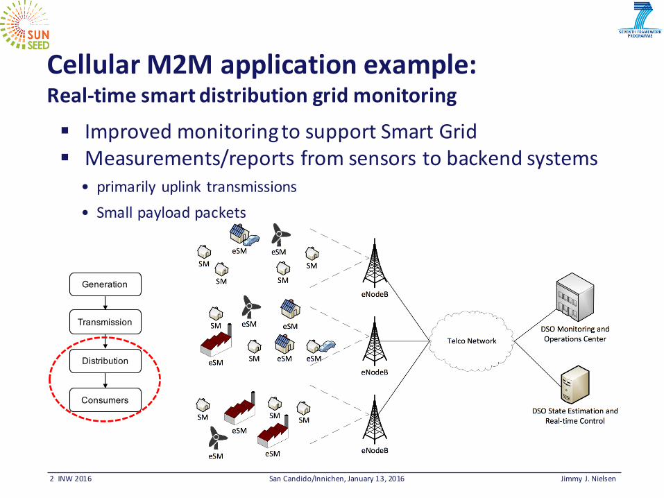
DetailedDescriptionofLTEAccess(1)Downlink(FDDcase):§ 10subframes perframe§ 1subframe is1ms§ Eachsubframehas:
• 14OFDMsymbols intime• 6– 100RBs(depending onBW)(1.4– 20MHz)
§ ForM2MwithoutMIMO:• In1.4MHzsystem:max3PDCCHmessagespersubframe.(thisbottleneckwasusedinGlobecom paper)
• PDSCHcarriesdownlinkARP+signaling messages.
• Limitedresources;formassiveaccess,resourcesmaybescarce.
OFDM Symbols
Resource Block (RB 0)
Resource Block (RB 1)
Resource Block (RB 2)
Resource Block (RB 3)
Resource Block (RB 4)
Resource Block (RB 5)
Frequency
PDCCHPhysical Downlink Control Channel
SSSSecondary Synchronization Signal
PSSPrimary Synchronization Signal
PBCHPhysical Broadcast Channel
PDSCHPhysical Downlink Shared Channel
Slot 0 Slot 1Downlink Subframe 0
PCFICHPhysical Control Format Indicator
Channel
PHICHPhysical Hybrid ARQ Channel
6 INW2016 SanCandido/Innichen,January13,2016 Jimmy J.Nielsen
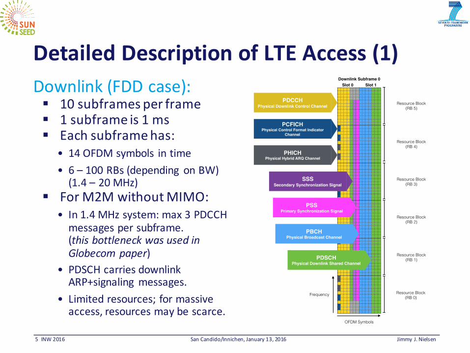
DetailedDescriptionofLTEAccess(2)Uplink:§ PUCCHcanbesharedbymultiple
devices,i.e.notabottleneck.§ Whenpresent,PRACH(RAO)
occupies6RBsperiodically:• 1RAOper20subframes upto1RAOin
everysubframe.§ PUSCHisusedforcontroland
data.• Forlargepayload,itmaybealimiting
factor.
OFDM Symbols
Slot 0 Slot 1
PUCCH (x=0)Physical Uplink Control Channel
PUCCH (x=1)Physical Uplink Control Channel
Slot 0 Slot 1
PRACHPhysical Random Access Channel
Uplink Subframe 0 Uplink Subframe 1
PUSCHPhysical Uplink Shared Channel
Resource Block (RB 0)
Resource Block (RB 1)
Resource Block (RB 2)
Resource Block (RB 3)
Resource Block (RB 4)
Resource Block (RB 5)
RAO: Random Access Opportunity

7 INW2016 SanCandido/Innichen,January13,2016 Jimmy J.Nielsen
DetailedstudyofARPandsignaling
Messageoverview:
5
TABLE IVLIST OF MESSAGES EXCHANGED BETWEEN THE SMART METER AND THE ENODEB.
Step Channel Message
MAC Size (Bytes)
Uplink Downlink
AR
P
1 " PRACH MSG 1: Preamble – –2 # PDCCH Downlink Grant – –3 # PDSCH MSG 2: Random Access Response – 84 " PUSCH MSG 3: RRC Connection Request 7 –
5 # PHICH ACK – –6 # PDCCH Downlink Grant – –7 # PDSCH MSG 4: RRC Connection Setup – 388 # PUCCH ACK – –
Add
ition
alSi
gnal
ing
9 # PUCCH Scheduling Request – –10 # PDCCH UL Grant – –11 # PUSCH RRC Connection Setup Complete (+NAS: Service Req. and Buffer Status) 20 –12 # PHICH ACK – –13 # PDCCH Downlink Grant – –14 # PDSCH Security Mode Command – 1115 " PUCCH ACK – –19 " PUCCH Scheduling Request – –20 # PDCCH UL Grant – –21 " PUSCH Security Mode Complete 13 –22 # PHICH ACK – –16 # PDCCH Downlink Grant – –17 # PDSCH RRC Connection Reconfiguration (+NAS: Activate EPS Bearer Context Req.) – 11818 " PUCCH ACK – –23 " PUCCH Scheduling Request – –24 # PDCCH UL Grant – –25 " PUSCH RRC Connection Reconfiguration Complete 10 –26 # PHICH ACK – –
Dat
a
27 " PUCCH Scheduling Request – –28 # PDCCH UL Grant – –29 " PUSCH Report (Data) Variable –
30 # PHICH ACK – –31 # PDCCH Downlink Grant – –32 # PDSCH RRC Connection Release – 10
Due to the sporadic, i.e., intermittent nature of M2M com-munications, it is typically assumed that the M2M deviceswill have to establish the connection to the cellular accessnetwork every time they perform reporting. From Section IIit becomes apparent that connection establishment requiresextensive signaling, both in the uplink and the downlink, andthe total amount of the signaling information that is exchangedmay well over outweigh the information contained in the datareport. Moreover, the total number of resources available in theuplink and downlink is limited, and in the case of a massivenumber of M2M devices, the signaling traffic related to theestablishment of many connections may pose a significantburden to the operation of the access protocol. Thus, it isof paramount importance to consider the whole procedureassociated with the transmission of a data (report) in orderto properly estimate the number of M2M devices that can besupported in the LTE access network.
A. Related Work
Simple models to determine the probability of preamblecollision (MSG 1) in the PRACH channel are presented in3GPP standard documents [18], [19], [20] and in the scientificliterature [21], [22], [23]. Reception of a preamble is basedon energy detection [24] and a detected preamble indicatesthat there is at least one active user that sends that preamble.The drawback is the inability of the receiver to discern ifa preamble has been selected just by a single device or bymultiple devices [14]. More specifically, the eNodeB can onlyinfer whether the preamble is activated, but not how manydevices have simultaneously activated it.
To alleviate the PRACH overload, a group paging is pro-posed [25], where the base station adjusts the group size toprevent preamble collisions and PDCCH limitation. A relatedanalytical model to represent the number of contending, failed,and success uplink attempts was developed, however, the effectof PDCCH resource limitation has not been taken into account.An investigation of the ARP performance considering theeffect of the limitation of PDCCH resources, by modeling

8 INW2016 SanCandido/Innichen,January13,2016 Jimmy J.Nielsen
LTEAccessReservationModelAccurateanalyticalmodelofserviceoutageprobability• rapidimplementationandevaluation– twoparts:1. One-shottransmission(a)§ Collisionprobability§ ProbabilityofLTEchannelbottlenecklimitations
2. Fullretransmissionmodel(b)§ Failedtransmissionattemptsareretrieduptom=9times.
IdlePopulation
Backlogged
PRACH Data Phase
λI Access Granting
(a)
(b)
λT
λR
NTx< TYes
No
λA
Failure
Success
9 INW2016 SanCandido/Innichen,January13,2016 Jimmy J.Nielsen
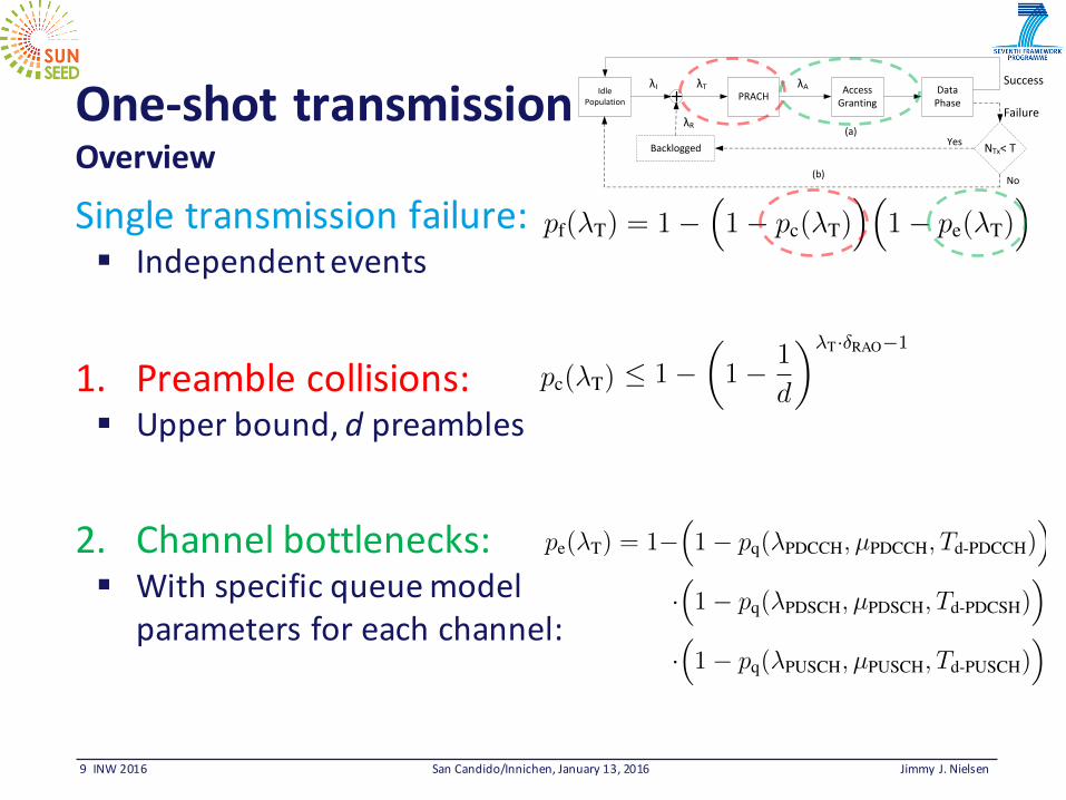
One-shottransmissionOverview
Singletransmissionfailure:§ Independentevents
1. Preamblecollisions:§ Upperbound,d preambles
2. Channelbottlenecks:§ Withspecificqueuemodel
parametersforeachchannel:
13
PUSCH for the required messages. We model this as a sequence of two independent events:
pf(�T) = 1�⇣1� pc(�T)
⌘⇣1� pe(�T)
⌘, (1)
where pf(�T) is the probability of a failed UE transmission, pc(�T) is the collision probability in
the preamble contention phase given UE request rate �T, and pe(�T) is the probability of failure
due to starvation of resources in the PDCCH, PDSCH, or PUSCH.
1) Preamble Contention Phase: We start by computing pc(�T). Let d denote the number of
available preambles (d = 54). Let the probability of not selecting the same preamble as one
other UE be 1� 1d
. Then the probability of a UE selecting a preamble that has been selected by
at least one other UE given at NT contending UEs, is:
P (Collision|NT) = 1�✓1� 1
d
◆NT�1
. (2)
Assuming Poisson arrivals with rate �T, then:
pc(�T) =+1X
i=1
"1�
✓1� 1
d
◆i�1
· P(NT= i,�T · �RAO)
#(3)
1�✓1� 1
d
◆�T·�RAO�1
,
where P(NT = i,�T · �RAO) is the probability mass function of the Poisson distribution with
arrival rate �T · �RAO. The inequality comes from applying Jensen’s inequality to the concave
function 1� (1� 1/d)x, where �T is the total arrival rate (including retransmissions), and �RAO
is the average number of subframes between RAOs.6 The computed pc(�T) is thus an upper
bound on the collision probability.
2) Access Granting Phase: The mean number of activated preambles in the contention phase
per RAO, is given by �A. As discussed in Section III, we assume that the eNodeB is unable
to discern between preambles that have been activated by a single user and multiple users,
respectively. This will lead to a higher �A, than in the case where the eNodeB is able to detect
the preamble collisions. The main impact of this assumption is that there will be an increased
rate of AG requests, even though part of these correspond to collided preambles, which even if
accepted will lead to retransmissions. In addition to the rate of activated preambles �A, we also
need the rate of singletons, i.e., non-collided, successful preamble activations denoted by �S.
6E.g., �RAO =1 if 10 RAOs per frame and �RAO =5 if 2 RAOs per frame.
IdlePopulation
Backlogged
PRACH Data Phase
λI Access Granting
(a)
(b)
λT
λR
NTx< TYes
No
λA
Failure
Success
15
TABLE IVAMOUNT OF CHANNEL RESOURCES USED FOR PDCCH, PDSCH AND PUSCH CHANNELS. FOR SHORT MESSAGE FORMAT,
ONLY BOLD MESSAGES ARE USED (RAR, RRC REQ., RRC COMP., AND DATA).
ARP Additional signaling
RAR
RRC
Request
RRCConnect
RRC
Complete
Reconf.DL
Reconf.UL
SecurityCmd.
SecurityConfig.
SecurityComplete
Data
Channel
PDCCH 1�e��T�RAO�RAO
0 �S �S �S �S �S �S 0 d BdataNfragBRB
ePDSCH d�A
BRARBRB
e 0 �SdBconnBRB
e 0 �SdBr-DLBRB
e 0 �SdBs-cmdBRB
e 0 0 0PUSCH 0 �AdBreq
BRBe 0 �SdBcomp
BRBe 0 �SdBr-UL
BRBe 0 0 �SdBcomp
BRBe �SdBdata
BRBe
PDCCH, PDSCH, and PUSCH, we define pe(�T) from (1) as:
pe(�T) = 1�⇣1� pq(�PDCCH, µPDCCH, Td-PDCCH)
⌘
·⇣1� pq(�PDSCH, µPDSCH, Td-PDCSH)
⌘
·⇣1� pq(�PUSCH, µPUSCH, Td-PUSCH)
⌘, (8)
where the respective �, µ, and Td values are derived in the following. For the � values, we
elaborate in Table IV the amount of resources used in each of the channels for the relevant
messages from Table III. For each, the resources are given in terms of PDCCH, PDSCH, or
PUSCH elements per subframe. The model parameters are described in Table V.
The used M/M/1 model requires a single timeout value to specify the impatience threshold of
the costumers. However, in the modeled LTE access procedure, there are several timers involved
that cover different and sometimes overlapping parts of the message exchange. While this clearly
cannot be modeled very accurately with the used M/M/1 model, we will simply use a typical
minimum timer value for each of the channels. Assuming that LTE has not been designed with
timer values so low that the capacity is limited by timeouts and not by resource scarcity, this
simplifying assumption should not have any significant impact on the results.
a) PDCCH model: The arrival rate for the PDCCH model �PDCCH, which describes the
number of used PDCCH elements per subframe, is given as the sum of the PDCCH row in
Table IV. The service rate µPDCCH is the number of available PDCCH slots per subframe, i.e.,
NPDCCH, and the timer value is the standard RAR timeout:
�PDCCH =1� e��T·�RAO
�RAO+�S(6 + d Bdata
NfragBRBe)
µPDCCH = NPDCCH
10 INW2016 SanCandido/Innichen,January13,2016 Jimmy J.Nielsen
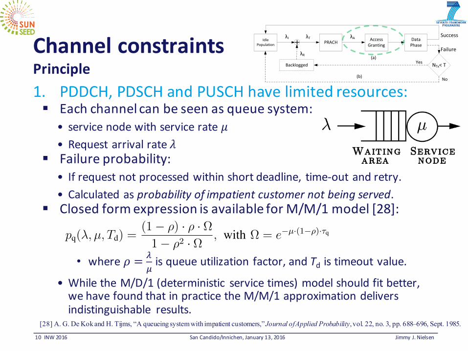
ChannelconstraintsPrinciple1. PDDCH,PDSCHandPUSCHhavelimitedresources:§ Eachchannelcanbeseenasqueuesystem:
• servicenodewithservicerate𝜇• Requestarrivalrate𝜆
§ Failureprobability:• Ifrequestnotprocessedwithinshortdeadline,time-outandretry.• Calculatedasprobabilityofimpatientcustomernotbeingserved.
§ ClosedformexpressionisavailableforM/M/1model[28]:
• where𝜌 = %&isqueue utilization factor,andTd istimeoutvalue.
• WhiletheM/D/1(deterministic servicetimes)modelshouldfitbetter,wehavefoundthatinpracticetheM/M/1approximationdeliversindistinguishable results.
IdlePopulation
Backlogged
PRACH Data Phase
λI Access Granting
(a)
(b)
λT
λR
NTx< TYes
No
λA
Failure
Success
14
The �A and �S can be well approximated, while assuming that the selection of each preamble
by the contending users is independent, by,
�A = [1� P (X = 0)� P (X = 1)] · d/�RAO, (4)
�S =P (X = 1) · d/�RAO, (5)
where P(X = k) is the probability of k successes, which can be well approximated with a
Poisson distribution with arrival rate �pre = �T�RAO/d, i.e.:
P (X = k) ⇡ (�pre)ke��pre
k!. (6)
Since the limitations in the AG phase are primarily given from the demanded resources from
each of the channels PDCCH, PDSCH, and PUSCH and the corresponding timing requirements,
we assume that each of these can be modeled as a separate queue with impatient costumers. That
is, we assume that the loss probability pq(�A) can be seen as the long-run fraction of costumers
that are lost in a queuing system with impatient costumers [26].
Based on the message exchange diagram in Section III-C, we specify in the following text the
arrival rate, service rate and the maximum latency for each of the channels PDCCH, PDSCH,
and PUSCH.
In general, since LTE uses fixed size time slots, the most obvious approach would be to use
an M/D/1 model structure, as presented in [26]. Unfortunately, the expression to compute the
fraction of lost customers pq(�, µ, Td) for the M/D/1 queue does not have a closed form solution.
However the equivalent expression for the M/M/1 queue has a closed form solution. Through an
extensive study, we have found that with the parameter ranges that we use, there is no noticeable
difference in the results. Thus, in the following we use the M/M/1 model to compute pq(�, µ, Td)
as:
pq(�, µ, Td) =(1� ⇢) · ⇢ · ⌦1� ⇢2 · ⌦ , with ⌦ = e�µ·(1�⇢)·⌧q , (7)
where ⇢ = �
µ
is the queue load, µ is the service rate, with ⌧q = Td � 1µ
and Td is the max waiting
time.
Assuming we can use the M/M/1 model structure to obtain the failure probabilities of the[28] A. G. De Kok and H. Tijms, “A queueing system with impatient customers,” Journal of Applied Probability, vol. 22, no. 3, pp. 688–696, Sept. 1985.
11 INW2016 SanCandido/Innichen,January13,2016 Jimmy J.Nielsen
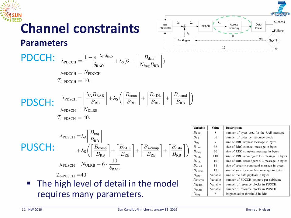
ChannelconstraintsParametersPDCCH:
PDSCH:
PUSCH:
§ Thehighlevelofdetailinthemodelrequiresmanyparameters.
IdlePopulation
Backlogged
PRACH Data Phase
λI Access Granting
(a)
(b)
λT
λR
NTx< TYes
No
λA
Failure
Success
8
where P(X = k) is the probability of k successes, which canbe well approximated with a Poisson distribution with arrivalrate �pre = �T�RAO/d, i.e.:
P (X = k) ⇡(�pre)ke��pre
k!. (6)
Since the limitations in the AG phase are primarily givenfrom the demanded resources from each of the channelsPDCCH, PDSCH, and PUSCH and the corresponding timingrequirements, we assume that each of these can be modeled asa separate queue with impatient costumers. That is, we assumethat the loss probability pq(�A) can be seen as the long-runfraction of costumers that are lost in a queuing system withimpatient costumers [33].
Based on the message exchange diagram in Section II-C,we specify in the following text the arrival rate, service rateand the maximum latency for each of the channels PDCCH,PDSCH, and PUSCH.
In general, since LTE uses fixed size time slots, the mostobvious approach would be to use an M/D/1 model structurewhere service times are deterministic, as presented in [33].Unfortunately, the expression to compute the fraction of lostcustomers pq(�, µ, Td) for the M/D/1 queue does not havea closed form solution. However, the equivalent expressionfor the M/M/1 queue, which assumes exponential durationservice intervals, does have a closed form solution. Throughan extensive study, we have found that with the parameterranges that we use, there is no noticeable difference in theresults. Furthermore, and most importantly, our results withthis model fit well to simulation results, as shown in sec. V-B.Thus, in the following we use the M/M/1 model to computepq(�, µ, Td) as:
pq(�, µ, Td) =(1� ⇢) · ⇢ · ⌦1� ⇢
2 · ⌦ , with ⌦ = e
�µ·(1�⇢)·⌧q, (7)
where ⇢ = �
µ
is the queue load, µ is the service rate, with⌧q = Td � 1
µ
and Td is the max waiting time.Assuming we can use the M/M/1 model structure to obtain
the failure probabilities of the PDCCH, PDSCH, and PUSCH,we define pe(�T) from (1) as:
pe(�T) = 1�⇣1� pq(�PDCCH, µPDCCH, Td-PDCCH)
⌘
·⇣1� pq(�PDSCH, µPDSCH, Td-PDCSH)
⌘
·⇣1� pq(�PUSCH, µPUSCH, Td-PUSCH)
⌘, (8)
where the respective �, µ, and Td values are derived in thefollowing. For the � values, we elaborate in Table VI theamount of resources used in each of the channels for therelevant messages from Table IV. For each, the resources aregiven in terms of PDCCH, PDSCH, or PUSCH elements persubframe. The model parameters are described in Table VII.
The used M/M/1 model requires a single timeout value tospecify the impatience threshold of the costumers. However,in the modeled LTE access procedure, there are several timersinvolved that cover different and sometimes overlapping partsof the message exchange. While this clearly cannot be modeledvery accurately with the M/M/1 model used here, we will
simply use a typical minimum timer value for each of thechannels. Assuming that LTE has not been designed with timervalues so low that the capacity is limited by timeouts and notby resource scarcity, this simplifying assumption should nothave any significant impact on the results.
a) PDCCH model: The arrival rate for the PDCCHmodel �PDCCH, which describes the number of used PDCCHelements per subframe, is given as the sum of the PDCCHrow in Table VI. The service rate µPDCCH is the number ofavailable PDCCH slots per subframe, i.e., NPDCCH, and thetimer value is the standard RAR timeout:
�PDCCH =1� e
��T·�RAO
�RAO+�S(6 +
⇠Bdata
NfragBRB
⇡)
µPDCCH = NPDCCH
Td-PDCCH = 10,
where dxe is the smallest integer not less than x.b) PDSCH model: Similarly, the arrival rate for the
PDSCH model is the sum of the corresponding row in Ta-ble VI, the service rate is the number of available PDSCHelements per subframe, and the timer value is set to 40, whichis a typical minimum value of the PDSCH related timers.
�PDSCH=
⇠�ABRAR
BRB
⇡+�S
✓⇠Bconn
BRB
⇡+
⇠Br-DL
BRB
⇡+
⇠Bs-cmd
BRB
⇡◆
µPDSCH = NDLRB
Td-PDSCH = 40.
c) PUSCH model: Finally, as above, the arrival rate forthe PUSCH model is the sum of the corresponding row inTable VI, the service rate is the number of available PUSCHelements per subframe subtracted the resources used for RAOs,and the timer value is set to 40, which is a typical minimumvalue of the PUSCH related timers.
�PUSCH =�A
⇠Breq
BRB
⇡
+�S
✓⇠Bcomp
BRB
⇡+
⇠Br-UL
BRB
⇡+
⇠Bs-comp
BRB
⇡+
⇠Bdata
BRB
⇡◆
µPUSCH =NULRB � 6 · 10
�RAO
Td-PUSCH =40.
B. m-Retransmissions Model
During the ARP, UEs may experience failures of the trans-mitted packets (MSG1 and MSG3) and the received packets(MSG2 and MSG4). When a failure occurs with probabilitypf(�T), the total arrival rate �T changes to represent also theadditional arrivals of retransmissions. Further, these additionalarrivals affect the probability of failure again. To modelthis behavior, we apply the two-dimensional Markov chainapproach first presented in [34]. The LTE adapted version ofthis model have already been proposed in [31], [35] and in thiswork we consider an extended version of the model in [31] toexplicitly model the transmissions of MSG1 and MSG3.
9
TABLE VIAMOUNT OF CHANNEL RESOURCES USED FOR PDCCH, PDSCH AND PUSCH CHANNELS. FOR SHORT MESSAGE FORMAT, ONLY BOLD MESSAGES ARE
USED (RAR, RRC REQ., RRC COMP., AND DATA).
ARP Additional signaling
Channel RAR
RRC
Request
RRCConnect
RRC
Complete
Reconf.DL
Reconf.UL
SecurityCmd.
SecurityConfig.
SecurityComplete
Data
PDCCH 1�e��T�RAO�RAO
0 �S �S �S �S �S �S 0 d BdataNfragBRB
ePDSCH d�A
BRARBRB
e 0 �SdBconnBRB
e 0 �SdBr-DLBRB
e 0 �SdBs-cmdBRB
e 0 0 0
PUSCH 0 �AdBreqBRB
e 0 �SdBcompBRB
e 0 �SdBr-ULBRB
e 0 0 �SdBcompBRB
e �SdBdataBRB
e
1, 0 1, 1 1, 2 1,𝑊𝑐 − 2 1,𝑊𝑐 − 1"
𝑚, 0 𝑚, 1 𝑚, 2 𝑚,𝑊𝑐 − 2 𝑚,𝑊𝑐 − 1"
𝑖 − 1, 0
𝑖, 0 𝑖, 1 𝑖, 2 𝑖,𝑊𝑐 − 2 𝑖,𝑊𝑐 − 1""/c cp W
"/c cp W
"/c cp W
"/c cp W
"
"
" /c cp W0, 0
1 cp−
𝐶𝑅 1
1 ep−
ep
Connect
𝐶𝑅 𝑖 − 1
𝐶𝑅 𝑖
𝐶𝑅 𝑚
off on1 p−onp𝐶𝑅 0
1 cp−
1 cp−
1 cp−
1 cp−
/e cp W
/e cp W
/e cp W
/e cp W
/e cp W
drop
cp
1
Fig. 6. Markov chain model for m retransmissions during the ARP.
TABLE VIIVARIABLE DEFINITIONS
Variable Value Description
BRAR 8 number of bytes used for the RAR messageBRB 36 number of bytes per resource blockBreq 7 size of RRC request message in bytesBconn 38 size of RRC connect message in bytesBcomp 20 size of RRC complete message in bytesBr-DL 118 size of RRC reconfigure DL message in bytesBr-UL 10 size of RRC reconfigure UL message in bytesBs-cmd 11 size of security command message in bytesBs-comp 13 size of security complete message in bytesBdata Variable size of the data payload in bytesNPDCCH Variable number of PDCCH pointers per subframeNDLRB Variable number of resource blocks in PDSCHNULRB Variable number of resource blocks in PUSCHNfrag 6 fragmentation threshold in RBs
Fig. 6 shows the structure of the Markov chain model form retransmissions during the ARP. The uplink traffic at UEis generated with probability pon. The UE enters the initial
transmission state {0, 0} from the off state:
P (0, 0| off) = pon,
where pon is the traffic generation probability defined as pon =1� e
��I .
The state depicted {i, k} represents the ith preamble re-transmission attempt and kth backoff counter. Retransmissionattempts are allowed up to m times. The maximum backoffwindow size is denoted by W
c
. If a preamble transmission isnot successful, the backoff counter is increased and a randombackoff state is entered with probability:
P ( i, k| i� 1, 0) =p
c
W
c
, 0 k W
c
� 1, 1 i m,
where p
c
denotes the collision probability of the preambletransmission.
The CR(i) state represents the connect request attempt afterthe success of the ith preamble transmission attempt. Thetransition probability is:
P (CR(i)| i, 0) = 1� p
c
, 0 i m.
If the connect request attempt succeeds, the UE will be in

12 INW2016 SanCandido/Innichen,January13,2016 Jimmy J.Nielsen
m-retransmissions§ Fromsteadystateprobabilitiesb*:
§ Iterativeupdatingoffixedpointequationtofind𝜆':
21
Using (18), the value of �T can be obtained by solving the following iterative equation:
�T = NTX(�T) · �I = �I1� (p
e
(1� pc
) + pc
)m+1
1� (pe
(1� pc
) + pc
), (19)
where �I is constant but pc and pe are both functions of �T as defined in (3) and (8).
V. SYSTEM PERFORMANCE EVALUATION
In this section we first describe the used traffic models. Thereafter we present and discuss
numerical results, where we compare results from our analytical model to the simulation results.
A. Model of the Smart Grid Traffic
At the time of writing, there is no standardized traffic model that could be used to describe
reporting activities of the eSMs. In the following, we develop a model by considering the typical
smart metering traffic models and enhancing them in order to achieve PMU-like functionalities
that eSMs are expected to have.
In the literature there are different examples of traffic models for smart meters, such as [29],
[30], [31], [32]. Of these, the OpenSG Smart Grid Networks System Requirements Specification
(described in [29]) from the Utilities Communications Architecture (UCA) user group is the
most coherent and detailed network requirement specification. This specification describes the
typical configuration where billing reports are collected as often as every 1 hour for industrial
smart meters and every 4 hours for residential smart meters. While this is sufficient for billing
purposes, such low reporting frequency does not allow real-time monitoring and control. A way
to enable this, as proposed and analysed in our work in [16], would be to drastically increase
the reporting frequency of all smart meters so that reports are collected, e.g., every 10 seconds.
While such a configuration is not described in OpenSG [29], it is mentioned that on-demand
meter read response messages are 100 bytes, wherefore we will use this value in the following
evaluation.
Besides the basic measurements of consumption and production, the distribution system op-
erators need to collect more detailed information of the distribution grid behavior in the form
of power phasors from certain, strategically chosen, measurement points. As an example in the
following numerical results, we assume that every 10 seconds an eSM sends a measurement
report that consist of concatenated PMU measurements (1 Hz sample rate) from the preceding
10 second measurement interval. The samples are, as specified in PMU standards IEEE 1588 and
!
!
!
!
f/ cp W
!
f/ cp W
!
f/ cp W
!
f/ cp W
!
!
!
f/ cp W
f1 p−
Connect offon
1 p−onp
drop
fp
1
Fig. 3. Markov Chain backoff model to estimate number of requiredtransmissions. The states in the red dashed box are used to calculate NTX.
B. m-Retransmissions Model
When UEs are allowed to make retransmissions the proba-bility of an UE becoming in outage is the probability that noneof the allowed m+1 transmissions attempts are successful.
When retransmissions are allowed (m > 0), the total arrivalrate �T must include the extra arrivals caused by the UEs’retransmissions. The number of retransmissions �R is howevera result of the limit m and transmission error probabilitypf, which in turn depends on the number of retransmissions�R. This chicken and egg problem can be solved iterativelyusing a derivative of the Bianchi model [16] applied to oursystem model. Specifically, we are using a model adapted toLTE, with a structure similar to the one presented in [17].The following derivations of the number of transmissions andoutage probabilities have, to the best of our knowledge, notbeen presented previously.
The mean number of required transmissions NTX and outageprobability Poutage, are computed with help of the Markovchain model depicted in Fig. 3. In the Markov chain model, thestate index {i, k} denotes the ith transmission attempt stageand kth backoff counter. The number of allowed retransmis-sions is then given by m.
Whenever the one-shot transmission is successful, depictedin Fig. 2(a), the UE enters the connect state:
P (connect| i, 0) = 1� pf, 0 i m.
Where, pf is short for pf(�T). Whenever the one-shot accessfails, the UE increases the backoff counter:
P ( i, k| i� 1, 0) =pf
Wc
,
where 0 k Wc
� 1 and 1 i m.At the last stage of the Markov chain, the UE enters the
drop state if the transmission fails:
P (drop|m, 0) = pf(�T).
The UE enters the off state after the connect or the drop states,with probability:
P (off| drop) = P (off| connect) = 1.
From the off state, the node enters the first transmissionstate {0, 0} with probability pon:
P (0, 0| off) = pon.
where the probability pon is defined as pon = 1� e��I .Let b
i,k
be the steady state probability that a UE is at state{i, k}. Then b
i,k
can be derived as:
bi,k
=Wc�k
Wcpfbi�1,0=
Wc�k
Wcpifb0,0=
Wc�k
Wcpifponboff, (7)
for 1 i m and 0 k Wc � 1.Let bconnect be the steady state probability that a node is at
connect state:
bconnect =mX
i=0
(1� pf) bi,0 =mX
i=0
(1� pf) pi
fponboff
=�1� pm+1
f�ponboff.
By imposing the probability normalization condition, asdetailed in Appendix A, we find boff as:
boff =2 (1� pf)
2 (1� pf) (1 + 2pon) + pon (Wc + 1) pf (1� pmf ).
Since a transmission will eventually either finish success-fully in the connect state or unsuccessfully in the drop state,the outage probability can be computed as:
Poutage =bdrop
bdrop + bconnect= pm+1
f , (8)
where bdrop and bconnect, whose derivations are shown in theAppendix A, can be computed as:
bconnect=2 (1�pf)
�1�pm+1
f�pon
2 (1�pf) (1+2pon)+pon (Wc+1) pf (1�pmf ), (9)
bdrop =2 (1�pf) p
m+1f pon
2 (1�pf) (1+2pon)+pon (Wc+1) pf (1�pmf ). (10)
The number of required transmissions can be estimated fromthe steady state probabilities, keeping in mind that b
i,0/b0,0represents the probability of using i+1 or more transmissionattempts to deliver a packet, and b
m,0/b0,0 is the probabilityof using exactly m+1 transmission attempts:
NTX(�T)=
✓m�1Pi=0
(i+ 1) · (bi,0 � b
i+1,0)
◆+ (m+ 1) · b
m,0
b0,0
=(1�pf)m�1X
i=0
(i+1)pif+(m+1) pmf =1� pm+1
f1� pf
.
(11)
From the number of transmissions, the value of �T can besolved iteratively using the fixed point equation:
�T = NTX(�T) · �I = �I1� pf(�T)m+1
1� pf(�T). (12)
!
!
!
!
f/ cp W
!
f/ cp W
!
f/ cp W
!
f/ cp W
!
!
!
f/ cp W
f1 p−
Connect offon
1 p−onp
drop
fp
1
Fig. 3. Markov Chain backoff model to estimate number of requiredtransmissions. The states in the red dashed box are used to calculate NTX.
B. m-Retransmissions Model
When UEs are allowed to make retransmissions the proba-bility of an UE becoming in outage is the probability that noneof the allowed m+1 transmissions attempts are successful.
When retransmissions are allowed (m > 0), the total arrivalrate �T must include the extra arrivals caused by the UEs’retransmissions. The number of retransmissions �R is howevera result of the limit m and transmission error probabilitypf, which in turn depends on the number of retransmissions�R. This chicken and egg problem can be solved iterativelyusing a derivative of the Bianchi model [16] applied to oursystem model. Specifically, we are using a model adapted toLTE, with a structure similar to the one presented in [17].The following derivations of the number of transmissions andoutage probabilities have, to the best of our knowledge, notbeen presented previously.
The mean number of required transmissions NTX and outageprobability Poutage, are computed with help of the Markovchain model depicted in Fig. 3. In the Markov chain model, thestate index {i, k} denotes the ith transmission attempt stageand kth backoff counter. The number of allowed retransmis-sions is then given by m.
Whenever the one-shot transmission is successful, depictedin Fig. 2(a), the UE enters the connect state:
P (connect| i, 0) = 1� pf, 0 i m.
Where, pf is short for pf(�T). Whenever the one-shot accessfails, the UE increases the backoff counter:
P ( i, k| i� 1, 0) =pf
Wc
,
where 0 k Wc
� 1 and 1 i m.At the last stage of the Markov chain, the UE enters the
drop state if the transmission fails:
P (drop|m, 0) = pf(�T).
The UE enters the off state after the connect or the drop states,with probability:
P (off| drop) = P (off| connect) = 1.
From the off state, the node enters the first transmissionstate {0, 0} with probability pon:
P (0, 0| off) = pon.
where the probability pon is defined as pon = 1� e��I .Let b
i,k
be the steady state probability that a UE is at state{i, k}. Then b
i,k
can be derived as:
bi,k
=Wc�k
Wcpfbi�1,0=
Wc�k
Wcpifb0,0=
Wc�k
Wcpifponboff, (7)
for 1 i m and 0 k Wc � 1.Let bconnect be the steady state probability that a node is at
connect state:
bconnect =mX
i=0
(1� pf) bi,0 =mX
i=0
(1� pf) pi
fponboff
=�1� pm+1
f�ponboff.
By imposing the probability normalization condition, asdetailed in Appendix A, we find boff as:
boff =2 (1� pf)
2 (1� pf) (1 + 2pon) + pon (Wc + 1) pf (1� pmf ).
Since a transmission will eventually either finish success-fully in the connect state or unsuccessfully in the drop state,the outage probability can be computed as:
Poutage =bdrop
bdrop + bconnect= pm+1
f , (8)
where bdrop and bconnect, whose derivations are shown in theAppendix A, can be computed as:
bconnect=2 (1�pf)
�1�pm+1
f�pon
2 (1�pf) (1+2pon)+pon (Wc+1) pf (1�pmf ), (9)
bdrop =2 (1�pf) p
m+1f pon
2 (1�pf) (1+2pon)+pon (Wc+1) pf (1�pmf ). (10)
The number of required transmissions can be estimated fromthe steady state probabilities, keeping in mind that b
i,0/b0,0represents the probability of using i+1 or more transmissionattempts to deliver a packet, and b
m,0/b0,0 is the probabilityof using exactly m+1 transmission attempts:
NTX(�T)=
✓m�1Pi=0
(i+ 1) · (bi,0 � b
i+1,0)
◆+ (m+ 1) · b
m,0
b0,0
=(1�pf)m�1X
i=0
(i+1)pif+(m+1) pmf =1� pm+1
f1� pf
.
(11)
From the number of transmissions, the value of �T can besolved iteratively using the fixed point equation:
�T = NTX(�T) · �I = �I1� pf(�T)m+1
1� pf(�T). (12)
IdlePopulation
Backlogged
PRACH Data Phase
λI Access Granting
(a)
(b)
λT
λR
NTx< TYes
No
λA
Failure
Success
1, 0 1, 1 1, 2 1,𝑊𝑐 − 2 1,𝑊𝑐 − 1"
𝑚, 0 𝑚, 1 𝑚, 2 𝑚,𝑊𝑐 − 2 𝑚,𝑊𝑐 − 1"
𝑖 − 1, 0
𝑖, 0 𝑖, 1 𝑖, 2 𝑖,𝑊𝑐 − 2 𝑖,𝑊𝑐 − 1""/c cp W
"/c cp W
"/c cp W
"/c cp W
"
"
" /c cp W0, 0
1 cp−
𝐶𝑅 1
1 ep−
ep
Connect
𝐶𝑅 𝑖 − 1
𝐶𝑅 𝑖
𝐶𝑅 𝑚
off on1 p−onp𝐶𝑅 0
1 cp−
1 cp−
1 cp−
1 cp−
/e cp W
/e cp W
/e cp W
/e cp W
/e cp W
drop
cp
1
Based on LTE-adapted version of Bianchi’s backoff model, by X. Yang, A. Fapojuwo, and E. Egbogah, “Performance Analysis and Parameter Optimization of Random Access Backoff Algorithm in LTE,” in Proc. of the IEEE Vehicular Technology Conference (VTC Fall 2012), Sept. 2012.
13 INW2016 SanCandido/Innichen,January13,2016 Jimmy J.Nielsen
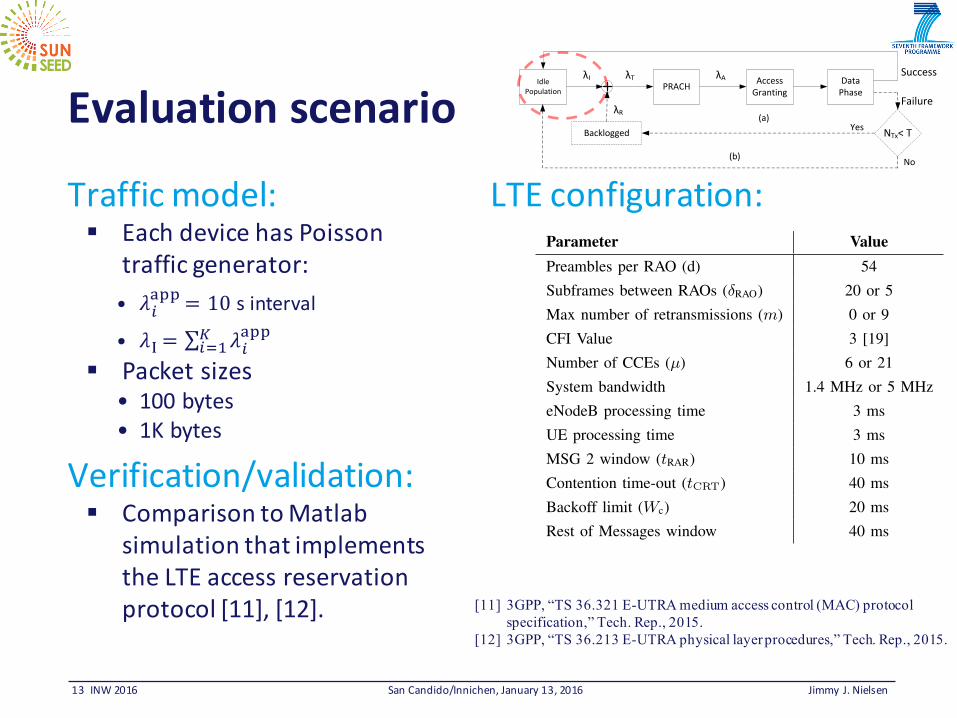
Evaluationscenario
Trafficmodel:§ EachdevicehasPoisson
trafficgenerator:• 𝜆)
*++ = 10 sinterval
• 𝜆. = ∑ 𝜆)*++0
)12§ Packetsizes
• 100bytes• 1Kbytes
Verification/validation:§ ComparisontoMatlab
simulationthatimplementstheLTEaccessreservationprotocol[11],[12].
LTEconfiguration:
IdlePopulation
Backlogged
PRACH Data Phase
λI Access Granting
(a)
(b)
λT
λR
NTx< TYes
No
λA
Failure
Success
[11] 3GPP, “TS 36.321 E-UTRA medium access control (MAC) protocol specification,” Tech. Rep., 2015.
[12] 3GPP, “TS 36.213 E-UTRA physical layer procedures,” Tech. Rep., 2015.
23
TABLE VILTE SIMULATION AND MODEL PARAMETERS
Parameter Value
Preambles per RAO (d) 54Subframes between RAOs (�RAO) 20 or 5Max number of retransmissions (m) 0 or 9CFI Value 3 [19]Number of CCEs (µ) 6 or 21System bandwidth 1.4 MHz or 5 MHzeNodeB processing time 3 msUE processing time 3 msMSG 2 window (tRAR) 10 msContention time-out (tCRT) 40 msBackoff limit (Wc) 20 msRest of Messages window 40 ms
Arrivals/s 0 500 1000 1500 2000 2500 3000 3500 4000
P Out
age
0
0.01
0.02
0.03
0.04
0.05
0.06
0.07
0.08
0.09
0.1Sim: 1.4 MHz - ARP + Data (100 bytes)Ana: 1.4 MHz - ARP + Data (100 bytes)Sim: 1.4 MHz - ARP + Data (1 kbyte)Ana: 1.4 MHz - ARP + Data (1 kbyte)Sim: 5 MHz - ARP + Data (100 bytes)Ana: 5 MHz - ARP + Data (100 bytes)Sim: 5 MHz - ARP + Data (1 kbyte)Ana: 5 MHz - ARP + Data (1 kbyte)
Fig. 7. Probability of outage in LTE with respect the number of M2M arrivals per second in a 1.4 MHz and 5 MHz systemfor different models, payloads and number of RAOs.
transmission starts. That is, we have only the messages shown in bold text in Table IV7. Fig. 7
shows the outage probability Poutage for 1.4 MHz and 5 MHz systems, both for SM and eSM
traffic models. It can be seen that the analytical model is very capable of capturing the outage
7The case where the data transmission occurs immediately after the ARP, without the additional signaling denoted in Table III,is denoted as lightweight-signaling access and corresponds to an extreme case of signaling overhead reduction, beyond whathas been proposed in 3GPP [6], [35].

14 INW2016 SanCandido/Innichen,January13,2016 Jimmy J.Nielsen
Results§ Simulationandmodel
resultsfitclosely.• Both100bytesand1kbytespackets.
§ MAClayer(PUSCH)limitationisclearwhencomparing100bytesto1kbytes:• 1.4MHz:1000à 200arr/s• 5MHz:3900à 800arr/s
Arrivals/s 0 500 1000 1500 2000 2500 3000 3500 4000
P Out
age
0
0.01
0.02
0.03
0.04
0.05
0.06
0.07
0.08
0.09
0.1Sim: 1.4 MHz - ARP + Data (100 bytes)Ana: 1.4 MHz - ARP + Data (100 bytes)Sim: 1.4 MHz - ARP + Data (1 kbyte)Ana: 1.4 MHz - ARP + Data (1 kbyte)Sim: 5 MHz - ARP + Data (100 bytes)Ana: 5 MHz - ARP + Data (100 bytes)Sim: 5 MHz - ARP + Data (1 kbyte)Ana: 5 MHz - ARP + Data (1 kbyte)

15 INW2016 SanCandido/Innichen,January13,2016 Jimmy J.Nielsen
Results§ Simulationandmodel
resultsfitclosely.• Bothwithandwithoutsignaling.
§ Additionalsignalinghaslargeimpactonperformance.• Almosta3xreduction ifomitted!
• LTEforM2Mneedslesssignaling.
4
OFDM Symbols
Slot 0 Slot 1
PUCCH (x=0)Physical Uplink Control Channel
PUCCH (x=1)Physical Uplink Control Channel
Slot 0 Slot 1
PRACHPhysical Random Access Channel
Uplink Subframe 0 Uplink Subframe 1
PUSCHPhysical Uplink Shared Channel
Resource Block (RB 0)
Resource Block (RB 1)
Resource Block (RB 2)
Resource Block (RB 3)
Resource Block (RB 4)
Resource Block (RB 5)
Fig. 3. Simplified illustration of uplink subframe 0 and subframe 1 organi-zation in a 1.4 MHz system with NCFI = 3.
4MSG4 - Contention Resolution
1 MSG1 - Preamble
3 MSG3 - Connection Request
2MSG2 - Random Access Response
eNodeBSmartMeter Additional Signaling (6 messages)
11 Data Transmission
Connection Release 12
Fig. 4. Message exchange between a smart meter and the eNodeB.
d = 54 are typically available for contention purposes andthe rest are reserved for timing alignment. The contention isslotted ALOHA based [11], [12], but unlike in typical ALOHAscenarios, the eNodeB can only detect which preambles havebeen activated but not if multiple activations (collisions) haveoccurred. In particular, this assumption holds in small/urbancells [13, Sec. 17.5.2.3].4
Via MSG 2, the eNodeB returns a random access response(RAR) to all detected preambles. The contending devices listento the downlink channel, expecting MSG 2 within time periodtRAR. If no MSG 2 is received and the maximum of T MSG 1
4If the cell size is more than twice the distance corresponding to themaximum delay spread, the eNodeB may be able to differentiate the casethat preamble has been activated by two or more users, but only if the usersare separable in terms of the Power Delay Profile [13], [14].
transmissions has not been reached, the device backs off andrestarts the random access procedure after a randomly selectedbackoff interval t
r
2 [0,Wc � 1]. If received, MSG 2 includesuplink grant information that indicates the RB in which theconnection request (MSG 3) should be sent. The connectionrequest specifies the requested service type, e.g., voice call,data transmission, measurement report, etc. When two devicesselect the same preamble (MSG 1), they receive the sameMSG 2 and experience collision when they send their MSG 3sin the same RB.
In contrast to the collisions for MSG 1, the eNodeB is ableto detect collisions for MSG 3. The eNodeB only replies to theMSG 3s that did not experience collision, by sending messageMSG 4 (i.e., RRC Connection Setup). The message MSG 4may carry two different outcomes: either the required RBsare allocated or the request is denied in case of insufficientnetwork resources. The latter is however unlikely in the caseof M2M communications, due to the small payloads. If theMSG 4 is not received within time period tCRT since MSG 1was sent, the random access procedure is restarted. Finally,if a device does not successfully finish all the steps of therandom access procedure within m+1 MSG 1 transmissions,an outage is declared.
After ARP exchange finishes, there is an additional ex-change of MAC messages between the smart meter and theeNodeB, whose main purposes is to establish security andquality of service for the connection, as well as to indicatethe status of the buffer at the device. These extra messagesare detailed further in Table IV.
Besides MAC messages, there are PHY messages includedin the connection establishment [15]. Table IV presents acomplete account of both PHY and MAC messages exchangedduring connection establishment, data report transmission andconnection termination (the PHY messages are indicated ingray). As it can be seen from the table, for every downlinkmessage a downlink grant in the PDCCH is required. Simi-larly, every time a smart meter wishes to transmit in the uplinkafter the ARP, it first need to ask for the uplink resourcesby transmitting a scheduling request in the PUCCH.5 This isfollowed by provision of an uplink grant in the PDCCH bythe eNodeB.
III. MOTIVATION, RELATED WORK AND CONTRIBUTIONS
As already outlined, the traffic profile generated by smart-grid monitoring devices is an example of Machine-to-Machine(M2M) traffic, characterized by a sporadic transmissions ofsmall amounts of data from a very large number of terminals.This is in sharp contrast with the bursty and high data-ratetraffic patterns of the human-centered services.
Another important difference is that smart grid servicestypically require a higher degree of network reliability andavailability than the human-centered services [16]. So far,cellular access has been optimized to human-centered trafficand M2M related standardization efforts came into focus onlyrecently [17].
5We note that the amount of resources reserved for PUCCH is very small forscheduling periodicity above 40 ms [15] and therefore will not be consideredin the following text and analysis.
Packet size is 100 bytes
Arrivals/s 0 500 1000 1500 2000 2500 3000 3500 4000
P Out
age
0
0.01
0.02
0.03
0.04
0.05
0.06
0.07
0.08
0.09
0.1
Sim: 1.4 MHz - ARP + DataAna: 1.4 MHz - ARP + DataSim: 1.4 MHz - ARP + Signaling + DataAna: 1.4 MHz - ARP + Signaling + DataSim: 5 MHz - ARP + DataAna: 5 MHz - ARP + DataSim: 5 MHz - ARP + Signaling + DataAna: 5 MHz - ARP + Signaling + Data
Signaling impact
Signaling Impact
16 INW2016 SanCandido/Innichen,January13,2016 Jimmy J.Nielsen
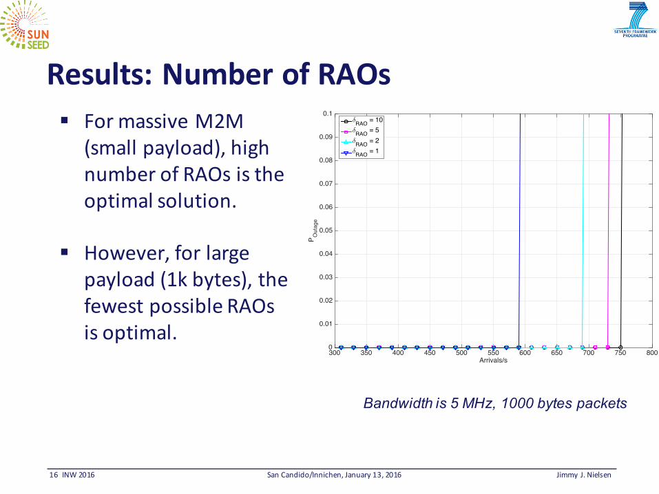
Results:NumberofRAOs§ FormassiveM2M
(smallpayload),highnumberofRAOsistheoptimalsolution.
§ However,forlargepayload(1kbytes),thefewestpossibleRAOsisoptimal.
Arrivals/s 300 350 400 450 500 550 600 650 700 750 800
P Out
age
0
0.01
0.02
0.03
0.04
0.05
0.06
0.07
0.08
0.09
0.1δRAO = 10δRAO = 5δRAO = 2δRAO = 1
Bandwidth is 5 MHz, 1000 bytes packets

17 INW2016 SanCandido/Innichen,January13,2016 Jimmy J.Nielsen
Results:ARPonlyvs PHYandMAC§ 100bytes
• PDCCHlimits(PHY/signaling)
§ 1kbytes• PUSCHlimitsduetodata.
§ ImportanttoaccountforPHYandMAClimitations!
Arrivals/s ×1040 0.5 1 1.5 2 2.5 3 3.5 4
P Out
age
0
0.01
0.02
0.03
0.04
0.05
0.06
0.07
0.08
0.09
0.1100 bytes1 kbyte100 bytes and 1000 bytes (ideal PHY and MAC)
2 RAOs per 10 subframes

18 INW2016 SanCandido/Innichen,January13,2016 Jimmy J.Nielsen
Conclusion
1. Necessarytotakeintoaccountchannellimitations:§ M2M(smallpayload):PRACH andPDCCHlimits.§ Largepayload:PUSCHlimits.
2. Rapidimplementation(comparedtosimulations)andclick-speedevaluationofoutagebreakpoint.
3. SignalingafterARPhasbigimpactonM2Mperformance.
§ Reducedsignalingshouldbeinvestigated.
19 INW2016 SanCandido/Innichen,January13,2016 Jimmy J.Nielsen
Backupslides
20 INW2016 SanCandido/Innichen,January13,2016 Jimmy J.Nielsen
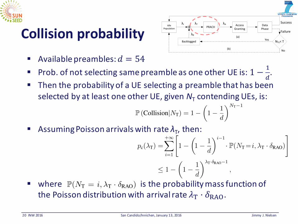
Collisionprobability§ Availablepreambles:𝑑 = 54§ Prob.ofnotselectingsamepreambleasoneotherUEis:1 − 2
7.
§ ThentheprobabilityofaUEselectingapreamblethathasbeenselectedbyatleastoneotherUE,givenNT contendingUEs,is:
§ AssumingPoissonarrivalswithrateλT,then:
§ where istheprobabilitymassfunctionofthePoissondistributionwitharrivalrate𝜆' · 𝛿:;<.
should be sent. The connection request specifies the requestedservice type, e.g., voice call, data transmission, measurementreport, etc. In case of collision the devices receive the sameMSG 2, resulting in their MSG 3s colliding in the RB.
In contrast to the collisions of MSG 1, the eNodeB is ableto detect collisions of MSG 3. The eNodeB only replies tothe MSG 3s that did not experience collision, by sendingmessage MSG 4, with which the required RBs are allocatedor the request is denied in case of insufficient resources.The latter is however unlikely in the case of MTC, due tothe small payloads. If the MSG 4 is not received withintCRT since MSG 1 was sent, the random access procedureis restarted. Finally, if a device does not successfully finish allthe steps of the random access procedure within m+1 MSG 1transmissions, an outage is declared.
III. MODELING THE ACCESS RESERVATION PROTOCOL
We now go to the analysis of the access reservation pro-cedure. First, we model the One-shot transmission and thenextend it to the m-Retransmissions model. The numericalresults cover the complete model, as depicted in Fig. 2.
A. One-Shot Transmission Model
We are interested in characterizing how often a transmissionfrom a UE fails. This happens when the transmission is notsuccessful in both the preamble contention and AG phases,i.e., a request from the UE must not experience a preamblecollision and the uplink grant must not become stale anddropped. We model this as two independent events:
pf(�T) = 1�⇣1� pc(�T)
⌘⇣1� pe(�A)
⌘, (1)
where pc(�T) is the collision probability in the preamblecontention phase given UE request rate �T, while pe(�A) isthe probability of the uplink grant being dropped from the AGqueue given preamble activation rate �A.
1) Preamble Contention Phase: We start by computingpc(�T). Let d denote the number of available preambles(d = 54). Let the probability of not selecting the samepreamble as one other UE be 1 � 1
d
. Then the probability ofa UE selecting a preamble that has been selected by at leastone other UE, given NT contending UEs, is:
P (Collision|NT) = 1�✓1� 1
d
◆NT�1
. (2)
Assuming Poisson arrivals with rate �T, then:
pc(�T) =+1X
i=1
"1�
✓1� 1
d
◆i�1
· P(NT= i,�T · �RAO)
#(3)
1�✓1� 1
d
◆�T·�RAO�1
,
where P(NT = i,�T · �RAO) is the probability mass functionof the Poisson distribution with arrival rate �T · �RAO. Theinequality comes from applying Jensen’s inequality to the con-cave function 1�(1� 1/d)x, where �T is the total arrival rate(including retransmissions), and �RAO is the average number
of subframes between RAOs.2 The computed pc(�T) is thusan upper bound on the collision probability.
2) Access Granting Phase: The mean number of activatedpreambles in the contention phase per RAO, is given by �A. Asdiscussed in Section II, we assume that the eNodeB is unableto discern between preambles that have been activated by asingle user and multiple users, respectively. This will lead to ahigher �A, than in the case where the eNodeB is able to detectthe preamble collisions. The main impact of this assumptionis that there will be an increased rate of AG requests, eventhough part of these correspond to collided preambles, whicheven if accepted will lead to retransmissions.
The �A can be well approximated, while assuming thatthe selection of each preamble by the contending users isindependent, by,
�A = [1� P (X = 0)� P (X = 1)] · d, (4)
where P(X = k) is the probability of k successes, which canbe well approximated with a Poisson distribution with arrivalrate �T/d, i.e.:
P (X = k) ⇡ (�T/d)ke��T/d
k!. (5)
To compute the outage probability due to the limitation inthe AG phase, i.e., due to the maximum number of uplinkgrants per subframe and a maximum waiting time of tRARsubframes, we consider that this subsystem can be modeled asa queuing system. We assume that the loss probability pe(�A)can be seen as the long-run fraction of costumers that are lostin a queuing system with impatient costumers [15].
In LTE, pending uplink grants are served with a determin-istic time interval (1 subframe) between each serving slot [8].A straightforward approach would be to use an M/D/1 modelstructure, as presented in [15], in order to compute the dropprobability. Unfortunately, the expression to compute pe(�A)for the M/D/1 queue does not have a closed-form solution.However the equivalent expression for the M/M/1 queue in[15] has a closed-form solution, see eq. (6). We have comparedthe results of the two model types and found no noticeabledifference in the computed outage numbers in practice. Thus,in the following we use the M/M/1 model to compute pe(�A):
pe(�A) =(1� ⇢) · ⇢ · ⌦1� ⇢2 · ⌦ , with ⌦ = e�µ·(1�⇢)·⌧q . (6)
where ⇢ = �Aµ
is the queue load, µ is the number of uplinkgrants per RAR (µ = 3), with ⌧q = Td � 1
µ
and Td is the maxwaiting time (in terms of requests) in the uplink grant queue,i.e., Td = µ · tRAR.
The fact that we are using an M/M/1 model instead of anM/D/1 model, may cause a discrepancy between the simulationand model results when the queue becomes congested (⇢ > 1).However, we are interested in the switching point (⇢ = 1) fromwhich we then estimate accurately the outage breaking point,as shown in the results in section IV.
2E.g., �RAO =1 if 10 RAOs per frame and �RAO =5 if 2 RAOs per frame.
13
PUSCH for the required messages. We model this as a sequence of two independent events:
pf(�T) = 1�⇣1� pc(�T)
⌘⇣1� pe(�T)
⌘, (1)
where pf(�T) is the probability of a failed UE transmission, pc(�T) is the collision probability in
the preamble contention phase given UE request rate �T, and pe(�T) is the probability of failure
due to starvation of resources in the PDCCH, PDSCH, or PUSCH.
1) Preamble Contention Phase: We start by computing pc(�T). Let d denote the number of
available preambles (d = 54). Let the probability of not selecting the same preamble as one
other UE be 1� 1d
. Then the probability of a UE selecting a preamble that has been selected by
at least one other UE given at NT contending UEs, is:
P (Collision|NT) = 1�✓1� 1
d
◆NT�1
. (2)
Assuming Poisson arrivals with rate �T, then:
pc(�T) =+1X
i=1
"1�
✓1� 1
d
◆i�1
· P(NT= i,�T · �RAO)
#(3)
1�✓1� 1
d
◆�T·�RAO�1
,
where P(NT = i,�T · �RAO) is the probability mass function of the Poisson distribution with
arrival rate �T · �RAO. The inequality comes from applying Jensen’s inequality to the concave
function 1� (1� 1/d)x, where �T is the total arrival rate (including retransmissions), and �RAO
is the average number of subframes between RAOs.6 The computed pc(�T) is thus an upper
bound on the collision probability.
2) Access Granting Phase: The mean number of activated preambles in the contention phase
per RAO, is given by �A. As discussed in Section III, we assume that the eNodeB is unable
to discern between preambles that have been activated by a single user and multiple users,
respectively. This will lead to a higher �A, than in the case where the eNodeB is able to detect
the preamble collisions. The main impact of this assumption is that there will be an increased
rate of AG requests, even though part of these correspond to collided preambles, which even if
accepted will lead to retransmissions. In addition to the rate of activated preambles �A, we also
need the rate of singletons, i.e., non-collided, successful preamble activations denoted by �S.
6E.g., �RAO =1 if 10 RAOs per frame and �RAO =5 if 2 RAOs per frame.
should be sent. The connection request specifies the requestedservice type, e.g., voice call, data transmission, measurementreport, etc. In case of collision the devices receive the sameMSG 2, resulting in their MSG 3s colliding in the RB.
In contrast to the collisions of MSG 1, the eNodeB is ableto detect collisions of MSG 3. The eNodeB only replies tothe MSG 3s that did not experience collision, by sendingmessage MSG 4, with which the required RBs are allocatedor the request is denied in case of insufficient resources.The latter is however unlikely in the case of MTC, due tothe small payloads. If the MSG 4 is not received withintCRT since MSG 1 was sent, the random access procedureis restarted. Finally, if a device does not successfully finish allthe steps of the random access procedure within m+1 MSG 1transmissions, an outage is declared.
III. MODELING THE ACCESS RESERVATION PROTOCOL
We now go to the analysis of the access reservation pro-cedure. First, we model the One-shot transmission and thenextend it to the m-Retransmissions model. The numericalresults cover the complete model, as depicted in Fig. 2.
A. One-Shot Transmission Model
We are interested in characterizing how often a transmissionfrom a UE fails. This happens when the transmission is notsuccessful in both the preamble contention and AG phases,i.e., a request from the UE must not experience a preamblecollision and the uplink grant must not become stale anddropped. We model this as two independent events:
pf(�T) = 1�⇣1� pc(�T)
⌘⇣1� pe(�A)
⌘, (1)
where pc(�T) is the collision probability in the preamblecontention phase given UE request rate �T, while pe(�A) isthe probability of the uplink grant being dropped from the AGqueue given preamble activation rate �A.
1) Preamble Contention Phase: We start by computingpc(�T). Let d denote the number of available preambles(d = 54). Let the probability of not selecting the samepreamble as one other UE be 1 � 1
d
. Then the probability ofa UE selecting a preamble that has been selected by at leastone other UE, given NT contending UEs, is:
P (Collision|NT) = 1�✓1� 1
d
◆NT�1
. (2)
Assuming Poisson arrivals with rate �T, then:
pc(�T) =+1X
i=1
"1�
✓1� 1
d
◆i�1
· P(NT= i,�T · �RAO)
#(3)
1�✓1� 1
d
◆�T·�RAO�1
,
where P(NT = i,�T · �RAO) is the probability mass functionof the Poisson distribution with arrival rate �T · �RAO. Theinequality comes from applying Jensen’s inequality to the con-cave function 1�(1� 1/d)x, where �T is the total arrival rate(including retransmissions), and �RAO is the average number
of subframes between RAOs.2 The computed pc(�T) is thusan upper bound on the collision probability.
2) Access Granting Phase: The mean number of activatedpreambles in the contention phase per RAO, is given by �A. Asdiscussed in Section II, we assume that the eNodeB is unableto discern between preambles that have been activated by asingle user and multiple users, respectively. This will lead to ahigher �A, than in the case where the eNodeB is able to detectthe preamble collisions. The main impact of this assumptionis that there will be an increased rate of AG requests, eventhough part of these correspond to collided preambles, whicheven if accepted will lead to retransmissions.
The �A can be well approximated, while assuming thatthe selection of each preamble by the contending users isindependent, by,
�A = [1� P (X = 0)� P (X = 1)] · d, (4)
where P(X = k) is the probability of k successes, which canbe well approximated with a Poisson distribution with arrivalrate �T/d, i.e.:
P (X = k) ⇡ (�T/d)ke��T/d
k!. (5)
To compute the outage probability due to the limitation inthe AG phase, i.e., due to the maximum number of uplinkgrants per subframe and a maximum waiting time of tRARsubframes, we consider that this subsystem can be modeled asa queuing system. We assume that the loss probability pe(�A)can be seen as the long-run fraction of costumers that are lostin a queuing system with impatient costumers [15].
In LTE, pending uplink grants are served with a determin-istic time interval (1 subframe) between each serving slot [8].A straightforward approach would be to use an M/D/1 modelstructure, as presented in [15], in order to compute the dropprobability. Unfortunately, the expression to compute pe(�A)for the M/D/1 queue does not have a closed-form solution.However the equivalent expression for the M/M/1 queue in[15] has a closed-form solution, see eq. (6). We have comparedthe results of the two model types and found no noticeabledifference in the computed outage numbers in practice. Thus,in the following we use the M/M/1 model to compute pe(�A):
pe(�A) =(1� ⇢) · ⇢ · ⌦1� ⇢2 · ⌦ , with ⌦ = e�µ·(1�⇢)·⌧q . (6)
where ⇢ = �Aµ
is the queue load, µ is the number of uplinkgrants per RAR (µ = 3), with ⌧q = Td � 1
µ
and Td is the maxwaiting time (in terms of requests) in the uplink grant queue,i.e., Td = µ · tRAR.
The fact that we are using an M/M/1 model instead of anM/D/1 model, may cause a discrepancy between the simulationand model results when the queue becomes congested (⇢ > 1).However, we are interested in the switching point (⇢ = 1) fromwhich we then estimate accurately the outage breaking point,as shown in the results in section IV.
2E.g., �RAO =1 if 10 RAOs per frame and �RAO =5 if 2 RAOs per frame.
IdlePopulation
Backlogged
PRACH Data Phase
λI Access Granting
(a)
(b)
λT
λR
NTx< TYes
No
λA
Failure
Success
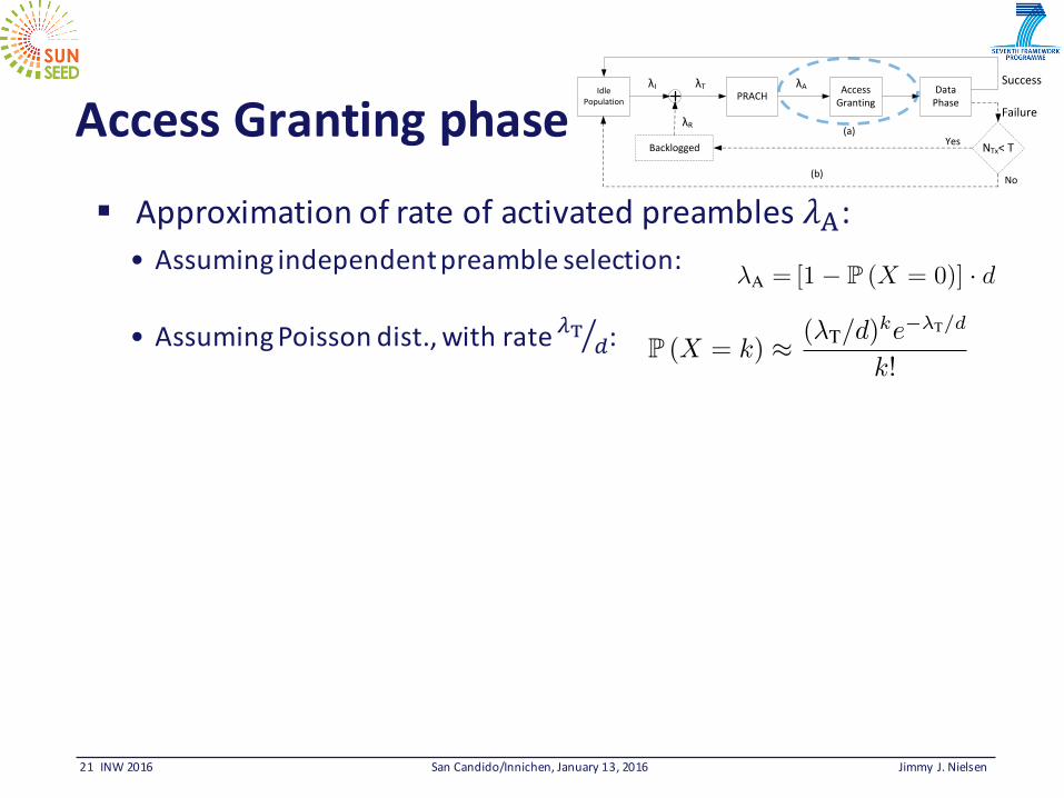
21 INW2016 SanCandido/Innichen,January13,2016 Jimmy J.Nielsen
AccessGrantingphase
§ Approximationofrateofactivatedpreambles𝜆;:• Assumingindependentpreambleselection:
• AssumingPoissondist.,withrate%= 7> :
IdlePopulation
Backlogged
PRACH Data Phase
λI Access Granting
(a)
(b)
λT
λR
NTx< TYes
No
λA
Failure
Success
should be sent. The connection request specifies the requestedservice type, e.g., voice call, data transmission, measurementreport, etc. In case of collision the devices receive the sameMSG 2, resulting in their MSG 3s colliding in the RB.
In contrast to the collisions of MSG 1, the eNodeB is ableto detect collisions of MSG 3. The eNodeB only replies tothe MSG 3s that did not experience collision, by sendingmessage MSG 4, with which the required RBs are allocatedor the request is denied in case of insufficient resources.The latter is however unlikely in the case of MTC, due tothe small payloads. If the MSG 4 is not received withintCRT since MSG 1 was sent, the random access procedureis restarted. Finally, if a device does not successfully finish allthe steps of the random access procedure within m+1 MSG 1transmissions, an outage is declared.
III. MODELING THE ACCESS RESERVATION PROTOCOL
We now go to the analysis of the access reservation pro-cedure. First, we model the One-shot transmission and thenextend it to the m-Retransmissions model. The numericalresults cover the complete model, as depicted in Fig. 2.
A. One-Shot Transmission Model
We are interested in characterizing how often a transmissionfrom a UE fails. This happens when the transmission is notsuccessful in both the preamble contention and AG phases,i.e., a request from the UE must not experience a preamblecollision and the uplink grant must not become stale anddropped. We model this as two independent events:
pf(�T) = 1�⇣1� pc(�T)
⌘⇣1� pe(�A)
⌘, (1)
where pc(�T) is the collision probability in the preamblecontention phase given UE request rate �T, while pe(�A) isthe probability of the uplink grant being dropped from the AGqueue given preamble activation rate �A.
1) Preamble Contention Phase: We start by computingpc(�T). Let d denote the number of available preambles(d = 54). Let the probability of not selecting the samepreamble as one other UE be 1 � 1
d
. Then the probability ofa UE selecting a preamble that has been selected by at leastone other UE, given NT contending UEs, is:
P (Collision|NT) = 1�✓1� 1
d
◆NT�1
. (2)
Assuming Poisson arrivals with rate �T, then:
pc(�T) =+1X
i=1
"1�
✓1� 1
d
◆i�1
· P(NT= i,�T · �RAO)
#(3)
1�✓1� 1
d
◆�T·�RAO�1
,
where P(NT = i,�T · �RAO) is the probability mass functionof the Poisson distribution with arrival rate �T · �RAO. Theinequality comes from applying Jensen’s inequality to the con-cave function 1�(1� 1/d)x, where �T is the total arrival rate(including retransmissions), and �RAO is the average number
of subframes between RAOs.2 The computed pc(�T) is thusan upper bound on the collision probability.
2) Access Granting Phase: The mean number of activatedpreambles in the contention phase per RAO, is given by �A. Asdiscussed in Section II, we assume that the eNodeB is unableto discern between preambles that have been activated by asingle user and multiple users, respectively. This will lead to ahigher �A, than in the case where the eNodeB is able to detectthe preamble collisions. The main impact of this assumptionis that there will be an increased rate of AG requests, eventhough part of these correspond to collided preambles, whicheven if accepted will lead to retransmissions.
The �A can be well approximated, while assuming thatthe selection of each preamble by the contending users isindependent, by,
�A = [1� P (X = 0)� P (X = 1)] · d, (4)
where P(X = k) is the probability of k successes, which canbe well approximated with a Poisson distribution with arrivalrate �T/d, i.e.:
P (X = k) ⇡ (�T/d)ke��T/d
k!. (5)
To compute the outage probability due to the limitation inthe AG phase, i.e., due to the maximum number of uplinkgrants per subframe and a maximum waiting time of tRARsubframes, we consider that this subsystem can be modeled asa queuing system. We assume that the loss probability pe(�A)can be seen as the long-run fraction of costumers that are lostin a queuing system with impatient costumers [15].
In LTE, pending uplink grants are served with a determin-istic time interval (1 subframe) between each serving slot [8].A straightforward approach would be to use an M/D/1 modelstructure, as presented in [15], in order to compute the dropprobability. Unfortunately, the expression to compute pe(�A)for the M/D/1 queue does not have a closed-form solution.However the equivalent expression for the M/M/1 queue in[15] has a closed-form solution, see eq. (6). We have comparedthe results of the two model types and found no noticeabledifference in the computed outage numbers in practice. Thus,in the following we use the M/M/1 model to compute pe(�A):
pe(�A) =(1� ⇢) · ⇢ · ⌦1� ⇢2 · ⌦ , with ⌦ = e�µ·(1�⇢)·⌧q . (6)
where ⇢ = �Aµ
is the queue load, µ is the number of uplinkgrants per RAR (µ = 3), with ⌧q = Td � 1
µ
and Td is the maxwaiting time (in terms of requests) in the uplink grant queue,i.e., Td = µ · tRAR.
The fact that we are using an M/M/1 model instead of anM/D/1 model, may cause a discrepancy between the simulationand model results when the queue becomes congested (⇢ > 1).However, we are interested in the switching point (⇢ = 1) fromwhich we then estimate accurately the outage breaking point,as shown in the results in section IV.
2E.g., �RAO =1 if 10 RAOs per frame and �RAO =5 if 2 RAOs per frame.
15
to discern between preambles that have been activated by a single user and multiple users,
respectively. This will lead to a higher �A, than in the case where the eNodeB is able to detect
the preamble collisions. The main impact of this assumption is that there will be an increased rate
of access granted requests, even though part of these correspond to collided preambles, which
even if accepted will lead to retransmissions. In addition to the rate of activated preambles �A,
we also need the rate of singletons, i.e., non-collided, successful preamble activations denoted
by �S.
The �A and �S can be well approximated, while assuming that the selection of each preamble
by the contending users is independent, by,
�A = [1� P (X = 0)] · d/�RAO, (4)
�S =P (X = 1) · d/�RAO, (5)
where P(X = k) is the probability of k successes, which can be well approximated with a
Poisson distribution with arrival rate �pre = �T�RAO/d, i.e.:
P (X = k) ⇡ (�pre)ke��pre
k!. (6)
Since the limitations in the AG phase are primarily given from the demanded resources from
each of the channels PDCCH, PDSCH, and PUSCH and the corresponding timing requirements,
we assume that each of these can be modeled as a separate queue with impatient costumers. That
is, we assume that the loss probability pq(�A) can be seen as the long-run fraction of costumers
that are lost in a queuing system with impatient costumers [33].
Based on the message exchange diagram in Section II-C, we specify in the following text the
arrival rate, service rate and the maximum latency for each of the channels PDCCH, PDSCH,
and PUSCH.
In general, since LTE uses fixed size time slots, the most obvious approach would be to use an
M/D/1 model structure where service times are deterministic, as presented in [33]. Unfortunately,
the expression to compute the fraction of lost customers pq(�, µ, Td) for the M/D/1 queue does
not have a closed form solution. However, the equivalent expression for the M/M/1 queue, which
assumes exponential duration service intervals, does have a closed form solution. Through an
extensive study, we have found that with the parameter ranges that we use, there is no noticeable
difference in the results. Furthermore, and most importantly, our results with this model fit well


![Tractable Approximate Robust Geometric Programmingweb.stanford.edu/~boyd/papers/pdf/rgp-full.pdf · Tractable Approximate Robust Geometric Programming ... KC97], power control of](https://static.fdocuments.in/doc/165x107/5c9d5fd088c9939c348cafed/tractable-approximate-robust-geometric-boydpaperspdfrgp-fullpdf-tractable.jpg)