A tool for nonlinear dynamic optimization

Arenberg Youngsters Seminar – October 10, 2018

Joris GillisPhD in electrical engineeringPost-doc at mechanical engineering MECO PMA MECH.∈. .∈.

“Everything is an optimization problem”

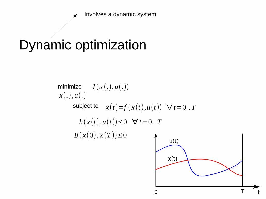
Dynamic optimization

J (x (.), u(.))minimize

x(.) ,u(.)

subject to x(t )=f (x (t ) ,u(t )) ∀ t=0. .T

h(x (t ) ,u(t ))≤0 ∀ t=0. .T

Involves a dynamic system

B(x(0) , x (T ))≤0

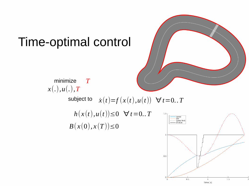
Time-optimal control

Tminimize

x(.) ,u(.) ,Tsubject to x(t )=f (x (t ) ,u(t )) ∀ t=0. .T

h(x (t ) ,u(t ))≤0 ∀ t=0. .T

B(x(0) , x (T ))≤0

Model predictive control (MPC)

J (x (.), u(.))minimize

x(.) ,u(.)

subject to x(t )=f (x (t ) ,u(t )) ∀ t=0. .T

x(0)= x0

h(x (t ) ,u(t ))≤0 ∀ t=0. .T

timeCurrent sample

Predict future controls

Find next control input

Moving horizon estimation (MHE)

∫−T

0‖y (x(t ))− y(t )‖2

2 dtminimizex(.)

subject to x(t )=f (x (t ) , u(t )) ∀ t=−T ..0

h(x (t ) , u(t ))≤0 ∀ t=−T ..0

timeCurrent sample

Fit the measurements

Find current state

u(t ) y (t )Observed outputApplied input

Offline parameter estimation

∫0

T‖y (x (t ))− y (t )‖2

2dtminimize

x(.) , p

subject to x(t )=f (x (t ) , u(t ) , p) ∀ t=0. .T

u(t ) y (t )Observed outputApplied input

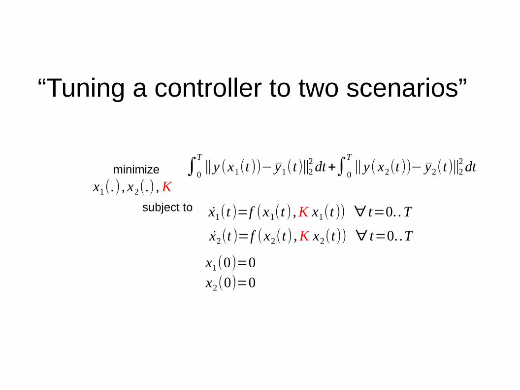
“Tuning a controller to two scenarios”

minimize

x1(.) , x2(.) , Ksubject to

∫0

T‖y (x1(t ))− y1(t)‖2

2 dt+∫0

T‖y(x2(t ))− y2(t)‖2

2 dt

x1(t )=f (x1(t ) , K x1(t )) ∀ t=0. .T

x2(t )=f (x2(t) , K x2(t)) ∀ t=0. .T

x1(0)=0

x2(0)=0

J (x (.), u(.), p)minimize

x(.) ,u(.) , psubject to x(t )=f (x (t ) ,u(t ) , p) ∀ t=0. .T

h (x (t ) ,u(t ))≤0 ∀ t=0. .T

B(x(0) , x (T ))≤0

System design

Especially true in engineeringEspecially true during a PhD

“Everything is a dynamic optimization problem”

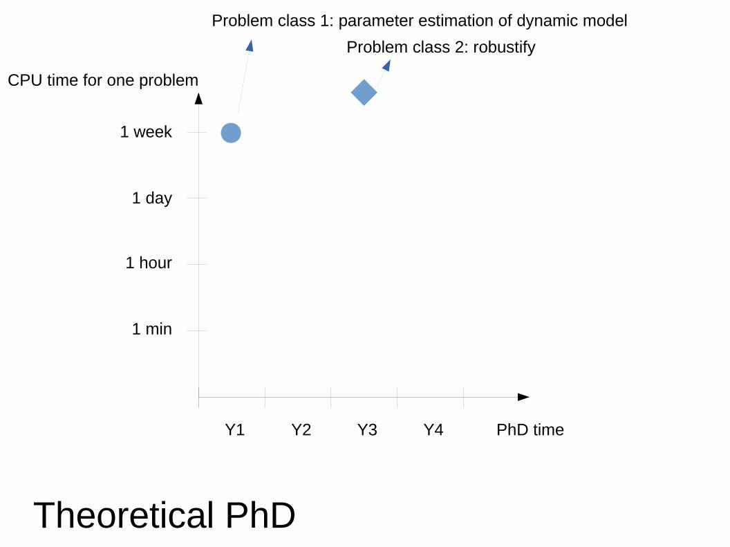
PhD timeY1 Y2 Y3 Y4

1 min

1 hour

1 week

1 day

CPU time for one problem

Problem class 1: parameter estimation of dynamic model

Problem class 2: robustify

Theoretical PhD

PhD timeY1 Y2 Y3 Y4

1 min

1 hour

1 week

1 day

CPU time for one problem

Practical PhD

Choice of solverSparsity exploitationExact derivativesImplementation in CParallelization

PhD timeY1 Y2 Y3 Y4

1 min

1 hour

1 week

1 day

CPU time for one problem

State-of-the-art

Numerical methods PhD

Toy problem

PhD timeY1 Y2 Y3 Y4

1 min

1 hour

1 week

1 day

CPU time for one problem

Universal PhD?

State-of-the-art

Time to work on applications/theory

Use powerful tools to make prototypes very fast

Dig a bit deeper for most interesting problem class

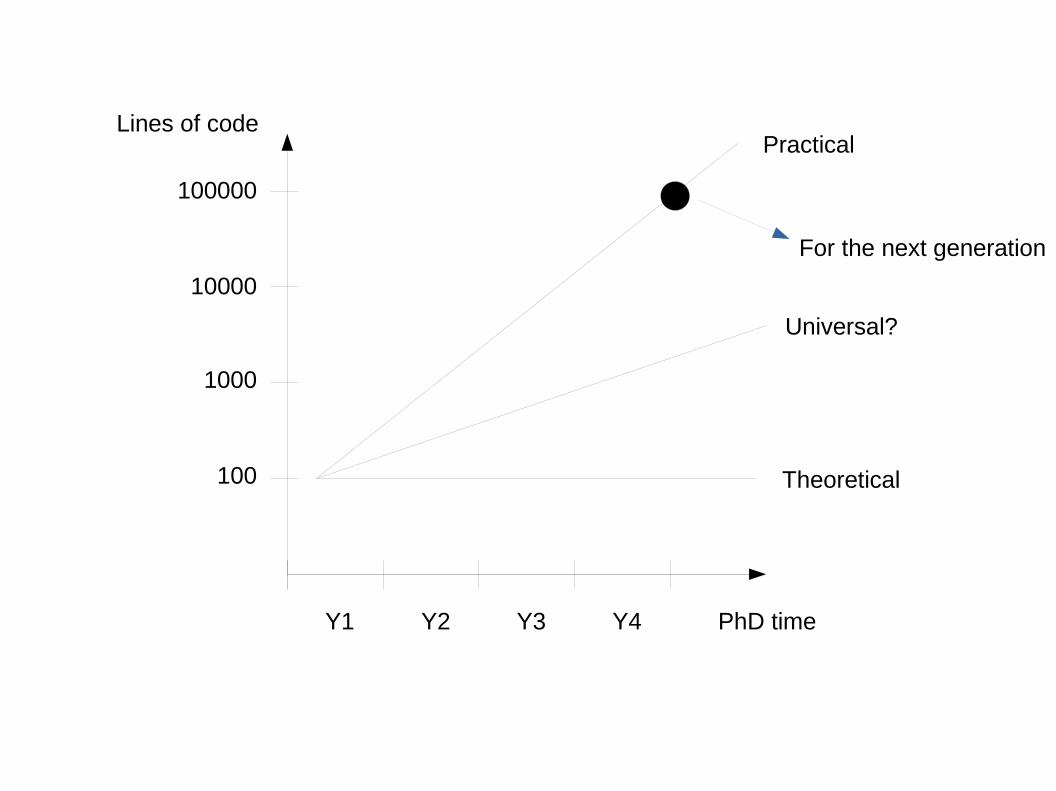
PhD timeY1 Y2 Y3 Y4

100

1000

100000

10000

Lines of code

Theoretical

Practical

Universal?

For the next generation

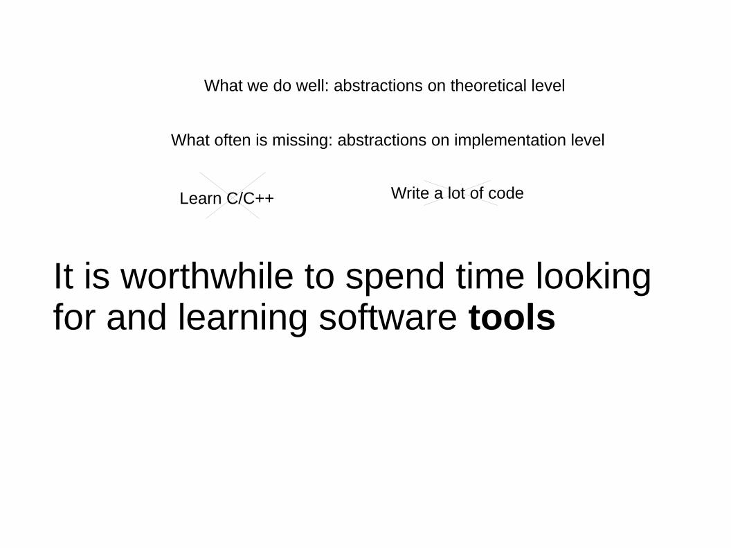
It is worthwhile to spend time looking for and learning software tools

What we do well: abstractions on theoretical level

What often is missing: abstractions on implementation level

Learn C/C++ Write a lot of code

Joel A. E. Andersson, Joris Gillis, Greg Horn, James B. Rawlings, Moritz Diehl,

“CasADi – A software framework for nonlinear optimization and optimal control,”

Mathematical Programming Computation, 2018.

Some application areas:

● Iceberg monitoring

● Bio-reactors

● Thermal control of buildings

● Wind energy

http://casadi.org Workshop http://leuven2018.casadi.org

Continuous decision variables

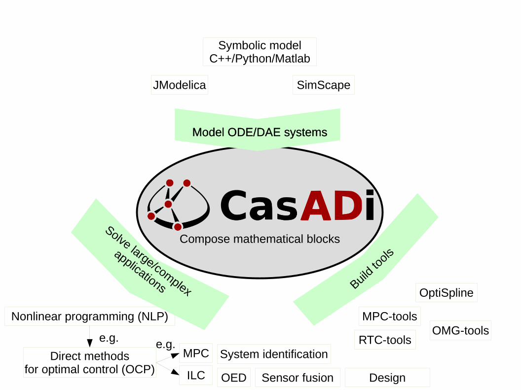
Compose mathematical blocks

JModelica SimScape

Symbolic modelC++/Python/Matlab

Nonlinear programming (NLP)

Direct methodsfor optimal control (OCP)

OptiSpline

MPC

ILC

Model ODE/DAE systemsModel ODE/DAE systems

Build

tools

Solve large/complex

applications

e.g. e.g.

MPC-tools

RTC-toolsSystem identification

OED

OMG-tools

Sensor fusion Design

Core

Core

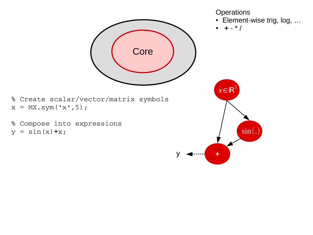
Operations● Element-wise trig, log, ...

% Create scalar/vector/matrix symbolsx = MX.sym('x',5);

% Compose into expressionsy = sin(x);

x∈ℝ5

sin (.)

. / .

y

Core

% Create scalar/vector/matrix symbolsx = MX.sym('x',5);

% Compose into expressionsy = sin(x)+x;

x∈ℝ5

sin ( .)

+

. / .y

Operations● Element-wise trig, log, …● + - * /

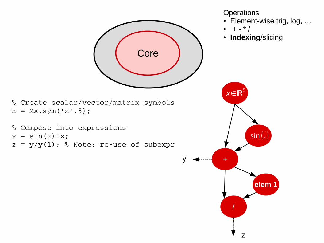
Core

% Create scalar/vector/matrix symbolsx = MX.sym('x',5);

% Compose into expressionsy = sin(x)+x;z = y/y(1); % Note: re­use of subexpr

x∈ℝ5

sin (.)

+

. / .

/

y

elem 1

z

Operations● Element-wise trig, log, …● + - * /● Indexing/slicing

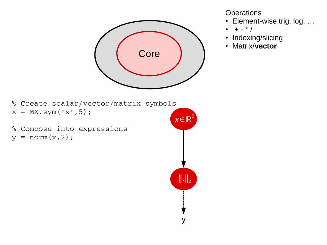
Core

% Create scalar/vector/matrix symbolsx = MX.sym('x',5);

% Compose into expressionsy = norm(x,2);

x∈ℝ5

‖.‖2

y

Operations● Element-wise trig, log, …● + - * /● Indexing/slicing● Matrix/vector

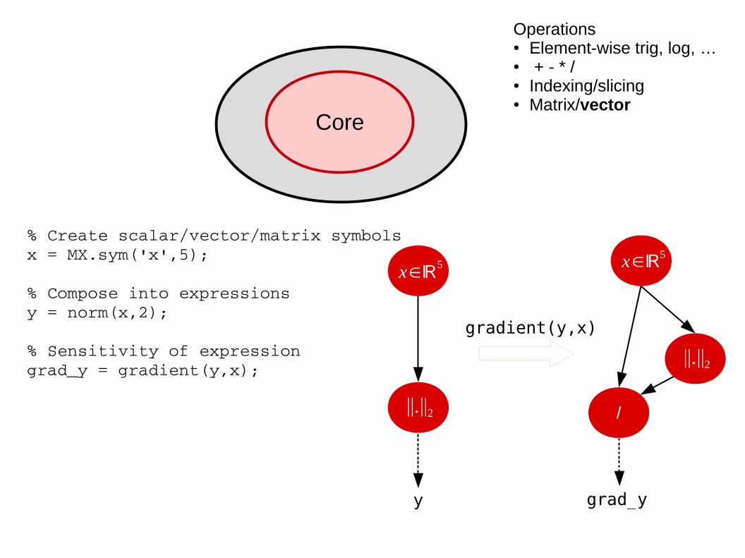
Core

% Create scalar/vector/matrix symbolsx = MX.sym('x',5);

% Compose into expressionsy = norm(x,2);

% Sensitivity of expressiongrad_y = gradient(y,x);

x∈ℝ5

‖.‖2

gradient(y,x)

x∈ℝ5

‖.‖2

/

. / .

y grad_y

Operations● Element-wise trig, log, …● + - * /● Indexing/slicing● Matrix/vector

grad_y = gradient(y,x);

CoreExpression graphs

Algorithmic differentiation

grad_y = gradient(y,x);

% Create a Function to evaluatef = Function('f',{x},{grad_y});f.generate('f.c');

CoreExpression graphs

Algorithmic differentiationC code-export (e.g. Matlab Mex/S-Function)

NLP

Conic

Integrator

Linea

r solve

Rootfinder

Interpolant

Custom

Expression graphs

Scalar Sparse matrix

Algorithmic differentiationC code-exportMulti-threadingMulti-processing

Lapack

Csparse

QPoases QRQP

HPMPC

Cplex

GurobiCLP

BlockSQP

SNOPT

IPOPT

SQP

Bonmin

Sundials Collocation Runge-Kutta

Newton

Kinsol

GPU mapreduce

Tensorflow

ADOLC

Linear

BSpline

WORHP

MA27

NLP ∂

Conic

Integrator ∂ ‡

Linea

r solve

∂ † ‡

Rootfinder ∂ ‡

Interpolant

∂ © † ‡

Custom

∂Expression graphs

Scalar Sparse matrix

∂ Algorithmic differentiation© C code-export† Multi-threading‡ Multi-processing

Lapack

Csparse ©

QPoases QRQP ©

HPMPC

Cplex

GurobiCLP

BlockSQP

SNOPT

IPOPT ‡

SQP ©

Bonmin

Sundials Collocation † Runge-Kutta †

Newton ©

Kinsol

GPU mapreduce

Tensorflow

ADOLC

Linear

BSpline

WORHP

MA27

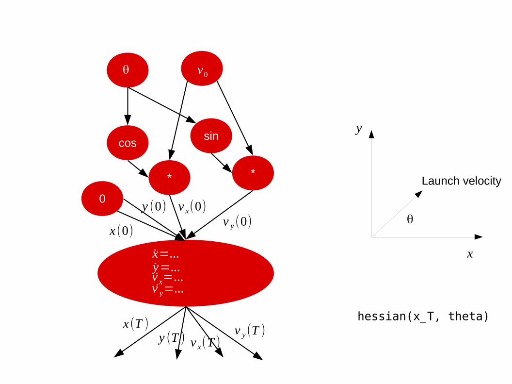
θ

x=...

hessian(x_T, theta)

v0

y=...v x=...v y=...

cossin

* *

0

x (0)

y (0) v x(0)v y (0)

x (T )y (T ) v x(T )

v y (T )

x

y

Launch velocity

θ

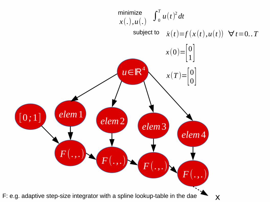
F: e.g. adaptive step-size integrator with a spline lookup-table in the dae

∫0

Tu(t )2 dtminimize

x(.) ,u(.)

subject to x(t )=f (x (t ) ,u(t )) ∀ t=0. .T

x(0)=[01]x(T )=[00]

u = opti.variable(N,1);

x = [0;1];for k=1:N  x = F(x,u(k));end

opti.minimize(u'*u);opti.subject_to(x==0);

opti.solver('ipopt');

sol = opti.solve();

sol.value(u)

Example: single-shooting

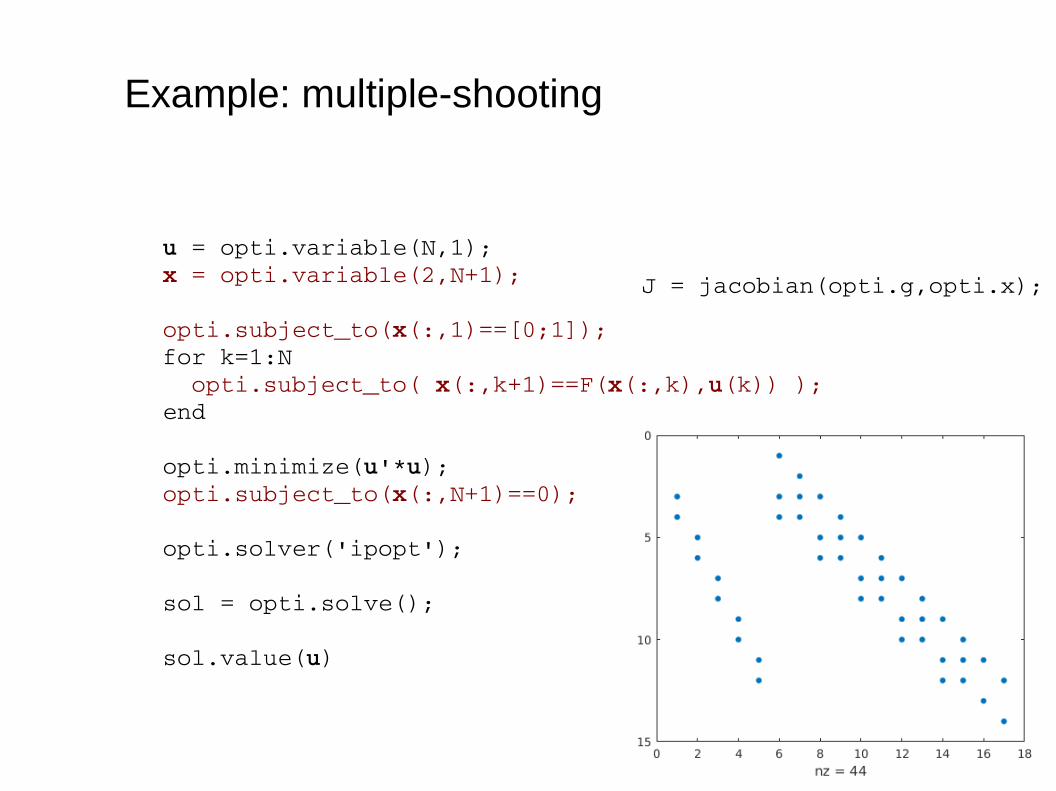
u = opti.variable(N,1);x = opti.variable(2,N+1);

opti.subject_to(x(:,1)==[0;1]);for k=1:N  opti.subject_to( x(:,k+1)==F(x(:,k),u(k)) );end

opti.minimize(u'*u);opti.subject_to(x(:,N+1)==0);

opti.solver('ipopt');

sol = opti.solve();

sol.value(u)

Example: multiple-shooting

J = jacobian(opti.g,opti.x);

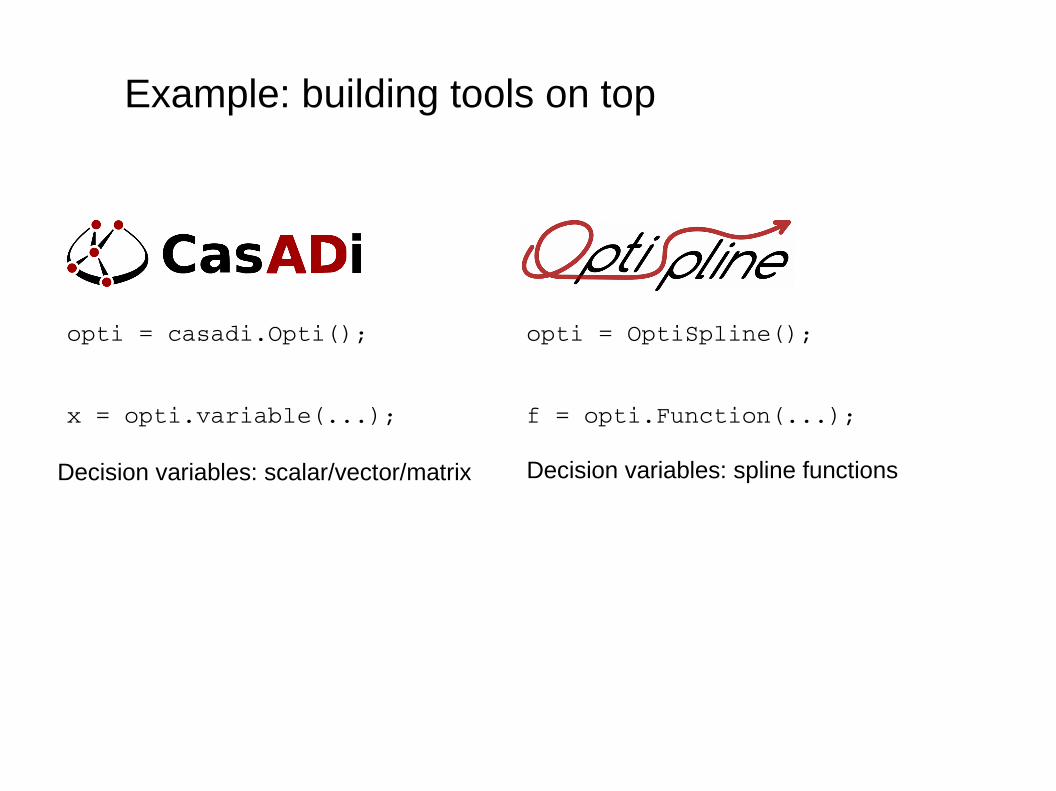
opti = casadi.Opti();

x = opti.variable(...);

Example: building tools on top

opti = OptiSpline();

f = opti.Function(...);

Decision variables: scalar/vector/matrix Decision variables: spline functions

● Open-souce LGPL● Multi-lingual: C++11/Matlab/Python● Build efficient optimal control solutions,

with minimal effort.Joel A. E. Andersson, Joris Gillis, Greg Horn, James B. Rawlings, Moritz Diehl,

“CasADi – A software framework for nonlinear optimization and optimal control,”

Mathematical Programming Computation, 2018.

http://casadi.org Workshop http://leuven2018.casadi.org