A theory for turbulent pipe and channel flows
31
J. Fluid Mech. (2000), vol. 421, pp. 115–145. Printed in the United Kingdom c 2000 Cambridge University Press 115 A theory for turbulent pipe and channel flows By MARTIN WOSNIK 1 , LUCIANO CASTILLO 2 AND WILLIAM K. GEORGE 3 1 State University of New York at Buffalo, Buffalo, NY 14260, USA 2 Rensselaer Polytechnic Institute, Troy, NY 12180, USA 3 Department of Thermo and Fluid Dynamics, Chalmers University of Technology, 412 96 G¨ oteborg, Sweden (Received 28 January 1998 and in revised form 14 February 2000) A theory for fully developed turbulent pipe and channel flows is proposed which extends the classical analysis to include the effects of finite Reynolds number. The proper scaling for these flows at finite Reynolds number is developed from dimensional and physical considerations using the Reynolds-averaged Navier–Stokes equations. In the limit of infinite Reynolds number, these reduce to the familiar law of the wall and velocity deficit law respectively. The fact that both scaled profiles describe the entire flow for finite values of Reynolds number but reduce to inner and outer profiles is used to determine their functional forms in the ‘overlap’ region which both retain in the limit. This overlap region corresponds to the constant, Reynolds shear stress region (30 <y + < 0.1R + approximately, where R + = u * R/ν ). The profiles in this overlap region are logarithmic, but in the variable y + a where a is an offset. Unlike the classical theory, the additive parameters, B i , B o , and log coefficient, 1/κ, depend on R + . They are asymptotically constant, however, and are linked by a constraint equation. The corresponding friction law is also logarithmic and entirely determined by the velocity profile parameters, or vice versa. It is also argued that there exists a mesolayer near the bottom of the overlap region approximately bounded by 30 <y + < 300 where there is not the necessary scale separation between the energy and dissipation ranges for inertially dominated turbulence. As a consequence, the Reynolds stress and mean flow retain a Reynolds number dependence, even though the terms explicitly containing the viscosity are negligible in the single-point Reynolds-averaged equations. A simple turbulence model shows that the offset parameter a accounts for the mesolayer, and because of it a logarithmic behaviour in y applies only beyond y + > 300, well outside where it has commonly been sought. The experimental data from the superpipe experiment and DNS of channel flow are carefully examined and shown to be in excellent agreement with the new theory over the entire range 1.8 × 10 2 <R + < 5.3 × 10 5 . The Reynolds number dependence of all the parameters and the friction law can be determined from the single empirical function, H = A/(ln R + ) α for α> 0, just as for boundary layers. The Reynolds num- ber dependence of the parameters diminishes very slowly with increasing Reynolds number, and the asymptotic behaviour is reached only when R + 10 5 .
Transcript of A theory for turbulent pipe and channel flows

J. Fluid Mech. (2000), vol. 421, pp. 115–145. Printed in the United Kingdom
c© 2000 Cambridge University Press
115
A theory for turbulent pipe and channel flows
By M A R T I N W O S N I K1, L U C I A N O C A S T I L L O2
AND W I L L I A M K. G E O R G E3
1State University of New York at Buffalo, Buffalo, NY 14260, USA2Rensselaer Polytechnic Institute, Troy, NY 12180, USA
3Department of Thermo and Fluid Dynamics, Chalmers University of Technology,412 96 Goteborg, Sweden
(Received 28 January 1998 and in revised form 14 February 2000)
A theory for fully developed turbulent pipe and channel flows is proposed whichextends the classical analysis to include the effects of finite Reynolds number. Theproper scaling for these flows at finite Reynolds number is developed from dimensionaland physical considerations using the Reynolds-averaged Navier–Stokes equations.In the limit of infinite Reynolds number, these reduce to the familiar law of the walland velocity deficit law respectively.
The fact that both scaled profiles describe the entire flow for finite values ofReynolds number but reduce to inner and outer profiles is used to determine theirfunctional forms in the ‘overlap’ region which both retain in the limit. This overlapregion corresponds to the constant, Reynolds shear stress region (30 < y+ < 0.1R+
approximately, where R+ = u∗R/ν). The profiles in this overlap region are logarithmic,but in the variable y+ a where a is an offset. Unlike the classical theory, the additiveparameters, Bi, Bo, and log coefficient, 1/κ, depend on R+. They are asymptoticallyconstant, however, and are linked by a constraint equation. The corresponding frictionlaw is also logarithmic and entirely determined by the velocity profile parameters, orvice versa.
It is also argued that there exists a mesolayer near the bottom of the overlapregion approximately bounded by 30 < y+ < 300 where there is not the necessaryscale separation between the energy and dissipation ranges for inertially dominatedturbulence. As a consequence, the Reynolds stress and mean flow retain a Reynoldsnumber dependence, even though the terms explicitly containing the viscosity arenegligible in the single-point Reynolds-averaged equations. A simple turbulence modelshows that the offset parameter a accounts for the mesolayer, and because of it alogarithmic behaviour in y applies only beyond y+ > 300, well outside where it hascommonly been sought.
The experimental data from the superpipe experiment and DNS of channel floware carefully examined and shown to be in excellent agreement with the new theoryover the entire range 1.8× 10² < R+ < 5.3× 10⁵. The Reynolds number dependenceof all the parameters and the friction law can be determined from the single empiricalfunction, H = A/(lnR+)α for α > 0, just as for boundary layers. The Reynolds num-ber dependence of the parameters diminishes very slowly with increasing Reynoldsnumber, and the asymptotic behaviour is reached only when R+ � 105.

116 M. Wosnik, L. Castillo and W. K. George
1. IntroductionPipe and channel flows have recently become the subject of intense scrutiny, thanks
in part to new experimental data which has become available from the superpipeexperiment at Princeton (Zagarola 1996; Zagarola & Smits 1998a). In spite of thefacts that the scaling laws for pipe and channel flows were established more than 80years ago (Stanton & Pannell 1914; Prandtl 1932) and that the now classical theory ofMillikan was offered in 1938 for the friction law and velocity profiles, the subject hasremained of considerable interest. Examples from the last 30 years alone include theanalyses of Tennekes (1968), Bush & Fendell (1974), Long & Chen (1981), and Panton(1990). All of these were essentially refinements of the original Millikan theory inwhich the essential functional form of the friction and velocity laws was logarithmic,and only the infinite Reynolds number state was considered. The difficulties presentedby the experimental data have recently been extensively reviewed by Gad-el-Hak &Bandyopadhyay (1994).
Barenblatt and coworkers (Barenblatt 1993, 1996; Barenblatt & Prostokishin 1993;Barenblatt, Chorin & Prostokishin 1997) have suggested that the velocity profiles ofpipe, channel and boundary layer flows are power laws. By contrast, George andcoworkers (George 1988, 1990, 1995; George & Castillo 1993, 1997; George, Knecht& Castillo 1992; George, Castillo & Knecht 1996; George, Castillo & Wosnik 1997)have argued that the overlap velocity profiles and friction law for boundary layersare power laws, but that the corresponding relations for pipes and channels arelogarithmic.
Specifically, for boundary layers George & Castillo (1997 hereafter referred toas GC), used the Reynolds-averaged Navier–Stokes equations and an asymptoticinvariance principle (AIP) to deduce that the proper velocity scale for the outer partwas U∞, the free-stream velocity. In the inner region, however, the proper velocityscale was u∗, the friction velocity, just as in the classical law of the wall. Since theratio u∗/U∞ varied with Reynolds number, so did the velocity profiles in the Reynoldsnumber dependent overlap region. These were derived using near asymptotics as
U
u∗= Ci(y
+ + a+)γ (1.1)
andU
U∞= Co(y + a)γ, (1.2)
where y+ = y/η, η = ν/u∗, y = y/δ where δ is the boundary layer thickness (chosen asδ0.99 for convenience). This overlap region was shown to correspond to the region ofconstant Reynolds stress of the flow, approximately 30 < y+ < 0.1δ+. The parameter arepresents an origin shift, and was shown to be related to the existence of a mesolayerin the region approximately given by 30 < y+ < 300 in which the dissipative scalesare not fully separated from the energy and Reynolds stress producing ones.
The parameters Ci, Co, and γ were functions of δ+, were asymptotically constant,and satisfied the constraint equation,
ln δ+ dγ
d ln δ+=
d lnCo/Cid ln δ+
(1.3)
where δ+ = u∗δ/ν. The friction law was given by
u∗U∞
=Co
Ci(δ+)−γ. (1.4)

A theory for turbulent pipe and channel flows 117
The constraint equation was transformed by defining a single new functionh = h(ln δ+)
lnCo/Ci = (γ − γ∞) ln δ+ + h (1.5)
and
γ − γ∞ = − dh
d ln δ+. (1.6)
The function h− h∞ was determined empirically to be given by
h(δ+)− h∞ =A
(ln δ+)α, (1.7)
where h∞ = ln(Co∞/Ci∞) and α > 1 is a necessary condition. (Note that this can beshown to be the leading term in an expansion of the exact solution.)
It followed immediately that
γ − γ∞ =αA
(ln δ+)1+α, (1.8)
Co
Ci=Co∞Ci∞
exp[(1 + α)A/(ln δ+)α] (1.9)
andu∗U∞
=Co∞Ci∞
(δ+)−γ∞ exp[A/(ln δ+)α]. (1.10)
The values for the constants were determined from the data to be γ∞ = 0.0362,Co∞/Ci∞ = exp(h∞) = 0.0163, Co ≈ Co∞ = 0.897 (so Ci∞ = 55), A = 2.9, and α = 0.46.Also it was established from the available data that a+ was nearly constant andapproximately equal to −16.
The purpose of this paper is to apply the same methodology to pipe and channelflows, and to compare the resulting theory with the new experimental data. Theimportant difference from previous efforts mentioned above will be seen to be thatthe effects of finite Reynolds number are explicitly included and the mesolayer isaccounted for.
2. Scaling laws for turbulent pipe and channel flowThe streamwise momentum equation for a fully developed two-dimensional channel
flow at high Reynolds number reduces to
0 = −1
ρ
dP
dx+
∂
∂y
[〈−uv〉+ ν
∂U
∂y
]. (2.1)
Like the boundary layer, the viscous term is negligible everywhere except very nearthe wall, so that the core (or outer) flow in the limit of infinite Reynolds number isexactly governed by
0 = −1
ρ
dP
dx+
∂
∂y〈−uv〉. (2.2)
In the limit of infinite Reynolds number, the inner layer is exactly governed by
0 =∂
∂y
[〈−uv〉+ ν
∂U
∂y
]. (2.3)
118 M. Wosnik, L. Castillo and W. K. George
This can be integrated from the wall to obtain the total stress
u2∗ = 〈−uv〉+ ν
∂U
∂y, (2.4)
where u∗ is the friction velocity defined as u2∗ ≡ τw/ρ. As the distance from the wallis increased, the viscous stress vanishes and 〈−uv〉 → u2∗, but only in the infiniteReynolds number limit. At finite Reynolds numbers the pressure gradient causes thetotal stress to drop linearly until it reaches zero at the centre of the channel (or pipe).Hence the Reynolds stress never really reaches the value of u2∗, but instead reaches amaximum value away from the wall before dropping slowly as distance from the wallis increased.
It is obvious that the inner profiles must scale with u∗ and ν since these are theonly parameters in the inner equations and boundary conditions. Hence, there mustbe a law of the wall (at least for a limited region very close to the wall). This shouldnot be taken to imply, however, that u2∗ is an independent parameter; it is not. It isuniquely determined by the pressure drop imposed on the pipe, the pipe diameterand the kinematic viscosity.
Because there is no imposed condition on the velocity, except for the no-slipcondition at the wall, an outer scaling velocity must be sought from the parametersin the outer equation itself. Since there are only two, −(1/ρ)dP/dx, the externallyimposed pressure gradient, and R, the channel half-width, only a single velocity canbe formed, namely
Uo =
(−Rρ
dP
dx
)1/2
. (2.5)
Unlike the developing boundary layer, the fully developed pipe or channel flow ishomogeneous in the streamwise direction, so the straightforward similarity analysisof GC using the x-dependence to establish the scaling parameters is not possible.However, because of this streamwise homogeneity, there is an exact balance betweenthe wall shear stress acting on the walls, and the net pressure force acting across theflow. For fully developed channel flow, this equilibrium requires that
u2∗ = −R
ρ
dP
dx. (2.6)
which is just the square of equation (2.5) above; thus, Uo = u∗. Therefore, the outerscale velocity is also u∗, and the outer and inner velocity scales are the same. Thefactor of 2 which appears in the corresponding pipe flow force balance can be ignoredin choosing the scale velocity, so the same argument and result apply to it as well.
Thus channel and pipe flows differ from boundary layer flows where asymptoticReynolds number independence and streamwise inhomogeneity demand that the innerand outer scales for the mean velocity be different (GC). This consequence of thestreamwise homogeneity for the governing equations themselves is fundamental tounderstanding the unique nature of pipe and channel flows. Homogeneity causes theinner and outer velocity scale to be the same, and this in turn is the reason why theseflows show a logarithmic dependence for the velocity in the overlap region and forthe friction law. This can be contrasted with boundary layers, where the inner andouter velocity scales are different because of their inhomogeneity in x, and hence arecharacterized by power laws.
The analysis presented below will be based on using u∗ as the outer velocity scale;however, it should be noted before leaving this section that there are at least two

A theory for turbulent pipe and channel flows 119
other possibilities which might be considered for an outer velocity scale. Both areformed from the mass-averaged velocity defined for the pipe by
Um ≡ 1
πR2
∫ R
0
Urdr. (2.7)
The first possibility is to use Um directly, the second is to use its difference fromthe centreline velocity, Uc − Um. The former has an advantage in that it is ofteneasier to specify the mass flow in experiments and simulations than the pressure drop(or shear stress), but it has the disadvantage that it does not lend itself easily tothe overlap analysis described below. The latter has been utilized with great successby Zagarola & Smits (1998b) in removing the Reynolds number dependence of thevelocity profiles in both boundary layers and pipe flows. For the purpose of this paperit is sufficient to note that in the limit as R+ = u∗R/ν → ∞, Uc − Um → const × u∗.Hence the fundamental limiting and overlap arguments of the succeeding sectionswill be the same for both u∗ and Uc −Um; only the Reynolds number dependence ofthe coefficients will differ.
3. Finite versus infinite Reynolds numberFrom the dimensional/physical analysis above, it follows that appropriate inner-
and outer-scaled versions of the velocity profile can be defined as two families ofcurves with parameter R+, i.e.
U
u∗= fi(y
+, R+) (3.1)
andU −Uc
u∗= fo(y, R
+), (3.2)
where the outer velocity has been referenced to the velocity at the centreline, Uc, toavoid the necessity of accounting for viscous effects over the inner layer when thelimits are taken later. The outer length scale is some measure of the diameter of thepipe (say the pipe radius) or the width of the channel (say half-width). Both of thesewill be denoted as R in the remainder of the paper.
Since the length scales for inner and outer profiles are different, no single scalinglaw should be able to collapse data for the entire flow. The ratio of length scalesis a Reynolds number, R+ = Ru∗/ν, therefore the region between the two similarityregimes cannot be Reynolds number independent, except possibly in the limit ofinfinite Reynolds number. Moreover, since the neglected terms in both inner andouter equations depend on the ratio of length scales (see Tennekes & Lumley 1972),then neither set of scaling parameters will be able to perfectly collapse the data ineither region at finite values of R+.
The actual mean velocity profile at finite Reynolds number is the average of theinstantaneous solutions to the Navier–Stokes equations and boundary conditions.This profile, whether determined from a real flow by measurement, a direct numericalsimulation, or not at all, exists, at least in principle, and is valid everywhere regardlessof how it is scaled. Therefore it is important to note that both families of curvesdescribed by equations (3.1) and (3.2), fi(y
+, R+) and fo(y, R+), represent the entire
velocity profile, at least as long as the dependence on R+ is retained (as long as R+
is finite). In other words, they represent the same solutions, and have simply beenscaled differently.

120 M. Wosnik, L. Castillo and W. K. George
40
30
20
10
0100 102 104 106
y+
Superpipe data, 8.5 ×10² <R+ <5.3 ×10⁵
u+ = y+
U/u
*
Figure 1. Velocity profiles in inner variables.
10–2
Superpipe data, 8.5 ×10² <R+ <5.3 ×10⁵
20
15
10
5
0
–510–1 100
y/R
(Uc–U
)/u *
Figure 2. Velocity profiles in outer variables.
Properly scaled profiles must, by the asymptotic invariance principle (AIP, George1995), become asymptotically independent of R+ in the limit of infinite Reynoldsnumber, i.e.
lim fi(y+, R+)→ fi∞(y+),
lim fo(y, R+)→ fo∞(y)
as R+ → ∞. Otherwise an inner and outer scaling makes no sense. In fact, theselimiting profiles should be solutions to the inner and outer equations respectively (i.e.equations (2.3) and (2.2)), which are themselves valid only in the infinite Reynoldsnumber limit.
Figures 1 and 2 show the mean velocity profile data from the Princeton super-pipe experiment (Zagarola 1996; Zagarola & Smits 1998a) in both inner and outervariables. Note the excellent collapse very close to the wall for y+ < 100 in inner vari-ables, and over the core region for y > 0.3. Note also that the region of approximatecollapse in inner variables (figure 1) increases from the wall with increasing Reynoldsnumber, as does the inward extent of the outer variable collapse (figure 2). In fact,the parameter R+ uniquely labels the fanning out of the inner-scaled profiles in theouter region and the outer-scaled profiles near the wall in figures 1 and 2.
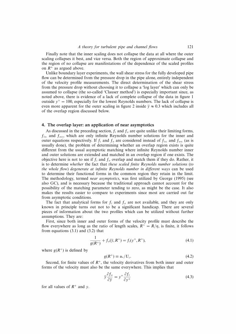
A theory for turbulent pipe and channel flows 121
Finally note that the inner scaling does not collapse the data at all where the outerscaling collapses it best, and vice versa. Both the region of approximate collapse andthe region of no collapse are manifestations of the dependence of the scaled profileson R+ as argued above.
Unlike boundary layer experiments, the wall shear stress for the fully developed pipeflow can be determined from the pressure drop in the pipe alone, entirely independentof the velocity profile measurements. The direct determination of the shear stressfrom the pressure drop without choosing it to collapse a ‘log layer’ which can only beassumed to collapse (the so-called ‘Clauser method’) is especially important since, asnoted above, there is evidence of a lack of complete collapse of the data in figure 1outside y+ = 100, especially for the lowest Reynolds numbers. The lack of collapse iseven more apparent for the outer scaling in figure 2 inside y ≈ 0.3 which includes allof the overlap region discussed below.
4. The overlap layer: an application of near asymptoticsAs discussed in the preceding section, fi and fo are quite unlike their limiting forms,
fi∞ and fo∞, which are only infinite Reynolds number solutions for the inner andouter equations respectively. If fi and fo are considered instead of fi∞ and fo∞ (as isusually done), the problem of determining whether an overlap region exists is quitedifferent from the usual asymptotic matching where infinite Reynolds number innerand outer solutions are extended and matched in an overlap region if one exists. Theobjective here is not to see if fi and fo overlap and match them if they do. Rather, itis to determine whether the fact that these scaled finite Reynolds number solutions (tothe whole flow) degenerate at infinite Reynolds number in different ways can be usedto determine their functional forms in the common region they retain in the limit.The methodology, termed near asymptotics, was first utilized by George (1995) (seealso GC), and is necessary because the traditional approach cannot account for thepossibility of the matching parameter tending to zero, as might be the case. It alsomakes the results easier to compare to experiments since most are carried out farfrom asymptotic conditions.
The fact that analytical forms for fi and fo are not available, and they are onlyknown in principle turns out not to be a significant handicap. There are severalpieces of information about the two profiles which can be utilized without furtherassumptions. They are:
First, since both inner and outer forms of the velocity profile must describe theflow everywhere as long as the ratio of length scales, R+ = R/η, is finite, it followsfrom equations (3.1) and (3.2) that
1
g(R+)+ fo(y, R
+) = fi(y+, R+), (4.1)
where g(R+) is defined by
g(R+) ≡ u∗/Uc. (4.2)
Second, for finite values of R+, the velocity derivatives from both inner and outerforms of the velocity must also be the same everywhere. This implies that
y∂fo
∂y= y+ ∂fi
∂y+(4.3)
for all values of R+ and y.

122 M. Wosnik, L. Castillo and W. K. George
Third, as noted above, in the limit both fo and fi must become asymptoticallyindependent of R+, i.e. fo(y, R
+)→ fo∞(y) and fi(y+, R+)→ fi∞(y+) as R+ →∞.
Now the problem is that in the limit as R+ →∞, the outer form fails to account forthe behaviour close to the wall while the inner form fails to describe the behaviouraway from it. The question is: In this limit (as well as for all finite values approachingit) does there exist an ‘overlap’ region where equation (4.1) is still valid? (Note thatboundary layer flows are quite different from pipe and channel flows since the overlaplayer in the latter remains at fixed distance from the wall for all x because of thestreamwise homogeneity, as long as the external parameters – like geometry andReynolds number – are fixed, while in the former it moves away from the wall withincreasing x.)
The question of whether there is a common region of validity can be investigatedby examining how rapidly fo and fi are changing with R+, or more conveniently withlnR+. The relative variation of fi and fo with Reynolds number can be related totheir Taylor series expansion about a fixed value of R+, i.e.
fi(y+;R+ + ∆R+)− fi(y+;R+)
∆ lnR+fi(y+, R+)≈ 1
fi(y+, R+)
∂fi(y+;R+)
∂ lnR+
∣∣∣∣y+
≡ Si(R+, y+) (4.4)
andfo(y;R+ + ∆R+)− fo(y;R+)
∆ lnR+fo(y, R+)≈ 1
fo(y, R+)
∂fo(y;R+)
∂ lnR+
∣∣∣∣y
≡ So(R+, y). (4.5)
Thus Si and So are measures of the Reynolds number dependence of fi and fo,respectively. Both vanish identically in the limit as lnR+ → ∞. If y+
max denotes alocation where outer flow effects begin to be strongly felt on the inner-scaled profile,then for y+ < y+
max, Si should be much less than unity (or else the inner scaling is notvery useful). Similarly, if ymin measures the location where viscous effects begin to bestrongly felt (e.g. as the linear velocity region near the wall is approached), then Soshould be small for y > ymin. Obviously either Si or So should increase as these limitsare approached. Outside these limits, one or the other should increase dramatically.
The quantities Si and So can, in fact, be used to provide a formal definition of an‘overlap’ region where both scaling laws are valid. Since Si will increase drasticallyfor large values of y for given lnR+, and So will increase for small values of y, an‘overlap’ region exists only if there is a region for which both Si and So remain smallsimultaneously. In the following paragraphs, this condition will be used in conjunctionwith equation (4.1) to derive the functional form of the velocity in the overlap regionat finite Reynolds number, hence the term ‘near asymptotics’.
Because the overlap region moves toward the wall with increasing R+, it isconvenient and necessary to introduce an intermediate variable y which can befixed in the overlap region all the way to the limit, regardless of what is happeningin physical space (see Cole & Kevorkian 1981). A definition of y which accomplishesthis is given by
y = y+R+−n (4.6)
or
y+ = yR+n. (4.7)
Since R+ = y+/y, it follows that
y = yR+n−1. (4.8)
For all values of n satisfying 0 < n < 1, y can remain fixed in the limit as R+ → ∞

A theory for turbulent pipe and channel flows 123
while y → 0 and y+ → ∞. Substituting these into equation (4.1) yields the matchingcondition on the velocity in terms of the intermediate variable:
1
g(R+)+ fo(R
+n−1y, R+) = fi(R
+ny, R+). (4.9)
Now equation (4.9) can be differentiated with respect to R+ for fixed y to yieldequations which explicitly include Si and So. The result after some manipulation is
y∂fo
∂y
∣∣∣∣R+
=1
κ− [Si(y+, R+)fi(y
+, R+)− So(y, R+)fo(y, R+)], (4.10)
where1
κ(R+)≡ −R
+
g2
dg
dR+=
d(1/g)
d lnR+. (4.11)
The first term on the right-hand side of equation (4.10) is at most a function of R+
alone, while the second term contains all of the residual y-dependence.Now it is clear that if both
|So| fo � 1/κ (4.12)
and|Si| fi � 1/κ (4.13)
then the first term on the right-hand side of equation (4.10) dominates. If 1/κ → 0,the inequalities are still satisfied as long as the left-hand side of equations (4.12)and (4.13) does so more rapidly than 1/κ. Note that a much weaker condition can beapplied which yields the same result, namely that both inner and outer scaled profileshave the same dependence on R+, i.e. Sifi = Sofo in the overlap range so only 1/κremains. If these inequalities are satisfied over some range in y, then to leading order,equation (4.10) can be written as
y∂fo
∂y
∣∣∣∣R+
=1
κ. (4.14)
The solution to equation (4.14) could be denoted as f(1)o since it represents a first-
order approximation to fo. Because 1/κ depends on R+ it is not simply the sameas fo∞, but reduces to it in the limit. Thus, by regrouping all of the y-independentcontributions into the leading term, the method applied here has yielded a moregeneral result than the customary expansion about infinite Reynolds number. (It isalso easy to see why the usual matching of infinite Reynolds number inner and outersolutions will not work if the limiting value of 1/κ is zero, which cannot yet be ruledout.)
From equations (4.3) and (4.14), it follows that
y+ ∂fi
∂y+
∣∣∣∣R+
=1
κ. (4.15)
Equations (4.14) and (4.15) must be independent of the origin for y; hence theymust be invariant to transformations of the forms y → y + a and y+ → y+ + a+,respectively, where a is at most a function of the Reynolds number. Therefore themost general forms of equations (4.14) and (4.17) are
(y + a)∂fo
∂(y + a)
∣∣∣∣R+
=1
κ(4.16)

124 M. Wosnik, L. Castillo and W. K. George
and
(y+ + a+)∂fi
∂(y+ + a+)
∣∣∣∣R+
=1
κ. (4.17)
The solutions to these overlap equations are given by
U −Uc
u∗= fo(y, R
+) =1
κ(R+)ln [y + a(R+)] + Bo(R
+) (4.18)
andU
u∗= fi(y
+, R+) =1
κ(R+)ln [y+ + a+(R+)] + Bi(R
+). (4.19)
The superscript (1) has been dropped; however it is these first-order solutions thatare being referred to unless otherwise stated. Thus the velocity profiles in the overlapregion are logarithmic, but with parameters which are in general Reynolds numberdependent.
Note that the particular form of the solution ln(y + a) has also been identified byOberlack (1997) from a Lie group analysis of the equations governing homogeneousshear flows. It will be argued in § 8 that a+ is closely related to the mesolayer, justas it is for the boundary layer (GC). The data will be found to be consistent witha+ ≈ −8. Interestingly, the need for the offset parameter a appears to have first beennoticed by Squire (1948) (see also Duncan, Thom & Young 1970) using a simpleeddy viscosity model. (Even his value of a+ = 5.9 does not differ much from the oneused here.) George et al. (1996) arrived at a similar form from a simple one-equationturbulence model for the mesolayer, as discussed in § 8 below.
A particularly interesting feature of these first-order solutions is that the inequal-ities given by equations (4.12) and (4.13) determine the limits of validity of bothequations (4.16) and (4.17) since either So or Si will be large outside the overlapregion. Clearly, the extent of this region will increase as the Reynolds number (orR+) increases.
The parameters 1/κ, Bi and Bo must be asymptotically constant since they occurin solutions to equations which are themselves Reynolds number independent in thelimit (AIP). Moreover, the limiting values, κ∞, Bi∞, and Bo∞ cannot all be zero, orelse the solutions themselves are trivial. In the limit of infinite Reynolds number theenergy balance in the overlap region reduces to production equals dissipation, i.e.ε+ = P+. In § 8 this will be shown to imply that
ε+ → du+
dy+=
1
κ(y+ + a+). (4.20)
Since the local energy dissipation rate must be finite and non-zero (Frisch 1995),it follows that 1/κ∞ must be finite and non-zero. It will be shown below thatthese conditions severely restrict the possible Reynolds number dependences for theparameters κ, Bi and Bo. (Note that the same physical constraint on the boundarylayer results requires the power exponent, γ, to be asymptotically finite and non-zero.)
The relation between u∗ and Uc follows immediately from equation (4.1), i.e.
Uc
u∗=
1
g(R+)=
1
κ(R+)lnR+ + [Bi(R
+)− Bo(R+)]. (4.21)
Thus the friction law is entirely determined by the velocity parameters forthe overlap region. However, equation (4.11) must also be satisfied. Substituting

A theory for turbulent pipe and channel flows 125
equation (4.21) into equation (4.11) implies that κ, Bi, and Bo are constrained by
lnR+ d(1/κ)
d lnR+= −d(Bi − Bo)
d lnR+. (4.22)
This is exactly the criterion for the neglected terms in equation (4.10) to vanishidentically (i.e. Sifi−Sofo ≡ 0). Therefore the solution represented by equations (4.18)to (4.22) is, indeed, the first-order solution for the velocity profile in the overlap layerat finite, but large, Reynolds number. Clearly when y+ is too big or y is too small fora given value of R+, the inequalities of equations (4.12) and (4.13) cannot be satisfied.Since all the derivatives with respect to R+ must vanish as R+ → ∞ (AIP), the outerrange of the inner overlap solution is unbounded in the limit, while the inner rangeof the outer one is bounded only by y = −a.
Equation (4.22) is invariant to transformations of the form R+ → DsR+ where Ds
is a scale factor which ensures that the functional dependence is independent of theparticular choice of the outer length scale (e.g. diameter versus radius). Thus the ve-locity profile in the overlap layer is logarithmic, but with parameters which depend onthe Reynolds number, DsR
+. The functions κ(DsR+), Bi(DsR
+) and Bo(DsR+) must be
determined either empirically or from a closure model for the turbulence. Regardlessof how they are determined, the results must be consistent with equation (4.22).
5. A solution for the Reynolds number dependenceFrom equation (4.22) it is clear that if either Bi − Bo or 1/κ are given, then the
other is determined (to within an additive constant). Since there is only one unknownfunction, it is convenient to transform equation (4.22) using the function
H(DsR+) ≡
(1
κ− 1
κ∞
)lnDsR
+ + (Bi − Bo), (5.1)
where H = H(DsR+) remains to be determined. If H(DsR
+) satisfies
1
κ− 1
κ∞=
dH
d lnDsR+(5.2)
then equation (4.22) is satisfied. It follows immediately that
1
g=Uc
u∗=
1
κ∞lnDsR
+ +H(DsR+). (5.3)
Thus the Reynolds number dependence of the single function H(DsR+) determines
that of κ, Bi − Bo and g.The conditions that both Bi∞ and Bo∞ be finite and non-zero require that:
eitherBi, Bo and κ remain constant always;
or(i) 1/κ→ 1/κ∞ faster than 1/ lnDsR
+ → 0, and(ii) H(DsR
+)→ H∞ = constant.Obviously from equation (5.1),
H∞ = Bi∞ − Bo∞. (5.4)
It is also clear from the constraint equation that the natural variable is lnDsR+.
Since this blows up in the limit as R+ →∞, H can at most depend on inverse powers

126 M. Wosnik, L. Castillo and W. K. George
of lnDsR+. Thus the expansion of H for large values of lnDsR
+ must be of the form
H(DsR+)−H∞ =
A
[lnDsR+]α
[1 +
A1
lnDsR++
A2
(lnDsR+)2+ · · ·
]. (5.5)
Note that conditions (i) and (ii) above imply that α > 0. Although only the leadingterm will be found to be necessary to describe the data, the rest will be carried indeveloping the theoretical relations below.
Substituting equation (5.5) in equation (5.3) yields
Uc
u∗=
1
κ∞lnDsR
+ +[Bi∞−Bo∞]+A
[lnDsR+]α
[1 +
A1
lnDsR++
A2
(lnDsR+)2+ · · ·
]. (5.6)
As R+ →∞ this reduces to the classical solution of Millikan (1938). This is reassuringsince Millikan’s analysis is an infinite Reynolds number analysis of inner and outerprofiles scaled in the same way. (Note that this was not true for the boundarylayer: the Clauser/Millikan analysis assumed the same scaling laws applied as for thechannel/pipe. George & Castillo argued from the Reynolds-averaged equations thatthey had to be different, hence the different conclusions.)
The Reynolds number variation of 1/κ and Bi − Bo can be obtained immediatelyfrom equations (5.1), (5.2) and (5.5) as
1
κ− 1
κ∞= − αA
(lnDsR+)1+α
[1 +
(1 + α
α
)A1
lnDsR++
(2 + α
α
)A2
(lnDsR+)2+ · · ·
](5.7)
and
(Bi − Bo)− (Bi∞ − Bo∞)
=(1 + α)A
(lnDsR+)α
[1 +
(2 + α
1 + α
)A1
lnDsR++
(3 + α
1 + α
)A2
(lnDsR+)2+ · · ·
]. (5.8)
Figure 3 shows the friction data of the superpipe experiment of Zagarola & Smits(1998a). As the investigators themselves have pointed out, careful scrutiny revealsthat the data do not fall on a straight line on a semi-log plot, so a simple logarithmicfriction law with constant coefficients does not describe all the data to within theaccuracy of the data itself. In particular, a log which attempts to fit all of the datadips away from it in the middle range. On the other hand, a log law which fits thehigh Reynolds number range does not fit the low, or vice versa. Figure 3 shows twocurves: the first represents a regression fit of equation (5.6) with only the leading term(i.e. A1 = A2 = 0), while the second shows only the asymptotic log form of equation(5.6). The former provides an excellent fit to the data for all Reynolds numbersand asymptotes exactly to the latter, but only at much higher Reynolds numbers.The differences, although slight, are very important since they entirely determine (orreflect) the Reynolds number dependence of the parameters 1/κ, Bi and Bo. Thelast of these will be seen later to be especially sensitive to this dependence. Clearlythe simplest of the proposed forms of H captures the residual Reynolds numberdependence, while simply using constant coefficients does not.
The values obtained for the asymptotic friction law parameters using optimizationtechniques are κ∞ = 0.447, Bi∞ − Bo∞ = 8.45, while those describing the Reynoldsnumber dependence are A = −0.668 and α = 0.441. The higher-order terms inequation (5.5) were ignored, and will be throughout the remainder of this paper. Thesame optimization techniques showed no advantage in using values of the parameterDs different from unity, hence Ds = 1 to within experimental error. Note that the

A theory for turbulent pipe and channel flows 127
Superpipe dataTheory, eqn (5.6)Uc/u*= (1/κinf) In (R+)+ Hinf
40
3535
30
25
20103 104 105 106
R+
40
35
30
25
20
Superpipe dataTheory, eqn (5.6)Uc/u*= (1/κinf) In (R+)+ Hinf
0 1 2 3 4 6
Uc /u*
Uc /u*
R+
Figure 3. Variation of Uc/u∗ with R+ = Ru∗/ν.
values of Bi∞ and Bo∞ cannot be determined individually from the friction data,only their difference. Nominal values for κ and Bi − Bo are approximately 0.445 and8.20 respectively, the former varying by less than 0.5% and the latter by only 1%over the entire range of the data. These values differ only slightly from the valuesdetermined by Zagarola (1996) (0.44 and 7.8, respectively) and Zagarola & Smits(1998a) (0.436 and 7.66, respectively) using the velocity profiles alone and assumingthat the asymptotic state had been reached. In fact it will be shown later from thevelocity profiles that Bi is independent of Reynolds number and approximately equalto 6.5. Thus only Bo significantly changes with Reynolds number and then only byabout 5% over the range of the data, but even this variation will be seen to bequite important for the outer profile. Note that the friction law is independent of theparameter a.
All the parameters are remarkably independent of the particular range of datautilized. For example, after optimizing the parameters in equation (5.6) for thefriction data of all 26 different Reynolds numbers available, the highest 15 Reynoldsnumbers could be dropped before a new optimization would even change the seconddigit of the values of the parameters cited above. This suggests strongly, contrary tothe suggestion of Barenblatt et al. (1997) (see also Barenblatt & Chorin 1998; Smits& Zagarola 1998, for response), that the superpipe data are in fact a smooth curve,uncontaminated by roughness. If the analysis developed herein is correct, then thereason these authors had a problem with the superpipe data is obvious: the data varylogarithmically as derived here, and not according to their conjectured power law.
For the boundary layer the friction data are not as reliable as those reported here,

128 M. Wosnik, L. Castillo and W. K. George
so the functional form of h(δ+) had to be inferred by GC after a variety of attemptsto describe the variation of the exponent in a power law description of the velocityprofile in the overlap region. Interestingly, the value for α obtained here is almostexactly the value obtained for the boundary layer data (0.46 versus 0.44). Even moreintriguing is that both of these are nearly equal to the values found for κ∞ and1/(γ∞Ci∞). It is not yet clear whether this is of physical significance, or whether it isjust coincidence.
6. Single-point second-order turbulence quantitiesUnlike the boundary layer, where the continued downstream evolution imposes
certain similarity constraints, for pipe and channel flows there is only a single velocityscale so all quantities must scale with it. An immediate consequence of this is that allquantities scaling with the velocity only will have logarithmic profiles in the overlapregion. (It is straightforward to show this by the same procedures applied above tothe mean velocity.)
For example, in inner variables, the Reynolds stress profiles are given by
〈−umun〉+ =〈−umun〉u2∗
= Aimn(R+) ln (y+ + a+) + Bimn(R
+). (6.1)
As for the velocity, the parameters Aimn and Bimn are functions of the Reynoldsnumber and asymptotically constant. Note that the offset a+ has been assumed tobe the same as for the velocity, although this needs to be subjected to experimentalverification.
The Reynolds shear stress is particularly interesting since for it more informationcan be obtained from the mean momentum equation. In the overlap region in thelimit as R+ →∞, both equations (2.2) and (2.3) reduce to
0 =∂〈−uv〉∂y
(6.2)
or in inner variables,
0 =∂〈−uv〉+∂y+
. (6.3)
It follows from substituting the 1, 2-component of equation (6.1) that
0 =Ai12
y+ + a+. (6.4)
It is immediately clear that equation (6.3) can be satisfied only if Ai12 → 0 asR+ → ∞. A similar argument for the outer profile implies Ao12 → 0. Thus to leadingorder, the Reynolds shear stress profile in the overlap region is independent of y;however, the remaining parameters Bi12 and Bo12 are only asymptotically constant.From equation (2.4) it is clear that Bi12 → 1, but only in the limit. Since 〈−uv〉 → u2∗is also the inner boundary condition on equation (2.2), Bo12 → 1 in the limit also.
Another quantity of particular interest is the rate of dissipation of turbulenceenergy per unit mass, ε. For the inner part of the flow, the appropriate dissipationscale must be u4∗/ν on dimensional grounds, since there are no other possibilities. Inthe outer layer in the limit of infinite Reynolds number, the dissipation is effectivelyinviscid (as discussed in § 7 below), so it must scale as u3∗/R. (Note that this onlymeans that profiles scaled as εν/u4∗ vs. y+ and εR/u3∗ vs. y will collapse in the limit

A theory for turbulent pipe and channel flows 129
of infinite Reynolds number in the inner and outer regions, respectively.) It is easy toshow by the methodology applied to mean velocity and Reynolds stresses above thatthe dissipation profile in the overlap region is given by a power law with an exponentof −1. Thus
ε+ =εν
u4∗=
Ei(R+)
y+ + a+(6.5)
and
ε =εR
u3∗=Eo(R
+)
y + a, (6.6)
where both Eo and Ei are asymptotically constant. It has again been assumed thatthe origin shift a is the same as for the mean velocity. For the dissipation, this can bejustified using the production equals dissipation limit as shown in the § 8.
7. The effect of Reynolds number on the overlap regionThe asymptotic values of the parameters established for the friction law will be
used below to calculate the values of κ, Bi and Bo for each Reynolds number of thesuperpipe data. Only either of the B one need be established from the experimentssince their difference is known from equation (5.1). Before carrying out a detailedcomparison with the velocity data, however, it is useful to first consider exactly whichregion of the flow is being described by the overlap profiles. Also of interest is thequestion of how large the Reynolds number must be before the flow begins to showcharacteristics of the asymptotic state.
The overlap layer identified in the preceding sections can be related directly tothe averaged equations for the mean flow and the Reynolds stresses. From abouty+ > 30 out to about the centre of the flow, the averaged momentum equation isgiven approximately by
0 = −1
ρ
dP
dx+∂〈−uv〉∂y
. (7.1)
It has no explicit Reynolds number dependence; and the Reynolds shear stress dropslinearly all the way to the centre of the flow (see Perry & Abell 1975). Inside abouty = 0.1 and outside of y+ = 30, however, the Reynolds shear stress is very nearlyconstant. In fact, at infinite Reynolds number the pressure gradient term vanishesidentically in the constant Reynolds shear stress region and the mean momentumequation reduces to
0 =∂〈−uv〉∂y
. (7.2)
At finite (but large) Reynolds numbers this region is similar to the developingboundary layer where the Reynolds stress is effectively constant. Obviously the overlapregion corresponds to this constant Reynolds shear stress layer since the Reynolds shearstress gradient is the common term to both inner and outer momentum equations.Note that many low Reynolds number experiments do not have a region where theReynolds stress is even approximately constant because the pressure gradient term isnot truly negligible. Hence it is unreasonable to expect such experimental profiles todisplay any of the characteristics of the overlap described above, except possibly incombination with the characteristics of the other regions (e.g. through a compositesolution).

130 M. Wosnik, L. Castillo and W. K. George
Even when there is a region of reasonably constant Reynolds stress, however, thereremains the Reynolds number dependence of 〈−uv〉 itself. And it is this weak Reynoldsnumber dependence which is the reason that κ, Bi, and Bo are only asymptoticallyconstant. The origin of this weak Reynolds number dependence (which is well-knownto turbulence modellers) can be seen by considering the Reynolds transport equations.For the same region, y+ > 30, the viscous diffusion terms are negligible (as in the meanmomentum equation), so the Reynolds shear stress equations reduce approximatelyto (Tennekes & Lumley 1972)
0 = −(⟨
p∂ui
∂xk
⟩+
⟨p∂uk
∂xi
⟩)−[〈uiu2〉∂Uk
∂x2
+ 〈uku2〉∂Ui
∂x2
]− ∂〈uiuku2〉
∂x2
− εik, (7.3)
where Ui = Uδi1. Thus viscosity does not appear directly in any of the single-pointequations governing the overlap region, nor in those governing the outer layer.
Viscosity, however, can be shown to play a crucial role in at least a portion ofthe constant stress layer, even at infinite Reynolds number. The reason is that thelength scales at which the dissipation, εik , actually takes place depend on the localturbulence Reynolds number, Rt = q4/νε. For Rt > 5000 approximately, the energydissipation is mostly determined by the large energetic scales of motion. These scalesare effectively inviscid, but control the energy transfer through nonlinear interactions(the energy cascade) to much smaller viscous scales where the actual dissipationoccurs (Tennekes & Lumley 1972). When this is the case, the dissipation is nearlyisotropic so εik ≈ 2εδik . Moreover, ε can be approximated by the infinite Reynoldsnumber relation: ε ∼ q3/L, where L is a scale characteristic of the energy-containingeddies. The coefficient has a weak Reynolds number dependence, but is asymptoticallyconstant. Thus, the Reynolds stress equations themselves are effectively inviscid, butonly exactly so in the limit. Note that in this limit the Reynolds shear stress has nodissipation at all, i.e. ε12 = 0.
At very low turbulence Reynolds number, however, the dissipative and energy-containing ranges nearly overlap, and so the latter (which also produce the Reynoldsshear stress) feel directly the influence of viscosity. In this limit, the energy anddissipative scales are about the same, so the dissipation is more reasonably estimatedby ε ∼ νq2/L2, where the constant of proportionality is of order 10. The dissipationtensor, εik is anisotropic and ε12, in particular, is non-zero. (Hanjalic & Launder 1974,for example, take ε12 = (−〈u1u2〉ε/q2).)
For turbulence Reynolds numbers between these two limits, the dissipation willshow characteristics of both limits, gradually making a transition from ε ∼ νq2/L2 toε ∼ q3/L as Rt increases. This is felt by the Reynolds stresses themselves, which willshow a strong Reynolds number dependence. Obviously, in order to establish when(if at all) parts of the flow become Reynolds number independent, it is necessary todetermine how the local turbulence Reynolds number varies across the flow.
Over the outer part of the pipe (which is most of it), L ≈ R/2 and q ≈ 3u∗. Sowhen R+ > 3000, the dissipation in the outer flow is effectively inviscid. Above thisvalue the mean and turbulence quantities in the core region of the flow should showlittle Reynolds number dependence. This is indeed the case as illustrated by figure 2.The outer region cannot, of course, be entirely Reynolds number independent, exceptin the limit, and this residual dependence manifests itself in the overlap layer in theslow variations of κ and Bo, for example.
The near-wall region is considerably more interesting since in it the scales governingthe energy-containing eddies are constrained by the proximity of the wall. Hence, theturbulence Reynolds number, Rt, depends on the distance from the wall, y. In fact,
A theory for turbulent pipe and channel flows 131
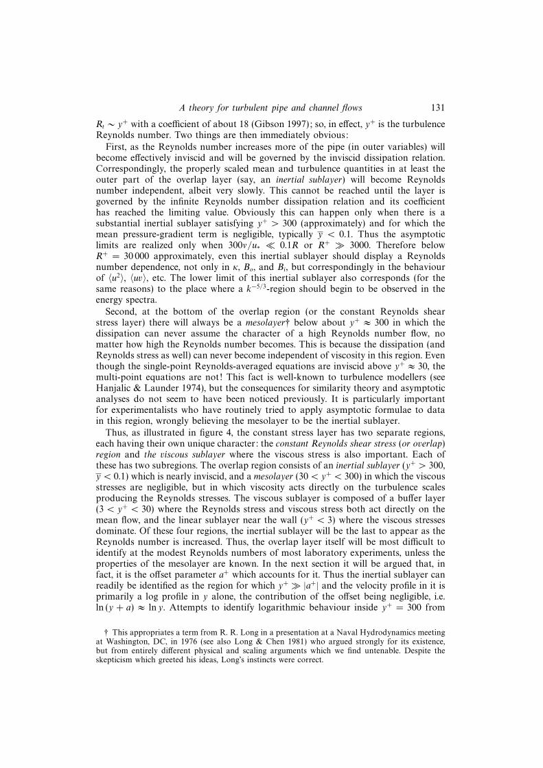
Rt ∼ y+ with a coefficient of about 18 (Gibson 1997); so, in effect, y+ is the turbulenceReynolds number. Two things are then immediately obvious:
First, as the Reynolds number increases more of the pipe (in outer variables) willbecome effectively inviscid and will be governed by the inviscid dissipation relation.Correspondingly, the properly scaled mean and turbulence quantities in at least theouter part of the overlap layer (say, an inertial sublayer) will become Reynoldsnumber independent, albeit very slowly. This cannot be reached until the layer isgoverned by the infinite Reynolds number dissipation relation and its coefficienthas reached the limiting value. Obviously this can happen only when there is asubstantial inertial sublayer satisfying y+ > 300 (approximately) and for which themean pressure-gradient term is negligible, typically y < 0.1. Thus the asymptoticlimits are realized only when 300ν/u∗ � 0.1R or R+ � 3000. Therefore belowR+ = 30 000 approximately, even this inertial sublayer should display a Reynoldsnumber dependence, not only in κ, Bo, and Bi, but correspondingly in the behaviourof 〈u2〉, 〈uv〉, etc. The lower limit of this inertial sublayer also corresponds (for thesame reasons) to the place where a k−5/3-region should begin to be observed in theenergy spectra.
Second, at the bottom of the overlap region (or the constant Reynolds shearstress layer) there will always be a mesolayer† below about y+ ≈ 300 in which thedissipation can never assume the character of a high Reynolds number flow, nomatter how high the Reynolds number becomes. This is because the dissipation (andReynolds stress as well) can never become independent of viscosity in this region. Eventhough the single-point Reynolds-averaged equations are inviscid above y+ ≈ 30, themulti-point equations are not! This fact is well-known to turbulence modellers (seeHanjalic & Launder 1974), but the consequences for similarity theory and asymptoticanalyses do not seem to have been noticed previously. It is particularly importantfor experimentalists who have routinely tried to apply asymptotic formulae to datain this region, wrongly believing the mesolayer to be the inertial sublayer.
Thus, as illustrated in figure 4, the constant stress layer has two separate regions,each having their own unique character: the constant Reynolds shear stress (or overlap)region and the viscous sublayer where the viscous stress is also important. Each ofthese has two subregions. The overlap region consists of an inertial sublayer (y+ > 300,y < 0.1) which is nearly inviscid, and a mesolayer (30 < y+ < 300) in which the viscousstresses are negligible, but in which viscosity acts directly on the turbulence scalesproducing the Reynolds stresses. The viscous sublayer is composed of a buffer layer(3 < y+ < 30) where the Reynolds stress and viscous stress both act directly on themean flow, and the linear sublayer near the wall (y+ < 3) where the viscous stressesdominate. Of these four regions, the inertial sublayer will be the last to appear as theReynolds number is increased. Thus, the overlap layer itself will be most difficult toidentify at the modest Reynolds numbers of most laboratory experiments, unless theproperties of the mesolayer are known. In the next section it will be argued that, infact, it is the offset parameter a+ which accounts for it. Thus the inertial sublayer canreadily be identified as the region for which y+ � |a+| and the velocity profile in it isprimarily a log profile in y alone, the contribution of the offset being negligible, i.e.ln (y + a) ≈ ln y. Attempts to identify logarithmic behaviour inside y+ = 300 from
† This appropriates a term from R. R. Long in a presentation at a Naval Hydrodynamics meetingat Washington, DC, in 1976 (see also Long & Chen 1981) who argued strongly for its existence,but from entirely different physical and scaling arguments which we find untenable. Despite theskepticism which greeted his ideas, Long’s instincts were correct.

132 M. Wosnik, L. Castillo and W. K. George
Uc
Pipe or channel centreline
Turbulent core
y+ y–
R+ 1
Outerequations
0.1R+ 0.1
Innerequations
Inertial sublayer
Meso layer
Buffer layer
Linear sublayer
Overlap region
Viscoussublayer
30
3
300
Figure 4. Schematic showing various regions and layers of pipe and channel flows.
straight lines on semi-log plots of u+ versus y+ are of little use if the theory presentedherein is correct because of the presence of a. They will, of course, always succeed asa local approximation, but coefficients so determined will be incapable of extensionto higher values of y+ as the Reynolds number is increased. And this is indeed thehistory of attempts to identify the log layer and its parameters from such data.
8. A mesolayer interpretation of a+
As noted in § 4 above, Squire (1948) was apparently the first to notice the need forthe offset coordinate y+ + a+. The basis of his argument was that the mixing lengthcould not be taken as proportional to y alone, since the physics incorporated in it couldnot account for the thickness of the viscous sublayer. Although the overlap analysispresented here depends on different closure assumptions, the argument concerninginvariance to coordinate origin presented earlier is not much different, in principle atleast. The preceding section argues for the existence of a mesolayer below the usualinertial layer in which the well-known scale separation of the energy and dissipativeeddies cannot exist. The purpose of this section is to show how these last two ideasare related.
The overlap solution of equation (4.19) can be expanded for values of y+ � |a+|:U
u∗= fi(y
+, R+) =1
κ
{[ln y+ + κBi] +
a+
y+− 1
2
a+2
y+2+
1
3
a+3
y+3+ · · ·
}. (8.1)

A theory for turbulent pipe and channel flows 133
For y+ � 2|a+|, this can be approximated by the first three terms as
U
u∗≈ 1
κln y+ + Bi +
a+
κy+. (8.2)
An equivalent expansion in outer variables is given by
U −Uc
u∗≈ 1
κln y + Bo +
a
κy. (8.3)
Equations (8.2) and (8.3) are useful for three reasons: First, they are an excellentapproximation to the overlap solutions for values of y+ > 2|a+| (or y > 2|a|). Second,they are easier to incorporate into a composite solution which includes the viscoussublayer than is the overlap solution itself since they do not have the singularity aty+ = −a+ (cf. GC). Third, the inner variable version can be shown to offer usefulinsight into the role of the parameter a+ as accounting for the mesolayer.
In the overlap region the turbulence energy balance reduces to production equalsdissipation, i.e. in inner variables, P+ ≈ ε+. This is exactly true in the limit ofinfinite Reynolds number, and approximately true at finite Reynolds numbers for30 < y+ < 0.1R+. It follows immediately by substitution of the overlap solutions forvelocity, Reynolds stress and dissipation for P+ and ε+ that
P+ =Bi12
κ(y+ + a+)= ε+ =
Ei
(y+ + a+). (8.4)
It is clear that the offset a+ must be the same for both velocity and dissipation, asassumed earlier. Hence Ei = Bi12/κ → 1/κ, at least in the limit as R+ → ∞ sinceBi12 → 1.
Therefore, in this limit the dissipation and velocity derivative profiles are identical(as noted earlier) and equal to the derivative of equation (4.19) with respect to y+, i.e.
ε+ =1
κ(y+ + a+)= ε+
o fT (y+), (8.5)
where
ε+o ≡ 1
κy+(8.6)
and
fT ≡[1 +
a+
y+
]−1
≈ 1− a+
y+, (8.7)
where the higher terms in the expansion in a+ have been neglected. This is iden-tical to the form used by many turbulence modellers for wall-bounded flows (cf.Reynolds 1976; Hanjalic & Launder 1974) to account empirically for the changein the character of the dissipation near the wall since Rt ≈ 18y+ as noted earlier.Thus the interpretation of a+ as a mesolayer parameter is obvious since it, in effect,modifies the dissipation (and hence the velocity profile) near the wall. The suggestedvalue of a+ = −8 accomplishes this.
A similar form of fT is obtained if the power law profile of GC for the boundarylayer is expanded, even though the form of εo is different. Interestingly, if the order ofargument is reversed and any of the simple dissipation models (e.g. Reynolds 1976)are used to deduce the mesolayer contribution to the velocity profile for the boundary
layer, they produce a y+−1additive instead of the y+γ−1
required. Obviously these

134 M. Wosnik, L. Castillo and W. K. George
0.020
0.015
0.010
0.005
Theory, κ∞= 1/0.447
0 2 4 6(×105)
1/κ –
1/κ
∞
R+
Figure 5. Variation of 1/κ− 1/κ∞ with R+, κ∞ = 0.447.
simple turbulence models, as currently posed, are consistent with the theory developedherein only for homogeneous flows, although the difference is slight.
Note that the common practice of choosing the model constants in equation (8.7)to produce a log profile at y+ ≈ 30 is clearly wrong if the proposed theory iscorrect, since this is the location where the mesolayer only begins. As noted in § 7,the mesolayer ends at y+ ≈ 300, and the inertial sublayer begins. It follows that a+
should be chosen to ‘turn off’ the low Reynolds number contribution at about thispoint (for increasing y+) and ‘turn on’ the ln y solution.
9. The superpipe velocity dataNow that the approximate region of validity of the overlap solution has been
established as 30 < y+ < 0.1R+ it is possible to test the theoretical profiles and theproposed layer model for the Reynolds number dependence. If they are correct, onlyan independent determination of either Bi or Bo is necessary to completely specifythe profile, the rest of the parameters having been determined from the friction data.Since the superpipe experiments have a substantial range satisfying the conditionsfor the existence of the inertial sublayer (300 < y+ < 0.1R+), it should be possible toestablish the value of Bi (or Bo) independent from the mesolayer. Also it should bepossible to determine whether the parameter a+ accounts for the mesolayer behaviour,at least for those data sets where data are available below y+ = 300.
For all of the data sets it appears that Bi = 6.5 is nearly optimal (at least forvalues of R+ > 850, the lowest available in this experiment), so that for the remainderof this paper it will be assumed that Bi = Bi∞. This value is close to the value of6.15 determined by Zagarola & Smits (1998a), who assumed κ fixed at 0.436. Sincethe difference, Bi∞ − Bo∞ = 8.45, was established from the friction data, it followsthat Bo∞ = −1.95. (Note, however, that the DNS channel data below suggest thatBo∞ = −2.1 and Bi∞ = 6.35 might be more appropriate, but the evidence is notconclusive yet.)
The constancy of Bi implies that it is Bo which shows all the Reynolds numberdependence of the difference given by equation (5.8). Figures 5 and 6 show thetheoretical variation of 1/κ and Bo with Reynolds number (equations (5.1) and (5.2)).Clearly both converge very slowly to their asymptotic values. This has far morerelative effect on Bo than it does on 1/κ, however, since Bo has achieved only 85%of its asymptotic value at R+ = 105. The observed variation of 1/κ and Bo and theconstancy of Bi can be contrasted with the boundary layer results of George et al.

A theory for turbulent pipe and channel flows 135
0.45
0.40
0.35
0.30
Theory, Βo,∞ = –1.95
0 2 4 6(×105)
B o –
Bo,
∞
R+
Figure 6. Variation of Bo − Bo,∞ with R+, Bo∞ = −1.95.
(1996) and GC in which Co, the outer coefficient, was nearly constant while the powerexponent γ and the inner coefficient Ci varied over the entire range of Reynoldsnumbers available.
Therefore the outer profile scaling will show more variation with Reynolds numberin the overlap region than the inner where only κ varies. This explains a great deal ofthe problems historically in establishing what Bo∞ is and in determining whether theouter scaling is correct. And it might also explain the conclusion of Zagarola & Smits(1998a) that a different scale for the outer flow is required, especially if attention isfocused on the overlap region instead of the core region of the flow.
Figures 7 and 8 show representative velocity profiles of the superpipe data at highand low Reynolds numbers, respectively. The profiles scaled in inner variables areshown in the upper plots, and the same data scaled in outer variables are shown in thelower plots. Also shown for each profile are the overlap solutions of equations (4.18)and (4.19) together with equations (5.7) and (5.8). The vertical lines on each profileshow the suggested bounds for the two sublayers of the overlap region; in particular,the mesolayer (30 < y+ < 300 or 30/R+ < y < 300/R+) and the inertial sublayer(300 < y+ < 0.1R+ or 300/R+ < y < 0.1). The limits vary with R+ for each profile.Note that for the highest Reynolds number plots the data were not measured closeenough to the wall to see any of the mesolayer; however, they do show clearly theinertial sublayer. For the lowest Reynolds numbers, enough of the near-wall regionwas resolved to clearly see the mesolayer, but the extent of the inertial sublayer waslimited or non-existent. The theoretical profiles were computed using the measuredvalue of R+ and assuming a+ = 0, −8, and −16 (or a = 0, −8/R+, and −16/R+). (Asnoted above, the value of Bo∞ = −1.95 is determined since Bi∞ has been chosen as6.5 and Bi∞ − Bo∞ = 8.45 from the friction data.) Therefore there are no adjustableparameters in the outer-scaled plot if a+ is determined from the inner. Thus theseouter profiles provide a completely independent test of the theory (and the data aswell).
The value of a+ = 0 corresponds to the inertial sublayer solution only, and asexpected describes the data well only in the range of 300 < y+ < 0.1R+. Theboundary layer value of a+ = −16 (from the power law) is clearly too large, butthen there is no reason to expect it to be the same since the homogeneous pipe andinhomogeneous boundary layer flows are fundamentally different, at least in the outerand overlap regions. The best fit to the DNS channel flow data (see below) abovey+ ≈ 30 is also a+ = −8. It is possible to fit the data to substantially lower values ofy+ by using different values of a+, but there appears to be no theoretical justification

136 M. Wosnik, L. Castillo and W. K. George
1
2
40
30
20
10
1010
102 103 104 105 106 107
Superpipe dataInertial sublayer (a+=0)Overlap eqn (4.19), a+=–8
R+ =25 228
R+ =76 096
R+ =216 030
R+ =528 556
Inertial sublayerMesolayer
y+=30 y+=300 y+=0.1R+
U+
U+ –5
U+ –10
U+ –15
y+
20
10
–10
10–4
0
–2010–3 10–110–2 10–0 10–1
y/R
Superpipe dataInertial sublayer (a+=0)Overlap eqn (4.18), a+=–8
Inertial sublayerMesolayer
R +=25 228
R +=76 096
R +=216 030
R +=528 556
300/R+30/R+
Udef
Udef –5
Udef –10
Udef –15
0.1
U/u
*U
– U
c/u
*
Figure 7. Inner and outer profiles at relatively high Reynolds number.
for doing so. Note that the Pitot tube used to make the pipe velocity measurementscould be as much as 2% percent too high at y+ = 30 because of the local turbulenceintensity there (since Umeas/U ≈ 1+[〈u2〉+〈v2〉+〈w2〉]/2U2). Additional positive errorsprobably arise when the probes are closest to the wall because of the asymmetry in the

A theory for turbulent pipe and channel flows 137
1
100 101 102 103
Superpipe dataInertial sublayer (a+=0)Overlap eqn (4.19), a+=–8
InertialsublayerMesolayer
y+=30 y+=300
2
30
20
10
0
–10105104
y+
U+
U+ –5
U+ –10
Overlap eqn (4.19), a+=–16
R+ =1091
R+ =3322
R+ =8486
0.1R+
0.1R+
0.1R+ No Inertial sublayer exits
100 101
Mesolayer
y+=30 y+=300
30
U+
U+ –5
U+ –10
R+ =1091
R+ =3322
R+ =8486
0.1R+
0.1R+
0.1R+
Superpipe dataInertial sublayer (a+=0)Overlap eqn (4.18), a+=–8
InertialsublayerMesolayer
20
Overlap eqn (4.18), a+=–16
R +=8486
30/R+
No inertial sublayer exists
300/R+30/R+
Udef –5
Udef
R +=3322
R +=1091
30/R+
y/R
10–110–2 10–0 10–1
–10
–5
0
5
10
15
Mesolayer
Mesolayer300/R+
Udef –5=(Uc–U)/u*
10–3
300/R+
Udef –10
U –
Uc/u
*U
/u*
Figure 8. Inner and outer profiles at relatively low Reynolds number.
streamline pattern around them. In spite of this, the agreement between experimentand theory over the entire overlap region is particularly gratifying since the velocitydata were only used to establish Bi and a+, the remaining parameters having beenentirely determined by the friction data.

138 M. Wosnik, L. Castillo and W. K. George
10
1101 102 103 104 105
Present results (a+=0)Present results (a+=–8)Present results (a+=–16)Zagarola & SmitsBarenblatt, Re =4×10⁴ to 4×10⁷
Classical theory, κ=0.41, B=5.2Kim (channel, DNS), R+=594Durst et al. (LDA)Zagarola & Smits
y+dU
+/d
y+
y+ = yu* /ν
Figure 9. Comparison of data and theories for y+du+/dy+ versus y+.
10. Comparison with other data and theoriesFigure 9 shows the profiles of y+dU+/dy+ computed from a number of sources,
including the LDA experiment of Durst, Jovanovic & Sender (1995) and the DNSdata discussed below. Also shown are a comparison of the present theoretical resultswith the classical theory and the recent contributions of Zagarola & Smits (1998a)and Barenblatt (1993). Only a single κ = 0.447 is used for the present theory since ininner variables the parameters are nearly constant, but the same three values of a+
(−16,−8, and 0) are shown. The present theory reduces to a constant in these variablesonly when a+ = 0. On the other hand for large values of y+, y+dU+/dy+ → 1/κ forall values of a+.
The data themselves are not very helpful, especially in the important region fromy+ = 30 to 100. The most that can be said from all the data taken together is thatthe value of a+ is bounded by these values. A case could be made that −16 is thebest choice if the Durst et al. data are used. On the other hand, the DNS channeldata discussed below would tend to indicate that zero might better.
There are two reasons why the data are problematical. First, the only reliable datain this region are from experiments or simulations in which the Reynolds numberis so low that it is impossible to distinguish an overlap region which is reasonablyindependent of the inner and outer layers. GC dealt with this problem for boundarylayers by using semi-empirical inner and outer profiles, then building a compositesolution so all the effects could be considered. Obtaining such a composite solutioncertainly should be a focus of future work. Second, as noted above, this is probably themost difficult region in which to measure accurately. The errors in measurement withvirtually every probe are larger than the differences between the theories which are beingcompared, especially for the higher Reynolds numbers. Clearly better experimentsand/or simulations at higher Reynolds numbers are necessary.
Figure 10 compares velocity profiles in the overlap region of the present theoreticalresult with the classical theory and the recent contributions of Zagarola & Smits(1998a) and Barenblatt (1993). As noted above there is little difference between the

A theory for turbulent pipe and channel flows 139
35
101 102 103 104 105
Present resultsZagarola & SmitsBarenblatt, Re =4×10⁴ to 4×10⁷
Classical theory, κ=0.41, B=5.2
U+ =
U/u
*
y+ = yu* /ν
30
25
20
15
10
Re (Barenblatt)
Re (Barenblatt)
Present results andZagarola & Smits almost
identical at high Re
Figure 10. Comparison of velocity profiles from various theories.
present results and that of Zagarola & Smits except below y+ < 300–500 for whichthe latter suggest that a power law region exists. Although it can certainly be arguedthat a power law fits their low Reynolds number data in this region, there is reason todoubt both the data and the matching procedure used to obtain the power law result.As noted above, measurements with Pitot tubes close to (or even on) the wall mightbe expected to be in error by the small amounts of interest here. Also, the matchingprocedure they employ depends on the existence of an outer-scale velocity differentfrom that used to obtain the log region. The outer scale they suggest, Uc − Um, isproportional to u∗ in the limit in which the matching is carried out, hence only a logprofile can result (cf. Appendix I of GC).
The family of curves due to Barenblatt can at most be argued to fit a region whichmoves to the right as the Reynolds number is increased. This is exactly what would beexpected if the power law form being fitted were not the right choice for an overlapregion, a conclusion consistent with the difficulties in this ‘theory’ in accounting forthe superpipe friction data as noted earlier.
11. Channel versus pipe flowAlthough both fully developed channel and pipe flows are homogeneous in the
stream-wise direction and both scale with u∗, there is no reason, in principle, to expectthe outer flow or overlap profiles of channel flow to be the same as for pipe flow.The former is planar and homogeneous in planes parallel to the surface, while thelatter is axially symmetric. The geometries are different, but the averaged equationsare nearly the same, differing only in the turbulence and viscous transport terms.
The inner regions of both flows have long been known to be quite close (seeMonin & Yaglom 1971). In fact, they must be exactly the same in the limit as theratio of the extent of the viscous sublayer to the pipe radius (or channel half-width)goes to zero. Therefore it is reasonable to hypothesize that the inner regions of bothflows be the same. Then the only differences between channel and pipe flows mustappear in the outer flow. If this is true, then all of the parameters governing the innerregion (including the overlap region in inner variables) must be the same for both

140 M. Wosnik, L. Castillo and W. K. George
25
20
15
10
5
0
–5
–10101 102 103
DNS data, Kim (1997)DNS data, Kim (1989)DNS data, Kim et al. (1987)Inertial sublayer (a+=0)Overlap eqn (4.19), a+=–8
y+
1
Mesolayer
0.1R+
0.1R+
0.1R+
y+=30
R+=180
R+=395
R+=595
U+
U +–5
U+–10
y+ = 300
20
15
10
5
0
–5
–1010–2 10–1 10–0
30/R+
30/R+
30/R+
Mesolayer
R +=395
R +=180
R +=595
300/R+
300/R+
(Uc–U )/u*
(Uc–U )/u*–5
(Uc–U )/u*–10
y/R
DNS data, Kim (1997)DNS data, Kim (1989)DNS data, Kim et al. (1987)Inertial sublayer (a+=0)Overlap eqn (4.18), a+=–8
2
Mesolayer
U –
Uc/u
*U
/u*
Figure 11. Channel flow DNS data of Kim et al. (1987), Kim (1989) and Kim (1997).
pipe and channel flows. In particular, the parameters κ and Bi must be the same, aswell as their dependence on Reynolds number. Hence even the empirical constantsA and α must be identical. Only the parameter Bo and the scale constant Ds can bedifferent. Moreover, since equation (4.22) must be satisfied, the channel flow value

A theory for turbulent pipe and channel flows 141
of Bo can at most differ by an additive constant from the pipe flow value, since anyother difference would affect the Reynolds-number-dependent relation between κ andBi − Bo.
Figure 11 shows the mean velocity profile data from the channel flow simulationsof Kim, Moin & Moser (1987) and Kim (1989) at values of R+ = 180 and 395, whereR in this case is taken to mean the channel half-width. Also shown is the profilefrom data given to us by J. Kim 1997, at R+ = 595.† As before the profiles scaled ininner variables are presented in the upper figure, and the same data in outer variablesin the lower. By the criteria established earlier, there should be no region which isdescribed by a simple logarithmic profile alone without the mesolayer contribution,even at the highest Reynolds number. In fact, as is clear from the vertical lines on theplots, there should not even be a mesolayer region in the lowest Reynolds numberprofile (since 0.1R+ < 30).
Nonetheless, the theoretical overlap solution, equation (4.19), with exactly theparameter values used above for the superpipe data, fits all three sets of data ininner variables nicely over the very limited range 30 < y+ < 0.1R+. (In fact, thetheoretical curve appears to work well to values of y+ substantially closer to the wall,even though its use below y+ = 30 cannot be justified theoretically, at least not bythe arguments presented earlier.) It is not even necessary to adjust the scale factorDs which was chosen as unity, just as for the pipe data. This agreement is all themore remarkable because all of the constants have been obtained from the superpipeexperiment at much higher Reynolds number.
The theoretical outer velocity profile uses the pipe values for all constants exceptfor Bo∞ as noted above. Since Bo∞ is quite small for the channel flow, even smalluncertainties about its value have a relatively large effect on the outer profile. There-fore the approach taken here has been to first determine Bi∞ − Bo∞ from the channelfriction data, then use the value of Bi∞ from the superpipe (since they should bethe same as noted above) to determine Bo∞ for the channel. Thus the channel flowvelocity data scaled in outer variables provide a completely independent test of thetheory. Unlike the superpipe data, however, there is much less DNS data available soa sophisticated optimization is not possible. However, there is only a single parameterwhich needs to be determined. Note that the experimental channel flow data havebeen avoided entirely because of uncertainties about the shear stress (see Kim et al.1987).
The best overall fit to the friction data, Uc/u∗, is achieved by choosing Bi∞ −Bo∞ =7.0 with the relative errors being 0.18%, 0.57%, and 1.2% for the Reynolds numbersof 595, 395, and 180 respectively. It follows that Bo∞ = −0.5.
As shown in the lower plot of figure (11), equation (4.18) provides a reasonable fitto the higher Reynolds number profiles over the same region as for the inner scaling.The fit is especially impressive since there has been no effort to optimize the fit tothe velocity profile data. (Recall that all constants but one were determined by thesuperpipe and the remaining one was chosen from the friction data!) A near perfectfit (not shown) to the two higher Reynolds number profiles can be achieved, however,by using Bo∞ = −0.65. This will increase the relative error in the friction estimates to0.089%, 1.3%, and 2.0%, respectively, if Bi is maintained at 6.5. On the other hand,if the value of Bi∞ is reduced to 6.35, then both the better friction prediction andthe better outer profile fits can be maintained simultaneously (since Bi inf − Bo∞ = 7.0
† The authors are very grateful to Professor Kim for making these data available to us. It hassince been published as Moser, Kim & Mansour (1999).
142 M. Wosnik, L. Castillo and W. K. George
is maintained), but with little relative change to the inner profile. Note that such avalue for Bi would be closer to the value of 6.15 suggested by Zagarola & Smits(1998a). The authors have resisted the urge to re-analyse the pipe flow data untilhigher Reynolds number DNS data confirm the need to do so, but it is clear that theonly other effect would be to change the pipe flow value of Bo∞ from −1.95 to −2.1which would hardly be noticeable in the plots.
All of the errors between the calculated and DNS values of Uc/u∗ are withinthe uncertainty of the DNS data itself which is estimated at 1–2%. The reason forthe larger discrepancy between the lower Reynolds number profiles is probablythat the theory is simply being stretched to Reynolds numbers below where it canreasonably be expected to apply. It is clear that the value of Bo∞ is substantially lowerfor the channel than for the pipe, but this was expected since, as noted above, thedifferences between the two flows should show up only in the outer flow.
The success of the theory developed herein in accounting for the channel flowdata using the pipe flow constants should give considerable confidence in the entiretheoretical approach. Moreover, it provides an independent confirmation of thevalues of the constants and the empirical function utilized for the Reynolds numberdependence.
12. Summary and conclusionsThe asymptotic invariance principle and the deductions from near asymptotics,
together with the recognition of the existence of a mesolayer, have provided anexcellent description of the mean velocity and skin friction data from fully developedchannel and pipe flows over more than three and a half decades in Reynolds number.Specifically the theory describes the velocity profile in the region 30 < y+ < 0.1R+ (or30/R+ < y < 0.1) for the superpipe experiment (850 < R+ < 530 000) and the lowReynolds number DNS data as well (R+ = 180, 395 and 595). Of the five parametersneeded to describe the flow, four could be determined only from the friction dataalone. Three of these (κ∞ = 0.447, A = −0.67 and α = 0.44) probably apply toany streamwise homogeneous wall-bounded flow. The difference parameter whichappears in the friction law, Bi∞−Bo∞, is different for pipes and channels (even thoughBi∞ is the same). From the superpipe experiment, Bi∞ − Bo∞ = 8.45, while from theDNS channel data it was estimated to be 7.0. Both pipe and channel data sets wereconsistent with constant values of Bi ≈ Bi∞ = 6.5 and a+ = −8. It follows that theouter parameter Bo∞ = −1.95 for the pipe flow, and −0.5 for the channel flow. Acase can also be made that the limiting values of Bo∞ should be −2.1 and −0.65corresponding to Bi∞ = 6.35, but a final decision can probably not be made untilhigher Reynolds number DNS data become available.
Unlike the boundary layer, where both Reynolds number effects and the mesolayerwere of equal importance in understanding the data, for pipe and channel flows theReynolds number dependence was found to be slight. In fact, only Bo shows significantvariation over the range of the data, and then only about 5%. The variation of thevon Karman parameter, κ, was only about 1%; and both Bi and a+ were constant towithin the accuracy of the data.
On the other hand, the mesolayer concept (and a+ in particular) proved crucial inunderstanding where the theory applied and in understanding why previous attemptsto verify the log law were less than totally satisfactory. In particular, the overlap meanvelocity profile was found to not be a simple logarithm in y, but instead a logarithmin y + a. The most important consequence of this is that attempts to establish ln y
A theory for turbulent pipe and channel flows 143
behaviour using velocity profile data inside y+ = 300 are doomed to failure and theresults misleading unless the mesolayer (and a in particular) are explicitly accountedfor. This, of course, explains much of the confusion in the literature about preciselywhat the log parameters were and where the theory applied – not only was the wrongprofile being used, but it was being applied to the wrong region.
It should be noted that for their boundary layer data analysis, George et al. (1996)and GC used a procedure which was the reverse of that used here. There a series ofcareful attempts was first made to obtain directly the variation of the parameters fromthe velocity profiles, then the friction law was inferred and shown to be in agreementwith direct measurements. The fact that the procedure followed here has been equallysuccessful lends credibility to both analyses, especially in view of the importance ofthe subtle difference between the friction law proposed here and a simple log lawwith constant coefficients.
There are a number of interesting questions which remain. One of these is whetherthe mesolayer parameter a+ is indeed constant, as it appears it might be. This willrequire accurate measurements of the velocity profile near y+ = 30 at considerablyhigher Reynolds numbers than has been possible to date. Note that the problem isnot with the overall flow Reynolds number (which in the superpipe was certainlyadequate), but with the inability to resolve the flow near the wall at the higherReynolds numbers due to probe size limitations. An obvious solution is a bigger pipeso less absolute resolution is required at a given Reynolds number – a mega-pipeperhaps (or a mighty duct!).
Another question arises from the Reynolds number dependence itself which isnearly negligible for channel and pipe, but crucial for boundary layer flows. Is thisa subtle consequence of the homogeneity of the former and inhomogeneity of thelatter, or is it simply a reflection of the differing inner and outer velocity scales forthe boundary layer with the consequent Reynolds number dependence? Or are thesethe same thing? Or is the boundary layer’s dependence a residual of the dependenceon upstream conditions?
Then there is the fact that the parameter, α, which accounts for the Reynoldsnumber dependence is nearly the same as for the boundary layer, and tantalizinglyclose to κ∞ and the boundary layer value of 1/(γ∞Co∞). The possible universality ofthese is particularly interesting, especially given the agreement between theory andexperiment for both the homogeneous and inhomogeneous flows. A consequence ofthis is that the dissipation profiles for the pipe and the infinite Reynolds numberboundary layer are nearly identical throughout the overlap region, even though theydiffer substantially for the finite Reynolds numbers of experiments. And, of course,this raises the question for the functions H (for the pipe and channel) and h (forthe boundary layer) which contain the essential Reynolds number dependence of theflow: Can they (or alternatives) be derived directly from the underlying physics of theflow, perhaps through symmetry considerations of the turbulence dissipative scales orfrom the multi-point equations?
In conclusion, unlike the classical boundary layer theory which was shown byGC to be fundamentally flawed, the same approach has been able to show that theclassical theory for pipe and channel flows is really pretty good. The present analysishas, from purely deductive reasoning using the Reynolds-averaged Navier–Stokesequations, been able to identify why the classical results were not totally successful,and was able to account for recent DNS, LDA and superpipe observations. Thus itwould seem that the Navier–Stokes equations indeed apply to turbulence, hardly anovel idea to most, but reassuring nonetheless.
144 M. Wosnik, L. Castillo and W. K. George
The authors are particularly grateful to J. Kim, L. Smits, and M. Zagarola formaking their work available to us, and also to M. Oberlack for helping us understandthe need for the origin shift in the overlap analysis. The invitation to participatein the Disquisitiones Mechanicae 1996 at the University of Illinois, Department ofTheoretical and Applied Mechanics did much to focus our thinking and move thiswork forward. The efforts of Professors R. Adrian, S. Balachandar, R. Moser andespecially H. Aref to organize and host it are greatly appreciated.
REFERENCES
Barenblatt, G. I. 1993 Scaling laws for fully developed shear flow. Part 1. Basic hypotheses andanalysis. J. Fluid Mech. 248, 513–520.
Barenblatt, G. I. 1996 Scaling, Self-Similarity, and Intermediate Asymptotics. Cambridge UniversityPress.
Barenblatt, G. I. & Chorin, A. J. 1998 Scaling of the intermediate region in wall-boundedturbulence: The power law. Phys. Fluids 10, 1043–1044.
Barenblatt, G. I., Chorin, A. J. & Prostokishin, V. M. 1997 Scaling laws for fully developed flowin pipes. Appl. Mech. Rev. 50, 413–429.
Barenblatt, G. I. & Prostokishin, V. M. 1993 Scaling laws for fully developed shear flow. Part 2.Processing of experimental data. J. Fluid Mech. 248, 521–529.
Bush, W. B. & Fendell. F. E. 1974 Asymptotic analysis of turbulent boundary layer and channelflow. J. Fluid Mech. 56, 657–681.
Cole, J. D. & Kevorkian, J. 1981 Perturbation Methods in Applied Mathematis. Springer.
Duncan, W. J., Thom, A. S. & Young, A. D. 1970 Mechanics of Fluids, 2nd edn. Elsevier.
Durst, F., Jovanovic, J. & Sender, J. 1995 LDA measurement in the near-wall region of a turbulentpipe flow. J. Fluid Mech. 295, 305–335.
Frisch, U. 1995 Turbulence. Cambridge University Press.
Gad-el-Hak, M. & Bandyopadhyay, P. R. 1994 Reynolds number effects in wall-bounded flows.Appl. Mech. Rev. 47, 307–365.
George, W. K. 1988 Another look at the log (or is it a power law?) velocity profile for a zero-pressuregradient boundary layer. Bull. Am. Phys. Soc. 33 no. 10, 2301.
George, W. K. 1990 Another look at the log (or is it a power law?) velocity profile for a zero-pressuregradient boundary layer 3rd Joint ASME/ASCE Mech. Conf. La Jolla, CA, July 9–12.
George, W. K. 1995 Some new ideas for similarity of turbulent shear flows. In Proc. ICHMT Symp.on Turbulence, Heat and Mass Transfer, Lisbon, Portugal (1994) (ed. K. Hanjalic & J. C. F.Pereira). Elsevier.
George, W. K. & Castillo, L. 1993 Boundary layers with pressure gradient: Another look at theequilibrium boundary layer. In Near Wall Turbulent Flows (ed. R. M. C. So), pp. 901–910.Elsevier.
George, W. K. & Castillo, L. 1997 Zero-pressure-gradient turbulent boundary layer. Appl. Mech.Rev. 50, 689–729 (referred to herein as GC).
George, W. K., Castillo, L. & Knecht, P. 1996 The zero pressure-gradient turbulent boundarylayer. Tech. Rep. TRL-153. Turbulence Research Laboratory, University at Buffalo.
George, W. K., Castillo, L. &Wosnik, M. 1997 A theory for turbulent pipe and channel flows. Tech.Rep. 872. Theoretical and Applied Mechanics, University of Illinois at Urbana-Champaign.
George, W. K., Knecht, P. & Castillo, L. 1992 The zero pressure-gradient boundary layer revisited.13th Symposium on Turbulence, Rolla, MO.
Hanjalic, K. & Launder, B. E. 1974 Contribution towards a Reynolds stress closure for low-Reynolds number turbulece. Rep. HTS/74/24. Imperial College.
Kim, J. 1989 On the structure of pressure fluctuations in simulated turbulent channel flow. J. FluidMech. 205, 421–451.
Kim, J., Moin, P. & Moser, R. T. 1987 Turbulence statistics in fully developed channel flow at lowreynolds number. J. Fluid Mech. 177, 133–166.
Long, R. R. & Chen, T.-C. 1981 Experimental evidence for the existence of the ‘mesolayer’ inturbulent systems. J. Fluid Mech. 105, 19–59.

A theory for turbulent pipe and channel flows 145
Millikan, C. M. 1938 A critical discussion of turbulent flows in channels and circular tubes. InProc. 5th Intl Congress of Applied Mechanics, pp. 386–392. John Wiley and Sons.
Monin, A. S. & Yaglom, A. M. 1971 Statistical Fluid Mechanics. MIT Press.
Moser, R. T., Kim, J. & Mansour, N. N. 1999 Direct numerical simulation of turbulent channelflow up to Rer = 590. Phys. Fluids 11, 943–945.
Oberlack, M. 1997 Unified theory for symmetries in plane parallel turbulent shear flows. Manuscript163. Center for Turbulence Research, NASA Ames/Stanford University (also submitted toJ. Fluid Mech.).
Panton, R. 1990 Scaling turbulent wall layers. Trans. ASME: J. Fluids Engng 112, 425–432.
Perry, A. E. & Abell, C. J. 1975 Scaling laws for pipe-flow turbulence J. Fluid Mech. 67, 257.
Prandtl, L. 1932 Zur turbulenten Stroemung in Rohren und laengs Platten. Ergeb. Aerodyn. VersuchGoettingen IV. Lieferung, p. 18.
Reynolds, W. C. 1976 Computation of turbulent flows. Ann. Rev. Fluid Mech. 8, 183–208.
Smits, A. J. & Zagarola, M. V. 1998 Response to: Scaling of the intermediate region in wall-boundedturbulence: The power law (Phys. Fluids 10, 1043 (1998)). Phys. Fluids 10, 1045–1046.
Squire, H. B. 1948 Reconsideration of the theory of free turbulence. Phil. Mag. 39 (288), 1–20.
Stanton, T. E. & Pannell, J. R. 1914 Similarity of motion in relation to the surface friction offluids. Phil. Trans. R. Soc. Lond. A 214, 199.
Tennekes, H. 1968 Outline of a second-order theory of turbulent pipe flow. AIAA J. 6, 1735–1740.
Tennekes, H. & Lumley, J. L. 1972 A first Course in Turbulence. MIT Press.
Zagarola, M. V. 1996 Mean flow scaling in turbulent pipe flow. PhD thesis, Princeton University.
Zagarola, M. V. & Smits, A. J. 1998a Mean-flow scaling of turbulent pipe flow. J. Fluid Mech. 373,33–79.
Zagarola, M. V. & Smits, A. J. 1998b A new mean velocity scaling for turbulent boundary layers.In Proc. FEDSM’98, Washington DC. ASME.