Models of Turbulent Pipe Flow

Thesis by

Jean-Loup Bourguignon

In Partial Fulfillment of the Requirements

for the Degree of

Doctor of Philosophy

California Institute of Technology

Pasadena, California

2013

(Defended November 5, 2012)

ii

c© 2013

Jean-Loup Bourguignon

All Rights Reserved

iii

Acknowledgments

The guidance and support of Beverley McKeon, Dennice Gayme, Rashad Moarref, Ian Jacobi, and

Jeff LeHew are gratefully acknowledged. Xiaohua Wu kindly provided the DNS data for this thesis.

The comments and feedback of Ati Sharma and Joel Tropp on the third chapter were appreciated, as

well as their insightful advice. Support for this research provided by the Air Force Office of Scientific

Research under award # FA9550-09-1-0701 was greatly appreciated.

iv

Abstract

The physics of turbulent pipe flow was investigated via the use of two models based on simplified

versions of the Navier-Stokes equations. The first model was a streamwise-constant projection of

these equations, and was used to study the change in mean flow that occurs during transition to

turbulence. The second model was based on the analysis of the turbulent pipe flow resolvent and

provided a radial basis for the modal decomposition of turbulent pipe flow. The two models were

tested numerically and validated against experimental and numerical data.

Analysis of the streamwise-constant model showed that both non-normal and nonlinear effects

are required to capture the blunting of the velocity profile, which occurs during pipe flow transition.

The model generated flow fields characterized by the presence of high- and low-speed streaks, whose

distribution over the cross-section of the pipe was remarkably similar to the one observed in the

velocity field near the trailing edge of the puff structures present in pipe flow transition.

A modal decomposition of turbulent pipe flow, in the three spatial directions and in time, was

performed, and made possible by the significant reduction in data requirements achieved via the use

of compressive sampling and model-based radial basis functions. The application and efficiency of

compressive sampling in wall-bounded turbulence was demonstrated.

Approximately sparse representations of turbulent pipe flow by propagating waves with model-

based radial basis functions were derived. The basis functions, obtained by singular value decompo-

sition of the resolvent, captured the wall-normal coherence of the flow and provided a link between

the propagating waves and the governing equations, allowing for the identification of the dominant

mechanims sustaining the waves, as a function of their streamwise wavenumber.

Analysis of the resolvent showed that the long streamwise waves are amplified mainly via non-

normality effects, and are also constrained to be tall in the wall-normal direction, which decreases

the influence of viscous dissipation. The short streamwise waves were shown to be localized near the

critical-layer (defined as the wall-normal location where the convection velocity of the wave equals

the local mean velocity) and thus exhibit amplification with a large contribution from criticality.

The work in this thesis allows the reconciliation of the well-known results concerning optimal dis-

turbance amplification due to non-normal effects with recent resolvent analyses, which highlighted

the importance of criticality effects.

v

Contents

Acknowledgments iii

Abstract iv

List of Figures vii

List of Tables xiii

List of Symbols xv

1 Introduction 1

1.1 Motivation . . . . . . . . . . . . . . . . . . . . . . . . . . . . . . . . . . . . . . . . . 1

1.2 Analysis of the Navier-Stokes Equations Linearized Around the Laminar Profile . . . 2

1.3 Linear Analyses Based on the Turbulent Mean Velocity Profile . . . . . . . . . . . . 4

1.4 Nonlinear Studies in Wall-Bounded Turbulence . . . . . . . . . . . . . . . . . . . . . 5

1.5 Data-Based Analyses to Infer the Structure of Turbulence . . . . . . . . . . . . . . . 6

1.6 Thesis Outline . . . . . . . . . . . . . . . . . . . . . . . . . . . . . . . . . . . . . . . 8

2 A Streamwise-Constant Model of Turbulent Pipe Flow 10

2.1 Introduction . . . . . . . . . . . . . . . . . . . . . . . . . . . . . . . . . . . . . . . . . 10

2.2 Description of the Model and Numerical Methods . . . . . . . . . . . . . . . . . . . . 13

2.3 Simplified Streamwise-Constant Model with Deterministic Forcing . . . . . . . . . . 15

2.4 Stochastic Forcing of the Streamwise-Constant Model . . . . . . . . . . . . . . . . . 19

2.5 Summary . . . . . . . . . . . . . . . . . . . . . . . . . . . . . . . . . . . . . . . . . . 25

3 Efficient Representation of Wall-Bounded Turbulence Using Compressive Sam-

pling 26

3.1 Introduction . . . . . . . . . . . . . . . . . . . . . . . . . . . . . . . . . . . . . . . . . 26

3.2 Methodology . . . . . . . . . . . . . . . . . . . . . . . . . . . . . . . . . . . . . . . . 28

3.2.1 Synthetic Velocity Fields . . . . . . . . . . . . . . . . . . . . . . . . . . . . . 29

3.2.2 DNS Velocity Fields . . . . . . . . . . . . . . . . . . . . . . . . . . . . . . . . 32

vi

3.3 Results . . . . . . . . . . . . . . . . . . . . . . . . . . . . . . . . . . . . . . . . . . . . 34

3.3.1 Demonstration of Compressive Sampling Using Synthetic Velocity Fields . . . 34

3.3.2 Sparsity Check Based on Periodically Sampled DNS Data . . . . . . . . . . . 37

3.3.3 Frequency Analysis of Randomly Sampled DNS Data via Compressive Sampling 37

3.3.4 Comparison with Periodic Sampling . . . . . . . . . . . . . . . . . . . . . . . 47

3.4 Summary . . . . . . . . . . . . . . . . . . . . . . . . . . . . . . . . . . . . . . . . . . 49

4 Sparse Representation of Turbulent Pipe Flow by Propagating Waves and a

Model-Based Radial Basis 52

4.1 Introduction . . . . . . . . . . . . . . . . . . . . . . . . . . . . . . . . . . . . . . . . . 52

4.2 Methodology . . . . . . . . . . . . . . . . . . . . . . . . . . . . . . . . . . . . . . . . 58

4.2.1 Decomposition in the Streamwise and Azimuthal Directions . . . . . . . . . . 60

4.2.2 Decomposition in Time . . . . . . . . . . . . . . . . . . . . . . . . . . . . . . 60

4.2.3 Decomposition in the Radial Direction . . . . . . . . . . . . . . . . . . . . . . 62

4.2.4 Proper Orthogonal Decomposition . . . . . . . . . . . . . . . . . . . . . . . . 64

4.3 Results . . . . . . . . . . . . . . . . . . . . . . . . . . . . . . . . . . . . . . . . . . . . 65

4.3.1 Two-dimensional Fourier Modes (k,n) . . . . . . . . . . . . . . . . . . . . . . 65

4.3.2 Fourier Modes (k,n,uc) . . . . . . . . . . . . . . . . . . . . . . . . . . . . . . 68

4.3.3 Streamwise Singular Modes (k,n,uc,q) . . . . . . . . . . . . . . . . . . . . . 69

4.3.4 Comparison with Proper Orthogonal Decomposition . . . . . . . . . . . . . . 75

4.4 Discussion . . . . . . . . . . . . . . . . . . . . . . . . . . . . . . . . . . . . . . . . . . 78

4.4.1 Componentwise Form of the Input-Output Relationship . . . . . . . . . . . . 78

4.4.2 Influence of Non-Normality on Disturbance Amplification . . . . . . . . . . . 82

4.4.3 Influence of Criticality on Disturbance Amplification for High k Modes . . . 85

4.4.4 Implications of the Present Study on Analyses on Criticality and Non-Normality 90

4.5 Summary . . . . . . . . . . . . . . . . . . . . . . . . . . . . . . . . . . . . . . . . . . 93

5 Conclusion 95

A Matlab code used to solve the convex optimization problem 97

Bibliography 97

vii

List of Figures

2.1 The coordinate system used to project the Navier-Stokes equations. . . . . . . . . . . 14

2.2 (a) Streamfunctions Ψ1,a−c(r) and (b) corresponding velocity profiles u0(r) for Ψ1,a(r) =

0.033(r − 3r3 + 2r4) (thin solid), Ψ1,b(r) = 0.7(r − 3r3 + 2r4)2 (dashed), Ψ1,c(r) =

14(r−3r3+2r4)3 (dash-dot) and experimental velocity profile of den Toonder & Nieuw-

stadt (1997) at Re = 24, 600 (thick solid). . . . . . . . . . . . . . . . . . . . . . . . . 17

2.3 Model output for deterministic forcing: (a) contours of the streamfunction Ψ = 0.033 (r−

3r3+2r4) sin θ, (b) vector plot of the corresponding in-plane velocities, and (c) contours

of the resulting axial velocity field. . . . . . . . . . . . . . . . . . . . . . . . . . . . . 19

2.4 Contours of the axial velocity induced by the streamfunction Ψ6(r, θ) = (r4 − 2r5 +

r6) sin(6θ), the light and dark filled contours correspond to regions of the flow respec-

tively faster and slower than laminar. . . . . . . . . . . . . . . . . . . . . . . . . . . . 20

2.5 Time traces of the centerline velocity from three different simulations respectively at

Re = 2, 200 with 0.0005 and 0.002 rms noise levels (a), (c) and at Re = 10, 000 with

0.002 rms noise level (b). The resolution in the radial direction is N = 48. (d) Zoom

on the time interval during which the samples of figure 2.6 are taken. The vertical lines

indicate the sampling instants. . . . . . . . . . . . . . . . . . . . . . . . . . . . . . . . 21

2.6 Contours of the axial velocity, subfigures (a) to (c), and of the swirling strength for the

in-plane velocities, subfigures (d) to (f), computed respectively at τ = 1620, τ = 1700,

and τ = 1740 dimensionless time units. . . . . . . . . . . . . . . . . . . . . . . . . . . 22

2.7 Diagram detailing the different stages of the QSSP. The dashed lines represent unmod-

eled effects. . . . . . . . . . . . . . . . . . . . . . . . . . . . . . . . . . . . . . . . . . 24

3.1 Schematic of pipe geometry and nomenclature (McKeon & Sharma, 2010). . . . . . . 29

3.2 Frequency range resolved by the periodically sampled DNS data (delimited by the

two horizontal dashed lines) compared to the empirical upper and lower bounds on the

DNS frequency content (solid lines) as a function of the streamwise wavenumber k. The

shaded area shows the time-resolved streamwise wavenumber range for the available

data. . . . . . . . . . . . . . . . . . . . . . . . . . . . . . . . . . . . . . . . . . . . . . 33

viii

3.3 Frequency spectrum premultiplied by r as a function of the wall-normal distance y, for

the large-scale mode (k, n) = (1, 10), with the 8 input frequencies reported on table 3.1,

sampled during 100 (a) and 25 (b) dimensionless time units. The distorted contours

(b) indicate that the sparsity relationship is not satisfied. . . . . . . . . . . . . . . . . 35

3.4 Wall-normal profile of the magnitude (a) and phase (b) for the first three most energetic

modes (k, n) = (0.21,−2) (dotted), (k, n) = (0.42, 3) (dashed), and (k, n) = (0.21, 2)

(solid) of the periodically sampled DNS flow field. . . . . . . . . . . . . . . . . . . . . 38

3.5 Representative frequency spectrum corresponding to the 2D Fourier mode (k, n) =

(0.42, 5) as a function of the wall-normal distance, with the empirical upper and lower

bounds on frequency, corresponding to convection velocities equal to the centerline

velocity and 10 times the friction velocity, demarcated by the two vertical lines. . . . 39

3.6 The 50 DNS sampling time instants randomly distributed over 100 dimensionless time

units based on the radius and bulk velocity. The last sampling time instant is at

τ = 96.57. . . . . . . . . . . . . . . . . . . . . . . . . . . . . . . . . . . . . . . . . . . . 39

3.7 Power spectral density over the frequency range f ∈ [0, 0.1] as a function of the wall-

normal distance (a),(c) and integrated in the wall-normal direction (b),(d) for the 2D

Fourier mode (k, n) = (0.21, 2) from the randomly sampled DNS. The top and bottom

rows correspond to a local minimization with respectively 400 and 800 optimization

frequencies. The dots (b),(d) indicate the sparse frequencies. . . . . . . . . . . . . . . 41

3.8 Wall-normal profiles of the Fourier modes (k, n, ω) = (0.21, 2, 2πf) from the randomly

sampled DNS, for the different dominant frequencies, compared to the time average of

the original and reconstructed signals computed using the local (a) and global (b) mini-

mizations with 400 optimization frequencies, and the local (c) and global (d) minimiza-

tions with 800 optimization frequencies. The maximum frequency for the optimization

is 1 in both cases. . . . . . . . . . . . . . . . . . . . . . . . . . . . . . . . . . . . . . . 42

3.9 Power spectral density for the 2D Fourier mode (k, n) = (0.21, 2) from the randomly

sampled DNS obtained via optimal compressive sampling. . . . . . . . . . . . . . . . . 43

3.10 Contours of the real part of the 2D Fourier mode (k, n) = (0.21, 2) from the randomly

sampled DNS, as a function of the wall-normal distance and time, with all the frequen-

cies included (a) and with only three dominant frequencies recovered from compressive

sampling included (b). . . . . . . . . . . . . . . . . . . . . . . . . . . . . . . . . . . . . 44

3.11 Contours of the real part of the 2D Fourier modes (k, n) = (1.05, 2) (a) and (k, n) =

(3.14, 4) (c) from the randomly sampled DNS as a function of the wall-normal distance

and time. Wall-normal profiles of the Fourier modes (k, n, ω) = (1.05, 2, 2πf) (b) and

(k, n, ω) = (3.14, 4, 2πf) (d) for the different sparse frequencies compared to the time

average of the original and reconstructed signals. . . . . . . . . . . . . . . . . . . . . . 45

ix

3.12 (a) Time-averaged power spectral density in the wall-normal direction for the 2D

Fourier mode (k, n) = (3.14, 4) from the randomly sampled DNS. (b) Contours of

the real part of the 2D Fourier mode (k, n) = (3.14, 4) low-pass filtered and (c) high-

pass filtered showing the two different types of uniform momentum zones present in

the wall-normal direction. . . . . . . . . . . . . . . . . . . . . . . . . . . . . . . . . . . 46

3.13 Frequency content of the 2D Fourier modes as a function of the streamwise wavenumber

for various azimuthal wavenumbers (a). The two solid lines indicate the upper and lower

empirical bounds on the frequency content and the dashed line shows the streamwise

wavenumber corresponding to the near-wall type modes. The shaded areas highlight the

dynamically significant bandwidth and streamwise wavenumber range at Re = 24, 580

(a) and extrapolated to Re = 300, 000 (b). . . . . . . . . . . . . . . . . . . . . . . . . . 47

3.14 Comparison between the time-averaged wall-normal profile of the 2D Fourier mode

(k, n) = (0.21, 2) from the randomly sampled DNS and its two sparse frequencies

obtained using compressive sampling with 14 and 50 snapshots. . . . . . . . . . . . . . 49

3.15 Power spectral density of a superposition of three Fourier modes with unit magnitude

and frequencies f = 0.035, 0.052, 0.087 sampled 50 times during 100 time units com-

puted using (a) periodic sampling with FFT, and (b) compressive sampling with a

frequency increment of df = 0.01 and (c) df = 0.001. . . . . . . . . . . . . . . . . . . . 50

4.1 The 50 DNS sampling time instants randomly distributed over 100 dimensionless time

units based on the radius and bulk velocity. The last sampling time instant is at t = 96.57. 59

4.2 Schematic of pipe geometry and nomenclature. . . . . . . . . . . . . . . . . . . . . . 60

4.3 Block diagram representing the decomposition of fully developed turbulent pipe flow

as a sum of propagating waves. . . . . . . . . . . . . . . . . . . . . . . . . . . . . . . . 61

4.4 Comparison of the first (solid), second (dotted), and tenth (dashed) singular mode

profiles of the streamwise velocity component before (black) and after (gray) applying

the QR decomposition for the set of parameters (0.21, 2, 0.83). For the first two modes,

the profiles before and after QR decomposition are identical to plotting accuracy. . . . 64

4.5 Convergence of the turbulence intensities and kinetic energy as a function of the number

of 2D Fourier modes for one representative DNS snapshot. . . . . . . . . . . . . . . . 66

4.6 Time average wall-normal profile of the 2D Fourier mode (k, n) = (0.21, 2) compared

to the reconstructed profile using only the three dominant frequencies. The profiles of

the Fourier modes (0.21, 2, uc) at the three dominant frequencies corresponding to the

convection velocities uc = 0.71, 0.83, 0.95 are also shown for comparison. . . . . . . . 67

x

4.7 Contour plots of streamwise velocity fluctuations at θ = 0 for the DNS flow field Fourier

filtered in the streamwise direction (a) and the Fourier series approximation with 51

(k,n) modes capturing 20% of the streamwise turbulence intensity (b). . . . . . . . . 67

4.8 Contours of the real part of the 2D Fourier mode (k, n) = (0.21, 2) as a function of the

wall-normal distance and time with all the frequencies included (a) and with only the

three dominant frequencies included (b). The contours are obtained by interpolation

between the randomly sampled velocity fields, and plotted at θ = 0 and x = 0. . . . . 69

4.9 Contours of the streamwise velocity fluctuations in the streamwise and wall-normal

directions at two different time instants separated by half a period of the longest struc-

tures or about 14.3 dimensionless time units. The velocity fields from top to bottom are

reconstructed based on a superposition of respectively the top 2, 4, and 16 dominant

(k,n) wavenumber pairs with all the sparse frequencies included. The bottom velocity

field correspond to the DNS data Fourier filtered to remove the small scales. . . . . . 70

4.10 Wall-normal profiles for the magnitude (a),(c) and phase (in radians) (b),(d) of the sin-

gular modes (a),(b) (k, n, uc, q) = (0.21, 2, 0.83, 1) (dotted), (0.21, 2, 0.83, 2) (dashed),

and (0.21, 2, 0.83, 3) (solid); and (c),(d) (0.21, 2, 0.83, 4) (dotted), (0.21, 2, 0.83, 5) (dashed),

and (0.21, 2, 0.83, 6) (solid). Energy (e) and cumulative energy (f) captured as a func-

tion of the mode order and normalized by the DNS mode energy u′2 with (solid) and

without (dashed) QR orthonormalization. . . . . . . . . . . . . . . . . . . . . . . . . . 71

4.11 Wall-normal profiles for the magnitude (a) and phase (in radians) (b) of a superposition

of 1 (k, n, uc, q) = (0.21, 2, 0.83, 1), 3 (0.21, 2, 0.83, 1 : 3), and 6 (0.21, 2, 0.83, 1 : 6)

singular modes compared to the Fourier mode (k, n, uc) = (0.21, 2, 0.83) magnitude

and phase profiles. . . . . . . . . . . . . . . . . . . . . . . . . . . . . . . . . . . . . . . 72

4.12 Contours of the streamwise velocity fluctuations in a streamwise wall-normal plane for

the Fourier mode (k, n, uc) = (0.21, 2, 0.83) and its representation as a sum of respec-

tively 1 (k, n, uc, q) = (0.21, 2, 0.83, 1), 3 (0.21, 2, 0.83, 1 : 3), and 6 (0.21, 2, 0.83, 1 : 6)

singular modes (top to bottom). The horizontal dashed lines delimitate the region

where the Fourier mode and its representation are in phase. . . . . . . . . . . . . . . . 73

4.13 Average number of singular modes Nm required to capture 95% of u′2 as a function of

the streamwise wavenumber (a) and convection velocity (b) based on the decomposition

of 134 Fourier modes from the DNS turbulent pipe flow realization. . . . . . . . . . . 74

4.14 Wall-normal profile of the synthetic Fourier coefficient ck,n,ω(r) = (1−r)r4 (a). Number

of streamwise singular modes required to capture 99% of the analytic Fourier coefficient

energy at (k, n, uc) = (0.21, 2, 0.77) (solid) and (k, n, uc) = (1.47, 2, 0.77) (dashed) (b). 75

xi

4.15 Time-averaged wall-normal profile (a) and energy integrated in the wall-normal di-

rection as a function of time (b) of the 2D Fourier mode (k, n) = (0.21, 2) (dashed)

together with the first POD mode (solid, black) and the reconstructed 2D Fourier mode

based on three dominant frequencies (solid, grey). Note that the temporal Fourier ba-

sis functions are not orthogonal on the set of randomized sampling time instants such

that Parseval’s theorem does not apply, i.e., the time average profile differs from the

square root of the sum of the square of the three frequency components. (c) Phase of

the time-varying amplitude coefficient of the first POD mode compared to the phase of

the most energetic Fourier mode (k, n, uc) = (0.21, 2, 0.83). The phase of the Fourier

mode depends on the wall-normal distance but the phase speed is constant. The origin

of phase is chosen to match the POD mode. . . . . . . . . . . . . . . . . . . . . . . . . 76

4.16 Streamwise (a),(c) and azimuthal (b),(d) contributions to the forcing (top row) and

response (bottom row) energy, as a function of the streamwise wavenumber and singular

mode order, in the presence of mean shear and for n = 3, uc = 0.8. . . . . . . . . . . . 80

4.17 Cross-sectional contribution to the forcing energy for the first singular mode and with

n = 3. The preferential forcing direction switches from being mainly in the cross-

sectional plane at low k to being mainly streamwise at high k at a value of k around

4 – 5 corresponding to the streamwise length of the near-wall type structures (k = 4.3

corresponds to 1, 000 viscous length units at Re = 24, 580). . . . . . . . . . . . . . . . 81

4.18 Amplification as a function of the singular mode order with (solid) and without (dashed)

the linear coupling term for the modes (k, n, uc) = (k, 3, 0.5) (a) and (k, n, uc) =

(k, 3, 0.8) (b) for three different streamwise wavenumbers k = 0.1, 1, 10. The arrow

indicates the direction of increasing k. . . . . . . . . . . . . . . . . . . . . . . . . . . . 83

4.19 Streamwise (a),(c) and azimuthal (b),(d) contributions to the forcing (top row) and

response (bottom row) energy, as a function of the streamwise wavenumber and singular

mode order, in the absence of mean shear and for n = 3, uc = 0.8. . . . . . . . . . . . 84

4.20 Magnitude of the streamwise velocity component of the singular mode with 5 local

peaks for the Fourier modes (k, n, uc) = (1, 3, 0.5) (a) and (k, n, uc) = (1, 3, 0.8) (b)

with (solid) and without (dashed) non-normality effects. The modes have a significantly

different shape even though the amplification is the same with or without mean shear

for these modes at k = 1. The order of the singular mode with five local peaks from

SVD of the coupled and uncoupled resolvent is q = 5 and q = 9, respectively. . . . . . 85

4.21 Fraction of energy contained in an annulus centered on the critical layer and covering

10% of the cross-sectional area as a function of the singular mode order. A uniform

distribution of energy would correspond to 10% energy in the annulus. . . . . . . . . . 86

xii

4.22 Wall-normal profile of (a) the DNS propagating wave (k, n, uc) = (0.84, 3, 0.83), (b)

decomposed into the first three singular modes with (dashed) and without (solid) non-

normality effects and (c) a residual containing energy mainly away from the critical

layer, and corresponding to the higher-order singular modes. . . . . . . . . . . . . . . 88

4.23 Schematic of the regions where non-normality effects (1 and 2) and criticality effects

(2 and 3) are important on top of the contours of the singular value on a logarith-

mic scale, as a function of the streamwise wavenumber and singular mode order at

(n, uc) = (3, 0.8). The line delimiting the region where non-normality effects are im-

portant (regions 1 and 2) follows the contours of the singular value, indicating that the

amplification is significantly larger in the presence of non-normality effects. In region

4, the amplification is relatively low and inversely proportional to the viscosity as is

the case for a normal system. . . . . . . . . . . . . . . . . . . . . . . . . . . . . . . . . 89

4.24 Thickness of the first singular mode as a function of the streamwise wavenumber k at

uc = 23 and n = 3 (a) and as a function of the mean shear at the critical layer U ′crit

for uc varying from 0.5 to 0.95 by increments of 0.05 at k = 1 and n = 3. The dots

indicate the data points, the solid and dashed lines correspond to the scaling laws k−13

and k−12 (a), respectively, and U

′− 13

crit (b). . . . . . . . . . . . . . . . . . . . . . . . . . . 91

4.25 Wall-normal profile of the first singular modes (k, n, uc) = (1 : 2 : 8, 3, 23 ) (a) and

(k, n, uc) = (1, 3, 0.5 : 0.1 : 0.9) (b). The arrow indicates the direction of increasing k

(a) and uc (b). . . . . . . . . . . . . . . . . . . . . . . . . . . . . . . . . . . . . . . . . 92

xiii

List of Tables

3.1 Parameters and optimization results for the three test cases. The input frequencies

come from the content of the synthetic velocity fields, the output frequencies are those

recovered by optimized compressive sampling. . . . . . . . . . . . . . . . . . . . . . . . 36

3.2 Frequency analysis of 5 representative modes using only 14 snapshots acquired over

100 dimensionless time units from two different runs of the turbulent pipe flow DNS.

The dominant frequencies obtained via compressive sampling analysis of the randomly

sampled DNS and their streamwise energy content are reported in the second and third

columns, respectively. The fourth and fifth columns correspond to the frequencies and

respective energy content obtained by FFT of the periodically sampled DNS. . . . . . 48

4.1 Top 10 k 6= 0 2D Fourier modes and percentage of the time-average (over the 50

randomly sampled velocity field) streamwise turbulence intensity captured. . . . . . . 65

4.2 Comparison of the parameters for the Duggleby et al. (2007) POD analysis and the

present modal decomposition including the sampling duration Ts, the number of degrees

of freedom DOF (grid points) used to compute the modes, and the number of modes

Nmodes required to capture 90% of the TKE / u′2 for the two analyses, respectively.

The last row indicates the order of the successive decompositions performed on the data. 77

xiv

xv

List of Symbols

Parameters

Cp Dimensionless pressure gradient

D Pipe diameter

df Frequency increment

f Frequency

f0 Fundamental frequency

fmax, fmin Maximum and minimum resolvable frequencies

fs Sampling frequency

k Streamwise wavenumber

K Number of sparse frequencies

kmin Minimum resolvable streamwise wavenumber

n Azimuthal wavenumber

N Radial resolution (N = Nr − 3)

Nopti Number of optimization frequencies

Nr Number of grid points in the radial direction

Ns Number of samples

q Mode order, quantum number

R Pipe radius

Re Reynolds number (Re = UDν )

Reτ Friction Reynolds number (Reτ = uτRν )

U Bulk velocity

uc Convection velocity, phase speed, normalized by the centerline velocity

UCL Centerline velocity

uτ Friction velocity

λ Eigenvalue

λ+ Streamwise wavelength in wall units

ν Kinematic viscosity

σ Singular value

ω Angular frequency (ω = 2πf)

Ω Bandwidth of the signal

Ωfl Flow domain

xvi

Variables

r Radial distance normalized by the pipe radius R

x Streamwise distance normalized by the pipe radius R

X Vector of spatial variables X = (x, y, z)T or X = (x, r, θ)T

y Wall-normal distance normalized by the pipe radius R (y = 1− r)

θ Azimuth, polar angle

τ Dimensionless time (τ = UtR )

Scalar Fields

c(r) Spatio-temporal averaged POD mode for the streamwise fluctuations

ck,n(r) Time-averaged 2D Fourier coefficient for the streamwise fluctuations

ck,n(r, t) 2D Fourier coefficient coefficient for the streamwise fluctuations

Nψ(r, θ) Cross-stream stochastic forcing

u′2(r) Streamwise turbulence intensity

u(x, r, θ, t) Streamwise velocity fluctuations

ur(x, r, θ, t) Radial velocity fluctuations

uθ(x, r, θ, t) Azimuthal velocity fluctuations

U(r) Mean velocity profile, base flow

φ(x, r, θ, t) Generic 1 component of velocity POD mode

Ψ(r, θ) Cross-stream streamfunction

Vector Fields

ck,n,ω(r) 3D Fourier coefficient (streamwise, azimuthal, temporal)

fk,n,ω(r) Forcing mode

ck,n,ω,q(r) Left (response) singular mode

fk,n,ω,q(r) Right (forcing) singular mode

u(x, r, θ, t) Velocity fluctuations (u = (ur, uθ, u)T )

u(x, r, θ, t) Synthetic velocity fields

U(r) Base flow (U = (0, 0, U(r))T )

Φ(x, r, θ, t) Generic 3 components of velocity POD mode

1

Chapter 1

Introduction

1.1 Motivation

The flow through pipes is of significant industrial importance and is representative of a more general

class of wall-bounded flows including boundary-layers and channels. Pipe flow occurs in a variety

of settings from the movement of oil in intercontinental pipelines to the flow through arteries and

capillaries. The particularly simple geometry of the flow led to many experimental studies resulting

in the discoveries, among others, of Osborne Reynolds on transition more than 125 years ago. The

flow exhibits three different regimes: laminar, transitional, and turbulent. At the Reynolds number

representative of industrial applications, the flow is most often turbulent. The Reynolds number

is defined as Re = UDν , where U is the bulk velocity, D the pipe diameter, and ν the kinematic

viscosity of the fluid.

The transition from an organized laminar state to a disorganized three-dimensional (3D) tur-

bulent state in pipe flow causes a significant increase in the pumping power required to move the

fluid along the pipe. The transition occurs naturally once the Reynolds number is increased past a

critical value depending on the flow facility, even though pipe flow is linearly stable for all Reynolds

numbers. The turbulent state appears disorganized, yet exhibits coherent structures that play an

important role in the dynamics, and are responsible for sustaining turbulence. Coherent structures

are defined by Berkooz et al. (1993) as organized spatial features which repeatedly appear and un-

dergo a characteristic temporal life cycle. The structures can be observed in both the velocity and

vorticity fields. The different types of coherent structures observed in wall-bounded turbulence are

described in details in the review article by Robinson (1991). In this thesis, only the velocity field

is considered, and the structures are defined as zones of nearly uniform streamwise momentum,

evolving coherently in time.

Turbulent pipe flow is often decomposed into a mean component U and fluctuations about the

mean u, which is called a Reynolds decomposition of the flow. The fluctuations arise due to the co-

herent structures and disorganized motions. Understanding the generation and maintenance of the

2

turbulent fluctuations, and the change in mean flow during transition (which is related to the drag

increase) is one of the last unsolved problems in classical physics, as discussed by Gad-el-Hak in the

editorial preceding the article by George & Castillo (1997). New insight gained into the maintenance

of fully developed turbulence or into pipe flow transition is expected to result in the identification

of more efficient approaches to manipulate the flow. Typical flow manipulations include suppressing

turbulence or decreasing the drag down to a level closer to laminar flow drag.

The Navier-Stokes (NS) equations are a set of nonlinear partial differential equations describing

the motion of fluid particles. Very few analytical solutions of these equations are known, mainly for

laminar flows in simple geometries. Laminar pipe flow is one such example for which the NS equa-

tions can be solved analytically, by assuming that the flow is one-dimensional, and that it depends

only on the wall-normal distance. For more general flows, including transitioning and turbulent

flows, the NS equations need to be drastically simplified in order to make analytical progress. One

such simplification is to linearize the equations around the laminar velocity profile, under the as-

sumption that the perturbations of the laminar state are infinitely small, leading to an eigenvalue

analysis of the flow.

In this chapter, the literature on linear and nonlinear analysis of the NS equations in wall-

bounded turbulence is reviewed to provide some background for the present study. The literature

on this subject is really broad and only the works most pertinent to this thesis are highlighted.

Linear analyses focus on perturbations around an input mean flow. If the input mean flow is lami-

nar, perturbations that are relevant for transition to turbulence are identified, whereas if the mean

flow is turbulent, the most amplified perturbations are hypothesized to capture important features

of turbulence, such as the coherent structures and the scaling of the turbulent fluctuations with

Reynolds number. Nonlinear analyses are also reviewed as they provide a way to study the change

in mean flow, which occurs during transition that linear studies cannot capture.

1.2 Analysis of the Navier-Stokes Equations Linearized Around

the Laminar Profile

Eigenvalue analysis of pipe flow linearized around the laminar profile has showed that there is no crit-

ical Reynolds number above which disturbances grow exponentially (Schmid & Henningson, 1994).

Hence, linear theory predicts that laminar pipe flow is linearly stable for all Reynolds numbers, in

contradiction to experimental observations. Schmid & Henningson (1994) considered the evolution

of the solutions to a linear initial-value problem, and showed that even though the solutions decay

exponentially at large times, significant transient growth can be obtained on a shorter timescale. The

transient growth is due to the non-normality of the underlying linear operator (the operator does

not commute with its adjoint), and provides a way to trigger finite-amplitude effects leading to tran-

3

sition to turbulence. Schmid & Henningson (1994) showed that the optimal disturbance exploiting

the transient growth mechanism maximally is streamwise-constant with an azimuthal wavenumber

n = 1, and spans the whole flow domain, i.e., is not localized in the wall-normal direction. Non

localized modes will henceforth be referred to as global modes, meaning that they span a significant

fraction of the radius. The non-normality sustains the possibility of transient growth and high sen-

sitivity to disturbances, and is due to the presence of mean shear providing a coupling between the

cross-sectional velocities and the streamwise velocity (Jovanovic & Bamieh, 2005).

Farrell & Ioannou (1993) used small-amplitude stochastic forcing of the linearized NS equations

for Couette flow to show that a high level of fluctuating energy can be maintained via extraction of

energy from the mean flow by the stochastic disturbances. The principal forcing and response modes

differ from each other (and from the normal modes due to the non-normality of the linearized NS

equations), and span most of the flow domain, i.e., are global modes. Those authors argued that,

if a mechanism to replenish the growing subspace of optimal disturbances is present, a non laminar

statistically steady state can be reached. The nonlinear interaction of the disturbances neglected

in the linear study may provide such a mechanism. However, this mechanism of bypass transition

to turbulence was questioned by Waleffe (1997), who showed that the growth of the most amplified

disturbances modifies the mean flow in a way that reduces the amplification potential. Bypass tran-

sition is described in more detail in Schmid (2000).

Further insight into the importance of non-normality in the amplification of disturbances was

obtained by Jovanovic & Bamieh (2005), who considered the linearized NS equations for channel

flow under the action of temporally and spatially varying body forces, and found that the largest

amplification is obtained by forcing in the cross-sectional plane, and is observed in the streamwise ve-

locity component. The largest amplification is obtained for streamwise-constant forcing and response

modes, i.e., modes with vanishing streamwise wavenumber (k = 0), corresponding to streamwise vor-

tices and streaks (Jovanovic & Bamieh, 2005).

The above-mentioned analyses based on the NS equations linearized around the laminar profile

focused on the temporal evolution of initial disturbances, or on the flow response to stochastic or

deterministic forcing, to show that transition may be started by linear non-normal effects, resulting

in the formation of finite size disturbances that trigger nonlinear effects. Hence, even though lami-

nar pipe flow is linearly stable for all Reynolds numbers, transition may take place due to transient

growth and large amplification of infinitesimal disturbances that are always present in experiments.

Jovanovic & Bamieh (2005) showed that the amplification scales unfavorably with the Reynolds

number, such that regardless of how well the perturbations are controlled in an experiment, transi-

tion will take place when the Reynolds number is high enough for infinitesimal disturbances to grow

to a finite size.

4

1.3 Linear Analyses Based on the Turbulent Mean Velocity

Profile

The amplification of disturbances in turbulent pipe and channel flows can be studied similarly to

the laminar case, by considering the NS equations linearized around the turbulent mean flow, with

the additional complexity that the mean flow is not a solution of the NS equations because it needs

to be sustained by the Reynolds stress. del Alamo & Jimenez (2006) studied the transient growth

of initial conditions using an eddy viscosity to model the interaction of the perturbations with the

background turbulence. The eddy viscosity was calibrated such that the mean flow velocity profile,

obtained by solving the linearized NS equations, corresponds to the profile obtained from the direct

numerical simulation (DNS) of turbulent channel flow. They showed that the turbulent mean flow

is also linearly stable, and sustains large amplification of disturbances due to the non-normality

associated with the presence of mean shear. Two different types of optimal disturbances, having a

spanwise spacing of 100 viscous units and three times the channel height, respectively, were identi-

fied in their transient growth analysis. The first type of optimal disturbances was hypothesized to

correspond to the sublayer streaks and vortices and the second type to the global modes spanning

the full channel. Further study on linear non-normal mechanisms in wall-bounded turbulence by

Hwang & Cossu (2010), using the same eddy viscosity as in del Alamo & Jimenez (2006), showed

that the optimal disturbances identified using harmonic forcing, stochastic forcing, or based on the

transient growth of initial conditions are nearly identical. The optimal forcing and response modes

correspond to streamwise-elongated vortices and streaks, respectively.

McKeon & Sharma (2010) proposed to consider the nonlinear terms as an unstructured forcing

of the linear dynamics – instead of assuming small perturbations and the existence of external dis-

turbances – to obtain a self-consistent framework for the study of wall-bounded turbulence. The

framework is based on the analysis of the transfer function between the forcing (the nonlinear terms)

and the response (the velocity field), and only requires the mean velocity profile as an input, obtained

either from experimental or DNS data. The use of an eddy viscosity is avoided in this framework by

enforcing that the Reynolds stress induced by the nonlinear interaction of the response modes sus-

tains the mean shear, thereby constraining the mean flow not to change in the presence of finite-size

fluctuations. The forcing and response modes are harmonic in space and time, and take the form

of propagating waves due to their coherence in the wall-normal direction; see chapter 3 for further

discussion.

The transfer function is called the resolvent in this setting, and was decomposed into singular

modes ranked in decreasing order of their singular value (corresponding to input-output amplifica-

tion), to identify the most amplified forcing and response modes at each (k, n, uc = ωkUCL

), where k

and n are the streamwise and azimuthal wavenumbers, respectively, ω the angular frequency, and uc

5

the convection velocity (phase speed) normalized by the centerline velocity UCL. The most amplified

modes are assumed to play an important role in the flow dynamics, and have been shown to exhibit

similarities with observations in simulations and experiments.

Analysis of the turbulent pipe flow resolvent by McKeon & Sharma (2010) showed that large

amplification of the forcing modes may be due to non-normality, as is the case in the linearized

amplification studies, but also to criticality effects, when the forcing and response modes are lo-

calized in the wall-normal direction around the critical-layer. The critical-layer is defined as the

point where the local mean velocity matches the convection velocity of the modes. Critical-layers

are extensively reviewed in Maslowe (1986) and are also observed in linear stability studies based

on the Orr-Sommerfeld equations in Cartesian coordinates.

1.4 Nonlinear Studies in Wall-Bounded Turbulence

Kim & Lim (1993) showed through numerical experiments that the linear terms coupling the wall-

normal velocity to the wall-normal vorticity are required to maintain turbulence, but these terms

are unable to capture the change in mean flow that occurs during transition (Gayme et al., 2010),

implying that different simplifications of the NS equations containing at least one nonlinear term are

needed. The importance of both linear non-normal and nonlinear mechanisms in the creation and

maintenance of a turbulent mean flow was emphasized by Reddy & Ioannou (2000), based on the

analysis of energy transfers in Couette flow. The latter authors showed that streamwise-constant

modes dominate the energy extraction from the laminar base flow via linear non-normal mechanisms,

and maintain by their nonlinear interaction a mean flow that differs from the laminar state.

The prominent role played by the streamwise-constant modes in the linear studies of Bamieh

& Dahleh (2001) and Jovanovic & Bamieh (2005), and in the (nonlinear) energy transfer analysis

in Couette flow by Reddy & Ioannou (2000), suggests that a streamwise-constant projection of the

Navier-Stokes equations could capture significant dynamical processes in wall-bounded turbulence.

A streamwise-constant nonlinear model for Couette flow was introduced by Gayme et al. (2010)

to reproduce the change in mean flow associated with transition to turbulence. The model was

stochastically forced to exploit the large amplification of disturbances due to the non-normality of

the linearized operator described by Farrell & Ioannou (1993), and successfully captured the blunting

of the velocity profile, and structures reminiscent of the streamwise-elongated vortices and streaks

observed in experiments.

Exact coherent structures for transitioning pipe flow can be computed by adding a body force

to the nonlinear Navier-Stokes equations, and following the 3D states induced by the forcing over

to canonical pipe flow (no forcing), by decreasing the body force progressively, as explained in

Eckhardt (2007). The exact coherent structures take the form of traveling waves, and exhibit several

6

streamwise-elongated vortices and streaks. The low-speed streaks are concentrated near the center

of the pipe, whereas the high-speed streaks are located close to the wall. On average, the flow is

faster near the wall, and slower at the centerline, implying that the traveling waves exhibit a blunter

velocity profile, characteristic of pipe flow turbulence. The traveling waves computed in pipe flow are

all unstable, but their main features are hypothesized to have been observed in low Reynolds number

experiments, e.g., Hof et al. (2004). The existence of traveling waves at low Reynolds number can

be used to explain transition to turbulence as being a consequence of the appearance of a chaotic

saddle in state space, see Eckhardt (2007).

1.5 Data-Based Analyses to Infer the Structure of Turbu-

lence

Experimental measurements and DNS of the NS equations are used to provide data for investigating

the structure of wall-bounded turbulence. DNS is limited to low Reynolds number flows, due to

the sharp increase in resolution requirements with Reynolds numbers (Jimenez & Moser, 2007), but

provides full field information, i.e., 3D velocity fields at any time instant. The highest Reynolds

number reached by DNS today is 44,000 for the pipe (Wu & Moin, 2008), and 97,000 for the channel

(Hoyas & Jimenez, 2006), based on the pipe diameter and channel height, respectively. The physical

understanding of wall-bounded turbulence gained from DNS is summarized in Jimenez & Moser

(2007).

Experimental measurements in wall-bounded turbulence are of mainly two kinds: point-wise

using hot wire anemometry and planar based on Particle Image Velocimetry (PIV). Lately, 3D ex-

perimental measurements were made possible by the use of tomographic or holographic techniques,

however the field of view is particularly limited, and does not lend itself to spectral measurements.

Point-wise measurements usually consist of acquiring time series of the streamwise velocity, which

are analyzed by applying a Fast Fourier Transform (FFT) to extract the dominant frequencies. The

frequency spectra are often converted into wavenumber spectra, by invoking Taylor hypothesis of

frozen turbulence, to infer the streamwise extent of the dominant modes. This approach led to the

discovery, among others, of the existence of large amounts of energy at low streamwise wavenumbers,

deemed the Very-Large-Scale motions (VLSMs), in high Reynolds number wall-bounded turbulent

flows (Kim & Adrian, 1999; Morrison et al., 2004; Guala et al., 2006), and whose strength increases

with Reynolds number.

One-dimensional spectral analyses are unable to distinguish between streamwise- and oblique-

propagating waves, and are thus contaminated by aliasing effects. The uncertainty on the direction

of propagation of the waves can be removed using time-resolved PIV in planes, as in the experi-

ments by LeHew et al. (2011) aimed at computing and analyzing 2D + time spectra at different

7

wall-normal locations. The 2D + time spectra confirmed that the small scales tend to convect at

the local mean velocity, as was shown by Morrison et al. (1971), whereas the large scales convect

faster than the local mean in the near-wall region, therefore invalidating the use of Taylor hypothesis

with a scale-independent convection velocity. The discrepancy in the convection velocities can be

explained by considering that the large scales extend from the wall to the log region, or even further,

and convect at speeds characteristic of the log region.

While PIV in wall-parallel planes as in LeHew et al. (2011) permits the flow decomposition as a

sum of waves, it does not provide any information on the coherence of the waves in the wall-normal

direction. Simultaneous measurements at different wall-normal locations are required to capture the

coherence of the structures, and can be obtained using PIV in a streamwise wall-normal plane, as in

the experimental visualizations of Meinhart & Adrian (1995), or in a spanwise wall-normal plane as

in Hellstroem et al. (2011). The former authors observed large zones of nearly uniform streamwise

momentum evolving coherently in time corresponding to coherent structures. The latter authors

used PIV to identify the most energetic structures in 3D velocity fields, obtained by reconstructing

the flow in the streamwise direction from its temporal evolution in a cross-sectional plane invoking

Taylor hypothesis.

The Fourier decomposition of the flow in the homogeneous directions and in time, used in spec-

tral analyses, is optimal in the sense that it maximizes the turbulent kinetic energy captured for a

given number of basis functions (Liu et al., 2001). It can be interpreted as a decomposition of the

fluctuations into a series of propagating waves. In the wall-normal direction, the flow is inhomoge-

neous, and the optimality property of the Fourier decomposition is lost.

Proper Orthogonal Decomposition (POD) has been used to obtain an optimal basis (based on a

mean turbulent kinetic energy norm) to decompose structures in the wall-normal direction. (Berkooz

et al. (1993) showed that, in the homogeneous directions, the POD modes correspond to Fourier

modes, such that a spectral analysis is equivalent to a POD, except in the wall-normal direction.)

The methods used for performing a modal decomposition by POD of experimental or DNS data are

reviewed in chapter 4.

Modal decomposition of wall-bounded turbulence provides a means for identifying the coherent

structures, and allows for the development of low-order models by truncation of the series rep-

resentation of the flow. A full 3D+time data-based modal decomposition of turbulent pipe flow

requires numerous time-resolved flow realizations to ensure convergence of the POD modes, and

consequently has never been completed. Duggleby et al. (2007) used time averaging to decrease the

data requirements to perform a POD analysis of turbulent pipe flow DNS data at Re = 4, 300. The

POD modes correspond to propagating waves that grow and decay in time, highlighting that the

statistical steadiness of the flow is not enforced, due to the time averaging operation and lack of

available data.

8

In addition to requiring large amounts of data, data-based PODs lack a clear link to the physical

mechanisms generating and sustaining the coherent structures captured by the POD modes, i.e., the

flow dynamics. The shape of the most energetic POD modes is a result of the analysis, and cannot

be predicted or explained based on physical arguments. An empirical formula for the shape of the

higher-order less-energetic POD modes was developed by Baltzer & Adrian (2011), but does not

apply to the low-order POD modes, which depend strongly on the flow geometry.

1.6 Thesis Outline

In this thesis two models of pipe flow turbulence, obtained by simplifying the governing equations,

are introduced. The first model, described in the next chapter, is nonlinear and consists of an

extension of streamwise-constant projections of the NS equations to pipe flow. This model is pre-

sented to investigate the basic mechanisms responsible for the change in mean flow, which occurs

during pipe flow transition, and is stochastically forced to identify the structures resulting from the

large amplification of preferential forcing directions. The mean turbulent profile predicted by the

streamwise-constant model can be used as an input for the resolvent analysis, in order to obtain a

completely data-independent framework to study wall-bounded turbulence.

The second model is based on the resolvent analysis described in this Introduction. The singular

value decomposition of the resolvent provides an orthornormal basis on which to project turbulent

pipe flow velocity fields, in order to perform a full modal decomposition of flow. The velocity fields

are obtained from a DNS by X. Wu at Re = 24, 580, using the code described in Wu & Moin (2008).

Compressive sampling is used to reduce the number of samples required to resolve the frequency

content of the DNS velocity fields, and is described in chapter 3. The application of compressive

sampling in wall-bounded turbulence is demonstrated for the first time in this thesis, and depends

upon the approximate sparsity of the data in the frequency domain. It is shown that compressive

sampling can be applied in wall-bounded turbulence if the flow fields are Fourier transformed in the

homogeneous spatial (wall-parallel) directions, and extracts the right frequencies, using significantly

less samples than predicted by the Nyquist criterion, when applied to flow fields with known fre-

quency content.

The modal decomposition of turbulent pipe flow in the three spatial directions and in time is

described in chapter 4, and provides a means for identifying the coherent structures and develop-

ing low-order models of the flow. A significant reduction of the data requirements to perform the

modal decomposition is achieved via the use of compressive sampling and model-based radial basis

functions. The radial basis functions obtained from the singular value decomposition of the resol-

vent capture the coherence of the structures in the wall-normal direction, thereby providing a link

between the coherent structures and the physical mechanisms sustaining them. The coherent struc-

9

tures are represented as a superposition of propagating waves. The model highlights that the long

streamwise waves are tall in the wall-normal direction and largely amplified due to non-normality

effects, similarly to the global modes identified in the linearized analysis of the NS equations. The

short streamwise waves are localized in the wall-normal direction and are best described using resol-

vent analyses. The modal decomposition allows for the identification of the most energetic modes in

the (k, n, uc) parameter space and of the relative phase of the modes which both were not predicted

by the resolvent analysis of McKeon & Sharma (2010). The analysis presented in this thesis also

supports the importance of criticality effects and provides an estimate of the rank of the resolvent

as a function of the streamwise wavenumber.

The last chapter summarizes the new understandings of wall-bounded turbulence gained from

the analysis of the two models presented in this thesis and gives some recommendations for future

work.

10

Chapter 2

A Streamwise-Constant Model ofTurbulent Pipe Flow

This chapter was published as Bourguignon & McKeon (2011). Reprinted with permission from

Bourguignon & McKeon (2011). Copyright 2011, American Institute of Physics.

2.1 Introduction

A streamwise-constant model is presented in this chapter to investigate the basic mechanisms re-

sponsible for the change in mean flow that occurs during pipe flow transition. The model retains

a nonlinear term, which, per the discussion in the introduction, is required to capture the blunting

of the velocity profile. Streamwise-constant models describe the evolution of the three components

of velocity in a plane perpendicular to the mean flow, and are equivalently referred to as 2D/3C. A

streamwise-constant model for fully-developed (pipe) flow was derived Joseph (1968) and shown to

be globally stable for all Reynolds numbers (also Papachristodoulou (2005)). Thus the 2D/3C model

has the useful property of having a unique fixed point corresponding to the laminar flow. A stochas-

tically forced 2D/3C model formulated in terms of a cross-stream streamfunction and the deviation

of the streamwise velocity from the (linear) laminar profile, described in the Introduction, was used

by Gayme et al. (2010) to study Couette flow. The model successfully captured both the blunting of

the velocity profile and structures similar to the streamwise-elongated vortices and streaks observed

in experiments. In general terms, the stochastically forced 2D/3C model exploits the large ampli-

fication of background disturbances due to the non-normality of the linearized operator described

by Farrell & Ioannou (1993), which has been shown to reach a maximum for streamwise-constant

disturbances (Bamieh & Dahleh, 2001).

Pipe flow is well suited for an assumption of streamwise invariance since streamwise-elongated

coherent structures have been shown to play an important role during transition, e.g., Eckhardt

(2008), as well as in fully developed turbulence, e.g., Kim & Adrian (1999), Morrison et al. (2004),

11

Guala et al. (2006), Hutchins & Marusic (2007), and Marusic et al. (2010). The streamwise-elongated

coherent structures in pipe flow, both in the near-wall region and further from the wall, take a form

dominated by quasi-streamwise vortices and streaks of streamwise velocity. A body of recent work

in the literature suggests a connection between these features and studies of the linear Navier-Stokes

(LNS) equations. For example, the most (temporally) amplified mode of the LNS equations, based

on an energy norm, is streamwise-constant with an azimuthal wavenumber n = 1 and features a pair

of counter-rotating vortices, which create streaks by convecting streamwise momentum (Schmid &

Henningson, 2001). Reshotko & Tumin (2001) also studied the spatial evolution of optimal distur-

bances in pipe flow in contrast to previous studies focusing on the temporal evolution, arguing that a

spatial study is better suited for comparison with experiments in which the disturbances are growing

as they convect downstream. They concluded that the most amplified disturbances are stationary

and have an azimuthal wavenumber n = 1.

Additional, important support for the streamwise-constant model comes from the nonlinear study

of turbulent Couette flow by Reddy & Ioannou (2000), which emphasizes the dominant role played

by the streamwise-constant modes in the flow dynamics. Based on an energy transfer analysis, the

latter authors showed that the streamwise-constant modes with azimuthal wavenumber ±n, where

n is an integer, dominate energy extraction from the laminar base flow using linear non-normal

mechanisms, and maintain the mean turbulent flow via their nonlinear interaction. Note that the

mean turbulent mode does not extract energy directly from the laminar base flow.

The laminar base flow in a pipe, which is linearly stable for all Reynolds numbers (Salwen et al.,

1980; Meseguer & Trefethen, 2003), becomes unstable when streamwise-constant vortices and veloc-

ity streaks are superposed due to the creation of inflection points (Meseguer, 2003), which sustain the

growth of infinitesimal 3D disturbances until the streaks decay (Zikanov, 1996). Waleffe (1997) ar-

gued that the 3D disturbances can regenerate the vortices, or “rolls,” by nonlinear interaction, which

consequently create the streaks by convecting streamwise momentum, leading to a self-sustaining

process (SSP), which occurs across a range of shear flows. The regeneration mechanisms invoked by

Waleffe (1997) were later revisited by Schoppa & Hussain (2002), who attributed the regeneration of

the rolls to a mechanism involving transient growth of the streaks. In this model, the 3D infinites-

imal perturbations exhibit transient growth, and evolve into sheets of streamwise vorticity which

are then stretched by the mean shear and collapse, resulting in the formation of streamwise rolls.

The SSP was shown to dominate the near-wall cycle in fully developed turbulence and features of

the SSP are also observed in turbulent puffs occurring during pipe flow transition (van Doorne &

Westerweel, 2009) and in the edge state analysis of Schneider et al. (2007), an alternate view of the

approach to turbulence associated with the treatment of the turbulent state as a chaotic saddle in

state space.

Traditionally, the later stages of transition to turbulence in pipe flow have been characterized by

12

the creation of puffs and slugs (Wygnanski & Champagne, 1973). Puffs have been identified as the

flow response to large amplitude disturbances at low Reynolds number, e.g., Re ≈ 2, 000, and are

characterized by a sharp trailing edge and a smooth leading edge whereas slugs are created by low

amplitude disturbances at larger Reynolds number, Re > 3, 000 and have sharp leading and trailing

edges (Wygnanski & Champagne, 1973). The puffs are sustained via a SSP taking place near the

trailing edge, characterized by the creation of low-speed streaks inside the puff which convect slower

than the puff and create a shear layer at the boundary with the laminar flow at the back of the puff

(Shimizu & Kida, 2009). The shear layer is subject to Kelvin-Helmholtz instability resulting in the

creation of streamwise vortices by roll-up of vortex sheets. The streamwise vortices propagate faster

than the puff and maintain the turbulence inside the puff as they re-enter it. The quasi-periodic

generation of streamwise vortices near the trailing edge of the puffs, where the transition from lam-

inar to turbulence takes place, was also reported by van Doorne & Westerweel (2009). Hof et al.

(2010) suggested a new driving mechanism for puffs based on the formation of inflection points in

the velocity profile near the trailing edge of the puff whose instability sustains turbulence inside the

puff.

The clear distinction between puffs and slugs made by Wygnanski & Champagne (1973) was later

questioned by Darbyshire & Mullin (1995) who observed mixed occurrences of puffs and slugs. More

recently, Duguet et al. (2010) argued that slugs are out-of-equilibrium puffs and therefore cannot

exist together with stable equilibrium puffs, which are observed at Re ≈ 2, 200 and convect slightly

slower than the mean flow. Equilibrium puffs keep a constant length as they travel downstream and

are separated by regions of laminar flow which are necessary to sustain them (as noticed by Lindgren

(1957), see also Hof et al. (2010)). In general terms, equilibrium puffs represent a minimal flow unit

able to sustain turbulence. The particle-image-velocimetry (PIV) measurements of Hof et al. (2004)

confirmed that the dominant flow structures inside a puff are quasi-streamwise vortices and streaks

which are independent of the method used to generate the puff (Wygnanski & Champagne, 1973),

and also highlighted the similarity between the travelling wave solutions of the NS equations and

the velocity field near the trailing edge of a puff. At larger Reynolds number, the puffs expand as

they convect downstream and tend to merge together, becoming unstable via a Kelvin-Helmholtz

instability of the wall-attached shear layers (Duguet et al., 2010) and resulting in the formation of

slugs which keep expanding until the whole flow domain is dominated by turbulent motion.

In this chapter, a streamwise-constant model for turbulent pipe flow is presented, along with

an exploration of the simplest forcing models that allow for the isolation of the basic mechanisms

governing the dynamics that result in the blunting of the velocity profile. The model is described

in the next section, together with the numerical methods employed to simulate the flow. In the

third section, a simple, steady, deterministic forcing is used to isolate the effects of the linear and

nonlinear terms, showing that the linear coupling between the in-plane and axial velocities leads to

13

the formation of high- and low-speed streaks (defined with respect to the laminar base flow), and

that the nonlinear coupling convects the low-speed streaks towards the center of the pipe and the

high-speed streaks towards to wall, resulting in the blunting of the velocity profile. The distribu-

tion of the high- and low-speed streaks over the cross-section of the pipe produced by the model is

remarkably similar to one observed in the velocity field near the trailing edge of the puff structures

present in pipe flow transition. In the fourth section, the response of the 2D/3C model to stochastic

forcing in the cross-stream plane is described, demonstrating the generation of “streamwise-constant

puffs,” so-called due to the good agreement between the temporal evolution of their velocity field

and the projection of the velocity field associated with three-dimensional puffs in a frame of reference

moving at the bulk velocity. The main achievements obtained with the 2D/3C model for pipe flow

are summarized at the end of this chapter.

2.2 Description of the Model and Numerical Methods

The streamwise-constant model of turbulent pipe flow is derived from the NS equations written in

cylindrical coordinates under the assumption of streamwise invariance, i.e., it constitutes a projection

of the NS equations onto the streamwise direction. We employ a nondimensionalization based on the

pipe radius R and the bulk velocity U , i.e., r ∈ [0, 1], τ = UtR and Re = 2RU

ν . Continuity is enforced

via the introduction of a dimensionless streamfunction Ψ whose evolution equation is obtained by

taking the curl of the NS equations projected in the axial direction. The model consists of a forced

evolution equation for the streamfunction, from which the radial and azimuthal velocities can be

derived, and an evolution equation for the axial velocity in terms of the deviation from the laminar

profile corresponding to the axial momentum balance, subject to boundary conditions of no-slip

and no-penetration on the wall of the pipe. The deviation of the local axial velocity from laminar

illustrates how the flow evolves away from the laminar state and is defined as

u(r, θ) = u(r, θ)− U(r), (2.1)

where u(r, θ) is the instantaneous axial velocity and U(r) = 1− r2 is the laminar base flow.

The 2D/3C model was first derived by Joseph (1968) and is written as follows for the cylindrical

coordinate system shown in figure 2.1:

∂∆Ψ∂τ = 2

Re∆2Ψ +Nψ,

∂u∂τ = Cp − 1

r∂Ψ∂θ

∂U∂r −

1r∂Ψ∂θ

∂u∂r + 1

r∂Ψ∂r

∂u∂θ + 2

Re∆u,

Ψ∣∣r=1

= ∂Ψ∂r

∣∣r=1

= 0,

(2.2)

14

r

Er Eθ

θ

Ex

Figure 2.1: The coordinate system used to project the Navier-Stokes equations.

where ∆ = 1r

(∂∂r

(r ∂∂r)

+ 1r∂2

∂θ2

)is the 2D Laplacian. The radial and azimuthal velocities are defined

by ur = 1r∂Ψ∂θ , uθ = −∂Ψ

∂r . Only the streamfunction equation is forced, based on the results of the

study by Jovanovic & Bamieh (2005) which showed that maximum amplification is obtained by

forcing in the cross-sectional plane in the linearized NS equations. Thus Nψ represents a forcing

term that is required to maintain the perturbation energy in an otherwise stable system, and can be

considered to represent “noise” that is always present in experiments, e.g., wall roughness, vibrations,

non-alignment of the different sections of the pipe, thermal effects, as well as taking into account

the effects not modeled by the streamwise invariance approximation. In the subsequent sections, we

consider two of the simplest possible forms for Nψ in order to investigate the origin of the blunting of

the mean velocity profile. The nonlinear terms in the governing equation for the streamfunction are

neglected in order to obtain the simplest model able to capture the blunting of the velocity profile

and also because their effects can be incorporated into the unstructured forcing term Nψ. Moreover

the study of Gayme et al. (2010) showed that there are no significant differences in the Couette flow

statistics obtained from the model based on a linearized streamfunction equation compared to the

fully nonlinear 2D/3C model. The bulk velocity is maintained constant by adjusting the pressure

gradient Cp, i.e., the Reynolds number is held constant for each study. The streamwise velocity

behaves as a passive scalar convected by the in-plane velocities.

The 2D/3C model with stochastic forcing is discretized using a spectral-collocation method based

on Chebyshev polynomials in the radial direction and Fourier modes in the azimuthal direction,

associated with a third-order semi-implicit time stepping scheme described in Spalart et al. (1991).

The singularity at the origin of the polar coordinate system is avoided by re-defining the radius from

−1 to 1 and using an even number of grid points in the radial direction (Heinrichs, 2004). Three

Sylvester equations are written respectively for ∆Ψ, Ψ, and u, associated with homogeneous Dirichlet

boundary conditions, and are solved using a Fortran code relying on an optimized Sylvester equation

solver from the slicot numerical library (Jonsson & Kagstrom, 2003). The boundary conditions

15

(BCs) Ψ = 0 and u = 0 at the wall correspond respectively to no-penetration and no-slip in the

axial direction. The no-slip BC in the azimuthal direction is enforced by adding particular solutions

to the streamfunction, following the influence matrix method for linear equations (Peyret, 2002),

such that the azimuthal velocity uθ = −∂Ψ∂r vanishes at the wall. Under deterministic forcing, the

2D/3C model is reduced to a set of two ordinary differential equations that are solved in Matlab

using spectral methods based on a Chebyshev polynomial expansion.

2.3 Simplified Streamwise-Constant Model with Determin-

istic Forcing

We begin by developing a simplified version of the 2D/3C model subject to a steady, deterministic

forcing to study momentum transfer between the in-plane and axial velocities. The study of optimal

disturbance growth in pipe flow by Schmid & Henningson (2001) demonstrated that the streamwise-

constant mode with azimuthal wavenumber n = 1 is the most amplified based on an energy norm.

Thus we isolate this mode as a candidate perturbation contributing to the blunting of the velocity

profile and consider a forcing with only this one mode in the azimuthal direction, namely

Nψ = N(r) sin θ. (2.3)

The streamfunction Ψ(r, θ) has the same azimuthal dependence as the forcing since its governing

equation is linear, i.e., Ψ = Ψ1(r) sin θ. The axial velocity can be written in terms of a mean deviation

from laminar u0 and a zero-mean perturbation u1 cos θ corresponding to the linear response of the

system to the forcing,

u(r, θ) = u0(r) + u1(r) cos θ. (2.4)

The 2D/3C model can be simplified as follows to predict the steady state mean deviation from

laminar, u0, obtained with the deterministic forcing profile N(r):

(∆r −1

r)2Ψ1 = −0.5ReN(r), (2.5)

(∆r −1

r)u1 = 0.5ReΨ1 dr(U + u0), (2.6)

∆ru0 = −0.5Re (Cpr − dr(Ψ1u1)), (2.7)

where ∆r = rdrr +dr is the radial derivative component of the 2D Laplacian, and dr = ddr . In order

to obtain the simplest model able to capture the blunting of the velocity profile, we can linearize

equation (2.6) under the assumption of small amplitude forcing. The resulting model contains only

one nonlinear term in one ODE, the other two ODEs being linear. The presence of at least one

16

nonlinear term is required to obtain a change in mean flow since linear models always give the same

mean flow as the one used for the linearization.

A simple inspection of equations (2.5) - (2.7) leads to the following observations. Conclusions

similar to those of Reddy & Ioannou (2000) on the energy transfer between streamwise-constant

modes can be recovered, but this time in terms of momentum transfer and for the pipe instead

of Couette flow: the mean turbulent mode u0 cannot extract momentum from the laminar base

flow and is sustained by the nonlinear interaction between the axial velocity perturbation u1 and

the streamfunction Ψ1, i.e., the dr(Ψ1u1) term in equation (2.7). The non-normality of the system

manifests itself in the linear coupling between the laminar base flow and the streamfunction which

amplifies the disturbances and generates the axial velocity perturbation u1 by convection of stream-

wise momentum (see equation (2.6)). The shape of the streamfunction determines the amount of

blunting obtained for a given amplitude coefficient.

In order to advance further analytically, we write the streamfunction profile Ψ1 as a Taylor series

at the origin, i.e.,

Ψ1 =

∞∑i=0

αiri, (2.8)

and set α0 = 0 in order to enforce continuity in the limit of r tending to zero, recalling that

Ψ(r, θ) = −Ψ(r, θ + π). The forcing profile generating Ψ1 is given by

N(r) = − 1

Re

(∂r +

1

r∂r −

1

r2

)2

Ψ1(r). (2.9)

We rescale the coefficients αi by α1, i.e., Ψ1 = α1[r + α2r2 + α3r

3 + α4r4 + ...], and choose α1 such

that the change in mean flow induced by the forcing has the same amplitude at its maximum as in

the experiments of den Toonder & Nieuwstadt (1997) at the same Reynolds number, in order to fa-

cilitate comparison of the results. Note that, depending on the streamfunction profile, the coefficient

α1 is not necessarily small in which case the linearization of equation (2.6) is no longer justified.

In the following, we solve the nonlinear momentum balance for u1 (equation (2.6)) regardless of

the amplitude of α1. A fundamental streamfunction profile Ψ1 = α1(r − 3r3 + 2r4) is obtained by

truncating the series expansion to the fourth-order term, enforcing the BCs Ψ1 = dΨ1

dr = 0 at the

wall, and requiring that the forcing be bounded at the origin.

Streamfunctions given by Ψ1,a = Ψ1, Ψ1,b = Ψ21 and Ψ1,c = Ψ3

1 were investigated in order to

ascertain the ability of such simple functions to capture key aspects of the blunting of the mean

profile and to identify the role of the radial streamfunction profile. The amplitude coefficients, α1,

were chosen such that the same amount of blunting is realized in each case, as described above in

terms of the maximum deviation from laminar. The steady-state equations were solved with 64

grid points in the radial direction, and at a Reynolds number of 24,600, matching one of the pipe

17

!"#$

!"#%

!"#!

!""

!"#%"

!"#!&

!"#!"

!"#&

!""

!#'!(

(a)

!! !"#$ !"#% !"#& !"#' " "#' "#& "#% "#$ !!!

!"#$

!"#%

!"#&

!"#'

"

"#'

"#&

"#%

()*

(b)

Figure 2.2: (a) Streamfunctions Ψ1,a−c(r) and (b) corresponding velocity profiles u0(r) for Ψ1,a(r) =0.033(r−3r3 + 2r4) (thin solid), Ψ1,b(r) = 0.7(r−3r3 + 2r4)2 (dashed), Ψ1,c(r) = 14(r−3r3 + 2r4)3

(dash-dot) and experimental velocity profile of den Toonder & Nieuwstadt (1997) at Re = 24, 600(thick solid).

flow experiments of den Toonder & Nieuwstadt (1997). A short convergence study showed that

this resolution in the radial direction is sufficient since the maximum relative error compared to the

solution computed on 192 grid points is less than one percent.

Figure 2.2 shows the radial forms of the three analytic streamfunctions, Ψ1,a−c, and the re-

spective resulting variations of the mean deviation from laminar. Streamfunction profiles Ψ1,b and

Ψ1,c reach maximum amplitudes of about 0.05 and 0.25, respectively, in the core of the pipe, while

in comparison Ψ1,a is relatively flat with a maximum amplitude of 0.0085. Despite such a wide

variation in streamfunction amplitude between the three cases, the streamwise velocity profiles are

remarkably similar. Even the simple streamfunction profile Ψ1,a leads to a “good” blunting of the

velocity profile, in the sense that the general features of the mean profile are reproduced. The

maxima of the velocity profiles are situated further from the wall compared to the experimental

data (den Toonder & Nieuwstadt, 1997), which likely corresponds to the neglect of the influence

of the small scales near the wall by the streamwise-constant model. The results obtained with the

simplified 2D/3C model also show that the velocity profile is relatively independent of the radial

shape of the forcing and streamfunction, i.e., the profile can be said to be robust to the shape of the

streamfunction.

The in-plane kinetic energy, defined as the integral ofu2r

2 +u2θ

2 over the pipe cross section, varies

from 3.7 10−4 for Ψ1,a to 0.31 for Ψ1,c even though the same amount of blunting is realized by the

three streamfunctions Ψ1,a−c. This large variation of the in-plane kinetic energy between different

streamfunctions (about 3 orders of magnitude) can be understood by consideration of the influence

18

of the near-wall region in the pipe on the overall amplification. Amplification is proportional to

the mean shear and surface area, which are both maximum at the wall. Hence, the streamfunction

Ψ1,c having a small amplitude near the wall compared to Ψ1,a (see figure 2.2) does not benefit from

the near-wall effects as much as Ψ1,a and needs to reach a larger amplitude in the core (about 30

times larger) in order to give the same amount of blunting as Ψ1,a, resulting in a significantly larger

in-plane kinetic energy.

The large amplitude reached by Ψ1,c in the core of the pipe results in a maximum radial velocity

amplitude of 64% of the bulk velocity compared to 3.3% for Ψ1,a, significantly larger than the radial

velocity turbulence intensity measured by den Toonder & Nieuwstadt (1997) which is about 1 plus

unit or equivalently about 5% of the bulk velocity. A streamfunction that maintains a forcing am-

plitude comparable to the experimental noise level should therefore have a larger amplitude near the

wall and relatively constant amplitude over the whole domain. A similar conclusion can be obtained

by considering that blunting results from the advection of axial momentum by the radial velocity

so that a large amount of blunting is realized when large radial velocities are present. Taking into

account that the radial velocity depends on the azimuthal velocity via the continuity constraint, it

can be seen that maximization of the ratio |uruθ | = | ΨrdrΨ | suggests that the flattest streamfunction

profile (or equivalently the simplest radial dependence) results in the largest amplification. In terms

of structures, the largest structures corresponding to the modes with the least zero crossings in the

radial direction are more able to redistribute momentum over the cross-section of the pipe. The

importance of the modes with the least zero crossings is a known feature of turbulent pipe flow:

modes with a radial quantum number of 1 in the study of Duggleby et al. (2007) were shown to

capture most of the energy in their dynamical eigenfunction decomposition of turbulent pipe flow.

Likewise, the singular modes that are most amplified in the study of McKeon & Sharma (2010)

exhibit the lowest number of zero crossings.

Based on our numerical study, the streamfunction Ψ = 0.033 (r − 3r3 + 2r4) sin θ leads to a

blunting of the velocity profile whose maximum amplitude matches the experimental data at the

same Reynolds number and is generated by a forcing profile N(r) = −90/Re that is constant in the

radial direction and whose amplitude over the pipe cross-section is consistent with the experimen-

tally measured rms amplitude of the turbulence fluctuations. The contours of the streamfunction

Ψ = 0.033 (r−3r3+2r4) sin θ are plotted in figure 2.3 together with a vector plot of the corresponding

in-plane velocities and the resulting contours of the axial velocity field. The streamfunction exhibits

two counter-rotating rolls which advect the mean shear to create a low- and a high-speed streak of

axial velocity defined with respect to the laminar base flow. The high-speed streak sits near the

wall, whereas the low-speed streak is localized near the centerline. Hence, the flow is on average

faster near the wall and slower at the center as is the case for the velocity profile of turbulent pipe

flow. The amplification factor between the in-plane and streamwise velocities, defined as the ratio

19

!

!

!"

!#

!$

%

$

#

"&!'%

!(

(a) (b)

!

!

!"#$

!"#%

!"#&

!"#'

!"#(

"

"#(

"#'

"#&

"#%

"#$

(c)

Figure 2.3: Model output for deterministic forcing: (a) contours of the streamfunction Ψ = 0.033 (r−3r3 + 2r4) sin θ, (b) vector plot of the corresponding in-plane velocities, and (c) contours of theresulting axial velocity field.

of the extrema, is about 20 in this case.

As a final comment related to this simple, steady, deterministic streamfunction analysis, we

note that when the azimuthal wavenumber is chosen to match the azimuthal dependence of the

spatial puffs observed by Hof et al. (2004) and a new streamfunction model is derived along the

lines described above, the velocity fields produced by our model are remarkably similar to the mea-

sured velocity fields near the trailing edge of the puffs. For an azimuthal wavenumber equal to six,

the lowest-order streamfunction profile that satisfies the BCs and is generated by a forcing profile

bounded at the origin is given by Ψ6 = α1(r4 − 2r5 + r6); figure 2.4 shows the resulting variation

of the axial velocity. The wall-normal position of the high- and low-speed axial velocity streaks

compares well with figure 2 (E),(F) in the paper by Hof et al. (2004). Moreover our model appears

to capture the merging of the low-speed streaks and their congregation near the center of the pipe

which is observed in experiments (Hof et al., 2004) but is not present in the traveling wave solutions

of the NS equations.

Despite the simplicity of the deterministic streamfunction profiles described in this section, key

aspects of the axial velocity variation observed in experiments are recovered. In the following section,

we consider a more realistic, time-dependent forcing function in an effort to capture more details

associated with the mechanisms of momentum transfer.

2.4 Stochastic Forcing of the Streamwise-Constant Model

Effects that are not captured by the (unforced) 2D/3C model and external perturbations that are

always present in experiments but not explicitly described by the NS equations are likely much

better captured by a stochastic forcing than a deterministic one. In this section, we present the

results from a simulation of the 2D/3C model forced by small amplitude white noise, an approach

20

Figure 2.4: Contours of the axial velocity induced by the streamfunction Ψ6(r, θ) = (r4 − 2r5 +r6) sin(6θ), the light and dark filled contours correspond to regions of the flow respectively fasterand slower than laminar.

which was successfully explored by Gayme et al. (2010) in Couette flow as well as several previous

linear studies. Such stochastic forcing has the advantage over deterministic forcing of not relying

on any assumption regarding the spatial and temporal dependence of the perturbations, such that

the resulting velocity field reflects the direction of maximum (assumed dominant) disturbance am-

plification. The noise, Nψ, is applied at each grid point in space and at every time step and follows

a normal distribution with zero mean and a variance that depends on the radius such that the

variance per surface area is constant. In order to prevent aliasing in the nonlinear coupling terms

in the streamwise velocity equation, we truncate the 2D Fourier transform of the forcing term after

the lowest two-third wavenumbers, as described in Canuto (2006).

Representative time traces of the centerline velocity for two different Reynolds numbers are

reproduced on figure 2.5 and show numerous sharp drops which we identify as the signature of

“streamwise-constant puffs” before increasing smoothly nearly back to its laminar value. (Since

there is no grid point at the centerline, we approximate the centerline velocity by averaging the

axial velocity in the azimuthal direction over the grid points closest to the center of the pipe.) The

signatures of the “streamwise-constant puffs” are remarkably similar to the spatial evolution of the

centerline velocity from the trailing to the leading edge of the spatial puffs in the numerical simula-

tions of Shimizu & Kida (2009). We define a puff generation timescale as the time elapsed between

two sharp drops of the centerline velocity. At Re = 2, 200, the timescale is about 75 dimensionless

time units based on the pipe radius and compares well with the timescale of puffs computed from

experimental data (Nishi et al., 2008), in which the puffs are 5 to 20 diameters long depending on

Reynolds number and convect at nearly the bulk velocity. A puff of length 20D which is separated

from the next puff by a laminar region of length equivalent to one puff would lead to a dimensionless

timescale based on the pipe radius of 80.

The puff generation timescale is an increasing function of the Reynolds number, reflecting the

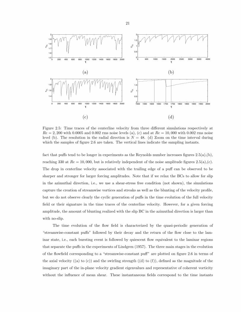
21

!"! "!! #!! $!! %!! &!!! &"!! &#!! &$!! &%!! "!!!

&'(

&'$

&')

&'%

&'*

"

+,-

(a)

!"! "!! #!! $!! %!! &!!! &"!! &#!! &$!! &%!! "!!!

&'(

&'$

&')

&'%

&'*

"

+,-

! "!! #!!! #"!! $!!! $"!! %!!! %"!! &!!!!

!'"

#

#'"

$

()*

+

(b)

!"! "!! #!! $!! %!! &!!! &"!! &#!! &$!! &%!! "!!!

&'(

&'$

&')

&'%

&'*

"

+,-

! "!! #!! $!! %!! &!!! &"!! &#!! &$!! &%!! "!!!

&'#

&'$

&'%

"

+,-

(c)

!"! "!! #!! $!! %!! &!!! &"!! &#!! &$!! &%!! "!!!

&'(

&'$

&')

&'%

&'*

"

+,-

! "!! #!!! #"!! $!!! $"!! %!!! %"!! &!!!!

!'"

#

#'"

$

()*

+

#"!! #""! #,!! #,"! #-!! #-"! #.!! #."! #/!! #/"! $!!!!

!'"

#

#'"

$

()*

(d)

Figure 2.5: Time traces of the centerline velocity from three different simulations respectively atRe = 2, 200 with 0.0005 and 0.002 rms noise levels (a), (c) and at Re = 10, 000 with 0.002 rms noiselevel (b). The resolution in the radial direction is N = 48. (d) Zoom on the time interval duringwhich the samples of figure 2.6 are taken. The vertical lines indicate the sampling instants.

fact that puffs tend to be longer in experiments as the Reynolds number increases figures 2.5(a),(b),

reaching 330 at Re = 10, 000, but is relatively independent of the noise amplitude figures 2.5(a),(c).

The drop in centerline velocity associated with the trailing edge of a puff can be observed to be

sharper and stronger for larger forcing amplitudes. Note that if we relax the BCs to allow for slip

in the azimuthal direction, i.e., we use a shear-stress free condition (not shown), the simulations

capture the creation of streamwise vortices and streaks as well as the blunting of the velocity profile,

but we do not observe clearly the cyclic generation of puffs in the time evolution of the full velocity

field or their signature in the time traces of the centerline velocity. However, for a given forcing

amplitude, the amount of blunting realized with the slip BC in the azimuthal direction is larger than

with no-slip.

The time evolution of the flow field is characterized by the quasi-periodic generation of

“streamwise-constant puffs” followed by their decay and the return of the flow close to the lam-

inar state, i.e., each bursting event is followed by quiescent flow equivalent to the laminar regions

that separate the puffs in the experiments of Lindgren (1957). The three main stages in the evolution

of the flowfield corresponding to a “streamwise-constant puff” are plotted on figure 2.6 in terms of

the axial velocity ((a) to (c)) and the swirling strength ((d) to (f)), defined as the magnitude of the

imaginary part of the in-plane velocity gradient eigenvalues and representative of coherent vorticity

without the influence of mean shear. These instantaneous fields correspond to the time instants

22

!

!

!"#$

!"#%

!"#&

!"#'

"

"#'

"#&

"#%

(a)

!

!

!"#$

!"#%

!"#&

!"#'

"

"#'

"#&

"#%

(b)

!

!

!"#$

!"#%

!"#&

!"#'

"

"#'

"#&

"#%

(c)

0

0.01

0.02

0.03

0.04

0.05

0.06

0.07

0.08

0.09

0.1

(d)

0

0.01

0.02

0.03

0.04

0.05

0.06

0.07

0.08

0.09

0.1

(e)

0

0.01

0.02

0.03

0.04

0.05

0.06

0.07

0.08

0.09

0.1

(f)

Figure 2.6: Contours of the axial velocity, subfigures (a) to (c), and of the swirling strength for thein-plane velocities, subfigures (d) to (f), computed respectively at τ = 1620, τ = 1700, and τ = 1740dimensionless time units.

marked with vertical lines in figure 2.5(d). During the first stage, patches of swirl move toward

the center of the pipe figures 2.6(d),(e) and create streaks by convection of the axial momentum

figure 2.6(a). The radial motion of the coherent swirl corresponds to a lift up of streamwise vortices

away from the wall as observed in the simulations of van Doorne & Westerweel (2009) if we consider

the evolution of the vorticity field projected in a plane moving at the bulk velocity. The second stage

consists of the segregation of the high- and low-speed streaks, the latter being convected toward the

center of the pipe, resulting in the blunting of the velocity profile characteristic of turbulent pipe

flow, figure 2.6(b). Once a low-speed streak reaches the center, the centerline velocity drops sharply,

as can be seen on the time traces on figure 2.5(b). Finally the swirling strength and streaks decay

figures 2.6(c),(f) and the flow returns close to the laminar state before the next cycle starts. As the

streamwise vortices convect toward the center of the pipe, the sign of the net azimuthal velocity is

reversed such that the rotation sign changes from one cycle to the next.

While the output of the 2D/3C model is a temporal variation of a streamwise constant field, a

simplistic comparison with spatial experimental results may be made by assuming an appropriate

convection velocity to be the bulk velocity. With this in mind, the time evolution of the velocity field

is remarkably similar to the flow visualizations by Hof et al. (2004) in transitioning pipe flow when a

puff is observed in a reference frame moving with the bulk velocity. Streak merging in experiments

23

was reported by those authors, who showed that the number of streaks in the cross-section decreases

due to their merging as the cross-stream observation plane is moved from the trailing edge to the

leading edge of a puff. This streak merging, as well as the segregation of the high- and low-speed

streaks observed in the experiments is accurately reproduced by the model, as shown in figure 2.5.

The time evolution of the vorticity field in our simulations is also consistent with the projection of

the three-dimensional vorticity field inside the puff computed by van Doorne & Westerweel (2009)

in a plane moving at the bulk velocity, characterized by a lift up of streamwise vortices away from

the wall as we move from the trailing to the leading edge of the puff (corresponding to increasing

time in our model).

The generation and subsequent decay of the puffs can be described in terms of a simple process

driven by background noise, sketched in the inner loop of figure 2.7. In essence, the presence of

background noise in the pipe cross-section results in the formation of streamwise-constant vortices

which advect axial momentum to create high- and low-speed streaks of axial velocity. The vortices

interact nonlinearly with the streaks to segregate them, i.e., to convect the low-speed streaks toward

the center and the high-speed streaks toward the wall, leading to the blunting of the velocity profile.

We term this a “quasi-self-sustaining process” (QSSP) to reflect the fact that, while there is no

feedback from the axial velocity to the evolution of the streamfunction (denoted by the dashed line

in the inner loop of figure 2.7) which could sustain the cycle described in figure 2.6, the insertion of

small-amplitude stochastic forcing in the cross-stream plane appears to provide an effective replace-

ment for this mechanism. The radial shape of the forcing is directly related to the amount of swirl

present in the simulations and therefore suggests a method to control the flow by shaping the noise

forcing in the spirit of the simple control mechanism developed by Hof et al. (2010) which reduces

the inflection points of the velocity profile and leads to a relaminarization of the flow.

A well-studied, fully self-sustaining process has been described for the (3D/3C) NS equations

by Waleffe (1997), which relies on the nonlinear interaction of the disturbances developing from the

instability of the streaks to force the streamwise vortices. Our results suggest that the blunting of

the velocity profile can be considered to be, in essence, a nonlinear, two-dimensional phenomenon in

which the directional amplification of the 2D/3C model selects the appropriate disturbance shape

from stochastic forcing in order to maintain the QSSP. The model suggests that the sustaining mech-

anisms are therefore insensitive to the type of (nonlinear) interaction invoked to force the streamwise

vortices. Based on the simulations presented here, we argue that it is the presence of appropriate,

small disturbances in the flow (necessarily contained in the white noise of stochastic forcing), and not

their specific interaction that sustains the streamwise vortices and streaks. Hence, the 2D/3C model

shows that using unstructured (stochastic) forcing to generate the streamwise vortices appears to

be sufficient to capture the formation of the streaks and their segregation resulting in a blunting

of the velocity profile and that the overall flow dynamics are relatively insensitive to the particular

24

!"#$%&'(

!"#$%)*+'$(

,-#./$'(

0%/&1#-234((

3-+'$(

54,$/.-3(-6(

)$%3('7$%#(

(((8-#./+"9(/#$%.-3((

%"("7$(*%::(

(;#$%&4-*3(

<-3=>$#-(+3=?:%3$(

,$:-/+"9(

@-3,$/"(

"-*%#4(

/$3"$#(

@:2'"$#+31((

5"("7$((

/$3"$#(#(

A$,$#'$(

#-"%.-3(

'+13(

( !"#$%&()$#1+31(

((((((!"#$%&(

'$1#$1%.-3(

4

Figure 2.7: Diagram detailing the different stages of the QSSP. The dashed lines represent unmodeledeffects.

regeneration process invoked to produce the streamwise vortices. The QSSP is simpler than other

processes described in the literature but does appear to capture the minimum turbulence dynamics

and produce flow fields dominated by streamwise vortices and streaks whose temporal evolution and

topology compares well to experimental visualizations and numerical simulations of puffs, under an

appropriate projection onto a plane convecting at the bulk velocity. In addition, our simulations are

significantly less computationally intensive than studies of the full NS equations (Shimizu & Kida,

2009; van Doorne & Westerweel, 2009) since our domain is 2D and we do not need to track the

position of the puffs in time.

Interestingly, our simulations of the stochastically forced 2D/3C model for pipe flow do not reach

fully developed turbulence, regardless of the amount of forcing and Reynolds number, even though

the same model applied to Couette flow and described in Gayme et al. (2010) reached a steady state

with a velocity profile in good agreement with the profiles from full 3D simulations at the same

Reynolds number, provided that the amount of forcing is appropriately chosen. Mellibovsky et al.

(2009) describe pipe flow transition as a two-stage process, the first stage consists in the formation

of the puffs and the second in their spreading in space. Those authors argue that the two stages are

caused by different instability mechanisms. Our simulations support this point of view since we are

able to capture the first stage using a streamwise-constant model but not the second stage for which

three-dimensional effects are necessary to allow for the puffs to destablize and form slugs which will

expand to cover the whole flow domain.

25

2.5 Summary

A globally-stable, streamwise-constant model of turbulent pipe flow was investigated, and subject to

two types of very simple forcing profiles, namely a deterministic, steady streamfunction and stochas-

tic forcing of the streamfunction equation. By retaining only the nonlinearity coupling the cross-

plane streamfunction and the axial velocity, the model permits the study of the physics underlying

momentum transfer. This model, which is significantly more tractable than the full Navier-Stokes

equations, appears to be capable of capturing key features associated with transition to turbulence,

i.e., the blunting of the velocity profile and the generation of streamwise vortices and streaks.

Using the simplest, time-invariant deterministic forcing, the velocity profile was shown to be

robust with respect to variations in the forcing profile, and to produce realistic velocity fields that

are remarkably similar to the flow visualizations by Hof et al. (2004) near the trailing edge of a puff.

Thanks to the significant reduction in complexity associated with the 2D/3C projection compared to

the full Navier-Stokes equations, several observations can be made by examination of the governing

equations: momentum is extracted from the laminar base flow by (zero-mean) perturbations via

linear non-normal mechanisms and redistributed via nonlinear interactions of the perturbations to

result in a change in mean flow. Hence, the simplistic model allowed for the isolation of the basic

mechanisms leading to the blunting of the velocity profile in pipe flow.

Under stochastic forcing, the model generates “streamwise-constant puffs” at a frequency that

depends on the Reynolds number but not on the forcing amplitude. The model captures the first

stage of pipe flow transition as described in Mellibovsky et al. (2009), i.e., the formation of puffs,

but not the second stage (spreading of the puffs in space) for which some three-dimensional effects

are necessary. The time evolution of the velocity fields produced by the simulations is remarkably

similar to flow visualizations in transitioning pipe flow (Hof et al., 2004) when a puff is observed in

a reference frame moving at the bulk velocity. The segregation of the high- and low-speed streaks

observed in experiments is accurately captured by the model as well as the streak merging and the

lift up of the streamwise vortices away from the wall.

The essential dynamics governing the generation of puffs in pipe flow transition were captured

by the streamwise-constant model and are relatively insensitive to the particular regeneration mech-

anisms invoked to produce the streamwise vortices, permitting the introduction of a “quasi-self-

sustaining process” to describe the generation of puffs and the blunting of the mean velocity profile.

26

Chapter 3

Efficient Representation ofWall-Bounded Turbulence UsingCompressive Sampling

3.1 Introduction

The frequency spectrum of wall-bounded turbulence measured locally in space is known to be broad-

band. For that reason, numerous samples need to be acquired to resolve the frequency content of

the flow and, usually, to satisfy the Nyquist criterion. Most of the samples are, in fact, just needed

to resolve the high-frequency, low-energy modes of the flow, to prevent their aliasing onto lower

frequency modes. The main objective of this chapter is to present and validate a technique, called

compressive sampling, to extract the most energetic frequency modes in wall-bounded turbulence,

using significantly less samples than predicted by the Nyquist criterion. This particularly efficient

technique makes possible the full modal decomposition of turbulent pipe flow in the three spatial

directions and in time, described in the next chapter, by drastically reducing the data storage and

post-processing requirements.

When a sinusoidal signal of frequency f0 is sampled periodically at a rate fs, all the sinusoids of

frequency |f0−Nfs|, where N is an integer, fit the samples, and are called aliases of the fundamental

signal. Bilinskis (2007) suggested that aliasing effects can be eliminated by sampling randomly in

time, because the aliases do not fit the randomized samples. Randomized sampling thereby provides

a way, by sampling at a lower rate than predicted by the Nyquist criterion, to reduce the number

of samples required for perfect reconstruction of the signal. However, if a Fast Fourier Transform

(FFT) is used to extract the frequency content of the samples, fuzzy aliasing (i.e., aliasing that is

more diffuse than in the case of periodic sampling) will occur, because the Fourier basis functions

are not orthogonal on the set of randomized samples. Bilinskis (2007) described several techniques

to remove, or at least attenuate, fuzzy aliasing when a FFT is applied to non-periodic samples. If

27

the signal happens to be sparse in the frequency domain, a compact representation can be efficiently

obtained by applying compressive sampling, instead of using a FFT and correcting for fuzzy aliasing.

In this chapter, it is shown that, if wall-bounded turbulence is decomposed as a sum of propagating

waves (corresponding to Fourier modes in the streamwise and azimuthal directions, and in time), as

explored by McKeon & Sharma (2010), a compact representation can be found, by applying com-

pressive sampling to identify the dominant frequencies of the most energetic spatial Fourier modes.

Compressive sampling has been successfully applied to approximately sparse signals in the tem-

poral domain, e.g., for data compression, and in the spatial domain, mainly for image processing,

to decrease the data storage and postprocessing requirements, see for example Candes et al. (2006),

Lustig et al. (2007), Candes & Wakin (2008). However, the broadband spectrum observed in wall-

bounded turbulence based on spatially localized spectral measurements has previously presented a

barrier to the use of compressive sampling which requires sparsity for efficient performance.

Compressive sampling consists of acquiring randomly in time (or space) a signal that is approxi-

mately sparse in the frequency domain (respectively in wavenumber space), and reconstructing it by

solving a constrained minimization problem. In this thesis, a signal is defined to be sparse if most of

its energy is concentrated in a few basis functions (frequencies), typically 5 or less, implying that a

compact representation of the signal can be obtained by truncating its series representation, keeping

only the most energetic basis functions. This definition of sparsity corresponds to “approximate

sparsity” in the compressed sensing literature. A temporal Fourier basis is chosen to reconstruct

the signal as it is known that, for statistically steady signals, the Fourier basis is optimal in the

sense that it maximizes the energy captured for a given number of basis functions (Liu et al., 2001;

Berkooz et al., 1993).

The Fourier coefficients to reconstruct the signal are obtained by solving a constrained minimiza-

tion problem. The constraints enforce that the reconstructed signal matches the input signal at the

sampling time instants. The minimization problem is based on the `1-norm of the signal, defined

as the sum of the absolute value of its coefficients. Chen et al. (1998) mention that the `1-norm is

particularly adapted to sparse signals as, among all the solutions that meet the constraints, it favors

one with a few large coefficients and a lot of small coefficients. The `1-norm is also convex, implying

that the minimization problem can be solved as a convex optimization problem (Chen et al., 1998),

for which a unique solution exists, provided that the signal is sparse and that the number of samples

is large enough (Candes et al., 2006).

The number of samples, Ns, required for perfect reconstruction of a signal can be estimated using

an empirical relationship by Tropp et al. (2010), henceforth referred to as the sparsity relationship,

Ns ≥ 1.7K log

(Ω

K+ 1

), (3.1)

28

where K is the number of frequencies present in the approximately sparse signal and Ω the bandwidth

or ratio of the highest to lowest frequency of interest. The empirical relationship indicates that the

number of samples increases with the signal bandwidth and the number of sparse frequencies. The

numerical constant 1.7 results from a linear regression on the experimental data obtained by Tropp

et al. (2010), and may be problem specific. The number of samples scales as the logarithm of the

input signal bandwidth, in contrast to the linear scaling associated with periodic sampling, implying

that a significant reduction of the number of samples required to reconstruct the signal can be

obtained for broadband signals containing only a few sparse frequencies.

In practical application of the compressive sampling technique to a randomly sampled signal,

the input frequency range for the constrained minimization problem should be chosen such that

the sparsity relationship is satisfied (equation (3.1)). The minimum and maximum frequencies

(Fourier modes) used to reconstruct the signal can, respectively, be lower than the inverse of the

sampling duration and higher than the mean sampling rate. In contrast, in the case of periodic

sampling, the minimum and maximum frequencies of the Fourier series representing the input signal

are directly related to the sampling parameters: the minimum frequency corresponds to the inverse

of the sampling duration, and the maximum frequency equals the sampling rate for complex-valued

signals and half the sampling rate for real-valued signals.

In this chapter, it is shown using 3D periodically sampled turbulent pipe flow DNS data that,

if the flow fields are Fourier transformed in the homogeneous spatial (wall-parallel) directions, the

frequency content of each Fourier mode is approximately sparse, implying that compressive sampling

can be applied to identify the dominant frequencies. The use of compressive sampling in wall-

bounded turbulence is demonstrated by a series of tests, based on synthetic velocity fields with

known frequency content, aimed at verifying the output from the compressive sampling routine. A

new randomly sampled turbulent pipe flow DNS is analyzed via compressive sampling and shown

to have a compact representation in the form of a superposition of energetic propagating waves.

The frequency content of energetic spatial Fourier modes is shown to be sparse, and can be resolved

using significantly less samples compared to periodic sampling. Results also show that compressive

sampling resolves frequencies up to several times higher than the mean sampling rate.

3.2 Methodology

Two different types of data sets were used to investigate the application of compressive sampling

to wall-bounded turbulence and were based, respectively, on synthetic velocity fields with known

frequency content and turbulent pipe flow DNS data. The cylindrical coordinate system used to

project the flow fields is shown on figure 4.2. The synthetic velocity fields were used to check

that compressive sampling extracts the right frequencies and to determine the optimal sampling

29

!, w

r, v!

x, u

y, v

Figure 3.1: Schematic of pipe geometry and nomenclature (McKeon & Sharma, 2010).

parameters for a new DNS run with velocity fields recorded at random instants in time. Frequency

analysis of the periodically and randomly sampled DNS data was performed to ensure that the

frequency content is approximately sparse and validate the use of compressive sampling in wall-

bounded turbulence, respectively. In the following section, the data sets used in this study are

presented, and the methods to analyze the frequency content of the different flow fields are described.

3.2.1 Synthetic Velocity Fields

Synthetic velocity fields that approximate the DNS propagating waves but have a known frequency

content were generated using the framework of McKeon & Sharma (2010). Generation of these

fields required low computational and storage resources compared to the DNS flow fields, thus they

were used to identify the influence of the sampling parameters on the frequencies extracted via

compressive sampling, for a known set of input frequencies.

McKeon & Sharma (2010) considered a gain analysis of the Navier-Stokes (NS) equations to

obtain a basis for the wall-normal coherence of propagating waves in turbulent pipe flow. In this

approach, the full synthetic velocity field u(x, r, θ, t) was decomposed into a series of propagating

waves defined by their streamwise and azimuthal wavenumbers (k, n) and angular frequency ω = 2πf ,

u(x, r, θ, t) =∑k,n,ω

ak,n,ωck,n,ω(r)ei(kx+nθ−ωt), (3.2)

where the ak,n,ω are complex-valued coefficients denoting the relative magnitude and phase of the

waves. The wavenumbers and frequencies are non-dimensionalized based on the pipe radius and bulk

velocity. Berkooz et al. (1993) showed that the Fourier series decomposition in the homogeneous

(spatial and temporal) directions (equation (3.2)) is optimal in the sense that it maximizes the

turbulent kinetic energy captured for a given number of basis functions and the Fourier modes are

known to be the eigenmodes of the linear NS equations. Under this formulation, the nonlinear terms

in the NS equations for the velocity fluctuations act as an unknown forcing on the linear part of

30

the equations. A divergence-free basis was used in the radial direction to project the NS equations,

resulting in the elimination of the pressure term. The radial distribution of momentum ck,n,ω(r) for

the propagating waves is described by the forced NS equations

iωck,n,ω(r) = Lk,n,ω(r)ck,n,ω(r) + fk,n,ω(r), (3.3)

where fk,n,ω(r) and Lk,n,ω(r) are the projection of the nonlinear terms and of the linear part of the

NS equations onto the Fourier basis, respectively. The propagating wave ck,n,ω(r)ei(kx+nθ−ωt) can

be seen as a response of the mean turbulent flow to the forcing fk,n,ω(r) via the transfer function

(iωI − Lk,n,ω(r))−1, i.e.,

ck,n,ω(r) = (iωI − Lk,n,ω(r))−1fk,n,ω(r). (3.4)

The analysis identifies the forcing and response modes that are most amplified based on a turbulent

kinetic energy norm, at each given wavenumber pair and frequency, via singular value decomposition

(SVD) of the transfer function.

The framework of McKeon & Sharma (2010) was used to generate response modes to represent

wall-bounded turbulence. The synthetic velocity fields were constructed by superposition of response

modes computed with three different (k, n) wavenumber pairs chosen to represent the large scales

(1, 10) modes, the near-wall type modes (4.3, 43) corresponding to a streamwise and azimuthal extent

of 1, 000 and 100 viscous wall-units at Re = 24, 580, and the small dissipative scales (16.75, 60),

respectively. For each wavenumber pair, several convection velocities (frequencies) were chosen

arbitrarily in a range varying from a few viscous units to the centerline velocity. The propagating

waves generated with the three wavenumber pairs and the various frequencies span the broad range

of scales present in wall-bounded turbulence, and their superposition results in realistic velocity fields

due to the coherence in the wall-normal direction. The relative phase of the waves was randomly

chosen and the magnitude was set to one. The propagating waves were computed using the spectral

code of Meseguer & Trefethen (2003) modified by McKeon & Sharma (2010) to allow for the input

of any velocity profile and the decomposition into singular modes. The velocity profile from the

DNS of Wu & Moin (2008) at Re = 24, 580 was used as an input to the model. The synthetic fields

can be sampled at any time instant and require low computational and storage resources compared

to the DNS flow fields, allowing for the test of numerous sampling parameters to use compressive

sampling in wall-bounded turbulence.

Compressive sampling was applied to the streamwise velocity component of the synthetic velocity

fields sampled randomly in time. The velocity fields were decomposed as a Fourier series in the

streamwise and azimuthal directions, and each 2D Fourier mode ck,n(r, ts) was written as a Fourier

31

series in time with unknown coefficients,

ck,n(r, ts) =

Nopti∑j=1

ck,n,2πjdf (r)ei2πjdfts , (3.5)

where Nopti and df are optimization variables (to be determined) corresponding respectively to the

number of frequencies and the frequency increment for the optimization. The coefficients of the

temporal Fourier series ck,n,2πjdf (r) are the solution of an optimization problem that consists of

minimizing the sum of the absolute value of the Fourier coefficients ck,n,2πjdf (r), i.e., minimizing

Nopti∑j=1

|ck,n,2πjdf (r)|, (3.6)

at each wall-normal location separately, under the constraint that the reconstructed signal

Nopti∑j=1

ck,n,2πjdf (r)ei2πjdfts

matches the input signal ck,n(r, ts) at every sampling time instant ts. The dominant Fourier coeffi-

cients ck,n,2πjdf (r) identified via compressive sampling correspond to the streamwise component of

the propagating waves ck,n,ω(r) constituting the synthetic flow field.

Contrarily to periodic sampling, the frequency range for the optimization [df,Nopti × df ] is not

directly related to the sampling parameters, and was chosen to maximize the frequency resolution,

while still satisfying the sparsity relationship (equation (3.1)). For simplicity, the frequencies were

chosen to be equi-spaced within the optimization frequency range (but this is not required in order

to apply compressive sampling). The maximum and minimum frequencies can be respectively higher

than the mean sampling rate and lower than the inverse of the sampling duration. The lower the

number of sparse frequencies present in the input signal the broader the frequency range that can

be resolved with compressive sampling.

The minimization problem was solved with Matlab using the CVX toolbox for convex opti-

mization, and an example of the code used is shown in appendix A. The frequency spectrum was

computed at each wall-normal location, and integrated in the radial direction to identify the ener-

getically dominant frequencies, and to check whether the dominant frequencies matched the input

frequencies. The optimization frequency range and sampling parameters were adjusted to find the

optimal number of samples and sampling duration leading to the recovery of the signal.

32

3.2.2 DNS Velocity Fields

The DNS velocity fields were kindly provided by X. Wu who used the second-order finite difference

code described in Wu & Moin (2008) at Re = 24, 580 (Reτ = 685), and with a domain length

of 30R (kmin = 0.21). The number of grid points in the streamwise, wall-normal, and azimuthal

directions was respectively 2048 × 256 × 1024. The DNS data was subsampled by a factor of 4 in

the streamwise and azimuthal directions to decrease the size of the data files. The flow domain is

large enough for the spatial-averaged velocity profile and streamwise turbulence intensity profile to

be converged, even with the subsampling.

Two sets of velocity fields were available. For the first set, the flow was periodically sampled in

time at a rate of 1 sample every 7.2 dimensionless time units, based on the pipe radius and bulk

velocity. A total of 21 samples was taken over 150 dimensionless time units. The number of samples

and sampling duration for the first data set could not be chosen by the authors and constrained the

number of Fourier modes that could be resolved with the data. The second set was randomly sampled

based on the parameters derived in the present study in order to apply compressive sampling.

The 21 periodically sampled DNS velocity fields were used to check whether the frequency content

of the Fourier modes was indeed sparse. Each velocity field was Fourier transformed in the streamwise

and azimuthal directions by applying a 2D FFT,

u(x, r, θ, t) =∑k,n

ck,n(r, t) ei(kx+nθ), (3.7)

and normalized such that255kmin∑k=0

127∑n=−128

ck,n(r)c∗k,n(r) = u′2(r), (3.8)

where ∗ denotes the complex conjugate and kmin = 0.21 for a domain length of 30R. The 2D

spatial Fourier modes are referred to by their wavenumber pair (k, n). Only the positive k half

plane was kept since the spectrum of a real-valued signal is symmetric. The 2D Fourier spectrum

was integrated in the wall-normal direction and averaged in time to identify the 2D Fourier modes

that contribute most to the streamwise turbulence intensity, effectively a crude POD over a limited

resolvable parameter space.

The range of 2D Fourier modes that were free from aliasing effects was estimated based on their

streamwise wavenumber by comparing the frequency range that can be resolved with the available

DNS data to the empirical bounds on the frequency content of the flow. The dynamically signifi-

cant frequency content in wall-bounded turbulence was estimated as a function of the streamwise

wavenumber by assuming that the highest and lowest convection velocities correspond respectively

to the centerline velocity and 10 times the friction velocity. The upper bound comes from the anal-

ysis of the Orr-Sommerfeld equation by Joseph (1968) showing that, for laminar channel flow, the

33

!"!!

!""

!"!

!"#

!"!#

!"!!

!""

!"!

!

!

"#

$%#&'()&*+,&#

)-./+0/1#&(2)3/'4#

Figure 3.2: Frequency range resolved by the periodically sampled DNS data (delimited by the twohorizontal dashed lines) compared to the empirical upper and lower bounds on the DNS frequencycontent (solid lines) as a function of the streamwise wavenumber k. The shaded area shows thetime-resolved streamwise wavenumber range for the available data.

real part of the eigenvalues, which corresponds to the convection velocity of the disturbances, is

restricted to the range set by the mean flow. The lower bound was estimated based on the results

of Morrison et al. (1971), who used experimental data to decompose the buffer layer as a sum of

propagating waves, and found that the lowest convection velocity is about 10 times the friction

velocity, u = 10uτ , or 0.44U at Re = 24, 580. The value for the lowest convection velocity is broadly

supported in the literature, as summarized by LeHew et al. (2011).

The upper and lower bounds on the frequency content as a function of the streamwise wavenum-

ber are depicted on figure 3.2. The highest frequency that could be resolved with the available DNS

data is given by the inverse of the sampling rate fmax = 17.2 = 0.14 and is reached at k = 0.69

for modes convecting at the centerline velocity. All the modes with k ≥ 0.69 have part of their

frequency content aliased to lower frequencies, such that only the frequency content of the lowest

three streamwise wavenumbers k = 0.21, 0.42, and 0.63, for various azimuthal wavenumbers, could

accurately be extracted from the available DNS data by applying a FFT in time, because the Nyquist

criterion is satisfied for these three modes.

Similarly to the periodically sampled DNS velocity fields, the randomly sampled fields were

decomposed as a Fourier series in the streamwise and azimuthal directions using a 2D FFT, and the

2D Fourier spectrum was integrated in the wall-normal direction and averaged in time, to identify

the most energetic spatial modes. Compressive sampling was used to extract the frequency content

of these most energetic modes at each wall-normal location, following the same methodology as for

the synthetic velocity fields. The frequency spectrum was integrated in the wall-normal direction to

identity the sparse frequencies, defined as the frequencies containing not less than 10% of the energy

34

in the peak frequency.

As an alternative approach, compressive sampling was also applied globally on the `2-norm of

the temporal Fourier coefficients in the wall-normal direction, i.e., to minimize

Nopti∑j=1

∫ 1

0

ck,n,2πjdf (r)c∗k,n,2πjdf (r)rdr, (3.9)

where ∗ denotes the complex conjugate. The 2D Fourier modes were interpolated on a uniform grid

in the radial direction and premultiplied by√r, such that the `2-norm corresponds to the energy

norm in cylindrical coordinates. The latter method only needs to be applied once, instead of at each

wall-normal location separately, and tends to select frequencies that are energetic over a wide range

of wall-normal locations. However, the optimization algorithm converges significantly slower due to

the significant increase in the number of constraints from Ns (the number of samples) to Ns × Nr(the number of samples times the number of grid points in the radial direction). The results obtained

with the two methods were compared to identify the best method to use in wall-bounded turbulence.

3.3 Results

3.3.1 Demonstration of Compressive Sampling Using Synthetic Velocity

Fields

The use of compressive sampling in wall-bounded turbulence was demonstrated by a series of tests,

based on synthetic velocity fields with known frequency content, aimed at verifying the output from

the compressive sampling routine. The frequency content of the synthetic velocity fields was ana-

lyzed to identify the combination of sampling and optimization parameters leading to the correct

estimation of the input frequencies. A representative frequency spectrum is shown on figure 3.3(a).

It was found that taking 30 samples randomly distributed over 100 dimensionless time units was

enough to resolve the frequency content of the synthetic velocity fields. The frequencies inferred via

compressive sampling are reported on table 3.1, and compared to the input frequencies. The relative

error between the input and predicted frequencies is about 1% or less. The frequency increment df

and the number of frequencies for the optimization Nopti result from a balance between satisfying

the sparsity relationship (equation (3.1)) and increasing the frequency resolution. Their value can

be chosen separately for each 2D Fourier mode and is reported on table 3.1.

As a result of the synthetic field tests, the frequency range resolved by compressive sampling

was shown to be significantly broader than the range that could be resolved using periodic sampling,

with the same number of samples and sampling duration. The highest frequency was about 6 times

higher than the mean sampling frequency (fs = 0.3). The limit on the number of sparse frequencies

35

f

y

0 0.02 0.04 0.06 0.08 0.1 0.12 0.14 0.16 0.18 0.2

0.1

0.2

0.3

0.4

0.5

0.6

0.7

0.8

0.9

(a)

f

y

0 0.02 0.04 0.06 0.08 0.1 0.12 0.14 0.16 0.18 0.20

0.1

0.2

0.3

0.4

0.5

0.6

0.7

0.8

0.9

1

(b)

Figure 3.3: Frequency spectrum premultiplied by r as a function of the wall-normal distance y, forthe large-scale mode (k, n) = (1, 10), with the 8 input frequencies reported on table 3.1, sampledduring 100 (a) and 25 (b) dimensionless time units. The distorted contours (b) indicate that thesparsity relationship is not satisfied.

36

Large-scale mode (1,10), Nopti = 600, df = 0.0033Input frequencies 0.091 0.102 0.113 0.122 0.132 0.142 0.163 0.173Output frequencies 0.090 0.103 0.113 0.123 0.133 0.143 0.163 0.173Relative error 1.1% 1.0% 0 0.8% 0.8% 0.7% 0 0

Wall-type mode (4.3,43), Nopti = 900, df = 0.0033Input frequencies 0.309 0.325 0.342 0.488 0.520 0.651 0.813 0.895Output frequencies 0.310 0.327 0.340 0.487 0.520 0.650 0.814 0.892Relative error 0.3% 0.6% 0.6% 0.2% 0 0.2% 0.1% 0.3%

High k mode (16.75,60), Nopti = 900, df = 0.0056Input frequencies 0.618 0.651 0.683 1.627 1.789Output frequencies 0.615 0.650 0.683 1.628 1.788Relative error 0.5% 0.2% 0 0.1% 0.1%

Table 3.1: Parameters and optimization results for the three test cases. The input frequenciescome from the content of the synthetic velocity fields, the output frequencies are those recovered byoptimized compressive sampling.

that could be resolved for a given number of samples and sampling duration was evaluated by adding

more and more sparse frequencies to the synthetic velocity fields. Based on the sparsity relationship

(equation (3.1)) the highest frequency that could be resolved is fmax = 0.64 for the large-scale

and wall-type modes and fmax = 1.66 for the high k mode. The difference comes from the lower

number of sparse frequencies in the high k mode. The estimated maximum frequencies are close to

the ones used in the test cases, supporting that the test cases represent the best that can be done

with the given sampling parameters, and especially that no more than 5 frequencies can be resolved

for the high k mode. Compressive sampling seemed to perform slightly better in the present study

than predicted by the sparsity relationship (equation (3.1)), possibly because the amplitude of the

coefficients was not required to match the input signal up to machine precision as was the case in

the analysis by Tropp et al. (2010), but rather to contain at least 10% of the peak frequency energy.

Figure 3.3 illustrates how the method degrades when the sparsity relationship is no longer sat-

isfied. The frequency spectrum for the large-scale mode is plotted on figure 3.3(a) and exhibits

vertical contours corresponding to frequency peaks that are distinct and relatively far apart. When

the number of sparse frequencies is increased, or the sampling duration (which is related to the re-

solvable bandwidth Ω of the signal in equation (3.1)) decreased, such that the sparsity relationship

is violated, the convex optimization does not recover all the input frequencies, and instead generates

spurious frequencies. As a result, the contours of the frequency spectrum on figure 3.3(b) obtained

by sampling during 25 dimensionless time units (instead of 100) are slanted and contain several in-

correct frequency peaks. The longest timescale of the input signal is 8.85 dimensionless time units,

i.e., about third of the sampling duration.

Based on the frequency analysis of the synthetic velocity fields for various sets of sampling and

37

optimization parameters, it was predicted that 50 samples randomly distributed over 100 dimen-

sionless time units are sufficient to resolve via compressive sampling all the dynamically significant

time scales in turbulent pipe flow at Re = 24, 580. (To be conservative, the number of samples was

increased from the value of 30 used in the test cases to 50.)

3.3.2 Sparsity Check Based on Periodically Sampled DNS Data

Since the compressive sampling technique requires approximate sparsity, in this case in the fre-

quency domain, an explicit check for this condition in wall-bounded turbulence was performed using

periodically-sampled DNS data. The frequency spectrum of the most energetic 2D Fourier modes

was computed as a function of the wall-normal distance by performing a FFT of the 21 samples

available, in time, at each wall-normal location. Only the modes with k ≤ 0.63 which are free from

aliasing effects were considered.

The time average wall-normal profiles of the three most energetic 2D Fourier modes are plot-

ted on figure 3.4. The modes are tall in the wall-normal direction and extend to the centerline.

A representative frequency spectrum corresponding to the mode (0.42, 5) is plotted on figure 3.5

as a function of the wall-normal distance, together with the empirical bounds on the frequency

content, corresponding to convection velocities equal to the centerline velocity and 10 times the

friction velocity, or equivalently 0.44UCL at Re = 24, 580. The frequency spectrum exhibits verti-

cal contours highlighting that the most energetic 2D Fourier modes correspond to a superposition

of propagating waves with constant phase speed, which are coherent in the wall-normal direction.

The frequency content of all the modes studied is always sparse, exhibiting between one and three

dominant frequencies, all the other frequencies contain at least an order of magnitude less energy

than the dominant frequency. The dominant frequencies fall in between the two empirical bounds

on the frequency content. Hence, even though turbulent pipe flow exhibits a continuous frequency

spectrum when measured locally in space, as a result of the sparsity of the 2D Fourier modes in the

frequency domain, compressive sampling can be used in wall-bounded turbulence if the flow fields

are Fourier transformed in the homogeneous directions first.

3.3.3 Frequency Analysis of Randomly Sampled DNS Data via Compres-

sive Sampling

A new run of the turbulent pipe flow DNS was performed by Xiaohua Wu, and the velocity fields

were recorded at the 50 sampling time instants shown on figure 4.1 and randomly distributed over

100 dimensionless time units. The time instants were computed using the optimal sampling param-

eters derived using the synthetic velocity fields. Convex optimization problems were solved using

38

0 0.1 0.2 0.3 0.4 0.5 0.6 0.7 0.8 0.9 10

0.002

0.004

0.006

0.008

0.01

0.012

y

mag

nitu

de

(a)

0 0.1 0.2 0.3 0.4 0.5 0.6 0.7 0.8 0.9 1−6

−5

−4

−3

−2

−1

0

1

2

y

phas

e (u

nits

of p

i)

(b)

Figure 3.4: Wall-normal profile of the magnitude (a) and phase (b) for the first three most energeticmodes (k, n) = (0.21,−2) (dotted), (k, n) = (0.42, 3) (dashed), and (k, n) = (0.21, 2) (solid) of theperiodically sampled DNS flow field.

39

0 0.02 0.04 0.06 0.08 0.1 0.12

0.1

0.2

0.3

0.4

0.5

0.6

0.7

0.8

0.9

!"

#"

Figure 3.5: Representative frequency spectrum corresponding to the 2D Fourier mode (k, n) =(0.42, 5) as a function of the wall-normal distance, with the empirical upper and lower bounds onfrequency, corresponding to convection velocities equal to the centerline velocity and 10 times thefriction velocity, demarcated by the two vertical lines.

0 10 20 30 40 50 60 70 80 90 100ts

Figure 3.6: The 50 DNS sampling time instants randomly distributed over 100 dimensionless timeunits based on the radius and bulk velocity. The last sampling time instant is at τ = 96.57.

CVX, for each energetic 2D Fourier mode extracted from the 50 velocity fields, to obtain their fre-

quency content. The optimization parameters resulting in the highest frequency resolution that still

satisfies the sparsity relationship were determined by analysis of the frequency content of several 2D

Fourier modes. The capabilities of compressive sampling were further tested by investigating how the

method degrades when the sparsity relationship is violated. The optimization can be performed at

each wall-normal location separately, or globally by minimizing the `2-norm of the temporal Fourier

coefficients in the wall-normal direction. The two methods were compared and the best one was

chosen to analyze the frequency content of a broad range of 2D Fourier modes.

It was found by analyzing the frequency content of the DNS 2D Fourier modes that an op-

timization frequency range from −1 to 1 allows for both upstream and downstream propagating

waves, and with a frequency increment of 0.005, results in the highest frequency resolution that can

40

be obtained with the given number of samples. Only the downstream propagating waves carry a

significant fraction of the streamwise turbulence intensity, but the noise is spread over both upstream

and downstream propagating waves, leading to a sparser solution. The fundamental frequency is

fmin = 0.005 or half the inverse of the sampling duration and the number of optimization frequencies

is 400. Using periodic sampling, the flow would have to be sampled for 200 dimensionless time units

in order to obtain a fundamental frequency of 0.005 and 400 samples would be required instead of

50 in the case of compressive sampling.

The solution to the convex optimization problem was shown to be robust with respect to varia-

tions of the fundamental and maximum frequencies, as long as the sparsity relationship is satisfied,

and the maximum frequency is high enough to resolve the noise. When the resolution is increased

by lowering the fundamental frequency, the width of the peak in the power spectral density stays

constant, but the number of frequencies within the peak increases, resulting in a violation of the

sparsity relationship (equation (3.1)). Figure 3.7 shows that, when the resolution is doubled, the

number of sparse frequencies within the peak increases from 2 to 4, and the frequency spectrum as

a function of the wall-normal distance exhibits distorted contours, indicative of a violation of the

sparsity relationship. The minimum number of samples required to resolve correctly the spectrum

on figure 3.7(b) is 32, whereas for the spectrum on figure 3.7(d) 57 samples are needed, but only 50

are available.

When the sparsity relationship is violated, the results degrade differently depending on whether

a global or local minimization is used. In the case of global minimization, the energy is spread over

more frequencies, and the contribution of each dominant frequency to the streamwise turbulence

intensity decreases. The wall-normal profiles of the temporal Fourier modes are still smooth and

span the whole radius. In the case of local minimization, the dominant frequencies can vary slightly

from one wall-normal location to the next, leading to distorted profiles that span only a portion of

the radius, as can be seen on figures 3.8(c),(d) and 3.7(a),(c). The 2D Fourier modes reconstructed

based on the sparse frequencies extracted via compressive sampling do not change when the spar-

sity relationship is no longer satisfied, implying that the same amount of energy is captured by the

sparse frequencies, but distributed differently among them. The sparse frequencies do not change

when the maximum optimization frequency is doubled, keeping the fundamental frequency constant,

illustrating the robustness of the method once the sparsity relationship is satisfied.

Based on the study of several 2D Fourier modes, the sparse frequencies obtained using either

the local or global minimizations were shown to be identical, as were the reconstructed 2D Fourier

modes based on the sparse frequencies. However, the wall-normal profiles of the temporal Fourier

modes were smoother in the case of global minimization (see figure 3.8), justifying the choice of the

global minimization method to analyze the 2D Fourier modes. The frequency content of a broad

range of energetic 2D Fourier modes was analyzed via compressive sampling using the global opti-

41

f

y

0 0.02 0.04 0.06 0.08 0.10

0.2

0.4

0.6

0.8

1

(a)

0 0.02 0.04 0.06 0.08 0.110

−9

10−8

10−7

10−6

10−5

10−4

fPSD

(b)

f

y

0 0.02 0.04 0.06 0.08 0.10

0.2

0.4

0.6

0.8

1

(c)

0 0.02 0.04 0.06 0.08 0.110

−9

10−8

10−7

10−6

10−5

10−4

f

PSD

(d)

Figure 3.7: Power spectral density over the frequency range f ∈ [0, 0.1] as a function of the wall-normal distance (a),(c) and integrated in the wall-normal direction (b),(d) for the 2D Fourier mode(k, n) = (0.21, 2) from the randomly sampled DNS. The top and bottom rows correspond to a localminimization with respectively 400 and 800 optimization frequencies. The dots (b),(d) indicate thesparse frequencies.

42

0 0.2 0.4 0.6 0.8 10

0.005

0.01

0.015

0.02

y

mag

nitu

de

dnsf = 0.030f = 0.035f = 0.0403f

(a)

0 0.2 0.4 0.6 0.8 10

0.005

0.01

0.015

y

mag

nitu

de

dnsf = 0.030f = 0.035f = 0.0403f

(b)

0 0.2 0.4 0.6 0.8 10

0.005

0.01

0.015

0.02

y

mag

nitu

de

dnsf = 0.0325f = 0.0350f = 0.0375f = 0.0400f = 0.04255f

(c)

0 0.2 0.4 0.6 0.8 10

0.005

0.01

0.015

0.02

y

magnitude

dnsf = 0.0325f = 0.0350f = 0.0375f = 0.04004f

(d)

Figure 3.8: Wall-normal profiles of the Fourier modes (k, n, ω) = (0.21, 2, 2πf) from the randomlysampled DNS, for the different dominant frequencies, compared to the time average of the origi-nal and reconstructed signals computed using the local (a) and global (b) minimizations with 400optimization frequencies, and the local (c) and global (d) minimizations with 800 optimization fre-quencies. The maximum frequency for the optimization is 1 in both cases.

mization method and the optimization parameters df = 0.005 and f ∈ [−1, 1].

The most energetic 2D Fourier mode (0.21, 2) was considered as a representative example of

the low streamwise wavenumber modes. Figure 3.7(b) shows that the frequency spectrum in the

range [0, 0.1] contains two sparse frequencies f = 0.035 and 0.040, with an energy content of not

less than 10% of the peak value. The power spectral density over the full frequency range used for

the optimization is shown on figure 3.9. Most of the energy is concentrated in the range [0, 0.1] and

the higher frequencies, as well as the negative frequencies corresponding to upstream propagating

modes, only capture the noise. The noise floor is about 5 orders of magnitude lower than the peak.

The presence of negative optimization frequencies is required for the optimization to converge, unless

the highest optimization frequency is increased. It is found that sparser solutions are obtained using

both positive and negative optimization frequencies, instead of increasing the upper bound on the

optimization frequencies. The optimization will not converge if the frequency range is restricted to

[0, 0.1] because the high frequency noise above the noise floor cannot be resolved. The temporal

43

−1 −0.8 −0.6 −0.4 −0.2 0 0.2 0.4 0.6 0.8 110−25

10−20

10−15

10−10

10−5

100

f

Four

ier c

oeffi

cien

t am

plitu

de2

Figure 3.9: Power spectral density for the 2D Fourier mode (k, n) = (0.21, 2) from the randomlysampled DNS obtained via optimal compressive sampling.

Fourier modes corresponding to the three dominant frequencies f = 0.030, 0.035, and 0.040 of the

2D Fourier mode (0.21,2) are plotted on figure 3.8(b), and together contain 91% of the streamwise

turbulence intensity compared to 52% for the peak frequency alone. The frequency f = 0.030 is not

considered to be a sparse frequency, based on the criterion that sparse frequencies need to contain

at least 10% of the peak energy, but is retained as a dominant frequency such that the superposition

of the three dominant frequencies captures over 90% of the energy in the 2D Fourier mode (0.21, 2).

The 2D Fourier modes can be reassembled by summation over the temporal Fourier modes cor-

responding to the sparse frequencies. The presence of dominant frequencies adjacent to the peak

frequency provides for the amplitude modulation of the 2D Fourier modes. Figure 4.8(a),(b) shows

that the 2D Fourier mode (0.21, 2) can be reconstructed with only three temporal Fourier modes

(sparse frequencies) and the relative phase of the modes captures the increase in magnitude of the

2D Fourier mode observed particularly from the first to the second period.

Another two 2D Fourier modes (1.05, 2) and (3.14, 4) were selected for illustration purposes and

represent the range of streamwise wavenumbers that can be analyzed with the 50 velocity fields avail-

able. The contours of the real part of the two 2D Fourier modes in a wall-normal-temporal plane are

plotted on figure 3.11(a),(c) and the wall-normal profile of their dominant temporal Fourier modes

is shown on figure 3.11(b),(d). A comparison between figures 4.8 and 3.11 shows that the extent of

the uniform momentum zones in the wall-normal direction decreases as the streamwise wavenumber

increases, and the reconstructed modes contain less and less energy near the wall, due to the ap-

pearance of two different types of uniform momentum zones in the wall-normal direction, identified

visually on figure 3.11(c) above and below y = 0.1R. Close to the wall, the uniform momentum

44

t

y

0 20 40 60 800

0.2

0.4

0.6

0.8

1

−0.015

−0.01

−0.005

0

0.005

0.01

0.015

(a)

t

y

0 20 40 60 800

0.2

0.4

0.6

0.8

1

−0.015

−0.01

−0.005

0

0.005

0.01

0.015

(b)

Figure 3.10: Contours of the real part of the 2D Fourier mode (k, n) = (0.21, 2) from the randomlysampled DNS, as a function of the wall-normal distance and time, with all the frequencies included(a) and with only three dominant frequencies recovered from compressive sampling included (b).

zones are short in the wall-normal direction whereas further from the wall, the uniform momentum

zones have a radial wavelength of about a quarter radius inferred from the sharp peak in the radial

power spectrum in figure 3.12(a). The spectrum is obtained by applying a FFT to the data without

windowing since the profiles vanish at the boundaries (the wall and the centerline), and can therefore

be assumed periodic with a fundamental wavelength equal to R. Using a sharp Fourier filter with a

cutoff at the fourteenth mode, the near-wall type uniform momentum zones were separated from the

core uniform momentum zones in the wall-normal direction. Figure 3.12(b),(c) shows the contours

of the real part of the 2D Fourier mode (3.14, 4) Fourier filtered in the radial direction. The sharp

Fourier filter successfully separated between the two different types of uniform momentum zones, as

can be seen by comparing figure 3.12(b),(c) to figure 3.12(a). A minimization problem was solved

separately for the two types of uniform momentum zones to extract their respective frequency con-

tent. The frequency content of the near-wall uniform momentum zones was shown to be broadband

and could not be captured using compressive sampling with the chosen sampling parameters, justi-

fying the decrease in the energy captured near the wall as k increases observed on figure 3.11(b),(d).

Compressive sampling was applied to a broad range of 2D Fourier modes, and successfully

captured the frequency content in the core of the pipe for most of the energetic 2D Fourier modes

ranging in size from the largest modes (k = 0.21) all the way down to the near-wall type modes

of size λ+ = 1, 000 (k = 4.3), supporting that the frequency content is indeed sparse. The fre-

quency content of all the dominant modes studied is represented on figure 3.13(a) as a function

of the streamwise wavenumber. Within a resolution error of df = ±0.0025, all the frequencies fall

in between the lower and upper empirical bounds corresponding to convection velocities equal to

respectively 10 times the friction velocity and the centerline velocity.

45

t

y

0 20 40 60 80

0.1

0.2

0.3

0.4

0.5

0.6

0.7

0.8

0.9

−0.01

−0.005

0

0.005

0.01

(a)

0 0.2 0.4 0.6 0.8 10

1

2

3

4

5

6

7

8x 10−3

ym

agni

tude

dnsf = 0.155f = 0.175f = 0.1803f

(b)

t

y

0 20 40 60 80

0.1

0.2

0.3

0.4

0.5

0.6

0.7

0.8

0.9

−5

0

5x 10−3

(c)

0 0.2 0.4 0.6 0.8 10

0.5

1

1.5

2

2.5

3x 10−3

y

mag

nitu

de

dnsf = 0.450f = 0.495f = 0.500f = 0.5404f

(d)

Figure 3.11: Contours of the real part of the 2D Fourier modes (k, n) = (1.05, 2) (a) and (k, n) =(3.14, 4) (c) from the randomly sampled DNS as a function of the wall-normal distance and time.Wall-normal profiles of the Fourier modes (k, n, ω) = (1.05, 2, 2πf) (b) and (k, n, ω) = (3.14, 4, 2πf)(d) for the different sparse frequencies compared to the time average of the original and reconstructedsignals.

46

10 20 30 40 500

0.01

0.02

0.03

0.04

0.05

0.06

q

magnitude

(a)

t

y

0 10 20 30 40 50 60 70 80 900

0.2

0.4

0.6

0.8

1

(b)

t

y

0 10 20 30 40 50 60 70 80 900

0.2

0.4

0.6

0.8

1

(c)

Figure 3.12: (a) Time-averaged power spectral density in the wall-normal direction for the 2D Fouriermode (k, n) = (3.14, 4) from the randomly sampled DNS. (b) Contours of the real part of the 2DFourier mode (k, n) = (3.14, 4) low-pass filtered and (c) high-pass filtered showing the two differenttypes of uniform momentum zones present in the wall-normal direction.

47

!"!!

!""

!"!

!"#

!"!#

!"!!

!""

!"!

$

%

(a)

!"!!

!""

!"!

!"#

!"!#

!"!!

!""

!"!

$

%

(b)

Figure 3.13: Frequency content of the 2D Fourier modes as a function of the streamwise wavenumberfor various azimuthal wavenumbers (a). The two solid lines indicate the upper and lower empiricalbounds on the frequency content and the dashed line shows the streamwise wavenumber correspond-ing to the near-wall type modes. The shaded areas highlight the dynamically significant bandwidthand streamwise wavenumber range at Re = 24, 580 (a) and extrapolated to Re = 300, 000 (b).

3.3.4 Comparison with Periodic Sampling

Compressive sampling was compared with periodic sampling to emphasize the superiority of the

former method in resolving the frequency content of the most energetic 2D Fourier modes, when

only a limited amount of data is available. The data set corresponding to the periodically sampled

DNS run contained 21 velocity fields distributed over 150 dimensionless time units, whereas for the

randomly sampled DNS run, 50 fields were available and distributed over 100 dimensionless time

units. The first 14 velocity fields of the periodically sampled DNS run were used to estimate the

frequency content of the most energetic 2D Fourier modes via a FFT of the data in time. The

minimum and maximum frequencies for the FFT are given by fmin = 0.01 and fmax = 0.13. Only

the 2D Fourier modes corresponding to the lowest three streamwise wavenumbers could be resolved,

the other modes have their frequencies aliased to the range [0.01, 0.13].

Compressive sampling was applied on 14 velocity fields randomly chosen among the 50 fields

available to match the sampling duration and number of samples of the periodic data. The fre-

quency content of the most energetic 2D Fourier modes could be resolved for k ≤ 1.47 instead of

k ≤ 4.3 when the 50 samples were used. The dominant frequencies and their energy content are

reported on table 3.2 for 5 representative 2D Fourier modes. The frequencies obtained match rel-

atively well the results from the FFT, especially for the first two modes studied, even though two

different runs of the DNS were used to generate the samples. The sparse frequencies obtained by

compressive sampling with either 14 or 50 samples are identical, but the wall-normal profiles of the

temporal Fourier modes vary slightly, see figure 3.14. The energy content of the sparse frequencies is

higher when 14 samples are used instead of 50, and is also higher than for the frequencies obtained

48

(k,n) f (CS) % u′2 (CS) f (FFT) % u′2 (FFT)(0.21,2) 0.035 82 0.03 51

0.040 14 0.04 20(0.42,-3) 0.065 95 0.06 21

0.07 58(0.63,-2) 0.09 23 0.08 50

0.105 29 0.110 270.110 23 – –

(1.05,2) 0.180 59 – –(1.47,2) 0.255 15 – –

0.260 25 – –0.265 8 – –

Table 3.2: Frequency analysis of 5 representative modes using only 14 snapshots acquired over 100dimensionless time units from two different runs of the turbulent pipe flow DNS. The dominantfrequencies obtained via compressive sampling analysis of the randomly sampled DNS and theirstreamwise energy content are reported in the second and third columns, respectively. The fourthand fifth columns correspond to the frequencies and respective energy content obtained by FFT ofthe periodically sampled DNS.

via FFT with respectively 96% vs. 71% of the energy in the dominant frequencies for the first mode,

and 95% vs. 79% for the second. In other words, the compressive sampling solution requires less

basis functions (frequencies) to capture a set percentage of streamwise turbulence intensity than the

solution obtained with periodic sampling.

The advantage of compressive sampling over periodic sampling in the case of approximately

sparse data will become even more evident at higher Reynolds number, because the dynamically

significant frequency range increases with Reynolds number. Figure 3.13(b) shows the broadening of

the frequency range resulting from an increase in Reynolds number by one order of magnitude com-

pared to figure 3.13(a), implying that ten times more samples are needed to resolve the frequency

content via periodic sampling. The number of samples required for compressive sampling scales

as the logarithm of the bandwidth, leading to an exponential gain in terms of number of samples

compared to periodic sampling.

Compressive sampling also provides a way to increase the frequency resolution as many more

frequencies can be chosen to perform the optimization than the number of samples available. Fig-

ure 3.15 illustrates how the frequency resolution can be increased by using compressive sampling as

opposed to periodic sampling. The sampled signal is composed of three Fourier modes ei2πft with

frequencies f = 0.035, 0.052, 0.087 and unit magnitude, sampled 50 times over 100 time units. In

the case of periodic sampling, the minimum and maximum frequencies are given by fmin = 0.01 and

fmax = 0.49, and the PSD is shown on figure 3.15(a). The maximum frequency nearly equals the

sampling frequency (not half the sampling frequency because the input signal is complex-valued).

In the case of compressive sampling, two different resolutions were tested. The first one matches

the periodic sampling case, df = fmin = 0.01 and the second one is ten times higher df = 0.001.

49

0 0.1 0.2 0.3 0.4 0.5 0.6 0.7 0.8 0.9 10

0.002

0.004

0.006

0.008

0.01

0.012

0.014

0.016

0.018

y

mag

nitu

de

DNSf=0.035 Ns=14f=0.035 Ns=50f=0.040 Ns=14f=0.040 Ns=50

Figure 3.14: Comparison between the time-averaged wall-normal profile of the 2D Fourier mode(k, n) = (0.21, 2) from the randomly sampled DNS and its two sparse frequencies obtained usingcompressive sampling with 14 and 50 snapshots.

The PSDs are plotted on figure 3.15(b),(c) and show that for the higher-resolution case the three

input frequencies were recovered exactly, because the set of Fourier modes used for the optimization

includes the three input frequencies. For the lower resolution case, the PSD obtained via compressive

sampling exhibits a lower level of noise, or equivalently, a sparser solution than the PSD obtained

via FFT of periodic samples.

3.4 Summary

A novel application of compressive sampling to extract the frequency content of energetic modes in

wall-bounded turbulence was presented. It was shown that compressive sampling can be applied if

the flow field is expanded as a Fourier series in the homogeneous wall-parallel directions, as proposed

by McKeon & Sharma (2010).

The use of compressive sampling in wall-bounded turbulence was validated by performing tests

based on synthetic velocity fields with known frequency content that approximate the DNS flow

fields. Compressive sampling successfully extracted the correct frequencies from the synthetic flow

fields, and did so with significantly fewer samples than predicted by the Nyquist criterion. Equiva-

lently, compressive sampling was shown to be able to resolve frequencies up to six times higher than

the mean sampling rate.

Frequency analysis of periodically sampled turbulent pipe flow DNS data revealed that the fre-

50

0 0.1 0.2 0.3 0.4 0.5

10−20

10−10

100

f

PSD

(a)

0 0.1 0.2 0.3 0.4 0.5

10−20

10−10

100

f

PSD

(b)

0 0.1 0.2 0.3 0.4 0.510−25

10−20

10−15

10−10

10−5

100

f

PSD

(c)

Figure 3.15: Power spectral density of a superposition of three Fourier modes with unit magnitudeand frequencies f = 0.035, 0.052, 0.087 sampled 50 times during 100 time units computed using (a)periodic sampling with FFT, and (b) compressive sampling with a frequency increment of df = 0.01and (c) df = 0.001.

51

quency content of each 2D Fourier mode is indeed approximately sparse. The 2D Fourier modes

correspond to a superposition of propagating waves that are coherent in the wall-normal direction,

and convect downstream at a speed between 10 times the friction velocity and the centerline veloc-

ity. It was predicted that 50 samples, randomly distributed over 100 dimensionless time units, are

sufficient to resolve via compressive sampling all the dynamically significant time scales in turbulent

pipe flow at Re = 24, 580.

Compressive sampling was applied to a broad range of energetic 2D Fourier modes of streamwise

extent varying from the longest modes (k = 0.21) to the near-wall type modes (k = 4.3, λ+ = 1, 000)

at Re=24,580. The frequency content was shown to be approximately sparse, and falls in between

the two empirical bounds on the convection velocity, corresponding to modes convecting at 10 times

the friction velocity and the centerline velocity. The frequencies obtained via compressive sampling

are robust with respect to variations of the optimization parameters, as long as the sparsity rela-

tionship is satisfied.

When only a limited amount of data is available, compressive sampling can resolve more 2D

Fourier modes than periodic sampling, and results in higher frequency resolution. The advantage of

compressive sampling over periodic sampling will become even more evident as higher Reynolds num-

bers are reached by numerical simulations resulting in broader dynamically significant bandwidths,

since the number of samples required to resolve a given bandwidth with compressive sampling scales

as the logarithm of the bandwidth instead of linearly.

Compressive sampling is used in the next chapter to significantly reduce the data requirements

for a full modal decomposition of turbulent pipe flow, in the three spatial directions and in time,

and results in sparse representations of the flow in the frequency domain.

52

Chapter 4

Sparse Representation of TurbulentPipe Flow by Propagating Wavesand a Model-Based Radial Basis

4.1 Introduction

A variety of measurements in wall-bounded turbulence has revealed the presence of coherent and

persistent structures extending over large regions of the flow domain. While many definitions of

coherent structures exist in the literature, Berkooz et al. (1993) offer a description of organized

spatial features which repeatedly appear and evolve in time in a characteristic way; this is the

definition we will adopt in this work.

Recently, Smits et al. (2011) categorized coherent structures in order of increasing streamwise

lengthscale as follows: the well-known (and well-studied) near-wall streaks identified by Kline et al.

(1967), the horseshoe or hairpin vortices described by Theodorsen (1952), large scale motions (LSMs)

of the order of the outer flow lengthscale that are thought to constitute the packets of hairpins

detailed by Adrian (2007), and the very large scale motions (VLSMs) of order ten times the outer

lengthscale, e.g., Kim & Adrian (1999). Experimental capture of this full range of coherent structures

can be extremely challenging due to their large extents in the wall-parallel directions, evolution and

varying degree of localization in the wall-normal direction. This translates to the requirement for

high spatial resolution, large field-of-view, time-resolved simultaneous volumetric measurements of

the velocity field, a challenge even for the state-of-the-art volumetric experimental techniques such

as tomographic or holographic particle image velocimetry (PIV). Planar measurements that meet

the spatial resolution requirements have been reported in the literature for several years, e.g., the

streamwise wall-normal plane measurements of Meinhart & Adrian (1995), while relatively recent

advances in the temporal capability of commercial systems have enabled time-resolved measurements

in the wall-parallel plane, albeit at relatively low turbulent Reynolds numbers (Dennis & Nickels,

53

2008; LeHew et al., 2011).

While significant progress has been made in identifying each class of coherent structures over

the past couple of decades, efforts to assemble low-order models that capture both statistical and

structural information have been generally less successful. In particular, the correct bases by which

to characterize them remains a question of current investigation.

One such approach is the decomposition of wall-bounded turbulence into modes ranked by en-

ergetic contribution, obtained by Proper Orthogonal Decomposition (POD). POD is defined based

on an inner product (ga,gb), a norm ||g||, and an averaging operation 〈.〉 (Berkooz et al., 1993). In

turbulence, the inner product is usually chosen to correspond to the turbulent kinetic energy

(ga,gb) =

∫Ωfl

3∑i=1

ga,i(X)gb,i(X)dX, (4.1)

where ga and gb are zero-mean 3-component velocity fields, Ωfl is the flow domain, and the norm

is defined as ||g|| = (g,g)12 . Liu et al. (2001) showed that the POD basis is optimal in the sense

that the POD expansion converges faster than any other modal expansion based on the energy norm

(equation (4.1)). The 3 components of velocity POD modes Φ(X) correspond to the eigenmodes of

the ensemble averaged velocity cross-correlation tensor

∫Ωfl

〈u(X)u(X ′)〉Φ(X ′)dX ′ = λΦ(X). (4.2)

The POD modes for the streamwise velocity fluctuations are denoted φ(X) and are eigenmodes of

∫Ωfl

〈u(X)u(X ′)〉φ(X ′)dX ′ = λφ(X). (4.3)

In the statistically homogeneous directions, Berkooz et al. (1993) showed that the POD modes

correspond to Fourier modes. Thus, for a fully-developed case such as turbulent pipe flow, for which

the only inhomogeneous direction is the wall-normal one, the full POD modes take the form

Φ(x, r, θ, t) =∑k,n,ω

ck,n,ω(r)ei(kx+nθ−ωt), (4.4)

where (x, r, θ) are the streamwise, radial and azimuthal directions normalized by the pipe radius,

respectively, and (k, n, ω) are the streamwise and spanwise wavenumbers and the temporal (angular)

frequency. The wall-normal distance y is also normalized by the pipe radius (or the channel half-

height when referring to channel flow studies). The wall-normal coherence of the structures is

captured through the functions ck,n,ω(r), the basis for which is to be determined. This representation

enforces homogeneity in the streamwise and azimuthal/spanwise directions and statistical steadiness.

54

The POD kernel is then parameterized by (k, n, ω), and depends only on the wall-normal distance;

however determining this full kernel from observations involves averaging over many time-resolved

flow realizations, which requires acquiring and processing a very significant amount of data.

To reduce the data requirements, averaging in one or more homogeneous directions or in time is

commonly used instead of Fourier decomposition to approximate the POD kernel. Duggleby et al.

(2009) compared the Fourier method (based on time average) to the method of snapshots (based

on spatial average) to compute the POD modes, and showed that the former method converges

faster, but requires more modes to capture a set percentage of the energy in a given finite-time

realization. Those authors emphasized that the two methods should yield the same basis functions

as the sampling duration tends to infinity. Here, we review some recent studies to highlight the

implementation and effects of decreasing amounts of averaging.

Baltzer & Adrian (2011) performed a POD of the streamwise velocity fluctuations of a Direct

Numerical Simulation (DNS) of turbulent channel flow at Reτ=180, 395, and 934, based on averaging

in the two homogeneous directions (x, z) and in time. The POD modes then simplify to functions

of the wall-normal distance, y, alone,

φ(x, y, z, t) = c(y), (4.5)

and are solutions of the eigenvalue problem

∫ 1

−1

〈u(y)u(y′)〉c(y′)dy′ = λc(y), (4.6)

where 〈.〉 denotes an average over the streamwise and spanwise directions and in time. The resultant

POD modes were characterized as either large scale or small scale. The large-scale modes captured

most of the energy and were specific to the flow configuration, whereas the small-scale modes con-

tributed most to the energy dissipation and were hypothesized to be asymptotically self-similar and

universal.

Hellstroem et al. (2011) used 2D+time Particle Image Velocimetry (PIV) in the cross-stream

plane in a turbulent pipe flow at Re=12,500 (Reτ ≈ 375, computed based on the friction factor

measured at Re=13,650 by Swanson et al. (2002)) to perform a POD of the streamwise velocity

fluctuations in physical space, without spatial averaging or Fourier decomposition, to investigate the

structure of the VLSMs. There the POD modes took the form

φ(x, r, θ, t) = φ(r, θ, t), (4.7)

such that ∫ T

0

∫ 2π

0

∫ 1

0

〈u(r, θ, t)u(r′, θ′, t′)〉φ(r′, θ′, t′)r′dr′dθ′dt′ = λφ(r, θ, t), (4.8)

55

where 〈.〉 here denotes an average over several flow realizations. The time evolution of the POD

modes was converted into streamwise evolution using Taylor’s hypothesis and the local mean velocity,

leading to a set of three-dimensional POD modes. The results showed that only a small number of

modes was required to reconstruct characteristics of the VLSMs.

Duggleby et al. (2007) performed a POD analysis of turbulent pipe flow DNS data at Re = 4300

(Reτ = 150) using a Fourier decomposition in the streamwise and azimuthal directions and a time

average. The POD modes,

Φ(x, r, θ, t) =∑k,n

ck,n(r)ei(kx+nθ), (4.9)

were obtained by solving

∫ 1

0

〈uk,n(r)u∗k,n(r′)〉ck,n(r′)r′dr′ = λk,nck,n(r), (4.10)

where 〈.〉 here denotes a time average, and ∗ the complex conjugate. The full flow field was repre-

sented as a sum of POD modes

u(x, r, θ, t) =∑k,n,q

ak,n,q(t)ck,n,q(r)ei(kx+nθ), (4.11)

where q is the POD mode order, or quantum number (corresponding in this case to the number of

zero crossings of the mode amplitude plus one) and the ak,n,q(t) are amplitude coefficients obtained

by projection of the POD modes onto the flow field. The POD modes were classified either as prop-

agating or nonpropagating. The propagating modes had a constant phase speed and time-varying

magnitude; such modes were shown to capture 89% of the total turbulent kinetic energy. The physi-

cal interpretation is of propagating waves that evolve (grow and decay) in time, highlighting that the

statistical steadiness of the flow is not enforced and a manifestation of lack of temporal convergence.

When the Fourier decomposition is applied in all homogeneous directions and in time, the re-

sulting modal expansion of the flow field associated with the modes given by eqaution (4.4),

u(x, r, θ, t) =∑k,n,ω

ck,n,ω(r)ei(kx+nθ−ωt), (4.12)

can be interpreted as a sum of propagating waves with complex-valued coefficients ck,n,ω(r), param-

eterized by a wavenumber pair and frequency, and with variation in the wall-normal distance. Such a

parametrization is consistent with the usual spectral representation of data obtained in experiments

and simulation. However, further physical insight can also be obtained; Morrison et al. (1971) used

experimental data to decompose the buffer layer as a sum of propagating waves, and concluded

that the propagating waves are of dynamical importance due to their coherence in the wall-normal

56

direction.

In practice, the numerous time-resolved 3D realizations of the flow required to assemble the ideal

POD kernel and to ensure the data independence of the basis functions have precluded the use of

a data-based POD kernel for the modal decomposition of the propagating waves. One method of

reducing the data requirements is to introduce a model basis for the radial direction and form what

we will term a model-based kernel. McKeon & Sharma (2010) described such a basis in their systems

analysis of turbulent pipe flow. Since this basis will be used in the work described below, we will

give a brief introduction to the approach here.

The analysis presented by McKeon & Sharma (2010) utilized a Fourier decomposition of the

Navier-Stokes (NS) equations in the homogeneous directions (for the reasons given above, these are

the optimal bases), such that the velocity field can be written as the sum of propagating waves

u(x, r, θ, t) =∑k,n,ω

ak,n,ωck,n,ω(r)ei(kx+nθ−ωt), (4.13)

where the ak,n,ω are complex-valued coefficients representing the relative magnitude and phase of

the waves. The (normalized) radial basis functions, called velocity response modes, ck,n,ω(r), are

to be determined but are constrained to be divergence free in order to eliminate the influence of

pressure. For each (k, n, ω), then, the NS equations can be written in the form

iωck,n,ω(r) = Lk,n,ω(r)ck,n,ω(r) + fk,n,ω(r), (4.14)

where fk,n,ω(r) is the projection of the nonlinear terms onto the Fourier basis and

Lk,n,ω(r) =

ARe−1 + ikU BRe−1 0

−BRe−1 ARe−1 + ikU 0

−∂rU 0 (A− r−2)Re−1 + ikU

, (4.15)

where A = −∂rr − r−1∂r + n2r−2 + k2 + r−2, B = 2inr−2 and the mean flow velocity profile

U = (0, 0, U)T constitutes an input to the analysis. The first to third lines of the resolvent correspond

to the radial, azimuthal, and streamwise velocity components, respectively.

Under this formulation, the velocity can be seen as a response of the flow system to the forcing

fk,n,ω(r) via the transfer function Hk,n,ω = (iωI − Lk,n,ω(r))−1, commonly called the resolvent

(Trefethen & Embree, 2005), i.e.,

ck,n,ω(r) = Hk,n,ωfk,n,ω(r) = (iωI − Lk,n,ω(r))−1fk,n,ω(r). (4.16)

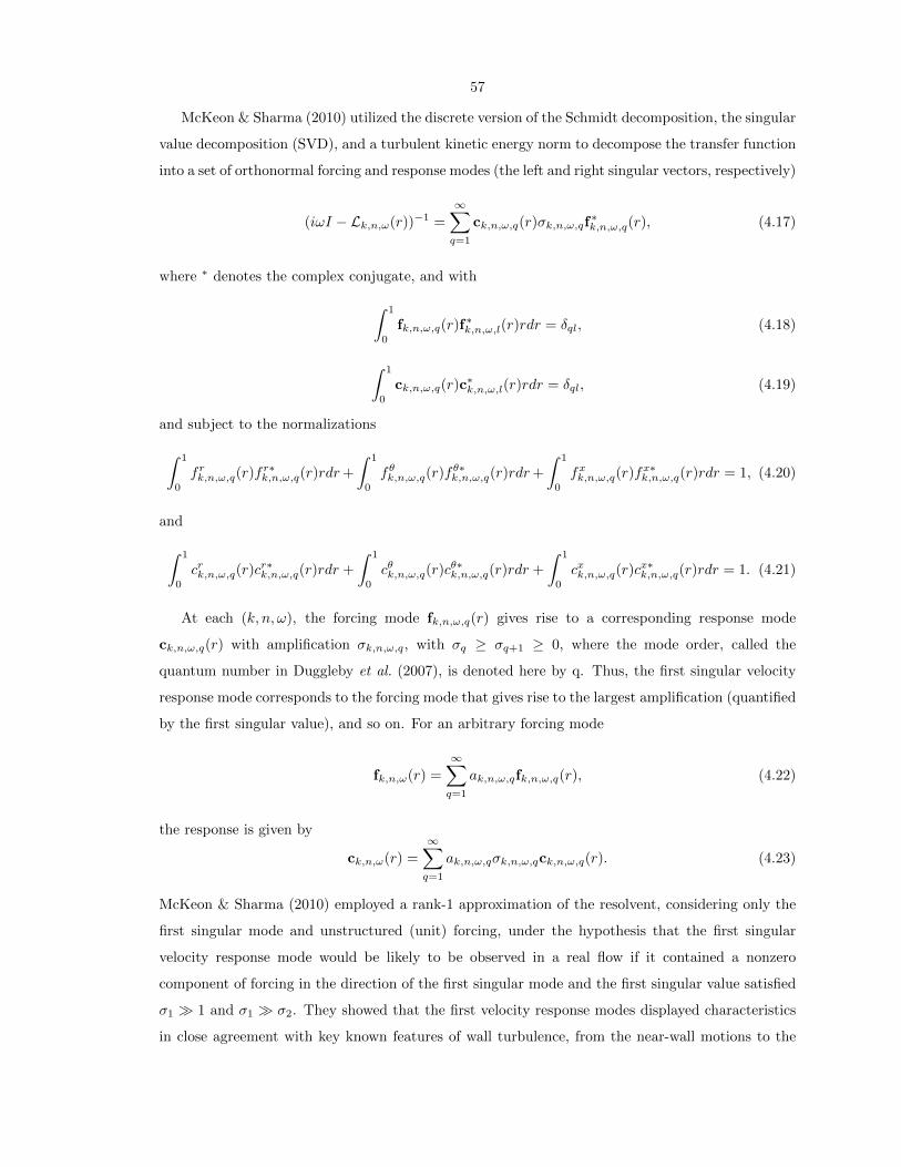
57

McKeon & Sharma (2010) utilized the discrete version of the Schmidt decomposition, the singular

value decomposition (SVD), and a turbulent kinetic energy norm to decompose the transfer function

into a set of orthonormal forcing and response modes (the left and right singular vectors, respectively)

(iωI − Lk,n,ω(r))−1 =

∞∑q=1

ck,n,ω,q(r)σk,n,ω,qf∗k,n,ω,q(r), (4.17)

where ∗ denotes the complex conjugate, and with

∫ 1

0

fk,n,ω,q(r)f∗k,n,ω,l(r)rdr = δql, (4.18)

∫ 1

0

ck,n,ω,q(r)c∗k,n,ω,l(r)rdr = δql, (4.19)

and subject to the normalizations

∫ 1

0

frk,n,ω,q(r)fr∗k,n,ω,q(r)rdr+

∫ 1

0

fθk,n,ω,q(r)fθ∗k,n,ω,q(r)rdr+

∫ 1

0

fxk,n,ω,q(r)fx∗k,n,ω,q(r)rdr = 1, (4.20)

and

∫ 1

0

crk,n,ω,q(r)cr∗k,n,ω,q(r)rdr +

∫ 1

0

cθk,n,ω,q(r)cθ∗k,n,ω,q(r)rdr +

∫ 1

0

cxk,n,ω,q(r)cx∗k,n,ω,q(r)rdr = 1. (4.21)

At each (k, n, ω), the forcing mode fk,n,ω,q(r) gives rise to a corresponding response mode

ck,n,ω,q(r) with amplification σk,n,ω,q, with σq ≥ σq+1 ≥ 0, where the mode order, called the

quantum number in Duggleby et al. (2007), is denoted here by q. Thus, the first singular velocity

response mode corresponds to the forcing mode that gives rise to the largest amplification (quantified

by the first singular value), and so on. For an arbitrary forcing mode

fk,n,ω(r) =

∞∑q=1

ak,n,ω,qfk,n,ω,q(r), (4.22)

the response is given by

ck,n,ω(r) =

∞∑q=1

ak,n,ω,qσk,n,ω,qck,n,ω,q(r). (4.23)

McKeon & Sharma (2010) employed a rank-1 approximation of the resolvent, considering only the

first singular mode and unstructured (unit) forcing, under the hypothesis that the first singular

velocity response mode would be likely to be observed in a real flow if it contained a nonzero

component of forcing in the direction of the first singular mode and the first singular value satisfied

σ1 1 and σ1 σ2. They showed that the first velocity response modes displayed characteristics

in close agreement with key known features of wall turbulence, from the near-wall motions to the

58

VLSMs, and appeared to obey the scalings obtained from classical (viscous) critical layer analysis,

despite the cylindrical coordinate system in the pipe.

Experimental mean flow velocity profiles, U = (0, 0, U)T , were used to form the resolvent in this

study, but the analysis can be made self-consistent in the sense that the mean profile is supported

by the Reynolds stresses associated with all (k, n, c, q) modes if the ak,n,ω,q are chosen appropriately

(equivalent to structuring the forcing correctly for maintenance of the turbulence). While the work

of McKeon & Sharma (2010) was analytical, a data-driven approach can be used to project out

the ak,n,ω,q coefficients from direct numerical simulation; this is the primary function of the present

chapter.

The previous chapter explored the use of compressive sampling in wall-bounded turbulence to

perform such a projection (in essence equivalent to obtaining the full POD kernel described earlier),

and the concomitant reductions in data storage required to project out the velocity response modes

from direct numerical simulations of turbulent pipe flow. We apply this technique here in order to

obtain sparse representations of the flow to investigate the structure of turbulence and its sustaining

mechanisms.

In what follows, we describe the use of a model-based modal decomposition of turbulent pipe flow

that preserves the coherence of the structures in the wall-normal direction, and significantly reduces

the data requirements compared to a classical POD analysis, because of the use of a new POD kernel

and compressive sampling. This consists, in essence, of the application of the modeling approach

of McKeon & Sharma (2010) to the velocity field output from a direct numerical simulation. In

section 4.2, we describe our approach and the data set under consideration. The results of the

analysis after decomposition in each component are presented in section 4.3, in order to facilitate

comparison with results in the literature for which the full decomposition in (x, y, θ, t) is rarely

presented. A discussion of the success and limitations of the approach of McKeon & Sharma (2010),

and in particular the usefulness of the SVD in forming a radial basis for decomposition of the data,

and the implications of the results for understanding of the flow dynamics future modeling is given

in section 4.4.

4.2 Methodology

Fully developed turbulent pipe flow DNS velocity fields for this study were kindly provided by X.

Wu, as an extension of the study reported in Wu & Moin (2008), where full details of the (second-

order finite difference) code can be found. The simulation was performed at Re = 24, 580. The

corresponding friction Reynolds number was Reτ = 685. All the lengthscales were normalized with

respect to the pipe radius. The domain length was 30R and the coordinate system is sketched in

figure 4.2. The velocity fields were subsampled by a factor of 4 in the streamwise and azimuthal

59

0 10 20 30 40 50 60 70 80 90 100ts

Figure 4.1: The 50 DNS sampling time instants randomly distributed over 100 dimensionless timeunits based on the radius and bulk velocity. The last sampling time instant is at t = 96.57.

directions for data reduction purposes, such that the number of grid points in the streamwise,

azimuthal, and radial directions was respectively 512×256×256 ≈ 33×106 compared to ≈ 540×106

for the full field. This subsampling was shown to have negligible effect on the streamwise velocity

profile and streamwise turbulence intensity.

The dataset under consideration consisted of fifty velocity fields randomly distributed over 100

dimensionless time units based on the pipe radius and bulk velocity, as shown in figure 4.1. The

number of samples and sampling duration were chosen based on extensive testing and validation

of compressive sampling in wall-bounded turbulence, presented in the previous chapter, in order

to resolve most of the energetic timescales of the streamwise velocity fluctuations. The sampling

duration of 100 dimensionless time units based on the pipe radius and bulk velocity corresponds

to twice the timescale associated with the longest structures (L = 30R) traveling at the lowest

convection velocity observed in wall turbulence uc = 10uτ (Morrison et al., 1971), or 0.45UCL at

this Reynolds number. The data set containing the fifty velocity fields constitutes one time-resolved

realization of turbulent pipe flow. The focus in this study is on the long wavelength structures of the

streamwise velocity field due to this imposed data constraint and the important role they play in the

dynamics of turbulent pipe flow. The streamwise velocity component is the only velocity component

considered in this study, because the frequency content of the azimuthal and radial velocity fields

could not be resolved with the available data.

The analysis consisted of a Fourier decomposition of the velocity field information in the homo-

geneous streamwise and azimuthal directions, using a 2D Fast Fourier Transform (FFT), followed

by the use of compressive sampling to recover the energetic temporal frequencies, ω, corresponding

to the convection velocities uc = ωkUCL

, at each spatial wavenumber pair, (k, n). Decomposition in

the final, wall-normal direction was achieved using the SVD of the appropriate resolvent operator,

Hk,n,ω. A schematic of the approach is shown in figure 4.3, and we describe each decomposition

step in the following subsections.

60

!, w

r, v!

x, u

y, v

Figure 4.2: Schematic of pipe geometry and nomenclature.

4.2.1 Decomposition in the Streamwise and Azimuthal Directions

The streamwise velocity fields were Fourier transformed in the streamwise and azimuthal directions

using a 2D FFT

u(x, r, θ, t) =∑k,n

ck,n(r, t) ei(kx+nθ), (4.24)

and normalized such that255kmin∑k=0

127∑n=−128

ck,n(r)c∗k,n(r) = u′2(r), (4.25)

where k and n denote the streamwise and azimuthal wavenumbers, respectively, and kmin = π15 for

a domain length of 30R. These 2D spatial Fourier modes will be referred to by their wavenumber

pair, henceforth “(k, n) modes” or 2D Fourier modes.

The 2D spectrum is symmetric because the velocity field is real, hence only the positive k

half plane was retained. Another symmetry is present in the time-averaged spectrum, due to the

statistical invariance of turbulent pipe flow under azimuthal reflection, allowing the (k, n) parameter

space to be reduced to one quadrant. (Note, however, that this symmetry does not apply to the

instantaneous spectra, i.e., those obtained from only one velocity field.)

The 2D Fourier spectrum corresponding to each velocity field was integrated in the wall-normal

direction to identify the (k, n) modes that contribute most to the streamwise turbulence intensity,

and a time average formed over the fifty samples. The (k, n) modes were ranked by their time

averaged contribution to the streamwise turbulence intensity, and only the energetically dominant

modes were considered for further study.

4.2.2 Decomposition in Time

The dominant 2D Fourier, (k, n), modes were decomposed as a Fourier series in time with minimum

`1-norm using compressive sampling, following the technique described in the previous chapter.

Instead of applying compressive sampling at each wall-normal location separately, the minimization

61

!%"!!#

&

$.(65

%

%

,*-

% % % % %

,*-,*-,*- ,*-,*-

50

1+&,! % -

,**! 2-

%

,**! 1- ,**! 3-

% %

,**!, 2-

%%

1-

1 2 3 4 47 50

1 2 3 4 5047

#+! +!

,**! 2*)1- ,**! 2*)3-

,**! 2*)$-

Figure 4.3: Block diagram representing the decomposition of fully developed turbulent pipe flow asa sum of propagating waves.

62

was performed only once on the `2-norm of the 2D Fourier modes in the wall-normal direction, under

the constraint that the reconstructed signal should equal the input signal at every sampling time

instant ts (figure 4.1) and wall-normal location rq, i.e.,

Nopti∑j=1

ck,n,2πjdf (rq)ei2πjdfts = ck,n(rq, ts),∀ ts,∀ rq. (4.26)

Here, Nopti and df are optimization variables corresponding respectively to the number of frequencies

and the frequency increment for the optimization, which were set to Nopti = 400 and df = 0.005

based on the discussion in the previous chapter, as these parameters constituted a good balance

between increasing the resolution and satisfying the sparsity relationship (equation (3.1)). The

resulting frequency range for the minimization is from −1 to 1. Note that the 2D Fourier modes

were interpolated on a uniform grid in the radial direction, and the coefficients premultiplied by√r,

prior to performing the optimization, such that the `2-norm corresponded to the energy norm in

cylindrical coordinates. After the optimization, the mode coefficients were divided by√r.

The minimization problem of equation (4.26), i.e., the minimization of

Nopti∑j=1

∫ 1

0

ck,n,2πjdf (r)c∗k,n,2πjdf (r)rdr, (4.27)

was solved with Matlab using the CVX toolbox for convex optimization, to determine the sparse

frequency content of the energetically dominant 2D Fourier modes. A sparse frequency was defined

for this study to contain not less than 10% of the peak value at the most energetic frequency. Note

that the temporal Fourier modes determined by compressive sampling are velocity field specific and

are not orthogonal on the set of randomized sampling time instants, such that Parseval’s theorem

does not apply.

The resultant (three-dimensional) Fourier modes were parameterized by (k, n, uc) where uc =

ωkUCL

= 2πfkUCL

is a convection velocity normalized by the centerline velocity. These (k, n, uc) Fourier

modes are complex-valued and depend only on the radial coordinate. Based on the sampling pa-

rameters chosen for the DNS, it was observed that only the streamwise velocity component had a

sparse frequency content for a broad range of 2D Fourier modes.

4.2.3 Decomposition in the Radial Direction

The SVD of the resolvent was used to obtain a set of basis functions for expansion of the velocity

field in the wall-normal direction. The singular velocity response modes were computed using a

version of the spectral code of Meseguer & Trefethen (2003) modified by McKeon & Sharma (2010)

to allow for the input of any velocity profile, and the decomposition into singular modes of the

63

resolvent. The mean velocity profile from the DNS (Wu & Moin, 2008) was used as an input to

the spectral code. McKeon & Sharma (2010) showed that the leading singular modes are extremely

robust to numerical error, and the SVD exists if the resolvent has no purely imaginary eigenvalue,

which is the case for both the laminar and turbulent pipe flow velocity profiles. The former case

is a consequence of the linear stability of laminar pipe flow (Meseguer & Trefethen, 2003), and the

latter case was checked numerically for the DNS turbulent pipe flow velocity profile at Re = 24, 580.

For a given resolution N , the basis contains 2(N + 1) modes discretized on N + 3 grid points in

the radial direction. The resolution was chosen to be N = 256, high enough for the leading singular

modes to be converged. The DNS Fourier modes and the singular modes were interpolated onto the

same equispaced grid before projecting the former onto the latter.

In the case of the projection of three velocity component Fourier modes from the DNS onto the

singular response modes, the projection coefficients, Pq, would be given by

Pq =(ck,n,c, ck,n,c,q)

(ck,n,c, ck,n,c)12

, q = 1, 2, ..., 514, (4.28)

where ck,n,c is the DNS Fourier mode, ck,n,c,q is the qth singular mode and the ck,n,c,i’s are or-

thonormal such that

(ck,n,c,i, ck,n,c,j) =

∫ 1

0

(crk,n,c,i crk,n,c,j + cθk,n,c,i c

θk,n,c,j + cxk,n,c,i c

xk,n,c,j)rdr = δij . (4.29)

The inner product (gak,n,c,gbk,n,c), based on the modal turbulent kinetic energy, is given by

(gak,n,c,gbk,n,c) =

∫ 1

0

(ga,rk,n,c gb,rk,n,c + ga,θk,n,c g

b,θk,n,c + ga,xk,n,c g

b,xk,n,c)rdr, (4.30)

where gak,n,c, gbk,n,c are complex-valued, three components of velocity Fourier coefficients depending

on the radial coordinate only.

However, in this study, only the streamwise velocity component was investigated, so the singular

modes were modified to satisfy the scalar orthonormality condition

(ck,n,c,i, ck,n,c,j) =

∫ 1

0

cxk,n,c,i cxk,n,c,jrdr = δij , (4.31)

by performing a QR decomposition of the streamwise velocity component of the singular modes

interpolated on an equispaced grid and premultiplied by√r, such that the `2-norm corresponds

to the energy norm in cylindrical coordinates. The resulting mode coefficients, divided by√r,

are referred to as the streamwise singular modes. The first 3 - 4 modes were not affected by

the QR decomposition, at least to plotting accuracy as shown on figure 4.4; however the amplitude

distribution of the higher-order singular modes was distorted nonuniformly over the radius, reflecting

64

0 0.1 0.2 0.3 0.4 0.5 0.6 0.7 0.8 0.9 10

1

2

3

4

5

6

y

magnitude

Figure 4.4: Comparison of the first (solid), second (dotted), and tenth (dashed) singular mode profilesof the streamwise velocity component before (black) and after (gray) applying the QR decompositionfor the set of parameters (0.21, 2, 0.83). For the first two modes, the profiles before and after QRdecomposition are identical to plotting accuracy.

the relative energetic content of the cross-stream velocity components in these modes. The model-

based radial decomposition of the DNS Fourier modes corresponds to a truncated series of singular

modes with relative magnitude and phase given by the projection coefficients.

4.2.4 Proper Orthogonal Decomposition

A POD of the DNS data used in this study was performed as a benchmark for comparison with

the model-based modal decomposition described here. The POD kernel is based on the velocity

cross-correlation tensor, Fourier transformed in the streamwise and azimuthal directions to take

into account the flow homogeneity in these directions. The kernel is parameterized by (k, n), and

assembled by averaging in time the energy of the 2D Fourier coefficients 〈ck,n(r, t)c∗k,n(r, t)〉, following

the method described in Duggleby et al. (2007), but using samples randomized in time instead of

periodic. The POD modes correspond to the eigenmodes of the kernel, and depend only on the

wall-normal distance. The time information is captured by the amplitude coefficients, obtained by

projection of the POD modes onto the velocity fields. The POD modes are then multiplied by their

time-varying amplitude coefficients for comparison to the propagating waves extracted using the full

modal decomposition.

65

(k, n) % u′2 (k, n) % u′2

(0.21,2) 1.97 (0.21,–1) 0.49(0.42,–3) 1.11 (0.63,–5) 0.48(0.42,3) 0.96 (0.21,3) 0.45(0.21,–3) 0.79 (0.42,–2) 0.43(0.21,4) 0.51 (0.63,–2) 0.43

Table 4.1: Top 10 k 6= 0 2D Fourier modes and percentage of the time-average (over the 50 randomlysampled velocity field) streamwise turbulence intensity captured.

4.3 Results

The results associated with the complete decomposition of turbulent pipe flow, in the three spatial

directions and in time, described above, are presented piecewise in this section, with emphasis placed

on the information obtained by each decomposition step, as sketched in figure 4.3. For each stage,

an evaluation of the number of modes required to capture a significant fraction of the streamwise

turbulence intensity is given, followed by a comparison of the wall-normal profiles and contours of

the streamwise velocity fluctuations in a streamwise wall-normal plane between the truncated modal

decomposition and the original signal. At the end of the section, a comparison between the classical

POD analysis and the present modal decomposition steps is presented.

4.3.1 Two-dimensional Fourier Modes (k,n)

Before considering the shapes of individual 2D Fourier modes, the variation of the cumulative turbu-

lence intensities for the three velocity components, and of the cumulative turbulent kinetic energy,

as a function of the number of (k, n) modes, was investigated for a single snapshot. Figure 4.5

shows that 485 and 8692 2D Fourier modes are required to capture respectively 50% and 90% of

the streamwise turbulence intensity, compared to the 65, 536 modes resolved in the (subsampled)

DNS field. The streamwise turbulence intensity converges faster than the azimuthal and wall-normal

intensities and so is particularly suited to low-order approximations and the type of modeling effort

undertaken here.

Analysis of the radially integrated, 2D (k, n) spectrum for one representative DNS velocity field

shows that the 2D Fourier modes contributing most to the integrated streamwise turbulence inten-

sity have low streamwise and azimuthal wavenumbers. (The streamwise-constant modes are not

considered in this study, due to the aliasing of the modes longer than 30R onto k = 0.) The ten

(k, n) modes with k 6= 0 contributing most to the time-averaged streamwise intensity (averaged over

the 50 available DNS velocity fields), accounting for 7.6% of u′2, are listed in table 4.1; the first 51

modes all have a wavelength longer than 4R and contain 20% of the streamwise turbulence intensity.

A representative wall-normal profile of these modes is shown for (k, n) = (0.21, 2) in figure 4.6.

These most energetic 2D Fourier modes are tall in the wall-normal direction, extending from the

66

100 101 102 103 104 1050

10

20

30

40

50

60

70

80

90

100

number of modes

turb

ulen

ce in

tens

ities

u’2

v’2

w’2

u’2+v’2+w’2

Figure 4.5: Convergence of the turbulence intensities and kinetic energy as a function of the numberof 2D Fourier modes for one representative DNS snapshot.

wall all the way to the core of the pipe.

Figure 4.7 shows a comparison between contours of streamwise velocity fluctuations in a stream-

wise wall-normal plane (θ = 0) from a single DNS velocity field, Fourier filtered in the streamwise

direction to remove small scales above k = 2, using a sharp cutoff after the ninth streamwise Fourier

mode, and a reconstructed field using a superposition of only the first 51 most energetic 2D Fourier

modes. Both fields exhibit streamwise-inclined, large-scale regions of high and low momentum,

extending from the wall up to y = 1−r ≈ 0.7, and reminiscent of the streamwise velocity fields com-

puted in wall-bounded turbulence by Chung & McKeon (2010) using conditional averaging based on

the large-scale velocity and a filter width equal to the channel half height. The correlation coefficient

between the Fourier filtered velocity field in a streamwise-azimuthal plane and the reconstructed flow

field, averaged in the streamwise and azimuthal directions, is higher than 70%. The large value of

the correlation coefficient implies that, although the 2D Fourier modes were ranked by their contri-

bution to the radially-integrated streamwise turbulence intensity, they are also locally dominant in

the sense that are highly correlated with the full DNS field throughout the flow, with the exception

of the regions very close to the wall and centerline area, as can be observed visually in figure 4.7.

In this subsection, we showed that the most energetic 2D Fourier modes (k, n) are coherent in the

wall-normal direction. The magnitude and phase of the modes evolve in time in a nonsimple way,

such that identification of the temporal harmonic components is required to obtain a time-invariant

decomposition, and is described in the next subsection.

67

0 0.1 0.2 0.3 0.4 0.5 0.6 0.7 0.8 0.9 10

0.002

0.004

0.006

0.008

0.01

0.012

0.014

0.016

0.018

y

mag

nitu

de

dnsf=0.030f=0.035f=0.0403f

Figure 4.6: Time average wall-normal profile of the 2D Fourier mode (k, n) = (0.21, 2) comparedto the reconstructed profile using only the three dominant frequencies. The profiles of the Fouriermodes (0.21, 2, uc) at the three dominant frequencies corresponding to the convection velocitiesuc = 0.71, 0.83, 0.95 are also shown for comparison.

x

thet

a

0 5 10 15 20 250.20.40.60.8

x

thet

a

0 5 10 15 20 250.20.40.60.8

−0.1

0

0.1

−0.1

0

0.1(a)

x

thet

a

0 5 10 15 20 250.20.40.60.8

x

thet

a

0 5 10 15 20 250.20.40.60.8

−0.1

0

0.1

−0.1

0

0.1

(b)

Figure 4.7: Contour plots of streamwise velocity fluctuations at θ = 0 for the DNS flow field Fourierfiltered in the streamwise direction (a) and the Fourier series approximation with 51 (k,n) modescapturing 20% of the streamwise turbulence intensity (b).

68

4.3.2 Fourier Modes (k,n,uc)

Application of compressive sampling to the temporal variation of the 2D Fourier modes revealed

sparse frequency content; under the definition in section 4.2.2, each 2D Fourier mode considered was

found to contain between 1 and 5 sparse frequencies, within the resolution error of df = ±0.0025.

The frequencies fell in a range bounded by those corresponding to the lowest and highest convection

velocities identified in wall turbulence, namely uc,min = 0.45 and uc,max = 1 at Re=24,580.

Figure 4.6 shows the wall-normal variation of the amplitude of three dominant frequency com-

ponents identified for the (k, n, uc) = (0.21, 2, uc) mode, which are representative of observations

for the other energetic modes. Three sparse frequencies, corresponding to the convection velocities

uc = 0.71, 0.83, and 0.95, were identified, which together capture 91% of the streamwise turbulence

intensity compared to 52% for the peak frequency alone. For each frequency component, energy is

distributed across the whole radius, and the reconstructed mode, namely the superposition of these

three dominant frequencies, gives a good representation of the time-averaged profile associated with

the (k, n) mode.

Figure 4.8 shows a comparison of the time evolution of the reconstructed mode amplitude, and of

the 2D Fourier mode amplitude, as a function of the wall-normal distance. The presence of multiple

frequencies in the reconstructed mode leads to temporal amplitude variation, in good agreement

with the variation observed in the 2D Fourier mode.

The structures reconstructed by superposition of increasing numbers of (k, n, uc) modes, hence-

forth “propagating waves,” with all the sparse frequencies included are visualized by the contours of

streamwise momentum in a wall-normal streamwise plane in figure 4.9. Two different time instants

are shown, separated by half a period of the longest structures, or equivalently 14.3 dimensionless

time units, in order to demonstrate the evolution of the structural coherence. As the number of

propagating waves increases, the resemblance between the reconstructed flow and the DNS flow field

under the spatial Fourier filter described above increases, with 16 (k, n) combinations leading to

a reasonable reproduction of at least the large-scale features of the flow field. The reconstructed

flow field is dynamic and evolves in time in a manner akin to the flow realization. The propagating

waves have constant magnitude in time, but their relative motion leads to the growth and decay of

the structures, which can only be captured if the time evolution of the flow is resolved. The 16 2D

Fourier modes included in the reconstructed flow field on figure 4.9 constitute only 0.025% of the

total number of modes in the subsampled DNS, but they contain about 10% of the time-averaged

streamwise turbulence intensity.

69

t

y

0 20 40 60 800

0.2

0.4

0.6

0.8

1

−0.015

−0.01

−0.005

0

0.005

0.01

0.015

(a)

t

y

0 20 40 60 800

0.2

0.4

0.6

0.8

1

−0.015

−0.01

−0.005

0

0.005

0.01

0.015

(b)

Figure 4.8: Contours of the real part of the 2D Fourier mode (k, n) = (0.21, 2) as a function of thewall-normal distance and time with all the frequencies included (a) and with only the three dominantfrequencies included (b). The contours are obtained by interpolation between the randomly sampledvelocity fields, and plotted at θ = 0 and x = 0.

4.3.3 Streamwise Singular Modes (k,n,uc,q)

The final decomposition of the propagating waves, (k, n, uc), in the radial direction into streamwise

singular modes, (k, n, uc, q), revealed additional sparsity. Figure 4.10(a) – (d) shows the distribu-

tions of amplitude and phase for the first six singular modes associated with the propagating wave

(k, n, uc) = (0.21, 2, 0.83), which will be analyzed in detail as a representative example of the long,

energetic streamwise wavelength structures. The first singular mode has only one peak, centered

near the critical-layer, and has a phase that decreases with wall-normal distance in the region where

the magnitude is large, indicating that the mode is inclined in the downstream direction. The sin-

gular modes of order q ≤ 6 for this set of parameters (k, n, uc) = (0.21, 2, 0.83) have q − 1 local

minima inside the flow domain (excluding the centerline) and vanish at the wall and centerline. The

separation between the local peaks situated, respectively, closest to the wall and to the centerline,

increases with q, implying that the energy of the singular modes is spread over a wider region in the

wall-normal direction. A phase jump is associated with each local minimum. In between the jumps,

the phase decreases or stays constant in the wall-normal direction, again indicating that the modes

are leaning in the downstream direction. The energy and cumulative energy captured as a function

of the streamwise singular mode order q are plotted on figure 4.10(e),(f). The energy decreases

monotonically with q such that the modes of order higher than 10 represent less than 1% of the

amount of energy contained in the first mode. The cumulative energy plot shows that only 6 modes

are required to capture 95% of the Fourier mode energy, suggesting that the decomposition of the

propagating waves as a sum of singular modes leads to a sparse representation in the wall-normal

direction. The projection method is robust with respect to the number of fields included in the

Fourier decomposition.

70

(a)

(b)

Figure 4.9: Contours of the streamwise velocity fluctuations in the streamwise and wall-normaldirections at two different time instants separated by half a period of the longest structures or about14.3 dimensionless time units. The velocity fields from top to bottom are reconstructed based ona superposition of respectively the top 2, 4, and 16 dominant (k,n) wavenumber pairs with all thesparse frequencies included. The bottom velocity field correspond to the DNS data Fourier filteredto remove the small scales.

71

0 0.2 0.4 0.6 0.8 10

0.5

1

1.5

2

2.5

3

y

magnitude

(a)

0 0.2 0.4 0.6 0.8 1−5

−4

−3

−2

−1

0

1

2

y

phase

(b)

0 0.2 0.4 0.6 0.8 10

0.5

1

1.5

2

2.5

3

3.5

4

y

magnitude

(c)

0 0.2 0.4 0.6 0.8 1−2

0

2

4

6

8

10

12

14

y

phase

(d)

0 5 10 1510−4

10−3

10−2

10−1

100

q

Ener

gy

(e)

0 5 10 150.4

0.5

0.6

0.7

0.8

0.9

1

q

Cum

ulat

ive E

nerg

y

(f)

Figure 4.10: Wall-normal profiles for the magnitude (a),(c) and phase (in radians) (b),(d) ofthe singular modes (a),(b) (k, n, uc, q) = (0.21, 2, 0.83, 1) (dotted), (0.21, 2, 0.83, 2) (dashed),and (0.21, 2, 0.83, 3) (solid); and (c),(d) (0.21, 2, 0.83, 4) (dotted), (0.21, 2, 0.83, 5) (dashed), and(0.21, 2, 0.83, 6) (solid). Energy (e) and cumulative energy (f) captured as a function of the modeorder and normalized by the DNS mode energy u′2 with (solid) and without (dashed) QR orthonor-malization.

72

0 0.1 0.2 0.3 0.4 0.5 0.6 0.7 0.8 0.9 10

0.002

0.004

0.006

0.008

0.01

0.012

0.014

y

mag

nitu

de

dns1 mode (44%)3 modes (88%)6 modes (95%)

(a)

0 0.1 0.2 0.3 0.4 0.5 0.6 0.7 0.8 0.9 1−7

−6

−5

−4

−3

−2

−1

0

1

phas

e

y

dns1 mode3 modes6 modes

(b)

Figure 4.11: Wall-normal profiles for the magnitude (a) and phase (in radians) (b) of a superpositionof 1 (k, n, uc, q) = (0.21, 2, 0.83, 1), 3 (0.21, 2, 0.83, 1 : 3), and 6 (0.21, 2, 0.83, 1 : 6) singular modescompared to the Fourier mode (k, n, uc) = (0.21, 2, 0.83) magnitude and phase profiles.

73

!

"#$

%

%

& ' (& (' )& )' *&

&+)

&+,

&+-

&+.

!&+&(

&

&+&(

!

(%$/#01234%56"7

%

%

& ' (& (' )& )' *&

&+)

&+,

&+-

&+.

!&+&(

&

&+&(

!

*%$/#01234%56"7$

%

%

& ' (& (' )& )' *&

&+)

&+,

&+-

&+.

!&+&(

&

&+&(

8

!

-%$/#01234%56"7$

%

%

& ' (& (' )& )' *&

&+)

&+,

&+-

&+.

!&+&(

&

&+&(

Figure 4.12: Contours of the streamwise velocity fluctuations in a streamwise wall-normal planefor the Fourier mode (k, n, uc) = (0.21, 2, 0.83) and its representation as a sum of respectively 1(k, n, uc, q) = (0.21, 2, 0.83, 1), 3 (0.21, 2, 0.83, 1 : 3), and 6 (0.21, 2, 0.83, 1 : 6) singular modes (topto bottom). The horizontal dashed lines delimitate the region where the Fourier mode and itsrepresentation are in phase.

74

0 0.5 1 1.50

2

4

6

8

10

12

k

N m

(a)

0.5 0.6 0.7 0.8 0.9 10

2

4

6

8

10

12

uc

N m

(b)

Figure 4.13: Average number of singular modes Nm required to capture 95% of u′2 as a functionof the streamwise wavenumber (a) and convection velocity (b) based on the decomposition of 134Fourier modes from the DNS turbulent pipe flow realization.

Figure 4.11(a),(b) shows the magnitude and phase of the DNS propagating wave (k, n, uc) =

(0.21, 2, 0.83) as a function of the wall-normal distance, compared to the series approximation trun-

cated after the first, third, and sixth streamwise singular mode. The truncated series representation

becomes broader, and matches the DNS phase over a wider region in the wall-normal direction,

as the number of streamwise singular modes is increased. The corresponding velocity fields in the

streamwise/wall-normal plane are shown in figure 4.12. The horizontal dashed lines delineate the

region in the wall-normal direction where the phase of the series representation matches the DNS

mode phase. As expected, the resemblance between the DNS mode and its series approximation

improves as the number of singular modes is increased, particularly in the region where the phase

variation is similar.

The average number of streamwise singular modes required to represent each Fourier mode,

specifically to capture 95% of the energy of the streamwise fluctuations, was investigated by con-

sidering this projection method applied to 134 long streamwise wavelength Fourier modes. All the

134 Fourier modes have an azimuthal wavenumber lower or equal to 6. The results show that from

6 to 11 singular modes are required on average, depending on k and c for the range of streamwise

wavenumbers k ∈ [0.21, 1.47], compared to a total of 514 basis functions. The first singular mode

captures from 40 to 50% of the propagating wave energy, for most of the long streamwise waves, i.e.,

for k ∈ [0.21, 1.47]. The number of streamwise singular modes required to capture 95% of the energy

increases with k from 6 at k = 0.21 to 10 - 11 for 0.84 ≤ k ≤ 1.47 and also increases with uc from 5

at uc = 0.55 to 11 at uc = 0.95, see figure 4.13. The increase in the number of streamwise singular

modes required to capture a set percentage of energy with k can be explained by considering that the

basis functions become narrower in the wall-normal direction with increasing k, but the radial extent

of the propagating waves extracted from the DNS data appears independent of k, within the range

75

0 0.2 0.4 0.6 0.8 10

0.01

0.02

0.03

0.04

0.05

0.06

0.07

0.08

y

Magnitude

(a)

0 2 4 6 8 10 12 140.2

0.4

0.6

0.8

1

1.2

q

Cum

ulat

ive E

nerg

y

(b)

Figure 4.14: Wall-normal profile of the synthetic Fourier coefficient ck,n,ω(r) = (1−r)r4 (a). Numberof streamwise singular modes required to capture 99% of the analytic Fourier coefficient energy at(k, n, uc) = (0.21, 2, 0.77) (solid) and (k, n, uc) = (1.47, 2, 0.77) (dashed) (b).

of streamwise wavenumbers k ∈ [0.21, 1.47] that could be resolved with the available DNS data. At

higher k, we expect the radial extent of the propagating waves to depend on k. The increase with

uc is due to the shift of the critical layer location away from the wall, in regions where the DNS

propagating waves have lower energy. An synthetic Fourier coefficient ck,n,ω(r) = (1− r)r4, plotted

on figure 4.14(a), which is independent of k and representative of the Fourier coefficients extracted

from the DNS, was used to demonstrate that the number of streamwise singular modes required to

capture 99% of the energy increases with k. Figure 4.14(b) shows that the number of streamwise

singular modes increases from 5 at k = 0.21 to 11 at k = 1.47, keeping uc and n constant. The

success of such a small number of singular modes (less than 5% of the total number of singular

modes) in capturing a large amount of the energy suggests a reduction in order of the resolvent.

4.3.4 Comparison with Proper Orthogonal Decomposition

The model-based modal decomposition presented in this chapter is compared to a POD of the same

DNS data and to the POD analysis of turbulent pipe flow DNS data at Re = 4300 by Duggleby

et al. (2007), to identify the differences between these two methods, in terms of time-dependence of

the modes and convergence of modal energy, when only a limited amount of data is available. The

POD modes are computed following the method described in section 4.2.4.

POD analysis of the most energetic 2D Fourier modes from the present DNS data shows that

the first POD modes capture more than 95% of the streamwise turbulence intensity contained in

each 2D Fourier mode. A representative example of the wall-normal profile, magnitude, and phase

of first POD mode is shown on figure 4.15 for the 2D Fourier mode (0.21, 2). This first POD mode

has a constant phase speed and time-varying magnitude, similarly to the POD modes computed

by Duggleby et al. (2007). In the case of compressive sampling, three frequencies are required to

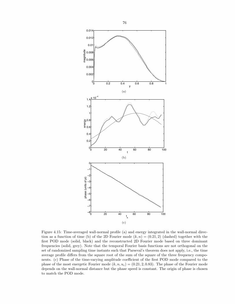
76

0 0.2 0.4 0.6 0.8 10

0.002

0.004

0.006

0.008

0.01

0.012

0.014

ymagnitude

(a)

0 20 40 60 80 1000

0.2

0.4

0.6

0.8

1

1.2

1.4x 10−4

t

ener

gy

(b)

0 20 40 60 80 100−8

−7

−6

−5

−4

−3

−2

−1

0

ts

phas

e (u

nits

of p

i)

(c)

Figure 4.15: Time-averaged wall-normal profile (a) and energy integrated in the wall-normal direc-tion as a function of time (b) of the 2D Fourier mode (k, n) = (0.21, 2) (dashed) together with thefirst POD mode (solid, black) and the reconstructed 2D Fourier mode based on three dominantfrequencies (solid, grey). Note that the temporal Fourier basis functions are not orthogonal on theset of randomized sampling time instants such that Parseval’s theorem does not apply, i.e., the timeaverage profile differs from the square root of the sum of the square of the three frequency compo-nents. (c) Phase of the time-varying amplitude coefficient of the first POD mode compared to thephase of the most energetic Fourier mode (k, n, uc) = (0.21, 2, 0.83). The phase of the Fourier modedepends on the wall-normal distance but the phase speed is constant. The origin of phase is chosento match the POD mode.

77

Duggleby et al. (2007) Present StudyRe 4,300 24,580R+ 150 685L 20R 30RTs 5000 100DOF 2.6× 106 31× 106

Nmodes 2763 8700Decomposition (k, n, q) (k, n, uc, q)

Table 4.2: Comparison of the parameters for the Duggleby et al. (2007) POD analysis and thepresent modal decomposition including the sampling duration Ts, the number of degrees of freedomDOF (grid points) used to compute the modes, and the number of modes Nmodes required to capture90% of the TKE / u′2 for the two analyses, respectively. The last row indicates the order of thesuccessive decompositions performed on the data.

capture more than 90% of the 2D Fourier mode energy, compared to one POD mode. However, the

magnitude of each propagating wave, resulting from the modal decomposition, is constant, whereas

the magnitude of the POD coefficients varies in time, in a non-simple way, due to the finite-time

averaging. When the sampling duration tends to infinity, the coefficients of the POD modes should

converge to the temporal Fourier modes obtained by compressive sampling, because the flow is

statistically steady (Berkooz et al., 1993).

The time evolution of the streamwise turbulence intensity, contained in the reconstructed 2D

Fourier mode (0.21, 2) based on the three propagating waves, obtained by integrating the square

of the amplitude in the wall-normal direction, is plotted on figure 4.15(b), and compared to the

magnitude squared of the first POD mode. The smoother time-variation of the reconstructed mode

is a consequence of the truncation of the Fourier series representation in time after the third-most

energetic mode, i.e., the use of three sparse frequencies and neglect of other, significantly less ener-

getic frequencies. The phase speed of the first POD mode is shown on figure 4.15(c) and matches the

convection velocity of the most energetic propagating wave (0.21, 2, 0.83). We observed that there is

a definite period to the DNS 2D Fourier mode and POD mode variations corresponding to an am-

plitude modulation of the signal at the same timescale as the one visualized on figure 4.8. However,

for other 2D Fourier modes, the timescale of the first POD mode amplitude variations differs from

the period of the Fourier mode. Although the POD and the propagating wave decomposition both

converge, they do so in different ways.

The POD analysis of turbulent pipe flow DNS data by Duggleby et al. (2007) required 2763

(k, n, q) modes to capture 90% of the turbulent kinetic energy (TKE) at a significantly lower Reynolds

number of 4300 and over a domain length of 20R, as opposed to 8700 2D Fourier modes in the present

decomposition. The relevant parameters for the two decompositions are summarized in table 4.2.

These two decompositions showed that the low (k, n) modes are the most energetic and are also

tall in the wall-normal direction. Among the POD modes computed by Duggleby et al. (2007), the

modes with q = 1, i.e., with no zero crossing, are the most energetic. Similarly, in the present

78

decomposition, about 40% to 50% of the energy is contained in the first singular mode with no zero

crossing.

The time-varying POD coefficients need to be extracted from the data and saved at every sam-

pling time instant, whereas for the propagating waves, only their relative magnitude and phase

need to be saved. In addition, the flow decomposition as a superposition of propagating waves with

model-based radial basis functions provides a link between the flow structures and the governing

equations, described in the next section, allowing, for example, for the identification of the dominant

amplification mechanisms sustaining the waves.

4.4 Discussion

The preceding section contained observations concerning the decomposition of real DNS velocity

fields, using appropriate bases in all four dimensions. In this section, we advance the analytical

treatment of the NS equations, in order to identify physical mechanisms sustaining different classes

of modes, which can be identified as propagating waves with a radial amplitude variation. More

precisely, we investigate the relative importance of non-normality and criticality on the amplification

of the propagating waves, as a function of their streamwise wavenumber and mode order, and the

contraints imposed by the dominant amplification mechanisms on the radial extent of the waves.

4.4.1 Componentwise Form of the Input-Output Relationship

The input-output relationship formulated by McKeon & Sharma (2010) (equation (4.16)) can be

expanded to give

crk,n,ω

cθk,n,ω

cxk,n,ω

= R

frk,n,ω

fθk,n,ω

fxk,n,ω

, (4.32)

where

R =

Re T1(D + C + r−2)−1 Re T1(D + C + r−2)−1B(D + C + r−2)−1 0

−Re T1(D + C + r−2)−1B(D + C + r−2)−1 Re T1(D + C + r−2)−1 0

−Re2(D + C)−1DU T2(D + C + r−2)B−1 −Re2(D + C)−1DU T2 Re(D + C)−1

,

(4.33)

79

and

T1 = (I + (D + C + r−2)−1B(D + C + r−2)−1B)−1, (4.34)

T2 = (B + (D + C + r−2)B−1(D + C + r−2))−1, (4.35)

B = 2inr−2, (4.36)

C = iRe(ω − kU), (4.37)

D = −∂rr − r−1∂r + n2r−2 + k2, (4.38)

where I is the identity operator. Here, D is the Laplacian in cylindrical coordinates and can be

interpreted as a dissipation term whose action is proportional to k2 and to the curvature in the radial

direction. Therefore, the action of D is large for modes that are short in the streamwise and radial

directions (as opposed to spanning the whole radius). Phenomena associated with the existence of a

critical layer are captured by C, henceforth the criticality term, which vanishes at the critical layer.

Clearly, the norm of R will be large, corresponding to large amplification of input disturbances,

fk,n,ω(r), if both C and D are small. We investigate here the influence of these two terms on the

output from the SVD. In the analysis that follows, the azimuthal wavenumber is set to n = 3, an

energetically dominant azimuthal wavenumber in the DNS (see table 4.1), in order to make B a

function only of radius.

In order to quantify the distribution of forcing between the radial, streamwise and azimuthal

directions, we introduce the forcing energy (correctly the forcing power per unit time), PFk,n,ω,q,

defined as

PFk,n,ω,q =

∫ 1

0

fk,n,ω,q(r)f∗k,n,ω,q(r)rdr = 1, (4.39)

and the streamwise

PF xk,n,ω,q =

∫ 1

0

fxk,n,ω,q(r)fx∗k,n,ω,q(r)rdr, (4.40)

and azimuthal

PF θk,n,ω,q =

∫ 1

0

fθk,n,ω,q(r)fθ∗k,n,ω,q(r)rdr, (4.41)

contributions to the forcing energy PFk,n,ω,q. The radial contribution to PFk,n,ω,q is given by

1−PF xk,n,ω,q−PF θk,n,ω,q and is always low, for the range of streamwise and azimuthal wavenumbers

considered in this study.

The dependence of the spatial distribution of the forcing and response energy on streamwise

wavenumber and singular mode order, (k, q), is considered on figure 4.16, for constant azimuthal

wavenumber and convection velocity (n = 3 and uc = 0.8, representative of the range observed in

the DNS data). The contours of the streamwise and azimuthal contributions to the forcing and

response energy are plotted as a function of the streamwise wavenumber and singular mode order.

80

k

q

10−1 100 101

2

4

6

8

10

12

14

0

0.2

0.4

0.6

0.8

1

(a)

k

q

10−1 100 101

2

4

6

8

10

12

14

0

0.2

0.4

0.6

0.8

1

(b)

k

q

10−1 100 101

2

4

6

8

10

12

14

0

0.2

0.4

0.6

0.8

1

(c)

k

q

10−1 100 101

2

4

6

8

10

12

14

0

0.2

0.4

0.6

0.8

1

(d)

Figure 4.16: Streamwise (a),(c) and azimuthal (b),(d) contributions to the forcing (top row) andresponse (bottom row) energy, as a function of the streamwise wavenumber and singular mode order,in the presence of mean shear and for n = 3, uc = 0.8.

81

k

Uc

10−2 10−1 100 101

0.5

0.6

0.7

0.8

0.9

1

0.2

0.4

0.6

0.8

Figure 4.17: Cross-sectional contribution to the forcing energy for the first singular mode and withn = 3. The preferential forcing direction switches from being mainly in the cross-sectional planeat low k to being mainly streamwise at high k at a value of k around 4 – 5 corresponding to thestreamwise length of the near-wall type structures (k = 4.3 corresponds to 1, 000 viscous lengthunits at Re = 24, 580).

(Recall from equation (4.19) that the normalization requires that the sum over all cross-stream and

streamwise directions, i.e., PFk,n,ω,q, is equal to 1.) The alternating preference for streamwise and

azimuthal forcing and response modes at high k is a consequence of the oblique propagation of the

individual propagating waves.

For the first singular mode and for k ≤ 4 − 5, the forcing is predominantly in the azimuthal

direction and the response in the streamwise direction. The same observation applies to all singular

modes of order 1 – 15, for k ≤ 1, but the cross-stream contribution to the forcing energy decreases

with the singular mode order. For k ≥ 1, the first singular mode exhibits a forcing mainly in

the streamwise direction, and a predominant response in the azimuthal direction; for higher-order

singular modes, the SVD tends to favor either a forcing and response in the streamwise direction,

or a forcing and response in the azimuthal direction. The selection of the same dominant spatial

direction for both the forcing and the response by the SVD at high k is a characteristic typical of a

normal system. The contours of the forcing and response energy are qualitatively similar for other

azimuthal wavenumbers and convection velocities.

Figure 4.17 shows isocontours of the cross-stream contribution to PFk,n,ω,q for the first singular

mode, q = 1, as a function of streamwise wavenumber and convection velocity, (k, uc). At low

streamwise wavenumber, k ≤ 1, more than 80% of the forcing energy is in the cross-sectional

plane, relatively independent of convection velocity, and figure 4.16 shows that the response is

predominantly in the streamwise direction. For k ≥ 4 − 5, which corresponds to the wavelength of

the near-wall type structures (λ+ = 1000) at this Reynolds number, more than 50% of the forcing

energy is in the streamwise direction, and the response is also predominantly in the streamwise

direction.

82

Jovanovic & Bamieh (2005) studied a similar componentwise energy amplification in channel

flows, and found amplification proportional to Re3 for forcing in the cross-sectional plane, resulting

in a response in the streamwise velocity component. This large amplification was shown to be at-

tributable to the non-normality of the linear operator governing the flow, arising from the coupling

between forcing in the cross-sectional plane and the streamwise velocity component via the mean

shear. All the other combinations of forcing and response directions were shown to lead to ampli-

fication proportional to the Reynolds number, as is typical of a normal system (Farrell & Ioannou,

1993).

While the Reynolds number scaling of the first singular modes has not been investigated explicitly,

the results presented here appear to be in accordance with the results of Jovanovic & Bamieh (2005).

The predominance of the azimuthal contribution to the forcing energy PF θk,n,ω,q at low k observed in

figure 4.16 is also supported by the results of Jovanovic & Bamieh (2005) showing that streamwise-

constant near-wall excitation in the spanwise direction has by far the strongest effect on the flow.

4.4.2 Influence of Non-Normality on Disturbance Amplification

Kim & Lim (2000) performed a DNS of turbulent channel flow with and without the linear term

coupling the wall-normal velocity to the wall-normal vorticity, which is responsible for the non-

normality of the underlying operator. Those authors showed that decoupling the evolution of the

wall-normal vorticity from the evolution of the wall-normal velocity results in the decay of turbulent

fluctuations, with the implication that non-normality is necessary (but not sufficient) to maintain

turbulence. In this work, decoupling of the streamwise velocity fluctuations from cross-stream forcing

(by canceling the mean shear) was used to quantify the influence of non-normality on the system

amplification and on the selection of the preferential forcing and response directions by the SVD.

When the coupling is suppressed (zeroed) and there is little forcing in the radial direction, the

resolvent formulation of equation (4.32) simplifies to

cxk,n,ω = Re(D + C)−1fxk,n,ω, (4.42)

cθk,n,ω = Re (I + (D + C + r−2)−1B(D + C + r−2)−1B)−1 (D + C + r−2)−1 fθk,n,ω, (4.43)

for the streamwise and azimuthal velocity components, respectively. Under these conditions, denoted

the “decoupled system,” forcing in either the streamwise or azimuthal directions can only generate

a response in the same direction.

The singular value as a function of the singular mode order at three different streamwise wavenum-

bers is plotted on figure 4.18 for the coupled and decoupled (effectively non-normal and normal)

systems.

83

0 10 20 30 40 5010−1

100

101

102

103

104

q

sigm

a q

(a)

0 10 20 30 40 50100

101

102

103

104

105

q

sigm

a q

(b)

Figure 4.18: Amplification as a function of the singular mode order with (solid) and without (dashed)the linear coupling term for the modes (k, n, uc) = (k, 3, 0.5) (a) and (k, n, uc) = (k, 3, 0.8) (b)for three different streamwise wavenumbers k = 0.1, 1, 10. The arrow indicates the direction ofincreasing k.

84

k

q

10−1 100 101

2

4

6

8

10

12

14

0

0.2

0.4

0.6

0.8

1

(a)

k

q

10−1 100 101

2

4

6

8

10

12

14

0

0.2

0.4

0.6

0.8

1

(b)

k

q

10−1 100 101

2

4

6

8

10

12

14

0

0.2

0.4

0.6

0.8

1

(c)

k

q

10−1 100 101

2

4

6

8

10

12

14

0

0.2

0.4

0.6

0.8

1

(d)

Figure 4.19: Streamwise (a),(c) and azimuthal (b),(d) contributions to the forcing (top row) andresponse (bottom row) energy, as a function of the streamwise wavenumber and singular mode order,in the absence of mean shear and for n = 3, uc = 0.8.

Any difference is concentrated in the first few singular values for k = 1, 10, while significantly

larger amplification is obtained when non-normality effects are present for the first few singular

modes at low streamwise wavenumber k ≤ 1. The amplification gain due to the non-normality

varies from a factor 2 – 3 at k = 10 and uc = 0.5 to two orders of magnitude at k = 0.1 and

uc = 0.8. For a range of higher-order modes at k = 0.1, however, the singular values for the

decoupled system are larger than for the coupled case.

The contours of the streamwise and azimuthal contributions to the forcing and response energy,

corresponding to this decoupled system, are plotted as a function of the streamwise wavenumber and

singular mode order in figure 4.19. A comparison with the results from the fully coupled resolvent

of figure 4.16 shows that any differences attributable to removing the source of non-normality are

concentrated in the low-k modes, with the exception of the first singular modes. The first singular

modes have a response predominantly in the azimuthal direction at high k for both the coupled and

decoupled systems, implying that, for the streamwise velocity component, non-normality effects are

85

0 0.2 0.4 0.6 0.8 10

0.5

1

1.5

2

2.5

3

3.5

4

y

mag

nitu

de

(a)

0 0.2 0.4 0.6 0.8 10

0.5

1

1.5

2

2.5

3

3.5

4

y

mag

nitu

de

(b)

Figure 4.20: Magnitude of the streamwise velocity component of the singular mode with 5 localpeaks for the Fourier modes (k, n, uc) = (1, 3, 0.5) (a) and (k, n, uc) = (1, 3, 0.8) (b) with (solid) andwithout (dashed) non-normality effects. The modes have a significantly different shape even thoughthe amplification is the same with or without mean shear for these modes at k = 1. The order ofthe singular mode with five local peaks from SVD of the coupled and uncoupled resolvent is q = 5and q = 9, respectively.

only important at low k, regardless of the mode order.

In addition to enhancing the amplification associated with the normal operator, non-normality

effects also result in the broadening of the mode shapes, as can be seen in figure 4.20, comparing the

streamwise singular modes (k, n, uc, q) = (1, 3, 0.5, 0.8, 5) and (k, n, uc, q) = (1, 3, 0.5, 0.8, 9) obtained

from SVD of the coupled and uncoupled resolvents, respectively. The mode order was chosen such

that all the singular modes have 5 local peaks.

Equation (4.32) shows that the response in the streamwise direction is proportional to D−3 for

azimuthal forcing and D−1 for streamwise forcing, implying that modes for which a non-normal

mechanism contributes significantly to the amplification will be associated with small D, or small

curvature in the radial direction, namely modes that are tall in the wall-normal direction, in agree-

ment with the radial variation of the long, globally energetic modes characterized in the previous

section.

4.4.3 Influence of Criticality on Disturbance Amplification for High k

Modes

The previous subsection showed that there is little difference between the coupled and decoupled

system response for relatively high k modes, implying that the decoupled resolvent can be used to

study the high k modes. In this case, the flow is purely convective, i.e., depends on the mean velocity

profile U(y), but not on the mean shear dUdy , and the resolvent (equation (4.32)) simplifies to

cxk,n,ω = Re(D + C)−1fxk,n,ω, (4.44)

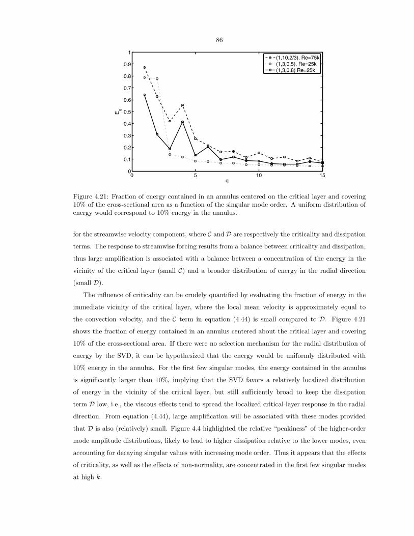
86

0 5 10 150

0.1

0.2

0.3

0.4

0.5

0.6

0.7

0.8

0.9

1

q

E q

(1,10,2/3), Re=75k(1,3,0.5), Re=25k(1,3,0.8) Re=25k

Figure 4.21: Fraction of energy contained in an annulus centered on the critical layer and covering10% of the cross-sectional area as a function of the singular mode order. A uniform distribution ofenergy would correspond to 10% energy in the annulus.

for the streamwise velocity component, where C and D are respectively the criticality and dissipation

terms. The response to streamwise forcing results from a balance between criticality and dissipation,

thus large amplification is associated with a balance between a concentration of the energy in the

vicinity of the critical layer (small C) and a broader distribution of energy in the radial direction

(small D).

The influence of criticality can be crudely quantified by evaluating the fraction of energy in the

immediate vicinity of the critical layer, where the local mean velocity is approximately equal to

the convection velocity, and the C term in equation (4.44) is small compared to D. Figure 4.21

shows the fraction of energy contained in an annulus centered about the critical layer and covering

10% of the cross-sectional area. If there were no selection mechanism for the radial distribution of

energy by the SVD, it can be hypothesized that the energy would be uniformly distributed with

10% energy in the annulus. For the first few singular modes, the energy contained in the annulus

is significantly larger than 10%, implying that the SVD favors a relatively localized distribution

of energy in the vicinity of the critical layer, but still sufficiently broad to keep the dissipation

term D low, i.e., the viscous effects tend to spread the localized critical-layer response in the radial

direction. From equation (4.44), large amplification will be associated with these modes provided

that D is also (relatively) small. Figure 4.4 highlighted the relative “peakiness” of the higher-order

mode amplitude distributions, likely to lead to higher dissipation relative to the lower modes, even

accounting for decaying singular values with increasing mode order. Thus it appears that the effects

of criticality, as well as the effects of non-normality, are concentrated in the first few singular modes

at high k.

87

The concentration of both criticality and non-normality effects in the first few singular modes

helps to explain the sharp decrease in singular values between the first mode and the higher-order

singular modes shown in figure 4.18. This drop-off occurs faster than for the projection coefficients

Pq (defined by equation (4.28)) computed for the long streamwise waves extracted from the DNS

data, such that the amount of forcing increases with the singular mode order for the k ∼ 1 modes.

Under white noise forcing, the higher-order singular modes have low (negligible) magnitude com-

pared to the first few singular modes, due to the sharp decrease in singular values. In the DNS,

however, the presence of higher-order singular modes containing a finite amount of energy implies

that the nonlinear interactions result in a nonuniform distribution of forcing among the singular

modes, characterized by increasing forcing energy with mode order. One possible explanation is

that the nonlinear interaction of the first few (highly amplified) singular modes provides such forc-

ing distribution, implying that the higher-order singular modes are a residual of that nonlinear

interaction capturing the energy distribution in the wall-normal direction away from the critical-

layer. Figure 4.22 illustrates how the DNS mode (0.84, 3, 0.83), representative of the k ∼ 1 modes,

is decomposed into a component corresponding to the first three singular modes, which are highly

amplified, and a residual containing energy mainly away from the critical layer, and corresponding to

the less-amplified higher-order singular modes. The singular modes of order larger than three each

contain less than 2% of the DNS propagating wave energy, justifying a cutoff between the optimal

and residual modes after the third mode.

A cartoon of the dominant amplification mechanisms as a function of the streamwise wavenumber

and singular mode order for (n, uc) = (3, 0.8) is shown in figure 4.23, superposed onto the contours

of the singular value on a logarithmic scale. At low streamwise wavenumber, large amplification

is due to non-normality (regions 1 and 2), with a boost from criticality at low mode order (region

2). At high streamwise wavenumber, criticality effects are concentrated in the first few singular

modes (region 3) and result in the large amplification of these low-order modes. The higher-order

modes experience a relatively low amplification inversely proportional to the viscosity, as is the

case for a normal system (region 4). The line delimiting the region where non-normality effects are

important follows the contours of the singular value, indicating that the amplification is significantly

larger in the presence of non-normality effects. For the smaller structures, inspection of the resolvent

(equation (4.32)) shows that, as the streamwise wavenumber increases, the amplification due to non-

normality decreases at least as k−4, and the only source of large amplification is criticality. This

change in the dominant amplification mechanism is reflected in the change in the preferential forcing

direction from cross-sectional to streamwise for k between 4 and 5, depending on the convection

velocity (see figure 4.17) and has implications on the modeling of the smaller-scale structures that

will be discussed in the next subsection.

88

0 0.2 0.4 0.6 0.8 10

1

2

3

4

x 10−3

y

mag

nitu

de

(a)

0 0.2 0.4 0.6 0.8 10

1

2

3

4

5

6x 10−3

y

mag

nitu

de

(b)

0 0.2 0.4 0.6 0.8 10

0.5

1

1.5

2x 10−3

y

mag

nitu

de

(c)

Figure 4.22: Wall-normal profile of (a) the DNS propagating wave (k, n, uc) = (0.84, 3, 0.83), (b)decomposed into the first three singular modes with (dashed) and without (solid) non-normalityeffects and (c) a residual containing energy mainly away from the critical layer, and correspondingto the higher-order singular modes.

89

k

q

10−1

100

101

0.5

1

1.5

2

2.5

3

3.5

1

3 2

4

Figure 4.23: Schematic of the regions where non-normality effects (1 and 2) and criticality effects(2 and 3) are important on top of the contours of the singular value on a logarithmic scale, asa function of the streamwise wavenumber and singular mode order at (n, uc) = (3, 0.8). The linedelimiting the region where non-normality effects are important (regions 1 and 2) follows the contoursof the singular value, indicating that the amplification is significantly larger in the presence of non-normality effects. In region 4, the amplification is relatively low and inversely proportional to theviscosity as is the case for a normal system.

90

4.4.4 Implications of the Present Study on Analyses on Criticality and

Non-Normality

The analysis of the resolvent given above indicated a change in the dominant amplification mecha-

nism from non-normality to criticality with increasing k, suggesting that the smaller structures are

more localized in the wall-normal direction about the critical layer, as opposed to the large-scale

structures spanning the whole radius. The smaller structures are expected to be well represented by

the first singular mode which captures most of the criticality effects at high k. Figure 4.25 shows

that the width of the first singular mode decreases with k and increases with uc, such that the

smaller structures are getting increasingly narrower in the wall-normal direction as they shorten in

the streamwise direction or are located closer to the wall.

To quantify the radial extent of the small structures, the scaling of the first singular mode width

with k and uc is considered by defining the thickness, ε, as the mode width at 50% peak magnitude.

ε depends on both k and uc for a given Reynolds number. Figure 4.24(a) shows the thickness of

the first singular mode as a function of k at uc = 23 and n = 3, compared to the scaling law k−α

with α = 13 ,

12 . The value of α representing best the data varies from 1

3 to 12 depending on uc and

equals 12 at uc = 2

3 . The dependence of the first singular mode thickness on the mean shear at the

critical layer is evaluated by varying the convection velocity from 0.5 to 0.95 by increments of 0.05

(thereby effectively displacing the critical layer away from the wall to a region where the mean shear

is lower as uc is increased). The width of the first singular mode for the various convection velocities

is plotted on figure 4.24(b) and is well represented by a line proportional to U′− 1

3crit , where U ′crit is the

mean shear at the critical layer.

Under the classical critical-layer analysis in Cartesian coordinates, e.g., Schmid & Henningson

(2001), the Orr-Sommerfeld (OS) equation simplifies to an Airy equation in the vicinity of the critical

layer, leading to an analytical scaling of the internal layer thickness as (kReU ′crit)− 1

3 . The internal

layer is defined as the region around the critical layer where viscous effects need to be introduced

to regularize the solution to the inviscid OS equation. While this analysis does not have a direct

analytical analog in the cylindrical coordinates of pipe flow, because the OS and Squire equations

are fully coupled, interestingly the upper bound on the exponent obtained for the scaling of the

first singular mode thickness as a function of the streamwise wavenumber, and the exponent for the

scaling with the mean shear at the critical layer, correspond to the classical − 13 exponent, suggesting

at least a phenomenological similarity between coordinate systems.

The analysis of the resolvent presented in this chapter indicated that the small scales are localized

in the vicinity of the critical-layer, and thus exhibit amplification with a large contribution from

criticality. Experimental measurements have confirmed the wall-normal localization of the small

scales near the critical-layer, or equivalently, that the short scales convect at the local mean velocity.

91

100 101

10−1

k

epsilon

(a)

100 101

10−1

u’crit

epsilon

(b)

Figure 4.24: Thickness of the first singular mode as a function of the streamwise wavenumber k atuc = 2

3 and n = 3 (a) and as a function of the mean shear at the critical layer U ′crit for uc varyingfrom 0.5 to 0.95 by increments of 0.05 at k = 1 and n = 3. The dots indicate the data points, the

solid and dashed lines correspond to the scaling laws k−13 and k−

12 (a), respectively, and U

′− 13

crit (b).

92

0 0.1 0.2 0.3 0.4 0.5 0.6 0.7 0.8 0.9 10

0.5

1

1.5

2

2.5

3

3.5

y

magnitude

(a)

0 0.1 0.2 0.3 0.4 0.5 0.6 0.7 0.8 0.9 10

0.5

1

1.5

2

2.5

3

3.5

4

4.5

5

y

magnitude

(b)

Figure 4.25: Wall-normal profile of the first singular modes (k, n, uc) = (1 : 2 : 8, 3, 23 ) (a) and

(k, n, uc) = (1, 3, 0.5 : 0.1 : 0.9) (b). The arrow indicates the direction of increasing k (a) and uc (b).

93

The present analysis highlights that the small scales are well described by criticality-based studies,

such as the approach of McKeon & Sharma (2010), due to the negligible importance of non-normality

effects at high k shown on figure 4.18, and the strengthening of the spatial localization of the small

scales around the critical-layer with increasing k (figure 4.25).

Experimental measurements have also shown that the long streamwise structures extend from

the wall to the core of the pipe, and convect at a speed characteristic of the log region (LeHew

et al., 2011). These large scales are the ones captured in the present modal decomposition of the

DNS due to their significant contribution to the radial-integrated streamwise turbulence intensity.

In accordance with the experimental measurements and the modal decomposition of turbulent pipe

flow DNS data, the low k propagating waves were shown, by the analysis of the resolvent presented

here, to span the whole radius, i.e., to be tall in the wall-normal direction; as the decrease in

curvature associated with the stretching of the modes in the wall-normal direction results in lower

viscous dissipation. Due to their large radial extent, as shown on figure 4.8, these propagating waves

are relatively insensitive to criticality effects, and are therefore best described by globally optimal,

linear, studies of the NS equations, e.g., Schmid & Henningson (1994).

The concentration of the influence of non-normality effects in the low streamwise wavenumber,

low-order modes is consistent with the classical picture of the energy cascade: the extraction of energy

from the mean flow by the large scales (due to the non-normality of the underlying operator), transfer

of energy from the large to the small scales by the triadic (nonlinear) interactions, and dissipation

by the small scales. Further progress on the spectral transfer and spatial transport of energy is likely

possible using the simplified form of the resolvent given in equation (4.44).

4.5 Summary

A modal decomposition of turbulent pipe flow DNS data at Re = 24, 580, as a sum of propagating

waves with model-based radial basis functions, was presented to obtain sparse representations of the

flow that are coherent in the wall-normal direction, and to provide a link between the propagat-

ing waves and the governing equations, allowing for the identification of the physical mechanisms

sustaining the waves.

The data requirements to perform the modal decomposition were significantly reduced by the

use of compressive sampling to extract the frequency content of the flow, and by the introduction of

model-based radial basis functions, obtained by following the approach of McKeon & Sharma (2010)

to decompose the turbulent pipe flow resolvent into a set of orthonormal forcing and response modes,

ranked by their amplification. These two approaches made possible an efficient modal decomposition

of turbulent pipe flow in the three spatial directions and in time.

The decomposition of the flow as a sum of propagating waves was explored by McKeon &

94

Sharma (2010), and shown to capture the coherence in the wall-normal direction. The present study

focused on the globally energetic propagating waves contributing largely to the radial-integrated,

time-averaged, streamwise turbulence intensity. These propagating waves were shown to be long in

the streamwise direction and tall in the wall-normal direction.

The modal decomposition is low order, due to the large amount of energy captured by the

globally energetic modes, and requires only 51 2D Fourier modes to capture 20% of the streamwise

turbulence intensity. Each 2D Fourier mode contains no more than 5 sparse frequencies, and for

each frequency about 95% of the energy is captured with less than 12 singular modes in the radial

direction. Altogether, 51×5×12 ≈ 3000 modes are required to capture about 20% of the streamwise

turbulence intensity, compared to the 109 degrees of freedom of the subsampled DNS, illustrating

the significant data compression obtained with the modal decomposition presented in this chapter.

This modal decomposition results in time-invariant amplitude coefficients, highlighting that the

statistical steadiness of the flow is enforced, as opposed to the time-varying coefficients obtained via

POD based on a time average of the velocity cross-correlation tensor.

Analysis of the resolvent led to the identification of the dominant physical mechanisms sustaining

the propagating waves, as a function of their streamwise wavenumber. It was shown that the short

streamwise waves are localized in the vicinity of the critical layer, and amplified by criticality effects,

whereas the long streamwise waves are tall in the wall-normal direction, and have large amplifica-

tion due to non-normality effects, resulting in energy extraction from the mean flow. In Cartesian

coordinates, the standard Orr-Sommerfeld theory also predicts the importance of criticality effects

and the scaling of the internal layer with k.

The resolvent can be seen as a rank one operator at high k in accordance with the predictions of

McKeon & Sharma (2010), based on the sharp decrease in amplification from the first to the second

singular mode, and as a low-rank operator at low k. Criticality analyses are particularly suited

to describe the small scales, since non-normality effects play a minor role compared to criticality.

It was shown in the present study that a value of k around 4 – 5, corresponding to the near-wall

type structures at Re = 24, 580 (λ+ = 1000), constitutes the lower bound on the length of the

modes benefiting mainly from criticality effects. At lower k, the propagating waves are tall in the

wall-normal direction, in order to maximize non-normality effects. These large scales are the ones

captured in the globally optimal studies, and in the present modal decomposition of DNS data, due

to their significant contribution to the radial integrated streamwise turbulence intensity.

95

Chapter 5

Conclusion

Two models of turbulent pipe flow were presented to investigate the physics of turbulence, and to

study the importance of linear non-normal, critical, and nonlinear effects, in wall-bounded turbu-

lence. Analytical progress was made possible by appropriate simplifications of the Navier-Stokes

equations, depending on the phenomena of interest, and by the decomposition of the flow into a

mean component and fluctuations about the mean. Two main features of turbulent pipe flow, i.e.,

the blunting of the velocity profile during transition and the sustenance of the turbulent fluctuations,

were studied in detail. The mechanisms responsible for the blunting of the velocity profile were in-

vestigated by considering a streamwise-constant projection of the Navier-Stokes equations, whereas

the mechanisms sustaining different classes of structures were identified by linear analysis of the

resolvent, using the modeling assumption that the nonlinear terms in the Navier-Stokes equations

act as an unstructured forcing of the linear dynamics.

The main contributions of this thesis to the understanding of the role of linear non-normal,

critical, and nonlinear effects in wall-bounded turbulence are summarized in this chapter. A more

detailed description of the results obtained with each model is given at the end of their respective

chapter.

The non-normal mechanisms are associated with the linear coupling term between the cross-

sectional and streamwise velocity fluctuations, and were shown to result in large amplification of the

cross-stream forcing modes, in both the nonlinear streamwise-constant model and the analysis of the

turbulent pipe flow resolvent. The most amplified response modes, computed with the two models

presented in this thesis, correspond to streamwise streaks of the streamwise velocity fluctuations, in

accordance with the results of Jovanovic & Bamieh (2005). Non-normality effects are prominent at

low streamwise wavenumber and were shown to be maximized if the low streamwise wavenumber

modes were also tall in the wall-normal direction, in order to decrease their viscous dissipation; as

opposed to being localized near the wall, where the shear is higher. This is a new formalization of

the constraints imposed by non-normality on the radial extent of optimally amplified modes.

Criticality effects are associated with the nearly singular behavior of the resolvent at high

96

Reynolds number, when a propagating wave convects at a speed corresponding to the local mean

velocity (at, or close to, the peak magnitude of the wave). Criticality effects result in the large

amplification of propagating waves that are localized near the critical-layer, and were shown in this

thesis to be the dominant amplification mechanisms for the high streamwise wavenumber modes, for

which non-normality effects are negligible; and to constrain the optimally amplified high streamwise

wavenumber modes to be localized in the vicinity of the critical-layer. The work in this thesis allows

the reconciliation of the well-known results (Bamieh & Dahleh, 2001; Jovanovic & Bamieh, 2005;

Schmid & Henningson, 1994) concerning optimal disturbance amplification due to non-normal effects

with the recent resolvent analysis of McKeon & Sharma (2010), which highlighted the importance

of criticality effects.

Nonlinear effects result in the redistribution of the high- and low-speed streaks over the cross-

section of the pipe, and were shown to be required to capture the change in mean flow that occurs

during transition to turbulence. The nonlinear terms convect the streamwise streaks in such a way

that the high-speed streaks concentrate near the wall and the low-speed streaks near the center

of the pipe, thereby causing a blunting of the velocity profile. These mechanisms were discovered

by numerical simulation of the streamwise-constant model under both stochastic and deterministic

forcing of the streamfunction equation.

The two models were shown to capture energetic structures of wall-bounded turbulence, taking

the form of streamwise-elongated rolls and streaks in the streamwise-constant model, and of coher-

ent propagating waves in the model-based modal decomposition of turbulent pipe flow, and were

validated against experimental and numerical data.

A novel application of compressive sampling was presented, to efficiently extract the frequency

content of energetic modes in wall-bounded turbulence. Compressive sampling, together with the use

of radial basis functions obtained by SVD of the resolvent, made possible a full modal decomposition

of turbulent pipe flow, in the three spatial directions and in time, resulting in sparse representations

of the flow. A full modal decomposition of wall-bounded turbulence is not commonly pursued,

due to the significant data requirements to compute statistically-converged, data-based, radial basis

functions.

Future research will involve determining the Reynolds number dependence of the gradual tran-

sition from non-normality to criticality dominated amplification; or evaluating the sensitivity of the

radial basis functions computed by SVD of the resolvent to changes in the input mean velocity pro-

file, in order to couple the resolvent analysis to the streamwise-constant model, and thereby obtain

a data independent framework for the study of wall-bounded turbulence. It also seems possible to

relate the constraints on the radial extent of the modes imposed by the dominant amplification mech-

anisms (non-normality and criticality), described in this thesis, to the spatial flux of scale energy in

the wall-normal direction.

97

Appendix A

Matlab code used to solve theconvex optimization problem

% Nr is the number of grid points in the radial direction

% Ns is the number of samples

% 2D_Fourier(Nr,Ns) is the 2D Fourier mode as a function of the wall-normal

% distance r discretized over Nr points and the Ns number of samples

% (time instant ts)

% F_out(Nr,Nopti) is the output of the minimization corresponding to

% the frequency content as a function of the wall-normal distance.

Nopti=10*Ns; % number of frequencies for the optimization

f=(-Nopti/2+1:1:Nopti/2)/(Nopti/2); % equispaced frequencies for the optimization

C=exp(-1i*2*pi*ts*f); % constraint matrix: output must match input

% at the sampling time instants

for j=1:Nr

cvx_begin

cvx_quiet(true)

variable x(Nopti) complex;

minimize(norm(x,1)); % minimize the sum of the absolute value

% of the temporal Fourier coefficients

subject to

C * x==2D_Fourier(j,:)’;

cvx_end

F_out(j,:)=x;

end.

98

Bibliography

Adrian, R. J. 2007 Vortex organization in wall turbulence. Phys. Fluids 19 (041301).

del Alamo, J. C. & Jimenez, J. 2006 Linear energy amplification in turbulent channels. J. Fluid

Mech. 559, 205–213.

Baltzer, J. R. & Adrian, R. J. 2011 Structure, scaling, and synthesis of proper orthogonal

decomposition modes of inhomogeneous turbulence. Phys. Fluids 23 (1).

Bamieh, B. & Dahleh, M. 2001 Energy amplification in channel flows with stochastic excitation.

Phys. Fluids 13 (11), 3258–3269.

Berkooz, G., Holmes, P. & Lumley, J. L. 1993 The Proper Orthogonal Decomposition in the

analysis of turbulent flows. Annu. Rev. Fluid Mech. 25, 539–575.

Bilinskis, I. 2007 Digital Alias-Free Signal Processing . John Wiley.

Bourguignon, J.-L. & McKeon, B. J. 2011 A streamwise-constant model of turbulent pipe flow.

Phys. Fluids 23 (9).

Candes, E. J., Romberg, J. & Tao, T. 2006 Robust uncertainty principles: Exact signal re-

construction from highly incomplete frequency information. IEEE Trans. Inf. Theory 52 (2),

489–509.

Candes, E. J. & Wakin, M. B. 2008 An introduction to compressive sampling. IEEE Signal

Processing Magazine 25 (2), 21–30.

Canuto, C. 2006 Spectral Methods: Fundamentals in Single Domains. Springer-Verlag.

Chen, S., Donoho, D. L. & Saunders, M. A. 1998 Atomic decomposition by basis pursuit.

SIAM Journal On Scientific Computing 20 (1), 33–61.

Chung, D. & McKeon, B. J. 2010 Large-eddy simulation of large-scale structures in long channel

flow. J. Fluid Mech. 661, 341–364.

Darbyshire, A. G. & Mullin, T. 1995 Transition to turbulence in constant-mass-flux pipe flow.

J. Fluid Mech. 289, 83–114.

99

Dennis, D. & Nickels, T. 2008 On the limitations of Taylor’s hypothesis in constructing long

structures in wall-bounded turbulent flow. J. Fluid Mech. 614, 197–206.

van Doorne, C. W. H. & Westerweel, J. 2009 The flow structure of a puff. Phil. Trans. Royal

Soc. A 367, 489–507.

Duggleby, A., Ball, K. S., Paul, M. R. & Fischer, P. F. 2007 Dynamical eigenfunction

decomposition of turbulent pipe flow. J. Turbulence 8 (43), 1–24.

Duggleby, A., Ball, K. S. & Schwaenen, M. 2009 Structure and dynamics of low Reynolds

number turbulent pipe flow. Phil. Trans. Royal Soc. A 367 (1888), 473–488.

Duguet, Y., Willis, A. P. & Kerswell, R. R. 2010 Slug genesis in cylindrical pipe flow. J.

Fluid Mech. 663, 180–208.

Eckhardt, B. 2007 Turbulence transition in pipe flow. Annu. Rev. Fluid Mech. 39, 447–468.

Eckhardt, B. 2008 Turbulence transition in pipe flow: Some open questions. Nonlinearity 21,

1–11.

Farrell, B. F. & Ioannou, P. J. 1993 Stochastic forcing of the linearized Navier-Stokes equations.

Phys. Fluids 5 (11), 2600–2609.

Gayme, D., McKeon, B. J., Papachristodoulou, A., Bamieh, B. & Doyle, J. C. 2010 A

streamwise constant model of turbulence in plane Couette flow. J. Fluid Mech. 658, 99–119.

George, W. K. & Castillo, L. 1997 Zero-pressure-gradient turbulent boundary layer. Appl.

Mech. Rev. 50, 689–729.

Guala, M., Hommema, S. E. & Adrian, R. J. 2006 Large-scale and very-large-scale motions in

turbulent pipe flow. J. Fluid Mech. 554, 521–542.

Heinrichs, W. 2004 Spectral collocation schemes on the unit disc. J. Comp. Phys. 199 (1), 66–86.

Hellstroem, L. H. O., Sinha, A. & Smits, A. J. 2011 Visualizing the very-large-scale motions

in turbulent pipe flow. Phys. Fluids 23 (1), 703–707.

Hof, B., van Doorne, C. W. H., Westerweel, J., Nieuwstadt, F. T. M., Faisst, H.,

Eckhardt, B., Wedin, H., Kerswell, R. R. & Waleffe, F. 2004 Experimental observation

of nonlinear traveling waves in turbulent pipe flow. Science 305 (5690), 1594–1598.

Hof, B., de Lozar, A., Avila, M., Tu, X. & Schneider, T. M. 2010 Eliminating turbulence

in spatially intermittent flows. Science 327 (5972), 1491–1494.

100

Hoyas, S. & Jimenez, J. 2006 Scaling of velocity fluctuations in turbulent channels up to Reτ =

2003. Phys. Fluids 18.

Hutchins, N. & Marusic, I. 2007 Large-scale influences in near-wall turbulence. Phil. Trans.

Royal Soc. A 365, 647–664.

Hwang, Y. & Cossu, C. 2010 Linear nonnormal energy amplification of harmonic and stochastic

forcing in the turbulent channel flow. J. Fluid Mech. 664, 51–73.

Jimenez, J. & Moser, R. D. 2007 What are we learning from simulating wall turbulence? Phil.

Trans. R. Soc. A 365, 715–732.

Jonsson, I. & Kagstrom, B. 2003 RECSY – A high performance library for Sylvester-type matrix

equations. Euro-Par 2003 Parallel Processing, Proceedings 2790, 810–819.

Joseph, D. D. 1968 Eigenvalue bounds for the Orr-Sommerfeld equation. J. Fluid Mech. 33, 617–

621.

Jovanovic, M. R. & Bamieh, B. 2005 Componentwise energy amplification in channel flows. J.

Fluid Mech. 534, 145–183.

Kim, J. & Lim, J. 1993 A linear process in wall-bounded turbulent shear flows. Phys. Fluids 12 (8),

1885–1888.

Kim, J. & Lim, J. 2000 A linear process in wall-bounded turbulent shear flows. Phys. Fluids 12 (8),

1885–1888.

Kim, K. C. & Adrian, R. J. 1999 Very large-scale motion in the outer layer. Phys. Fluids 11 (2),

417–422.

Kline, S. J., Reynolds, W. C., Schraub, F. A. & Runstadler, P W. 1967 The structure of

turbulent boundary layers. J. Fluid Mech. 30, 741–772.

LeHew, J., Guala, M. & McKeon, B. J. 2011 A study of the three-dimensional spectral energy

distribution in a zero pressure gradient turbulent boundary layer. Expts. in Fluids 51 (4), 997–

1012.

Lindgren, E. R. 1957 The transition process and other phenomena in viscous flow. Arkiv For Fysik

12, 1–169.

Liu, Z., Adrian, R. J. & Hanratty, T. J. 2001 Large-scale modes of turbulent channel flow:

Transport and structure. J. Fluid Mech. 448, 53–80.

Lustig, M., Donoho, D. & Pauly, J. M. 2007 Sparse MRI: The application of compressed

sensing for rapid MR imaging. Magn. Reson. Med. 58 (6), 1182–1195.

101

Marusic, I., McKeon, B. J., Monkewitz, P. A., Nagib, H. M, Smits, A. J. & Sreenivasan,

K. R. 2010 Wall-bounded turbulent flows at high Reynolds numbers: Recent advances and key

issues. Phys. Fluids 22 (6), 1–24.

Maslowe, S. A. 1986 Critical layers in shear flows. Annu. Rev. Fluid Mech. 18, 405–432.

McKeon, B. J. & Sharma, A. 2010 A critical layer framework for turbulent pipe flow. J. Fluid

Mech. 658, 336–382.

Meinhart, C. D. & Adrian, R. J. 1995 On the existence of uniform momentum zones in a

turbulent boundary layer. Phys. Fluids 7 (4), 694–696.

Mellibovsky, F., Meseguer, A., Schneider, T. M. & Eckhardt, B. 2009 Transition in

localized pipe flow turbulence. Phys. Rev. Letters 103.

Meseguer, A. 2003 Streak breakdown instability in pipe Poiseuille flow. Phys. Fluids 15 (5),

1203–1213.

Meseguer, A. & Trefethen, L. N. 2003 Linearized pipe flow to Reynolds number 107. J. Comp.

Phys. 186, 178–197.

Morrison, J. F., McKeon, B. J., Jiang, W. & Smits, A. J. 2004 Scaling of the streamwise

velocity component in turbulent pipe flow. J. Fluid Mech. 1508, 99–131.

Morrison, W. R. B., Bullock, K. J. & Kronauer, R. E. 1971 Experimental evidence of

waves in the sublayer. J. Fluid Mech. 47, 639–656.

Nishi, M., Uensal, B., Durst, F. & Biswas, G. 2008 Laminar-to-turbulent transition of pipe

flows through puffs and slugs. J. Fluid Mech. 614, 425–446.

Papachristodoulou, A. 2005 Scalable analysis of nonlinear systems using convex optimization.

PhD thesis, California Institute of Technology.

Peyret, R. 2002 Spectral methods for incompressible viscous flow , Applied mathematical sciences,

vol. 148. Springer.

Reddy, S. C. & Ioannou, P. J. 2000 Energy transfer analysis of turbulent plane Couette flow.

Proceedings of the IUTAM Laminar-Turbulent Transition pp. 211–216.

Reshotko, E & Tumin, A 2001 Spatial theory of optimal disturbances in a circular pipe flow.

Phys. Fluids 13 (4), 991–996.

Robinson, S. K. 1991 Coherent motions in the turbulent boundary layer. Annu. Rev. Fluid Mech.

23, 601–639.

102

Salwen, H., Cotton, F. W. & Grosch, C. E. 1980 Linear stability of Poiseuille flow in a

circular pipe. J. Fluid Mech. 98, 273–284.

Schmid, P. J. 2000 Linear stability theory and bypass transition in shear flows. Phys. Plasmas 7,

1788–1794.

Schmid, P. J. & Henningson, D. S. 1994 Optimal energy density growth in Hagen-Poiseuille

flow. J. Fluid Mech. 277, 197–225.

Schmid, P. J. & Henningson, D. S. 2001 Stability and Transition in Shear Flows, Applied

Mathematical Sciences, vol. 142. Springer.

Schneider, T. M., Eckhardt, B. & Yorke, J. A. 2007 Turbulence transition and the edge of

chaos in pipe flow. Phys. Rev. Letters 99 (3).

Schoppa, W. & Hussain, F. 2002 Coherent structure generation in near-wall turbulence. J. Fluid

Mech. 453, 57–108.

Shimizu, M. & Kida, S. 2009 A driving mechanism of a turbulent puff in pipe flow. Fluid Dynam.

Res. 41.

Smits, A. J., McKeon, B. J. & Marusic, I. 2011 High Reynolds number wall turbulence. Annu.

Rev. Fluid Mech. 43, 353–375.

Spalart, P. R., Moser, R. D. & Rogers, M. M. 1991 Spectral methods for the Navier-Stokes

equations with one infinite and two periodic directions. J. Comp. Phys. 96 (2), 297–324.

Swanson, C. J., Julian, B., Ihas, G. G. & Donnelly, R. J. 2002 Pipe flow measurements

over a wide range of Reynolds numbers using liquid helium and various gases. J. Fluid Mech. 461,

51–60.

Theodorsen, T. 1952 Mechanism of turbulence. In Proc. 2nd Midwestern Conf. on Fluid Mech.,

pp. 1–19. Ohio State University, Columbus, Ohio.

den Toonder, J. M. J. & Nieuwstadt, F. T. M. 1997 Reynolds number effects in a turbulent

pipe flow for low to moderate Re. Phys. Fluids 9 (11), 3398–3409.

Trefethen, L. N. & Embree, M. 2005 Spectra and Pseudospectra: The Behavior of Nonnormal

Matrices and Operators. Princeton University Press.

Tropp, J. A., Laska, J. N., Duarte, M. F., Romberg, J. K. & Baraniuk, R. G. 2010 Beyond

Nyquist: Efficient sampling of sparse bandlimited signals. IEEE Trans. Inf. Theory 56 (1), 520–

544.

103

Waleffe, F. 1997 On a self-sustaining process in shear flows. Phys. Fluids 9 (4), 883–900.

Wu, X. & Moin, P. 2008 A direct numerical simulation study on the mean velocity characteristics

in turbulent pipe flow. J. Fluid Mech. 608, 81–112.

Wygnanski, I. J. & Champagne, F. H. 1973 On transition in a pipe. Part 1: The origin of puffs

and slugs and the flow in a turbulent slug. J. Fluid Mech. 59, 281–335.

Zikanov, O. Y. 1996 On the instability of pipe Poiseuille flow. Phys. Fluids 8 (11), 2923–2932.