A system for simple real-time anastomotic - iMED...
16
1 A system for simple real-time anastomotic failure detection and wireless blood flow monitoring in the lower limbs Michael A. Rothfuss, Nicholas G. Franconi, Jignesh V. Unadkat, Michael L. Gimbel, Alexander Star, Marlin H. Mickle, Ervin Sejdi´ c Abstract—Current totally implantable wireless blood flow monitors are large and cannot operate alongside nearby monitors. To alleviate the problems with the current monitors, we developed a system to monitor blood flow wirelessly, with a simple and easily interpretable real- time output. To the authors’ knowledge, the implanted electronics are the smallest in reported literature, which reduces bio-burden. Calibration was performed across realistic physiological flow ranges using a syringe pump. The device’s sensors connected directly to the bilateral femoral veins of swine. For one minute each, Blood flow was monitored, then an occlusion was introduced, and then the occlusion was removed to resume flow. Each vein of four pigs was monitored four times, totaling 32 data collections. The implant measured 1.70 cm 3 without battery/encapsulation. Across its calibrated range, includ- ing equipment tolerances, the relative error is less than ±5% above 8.00 mL/min and between -0.8% to +1.2% at its largest calibrated flow rate, which to the authors’ knowledge is the lowest reported in literature across the measured calibration range. The average standard devi- ation of the flow waveform amplitude was three times greater than that of no-flow. Establishing the relative amplitude for the flow and no-flow waveforms was found necessary, particularly for noise modulated Doppler signals. Its size and accuracy, compared with other microcontroller- equipped totally implantable monitors, make it a good candidate for future tether-free free flap monitoring studies. Keywords: anastomosis, bedside monitor, blood flow monitor, continuous wave, Doppler, flowmeter, free flap I. I NTRODUCTION Microvascular free tissue transfer (i.e., free flap) refers to a class of procedures used for reconstructing anatomic Michael A. Rothfuss, Nicholas G. Franconi, Marlin H. Mickle, and Ervin Sejdi´ c are with the Department of Electrical and Computer Engineering, Swanson School of Engineering, University of Pitts- burgh, Pittsburgh, PA, USA. E-mails: [email protected], [email protected], [email protected]. Corresponding author: Ervin Ervin Sejdi´ c: ese- [email protected]. Jignesh V. Unadkat and Michael L. Gimbel are with the Department of Plastic Surgery, University of Pittsburgh, Pittsburgh, PA, USA. E- mails: [email protected], [email protected]. Alexander Star is with the Department of Chemistry, University of Pittsburgh, Pittsburgh, PA, USA. E-mail: [email protected]. defects [1–4], often due to cancer treatment [5], [6], infection, or trauma [7], [8]. These procedures involve the transfer of a block of tissue (i.e., flap) from a donor site (e.g., abdomen, leg) to reconstruct a major defect in another region of the body (e.g., breast, mandible) [9], [10]. Different from simple skin grafting [11], this transfer requires microsurgical connections (anastomoses [12–14]) of veins and arteries to be established be- tween the flap and the new site [15]. Unfortunately, blood vessel patency (i.e., openness of a vessel) can be compromised in up to 10% of cases in the first several days after surgery [16], [17]. This is largely due to vessel thrombosis, compression, kinking, or tension, which creates a surgical emergency, because the trans- ferred flap will fail unless blood flow is reestablished promptly [18–20]. Flap failure results in increased cost [21], patient morbidity [22], [23], and even death [11], [24]. As a result, reconstructive plastic surgeons maintain a low threshold for returning to the operating room to investigate a suspected vascular problem, resulting in an undesired, but accepted, risk of negative (i.e., preventable) re-exploration (i.e., up to 30% in head and neck free flaps [25]) [26], [27]. However, these unnecessary surgical re-explorations are also associated with increased morbidity and expense (up to $20,000- $30,000/event [28]). In order to help detect loss of blood flow expeditiously [29], [30], indirect [31–37] and direct flow detection devices [38–40] are used [41]. The current gold standard for monitoring of free flap surgeries is a wired Doppler device in which a piezoelectric transducer crystal sensor is loosely attached to a silicon cuff that encircles the monitored vessel [42–45]. The sensor is designed to easily separate from the silicon cuff so that when the critical monitoring period (i.e., 4 to 7 days) is complete, the wire and sensor can simply be pulled out, leaving the silicon cuff in place. The sensor generates an insonating ultrasonic signal and receives the weak, backscattered signal from flowing red blood cells [46–48]. Loss of
-
Upload
trinhnguyet -
Category
Documents
-
view
219 -
download
1
Transcript of A system for simple real-time anastomotic - iMED...

1
A system for simple real-time anastomoticfailure detection and wireless blood flow
monitoring in the lower limbsMichael A. Rothfuss, Nicholas G. Franconi, Jignesh V. Unadkat, Michael L. Gimbel, Alexander Star,
Marlin H. Mickle, Ervin Sejdic
Abstract—Current totally implantable wireless bloodflow monitors are large and cannot operate alongsidenearby monitors. To alleviate the problems with the currentmonitors, we developed a system to monitor blood flowwirelessly, with a simple and easily interpretable real-time output. To the authors’ knowledge, the implantedelectronics are the smallest in reported literature, whichreduces bio-burden. Calibration was performed acrossrealistic physiological flow ranges using a syringe pump.The device’s sensors connected directly to the bilateralfemoral veins of swine. For one minute each, Blood flowwas monitored, then an occlusion was introduced, andthen the occlusion was removed to resume flow. Eachvein of four pigs was monitored four times, totaling 32data collections. The implant measured 1.70 cm3 withoutbattery/encapsulation. Across its calibrated range, includ-ing equipment tolerances, the relative error is less than±5% above 8.00 mL/min and between -0.8% to +1.2%at its largest calibrated flow rate, which to the authors’knowledge is the lowest reported in literature across themeasured calibration range. The average standard devi-ation of the flow waveform amplitude was three timesgreater than that of no-flow. Establishing the relativeamplitude for the flow and no-flow waveforms was foundnecessary, particularly for noise modulated Doppler signals.Its size and accuracy, compared with other microcontroller-equipped totally implantable monitors, make it a goodcandidate for future tether-free free flap monitoring studies.
Keywords: anastomosis, bedside monitor, blood flow
monitor, continuous wave, Doppler, flowmeter, free flap
I. INTRODUCTION
Microvascular free tissue transfer (i.e., free flap) refers
to a class of procedures used for reconstructing anatomic
Michael A. Rothfuss, Nicholas G. Franconi, Marlin H. Mickle, andErvin Sejdic are with the Department of Electrical and ComputerEngineering, Swanson School of Engineering, University of Pitts-burgh, Pittsburgh, PA, USA. E-mails: [email protected], [email protected],[email protected]. Corresponding author: Ervin Ervin Sejdic: [email protected].
Jignesh V. Unadkat and Michael L. Gimbel are with the Departmentof Plastic Surgery, University of Pittsburgh, Pittsburgh, PA, USA. E-mails: [email protected], [email protected].
Alexander Star is with the Department of Chemistry, University ofPittsburgh, Pittsburgh, PA, USA. E-mail: [email protected].
defects [1–4], often due to cancer treatment [5], [6],
infection, or trauma [7], [8]. These procedures involve
the transfer of a block of tissue (i.e., flap) from a donor
site (e.g., abdomen, leg) to reconstruct a major defect
in another region of the body (e.g., breast, mandible)
[9], [10]. Different from simple skin grafting [11], this
transfer requires microsurgical connections (anastomoses
[12–14]) of veins and arteries to be established be-
tween the flap and the new site [15]. Unfortunately,
blood vessel patency (i.e., openness of a vessel) can
be compromised in up to 10% of cases in the first
several days after surgery [16], [17]. This is largely due
to vessel thrombosis, compression, kinking, or tension,
which creates a surgical emergency, because the trans-
ferred flap will fail unless blood flow is reestablished
promptly [18–20]. Flap failure results in increased cost
[21], patient morbidity [22], [23], and even death [11],
[24]. As a result, reconstructive plastic surgeons maintain
a low threshold for returning to the operating room
to investigate a suspected vascular problem, resulting
in an undesired, but accepted, risk of negative (i.e.,
preventable) re-exploration (i.e., up to 30% in head
and neck free flaps [25]) [26], [27]. However, these
unnecessary surgical re-explorations are also associated
with increased morbidity and expense (up to $20,000-
$30,000/event [28]).
In order to help detect loss of blood flow expeditiously
[29], [30], indirect [31–37] and direct flow detection
devices [38–40] are used [41]. The current gold standard
for monitoring of free flap surgeries is a wired Doppler
device in which a piezoelectric transducer crystal sensor
is loosely attached to a silicon cuff that encircles the
monitored vessel [42–45]. The sensor is designed to
easily separate from the silicon cuff so that when the
critical monitoring period (i.e., 4 to 7 days) is complete,
the wire and sensor can simply be pulled out, leaving the
silicon cuff in place. The sensor generates an insonating
ultrasonic signal and receives the weak, backscattered
signal from flowing red blood cells [46–48]. Loss of

the signal may indicate loss of blood flow, but may
also result from accidental internal separation of the
sensor from the cuff, thereby creating a false positive
[27], [49]. Thus, the purposeful design of the wired
Doppler that allows wire/sensor removal also creates
an inherently high risk of false positive alerts. Occa-
sionally, the sensor may be too adherent to the silicon
cuff, such that wire withdrawal creates a kink or injury
to the vessel [17]. It stands to reason that a novel,
wireless Doppler monitoring device will eliminate the
deficiencies of the existing gold standard system by
omitting the main source of problems, the wire. Such a
wireless device would be totally implantable and remain
implanted, rather than removed as in the case of the
gold standard. In summation, direct devices suffer from
several shortcomings, including: recognized accidental
probe dislodgement which makes monitoring impossible
without further surgery, up to 30% false positive rate due
to unrecognized internal probe dislodgement, leading
to unnecessary surgery, risk of injury to the blood
vessels upon probe withdrawal, complex blood flow
signals requiring expert (i.e., rather than bedside nurse)
interpretation, and these devices are also cumbersome.
The majority of reported implantable wireless Doppler
blood flow monitors rely primarily on custom analog
electronics and/or accompanying digital control circuitry
(e.g., [50–54]). However, recent implantable wireless
Doppler blood flow monitor developments have reported
devices which incorporated microcontrollers [55–57].
The microcontrollers, which are comprised of a mi-
croprocessor and additional peripheral functions (i.e.,
analog-to-digital converters, serial communication de-
vices, controllable digital input and output ports, etc.),
provide a platform for software customization and con-
trollability of a system. Customizable software can lever-
age devices that can be dynamically modified to satisfy
an application.
We have developed a prototype wireless implantable
blood flow monitoring device to solve the problems
associated with the wired Doppler device in free flap
monitoring. In free flap monitoring, the venous outflow
is typically monitored, because it also indicates arterial
inflow to the flap. However, monitoring venous blood
flow, particularly in the lower limbs, is especially dif-
ficult, because its detection hinges on the experience
of available personnel [58], [59]. Our device targets the
venous outflow of free flaps, and in particular, the case
where anastomotic failure occurring in the lower limbs.
Prior work in the field has not focused on easing inter-
pretation of the flow information, which is expected to
reduce the demand for experienced ultrasound operators
for this task.
Previous devices incorporating microcontroller units
have not addressed reducing size through noise and
interference management as well as incorporating highly
integrated electronics and components. By addressing
size in this manner, we have achieved the smallest
device footprint utilizing a microcontroller unit (i.e.,
electronics volume, including antenna, is about 1.7 cm3).
Additionally, we have developed these devices as part of
a system, to solve the problem of actuating and operating
a single device when multiple devices are nearby, which
has also not been addressed in any literature to date.
II. SYSTEM DESCRIPTION AND METHODS
A. Implanted Transmitter
1) Continuous Wave Doppler Configuration: Figure
1 shows the implemented Doppler system used in this
research. The continuous wave (CW) Doppler implemen-
tation has two piezoelectric transducers, one for trans-
mitting (TX) ultrasonic energy, and one for receiving
(RX) scattered ultrasonic energy. An electrical signal
excites the transmitting transducer, which converts the
electrical energy to mechanical energy. Mechanically
pushing the face of the piezoelectric material produces
a longitudinal wave that propagates away from the
transducer face. Once the ultrasonic wave launches from
the transmitting transducer, the wave scatters on objects,
such as red blood cells, at a frequency deviation (i.e.,
from the frequency of the impinging wave) proportional
to the velocity of the scattering elements. The scattered
energy is collected and transduced (i.e., the mechanical
wave pushes the piezoelectric transducer face to produce
an electrical signal) by the receiving transducer. This
effect is described by the well-known Doppler Equa-
tion (i.e., fd = 2vf0 cos θc ), where fd is the frequency
deviation from the impinging ultrasonic frequency, f0,
v is the velocity of the moving scatterers insonated by
the impinging ultrasonic beam, θ is the angle between
a vector normal to the transducer’s face and the axis
along the direction of blood flow, and c is the speed of
the ultrasonic wave in the specific media (e.g., blood).
Further detail and a full treatment of Doppler ultrasound
physics can be found in Shung as well as Boote [48],
[60].
The transducer apparatus holds the two transducers in
a CW configuration, inset to a cuff, custom manufactured
by Iowa Doppler Products (Iowa City, IA). The cuff
was designed for a vessel with an outer diameter of 5
mm, and the cuff itself was designed to be semi-rigid
so as to prevent misalignment of the transducers (i.e.,
modifying the sample volume). The transducers were a
1 mm diameter piezoelectric material, manufactured to
2

ExternalRadioTransceiver
ElectronicsF
T23
1X
915 MHzAntenna
CC1110 Mini -DevelopmentBoard
Laptop Computer
USB
Outside the Body (External)
Batteries
PCB USB-to-SerialConverter(FT231X)
Blood Vessel
Continuous Wave ConfigurationDoppler Cuff
MCU
Management
Power
BoostConverter
ManagementPower
Low-noisePowerManagement
IF Amplifier
Filterand
LocalOscillatorBuffer
TransducerDriver
Low-noise
Amplifier
Mixer and
OscillatorCrystal
3.7 V Lithium-ion Polymer Battery
Radio,Transceiver,CPU, etc.
MCU
Implanted Electronics
Round PCB, 32.5 mm diameter
1.70 cm3 total volume (electronics)
915 MHzAntenna
EN
AB
LE
Inside the Body (Internal)
Cable
Skin
Board
and
Real-TimeBlood FlowWaveforms
RX
TX
Receive
Transmit
Wires toTransducerElements
RX TransducerInset to cuff(TX on reverse)
RX
TX
Fig. 1: Block diagram of the implemented wireless Doppler blood flow monitoring system.
operate at 20 MHz, with a transducer angle, θ, of 45
degrees.
2) Implanted Hardware and Software:a) Implanted Electronics: The Doppler electronics
are a unidirectional configuration (i.e., blood flow direc-
tion cannot be detected), as opposed to bidirectional (i.e.,
blood flow direction can be detected), in order to reduce
the complexity and size of the implant. For laminar
flow applications, such as in this study, a unidirectional
configuration is appropriate.
The electronic hardware architecture for a continuous
wave Doppler is comprised of several core elements.
The circuit of Figure 2 shows the analog circuitry used
to excite the transmitting transducer and receive and
demodulate Doppler blood flow signals. Starting from
the transducer driver, a quartz crystal-based Colpitts
oscillator (i.e., active device internal to the SA612A,
by NXP Semiconductors, Eindhoven, Netherlands) pro-
vides a carrier frequency reference, fo in the Doppler
equation. The transducer driver and mixer local oscillator
(LO) must use the same frequency reference, otherwise
inevitable frequency drifts between the two will result in
in-band baseband components. The oscillator reference
is buffered and amplified to provide sufficient drive for
the transmit transducer.
Backscattered signals transducer by receiving trans-
ducer drive the input of the low-noise amplifier front-
end. The LNA is biased with a simple current mirror
from a matched pair of bipolar transistors. The LNA
is typical a common-source configuration, which used
the MMBT3904 (Fairchild Semiconductor International,
Inc., San Jose, CA) bipolar transistor to achieve a low
noise figure (i.e., about 3−4) for the expected range
of source resistance (i.e., the real component of the
transducer’s impedance when the reactive component is
tuned out). The LNA’s load is formed by the LC tank,
tuned to fo = 20MHz, and the lumped element balun’s
single-ended input impedance. The balun converts the
single-ended amplified signal to a differential signal
for the mixer’s (SA612A) RF input ports. Additionally,
the balun impedance-matches the mixer’s RF input port
impedances to a lower single-ended impedance to load
the LNA. The LO is generated by the crystal-based
Colpitts oscillator of the SA612A. It should be noted
that the double-balanced mixer operates as part of a
homodyne receiver signal chain. Any frequency devi-
ation from the LO (fo) results in baseband conversion
about zero-frequency. The intermediate frequency (IF)
output of the mixer is taken differentially, low-pass
filtered, and then amplified differentially before driving
the differential inputs of a microcontroller unit’s (MCU)
analog-to-digital converter (ADC).
The MCU, CC1110F32 by Texas Instruments (Dallas,
TX), provides many functions in a single package that
minimize the circuit complexity and occupied PCB real-
estate. The MCU’s on-board ADC was configured for
10-bit differential operation with the MCU’s internal
1.25 V reference, corresponding to 1024 quantization
3

SA
612A
IN_A
IN_A
GND
OUT_A
OSC_E
Vcc
OSC_B
OUT_B
DM
MT
5551
ColpittsCrystalOscillator*
Balun
PiezoelectricTransducerEquivalent
VVV V
V V
V V
V
V
Differential
Amplifier
LNA
NOTE: Bypassing Not Shown
To CC1110ADC
Vbaseband+ -
Baseband
2x D
MM
T55
51
MMBT3904
MMBF4393
V V
Buffer
TransducerDriver
PiezoelectricTransducerEquivalent
MMBT5089
V
20 MHz
TRANSMIT
RECEIVE
* Colpitts Oscillator Active DevicesIntegrated within the SA612A
Fig. 2: Schematic of the implanted Doppler electronics, excluding power management and the MCU.
levels across a 2.5V range (i.e., ±1.25 V and a 2.441 mV
resolution). The MCU’s radio can operate across several
Industrial Scientific Medical (ISM) frequency bands (i.e.,
315 MHz, 433 MHz, 868 MHz, and 915 MHz). While
some ISM bands are subject to greater interference due
to overcrowding, this problem can be reduced by the
fact that the external receiver will be very near the
implant location (i.e., < 1 meter). For this research, 915
MHz was chosen. The primary metric for the presented
device is minimizing its size. Higher frequencies permit
smaller antennas than lower frequencies. Despite higher
power losses in tissue for higher frequencies [61], the
high receiver sensitivity of the CC1110F32 still pro-
vides a large communication link budget. Additionally,
a chip balun, rather than a lumped element balun, saves
space between the MCU’s differential RF ports and
the single-ended antenna. An omni-directional 1/4-wave
ceramic chip antenna (16.0 mm x 3.0 mm x 1.7 mm)
in a surface mount package is used (MFR P/N: ANT-
916-CHP-T, Linx Technologies Inc., Merlin, OR). The
antenna’s usable bandwidth is 10 MHz, and it has a
maximum gain of 0.5 dBi. The analog electronics (i.e.,
Figure 2) are powered through a low-noise low-dropout
regulator, which is driven by a boost converter (i.e., to
raise the battery cell voltage), which is enabled by the
MCU to collect blood flow data, and disabled to save
power otherwise. The device is labeled with the major
components on its PCB in Figure 3.
A 100 − 1000μL FisherbrandTM EliteTM Adjustable-
Volume Pipetter (ThermoFisher Scientific Inc., Waltham,
MA) set to 100 μL increments was used to measure the
volumetric water displacement of the device’s electronics
(excluding the transducer and battery). The measure-
ments were repeated five times and averaged.
b) Battery life and encapsulation: The choice of
battery for the implantable blood flow monitor was
a 3.7 V 400 mAh lithium-ion polymer battery from
Great Power Battery Co. Ltd (Kowloon, Hong Kong). Its
volume was 4.4 cm3 (5 mm x 25 mm x 35 mm), which
fits nearly within the footprint of the implantable blood
flow monitor, so as to not add unnecessary bulk. When
the MCU is in the active mode (i.e., the implantable
device is fully operational and sensing blood flow and
transmitting wireless data), the implantable device con-
tinuously consumes about 120 mA from a 3.7 V power
supply, which provides a theoretical maximum of 3 hours
4

Fig. 3: Hardware components labeled on the implanted
device PCB.
and 20 minutes of continuous run time from the battery.
When the MCU is in the sleep mode, the implanted
device can remain dormant for over three weeks. Sleep
modes can be modified to deliver a much longer dormant
lifetime if the intermittent wake up state is activated less
frequently (i.e., >> 33 seconds).
The experimental protocol in this research required
sacrificing the animals upon completion of the data
collection (i.e., less than half a day). Therefore, encap-
sulation to ensure biocompatibility for a lengthy implant
lifetime was not necessary, and thus, only a simple
barrier to electrically protect the implant from tissue was
used. To encapsulate the devices, the implant was first
covered in generic blue painter’s tape followed by a coat-
ing with PlastiDip Synthetic Rubber Coating (Blaine,
MN). The reason for the painter’s tape was to prevent
adhesion of the PlastiDip coating to the electronics. Also,
the painter’s tape facilitated easy encapsulation removal
to salvage the devices after the experiments. To measure
the fully encapsulated device (i.e., includes electronics,
battery, and the encapsulation containing these), the same
method was used as described in Section II-A2a but
instead with the Adjustable-Volume Pipetter set for 500
μL increments.
c) Implanted software state machine and multipledevice arbitration: The developed software finite state
machine (FSM) (See Figure 4) on the implanted device
arbitrates system functions (i.e., wireless communica-
tion, device activation, device abort, and blood flow
waveform capture) and power modes (i.e., sleep and
active). Additionally, a unique serial identifier (SID) is
assigned to each device for targeted device activation,
preventing interference from unintentionally activated
devices and unnecessarily draining their batteries.
B. External Hardware and Software
1) Transceiver, multiple device arbitration, and real-time display: The external radio transceiver activates
and deactivates implants, receives wireless data from
implants, and transmits digital serial data via a serial
universal asynchronous receiver/transmitter (UART) to
a computer for processing, display, and storage. The
external radio transceiver is a development board from
the CC1110F32 Mini-Development Kit 868/915 MHz
by Texas Instruments (Dallas, TX). An FSM diagram
detailing the external device’s software is omitted, be-
cause its design can be inferred from the internal device’s
software.
The data collection protocol (See Section II-C) dic-
tates monitoring blood flow in the femoral vein in both
the right and left leg, which required two devices. With-
out the ability to activate a specific device, both devices
would turn on and transmit simultaneously, resulting in
interference and unnecessary battery drain for one of
the devices. The development board simplifies multiple
device arbitration. The breakout header pins on the
development board, which route to input/output pins on
the MCU, offer a convenient method to select a device.
The external development board is outfitted with an
FT231X (Future Technology Devices International Ltd.,
Glasgow, UK) Breakout board. The FT231X chip on
the breakout board performs serial-to-USB conversion.
A custom program on-board the computer provides a
way to observe the digitized blood flow waveforms
in real-time, similar to an oscilloscope display. The
waveform display was imperative for ensuring proper
placement of the cuff on the vessel under test in the
operating room, and it provided a simple visual indicator
of occlusion/flow.
C. Data collection protocol
The in vitro testing is necessary to benchmark the
device before performing animal experiments. A small
length of translucent heat-shrink tubing served as a mock
vessel, which is similar to others’ methods [51]. The
heat-shrink tubing was firmly affixed onto the end of a
syringe, and its outer diameter was measured at 210 mils
5

Fig. 4: Software finite state machine on-board the implant.
(5.33 mm) and its wall thickness was 11.5 mils (0.29
mm). The heat-shrink tubing was inserted into the cuff,
and any remaining space between the tube and the cuff
walls was filled with generic ultrasonic gel. The syringe
was filled with a pink-colored blood phantom, available
by Blue Phantom (Sarasota, FL). The acoustic properties
of the blood phantom match closely with that of human
blood. The syringe was mounted in a syringe pump (i.e.,
model no. NE-1000 by New Era Pump Systems, Inc.,
Farmingdale, NY), which provided a constant flow rate
(±1% error) that could be referenced for performance
evaluation purposes. Maximum flow rate with the NE-
1000 is limited by a syringe’s inner diameter; the largest
syringe that we could obtain held 50 mL (i.e., corre-
sponding to a flow rate of 34.15 mL/min). The device
was benchmarked from 0.00 mL/min to 10.0 mL/min
in 1.00 mL/min increments, and from 15.0 mL/min to
the maximum flow rate in 5.00 mL/min increments.
Using the relationship for average volumetric flow rate,
Q = v · A, where v is the spatial average velocity
of blood through the cross-sectional area and A is the
lumen cross-sectional area [62] (i.e., A of the heat-
shrink tubing is 0.18 cm2), and the Doppler equation
(i.e., with θ = 45◦, c = 1570 m/s, fc = 20 MHz). The
corresponding spatial average blood flow velocities for
the reference flow rates (e.g., 3.2 cm/s for 34.15 mL/min)
are within the expected physiological mean velocities of
veins in the legs [63], which are the measurement targets
for this study.
In order to compute flow volume, we assumed uniform
ultrasonic insonation of the lumen and a laminar unidi-
rectional flow direction. To obtain the flow velocity, first,
the short-time Fourier transform (STFT) was applied
to the time-domain baseband flow signal. Second, the
envelope of the resultant STFT is computed in the
time-frequency domain. Time-variations of the spectral
content were expected in the collected performance
evaluation data due to the motor driving the syringe
pump (i.e., similar observations are visible in Doppler
spectrograms for real-blood flow waveforms). Hence,
third, the envelope was smoothed with either a moving
minimum or moving maximum filter to reduce the effect
of peaking, whichever reduces the measurement error the
most. And lastly, the mean of the smoothed envelope
is taken as the maximum velocity, vmax across the
collection period. The flow estimate, Q, is evaluated
noting that the spatial average velocity, v, is vmax
2 for
laminar flow within the lumen [64].
6
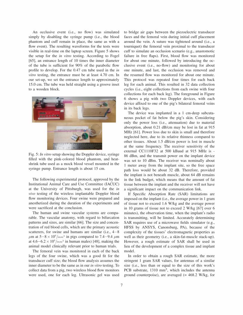
An occlusive event (i.e., no flow) was simulated
simply by disabling the syringe pump (i.e., the blood
phantom and cuff remain in place, the same as with a
flow event). The resulting waveforms for the tests were
visible in real-time on the laptop screen. Figure 5 shows
the setup for the in vitro testing. According to Fogel
[65], an entrance length of 10 times the inner diameter
of the tube is sufficient for 90% of the parabolic flow
profile to develop. For the 0.47 cm tube used in the invitro testing, the entrance must be at least 4.70 cm. In
our set-up, we set the entrance length to approximately
15.0 cm. The tube was held straight using a groove inset
to a wooden block.
Fig. 5: In vitro setup showing the Doppler device, syringe
filled with the pink-colored blood phantom, and heat-
shrink tube used as a mock blood vessel mounted in the
syringe pump. Entrance length is about 15 cm.
The following experimental protocol, approved by the
Institutional Animal Care and Use Committee (IACUC)
at the University of Pittsburgh, was used for the invivo testing of the wireless implantable Doppler blood
flow monitoring devices. Four swine were prepared and
anesthetized during the duration of the experiments and
were sacrificed at the conclusion.
The human and swine vascular systems are compa-
rable. The vascular anatomy, with regard to bifurcation
patterns and sizes, are similar [66]. The size and concen-
tration of red blood cells, which are the primary acoustic
scatterers, for swine and humans are similar (i.e., 4−8
μm at 5−8× 10⁶/mm3 in pigs compared to 7.4−9.4 μm
at 4.6−6.2× 10⁶/mm3 in human males) [48], making the
animal model clinically relevant prior to human trials.
The femoral vein was monitored in each of the back
legs of the four swine, which was a good fit for the
transducer cuff size; the blood flow analysis assumes the
inner diameter to be the same as in our in vitro testing. To
collect data from a pig, two wireless blood flow monitors
were used, one for each leg. Ultrasonic gel was used
to bridge air gaps between the piezoelectric transducer
faces and the femoral vein during initial cuff placement
around the vein. A suture was tightened around (i.e., a
tourniquet) the femoral vein proximal to the transducer
cuff to simulate an occlusion scenario (e.g., anastomotic
failure in free flaps). First, blood flow was monitored
for about one minute, followed by introducing the oc-
clusive event (i.e., no-flow) and monitoring for about
one minute, and last, the occlusion was removed and
the resumed flow was monitored for about one minute.
This protocol was repeated four times for each back
leg for each animal. This resulted in 32 data collection
cycles (i.e., eight collections from each swine with four
collections for each back leg). The foreground in Figure
6 shows a pig with two Doppler devices, with each
device affixed to one of the pig’s bilateral femoral veins
in its back legs.
The device was implanted in a 1 cm-deep subcuta-
neous pocket of fat below the pig’s skin. Considering
only the power loss (i.e., attenuation) due to material
absorption, about 0.21 dB/cm may be lost in fat at 915
MHz [61]. Power loss due to skin is small and therefore
neglected here, due to its relative thinness compared to
other tissues. About 1.5 dB/cm power is lost in muscle
at the same frequency. The receiver sensitivity of the
external CC1110F32 at 500 kBaud at 915 MHz is -
86 dBm, and the transmit power on the implant device
was set to 10 dBm. The receiver was nominally about
1 meter away from the implant site, so the free space
path loss would be about 32 dB. Therefore, provided
the implant is not beneath muscle, about 64 dB remains
in the link budget, which means that the amount of fat
tissue between the implant and the receiver will not have
a significant impact on the communication link.
If Specific Absorption Rate (SAR) limitations are
imposed on the implant (i.e., the average power in 1 gram
of tissue not to exceed 1.6 W/kg and the average power
in 10 grams of tissue not to exceed 2 W/kg [67] over 6
minutes), the observation time, when the implant’s radio
is transmitting, will be limited. Accurately determining
SAR requires use of a microwave fields simulator (e.g.,
HFSS by ANSYS, Canonsburg, PA), because of the
complexity of the tissues’ electromagnetic properties as
well as their geometry (i.e., a skin-fat-muscle stack-up).
However, a rough estimate of SAR shall be used in
lieu of the development of a complex tissue and implant
model.
In order to obtain a rough SAR estimate, the more
stringent 1 gram SAR values, for antennas of a similar
size (i.e., less than or equal to the size of this work’s
PCB substrate, 1310 mm3, which includes the antenna
ground counterpoise), are averaged (= 468.2 W/kg, for
7

1 W of delivered power to the antenna) from a 2012
literature review of implanted antennas for biomedical
telemetry by Kiourti and Nikita [68]. A radio packet is
transmitted every 7.74 ms; the packet transmission taking
5.02 ms, and the radio off-time is 2.72 ms (see Figure
4); all times were measured on a Saleae Logic 16 Logic
Analyzer (South San Francisco, CA). The CC1110F32 is
configured to deliver 10 mW to the implanted antenna;
however, taking into account the duty cycle (64.9%) of
wireless on-time due to packet transmission, the average
power continuously delivered to the antenna is 6.49 mW.
Using the maximum expected SAR of 468.2 W/kg from
literature, and the maximum permissible SAR of 1.6
W/kg over 6 minutes as per regulation, the maximum
allowable continuous power delivered to the antenna
cannot exceed 3.4 mW (= 1.6 W/kg468.2 W/kg ∗ 1 W ; calculated
according to Kim et al. [69]). Therefore, to meet this
requirement, the observation period using the developed
implant cannot exceed about 3 minutes and 9 seconds
(= 3.4 mW6.49 mW ∗ 6 minutes) for a single device during a 6
minute period. This estimate suggests that, for a single
implanted Doppler flow monitor, the data collection
protocol described earlier in this section complies with
safety regulations for power absorbed by the human
body.
Fig. 6: In vivo setup showing the Doppler devices
connected to the bilateral femoral veins in both back legs
of one pig. The encapsulated devices are shown exposed
solely for photographic illustration.
III. RESULTS
The developed device was slightly larger than a U.S.
Kennedy Half-dollar. The circular PCB substrate was
about 32.5 mm in diameter and 1.58 mm (i.e., thick
from top layer metal to bottom layer metal). The total
implanted electronics volume, including the antenna but
excluding the battery, was 1.70 cm3. The battery volume
was 4.4 cm3, and the total encapsulated volume (exclud-
ing the transducer apparatus and leads) was about 18.0
cm3.
A. In vitro performance
The in vitro testing served to characterize the per-
formance of the device. Real-time waveform data was
viewed on a laptop screen (Figure 8, reproduced in
MATLAB; also shown are time and voltage scales).
Here, the relative magnitudes of flow and no flow (i.e.,
simulating an occlusive event) conditions are shown.
Figure 7 shows the input-referred voltage noise of the
device, the differential voltage noise was measured at
the ADC inputs and divided by the midband receiver
chain voltage gain, 88 dB, referred to the LNA input.
The input-referred RMS voltage noise is 0.39 μV. Note
the visible common mode noise at 129 Hz, which is a
result of radio interference from the MCU’s radio, which
transmits a packet every 7.74 ms. The sensitivity, defined
as double the output-referred RMS noise voltage, of the
receiver chain is about -113 dBm (i.e., about 20 mVpeak
at the ADC) with the LNA matched to a 50Ω driver.
The input dynamic range is about 35 dB, and the output
voltage gain variation for an 400 Hz input tone (i.e.,
corresponding to about a 2.2 cm/s velocity) from -100
dBm to -78 dBm is 0.60 dB ±0.94 dB.
Fig. 7: Input-referred noise voltage at the LNA input
(i.e., output-referred noise divided by receiver chain
gain), and its RMS value, Vni,rms, is 0.39 μV. Common
mode noise is visible at 129 Hz, which is the period
between radio packet transmissions.
Figure 9a shows the effectiveness of using a moving
maximum filter to smooth the time-frequency spectro-
gram’s envelope of the Doppler signal. For this figure,
the expected flow was 34.15 mL/min (±1%) compared to
8

the procedure’s estimate of 34.2 mL/min, a relative error
between -0.8% and +1.2%. Figure 9b shows the perfor-
mance of the Doppler device across various expected
flow rates, as pumped by the NE-1000 syringe pump.
A moving minimum filter reduced measurement error
below 4.00 mL/min flow rates, while a moving maximum
filter reduced the error for rates above 3.00 mL/min. The
error bars encompass the relative error range due to the
±1% NE-1000 accuracy. The large relative errors for
low flow rates appears significant; however, the absolute
error in this flow rate range is small. For example, at 6.00
mL/min the relative error is the worst across the entirety
of measured data (i.e., between +12.1% and +9.8%), but
the absolute error is between +0.60 mL/min to +0.72
mL/min. Additionally, for 0.00 mL/min, the absolute
error is +0.40 mL/min; whereas, the relative error is
undefined. Above 6.00 mL/min, the measured flow rate
compared to the NE-1000 nameplate reference flow rate
is below below ±5.0%. Additionally, when considering
the error bars, for flow rates above 8.00 mL/min, the
relative error is within ±5.0% of the reference flow rate,
with the relative error tending towards about 0.0% as the
flow rate increases. A simple linear fit to the measured
data shows an absolute error that approaches about +0.24
mL/min at 0.00 mL/min and about -0.23 mL/min at the
largest extrapolated flow range, 100 mL/min. The key
results are that above a few mL/min in the measured
range, the system will overestimate the flow rate, and
for even low flow rates (i.e., above 6.00 mL/min), the
relative error is small, and as the flow rate increases, the
accuracy of the measurement increases as well.
Fig. 8: Oscilloscope-like view used on the laptop com-
puter for real-time blood flow assessment. The displayed
waveforms are the transduced baseband Doppler signals.
Window length is 244 data samples long (i.e., 14.9 ms).
(a)
(b)
Fig. 9: In vitro performance of the Doppler device using
a syringe pump to generate reference flow rates. (a)
Effectiveness of the moving maximum filter applied
to the envelope of the time-frequency spectrogram of
the Doppler signal. The reference flow rate was 34.15
mL/min, and the flow estimate was 34.2 mL/min. Note
C = 60 secmin ; (b) Performance evaluation of the Doppler
device comparing measured flow rate along with the
corresponding magnitude of the relative error. Note that
the relative error for 0.00 mL/min was omitted from the
figure because its value is undefined.
9
B. In vivo results
Figure 12 shows blood flow data collected from two
swine femoral veins. These results confirm the ability
of the implanted Doppler device to monitor blood flow
wirelessly, without the problematic tether to a bedside
monitoring device. The flow and no-flow portions of
the waveform in Figure 12 are displayed using the raw
ADC samples (i.e., without digital signal processing).
In the figure, distinctive regions of flow and no-flow are
clearly visible, and the restoration of flow (i.e., “release”
in the figure) after an occlusion shows the blood flow
waveform approaching nearly the same amplitude as the
pre-occlusion event.
In the figure, noise appears to be present during the
no-flow portion of the waveform. Potential sources of
noise can be a result of many culprits. Mixing spurs
generated in-band, local oscillator phase noise, tuned
circuits formed by the many bypass networks on the
PCB, the boost converter, or even insufficient decoupling
to prevent noise from being injected into the power
supply by broadband nonlinear circuitry, such as by the
mixer. Noise due to the surgeon mechanically manip-
ulating the tourniquet around the vessel is visible near
the boundary of “occlusion” and “release.” Biological
noise also contributes to the noisy baseline. Blood flow
in nearby adjacent vessels will be picked up by the trans-
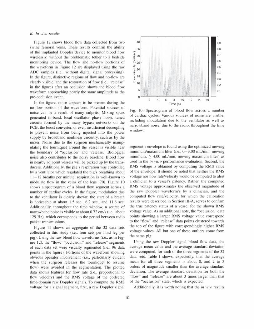
ducers. Additionally, the pig’s respiration was controlled
by a ventilator which regulated the pig’s breathing about
11−12 breaths per minute; respiration is well-known to
modulate flow in the veins of the legs [70]. Figure 10
shows a spectrogram of a blood flow segment across a
number of cardiac cycles. In the figure, modulation due
to the ventilator is clearly shown; the start of a breath
is noticeable at about 1.5 sec., 6.2 sec., and 11.6 sec.
Additionally, throughout the time window, a source of
narrowband noise is visible at about 0.72 cm/s (i.e., about
129 Hz), which corresponds to the period between radio
packet transmissions.
Figure 11 shows an aggregate of the 32 data sets
collected in this study (i.e., four sets per hind leg per
pig). Using the raw blood flow waveforms (i.e., as in Fig-
ure 12), the “flow,” “occlusion,” and “release” segments
of each data set were visually segmented (i.e., 96 data
points in the figure). Portions of the waveform showing
obvious operator involvement (i.e., particularly evident
when the surgeon releases the tourniquet to resume
flow) were avoided in the segmentation. The plotted
data shows features for flow rate (i.e., proportional to
flow velocity) and the RMS voltage of the collected
time-domain raw Doppler signals. To compute the RMS
voltage for a signal segment, first, a raw Doppler signal
Fig. 10: Spectrogram of blood flow across a number
of cardiac cycles. Various sources of noise are visible,
including modulation due to the ventilator as well as
narrowband noise, due to the radio, throughout the time
window.
segment’s envelope is found using the optimized moving
minimum/maximum filter (i.e., 0−3.00 mL/min: moving
minimum, ≥ 4.00 mL/min: moving maximum filter) as
used in the in vitro performance evaluation. Second, the
RMS voltage is obtained by computing the RMS value
of the envelope. It should be noted that neither the RMS
voltage nor flow rate/velocity would be computed to alert
a clinician to a vessel’s patency. Rather, the computed
RMS voltage approximates the observed magnitude of
the raw Doppler waveform’s by a clinician, and the
computed flow rate/velocity, for which the calibration
results were described in Section III-A, serves to confirm
the true patency status of a vessel for the shown RMS
voltage value. As an additional note, the “occlusion” data
points showing a larger RMS voltage value correspond
to the “flow” and “release” data points clustered towards
the top of the figure with correspondingly higher RMS
voltage values. All but one of these outliers come from
the same pig.
Using the raw Doppler signal blood flow data, the
average mean value and the average standard deviation
were computed, for each of the three segments of the 32
data sets. Table I shows, expectedly, that the average
mean for all three segments is about 0, and 2 to 3
orders of magnitude smaller than the average standard
deviation. The average standard deviation for both the
“flow” and “release” are about 3 times larger than that
of the “occlusion” state, which is expected.
Additionally, it is worth noting that the in vivo results
10

demonstrate the developed system’s ability to arbitrate
capturing blood flow from a specific device without
interference from nearby devices (i.e., as pictured in
Figure 6).
TABLE I: Average mean (μavg) and average standard
deviation (σavg) for all three flow segments. “*” denotes
multiplication with 10−4.
Flow Occlusion Releaseμavg (V) (−2.0± 10)∗ (−1.7± 10)∗ (−2.0± 11)∗σavg (V) 0.11± 0.14 0.030± 0.048 0.12± 0.18
Fig. 11: Aggregation of 32 data sets. Each data set
is segmented into three groups, “flow,” “occlusion,”
and “release.” The “occlusion” data points showing a
larger RMS voltage value correspond to the “flow” and
“release” data points clustered towards the top of the
figure with correspondingly higher RMS voltage values,
where all but one of these outliers come from the same
pig.
IV. DISCUSSION
The use of Doppler ultrasound to monitor blood flow
is a proven tool for general physiological monitoring.
Chronic implantation monitoring, postoperative monitor-
ing, and even freely behaving subject monitoring can
benefit from wireless blood flow systems. We demon-
strated a tool to simplify blood flow monitoring in veins
of the lower limbs, which are particularly difficult cases
for ultrasound operators [58], [59].
A simple real-time display was shown. Similar to the
wired gold standard in free flap monitoring, our system
reports vessel patency in a simple format. The in vitro
0 20 40 60 80 100 120 140 160 180−1
−0.8
−0.6
−0.4
−0.2
0
0.2
0.4
0.6
0.8
1
Time (s)
Nor
mal
ized
Am
plitu
de
Flow Occlusion Release
(a)
0 20 40 60 80 100 120 140 160 180−1
−0.8
−0.6
−0.4
−0.2
0
0.2
0.4
0.6
0.8
1
Time (s)
Nor
mal
ized
Am
plitu
de
Flow Occlusion Release
(b)
Fig. 12: (a) Collected Doppler signal from the femoral
vein in a swine’s left thigh using Device 1. (b) Collected
Doppler signal from the femoral vein in the same swine’s
right thigh using Device 2. Flow and no-flow/occlusion
conditions are shown in the figures using the experimen-
tal data collection protocol from Section II-C.
performance evaluation showed close agreement with the
reference flow rates. Above 8.00 mL/min, its relative
error is within ±5.0% for the measured data (i.e., in-
cluding the instrument uncertainty of the NE-1000), and
fitting to the measured data uncovers maximum absolute
errors of +0.24 mL/min for a 0.00 mL/min reference
and about -0.23 mL/min at the largest extrapolated flow
range, 100 mL/min. Other reported continuous wave
wireless totally implantable Doppler devices in literature
describe their accuracy in various ways. Using a steady
state flow simulator, Meindl and Di Pietro report a ±20%
11

center velocity accuracy compared to theory, across any
vessel size with any flow profile [64]. Yonezawa et al.
reported ±1% linearity to the reference flow value, via
a timed volume collection method, between 20 cm/s
− 150 cm/s flow velocities [51]. Vilkomerson et al.
reported velocity accuracy errors less than 5% over a 100
mL/min to 900 mL/min range using a volume collection
method [56], [71]. Using custom-built flow phantom,
comprising a gear pump to hydraulically compress a pair
of bellows filled with a blood-mimicking fluid [72] in
an alternating fashion followed by a volume collection
method, Cannata et al. reported average flow velocity
estimate errors less than 6% for 30 measurements over
a 2.5-hour period across a 60 mL/min to 500 mL/min
flow rate range [57]. Additionally, Cannata et al reported
a 1.7% lower peak flow velocity compared with a duplex
ultrasound system when measuring a rabbit’s infrarenal
aorta. Tang et al. described a system with about 5.83%
deviation from the expected flow velocity, 24 cm/s, using
a timed volume method, but only for a single reported
measurement [54]. Considering the various descriptions
and conditions of reported device accuracy, the calibrated
accuracy of our presented system appears to report
a better accuracy over its calibrated range (i.e., 0.00
mL/min to 34.15 mL/min; 0.00 cm/s to 3.2 cm/s) than
found elsewhere in literature (i.e., note that the relative
error, described in our calibrated results, is misleading
for very low flow rates). It should be noted that the
accuracy of the described system relies not only on
the implanted wireless Doppler device, but the flow
estimation methodology (i.e., averaging filters used in
the time-frequency domain) described in Section II-C.
The in vivo results show that, while the majority of
“occlusion” segments were clustered near 0 mL/ms with
near 0 VRMS amplitude, there was a minority grouping
that showed non-zero RMS voltages for near-zero flow
rates. This minority grouping also shows concomitant
larger “flow” and “release” RMS values compared to
those of the rest of the data in Figure 11 (i.e., clustered
near the top of the figure). The reason for the discrepancy
is that flow/velocity estimation begins with a moving
minimum filter, and only uses a moving maximum filter
if the flow rate is greater than 3.00 mL/min; whereas, the
RMS voltage estimation always uses a moving maximum
filter, leading to non-zero RMS voltages for near-zero
flow rates. Mechanical perturbations of the pig’s body
due to a ventilator, which is used to control the pig’s
respiration, manifest as periodic modulation of the raw
Doppler waveform (See Figure 10). This periodic noise
results in larger accumulated overestimation of the en-
velope when using a moving maximum filter. Therefore,
data in which the periodic noise due to the ventilator
is more pronounced will result in, for the “occlusion”
case, as an example, larger non-zero RMS voltages while
the flow rate/velocity remaining still near-zero. As a
consequence, the implication is that, when using this
developed Doppler system, establishing a baseline RMS
voltage reading is necessary so that future assessments
of anastomotic patency are valid. For example, if no
baseline RMS value (i.e., baseline flow and baseline no-
flow magnitudes) was established for the “occlusion”
value near 0.37 V RMS, it is likely that a clinician would
report a false-positive for blood flow (i.e., the flow rate
for this data point is actually near 0 mL/min while the
raw Doppler signal magnitude is larger than that for
“flow” or “release” of other pigs) if only the absolute
magnitude of the signal were considered. Nonetheless,
it should be noted that in the majority data group, the
absolute magnitude of the “occlusion” RMS voltage
value predictably falls below the “flow” and “release”
RMS voltage values.
Several outliers in the in vivo results (Figure 11)
show a non-zero RMS voltage for a near-zero “flow”
and “release” flow velocity/rate: one “flow”/“release”
pair and another lone “release” component. Both can
be explained by poor transducer coupling, likely due
to operator involvement, resulting in a low signal-to-
noise ratio and leading to a poor flow/velocity estimation.
The ventilator noise resulted in the non-zero RMS volt-
age. The calibration procedure was void of noise and
perturbations. So while the calibrated data show close
agreement with theory, it is not known the degree to
which noise and perturbations, such as those introduced
by the pig’s ventilator, affect the estimate of flow rate.
To the best of the authors’ knowledge, considering
the electronics and antenna size, we have demonstrated
the smallest wireless implantable blood flow monitor
device that incorporates an MCU. The PCB area is about
8.30 cm2 (i.e., single side). The electronics, including
the antenna and without battery, is about 1.70 cm3,
and the total encapsulated volume, without transducer
cuff and transducer leads, is about 18.0 cm3. Because
the implant lifetime was short, encapsulation was not
optimized, which added significant bulk (i.e., 6.08 cm3
without encapsulation; includes electronics and battery).
Total implant volume can be reduced through the use
of alternative encapsulation materials (e.g., silicones,
epoxies, glass, etc. [73], [74]). Kiourti and Nikita provide
suggestions for biocompatible encapsulation options for
implantable antennas in order to minimize power loss
[68]. The wireless blood flow monitor PCBs developed
by Vilkomerson et al. appears to occupy about 30.5 cm2
(i.e., total, for both PCBs, single side) from published
images [56]. The implant volume is not given. Cannata’s
12

work stated that it used a modified version of Vilkomer-
son’s design, without commenting on the specific size
[57]. Another device, developed by Tang, Vilkomerson,
and Chilipka, demonstrated an implantable blood flow
monitor with a wireless rechargeable battery; the battery
was recharged by a coil [54]. The reported total PCB area
(i.e., for two boards) was 7 cm2, but implant volume (i.e.,
with batteries, without batteries, without encapsulation,
etc.) was not reported. Additionally, the implant volume
impact by the coil was not reported. Additionally, one re-
ported device in literature, called an anastomotic patency
monitor, which used a microcontroller, reported good
agreement between its measured flow and actual flow
[75]; however, size and design specifics were omitted.
Previous microcontroller-equipped wireless blood
flow monitors have not focused significant attention on
the impact of circuit selection, performance, degree of
integration, and topology to reduce PCB real-estate and
implant size. Our device was able to achieve its size
through the following considerations. High density PCBs
which mount components on both sides and in close
proximity reduce size, but interference is a significant
concern, so care was taken to avoid a troublesome lay-
out while minimizing real-estate. Differential electronics
were used wherever possible to minimize the effects
of coupled noise, thereby allowing for a more compact
layout. Power supply decoupling was incorporated, and
dedicated voltage regulators for most portions of the
design were used to prevent noisy circuits from polluting
power supply lines. The MCU, which incorporated both
a microcontroller and a radio, saved significant real-
estate by offering a high degree of functionality in
a single package. The radio telemetry frequency was
selected such that the antenna’s size would not incur
a significant real-estate penalty. However, the caveat is
that while higher frequencies typically permit smaller
antenna geometries [76], the losses in biological tissues
at higher frequencies are often greater [77].
The same MCU that allows software customization
to control system functions [78], blood flow data cap-
turing, and low power modes, can also be used to
develop a scalable system [79], which can interrogate
and control multiple devices. Examples where multiple
monitors need to be used in close proximity include,
free flaps requiring in-flow and out-flow monitoring, and
hospitals with nearby patients being monitored. Thus far,
there has been no report in literature of wireless blood
flow monitoring systems supporting multiple monitors.
With our developed system, a specific monitor could be
activated, wirelessly, without activating unwanted nearby
monitors.
The MCU software can be readily customized for
specific applications. For example, the software could be
customized to set the sleep timer duration dynamically,
thereby extending implant lifetime and enabling chronic
implantation applications [80]. As another example, the
abort key could be modified in our current implemen-
tation. Currently, all devices respond to the same abort
sequence, as a failsafe to prevent accidentally leaving
a device activated and draining its battery. For a large
scale deployable system, this should be changed to only
abort a specific device. The current system uses 16-bit
abort keys and “Wake Up” SIDs. This means that 216/2unique devices can be multiplexed (i.e., one unique abort
key and one unique “Wake Up” SID per device).
V. CONCLUSION
This paper demonstrates a wireless Doppler blood
flow monitoring system that reduces flow interpretation
difficulties by providing a simple real-time visual in-
dicator of blood flow. The developed system’s blood
flow rate accuracy is high across its calibrated range.
Careful selection of circuit performance, degree of in-
tegration, and topology resulted in a compact implant
size. The microcontroller unit played a crucial role in
size reduction. Additionally, it allowed implementing
customized software, which extended battery life and
permitted the activation of specific blood flow monitors
in the presence of nearby monitors. In the future, the
customizable software can be adapted to deploy a large
scale monitoring system with thousands of monitors
accessible from just a single external hub. And most
importantly, system functions that heavily impact battery
life can be dynamically set via the microcontroller unit
in order to satisfy chronic implantation applications.
ACKNOWLEDGMENTS
The study was supported by the Heinz Endowments
under award number C1742.
REFERENCES
[1] M. J. Kang, C. H. Chung, Y. J. Chang, and K. H. Kim,“Reconstruction of the lower extremity using free flaps,” Archivesof Plastic Surgery, vol. 40, no. 5, pp. 575–583, 2013.
[2] A. J. Organek, M. J. Klebuc, and R. M. Zuker, “Indications andoutcomes of free tissue transfer to the lower extremity in children:review,” Journal of Reconstructive Microsurgery, vol. 22, no. 3,pp. 173–182, 2006.
[3] W. Zhou, M. He, Y. Liao, and Z. Yao, “Reconstructing a complexcentral facial defect with a multiple-folding radial forearm flap,”Journal of Oral and Maxillofacial Surgery: Official Journal ofthe American Association of Oral and Maxillofacial Surgeons,vol. 72, no. 4, pp. 836.e1–4, 2014.
[4] R. Yanko-Arzi, E. Gur, A. Margulis, J. Bickels, S. Dadia,Y. Gortzak, and A. Zaretski, “The role of free tissue transferin posterior neck reconstruction,” Journal of Reconstructive Mi-crosurgery, vol. 30, no. 5, pp. 305–312, 2014.
13

[5] G. D. Rosson, M. Magarakis, S. M. Shridharani, S. M. Stapleton,L. K. Jacobs, M. A. Manahan, and J. I. Flores, “A review of thesurgical management of breast cancer: plastic reconstructive tech-niques and timing implications,” Annals of Surgical Oncology,vol. 17, no. 7, pp. 1890–1900, 2010.
[6] M. L. Urken, H. Weinberg, D. Buchbinder, J. F. Moscoso,W. Lawson, P. J. Catalano, and H. F. Biller, “Microvascular freeflaps in head and neck reconstruction: report of 200 cases andreview of complications,” Archives of Otolaryngology–Head andNeck Surgery, vol. 120, no. 6, pp. 633–640, 1994.
[7] V. K. Tiwari, S. Sarabahi, and S. Chauhan, “Preputial flap as anadjunct to groin flap for the coverage of electrical burns in thehand,” Burns, vol. 40, no. 1, pp. 4–7, 2014.
[8] C. Firat and Y. Geyik, “Surgical modalities in gunshot woundsof the face,” Journal of Craniofacial Surgery, vol. 24, no. 4, pp.1322–1326, 2013.
[9] I. D. Papel, Facial plastic and reconstructive surgery, 3rd ed.New York: Thieme, 2009.
[10] G. I. Taylor and R. K. Daniel, “The anatomy of several free flapdonor sites,” Plastic and Reconstructive Surgery, vol. 56, no. 3,pp. 243–253, 1975.
[11] C. E. Attinger, I. Ducic, C. L. Hess, A. Basil, M. Abbruzzesse,and P. Cooper, “Outcome of skin graft versus flap surgery inthe salvage of the exposed Achilles tendon in diabetics versusnondiabetics,” Plastic and Reconstructive Surgery, vol. 117,no. 7, pp. 2460–2467, 2006.
[12] M. Godina, “Preferential use of end-to-side arterial anastomosesin free flap transfers,” Plastic and Reconstructive Surgery, vol. 64,no. 5, pp. 673–682, 1979.
[13] B. O’Brien, W. A. Morrison, H. Ishida, A. M. MacLeod, andA. Gilbert, “Free flap transfers with microvascular anastomoses,”British Journal of Plastic Surgery, vol. 27, no. 3, pp. 220–230,1974.
[14] W. A. Goodstein and H. J. Buncke Jr, “Patterns of vascularanastomoses vs. success of free groin flap transfers,” Plastic andReconstructive Surgery, vol. 64, no. 1, pp. 37–40, 1979.
[15] B. Strauch and H.-L. Yu, Atlas of microvascular surgery:anatomy and operative techniques. Thieme, 2006.
[16] W. M. Swartz, J. C. Banis, and G. M. Buncke, “Head and neckmicrosurgery,” Annals of Plastic Surgery, vol. 29, no. 4, p. 381,1992.
[17] K. Z. Paydar, S. L. Hansen, D. S. Chang, W. Y. Hoffman, andP. Leon, “Implantable venous Doppler monitoring in head andneck free flap reconstruction increases the salvage rate,” Plasticand Reconstructive Surgery, vol. 125, no. 4, pp. 1129–1134,2010.
[18] C.-C. Wu, P.-Y. Lin, K.-Y. Chew, and Y.-R. Kuo, “Free tissuetransfers in head and neck reconstruction: complications, out-comes and strategies for management of flap failure: analysis of2019 flaps in single institute,” Microsurgery, vol. 34, no. 5, pp.339–344, 2014.
[19] K.-T. Chen, S. Mardini, D. C.-C. Chuang, C.-H. Lin, M.-H.Cheng, Y.-T. Lin, W.-C. Huang, C.-K. Tsao, and F.-C. Wei,“Timing of presentation of the first signs of vascular compromisedictates the salvage outcome of free flap transfers,” Plastic andReconstructive Surgery, vol. 120, no. 1, pp. 187–195, 2007.
[20] D. Novakovic, R. S. Patel, D. P. Goldstein, and P. J. Gullane,“Salvage of failed free flaps used in head and neck reconstruc-tion,” Head and Neck Oncology, vol. 1, no. 1, pp. 1–5, 2009.
[21] J. P. Fischer, J. A. Nelson, B. Sieber, E. Cleveland, S. J.Kovach, L. C. Wu, J. M. Serletti, and S. Kanchwala, “Freetissue transfer in the obese patient: an outcome and cost analysisin 1258 consecutive abdominally based reconstructions,” Plasticand Reconstructive Surgery, vol. 131, no. 5, pp. 681–692, 2013.
[22] X. F. Ling and X. Peng, “What is the price to pay for a free fibulaflap? a systematic review of donor-site morbidity following freefibula flap surgery,” Plastic and Reconstructive Surgery, vol. 129,no. 3, pp. 657–674, 2012.
[23] A. O. Momoh, P. Yu, R. J. Skoracki, S. Liu, L. Feng, andM. M. Hanasono, “A prospective cohort study of fibula free flapdonor-site morbidity in 157 consecutive patients,” Plastic andRconstructive Surgery, vol. 128, no. 3, pp. 714–720, 2011.
[24] K. C. Shestak and N. F. Jones, “Microsurgical free-tissue trans-fer in the elderly patient,” Plastic and Reconstructive Surgery,vol. 88, no. 2, pp. 259–263, 1991.
[25] R. E. H. Ferguson Jr and P. Yu, “Techniques of monitoring buriedfasciocutaneous free flaps,” Plastic and Reconstructive Surgery,vol. 123, no. 2, pp. 525–532, 2009.
[26] J. M. Smit, I. S. Whitaker, A. G. Liss, T. Audolfsson, M. Kil-dal, and R. Acosta, “Post operative monitoring of microvas-cular breast reconstructions using the implantable Cook-SwartzDoppler system: A study of 145 probes & technical discussion,”Journal of Plastic, Reconstructive and Aesthetic Surgery, vol. 62,no. 10, pp. 1286–1292, 2009.
[27] B. C. Cho, D. P. Shin, J. S. Byun, J. W. Park, and B. S. Baik,“Monitoring flap for buried free tissue transfer: its importanceand reliability,” Plastic and Reconstructive Surgery, vol. 110,no. 5, pp. 1249–1258, 2002.
[28] J. P. Fischer, B. Sieber, J. A. Nelson, E. Cleveland, S. J. Kovach,L. C. Wu, S. Kanchwala, and J. M. Serletti, “Comprehensiveoutcome and cost analysis of free tissue transfer for breastreconstruction: an experience with 1303 flaps,” Plastic andReconstructive Surgery, vol. 131, no. 2, pp. 195–203, 2013.
[29] G. M. Kind, R. F. Buntic, G. M. Buncke, T. M. Cooper, P. P. Siko,and H. J. Buncke Jr, “The effect of an implantable Doppler probeon the salvage of microvascular tissue transplants,” Plastic andReconstructive Surgery, vol. 101, no. 5, pp. 1268–1273, 1998.
[30] W. M. Swartz, R. Izquierdo, and M. J. Miller, “Implantable ve-nous Doppler microvascular monitoring: Laboratory investigationand clinical results,” Plastic and Reconstructive Surgery, vol. 93,no. 1, pp. 152–163, 1994.
[31] C. Holm, J. Tegeler, M. Mayr, A. Becker, U. Pfeiffer, andW. Muhlbauer, “Monitoring free flaps using laser-induced flu-orescence of indocyanine green: A preliminary experience,”Microsurgery, vol. 22, no. 7, pp. 278–287, 2002.
[32] M. S. Irwin, M. S. Thorniley, C. J. Dore, and C. J. Green,“Near infra-red spectroscopy: a non-invasive monitor of perfusionand oxygenation within the microcirculation of limbs and flaps,”British Journal of Plastic Surgery, vol. 48, no. 1, pp. 14–22,1995.
[33] A. Keller, “Noninvasive tissue oximetry for flap monitoring: aninitial study,” Journal of Reconstructive Microsurgery, vol. 23,no. 4, pp. 189–198, 2007.
[34] R. K. Khouri and W. W. Shaw, “Monitoring of free flapswith surface-temperature recordings: is it reliable?” Plastic andReconstructive Surgery, vol. 89, no. 3, pp. 495–499, 1992.
[35] C. A. Stone, P. A. Dubbins, and R. J. Morris, “Use of colourduplex Doppler imaging in the postoperative assessment of buriedfree flaps,” Microsurgery, vol. 21, no. 5, pp. 223–227, 2001.
[36] J. K. Choi, M. G. Choi, J. M. Kim, and H. M. Bae, “Efficient dataextraction method for near-infrared spectroscopy (NIRS) systemswith high spatial and temporal resolution,” IEEE Transactionson Biomedical Circuits and Systems, vol. 7, no. 2, pp. 169–177,2013.
[37] M. Sawan, M. T. Salam, J. Le Lan, A. Kassab, S. Gelinas, P. Van-nasing, F. Lesage, M. Lassonde, and D. K. Nguyen, “Wirelessrecording systems: From noninvasive EEG-NIRS to invasive EEGdevices,” IEEE Transactions on Biomedical Circuits and Systems,vol. 7, no. 2, pp. 186–195, 2013.
[38] W. M. Swartz, N. F. Jones, L. Cherup, and A. Klein, “Direct mon-itoring of microvascular anastomoses with the 20-MHz ultrasonicDoppler probe: An experimental and clinical study,” Plastic andReconstructive Surgery, vol. 81, no. 2, pp. 149–158, 1988.
[39] B. Fernando, V. L. Young, and S. E. Logan, “Miniature im-plantable laser Doppler probe monitoring of free tissue transfer,”Annals of Plastic Surgery, vol. 20, no. 5, pp. 434–442, 1988.
14

[40] P. M. Parker, J. C. Fischer, and W. W. Shaw, “Implantablepulsed Doppler cuff for long-term monitoring of free flaps: Apreliminary study,” Microsurgery, vol. 5, no. 3, pp. 130–135,1984.
[41] J. M. Smit, C. J. Zeebregts, R. Acosta, and P. M. N. Werker,“Advancements in free flap monitoring in the last decade: acritical review,” Plastic and Reconstructive Surgery, vol. 125,no. 1, pp. 177–185, 2010.
[42] J. P. Guillemaud, H. Seikaly, D. Cote, H. Allen, and J. R. Harris,“The implantable Cook-Swartz Doppler probe for postoperativemonitoring in head and neck free flap reconstruction,” Archivesof Otolaryngology–Head and Neck Surgery, vol. 134, no. 7, pp.729–734, 2008.
[43] S. G. Pryor, E. J. Moore, and J. L. Kasperbauer, “ImplantableDoppler flow system: Experience with 24 microvascular free-flap operations,” Otolaryngology-Head and Neck Surgery, vol.135, no. 5, pp. 714–718, 2006.
[44] D. W. Oliver, I. S. Whitaker, H. Giele, P. Critchley, and O. Cas-sell, “The Cook-Swartz venous Doppler probe for the post-operative monitoring of free tissue transfers in the United King-dom: a preliminary report,” British Journal of Plastic Surgery,vol. 58, no. 3, pp. 366–370, 2005.
[45] W. M. Rozen, G. G. Ang, A. H. McDonald, G. Sivarajah,R. Rahdon, R. Acosta, and D. J. Thomas, “Sutured attachment ofthe implantable Doppler probe cuff for large or complex pediclesin free tissue transfer,” Journal of Reconstructive Microsurgery,vol. 27, no. 2, pp. 99–102, 2011.
[46] T. R. Nelson and D. H. Pretorius, “The Doppler signal: wheredoes it come from and what does it mean?” American Journalof Roentgenology, vol. 151, no. 3, pp. 439–447, 1988.
[47] Y. F. Law, P. A. Bascom, K. W. Johnston, P. Vaitkus, and R. S.Cobbold, “Experimental study of the effects of pulsed Dopplersample volume size and position on the Doppler spectrum,”Ultrasonics, vol. 29, no. 5, pp. 404–410, 1991.
[48] K. K. Shung and G. A. Thieme, Ultrasonic scattering in biolog-ical tissues. CRC Press, 1992.
[49] J. J. Rosenberg, B. D. Fornage, and P. M. Chevray, “Monitoringburied free flaps: limitations of the implantable Doppler and useof color duplex sonography as a confirmatory test,” Plastic andReconstructive Surgery, vol. 118, no. 1, pp. 109–113, 2006.
[50] D. E. Franklin, N. W. Watson, K. E. Pierson, and R. L.Van Citters, “Technique for radio telemetry of blood-flow velocityfrom unrestrained animals,” The American Journal of MedicalElectronics, vol. 5, no. 1, pp. 24–28, 1965.
[51] Y. Yonezawa, T. Nakayama, I. Ninomiya, and W. M. Caldwell,“Radio telemetry directional ultrasonic blood flowmeter for usewith unrestrained animals,” Medical and Biological Engineeringand Computing, vol. 30, no. 6, pp. 659–665, 1992.
[52] R. Gill and J. D. Meindl, “Low power integrated circuits for animplantable pulsed Doppler ultrasonic blood flowmeter,” IEEEJournal of Solid-State Circuits, vol. 10, no. 6, pp. 464–471, 1975.
[53] D. M. DiPietro and J. D. Meindl, “Integrated circuits for animplantable CW Doppler ultrasonic flowmeter,” IEEE Journalof Solid-State Circuits, vol. 12, no. 5, pp. 573–576, 1977.
[54] S. C. Tang, D. Vilkomerson, and T. Chilipka, “Magnetically-powered implantable Doppler blood flow meter,” in 2014 IEEEInternational Ultrasonics Symposium. IEEE, 2014, pp. 1622–1625.
[55] E. Sejdic, M. A. Rothfuss, M. L. Gimbel, and M. H. Mickle,“Comparative analysis of compressive sensing approaches forrecovery of missing samples in implantable wireless dopplerdevice,” IET Signal Processing, vol. 8, no. 3, pp. 230–238, 2014.
[56] D. Vilkomerson, T. Chilipka, J. Bogan, J. Blebea, R. Choudry,J. Wang, M. Salvatore, V. Rotella, and K. Soundararajan, “Im-plantable ultrasound devices,” in Proc. SPIE 6920, MedicalImaging 2008: Ultrasonic Imaging and Signal Processing, vol.6920. International Society for Optics and Photonics, March2008, pp. 69 200C–69 200C–11.
[57] J. M. Cannata, T. Chilipka, H.-C. Yang, S. Han, S. W. Ham,V. L. Rowe, F. A. Weaver, K. K. Shung, and D. Vilkomerson,“Development of a flexible implantable sensor for postoperativemonitoring of blood flow,” Journal of Ultrasound in Medicine,vol. 31, no. 11, pp. 1795–1802, 2012.
[58] A. I. Galeandro, G. Quistelli, P. Scicchitano, M. Gesualdo,A. Zito, P. Caputo, R. Carbonara, G. Galgano, F. Ciciarello,S. Mandolesi, C. Franceschi, and M. M. Ciccone, “Dopplerultrasound venous mapping of the lower limbs,” Vascular Healthand Risk Management, vol. 8, p. 59, 2012.
[59] J. M. Porter, G. L. Moneta, and An International ConsensusCommittee on Chronic Venous Disease, “Reporting standards invenous disease: an update,” Journal of Vascular Surgery, vol. 21,no. 4, pp. 635–645, 1995.
[60] E. J. Boote, “AAPM/RSNA physics tutorial for residents: Topicsin US: Doppler US techniques: Concepts of blood flow detectionand flow dynamics 1,” Radiographics, vol. 23, no. 5, pp. 1315–1327, 2003.
[61] H. Park, M. Kiani, H. M. Lee, J. Kim, J. Block, B. Gosselin,and M. Ghovanloo, “A wireless magnetoresistive sensing systemfor an intraoral tongue-computer interface,” IEEE Transactionson Biomedical Circuits and Systems, vol. 6, no. 6, pp. 571–585,2012.
[62] R. W. Gill, “Measurement of blood flow by ultrasound: accuracyand sources of error,” Ultrasound in Medicine and Biology,vol. 11, no. 4, pp. 625–641, 1985.
[63] M. Thiriet, Biology and Mechanics of Blood Flows: Part II:Mechanics and Medical Aspects. Springer Science & BusinessMedia, 2007, vol. 2.
[64] D. M. Di Pietro and J. D. Meindl, “Optimal system designfor an implantable CW Doppler ultrasonic flowmeter,” IEEETransactions on Biomedical Engineering, no. 3, pp. 255–264,1978.
[65] M. A. Fogel, Ventricular function and blood flow in congenitalheart disease. John Wiley & Sons, 2008.
[66] W. Luo, H. Hosseini, V. Zderic, F. Mann, G. O’Keefe, andS. Vaezy, “Detection and localization of peripheral vascularbleeding using doppler ultrasound,” The Journal of emergencymedicine, vol. 41, no. 1, pp. 64–73, 2011.
[67] A. Kiourti, M. Christopoulou, and K. S. Nikita, “Performanceof a novel miniature antenna implanted in the human head forwireless biotelemetry,” in 2011 IEEE International Symposiumon Antennas and Propagation. IEEE, 2011, pp. 392–395.
[68] A. Kiourti and K. S. Nikita, “A review of implantable patchantennas for biomedical telemetry: Challenges and solutions[wireless corner],” IEEE Antennas and Propagation Magazine,vol. 54, no. 3, pp. 210–228, 2012.
[69] J. Kim and Y. Rahmat-Samii, “Implanted antennas inside ahuman body: Simulations, designs, and characterizations,” IEEETransactions on Microwave Theory and Techniques, vol. 52,no. 8, pp. 1934–1943, 2004.
[70] W. E. Brant, The Core Curriculum, Ultrasound. LippincottWilliams & Wilkins Philadelphia, 2001.
[71] D. Vilkomerson and T. Chilipka, “Implantable Doppler systemfor self-monitoring vascular grafts,” in Ultrasonics Symposium,2004 IEEE, vol. 1, Aug 2004, pp. 461–465 Vol.1.
[72] K. V. Ramnarine, D. K. Nassiri, P. R. Hoskins, and J. Lubbers,“Validation of a new blood-mimicking fluid for use in Dopplerflow test objects,” Ultrasound in medicine & biology, vol. 24,no. 3, pp. 451–459, 1998.
[73] D. Zhou and E. Greenbaum, Implantable Neural Prostheses 2:Techniques and Engineering Approaches, ser. Biological andMedical Physics, Biomedical Engineering. Springer, 2010.
[74] S. Park, D. A. Borton, M. Kang, A. V. Nurmikko, and Y.-K.Song, “An implantable neural sensing microsystem with fiber-optic data transmission and power delivery,” Sensors, vol. 13,no. 5, pp. 6014–6031, 2013.
[75] P. F. K. Read, R. W. Martin, E. H. Albrecht, and A. H. Proctor,“Implantable Doppler ultrasonic vessel patency monitor,” in
15

Proceedings of the Annual International Conference of the IEEEEngineering in Medicine and Biology Society. IEEE, 1989, pp.1106–1107.
[76] C. A. Balanis, Antenna theory: analysis and design. New YorkCity, NY: Wiley, 2012.
[77] S. Gabriel, R. W. Lau, and C. Gabriel, “The dielectric propertiesof biological tissues: II. measurements in the frequency range 10Hz to 20 GHz,” Physics in Medicine and Biology, vol. 41, no. 11,p. 2251, 1996.
[78] X. Chen, X. Zhang, L. Zhang, X. Li, N. Qi, H. Jiang, andZ. Wang, “A wireless capsule endoscope system with low-power controlling and processing ASIC,” IEEE Transactions onBiomedical Circuits and Systems, vol. 3, no. 1, pp. 11–22, 2009.
[79] R. S. Dilmaghani, H. Bobarshad, M. Ghavami, S. Choobkar, andC. Wolfe, “Wireless sensor networks for monitoring physiologicalsignals of multiple patients,” IEEE Transactions on BiomedicalCircuits and Systems, vol. 5, no. 4, pp. 347–356, 2011.
[80] X. Zhang, H. Jiang, L. Zhang, C. Zhang, Z. Wang, and X. Chen,“An energy-efficient ASIC for wireless body sensor networks inmedical applications,” IEEE Transactions on Biomedical Circuitsand Systems, vol. 4, no. 1, pp. 11–18, 2010.
16