Vietnam J Comput Sci (2014) 1:79–95DOI 10.1007/s40595-013-0008-z

REGULAR PAPER

A survey on software fault detection based on different predictionapproaches

Golnoush Abaei · Ali Selamat

Received: 23 October 2013 / Accepted: 23 October 2013 / Published online: 30 November 2013© The Author(s) 2013. This article is published with open access at Springerlink.com

Abstract One of the software engineering interests is qual-ity assurance activities such as testing, verification and vali-dation, fault tolerance and fault prediction. When any com-pany does not have sufficient budget and time for testing theentire application, a project manager can use some fault pre-diction algorithms to identify the parts of the system that aremore defect prone. There are so many prediction approachesin the field of software engineering such as test effort, secu-rity and cost prediction. Since most of them do not have astable model, software fault prediction has been studied inthis paper based on different machine learning techniquessuch as decision trees, decision tables, random forest, neuralnetwork, Naïve Bayes and distinctive classifiers of artificialimmune systems (AISs) such as artificial immune recogni-tion system, CLONALG and Immunos. We use four publicNASA datasets to perform our experiment. These datasets aredifferent in size and number of defective data. Distinct para-meters such as method-level metrics and two feature selectionapproaches which are principal component analysis and cor-relation based feature selection are used to evaluate the finestperformance among the others. According to this study, ran-dom forest provides the best prediction performance for largedata sets and Naïve Bayes is a trustable algorithm for smalldata sets even when one of the feature selection techniquesis applied. Immunos99 performs well among AIS classifierswhen feature selection technique is applied, and AIRSParal-lel performs better without any feature selection techniques.The performance evaluation has been done based on threedifferent metrics such as area under receiver operating char-

G. Abaei · A. Selamat (B)Faculty of Computing, University Technology Malaysia,Johor Baharu, 81310 Johor, Malaysiae-mail: aselamat@utm.my

G. Abaeie-mail: golnoosh.abaee@gmail.com

acteristic curve, probability of detection and probability offalse alarm. These three evaluation metrics could give thereliable prediction criteria together.

Keywords Software fault prediction · Artificial immunesystem · Machine learning · AISParallel · CSCA · Randomforest

1 Introduction

As today’s software grows rapidly in size and complexity,the prediction of software reliability plays a crucial role insoftware development process [1]. Software fault is an errorsituation of the software system that is caused by explicit andpotential violation of security policies at runtime because ofwrong specification and inappropriate development of con-figuration [2]. According to [3], analyzing and predictingdefects1 are needed for three main purposes, firstly, forassessing project progress and plan defect detection activ-ities for the project manager. Secondly, for evaluating prod-uct quality and finally for improving capability and assess-ing process performance for process management. In faultprediction, previous reported faulty data with the help ofdistinct metrics identify the fault-prone modules. Importantinformation about location, number of faults and distributionof defects are extracted to improve test efficiency and soft-ware quality of the next version of the software. Two bene-fits of software fault prediction are improvement of the testprocess by focusing on fault-prone modules and by identifi-cation the refactoring candidates that are predicted as fault-prone [4]. Numbers of different methods were used for soft-ware fault prediction such as genetic programming, decision

1 Defects and faults have the same meaning in this paper.

123

80 Vietnam J Comput Sci (2014) 1:79–95

trees, neural network, distinctive Naïve Bayes approaches,fuzzy logic and artificial immune system (AIS) algorithms.Almost all software fault prediction studies use metrics andfaulty data of previous software release to build fault predic-tion models, which is called supervised learning approaches.Supervised machine learning classifiers consist of two phases:training and test phase; the result of training phase is a modelthat is applied to the testing data to do some prediction [5].There are some other methods like clustering, which could beused when there are no previous available data; these methodsare known as unsupervised learning approaches. It should bementioned that some researchers like Koksal et al. [6] usedanother classification for data mining methods, which arefamous as descriptive and predicative.

One of the main challenges in this area is how to get thedata. In some works like in [7], a specific company pro-vides the data, so the results are not fully trustable. Before2005, more than half of the researches have used non-publicdatasets; however after that, with the help of PROMISErepository, the usage of public datasets reached to half [8],because the results are more reliable and not specific to aparticular company. According to [8], software fault predic-tions are categorized based on several criteria such as metrics,datasets and methods. According to the literatures, softwarefault prediction models are built based on different set of met-rics; method-level and class-level are two of the most impor-tant ones. Method-level metrics are suitable for both proce-dural and object-oriented programming style whereas class-level metrics are extracted based on object-oriented notation.It should be mentioned that compared to the other metrics,the method-level metrics is still the most dominant metricsprediction, followed by class-level metrics in fault predic-tion research area and machine-learning algorithms. It has

been for many years that researchers work on different typesof algorithms based on machine learning, statistical meth-ods and sometimes the combination of them. In this paper,the experiments have been done on four NASA datasets withdifferent population size using two distinct feature selectiontechniques that are principal component analysis (PCA) andcorrelation-based feature selection (CFS). We have changedthe defect rates to identify what will be the effects on thepredicting results. The predictability accuracy has been inves-tigated in this paper based on two different method-levelmetrics, which are 21 and 37 static code attributes. Thealgorithms in this study are decision tree (C4.5), randomforest, Naïve Bayes, back propagation neural network, deci-sion table and various types of AIS such as AIRS1, AIRS2,AIRSParallel, Immunos1, Immunos2, Immunos99, CLON-ALG and clonal selection classification algorithm (CSCA).Three different performance evaluation metrics were used,area under receiver operating characteristic curve (AUC),probability of detection (PD) and probability of false alarm(PF), to give more reliable prediction analysis. Although wecalculated accuracy along with above metrics, it does nothave any impact on the evaluation process. Figure 1 showsthe research done in this study.We conducted four different types of experiment to answersix research questions in this paper. Research questions arelisted as follows:

RQ1: which of the machine learning algorithms performsbest on small and large datasets when 21-method-levelmetrics is used?

RQ2: which of the AIS algorithms performs best on smalland large datasets when 21-method-level metrics isused?

Fig. 1 The studies done in thispaper

123

Vietnam J Comput Sci (2014) 1:79–95 81

RQ3: which of the machine learning algorithms performsbest on small and large datasets when 37-method-levelmetrics is used?

RQ4: which of the machine learning algorithms performsbest on small and large datasets when PCA and CFSapplied on 21-method-level metrics?

RQ5: which of the AIS algorithms performs best on smalland large datasets when PCA and CFS applied on 21-method-level metrics?

RQ6: which of the machine learning algorithms performsbest and worst on CM1 public dataset when the rateon defected data is doubled manually?

The experiment 1 answered research question 1 (RQ1)and research question 2 (RQ2). Experiment 2 responded toresearch question 3 (RQ3). Experiment 3 shows the differ-ence between the results obtained when no feature selectiontechniques were used. This experiment answered the researchquestion 4 and 5. Finally, in experiment 4, to answer thelast question, we doubled the defect rate of CM1 dataset tosee whether it has any effect on the prediction model perfor-mances or not. This paper is organized as follows: the follow-ing section presents the related work. Section 3 explains dif-ferent classifiers in AIS with its advantages and drawbacks.The feature selection and some of its methods are reviewedin Sect. 4. Experimental description and study analysis aredescribed in Sects. 5 and 6, respectively, and finally Sect. 7would be the results.

2 Related works

According to Catal [9], software fault prediction became oneof the noteworthy research topics since 1990, and the numberof research papers is almost doubled until year 2009. Manydifferent techniques were used for software fault predictionsuch as genetic programming [10], decision trees [11] neuralnetwork [12], Naïve Bayes [13], case-based reasoning [14],fuzzy logic [15] and the artificial immune recognition systemalgorithms in [16–18]. Menzies et al. [13] have conducted anexperiment based on public NASA datasets using severaldata mining algorithms and evaluated the results using prob-ability of detection, probability of false alarm and balanceparameter. They used log-transformation with Info-Gain fil-ters before applying the algorithms and they claimed thatfault prediction using Naïve Bayes performed better thanthe J48 algorithm. They also argued that since some mod-els with low precision performed well, using it as a reliableparameter for performance evaluation is not recommended.Although Zhang et al. [19] criticized the paper but Menzieset al. defended their claim in [20]. Koru and Liu [21] haveapplied the J48, K-Star and random forest algorithms on pub-lic NASA datasets to construct fault prediction model basedon 21 method-level. They used F-measures as an evaluation

performance metrics. Shafi et al. [22] used two other datasetsfrom PROMISE repository, JEditData and AR3; they applied30 different techniques on them, and showed that classifi-cation via regression and locally weighted learning (LWL)are better than the other techniques; they chose precision,recall and accuracy as an evaluation performance metrics.Catal and Diri [4] have used some machine learning tech-niques like random forest; they also applied artificial immunerecognition on five NASA datasets and used accuracy andarea under receiver operating characteristic curves as eval-uation metrics. Turhan and Bener have used probability ofdetection, probability of false alarm and balance parame-ter [9,23]; the results indicate that independence assump-tion in Naïve Bayes algorithm is not detrimental with prin-cipal component analysis (PCA) pre-processing. Alsmadiand Najadat [24] have developed the prediction algorithmbased on studying statistics of the whole dataset and eachattributes; they proposed a technique to evaluate the corre-lation between numerical values and categorical variables offault prone dataset to automatically predict faulty modulesbased on software metrics. Parvinder et al. [25] claimed that,the prediction of different level of severity or impact of faultsin object oriented software systems with noise can be donesatisfactory using density-based spatial clustering; they usedKC1 from NASA public dataset. Burak et al. [26] analyzed25 projects of the largest GSM operator in Turkey, Turk-cell to predict defect before the testing phase, they used adefect prediction model that is based on static code attributeslike lines of code, Halstead and McCabe. They suggestedthat at least 70 % of the defects can be detected by inspect-ing only 6 % of the code using a Naïve Bayes model and3 % of the code using call graph-based ranking (CGBR)framework.

3 Artificial immune system

In late 1990, a new artificial intelligence branch that wascalled AIS was introduced. AIS is a technique to the sceneof biological inspired computation and artificial intelligencebased on the metaphor and abstraction from theoretical andempirical knowledge of the mammalian immune system. Theimmune system is known to be distributed in terms of con-trol, parallel in terms of operation, and adaptive in terms offunctions, all the features of which are desirable for solvingcomplex or intractable problems faced in the field of artificialintelligence [27].

AISs embody the principles and advantages of vertebrateimmune system. The AIS has been used in intrusion detec-tion, classification, optimization, clustering and search prob-lems [4].

In the AIS, the components are artificial cells or agentswhich flow through a computer network and process several

123

82 Vietnam J Comput Sci (2014) 1:79–95

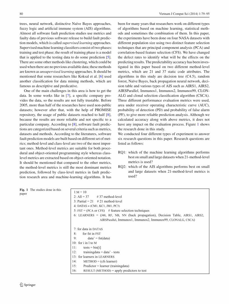
Fig. 2 The activity diagram ofAIRS algorithm

tasks to identify and prevent attacks from intrusions. There-fore, the artificial cells are equipped with the same attributesas the human immune system. The artificial cells try to modelthe behavior of the immune-cells of the human immune sys-tem. Network security, optimization problems and distrib-uted computing are some of the AIS’s applications.

There are several classifiers available based on AIS para-digm, some of them are as follows: AIRS, CLONALG, andIMMUNOS81, each one of them is reviewed in the followingsubsections.

3.1 Artificial intelligence recognition system (AIRS)

Artificial intelligence recognition system is one of the firstAIS techniques designed specifically and applied to classi-fication problems. It is a novel immune inspired supervisedlearning algorithm [28,29].

AIRS has five steps: initialization, antigen training, com-petition for limited resources, memory cell selection and clas-sification [4,27]. These five steps are summarized in Fig. 2.

First, the dataset is normalized, and then based on theEuclidian formula distances between antigens, which iscalled affinity, are calculated. Affinity threshold that is theuser-defined value is calculated. Antibodies that are presentin the memory pool are stimulated with a specific infectedantigen, and the stimulated value is assigned to each cell.The cell, which has the highest stimulation value, is chosenas the finest memory cell. Afterwards, the best match fromthe memory pool is selected and added to the artificial recog-nition ball (ARB) pool. This pool contains both antigen andantibodies with their stimulation value along with some otherinformation related to them. Next, the numbers of clones are

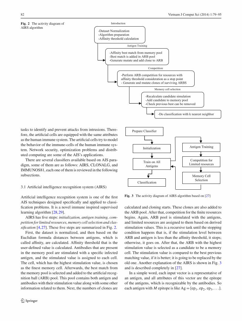
Fig. 3 The activity diagram of AIRS algorithm based on [27]

calculated and cloning starts. These clones are also added tothe ARB pool. After that, competition for the finite resourcesbegins. Again, ARB pool is stimulated with the antigens,and limited resources are assigned to them based on derivedstimulation values. This is a recursive task until the stoppingcondition happens that is, if the stimulation level betweenARB and antigen is less than the affinity threshold, it stops;otherwise, it goes on. After that, the ARB with the higheststimulation value is selected as a candidate to be a memorycell. The stimulation value is compared to the best previousmatching value, if it is better; it is going to be replaced by theold one. Another explanation of the AIRS is shown in Fig. 3and is described completely in [27].

In a simple word, each input vector is a representative ofan antigen, and all attributes of this vector are the epitopeof the antigens, which is recognizable by the antibodies. Soeach antigen with M epitope is like Ag = [ep1, ep2, ep3, . . .].

123

Vietnam J Comput Sci (2014) 1:79–95 83

For each epitope, one antibody is considered (Ab). Theaffinity between each pair of epitope of each antigen andantibody is calculated in Eqs. 1 and 2 as follows:

dist =√√√√

n∑

i=1

(v1i − v2i )2 (1)

Affinity = 1 − dist (Abk, epk) (2)

AIRSv1 is the first version of this algorithm. AIRSv1 (AIRS1)treats the ARB pool as a persistent resource during the entiretraining process whereas ARB pool is used as a temporaryresource for each antigen in AIRSv2 (AIRS2). In anotherword, ARB’s leftovers for past antigens from the previousARB refinement step are maintained and are participated ina competition for limited resources. According to [28] thiscause more time spending in rewarding and refining ARBsthat belong to the same class of the antigen in question. Inorder to solve this problem, a user defined stimulation valueis raised in AIRS2 and only clones of the same class as theantigen are considered in ARB pool. The other differencebetween these two algorithms is how mutation is done. InAIRS1, the mutate rate is a user defined parameter and showsthe mutate degree for producing a clone; mutate rate is simplyreplaced with normalized randomly generated value. Mutaterate in AIRS2 is identified as proportional to its affinity toantigen in question. This approach performs a better searchwhen there is a tight affinity. Both AIRS1 and AIRS2 showsimilar accuracy performance behavior except that, AIRS2is a simpler algorithm and is also show better generalizationcapability in terms of improved data reduction of the trainingdataset [4,27]. Watkins [29] introduced the parallel imple-mentation in 2005. The model shows the distributed natureand parallel processing attributes exhibited in mammalianimmune system. The approach is simple and we have to addthe following step to the standard AIRS training schema. Ifthe dataset is not partitioned too widely, then the trainingspeed is observable. AIRS Parallel have the following steps[4,27,29]:

• Divide the training dataset into np2 partitions.• Allocate training partitions to processes.• Combine np number of memory pools.• Use a merging approach to create the combined memory

pool.

Acceptance of continuous and nominal variables, capacityto learn and recall large numbers of patterns, experienced-based learning, supervised learning, classification accuracy,user parameter and the ability to predict the training times aresome of the design goals that could be noted for an AIRS-likesupervised learning system.

2 np is the number of partitions.

3.2 CLONALG

The theory specifies that the organism has a pre-existing poolof heterogeneous antibodies that can recognize all antigenswith some level of specificity [30].

As you may see in Fig. 4, when matching occurs, the can-didate cell undergoes mitosis and produces B lymphoblastthat could be one of the following:

• Plasma cell that produces antibody as an effector of theimmune response.

• Long-lived memory cell, in case a similar antigen appears.

CLONal selection ALGorithm is inspired by the clonalselection theory of acquired immunity, previously known asCSA. A new clonal selection inspired classification algorithmis called CSCA.

CLONALG inspires some features from clonal selectiontheory, which is mentioned above. The goal here is to developa memory pool containing best antigen matching antibodiesthat represent a solution to engineering problems.

The algorithm provides two searching mechanism for thedesired final pool of memory antibodies. These two are notedin [30] as follows:

• Local search, provided via affinity maturation of clonedantibodies. More clones are produced for better-matchedantibodies.

• A search that provides a global scope and involves theinsertion of randomly generated antibodies to be insertedinto the population to further increase the diversity andprovide a means for potentially escaping local optima.

Figure 5 shows an algorithm based on GLONALG The-ory. A CLONALG technique has a lower complexity andsmaller number of user parameters compared to other AISsystems such as AIRS [31]. CLONALG algorithm is mainlyused in three engineering problem domains: pattern recogni-tion, function optimization and combinatorial optimization[30].

Parallel CLONALG works like a distributed system. Theproblem is divided into number of processes. The task ofeach one is preparation of themselves as antigen pools. Aftercompletion, all results will be sent to the root and the memorypool forms based on the combination of them.

There are some other classifications based on clonal selec-tion algorithms such as CLONCLAS (CLONal selectionalgorithm for CLASsification) which is mostly used in char-acter recognition. Here, there is a concept called class thatcontains an antibody and the antigen exposed to a class ofspecific antibody.

To improve and maximize the accuracy of the classifica-tion and also minimize the wrong classification, CSCA cameto the picture. CSCA or clonal selection classifier algorithm

123

84 Vietnam J Comput Sci (2014) 1:79–95

Fig. 4 The simple overview ofthe clonal selection process,image taken from [32]

Fig. 5 Overview of theCLONALG algorithm

has four distinct steps, which is started with Initialization likeevery other AIS algorithm followed by repetition (loop) ofSelection and Pruning, Cloning and Mutation and Insertionuntil the stopping point, and at the end it has Final Pruningand Classification.

In Initialization step, an antibody pool is created based onrandomly selected antigen which has size S. In loop phase,there is a Selection and Pruning step that shows and scor-ing the antibody pool to each antigen set, which could beeither correct classification score or misclassification score.After that selection rules are applied, antibodies with a mis-classification score of zero are eliminated or antibodies with

the fitness scoring of less than epsilon are removed from thechosen set and from the original antibody set as well. Afterthat, all remaining antibodies in the selected set are cloned,mutated, and inserted to the main antibody set. When theloop condition is fulfilled, the Final Pruning step starts whichexposes the final antibodies set to each antigen and calculatesfitness scoring exactly like the loop step. Finally, the set ofexemplar is ready in antibody set, so in case of any unclassi-fied data instances that are exposed to the antibodies set, theaffinities between each matches are calculated and selectedand according to this result, unclassified data set could beclassified. Figure 6 shows the CSCA steps.

123

Vietnam J Comput Sci (2014) 1:79–95 85

Fig. 6 Overview of the CSCA algorithm taken from [30]

3.3 Immunos81

Most of the issues that described in AIS are close to bio-logical metaphor but the goal for Immunos81 is to reducethis part and focus on the practical application. Some of theterminologies are listed as below:

• T-Cell, both partitioning learned information and decisionsabout how new information is exposed to the system are

the duty of this cell, each specific antigen has a T-Cell, andit has one or more groups of B-Cells.

• B-Cell, there is an instance of a group of antigens.• Antigen, this is a defect; it has a data vector of attributes

where the nature of each attribute like name and data typeis known.

• Antigen-Type, depends on the domain, antigens are iden-tified by their names and series of attributes, which is aduty of T-Cell.

• Antigen group/clone based on the antigen’s type or a spe-cific classification label forms a group that is called cloneof B-Cell and as mentioned above, are controlled by aT-Cell.

• The recognition part of the antibody is called paratope,which is bound to the specific part of the antigen, epitopes(attributes of the antigen).

This algorithm has three main steps: initialization, trainingand classification [33]; the general idea behind the Immu-nos81 is shown in Fig. 7.

To calculate the affinity values for each paratope across allB-Cells, Eq. 3 is used, pi is the paratope affinity for the i thparatope, k is a scale factor and S is total number of B-Cell,

Fig. 7 Generalized version ofthe Immunos81 training scheme

Cla

ssif

icat

ion

step

Tra

ining

step

123

86 Vietnam J Comput Sci (2014) 1:79–95

j th B-Cell affinity in a clone set is shown by ai .

pai = k ·j=1∑

S

a j (3)

There is another concept called Avidity, which is sum ofaffinity values scaled both by the size of the clone populationand additional scale parameter, according to Eq. 4, ca is aclone avidity for the i th, k2i defines by user, N is the totalparatopes and total number of B-Cells in the i th clone set isshown by Si .

cai = k2i ·⎛

⎝

j=1∑

N

pa j

⎞

⎠ · Si (4)

There are two basic implementations for Immunos8 that areknown as naïve immunos algorithms; they are called,Immunos1 and Immunos2. There is no data reduction inImmunos1, and it is similar to the k-nearest neighbors. Theprimary difference is obviously that the training populationis partitioned and k is set to one for each partition; multiple-problem support can be provided with simpler mechanismthat uses classifier for each problem, and each classifier hasits own management mechanism. The Immunos2 implemen-tation is the same as Immunos1 only seeks to provide someform of primary generalization via data reduction, so thecloser representation to basic Immunos [33].

Immunos99 could be identified as a combination of Immu-nos81 and CSCA which some user-defined parameters areeither fixed or removed from the CSCA. Immunos99 is verydifferent from the AIR classifiers such as AIRS and CLON-ALG; they all do competition in a training phase so the sizeof the group set has some affection on affinity and avid-ity calculation. There is another distinguishing point also;there is a single exposure to the training set (only in CLON-ALG).

As mentioned before, there is a classification calledantigen-group and antigen-type. If the algorithm could iden-tify some groups of B-Cell that are able to identify a specifictype of antigens which these antigens might be also in differ-ent forms, then we can conclude that, how well any B-Cellscould respond to its designed class of antigens compared toany other classes. The training step is composed of four basiclevels; first data is divided into antigen-groups, and then theB-Cell population is set for each antigen-group (same as theimmunos). For user, defined number of times, the B-Cell isshown to the antigens from all groups and fitness value iscalculated; population pruning is done after that, two affinitymaturations based on cloning and mutations are performedand some random selected antigens from the same groupare inserted to the set. The loop is finished here when it isfulfilled the stopping condition. After last pruning for each B-Cell population, the final B-Cell population is introduced as

a classifier. The usefulness or fitness formula for each B-Cellis shown in Eq. 5.

Fitness = Correct

Incorrect(5)

Correct means, sum of antigen ranked based score of thesame group and incorrect means, sum of them in differentgroups of B-Cell. Here, all B-Cells have correct and incor-rect scores, and also the antigen-group could not be changed;this is different from CSCA method.

4 Feature selection

Feature selection identifies and extracts the most useful fea-tures of the dataset for learning, and these features are veryvaluable for analysis and future prediction. So by removingless important and redundant data, the performance of learn-ing algorithm could be improved. The nature of the trainingdata plays the major role in classification and prediction. Ifthe data fail to exhibit the statistical regularity that machinelearning algorithms exploit, then learning will fail, so oneof the important tasks here is removing the redundant datafrom the training set; it will, afterwards make the process ofdiscovering regularity much easier, faster and more accurate.

According to [34], Feature selection has four differentcharacteristics which are starting point, search organization,evaluation strategy, and stopping criterion. Starting pointmeans from where the research should begin, it could beeither begin with no feature and add a feature as you pro-ceed forward, or it could be a backward process; you startwith all attributes, and as you proceed, you do the featureelimination, or it could start from somewhere in the middleon the training set. In search organization step, suppose thedataset has N number of features, so there will be 2 N num-ber of subsets. So the search could be either exhausted orheuristic.

Evaluation strategy is divided into two main categories,which are wrapper, and filters. Wrapper evaluated the impor-tance of the features based on the learning algorithm, whichcould be applied on data later. It uses the search algorithmto search the entire feature’s population, run the model onthem, and evaluate each subset based on that model. Thistechnique could be computationally expensive; it has beenseen that it may have suffered from over fitting to the model.Cross validation is being used to estimate the final accu-racy of the feature subset. The goal of cross-validation is toestimate the expected level of fit of a model to a data setthat is independent of the data, which were used to train themodel. In filters, the evaluation is being done based on heuris-tic’s data and general characteristics of the data come to thepicture. Searching algorithm in both techniques are similarbut filter is faster and more practical when the populations

123

Vietnam J Comput Sci (2014) 1:79–95 87

of the features are high because the approach is based ongeneral characteristic of heuristic data rather than a methodwith a learning algorithm to evaluate the merit of a featuresubset.

Feature selection algorithms typically fall into two cate-gories; it could be either feature ranking or subset ranking.If the ranking is done based on metric and all features thatdo not achieve a sufficient score are removed, it is called fea-ture ranking but subset selection searches the set of possiblefeatures for the optimal subset, which includes wrapper andfilter.

4.1 Principal component analysis

Principal component analysis is a mathematical procedure,the aim of which is reducing the dimensionality of the dataset.It is also called an orthogonal linear transformation that trans-forms the data to a new coordinate system. In fact, PCA isa feature extraction technique rather than a feature selectionmethod. The new attributes are obtained by a linear combi-nation of the original attributes. Here, the features with thehighest variance are kept to do the reduction. Some paperslike [35] used PCA for improving their experiments’ perfor-mance. According to [36], the PCA technique transforms nvector {x1, x2, . . . , xn} from the d-dimensional space to nvectors {x ′

1, x ′2, . . . , x ′

n} in a new d ′ dimensional space.

x ′i =

d ′∑

k=1

ak,iek, d ′ ≤ d, (6)

where ek are eigenvectors corresponding to d ′ largest eigenvectors for the scatter matrix S and ak,i are the projections(principal components original data sets) of the original vec-tors xi on the eigenvectors ek .

4.2 Correlation-based feature selection

Correlation-based feature selection is an automatic algori-thm, which does not need user-defined parameters like thenumber of features that need to be selected. CFS is catego-rized aa filter.

According to [37], feature Vi is said to be relevant, If thereexists some vi and c for which p (Vi = vi ) > 0 such that inEq. 7.

p(C = c|Vi = vi ) �= p(C = c) (7)

According to research on feature selection experiments, irrel-evant features should be removed along with redundant infor-mation. A feature is said to be redundant if one or more ofthe other features are highly correlated with it [38]. As it wasmentioned before, all redundant attributes should be elimi-nated, so if any features’ prediction ability could be covered

by another, then it can be removed. CFS computes a heuris-tic measure of the “merit” of a feature subset from pair-wisefeature correlations and a formula adapted from test theory.Heuristic search is used to traverse the space of feature sub-sets in reasonable time; the subset with the highest meritfound during the search is reported. This method also needsdiscretizing the continuous features.

5 Experiment description

5.1 Dataset selection

Here, four datasets from REPOSITORY of NASA [39,40]are selected. These datasets are different in number of rowsand rate of defects. The largest dataset is JM1 with 10,885rows, which belongs to real time predictive ground systemproject; 19 % of these data are defected. The smallest dataset,CM1, belongs to NASA spacecraft instrument project and ithas 498 modules and 10 % of the data are defected. KC1is another dataset which belongs to storage managementproject for receiving and processing ground data with 2,109modules. 15 % of the KC1 modules are defected. PC3 is thelast dataset that has 1,563 modules; 10 % of the data aredefected and it belongs to flight software for earth orbitingsatellite [39]. It should mention that PC3 is used only in firsttwo experiments.

5.2 Variable selection

Predictability performance is calculated based on two distinctmethod-level metrics 21 and 37. In this work, experimentsthat have not been performed in [4] are studied. All 21 met-rics which are the combination of McCabe’s and Halstead’sattributes are listed in Table 1. McCabe’s and Halstead’s met-rics are called module or method level metrics and the faultyor non-faulty label is assigned to each one of the modules.These set of metrics are also called static code attributes andaccording to [13] they are useful, easy to use and widely used.Most of these static codes could be collected easily, cheaplyand automatically. Many researchers and verification and val-idation text books such as [13,41] suggest using complexitymetrics to decide about which module is worthy of man-ual inspection. NASA researchers like Menzies et al. [13]with lots of experience about large governmental softwarehave declared that they will not review software modulesunless tools like McCabe predict that they are fault prone.Nevertheless, some researchers such as Shepperd and Ince[42] and Fenton and Pfleeger [43] argued that static codessuch as McCabe are useless metrics, but Menzies et al. in[13,20] proved that prediction based on the selected datasetwith static code metrics performed very well and based ontheir studies they built prediction model with higher proba-

123

88 Vietnam J Comput Sci (2014) 1:79–95

Table 1 Attributes present in 21 method-level metrics [39,40]

Attributes names Information

loc McCabe’s line count of code

v(g) McCabe “cyclomatic complexity”

ev(g) McCabe “essential complexity”

iv(g) McCabe “design complexity”

n Halstead total operators + operands

v Halstead “volume”

l Halstead “program length”

d Halstead “difficulty”

i Halstead “intelligence”

e Halstead “effort”

b Halstead “delivered bugs”

t Halstead’s time estimator

lOCode Halstead’s line count

lOComment Halstead’s count of lines of comments

lOBlank Halstead’s count of blank lines

lOCodeAndlOComment Lines of code and comments

uniq_op Unique operators

uniq_opnd Unique operands

total_op Total operators

total_opnd Total operand

branchCount Branch count of the flow graph

bility of detection and lower probability of false alarm whichwas in contrast with Shepherd and Ince [42] and Fenton andPfleeger [43] beliefs.

As it is shown in Table 1, the attributes mainly consist oftwo different types, McCabe and Halstead. McCabe arguedthat codes with complicated pathways are more error-prone.His metrics, therefore, reflects the pathways within a codemodule but Halstead argued that, code that is hard to read, ismore likely to be fault prone.

5.3 Simulator selection

All the experiments have been done in WEKA, which is open-source software and implemented in JAVA; it is developed inthe University of Waikato and it is used for machine learningstudies [44].

5.4 Performance measurements criteria

We used tenfold cross validations and all experiments wererepeated five times. According to Menzies et al. [13,20] sincesome models with low precision performed well, using itas a reliable parameter for performance evaluation is notgood. They also mentioned that if the target class (faulty/non-faulty) is in the minority, accuracy is a poor measure as forexample, a classifier could score 90 % accuracy on a dataset

Table 2 Confusion matrix

No (predicted) Yes (predicted)

No (actual) TN FP

Yes (actual) FN TP

with 10 % faulty data, even if it predicts that all defectivemodules are defect free. Hence in this study, area underreceiver operating characteristic curve values were used forbenchmarking especially when the dataset is unbalanced.Other performance evaluation metrics that were used are:PD which is the number of fault-prone modules that are clas-sified correctly and PF that is the number of not fault-pronemodules that are classified incorrectly as defected, Table 2,Eqs. 8, 9 and 10 show all details about calculation of perfor-mance evaluation metrics. As a brief explanation, true neg-ative (TN) means that the module is predicted as non-faultycorrectly, whereas false negative (FN) means that the moduleis predicted as non-faulty wrongly. On the other hand, falsepositive (FP) means that the module is estimated as faultyincorrectly and true positive (TP) denotes that the module ispredicted as faulty correctly.

Accuracy = TP + TN

TP + FN + FP + TN(8)

Recall(PD) = TP

TP + FN(9)

PF = FP

FP + TN(10)

6 Analysis of the experiment

6.1 Experiment 1

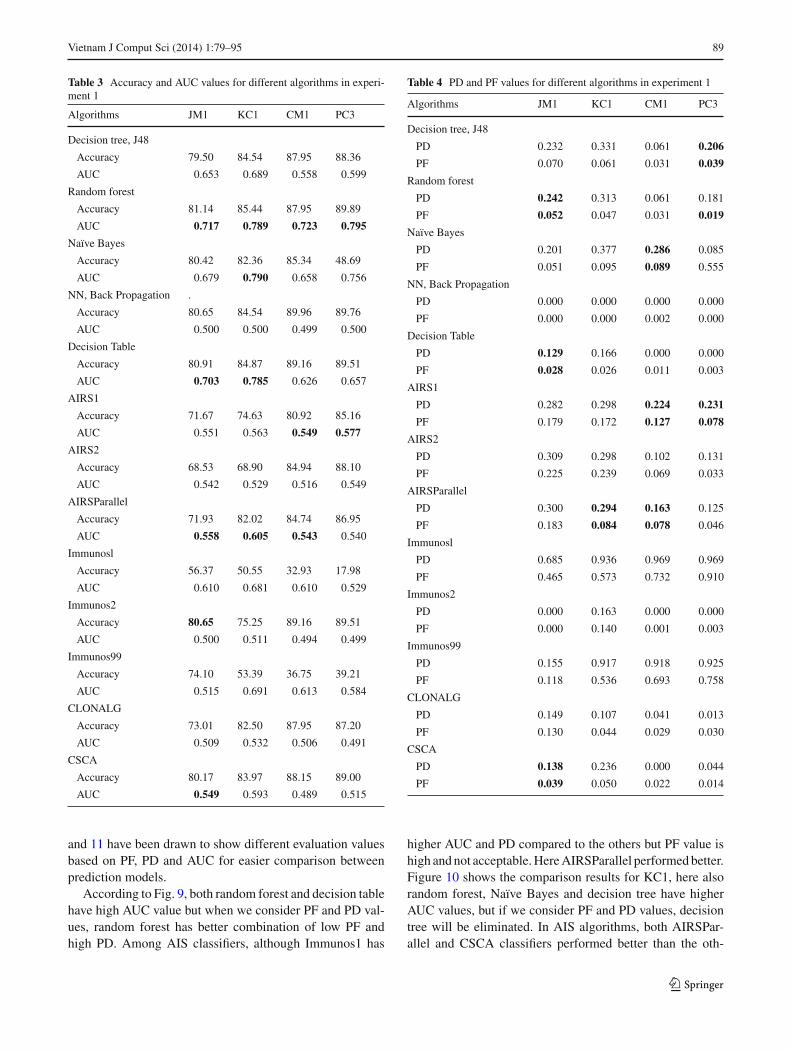
Twenty-one method-level metrics were used for this exper-iment. All 13 machine-learning techniques were applied onfour different NASA datasets, and the results were com-pared. Table 3 shows accuracy and AUC value of algorithmsand Table 4 presents PD and PF values for this experiment.This experiment has been done to answer research question 1and 2. Notable values obtained after applying each algorithmare specified in bold.

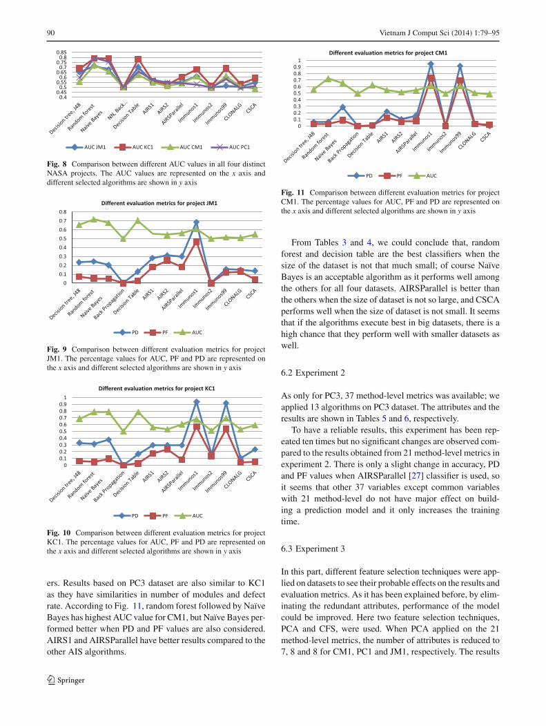
As mentioned earlier and according to Menzies et al.[13,20], a good prediction should have high AUC and PDvalues as well as low PF value, so with this consideration,we have evaluated the results. Figure 8 presents the perfor-mance comparison in terms of AUC among four differentNASA projects. According to the figure, both random forestand decision table performed best compared to other algo-rithms for JM1. For KC1, Naïve Bayes also performed wellalong with random forest and decision table. Random forestperformed best when it comes to CM1 as well. Figures 9, 10

123

Vietnam J Comput Sci (2014) 1:79–95 89

Table 3 Accuracy and AUC values for different algorithms in experi-ment 1

Algorithms JM1 KC1 CM1 PC3

Decision tree, J48

Accuracy 79.50 84.54 87.95 88.36

AUC 0.653 0.689 0.558 0.599

Random forest

Accuracy 81.14 85.44 87.95 89.89

AUC 0.717 0.789 0.723 0.795

Naïve Bayes

Accuracy 80.42 82.36 85.34 48.69

AUC 0.679 0.790 0.658 0.756

NN, Back Propagation .

Accuracy 80.65 84.54 89.96 89.76

AUC 0.500 0.500 0.499 0.500

Decision Table

Accuracy 80.91 84.87 89.16 89.51

AUC 0.703 0.785 0.626 0.657

AIRS1

Accuracy 71.67 74.63 80.92 85.16

AUC 0.551 0.563 0.549 0.577

AIRS2

Accuracy 68.53 68.90 84.94 88.10

AUC 0.542 0.529 0.516 0.549

AIRSParallel

Accuracy 71.93 82.02 84.74 86.95

AUC 0.558 0.605 0.543 0.540

Immunosl

Accuracy 56.37 50.55 32.93 17.98

AUC 0.610 0.681 0.610 0.529

Immunos2

Accuracy 80.65 75.25 89.16 89.51

AUC 0.500 0.511 0.494 0.499

Immunos99

Accuracy 74.10 53.39 36.75 39.21

AUC 0.515 0.691 0.613 0.584

CLONALG

Accuracy 73.01 82.50 87.95 87.20

AUC 0.509 0.532 0.506 0.491

CSCA

Accuracy 80.17 83.97 88.15 89.00

AUC 0.549 0.593 0.489 0.515

and 11 have been drawn to show different evaluation valuesbased on PF, PD and AUC for easier comparison betweenprediction models.

According to Fig. 9, both random forest and decision tablehave high AUC value but when we consider PF and PD val-ues, random forest has better combination of low PF andhigh PD. Among AIS classifiers, although Immunos1 has

Table 4 PD and PF values for different algorithms in experiment 1

Algorithms JM1 KC1 CM1 PC3

Decision tree, J48

PD 0.232 0.331 0.061 0.206

PF 0.070 0.061 0.031 0.039

Random forest

PD 0.242 0.313 0.061 0.181

PF 0.052 0.047 0.031 0.019

Naïve Bayes

PD 0.201 0.377 0.286 0.085

PF 0.051 0.095 0.089 0.555

NN, Back Propagation

PD 0.000 0.000 0.000 0.000

PF 0.000 0.000 0.002 0.000

Decision Table

PD 0.129 0.166 0.000 0.000

PF 0.028 0.026 0.011 0.003

AIRS1

PD 0.282 0.298 0.224 0.231

PF 0.179 0.172 0.127 0.078

AIRS2

PD 0.309 0.298 0.102 0.131

PF 0.225 0.239 0.069 0.033

AIRSParallel

PD 0.300 0.294 0.163 0.125

PF 0.183 0.084 0.078 0.046

Immunosl

PD 0.685 0.936 0.969 0.969

PF 0.465 0.573 0.732 0.910

Immunos2

PD 0.000 0.163 0.000 0.000

PF 0.000 0.140 0.001 0.003

Immunos99

PD 0.155 0.917 0.918 0.925

PF 0.118 0.536 0.693 0.758

CLONALG

PD 0.149 0.107 0.041 0.013

PF 0.130 0.044 0.029 0.030

CSCA

PD 0.138 0.236 0.000 0.044

PF 0.039 0.050 0.022 0.014

higher AUC and PD compared to the others but PF value ishigh and not acceptable. Here AIRSParallel performed better.Figure 10 shows the comparison results for KC1, here alsorandom forest, Naïve Bayes and decision tree have higherAUC values, but if we consider PF and PD values, decisiontree will be eliminated. In AIS algorithms, both AIRSPar-allel and CSCA classifiers performed better than the oth-

123

90 Vietnam J Comput Sci (2014) 1:79–95

Fig. 8 Comparison between different AUC values in all four distinctNASA projects. The AUC values are represented on the x axis anddifferent selected algorithms are shown in y axis

Fig. 9 Comparison between different evaluation metrics for projectJM1. The percentage values for AUC, PF and PD are represented onthe x axis and different selected algorithms are shown in y axis

Fig. 10 Comparison between different evaluation metrics for projectKC1. The percentage values for AUC, PF and PD are represented onthe x axis and different selected algorithms are shown in y axis

ers. Results based on PC3 dataset are also similar to KC1as they have similarities in number of modules and defectrate. According to Fig. 11, random forest followed by NaïveBayes has highest AUC value for CM1, but Naïve Bayes per-formed better when PD and PF values are also considered.AIRS1 and AIRSParallel have better results compared to theother AIS algorithms.

Fig. 11 Comparison between different evaluation metrics for projectCM1. The percentage values for AUC, PF and PD are represented onthe x axis and different selected algorithms are shown in y axis

From Tables 3 and 4, we could conclude that, randomforest and decision table are the best classifiers when thesize of the dataset is not that much small; of course NaïveBayes is an acceptable algorithm as it performs well amongthe others for all four datasets. AIRSParallel is better thanthe others when the size of dataset is not so large, and CSCAperforms well when the size of dataset is not small. It seemsthat if the algorithms execute best in big datasets, there is ahigh chance that they perform well with smaller datasets aswell.

6.2 Experiment 2

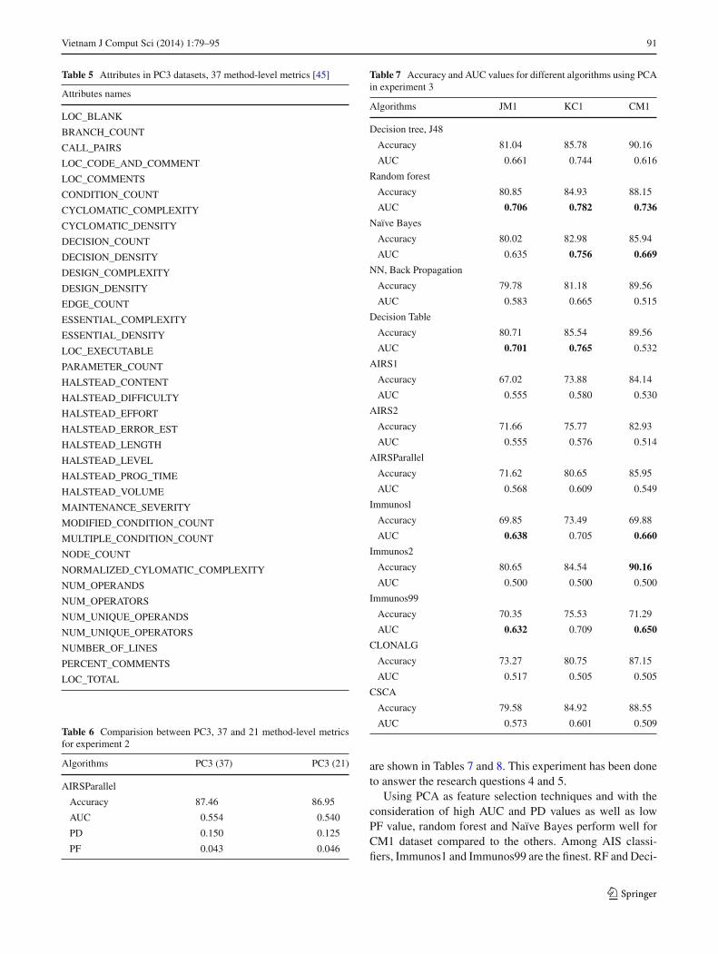
As only for PC3, 37 method-level metrics was available; weapplied 13 algorithms on PC3 dataset. The attributes and theresults are shown in Tables 5 and 6, respectively.

To have a reliable results, this experiment has been rep-eated ten times but no significant changes are observed com-pared to the results obtained from 21 method-level metrics inexperiment 2. There is only a slight change in accuracy, PDand PF values when AIRSParallel [27] classifier is used, soit seems that other 37 variables except common variableswith 21 method-level do not have major effect on build-ing a prediction model and it only increases the trainingtime.

6.3 Experiment 3

In this part, different feature selection techniques were app-lied on datasets to see their probable effects on the results andevaluation metrics. As it has been explained before, by elim-inating the redundant attributes, performance of the modelcould be improved. Here two feature selection techniques,PCA and CFS, were used. When PCA applied on the 21method-level metrics, the number of attributes is reduced to7, 8 and 8 for CM1, PC1 and JM1, respectively. The results

123

Vietnam J Comput Sci (2014) 1:79–95 91

Table 5 Attributes in PC3 datasets, 37 method-level metrics [45]

Attributes names

LOC_BLANK

BRANCH_COUNT

CALL_PAIRS

LOC_CODE_AND_COMMENT

LOC_COMMENTS

CONDITION_COUNT

CYCLOMATIC_COMPLEXITY

CYCLOMATIC_DENSITY

DECISION_COUNT

DECISION_DENSITY

DESIGN_COMPLEXITY

DESIGN_DENSITY

EDGE_COUNT

ESSENTIAL_COMPLEXITY

ESSENTIAL_DENSITY

LOC_EXECUTABLE

PARAMETER_COUNT

HALSTEAD_CONTENT

HALSTEAD_DIFFICULTY

HALSTEAD_EFFORT

HALSTEAD_ERROR_EST

HALSTEAD_LENGTH

HALSTEAD_LEVEL

HALSTEAD_PROG_TIME

HALSTEAD_VOLUME

MAINTENANCE_SEVERITY

MODIFIED_CONDITION_COUNT

MULTIPLE_CONDITION_COUNT

NODE_COUNT

NORMALIZED_CYLOMATIC_COMPLEXITY

NUM_OPERANDS

NUM_OPERATORS

NUM_UNIQUE_OPERANDS

NUM_UNIQUE_OPERATORS

NUMBER_OF_LINES

PERCENT_COMMENTS

LOC_TOTAL

Table 6 Comparision between PC3, 37 and 21 method-level metricsfor experiment 2

Algorithms PC3 (37) PC3 (21)

AIRSParallel

Accuracy 87.46 86.95

AUC 0.554 0.540

PD 0.150 0.125

PF 0.043 0.046

Table 7 Accuracy and AUC values for different algorithms using PCAin experiment 3

Algorithms JM1 KC1 CM1

Decision tree, J48

Accuracy 81.04 85.78 90.16

AUC 0.661 0.744 0.616

Random forest

Accuracy 80.85 84.93 88.15

AUC 0.706 0.782 0.736

Naïve Bayes

Accuracy 80.02 82.98 85.94

AUC 0.635 0.756 0.669

NN, Back Propagation

Accuracy 79.78 81.18 89.56

AUC 0.583 0.665 0.515

Decision Table

Accuracy 80.71 85.54 89.56

AUC 0.701 0.765 0.532

AIRS1

Accuracy 67.02 73.88 84.14

AUC 0.555 0.580 0.530

AIRS2

Accuracy 71.66 75.77 82.93

AUC 0.555 0.576 0.514

AIRSParallel

Accuracy 71.62 80.65 85.95

AUC 0.568 0.609 0.549

Immunosl

Accuracy 69.85 73.49 69.88

AUC 0.638 0.705 0.660

Immunos2

Accuracy 80.65 84.54 90.16

AUC 0.500 0.500 0.500

Immunos99

Accuracy 70.35 75.53 71.29

AUC 0.632 0.709 0.650

CLONALG

Accuracy 73.27 80.75 87.15

AUC 0.517 0.505 0.505

CSCA

Accuracy 79.58 84.92 88.55

AUC 0.573 0.601 0.509

are shown in Tables 7 and 8. This experiment has been doneto answer the research questions 4 and 5.

Using PCA as feature selection techniques and with theconsideration of high AUC and PD values as well as lowPF value, random forest and Naïve Bayes perform well forCM1 dataset compared to the others. Among AIS classi-fiers, Immunos1 and Immunos99 are the finest. RF and Deci-

123

92 Vietnam J Comput Sci (2014) 1:79–95

Table 8 PD and PF values for different algorithms using PCA in exper-iment 3

Algorithms JM1 KC1 CM1

Decision tree, J48

PD 0.096 0.239 0.041

PF 0.018 0.029 0.004

Random forest

PD 0.235 0.267 0.041

PF 0.054 0.045 0.027

Naïve Bayes

pd 0.195 0.337 0.224

PF 0.055 0.080 0.071

NN, Back Propagation

PD 0.224 0.451 0.000

PF 0.056 0.121 0.007

Decision Table

PD 0.101 0.166 0.041

PF 0.024 0.019 0.011

AIRS1

PD 0.366 0.350 0.143

PF 0.257 0.190 0.082

AIRS2

PD 0.291 0.313 0.122

PF 0.181 0.161 0.094

AIRSParallel

PD 0.326 0.319 0.163

PF 0.019 0.100 0.065

Immunosl

PD 0.540 0.663 0.612

PF 0.264 0.252 0.292

Immunos2

PD 0.000 0.000 0.000

PF 0.000 0.000 0.000

Immunos99

PD 0.516 0.641 0.571

PF 0.251 0.224 0.272

CLONALG

PD 0.166 0.067 0.041

PF 0.133 0.057 0.038

CSCA

PD 0.211 0.242 0.041

PF 0.064 0.040 0.022

sion Table are best for both JM1 and KC1 datasets withAUC, PD and PF as a performance evaluation metrics; alsoImmunos99 performs best among the other AIS algorithmsfor JM1.

After applying CFS with the best first classifier, some ofthe attributes were eliminated from the 21 of total attributes;seven attributes remain from CM1, eight from KC1 and JM1.

Table 9 Accuracy and AUC values for different algorithms using CFS,Best First in experiment 3

Algorithms JM1 KC1 CM1

Decision tree, J48

Accuracy 81.01 84.68 89.31

AUC 0.664 0.705 0.542

Random forest

Accuracy 80.28 84.83 88.15

AUC 0.710 0.786 0.615

Naïve Bayes

Accuracy 80.41 82.41 86.55

AUC 0.665 0.785 0.691

NN, Back Propagation

Accuracy 80.65 84.54 90.16

AUC 0.500 0.500 0.500

Decision Table

Accuracy 80.81 84.92 89.16

AUC 0.701 0.781 0.626

AIRS1

Accuracy 66.76 76.34 84.54

AUC 0.567 0.602 0.569

AIRS2

Accuracy 73.36 77.34 82.53

AUC 0.565 0.591 0.530

AIRSParallel

Accuracy 70.17 79.47 86.14

AUC 0.564 0.588 0.488

Immunos1

Accuracy 59.99 49.98 69.88

AUC 0.600 0.678 0.697

Immunos2

Accuracy 80.65 80.23 90.16

AUC 0.500 0.491 0.500

Immunos99

Accuracy 65.02 62.21 76.51

AUC 0.594 0.705 0.679

CLONALG

Accuracy 72.92 79.28 87.95

AUC 0.512 0.522 0.497

CSCA

Accuracy 79.55 83.21 87.75

AUC 0.575 0.590 0.505

The results are also shown in Tables 9 and 10. The remainingattributes form JM1, KC1 and CM1 after applying CFS, bestfirst are listed below:

CM1: loc, iv(g), i, LOComment, LOBlank, uniq_Op, Uniq_Opnd

123

Vietnam J Comput Sci (2014) 1:79–95 93

Table 10 PD and PF values for different algorithms using CFS, BestFirst in experiment 3

Algorithms JM1 KC1 CM1

Decision tree, J48

PD 0.148 0.175 0.000

PF 0.031 0.030 0.009

Random forest

PD 0.243 0.282 0.102

PF 0.063 0.048 0.033

Naïve Bayes

pd 0.223 0.365 0.306

PF 0.056 0.092 0.073

NN, Back Propagation

pd 0.000 0.000 0.000

PF 0.000 0.000 0.000

Decision Table

PD 0.108 0.178 0.000

PF 0.024 0.028 0.011

AIRS1

PD 0.402 0.368 0.224

PF 0.269 0.184 0.087

AIRS2

PD 0.290 0.328 0.163

PF 0.160 0.145 0.102

AIRSParallel

PD 0.301 0.301 0.041

PF 0.173 0.125 0.065

Immunos1

PD 0.600 0.936 0.694

PF 0.400 0.058 0.301

Immunos2

PD 0.000 0.040 0.000

PF 0.000 0.058 0.000

Immunos99

PD 0.502 0.825 0.571

PF 0.314 0.415 0.214

CLONALG

PD 0.159 0.129 0.020

PF 0.134 0.086 0.027

CSCA

PD 0.217 0.239 0.041

PF 0.066 0.059 0.031

KC1: v, d, i, LOCode, LOComment, LOBlank, Uniq_Opnd, branchcout

JM1: loc, v(g), ev(g), iv(g), i, LOComment, LOBlank, loc-CodeAndComment

It should be mentioned here, after applying CFS, BestFirst, there are only slight changes observed in the results, soit means that there is no considerable difference in the results

after applying distinct feature selection techniques. The mainchange would be the execution time reduction. As it is shownin Tables 9 and 10, the best performance for JM1, which isthe largest dataset, belongs to decision tree followed by ran-dom forest. By checking the AUC, PF and PD values, naïvebayes perform greatly on CM1 dataset as well as the otherthree. CSCA also performed well among the other AIS clas-sifiers, but the problem with this algorithm is long executiontime.

We also applied CFS, random search to see whether it hasa considerable change in the results or not. It was found thatthere is no significant difference between selected attributesfor KC1 after applying feature selection methods. There wereonly six attributes selected for CM1, which is less than thebest first method. The number of selected attributes for JM1is increased by one compared to the best first as well. Sinceno noticeable differences observed in performance evalua-tion metrics after building prediction model based on CFS,random search, we do not show the results in this sec-tion. However, the remaining attributes from JM1, KC1 andCM1 after applying CFS, random search are presented asfollows:

CM1: loc, iv(g), i, b, LOComment, uniq_OpKC1: v, d, i, LOCode, LOComment, LOBlank, Uniq_

Opnd, branchcoutJM1: loc, v(g), ev(g), iv(g), n, i, LOComment, LOBlank,

locCodeAndComment

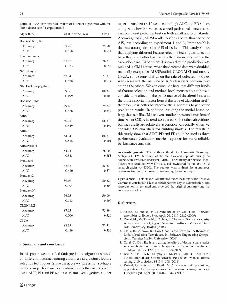
6.4 Experiment 4

As we noted earlier, each of these datasets has a differentrate of defected data; 19 % of the JM1, 10 % of the CM1 and15 % of KC1 are defected. So in this experiment, the rate ofdefected data was doubled in CM1 to identify whether any ofthe classifiers shows any distinctive changes in results com-pared to the previous trials; this experiment uses 21 method-level metrics to answer the research question 6. We show theresults in Table 11.

According to Table 11, the accuracy rate of all algorithmsis decreased except for Immunos1 and Immunos99. There-fore, it means that the findings could be a challenging factbecause it shows that the performance of each classifier couldtightly related to defect rate in the datasets. So previouslysuggested classifiers may not be the best choices anymoreto build a prediction model when the defect rate is changed.Accuracy in almost all the algorithms is fallen down, but ifwe consider AUC for evaluation, we see that this value growsin two other algorithms that are basically from one category,GLONALG and CSCA [30]. It could be concluded that byincreasing the defect rate, the artificial immune classifiersperform better and gives a finest prediction model comparedto others.

123

94 Vietnam J Comput Sci (2014) 1:79–95

Table 11 Accuracy and AUC values of different algorithms with dif-ferent defect rate for experiment 4

Algorithms CM1 (Old Values) CM1

Decision tree, J48

Accuracy 87.95 75.50

AUC 0.558 0.534

Random Forest

Accuracy 87.95 76.71

AUC 0.723 0.656

Naïve Bayes

Accuracy 85.34 77.31

AUC 0.658 0.614

NN, Back Propagation

Accuracy 89.96 80.32

AUC 0.499 0.500

Decision Table

Accuracy 89.16 79.72

AUC 0.626 0.554

AIRS1

Accuracy 80.92 66.27

AUC 0.549 0.497

AIRS2

Accuracy 84.94 68.67

AUC 0.516 0.501

AIRSParallel

Accuracy 84.74 76.10

AUC 0.543 0.555

Immunosl

Accuracy 32.92 38.35

AUC 0.610 0.574

Immunos2

Accuracy 89.16 80.32

AUC 0.494 0.500

Immunos99

Accuracy 36.75 50.00

AUC 0.613 0.600

CLONALG

Accuracy 87.95 73.69

AUC 0.506 0.520

CSCA

Accuracy 88.15 78.31

AUC 0.489 0.530

7 Summary and conclusion

In this paper, we identified fault prediction algorithms basedon different machine learning classifiers and distinct featureselection techniques. Since the accuracy rate is not a reliablemetrics for performance evaluation, three other metrics wereused, AUC, PD and PF which were not used together in other

experiments before. If we consider high AUC and PD valuesalong with low PF value as a well-performed benchmark,random forest performs best on both small and big datasets.According to [4], AIRSParallel performs better than the otherAIS, but according to experiment 1 and 3, Immunos99 isthe best among the other AIS classifiers. This study showsthat applying different feature selection techniques does nothave that much effect on the results; they mainly reduce theexecution time. Experiment 4 shows that the prediction ratereduced in CM1 dataset when the defected data were doubledmanually except for AIRSParallel, CLONALG and mostlyCSCA, so it seems that when the rate of defected moduleswas increased, the mentioned AIS classifiers perform bestamong the others. We can conclude here that different kindsof feature selection and method-level metrics do not have aconsiderable effect on the performance of the algorithm, andthe most important factor here is the type of algorithm itself;therefore, it is better to improve the algorithms to get betterprediction results. In addition, building the model based onlarge datasets like JM1 or even smaller ones consumes lots oftime when CSCA is used compared to the other algorithmsbut the results are relatively acceptable, especially when weconsider AIS classifiers for building models. The results inthis study show that AUC, PD and PF could be used as threeperformance evaluation metrics together for more reliableperformance analysis.

Acknowledgments The authors thank to Universiti TeknologiMalaysia (UTM) for some of the facilities and supports during thecourse of this research under vot 03H02. The Ministry of Science, Tech-nology & Innovation (MOSTI) is also acknowledged for supporting theresearch under vot 4S062. The authors wish to thank the anonymousreviewers for their comments in improving the manuscript.

Open Access This article is distributed under the terms of the CreativeCommons Attribution License which permits any use, distribution, andreproduction in any medium, provided the original author(s) and thesource are credited.

References

1. Zheng, J.: Predicting software reliability with neural networkensembles. J. Expert Syst. Appl. 36, 2116–2122 (2009)

2. Dowd, M., MC Donald, J., Schuh, J.: The Art of Software SecurityAssessment: Identifying & Preventing Software Vulnerabilities.Addison-Wesley, Boston (2006)

3. Clark, B., Zubrow, D.: How Good is the Software: A Review ofDefect Prediction Techniques. In: Software Engineering Sympo-sium, Carreige Mellon University (2001)

4. Catal, C., Diri, B.: Investigating the effect of dataset size, metricssets, and feature selection techniques on software fault predictionproblem. Inf. Sci. 179(8), 1040–1058 (2009)

5. Xie, X., Ho, J.W.K., Murphy, C., Kaiser, G., Xu, B., Chen, T.Y.:Testing and validating machine learning classifiers by metamorphictesting. J. Syst. Softw. 84, 544–558 (2011)

6. Koksal, G., Batmaz, I., Testik, M.C.: A review of data miningapplications for quality improvement in manufacturing industry.J. Expert Syst. Appl. 38, 13448–13467 (2011)

123

Vietnam J Comput Sci (2014) 1:79–95 95

7. Hewett, R.: Minig Software defect Data to Support Software testingManagement. Springer Science + Business Media, LLC, Berlin(2009)

8. Catal, C., Diri, B.: A systematic review of software fault prediction.J. Expert Syst. Appl. 36, 7346–7354 (2009)

9. Catal, C.: Software fault prediction: a literature review and currenttrends. J. Expert Syst. Appl. 38, 4626–4636 (2011)

10. Evett, M., Khoshgoftaar, T., Chien, P., Allen, E.: GP-based softwarequality prediction. In: Proceedings of the Third Annual GeneticProgramming Conference, San Francisco, CA, pp. 60–65 (1998)

11. Koprinska, I., Poon, J., Clark, J., Chan, J.: Learning to classifye-mail. Inf. Sci. 177(10), 2167–2187 (2007)

12. Thwin, M.M., Quah, T.: Application of neural networks for soft-ware quality prediction using object-oriented metrics. In: Proceed-ings of the 19th International Conference on Software Mainte-nance, Amsterdam, The Netherlands, pp. 113–122 (2003)

13. Menzies, T., Greenwald, J., Frank, A.: Data mining static codeattributes to learn defect predictors. IEEE Trans. Softw. Eng. 33(1),2–13 (2007)

14. El Emam, K., Benlarbi, S., Goel, N., Rai, S.: Comparing case-basedreasoning classifiers for predicting high risk software components.J. Syst. Softw. 55(3), 301–320 (2001)

15. Yuan, X., Khoshgoftaar, T.M., Allen, E.B., Ganesan, K.: An appli-cation of fuzzy clustering to software quality prediction. In: Pro-ceedings of the Third IEEE Symposium on Application-SpecificSystems and Software Engineering Technology. IEEE ComputerSociety, Washington, DC (2000)

16. Catal, C., Diri, B.: Software fault prediction with object-orientedmetrics based artificial immune recognition system. In: Proceed-ings of the 8th International Conference on Product Focused Soft-ware Process Improvement. Lecture Notes in Computer Science,pp. 300–314. Springer, Riga (2007)

17. Catal, C., Diri, B.: A fault prediction model with limited fault datato improve test process. In: Proceedings of the Ninth InternationalConference on Product Focused Software Process Improvements.Lecture Notes in Computer Science, pp. 244–257. Springer, Rome(2008)

18. Catal, C., Diri, B.: Software defect prediction using artificialimmune recognition system. In: Proceedings of the Fourth IASTEDInternational Conference on Software Engineering, pp. 285–290.IASTED, Innsburk (2007)

19. Zhang, H., Zhang, X.: Comments on data mining static codeattributes to learn defect predictors. IEEE Trans. Softw. Eng. (2007)

20. Menzies, T., Dekhtyar, A., Di Stefano, J., Greenwald, J.: Problemswith precision: a response to comments on data mining static codeattributes to learn defect predictors. IEEE Trans. Softw. Eng. 33(7),637–640 (2007)

21. Koru, G., Liu, H.: Building effective defect prediction models inpractice. IEEE Softw. 22(6), 23–29 (2005)

22. Shafi, S, Hassan, S.M., Arshaq, A., Khan, M.J., Shamail, S.: Soft-ware quality prediction techniques: a comparative analysis. In:Fourth International Conference on Emerging Technologies, pp.242–246 (2008)

23. Turhan, B., Bener, A.: Analysis of Naïve Bayes assumption onsoftware fault data: an empirical study. Data Knowl. Eng. 68(2),278–290 (2009)

24. Alsmadi, I., Najadat, H.: Evaluating the change of software faultbehavior with dataset attributes based on categorical correlation.Adv. Eng. Softw. 42, 535–546 (2011)

25. Sandhu, P.S., Singh, S., Budhija, N.: Prediction of level of severityof faults in software systems using density based clustering. In:2011 IEEE International Conference on Software and ComputerApplications. IPCSIT, vol. 9 (2011)

26. Turhan, B., Kocak, G., Bener, A.: Data mining source code forlocating software bugs; a case study in telecommunication industry.J. Expert Syst. Appl. 36, 9986–9990 (2009)

27. Brownlee, J.: Artificial immune recognition system: a review andanalysis. Technical Report 1–02, Swinburne University of Tech-nology (2005)

28. Watkins, A.: A Resource Limited Artificial Immune Classifier.Master’s thesis, Mississippi State University (2001)

29. Watkins, A.: Exploiting immunological metaphors in the develop-ment of serial, parallel, and distributed learning algorithms. PhDthesis, Mississippi State University (2005)

30. Brownlee, J.: Clonal selection theory & CLONALG. The clonalselection classification algorithm. Technical Report 2–02, Swin-burne University of Technology (2005)

31. Watkins, A., Timmis, J., Boggess, L.: Artificial Immune Recog-nition System (AIRS): An Immune-Inspired Supervised LearningAlgorithm. Genetic Programming and Evolvable Machines, vol. 5,pp. 291–317 (2004)

32. http://users.rcn.com/jkimball.ma.ultranet/BiologyPages/C/ClonalSelection.html. Retrieved 1 Nov 2013

33. Brownlee, J.: Immunos-81—The Misunderstood ArtificialImmune System. Technical Report 3–01. Swinburne University ofTechnology (2005)

34. Langley, P.: Selection of relevant features in machine learning. In:Proceedings of the AAAI Fall Symposium on Relevance. AAAIPress, California (1994)

35. Khoshgoftaar, T.M., Seliya, N., Sundaresh, N.: An empirical studyof predicting software faults with case-based reasoning. Softw.Qual. J. 14(2), 85–111 (2006)

36. Malhi, A.: PCA-Based feature selection scheme for machine defectclassification. IEEE Trans. Instrum. Meas. 53(6) (2004)

37. Kohavi, R., John, G.: Wrappers for feature subset selection. Artif.Intell. Special Issue Relev. 97(1–2), 273–324 (1996)

38. Hall, M.A.: Correlation-based Feature Subset Selection forMachine Learning. PhD dissertation, Department of Computer Sci-ence, University of Waikato (1999)

39. http://promise.site.uottawa.ca/SERepository/datasets. Retrieved01 Dec 2011

40. http://promisedata.org/?cat=5. Retrieved 01 Dec 201141. Rakitin, S.: Software Verification and Validation for Practitioners

and Managers, 2nd edn. Artech House, London (2001)42. Shepperd, M., Ince, D.: A critique of three metrics. J. Syst. Softw.

26(3), 197–210 (1994)43. Fenton, N.E., Pfleeger, S.: Software Metrics: A Rigorous and Prac-

tical Approach. Int’l Thompson Press, New York (1997)44. http://www.cs.waikato.ac.nz/ml/weka. Retrieved 01 Nov 201145. http://promisedata.org/repository/data/pc3/pc3.arff. Retrieved 01

Dec 2011

123