A Study of the Finite Sample Properties of

EMM, GMM, QMLE, and MLE for a

Square-Root Interest Rate Di�usion Model

Hao Zhou1

Mail Stop 91

Federal Reserve Board

Washington, DC 20551

First Draft: April 1997

Last Revised: August 2000

1I would like to thank George Tauchen for his valuable advice and Ronald Gallant for his

insightful comments. The views expressed in this paper re ect those of the author and do not

represent those of the Board of Governors of the Federal Reserve System or other members of its

sta�. I am grateful to an anonymous referee for his or her constructive suggestions for making the

study complete. This paper has bene�ted from discussions with Matthew Pritsker, Christopher

Downing, Mark Coppejans, Chien-Te Hsu, and the participants of the Duke �nancial economics

seminar. Please contact Hao Zhou with questions and comments: Trading Risk Analysis Section,

Division of Research and Statistics, Federal Reserve Board, Washington DC 20551 USA; Phone

1-202-452-3360; Fax 1-202-452-3819; e-mail hao.zhou@frb.gov. An earlier draft of the paper was

distributed under the title \Finite Sample Properties of EÆcient Method of Moments and Maximum

Likelihood Estimations for a Square-Root Di�usion Process".

Abstract

This paper performs a Monte Carlo study on EÆcient Method of Moments (EMM), Gener-

alized Method of Moments (GMM), Quasi-Maximum Likelihood Estimation (QMLE), and

Maximum Likelihood Estimation (MLE) for a continuous-time square-root model under two

challenging scenarios|high persistence in mean and strong conditional volatility|that are

commonly found in estimating the interest rate process. MLE turns out to be the most eÆ-

cient of the four methods, but its �nite sample inference and convergence rate su�er severely

from approximating the likelihood function, especially in the scenario of highly persistent

mean. QMLE comes second in terms of estimation eÆciency, but it is the most reliable in

generating inferences. GMM with lag-augmented moments has overall the lowest estimation

eÆciency, possibly due to the ad hoc choice of moment conditions. EMM shows an accel-

erated convergence rate in the high volatility scenario, while its overrejection bias in the

mean persistence scenario is unacceptably large. Finally, under a stylized alternative model

of the US interest rates, the overidenti�cation test of EMM obtains the ultimate power for

detecting misspeci�cation, while the GMM J-test is increasingly biased downward in �nite

samples.

Keywords: Monte Carlo Study, EÆcient Method of Moments, Maximum Likelihood

Estimation, Square-Root Di�usion, Quasi-Maximum Likelihood, Generalized Method of Mo-

ments.

JEL classi�cation: C15; C22; C52

1 Introduction

When estimating a continuous time model in �nance, one often faces the diÆculty of partial

observability. Usually the continuous time record is not available, since the data is dis-

cretely sampled. A further complication is that the transitional density of the stochastic

process does not always have a closed-form solution. Due to the lack of a tractable like-

lihood function, much of the interest among researchers has turned to nonlikelihood-based

approaches. For instance, by exploiting the analytical solutions of the �rst two moments, the

Quasi-Maximum Likelihood Estimation (QMLE), as discussed in Bollerslev and Wooldridge

(1992) conveniently circumvents the need to evaluate density function, although the asymp-

totic validity of QMLE imposes certain restrictions on the innovation density (Newey and

Steigerwald 1997). Moreover, the Generalized Method of Moments (GMM) by Hansen (1982)

and Hansen and Scheinkman (1995) further reduces the reliance on distribution assumptions

by matching the empirical moments with the theoretical ones. Meanwhile, the Simulated

Method of Moments (SMM) in time-series application (Ingram and Lee 1991, DuÆe and

Singleton 1993) minimizes the reliance on distribution assumptions by matching the empir-

ical moments with the simulated ones. Both GMM and SMM are robust to the misspeci�-

cation of likelihood functions, while retaining a parametric model to conduct simulation or

projection. However, these methods of moments su�er from the ad hoc choice of moment

conditions and must presume the existence of arbitrary population moments; and the chi-

square speci�cation test of the overidentifying restrictions is subject to severe overrejection

bias (Hansen, Heaton, and Yaron 1996, Andersen and S�renson 1996). Furthermore, the

eÆciency loss of parameter estimates is closely related to the high cost in estimating the

weighting matrix, as the variance-covariance matrix is typically heteroskedastic and serially

correlated (Andersen and S�renson 1996). The Wald test is also found to exceed its asymp-

totic size due to the diÆculty in estimating the residue spectral-density matrix (Burnside

and Eichenbaum 1996).

The EÆcient Method of Moments (EMM), introduced by Bansal, Gallant, Hussey, and

Tauchen (1995) and Gallant and Tauchen (1996c), endogenously selects the moment con-

ditions during the procedure's �rst step. A seminonparametric score generator (SNP) uses

the Fourier-Hermite polynomial to approximate the underlying transitional density. As an

1

orthogonal series estimator, the SNP density has a fast uniform convergence, given the

smoothness of the underlying distribution function. A suitable model selection criterion,

e.g., the Schwarz's Bayesian Information Criterion (BIC), is used to choose the direction

and complexity of the auxiliary model expansion. The second stage of EMM is simply an

SMM-type estimator, minimizing the quasi-maximum likelihood score functions that are cho-

sen appropriately in the �rst stage. Since the score functions are orthogonal, the weighting

matrix (i.e., the information matrix from the quasi-maximum likelihood estimator) should

be nearly serially uncorrelated. Hence the asymptotic variance estimator approaches the

minimum bound, and the parameter estimates are asymptotically as eÆcient as MLE. It

is proven that for an ergodic stochastic system with partially observed data, the eÆciency

of EMM approaches that of MLE, as the number of moment conditions and the number of

lags entering each moment increase with the sample size (Gallant and Long 1997). Another

salient feature of EMM is the capability to detect a misspeci�ed structural model, if the

auxiliary model is rich enough such that Hermite polynomial scores approximate the true

scores fairly well (Tauchen 1997). Under correct speci�cation of the maintained model, the

normalized objective function value converges in distribution to a chi-square distribution.

Under misspeci�cation, the unnormalized objective function converges almost surely to a

constant. For the particular choice of a score generator, this constant may be zero and the

chi-square test has little power against the alternatives. If the data generating process is ad-

equately captured by a more exible nonparametric score generator, the constant is positive

and rejection of misspeci�cation is almost certain.

Recent Monte Carlo studies documented signi�cant eÆciency gains of EMM over GMM

(Andersen, Chung, and S�renson 1999), but with similar overrejection problems in speci�ca-

tion tests (Chumacero 1997). In more analytical fashion, Gallant and Tauchen (1998a) show

that EMM outperforms the conventional method of moments (CMM) for a representative

class of econometric models, given the same number of moments being selected. However,

there is no universal theory regarding the eÆciency of EMM versus that of CMM, and the

comparison must be made case-by-case (Gallant and Tauchen 1998a). Therefore choosing

EMM over QMLE, as in Dai and Singleton (2000), should be accompanied by solid argument

or Monte Carlo evidence. This paper complements these comparative studies in several ar-

eas. First, the Monte Carlo setup is a continuous time model, like many recent applications

2

of EMM, which have focused on the stochastic di�erential equations. Second, I consider the

relative eÆciency of EMM with respect to asymptotically eÆcient MLE, computationally ef-

�cient QMLE, and empirically attractive GMM. Third, both blindfold and educated choice

of moment conditions are examined, so as to best imitate the realistic approaches taken

by researchers using EMM. Thus, the main contribution of this paper is to provide Monte

Carlo evidence which shows that when the analytical density or moments are unavailable,

EMM performs reasonably well compared to the infeasible MLE, QMLE, or GMM. Further,

under two challenging scenarios|mean persistence and volatility cluster, each method has

its own strength and weakness, in terms of estimation eÆciency, parameter inference, and

speci�cation test.

A square-root di�usion process (Cox, Ingersoll, and Ross 1985) is chosen as the vehicle

for conducting the Monte Carlo study. On the one hand, the CIR model is simple enough

to give closed-form solutions for both the transitional density and the asset pricing formula.

On the other hand, it is rich enough to generate a highly persistent volatility and non-

Gaussian error distribution. The square-root process seems to be a good starting point

to model more complicated �nancial time series data. EMM estimation of the interest

rate di�usions is reported by Gallant and Tauchen (1998b), and the square-root model is

�rmly rejected. With a closed-form transitional density, the dynamic maximum likelihood

estimation was implemented for the two-factor CIR model (Pearson and Sun 1994, DuÆe and

Singleton 1997). Gibbons and Ramaswamy (1993) employed a GMM estimator, using the

stochastic Euler equations to generate the moment conditions. Their results favor the square-

root model. The most recent interest in aÆne term structure (Dai and Singleton 2000) can

be viewed as an immediate extension of the multifactor square-root model. The CIR model

also has an explicit marginal density in terms of the drift and volatility functions, which

motivated a nonparametric speci�cation test (A��t-Sahalia 1996b). Conley, Hansen, Luttmer,

and Scheinkman (1997) implemented a GMM estimator for a subset of the parameters by

exploiting the reversibility of a stationary Markov chain. Fisher and Gilles (1996) proposed

a general QMLE estimator for the CIR type di�usion processes.

The remaining sections are organized as following: Section 2 discusses some properties of

the square-root model and characterizes the implementations of MLE, QMLE, and GMM;

Section 3 introduces the relatively new EÆcient Method of Moments estimator; Section 4

3

designs the Monte Carlo experiment and suggests the benchmark model choice; Section 5

reports the major �ndings; and Section 6 concludes.

2 Square-Root Model and Parametric Estimator

This section de�nes a maximum likelihood estimator for the square-root model, based on

a Poisson-mixing-Gamma characterization of the likelihood function. A quasi-maximum

likelihood estimator is also available with analytical solutions to the �rst two conditional

moments. Augmenting these two moments with instrumental variables gives a generalized

method of moments estimator found in the literature.

2.1 Probabilistic Solution to Square-Root Model

It is a well-known result that the square-root model,

drt = (a0 + a1rt)dt+ b0r1=2t dWt; (1)

satis�es the regularity conditions for both a strong solution (pathwise convergent) and a weak

solution (convergent in probability) (Karatzas and Shreve 1997). A strong solution obviously

implies a weak one, but not vice versa. If (1) a0 > 0, (2) b0 > 0, (3) a1 < 0, and (4) b20 � 2a0,

then the square-root model has a unique fundamental solution (Feller 1951). The marginal

density is a Gamma distribution, and the transitional density is a type I Bessel function

distribution or a noncentral chi-square distribution with a fractional order (Cox et al. 1985).

Intuitively, condition (3) gives mean reversion, and condition (4) ensures the stationarity.

The marginal Gamma distribution is

f(r0j�; !) = !�

�(�)r��10 e�!r0 ; (2)

where � = 2a0=b20, ! = �2a1=b20, and �(�) is the Gamma function.1 The unconditional mean

and variance are

E(r0) =�a0a1

=�

!; (3)

V (r0) =b20a02a21

=�

!2: (4)

1In some textbooks and software, the second parameter of the Gamma density is written in terms of 1=!instead of ! (Johnson and Kotz 1970).

4

Notice that the �rst two moments merely identify the marginal distribution. Higher order

moments are simply nonlinear functions of the �rst two moments. The marginal density alone

can not identify all three parameters in the di�usion process. Any GMM-type estimator must

add at least one lagged instrumental variable (Gibbons and Ramaswamy 1993). A rejection of

the marginal distribution can reject the square-root model; however, a non-rejection does not

provide enough information for judging a particular parameter setting (A��t-Sahalia 1996b).

Transitional information must be exploited to fully identify the dynamic structure.

2The conditional density is

f(r1jr0; a0; a1; b0) = ce�u�v(v

u)q2 Iq(2(uv)

1

2 ); (5)

q =2a0b20

� 1; (6)

where c = �2a1=(b20(1 � ea1)), u = cr0ea1 , and v = cr1. Iq(�) is a modi�ed Bessel function

of the �rst kind with a fractional order q (Oliver 1972). The conditional mean and variance

are

E(r1jr0) = r0ea1 � a0

a1(1� ea1); (7)

V (r1jr0) = r0(� b20a1)ea1(1� ea1) +

b20a02a21

(1� ea1)2: (8)

According to the stationary property, the limit of the transitional density as the time inter-

val goes to in�nity, is exactly the marginal density. Therefore any estimation strategy or

speci�cation test that exploits the transitional density will naturally nest the ones that rely

on the marginal density.

It is a common practice in the literature to call this distribution a \noncentral chi-

square distribution." However, the \integer order noncentral chi-square distribution" does

not naturally extend to the \fractional order noncentral chi-square distribution." The latter

arises commonly from the solution to a di�usion process (Feller 1971), while the former

arises from the sample standard deviation of independent, nonidentical, noncentered, normal

random variables (Johnson and Kotz 1970).

2The process is sampled with weekly observations and the time interval of a week is normalized to beone.

5

2.2 Analytical Foundations for MLE, QMLE, and GMM

In industry and academics alike, one popular method in estimating the square-root model for

interest rates is the Discretized Maximum Likelihood Estimation (DMLE), i.e., a misspeci�ed

QMLE based on the time discretization of the conditional mean E(r1jr0) � a0+(1+a1)r0 and

variance V (r1jr0) � b20r0. As pointed out by Lo (1988), DMLE is generally not consistent.

The parameter estimates are asymptotically biased, since both moments are misspeci�ed.

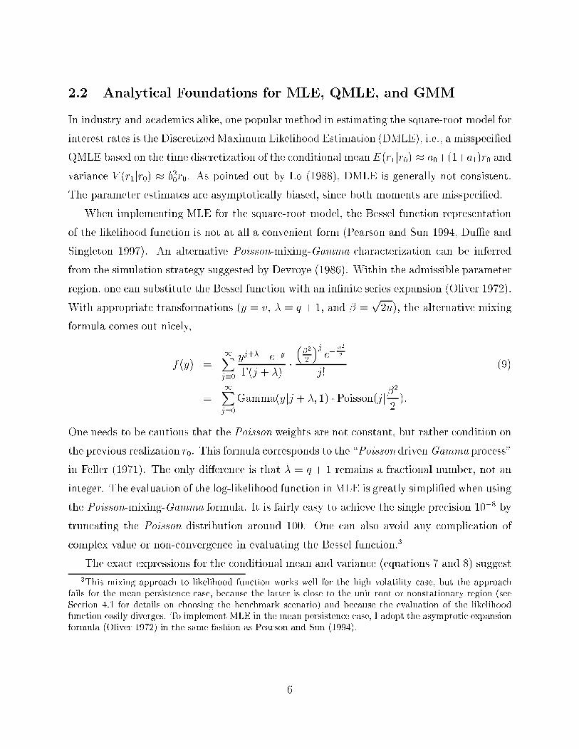
When implementing MLE for the square-root model, the Bessel function representation

of the likelihood function is not at all a convenient form (Pearson and Sun 1994, DuÆe and

Singleton 1997). An alternative Poisson-mixing-Gamma characterization can be inferred

from the simulation strategy suggested by Devroye (1986). Within the admissible parameter

region, one can substitute the Bessel function with an in�nite series expansion (Oliver 1972).

With appropriate transformations (y = v, � = q + 1, and � =p2u), the alternative mixing

formula comes out nicely,

f(y) =1Xj=0

yj+��1e�y

�(j + �)���2

2

�je�

�2

2

j!(9)

=1Xj=0

Gamma(yjj + �; 1) � Poisson(jj�2

2):

One needs to be cautious that the Poisson weights are not constant, but rather condition on

the previous realization r0. This formula corresponds to the \Poisson driven Gamma process"

in Feller (1971). The only di�erence is that � = q + 1 remains a fractional number, not an

integer. The evaluation of the log-likelihood function in MLE is greatly simpli�ed when using

the Poisson-mixing-Gamma formula. It is fairly easy to achieve the single precision 10�8 by

truncating the Poisson distribution around 100. One can also avoid any complication of

complex value or non-convergence in evaluating the Bessel function.3

The exact expressions for the conditional mean and variance (equations 7 and 8) suggest

3This mixing approach to likelihood function works well for the high volatility case, but the approachfails for the mean persistence case, because the latter is close to the unit root or nonstationary region (seeSection 4.1 for details on choosing the benchmark scenario) and because the evaluation of the likelihoodfunction easily diverges. To implement MLE in the mean persistence case, I adopt the asymptotic expansionformula (Oliver 1972) in the same fashion as Pearson and Sun (1994).

6

a quasi-maximum likelihood estimator (QMLE) for the square-root model,

maxfa0;a1;b0g

T�1Xt=1

log1q

2�V (rt+1jrt)exp

(� [rt+1 � E(rt+1jrt)]2

2V (rt+1jrt)

): (10)

QMLE is shown to be root-n consistent (Bollerslev and Wooldridge 1992) and asymptotically

normal (Newey and Steigerwald 1997) under some mild regularity conditions.

For comparison purposes, a generalized method of moments (GMM) estimator can be

constructed from the following moment vector

ft(a0; a1; b0) =

26664

rt+1 � E(rt+1jrt)rt[rt+1 � E(rt+1jrt)]

V (rt+1jrt)� [rt+1 � E(rt+1jrt)]2rtfV (rt+1jrt)� [rt+1 � E(rt+1jrt)]2g

37775 : (11)

The parameter is estimated by min g0TWgT , where gT = 1=TPT�1

t=1 ft andW is the asymptotic

variance-covariance matrix of gT (Hansen 1982). A two step estimator is adopted here.

2.3 Inference

Since we know the true parameter value for MLE, the likelihood ratio tests can determine how

often the con�dence region centered at the estimated parameter value contains the truth.

The same principle may be extended to QMLE if the expected quasi-likelihood function

is uniquely maximized at the truth (satisfying identi�cation requirement). In addition to

the correct speci�cation of the mean and variance, the remaining innovation error must be

centered at zero or have a symmetric distribution (Newey and Steigerwald 1997). QMLE

for the square-root model meets these conditions. Also, the sample-size normalized criterion

function value in GMM provides a speci�cation test distributed as a Chi-square (1).

The standard error for an individual parameter is estimated by the inverted Hessian

formula in MLE, the OPG-Hessian-OPG formula in QMLE, and the Gradient-Weighting

Matrix-Gradient formula in GMM.

2.4 Simulation

This characterization (equation 9) also de�nes a composite method to simulate the square-

root process (Devroye 1986). First, one draws a random number j from the Poisson(jj�2=2).

7

Then, one draws another random number y from the Gamma(yjj + �; 1). Finally, one

calculates the desired state variable r1 by r1 = y=c. Notice that the realized r1 is the

conditioning value r0 in the next draw. The initial value r0, when starting a simulation run,

can be set to the theoretical unconditional mean. To pass on the transient e�ect, the �rst

1000 realizations can be discarded.

3 EÆcient Method of Moments Estimation

This section describes the EMM estimator in a univariate case. For formal discussions, see

Gallant and Tauchen (1996c), Tauchen (1997), and Gallant and Long (1997).

3.1 Approximating True Density with Auxiliary Model

Denote the invariant probability measure implied by the underlying data generating process

as the p-model. It is assumed that the direct maximum likelihood estimation of the p-model

is not available. However, any smooth density function can be approximated arbitrarily close

by a Hermite polynomial expansion.

Consider a scalar case. Let y be the random variable, x be the lagged y, and � be the

parameter. The auxiliary f -model has a density function de�ned by a modi�ed Hermite

polynomial,

f(yjx; �) = Cf[P(z; x)]2�(yj�x; �2

x)g; (12)

where P is a polynomial with degree Kz in z and thus the square of P makes the density

positive. The argument of the polynomial is z, which is the transformation z = (y��x)=�x.

The coeÆcient of the polynomial is another polynomial of degree Kx in x. The constant in

the polynomial is set to 1 for identi�cation. C is a normalizing factor to make the density

proper.4 �(�) is a normal density of y with conditional mean �x and conditional variance �2x.

The length of the auxiliary model parameter is determined by the lag in mean L�, lag in

variance Lr, lag in polynomial coeÆcient Lp, polynomial degree Kz, and polynomial degree

Kx. Let f~ytgnt=1 be the observed data and ~xt�1 be the lagged observations. The sample mean

4In the case of multivariate density, the interaction terms in both the Hermite polynomial and thecoeÆcient polynomial can be set to zero, in order for a gradual expansion of the auxiliary model. See abovereferences for details.

8

log-likelihood function is de�ned by

Ln(�; f~ytgnt=1) =1

n

nXt=1

log[f(~ytj~xt�1; �)]: (13)

A quasi-maximum-likelihood estimator is obtained by

~� = argmax�Ln(�; f~ytgnt=1): (14)

The dimension of the auxiliary f -model, the length of �, is selected by Schwarz's Bayesian

Information Criterion (BIC). There are di�erent choices of information criteria for optimal

model selection. For a �nite dimensional stationary process, BIC with a larger penalty for

model complexity proves to be consistent, while the Akaike's Information Criterion (AIC)

will over�t the model. On the other hand, if the true dimension is in�nity or increases to

in�nity with the sample size, AIC with a smaller penalty for model complexity is optimal

(Zheng and Loh 1995). The dimensions of the f-model needs to be as large as the p-model

to meet the identi�cation condition.5

3.2 Matching Auxiliary Scores with Minimum Chi-Square

From the �rst-stage seminonparametric estimates, one obtains the �tted scores as the mo-

ment conditions,

mn(~�) =1

n

nXt=1

@

@�log f(~ytj~xt�1; ~�): (15)

In the second stage, a SMM-type estimator is implemented in the following way. Although

the direct MLE for p-model is assumed to be impossible, the simulation from the structural

model (e.g., the stochastic di�erential equation) is readily available. Let fytgNt=1 be a long

simulation from a candidate value of �, the parameter of the maintained structural model.

The auxiliary score functions can be reevaluated by numerical integration of of the score

functions with the simulated data,

mN (�; ~�) =1

N

NXt=1

@

@�log f(ytjxt�1; ~�); (16)

5Even when the underlying p-model has a �xed dimension (i.e., a �xed number of parameters), theauxiliary f -model can still have an increasing order in �nite sample sizes, because of the approximation fromauxiliary model to true model.

9

and the minimum chi-square estimator is simply,

� = argmin�fmN (�; ~�)

0~I�1mN(�; ~�)g; (17)

where the weighting matrix ~I�1 is estimated by the mean-outer-product of scores from the

auxiliary model

~I =1

n

nXt=1

[@

@�log f(~ytj~xt�1; ~�)][ @

@�log f(~ytj~xt�1; ~�)]0: (18)

Remember that the �nite sample eÆciency loss of the GMM-type estimators is largely

attributed to the high cost and low accuracy in estimating the serially correlated weighting

matrix. In EMM the moment conditions (score functions) of the �rst step QMLE are or-

thogonal by construction; hence the information matrix is diagonal or nearly diagonal (i.e.,

serially uncorrelated). EMM will be asymptotically as eÆcient as MLE if the following con-

ditions are met: the dimension of the auxiliary model is suÆciently large (K !1), the lag

in the the auxiliary model is suÆciently long (L !1), and the simulation from the main-

tained structural model is suÆciently long (N ! 1). This encompasses both Markovian

and non-Markovian cases (Gallant and Long 1997).

3.3 Overrejection and Misspeci�cation

The normalized criterion function value in the EMM estimation,

c2n = nmN (�; ~�)0~I�1mN (�; ~�); (19)

forms a speci�cation test for the overidentifying restrictions. Under the correct speci�cation

of the maintained model (Tauchen 1997), we have c2nD�! X 2(l� � lp), where the degree of

freedom equals the parameter length of the auxiliary model minus that of the structural

model. However, if the maintained model is misspeci�ed (Tauchen 1997), we have

c2nn

a:s:�! �c2 = mN(��; ��)0�I�1mN(��; ��) > 0;

where ��, ��, and �I are the asymptotic pseudo-true values under the maintained misspeci�-

cation. As long as the sample size n is large enough, the SNP score generator will be rich

enough such that the false passage �c2 = 0 will not occur under misspeci�cation.

10

4 Monte Carlo Design and Benchmark Choice

Technical aspects of the Monte Carlo experiment are summarized here. Most importantly,

two demanding scenarios|mean persistence and high volatility|are chosen as the bench-

marks. Also, a maintained model of interest rate with stochastic volatility and level feedback

is designated as the data generating process for comparing the power of detecting misspeci-

�cation.

4.1 Experimental Design

All computations are performed on Sun Unix Workstations|Sparc10, Sparc20, and Pentium

II-300. Programs for generating random samples and GMM, QMLE, and MLE estimations

of the square-root model are written in FORTRAN language. The FORTRAN codes for

SNP and EMM are modi�ed from SNP Version 8.5 (Gallant and Tauchen 1996b) and EMM

Version 1.3 (Gallant and Tauchen 1996a), incorporating automatic SNP search by BIC in

some of the EMM estimations. NPSOL (Gill, Murray, Saunders, and Wright 1991) is the

optimization routine used for all of the programs.

The number of Monte Carlo replications is chosen as 1000 for each scenario and each esti-

mator. Two �nite sample sizes|500 and 1500 weekly observations|are used for contrasting

the asymptotic behavior of each estimator. To generate the pseudo-random samples, the

Poisson-mixing-Gamma formula in Section 2 is implemented, and the 1000 initial stretch

is discarded each time in order to pass on the transient e�ect. The second stage of EMM

estimation is similar to SMM. The simulation size should be at least 30,000. EMM does

stabilize from 50,000 to 75,000 and could have more Monte Carlo errors at 100,000. Thus

50,000 turns out to be a conservative but economical choice (Gallant and Tauchen 1998b).

To choose a SNP score generator in the EMM estimation, one can either let BIC auto-

matically decide the SNP dimension in each replication, or, one can use a \posterior" �xed

SNP speci�cation. For the comparisons with MLE, QMLE, and GMM estimators, I use

the �xed SNP score in EMM estimation, such that the overrejection test statistics has the

same degree of freedom for each sample size. However, in order to choose an appropriate

�xed SNP score, I �rst run EMM 1000 times with the automatic SNP score generator. I

then adopt one particular score for the 500 sample size and another for the 1500 sample

11

size. These speci�cations are at relatively higher dimensions, with abundant occurrence but

without severe rejection. A by-product of the EMM estimation with automatic SNP score is

that some light can be shed on how the overrejection bias varies with the number of moments

chosen by the SNP estimation.6

In terms of the computing time, each QMLE run takes about 3-5 seconds; each GMM

run takes about 5-10 seconds; each MLE run takes about 5-10 minutes; and each EMM run

takes about 1-2 hours. Note that MLE requires numerical approximation to the likelihood

function and also that EMM uses numerical integration to evaluate the moment conditions.

EMM estimator is programmed up and ready to be implemented (Gallant and Tauchen

1996b, Gallant and Tauchen 1996a). One only needs to incorporate the square-root model

in the simulation code. The developing time for QMLE and EMM is minimal, while GMM

especially MLE requires a lot of �ne-tuning. Overall, EMM is still the most computationally

intensive method, although there are numerical techniques to speed up the estimation (e.g.,

parallel processing or antithetic simulation).

4.2 Benchmark Model

To select a suitable parameter setting, we start with the empirical result from Gallant and

Tauchen (1998b), drt = (0:02491� 0:00285rt)dt+ 0:0275r1=2t dWt. Using equations 3, 4, and

6-8, one can calculate the unconditional mean and variance, the Bessel function order, and

the conditional mean and variance. It is not diÆcult to see that this original speci�cation,

Scenario 1 in Table 1, features low mean-reversion (E(rt+1jrt) is nearly the unit-root) and

low conditional volatility (V (rt+1jrt) is close to zero). Also the unconditional variance is

unusually small, representing an abnormally quiet process. The order of the Bessel function,

twice of which corresponds to the degree of freedom for an integer order noncentral chi-square

distribution, is so large that the conditional density looks almost Gaussian. Not withstanding

all these short comings, scenario 1 is still the typical empirical result. It poses an important

challenge to researchers in �tting the highly persistent, nearly unit-root conditional mean

process, although its volatility structure and innovation density are not rich enough. Hence

6This automatic-plus-�xed SNP-EMM procedure mimics the realistic situation, when an empirical re-searcher not only relies on BIC as an objective criterion in model selection but also incorporates priorsubjective information to expand the auxiliary model|e.g, the E-GARCH score generator in Andersen et al.(1999).

12

it will only rarely generate the high order ARCH or the high degree polynomial in the SNP

score. Based on the empirical results in Gallant and Tauchen (1998b), I use the established

SNP score for Scenario 1|s14140 for the 500 sample size and s14141 for the 1500 sample

size7|and I report only the �xed score EMM estimations. The Scenario 1 in Table 1 is

termed an LMR-LCV speci�cation (low-mean-reversion and low-conditional-volatility).

If one increases only the variance parameter b0 from Scenario 1 to 2-4 in Table 1, the Bessel

function order q decreases gradually from the Gaussian-like speci�cation, but the conditional

volatility is still negligible. Alternatively, one can increase both the mean parameters a0 and

a1 by a factor of 100 and the variance parameter b0 by a factor of 10 from Scenario 1 to

5 as in Table 1, while holding the unconditional mean and variance constant. This change

will increase the conditional volatility slightly, but the Bessel function order q is still quite

large (resembling a Gaussian-like distribution). If one increases the variance parameter b0

from Scenario 5 to 6-8 as shown in Table 1, both high conditional volatility and small Bessel

function order are achieved. Scenario 8 is rich enough in both the conditional volatility

and non-Gaussian innovation, hence Scenario 8 is suitable for examining the automatic SNP

score EMM estimations. Strong volatility cluster is another challenge in �tting the short

interest rate, although the high persistence in mean is sacri�ced somewhat. Scenario 8 in

Table 1, drt = (2:491 � 0:285rt)dt + 1:1r1=2t dWt, is termed an HMR-HCV speci�cation

(high-mean-reversion and high-conditional-volatility).

One should not arbitrarily relate either Scenario 1 or Scenario 8 alone to the real interest

rate, but put together they represent the most important features in short rate process.

There is a fundamental concern with how exible the square-root model can be. In order

to �t the real interest rate data, one would like to hold the unconditional mean (�a0=a1)constant without explosion (b0 � 4a20), resembling a stationary interest rate process. In

addition one would like to achieve high persistence in both conditional mean and variance.

With only three parameters to manipulate, it seems impossible to satisfy all four constraints

simultaneously. This indicates that the square-root model may not be exible enough to

model the interest rate dynamics. To �nd a more suitable model requires a fourth degree of

7s14140 means 1 lag in mean, 4 lag in variance, 1 lag in coeÆcient polynomial, 4 degree Hermite polyno-mial, and 0 degree coeÆcient polynomial. s14141 only di�ers in 1 lag coeÆcient polynomial. There is moredetailed discussion of the SNP structure in Section 3.1.

13

freedom, for example, a stochastic volatility component (Gallant and Tauchen 1998b).

4.3 Testing Misspeci�cation

The goal is to �nd a true data generating process, of which an adequate auxiliary score will

not accommodate a misspeci�ed model. As discussed in Section 1, the square-root model

is widely used in �tting the short rate process, but most serious studies have rejected this

speci�cation. So it is natural to adopt the square-root process as a misspeci�ed model and

use a non-rejected model as the true data generating process (for the short interest rate).

A recent study by Gallant and Tauchen (1998b) gave the most favorable evidence for the

following speci�cation,

drt = (0:014� 0:002rt)dt+ (0:043� 0:018rt)eutdW1t; (20)

dut = (�0:006rt � 0:157ut)dt+ (0:593� 0:052ut)dW2t: (21)

The short rate process rt has a linear drift and a linear di�usion, with the di�usion multiplied

by an unobserved (exponential) stochastic volatility term eut. The short rate rt is only

partially observable in discrete time. The latent stochastic volatility process ut also has

a linear drift and a linear di�usion, with the drift including a short rate level feedback.

This model adequately passed the speci�cation test for various simulation sizes and greatly

outperformed the competing models in terms of reprojecting the conditional density and the

conditional volatility. It would be a very suitable choice for the true data generating process.

When we �t the misspeci�ed square-root model drt = (a0 + a1rt)dt + b0r1=2t dWt to the

interest rate data simulated from the maintained true speci�cation (equations 20 and 21),

the drift is correctly speci�ed as a linear function, and the misspeci�cation comes only into

the di�usion. From Ito's formula we know that the conditional mean is also correctly speci-

�ed as linear; therefore the drift parameters are consistent estimates (A��t-Sahalia 1996a). It

is equivalent to the case where Ordinary Least Square is consistent, but unaccounted het-

eroskedastic and/or correlated error structure may cause very noisy and ineÆcient estimates.

The misspeci�ed di�usion generates inconsistent estimates of the conditional variance, which

may cause serious distortions in pricing discount bond yields or other interest rate sensitive

derivatives. Therefore detecting the misspeci�cation in di�usion or volatility is a critical

challenge to researchers and practitioners.

14

5 Monte Carlo Results

Tables 2 through 6 and Figures 1 through 9 summarize the major �ndings of this paper. The

discussions are organized along topics, and extensive comparisons are made across QMLE,

EMM, GMM, and MLE. The main focuses are �nite sample eÆciency, overrejection bias of

EMM under the null, and the detection of maintained misspeci�cation in EMM and GMM.

Both the automatic score generator and the �xed score generator are used in EMM. The

likelihood ratio tests in MLE and QMLE provide joint inferences under the null.

5.1 Simulation Schemes

The Poisson-mixing-Gamma formula is a useful characterization of the transitional density

of the square-root model. The simulation accuracy based on the distribution function can

provide an independent check for the derivations in Section 2. The Monte Carlo study is

not alone in needing a reliable simulator; further applications of MLE with this formula

also require some justi�cation. A cornerstone of the EMM estimator|a simulation-based

estimator|is the discretized approximation to stochastic di�erential equations. EMM uses

a weak-order 2 scheme (Kloeden and Platen 1992). To assess these simulation approaches,

some empirical statistics from long realizations (100,000) are compared to their theoretical

counterparts.

Table 2 lists the calculation of two moments and three quantiles. Clearly both schemes

from exact distribution and time discretization work reasonably well. In both persistent

mean and strong volatility cases, the simulated moments and quantiles are very close to the

model implied ones. It is not surprising that the probabilistic method is slightly better than

the discretized method, although the di�erence is negligible.

5.2 Score Generator

An important feature of EMM is the endogenous moment selection by a seminonparametric

score generator (SNP), which contrasts with the ad hoc choice of moment conditions in some

less sophisticated GMM or SMM estimators. The optimal SNP search and the inexpensive

weighting matrix estimate are key to the eÆciency argument, and hopefully they also im-

prove the overrejection test. It is worthwhile to check whether the SNP score captures the

15

distribution features of di�erent dependent structures before launching the full-scale Monte

Carlo experiment. Tables 3 (500 sample size) and Table 4 (1500 sample size) report the SNP

searches for the 8 scenarios in Table 1. For each setting, the frequencies of all kinds of model

choices among 100 replications are listed. Model dimension is represented by a �ve-digit

number, which stands for, consecutively, lag in mean, lag in variance, lag in polynomial,

degree of Hermite polynomial, and degree of Hermite coeÆcient polynomial.

Scenario 1 in Tables 3 and 4 is the LMR-LCV case (low-mean-reversion, low-conditional-

volatility). Not surprisingly the Gaussian auto-regression speci�cation of 10100 dominates

other choices. This �nding is consistent with the fact that the true density is nearly Gaussian

under this parameter setting (see Table 1). Moving from Scenario 1 to 2, 3, and 4, the

conditional volatility increases gradually, since the variance parameter b0 is altered (see Table

1). The dominating choice is still Gaussian, and the chances of ARCH and/or non-Gaussian

speci�cations increase slightly. Moving toward Scenarios 5-8, both mean parameters a0 and

a1 as well as variance parameter b0 are altered (see Table 1), and ultimately one reaches

the HMR-HCV case (high-mean-reversion, high-conditional-volatility). It is clear that the

SNP search favors the nonlinear, nonparametric AR-ARCH speci�cation. This is consistent

with the low Bessel function order and high conditional variance (Table 1). Largely due to

this \distribution-dependent" or \data-dependent" score generator, the EMM estimator is

claimed to be asymptotically eÆcient and hopefully more reliable in the speci�cation test.

Also evident from Tables 3 and 4 is that larger sample sizes enable the SNP to pick

up higher model dimensions. In fact, the asymptotic eÆciency argument requires that the

number of moment conditions and the lags entering each moment increase with the sample

size (Gallant and Long 1997).

A salient question is whether the structural model can be identi�ed when the SNP search

does pick the Gaussian-AR(1) score. This corresponds to a quasi-maximum likelihood esti-

mator based on the innovation assumption

zt = (rt � �0 � �1rt�1)=�2 � N(0; 1): (22)

Since the conditional mean is correctly speci�ed, the QMLE of �0 and �1 is a consistent esti-

mator of ea1 and �a0=a1(1�ea1). It is just an Ordinary Least Square with a heteroskedastic

and serially correlated error term (A��t-Sahalia 1996a). The conditional variance is mis-

16

speci�ed as the constant �2. However, according to the theory of misspeci�ed maximum

likelihood estimation (White 1994), the estimator �2 may converge to a pseudo-true value

��2. The key argument is that the misspeci�ed asymptotic variance ��2 must be a function

of the true variance parameter b0, since both conditional variance and unconditional vari-

ance are determined by b0. These asymptotic relations, two explicit and one implicit, are

indeed the binding functions in the language of Indirect Inference (Gourierous, Monfort, and

Renault 1993). Obviously the structural parameters a0, a1, and b0 are exactly identi�ed by

the auxiliary parameters �0, �1, and �2. EMM is thus a feasible �rst-order approximation

toward the Indirect Inference (Gallant and Long 1997).

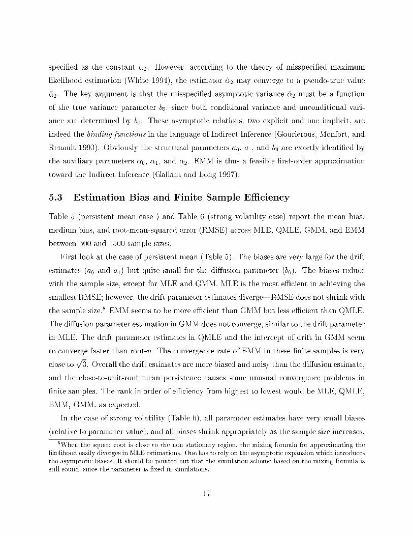
5.3 Estimation Bias and Finite Sample EÆciency

Table 5 (persistent mean case ) and Table 6 (strong volatility case) report the mean bias,

medium bias, and root-mean-squared error (RMSE) across MLE, QMLE, GMM, and EMM

between 500 and 1500 sample sizes.

First look at the case of persistent mean (Table 5). The biases are very large for the drift

estimates (a0 and a1) but quite small for the di�usion parameter (b0). The biases reduce

with the sample size, except for MLE and GMM. MLE is the most eÆcient in achieving the

smallest RMSE; however, the drift parameter estimates diverge|RMSE does not shrink with

the sample size.8 EMM seems to be more eÆcient than GMM but less eÆcient than QMLE.

The di�usion parameter estimation in GMM does not converge, similar to the drift parameter

in MLE. The drift parameter estimates in QMLE and the intercept of drift in GMM seem

to converge faster than root-n. The convergence rate of EMM in these �nite samples is very

close top3. Overall the drift estimates are more biased and noisy than the di�usion estimate,

and the close-to-unit-root mean persistence causes some unusual convergence problems in

�nite samples. The rank in order of eÆciency from highest to lowest would be MLE, QMLE,

EMM, GMM, as expected.

In the case of strong volatility (Table 6), all parameter estimates have very small biases

(relative to parameter value), and all biases shrink appropriately as the sample size increases.

8When the square-root is close to the non-stationary region, the mixing formula for approximating thelikelihood easily diverges in MLE estimations. One has to rely on the asymptotic expansion which introducesthe asymptotic biases. It should be pointed out that the simulation scheme based on the mixing formula isstill sound, since the parameter is �xed in simulations.

17

In terms of the eÆciency, the RMSE's of MLE, QMLE, and GMM are shrinking approxi-

mately at the ratep3, but the RMSE of EMM decreases faster than root-n. Recall that

EMM should be asymptotically as eÆcient as MLE, as the auxiliary SNP score generator

adopts an increasing dimension with the sample size. Overall MLE achieves the highest

eÆciency, QMLE comes second at T = 500 and third at T = 1500, EMM is third at T = 500

and second at T = 1500, GMM is best for the intercept parameter of drift but is worst for

the slope parameter of drift and the di�usion parameter. The �nding that some parameter

estimates in GMM and QMLE are slightly more eÆcient than MLE, can be attributed to the

fact that \exact" likelihood function in MLE needs to be numerically approximated while

the moment conditions in GMM or QMLE are in closed forms.

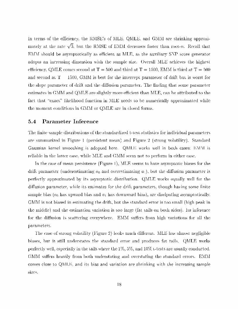
5.4 Parameter Inference

The �nite sample distributions of the standardized t-test statistics for individual parameters

are summarized in Figure 1 (persistent mean) and Figure 2 (strong volatility). Standard

Gaussian kernel smoothing is adopted here. QMLE works well in both cases; EMM is

reliable in the latter case, while MLE and GMM seem not to perform in either case.

In the case of mean persistence (Figure 1), MLE seems to have asymptotic biases for the

drift parameter (underestimating a0 and overestimating a1), but the di�usion parameter is

perfectly approximated by its asymptotic distribution. QMLE works equally well for the

di�usion parameter, while its estimates for the drift parameters, though having some �nite

sample bias (a0 has upward bias and a1 has downward bias), are dissipating asymptotically.

GMM is not biased in estimating the drift, but the standard error is too small (high peak in

the middle) and the estimation variation is too large (fat tails on both sides). Its inference

for the di�usion is scattering everywhere. EMM su�ers from high variations for all the

parameters.

The case of strong volatility (Figure 2) looks much di�erent. MLE has almost negligible

biases, but it still understates the standard error and produces fat tails. QMLE works

perfectly well, especially in the tails where the 1%, 5%, and 10% t-tests are usually conducted.

GMM su�ers heavily from both understating and overstating the standard errors. EMM

comes close to QMLE, and its bias and variation are shrinking with the increasing sample

sizes.

18

Several factors may contribute to the unusual t-test distributions: (1) high persistence

in the mean makes the simulated data look like a unit-root and the MLE, GMM, and EMM

estimators can not distinguish it from a persistent yet stationary situation in �nite samples;

(2) the so-called \exact" likelihood in MLE is approximated by its series expansion (in strong

volatility case) or its asymptotic expansion (in persistent mean case); (3) the t-test is a Wald

test and lacks invariance to nonlinear transformations.9

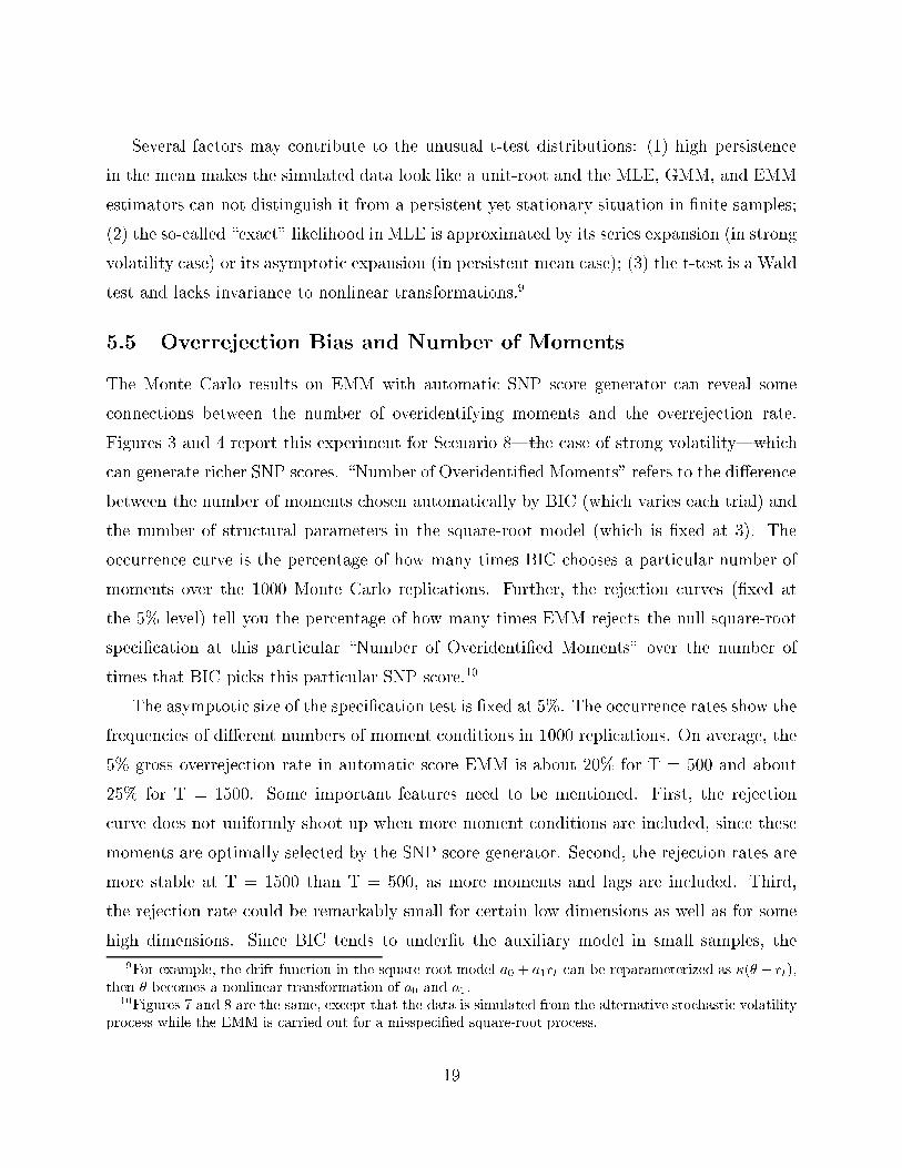
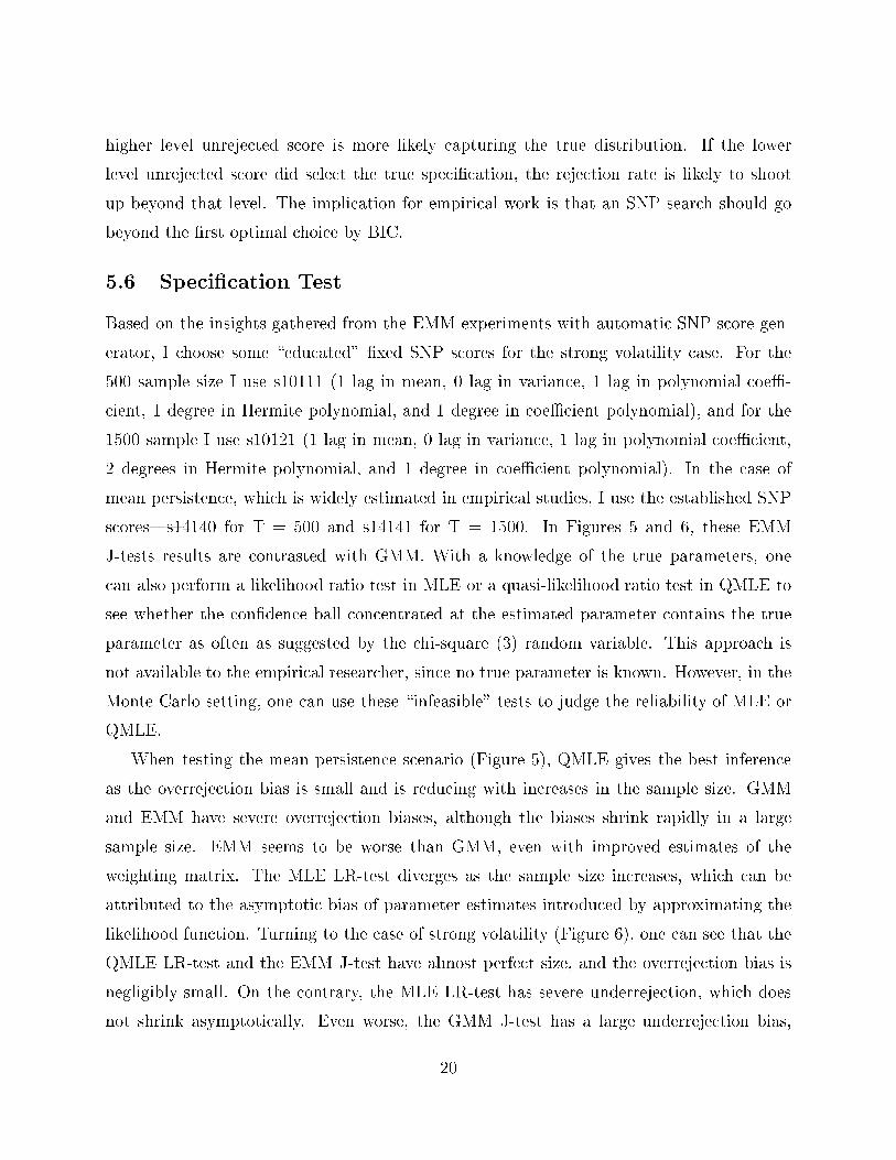
5.5 Overrejection Bias and Number of Moments

The Monte Carlo results on EMM with automatic SNP score generator can reveal some

connections between the number of overidentifying moments and the overrejection rate.

Figures 3 and 4 report this experiment for Scenario 8|the case of strong volatility|which

can generate richer SNP scores. \Number of Overidenti�ed Moments" refers to the di�erence

between the number of moments chosen automatically by BIC (which varies each trial) and

the number of structural parameters in the square-root model (which is �xed at 3). The

occurrence curve is the percentage of how many times BIC chooses a particular number of

moments over the 1000 Monte Carlo replications. Further, the rejection curves (�xed at

the 5% level) tell you the percentage of how many times EMM rejects the null square-root

speci�cation at this particular \Number of Overidenti�ed Moments" over the number of

times that BIC picks this particular SNP score.10

The asymptotic size of the speci�cation test is �xed at 5%. The occurrence rates show the

frequencies of di�erent numbers of moment conditions in 1000 replications. On average, the

5% gross overrejection rate in automatic score EMM is about 20% for T = 500 and about

25% for T = 1500. Some important features need to be mentioned. First, the rejection

curve does not uniformly shoot up when more moment conditions are included, since these

moments are optimally selected by the SNP score generator. Second, the rejection rates are

more stable at T = 1500 than T = 500, as more moments and lags are included. Third,

the rejection rate could be remarkably small for certain low dimensions as well as for some

high dimensions. Since BIC tends to under�t the auxiliary model in small samples, the

9For example, the drift function in the square-root model a0 + a1rt can be reparameterized as �(� � rt),then � becomes a nonlinear transformation of a0 and a1.

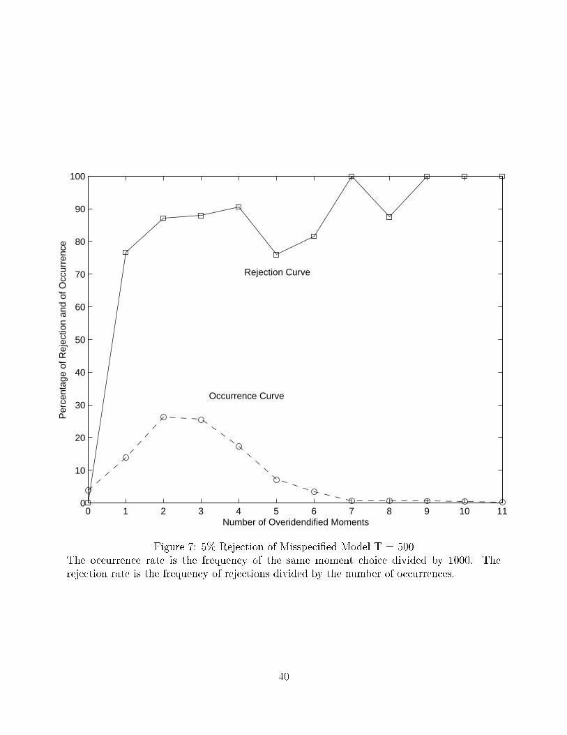
10Figures 7 and 8 are the same, except that the data is simulated from the alternative stochastic volatilityprocess while the EMM is carried out for a misspeci�ed square-root process.

19

higher level unrejected score is more likely capturing the true distribution. If the lower

level unrejected score did select the true speci�cation, the rejection rate is likely to shoot

up beyond that level. The implication for empirical work is that an SNP search should go

beyond the �rst optimal choice by BIC.

5.6 Speci�cation Test

Based on the insights gathered from the EMM experiments with automatic SNP score gen-

erator, I choose some \educated" �xed SNP scores for the strong volatility case. For the

500 sample size I use s10111 (1 lag in mean, 0 lag in variance, 1 lag in polynomial coeÆ-

cient, 1 degree in Hermite polynomial, and 1 degree in coeÆcient polynomial), and for the

1500 sample I use s10121 (1 lag in mean, 0 lag in variance, 1 lag in polynomial coeÆcient,

2 degrees in Hermite polynomial, and 1 degree in coeÆcient polynomial). In the case of

mean persistence, which is widely estimated in empirical studies, I use the established SNP

scores|s14140 for T = 500 and s14141 for T = 1500. In Figures 5 and 6, these EMM

J-tests results are contrasted with GMM. With a knowledge of the true parameters, one

can also perform a likelihood ratio test in MLE or a quasi-likelihood ratio test in QMLE to

see whether the con�dence ball concentrated at the estimated parameter contains the true

parameter as often as suggested by the chi-square (3) random variable. This approach is

not available to the empirical researcher, since no true parameter is known. However, in the

Monte Carlo setting, one can use these \infeasible" tests to judge the reliability of MLE or

QMLE.

When testing the mean persistence scenario (Figure 5), QMLE gives the best inference

as the overrejection bias is small and is reducing with increases in the sample size. GMM

and EMM have severe overrejection biases, although the biases shrink rapidly in a large

sample size. EMM seems to be worse than GMM, even with improved estimates of the

weighting matrix. The MLE LR-test diverges as the sample size increases, which can be

attributed to the asymptotic bias of parameter estimates introduced by approximating the

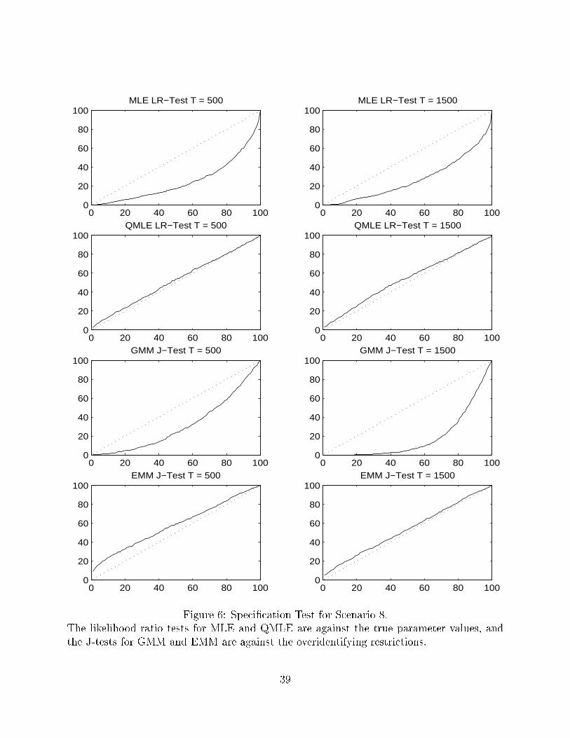
likelihood function. Turning to the case of strong volatility (Figure 6), one can see that the

QMLE LR-test and the EMM J-test have almost perfect size, and the overrejection bias is

negligibly small. On the contrary, the MLE LR-test has severe underrejection, which does

not shrink asymptotically. Even worse, the GMM J-test has a large underrejection bias,

20

which is diverging with increases in sample sizes.

There are at least four sources of overrejection or underrejection bias in GMM-type

estimators: inaccurate and costly estimates of the weighting matrix; unseasoned selection

of the moment conditions; an inadequate number of moments to capture the distribution

feature; and simply a small sample bias. A generic EMM approach overcomes the �rst two

problems by adopting a serially uncorrelated information matrix and an optimal SNP score

generator. The conservative BIC procedure in EMM may choose too few moments, but

one can rectify this problem by using additional information and extending the SNP search

beyond the BIC choice. The remaining small sample bias can be remedied by enlarging the

sample size. The above arguments carry through here, except in the case of persistent mean,

where the EMM estimator may mistake the data as coming from a unit-root process.

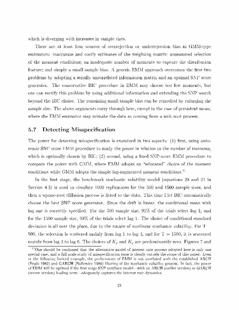
5.7 Detecting Misspeci�cation

The power for detecting misspeci�cation is examined in two aspects: (1) �rst, using auto-

matic SNP score EMM procedure to study the power in relation to the number of moments,

which is optimally chosen by BIC; (2) second, using a �xed SNP-score EMM procedure to

compare the power with GMM, where EMM adopts an \educated" choice of the moment

conditions while GMM adopts the simple lag-augmented moment conditions.11

In the �rst stage, the benchmark stochastic volatility model (equations 20 and 21 in

Section 4.3) is used to simulate 1000 replications for the 500 and 1500 sample sizes, and

then a square-root di�usion process is �tted to the data. This time I let BIC automatically

choose the best SNP score generator. Since the drift is linear, the conditional mean with

lag one is correctly speci�ed. For the 500 sample size, 91% of the trials select lag 1; and

for the 1500 sample size, 93% of the trials select lag 1. The choice of conditional standard

deviation is all over the place, due to the nature of nonlinear stochastic volatility. For T =

500, the selection is scattered mainly from lag 1 to lag 4, and for T = 1500, it is scattered

mainly from lag 3 to lag 6. The choices of Kz and Kx are predominantly zero. Figures 7 and

11One should be cautioned that the alternative model of interest rate process adopted here is only onespecial case, and a full scale study of misspeci�cation issue is clearly outside the scope of this paper. Evenin the following limited example, the performance of EMM is not unrelated with the established ARCH(Engle 1982) and GARCH (Bollerslev 1986) �ltering of the stochastic volatility process. In fact, the powerof EMM will be optimal if the �rst stage SNP auxiliary model|with an ARCH (earlier version) or GARCH(recent version) leading term|adequately captures the interest rate dynamics.

21

8 plot the 5% rejection rates against the number of overidenti�ed moments along with the

occurrence rates of these moment choices. The highlight is that the probability of rejecting

a misspeci�ed model does converge to one very quickly. At T = 500, the 5% level rejection

rate is around 80-90% for a range of overidenti�ed moments between 1 to 6, and beyond

that the rejection rate is almost 100% (Figure 7). At T = 1500, the rejection rate is always

close to 100%, except in an exactly identi�ed case (Figure 8).

In the second stage, similar to the study of the overrejection issue, I �x the SNP score

generator and look at the rejection rate uniformly along the 1%-100% test level. The �xed

SNP score generator for the 500 sample size is s13100 (1 lag in mean and 3 lags in variance),

and the chi-square test has a degree of freedom that is 3. When T = 1500, the score is

�xed at s15100 (1 lag in mean and 5 lags in variance), with 5 degrees of freedom. Figure 9

gives the rejection plot for the EMM J-test statistics, in comparison with GMM which has 1

overidenti�ed moment. The upshot is that the EMM has the power to detect a misspeci�ed

model, and the power quickly converges to one as the sample size increases from 500 to 1500.

In contrast, the GMM has a serious underrejection problem for the maintained misspeci�ca-

tion, and the underrejection bias becomes larger as sample size increases|ultimately loosing

the power to detect misspeci�cation. The explanation is quite simple: EMM chooses care-

fully a SNP moment generator by BIC, while standard GMM simply uses the lag-augmented

instruments.

6 Conclusions

This paper performs a Monte Carlo study on EÆcient Method of Moments (EMM), Gener-

alized Method of Moments (GMM), Quasi-Maximum Likelihood Estimation (QMLE), and

Maximum Likelihood Estimation (MLE) for a continuous-time square-root model under two

challenging scenarios|high persistence in mean and strong conditional volatility|that are

commonly encountered when estimating the empirical interest rate process.

MLE achieves the highest eÆciency, while its inferences on individual parameters and

overall speci�cation are not very reliable and are even misleading on some occasions. QMLE

is less eÆcient in comparison to MLE, but QMLE stands out as the best inference tool in

both the individual t-test and overall LR-test. EMM shows a convergence rate faster than

22

root-n, due to the expanding SNP score choice by BIC as sample size increases. EMM also

provides better inference than GMM or MLE in a high volatility scenario. In the case of

persistent mean|close to unit root in small samples|some asymptotics of MLE and GMM

break down, as parameter estimates and test statistics diverge.

A number of lessons can be learned from this study: (1) MLE is not necessarily the best

choice if the numerical approximation to the density is complex and/or the approximation

tends to diverges near the non-stationary region; (2) QMLE is simple to implement and can

be very reliable when the speci�cation information is easily incorporated in the closed-form

conditional mean and variance; (3) if there is no new information to be incorporated into

the moment conditions, GMM can not be superior to QMLE; (4) when the true density or

moment functions are not known, EMM is the only choice; its small sample performance is

not necessarily inferior to the infeasible MLE or QMLE and is most likely superior to the

infeasible GMM.

23

References

A��t-Sahalia, Yacine (1996a), \Nonparametric Pricing of Interest Rate Derivatives," Econo-

metrica, vol. 64, 527{560.

A��t-Sahalia, Yacine (1996b), \Testing Continuous-Time Models of the Spot Interest Rate,"

The Review of Financial Studies, vol. 9, 385{426.

Andersen, Torben G., Hyung-Jin Chung, and Bent E. S�renson (1999), \EÆcient Method of

Moments Estimation of a Stochastic Volatility Model: A Monte Carlo Study," Journal

of Econometrics, vol. 91, 61{87.

Andersen, Torben G. and Bent E. S�renson (1996), \GMMEstimation of a Stochastic Volatil-

ity Model: A Monte Carlo Study," Journal of Business and Economic Statistics, vol. 14,

328{352.

Bansal, Ravi, A. Ronald Gallant, Robert Hussey, and George Tauchen (1995), \Nonpara-

metric Estimation of Structural Models for High-Frequency Currency Market Data,"

Journal of Econometrics, vol. 66, 251{287.

Bollerslev, Tim (1986), \Generalized Autoregressive Conditional Heteroscedasticity," Jour-

nal of Econometrics, vol. 31, 307{327.

Bollerslev, Tim and Je�ery Wooldridge (1992), \Quasi-Maximum Likelihood Estimators and

Inference in Dynamic Models with Time-Varying Covariances," Econometric Review ,

vol. 11, 143{172.

Burnside, Craig and Martin Eichenbaum (1996), \Small-Sample Properties of GMM-Based

Wald Tests," Journal of Business and Economic Statistics, vol. 14, 294{308.

Chumacero, R�omulo A. (1997), \Finite Sample Properties of the EÆcient Method of Mo-

ments," Studies in Nonlinear Dynamics and Econometrics, vol. 2, 35{51.

Conley, Tim, Lars Peter Hansen, Erzo Luttmer, and Jose Scheinkman (1997), \Short Term

Interest Rates as Subordinated Di�usions," Review of Financial Studies, vol. 10, 525{

578.

24

Cox, John C., Jonathan E. Ingersoll, and Stephen A. Ross (1985), \A Theory of the Term

Structure of Interest Rates," Econometrica, vol. 53, 385{407.

Dai, Qiang and Kenneth J. Singleton (2000), \Speci�cation Analysis of AÆne Term Structure

Models," Journal of Finance, forthcoming.

Devroye, Luc (1986), Non-Uniform Random Variate Generation, Spinger-Verlag.

DuÆe, Darrell and Kenneth Singleton (1993), \Simulated Moments Estimation of Markov

Models of Asset Prices," Econometrica, vol. 61, 929{952.

DuÆe, Darrell and Kenneth Singleton (1997), \An Econometric Model of the Term Structure

of Interest-Rate Swap Yields," Journal of Finance, vol. 52, 1287{1321.

Engle, Robert F. (1982), \Autoregressive Conditional Heteroscedasticity with Estimates of

the Variance of U.K. In ation," Econometrica, vol. 50, 987{1008.

Feller, Wiliam (1951), \Two Singular Di�usion Problems," Annals of Mathematics, vol. 54,

173{182.

Feller, Wiliam (1971), An Introduction to Probability Theory and Its Applications, vol. 2,

John Wiley & Sons, Inc., Princeton University, 2nd ed.

Fisher, Mark and Christian Gilles (1996), \Estimating Exponential AÆne Models of the

Term Structure," Working Paper .

Gallant, A. Ronald and Jonathan R. Long (1997), \Estimating Stochastic Di�erential Equa-

tions EÆciently by Minimum Chi-Square," Biometrika, vol. 84.

Gallant, A. Ronald and George Tauchen (1996a), User's Guide for EMM: A Program for

EÆcient Method of Moments Estimation, 1st ed.

Gallant, A. Ronald and George Tauchen (1996b), User's Guide for SNP: A Program for

Nonparametric Time Series Analysis, 8th ed.

Gallant, A. Ronald and George Tauchen (1996c), \Which Moment to Match?" Econometric

Theory , vol. 12, 657{681.

25

Gallant, A. Ronald and George Tauchen (1998a), \The Relative EÆciency of Method of

Moments Estimators," Working Paper .

Gallant, A. Ronald and George Tauchen (1998b), \Reprojecting Partially Observed Sys-

tems with Application to Interest Rate Di�usions," Journal of the American Statistical

Association, vol. 93, 10{24.

Gibbons, Michael R. and Krishna Ramaswamy (1993), \A Test of the Cox, Ingersoll, and

Ross Model of the Term Structure," Review of Financial Studies, vol. 6, 619{658.

Gill, Philip E., Walter Murray, Michael A. Saunders, and Margaret H. Wright (1991), \User's

Guide for NPSOL (Version 4.06): A Fortran Package for Nonlinear Programming,"

Tech. rep., Stanford University.

Gourierous, C., A. Monfort, and E. Renault (1993), \Indirect Inference," Journal of Applied

Econometrics, vol. 8, s85{s118.

Hansen, Lars Peter (1982), \Large Sample Properties of Generalized Method of Moments

Estimators," Econometrica, vol. 50, 1029{1054.

Hansen, Lars Peter, John Heaton, and Amir Yaron (1996), \Finite-Sample Properties of

Some Alternative GMM Estimators," Journal of Business and Economic Statistics,

vol. 14, 262{280.

Hansen, Lars Peter and Jose Alexandre Scheinkman (1995), \Back to the Future: Gen-

eralized Moment Implications for Continuous Time Markov Process," Econometrica,

vol. 63, 767{804.

Ingram, Beth F. and B. S. Lee (1991), \Simulation Estimation of Time Series Models,"

Journal of Econometrics, vol. 47, 197{205.

Johnson, Norman L. and Samuel Kotz (1970), Distributions in Statistics: Continuous Uni-

variate Distributions, vol. 2, John Wiley & Sons.

Karatzas, Ioannis and Steven E. Shreve (1997), Brownian Motion and Stochastic Calculus,

Springer.

26

Kloeden, Peter E. and Eckhard Platen (1992), Numerical Solution of Stochastic Di�erential

Equations, Applications of Mathematics, Springer-Verlag.

Lo, Andrew W. (1988), \Maximum Likelihood Estimation of Generalized It'o Process with

Discretely Sampled Data," Econometric Theory , vol. 4, 231{247.

Newey, Whitney K. and Douglas G. Steigerwald (1997), \Asymptotic Bias for Quasi-

Maximum-Likelihood Estimators in Conditional Heteroscedasticity Models," Economet-

rica, vol. 65, 587{599.

Oliver, F. W. J. (1972), Handbook of Mathematical Functions with Formulas, Graphs, and

Mathematical Tables, John Wiley & Sons.

Pearson, Neil D. and Tong-Sheng Sun (1994), \Exploiting the Conditional Density in Esti-

mating the Term Structure: An Application to the Cox, Ingersoll, and Ross Model,"

Journal of Finance, vol. 49, 1279{1304.

Tauchen, George (1997), \New Minimum Chi-Square Methods in Empirical Finance," in

\Advances in Econometrics, Seventh World Congress," (edited by Kreps, D. and K. Wal-

lis), Cambridge University Press, Cambridge UK.

White, Halbert (1994), Estimation, Inference, and Speci�cation Analysis, Cambridge Uni-

versity Press, University of California, San Diego.

Zheng, Xiaodong and Wei-Yin Loh (1995), \Consistent Variable Selection in Linear Models,"

Journal of the American Statistical Association, vol. 90, 1029{1054.

27

Table 1: Benchmark Model ChoiceThe square-root model is drt = (a0 + a1rt)dt + b0r

1=2t dWt. Scenario 1 is taken from Gallant

and Tauchen (1998b). In Scenarios 2-4, the variance parameter b0 is increased by a factorof 2, 3, and 4 respectively. From Scenario 1 to Scenario 5, the mean parameters a0 and a1are multiplied by 100 and the variance parameter b0 is multiplied by 10. From Scenario 5 toScenarios 6-8, the variance parameter b0 is increased by a factor of 2, 3, and 4 respectively.E(rt), V (rt), q, E(rt+1jrt), and V (rt+1jrt) are calculated using equations 3, 4, and 6-8.

Scenario 1 Scenario 2 Scenario 3 Scenario 4a0 = 0:02491 a0 = 0:02491 a0 = 0:02491 a0 = 0:02491

a1 = �0:00285 a1 = �0:00285 a1 = �0:00285 a1 = �0:00285b0 = 0:0275 b0 = 0:055 b0 = 0:0825 b0 = 0:11

E(rt) 8.74 8.74 8.74 8.74V (rt) 1.16 4.64 10.44 18.55Bessel q 64.88 15.47 6.32 3.12E(rt+1jrt) 0.997rt+0.025 0.997rt+0.025 0.997rt+0.025 0.997rt+0.025V (rt+1jrt) 0.001rt+0.000 0.003rt+0.000 0.007rt+0.000 0.012rt+0.000

Scenario 5 Scenario 6 Scenario 7 Scenario 8a0 = 2:491 a0 = 2:491 a0 = 2:491 a0 = 2:491

a1 = �0:285 a1 = �0:285 a1 = �0:285 a1 = �0:285b0 = 0:275 b0 = 0:55 b0 = 0:825 b0 = 1:1

E(rt) 8.74 8.74 8.74 8.74V (rt) 1.16 4.64 10.44 18.55Bessel q 64.88 15.47 6.32 3.12E(rt+1jrt) 0.75rt+2.17 0.75rt+2.17 0.75rt+2.17 0.75rt+2.17V (rt+1jrt) 0.05rt+0.07 0.20rt+0.29 0.45rt+0.64 0.79rt+1.14

28

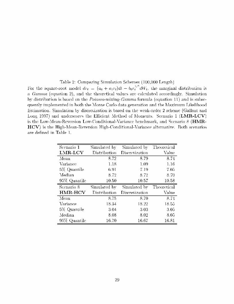
Table 2: Comparing Simulation Schemes (100,000 Length)

For the square-root model drt = (a0 + a1rt)dt + b0r1=2t dWt, the marginal distribution is

a Gamma (equation 2), and the theoretical values are calculated accordingly. Simulationby distribution is based on the Poisson-mixing-Gamma formula (equation 11) and is subse-quently implemented in both the Monte Carlo data generation and the Maximum LikelihoodEstimation. Simulation by discretization is based on the weak-order 2 scheme (Gallant andLong 1997) and underscores the EÆcient Method of Moments. Scenario 1 (LMR-LCV)is the Low-Mean-Reversion Low-Conditional-Variance benchmark, and Scenario 8 (HMR-

HCV) is the High-Mean-Reversion High-Conditional-Variance alternative. Both scenariosare de�ned in Table 1.

Scenario 1 Simulated by Simulated by TheoreticalLMR-LCV Distribution Discretization ValueMean 8.72 8.79 8.74Variance 1.18 1.09 1.165% Quantile 6.91 7.19 7.05Median 8.72 8.72 8.7095% Quantile 10.50 10.57 10.58

Scenario 8 Simulated by Simulated by TheoreticalHMR-HCV Distribution Discretization ValueMean 8.75 8.70 8.74Variance 18.34 18.22 18.555% Quantile 3.04 3.03 3.05Median 8.08 8.02 8.0595% Quantile 16.70 16.67 16.81

29

Table 3: SNP Search for the Sample Size of 500(This note applies to both Table 3 and Table 4.) These results are from 100 replicationsof each scenario with the sample sizes of 500 and 1500. The information criterion used inmoment selection is Schwarz's BIC. Scenarios 1-8 are the same as those in Table 1. Eachmodel speci�cation is characterized by a 5-digit number. Each digit consecutively stands forlag in mean, lag in variance, lag in polynomial, degree of Hermite polynomial, and degree ofHermite coeÆcient polynomial.

Scenario 1 Scenario 2 Scenario 3 Scenario 4Model % Model % Model % Model %10100 95 10100 96 10100 92 10100 8811100 3 20100 3 10110 4 11100 720100 1 10110 1 11100 2 10110 121100 1 20100 2 10120 1

20100 121100 111111 1

Scenario 5 Scenario 6 Scenario 7 Scenario 8Model % Model % Model % Model %10100 90 10100 77 10100 46 10111 2510110 5 10110 12 10110 25 10100 1820100 3 11110 4 10111 8 10110 1511100 1 11100 3 10121 7 10121 1110120 1 10111 1 10120 6 11110 10

10120 1 11110 3 11120 612110 1 10130 1 10120 420100 1 11100 1 12120 3

11120 1 10131 211130 1 11130 212110 1 10112 1

11111 115110 121120 1

30

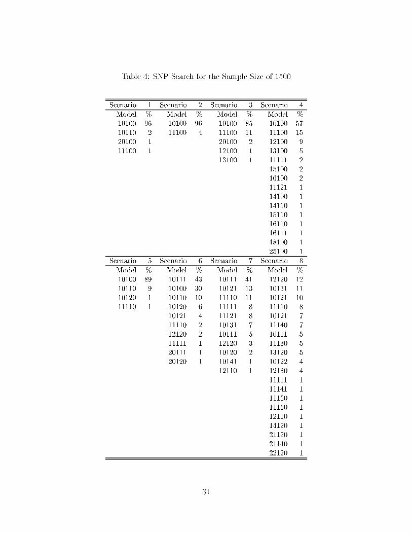
Table 4: SNP Search for the Sample Size of 1500

Scenario 1 Scenario 2 Scenario 3 Scenario 4

Model % Model % Model % Model %

10100 96 10100 96 10100 85 10100 57

10110 2 11100 4 11100 11 11100 15

20100 1 20100 2 12100 9

11100 1 12100 1 13100 5

13100 1 11111 2

15100 2

16100 2

11121 1

14100 1

14110 1

15110 1

16110 1

16111 1

18100 1

25100 1

Scenario 5 Scenario 6 Scenario 7 Scenario 8

Model % Model % Model % Model %

10100 89 10111 43 10111 41 12120 12

10110 9 10100 30 10121 13 10131 11

10120 1 10110 10 11110 11 10121 10

11110 1 10120 6 11111 8 11110 8

10121 4 11121 8 10121 7

11110 2 10131 7 11140 7

12120 2 10111 5 10111 5

11111 1 12120 3 11130 5

20111 1 10120 2 13120 5

20120 1 10141 1 10122 4

12110 1 12130 4

11111 1

11141 1

11150 1

11160 1

12110 1

14120 1

21120 1

21140 1

22120 1

31

Table 5: Finite Sample Bias and EÆciency Comparison for Scenario 1For each sample size, 1000 Monte Carlo replications are generated from the square-root pro-cess, and the model is estimated by MLE, QMLE, GMM, and EMM respectively. Scenario 1is the Low-Mean-Reversion Low-Conditional-Variance (LMR-LCV) case. EMM estimationin this table uses a �xed SNP score generator.

Mean Bias Median Bias RMSETrue Value T = 500 T = 1500 T = 500 T = 1500 T = 500 T = 1500

Maximum Likelihood Estimationa0= 0.02491 -0.0123 -0.0130 -0.0119 -0.0126 0.0125 0.0131a1=-0.00285 0.0014 0.0015 0.0014 0.0014 0.0014 0.0015b0= 0.02750 -4.4e-5 2.5e-6 -4.6e-5 2.1e-5 0.0009 0.0005

Quasi-Maximum Likelihood Estimationa0= 0.02491 0.0994 0.0285 0.0803 0.0209 0.1343 0.0437a1=-0.00285 -0.0113 -0.0033 -0.0091 -0.0025 0.0153 0.0050b0= 0.02750 3.0e-5 1.2e-5 4.1e-5 1.9e-5 0.0009 0.0005

Generalized Method of Momentsa0= 0.02491 0.0019 0.0023 4.7e-5 -5.1e-7 0.2418 0.0960a1=-0.00285 -0.0012 0.0022 -7.9e-5 -5.8e-5 0.0539 0.0481b0= 0.02750 0.0040 0.0075 -7.3e-6 6.1e-6 0.1256 0.1264

EÆcient Method of Momentsa0= 0.02491 0.0451 0.0407 2.6e-4 0.0085 0.1252 0.0944a1=-0.00285 -0.0054 -0.0048 -8.1e-5 -0.0012 0.0149 0.0112b0= 0.02750 -0.0015 -0.0003 -4.8e-6 -4.3e-7 0.0076 0.0041

32

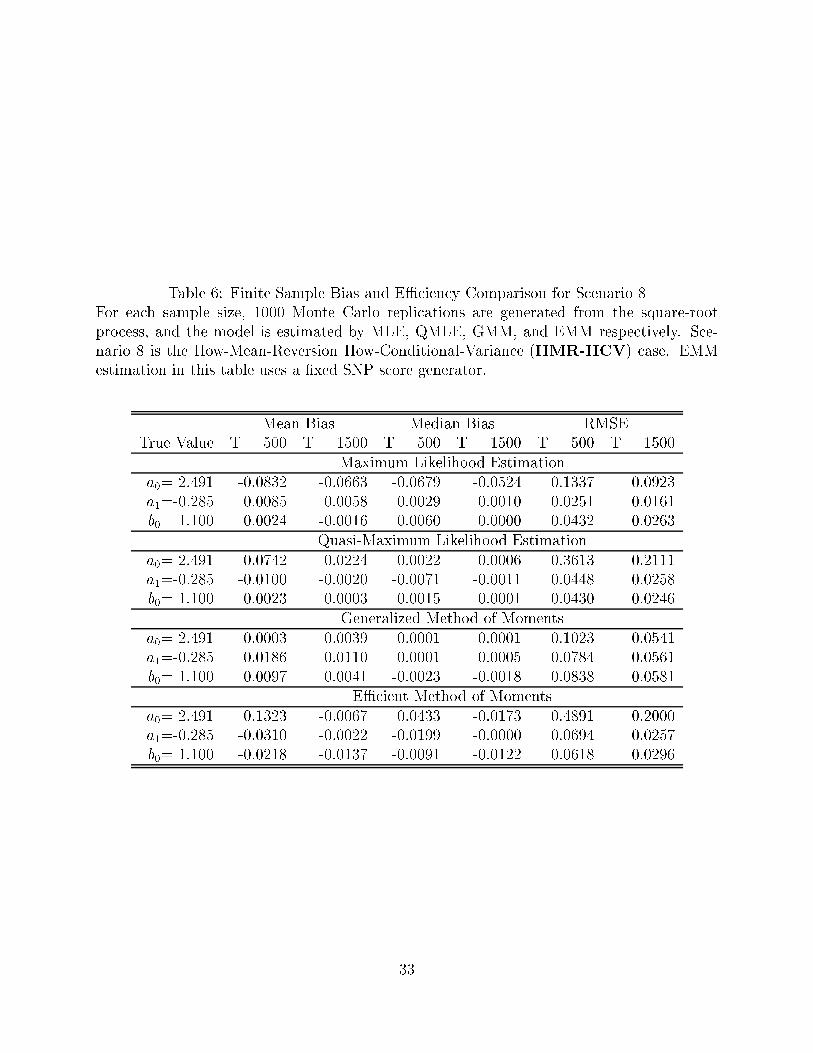
Table 6: Finite Sample Bias and EÆciency Comparison for Scenario 8For each sample size, 1000 Monte Carlo replications are generated from the square-rootprocess, and the model is estimated by MLE, QMLE, GMM, and EMM respectively. Sce-nario 8 is the How-Mean-Reversion How-Conditional-Variance (HMR-HCV) case. EMMestimation in this table uses a �xed SNP score generator.

Mean Bias Median Bias RMSETrue Value T = 500 T = 1500 T = 500 T = 1500 T = 500 T = 1500

Maximum Likelihood Estimationa0= 2.491 -0.0832 -0.0663 -0.0679 -0.0524 0.1337 0.0923a1=-0.285 0.0085 0.0058 0.0029 0.0010 0.0251 0.0161b0= 1.100 0.0024 -0.0016 0.0060 0.0000 0.0432 0.0263

Quasi-Maximum Likelihood Estimationa0= 2.491 0.0742 0.0224 0.0022 0.0006 0.3613 0.2111a1=-0.285 -0.0100 -0.0020 -0.0071 -0.0011 0.0448 0.0258b0= 1.100 0.0023 0.0003 0.0015 -0.0001 0.0430 0.0246

Generalized Method of Momentsa0= 2.491 0.0003 0.0039 0.0001 0.0001 0.1023 0.0541a1=-0.285 0.0186 0.0110 0.0001 0.0005 0.0784 0.0561b0= 1.100 0.0097 0.0041 -0.0023 -0.0018 0.0838 0.0581

EÆcient Method of Momentsa0= 2.491 0.1323 -0.0067 0.0433 -0.0173 0.4891 0.2000a1=-0.285 -0.0310 -0.0022 -0.0199 -0.0000 0.0694 0.0257b0= 1.100 -0.0218 -0.0137 -0.0091 -0.0122 0.0618 0.0296

33

−5 0 50

0.1

0.2

0.3

0.4

0.5

MLE: a0

−5 0 50

0.1

0.2

0.3

0.4

0.5

MLE: a1

−5 0 50

0.1

0.2

0.3

0.4

0.5

MLE: b0

−5 0 50

0.1

0.2

0.3

0.4

0.5

QMLE: a0

−5 0 50

0.1

0.2

0.3

0.4

0.5

QMLE: a1

−5 0 50

0.1

0.2

0.3

0.4

0.5

QMLE: b0

−5 0 50

0.1

0.2

0.3

0.4

0.5

GMM: a0

−5 0 50

0.1

0.2

0.3

0.4

0.5

GMM: a1

−5 0 50

0.1

0.2

0.3

0.4

0.5

GMM: b0

−5 0 50

0.1

0.2

0.3

0.4

0.5

EMM: a0

−5 0 50

0.1

0.2

0.3

0.4

0.5

EMM: a1

−5 0 50

0.1

0.2

0.3

0.4

0.5

EMM: b0

Figure 1: Sampling Distributions of t-Statistics for Scenario 1.The notations are respectively: \- - -" t-test statistics for 500 sample size; \|{" t-teststatistics for 1500 sample size; \-.-.-" Normal (0,1) density as the reference.

34

−5 0 50

0.1

0.2

0.3

0.4

0.5

MLE: a0

−5 0 50

0.1

0.2

0.3

0.4

0.5

MLE: a1

−5 0 50

0.1

0.2

0.3

0.4

0.5

MLE: b0

−5 0 50

0.1

0.2

0.3

0.4

0.5

QMLE: a0

−5 0 50

0.1

0.2

0.3

0.4

0.5

QMLE: a1

−5 0 50

0.1

0.2

0.3

0.4

0.5

QMLE: b0

−5 0 50

0.1

0.2

0.3

0.4

0.5

GMM: a0

−5 0 50

0.1

0.2

0.3

0.4

0.5

GMM: a1

−5 0 50

0.1

0.2

0.3

0.4

0.5

GMM: b0

−5 0 50

0.1

0.2

0.3

0.4

0.5

EMM: a0

−5 0 50

0.1

0.2

0.3

0.4

0.5

EMM: a1

−5 0 50

0.1

0.2

0.3

0.4

0.5

EMM: b0

Figure 2: Sampling Distributions of t-Statistics for Scenario 8.The notations are respectively: \- - -" t-test statistics for 500 sample size; \|{" t-teststatistics for 1500 sample size; \-.-.-" Normal (0,1) density as the reference.

35

0 2 4 6 8 10 120

10

20

30

40

50

60

70

80

90

100

Number of Overidendified Moments

Per

cent

age

of R

ejec

tion

and

of O

ccur

renc

e

Rejection Curve

Occurrence Curve

Figure 3: 5% Overrejection Rate of EMM T = 500 with Automatic Score Generator.The occurrence rate is the frequency of the same moment choice divided by 1000. Therejection rate is the frequency of rejections divided by the number of occurrences.

36

0 2 4 6 8 10 120

10

20

30

40

50

60

70

80

90

100

Number of Overidendified Moments

Per

cent

age

of R

ejec

tion

and

of O

ccur

renc

e

Rejection Curve

Occurrence Curve

Figure 4: 5% Overrejection Rate of EMM T = 1500 with Automatic Score Generator.The occurrence rate is the frequency of the same moment choice divided by 1000. Therejection rate is the frequency of rejections divided by the number of occurrences.

37

0 20 40 60 80 1000

20

40

60

80

100QMLE LR−Test T = 500

0 20 40 60 80 1000

20

40

60

80

100QMLE LR−Test T = 1500

0 20 40 60 80 1000

20

40

60

80

100MLE LR−Test T = 500

0 20 40 60 80 1000

20

40

60

80

100MLE LR−Test T = 1500

0 20 40 60 80 1000

20

40

60

80

100GMM J−Test T = 500

0 20 40 60 80 1000

20

40

60

80

100GMM J−Test T = 1500

0 20 40 60 80 1000

20

40

60

80

100EMM J−Test T = 500

0 20 40 60 80 1000

20

40

60

80

100EMM J−Test T = 1500

Figure 5: Speci�cation Test for Scenario 1.The likelihood ratio tests for MLE and QMLE are against the true parameter values, andthe J-tests for GMM and EMM are against the overidentifying restrictions.

38

0 20 40 60 80 1000

20

40

60

80

100MLE LR−Test T = 500

0 20 40 60 80 1000

20

40

60

80

100MLE LR−Test T = 1500

0 20 40 60 80 1000

20

40

60

80

100QMLE LR−Test T = 500

0 20 40 60 80 1000

20

40

60

80

100QMLE LR−Test T = 1500

0 20 40 60 80 1000

20

40

60

80

100GMM J−Test T = 500

0 20 40 60 80 1000

20

40

60

80

100GMM J−Test T = 1500

0 20 40 60 80 1000

20

40

60

80

100EMM J−Test T = 500

0 20 40 60 80 1000

20

40

60

80

100EMM J−Test T = 1500

Figure 6: Speci�cation Test for Scenario 8.The likelihood ratio tests for MLE and QMLE are against the true parameter values, andthe J-tests for GMM and EMM are against the overidentifying restrictions.

39

0 1 2 3 4 5 6 7 8 9 10 110

10

20

30

40

50

60

70

80

90

100

Number of Overidendified Moments

Per

cent

age

of R

ejec

tion

and

of O

ccur

renc

e

Rejection Curve

Occurrence Curve

Figure 7: 5% Rejection of Misspeci�ed Model T = 500The occurrence rate is the frequency of the same moment choice divided by 1000. Therejection rate is the frequency of rejections divided by the number of occurrences.

40

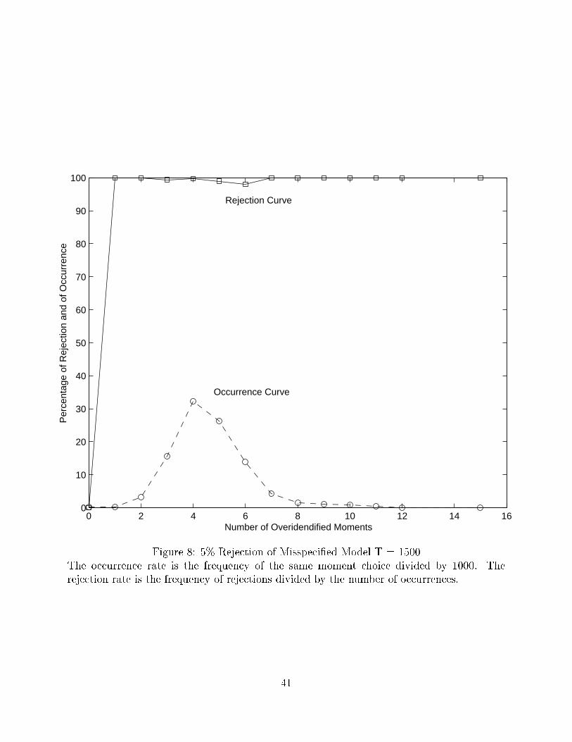
0 2 4 6 8 10 12 14 160

10

20

30

40

50

60

70

80

90

100

Number of Overidendified Moments

Per

cent

age

of R

ejec

tion

and

of O

ccur

renc

e

Rejection Curve

Occurrence Curve

Figure 8: 5% Rejection of Misspeci�ed Model T = 1500The occurrence rate is the frequency of the same moment choice divided by 1000. Therejection rate is the frequency of rejections divided by the number of occurrences.

41

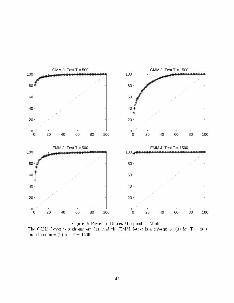
0 20 40 60 80 1000

20

40

60

80

100EMM J−Test T = 500

0 20 40 60 80 1000

20

40

60

80

100EMM J−Test T = 1500

0 20 40 60 80 1000

20

40

60

80

100GMM J−Test T = 500

0 20 40 60 80 1000

20

40

60

80

100GMM J−Test T = 1500

Figure 9: Power to Detect Misspeci�ed Model.The GMM J-test is a chi-square (1), and the EMM J-test is a chi-square (3) for T = 500and chi-square (5) for T = 1500.

42