A study of the

effects of waves on evaporation

from free water

surfaces

Research Report No. 18 • A WATER RESOURCES TECHNICAL PUBLICATION

A study of the effects of waves on evaporation from free water surfaces

prepared by Calvin C. Easterbrook,

Cornell Aeronautical Laboratory, Inc.,

for the Bureau of Reclamation

UNITED STATES' DEPARTMENT OF THE INTERIOR

BUREAU OF RECLAMATION

As the Nation's principal conservation agency, the Department of the Interior has basic responsibilities for water, fish, wildlife, mineral, land, park and recreational resources. Indian and Territorial affairs are other major concerns of America's "Department of Natural Resources., The Department works to assure the wisest choice in managing all our resources so each will make its full contribution to a better United States­now and in the future.

First Printing: 1969

U.S. GOVERNMENT PRINTING OFFICE

WASHINGTON: 1969

For sale by the Superintendent of Documents, U.S. Government Printing Office, Washington, D.C. 20402, or the Chief Engineer, Bureau of Reclamation, Attention 841, Denver Federal Center, Den~~er, Colo. 80225. Price 65 cents.

PREFACE

For several years, the Bureau of Reclamation has conducted research in the use of monomolecular films (monolayers) of fatty alcohols and similar ma­terials placed on water surfaces to retard evaporation. The incentive for this research is to reduce the great evaporation losses from large lakes and reservoirs in the 17 western United States, estimated at more than 14 million acre-feet annually, and at the same time to improve the quality of the water in the lakes and reservoirs.

The Bureau's research program in evaporation re­puction is being carried out at selected field sites and in the Bureau's Engineering and Research Center at Den­ver, as well as through contracts with educational institutions, other government agencies, and com­mercial research organizations. Among these activ­ities is the investigation to determine the quantita­tive relationship between wave and air flow character­istics and the evaporation rate, and to increase under­standing of the microphysical processes that control the rate of mass transport across a water surface. Such an investigation, described in this Research Report, is important because, as the author states, " ... waves

on a water surface have a significant effect on the evaporation rate from that surface".

The work described herein was carried out by Calvin C. Easterbrook of the Cornell Aeronautical Laboratory, Inc., of Cornell University at Buffalo, N. Y., under research contract No. 14-06-D-5764 with the Bureau of Reclamation. The original report was given limited distribution under its designation, CAL Report No. RM-2151-P-1, dated April 15, 1968. As Mr. Easterbrook's research work is of con­tinuing interest to researchers studying the use of monolayers, it is reprinted here as a Bureau of Rec­lamation Water Resources Technical Publication.

Included in this publication is an informative abstract with a list of descriptors, or keywords, and "identifiers". The abstract was prepared as part of the Bureau of Reclamation's program of indexing and retrieving the literature of water resources de­velopment. The descriptors were selected from the Thesaurus of Descriptors, which is the Bureau's stand­ard for listing of keywords.

Other recent issues in the Water Resources Tech­nical Publications group are listed on the inside back cover of this report.

ACKNOWLEDGMENTS

I wish to express sincere appreciation for the assistance and cooperation given by Dr. Bradford Bean, Mr. Ray McGavin, and several other members of the Radio Meteorology Section, Tropospheric Telecommunications Laboratory, of the Environ­mental Science Services Administration. Without the meteorological data supplied by the ESSA group, the CAL study of wave-evaporation interaction at Lake Hefner would not likely have been possible. I also wish to thank the many people from the Bureau of Reclamation for their continued interest in and

support of this work and for their willing assistance during the Lake Hefner field program.

This report has been approved by George E. Mc­Vehil, Head, Dynamic Meteorology Section, and Roland J. Pilie, Assistant Head, Applied Physics Department of the Cornell Aeronautical Laboratory, Inc.

CALVIN C. EASTERBROOK.

iii

CONTENTS Page

Preface___________ _ _ _ _ _ _ _ _ _ _ _ _ _ _ _ _ _ _ _ _ _ _ _ _ _ _ _ _ _ _ _ _ _ _ _ _ _ _ _ _ _ _ _ _ _ _ _ _ _ iii Acknowledgments ____________________________________ --_____________ iii

SuDlDlarY---------------------------------------------------------- 1 Introduction------------------------------------------------------- 3

The wave tank evaporation experiments _______ -- ____________ --_________ 5 Evaporation tank design and instruDlentation_ _ _ _ _ _ _ _ _ _ _ _ _ _ _ _ _ _ _ _ _ _ _ 5

Developn1ent of evaporation tank theory ____ ------ ________ ---- __ --- 7 Results of the wave tank evaporation experiDlents ____ ---- ______ ---- _ 10 Investigation of evaporation controlling DlechanisDlS- _____ ---- __ ---- _ 12 Conclusions_ _ _ _ _ _ _ _ _ _ _ _ _ _ _ _ _ _ _ _ _ _ _ _ _ _ _ _ _ _ _ _ _ _ _ _ _ _ _ _ _ _ _ _ _ _ _ _ _ _ _ _ 21

The Lake Hefner evaporation study___________________________________ 22 Instrumentation at Lake Hefner _______________________ -___________ 22

Dataacqubition------------------------------------~----------- 24 Processing and analysb of Lake Hefner data________________________ 25

Con1parison of the laboratory and field results___________________________ 33

Evaporation estimates and waves______________________________________ 35

Conclusions and recoDlDlendations____ __ _ _ _ _ _ _ _ _ __ _ _ __ __ __ _ _ _ _ _ _ _ _ __ __ _ 39

References--------------------------------------------------------- 41

Appendix:

A. Bridge circuit used for thermistor temperature measuren1ents in wind

tunnel-------------------------------------------------------- 43 B. Solution of wave tank electrical analog____________________________ 45 C. Design and construction details of the wave probe____________________ 47 D. Basic data fron1 the wave tank evaporation experiDlents_______________ 51 E. Reduced Lake Hefner data________________________________________ 53

Abstract----------------------------------------------------------- 58

FIGURES Number

1. Schematic diagram of evaporation tank_____________________________ 5· 2. Evaporation tank in final stages of construction______________________ 6 3. Wave generating assembly________________________________________ 6 4. High capacity fan installation_____________________________________ 6

v

Number Page

5. The return duct observed through fan blades ___ ------_______________ 6 6. Beach trap modification _________________ ----_____________________ 7

7. Electrical analog of evaporation experiment_ ___ ------_______________ 9 8. Normalized specific humidity as a function of time___________________ 10 9. Evaporation coefficient D in feet per second as a function of wind speed

and wave parameter HjT______________________________________ 11

10. Evaporation coefficient as a function of wave parameter for constant

windspeeds-------------------------------------------------- 13 11. Temperature and humidity as a function of time, experiment No. 108__ 14 12. Helium bubble stationary behind wave crest________________________ 15 13. Bubble trajectories over surface with only wind-driven capillary waves

present------------------------------------------------------- 16 14. Bubble trajectories over well-developed waves_______________________ 16 15. Smoke tracers over well-developed waves___________________________ 17 16. Smoke tracers over breaking waves_________________________________ 18 17. Smoke bubble released from under water__________________________ 19 18. Smoke tracers showing reverse flow of air near surface ahead of ap-

proaching wave crest_ ___________ --_____________________________ 20

19. Model of air flow over well-developed waves ___________ ----_________ 21 20. Map of Lake Hefner, Oklahoma City, Okla.________________________ 23

21. Basic wave probe configuration------------------------------------ 24 22. Wave probe installation at Lake Hefner, 1966______________________ 25 23. Wave probe installation at the Mid-lake tower, 1967 _ _ _ _ ____ __ __ __ ___ 26

24. Sample wave spectra, August 1966--------------------------------- 27 25. Evaporation coefficient D as a function of wind speed, Mid-lake tower__ 28 26. Evaporation coefficient D as a function of wind speed, Intake tower_ _ _ _ 29 27. Total wave energy as a function of the 2-meter wind speed____________ 30 28. Wave parameter H/T ru; a function of the 2-meter wind speed_________ 31 29. Evaporation coefficient D as a function of the wave parameter H/T for

the 2-meter level at the Intake tower____________________________ 31 30. Contours of constant D as a function of wave parameter H/T and wind

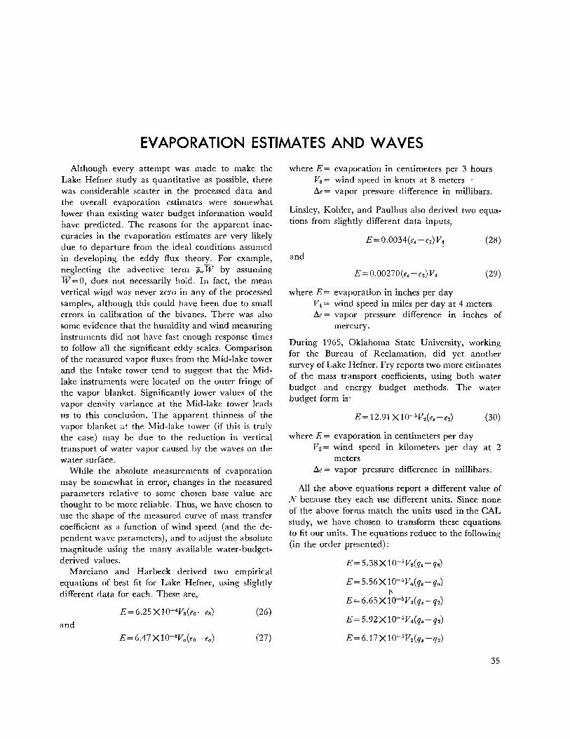
speed-Contours adjusted to fit the Lake Hefner results___________ _ 34 31. Mass transfer coefficient Nasa function of wind speed_______ _ __ ____ _ 37 32. Mass transfer coefficient N as a function of wind speed-Curve adjusted

to fit water budget data_ _ _ _ _ _ _ _ _ _ _ _ _ _ _ _ _ _ _ _ _ _ _ _ _ _ _ _ _ _ _ _ _ _ _ _ _ _ _ _ 38

A-1. Schematic diagram of pulsed thermistor bridge_____________________ 43 B-1. Electrical analog of evaporation experiment________________________ 45 C-1. Block diagram of probe system __________________________ --------- 47 C-2. Schematic diagram of wave probe system__________________________ 48 C-3. Wave probe calibration-curve____________________________________ 49 C-4. Wave measuring probe__________________________________________ SO

vi

SUMMARY Experiments performed in the laboratory and

measurements made in the field show that waves on a water surface have a significant effect on the evapo­ration rate from that surface.

The laboratory measurements were made using a large wave tank-wind tunnel combination in which both wind speed and wave parameters could be con­trolled. Waves were generated at one end of the tank by a hydraulically driven paddle, and dissipated at the other end on a gradually sloped "beach." In this way, wave conditions approaching those developed on large bodies of water (fetches up to a mile or more) could be duplicated.

Results of the tank experiments indicated that for certain combinations of wind speed and well-de­veloped waves, the evaporation rate was less than that measured under similar wind speed conditions with po waves present. Subsequent investigation of air flow over the waves showed that significant changes occurred as wave heights were increased. Regions of dead air were observed to the lee of the

wave crests, and vortices appeared in the wave troughs. The partially trapped air apparently forms an effective barrier to the vertical transport of water vapor.

As a follow-up to the laboratory work, wave and evaporation measurements were made at Lake Hefner in Oklahoma. Evaporation rates were com­puted from wind and moisture measurements by the eddy flux method, and correlated with wave data. The relationships so derived display characteristics very similar to those found in the laboratory.

The short-period mass transport data obtained during the Lake Hefner experiments were combined and adjusted to fit previoUsly measured evaporation coefficient relationships derived from water and energy budget measurements. The resulting evapo­ration coefficient curve is believed to provide an improved measure of the "instantaneous" evapora­tion rate from Lake Hefner under given conditions of wind speed, water surface temperature, and ambient humidity.

1

INTRODUCTION

Many methods and equations have been derived over the past 100 years for estimating the amount of ·evaporation taking place from a free water surface. Some of these relationships are quite complex, re­quiring a number of precise meteorological measure­ments. Others, such as the simple mass transport equation investigated in this study, require only a few basic measurements, are easy to apply, and for these reasons have been widely used. Marciano and Harbeck1 have shown that complex equations such as that of Sutton are little better in practice than the much simplified expressions which usually reduce to a form of the empirically derived mass transport equation,

E=NVa(e,-ea) (1)

where E= evaporation rate Va= mean wind speed at level a e, = saturation vapor pressure at temperatm e

of the water surface ea = mean vapor pressure at level a

N = constant.

While equation (1) is a simple expression which apparently gives accurate estimates of evaporation amounts when applied over long periods of time, it can be defended on physical grounds as well. Equa­tion (1) can be considered to be a simplified one­dimensional diffusion equation of the form

aq E=K­oz

where E = flux of q in the z direction

iJq d" f . d" • - = gra tent o q m 1rect10n z iJz

K = diffusion coefficient.

(2)

In the free atmosphere, it is known that eddy diffusion by turbulence is much greater than molecu­lar diffusion. Thus, the coefficient in the diffusion equation becomes the eddy diffusion coefficient Kw

1 References in this report are listed on page 41.

for water vapor transport. Since the gradient of q must be continuous near the water surface, we can write

(2a)

which must be corr~ct at some particular (but in general unknown) height in the region ~. Equation (2) can then be written

!J.q E=Kw­

~ (3)

where Kw is the value of the diffusion coefficient ap­propriate to the height where equation (2a) holds.

If we consider the layer of air between the water surface and some height z, we can then write

E=D(q.-q.) (4)

where D=Kw z

D, then, is a measure of the eddy diffusivity for the layer (0-z) and, as such, is dependent on the height z and the characteristics of the boundary layer turbulence. The primary factor which governs turbulence intensity near the surface is wind speed. If we postulate a linear dependence of D on wind speed V ., we can express the eddy diffusion equation as

E=NV,(q.-q.) (5}

which is exactly the empirical form of the mass transport equation.

The more complex evaporation equations attempt to express D analytically as a function of the many factors which influence turbulence. However, to the best of our knowledge, no attempts have been made to relate D to wave conditions, which may have an important effect on turbulence structure over the water. There are several ways in which waves might affect evaporation. First, we might think that in­creasing waves may constitute an increasingly rough surface and thus increase the turbulent transport of

3

water vapor. Also, the existence of bubbles, breaking on the wave crests, might constitute a significant de­crease in the surface resistance to mass flux, thus in­creasing evaporation. Associated with this latter mechanism is another which might be even more im­portant; that is, the creation of a vapor source above z = 0 due to spray blown off breaking waves.

It is also possible to envision an effect opposite to the first suggestion above: instead of waves making the surface a~rodynamically more rough, just the opposite may be true. A suggestion along these lines has been proposed by Stewart. Stewart presents ar­guments to show that traveling and developing waves on a water surface may give rise to an or­ganized air flow pattern near the surface. This or­ganized flow, while being able to transport mo­mentum, would act as a barrier to heat and mass transport. A further argument related to the above is suggested by a postulate put forward by Phillips. Phillips found that waves develop most rapidly by a resonance mechanism which occurs when a compo­nent of the surface pressure distribution moves at the same speed as the free surface wave with the same wave number. Phillips' results suggest that certain combinations of wave conditions and wind speed might favor the development of organized flow as discussed by Stewart.

Because of the many unknowns in the evaporation process and its relation to waves on the evaporating surface, Cornell Aeronautical Laboratory undertook

4

a combined laboratory and field study of wave effects on evaporation for the Bureau of Reclamation. The study began in September 1965 and continued through January 1968 under two extensions to the original contract. The overall objectives of the work were as follows:

1. Determine the quantitative relationship between wave characteristics, air flow characteristics, and evaporation rate.

2. Investigate the microphysical processes that control the rate of mass transport across the water surface and the way in which these processes change with wave activity.

3. Develop methods for applying laboratory re­sults to field situations.

4. Develop a general evaporation prediction tech­nique and formulate simple expressions that tnake use of data from routinely available observations to obtain an estimate of the evaporation loss from un­treated open water surfaces.

The work has progressed in two separate phases. Phase 1, completed in July 1966, consisted entirely of laboratory measurements and was directed mainly toward objectives 1 and 2. Phase 2 was a field study of evaporation processes at Lake Hefner, and was aimed at satisfying objectives 3 and 4. This document is the final report under the contract and describes the results of all work performed during the contract period.

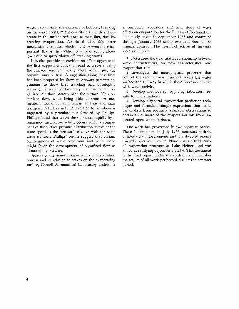
THE WAVE TANK EVAPORATION EXPERIMENTS

The laboratory experiments described herein were carried out in a wave tank, originally constructed at C:AL for use in the study of water waves by Doppler radar. The wave tank consists of a large open trough, 40 feet long, 4 feet wide, and 3 feet deep with an eJectrically driven paddle at one end of the tank. The paddle generates waves which travel down the trough and are dissipated on a gently sloping "beach".

For the evaporation experiments the wave tank was enclosed and a large fan was installed to circu­late air over the water surface. Instruments were ip.stalled to make measurements of the moisture con­tent, temperature, and speed of the air moving over the evaporating surface. Details of the evaporation !:iXperiments are given below.

Evaporation Tank Design and Instrumentation

A diagram of the combination wave and evapora­tion tank is shown in figure 1. A return duct con­structed on top of the existing wave tank carries the

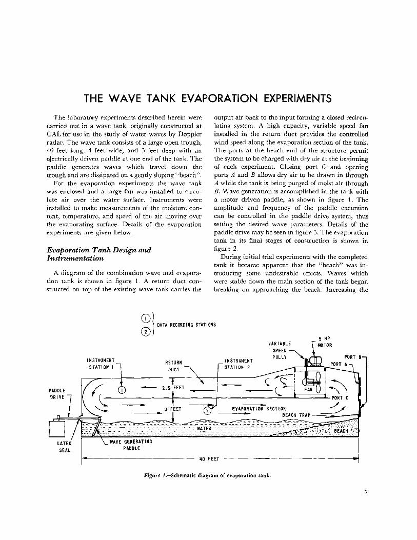
output air back to the input forming a closed recircu­lating system. A high capacity, variable speed fan installed in the return duct provides the controlled wind speed along the evaporation section of the tank. The ports at the beach end of the structure permit the system to be charged with dry air at the beginning of each experiment. Closing port C and opening ports A and B allows dry air to be drawn in through A while the tank is being purged of moist air through B. Wave generation is accomplished in the tank with a motor driven paddle, as shown in figure 1. The amplitude and frequency of the paddle excursion can be controlled in the paddle drive system, thus setting the desired wave parameters. Details of the paddle drive may be seen in figure 3. The evaporation tank in its final stages of construction is shown in figure 2.

During initial trial experiments with the completed tank it became apparent that the "beach" was in­troducing some undesirable effects. Waves which were stable down the main section of the tank began breaking on approaching the beach. Increasing the

CDJ DATA RECORDING STATIONS

0

SEAL

INSTRUMENT STATION I

WAVE GENERATING PADDLE

RETURN

~0 FEET

INSTRUMENT STATION 2

---

FiguTe 1.-Schematic diagram of evapotation tank.

5

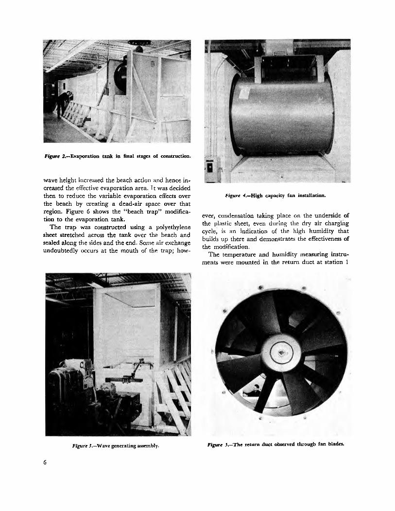
Figure .2.-Evaporation tank in final stages of construction.

wave height increased the beach action and hence in­creased the effective evaporation area. It was decided then to reduce the variable evaporation effects over the beach by creating a dead-air space over that region. Figure 6 shows the "beach trap" modifica­tion to the evaporation tank.

The trap was constructed using a polyethylene sheet stretched across the tank over the beach and sealed along the sides and the end. Some air exchange undoubtedly occurs at the mouth of the trap; how-

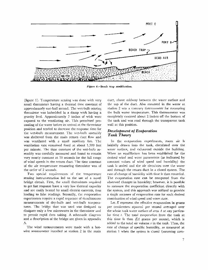
Figure J.-Wave generating assembly.

6

Figure 4.-High capacity fan installation.

ever, condensation taking place on the undei"Side of the plastic sheet, even during the dry air cli~tgirig cycle, is an indication of the high humidity thai builds up there and demonstrates the effectiveness of the modification.

The temperature and humidity measuring instru­ments were mounted in the return duct at station 1

Pipe J.-The return duct oblerved through fan blades.

PORT C

Figure 6.-Beac:h trap modification.

{figure 1). Temperature sensing was done with very small thermistors having a thermal time constant of approximately one-half second. The wet-bulb sensing thermistor was imbedded in a damp wick having a gravity feed. Approximately 2 inches of wick were exposed to the ventilating air. This permitted pre­cooling of the water before its arrival at the thermistor position and tended to decrease the response time for the wet-bulb measurement. The wet-bulb assembly was sheltered from the main return duct flow and was ventilated with a small auxiliary fan. The ventilation rate remained fixed at about 1,500 feet per minute. The time constant of the wet-bulb as­sembly was carefully measured and found to remain very nearly constant at 10 seconds for the full range of wind speeds in the return duct. The time constant of the air temperature measuring thermistor was of the order of 2 seconds.

Two special requirements of the temperature sensing instrumentation led to the use of a novel bridge circuit. First, the small thermistors required to get fast response have a very low thermal capacity and are easily heated by small electric currents, thus leading to false readings. Secondly, the evaporation experiments require a rapid sequence of simultaneous measurements of dry-bulb and wet-bulb tempera­tures. The bridge that was used was designed to dissipate only a few microwatts in the thermistor and to permit rapid data taking. A schematic diagram and a description of the bridge are given in appendix A.

The wind measurements were made with a hot­wire anemometer installed at station 2 in the main

duct, about midway between the water surface and the top of the duct. Also mounted in the water at station 2 was a mercury thermometer for measuring the bulk water temperature. This thermometer was completely emersed about 2 inches off the bottom of the tank and was read through the transparent tank wall at this position.

Development of Evaporation Tank Theory

In the evaporation experiments, room air is initially drawn into the tank, circulated over the water surface, and exhausted outside the building. When an equilibrium has been established for the desired wind and wave parameters (as indicated by constant vah,1es of wind speed and humidity) the tank is sealed and the air circulates over the water and through the return duct in a closed system. The rate of change of humidity with time is then recorded. The evaporation rate can be computed from the observed changes in humidity;· however, it is possible to measure the evaporation coefficient directly with the system, and this approach was utilized to provide a single measure of evaporation rate for each desired combination of wind speed and wave state.

Let E represent the effective evaporation in grams per centimeters squared per second averaged over the whole tank water surface of area A at any particu­lar time t. The total evaporation from the tank at this time is then EA grams per second, which is added to the total air volume v in the tank. Thus, the rate of change of specific humidity, as measured at station 1 when the system is closed (assuming com-

7

plete mixing in the return duct), is

or

dq AE -d = - grams per gram per second

t vp

E= vpdq A dt

(6)

(7)

where p = density of air q= specific humidity.

Equation (7) then permits a computation of evapora­tion rate from the slope of the measured q(t) curve if the air volume in the tank and the effective water surface area are known.

Let us next consider the simple bulk aerodynamic evaporation equation

E=pN(q.-q .. )V,. (8)

where E= evaporation rate, grams per centimeter squared per second

p= air density, grams per centimeter cubed q. = specific humidity of saturated air at the

temperature of the water surface, grams per gram

q .. = specific humidity at some fixed level a V .. = wind velocity at level a N = evaporation coefficient.

The evaporation coefficient N is normally treated as a constant but it is known to be dependent upon atmospheric stability and, as shown in our pre­liminary · experiments, is dependent upon wave structure. Furthermore, equation (8) breaks down when the wind velocity approaches zero, since evaporation does not stop entirely under zero wind velocity provided that q,.<q •. We elect, therefore, to incorporate the wind velocity dependence into the factor D. D now has units of velocity and is a func­tion of V as well as other parameters describing the wave characteristics and turbulent transport. Equa­tion (8) then may be written in the form

E=pD(q.-q .. ) (9)

In the wave tank experiment, equation (9) can only be applied on an instantaneous basis since q(J and E change with time. Thus, for the tank experi­ment we can write equation (9) as

E(t) = pD[q.-q(t)] (10)

Here, q(t) is the instantaneous value of q measured at station 1 in the tank. If we combine equations (7)

8

and (10) and differentiate with respect to t, we ob­tain the differential equation

v d2q dq --+D- =0 A dt 2 dt

(11)

This result is obtained under the assumptions that q. is constant (water temperature remains constant) and D is a constant for a particular experiment. Equation (11) has the solution

q(t) =q. [ 1- exp (- D:t) J (12)

for the boundary conditions of our experiment, i.e.,

q=O for t=O

q=q, for t= oo

v The quantity DA is the time constant of the evapora-

tion experiment under the particular wave and air velocity conditions set and we can write

v D=­

Ar

where v = effective volume of air in tank A = effective evaporation area

(13)

D= evaporation coefficient (with units of velocity)

r = time constant of experiment.

Thus, D can be computed directly from measurement of the experimental time constant.

There are two sources of error inherent in the actual tank apparatus that are not accounted for in the simple solution above. First, the humidity meas­uring instruments at station 1 do not respond in­stantaneously, but have a finite time constant as dis­cussed in the preceding section on instrumentation. Also, the tank is not completely air tight. There is a small amount of air leakage around the fan bearings, the paddle drive seal, and the intake and exhaust ports. It is possible to take these effects into account in the final analysis of the tank experiment.

Considering the evaporation process and the re­sulting solution, equation (12), it is readily seen that the recirculating tank experiment is directly anal­ogous to charging a capacitor through a resistance. Here the time constant vj DA is equivalent to RC in the electrical circuit, R is equivalent to 1/DA, and C is represented by the t~nk volume v. With this in mind we can set up an electrical analog of the evapo-

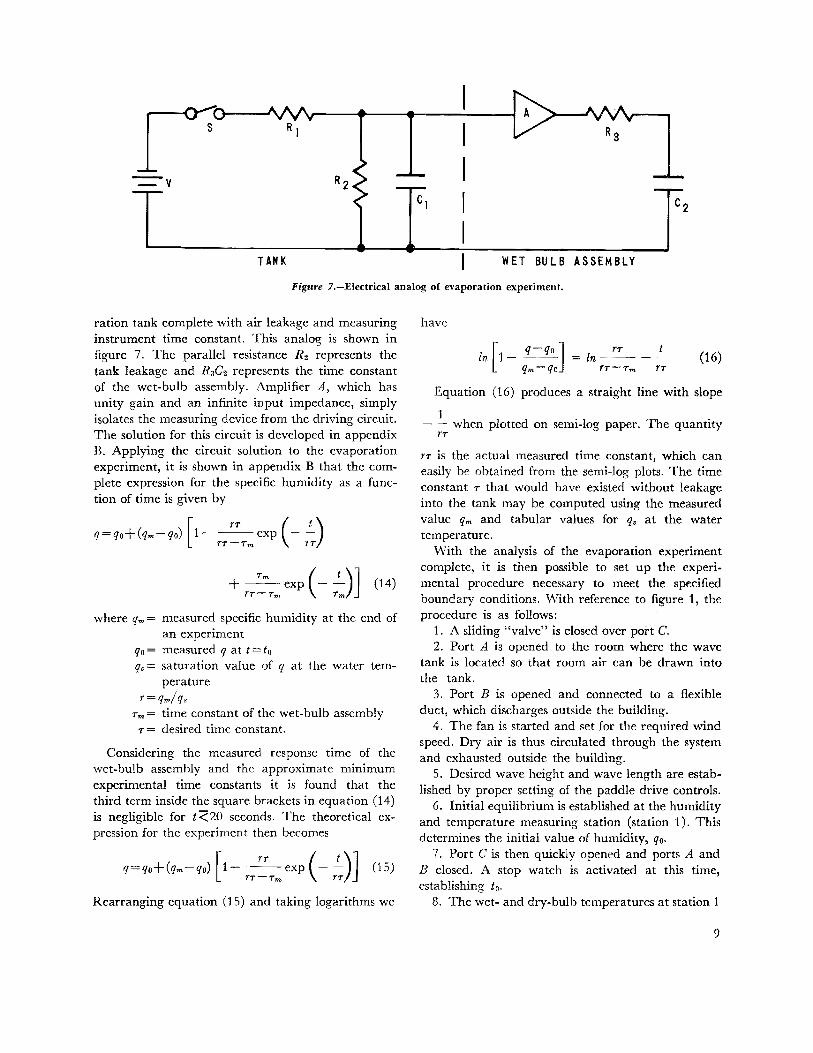
--=-v

TANK WET BULB ASSEMBLY

Figure 7.-Electrical analog of evaporation experiment.

ration tank complete with air leakage and measuring instrument time constant. This analog is shown in figure 7. The parallel resistance Rz represents the tank leakage and R3C2 represents the time constant of the wet-bulb assembly. Amplifier A, which has unity gain and an infinite input impedance, simply isolates the measuring device from the driving circuit. The solution for this circuit is developed in appendix B. Applying the circuit solution to the evaporation experiment, it is shown in appendix B that the com­plete expression for the specific humidity as a func­tion of time is given by

q=qo+(q,.-qo) [1- _!2_exp (- !___) TT-Tm TT

+ ~ exp (- .!._)] (14) TT-Tm Tm

where q ... = measured specific humidity at the end of an experiment

q0 = measured qat t=to q. = saturation value of q at the water tem­

perature r=q,./q.

T,..= time constant of the wet-bulb assembly T = desired time constant.

Considering the measured response time of the wet-bulb assembly and the approximate minimum experimental time constants it is found that the third term inside the square brackets in equation (14) is negligible for e:<:zo seconds. The theoretical ex­pression for the experiment then becomes

q=qo+(q,.-qo) [1- _!2_ exp (- !___)] (15) TT-Tm TT

Rearranging equation (15) and taking logarithms we

have

T'T t =ln---- (16)

rT-Tm TT

Equation (16) produces a straight line with slope

- .!._ when plotted on semi-log paper. The quantity TT

TT is the actual measured time constant, which can easily be obtained from the semi-log plots. The time constant T that would have existed without leakage into the tank may be computed using the measured value q.,. and tabular values for q. at the water temperature.

With the analysis of the evaporation experiment complete, it is then possible to set up the experi­mental procedure necessary to meet the specified boundary conditions. With reference to figure 1, the procedure is as follows:

1. A sliding "valve" is closed over port C. 2. Port A is opened to the room where the wave

tank is located so that room air can be drawn into the tank.

3. Port B is opened and connected to a flexible duct, which discharges outside the building.

4. The fan is started and set for the required wind speed. Dry air is thus circulated through the system and exhausted outside the building.

5. Desired wave height and wave length are estab­lished by proper setting of the paddle drive controls.

6. Initial equilibrium is established at the humidity and temperature measuring station (station 1). This determines the initial value of humidity, qo.

7. Port C is then quickly opened and ports A and B closed. A stop watch is activated at this time, establishing to.

8. The wet- and dry-bulb temperatures at station 1

9

1.0 ......... ~""" :::-c..

' ~~ ~ "4" ......... .......... -...a

""" ,.,....,_,

....... """-( '-......,

'"' ~ :--..... ~ ~ ~ ""' ~ -............. ~

~ ~ ~~ ~ -a...~ '-...!::?"-- 2o

~

~ K 38 p-_#as ~ ~ ~ ~ "' ~ • 10 ' i

"' ·~ ......... b. ~

" "He ,....._#sa 1--~ '4-. "l'c.

' ~ f-- 1135 - NO WAVE; V = 175 FT/MI N

~~I 'f'.-ed' ........ .,., 1153 - BREAKING WAVES: V = 175 FT/MIN f'.."~

f-- 632 • NO WAVES; V = 500 FT/MIN "" 11~~- BREAKING WAVES; V = 900 FT/MIN Rj,l'j,l'

.01 0 2 3 5 6

TIME IN MINUTES

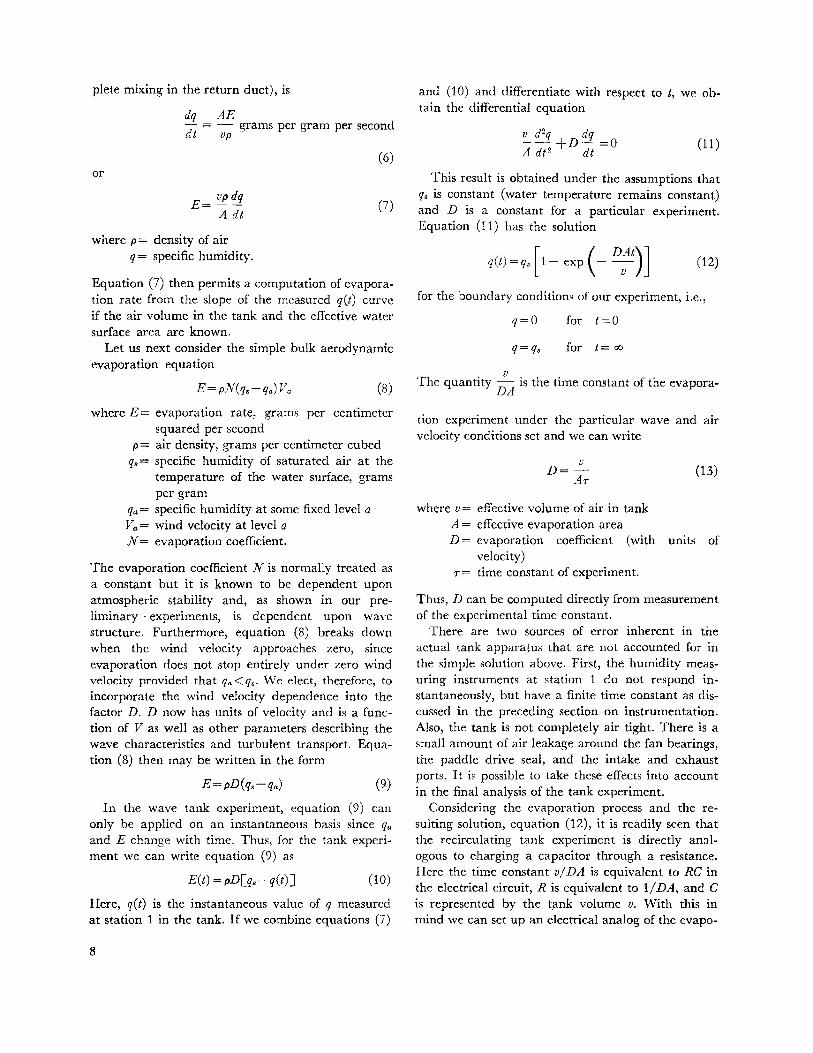
Figuf'e B.-Normalized specific humidity as a function of time.

are recorded every 20 seconds during the first few minutes of each experiment, and then less frequently as the evaporation rate falls off due to the increase in moisture content of the air. The maximum equilib­rium value qm is obtained when the wet-bulb tem­perature ceases to increase.

9. The average wind speed at station 2 during the experiment is recorded, along with the water tem­perature. The barometric pressure at the time of the experiment is also recorded.

. q(t) -qo. 10. The quant1ty 1- --- 1s computed for each

qm-qo

data point and the values are plotted on semi­logarithmic graph paper. The slope of the resulting straight line then represents the time constant of the experiment. Note that the initial point q0 is not used in determining the appropriate straight line through the data points. This is in keeping with the approximation used when neglecting the last term of the solution, equation (14).

10

Results of the Wave Tank Evaporation Experiments

A total of 108 experiments was completed in the wave tank, producing 76 useful samples of data. The first 32 data runs were performed during the "shake­down" period of the evaporation-wave tank while modifications were still being made; hence, these data were not used in the final analysis.

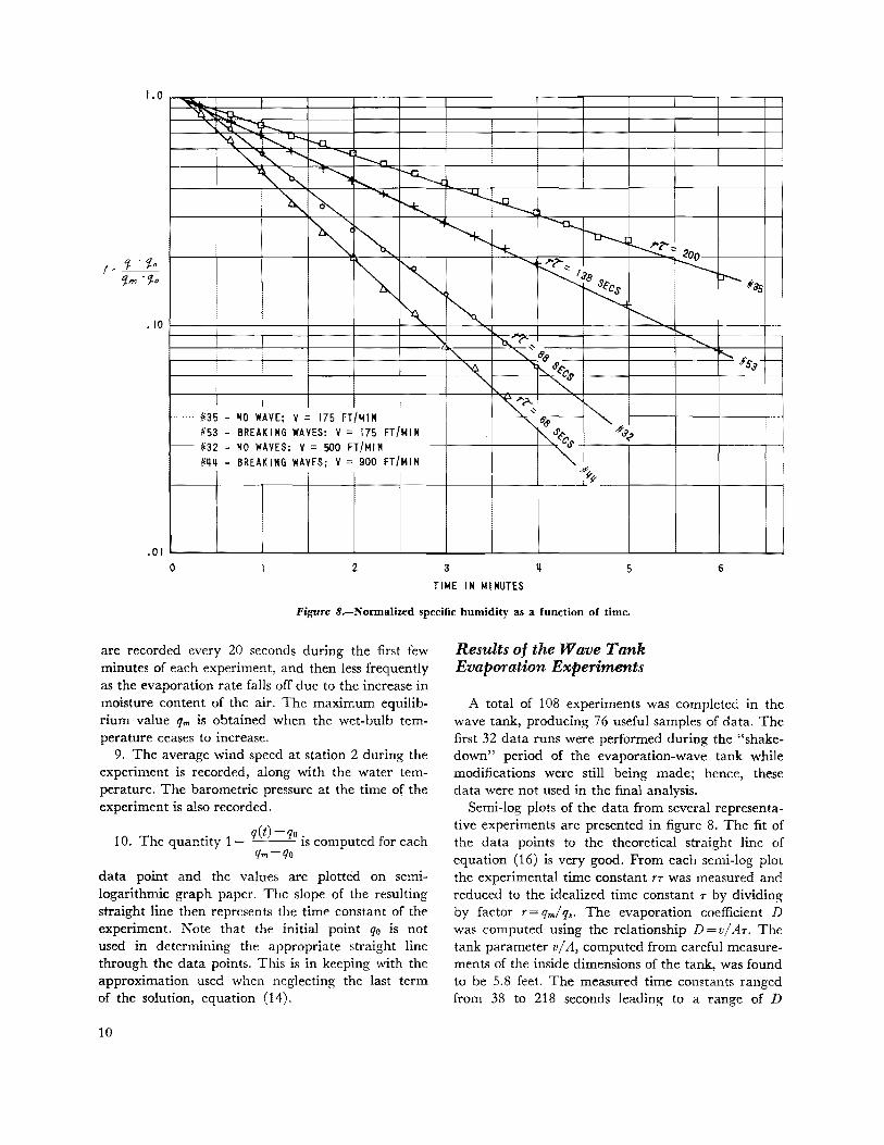
Semi-log plots of the data from several representa­tive experiments are presented in figure 8. The fit of the data points to the theoretical straight line of equation (16) is very good. From each semi-log plot the experimental time constant rr was measured and reduced to the idealized time constant r by dividing by factor r=qm/q,. The evaporation coefficient D was computed using the relationship D=v/Ar. The tank parameter v /A, computed from careful measure­ments of the inside dimensions of the tank, was found to be 5.8 feet. The measured time constants ranged from 38 to 218 seconds leading to a range of D

u

" .,

o. 7

0.6

0.5

..........

--,_

........_ r--......_ -1--

!-...... ~

....___

1--- --r---- ----t----. 1-- "" ...........

11'-. -- ,;:>.

-- '\ I -~ ~ - II

I ~ .... - ...... J

...........

~ ~---.. ., I v I I ~·

1 II L_ v / / -­.... .... - o. ~ ""' ~r-.... 1'\ . ...

_, ) .. J J v ~ v v L_ / // _L ,_ -­:z:

"" w t;:; ""

_ .... """

.... I v / v L_ v v L_ L v/ L v ~ ... J I 1/ v L_ v v / L_ L ........ / / ~

: 0.3 ... w ,.. ~ '

I v I I v / v ~ L L L L_ L J

\ I I 1/ I I v I j_ v vi_ _/__ _j_ _j_ 0.2

1/ l oL o.b 1/ L !. I/ l l ./ f. / f-D 0.03-0.0~- r--0.06- r-0.08-0l109- O'\Q_O'i\1_0l_Q,i OJ 015-~16 i

0.1

1\ \ \ \ \ 1\ \ ~ ~ \ \ \ \ \ \ ' 1\ \ '\ \

~ 1\ ' [\. oLt 2 1\. ~ [\.. ~ ~

3 ~ 5 6 7 8 9 10 11 12 13 1q 15 16 17 18 19 20 21 22 23 0

WIND SPEED, ft/ sec

Figure .9.-Evaporation coeffident D in feet per second as a function of wind speed and wave parameter H/T.

factors from 0.027 to 0.152 foot per second. All basic data from the final 76 experiments were compiled and are included in appendix D of this report.

During the data analysis, two wave parameters were considered: the wave steepness parameter H/L (wave height to length ratio) and the wave height to period ratio H/ T. Correlation of either of these two parameters with the evaporation data produced essentially the same results. We have chosen to present the final results in terms of the wave param­eter H/ T. This parameter seems more appropriate for two reasons: (1) wave period is easier to measure than wave length, and (2) the parameter H/T con­tains information on wave velocity as well as wave length, both of which may be important outside the laboratory.

Figure 9 shows the final results of the wave tank analysis. This diagram was constructed by plotting the measured values of the evaporation coefficient D at the appropriate location in the Hj T, V field and drawing contours of constant D. The resulting iso­pleths display several interesting characteristics. The first property one may note is that for a given value

of H/ T the evaporation coefficient is a nearly linear function of wind speed. This result is not surprising in view of the success with which the empirical equa­tion {8) has been applied in the past. Secondly, it is evident from figure 9 that D is not constant for a given wind speed, but is also a function of wave characteristics. It is here that a rather unexpected result appears. Over a certain range of wave char­acteristics, the evaporation rate actually decreases with increasing wave height to period ratio. (This result is discussed in some detail later.) Finally, there is a break-over zone (shown on figure 9 as a dotted line) above which the D factor increases rapidly with increasing H/T. This zone roughly coincides with the initial appearance of a visible curl on the wave crest, indicating wave breaking. The correspondence can be described only as approximate because the curl was never observed with H/T smaller than 0.5, but the evaporation data indicate that at low wind velocities the break-over zone does occur at values of H/T as small as 0.3. In previous work we have noted that other properties of waves in still air approach values characteristic of breaking waves before a

11

visible curl appears. In particular, Mee reported similar variations in the Doppler spectrum of sea clutter.

Having obtained evaporation data in the labo­ratory, it is of interest to compare the results with evaporation measurements made in the field. One sample of evaporation data with which we can com­pare our results is that obtained in the study of Lake Hefner for the Bureau of Reclamation by the Navy Electronics Laboratory (Marciano and Harbeck). The empirical equation of best fit to the data given in this report is

E= 6.25X 10-4ua(eo-es) (17)

where E= evaporation rate in centimeters per 3 hours

u8 = 8-meter wind speed in knots eo= saturation vapor-pressure at the water

surface temperature in millibars ea= vapor pressure at 8 meters.

The evaporation equation used in the CAL study is

(18)

where E= evaporation rate in grams per centimeter squared per second

p = density of air in grams per centimeter cubed

qo = saturation specific humidity at water sur­face temperature

qa = measured specific humidity at a point in the return duct of the wave tank.

If we use the relationship

0.622e q:::<--

p (19)

where p = atmospheric pressure in millibars e = vapor pressure in millibars

and make the necessary transposition of units, we can reduce the tank evaporation equation to

E=0.244D(e0 -e4 ) centimeters per 3 hours (20)

For a wind speed of 10 knots and a wave parameter H/ T = 0.4, for example, the two equations agree within a factor of 4, the larger evaporation rate being given by the tank-developed equation. This result is not unreasonable if it is remembered that the N.E.L. equation uses parameters measured at 8 meters, whereas the CAL wave tank equation was derived from measurements made within one-half meter of the surface. The two equations cannot be reconciled precisely without detailed knowledge of the wind and humidity profiles both in the field and in the

12

wave tank. However, the factor of 4 can be ac­counted for using reasonable values of vertical wind shear and moisture gradient. A detailed comparison is not really justified since it is clear that air flow properties in the tank cannot fully duplicate those in the atmosphere. The experiments have been con­ducted to determine the variability of evaporation with wave state rather than to measure precise evaporation rates for application to field situations.

Investigation of Evaporation Controlling Mechanisms

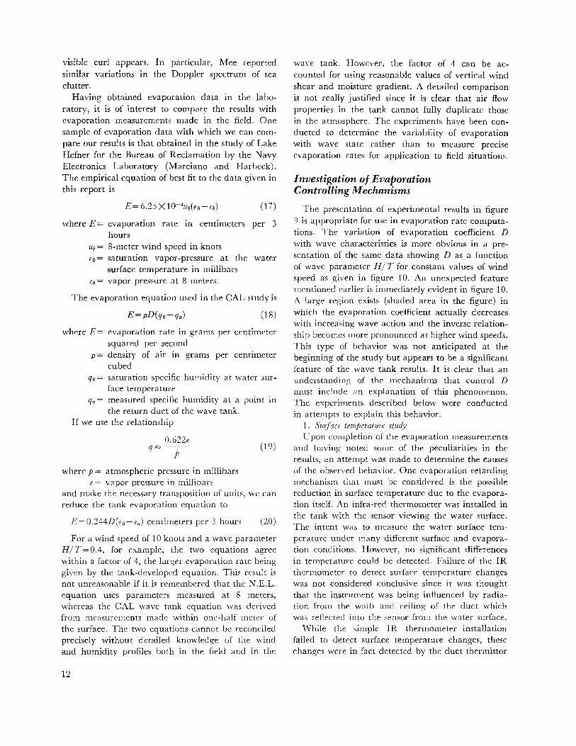
The presentation of experimental results in figure 9 is appropriate for use in evaporation rate computa­tions. The variation of evaporation coefficient D with wave characteristics is more obvious in a pre­sentation of the same data showing D as a function of wave parameter H/T for constant values of wind speed as given in figure 10. An unexpected feature mentioned earlier is immediately evident in figure 10. A large region exists (shaded area in the figure) in which the evaporation coefficient actually decreases with increasing wave action and the inverse relation­ship becomes more pronounced at higher wind speeds. This type of behavior was not anticipated at the beginning of the study but appears to be a significant feature of the wave tank results. It is clear that an understanding of the mechanisms that control D must include an explanation of this phenomenon. The experiments described below were conducted in attempts to explain this behavior.

1. Surface temperature study Upon completion of the evaporation measurements

and having noted some of the peculiarities in the results, an attempt was made to determine the causes of the observed behavior. One evaporation retarding mechanism that must be considered is the possible reduction in surface temperature due to the evapora­tion itself. An infra-red thermometer was installed in the tank with the sensor viewing the water surface. The intent was to measure the water surface tem­perature under many different surface and evapora­tion conditions. However, no significant differences in temperature could be detected. Failure of the IR thermometer to detect surface temperature changes was not considered conclusive since it was thought that the instrument was being influenced by radia­tion from the walls and ceiling of the duct which was reflected into the sensor from the water surface.

While the simple IR thermometer installation failed to detect surface temperature changes, these changes were in fact detected by the duct thermistor

WIND SPEED 0.15

0.1 ~

0.13

0.12

0.11

0.10

u 0.09 CD rb -+'

'+- 0.08 a:: 0 1-u 0.07 cC 1.1..

Q

0.06

0.05

o.oq

0.03

0.02

0.01 0 0.1 0.2 0.3 o.~ 0.5 o. 6 0.7

WAY E PARAMETER H/ T, ft/ sec

Figure 10.-Evaporation coeflic:ient as a function of wave parameter for constant wind speeds.

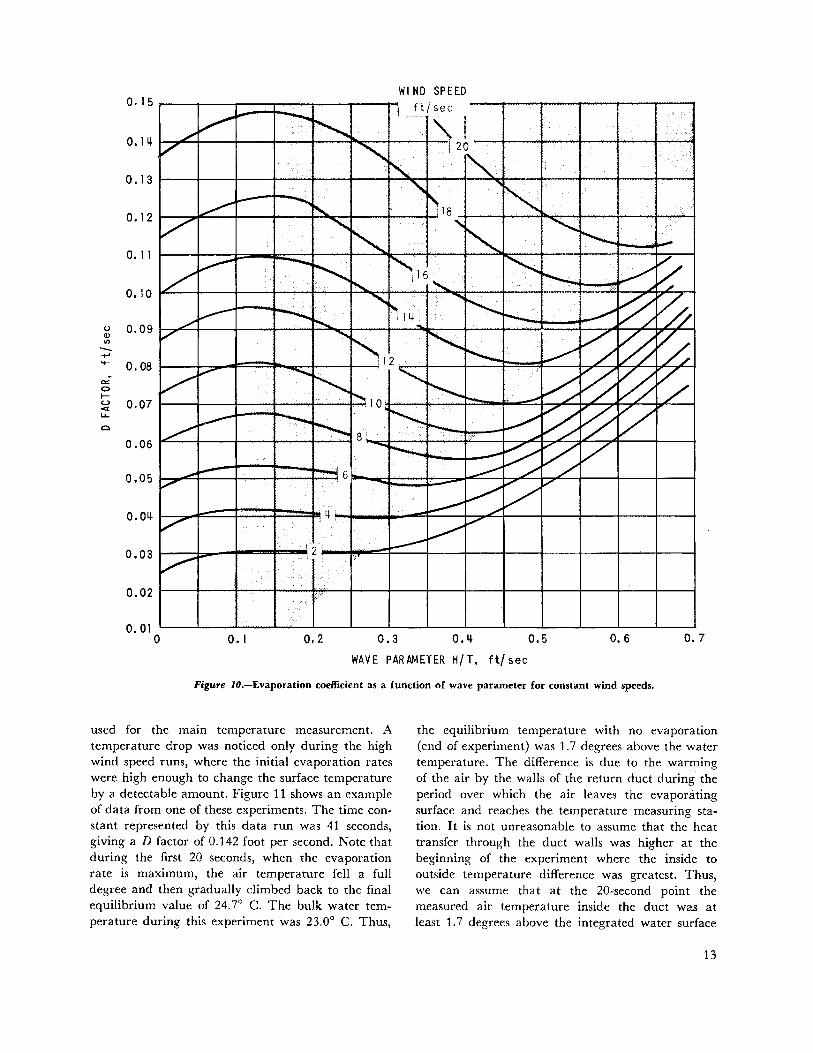
used for the main temperature measurement. A temperature drop was noticed only during the high wind speed runs, where the initial evaporation rates were high enough to change the surface temperature by a detectable amount. Figure 11 shows an example of data from one of these experiments. The time con­stant represented by this data run was 41 second~,

giving aD factor of 0.142 foot per second. Note that during the first 20 seconds, when the evaporation rate is maximum, the air temperature fell a full degree ·and then gradually climbed back to the final equilibrium value of 24.7° C. The bulk water tem­perature during this experiment was 23.0° C. Thus,

the equilibrium temperature with no evaporation (end of experiment) was 1.7 degrees above the water temperature. The difference is due to the warming of the air by the walls of the return duct during. the period over which the air leaves the evaporating surface and reaches the temperature measuring sta­tion. It is not unreasonable to assume that the heat transfer through the duct walls was higher at the beginning of the experiment where the inside to outside temperature difference was greatest. Thus, we can assume that at the 20--second point the measured air temperature inside the duct was at least 1. 7 degrees above the integrated water surface

13

26

lPECI F! C HUJI Dl TY

20

18

~ ~

-"""

/ ,.....

v \ /

16

lit Cl

.::.:.

12 -e Cl

>-10 .....

<.) 0

w a= ::::. ..... -< a= ..... 0.. ::E 25 .....

1\ J {

TEMPERATURE

0

% ::>

8 :z:: (.)

..... a=

-<

v :.,.......,.-~--~ ,_ _____

--... --1'-- ~--~ u..

!,

21t 0

\ r--

, ..... '1

.~"' ~,.

.,.~ 6 (.) w a.. (,1)

It

2

0 2 3 5

TIME IN MINUTES

Figure 11.-Temperature and humidity as a function of time, Experiment No. 108.

temperature. This assumption is certainly on the conservative side, but it still places the water surface temperature at 22.5° C, or 0.5 degree below the bulk water temperature. Although the temperature drop is small and not likely to be significant in re­ducing evaporation ratJs, its presence is rather sur­prising in view of the violent water surface agitation by wind and waves taking place during the experi­ment.

2. Air flow tracing Another possible reason for the decrease in evapo­

ration rate with increasing wave steepness is the reduction of vertical mass transport due to modifica­tion of the air flow and turbulence characteristics. In order to investigate this postulate, apparatus was set up in the wave tank to inject tracers into the air stream above the water.

The first method used was to inject neutrally buoyant soap bubbles inflated with helium into the air flow above the water (Schooley). Movies were taken with a 16 mm camera running at approxi­mately 50 frames per second. Displaying these pictures at 8 frames per second uncovered some inter­esting flow structure around well-developed waves.

14

Figure 12 is an example of several consecutive frames showing a bubble in a typical stationary position (relative to the wave) just in the lee of a wave crest. The same sequence shows other bubbles at higher altitudes moving with the wind speed, which was 2 to 3 times the wave phase velocity. Similar data were analyzed frame by frame, plotting bubble trajectories. Typical trajectories over small, wind-driven capillaries are shown in figure 13. Note the fairly uniform motion at all levels. Figure 14, in turn, shows bubble trajec­tories in the presence of well-developed waves. Note that the upper flow is relatively undisturbed but the low level circulation is completely changed. Circula­tion patterns coupled to the wave profile are im­mediately evident.

In another series of experiments, air motions were traced by releasing chemical vapor plumes near the waves and photographing the plumes with the camera. Air, saturated with titanium tetrachloride (TiC14), was pumped through the same bubble generators used in the bubble tests. TiCl4 reacts with water vapor to form a fairly dense white cloud of hydrogen chloride. The· fumes are toxic, of course, but the experiments were carried out in the sealed

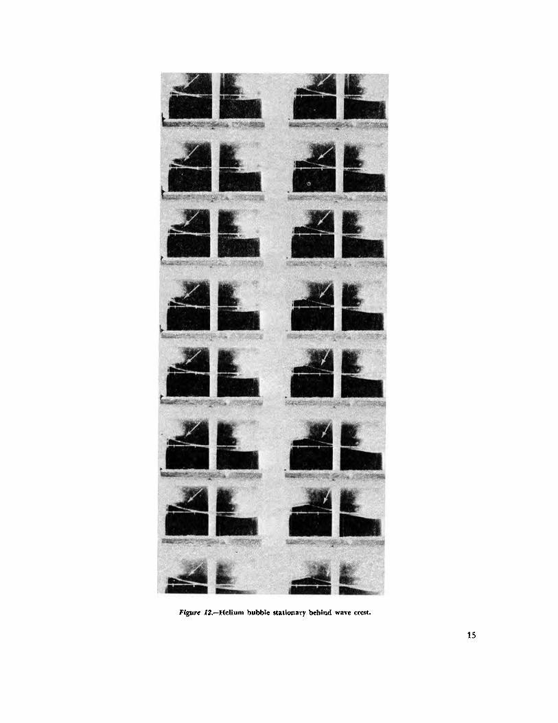
Figure 1.2.-Helium bubble sllitionary behind wave crest.

15

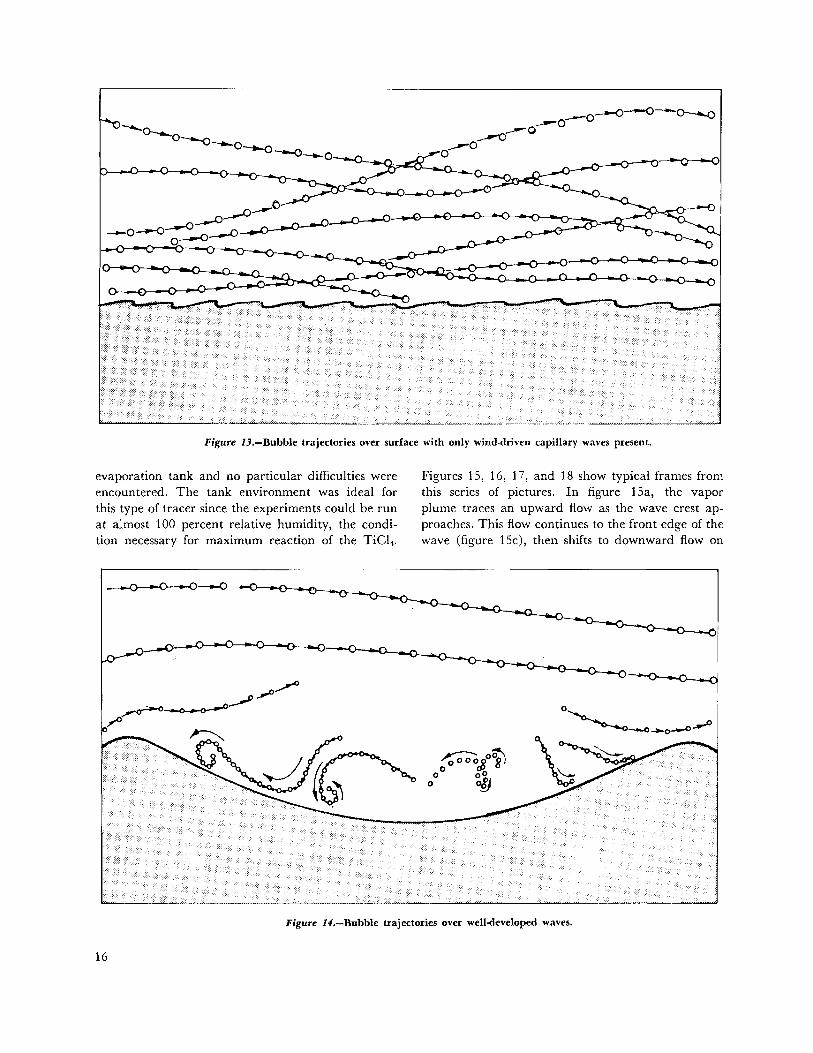
Figure H.-Bubble trajectories over surface with only wind-driven capillary waves present.

evaporation tank and no particular difficulties were encountered. The tank environment was ideal for this type of tracer since the experiments could be run at almost 100 percent relative humidity, the condi­tion necessary for maximum reaction of the TiCl4.

Figures 15, 16, 17, and 18 show typical frames from this series of pictures. In figure 15a, the vapor plume traces an upward flow as the wave crest ap­proaches. This flow continues to the front edge of the wave (figure 15c), then shifts to downward flow on

Figure U.-Bubble trajectories over well-developed waves.

16

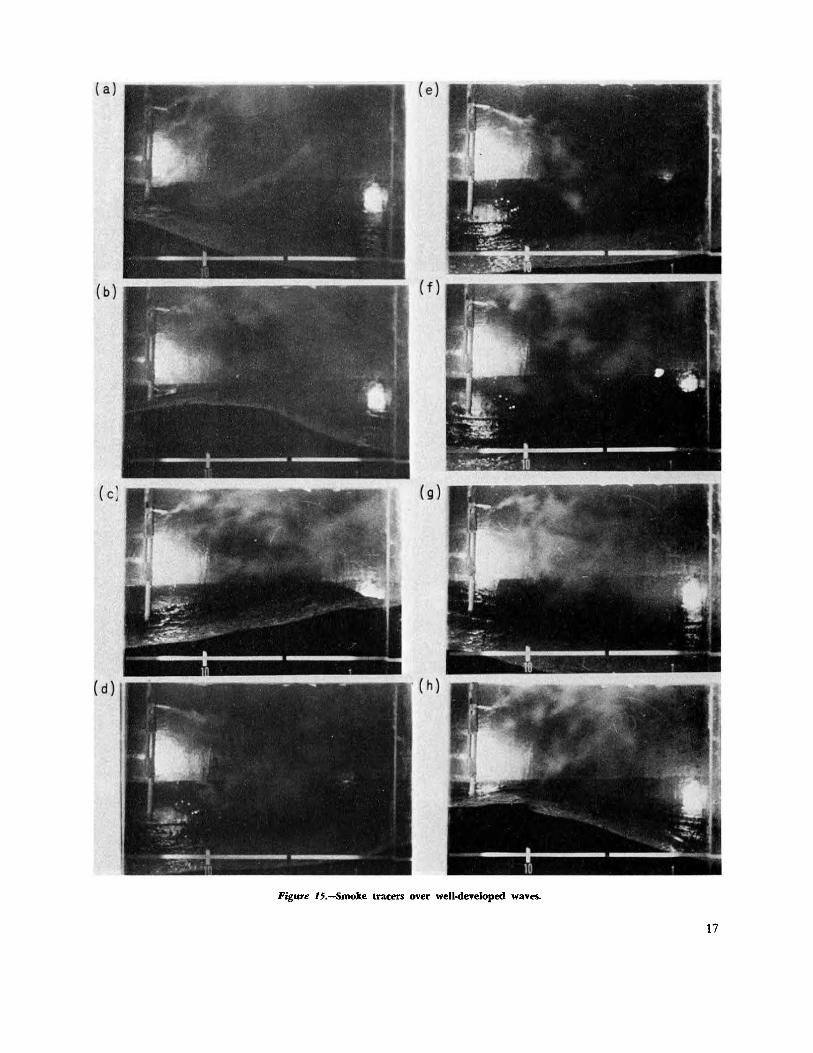
Figure H.-Smoke tracers over well-developed waves.

17

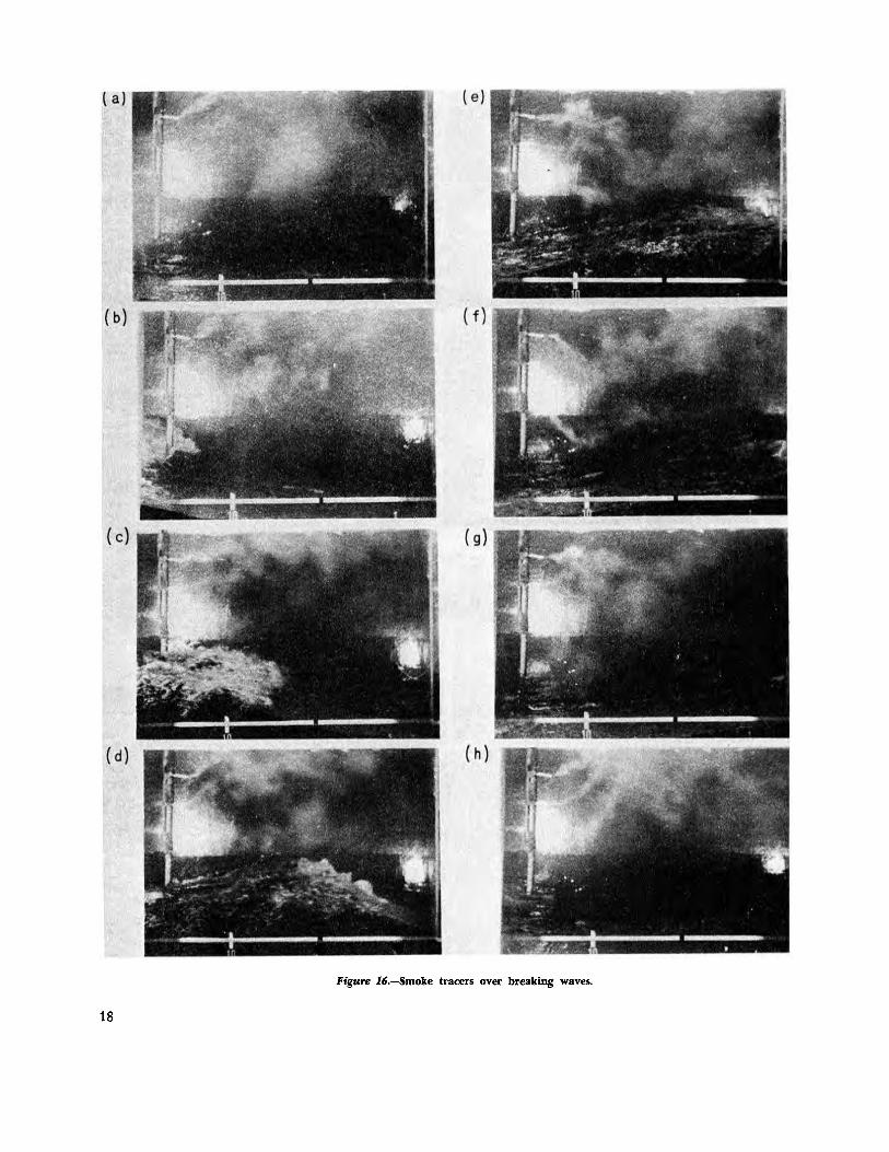
Figure 16.-Smoke tracers over breaking waves.

18

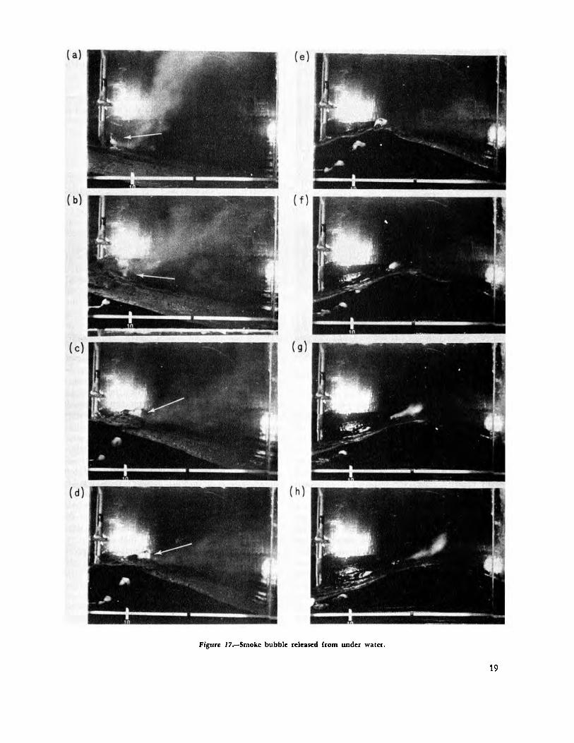
Figure 17.-Smokc bubble released from under water.

19

Fipre :11."'--Smoke tracers . showing reverse flow of air near surface ahead of approaching wave crest.

the upwind side of the crest. The trough region is characterized by rath~r random air motion at. this probe level (about 10 'inches above the undisturbed water surface}. The flow then shifts upward again ahead of the next wave crest (figures 15g-h). Figure 16 presents a similar series of frames but with a heavily breaking wave. The vapor tracer pattern is almost identical to that shown in figure 15.

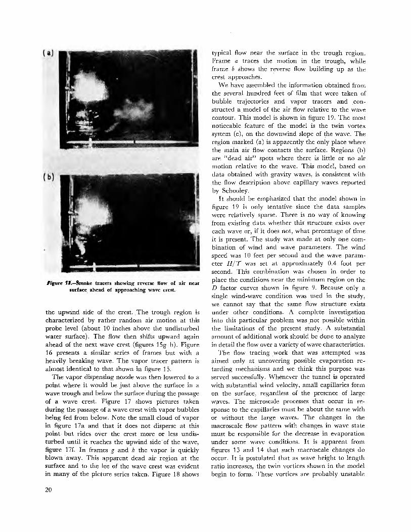
The vapor dispensing nozzle was then lowered to a point where it would be just above the surface in a wave trough and below the surface during the passage of a wave crest. Figure 17 shows pictures taken during the passage of a wave crest with vapor bubbles being fed from below. Note the small cloud of vapor in figure 17 a and . that it does not disperse at this point but rides over the crest more or less undis­turbed until it reaches the upwind side of the wave, figure 17L In frames g and h the vapor is quickly blown away. This apparent dead air region at the surface and to the lee of the wave crest was evident in many of the picture series taken. Figure 18 shows

20

typical flow near the surface in the trough region. Frame a traces the motion in the trough, while frame b shows the reverse flow building up as the crest approaches.

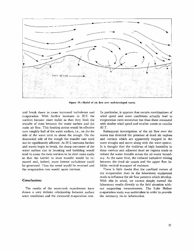
We have assembled the information obtained from the several hundred feet of film that were taken of bubble trajectories and vapor tracers and con­structed a model of the air flow relative to the wave contour. This model is shown in figure 19. The most noticeable feature of the model is the twin vortex system (c), ori the downwind slope of the wave. The region marked (a) is apparently the only place where the main air flow contacts the surface. Regions (b) are "dead air" spots where there is little or no air motion relative to the wave. This model, based on data obtained . with gravity waves, is consistent with the flow description above capillary waves reported by Schooley.

It should be emphasized that the model shown in figure 19 is only tentative since the data samples were relatively sparse. There is no way of knowing from existing data whether this structure exists over each wave or, if it does not, what percentage of time it is present. The study was made at only one com­bination of wind and wave parameters. The wind speed was 10 feet per second and the wave param­eter H/T was set at approximately 0.4 foot per second. This combination was chosen in order to place the conditions near the minimum region on the D factor curves shown in figure 9. Because only a single wind~wave condition was used in the study, we cannot say that the same flow structure exists under other conditions. A complete investigation into this particular problem was .riot possible within the limitations of the present study. A substantial amount of additionaJ work should be done to analyze in detail the flow over a variety of wave characteristics.

The ·flow tracing work that was attempted was aimed only at uncovering possible evaporation re­tarding mechanisms and we think this purpose was served successfully. Whenever the tunnel is operated with substantial wind velocity, small capillaries form on the surface, regardless of the presence of large waves. The microscale processes that occur in re­sponse to the capillaries must be about the same with or without the large waves. The changes in the macroscale flow pattern with changes in wave state must be responsible for the decrease in evaporation under some wave conditions. It is apparent from figures 13 and 14 that such macroscale changes do occur. It is postulated that aswave height to length ratio increases, the twin vortices shown in the model begin to form. These vortices are probably unstable

----

Figure 19.-Model of air flow over well-developed waves.

and break down to cause increased turbulence and evaporation. With further increases in H/ L the vortices become more ·stable so that they limit the transfer of mass between the water surface and the main air flow. This limiting action would be effective over roughly half of the water surface, i.e., on the lee side of the wave crest to about the trough. On the downwind side of the trough the transfer rate need not be significantly affected. As H/ L increases further and waves begin to break, the sharp curvature of the water surface due to breaking and bubbling would tend to cause the twin vortices to be shed more easily so that the barrier to mass transfer would be re­moved and, indeed, more intense turbulence could be generated. Thus the trend would be reversed and the evaporation rate would again increase.

Conclusions

The results of the wave-tank experiments have shown a very definite relationship between surface wave conditions and the measured evaporation rate.

In particular, it app~ars that certain combinations of wind speed and wave conditions actually lead to evaporation rat~s somewhat less than those meas~red with similar wind speed and smaller waves or. smaller H/T.

Subsequent investigation of the air flow over the waves has detected the presence of dead air regions and vortices which are apparently trapped in the wave troughs and move along with the wave system. It is thought that the build-up of high humidity in these vortices and adjacent dead air regions tends to reduce the water transfer across the air-water bound­ary. At the same time, the reduced turbulent mixing between the dead air spaces and the upper flow in.;. hibits vertical transport of moisture.

There is little doubt that the confined nature of the evaporation duct in the laboratory equipment tends to influence the air flow patterns which develop. With this in mind, we cannot simply extend the laboratory results directly to the field situation with­out supporting measurements. The· Lake Hefner evaporation study was undertaken in order.to provide the necessary tie-in information.

21

THE LAKE HEFNER EVAPORATION STUDY

In order to fulfill all objectives of the study as out­lined in the Introduction, it was necessary to extend the laboratory work into a full-scale field study. The Bureau of Reclamation had already organized an extensive evaporation study at Lake Hefner, Okla­homa, during the summer of 1966. Several different groups were to take part, including the Radio Meteorology Section of the Tropospheric Telecom­munications Laboratory of the Environmental Science Services Administration (ESSA). The ESSA group was scheduled to make evaporation measurements which appeared to ideally suit the needs of the CAL experiment. Thus, the CAL wave program was in­cluded in the 1966 study.

The program plan called for CAL to make wave measurements at two of the instrument stations at the lake and to use the meteorological records being taken by ESSA for evaporation computations. The instruments installed by ESSA were designed to make the measurements required for evaporation computations by the eddy flux method. The eddy flux equation for evaporation (Swinbank) 1s

E=pwW='PwW+pw'W'

where Pr& = vapor density W = vertical wind speed.

(21)

The primed symbols denote departures from the mean value. The averaging time must be long in compari­son to the longest period of fluctuation. The advective term 'Pw W is small near the surface where W::::: 0. Thus, we can equate the vapor flux (pw W) to the eddy flux (p,.,'W'). Instrumentation used for measuring Pw and W must respond to all fluctuations which contribute to the flux. However, very small-scale fluctuations will not contribute significantly to the vertical flux if the vapor density gradient is small. An indication of the magnitude of error to be expected in the flux estimate caused by slow response of instruments is given by Deacon. The eddy flux method was appro­priate for the CAL study because it gives a local evaporation rate, averaged over a relatively short time interval (10 minutes).

The eddy flux evaporation data were used to compute an eddy diffusion coefficient similar to the

22

one measured directly in the wave tank experiment. The Lake Hefner coefficients were computed using the equation

where E is the computed vapor flux, Pw' W' p = mean air density

(22)

ij.= saturation mixing ratio at the mean sur­face temperature

ij • = mean value of mixing ratio at level z. Coincident with the meteorological measurei'l;lents, time-height profiles of the lake surface level were recorded at each station. From these records, all re­quired wave information could be obtained. The wave data and calculated values of evaporation co­efficient were then used to study the relationship between evaporation and wave state.

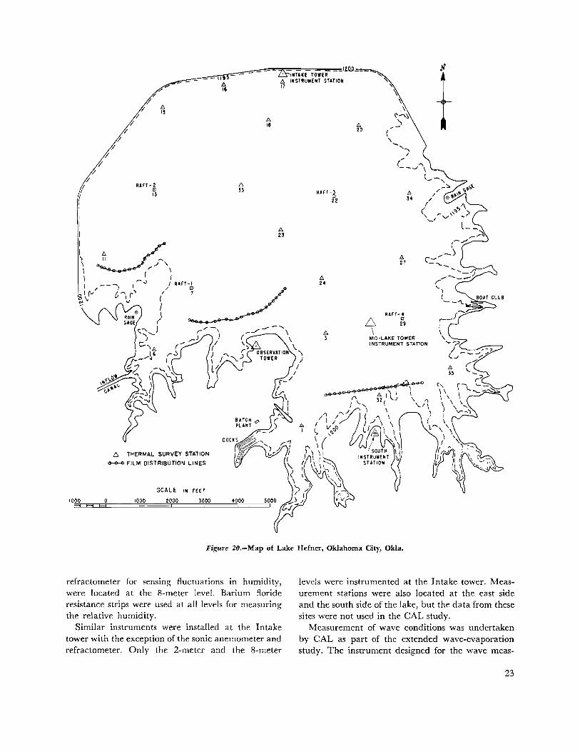
Figure 20 shows a map of Lake Hefner. The two instrument stations used for the CAL study were the Mid-lake tower station and the Intake tower station. The Mid-lake station is about two-thirds of a mile from the south shore; the Intake tower station is near the north shore with a fetch of about 2.5 miles for southerly winds. Southerly winds predominate in the area during late summer, and the instrument locations were planned to take advantage of this climatological feature.

Instrumentation at Lake Hefner

The instrumentation required for computation of evaporation rates was installed and operated by the ESSA group. The installations of prime importance to the CAL study were the Mid-lake tower and the Intake tower. The Mid-lake tower station was in­strumented at heights of 2, 8, and 16 meters. The absolute temperature measurement was made at 8 meters with temperature difference between 8 meters, the surface and the 2-meter level being sensed by thermocouples. The wind velocity measurements were made at all levels with propeller bivanes. The bivanes measured wind speed, azimuth angle IJ, and elevation angle tp. A sonic anemometer for meas­uring the vertical wind component, and a microwave

---- ___ 1£QD __ ' INTUE TOWER

4 INSTRUMENT STATION IT

1000 0

RAFT- 2 1!1 13

t:;. THERMAL SURVEY STATION

G-<H» FILM DISTRIBUTION LINES

SCALE IN FEET

1000 2000 3000

A II

RAFT-~

22

A 24

& 21

UFT-4

8 r, 4 \ 3 MIO·LAKE TOWER

INSTRUMENT STATION

Figure 20.-Map of Lake Hefner, Oklahoma City, Okla.

refractometer for sensing fluctuations in humidity, were located at the 8-meter level. Barium floride resistance strips were used at all levels for measuring the relative humidity.

Similar instruments were installed at the Intake tower with the exception of the sonic anemometer and refractometer. Only the 2-meter and the 8-meter

levels were instrumented at the Intake tower. Meas· urement stations were also located at the east side and the south side of the lake, but the data from these sites were not used in the CAL study.

Measurement of wave conditions was undertaken by CAL as part of the extended wave-evaporation study. The instrument designed for the wave meas-

23

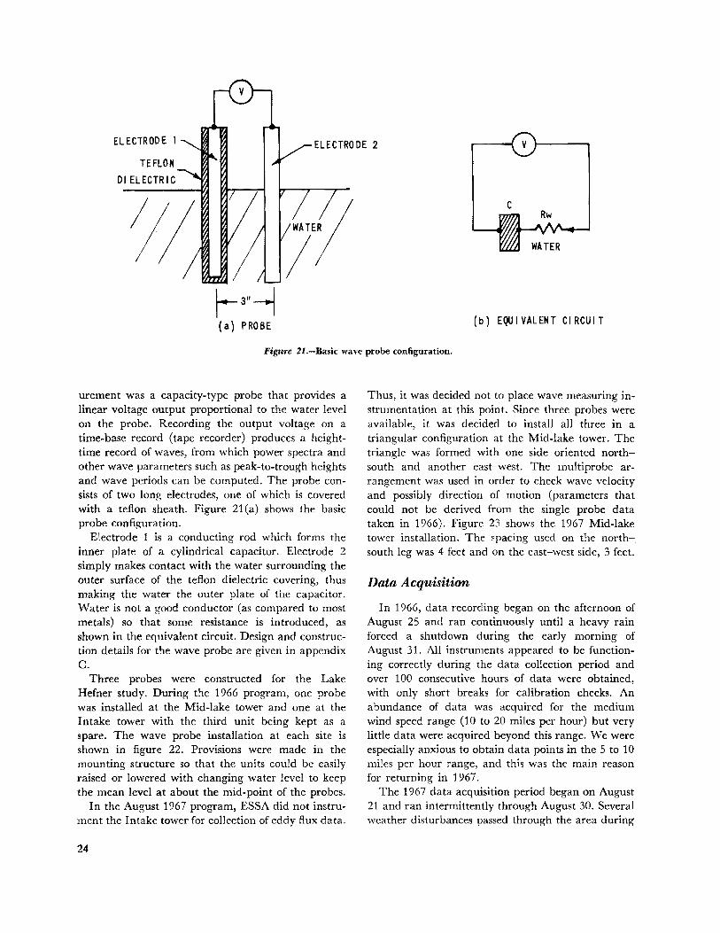
ELECTRODE 1

TEFLON

Dl ELECTRIC

ELECTRODE 2 v

c

r-3"~ (a) PROBE (b) EQUIVALENT CIRCUIT

Figure .21.-Basic wave probe configuration.

urement was a capacity-type probe that provides a linear voltage output proportional to the water level on the probe. Recording the output voltage on a time-base record (tape recorder) produces a height­time record of waves, from which power spectra and other wave parameters such as peak-to•trough heights and wave periods can be computed. The probe con­sists of two long electrodes, one of which is covered with a teflon sheath. Figure 21 (a) shows the basic probe configuration.

Electrode 1 is a conducting rod which forms the inner plate of a cylindrical capacitor. Electrode 2 simply makes contact with the water surrounding the outer surface of the teflon dielectric covering, thus making the water the outer plate of the capacitor. Water is not a good conductor (as compared to most metals) so that some resistance is introduced, as shown in the equivalent circuit. Design and construc­tion details for the wave probe are given in appendix c.

Three probes were constructed for the Lake Hefner study. During the 1966 program, one probe was installed at the Mid-lake tower and one at the Intake tower with the third unit being kept as a spare. The wave probe installation at each site is shown in figure 22. Provisions were made in the mounting structure so that the units could be easily raised or lowered with changing water level to keep the mean level at about the mid-point of the probes.

In the August 1967 program, ESSA did not instru­ment the Intake tower for collection of eddy flux data.

24

Thus, it was decided not to place wave measuring in­strumentation at this point. Since three probes were available, it was decided to install all three in a triangular configuration at the Mid-lake tower. The triangle was formed with one side oriented north­south and another east-west. The multiprobe ar­rangement was used in order to check wave velocity and possibly direction of motion (parameters that could not be derived from the single probe data taken in 1966). Figure 23 shows the 1967 Mid-lake tower installation. The spacing used on the north-. south leg was 4 feet and on the east-west side, 3 feet.

Data Acquisition

In 1966, data recording began on the afternoon of August 25 and ran continuously until a heavy rain forced a shutdown during the early morning of August 31. All instruments appeared to be function­ing correctly during the data collection period and over 100 consecutive hours of data were obtained, with only short breaks for calibration checks. An abundance of data was acquired for the medium wind speed range (10 to 20 miles per hour) but very little data were acquired beyond this range. We were especially anx,ious to obtain data points in the 5 to 10 miles per hour range, and this was the main reason for returning in 1967.

The 1967 data acquisition period began on August 21 and ran intermittently through August 30. Several weather disturbances passed through the area during

Figure 22.-Wave probe installation at Lake Hefner, 1966.

the period, temporarily shifth:i.g the wind out of the south. Nevertheless, several cases with southerly winds in the 5 to 10 miles per hour range were acquired and the CAL observations were terminated at the end of August, although the ESSA group re­mained with the hope of expanding the data sample.

Processing and Analysis of Lake Hefner Data

During the main data acquisition period in 1966, all data were recorded on ESSA magnetic tape re­corders, including the CAL wave probe outputs. For the sake of efficiency and cost it was agreed that CAL would use the data samples selected by ESSA, and that ESSA would compute the power spectra of the wave records and furnish them to us along with the meteorological parameters required to complete the analysis program outlined at the beginning of this section of the report.

In order to extend the data set, CAL personnel

visited ESSA and, using a Precision Instrument tape recorder, directly recorded 22 more samples (11 for each of the two sites).

During the 1967 field program the wave data were recorded . on a CAL recorder, along with the time code signal from the ESSA equipment. We then copied the required 1967 meteorological data along with the time code signal from ESSA tapes. The common time code on the two sets of tapes provided the means to time synchronize the two sets of data during the conversion to digital form for machine processing.

l. Initial data processing The raw data required for the analyses were:

(a) air temperature at 8 meters (b) il. T, surface to 8 meters (c) il.T, 2 meters to 8 meters (d) relative humidity at 2 meters (e) relative humidity at 8 meters (f) wind speed at 2 meters (g) elevation angle of 2-meter bivane (h) wind speed at 8 meters (i) elevation angle of 8-meter bivane (j) water surface level (wave probe).

Ten-minute sections were selected from the analog data records and converted to digital form using a sampling rate of 5 per second. This rate provided 3,000 data points per set. The digital data were then processed by computer. The outputs of the computer pro.gram were:

(a) mean surface temperature, T. (b) mean temperature at 2 meters, T2

(c) mean vapor density at 2 meters, l'tD2

(d) mean wind speed at 2 meters, v2 (e) mean vertical eddy flux of water vapor at 2

meters, Pw2 I W2 I

(f) mean temperature at 8 meters, T 8

(g) mean vapor density at 8 meters, PfDs

(h) mean wind speed at 8 meters, V8

(i) mean vertical flux 'of water vapor at 8 meters, f'tDs 1 W8 1

U) power spectrum of the water surface record [PwH(J)].

The wave power spectra were computed using the equal-time-spaced, discrete sample method of Black­man and Tukey. In addition to the wave power spectrum, the variance of the wave record . (u2wH) was also computed. By definition

(23)

and represents the total energy in the spectrum.

25

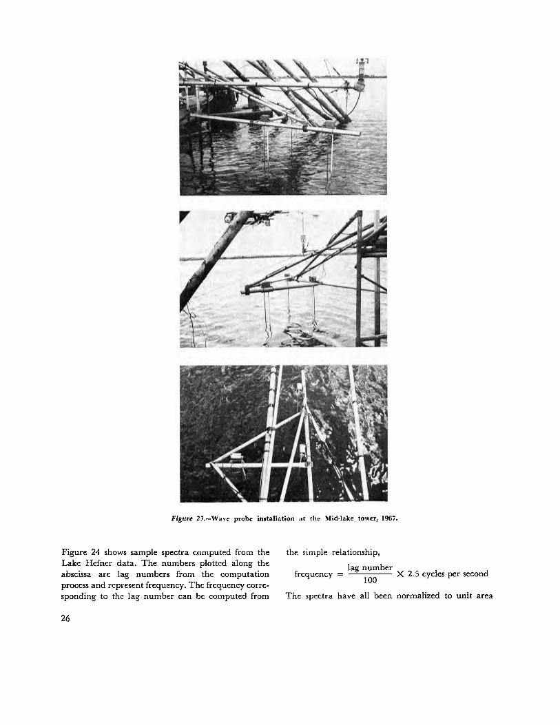
Figure 2J.-Wave probe installation at the Mid~lake tower, 1967.

Figure 24 shows sample spectra computed from the Lake Hefner data. The numbers plotted along the abscissa are lag numbers from the computation process and represent frequency. The frequency corre­sponding to the lag number can be computed from

26

the simple relationship,

lag number frequency = tOO X 2.5 cycles per second

The spectra have all been normalized to unit area

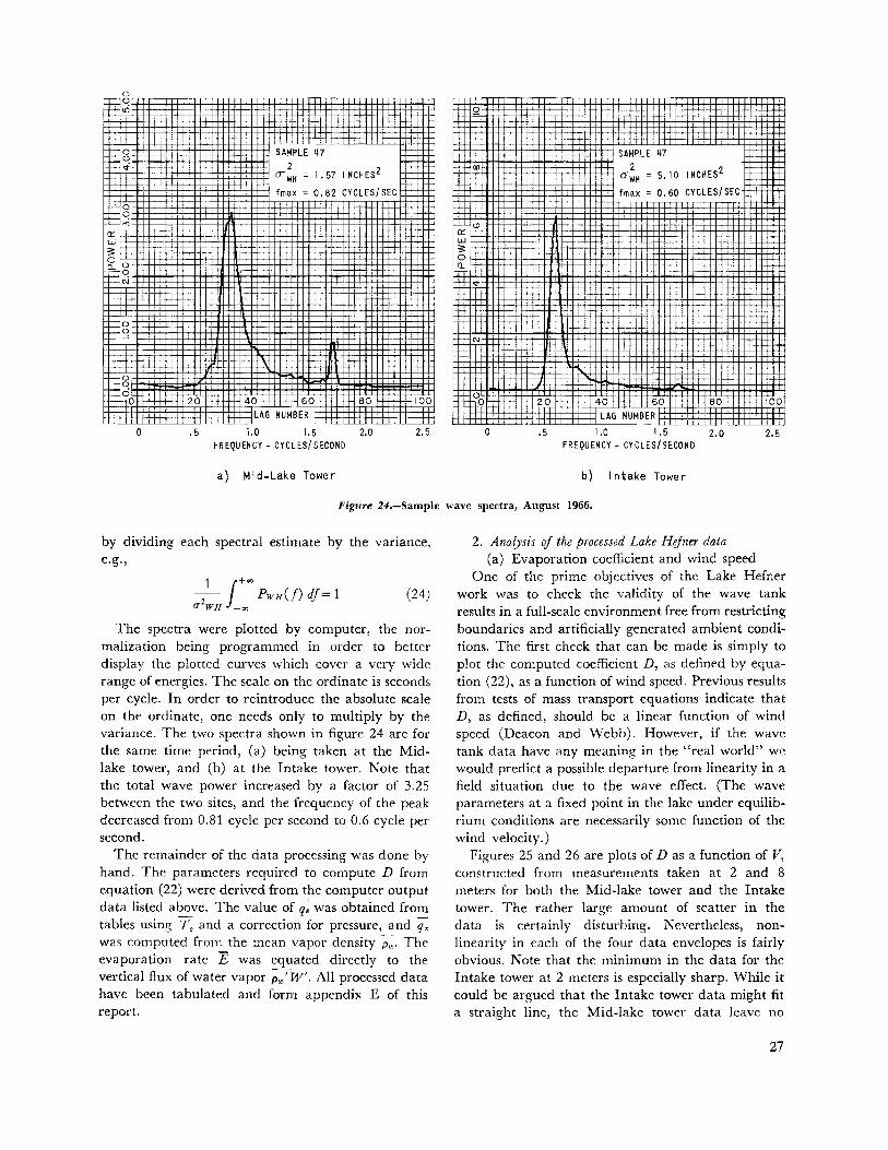
0 0 IIi 0

0 0

SAMPLE 117 SAMPLE 117 <i 2 2

~WH- 1.57 INCHES cr!H - 5. 10 INCHES2

fmax = 0.82 CYCLES/SEC fmax = 0. 60 CYCLES/ SEC 4+11-++t-H 0 C! ~

a:: w 3r: 00 0..0

N

0· g

N

0 0

20 40 60 eo 100 00 20 40 60 eo 100 0

0 LAG NUMBER LAG NUMBER

0 .5 1.0 1.5 2.0 2.5 0 .5 1.0 1.5 2.0 2.5 FREQUENCY- CYCLES/SECOND FREQUENCY- CYCLES/SECOND

a) Mid-Lake Tower b) Intake Tower

Figure 24.-Sample wave spectra, August 1966.

by dividing each spectral estimate by the variance, e.g.,

1 /+"' - 2 - PwH(J) dj = 1 f1 WH -oo

(24)

The spectra were plotted by computer, the nor­malization being programmed in order to better display the plotted curves which cover a very wide range of energies. The scale on the ordinate is seconds per cycle. In order to reintroduce the absolute scale on the ordinate, one needs only to multiply by the variance. The two spectra shown in figure 24 are for the same time period, (a) being taken at the Mid­lake tower, and (b) at the Intake tower. Note that the total wave power increased by a factor of 3.25 between the two sites, and the frequency of the peak decreased from 0.81 cycle per second to 0.6 cycle per second.

The remainder of the data processing was done by hand. The parameters required to compute D from equation (22) were derived from the computer output data listed above. The value of q. was obtained from tables using T. and a correction for pressure, and q. was computed from the mean vapor density Pw· The evaporation rate E was equated directly to the vertical flux of water vapor Pw'W'. All processed data have been tabulated and form appendix E of this report.

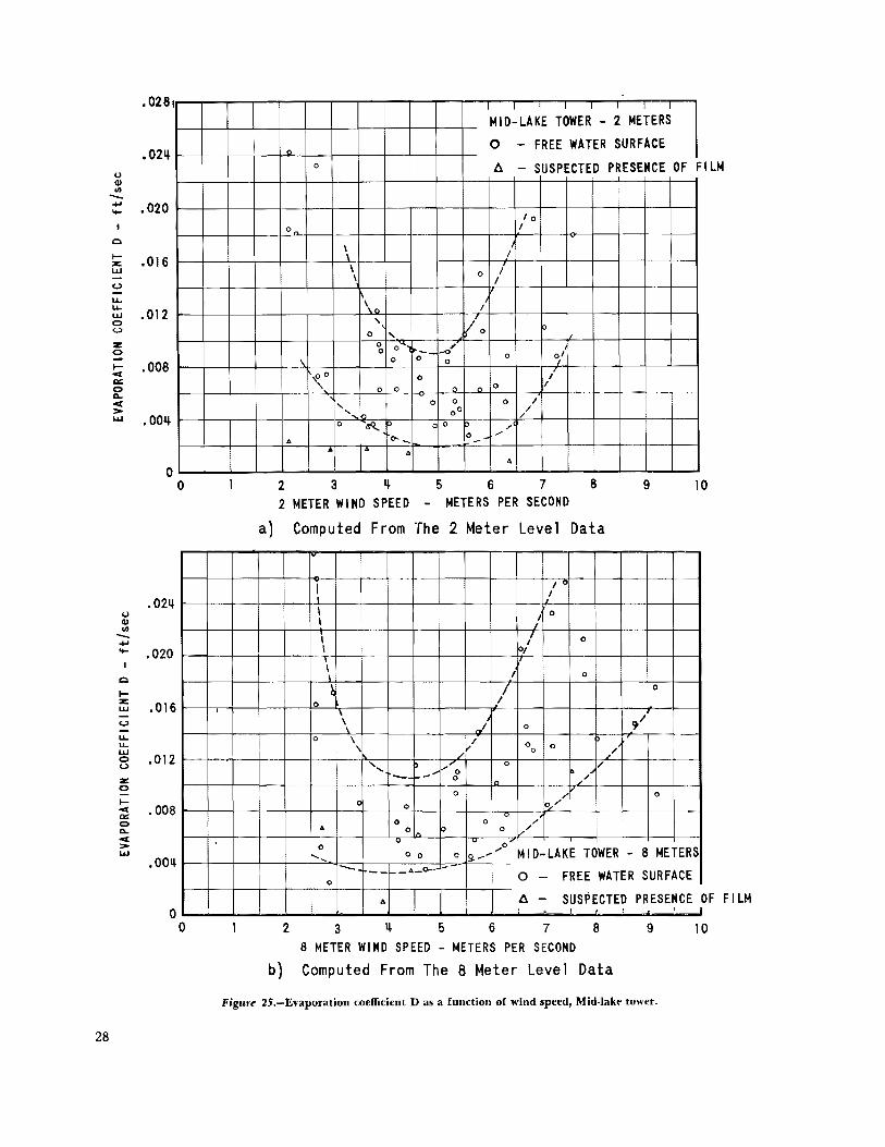
2. Anarysis of the processed Lake Hefner data (a) Evaporation coefficient and wind speed

One of the prime objectives of the Lake Hefner work was to check the validity of the wave tank results in a full-scale environment free from restricting boundaries and artificially generated ambient condi­tions. The first check that can be made is simply to plot the computed coefficient D, as defined by equa­tion (22), as a function of wind speed. Previous results from tests of mass transport equations indicate that D, as defined, should be a linear function of wind speed (Deacon and Webb). However, if the wave tank data have any meaning in the "real world" we would predict a possible departure from linearity in a field situation due to the wave effect. (The wave parameters at a fixed point in the lake under equilib­rium conditions are necessarily some function of the wind velocity.)

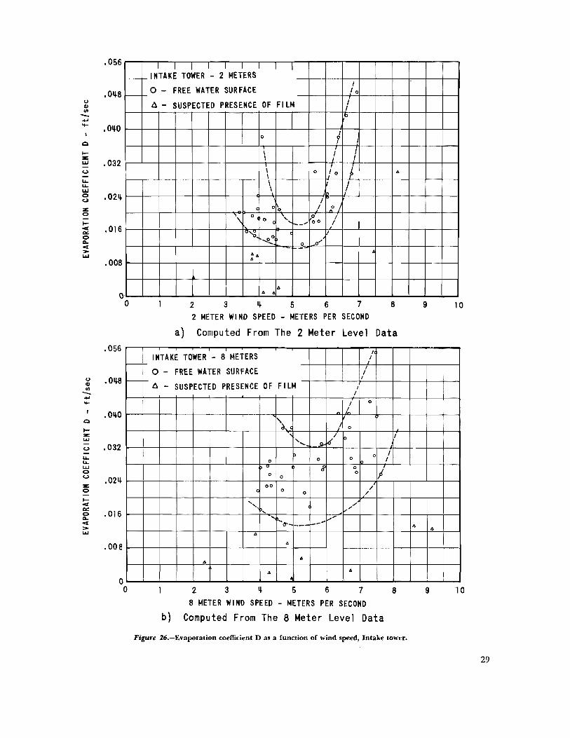
Figures 25 and 26 are plots of D as a function of V, constructed from measurements taken at 2 and 8 meters for both the Mid-lake tower and the Intake tower. The rather large amount of scatter in the data is certainly disturbing. Nevertheless, non­linearity in each of the four data envelopes is fairly obvious. Note that the minimum in the data for the Intake tower at 2 meters is especially sharp. While it could be argued that the Intake tower data might fit a straight line, the Mid-lake tower data leave no

27

u CD ., -+' ....

Q

1-z: UJ

(,)

u.. u.. UJ 0 (,)

z: 0

1-• a:: 0 a. • > UJ

u CD ., -+' ....

Q

1-z: UJ

(,)

u.. u.. UJ 0 (,)

*' 0

1-• a:: 0 a. .. > UJ

28

.028 I

.02"

.020

.016

.012

.008

.00~

0 0

.02~

.020

.016

.012

.008

• 00~

0 0

-I I I I T I L I

MID-LAKE TOWER - 2 METERS

" 0 - FREE WATER SURFACE

0 1:1 - SUSPECTED PRESENCE OF F ILM

lo 0 I

\ I

\ / \ o I

'-\o I

' v'o 0 0 ' ~ 0 ... ,

0--

_ .. .. 0 0 ~I 0

~0 0 I 0 0 n " 0

I

' 0 0 0 I

' 00 / /

0 4Q,. oo ~ "' o-_ 0-~ "' ... ... I" A 4

2 3 ~ 5 6 7 8 9 10 2 METER WIND SPEED - METERS PER SECOND

a) Computed From The 2 Meter Level Data

\ I o

I

I I o I i I o/

0

\ l

\ I 0

~ / 0

D •'

\ \ ,../ 0 '.I

0 \ / 0 0 0 ,/

' .... "'"o " ,/ - _ ...

0 ... ..-· 0

p ........... 0 c 0

u 0 0 / ... 0 0 0 I/''

0 v -v ,.,o ...... 0 0 0 ~ .... MID-LAKE TOWER - 8 METERS -- ----A ..,o-~

0 0 - FREE WATER SURFACE

... 1:1 - SUSPECTED PRESE~CE p F FILM

2 3 5 6 7 8 9 10 8 METER WIND SPEED - METERS PER SECOND

b) Computed From The 8 Meter Level Data

Figure 2J'.-Evaporation coefficient D as a function of wind speed, Mid·lake tower.

C) Ql 0 -.... .... c 1-:z: 1.1.1

c.> u.. u.. 1.1.1 0 c.> :z: 0

1-oC a&: 0 D. oC > 1.1.1

u Ql ., -.... .... c 1-:z: 1.1.1

c.> u.. u.. 1.1.1 0 c.>

:z: 0

1-oC Q: 0 D. oC > 1.1.1

.056

-.0118 -

.OliO

.032

.0211

.016

• 008

0 0

I I I I I I I I I ~INTAKE TOWER- 2 METERS

0 - FREE WATER SURFACE I lo

1-

~- SUSPECTED PRESENCE Of Fl~ I I

,10

0 I ?

I I I I

\ i 0 fo t .. \ I

I c 00 I o I

\ 0 ', 0 I 0 (

__ ,. oo I

"'0, ..J!o o" .... 0

.... .. ~

.. .. 2 3 5 6 7 8

2 METER WIND SPEED - METERS PER SECOND

a} Computed From The 2 Meter Level Data .056

INTAKE TOWER - 8 METERS I I

-r- I 0 - FREE WATER SURFACE I I , oqs - - ~ - SUSPECTED PRESENCE Of FILM I

.OliO

• 032

.021J

.016

.008

0 0

I

I 0

I~

\ I o

~I f> .... ,g,. .....

~ 0 0 0 0

... 8 0

I 0 0 0

0 oo 0 /

0 /

'-.. , I' 1--' .,

~-----',..~ --- f-_ ....

.. A

A A

A ..

2 3 5 6 7 8 METER WIND SPEED - METERS PER SECOND

b) Computed From The 8 Meter Level Data

I

I I

8

Figuf'e 26.-Evaporation coefficient D as a function of wind speed, Intake tower.

9 10

A ..

9 10

29

7

4,.~"'" 6

I .1 I I I I J ,.._4,.)-~V o 1--_VARIANCE OF WAVE HEIGHT

AS A FUNCTION OF 2 METER 0 ~ /

5 N

r-- -WIND SPEED r lo /

I In G)

.c:: CJ II-c

z: • 3 LIJ (,) z

I ~~-'\~~

I 7 ~ --.;):_~

~I ~ / ..,,~,

v l/"'. .,.

/ c 0::: c 2 >

j y ol ..... v

/~ v i

/ .J ~

0 0 2 3 II- 5 6 7 8 9

2 METER WIND SPEED - METERS PER SECOND

Figure 27.-Total wave energy as a function of the 2-meter wind speed.

doubt about the existence of a minimum in D for wind speeds of 4 to 5 meters per second.

(b) Wave data analysis In order to make a comparison between laboratory

results and Lake Hefner data, the Lake Hefner wind­wave relationships are required. Twenty-four wave power spectra were computed, representing the full range of wind speeds encountered during the field studies. The spectra were all strongly peaked with little wave energy outside the significant wave fre­quency. The peak frequency could be read very easily from each spectrum. This frequency was deter­mined and converted to wave period.

Along with wave spectra, the variance or total wave energy was also computed. By taking the square root of the variance we obtain the standard deviation of the wave record. Since the spectra indi­cate very strongly monochromatic waves, and since the waves are nearly sinusoidal in shape, it is not un­realistic to equate the measured standard deviation to the rms value of an equivalent sine wave. The peak­to-trough wave height may then be estimated using the expression:

H=2V2uwn (25)

30

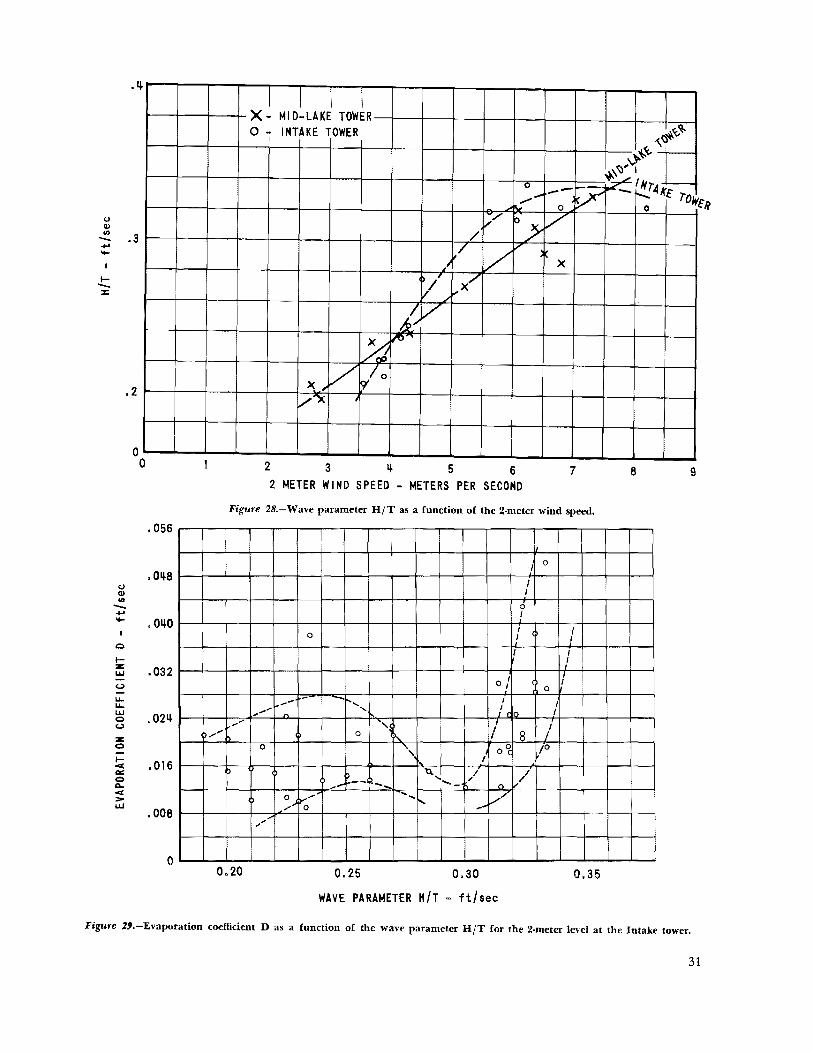
The wave spectra and the variance thus provided the necessary information for computing the wave param­eter H/ T. Figure 27 presents a plot of wave energy (u 2wn) as a function of 2-meter wind speed for both the Mid-lake tower and the Intake tower. Note that at a wind speed of 7 to 8 meters per second the wave energy at the Mid-lake tower is still increasing at a near constant rate, while the wave energy at the Intake tower is beginning to reach a maximum. Figure 28 shows the wave parameters or wave height­to-period ratio (H/ T) for both sites. Again the Mid­lake tower curve is linear, while that for the Intake tower has a parabolic shape due to the amplitude limiting occurring over the much longer fetch.

Since the wave parameter versus wind speed curve is linear for the Mid-lake tower, a plot of the coeffi­cient D versus H/ T would show a distribution similar to those in figures 25 and 26. However, this is not necessarily true for the Intake tower. Figure 29 shows a plot of D as a function of H/Tfor the 2-meter level at the Intake tower. Although the (H/T, V) rela­tionship is nonlinear, this has not appreciably altered the D coefficient envelope. The gross departure from linearity and the minimum (at H/T=0.3) remains as in the wind-dependent curves.

u Q)

.~

-! .3 .... .... .... -:z::

u Q) Cl)

.2

0 0

-.... .... I

Q

.... z: L&.l

(,)

u.. u.. L&.l 0 (,)

z: 0

.... cc co: 0 A.. cc > L&.l

.056

.0~8

.0~

.032

. on

.016

.008

0

I I I I X- Ml D-LAKE TOWER

~~'+-0 - INTAKE TOWER ~'\:

~,t~ .L +' 0 --~- ~.1llr4k. ..,... .... ~" "'; E TOtfJ ... 0

~/ / ~> v

/ vv L~ X

/ l/ ~>("

1: v A

jt'O'

X v ~lo v~ J

2 3 ~ 5 6 7 8 9 2 METER WIND SPEED - METERS PER SECOND

FigtWe 28.-Wave parameter H/T as a function of the 2·meter wind speed.

! 0

I I

0 I

I I 0 I I

I I

I 0 I ( I I 0 - r-... I I ....... I ...... ... lo I ... _n. ... ' l 8 / , ... 0

·~ I 0 ',

I o? fO

-- 'a., ..... _ / n L,/ ....... -..

0 IY ... r ........ t' .... v"" ....... 0

..... ..-·

0.20 0.25 0.30 0.35

WAVE PARAMETER H/T - ft/sec

Figure 2'.-Evaporation coefficient D as a function of the wave parameter H/T for the 2·meter level at the Intake tower.

31

COMPARISON OF THE LABORATORY AND FIELD RESULTS

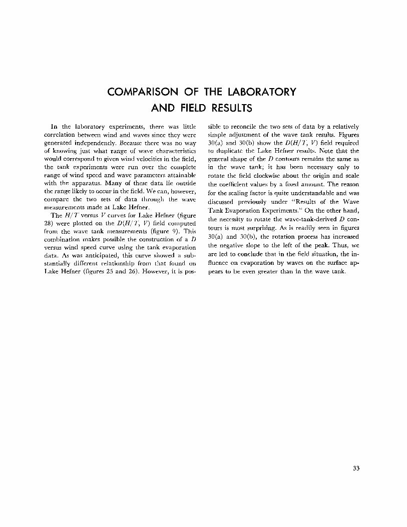
In the laboratory experiments, there was little correlation between wind and waves since they were generated independently. Because there was no way of knowing just what range of wave characteristics would correspond to given wind velocities in the field, the tank experiments were run over the complete range of wind speed and wave parameters attainable with the apparatus. Many of these data lie outside the range likely to occur in the field. We can, however, compare the two sets of data through the wave measurements made at Lake Hefner.

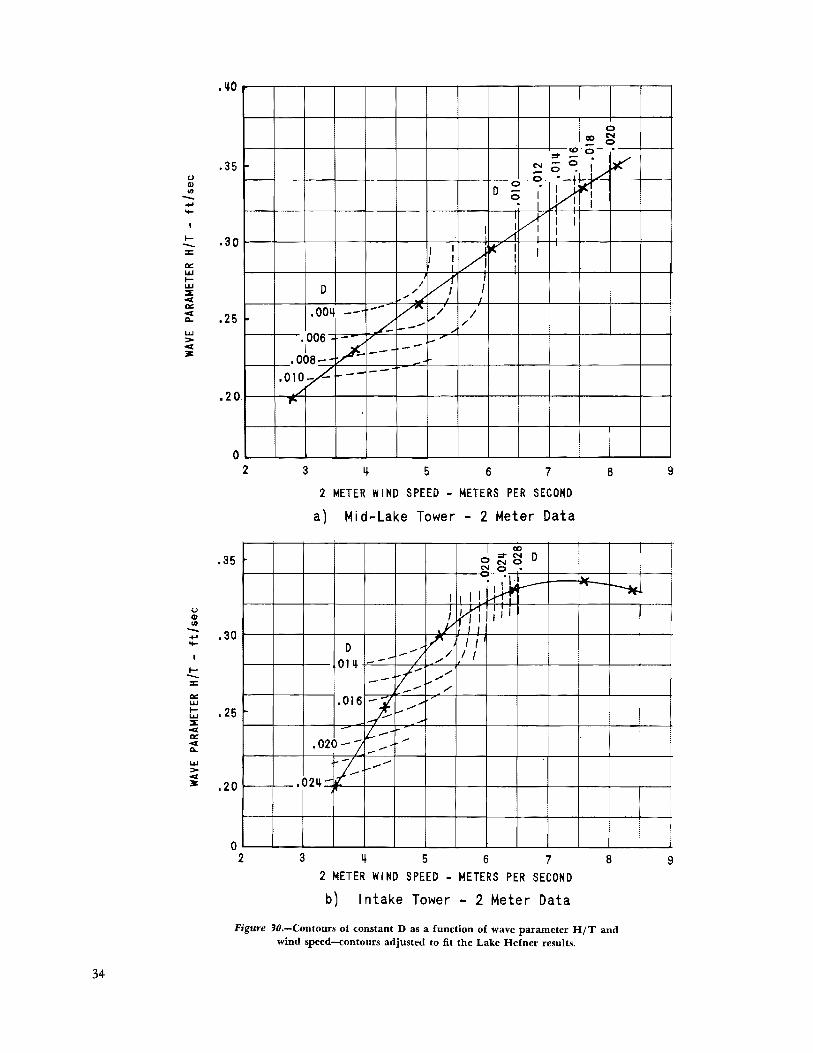
The H/T versus V curves for Lake Hefner (figure 28) were plotted on the D(H/T, V) field computed from the wave tank measurements (figure 9). This combination makes possible the construction of a D versus wind speed curve using the tank evaporation data. As was anticipated, this curve showed a sub­stantially different relationship from that found on Lake Hefner (figures 25 and 26). However, it is pos-

sible to reconcile the two sets of data by a relatively simple adjustment of the wave tank results. Figures 30(a) and 30(b) show the D(H/T, V) field required to duplicate the Lake Hefner results. Note that the general shape of the D contours remains the same as in the wave tank; it has been necessary only to rotate the field clockwise about the origin and scale the coefficient values by a fixed amount. The reason for the scaling factor is quite understandable and was discussed previously under "Results of the Wave Tank Evaporation Experiments." On the other hand, the necessity to rotate the wave-tank-derived D con­tours is most surprising. As is readily seen in figures 30(a) and 30(b), the rotation process has increased the negative slope to the left of the peak. Thus, we are led to conclude that in the field situation, the in­fluence on evaporation by waves on the surface ap­pears to be even greater than in the wave tank.

33

u II) ~ -.... ....

1--:c a.:: 1.1.1 1-1.1.1 ::E c a.:: c A-

1.1.1 > c 31=

u II) ~ -.... ....

1--:c a.:: 1.1.1 1-1.1.1 ::E c a.:: c A-

1.1.1 > c 31=

34

.35 1-

.so

.25

1[/f' I I I A i I

I I j~ I I I !/1 !

D

• ooq -- _... V"' / 1 L .... --k /

.006 ~ I I ,r --- --

~-+-'008~-~-~~~+-~~~~-+--4---+--4---+--~--+-_, .010;7 ----

.20 j

OL--L--L--L--~~--~~--~~--~~--~--~~

2

.35

.30

.25

.20

0 2

3 q 5 6 7

2 METER WIND SPEED - METERS PER SECOND

a) Mid-Lake Tower - 2 Meter Data

l::r~o ONO N 0 •

,,,,;w..-7 m,r,, .v i j

D ,..-; V' I / 1 __ ... / I I OJq ....

~= / -- !-- ..... /

.016 17-~---- .... ·'

...... - lL-. 020-j ... --~ !-- ..........

.02!l-

3 q 5 6 7 2 METER WIND SPEED - METERS PER SECOND

b) Intake Tower - 2 Meter Data

8

...... ~

8

Figure JO.-Contours of constant D as a function of wave parameter H/T and wind speed-contours adjusted to fit the Lake Hefner results.

9

9

EVAPORATION ESTIMATES AND WAVES

Although every attempt was made to make the Lake Hefner study as quantitative as possible, there was considerable scatter in the processed data and the overall evaporation estimates were somewhat lower than existing water budget information would have predicted. The reasons for the apparent inac­curacies in the evaporation estimates are very likely due to departure from the ideal conditions assumed in developing the eddy flux theory. For example, neglecting the advective term 'Pw W by assuming W = 0, does not necessarily hold. In fact, the mean vertical wind was never zero in any of the processed samples, although this could have been due to small errors in calibration of the bivanes. There was also some evidence that the humidity and wind measuring instruments did not have fast enough response times to follow all the significant eddy scales. Comparison of the measured vapor fluxes from the Mid-lake tower and the Intake tower tend to suggest that the Mid­lake instruments were located on the outer fringe of the vapor blanket. Significantly lower values of the vapor density variance at the Mid-lake tower leads us to this conclusion. The apparent thinness of the vapor blanket at the Mid-lake tower (if this is truly the case) may be due to the reduction in vertical transport of water vapor caused by the waves on the water surface.

While the absolute measurements of evaporation may be somewhat in error, changes in the measured parameters relative to some chosen base value are thought to be more reliable. Thus, we have chosen to use the shape of the measured curve of mass transfer coefficient as a function of wind speed (and the de­pendent wave parameters), and to adjust the absolute magnitude using the many available water-budget­derived values.

Marciano and Harbeck derived two empirical equations of best fit for Lake Hefner, using slightly different data for each. These are,

E= 6.25 X 10-4Vs(eo-es) (26)

and E= 6.47 X 10-4V,.(e.o-e.,) (27)

where E= evaporation in centimeters per 3 hours Vs = wind speed in knots at 8 meters , !t.e = vapor pressure difference in millibars.

Linsley, Kohler, and Paulhus also derived two equa­tions from slightly different data inputs,

(28)

and

(29)

where E= evaporation in inches per day V4= wind speed in miles per day at 4 meters !t.e = vapor pressure difference in inches of

mercury.

During 1965, Oklahoma State University, working for the Bureau of Reclamation, did yet another survey of Lake Hefner. Fry reports two more estimates of the mass transport coefficients, using hoth water budget and energy budget methods. The water budget form is:

where E= evaporation in centimeters per day V2 = wind speed in kilometers per day at 2

meters !t.e = vapor pressure difference in millibars.

All the above equations report a different value of N because they each use different units. Since none of the above forms match the units used in the CAL study, we have chosen to transform these equations to fit our units. The equations reduce to the following (in the order presented):

E=5.38 X10-5Vs(q.-qs)

E= 5.56X10-5V.,(q,-q.,) 1\

E= 6.65X1Q-5V4(q.-q2)

E= 5.92X 1Q-6V4(q.-q2)

E= 6.17X10-5V2(q,-q2)

35

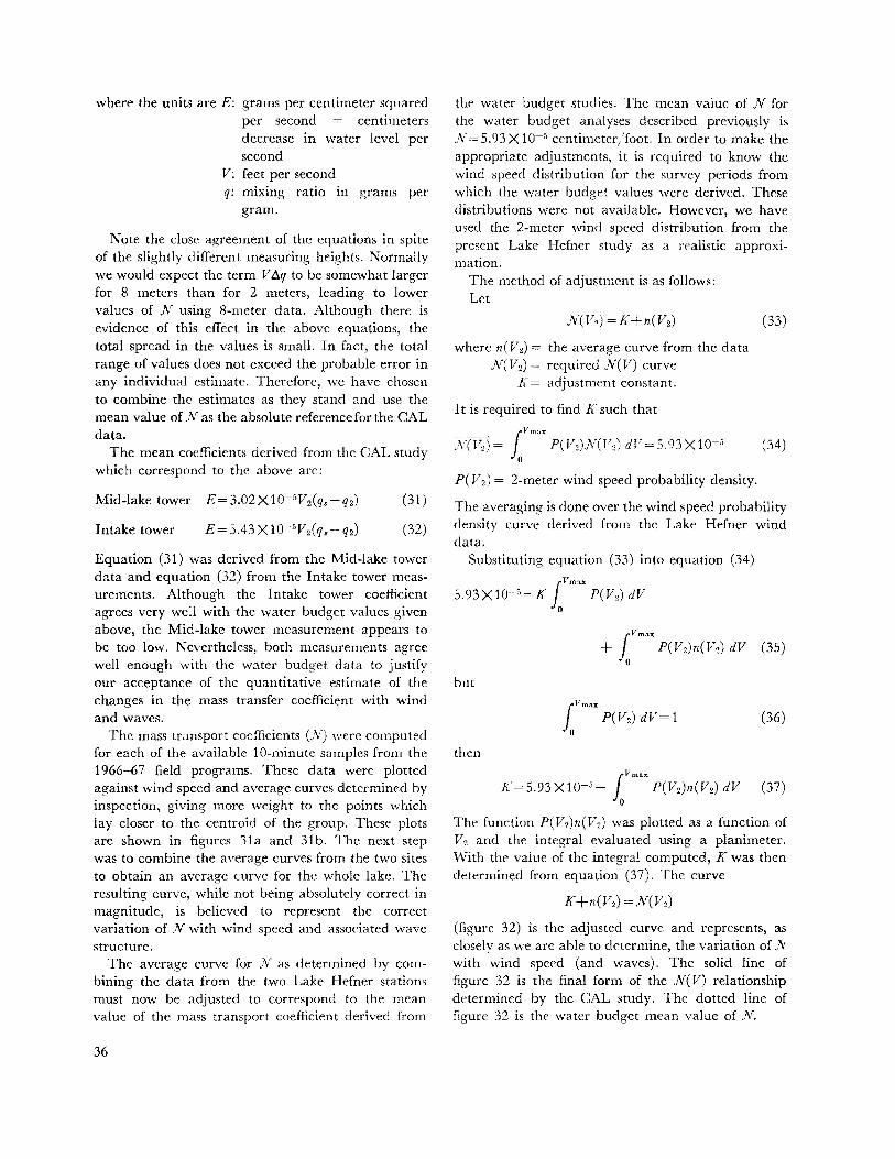
where the units are E: grams per centimeter squared per second = centimeters decrease in water level per second

V: feet per second q: mixing ratio in grams per

gram.

Note the close agreement of the equations in spite of the slightly different measuring heights. Normally we would expect the term V.1q to be somewhat larger for 8 meters than for 2 meters, leading to lower values of N using 8-meter data. Although there is evidence of this effect in the above equations, the total spread in the values is small. In fact, the total range of values does not exceed the probable error in any individual estimate. Therefore, we have chosen to combine the estimates as they stand and use the mean value of N as the absolute referenceforthe CAL data.

The mean coefficients derived from the CAL study which correspond to the above are:

Mid-lake tower E=3.02X10-6V2(q,-q2) (31)

Intake tower (32)

Equation (31) was derived from the Mid-lake tower data and equation (32) from the Intake tower meas­urements. Although the Intake tower coefficient agrees very well with the water budget values given above, the Mid-lake tower measurement appears to be too low. Nevertheless, both measurements agree well enough with the water budget data to justify our acceptance of the quantitative estimate of the changes in the mass transfer coefficient with wind and waves.

The mass transport coefficients (N) were computed for each of the available 1 0-minute samples from the 1966-67 field programs. These data were plotted against wind speed and average curves determined by inspection, giving more weight to the points which lay closer to the centroid of the group. These plots are shown in figures 31a and 31 b. The next step was to combine the average curves from the two sites to obtain an average curve for the whole lake. The resulting curve, while not being absolutely correct in magnitude, is believed to represent the correct variation of N with wind speed and associated wave structure.

The average curve for N as determined by com­bining the data from the two Lake Hefner stations must now be adjusted to correspond to the mean value of the mass transport coefficient derived from

36

the water budget studies. The mean value of N for the water budget analyses described previously is N=5.93X10-5 centimeter/foot. In order to make the appropriate adjustments, it is required to know the wind speed distribution for the survey periods from which the water budget values were derived. These distributions were not available. However, we have used the 2-meter wind speed distribution from the present Lake Hefner study as a realistic approxi­mation.

The method of adjustment is as follows: Let

where n(V2) = the average curve from the data N(V2) = required N(V) curve

K = adjustment constant.

It is required to find K such that

N(V2)= ~Vmax P(Vz)N(V2) dV=5.93X10-5

0

P(Vz) = 2-meter wind speed probability density.

(33)

(34)

The averaging is done over the wind speed probability density curve derived from the Lake Hefner wind data.

Substituting equation (33) into equation (34)

5.93X10-5 =K ~Vmax P(Vz) dV 0

but

then

1Vmax

P(V2) dV=1 0

K=5.93Xto-•- ~vmax P(V2)n(Vz) dV 0

(36)

(37)

The function P(Vz)n(V2) was plotted as a function of v2 and the integral evaluated using a planimeter. With the value of the integral computed, K was then determined from equation (37). The curve

(figure 32) is the adjusted curve and represents, as closely as we are able to determine, the variation of Jv with wind speed (and waves). The solid line of figure 32 is the final form of the N(V) relationship determined by the CAL study. The dotted line of figure 32 is the water budget mean value of N.

.... .... -

10

8

5 6

)(

z:

.... .... -e CJ

10

0

)(

z:

2

0 ~

1~

12

10

8

6

~

2

0 ~

6

6

- -...... /

' / -- 0 ~ v 0 / -o- .... 0" 0 /

............. 0 0 ~ v "" ,." ~ ... ib- 0 /

0 "' ......... 0 .... -c: ;0 v 0 - -:.IQ_

0 r< o.lt -- ..... 0 p r-;;-h- " ~ 1--ro--

8 1 0 12 1 ~ 16 18 20 22

2 METER WIND SPEED - ft/sec

a) Mid-Lake Tower - 2 Meter Data.

\0

\ / I J v j

.....- - .... , 1\ 1/ i/ ,."' ', 0 \ I 0

/' 0 ,, /

I' o"c< \ ~I' i/ v ~' 0

,..--r--. "'\ '\['..... ,...,.,., v _{o / 0 0 nf

_...V "" " 't, --"' v ..... ~ 0

v ~ 0 - - v

o,l OQ !---... / - v --

8 10 12 1 ~ 16 18 20 22

2 METER WIND SPEED - ft/sec

b) Intake Tower - 2 Meter Data

Figure Jl.-Mass transfer coefficient N as a function of wind speed.

The N(V) curve presented in figure 32 is the "instantaneous" value of N for the equilibrium wind speed V. The term "instantaneous" refers to the length of time the wind speed, and other parameters required in the evaporation estimate, remain rela-

tively constant. The curve was developed using mean measurements over 10-minute time intervals.

It should be emphasized that the variable N rela­tionship shown in figure 32 should not be used with long-period averaged inputs. For example, if the wind

37

10

9

8

7 .... ~ - 6 E

"' "" 5

0

I / ,...,- - v

/ "" /

"" / /

H = 5.93 X 10-5

"" -....... / ~ - -----

/ X ~ z:

3

2

0

6 8 10 12 16 18 20 22

MEAN WIND SPEED AT 2 METERS - ft/sec

Figure 12.-Mass transfer coefficient N as a function of wind speed-curve adjusted to fit water budget data.

speed were constant at 13 feet per second for 12 hours and then increased to 21 feet per second for 12 hours, the mean wind for the 24-hour period would be 17 feet per second. If we now go to the curve with this 24-hour mean wind, we find that Nis 4.3X10-5,

a low and incorrect value. If, on the other hand, we recognize the true meaning of the curve, we must determine N for 13 feet per second and again for 21 feet per second. In both cases this value is about 6.0X10-5, making the correct value for the 24-hour period 6.0X10-5•

If the curve is correctly applied, it should lead to more accurate estimates of evaporation over long time periods where wind speeds have remained rela­tively constant during certain portions of the period. For example, if during a one-week survey period, the

38

wind speed remained near 17 feet per second for a large percentage of the time, use of the water-budget­derived coefficient would lead to an overestimate of the actual evaporation. Figure 32 shows that the true evaporation would be approximately 30 percent less than that given by the constant-N relationship. To successfully make use of this new relationship for long survey periods it will generally be necessary to compute the evaporation for short periods (possibly one hour) and sum the' results. For very long periods, however, where one can expect the wind speed distribution to approach the one used in the analysis, the new N(V) curve will not improve the estimate over the N = constant approach. In fact, the two methods should give the same result since the N(V) curve was adjusted to satisfy just this requirement.

CONCLUSIONS AND RECOMMENDATIONS

Despite certain difficulties with techniques and instrumentation, some very useful results have been obtained. The wave tank measurements showed that waves apparently modify the air flow over the surface in such a way that turbulent transport mechanisms can be suppressed. Follow-up experiments conducted in the field tend to support the tank measurements, and in fact show that the evaporation retarding mechanism appears to be even more effective in the field.

The results of both the laboratory and the field studies tend to confirm the postulates of Stewart and the theory of Phillips outlined in the Introduction. Organized flow does develop in the wave troughs, as demonstrated by the flow tracing experiments in the wave tank. The consistent minima in the mass transport coefficient curves, developed from the Lake Hefner data, tend to show a resonance effect for a certain combination of wind speed and H/T ratio.

No information was gained about the effect of breaking bubbles on evaporation rate. However, in view of the measurements made, it would seem that the controlling mechanism for evaporation from a free water surface is the turbulent transport mecha­nism, at least at light-to-moderate wind speeds. In a wind regime where bubbJing on the waves might be important, the wind-wave mechanism is in control and vertical transport of moisture is being retarded. At high wind speeds, spray and bubbles may well be important.

Although the work performed by CAL was not designed to evaluate evaporation-suppressing chemi­cals, use of these chemicals during certain periods of the Lake Hefner study was evident in the processed data. Curiously enough, the mass transport coeffi­cients computed when the alcohol film was near or around the measurement site, while being somewhat lower than the main bulk of data, displayed a similar dependence on wind and waves. We might conclude from this that the existence of the monolayer does not significantly alter the wave parameters that influence the transport mechanisms. Unfortunately, we were not able to obtain a significant sample of wave spectra during periods of film application to make any judgment on the effect of monolayers on waves.

A mass transfer coefficient curve was developed which is applicable to short-period measurements and takes into account the wind-wave interaction. This type of relationship will be valuable in future work related to the evaluation of evaporation-re­tarding chemicals where it will be most desirable to have a method of estimating short-term evaporation rates from the untreated surface.

Recommendations

While the results of the present study are encour­aging, much is yet to be learned about the air-wave interaction. The results obtained at Lake Hefner are not necessarily applicable to other lakes where differ­ent wind-wave characteristics may be present. This is especially true of larger lakes where the fetch is much longer than on Lake Hefner.

It is therefore recommended that air-wave inter­action studies be continued with specific areas of attention as follows:

1. Develop wind-wave and wind-evaporation rate studies on a lake much larger than Hefner in order to better assess the effect of fetch.

2. Attempt to determine the actual air flow which develops over waves and formulate an analytical description of this flow.

3. Determine the effect of monolayers on the wave regime. There may be some interference effect such as shifting the wave parameters out of the natural resonance point.

4. Increase the accuracy of the eddy flux evapora­tion measurement technique and thus reduce the scatter in the computed data. With increased ac­curacy, the mass transfer characteristic could be com­puted directly without the necessity of adjustment to long-period measurements which may have unknown inherent biases.

5. Extend the wind-wave and wind-evaporation studies to much higher wind speeds in order to deduce: (a) the effect of spray on evaporation rates, and (b) the existence of higher "harmonics" of the null effect found in the mass transport coefficient at 17 feet per second wind speed.

39

REFERENCES I. Blackman, R. B., and J. W. Tukey, 1959: The Measurement

of Power Spectra from the Point rif View of Communications Engineers, New York, Dover Publications.

2. Deacon, E. L., 1959: "The Measurement of Turbulent Transfer in the Lower Atmosphere," Advances in Geo­physics, 6, p. 211.

3. Deacon, E. L., and E. K. Webb, 1962: "Interchange of Properties between Sea and Air." The Sea, 1, Inter­science Publishers, p. 83.

4. Fry, William E., 1965: "Determination of Evaporation from Lake Hefner by Energy and Water Budget Meth­ods." Submitted to the Graduate College, Oklahoma State University, in partial fulfillment of requirements for the degree of Master of Science.

5. Linsley, Ray K., M.A. Kohler, and J. L. Paulhus, 1958: Hydrology for Engineers. New York, McGraw-Hill.

6. Marciano, J. J., and G. Earl Harbeck, Jr., 1954: "Mass­Transfer Studies." Water Loss Investigation: Lake Hefner Studies Technical Report. Geological Survey

Professional Paper 269. U.S. Government Printing Office, Washington, D.C.

7. Mee, Thomas R., 1963: "Project Sea Surface: An Investiga­tion of the Dynamics of Water Waves," Cornell Aero­nautical Laboratory Report No. RG-1623-P-1.

8. Phillips, 0. M., 1957: "On the Generation of Waves by Turbulent Wind," Journal of Fluid Mechanics, 2:417--45.

9. Schooley, Allen N., 1963: "Simple Tools for Measuring Wind Fields above Wind-Generated Water Waves." Journal of Geophysical Research, 68:5497-504.

10. Stewart, R. W., 1961: "The Wave Drag of Wind over Water." Journal rif Fluid Mechanics, 10:189-94.

II. Sutton, 0. G., 1949: "The Application to Micrometeorol­ogy of the Theory of Turbulent Flow over Rough Surfaces," Journal of Royal Meteorological Society, 75, No. 326, 335-3.'\0.

12. Swinbank, W. C., 1951: "The Measurement of Vertical Transfer of Heat and Water Vapor and Momentum in the Lower Atmosphere with Some Results," Journal of Meteorology, 8: 135--45.

41

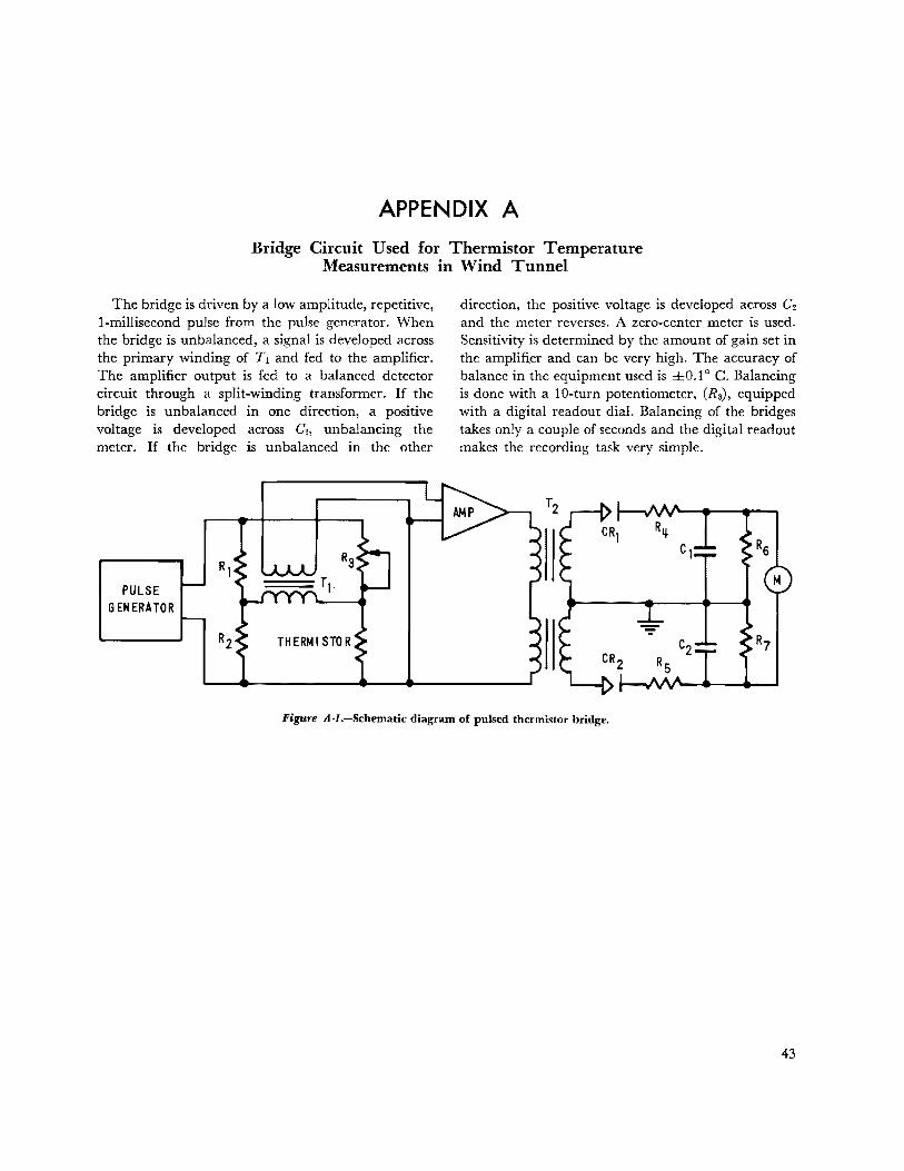
APPENDIX A

Bridge Circuit Used for Thermistor Temperature Measurements in Wind Tunnel

The bridge is driven by a low amplitude, repetitive, 1-millisecond pulse from the pulse generator. When the bridge is unbalanced, a signal is developed across the primary winding of T1 and fed to the amplifier. The amplifier output is fed to a balanced detector circuit through a split-winding transformer. If the bridge is unbalanced in one direction, a positive voltage is developed across ell unbalancing the meter. If the bridge is unbalanced in the other

Rl

PULSE GENERATOR

R2 THERMISTOR

direction, the positive voltage is developed across c2 and the meter reverses. A zero-center meter is used. Sensitivity is determined by the amount of gain set in the amplifier and can be very high. The accuracy of balance in the equipment used is ±0.1 ° C. Balancing is done with a 10-turn potentiometer, (R3), equipped with a digital readout dial. Balancing of the bridges takes only a couple of seconds and the digital readout makes the recording task very simple.

Rs

M

R7

Figure .4·1.-Schematic diagram of puJsed. thermistor bridge.

43

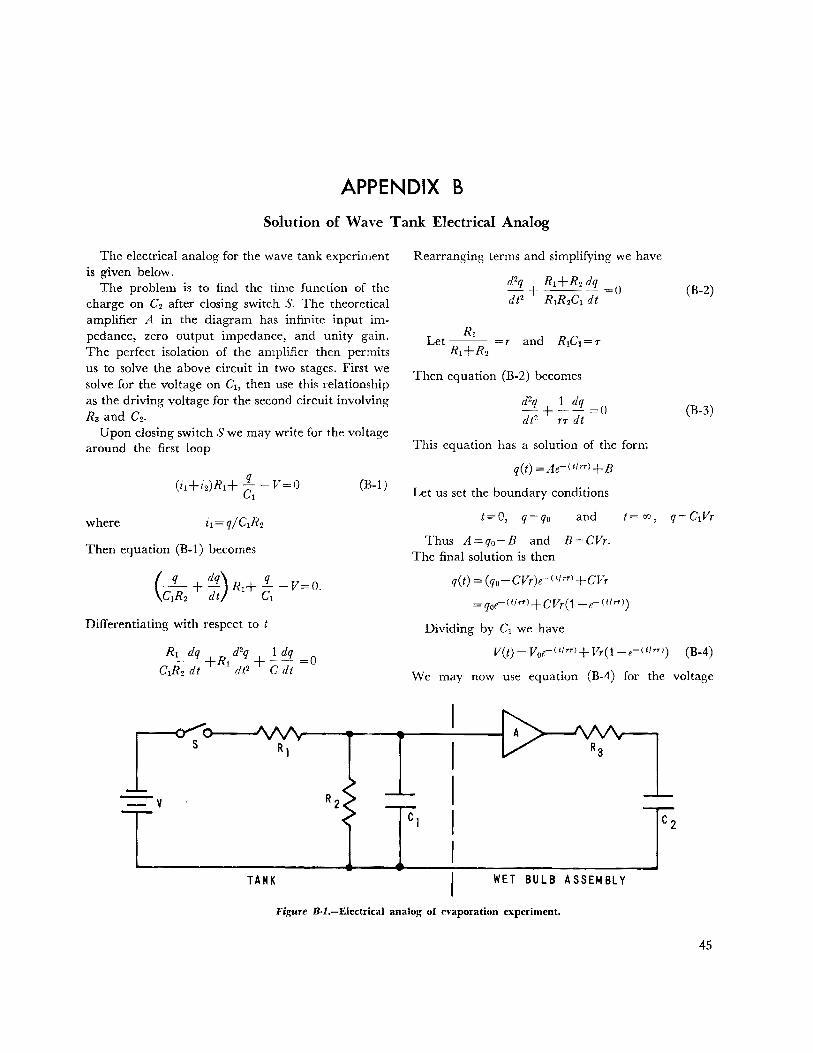
APPENDIX B Solution of Wave Tank Electrical Analog

The electrical analog for the wave tank experiment is given below.

The problem is to find the time function of the charge on C2 after closing switch S. The theoretical amplifier A in the diagram has infinite input im­pedance, zero output impedance, and unity gain. The perfect isolation of the amplifier then permits us to solve the above circuit in two stages. First we solve for the voltage on C1, then use this relationship as the driving voltage for the second circuit involving R3 and C2.

Upon closing switch S we may write for the voltage around the first loop

(B-1)

where

Then equation (B-1) becomes

Differentiating with respect to t

Rearranging terms and simplifying we have

Rt Let--- = r and R1C1 = r

R1+R2

Then equation (B-2) becomes

rPq 1 dq -+--=0 dt2 rr dt

This equation has a solution of the form

q(t) =Ae-<tfrr>+B

Let us set the boundary conditions

t=O, q=qo and

Thus A=qo-B and B=CVr. The final solution is then

q(t) = (qo-CVr)e-<tlrr>+CVr

=qoe-(t/rr>+CVr(1-e-<tlrr>)

Dividing by C1 we have

(B-2)

(B-3)

V(t) = V0e-<tf,..,.>+ Vr(1-r<ttrrl) (B-4)

We may now use equation (B-4) for the voltage

TANK WET BULB ASSEMBLY

Figure B·l.-Electrical analog of evaporation experiment.

45

applied to RaC2• Equating the voltages around the second loop we have

qo q,. where Vo=- and Vr= C ·

c2 2

Dividing by R3 we have

dq q qo q,. _ + _ = _ e-<tl,...>+ _ (1-e-<t!rrl) (B-5) dt Tm Tm Tm

Equation (B-5) may be integrated by using the inte­grating factor e< 1f .. ,.>. Multiplying both sides of equation (B-5) by e<*ml we have

q(t)= rr(qo-q,.) e!t(,..,._.,.m)/1'1Tmle-<tfr,.) rr-r,.

+q,.+ Ke-<tlrm)

q(t)=q,.+ rr(qo-qm) e-W,...>+Ke-<tfr.,) rr-r,.

(B-6)

Apply boundary condition q(t) = qo when t = 0

K . rr(qo-q,.) =qo-q,.- (B-7)

rr-r,.

Combining equations (B-6) and (B-7) and ar-

46

ranging terms we have

(t) + (qo-q,.)rr -<tlrr>+ (q,.-qo)r,. ..-(t/r > q =~ e • m

rr-r,. rr-r,.

(B-8)

Equation (B-8) is the solution of the electrical circuit where q is the charge on the Capacitors C2.

Going to the tank experiment, q becomes the specific humidity and the boundary conditions are

qo = equilibrium specific humidity at start of experiment

q, = saturation specific humidity at the water temperature

q,. = maximum specific humidity reached at t~ oo r=qm/q •.

The other terms in equation (B-8) become

r = actual time constant of experiment if no air leakage were present

r,.= time constant of wet bulb.

Equation (B-8) thus becomes the solution to the evaporation experiment. Adding (q,.-q0) to both sides of equation (B-8) and rearranging terms we have

q(t) = qo+ (q,.- qo)

Taking q0 to the left side of the equation and dividing through by (q,.-q0) we have

and therefore

[ 1- q-qo] = __:.::_e-(1/rr)_ ~6-(t/r.,.) q .. -qo rr-r,. rr-r,.

(B-9)

Equation (B-9) is in a normalized form where only time constants are important. The start time and end points do not displace the experimental curve if the time constants remain fixed. This form permits much better comparison of the experimental results.

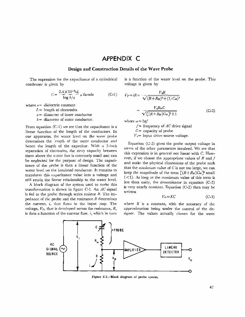
APPENDIX C Design-and Construction Details of the Wave Probe

The expression for the capacitance of a cylindrical condenser is given by

C 2.4X10-7EL r d = p.1ara s

log b/a

where E = dielectric constant L = length of electrodes a= diameter of inner conductor b = diameter of outer conductor.

(C-1)

From equation (C-1) we see that the capacitance is a linear function of the length of the conductors. In our apparatus, the water level on the wave probe determines the length of the outer conductor and hence the length of the capacitor. With a 3-inch separation of electrodes, the stray capacity between them above the water line is extremely small and can be neglected for the purpose of design. The capaci­tance of the probe is then a linear function of the water level on the insulated conductor. It remains to transform this capacitance value into a voltage and still retain the linear relationship to the water level.

A block diagram of the system used to make this transformation is shown in figure C-1. An AC signal is fed to the probe through series resistor R. The im­pedance of the probe and the resistance R determines the current, i, that flows in the input loop. The voltage, Vp, that is developed across the resistance, R, is then a function of the current flow, i, which in turn

AC Sl GNAL rv SOURCE

is a function of the water level on the probe. This voltage is given by

VoRwC = -Vr::[=(R=+~R=w=)C=w===]2=+=1

where w=21f'j f = frequency of AC drive signal C= capacity of probe v.= input drive source voltage.

(C-2)

Equation (C-2) gives the probe output voltage in terms of the other parameters involved. We see that this expression is in general not linear with C. How­ever, if we choose the appropriate values of R andj and make the physical dimensions of the probe such that the maximum value of C is not too large, we can keep the magnitude of the term [(R+Rw)Cw]2 small ( < 1). As long as the maximum value of this term is less than unity, the denominator in equation (C-2) is very nearly constant. Equation (C-2) then may be written

(C-3)

where K is a constant, with the accuracy of the approximation being under the control of the de­signer. The values actually chosen for the wave

LINEAR DETECTOR

Figure C·I.-Block diagram of probe system.

47

~

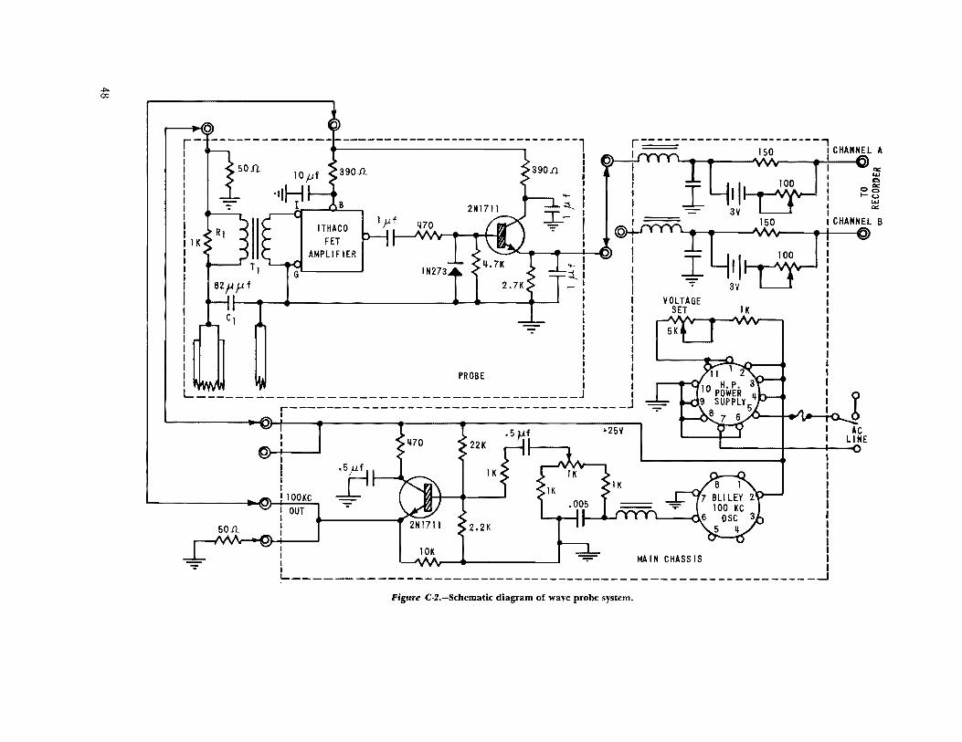
r- -----------------------------,

lK

I

PROBE : ' .. , W •• r• I L--------------------------------------J

50.11.

~--------------------------------------J I

I I I

.S(fl

IOK

22K

lK

2.2K

..... MAIN CHASSIS

L--------------------------------------------------------...J Figure C·2.-5c:hematic diagram of wave probe system.

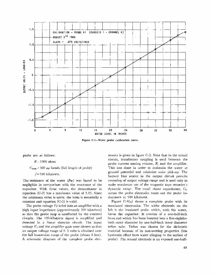
"" "' I 0

a _,

1.5

1.0

0.5

-1.0

x---~ -1.5

CALIBRATION - PROBE 'I (CHASSIS AUGUST srd 1966

SLOPE = .075 VOLTS/INCH

/ ,.,..,

/ v

v v /

I - CHANNEL A) ,., .... .:J ...,.

/ v

/ /

v /

v

/ /

v

0 8 12 16 20 2ij WATER LEVEL IN INCHES

28 32 36 '10

Figure C-J.-Wave probe calibration curve.

probe are as follows:

R=1000 ohms

Cmax = 500 p.p. farads {full length of probe)

j = 100 kilohertz.

The resistance of the water (Rw) was found to be negligible in comparison with the reactance of the capacitor. With these values, the denominator in equation (C-2) has a maximum value of 1.05. Since the minimum value is unity, the term is essentially a constant and equation (C-3) is valid.

The probe voltage Vp is fed into an amplifier with a high input impedance (approximately 300 kiloohms) so that the probe loop is unaffected by the external circuits. The tOO-kilohertz signal is amplified and detected in a linear detector circuit. The input voltage v. and the amplifier gain were chosen so that an output voltage range of Q-3 volts is obtained over the full immersion range of the probe (about 4 feet). A schematic diagram of the complete probe elec-

tronics is given in figure C-2. Note that in the actual circuit, transformer coupling is used between the probe current sensing resistor, R, and the amplifier. This was done in order to maintain the water at ground potential and minimize noise pick-up. The battery bias source in the output circuit permits centering of output voltage range and is used only to make maximum use of the magnetic tape recorder's dynamic range. The small shunt capacitance, C~>

across the probe electrodes tunes out the probe in­ductance at 100 kilohertz.

Figure C-4{a) shows a complete probe with its associated electronics. The white electrode on the left is the insulated probe which, with the water, forms the capacitor. It .consists of a one-half-inch brass rod which has been inserted into a five-eighths­inch outer diameter by one-half-inch inner diameter teflon tube. Teflon was chosen for the dielectric material because of its non-wetting properties (less hysteresis effect from water clinging to the surface of probe). The second electrode is an exposed one-half-

49

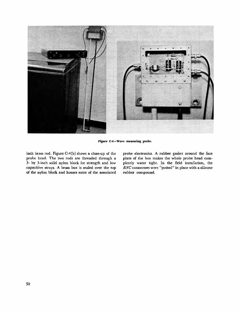
Figure C-4.-Wave measuring probe.

inch brass rod. Figure C-4(b) shows a close-up of the probe head. The two rods are threaded through a 3- by 3-inch solid nylon block for strength and low capacitive strays. A brass box is sealed over the top of the nylon block and houses some of the associated

so

probe electronics. A rubber gasket around the face plate of the box makes the whole probe head com­pletely water tight. In the field installation, the BNC connectors were "potted" in place with a silicone rubber compound.

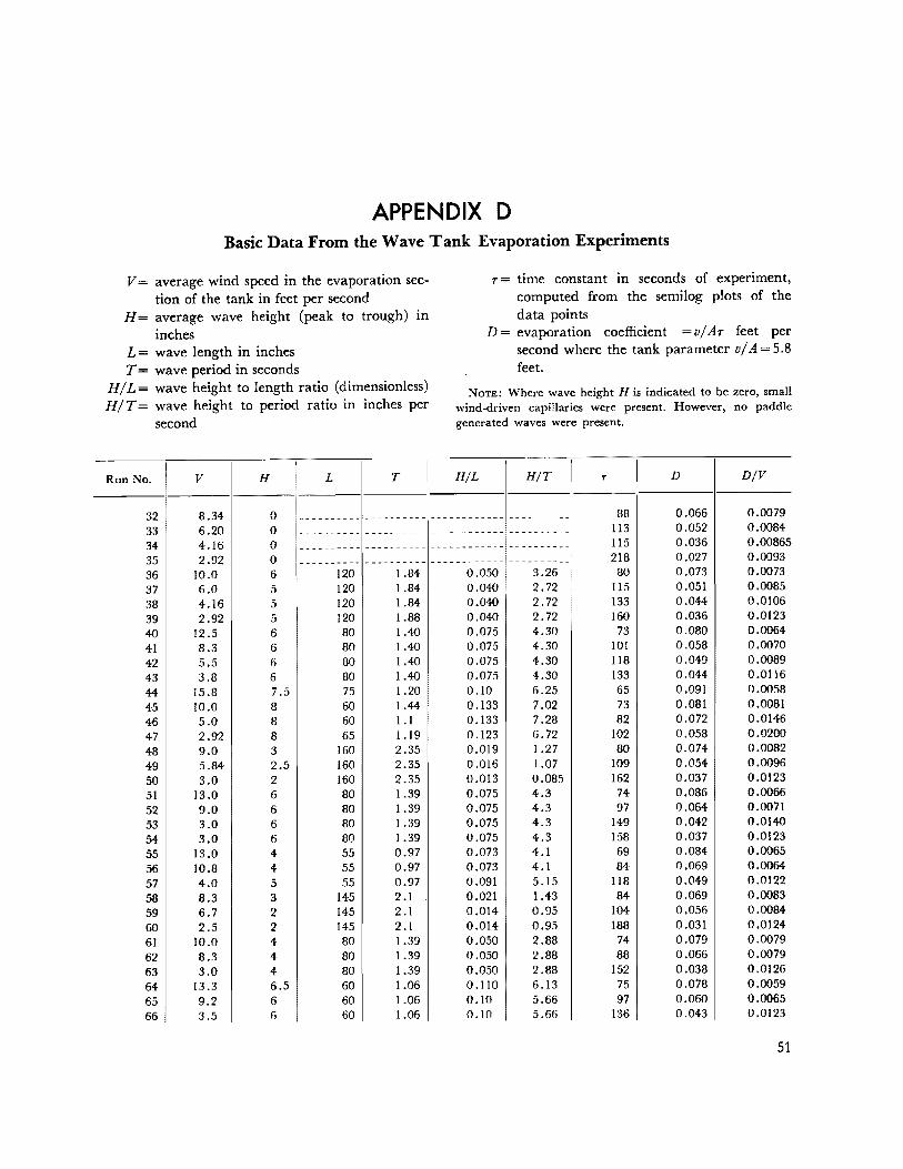
APPENDIX D Basic Data From the Wave Tank Evaporation Experiments

V = average wind speed in the evaporation sec­tion of the tank in feet per second

H = average wave height (peak to trough) in inches

L = wave length in inches T = wave period in seconds

H/L= wave height to length ratio (dimensionless) H/T= wave height to period ratio in inches per

second

Run No. v I H L T

32 8.34 0 ---------- ----------33 6.20 0

__ ... _______ ----------

34 4.16 0 ---------- ----------35 2.92 0 ---------- ----------36 10.0 6 120 1.84 37 6.0 5 120 1.84 38 4.16 5 120 1.84 39 2.92 5 120 1.88 40 12.5 6 80 1.40 41 8.3 6 80 1.40 42 5.5 6 80 1.40 43 3.8 6 80 1.40 44 15.8 7.5 75 1.20 45 10.0 8 60 1.44 46 5.0 8 60 1.1 47 2.92 8 65 1.19 48 9.0 3 160 2.35 49 5.84 2.5 160 2.35 50 3.0 2 160 2.35 51 13.0 6 80 1.39 52 9.0 6 80 1.39 53 3.0 6 80 1.39 54 3.0 6 80 1.39 55 13.0 4 55 0.97 56 10.8 4 55 0.97 57 4.0 5 55 0.97 58 8.3 3 145 2.1 59 6.7 2 145 2.1 60 2.5 2 145 2 .l 61 10.0 4 80 1.39 62 8.3 4 80 1.39 63 3.0 4 80 1.39 64 13.3 6.5 60 1.06 65 9.2 6 60 1.06 66 3.5 6 60 1.06

T= time constant in seconds of experiment, computed from the semilog plots of the data points

D = evaporation coefficient = vj AT feet per second where the tank parameter v/ A= 5.8 feet.

NoTE: Where wave height His indicated to be zero, small wind-driven capillaries were present. However, no paddle generated waves were present.

H/L H/T .,. D D/V

------------ ---------- 88 0.066 0.0079

------------ ---------- 113 0.052 0.0084

------------ ---------- 115 0.036 0.00865

------------ ---------- 218 0.027 0.0093 0.050 3.26 80 0.073 0.0073 0.040 2.72 115 0.051 0.0085 0.040 2.72 133 0.044 0.0106 0.040 2.72 160 0.036 0.0123 0.075 4.30 73 0.080 0.0064 0.075 4.30 101 0.058 0.0070 0.075 4.30 liB 0.049 0.0089 0.075 4.30 133 0,044 0.0116 0.10 6.25 65 0.091 0.0058 0.133 7.02 73 0.081 0.0081 0.133 7.28 82 0.072 0.0146 0.123 6.72 102 0.058 0.0200 0.019 1.27 80 0.074 0.0082 0.016 1.07 109 0.054 0.0096 0.013 0.085 162 0.037 0.0123 0.075 4.3 74 0.086 0.0066 0.075 4.3 97 0.064 0.0071 0.075 4.3 149 0.042 0.0140 0.075 4.3 158 0.037 0.0123 0.073 4.1 69 0.084 0.0065 0.073 4.1 84 0.069 0.0064 0.091 5.15 118 0.049 0.0122 0.021 1.43 84 0.069 0.0083 0.014 0.95 104 0.056 0.0084 0.014 0.95 188 0.031 0.0124 0.050 2.88 74 0.079 0.0079 0.050 2.88 88 0.066 0.0079 0.050 2.88 152 0.038 0.0126 0.110 6.13 75 0.078 0.0059 0.10 5.66 97 0.060 0.0065 0.10 5.66 136 0.043 0.0123

51

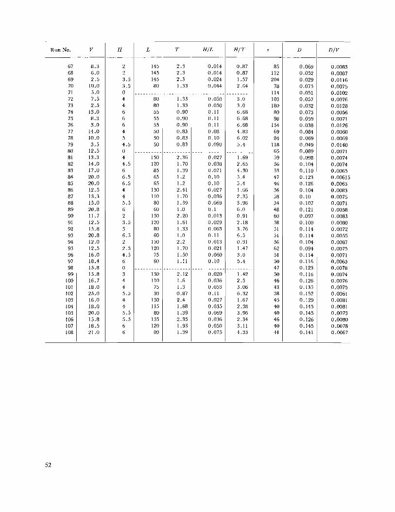
Run No. v H L T H/L H/T T D D/V

67 8.3 2 145 2.3 0.014 0.87 85 0.069 0.0083 68 6.0 2 145 2.3 0.014 0.87 112 0.052 0.0087 69 2.5 3.5 145 2.3 0.024 1.57 204 0.029 0.0116 70 10.0 3.5 80 1.33 0.044 2.64 78 0.075 0.0075 71 5.0 0 ---------- ---------- ------------ ---------- 114 0.051 0.0102 72 7.5 4 80 1.33 0.050 3.0 103 0.057 0.0076 73 2.5 4 80 1.33 0.050 3.0 180 0.032 0.0128 74 13.0 6 55 0.90 0.11 6.68 80 0.073 0.0056 75 8.3 6 55 0.90 0.11 6.68 98 0.059 0.0071 76 3.0 6 55 0.90 0.11 6.68 154 0.038 0.0126 77 14.0 4 50 0.83 0.08 4.83 69 0.084 0.0060 78 10.0 5 50 0.83 0.10 6.02 84 0.069 0.0069 79 3.5 4.5 50 0.83 0.090 5.4 118 0.049 0.0140 80 12.5 0 ---------- ---------- ------------ ---------- 65 0.089 0.0071 81 13.3 4 150 2.36 0.027 1.69 59 0.098 0.0074 82 14.0 4.5 120 1.70 0.038 2.65 56 0.104 0.0074 83 17.0 6 85 1.39 0.071 4.30 53 0.110 0.0065 84 20.0 6.5 65 1.2 0.10 5.4 47 0.123 0.00615 85 20.0 6.5 65 1.2 0.10 5.4 46 0.126 0.0063 86 12.5 4 150 2.41 0.027 1.66 56 0.104 0.0083 87 13.3 4 110 l. 70 0.036 2.35 58 0.10 0.0075 88 15.0 5.5 80 1.39 0.069 3.96 54 0.107 0.0071 89 20.8 6 60 1.0 0.1 6.0 48 0.121 0.0058 90 11.7 2 150 2.20 0.013 0.91 60 0.097 0.0083 91 12.5 3.5 120 1.61 0.029 2.18 58 0.100 0.0080 92 15.8 5 80 1.33 0.063 3.76 51 0.114 0.0072 93 20.8 6.5 60 1.0 0.11 6.5 51 0.114 0.0055 94 12.0 2 150 2.2 0.013 0.91 56 0.104 0.0087 95 12.5 2.5 120 1.70 0.021 1.47 62 0.094 0.0075 96 16.0 4.5 75 1.50 0.060 3.0 51 0.114 0.0071 97 18.4 6 60 1.11 0.10 5.4 50 0.116 0.0063 98 15.8 0 ---------- ---------- ------------ ---------- 47 0.123 0.0078 99 15.8 3 150 2.12 0.020 1.42 50 0.116 0.0074

100 16.7 4 110 1.6 0.036 2.5 46 0.126 0.0076 101 18.0 4 75 1.3 0.053 3.06 43 0.135 0.0075 102 25.0 5.5 50 0.87 0.11 6.32 38 0.152 0.0061 103 16.0 4 150 2.4 0.027 1.67 45 0.129 0.0081 104 18.0 4 115 1.68 0.035 2.38 40 0.145 0.0081 105 20.0 5.5 80 1.39 0.069 3.96 40 0.145 0.0073 106 15.8 5.5 155 2.35 0.036 2.34 46 0.126 0.0080 107 18.5 6 120 1.93 0.050 3.11 40 0.145 0.0078 108 21.0 6 80 1.39 0.075 4.33 41 0.141 0.0067

I

52

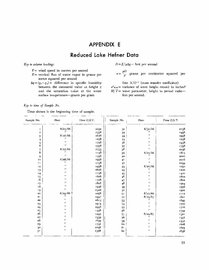
APPENDIX E

~educed Lake Hefner Data

Key to column headings

V =:= wind speed in meters per second E = vertical flux of water vapor in grams per

meter squared per second llq = (q.-q.) = difference in specific humidity

between the measured value at height ~ and the saturation value at the water surface temperature--grams per gram

Key to time of Sample No.

Time shown is the beginning time of sample.

Sample No. Date Time C.S.T.

I 8/2s/66 2032 2 ,

2358 3 8/26/66 o6ll8 ·4

II 1258 5

, 1758

6 II 2358 7 8/ll?/66 0753 8 ,

II 58 9

II 1558 IO 8/ll8/66 1958 II

II 0158 Ill

, 0458

13 II o8l!8 14 II 1158 15 II 16ll8 16 II I7ll8 17 II 1828 18 II 1958 19 II 2328 liO 8/29/66 0058 21 II 0447 22 II o613 23 II 0913 24 II 0948 25

, 1348

26 II 1443 27

, 1559

28 If 1649 29 II 1752 go

, li058

31 " ll3liB

D=E/pll.q- feet per second

pD . n = V grams per centimeter squared per

foot X 10-5 (mass transfer coefficient) u2wH = variance of wave height record in inches2

H/T= wave parameter, height to period ratio­feet per second.

Sample No. Date Time C.S.T.

32 8f3o/66 0158 33

, 0458

34 II 0958 35 II 1258 36 II 1458 37 II 1758 38 " 2238 39 8/ll5/66 1815 40

, liOOO 41 II liOI6 42 II ll034 43 8/ll6/66 1050 44 II

IliOO

45 ,

1400 46 " 1800 47 If I8llll 48 " 1924 49 " 1956 so II 1902 51 8/27/66 IIIli 52 8/25/67 1621 53 II 1645 54 II 1700 55 If 1716 s6

, 1732

57 8/llg/67 15lll 58 II

1537 59

, 155ll

6o , 16o8

61 , 1623

62 " 1636

53

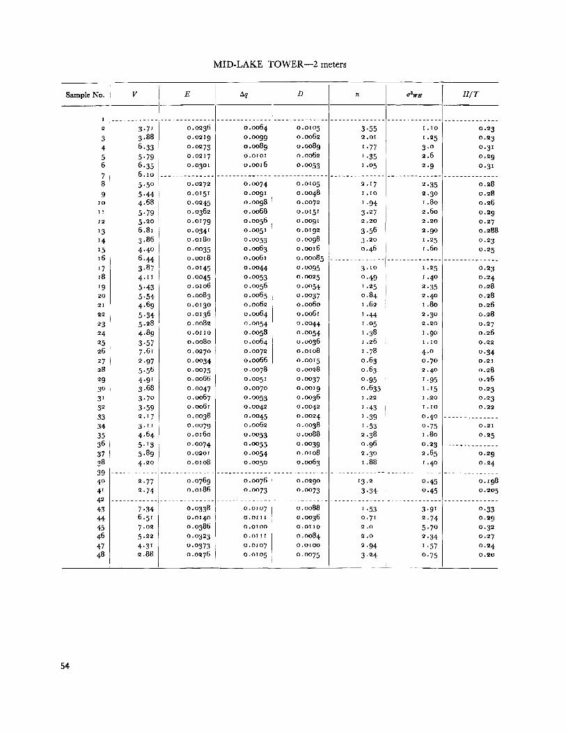
MID-LAKE TOWER-2 meters

Sample No. v E tlq D n ulwa H/T

I ------------ --~------------ --------------_________ ... ____

-------------- -------------- --------------II 3·71 0.01136 0.0o64 0.0105 3·55 1.10 0.23 3 3·88 0.01119 o.o099 o.oo62 11.01 1.25 0.23 4 6.33 0.01173 o.oo89 o.oo89 1·77 3·0 0.31 5 5·79 0.01117 0.0101 o.oo62 1·35 2.6 Oo!l9 6 6.35 0.0301 0.0016 0.0053 1.05 !l.9 0,31 7 6.10 --------------

___ .,. __________ -------------- -------------- -------------- --------------

8 5·5° 0.0272 0.0074 0.0105 2.17 2·35 0.28 9 5·44 0.0151 o.oogr o.oo-4-8 I ,10 2.30 0.28

10 4.68 0.0245 o.oog8 0.0072 !.94 !.So 0.26 I! 5·79 0.0362 o.oo68 0.0151 3·27 2.6o o.29 12 5·20 0.0179 o.oo56 o.oo91 2.20 12.20 0.27 13 6.81 0.0341 0.0051 0.0192 3·56 2.90 0.288 14 3.86 o.o18o 0.0053 o.oo98 3·20 1.25 0.23 15 4·40 0.0035 o.oo63 0.00!6 0.46 1.6o 0.25 16 6.44 o.oo18 o.oo61 o.ooo85 -------------- -------------- --------------17 3·87 0.0145 0.0044 0.0095 3·10 1.25 0.23 18 4·11 0.0045 0.0053 0.0025 0·49 1.40 0.24 19 5·43 o.o106 o.oo56 0.0054 1.25 2·35 0.28 20 5·54 o.oo83 o.oo6s 0.0037 o.84 2.40 0.28 21 4•69 0.0130 o.oo62 o.oo6o 1.62 t,8o 0.26 22 5·34 0.0136 0.0064 0.0061 1.44 2.30 0.28 23 5·28 o.oo82 0,0054 0.0044 !.05 2.20 0.27 24 4·89 0,0110 o.oos8 0.0054 1.38 1.90 0.26 25 3·57 o.oo8o 0.0004 0.0036 !.26 1.10 0.22 26 7·61 0.0270 0.0072 0.0!08 1.78 4·0 0·34 27 2·97 0.0034 o.oo66 0.0015 0.63 0.70 0.21 28 5·56 0.0075 0.0078 0.0028 o.63 2.40 0.28 29 4·91 o.oo66 0.0051 0.0037 o.gs 1.95 0.26 30 3.68 0.0047 0.0070 0.0019 o.635 I .15 0.23 31 3·70 o.oo67 0.0053 0.0036 1.22 1.20 0.23 32 3·59 o.oo61 0.0042 0.0042 1.43 I .10 0.22 33 2.17 0.0038 0.0045 0.0024 1.39 0.40 --------------34 3.11 0.0079 o.oo62 o.oo38 I •53 0·75 0.111 35 4·64 0.016o 0.0053 o.oo88 2.38 1.80 0.115 36 5·13 0.0074 0.0055 0.0039 o.g6 0.23 --------------37 5·89 0.0201 0.0054 o.o1o8 2.30 2.65 0.29 38 4·20 o.o1o8 0.0050 o.oo63 !.88 1.40 0.24 39 ------------ -------------- -------------- -------------- -------------- -------------- --------------40 2·77 o.o769 o.oo76 0.0290 13.11 0·45 0.198 41 2·74 o.or86 0.0073 0.0073 3·34 Oo45 0.205 42 ------------ -------------- ------------ ..... -------------- -------------- --------------

______ .,... _______

43 7·34 0.0338 0.0107 o.oo88 I •53 3·91 0·33 44 6.51 0.0140 O.OIIJ o.oo36 0.7J 2·74 0.29 45 7·02 0.0386 0.0100 0.0110 2.0 5·70 0.32 46 5·22 0.0323 0.0111 o.oo84 2.0 2·34 0.27 4:7 4·31 0.0373 0.0107 0.0100 2·94 I •57 0.24 48 2.88 0.0276 0.0105 0.0075 3·24 0·75 0.20

54

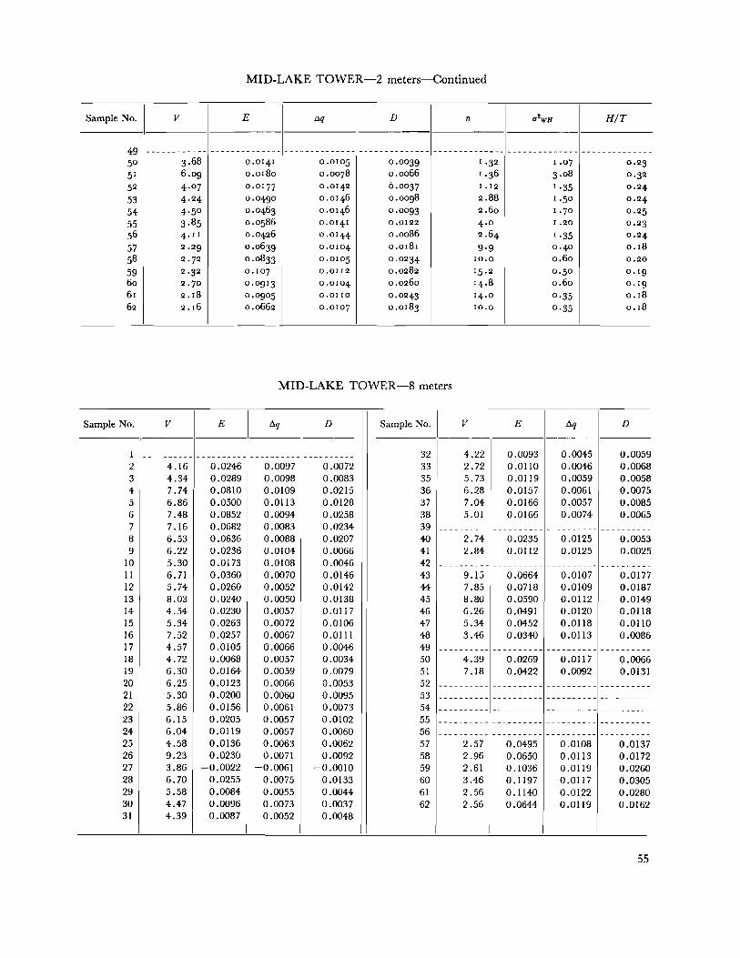
MID-LAKE TOWER-2 meters-Continued

Sample No. v E Aq D n vlJvH H/T

49 ------------ -------------- -------------- -------------- -------------- -------------- --------------so 3.68 0.0141 0.0105 0.0039 1.32 1.07 0.23 51 6.og 0.0180 0.0078 o.oo66 1.36 3·o8 0.32 52 4·07 0.0177 0.0142 0.0037 1.12 1.35 0.24 53 4·24 Oo0490 0.0146 o.oog8 2.88 !.50 0.24 54 4·50 0.0463 0.0146 0.0093 2.6o !.70 0.25 55 3·85 o.os86 0.0141 0.0122 4·0 1.20 0.23 s6 4·11 0.0426 0.0144 o.oo86 2.64 1.35 0.24 57 2.2g 0.0039 0.0104 0.0181 9·9 0.40 0.18 sa 2.72 o.o833 0.0105 0.0234 10.0 o.6o 0.20 59 2.32 0.107 0.0112 0,0282 15.2 o.so 0.19 6o 2.70 o.og13 0.0104 o.o26o 14.8 o.6o 0,19 6r 2.!8 o.ogos 0.0110 0.0243 14.0 0·35 0.18 62 2.16 o.o662 0.0107 0.0183 10.0 0·35 0.18

MID-LAKE TOWER-S meters

Sample No. v E ~ D Sample No. v E ~ D

I ---------- ---------- ---------- ---------- 32 4.22 0.0093 0.0045 0.0059 2 4.16 0.0246 0.0097 0.0072 33 2.72 0.0110 0.0046 0.0068 3 4.34 0.0289 0.0098 0.0083 35 5.73 0.0119 0.0059 0.0058 4 7.74 0.0810 0.0109 0.0215 36 6.28 0.0157 0.0061 0.0075 5 6.86 0.0500 0.0113 0.0128 37 7.04 0.0166 0.0057 0.0085 6 7.48 0.0852 0.0094 0.0258 38 5.01 0.0166 0.0074 0.0065 7 7.16 0.0682 0.0083 0.0234 39 ---------- ---------- ---------- ----------8 6.53 0.0636 0.0088 0.0207 40 2.74 0.0235 0.0125 0.0053 9 6.22 0.0236 0.0104 0.0066 41 2.84 0.0112 0.0125 0.0025

10 5.30 0.0173 0.0108 0.0046 42 ---------- ---------- ---------- ----------II 6.71 0.0360 0.0070 0.0146 43 9.15 0.0664 0.0107 0.0177 12 5.74 0.0260 0.0052 0.0142 44 7.85 0.0718 0.0109 0.0187 13 8.03 0.0240 0.0050 0.0138 45 8.80 0.0590 0.0112 0.0149 14 4.54 0.0230 0.0057 0.0117 46 6.26 0.0491 0.0120 0.0118 15 5.34 0.0263 0.0072 0.0106 47 5.34 0.0452 0.0118 0.0110 16 7.52 0.0257 0.0067 0.0111 48 3.46 0.0340 0.0113 0.0086 17 4.57 0.0105 0.0066 0.0046 49 ---------- ---------- ---------- ----------18 4.72 0.0068 0.0057 0.0034 50 4.39 0.0269 0.0117 0.0066 19 6.30 0.0164 0.0059 0.0079 51 7 •. 18 0.0422 0.0092 0.0131 20 6.25 0.0123 0.0066 0.0053 52 ---------- ---------- ---------- ----------21 5.30 0.0200 0.0060 0.0095 53 ---------- ---------- ---------- ----------22 5.86 0.0156 0.0061 0.0073 54 ---------- ---------- ---------- ----------23 6.15 0.0205 0.0057 0.0102 55 ---------- ---------- ---------- ----------24 6.04 0.0119 0.0057 0.0060 56 ---------- ---------- ---------- ----------25 4.58 0.0136 0.0063 0.0062 57 2.57 0.0495 0.0108 0.0137 26 9.23 0.0230 0.0071 0.0092 58 2.96 0.0650 0.0113 0.0172 27 3.86 -0.0022 -0.0061 -0.0010 59 2.61 0.1036 0.0119 0.0260 28 6.70 0.0255 0.0075 0.0133 60 3.46 0.1197 0.0117 0.0305 29 5.58 0.0084 0.0055 0.0044 61 2.56 0.1140 0.0122 0.0280 30 4.47 0.0096 0.0073 0.0037 62 2.56 0.0644 0.0119 0.0162 31 4.39 0.0087 0.0052 0.0048

55

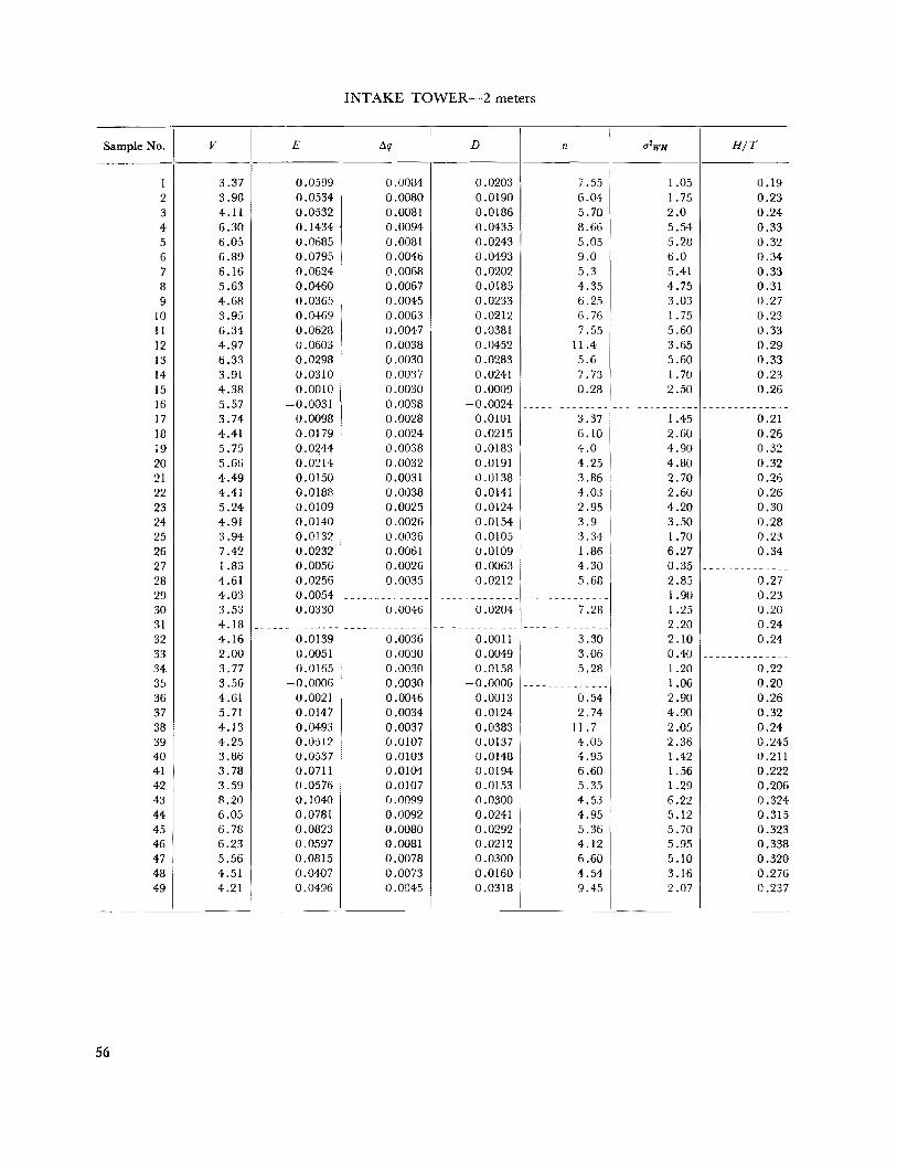
INTAKE TOWER-2 meters

Samp1eNo. v E ilq I

D n tllwn H/T

1 3.37 0.0599 0.0084 0.0203 7.55 1.05 0.19 2 3.98 0.0534 0.0080 0.0190 6.04: 1. 75 0.23 3 4.11 0.0532 0.0081 0.0186 5.70 2.0 0.24 4 6.30 0.1434 0.0094 0.0435 8.66 5.54: 0.33 5 6.05 0.0685 0.0081 0.0243 5.05 5.28 0.32 6 6.89 0.0795 0.0046 0.0493 9.0 6.0 0.34 7 6.16 0.0624 0.0068 0.0202 5.3 5.41 0.33 8 5.63 0.0460 0.0067 0.0185 4.35 4.75 0.31 9 4.68 0.0365 0.0045 0.0233 6.25 3.03 0.27

10 3.95 0.0469 0.0063 0.0212 6.76 1.75 0.23 11 6.34 0.0628 0.0047 0.0381 7.55 5.60 0.33 12 4.97 0.0603 0.0038 0.0452 11.4 3.65 0.29 13 6.33 0.0298 0.0030 0.0283 5.6 5.60 0.33 14 3.91 0.0310 0.0037 0.0241 7.73 1. 70 0.23 15 4.38 0.0010 0.0030 0.0009 0.28 2.50 0.26 16 5.57 -0.0031 0.0038 -0.0024 -------------- -------------- --------------17 3.74 0.0098 0.0028 0.0101 3.37 1.45 0.21 18 4.41 0.0179 0.0024 0.0215 6.10 2.60 0.26 19 5.75 0.024:4: 0.0038 0.0183 4.0 4.90 0.32 20 5.66 0.0214 0.0032 0.0191 4.25 4.80 0.32 21 4.49 0.0150 0.0031 0.0138 3.86 2.70 0.26 22 4.41 0.0188 0.0038 0.0141 4.03 2.60 0.26 23 5.24 0.0109 0.0025 0.0124 2.95 4.20 0.30 24 4.91 0.0140 0:0026 0.0154 3.9 3.50 0.28 25 3.94 0.0132 0.0036 0.0105 3.34 1.70 0.23 26 7.42 0.0232 0.0061 0.0109 1.86 6.27 0.34 27 1.83 0.0056 0.0026 0.0063 4.30 0.35 --------------28 4.61 0.0256 0.0035 0.0212 5.68 2.85 0.27 29 4.03 0.00,54 -------------- -------------- -------------- 1.90 0.23 30 3.53 0.0330 0.0046 0.0204 7.28 1.25 0.20 31 4.18 __________ , ..... _

--------------_ ________ .. _ .... __

-------------- 2.20 0.24 32 4.16 0.0139 0.0036 0.0011 3.30 2.10 0.24 33 2.00 0.0051 0.0030 0.0049 3.06 0.40 --------------34. 3.77 0.0165 0.0030 0.0158 5.28 1.20 0.22 35 3.56 -0.0006 0.0030 -0.0006 -------------- 1.06 0.20 36 4.61 0.0021 0.0046 0.0013 0.54 2.90 0.26 37 5.71 0.0147 0.0034 0.0124 2.74 4.90 0.32 38 4.13 0.0493 0.0037 0.0383 11.7 2.05 0.24 39 4.25 0.0512 0.0107 0.0137 4.05 2.36 0.245 40 3.86 0.0537 0.0103 0.0148 4.95 1.42 0.211 41 3.78 0.0711 0.0104 0.0194 6.60 1.56 0.222 42 3.59 0.0576 0.0107 0.0153 5.35 1.29 0.206 43 8.20 0.104:0 0.0099 0.0300 4.53 6.22 0.324 44 6.05 0.0781 0.0092 0.0241 4.95 5.12 0.315 45 6.78 0.0823 0.0080 0.0292 5.36 5.70 0.323 46 6.23 0.0597 0.0081 0.0212 4.12 5.95 0.338 47 5.56 0.0815 0.0078 0.0300 6.60 5.10 0.320 48 4.51 0.0407 0.0073 0.0160 4.54 3.16 0.276 49 4.21 0.0496 0.0045 0.0318 9.45 2.07 0.237

56

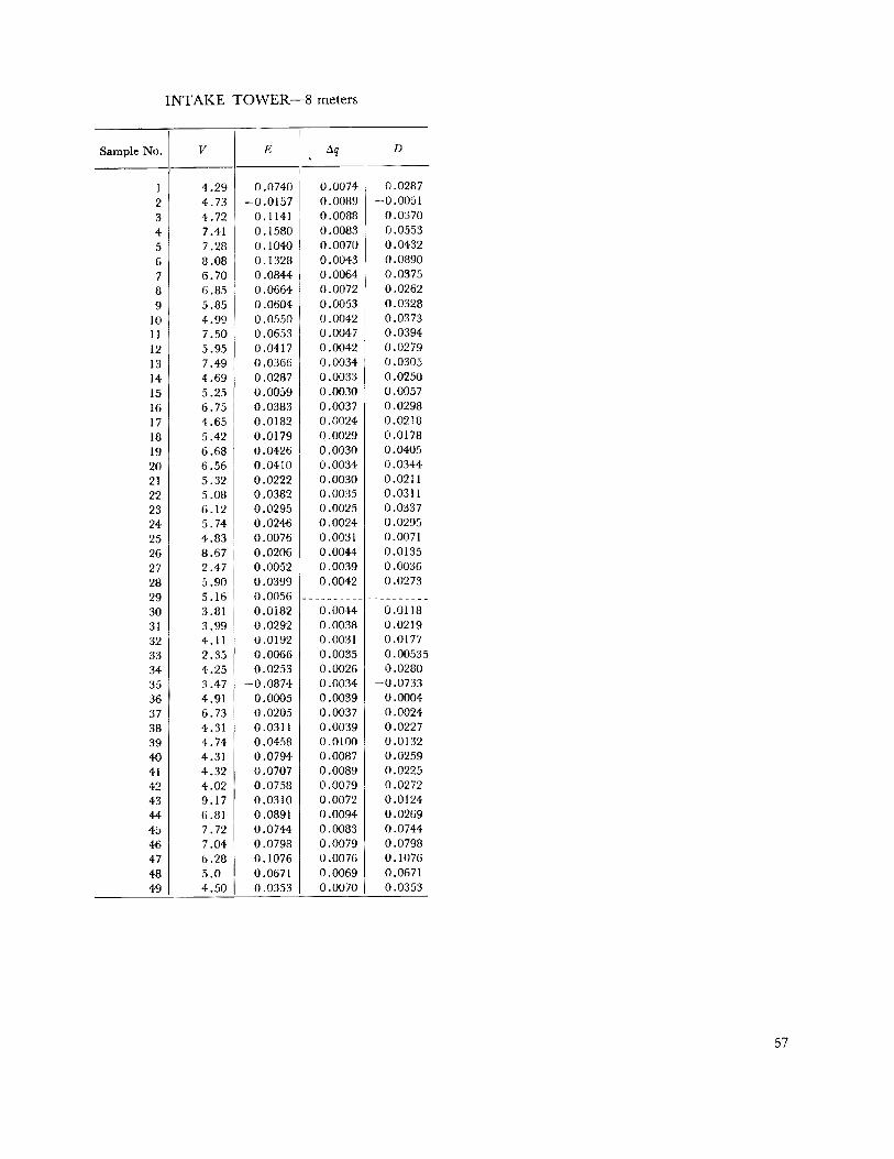
INTAKE TOWER-S meters

Sample No. v E AtJ D . 1 4.29 0.0740 0.0074 0.0287 2 4.73 -0.0157 0.0089 -0.0051 3 4.72 0.1141 0.0088 0.0370 4 7.41 0.1580 0.0083 0.0553 5 7.28 0,1040 0.0070 0.0432 6 8.08 0.1328 0.0043 0.0890 7 6.70 0.0844 0.0064 0.0375 8 6.85 0.0664 0.0072 0.0262 9 5.85 0.0604 0.0053 0.0328

10 4.99 0.0550 0.0042 0.0373 11 7.50 0.0653 0.0047 0.0394 12 5.95 0.0417 0.0042 0.0279 13 7.49 0.0366 0.0034 0.0305 14 4.69 0.0287 0.0033 0.0250 15 5.25 0.0059 0.0030 0.0057 16 6.75 0.0383 0.0037 0.0298 17 4.65 0.0182 0.0024 0.0218 18 5.42 0.0179 Q.0029 0.0178 19 6.68 0.0426 0.0030 0.0405 20 6.56 0.0410 0.0034 0.0344 21 5.32 0.0222 0.0030 0.0211 22 5.08 0.0382 0.0035 0.0311 23 6.12 0.0295 0.0025 0.0337 24 5.74 0.0246 0.0024 0.0295 25 4.83 0.0076 0.0031 0.0071 26 8.67 0.0206 0.0044 0.0135 27 2.47 0.0052 0.0039 0.0036 28 5.90 0.0399 0.0042 0.0273 29 5.16 0.0056 ---------- ----------30 3.81 0.0182 0.0044 0.0118 31 3.99 0.0292 0.0038 0.0219 32 4.11 0.0192 0.0031 0.0177 33 2.35 0.0066 0.0035 0.00535 34 4.25 0.0253 0.0026 0.0280 35 3.47 -0.0874 0.0034 -0.0733 36 4.91 0.0005 0.0039 0.0004 37 6.73 0.0205 0.0037 0.0024 38 4.31 0.0311 0.0039 0.0227 39 4.74 0.0458 0.0100 0.0132 40 4.31 0.0794 0.0087 0.0259 41 4.32 0.0707 0.0089 0.0225 42 4.02 0.0758 0.0079 0.0272 43 9.17 0.0310 0.0072 0.0124 44 6.81 0.0891 0.0094 0.0269 45 7.72 0.0744 0.0083 0.0744 46 7.04 0.0798 0.0079 0.0798 47 6.28 0.1076 0.0076 0.1076 48 5.0 0.0671 0.0069 0.0671 49 4.50 0.0353 0.0070 0.0353

57

ABSTRACT

The evaporation rate from a water surface is shown to be greatly affected by surface waves in laboratory and field tests. Laboratory experiments were made using a large wave tank-wind tunnel apparatus in which both wind speed and wave parameters could be controlled. The apparatus simulates wave condi­tions on large bodies of water with fetches up to a mile or more. Tank experiments indicate certain combinations of wind speed and well-developed waves produce an evaporation rate lower than the rate under similar wind conditions with no waves present. Investigations of air flow over the waves show that, as wave heights increase, regions of dead air are ob­served leeward of wave crests, and vortices appear in the wave troughs. The partially trapped air appar­ently forms an effective barrier to the vertical trans­port of water vapor. Wave and evaporation measure-

58

ments at Lake Hefner, Oklahoma, were very similar to the laboratory measurements. The Lake Hefner data were adjusted to previously measured evapora­tion coefficient relationships derived from water and energy budget measurements. The resulting evapora­tion coefficient curve is believed to give an improved measure of the instantaneous evaporation rate from Lake Hefner under given conditions for wind speed, water surface temperature, and ambient humidity. DESCRIPTORS-*evaporation/evaporation control /waves/ *waves (water)/ wind tunnels/ wind veloc­ity / wind speed / water vapor / water temperature / *reservoir evaporation /lakes / laboratory tests / field investigations. IDENTIFIERS-*evaporation coefficient/ evapora­tion tanks / Lake Hefner, Okla. /wave tanks/ *wave height / mass transport.

* U ••• GOVERNMENT PRINTING OFPIC:E• IIIII ~

Partial List of

Water Resources Technical Publications*

ENGINEERING MONOGRAPHS

No.

31 Ground-Water Movement 32 Stress Analysis of Wye Branches 33 Hydraulic Design of Transitions for Small Canals 34 Control of Cracking in Mass Concrete Structures 35 Effect of Snow Compaction on Runoff from Rain on Snow 36 Guide for Preliminary Design of Arch Dams 37 Hydraulic Model Studies for Morrow Point Dam 38 Potential Economic Benefits from the Use of Radioisotopes in Flow Measure­

ments through High-Head Turbines and Pumps

RESEARCH REPORTS

1 Research-Engineering Methods and Materials 2 Aquatic Weed Control Studies 3 Soils Tests Computer Programs 4 Hydraulic Downpull Forces on Large Gates 5 Park Range Atmospheric Water Resources Program-Phase 1 6 Annual Report of Progress on Engineering Research-1965 7 Effects of Monolayers on Insects, Fish and Wildlife-A Reservoir Evaporation

Reduction Study 8 Synthetic Resin Primer for Coal-Tar Enamel 9 Vibration Studies of Monticello Dam

10 Annual Report of Progress on Engineering Research-1966 11 Pile Supported Structures in Lake Deposits 12 Buried Asphalt Membrane Canal Lining 13 Removal of Saline Water from Aquifers 14 Comparison of Analytical and Structural Behavior Results for Flaming Gorge

Dam 15 Annual Report of Progress on Engineering Research-1967 16 Structural Model Tests of Arch Dams-Glen Canyon and Morrow Point Dams 17 Soil as an Engineering Material 18 A Study of the Effects of Waves on Evaporation from Free Water Surfaces

TECHNICAL RECORDS OF DESIGN AND CONSTRUCTION

Trinity River Division Features of the Central Valley Project Morrow Point Dam and Powerplant Foundation Investigations Merritt Dam Flaming Gorge Dam and Powerplant Willard Dam

* For a pamphlet listing other Bureau of Reclamation publications, address Office of Chief Engineer, Attention 841, Denver Federal Center, Denver, Colo. 80225.