Drift Effects on Plasma Waves

A thesis submitted in partial fulfillment of the

requirement for the award of degree of Doctor of Philosophy in Physics

By

Muhammad Fraz Bashir Reg. No. 015-GCU-PHD-PHY-11

Department of Physics

GC University Lahore

God

Grant me serenity to accept the things,

I can’t change;

The courage to change the things, I can;

And the wisdom to know the difference!

Dedicated to

My Father (Bahsir Hussain), My Mother (Aisha Bano)

& My Beloved Wife

(Fatima Zafar)

Research Completion Certificate

It is certified that the research work contained in this thesis entitled

“Drift Effects on Plasma Waves” has been carried out by Mr.

Muhammad Fraz Bashir, Reg. No. 015-GCU-PHD-PHY-11, under my

supervision at Physics Department, GC University Lahore, during his

postgraduate studies for Doctor of Philosophy in Physics.

Supervisor

Prof. Dr. G. Murtaza National Distinguished Professor

Salam Chair in Physics

GC University, Lahore

Submitted Through

Prof. Dr. Riaz Ahmad

Chairman

Department of Physics

GC University, Lahore

Declaration

I, Mr. Muhammad Fraz Bashir, Reg. No. 015-GCU-PHD-PHY-11,

PhD scholar at the Department of Physics, GC University Lahore,

hereby declare that the matter printed in the thesis entitled “Drift Effects

on Plasma Waves” is my own work and has not been printed, or

published or submitted as research work, thesis or publication in any

form in any University/Research Institution etc. in Pakistan or abroad.

Dated: ___________ ___________________

Signature of Deponent

Acknowledgements

First of all, I say my thanks to almighty Allah for all his blessings

enabling me to complete this thesis. Secondly, I express my deep gratitude to

my supervisor Prof. Dr. G. Murtaza for his continuous support, kind guidance,

useful suggestions and moral support throughout my research period. He is

the person who laid down the foundations of plasma physics in the country

and inspired me to work in this area.

I am also extremely grateful to Prof. Dr. Andrei Smolyakov, University

of Saskatchewan (USASK), Saskatoon, Canada who first introduced me to the

Canadian Commonwealth Exchange Program Scholarship-2011 and then to

the study of Geodesic Acoustic Modes (GAMs) in the field of Tokamak Plasmas

and continuously guided and helped me till the final write-up of my thesis. Due

to his arrangements, I really enjoyed the excess to the different facilities of the

USASK like Library, Email, Super-computer lab, Gym, Swimming pool etc. My

time with him at Saskatoon specially the memorable dinner at his home, and

later through email was really fantastic!

I am also thankful to my other international collaborators for the thesis

work R. J. F. Sgalla, Prof. Dr. A. G. Elfimov, Prof. Dr. A. V. Melnikov and

Prof. Dr. M. Salimullah for their useful discussions and suggestions.

I also appreciate Prof. Dr. Peter H. Yoon who introduces me, at the end

of my PhD, to the exact numerical analysis and the quasi-linear theory using

Fortran which also results in two publications.

I am gratefully obliged to Prof. Dr. Riaz Ahmad, Chairman Physics

Department and also to Prof. Dr. H. A. Shah, ex-Chairman for providing sound

research atmosphere in the department and to Prof. Dr. Tamaz Kaladze for

several fruitful discussions.

I also thank to all my research fellows Gohar Abbas, Muhammad

Jamil, Zafar Iqbal, Hafsa Naim, Sadia Zaheer, Muddasir Ali, Tajammal

Hussain, Fazal Hadi, Naila Noreen and lab fellows Abdur Rasheed, Azhar

Hussain, Muhammad Shahid, Aroj Khan for their valuable discussions and

encouraging behavior. I would like to acknowledge Tariq Azeem, Khalid Azfal

and Muhammad Tariq from Office of Salam Chair for their help during my

research.

Special Thanks to my wife, Fatima Zafar, whose invaluable emotional

support and care helped me to maintain a resilient spirit throughout the often

difficult times during my PhD.

I am particularly grateful to my parents for their love and incessant

prayers and thankful to my affectionate brothers and sisters for their support

and encouragements. I am also grateful to my parents-in-law, brothers-in-laws

and sister-in-Law for their affection and prayers.

Finally, I gratefully acknowledge the Commonwealth Fellowship

Program of FAIT Canada and Natural Sciences and Engineering Research

Council of Canada (NSERC) for giving me six month scholarship and travel

allowance to complete part of my research work in USASK, Canada.

Muhammad Fraz Bashir

List of Publications Publications included in this thesis

1. Electromagnetic effects on Geodesic Acoustic Modes

M. F. Bashir, A. I. Smolyakov, A. G. Elfimov, A. V. Melnikov and G. Murtaza, Phys.

Plasmas 21, 082507 (2014).

2. Stability analysis of self-gravitational electrostatic drift waves for a streaming non-

uniform quantum dusty magneto-plasma.

M. F. Bashir, M. Jamil, G. Murtaza, M. Salimullah, H. A. Shah, Phys. Plasmas 19,

043701 (2012).

3. Drift effects on Geodesic Acoustic modes

R. J. F. Sgalla, A. I. Smolyakov, A. G. Elfimov, M. F. Bashir, Phys. Lett. A 377, 303

(2013).

Publications not included in this thesis

1. Relativistic Bernstein mode instability

M. F. Bashir, N. Noreen, G. Murtaza, P. H. Yoon, Plasma Phys. Control. Fusion 56,

055009 (2014).

2. On the ordinary mode instability for low beta plasmas

F. Hadi, M. F. Bashir, A. Qamar, P. H. Yoon, R. Schlickeiser, Phys. Plasmas 21,

052111 (2014).

3. Drift kinetic Alfven wave in temperature anisotropic plasma

H. Naim, M. F. Bashir and G. Murtaza, Phys. Plasmas 21, 032120 (2014).

4. Whistler Instability in a semi-relativistic Bi-Maxwellian Plasma

M. F. Bashir, S. Zaheer, Z. Iqbal, G. Murtaza, Phys. Lett. A 377, 2378 (2013).

5. Effect of temperature anisotropy on various modes and instabilities for a non-

relativistic Maxwellian Plasma.

M. F. Bashir, G. Murtaza, Braz. J. Phys. 42 , 487 (2012).

6. Perpendicularly propagating modes for a weakly magnetized relativistic degenerate

electron plasma

G. Abbas, M. F. Bashir, G. Murtaza, Phys. Plasmas 19, 072121, (2012).

7. Study of high frequency parallel propagating modes in a weakly magnetized

relativistic degenerate electron plasma

G. Abbas, M. F. Bashir, M. Ali and G. Murtaza, Phys. Plasmas 19, 032103 (2012).

8. Anomalous skin effects in relativistic parallel propagating weakly magnetized

electron plasma waves.

G. Abbas, M. F. Bashir, G. Murtaza, Phys. Plasmas 18, 102115 (2011).

9. On the drift magnetosonic waves in anisotropic low beta plasmas

H. Naim, M. F. Bashir and G. Murtaza, Phys. Plasmas 21, Accepted (2014).

Abstract

The full kinetic dispersion relation for the Geodesic acoustic modes (GAMs) including

diamagnetic effects due to inhomogeneous plasma density and temperature is derived by using

the drift kinetic theory. The fluid model including the effects of ion parallel viscosity (pressure

anisotropy) is also presented that allows to recover exactly the adiabatic index obtained in kinetic

theory. We show that diamagnetic effects lead to the positive up-shift of the GAM frequency and

appearance of the second (lower frequency) branch related to the drift frequency. The latter is a

result of modification of the degenerate (zero frequency) zonal flow branch which acquires a

finite frequency or becomes unstable in regions of high temperature gradients. By using the full

electromagnetic drift kinetic equations for electrons and ions, the general dispersion relation for

geodesic acoustic modes (GAMs) is derived incorporating the electromagnetic effects. It is

shown that m=1 harmonic of the GAM mode has a finite electromagnetic component. The

electromagnetic corrections appear for finite values of the radial wave numbers and modify the

GAM frequency. The effects of plasma pressure βe, the safety factor q and the temperature ratio τ

on GAM dispersion are analyzed. Using the quantum hydrodynamical model of plasmas, the

stability analysis of self-gravitational electrostatic drift waves for a streaming non-uniform

quantum dusty magneto-plasma is presented. For two different frequency domains i.e.,

Ω0d<<ω<Ω0i (unmagnetized dust) and ω<< Ω0d < Ω0i (magnetized dust), we simplify the general

dispersion relation for self-gravitational electrostatic drift waves which incorporates the effects

of density inhomogeneity ∇n0α, streaming velocity v0α due to magnetic field inhomogeneity ∇B₀,

Bohm potential and the Fermi degenerate pressure. For the unmagnetized case, the drift waves

may become unstable under appropriate conditions giving rise to Jeans instability. The modified

threshold condition is also determined for instability by using the intersection method for solving

the cubic equation. We note that the inhomogeneity in magnetic field (equilibrium density)

through streaming velocity (diamagnetic drift velocity) suppress the Jeans instability depending

upon the characteristic scale length of these inhomogeneities. On the other hand, the dust-lower-

hybrid wave and the quantum mechanical effects of electrons tend to reduce the growth rate as

expected. A number of special cases are also discussed.

Contents

1 Introduction 6

1.1 Plasma . . . . . . . . . . . . . . . . . . . . . . . . . . . . . . . . . . . . . . . . . . 6

1.2 Magnetically Confined Plasma . . . . . . . . . . . . . . . . . . . . . . . . . . . . 8

1.2.1 Toroidal Geometry . . . . . . . . . . . . . . . . . . . . . . . . . . . . . . . 9

1.3 Quantum Plasma . . . . . . . . . . . . . . . . . . . . . . . . . . . . . . . . . . . . 11

1.4 Geodesic Acoustic Modes (GAMs) . . . . . . . . . . . . . . . . . . . . . . . . . . 12

1.5 Jeans Instability . . . . . . . . . . . . . . . . . . . . . . . . . . . . . . . . . . . . 13

1.6 Types of Drifts in Plasmas . . . . . . . . . . . . . . . . . . . . . . . . . . . . . . . 14

1.6.1 Non-uniform B Field Drift . . . . . . . . . . . . . . . . . . . . . . . . . . . 15

1.6.2 Diamagnetic Drift . . . . . . . . . . . . . . . . . . . . . . . . . . . . . . . 16

1.7 Theoretical Model . . . . . . . . . . . . . . . . . . . . . . . . . . . . . . . . . . . 17

1.7.1 Vlasov Equation . . . . . . . . . . . . . . . . . . . . . . . . . . . . . . . . 17

1.7.2 Drift Kinetic Theory . . . . . . . . . . . . . . . . . . . . . . . . . . . . . . 18

1.7.3 Linear Drift Kinetic Equation for Homogenous Plasma Temperature and

Density . . . . . . . . . . . . . . . . . . . . . . . . . . . . . . . . . . . . . 20

1.7.4 Linear Drift Kinetic Equation for Inhomogeneous Plasma Temperature

and Density . . . . . . . . . . . . . . . . . . . . . . . . . . . . . . . . . . . 21

1.7.5 Two Fluid Ideal MHD Model . . . . . . . . . . . . . . . . . . . . . . . . . 21

1.7.6 Quantum Magnetohydrodynamic Model . . . . . . . . . . . . . . . . . . . 22

1.7.7 Layout . . . . . . . . . . . . . . . . . . . . . . . . . . . . . . . . . . . . . . 22

2 Drift Effects on Geodesic Acoustic Modes 24

1

2.1 Introduction . . . . . . . . . . . . . . . . . . . . . . . . . . . . . . . . . . . . . . . 24

2.2 Drift Kinetic Equation and Full Kinetic Dispersion Relation . . . . . . . . . . . . 26

2.2.1 Density Perturbations . . . . . . . . . . . . . . . . . . . . . . . . . . . . . 27

2.2.2 Quasi-neutrality condition . . . . . . . . . . . . . . . . . . . . . . . . . . . 28

2.2.3 Dispersion relation . . . . . . . . . . . . . . . . . . . . . . . . . . . . . . . 29

2.2.4 Simplified Dispersion Relations . . . . . . . . . . . . . . . . . . . . . . . . 29

2.3 Two Fluid MHD Model . . . . . . . . . . . . . . . . . . . . . . . . . . . . . . . . 29

3 Electromagnetic Effects on Geodesic Acoustic Modes 35

3.1 Introduction . . . . . . . . . . . . . . . . . . . . . . . . . . . . . . . . . . . . . . . 35

3.2 Drift Kinetic Equation and Full Kinetic Dispersion Relation . . . . . . . . . . . . 37

3.2.1 Density Perturbation . . . . . . . . . . . . . . . . . . . . . . . . . . . . . . 39

3.2.2 Current Density . . . . . . . . . . . . . . . . . . . . . . . . . . . . . . . . 40

3.2.3 Full Kinetic Dispersion relation . . . . . . . . . . . . . . . . . . . . . . . 41

3.3 Simplified Dispersion Relation . . . . . . . . . . . . . . . . . . . . . . . . . . . . . 42

3.3.1 Electron Response . . . . . . . . . . . . . . . . . . . . . . . . . . . . . . . 43

3.3.2 The Ion Response . . . . . . . . . . . . . . . . . . . . . . . . . . . . . . . 43

3.3.3 The Dispersion Relation and Magnetic Perturbation Effect . . . . . . . . 44

4 Stability Analysis of Self-Gravitational Electrostatic Drift waves for a Stream-

ing Non-Uniform Quantum Dusty Magnetoplasma 53

4.1 Introduction . . . . . . . . . . . . . . . . . . . . . . . . . . . . . . . . . . . . . . . 54

4.2 Dielectric Response Function . . . . . . . . . . . . . . . . . . . . . . . . . . . . . 55

4.2.1 For Unmagnetized Dust Grains . . . . . . . . . . . . . . . . . . . . . . . . 59

4.2.2 For Magnetized Dust Grains . . . . . . . . . . . . . . . . . . . . . . . . . 64

5 Summary of Results and Discussion 65

6 Appendixes 69

6.1 Appendix A . . . . . . . . . . . . . . . . . . . . . . . . . . . . . . . . . . . . . . . 69

6.2 Appendix B . . . . . . . . . . . . . . . . . . . . . . . . . . . . . . . . . . . . . . . 71

2

6.3 Appendix C . . . . . . . . . . . . . . . . . . . . . . . . . . . . . . . . . . . . . . . 72

6.4 Appendix D . . . . . . . . . . . . . . . . . . . . . . . . . . . . . . . . . . . . . . . 74

6.5 Appendix E . . . . . . . . . . . . . . . . . . . . . . . . . . . . . . . . . . . . . . . 75

6.6 Appendix F . . . . . . . . . . . . . . . . . . . . . . . . . . . . . . . . . . . . . . . 79

3

List of Figures

1-1 Schematic of changing in the states of water by increasing the temperature . . . 7

1-2 Schematic of Tokamak . . . . . . . . . . . . . . . . . . . . . . . . . . . . . . . . . 9

1-3 (a) The Toroidal Geometry (b) flux surfaces . . . . . . . . . . . . . . . . . . . . . 10

3-1 Multiple roots of the dispersion relation (3.45) i.e., Normalized frequencyωR

vtivsas functions of krρi at different values of plasma pressure: βe =0.05 — solid

line, βe = 0.07— dotted line, βe = 0.1 — dashed line, βe = 0.2 — dot-dashed line;

q = 1.8 and τ = 1.6.

48

3-2 Normalized FrequencyωR

vtivs krρi for GAM branch at fixed q = 1.8 and βe = 0.2

for different values of the temperature ratio: τ = 1.6 — solid line, 1.7 — dotted

line, 1.8 — dashed line, 1.9 — dot-dashed line.

49

3-3 Normalized frequencyωR

vtivs krρi for GAM branch at fixed τ = 1.3 and βe = 0.1

for different values of safety factor: q = 1.8 — solid line, 2.5 — dotted line, 3.5 —

dashed line, 4.5 — dot-dashed line.

49

3-4 Normalized frequencyωR

vtivs βe for GAM branch at fixed q = 2.5 and τ = 1.3

for different values of normalized radial wave number: krρi = 0.1 — solid line, 0.2

— dotted line, 0.3 — dashed line, 0.4 — dot-dashed line.

50

4

3-5 Normalized frequencyωR

vtivs βe for GAM branch at τ = 1.8 and krρi = 0.4 with

variation in safety factor: q = 2.0 — solid line, 2.5 — dotted line, 3.0 — dashed

line, 3.5 — dot-dashed line.

50

3-6 Normalized frequencyωR

vtivs βe for GAM branch at fixed value of q = 2.5 and

krρi = 0.3 for different values of temperature ratio: τ = 1.0 — solid line, 1.3 —

dotted line, 1.6 — dashed line, 1.9 — dot-dashed line.

51

3-7 Normalized frequencyωR

vtivs τ for GAM branch at fixed q = 3.0 as a function of

τ : a) βe = 0.1, Eq.(3.47) — solid line, krρi = 0.05 — double dotted, krρi = 0.1 —

dotted line, krρi = 0.2 — dashed line, krρi = 0.4 — dot-dashed line; b) krρi = 0.1,

Eq. (3.47) — solid line, βe = 0.1 — double dotted, βe = 0.2 — dotted line, βe = 0.3

— dashed line, βe = 0.4 — dot-dashed line.

51

3-8 Normalized frequencyωR

vtivs q for GAM branch at fixed τ = 1.6 as a function of

q, a) βe = 0.03, Eq. (3.47) — solid line, krρi = 0.2 — double dotted, krρi = 0.3 —

dotted line, krρi = 0.4 — dashed line, krρi = 0.5 — dot-dashed line; b) krρi = 0.1,

Eq. (3.47) — solid line, βe = 0.05 — double dotted, βe = 0.1 — dotted line, βe = 0.2

— dashed line, βe = 0.4 — dot-dashed line.

52

4-1 This figure represents the graph of f(ω) vs ω for Eq. (4.15). Solid curve is

for f(ω) = ω3 and dotted curves are for f(ω) = B ω2 − ω C + G for set of

parameters given after Eq. (4.16) with variation of streaming velocity as (i)

dotted for v0 = 10−7c, (ii) small dashed for v0 = 3× 10−7c (iii) large dashed for

v0 = 5× 10−7c. . . . . . . . . . . . . . . . . . . . . . . . . . . . . . . . . . . . . . 61

5

Chapter 1

Introduction

1.1 Plasma

The word "plasma" is a Greek word meaning “formed” or “molded” introduced by Czech phys-

iologist named "Jan Evangelista Purkinje" in the mid-19th century [1]. When any substance is

heated to such temperatures overcoming the binding energy of that particular state, the phase

transition occurs. Fig.(1.1) depicts the transition between different states of water by increasing

the temperature, the corresponding states of matter and some of the types of plasmas occur in

these ranges [2]. The path to the fourth state of matter, which is called plasma, starts from

first state ice (solid) then ice on heating becomes water (liquid-second state), water becomes

steam (third state) and finally to the ionized gas (fourth state). Thus the plasma is the ionized

quasi-neutral gas in which the thermal energies are greater than the interaction energies and

the interaction between the charged particles is predominantly collective as many particles,

through their long range electromagnetic fields, interact simultaneously.

In literature, the different types of plasma are available depending upon the different species

in it. The most common case is the electron-ion plasma and other cases are the electron-positron

plasma, electron-hole plasma (semiconductor plasma), electron-positron-ion plasma and the

electron-ion-dust plasma. The existence of neutral atoms determines the degree of ionization

of plasma i.e., if neutral atoms are present, it is called partially ionized plasma otherwise fully

ionized plasma. In this thesis, we will consider the fully ionized case for electron-ion plasma

and the electron-ion-dust plasma called as dusty.

6

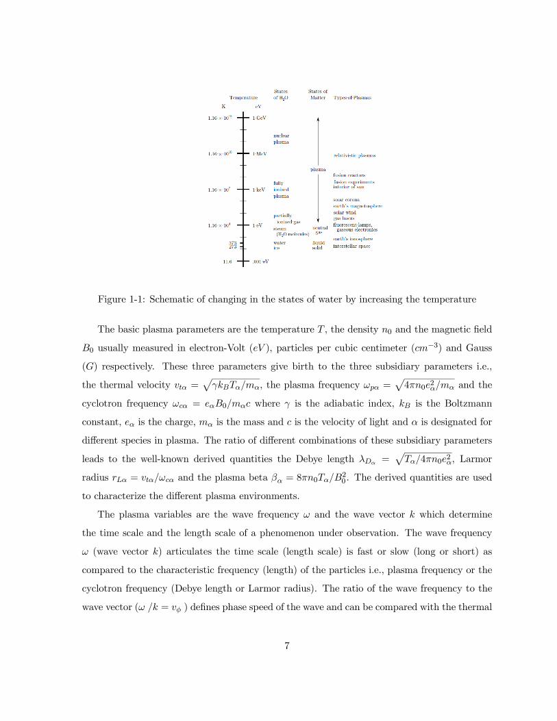
Figure 1-1: Schematic of changing in the states of water by increasing the temperature

The basic plasma parameters are the temperature T , the density n0 and the magnetic field

B0 usually measured in electron-Volt (eV ), particles per cubic centimeter (cm−3) and Gauss

(G) respectively. These three parameters give birth to the three subsidiary parameters i.e.,

the thermal velocity vtα =

γkBTα/mα, the plasma frequency ωpα =

4πn0e2α/mα and the

cyclotron frequency ωcα = eαB0/mαc where γ is the adiabatic index, kB is the Boltzmann

constant, eα is the charge, mα is the mass and c is the velocity of light and α is designated for

different species in plasma. The ratio of different combinations of these subsidiary parameters

leads to the well-known derived quantities the Debye length λDα=

Tα/4πn0e2α, Larmor

radius rLα = vtα/ωcα and the plasma beta βα = 8πn0Tα/B20 . The derived quantities are used

to characterize the different plasma environments.

The plasma variables are the wave frequency ω and the wave vector k which determine

the time scale and the length scale of a phenomenon under observation. The wave frequency

ω (wave vector k) articulates the time scale (length scale) is fast or slow (long or short) as

compared to the characteristic frequency (length) of the particles i.e., plasma frequency or the

cyclotron frequency (Debye length or Larmor radius). The ratio of the wave frequency to the

wave vector (ω /k = vφ ) defines phase speed of the wave and can be compared with the thermal

7

speed vtα of particular species to analyze the dispersion characteristics of the wave.

1.2 Magnetically Confined Plasma

The demand of the worldwide energy is increasing day by day. Saving energy and using re-

newable energy sources are not enough to fulfill this increasing demand. Nuclear energy on the

other hand is obtained by two types of processes i.e., fission and fusion. The fission is a process

in which the energy is produced when the heavy elements like uranium break-up and the fusion

gives energy when the lights elements like deuterium and tritium merge together . The topic

of interest for this thesis is fusion since controlled fusion becomes more realistic.

The fusion is also divided into two categories called inertial confinement fusion (ICF) and

the magnetically confined fusion (MCF). In former approach, the confinement of the plasma

is achieved by making use of petta-watt laser with energy greater than 10MJ to irradiate,

uniformly, a solidified micro target of spherical shape while the latter approach deals with

the confinement due to the very strong magnetic field generated by the superconductor coils.

Both approaches tend to satisfy the Lawson criterion differently i.e., in MCF approach, the

confinement is achieved for long time but low densities whereas ICF confines the plasma for

short time at extremely high densities. The table below depicts the comparison of parameters

for these two types of confinement.

MCF ICF

Particle Density ne 1014cm−3 1026cm−3

Confinement time τ 10 s 10−11s

Lawson criterion neτ 1015scm−3 1016scm−3

As described above that the in MCF approach, the suitable magnetic field configuration

can confine the all charged particles in plasma. A magnetic device, which is called tokamak,

containing a vacuum is used to do so in which mixed tritium and deuterium are inserted. The

schematic picture of tokamak with the magnetic configuration is shown Fig (1.2) portraying

the poloidal and toroidal magnetic fields configuration by passing the current in the coils and

the net magnetic field. The contact of plasma with the walls is avoided due its high temper-

ature requirement by restricting the movement of the particles perpendicular to the field lines

8

Figure 1-2: Schematic of Tokamak

but allowing free movements in the longitudinal direction. Thus the suitable magnetic field

configuration leads to motion of the particles in closed orbits and never escapes.

The design and operation of the Spherical tokamaks are very similar to the tokamaks but

the aspect ratios of both machines are the actual difference where the aspect ratio is the ratio

of the major and minor radii. This ratio for the tokamaks is about between 3 to 5 whereas for

spherical tokamak it is less than 1.5. This less aspect ratio allows spherical tokamaks to operate

at high value of the magnetic pressures that leads to achieve the better confinement. Now a

days, there are running two or more experiments on the spherical tokamaks in Culham, UK ,

New Jersey, USA and Saint Petersburg, Russia the name of the devices are the Mega-Ampere

Spherical Tokamak (MAST), the National Spherical Tokamak Experiment (NSTX) and the

Globus-M tokamak respectively.

1.2.1 Toroidal Geometry

The axisymmetric tokamak geometry can be visualized as simple (quasi-) toroidal coordinates

r, θ, ς, where r is the minor radius, θ and ς are poloidal and toroidal angles [3]. As shown in

9

Figure 1-3: (a) The Toroidal Geometry (b) flux surfaces

Fig.(1.3 a,b) to specify the position on the coordinate surface, one should find the intersection

of two curves from each grid at coordinate surface, r = constant. The property of the curves

of the grid is that any two curves of same family never intersect each other but each curve

from one family crosses the every curve of other family precisely at one point. Thus on the

toroidal surfaces, the every point is labeled as θ + 2πm and ς + 2πn where m and n are

called the toroidal and poloidal mode numbers. The safety factor parameter q(r) is defined as

q(r) ≡ r/R(Bς/Bθ(r)) i.e., the ratio of poloidal magnetic field Bθ(r) and the toroidal magnetic

field Bς(r = 0) where r and R are the minor and major radii respectively. The safety factor

gives the qualitative analysis about the stability of plasma in tokamaks that how many numbers

of toroidal rotations are necessary for a single poloidal rotation of magnetic field line. The value

of the safety factor at the edge of the plasma is qmin(r) > 2− 3. The magnetic field, in the low

pressure plasma where the magnetic surfaces are supposed to be concentric, is

B =Bςeς +Bθeθ

1 + ǫcosθ(1.1)

where eς , eθ are the unit vectors in poloidal and toroidal directions and ǫ = r/R is the inverse

aspect ratio.

10

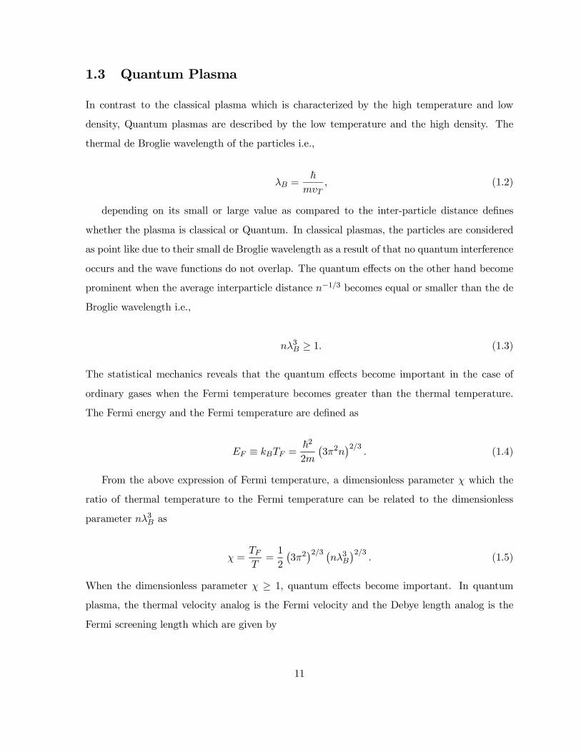
1.3 Quantum Plasma

In contrast to the classical plasma which is characterized by the high temperature and low

density, Quantum plasmas are described by the low temperature and the high density. The

thermal de Broglie wavelength of the particles i.e.,

λB =

mvT, (1.2)

depending on its small or large value as compared to the inter-particle distance defines

whether the plasma is classical or Quantum. In classical plasmas, the particles are considered

as point like due to their small de Broglie wavelength as a result of that no quantum interference

occurs and the wave functions do not overlap. The quantum effects on the other hand become

prominent when the average interparticle distance n−1/3 becomes equal or smaller than the de

Broglie wavelength i.e.,

nλ3B ≥ 1. (1.3)

The statistical mechanics reveals that the quantum effects become important in the case of

ordinary gases when the Fermi temperature becomes greater than the thermal temperature.

The Fermi energy and the Fermi temperature are defined as

EF ≡ kBTF =2

2m

3π2n

2/3. (1.4)

From the above expression of Fermi temperature, a dimensionless parameter χ which the

ratio of thermal temperature to the Fermi temperature can be related to the dimensionless

parameter nλ3B as

χ =TFT

=1

2

3π2

2/3 nλ3B

2/3. (1.5)

When the dimensionless parameter χ ≥ 1, quantum effects become important. In quantum

plasma, the thermal velocity analog is the Fermi velocity and the Debye length analog is the

Fermi screening length which are given by

11

vF =

2kBTF/m =

m

3π2n

1/3(1.6)

λF =vFωp

. (1.7)

Quantum plasmas have attracted much attention due to their applications in electronic

devices having ultra-small size [4], laser plasmas [5] and dense astrophysical plasmas [6]-[8].

Recent developments in quantum plasmas include quantum beam instabilities modification

with quantum corrections [9]-[12], quantum drift waves [13], quantum ion-acoustic waves [14],

Debye screening modifications with magnetic fields for quantum plasmas [15] etc.

1.4 Geodesic Acoustic Modes (GAMs)

Geodesic Acoustic Modes (GAMs) are linear eigen-modes of poloidal plasma rotation supported

by plasma compressibility in toroidal geometry and were first predicted by Winsor et al., [16].

GAMs couple to the drift waves linearly via the toroidal side bands of the plasma perturbations

([16]-[20]) and contain the anisotropic pressure perturbations. The different types of geodesic

oscillations with the wide range of frequencies are observed in different tokamaks ([21]-[24]) and

also in stellarators [25].

The different theoretical models predict different forms of dispersion relation for GAMs

asuuming that any perturbation quantity χ is assumed the form χ = χm exp(−imθ + inζ −iωt)+χm±1 exp(i(m±1)θ+inζ−iωt). The ideal Magnetohydrodynamic (MHD) used by Winsor

et al., [16] results in ωGAM = (

2γ(Te + Ti)/mi)/R where γ represents the ratio of specific

heat for same response of electron and ions and R is the major radius. The two fluid model due

to different response of electrons and ions gives different coefficients of Te and Ti [26]. When

the kinetic theory is used, the dispersion relation becomes ωGAM = (

2(Te + 7Ti/4)/mi)/R.

Smolyakov et al., [27] by including the effect of anisotropy of plasma pressure through the

parallel viscosity tensor, retrieved the same result of kinetic theory from MHD model. The

standard GAM involves m = n = 0 for electric field φ0 and the m = 1 component of plasma

density perturbations i.e., n±1. However when we take finite m and n, the GAM gets modified

12

by Alfven wave as

ω2GAM =7

4

v2tiR2

+ k20v2A ; k0 =

m− nq

R. (1.8)

In the same letter, they also show the electromagnetic dispersion relation of GAMs with different

polarizations and their coupling to Alfven branch as

ω2GAM =21

8

v2tiR2

+v2A

q2R2, (1.9)

and

ω2GAM =7

8

v2tiR2

+v2A

q2R2. (1.10)

1.5 Jeans Instability

The galaxy consists of giant molecular clouds which remain stable due to balance between the

self-gravity and the pressure due to finite temperature. When there is a misbalance between

the inward pressure of gas and the gravity, the collapse of interstellar clouds occurs and the

star formation happens and the perturbation grows exponentially. This is so called the Jeans

instability on the name of Sir James Jeans. The perturbation theory for electrostatic waves

gives the dispersion relation of sound waves as

ω2 = k2v2s , (1.11)

showing that the sound wave is non-dispersive. As the effect of gravity is included the dispersion

relation modifies to

ω2 = k2v2s − ω2J ; ω2J = 4πGρ0, (1.12)

and the dispersion effects enter in the sound wave. However if we compare the above dispersion

relation to the dispersion relation of electron plasma waves

ω2 = k2v2te + 4πn0e2/me, (1.13)

the main difference between Eqs.(1.12, 1.13) resides in the sign that the plasma waves are always

stable but the Eq.(1.12) shows that it becomes purely growing if the last term becomes bigger

13

than the first term and we obtain the growth rate of Jeans instability as

γ =

ω2J − k2v2s , (1.14)

in which the gravitational effects are greater than the inward pressure.

The presence of charged dust grains is the most important phenomenon in astrophysical

situations. It is believed that the dust being the prominent constituent of cosmic environment

and may explain the different type of processes in the astrophysical compact objects. The self-

gravitational instability in the dusty plasma has been discussed by many authors in the recent

years and the new criteria about this instability was obtained. In particular, Salimullah et al.,

[28] discussed the Jeans instability for dust lower hybrid case and also include the quantum

effect through Bohm potential as

γ =

ω2Jd −ω2dlhfi

−ω2Qd4

, (1.15)

where

ω2Jd = 4πGρd , ω2dlh =ωpdωciωpi

, fi = 1−ω2Qd4ω2dlh

; ω2Qd =2k4

m2d

In this thesis, we will extend the work of Ref. [28] with modification due to the drift effects

i.e., the density gradient and the magnetic field gradient.

1.6 Types of Drifts in Plasmas

The intuitive and quite accurate analytic solutions of the velocity (drift) of charged particles can

be determined in arbitrarily complicated electric and magnetic fields which are slowly changing

in both space and time. Drift solutions are obtained by solving the Lorentz equation

mα∂vα∂t

= qα (E+ vα ×B) . (1.16)

The magnitude of this steady drift is easily calculated by assuming the existence of a constant

perpendicular drift velocity in the Lorentz equation, and then averaging out the cyclotron

14

motion:

E+ vα ×B = 0. (1.17)

Taking cross product of above equation with B, we get

VE = vα =E×BB2

. (1.18)

This is called "E-cross-B" drift. The general force drift velocity can easily be derived from

E ×B drift by simply making the replacement E → F/q in the Lorentz equation as

VFα =Fα ×BqαB2

. (1.19)

Comparison of the Equations 1.18 and 1.19 leads to two important conclusions. One is that

a bulk motion, with the velocity VE, of the entire plasma across the magnetic field occurs due

to the electric field which is perpendicular to the magnetic field but does not drive currents in a

plasma. On the other hand, a cross field current is driven by the force (i.e., gravity, centrifugal

force, etc.) perpendicular to magnetic field due to the motion of charged particles (electrons

and ions) in opposite directions.

1.6.1 Non-uniform B Field Drift

For uniform magnetic field, the exact expressions for the drift velocity are derived above however

for the inhomogeneous magnetic field, with respect to space or/and time, the orbit theory is

used. In orbit theory, the ratio of Lamor radius rLα(= v⊥mα/ |qα|B) to the scale length of

homogeneity i.e., rL/L is assumed to be small and expanded.

Grad-B Drift

For case when the field lines are straight but the density changes. The gradient in the magnetic

field then leads to the variation in the Larmor radius i.e., Larmor radius will decrease as

magnetic field strength will increase and vice versa. The grad-B drift is perpendicular to both

the B and ∇B and is proportional to the rL/L and v⊥[29] is given by

15

V∇B = ±1

2v⊥rLα

B×∇B

B2. (1.20)

The coefficient 1/2 comes from average and the ± is the sign of charge showing that the grad-B

drift is in opposite directions for electrons and ions and causes a current perpendicular to the

magnetic field.

Curvature Drift

Considering the case when the magnetic field lines are curve with the constant radius of cur-

vature Rc and the magnitude of magnetic field does not vary. The particles feel, while moving

with random velocity v2 along the magnetic field, the centrifugal force as given by

Fcf =mv2Rc

r =mv2R2c

Rc, (1.21)

and corresponding drift velocity becomes

VR =mαv2qαB2

Rc ×BR2c

. (1.22)

When the magnetic field lines are curve and the magnitude is also varying, like in the case

of tokamak plasma, both the grad B drift and the curvature drifts is added and given the total

drift of the particles as

VR =mα

qα

Rc ×BB2R2c

v2 +

v2⊥2

. (1.23)

1.6.2 Diamagnetic Drift

If the plasma is non-uniform due to gradient either in density or temperature or in both, the

drift velocity may be rewritten by replacing the general force with the pressure force −∇P =

−∇(nγkBT ) as

Vdia,α =B×∇PαnαqαB2

. (1.24)

This drift does not appear in single particle theory and describes the collective behavior

of plasma due to the reason that this drift involves the pressure, an average variable of the

16

plasma, obtained by taking the moment of the distribution. Both the density gradient and the

temperature gradient give rise to non-zero average transverse velocity. Due to diamagnetic drift

an effective drift current flows in the plasma as the motion of the different charged fluids are in

opposite directions to each other.

1.7 Theoretical Model

In this thesis, the different theoretical models are used to study the drift effects on plasma

waves which are given below.

1.7.1 Vlasov Equation

Each particle at any given time has a specific position and velocity. We can therefore charac-

terize the instantaneous configuration of a large number of particles by specifying the density

of particles at each point (x, v) in phase-space. The distribution function for α-species denoted

by fα(x,v, t) prescribes the instantaneous density of particles in phase-space. The number of

particles becomes fα(x,v, t)dxdv at time t having positions and velocities in the range between

x and x+ dx and v and v+ dv respectively. Thus the rate of change of the number of particles

gives the three dimensional Vlasov equation

dfαdt

=∂fα∂t

+ v · ∂fα∂x

+ a · ∂fα∂v

= 0, (1.25)

where the acceleration a from Lorentz force takes the form a =(eα/mα) (E+ v×B/c).

Thus, the distribution function fα(x,v, t) as measured when moving along a particle trajectory

(orbit) is constant. The Vlasov equation is used for collisionless plasma and together with the

Maxwell’s equations

∇.E = 4π

α

ρα , (1.26)

∇.B = 0 , (1.27)

c∇×E = −∂B

∂t, (1.28)

c∇×B =∂E

∂t+ 4π

α

Jα, (1.29)

17

to study the dynamics of electrostatic and electromagnetic plasma systems. When we use

the kinetic theory then the charge and the current densities are expressed as moments of particle

distribution fα as

ρα(x, t) = eα

fα(x,v, t)dv, (1.30)

Jα(x, t) = eα

vfα(x,v, t)dv. (1.31)

The Vlasov equation is a non-linear equation however for this thesis, the focus is only

to linear study of waves in which the field amplitude is sufficiently small. From the Vlasov

equation, the drift kinetic equation and the relativistic Vlasov equation will be formulated.

The drift kinetic equation will further be divided into two regimes i.e., (i) uniform temperature

and density case and (2) non-uniform density and temperature case.

1.7.2 Drift Kinetic Theory

In an electromagnetic field which is varying slowly in time and space, the behavior of a plasma

component can be described by the drift kinetic equation. In Vlasov equation, the distribution

function depends on the velocity vector v whereas the drift kinetic equation is dependent only

on v⊥ and v (and also, certainly, on the coordinates). Thus the drift kinetic equation for the

case of a non-stationary magnetic field and a finite electric field is of the form [30]

∂fα∂t

+∂x

∂t· ∂fα∂x

+∂v∂t

∂fα∂v

+∂v⊥∂t

∂fα∂v⊥

= 0, (1.32)

where

∂x

∂t= e0v +Vd +VE, (1.33)

∂v∂t

=eαmα

E +v2⊥2∇.e0 + vVE .∇e0, (1.34)

∂v⊥∂t

= −vv⊥

2∇.e0 +

v⊥2B

∂B

∂t+VE .∇B

, (1.35)

18

and eα, mα are the charge and the mass of α-species, e0 = B/B with B is the total magnetic

field , E = e0.E is the parallel electric field, Vd = (e0/ωcα)×v2 (e0.∇)e0 +

v2⊥/2

∇ lnB0

is the particle drift velocity due to curvature and inhomogeneity in the magnetic field, VE =

cE×B/B2 is drift velocity called "E×B drift".

Transforming the above drift kinetic equation in terms of energy per unit mass (ε =v2⊥ + v2

/2) and the magnetic moment (µ = v2⊥/2B) and correspondingly rewriting the dis-

tribution function as function of x, t, ε and µ i.e., fα(x, t, ε, µ), we obtain [30]

∂fα∂t

+∂x

∂t·∇fα +

∂ε

∂t

∂fα∂ε

= 0, (1.36)

with

∂x

∂t= e0v +Vd +VE, (1.37)

∂ε

∂t=

eαmα

vE +v2⊥2B

∂B

∂t+VE .∇B

+ v2VE.∇e0, (1.38)

∂µ

∂t= 0. (1.39)

We may linearize the above drift equation (1.36-1.39) to obtain the perturbed distribution

function fα in terms of equilibrium distribution Fα for the large aspect ratio (ǫ = r/R << 1

where r,R are minor and major radii ) systems by assuming magnetic field B = B0(1− ǫ cos θ),

which in turns gives lnB0 = (cos θ er + sin θ eθ), and neglecting the small term B = B.B0/B0

as

dfαdt

+

VE + v

B⊥

B0

.∇Fα +

eαmα

E +

v2⊥2

+ v2

VE .∇ lnB0

∂Fα∂ε

= 0, (1.40)

with making use of the following relations

19

d

dt=

∂

∂t+ v∇ +Vd.∇, (1.41)

Vd =

v2⊥2

+ v2

e0 ×∇ lnB0

ωcα, (1.42)

∇.VE = −2VE .∇ lnB0, (1.43)

e0.∇VE = −VE.∇e0 = −2VE .∇ lnB0. (1.44)

It is also convenient to write down the perturbed electric field, magnetic field and the current

density in terms of scalar potential φ and/or vector potential as

E = −∇φ− 1

c

∂A

∂t, B =∇×

Ab

and J =c

4π∇2⊥A, (1.45)

where b = e0 is the unit vector along the magnetic field. Due to considering the perturbations

with finite m and n numbers, the parallel wave-vector for the principal component and the side

bands are defined as k0 = (m− nq)/qR and k± = (m± 1− n)/qR respectively. The principal

component is assumed to be resonant inside the plasma column and considered mode dynamics

sufficiently close to the rational surface so that k± > k0.

1.7.3 Linear Drift Kinetic Equation for Homogenous Plasma Temperature

and Density

For homogeneous plasma temperature and the density, the second term in Eq.(1.40) vanishes

and the drift equation with the use of the relations in Eqs.(1.41-1.45) take the form[31]

fα = −eαφ

TαFα + gα, (1.46)

where the g distribution function satisfies the equation

ω − ωdα − kv

gα = ωJ20 (zα) (φ−

vcA)

eαFαTα

. (1.47)

20

Here

ωdα = −v2⊥/2 + v2

ωcα

krR

sin θ = − ωdα sin θ, ωdα = ωdαv2⊥/2 + v2

v2tα,

ωdα =krv

2tα

Rωcα, ωcα =

eαB0mαc

, v2tα =2Tαmα

and zα =krv⊥ωcα

.

1.7.4 Linear Drift Kinetic Equation for Inhomogeneous Plasma Temperature

and Density

Adopting the similar procedure as for the homogeneous case, the drift kinetic equation for the

inhomogeneous plasma temperature and density becomes

fα = −eαφ

TαFMα + gα, (1.48)

and the g distribution function (1.47) is modified as

ω − ωdα − kv

gα = J20 (zα)

ω − ω∗α

∂

∂θ

(φ−

vcA)

eαFMα

Tα. (1.49)

where all other quantities are similar as define in Eq.(1.47) except

ω∗α = ω∗α

1 + ηα

v2

v2tα− 3

2

; ω∗α =

cTαN ′0α

eαN0αB0r=

v2tα2Lnαωcαr

ηα = Ln/LT with scale lengths Ln = d lnN/dr and LT = d lnTα/dr.

1.7.5 Two Fluid Ideal MHD Model

The set of equations for ions and electrons including the effect of viscosity is given by

∂n

∂t+∇. (nVE) = 0, (1.50)

3

2

dp

dt+ v.∇p

+

5

2p∇.v+∇.q = 0, (1.51)

dπdt

+ p

−2v.∇ lnB − 2

3∇.v

+

2

5

−2q.∇ lnB − 2

3∇.q

= 0, (1.52)

mndv

dt+∇p+∇.π − eαn(E+ v×B) = 0. (1.53)

21

In above ideal MHD model, we note that the Eq. (1.50) is related to mass conservation,

Eq. (1.51) is for energy conservation and Eq. (1.53) represents momentum conservation. q is

used for the heat flux and π is the parallel component of viscosity tensor π as derived in Ref.

[32].

This model has been used for homogeneous plasma temperature and density by Smolyakov et

al., [27] to explained discrepancy between the results of kinetic and fluid calculations. However

in this thesis, this model is used to explain the discrepancy between the results of kinetic and

fluid calculations for inhomogeneous plasma temperature and the density.

1.7.6 Quantum Magnetohydrodynamic Model

The quantum magnetohydrodynamic model including the effect of gravitational force is given

by [28]

mαnα

∂vα∂t

+ (vα.∇)vα

= nαqα

E+

1

cvα ×B

−∇PT −∇PF

+nα

2

2mα∇

∇2√nα√nα

−mαnα∇ψ, (1.54)

and∂nα∂t

+∇ . (nαvα) = 0. (1.55)

Poisson’s equations for the electrostatic potential φ and gravitational potential ψ are

∇2φ = −4π

α

qαnα and ∇2ψ = 4πGmαnα respectively. (1.56)

Salimullah et al., [28] used this model to study the homogeneous plasma case. However in

this thesis, the above model will be used for inhomogeneous plasma to study the electrostatic

self-gravitational drift waves for magnetized electron-ion-dust plasma (i.e., α = e, i, d ).

1.7.7 Layout

The second chapter includes the effects of density and the temperature inhomogeneities on the

GAMs by using both the drift kinetic equation and the extended magnetohydrodynamic model.

22

By using the full electromagnetic drift equations for electron and ions, the dispersion effects

of Geodesic acoustic mode for m=1 harmonic is discussed in Chapter 3. Chapter 4 contains

the stability analysis of self-gravitational electrostatic drift waves for a streaming nonuniform

quantum dusty magnetoplasma. Summary of Results and discussion is presented in Chapter 5.

Appendixes are given in Chapter 6.

23

Chapter 2

Drift Effects on Geodesic Acoustic

Modes

The full kinetic dispersion relation for the Geodesic acoustic modes(GAMs) including diamag-

netic effects due to inhomogeneous plasma density and temperature is derived by using the drift

kinetic theory. The fluid model including the effects of ion parallel viscosity (pressure anisotropy)

is also presented that allows to recover exactly the adiabatic index obtained in kinetic theory.

We show that diamagnetic effects lead to the positive up-shift of the GAM frequency and ap-

pearance of the second (lower frequency) branch related to the drift frequency. The latter is

a result of modification of the degenerate (zero frequency) zonal flow branch which acquires a

finite frequency or becomes unstable in regions of high temperature gradients.

2.1 Introduction

Geodesic Acoustic Modes (GAMs) [16] is a high frequency branch of Zonal Flow (ZF) and its

role in explaining the suppression of anomalous transport and the turbulence in tokamaks has

been discussed by Diamond et al., [33]. Recently, the several authors studied different aspects

of the GAMs [34]-[36]. The dispersion relation for the high safety factor i.e., q >> 1 takes the

form ωgam = (vti/R)

Γ1 + Γ2/τ +O(q2) where τ = Ti/Te is the temperature ratio of ions to

electrons, the major radius and the ion thermal velocity is represented by R and vti =

2Ti/mi

respectively. The two adiabatic constants (Γ1,Γ2) give different coefficients depending upon the

24

models used. The ideal MHD model for one fluid [16] yielded Γ1 = Γ2 = 5/3. Kinetic models

[34],[35],[18] have predicted Γ1 = 7/4 and Γ2 = 1. Smolyakov et al., [31] showed that in GAMs,

the pressure perturbations exhibit the intrinsically anisotropic behavior and on including this

pressure anisotropy through the parallel component of ion viscosity, both the coefficients for

ideal MHD case becomes exactly similar to the coefficient resulted by the kinetic model.

Standard GAM includes symmetric poloidal perturbation (M = 0) of electrostatic potential

which couples with the poloidal density perturbation of the side-bands (M = ±1). Poloidally

inhomogeneous perturbations effectively couple to gradient driven drift wave turbulence. Beta

Alfvén Eigenmodes (BAEs )[37] are another type of GAMs with finite M = 0 due to the effect

of the gradients in the density and temperature profile. BAE dispersion relations were discussed

in local approximation [17]—[39]and also by means of ballooning theory [18],[40],[41]. GAM and

BAE have similar dispersion relations [35],[42] with the difference residing in the poloidal and

toroidal modes (M = N = 0 for GAM and M,N = 0 for BAE). BAE and related modes have

been studied in a number of papers. In particular, unstable beta induced temperature gradient

(BTG) modes have been found using MHD [38]and kinetic [39] models. Beta-induced Alfvén and

Alfvén-Acoustic Eigenmodes (BAE and BAAE, respectively) have been widely investigated due

to its role in background turbulence, generation of zonal flows and the possibility of application

in MHD spectroscopy to diagnose safety factor profiles, q(r), in tokamaks [36],[22]-[44].

Much work in studies of GAM/BAE was done with kinetic theory, particularly, taking

into account the resonance damping due to Landau mechanism [45],[46]. Yet, the fluid theory

remains an attractive alternative to full kinetic studies, especially, for studies of nonlinear

effects, e.g. nonlinear generation of GAM due to drift wave turbulence [35],[47],[48]. Much of

such work was done in fluid theory and it is desirable to have a fluid theory that self consistently

includes drift effects in both GAM modes as well in the background drift wave turbulence.

This chapter presents both the drift kinetic theory and two fluid MHD theory investigating

the diamagnetic effects on GAM. We provide a simple analytical model for GAM in presence of

diamagnetic effects. We show that in presence of diamagnetic effects, previously degenerated

(zero frequency) mode, normally associated with zonal flow acquires a finite frequency. More-

over, for large gradients of the temperature, the latter mode becomes unstable in the regions

of high q.

25

2.2 Drift Kinetic Equation and Full Kinetic Dispersion Relation

The perturbed distribution function (1.49) for the electrostatic case reduces to

fα = −eαFMTα

φ+ g, (2.1)

and g distribution takes the form

ω − k0v

g0 − ωdαg =

ω − ω∗α

∂

∂θ

φ0J

20 (zα)

eαFMTα

, (2.2)

ω − k0v

g − ωdαg0 − (ωdαg − ωdαg)− kvg =

ω − ω∗α

∂

∂θ

φJ20 (zα)

eαFMTα

, (2.3)

with

ωdα = −v2⊥/2 + v2

ωcα

krR

sin θ = −ωdα sin θ, ω∗α = ω∗α

1 + ηα

v2

v2tα− 3

2

,

ω∗α =cTαN

′0

eαN0B0R=

vtα2Lnωcαr

, ωcα =eαB0mαc

,and zα =k⊥v⊥ωcα

.

Using perturbations of the form for GAMs as

X = X0 +X1eiθ +X−1e

−iθ = X0 +X1c cos θ + iX1s sin θ, (2.4)

Eq. (2.2) becomesω − k0v

g0 +

iωdα2

g1s = ωφ0J20 (zα)

eαFMTα

, (2.5)

and after separating the different parities (g1 + g−1) and (g1 − g−1), Eq. (2.3) takes the form

ω − k0v

(g1c)−

vqR

(g1s) = [ωφ1c − ω∗αφ1s] J20 (zα)

eαFMTα

, (2.6)

and

−vqR

g1c +ω − k0v

g1s − iωdαg0 = [ωφ1s − ω∗αφ1c]J

20 (zα)

eαFMTα

, (2.7)

where we have used

ωdαg = −iωdα2

g1s,

26

and introduced the notations X1c,s = X1 ±X−1.

The solutions of Eqs. (2.4-2.6) enable to find the distribution function g

g0 = −J20 (zα)

eαFMTα

W

iωdαω

2

φ1s −

ω∗αω

φ1c

+

iωdαv2qR

φ1c −

ω∗αω

φ1s

−ω2 −

v2q2R2

φ0

, (2.8)

g1c = −J20 (zα)

eαFMTα

W

−ω2 − ω2

dα

2

φ1c −

ω∗αω

φ1s

−

vω

qR

φ1s −

ω∗αω

φ1c

−iωdαvqR

φ0

, (2.9)

g1s = −J20 (zα)

eαFMTα

W

−ω2

φ1s −

ω∗αω

φ1c

−

vω

qR

φ1c −

ω∗αω

φ1s

− iωωdαφ0

, (2.10)

and resultantly, the perturbed distribution functions of principal and side-band component

become

f0 = −eαFMα

Tα

φ0 +

J20 (zα)

W

iωdαω

2

φ1s −

ω∗αω

φ1c

+

iωdαv2qR

φ1c −

ω∗αω

φ1s

−ω2 −

v2

q2R2

φ0

,

(2.11)

f1c = −eαFMα

Tα

φ1c +

J20 (zα)

W

−ω2 − ω2

dα

2

φ1c −

ω∗αω

φ1s

−

vω

qR

φ1s −

ω∗αω

φ1c

−iωdαvqR

φ0

,

(2.12)

f1s = −eαFMα

Tα

φ1s +

J20 (zα)

W

−ω2

φ1s −

ω∗αω

φ1c

−

vω

qR

φ1c −

ω∗αω

φ1s

− iωωdαφ0

,

(2.13)

where

W = ω2 −v2

q2R2− ω2dα

2.

2.2.1 Density Perturbations

Now we calculate the density perturbation from the moment of the perturbed distribution as

nα =

fαd

3v. (2.14)

27

By using the Eqs. (2.11-2.13) in above equation, we get

n0α = −eαN0αTα

1− Γ0α −

ω2dα2ω2

I20α

φ0 +

i

2

ωdαω

I10α φ1s −

ω∗αω

I10∗αφ1c

, (2.15)

n1c = −eαN0αTα

1− I00α − ω2dα

2ω2I20α

φ1c +

ω∗αω

I00∗α −

ω2dα2ω2

I20∗α

φ1s

, (2.16)

n1s = −eαN0αTα

1− I00α

φ1s +

ω∗αω

I00∗αφ1c − iωdαω

I10α φ0

. (2.17)

The all the integrals are given in the Appendix. A.

2.2.2 Quasi-neutrality condition

The quasi-neutrality condition ( i.e., ne−ni = 0) for each component of the density perturbation

leads to the following set of equations

S01φ0 −i

2

ωdiω

S03φ1s +i

2

ωdiω

ω∗iω

S∗03φ1c = 0, (2.18)

φ1c −ω∗iω

S∗00S00

φ1s = 0, (2.19)

S′00φ1s +ω∗iω

S′∗00φ1c − iωdiω

S03φ0 = 0, (2.20)

with the auxiliary coefficients as

S00 =

1− I00i − ω2di

2ω2I20i

+ τ−1

1− I00e − ω2de

2ω2I20e

,

S∗00 = I00∗i −ω2di2ω2

I20i −I00∗e −

ω2de2ω2

I20∗e

,

S′00 =1− I00i

+ τ−1

1− I00e

,

S′∗00 = I00∗i − I00∗e ,

S01 = Γ0i − 1 +ω2di2ω2

I20i + τ−1Γ0e − 1 +

ω2de2ω2

I20e

,

S03 =I10i − I10e

,

S∗03 =

I10∗i +

ω∗eω∗i

I10∗e

.

28

2.2.3 Dispersion relation

Using above Eq. (2.19) in Eq. (2.20), we obtain

φ1s = iωdiω

S03S00

S′00S00 +ω2∗iω2

S′∗00S∗00φ0, (2.21)

and substituting Eq. (2.21) in Eq. (2.20), we get

φ1c = iωdiω

ω∗iω

S03S∗00

S′00S00 +ω2∗iω2

S′∗00S∗00φ0. (2.22)

Solving Eq. (2.18) with the help of Eqs. (2.21, 2.22), the dispersion relation becomes

S01 +ω2di2ω2

S03

S03S00 −

ω2∗iω2

S∗03S∗00

S′00S00 +ω2∗iω2

S′∗00S∗00= 0 (2.23)

The above dispersion relation is the full kinetic dispersion relation of electrostatic GAMs which

includes the effects of both the temperature and density inhomgeneities, the Landau and toroidal

resonances.

2.2.4 Simplified Dispersion Relations

Assuming that ions are in the fluid regime (ω >> vti/qR0), and the electrons are in the

adiabatic regime (ω << vte/qR0), the general integrals in Appendix A may be expanded as

given in Appendixes. (B, C) and resultantly we obtain

ω2 − v2tiR20

7

4+

τ + (1 + ηi)ω2∗/ω

2

τ2 − (ω2∗/ω2)

= 0. (2.24)

2.3 Two Fluid MHD Model

In the study of GAM, it is reasonable to assume that ions are in the fluid regime, ω >>

vti/qR0, and the electrons are in the adiabatic regime, ω << vte/qR0. In this context, electron

temperature fluctuations can be neglected in the lowest order and the electron has a Boltzmann

response as consequence. On the other hand, for ions, parallel viscosity, π =3π(bb− I/3)/2,

29

must be consider to account for pressure anisotropy (π = 2(p − p⊥)/3) effects.

In this chapter, we use ideal MHD equations for ion and electrons in the form:

∂n

∂t+∇. (nVE) = 0, (2.25)

3

2

dp

dt+ v.∇p

+

5

2p∇.v+∇.q = 0, (2.26)

dπdt

+ p

−2v.∇ lnB − 2

3∇.v

+

2

5

−2q.∇ lnB − 2

3∇.q

= 0, (2.27)

mndv

dt+∇p+∇.π − eαn(E+ v×B) = 0, (2.28)

We note that Eqs. (2.25, 2.26, 2.28), representing conservation of mass, energy and momentum

respectively, have been widely used in both one and two fluid models. Eq. (2.27) is the parallel

component of Grad type equation for the viscosity tensor, π, that was derived for general

curvilinear magnetic field in Ref. [32]. Parallel velocity, v, which is responsible for O(q2)

corrections, is neglected in our analysis since GAM is mostly important at the edge of the

plasma column.

Taking the cross product of Eq. (2.28) withB/B = b, one finds the equation for ion/electron

currents

J = JI + Jp + Jπ + J + eαnVE , (2.29)

where

JI =eαn

ωcα

b×dv

dt

,Jp =

b×∇p

B,Jπ =

b×∇.π

B, J = Jb,

VE =b×∇φ

Band E = −∇φ−

∂A∂θ

b.

Eqs. (2.25- 2.29) are closed with quasi-neutrality condition in the forms

e(ni − ne) = 0, ∇.J = 0. (2.30)

Here, the subscript α = e, i, standing for ions and electrons species, were omitted in n, v, p, q,

30

m and π for simplicity of notation. As in standard ideal MHD models, frozen field condition

E+ v×B = 0, (2.31)

from Eq. (2.28), is considered to find the velocity in a first approximation [27]. The velocity,

VE , is then used in the continuity equation for ions

∂ni∂t

+VE .∇n0 + n0∇.VE = 0, (2.32)

to find the first side-bands components of ion density, ni±1. Here the second term is responsible

for the density drift effects. The following perturbed quantities, φ, n, p, π, are assumed to be

in the form

X = X0 +X1 exp(iθ) +X−1 exp(−iθ), (2.33)

since for the study of GAM only poloidal modes M = 0,±1 and the toroidal mode N = 0 are

important. Then, by using (2.33) into (2.32) we obtain

ni±1 =

± i

2

ωdiω

φ0 ∓ω∗ω

φ±1

, (2.34)

where ωdi = krρivti/R0 is the magnetic drift frequency, ω∗ = ω∗i is the density drift frequency

defined by ω∗i = Tin′0/ (reB0n0) = ρivti/ (2rLN) and LN = (d lnn0/dr)

−1 is the characteristic

density scale length. To solve (2.32) we use∇.VE = −2VE.∇ lnB and we consider high aspect

ratio approximation, ǫ = r/R0 << 1, and circular magnetic surfaces tokamaks, which gives B

≈ B0(1− ǫ cos θ) and consequently ∇ lnB = (− cos θer + sin θeθ)/R0.

For electrons, due to its small mass, the parallel component of the momentum equation can

be approximated by

Te∇ne − en0∇φ = 0, (2.35)

which leads to the Boltzmann response as solution for the first side-bands,

ne±1 =en0Te

φ±1. (2.36)

By substituting (2.34) and (2.36) in the quasi-neutrality condition, e(ni − ne) = 0, we obtain

31

the relation between the potentials,

φ±1 = ± i

2

ωdi/ω

τ ± ω∗/ωφ0, (2.37)

in according with Refs. [39], [49] (Eqs. (8) and (3.8), respectively) using kinetic model. Here

the ratio of temperatures is τ = Ti/Te.

The reduced energy equation for ions is obtained in the form

3

2

dpidt

+VE .∇p0i

+

5

2p0i∇.VE = 0. (2.38)

It is solved for the first side-bands of ion pressure,

pi±1 =

±5

3

i

2

ωdiω

φ0 ∓ (1 + ηi)ω∗ωφ±1

en0, (2.39)

where ηi = Ln/LT and d lnT/dr is the characteristic ion temperature scale length. It is worth

noting here that, in general, the heat flux (q), nor the diamagnetic drift, are not divergence

free in toroidal geometry. It can be shown however, that these effects do not contribute to the

GAM dispersion in the leading order.

In case of electrons, since fluctuations of temperature are small in the adiabatic regime,

electron pressure can be written as

pe±1 = ±φ±1en0. (2.40)

From the reduced ion parallel viscosity equation [27]

dπidt

− 2

3poiVE .∇ lnB = 0, (2.41)

in which heat flux contributions can be neglected, we obtain the first side-bands of parallel

viscosity

πi±1 = ± i

6

ωdiω

φ0en0, (2.42)

where it can be noted that this equation is unchanged by diamagnetic effects.

Considering that electrons are isotropic and so πe = 0, it is convenient to compute the sin θ

32

component of the combination p+ π from both ions and electrons contribution

(p+ π/4)s = −ωdiω

7

4+

τ + (1 + ηi)ω2∗/ω

2

τ2 − (ω2∗/ω2)

φ0en0. (2.43)

This will be used in the current conservation equation averaged over the magnetic surfaces

∇.J = 0, (2.44)

where J is the sum of the ion and electron currents and the average over the magnetic surfaces,,is used to eliminate the parallel current contributions, since

∇J

= 0. In Eq. (2.44), since

ωci << ωce and the ion and electron currents due to VE cancel each other, we need to consider

ion inertial current, the total (ion and electron) diamagnetic current, and the viscosity current

for ions.

The divergence of these currents averaged over the magnetic surfaces are calculated in the

leading order as follows:

∇.JI ≈en0ωcib×dVE

dt

≈iωen0ωci

∇.∇⊥φ

B

≈ −4π2rR0iω

en0ωci

k2r φ0B0

, (2.45)

∇.Jp +∇.Jπ ≈ −2Jp.∇ lnB + Jπ.∇ lnB ≈−2ikrp sin θ

R0B0−

ikrπ sin θ

2R0B0

,

≈ −4π2rR0ikr (p+ π/4)s

R0B0. (2.46)

Finally, the dispersion relation can then be written in the form

ω2 − v2tiR20

7

4+

τ + (1 + ηi)ω2∗/ω

2

τ2 − (ω2∗/ω2)

= 0. (2.47)

This equation has following solutions:

2Ω2± = ω2gam + ω2∗e ±

ω2gam + ω2∗e2

+ (4ηi − 3)ω2∗ev2ti/R

20. (2.48)

where ω2∗i = −ω2∗e/τ is the electron drift frequency and ω2gam = (7/4 + 1/τ)v2ti/R20 is the GAM

frequency in the absence of drift effects.

It can be seen from this equation, that diamagnetic effects due to temperature and density

33

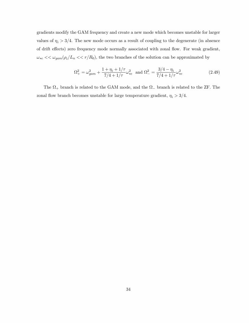
gradients modify the GAM frequency and create a new mode which becomes unstable for larger

values of ηi > 3/4. The new mode occurs as a result of coupling to the degenerate (in absence

of drift effects) zero frequency mode normally associated with zonal flow. For weak gradient,

ω∗e << ωgam(ρi/Ln << r/R0), the two branches of the solution can be approximated by

Ω2+ = ω2gam +1 + ηi + 1/τ

7/4 + 1/τω2∗e and Ω2− =

3/4− ηi7/4 + 1/τ

ω2∗e (2.49)

The Ω+ branch is related to the GAM mode, and the Ω− branch is related to the ZF. The

zonal flow branch becomes unstable for large temperature gradient, ηi > 3/4.

34

Chapter 3

Electromagnetic Effects on Geodesic

Acoustic Modes

By using the full electromagnetic drift kinetic equations for electrons and ions, the general dis-

persion relation for geodesic acoustic modes (GAMs) is derived incorporating the electromag-

netic effects. It is shown that m=1 harmonic of the GAM mode has a finite electromagnetic

component. The electromagnetic corrections appear for finite values of the radial wave numbers

and modify the GAM frequency. The effects of plasma pressure βe, the safety factor q and the

temperature ratio τ on GAM dispersion are analyzed.

3.1 Introduction

Geodesic Acoustic Modes (GAMs) are linear eigenmodes of poloidal plasma rotation supported

by plasma compressibility in toroidal geometry and were first predicted by Winsor et al., [16].

They are closely related to Beta-induced Alfvén eigenmodes (BAEs) [17, 18, 44, 55, 56]. Geo-

desic Acoustic Modes have attracted much interest both experimentally and theoretically due

to their possible role in drift-wave turbulence and plasma transport. The coupling of GAMs,

zonal flows, and small scale drift-wave fluctuations via toroidal effects and nonlinear Reynolds

stress has been noted in a number of simulations [57]-[59]. The fluctuations with GAM signa-

tures and in the GAM frequency range have been observed in numerous devices [51], [61]-[63].

It has been suggested that GAMs can be used also for magnetohydrodynamic spectroscopy and

35

diagnostics of the current profile in burning plasmas [64, 65].

The kinetic aspects of GAM modes have been investigated theoretically by several authors

[68]-[70]. One of the important issue is the mode dispersion which determines the radial prop-

agation and radial structure of GAMs [68, 71, 72, 62]. It has been shown that the second

sideband harmonics of GAM (which are generally electromagnetic) are important for form-

ing the eigenmode structure in MHD models [56, 66, 67]. Most of kinetic studies so far have

considered electrostatic approximation and neglected the magnetic component of the GAM.

Electromagnetic effects were considered in Refs. [69, 73], however it was concluded [69] that

the magnetic component of the first side bands of GAM is identically zero and therefore only

the second order sidebands can be electromagnetic. The electromagnetic effects of the second

sidebands on the GAM frequency and damping rates were kinetically analyzed in Ref. [73]. It

was noted however [20] that global GAMs with large radial extent should have substantial elec-

tromagnetic component. It is shown in the present paper that for higher plasma pressure, the

first sideband of the perturbed magnetic potential can be of the same order as the electrostatic

sideband and the corresponding expression for the magnetic component is derived.

For the analytical derivation of the dispersion relation, we assume that all perturbations

vary as X = X0 exp+ X±1 exp (±iθ) + X±2 exp (±2iθ) , where X0 and X±1, X±2 represent the

principal and sideband components. Respectively, the wave vectors for the sidebands are k± =

±1/qR, k2± = ±2/qR and the principal harmonic has k0 = (m− nq) /qR =0. In this paper,

we solve the full electromagnetic drift kinetic equations for electrons and ions and obtain the

general dispersion relation for the principal m = n = 0 mode and m = 1 sidebands only. The

general dispersion relation incorporates the effects of the finite value of the parallel wave vector

k± (both for electrons and ions) and radial dispersion due to electromagnetic effects . We

also obtain the simplified dispersion relation by assuming that the electrons are in adiabatic

regime ω < vTe/qR whereas the ions are in the fluid regime ω > vTi/qR. The main finding

of the present work is that the parallel current in the first order is finite resulting in magnetic

nature of the sidebands controlled by the radial mode width parameter K⊥ = ckrλDe/ωqR.

The electromagnetic corrections contribute to the mode dispersion and have to be included in

the dispersive models of GAMs that are required for the determination of the GAM eigenmode

properties. We also show the route for the self-consistent expansion including the second order

36

harmonics. This is further discussed in the Appendix E.

In the followings, we solve the drift kinetic equation and obtain the general kinetic dispersion

relation of GAMs and then by simplifying the electron and ion responses, the dispersion relation

is obtained in the limit when the electrons are in the adiabatic regime (ω < vTe/qR) and the

ions are in the fluid regime(ω > vTi/qR) . At the end, the summary of the results is given.

3.2 Drift Kinetic Equation and Full Kinetic Dispersion Relation

We use the drift kinetic equation in the form

fα = −eαφ

TαFMα + gα, (3.1)

where the g distribution function satisfies the equation

ω − ωdα − kv

gα = ωJ20 (zα) (φ−

v

cA)

eαFMα

Tα. (3.2)

Here

ωdα = −v2⊥/2 + v2

ωcα

krR

sin θ = − ωdα sin θ, ωdα = ωdαv2⊥/2 + v2

v2tα,

ωdα =krv

2tα

Rωcα, ωcα =

eαB0mαc

, v2tα =2Tαmα

and zα =krv⊥ωcα

.

Separating the principal and the oscillating components of Eq. (3.2), we obtain

ωg0α − ωdαgα = ω(φ0 −vcA0)J

20 (zα)

eαFMα

Tα,

(3.3)

ωgα − ωdαg0α − (ωdαgα − ωdαgα)− kvgα = ω(φ−vcA)J20 (zα)

eαFMα

Tα.

(3.4)

The notation ... represents the average in θ. The magnetic vector potential A describes the

electromagnetic effects and leads to the higher order corrections to the density perturbation

and the parallel current.

37

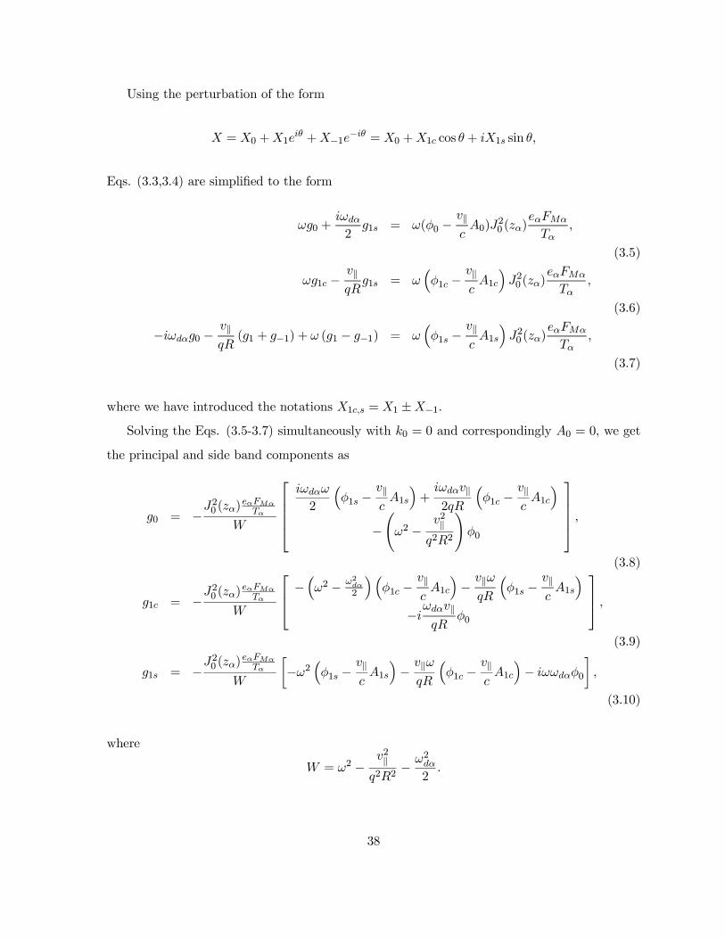
Using the perturbation of the form

X = X0 +X1eiθ +X−1e

−iθ = X0 +X1c cos θ + iX1s sin θ,

Eqs. (3.3,3.4) are simplified to the form

ωg0 +iωdα2

g1s = ω(φ0 −v

cA0)J

20 (zα)

eαFMα

Tα,

(3.5)

ωg1c −vqR

g1s = ωφ1c −

vcA1c

J20 (zα)

eαFMα

Tα,

(3.6)

−iωdαg0 −vqR

(g1 + g−1) + ω (g1 − g−1) = ωφ1s −

v

cA1s

J20 (zα)

eαFMα

Tα,

(3.7)

where we have introduced the notations X1c,s = X1 ±X−1.

Solving the Eqs. (3.5-3.7) simultaneously with k0 = 0 and correspondingly A0 = 0, we get

the principal and side band components as

g0 = −J20 (zα)

eαFMα

Tα

W

iωdαω

2

φ1s −

vcA1s

+

iωdαv2qR

φ1c −

vcA1c

−ω2 −

v2q2R2

φ0

,

(3.8)

g1c = −J20 (zα)

eαFMα

Tα

W

−ω2 − ω2

dα

2

φ1c −

vcA1c−

vω

qR

φ1s −

vcA1s

−iωdαv

qRφ0

,

(3.9)

g1s = −J20 (zα)

eαFMα

Tα

W

−ω2

φ1s −

vcA1s

−

vω

qR

φ1c −

vcA1c

− iωωdαφ0

,

(3.10)

where

W = ω2 −v2

q2R2− ω2dα

2.

38

Using the Eqs. (3.8-3.10) in Eq. (3.1), the perturbed distributions simplify to

f0 = −eαFMα

Tα

φ0 +

J20 (zα)

W

iωdαω

2

φ1s −

vcA1s

+iωdαv2qR

φ1c −

vcA1c

−ω2 −

v2q2R2

φ0

,

(3.11)

f1c = −eαFMα

Tα

φ1c +

J20 (zα)

W

−ω2 − ω2

dα

2

φ1c −

v

cA1c

−vω

qR

φ1s −

v

cA1s

−iωdαvqR

φ0

,

(3.12)

f1s = −eαFMα

Tα

φ1s +

J20 (zα)

W

−ω2φ1s −

vcA1s

−vω

qR

φ1c −

vcA1c

− iωωdαφ0

.

(3.13)

3.2.1 Density Perturbation

Now we calculate the density perturbation

n =

fd3v. (3.14)

Using Eq. (3.11-3.13) in Eq. (3.14), we obtain the following expressions for various compo-

nents of density perturbation

n0α = −eαN0Tα

1− Γ0α −

ω2dα2ω2

I20α

φ0 + i

ωdα2ω

I10α φ1s − iωdα2ω

I11αs2α

ωqR

cA1c

, (3.15)

n1cα = −eαN0Tα

(1− Γ0α)φ1c −

I01αs2α

φ1c −

ωqR

cA1s

, (3.16)

n1sα = −eαN0Tα

1− I00α

φ1s +

I01αs2α

ωqR

cA1c − i

ωdαω

I10α φ0

. (3.17)

The definitions of various integrals are given in Appendix A, and sα = ωqR/vtα. The

39

quasi-neutrality equation together with Eqs. (3.15-3.17) gives

S01φ0 + iωdi2ω

S02ωqR

cA1c −

i

2

ωdiω

S03φ1s = 0, (3.18)

φ1c −

ωqR

cA1s

= −

(Γ0i − 1) + τ−1 (Γ0e − 1)

D1

φ1c, (3.19)

φ1s −

ωqR

cA1c

=

S1D1

φ1s − iωdiω

S03D1

φ0, (3.20)

where we have defined the auxiliary coefficients as follows

S01 = Γ0i − 1 +ω2di2ω2

I20i + τ−1Γ0e − 1 +

ω2de2ω2

I20e

,

S02 =I11is2i− I11e

s2e,

S03 =I10i − I10e

,

S1 = 1− I00i +I01is2i

+ τ−11− I00e +

I01es2e

,

D1 =I01is2i

+ τ−1I01es2e

,

and the temperature ratio as τ = Te/Ti.

3.2.2 Current Density

The perturbed distribution function in Eqs. (3.12,3.13) can be used to calculate the parallel

current perturbation

j = eα

fvd

3v,

so that we obtain

j1cα = −e2αN0αTα

ωqR

Γ0α

s2α+

I02αs4α

ωqR

cA1c −

I01αs2α

φ1s − iωdαω

I11αs2α

φ0

, (3.21)

j1sα =e2αN0αTα

ωqRI01

s2α

φ1c −

ωqR

cA1s

. (3.22)

40

Total parallel current of Eq. (3.21) as a sum of electron and ion contributions becomes

j1c = j1ce + j1ci =e2N0Ti

ωqR

S2

φ1s −

ωqR

cA1c

− [S2 −D1]φ1s + i

ωdiω

S02φ0

, (3.23)

where

S2 =

Γ0i

s2i+

I02is4i

+ τ−1

Γ0e

s2e+

I02es4e

.

Using Eq. (3.20) in Eq. (3.23), the total parallel current can be reduced to the form

j1c =e2N0Ti

ωqR

S1S2D1

− S2 +D1

φ1s − i

ωdiω

S03S2D1

− S02

φ0

. (3.24)

Using the Ampere’s law k2rA1c = 4πc j1c gives the expression for the perturbed vector potential

A1c =τc

K2⊥ωqR

S1S2D1

− S2 +D1

φ1s − i

ωdiω

S03S2D1

− S02

φ0

. (3.25)

The parameter K2⊥, which is responsible for the electromagnetic natures of the GAM [20], is

defined as

K2⊥ =

c2k2rλ2De

ω2q2R2.

Note that for GAM range frequencies ω2 ≃ v2Ti/R2, the K2

⊥ parameter becomes K2⊥ ≃

τk2rc2/q2ω2pi

≃ τk2rρ

2i /βiq

2. Since we are interested only in GAM mode, only the cos θ

parity current is shown here. The sin θ parity can be calculated similarly.

3.2.3 Full Kinetic Dispersion relation

The Eqs. (3.18, 3.20, 3.25) are used to derive the general dispersion relation. After putting Eq.

(3.25) in Eqs. (3.18, 3.20), we get

S01 +

ω2di2ω2

τS202K2⊥

S03S02

S2D1

− 1

φ0 −

i

2

ωdiω

S03 −

τ

K2⊥

S02

S1S2D1

− S2 +D1

φ1s = 0,

(3.26)

41

φ1s = −iωdiω

S03D1

+τS02K2⊥

S03S02

S2D1

− 1

1− τ

K2⊥

S1S2D1

− S2 +D1

− S1

D1

φ0. (3.27)

Solving the above two equations yields

S01 +ω2di2ω2

τ

K2⊥

S202

S03S02

S2D1

− 1

− ω2di2ω2

S202D1

S03S02

+τD1

K2⊥

S03S2S02D1

− 1

1 +

S03S02

− 1 +S1D1

1− τ

K2⊥

S1S2D1

− S2 +D1

− S1

D1

= 0.

(3.28)

The above equation represents the general dispersion relation of GAMs with full kinetic

response of electron and ions including the electromagnetic corrections. The latter depend on

the radial mode width characterized by the K⊥ parameter. The limit of large (small) value

of the parameter K2⊥ > 1

K2⊥ < 1

describes the electrostatic (electromagnetic) behavior of

the sidebands. This equation can be used to investigate the role of electromagnetic effects on

the mode dispersion and mode damping. This equation includes both Landau ω ≃ v/qR and

toroidal ω ≃ ωdα resonances.

3.3 Simplified Dispersion Relation

In this section we derive the simplified dispersion equation by neglecting the resonant effects

i.e., assuming that the electrons are in the adiabatic regime (se < 1) and ions are in the fluids

regime si > 1. We also assume the small Larmor radius limit so that the toroidal resonances can

be neglected as well: ω2de < ω2 and ω2di < ω2. In this limit, the expanded form of the integrals

can be used as given in Appendices (B, C). The simplified dispersion equation can be directly

derived from the full expression (3.28) by using Appendix D, but we give here all simplified

expressions for plasma density and potentials to highlight the nature of the magnetic correction

and estimate its amplitude. In this section we only show the components n1se, φ1s and A1c

42

relevant to GAM polarization [31].

3.3.1 Electron Response

The simplified electron response is obtained from Eqs. (3.15-3.17, 3.21), by using the expansions

given in Appendix B, as

n0e = − i

2

en0Te

ωdeω

ωqR

cA1c, (3.29)

n1ce =en0Te

φ1c −

ωqR

cA1s

, (3.30)

n1se =en0Te

φ1s −

ωqR

cA1c

, (3.31)

j1ce =e2n0Te

ω2q2R2

cA1c − ωqRφ1s + iωdeqRφ0

. (3.32)

These expressions can also be obtained from fluid equations [31]. Expressions (3.30,3.31) follow

from the electron momentum balance equation in the adiabatic limit ω < vTe/qR. The equa-

tions (3.29) and (3.32) can be obtained respectively from the m = 0 and m = 1 components of

the electron continuity equation and using Eqs. (3.30, 3.31).

3.3.2 The Ion Response

Similarly, using the Appendix C, we may simplify the ion equations (3.15-3.17, 3.21) by using

the expansions ω > vTi/qR and ωDi < ω:

n0i =eN0Ti

Γ0i − 1 +

1

2

K2 +K2

φ0 −

i

2

K1 +K1

φ1s +

i

2K1

ωqR

cA1c

,

(3.33)

n1ci = −eN0Ti

φ1c (1− Γ0i)−

φ1c −

ωqR

cA1s

K

,

(3.34)

n1si =eiN0Ti

Γ0i − 1 +K +

1

2K2 +

1

2K2

φ1s −K

ωqR

cA1c + i

K1 +K1

φ0

,

(3.35)

j1ci =e2N0Ti

ωqR

K

φ1s −

ωqR

cA1c

+ iK1φ0

.

(3.36)

43

The terms with Γ0i − 1 are responsible for inertial (polarization) corrections, the terms

with K are due to parallel ion motion (ion sound dynamics), the terms with K1 are due to

toroidal compressibility, and K1 is the combination of the toroidal compressibility and ion

sound dynamics. Note that the full parallel electric field E = −iφ1c −

ωqR

cA1s

/qR, which

includes the electromagnetic part is used to calculate the parallel ion response.

3.3.3 The Dispersion Relation and Magnetic Perturbation Effect

The quasi-neutrality conditions for principal and oscillating components take the form

0 =

Γ0i − 1 +

1

2K2 +

1

2K2

φ0 −

i

2

K1 +K1

φ1s −

ωqR

cA1c

, (3.37)

φ1c −

ωqR

cA1s

=

(Γ0i − 1)τ−1 −K

φ1c, (3.38)

φ1s −

ωqR

cA1c

=

Γ0i − 1 +1

2K2 +

1

2K2

τ−1 −K

φ1s + i

K1 +K1

τ−1 −K

φ0. (3.39)

Total parallel current

j1c = −e2N0Ti

ωqR

φ1s −

ωqR

cA1c

τ−1 −K

− i

K1 +K1

φ0

. (3.40)

Using Eq. (3.39) in above equation, we obtain the parallel current in terms of the cos θ harmonic

of the electrostatic potential

j1c = −ωqRe2N0Ti

(Γ0i − 1 +1

2

K2 +K2

)φ1s. (3.41)

With the Ampere’s law one obtains general expression for the perturbation of the magnetic

vector potential

A1c = − τc

K2⊥ωqR

Γ0i − 1 +

1

2

K2 +K2

φ1s. (3.42)

The expression (3.41) creates the impression that the parallel current is the finite Larmor radius

effects, as it was assumed in Refs. [69, 73]. In fact, the GAM involves the balance of the ion

polarization current and the divergence of the diamagnetic current, so it is in the same order

44

as the magnetic perturbation given by Eq. (3.42). It is easy to see that radial wave vector kr

cancels out from Eq. (3.42).

It is instructive at this point to compare our expressions with those in Refs. [69, 73]. Our

expression for the parallel current j1c in Eq. (3.41) is identical to the fluid limit of the expression

(5) of Ref. [69]. We believe that the identical expression was used in Refs. [69, 73]. The most

important difference is in the expression for the sideband of the ion density ( n1si) in Eq. (3.35).

The last term in this expression is identical to the ones used in Eq. (4b), Ref. [69] and Eq.

(11), Ref. [73]. The terms with φ1s and A1c in our Eq. (3.35) are absent in Refs. [69, 73].

These terms result in additional contribution with φ1s on the right hand side of Eq. (3.39).

This is exactly this term (absent in Ref. [73]) which makes the parallel current finite in our Eq.

(??). This current was obtained to be zero in Refs. [73].

The combination in square brackets in (3.42) is the GAM dispersion relation in the lowest

order excluding the electron contribution to the diamagnetic current.

Including the perturbed magnetic potential from Eq. (3.42), the Eqs.(3.37, 3.39) simplify

to

Γ0i − 1 +

1

2K2 +

1

2K2

φ0 −

i

2

K1 +K1

1 +

Γ0i − 1 +1

2

K2 +K2

τ−1K2⊥

φ1s = 0,

(3.43)

φ1s

1 +

Γ0i − 1 +

1

2

K2 +K2

1

τ−1K2⊥

+1

K − τ−1

+ i

K1 +K1

K − τ−1

φ0 = 0,

(3.44)

leading to the general dispersion relation

45

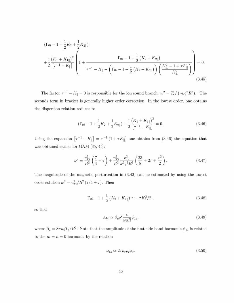
(Γ0i − 1 +1

2K2 +

1

2K2)

+1

2

K1 +K1

2τ−1 −K

1 +Γ0i − 1 +

1

2

K2 +K2

τ−1 −K −Γ0i − 1 +

1

2

K2 +K2

K2⊥ − 1 + τK

K2⊥

= 0.

(3.45)

The factor τ−1−K = 0 is responsible for the ion sound branch: ω2 = Te/miq

2R2. The

seconds term in bracket is generally higher order correction. In the lowest order, one obtains

the dispersion relation reduces to

(Γ0i − 1 +1

2K2 +

1

2K2) +

1

2

K1 +K1

2τ−1 −K

= 0. (3.46)

Using the expansionτ−1 −K

= τ−1

1 + τK

one obtains from (3.46) the equation that

was obtained earlier for GAM [35, 45]:

ω2 =v2TiR2

7

4+ τ

+

v2TiR2

v2Tiω2q2R2

23

8+ 2τ +

τ2

2

. (3.47)

The magnitude of the magnetic perturbation in (3.42) can be estimated by using the lowest

order solution ω2 = v2Ti/R2 (7/4 + τ). Then

Γ0i − 1 +1

2

K2 +K2

≃ −τK2

1/2 , (3.48)

so that

A1c ≃ βeq2 c

ωqRφ1s, (3.49)

where βe = 8πn0Te/B2. Note that the amplitude of the first side-band harmonic φ1s is related

to the m = n = 0 harmonic by the relation

φ1s ≃ 2τkrρiφ0. (3.50)

46

Plasma parameters scalings from the order of magnitude estimates (3.49) and (3.50) can be

used to identify the signatures of magnetic fluctuations in experiments.

The effects of magnetic component in Eq. (3.45) is controlled by the amplitude of the radial

mode width parameter [20] K2⊥. The electrostatic regime corresponds to the case K2

⊥ ≫ 1. In

this limit one has from Eq. (3.45)

(Γ0i − 1 +1

2K2 +

1

2K2) +

1

2

K1 +K1

2

τ−1 −K −Γ0i − 1 +

1

2

K2 +K2

= 0.

(3.51)

One can see that this limit can be obtained by setting the magnetic vector potential A1c = 0

in Eqs. (3.29-3.36). In the electromagnetic limit, K2⊥ ≪ 1, one has from Eq. (3.45)

(Γ0i − 1 +1

2K2 +

1

2K2)

+1

2

K1 +K1

2τ−1 −K

1 +

Γ0i − 1 +1

2

K2 +K2

τ−1 −K −Γ0i − 1 +

1

2

K2 +K2

/K2

⊥

= 0,

(3.52)

or

(Γ0i − 1 +1

2K2 +

1

2K2) +

1

2

K1 +K1

2

τ−1

1− K2

1τ2

2 (1 + βeq2)

= 0.

(3.53)

General structure of the roots of Eq. (3.45) is shown in Fig. (3.1) for different values of plasma

pressure along with the lowest order standard dispersion relation of GAMs

ω2 =

v2tiR2

7

4+ τ

and ion sound mode

ω2 =

v2tiτ

2q2R2

. The upper roots above the GAMs correspond to the de-

nominator of the dispersive part in expression (3.45) and are related to the Alfvén sideband

continuum ω = vA/qR branches. The lower frequency ion sound modes (below the GAM

frequency) have also been found earlier in kinetic analysis [74, 19]. The standard and lower

47

frequency ion sound modes and higher frequency modes (above GAM) will not be considered

here. So only the GAMs root is shown in Figs.(3.2-3.8). Figs.(3.2, 3.3) depict the normalized

frequencyωR

vtias function of krρi to highlight the dispersion effect on GAMs. Note that the

mode dispersion due to magnetic effect is negative. In Figs.(3.4-3.6) , we show the effect of

plasma pressure βe on GAMs for various values of plasma parameters and value of krρi. It

follows that finite plasma pressure reduces the mode frequency as shown in Figs.(3.4-3.6). The

role of the magnetic corrections on the mode dispersion is shown in Figs. (3.7) and (3.8). Here

we show the simplified leading order dispersion relation for GAMs from Eq. (3.47) in compar-

ison with the solution from full Eq.(3.45) as a function of temperature ratio τ and the safety

factor q respectively. Figs. (3.7) and (3.8) show that the mode frequency decreases with an

increase of krρi in consistence with negative dispersion due to magnetic effects.

Figure 3-1: Multiple roots of the dispersion relation (3.45) i.e., Normalized frequencyωR

vtivsas functions of krρi at different values of plasma pressure: βe =0.05 — solid line, βe = 0.07—dotted line, βe = 0.1 — dashed line, βe = 0.2 — dot-dashed line; q = 1.8 and τ = 1.6.

48

Figure 3-2: Normalized FrequencyωR

vtivs krρi for GAM branch at fixed q = 1.8 and βe = 0.2

for different values of the temperature ratio: τ = 1.6 — solid line, 1.7 — dotted line, 1.8 — dashedline, 1.9 — dot-dashed line.

Figure 3-3: Normalized frequencyωR

vtivs krρi for GAM branch at fixed τ = 1.3 and βe = 0.1

for different values of safety factor: q = 1.8 — solid line, 2.5 — dotted line, 3.5 — dashed line, 4.5— dot-dashed line.

49

Figure 3-4: Normalized frequencyωR

vtivs βe for GAM branch at fixed q = 2.5 and τ = 1.3 for

different values of normalized radial wave number: krρi = 0.1 — solid line, 0.2 — dotted line, 0.3— dashed line, 0.4 — dot-dashed line.

Figure 3-5: Normalized frequencyωR

vtivs βe for GAM branch at τ = 1.8 and krρi = 0.4 with

variation in safety factor: q = 2.0 — solid line, 2.5 — dotted line, 3.0 — dashed line, 3.5 —dot-dashed line.

50

Figure 3-6: Normalized frequencyωR

vtivs βe for GAM branch at fixed value of q = 2.5 and

krρi = 0.3 for different values of temperature ratio: τ = 1.0 — solid line, 1.3 — dotted line, 1.6 —dashed line, 1.9 — dot-dashed line.

Figure 3-7: Normalized frequencyωR

vtivs τ for GAM branch at fixed q = 3.0 as a function of

τ : a) βe = 0.1, Eq.(3.47) — solid line, krρi = 0.05 — double dotted, krρi = 0.1 — dotted line,krρi = 0.2 — dashed line, krρi = 0.4 — dot-dashed line; b) krρi = 0.1, Eq. (3.47) — solid line,βe = 0.1 — double dotted, βe = 0.2 — dotted line, βe = 0.3 — dashed line, βe = 0.4 — dot-dashedline.

51

Figure 3-8: Normalized frequencyωR

vtivs q for GAM branch at fixed τ = 1.6 as a function

of q, a) βe = 0.03, Eq. (3.47) — solid line, krρi = 0.2 — double dotted, krρi = 0.3 — dottedline, krρi = 0.4 — dashed line, krρi = 0.5 — dot-dashed line; b) krρi = 0.1, Eq. (3.47) — solidline, βe = 0.05 — double dotted, βe = 0.1 — dotted line, βe = 0.2 — dashed line, βe = 0.4 —dot-dashed line.

52

Chapter 4

Stability Analysis of

Self-Gravitational Electrostatic Drift

waves for a Streaming Non-Uniform

Quantum Dusty Magnetoplasma

Using the quantum hydrodynamical model of plasmas, the stability analysis of self-gravitational

electrostatic drift waves for a streaming non-uniform quantum dusty magnetoplasma is pre-

sented. For two different frequency domains i.e., Ω0d << ω < Ω0i (unmagnetized dust)

and ω << Ω0d < Ω0i (magnetized dust), we simplify the general dispersion relation for self-

gravitational electrostatic drift waves which incorporates the effects of density inhomogeneity

∇n0α, streaming velocity v0α due to magnetic field inhomogeneity ∇B0, Bohm potential and

the Fermi degenerate pressure. For both frequency domains, the effect of density inhomogene-

ity gives rise to real oscillations while the ions streaming velocity v0i as well as the effective

electron quantum velocity v′Fe make these oscillations propagate perpendicular to the ambient

magnetic field. This oscillatory behavior of self-gravitational drift waves increases with increase

in inhomogeneities and quantum effects while it decreases with increase in the gravitational po-

tential. However only for the unmagnetized case, the drift waves may become unstable under

appropriate conditions giving rise to Jeans instability. The modified threshold condition is also

53

determined for instability by using the intersection method for solving the cubic equation. We

note that the inhomogeneity in magnetic field (equilibrium density) through streaming veloc-

ity (diamagnetic drift velocity) suppress the Jeans instability depending upon the characteristic

scale length of these inhomogeneities. On the other hand, the dust-lower-hybrid wave and the

quantum mechanical effects of electrons tend to reduce the growth rate as expected. A number

of special cases are also discussed.

4.1 Introduction

The problem of gravitational collapse of astrophysical nebulae for the formation of stars and

galaxies has been a great challenge in astrophysics and cosmology. James Jeans [79] first showed

how a neutral fluid in a nebula containing micron-sized dust grains may become unstable due to

its own self-gravity. This is the main mechanism for the large scale nebulae in the Universe to

collapse to stars, galaxies, etc. or other structures and their evolution. It is also known that the

Jeans instability is a relatively faster process, whereas the formation of heavenly objects takes

place in billions of years [80]-[85]. Obviously, there should be a number of hindering effects on

Jeans instability, which may explain the real phenomena behind the gravitational collapse.

It is believed that due to the presence of all-pervading ultra-violet photons, plasma currents

or for some heavenly occurrences, the micron-sized dust grains of the collapsing systems can

acquire electric charges and thus a self-gravitating dusty plasma under extreme conditions may

be formed [86]-[88]. These plasmas may contain static and inhomogeneous ambient magnetic

field, nonuniform densities or even quantum effects under extreme conditions.

In recent years, there has been a growing interest in quantum plasmas because of their

importance in microelectronics and electronic devices with nano-electronic components [89, 90],

dense astrophysical systems [91]-[93], and in laser-produced plasmas [94]-[97]. When a plasma

is cooled to an extremely low temperature, the de Broglie wavelengths of the plasma particles

could be comparable to the scale lengths, such as Debye length or Larmor radius, etc. in the

system. In such plasmas, the ultracold dense plasma would behave as a Fermi gas and the

quantum mechanical effects might play a vital role in the behavior of the charge carriers of

these plasmas under the extreme conditions.

54

Extensive studies have been done over the years by taking into account a wide variety of

effects so as to study Jeans instability. Shukla and Stenflo [98] examined the influence and

the range of validity of quantum effects on Jeans instabilities of homogeneous and unmagne-

tized self-gravitating astrophysical quantum dusty plasma systems where the electromagnetic

and gravitational forces on plasma charge carriers become comparable. Ren et al.[107, 108]

investigated the Jeans instability in a dense quantum plasma in the presence of two dimen-

sional magnetic fields and the resistive effects with or without Hall current effects. Recently,

Prajapati and Chhajlani [109] discussed the contributions of Hall current and viscosity of the

medium to Jeans instability and its importance to astrophysical plasmas. The inhomogeneous

ambient magnetic field, the nonuniform plasma density, and the quantum effect might play an

important role in reducing the growth rate of the Jeans instability of the real physical plasmas.

In an earlier paper [28], we also examined Jeans instability in a homogeneous dusty plasma

in the presence of an ambient magnetic field with quantum effect arising through the Bohm

potential only.

In this chapter, we present a detailed investigation showing how the inhomogeneous ambient

magnetic field, the nonuniform density, and quantum effects influence the Jeans instability in a

self-gravitating quantum dusty magnetoplasma. We also use the intersection method developed

by Omar Khayyam [99] to solve the cubic equation and obtain minimum threshold condition

for Jeans instability.

4.2 Dielectric Response Function

We consider an infinitely extended inhomogeneous high density dusty magnetoplasma con-

taining electrons, ions and charged dust grains in the presence of an inhomogeneous ambient

magnetic field B0. We choose the Cartesian coordinate system in such a way that B0(x) is in

the z-direction with the inhomogeneity along x-direction and the wave propagation vector k is

in yz-plane. In order to satisfy the equilibrium conditions, given in Appendix A, we assume

that the streaming velocity v0α is along y-axis and the density inhomogeneity along x-axis.

Further, the charge quasi-neutrality condition is n0e(x) = n0i(x) +Zd n0d(x) where n0α(x) is

the equilibrium inhomogeneous number density of α-species (α = e, i, d), Zd is the dust charge

55

state. The density inhomogeneity produces diamagnetic drifts, and the magnetic field inhomo-

geneity causes uniform streaming of ions and electrons (not for heavy dust particles i.e., v0d

= 0) with v0e,i = −c ∂B0(x)/∂x

4πqdnody. Such plasmas may exist in the interiors and environments

of astrophysical compact objects e.g., white dwarfs and neutron stars/magnetars, supernovae,

etc [111]. The governing linearized equations for electrostatic wave propagation in the quantum

hydrodynamic (QHD) model [101]-[105] for the electrons, ions and charged dust grains in the

presence of the inhomogeneous ambient magnetic field B0(x) are

mαn0α

∂v1α∂t

+ (v0α.∇)v1α

= n0αqα

E1 +

1

cvα ×B0

−KTFα∇n1α

−mαn0α∇ψ1 +

4mα∇∇2n1α

, (4.1)

and∂n1α∂t

+ v0α.∇n1α + v1α.∇n0α + n0α∇ · v1α = 0. (4.2)

Poisson’s equations for the perturbed electrostatic potential φ1 and gravitational potential

ψ1 are

∇2φ1 = −4π

qαn1α, (4.3)

and

∇2ψ1 = 4πGmαn1α, (4.4)

where subscript 0 indicates equilibrium quantities while 1 is used for the perturbed quanti-

ties, summation over α is for the three species i.e., (α = e, i, d), is Planck’s constant divided

by 2π and qα,mα, c and G are the charge, mass, the velocity of light in vacuum and gravi-

tational constant respectively. Here, we may take into account the quantum effects of all the

species when they are considered extremely cold. In Eq. (4.1), we assume that the plasma

particles in a zero-temperature Fermi gas satisfying the pressure pFα = mαv2Fαn1α/3n20α where

vFα = (2kBTFj/mj)1

2 is the Fermi speed; kB and TFj are the Boltzmann constant and Fermi

temperature respectively.

56

By assuming that perturbations have sinusoidal character i.e.,

(E1, B1,n1α,v1α) ≈ e− i ω t+ i k·r , (4.5)

we may rewrite the equations (4.1-4.4) as

v1α =qαk φ1ω∗mα

+i

ω∗v1α ×Ω0α +

kv′2Fαω∗

n1αn0α

+k

ω∗ψ1, (4.6)

n1αn0α

=

k · v1αω∗

+

ivx1αLαω∗

, (4.7)

k2φ1 = 4π

q0αn1α, (4.8)

k2ψ1 = −4πGmαn1α. (4.9)

Here, ω and k are the angular frequency and wavenumber vector, respectively. We have also

defined

v′2Fα = v2Fα +2k2

4m2α

, Ω0α =qαB0mαc

z and ω∗ = ω − kyv0α .

Using Eqs. (4.6-4.9) and after some straightforward calculations, we obtain the general dielectric

susceptibility for a dusty magnetoplasma with magnetic field and density inhomogeneities as

χα = −ω2pα

'k2z

(ω∗)2+

k2y

(ω∗)2 −Ω20α

1− Ω0α

ω∗kyLα

(

k2 −'

k2z(ω∗)2

+k2y

(ω∗)2 −Ω20α

1− Ω0α

ω∗kyLα

(k2v′2Fα − ω2Jα

, (4.10)

where

ω2pα =4πn0αq

2α

mα, ω2Jα = 4πGmαn0α and Lα = − n0α

∂n0α/∂x.

Using the above equation (4.10), the electrostatic dielectric response function is given by

57

ǫ (ω, k) = 1 +

α

χα = 1−

α

ω2pα

'k2z

(ω∗)2+

k2y

(ω∗)2 −Ω20α

1− Ω0α

ω∗kyLα

(

k2 −'

k2z(ω∗)2

+k2y

(ω∗)2 −Ω20α

1− Ω0α

ω∗kyLα

(k2v′2Fα − ω2Jα

.

(4.11)

Eq. (4.11) is the electrostatic dielectric response function which incorporates the effects of

inhomogeneities, quantum effects through both the Fermi potential and the Bohm potential and

the effect of gravitational potential. On ignoring the inhomogeneities, this function immediately

reduces to the previously derived response function [28].

In the following, we shall derive the dispersion relation for the self-gravitational electrostatic

drift waves including the quantum effects for the electron dynamics, density inhomogeneity for

electrons and ions and the gravitational effects for dust grains. The quantum effects on ions

and dust grains are neglected due to their heavier masses. Also, being insignificantly small, we

can neglect the gravitational effects on electrons and ions. However, for dust grain, the self-

gravitational effect is taken into account. Thus for such plasmas satisfying the above conditions

and assuming that the wave frequency and Doppler shifted frequency is much less than the gyro

frequency of electron i.e., ω, ω∗ << |Ω0e| and the phase velocity of the wave is less than the

effective electron (quantum) velocity but greater than the ion one i.e.,v′Fi << ω/kz << v′Fe ,

we can write the dispersion relation of electrostatic waves i.e., ǫ(ω, k) = 0 by simplifying Eq.

(4.11) as

1 +ω2pe

k2v′2Fe−

ω2pik2

k2z

(ω∗)2+

k2y

(ω∗)2 −Ω20i

1− Ω0i

kyω∗Li

−

ω2pd

k2zω2

+k2y

ω2 −Ω20d

k2 +

k2zω2

+k2y

ω2 −Ω20d

ω2jd

= 0.

(4.12)

The condition for the phase velocity (i.e., v′Fi << ω/kz << v′Fe) defines that electrons which

run along magnetic lines will reach thermal equilibrium condition quickly whereas ions can not

reach thermal equilibrium and should be described by the drift equation.

In the following, we will discuss two frequency domains i.e., Ω0d << ω < Ω0i for unmagne-

tized dust and ω << Ω0d < Ω0i for magnetized dust grains.

58

4.2.1 For Unmagnetized Dust Grains

For this case, we shall assume the intermediate frequency domain i.e., the wave frequency lies

between the gyro frequencies of dust and ions (Ω0d << ω < Ω0i) . Thus the dispersion relation

reduces to

1 +ω2pe

k2v′2Fe−

ω2pik2

k2z

(ω∗)2−

k2yΩ20i

1− Ω0i

kyω∗Li

−

ω2pdω2 + ω2jd

= 0. (4.13)

If we assume that the propagation is predominantly perpendicular i.e., k2z << k2y, the above

equation takes a simpler form

1 +ω2pe

k2yv′2Fe

+ fi −ω′iω∗−

ω2pdω2 + ω2Jd

= 0, (4.14)

where

ω′i =ω2pi

Ω0iLikyand fi =

ω2piΩ20i

.

From Eq. (4.14), we notice that the drift wave may become unstable due to the presence

of dust particles satisfying the certain threshold conditions for both the inhomogeneous plasma

(i.e., ω′i = 0) and the homogeneous (i.e., ω′i = 0). In the absence of dust particles, we only

obtain the real oscillations in the former case while in the latter no wave would exist. We

also note that for the plasma system satisfying above assumptions (see Appendix F. and Eq.

(4.14)), the effect of streaming will appear only if the inhomogeneities in both the ambient

magnetic and the equilibrium density are present.

We may rewrite the above Eq. (4.14) as

0 = ω3 −kyv0 + ω′i/fiF

ω2 + ω

ω2Jd − ω2dlh/F

−)

kyv0 + ω′i/fiF

ω2Jd − ω2dlh/F+ω2dlh/F

ω′i/fiF

*, (4.15)

where

F = 1 +1

fi+

ω2pefik2yv

′2Fe

, ωdlh =ωpdΩ0iωpi

.

The above equation becomes cubic in ω due to inhomogeneities and gives three roots. We

observe that one root remains always real where as the other two roots can become complex

59

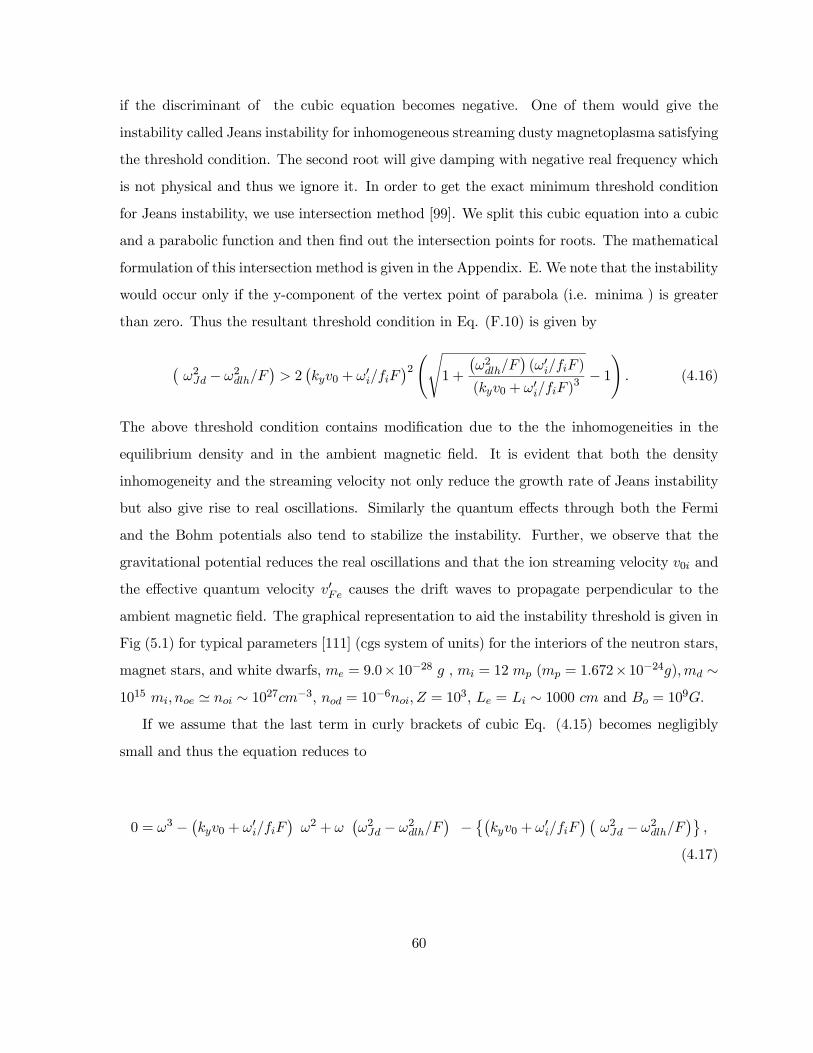
if the discriminant of the cubic equation becomes negative. One of them would give the

instability called Jeans instability for inhomogeneous streaming dusty magnetoplasma satisfying

the threshold condition. The second root will give damping with negative real frequency which

is not physical and thus we ignore it. In order to get the exact minimum threshold condition

for Jeans instability, we use intersection method [99]. We split this cubic equation into a cubic

and a parabolic function and then find out the intersection points for roots. The mathematical

formulation of this intersection method is given in the Appendix. E. We note that the instability

would occur only if the y-component of the vertex point of parabola (i.e. minima ) is greater

than zero. Thus the resultant threshold condition in Eq. (F.10) is given by

ω2Jd − ω2dlh/F

> 2

kyv0 + ω′i/fiF

2

1 +

ω2dlh/F

(ω′i/fiF )

(kyv0 + ω′i/fiF )3− 1

. (4.16)

The above threshold condition contains modification due to the the inhomogeneities in the

equilibrium density and in the ambient magnetic field. It is evident that both the density

inhomogeneity and the streaming velocity not only reduce the growth rate of Jeans instability

but also give rise to real oscillations. Similarly the quantum effects through both the Fermi

and the Bohm potentials also tend to stabilize the instability. Further, we observe that the

gravitational potential reduces the real oscillations and that the ion streaming velocity v0i and

the effective quantum velocity v′Fe causes the drift waves to propagate perpendicular to the

ambient magnetic field. The graphical representation to aid the instability threshold is given in

Fig (5.1) for typical parameters [111] (cgs system of units) for the interiors of the neutron stars,

magnet stars, and white dwarfs, me = 9.0×10−28 g , mi = 12 mp (mp = 1.672×10−24g),md ∼1015 mi, noe ≃ noi ∼ 1027cm−3, nod = 10−6noi, Z = 103, Le = Li ∼ 1000 cm and Bo = 109G.

If we assume that the last term in curly brackets of cubic Eq. (4.15) becomes negligibly

small and thus the equation reduces to

0 = ω3 −kyv0 + ω′i/fiF

ω2 + ω

ω2Jd − ω2dlh/F

−)

kyv0 + ω′i/fiF

ω2Jd − ω2dlh/F*

,

(4.17)

60

Figure 4-1: This figure represents the graph of f(ω) vs ω for Eq. (4.15). Solid curve is forf(ω) = ω3 and dotted curves are for f(ω) = B ω2−ω C + G for set of parameters given afterEq. (4.16) with variation of streaming velocity as (i) dotted for v0 = 10−7c, (ii) small dashedfor v0 = 3× 10−7c (iii) large dashed for v0 = 5× 10−7c.

61

which may be factorized as

)ω2 +

ω2Jd − ω2dlh/F

*)ω −

kyv0 + ω′i/fiF

*= 0. (4.18)

The first root gives the growth rate of Jeans instability as

γ =ω2Jd − ω2dlh/F

12 , (4.19)

with the threshold condition

ω2Jd − ω2dlh/F > 0,

or ωpeωpd

ωdlh

ω2dlhω2Jd

−

1 +Ω20iω2pi

12

≥ kyv′Fe. (4.20)

The second root gives real oscillations propagating with the streaming and the Fermi velocities

as

ωr = kyv0 + ω′i/fiF. (4.21)

Eqs. (4.19, 4.21) show that due to the presence of inhomogeneities, the real propagating

oscillatory behavior is also observed with the Jeans instability. We observe that the dust-lower-

hybrid wave and the quantum mechanical effects of electrons tend to reduce the growth rate.

We also note that real frequency of self-gravitational drift waves increases with the increase in

both the inhomogeneities and the quantum effects through the Fermi and the Bohm potentials.

The expression for the growth rate in Eq. (4.19) is different from the previously derived

result [28] as it contains the contribution of quantum effects of electrons instead of dust grains.

Thus as a result, we obtain a new threshold condition on wavenumber for the instability to

occur. For the chosen parameters, the general threshold condition given in Eq. (4.16) also

immediately reduces to the above condition given in Eq. (4.20) because the second term in the

square root becomes negligibly small.

Eq. (4.15) is plotted in Fig.(4.1) for the above set of parameters. We observe that

62

the real frequency increases with the increase of streaming velocity. We also note that for

these parameter the values of the real frequency fulfill the condition of Ω0d << ω < Ω0i.

For homogeneous plasma for which ω′i → 0, Eq. (4.14) becomes

ω2 = −ω2Jd + ω2dlh/F , (4.22)

giving purely growing Jeans instability as

γ =ω2Jd − ω2dlh/F

12 . (4.23)

If the gravitational potential is absent, Eq. (4.14)

1 +ω2pe

k2yv′2Fe

+ fi −ω′iω∗−

ω2pdω2

= 0,

or

1− (ω′i / fiF )

ω∗− ω2dlh /F

ω2= 0. (4.24)

This is the same dispersion relation as derived by Salimullah et al. [100] and by letting

ω = kyv0i + δ where δ << kyv0i, the above equation becomes

1− (ω′i / fiF )

δ− ω2dlh /F

k2yv20i

1− 2δ

kyv0i

= 0.

The growth rate of drift wave is given by (ω = ωr + iγ)

γ =

|ω∗i | k3yv30√

2ωpd

+,,-1−ω2pd

8 |ω∗i | kyv0

k2yv

20

ω2pd/F′− 1

2, (4.25)

where

F ′ = 1 +ω2pek2v′2te

+ fi/

This growth rate of drift wave is more general with the threshold condition

63

|ω∗i | >ωpd

2√

2kyv0

k2yv

20

ω2pd/F′− 1

, (4.26)

If we assume kyv0i ∼ ωpd /√F ′, it immediately reduces to the result of Salimullah et al.

[100] i.e.,

γ =ωpi (kyv0i)

3

2

√2ωpd

kyΩ0i |Li|

. (4.27)

4.2.2 For Magnetized Dust Grains

If the dust is also magnetized, the dispersion relation Eq.(4.12) takes the form

1 +ω2pe

k2v′2Fe−

ω2pik2

k2z

(ω∗)2−

k2yΩ20i

1− Ω0i

kyω∗Li

−

ω2pd

k2zω2−

k2yΩ20d

k2 +

k2zω2−

k2yΩ20d

ω2jd

= 0. (4.28)

For perpendicular propagation, (i.e., kz = 0) , the above equation reduces to

1− (ω′i / fiF )

ω∗+

ω2dlh /F

Ω20d − ω2jd

= 0, (4.29)

or

ω = kyvy0i +

(ω′i / fiF )1 +

ω2dlh /F

Ω20d − ω2jd

. (4.30)

From the above equation it is evident that for the magnetized dust grains, we only obtain

stable wave and that the frequency reduce with the increase in the gravitational potential.

64

Chapter 5

Summary of Results and Discussion

In Chapter 2, the drift kinetic theory is used to derive the full kinetic dispersion relation

for the Geodesic acoustic modes (GAMs) including diamagnetic effects due to inhomogeneous

plasma density and temperature. The fluid model, including the effects of ion parallel viscosity

(pressure anisotropy) is used to recover exactly the adiabatic index obtained in kinetic theory.

GAM results from the balance between the ion polarization current (Eq. (2.45)) and the

geodesic current (Eq. (2.46)), which is produced by the M = ±1 side-bands of the perturbed

pressure (together with parallel viscosity [27]). The pressure side-bands are in turn created by

the flow due to M = 0 mode of the electrostatic potentia l[16]. As pointed out by [35], GAMs

are degenerated in the absence of diamagnetic effects in the q >> 1 approximation. Drift effects

directly affect the diamagnetic current, (Eq. (2.43)), breaking the symmetry of the dispersion

relations (Eqs.(2.47,2.48)) removing the degeneracy of the zero frequency zonal flow mode.

The instability occurs for high temperature gradients ηi > 3/4. The grow rate of this

instability, which is associated with the zonal flow branch, as well as the modification of the

GAM frequency are typically small for density/temperature gradients length scale of the order of

the minor radius, i.e., γ ∼ (ρiR0/rLn)ωgam. However, in the region of large density/temperature

gradients, the drift corrections may become of the similar order as the GAM frequency.

To our knowledge this instability of the ZF/GAM type mode has not been studied before,

though we have shown that our final dispersion relation is a special case of a more general

fishbone-like dispersion relation obtained by Zonca et al., [50]. The fluid model presented in

65

this section provides a transparent treatment of the diamagnetic drift corrections and thus a

shorter path to the understanding of the physical mechanism. The fluid treatment is also more

easily generalized to the nonlinear case. One has to note that technically, the fluid treatment

requires the condition ω > vti/qR0, therefore our results are valid either in high q regimes, or

in case of large plasma gradients, so that ω∗ > vti/qR0. In stable case, ηi < 3/4, the dispersion

relation (2.48), produces two GAM type modes, which, in the region of high density gradient,

can have comparable frequencies. It is of interest to note that in experiments, there are two

modes with close frequencies observed [51],[52]. One can conjecture that this mode splitting is

due to plasma gradients effects.

Previously, the effect of equilibrium (poloidal and toroidal) rotation on GAM were inves-

tigated within the framework of one fluid MHD theory in [53],[54]. It was found that the

equilibrium plasma rotation induces not only the sin θ, but also cos θ component of the per-

turbed density (and pressure); θ is the poloidal angle in toroidal configuration with equilibrium

magnetic field B = B0(1 − ǫ cos θ), ǫ = r/R0, where r is the minor and R0 are major radii.

In this respect, density gradients have similar effect as equilibrium rotation [53], [54], caus-

ing the perturbed density to depend also on cos θ (Eq. (2.34)) and φc = 0 (Eq. (2.37)), i.e.,

ni = O(k2rρ2i ) + O(krρi) sin θ +O(krρi) cos θ and φ = φ0 + φs sin θ + φc cos θ. Higher order

of dispersive terms, O(k4rρ4i ), which are important to understand the radial structure of GAM,

although not included in this paper, can be obtained by accounting for φ±2.

Similar dispersion relation for electromagnetic modes including dispersive terms were derived

in [38], [39] (see also [18], [35]). It is expected that, generally, φk ∼ (krρi)kφ0 (Eq. (2.37)), ni0 ∼

k2rρ2i

eφ0/Ti

, ni±1 ∼ krρi

eφ0/Ti

(Eq. (2.34)) [31], and, hence, as confirmed previously[16]

the main quantities involving in the basic GAM study are φ0 and ρs sin θ (mass density).

In Chapter 3, we have used the drift kinetic equation to derive the general dispersion

relation for GAMs which incorporates the effect of magnetic perturbation. We have derived

general dispersion relation for arbitrary values of se = ωqR/vTe and si = ωqR/vTi. The

latter includes the dispersive as well as damping effects. The simplified plasma response in

the electron adiabatic (se < 1) and fluid ion (si > 1) regimes were also obtained showing the

magnetic effect explicitly. The main result is that the GAM have finite magnetic component

in the first side-band contrary to the result in Refs. [69, 73]. It is worth noting that the

66

amplitude of the magnetic vector potential does not contain the additional small parameter

krρi as suggested in Refs. [69, 73], but is controlled by the value of the βeq2 parameter. For

βeq2 ≃ 1, the amplitude of the magnetic vector potential is of the same order as the main

GAM sideband φ1s [see Eq. ((3.49))]. We note that βeq2 parameter can be large as e.g., in

NSTX tokamak[55]. The dependence of GAM frequency on βe is shown in Figs. (3.4)-(3.6).

It was recently noted that the value of the βeq2 parameter also responsible for the coupling of

m = n = 0 mode to the m = 2 harmonics [75]. The effect investigated in our paper is different

since it is concerned with the magnetic component of the m = 1 harmonics. Essentially, it is

a two-fluid effect since we assume different regimes for the electron and ion responses: se < 1

and si > 1. It is interesting that in the lowest order, the GAM dispersion relation is largely

insensitive whether the m = 1 side-band is electrostatic or electromagnetic. It may be noted

that the transition to the electromagnetic regime requires the large radial mode width, K2⊥ < 1;

K2⊥ ≃ τk2rc

2/q2ω2pi

≃ τk2rρ

2i /βiq

2. The theoretical dependencies of the amplitude of the

magnetic and side band harmonics shown in Eqs. (3.49), (3.50), can be used for experimental

identification of these effects.

The effects of plasma pressure βe, the safety factor q and the temperature ratio τ on GAM

dispersion have been analyzed here. We note that the dispersion is negative for GAMs in

some regions and this dispersion shifts to lower (higher) frequency with the increase in the

plasma pressure βe and safety factor q (temperature ratio τ). The full study of the dispersion

effects requires the inclusion of the second harmonics. We outline full route to the calculations

of the second harmonics effects and the differences with previous work in Appendix E. The

investigation of the dispersive effects (up to the second order) as well as the mode damping

[45] in full electromagnetic model is left for future work. It is expected that the amplitude

and the phase relations for plasma parameters fluctuations may be important for experimental

identification of GAM magnetic m = 1 component.

In Chapter 4, The stability analysis of self-gravitational electrostatic drift waves for a

streaming non-uniform quantum dusty magnetoplasma by using the quantum hydrodynamic

model of plasmas is presented. Incorporating the effects of density inhomogeneity∇n0α, stream-

ing velocity v0α due to magnetic field inhomogeneity ∇B0, Bohm potential and the Fermi

degenerate pressure, we first derive the general dispersion relation for self-gravitational electro-

67

static drift waves and then simplify it for two different frequency domains i.e., Ωd << ω < Ωi

(unmagnetized dust) and ω << Ωd < Ωi (magnetized dust).

For both frequency domains, the effects of density inhomogeneity give rise to real oscilla-

tions and the ion streaming velocity v0i and the effective quantum velocity provide the source

to propagate these oscillations perpendicular to the ambient magnetic field. This oscillatory

behavior of self-gravitational electrostatic waves increases with increase in inhomogeneities and

decreases with increase in quantum effects through both the Bohm potential and fermi potential

and in gravitational potential.

We also note that for the magnetized case, the available free energy through density inhomo-

geneity and the streaming velocity is not sufficient to make the drift waves unstable. However

only for the unmagnetized case, the electrostatic drift waves may become unstable under appro-

priate conditions. These unstable self-gravitational drift waves give rise to Jeans instability and

by using the intersection method for solving cubic equation, we also determine the threshold

condition for Jeans instability. We also note that the inhomogeneity in the ambient magnetic

field ( equilibrium density) through streaming velocity (diamagnetic drift velocity) suppress the

Jeans instability depending upon the characteristic scale length of these inhomogeneities. On

the other hand, the dust-lower-hybrid wave and the quantum mechanical effects of electrons

tend to reduce the growth rate.

For the unmagnetized case, we further simplify the dispersion relation for growth rate in

some limiting cases. e.g., in the absence of gravitational potential, we obtain a new dispersion

relation for the growth rate of drift wave instability in non-uniform quantum dusty magneto-

plasma which incorporates the quantum effects through electrons. We also retrieve the growth

rates of Jeans instability in a homogeneous dusty magnetoplasma.

Our results in this paper may be useful for the study of Jeans instability and the possible

drift waves for the nonuniform streaming dusty quantum plasmas which may occur e.g., in

dense astrophysical systems i.e., the interiors of white dwarfs and neutron stars [91, 92, 93],

laser-produced plasmas [94, 95, 96, 97] and in the laboratory plasmas[89, 90].

68

Chapter 6

Appendixes

6.1 Appendix A

The required integrals for the derivation of general dispersion relation are

Γ0α =1

n0

J20 (zα)FMαd

3v (A.1)

Γ0α =

1

n0

J20 (zα)

v2

v2tαFMαd

3v (A.2)

I00α =1

n0

ω2

WJ20 (k⊥v⊥/ωci) FMαd

3v (A.3)

I01α =1

n0

ω2

WJ20 (k⊥v⊥/ωci)

v2

v2tαFMαd

3v (A.4)

I02α =1

n0

ω2

WJ20 (k⊥v⊥/ωci)

v4

v4tαFMαd

3v (A.5)

I10α =1

n0

v2⊥/2 + v2

v2tα

ω2

WJ20 (k⊥v⊥/ωci) FMαd

3v (A.6)

I11α =1

n0

v2⊥/2 + v2

v2tα

v2

v2tα

ω2

WJ20 (k⊥v⊥/ωci) FMα d3v (A.7)

I20α =1

n0

v2⊥/2 + v2

2

v4tα

ω2

WJ20 (k⊥v⊥/ωci) F0 d3v (A.8)

I21α =1

n0

v2⊥/2 + v2

v2tα

2v2

v2tα

ω2

WJ20 (k⊥v⊥/ωci) FMαd

3v (A.9)

69

and the drift integrals are

I00∗ =1

n0

Qα

ω2

WJ20 (k⊥v⊥/ωci) FMαd

3v = I00α + ηαP00α (A.10)

P 00α =1

n0

ω2

W

v2

v2Ti− 3

2

J20 (k⊥v⊥/ωci) FMαd

3v (A.11)

I10∗α =1

n0

QαQ

v2⊥/2 + v2

v2Ti

ω2

WJ20 (k⊥v⊥/ωci) FMα d3v = I10α + ηαP

10α (A12)

P 10α =1

n0

v2⊥/2 + v2

v2Tα

v2

v2Tα− 3

2

ω2

WJ20 (k⊥v⊥/ωci) FMαd

3v (A13)

I20∗α =1

n0

Qα

v2⊥/2 + v2

2

v4Ti

ω2

WJ20 (k⊥v⊥/ωci) FMα d3v = I20α + ηαP

20α (A.14)

P 20α =1

n0

v2⊥/2 + v2

2

v4Ti

v2

v2Ti− 3

2

ω2

WJ20 (k⊥v⊥/ωci) FMα d3v (A.15)

with

Qα = 1 + ηα

v2

v2Ti− 3

2

(A.16)

70

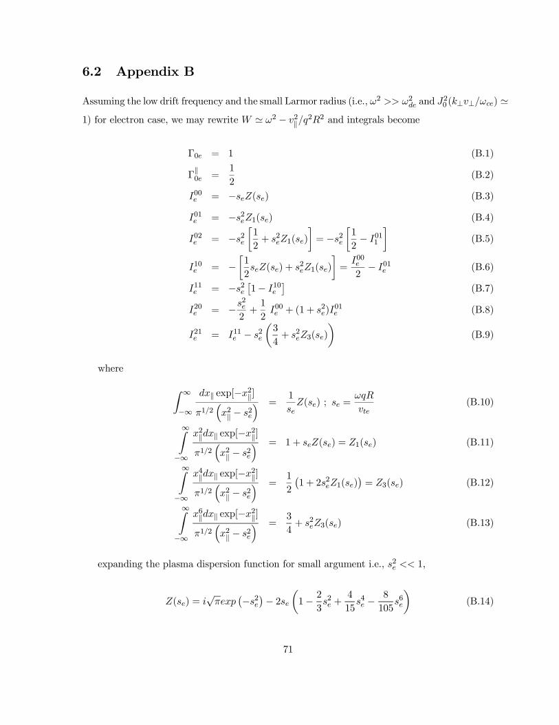
6.2 Appendix B

Assuming the low drift frequency and the small Larmor radius (i.e., ω2 >> ω2de and J20 (k⊥v⊥/ωce) ≃1) for electron case, we may rewrite W ≃ ω2 − v2/q

2R2 and integrals become

Γ0e = 1 (B.1)

Γ0e =

1

2(B.2)

I00e = −seZ(se) (B.3)

I01e = −s2eZ1(se) (B.4)

I02e = −s2e1

2+ s2eZ1(se)

= −s2e

1

2− I011

(B.5)

I10e = −1

2seZ(se) + s2eZ1(se)

=

I00e2− I01e (B.6)

I11e = −s2e1− I10e

(B.7)

I20e = −s2e2

+1

2I00e + (1 + s2e)I

01e (B.8)

I21e = I11e − s2e

3

4+ s2eZ3(se)

(B.9)

where

∞

−∞

dx exp[−x2]

π1/2x2 − s2e

=1

seZ(se) ; se =

ωqR

vte(B.10)

∞

−∞

x2dx exp[−x2]

π1/2x2 − s2e

= 1 + seZ(se) = Z1(se) (B.11)

∞

−∞

x4dx exp[−x2]

π1/2x2 − s2e

=1

2

1 + 2s2eZ1(se)

= Z3(se) (B.12)

∞

−∞

x6dx exp[−x2]

π1/2x2 − s2e

=3

4+ s2eZ3(se) (B.13)

expanding the plasma dispersion function for small argument i.e., s2e << 1,

Z(se) = i√πexp

−s2e

− 2se

1− 2

3s2e +

4

15s4e −

8

105s6e

(B.14)

71

we may reduce the integrals electron expressions. In what follows we neglect the imaginary

part

I00e = 2s2e −4

3s4e (B15)

I01e = −s2e + 2s4e (B16)

I02e = −s2e2− s4e (B17)

I10e =4

3s4e −

16

15s6e (B.18)

I11e = −s2e +4

3s6e (B.19)

I20e = −s2e2

+s4e3

(B.20)

I21e = −7

4s2e −

s4e2

(B.21)

As we consider the ηe is negligibly small, so that the result of integrals (A.10-A.15) becomes

similar to the above integrals.

6.3 Appendix C

The ion expressions are calculated with the expansion

ω2

W= 1 +

v2ω2q2R2

+ω2di2ω2

+v2ω

2di

q2R2ω4(C.1)

and

J20 (zi) = 1− 1

2

k2rv2⊥

Ω2i(C2)

72

Γ0i =1

n0

J20 (k⊥v⊥/ωci)FMid

3v = 1− 1

2k2rρ

2i (C.3)

Γ0i =

1

n0

J20 (k⊥v⊥/ωci)

v2

v2tiFMid

3v =1

2− k2rρ

2i

4(C.4)

I00i =1

n0

ω2

WJ20 (k⊥v⊥/ωci) FMid

3v

= 1− 1

2k2rρ

2i +

1

2s2i+

7

8

ω2diω2

+23

8

ω2dis2iω

2(C.5)

I01i =1

n0

ω2

WJ20 (k⊥v⊥/ωci)

v2

v2tiFMid

3v

=1

2− k2rρ

2i

4+

3

4s2i+

23

16

ω2diω2

+141

16

ω2dis2iω

2(C.6)

I02i =1

n0

ω2

WJ20 (k⊥v⊥/ωci)

v4

v4tiFMid

3v

=3

4− 3

8k2rρ

2i +

15

8s2i+

141

32

ω2diω2

+1185

32

ω2dis2iω

2(C.7)

I10i =1

n0

v2⊥/2 + v2

v2ti

ω2

WJ20 (k⊥v⊥/ωci) FMid

3v

= 1− 3

4k2rρ

2i +

1

s2i+

9

4

ω2diω2

+87

8

ω2dis2iω

2(C.8)

I11i =1

n0

v2⊥/2 + v2

v2ti

v2

v2ti

ω2

WJ20 (k⊥v⊥/ωci) FMi d

3v

= 1− 5

8k2rρ

2i +

9

4s2i+

87

16

ω2diω2

+171

4

ω2dis2iω

2(C.9)

I20i =1

n0

v2⊥/2 + v2

2

v4Ti

ω2

WJ20 (k⊥v⊥/ωci) FMi d

3v

=7

4− 13

8k2rρ

2i +

23

8s2i+

249

32

ω2diω2

+1641

32

ω2dis2iω

2(C.10)

I21i =1

n0

v2⊥/2 + v2

v2ti

2v2

v2ti

ω2

WJ20 (k⊥v⊥/ωci) FMid

3v

=23

8− 33

16k2rρ

2i +

141

16s2i+

1641

64

ω2diω2

+15867

64

ω2dis2iω

2(C.11)

with ρi = vti/Ωi and si = ωqR/vti.

The drift integrals for ions by using the assumptions used in the case of drift effects on

GAMs become as

73

I00∗i =1

n0

Qi

ω2

WJ20 (k⊥v⊥/ωci) FMαd

3v ≃ 1 +1

2s2i(1 + 2ηi) (C.12)

I10∗i =1

n0

Qi

v2⊥/2 + v2

v2Ti

ω2

WJ20 (k⊥v⊥/ωci) FMα d3v ≃ 1 + ηi +

1

s2i(1 + ηi) (C.13)

I20∗α =1

n0

Qα

v2⊥/2 + v2

2

v4Ti

ω2

WJ20 (k⊥v⊥/ωci) FMα d3v =

7

4+

23

8s2i+

ηis2i

(C.14)

6.4 Appendix D

Using the expansions of electrons and ions, we may simplify the coefficients as

S01 = Γ0i − 1 +1

2K2 +

1

2K2 (D.1)

S02 = 1 + 2K (D.2)

S03 = S02 (D.3)

S1 = −S01 (D.4)

S2 = K − τ−1 (D.5)

D1 = S2 (D.6)

Resultantly, we obtain

S1S2D1

− S2 +D1 = S1 (D.7)

S03S02

S2D1

− 1 = 0 (D.8)

ωdiω

S02 = K1 +K1 (D.9)

Where

K1 =ωdiω

, K2 =7

4

ω2diω2

, K =1

2s2i, K1 =

ωdiω

1

s2iand K2 =

23

8

ω2dis2iω

2

74

6.5 Appendix E

Here we describe the differences of our approach with that of the Refs. [69, 73]. Ref. [69]

employs the perturbative solution of the drift kinetic equation which corresponds to the zero

Larmor radius limit of the gyrokinetic equation (2) used in our work, zα → 0, J20 (zα) → 1. As

result, the finite Larmor radius effects, which are of the same order as magnetic drift effects

(or the Finite Orbit Width effects, in terminology of Ref. [69], k2rρ2i ≃ ω2d/ω

2 are neglected

in Ref. [69]. The second important point is neglect of the coupling to the zeroth harmonic of

the distribution function in Eqs. (1a, 1b) of Ref. [69], is described by the first terms in Eqs.

(3.5,3.7), see also Eqs. (E.8-E.10). As a result, a number of the second order terms are missing

in Ref. [69]. Namely, our expression (3.13) for f1s has the structure similar to Eq. (2b) of

Ref. [69] but with the following corrections: the factor in front of the φ1s term in Ref. [69] is

replaced in our work with

v2

v2 − (qRω)2→

v2 + ω2d/2q2R2ω2

v2 − (qRω)2 + ω2d/ (2q2R2ω2)J20 (zα). (E.1)

Similarly, the factors in all other terms in Eq. (2b) [69] should be replaced as

1

v2 − (qRω)2→ 1

v2 − (qRω)2 + ω2d/ (2q2R2ω2)J20 (zα). (E.2)

The resonant factors in Eq. (2c) for f1c [69] should also be replaced:

1

v2 − (qRω)2→ 1

v2 − (qRω)2 + ω2d/ (2q2R2ω2)J20 (zα). (E.3)

Note that there is a number of typos in Eq. (2c); after these typos are corrected, this equation

becomes similar to our Eq. (3.12) with the above noted factors replacements (Eqs. (E.1-

E.3). Therefore the terms of the k2rρ2i and ω2d/ω

2 are incompletely included in Ref. [69].

The n1s density component expression in Ref. [69] is missing theΓ0i − 1 + 1

2K2 + 1

2K2

φ1s

term (compare with our Eq. (3.35)). It is this last term which is responsible for a finite

value of the first harmonic of parallel current and magnetic field perturbation. It can be of

the same order as the retained term with K, since most generally, K ≃ k2rρ2i < 1. The

75

neglect of the coupling to f0 becomes critical for correct calculation of the second harmonics of

the ion distribution function (and density), which are of the second order with respect to φ0,

n2s,c/n0 ≃ ω2d/ω2 (eφ0/Ti). As shown in Appendix E, in this case the factor

v2 − (qRω)2

−1

has to be replaced with the function D given by Eq. (E.10) which produces additional terms

of the order of ω2d/ω2 missed in Ref. [69] .

Alternatively, the kinetic effects in GAM could be investigated via the formal solution of the

gyrokinetic equation in the form of infinite series of Bessel functions [74, 68, 45]. This approach

was used in Ref. [73] to investigate the electromagnetic and second order effects. The starting

point is the same equation (3.2) which is written as

ω + ωdα sin θ +

ivqR

∂

∂θ

gα = ωJ20 (zα) (φ−

vcA)

eαFMα

Tα. (E.4)

This equation can be formally integrated giving the solution in the form [74, 68, 45]

ga =eαFMα

Tα

∞

l=−∞

J20 (krv⊥/ωcα)∞

m,n=−∞

im−n exp (i (m− n) θ)

×ωJm

ωdαqR/v

JnωdαqR/v

ω − (n− l) v/qR(exp (ilθ)φl −

vcAl exp (ilθ)) (E.5)

This expression is a basis of the method in Ref. [73]. In this form the contribution of the

harmonics of poloidal sidebands φ±1, φ±2, .., can be represented by the product of two infinite

series, one in ωdαqR/v and the other in v/ωqR expansions. This basis, though formally correct

is not consistent with natural expansion parameters for GAM modes: k2rρ2i < 1 and ω2d/ω

2 < 1.

The basic GAM ordering follows from the balance of the radial polarization current against

the radial diamagnetic current

k2rρ2s

eφ0Te

≃ ωdω

p±1p0

. (E.6)

The pressure oscillations are determined by the finite compressibility of poloidal plasma flow

due to the inhomogeneous magnetic field

ωp±1p0

≃ ωdeφ0Te

. (E.7)

This balance determines the GAM frequency ω2 ≃ ω2d

k2rρ2s

≃ τev2Ti

R2. It is easy to see that natural

76

expansion for higher order (dispersive) corrections to GAM frequency is based on the expansion

in two parameters: k2rρ2i and ω2d/ω

2, and their products. It is important to note that the basic

GAM balance in Eqs. (E.6, E.7) naturally define that these two expansion parameters are of the

same order. The contribution of the ion sound effect is determined by the subsidiary expansion

in v/ (ωqR) parameter, while the Landau damping corresponds to the maximal ordering ω ≃v/qR. In our approach, presented in Eqs. (3.5-3.7), following Refs. [17, 78], the expansions

in ω2d/ω2 and v/ (ωqR) can be traced and explicitly written down via the expansion of the W

function in Eqs. (3.8-3.10). The expansion in k2rρ2i is multiplicative and follows from the J20 (zα)

function in Eqs. (3.8-3.10).

In the approach of Eq. (E.5), there are two infinite series involving the products of the Bessel

functions: JmωdαqR/v

JnωdαqR/v

and resonance denominator

ω − (n− l) v/qR

−1.

The latter is responsible for Landau damping resonances. It is known however that in toroidal

geometry the Landau resonance is modified by the ωd corrections [76, 77]. This is clearly seen

from the structure of the W function in our Eqs. (3.8-3.10), W = ω2 − v2/q2R2 − ω2dα/2. In

the fluid limit ω ≫ v/qR, the resonancesω − (n− l) v/qR

−1are removed by the expansion

using v/ (ωqR) as a small parameter. The natural small parameter ω2d/ω2 ≪ 1, existing for

GAM, does not help to deal with the infinite sum of JmωdαqR/v

JnωdαqR/v

. To make

it tractable, one has to assume an auxiliary small parameter ωdαqR/v < 1 and expand the

Bessel functions retaining few lowest order terms. This however generates some terms which

have singularity at v = 0, JmωdαqR/v

≃ωdαqR/2v

m.

In general case, ωdαqR/v parameter is not small, ωdαqR/v ≃ 1, and one has to deal with

infinite series of JmωdαqR/v

JnωdαqR/v

. For example, it is not clear how to reproduce

in Eq. (E.5) the pure toroidal resonance ω2 − ω2dα/2 = 0 which formally follows in the limit

q →∞. It is interesting that the contribution of the first harmonics φ±1, A±1 in equation (E.5)

is equivalent to our expressions (10-12) and has no singularities. However, the second order

terms with φ±2, A±2 are singular at v = 0, e.g., see the explicit expressions for the second

order terms in Ref. [45]. The singular second order terms were not considered in Ref. [73]

which cast doubts on its accuracy.

The above difficulty is avoided in our approach, which can be straightforward generalized

77

to include the second harmonics. The corresponding equations can be written in the form

D ·X =Ψ, (E.8)

where the vector X =(g0, g1c, g1s, g2c, g2s), the vector

Ψ = ωeαFMα

TαJ20 (zα)

φ0

φ1c −vc A1c

φ1s −vc A1s

φ2c −vc A2c

φ2s −vc A2s

, (6.1)

and the matrix D

D =

ω 0 iωdα/2 0 0

0 ω −v/qR 0 iωdα/2

−iωdα −v/qR ω iωdα/2 0

0 0 −iωdα/2 ω −2v/qR

0 −iωdα/2 0 −2v/qR ω

. (E.10)

The structure of the toroidal and ion sound resonances becomes more complicated in this case

and is determined by the determinant of the matrix D

det |D|=ω5 − 5ω3v2/q2R2 − ω3ω2dα + ωω2dαv

2/q

2R2 + 4ωv4/q4R4 + 3ωω4dα/16. (E.11)

In neglect of ωd coupling one has

det |D| ≃ ωω2 − v2/q

2R2

ω2 − 4v2/q2R2

, (E.12)

which shows coupling of the first and second order resonances.

Full expressions for W and Eq. (E.11) demonstrate modification of the resonances by the

toroidal effects ωd, and offers a straightforward expansion in ωda/ω and v/ (ωqR) parameters.

It would be of interest to directly compare the results given by equations (E.8-E.10) up to the

78

second order. This is left for future work.

6.6 Appendix F

Zeroth Order equations

Assuming that there is no external electric field E0, constant streaming velocity v0 and

equilibrium density is space dependent only, we may write the momentum equation as

0 =qαc

(v0α ×B0)−∇PFαn0α

− ∇24n0αmα

∇n0α

(F.1)

The equation of continuity as

v0α ·∇n0α = 0 (F.2)

and the Maxwell curl equation as

c∇×B0 = 4π

n0αqoαv0α = 4πn0dZdv0 (F.3)

For choosing such frame in which electrons stream with relative velocity v0 with respect to ions

and dust being heavy is assumed as stationary (v0d = 0).

Taking cross product of Eq. (F.1) with B0, we obtain

v0 =c

en0e

B0 ×∇PFe

B20

(F.4)

The above set of equations describes the initial conditions of plasma system considered.

Eq.(F.4) shows that the streaming velocity (Diamagnetic drift) is perpendicular to both the

magnetic field and the density gradient and Eq. (F.3) shows that the magnetic field inhomo-

geneity is possible only if we consider the case of nonhomogeneous (density inhomgeneity) dusty

plasma. Thus our system contains both the

Instability Threshold

79

The Eq.(4.15) may be rewritten as

ω3 −B ω2 + ω C −G = 0 (F.5)

where

B =kyv0 + ω′i/fiF

, C =

ω2Jd − ω2dlh/F

, D =

ω2dlh/F

ω′i/fiF

and G = B C +D

The coefficients B and D are always positive for our considered plasma system. For Jeans

instability, the coefficient C is also positive. Therefore, all coefficients are kept positive in the

above equation.

Now we use the intersection method for a cubic function

f(ω) = ω3 (F.6)

and the parabolic function

f(ω) = B ω2 − ω C +G (F.7)

The above equation may be rewritten as a standard equation of parabola

ω − C

2B

2= 4

1

4B

y −

G− C2

4B

(F.8)

with the vertex point

(h, k) =

C

2B,G− C2

4B

We note that the instability will occur when the y-intercept of vertex point will be greater than

zero which is

G− C2

4B> 0 (F.9)

80

or

ω2Jd − ω2dlh/F

2−4kyv0 + ω′i/fiF

2 ω2Jd − ω2dlh/F

−4kyv0 + ω′i/fiF

ω2dlh/F

ω′i/fiF

< 0

By solving the above quadratic equation, one root gives the threshold condition

ω2Jd − ω2dlh/F

> 2

kyv0 + ω′i/fiF

2

1 +

ω2dlh/F

(ω′i/fiF )

(kyv0 + ω′i/fiF )3− 1

(F.10)

Here we have selected the one root which gives the Jeans instability and neglected the other

root because it gives the negative real frequency which is not physical.

81

Bibliography

[1] P. M. Bellan, Fundamentals of Plasma Physics, (Cambridge University Press, Cambridge,

2006).

[2] J. D. callen, Fundamentals of Plasma Physics, (University of Wisconsin, Madison, 2006).

[3] B. Kadomtsev et I. O. Pogutse, Reviews of Plasma Physics (Consultants, Bureau, New

York, 1970), p. 379.

[4] P. A. Markowich, C. Ringhofer and C. Schmeiser, Semiconductor Equations (Springer-

Verlag, New York, 1990).

[5] D. Kremp, Th. Bornath, M. Bonitz and M. Schlanges, Phys. Rev. E 60, 4725 (1999).

[6] G. Chabrier, F. Douchin and A. Y. Potekhin, J. Phys. Condens. Matter 14, 9133 (2002).

[7] M. Opher, L. O. Silva, D. E. Dauger, V. K. Decyk and J. M. Dawson, Phys. Plasmas 8,

2454 (2001).

[8] Y. D. Jung, Phys. Plasmas 8, 3842 (2001).

[9] D. Anderson, B. Hall, M. Lisak and M. Marklund, Phys. Rev. E 65, 046417 (2002).

[10] F. Haas, G. Manfredi and M. Feix, Phys. Rev. E 62, 2763 (2000).

[11] F. Haas, G. Manfredi and J. Goedert, Phys. Rev. E 64, 26413 (2001).

[12] F. Haas, G. Manfredi and J. Goedert, Braz. J. Phys. 33, 128 (2003).

[13] B. Shokri and A. A. Rukhadze, Phys. Plasmas 6, 3450 (1999).

82

[14] F. Haas, L. G. Garcia, J. Goedert and G. Manfredi, Phys. Plasmas 10, 3858 (2003).

[15] B. Shokri and S. M. Khorashady, Pramana J. Phys. 61, 1 (2003).

[16] N. Winsor, J. L. Johnson, J. M. Dawson, Phys. Fluids 11, 2448 (1968).

[17] A. B. Mikhajlovskii, Nucl. Fusion 13, 259 (1973).

[18] F. Zonca, L. Chen, R. Santoro, Plasma Phys. Control. Fusion 38, 2011 (1996).

[19] T. Watari, Y. Hamada, T. Notake, N. Takeuchi, and K. Itoh, Phys. Plasmas 13, 062504

(2006).

[20] A. I. Smolyakov, C. Nguyen, and X. Garbet, Nucl. Fusion 50, 054002 (2010).

[21] W. W. Heidbrink, E. Ruskov, E. M. Carolipio, J. Fang, M. A. van Zeeland, and R. A.

James, Phys. Plasmas 6, 1147 (1999).

[22] S. E. Sharapov, D. Testa, B. Alper, D. N. Borba, A. Fasoli, N. C. Hawkes, R. F. Heeter,

M. J. Mantsinen, and M. G. Von Hellermann, Phys. Lett. A 289, 127 (2001).

[23] A. G. Elfimov, R. M. O. Galvao, and S. E. Sharapov, Phys. Plasmas 17, 110705 (2010).

[24] G. D. Conway, B. Scott, J. Schirmer, M. Reich, A. Kendl, A. U. Team, Plasma Phys.

Control. Fusion 47, 1165 (2005).

[25] A. V. Melnikov, L. G. Eliseev, R. Jim enez-G omez, E. Ascasibar, C. Hidalgo, A. A.

Chmyga, A. D. Komarov, A. S. Kozachok, I. A. Krasilnikov, S. M. Khrebtov, L. I. Krup-

nik, M. Liniers, S. E. Lysenko, V. A. Mavrin, J. L. de Pablos, M. A. Pedrosa, S. V. Perfilov,

M. V. Ufimtsev, T. Ido, K. Nagaoka, S. Yamamoto, Yu. I. Taschev, A. I. Zhezhera, and

A. I. Smolyakov, Nucl. Fusion 50, 084023 (2010).

[26] K. Hallatschek, D. Biskamp, Phys. Rev. Lett. 86, 1223 (2001).

[27] A. I. Smolyakov, X. Garbet, G. Falchetto, M. Ottaviani, Phys. Lett. A 372, 6750 (2008).

[28] M. Salimullah, M. Jamil, H. A. Shah, and G. Murtaza, Phys. Plasmas 16, 014502 (2009).

83

[29] F. F. Chen, Introduction to plasma physics and controlled fusion . Volume 1, Plasma

physics, (Springer, 2006).

[30] A. B. Mikhailovskii, Instabilities in a confined plasma, (IOP Publishing, Bristol, 1998).

[31] A. I. Smolyakov, C. Nguyen, X. Garbet, Plasma Phys. Control. Fusion 50, 115008 (2008).

[32] A. B. Mikhailovskii, V. S. Tsypin, Beitrage Plasma Physik 24, 335 (1984).

[33] P. H. Diamond, S. I. Itoh, K. Itoh, T. S. Hahm, Plasma Phys. Control. Fusion 47, R35

(2005).

[34] V. B. Lebedev, P. N. Yushmanov, P. H. Diamond, S. V. Novakovskii, A. I. Smolyakov,

Phys. Plasmas 3, 3023 (1996).

[35] F. Zonca, L. Chen, Europhys. Lett. 83, 35001(2008).

[36] N. N. Gorelenkov, M. A. Van Zeeland, H. L. Berk, N. A. Crocker, D. Darrow, E. Fredrick-

son, G.Y. Fu, W.W. Heidbrink, J. Menard, R. Nazikian, Phys. Plasmas 16, 056107 (2009).

[37] W. W. Heidbrink, E. J. Strait, M. S. Chu, A. D. Turnbull, Phys. Rev. Lett. 71, 855

(1993).

[38] A. B. Mikhailovskii, S. E. Sharapov, Plasma Phys. Reports 25, 803 (1999).

[39] A. B. Mikhailovskii, S. E. Sharapov, Plasma Phys. Reports 25, 838 (1999).

[40] F. Zonca, L. Chen, R. Santoro, J. Dong, Plasma Phys. Control. Fusion 40, 2009 (1998).

[41] F. Zonca, L. Chen, J. Dong, R. Santoro, Phys. Plasmas 6, 1917 (1999).

[42] C. Nguyen, X. Garbet, A. I. Smolyakov, Phys. Plasmas 15, 112502 (2008).

[43] A. G. Elfimov, Phys. Plasmas 16, 034501 (2009).

[44] N. N. Gorelenkov, H. L. Berk, E. Fredrickson, S. E. Sharapov, JET EFDA Contributors,

Phys. Lett. A 370, 70 (2007).

[45] H. Sugama, T. H. Watanabe, J. Plasma Phys. 72, 825 (2006).

84

[46] T. Watari, Y. Hamada, A. Fujisawa, K. Toi, K. Itoh, Phys. Plasmas 12, 062304 (2005).

[47] J. Bagaipo, P. N. Guzdar, A. B. Hassam, Phys. Plasmas 18, 122103 (2011).

[48] R. Hager, K. Hallatschek, Phys. Rev. Lett. 108, 035004 (2012).

[49] F. Zonca, A. Biancalani, I. Chavdarovski, L. Chen, C. D. Troia, X. Wang, J.

Physics:Conference Series 260, 012022 (2010).

[50] F. Zonca, L. Chen, A. Botrugno, P. Buratti, A. Cardinali, R. Cesario, V. P. Ridolfini,

JET—EFDA Contributors, Nucl. Fusion 49, 085009 (2009).

[51] G. D. Conway, C. Troster, B. Scott, K. Hallatschek, Plasma Phys. Control. Fusion 50,

055009 (2008).

[52] A. V. Melnikov, V. A. Vershkov, L. G. Eliseev, S. A. Grashin, A. V. Gudozhnik, L. I.

Krupnik, S. E. Lysenko, V. A. Mavrin, S. V. Perfilov, D. A. Shelukhin, S. V. Soldatov, M.

V. Ufimtsev, A. O. Urazbaev, G. Van Oost, L. G. Zimeleva, Plasma Phys. Control.Fusion

48, S87 (2006).

[53] V. I. Ilgisonis, et al., Plasma Phys. Control. Fusion 53, 065008 (2011).

[54] A. G. Elfimov, R. M. O. Galvao, R. J. F. Sgalla, Plasma Phys. Control. Fusion 53, 105003

(2011).

[55] N. N. Gorelenkov, H. L. Berk, N. A. Crockero, E. D. Fredrickson, S. Kaye, S. Kubotao, H.

Park, W. Peebleso, S. A. Sabbaghk, S. E. Sharapov, D. Stutmat, K. Tritz, F.M. Levinton,

H. Yuh the NSTX team and JET EFDA contributors, Plasma Phys. Control. Fusion 49,

B371 (2007).

[56] H. L. Berk, C. J. Boswell, D. Borba, A. C. A. Figueiredo, T. Johnson, M. F. F. Nave, S.

D. Pinches and S. E. Sharapov Nuclear Fusion 46, S888 (2006).

[57] B. D. Scott, New J. Phys. 7, 92 (2005).

[58] B. Scott, Phys. Lett. A 320, 53 (2003).

[59] K. Hallatschek, Plasma Phys. Control. Fusion 49, B137 (2007).

85

[60] G. R. McKee, D. K. Gupta, R. J. Fonck, D. J. Schlossberg, M. W. Shafer, P. Gohil,

Plasma Phys. Control. Fusion 48, S123 (2006) .

[61] A. Fujisawa, K. Itoh, A. Shimizu, H. Nakano, S. Ohsima, H. Iguchi, K. Matsuoka, S.

Okamura, S. I. Itoh, P. H. Diamond, Plasma Phys. Control. Fusion 48, S31 (2006) .

[62] A. Fujisawa, K. Itoh, H. Iguchi, K. Matsuoka, S. Okamura, A. Shimizu, T. Minami, Y.

Yoshimura, K. Nagaoka, C. Takahashi, M. Kojima, H. Nakano, S. Ohsima, S. Nishimura,

M. Isobe, C. Suzuki, T. Akiyama, K. Ida, K. Toi, S. I. Itoh, P. H. Diamond, Phys. Rev.

Lett. 93, 165002 (2004).

[63] M. G. Shats, H. Xia and M. Yokoyama, Plasma Phys. Control. Fusion 48, S17 (2006).

[64] A. Fujisawa, K. Itoh, H. Iguchi, K. Matsuoka, S. Okamura, A. Shimizu, T. Minami, Y.

Yoshimura, K. Nagaoka, C. Takahashi, M. Kojima, H. Nakano, S. Ohsima, S. Nishimura,

M. Isobe, C. Suzuki, T. Akiyama, K. Ida, K. Toi, S. I. Itoh, P. H. Diamond, Plasma Phys.

Control. Fusion 44, B159 (2002).

[65] S. I. Itoh, K. Itoh, M. Sasaki, A. Fujisawa, T. Id, Y. Nagashima, Plasma Phys. Control.

Fusion 49, L7 (2007).

[66] C. J. Boswell, H. L. Berk, D. Borba, T. Johnson, S. D. Pinches and S. E. Sharapov, Phys

Lett A 358, 154 (2006).

[67] G. T. A. Huysmans, Personal Communication (2006).

[68] Z. Gao, K. Itoh, H. Sanuki and J. Q. Dong, Phys Plasmas 15, 072511 (2008).

[69] D. Zhou, Phys. Plasmas 14, 104502 (2007) .

[70] A. G. Elfimov, A. I. Smolyakov, A. V. Melnikov, and R. M. O. Galvão, Phys. Plasmas

20, 052116 (2013).

[71] M. Sasaki, K. Itoh, A. Ejiri and Y. Takase, J. Plasma Phys. 75, 721 (2009).

[72] R. Hager and K. Hallatschek, Phys. Plasmas 16, 072503 (2009).

[73] L.Wang et a;., Phys. Plasmas 18, 052506 (2011).

86

[74] Z. Gao, K. Itoh, H. Sanuki, J. Q. Dong, Phys. Plasmas 13, 100702 (2006).

[75] O. P. Fesenyuk, Y. I. Kolesnichenko and Y. V. Yakovenko, Plasma Phys. Control. Fusion

54, 085014 (2012).

[76] J. Y. Kim, W.Horton, Phys. Fluids B 3, 1167 (1991).

[77] A. Hirose, A. Smolyakov, O. Ishihara, Nuclear Fusion 33, 735 (1993).

[78] A. B. Mikhailovskii, S. Sharapov, Plasma Physics Reports 25, 838 (1999).

[79] J. H. Jeans, Astronomy and Cosmology (University Press, Cambridge, 1929).

[80] P. K. Shukla and F. Verheest, Astrophys. Space Sci. 262, 157 (1999).

[81] E. W. Kolb and M. S. Turner, The early universe (Addition-Wesley, Reading, 1990).

[82] P. V. Bliokh, V. Sinitsin, and V. Yaroshenko, Dusty and Self-gravitating Plasmas in Space

(Kluwer, Dordrecht, 1995).

[83] F. Verheest, P. Meuris, R. L. Mace, and M. A. Helberg, Astrophys. Space Sci. 254,

253(1997).

[84] F. Verheest, Waves in Dusty Space Plasmas (Kluwer, Dordrecht, 2000).

[85] F. Verheest and V. M. Cadez, Phys. Rev. E 66, 056404 (2002).

[86] L. Spitzer, Physical processes in the interstellar medium (John Wiley, New York, 1978).

[87] B. G. Elmegreen, Astrophys. J. 232, 729 (1979).

[88] R. Nishi, T. Nakao, and T. Umebayashi, Astrophys. J. 368, 181 (1991).

[89] F. Haas, L. G. Garcia, J. Goedert, and G. Manfredi, Phys. Plasmas 10, 3858 (2003).

[90] P. A. Markowich, C. A. Ringhofer, and C. Schmeiser, Semiconductor Equations

(Springer,Vienna, 1990).

[91] Y. D. Jung, Phys. Plasmas 8, 3842 (2001).

87

[92] M. Opher, L. O. Silva, D. E. Dauger, V. K. Decyk, and J. M. Dawson, Phys. Plasmas 8,

2454 (2001).

[93] G. Chabrier, F. Douchin, and A. Y. Potekhin, J. Phys. : Condens. Matter 14, 9133

(2002).

[94] D. Kremp, Th. Bornath, M. Bonitz, and M. Schlanges, Phys. Rev. E 60, 4725 (1999).

[95] A. V. Andreev, JETP Lett. 72, 238 (2000).

[96] R. Bingham, J. T. Mendonca, and P. K. Shukla, Plasma Phys. Controlled Fusion 46,

R1(2004).

[97] M. Marklund and P. K. Shukla, Rev. Mod. Phys. 78, 455 (2006).

[98] P. K. Shukla and L. Stenflo, Phys. Lett. A 355, 378 (2006).

[99] K. V. Mardia."Omar Khayyam, René Descartes and Solutions to Algebraic Equations (ab-

stract)", International Congress in Commemorating Hakim Omar Khayyam Neyshabouri,

(900th Death Anniversary 9). Neyshabour, Iran, 17-19 May (2009).

[100] M. Salimullah, M. Jamil, I. Zeba, Ch. Uzma and H. A. Shah, Phys. Plasmas 16, 034503

(2009).

[101] G. Manfredi and F. Haas, Phys. Rev. B 64, 075 316 (2001) .

[102] M. G. Ancona and G. J. Iafrate, Phys. Rev. B 39, 9536 (1989).

[103] C. Gardner, J. Appl. Math. 54, 409 (1994).

[104] I. Gasser, C. K. Lin and P. Markowich, Taiwan. J. Math. 4, 501 (2000).

[105] F. Haas, Phys. Plasmas 12, 062117 (2005) .

[106] P. K. Shukla and L. Stenflo, Phys. Lett. A 357, 229 (2006).

[107] H. Ren, Z. Wu, J. Cao and P. K. Chu, Phys. Plasmas 16, 072101 (2009).

[108] H. Ren, Z. Wu, J. Cao and P. K. Chu, Phys. Plasmas 17, 064503 (2010).

88

[109] R. P. Prajapati and R. K. Chhajlani, Phys. Scr. 82, 055003(2010).

[110] P. K. Shukla, M. Nambu and M. Salimullah, Phys. Lett. A. 291, 413 (2001).

[111] H. Ren, Z. Wu, J. Cao and P. K. Chu, Phys. Plasmas 16, 103705 (2009) and references

therein.

89