Clemson UniversityTigerPrints

All Dissertations Dissertations

5-2014

A Study of the Effects of ManufacturingComplexity on Product Quality in Mixed-ModelAutomotive AssemblyKavit Ravindra AntaniClemson University

Follow this and additional works at: https://tigerprints.clemson.edu/all_dissertations

Part of the Automotive Engineering Commons

This Dissertation is brought to you for free and open access by the Dissertations at TigerPrints. It has been accepted for inclusion in All Dissertations byan authorized administrator of TigerPrints. For more information, please contact kokeefe@clemson.edu.

Recommended CitationAntani, Kavit Ravindra, "A Study of the Effects of Manufacturing Complexity on Product Quality in Mixed-Model AutomotiveAssembly" (2014). All Dissertations. 1540.https://tigerprints.clemson.edu/all_dissertations/1540

TITLE PAGE

A STUDY OF THE EFFECTS OF MANUFACTURING COMPLEXITY

ON PRODUCT QUALITY IN MIXED-MODEL

AUTOMOTIVE ASSEMBLY

A Dissertation

Presented to

The Graduate School of

Clemson University

In Partial Fulfillment

of the Requirements for the Degree

Doctor of Philosophy

Automotive Engineering

by

Kavit Ravindra Antani

May 2014

Accepted by:

Dr. Laine Mears, Committee Chair

Dr. Thomas Kurfess

Dr. Mary Beth Kurz

Dr. Maria Mayorga

ii

ABSTRACT

The objective of this research is to test the hypothesis that manufacturing

complexity can reliably predict product quality in mixed-model automotive assembly.

Originally, assembly lines were developed for cost efficient mass-production of

standardized products. Today, in order to respond to diversified customer needs,

companies have to allow for an individualization of their products, leading to the

development of the Flexible Manufacturing Systems (FMS). Assembly line balancing

problems (ALBP) consist of assigning the total workload for manufacturing a product to

stations of an assembly line as typically applied in the automotive industry. Precedence

relationships among tasks are required to conduct partly or fully automated Assembly

Line Balancing. Efforts associated with manual precedence graph generation at a major

automotive manufacturer have highlighted a potential relationship between

manufacturing complexity (driven by product design, assembly process, and human

factors) and product quality, a potential link that is usually ignored during Assembly Line

Balancing and one that has received very little research focus so far. The methodology

used in this research will potentially help develop a new set of constraints for an

optimization model that can be used to minimize manufacturing complexity and

maximize product quality, while satisfying the precedence constraints.

This research aims to validate the hypothesis that the contribution of design

variables, process variables, and human-factors can be represented by a complexity

metric that can be used to predict their contribution on product quality. The research will

also identify how classes of defect prevention methods can be incorporated in the

iii

predictive model to prevent defects in applications that exhibit high level of complexity.

The manufacturing complexity model is applied to mechanical fastening processes which

are accountable for the top 28% of defects found in automotive assembly, according to

statistical analysis of historical data collected over the course of one year of vehicle

production at a major automotive assembly plant. The predictive model is validated using

mechanical fastening processes at an independent automotive assembly plant.

This complexity-based predictive model will be the first of its kind that will take

into account design, process, and human factors to define complexity and validate it

using a real-world automotive manufacturing process. The model will have the potential

to be utilized by design and process engineers to evaluate the effect of manufacturing

complexity on product quality before implementing the process in a real-world assembly

environment.

iv

DEDICATION

I dedicate this dissertation to the late Carol Strom Black and my advisor Dr. J T.

Black who have been the prime source of inspiration and encouragement over the last

sixteen years. They are the ones who motivated me to pursue my passion in Automotive

Engineering and acquire a doctoral degree.

v

ACKNOWLEDGEMENTS

I would like to thank God for giving me the opportunity to conduct this research

and pursue a doctoral degree after being in industry for eleven years since my Master’s

degree program at Auburn.

I am grateful to my committee - Dr. Laine Mears, Dr. Thomas Kurfess, Dr. Mary

Beth Kurz, and Dr. Maria Mayorga for giving me the opportunity to conduct research and

for providing invaluable guidance at every step of the way.

I am thankful to my advisor, Dr. Laine Mears for meticulously coaching me each

week over the course of the last three years and for helping me develop a research

mindset.

I am indebted to my late father who has been my role model and to my family for

their immense support. I would like to express my heartfelt gratitude to my wife, Meg,

and our two handsome boys, Jay and Kevin, who have sacrificed a lot to make this dream

a reality.

I would like to acknowledge the team members at BMW Manufacturing Plant in

Spartanburg, South Carolina for providing unlimited access to the facility and for

sponsoring me as a BMW Scholar in Manufacturing for the Ph.D. program. I would like

to thank Dr. Kilian Funk, Ulli Binding, Dr. Joerg Schulte, Dr. Wes Salandro, Dr. Basil

Housari, Brenden MacAskill, and Werner Eikenbusch for their immense support.

I am equally grateful to the Department Chair – Dr. Imtiaz Haque and all the

amazing faculty members at Clemson Univ. – International Center for Automotive

Research (CU-ICAR) for an unparalleled curriculum in Automotive Engineering.

vi

TABLE OF CONTENTS

Page

TITLE PAGE ....................................................................................................................... i

ABSTRACT ........................................................................................................................ ii

TABLE OF CONTENTS ................................................................................................... vi

LIST OF TABLES .............................................................................................................. x

LIST OF FIGURES ........................................................................................................... xi

1. RESEARCH OBJECTIVE AND MOTIVATION ..................................................... 1

2. BACKGROUND ........................................................................................................ 4

2.1. Basic Steps in Automotive Manufacturing .......................................................... 4

2.1.1. Stamping Process .......................................................................................... 4

2.1.2. Joining Process.............................................................................................. 5

2.1.3. Painting Process ............................................................................................ 6

2.1.4. Mixed-Model Final Assembly (MMFA) ...................................................... 7

2.1.5. Real-World Example of MMFA ................................................................. 12

2.1.6. Key Enabling Systems ................................................................................ 14

2.2. Assembly Line Balancing .................................................................................. 22

2.2.1. Introduction to Assembly Line Balancing (ALB) ...................................... 22

2.2.2. Manual Assembly Line Balancing .............................................................. 27

2.2.3. Constraints definition .................................................................................. 29

2.3. Complexity ......................................................................................................... 36

2.3.1. Definition and previous work ..................................................................... 36

2.3.2. Introduction to Axiomatic Design Principles [14] ...................................... 39

2.3.3. Complexity Theory based on Axiomatic Design [14] ................................ 45

2.3.4. Reduction of Complexity in Manufacturing Systems [14] ......................... 47

2.3.5. Operator Choice Complexity ...................................................................... 49

2.3.6. Cognitive Load Theory ............................................................................... 54

2.4. Introduction to Automotive Assembly Quality .................................................. 57

2.4.1. Statistical Process Control (SPC)................................................................ 58

2.4.2. Taguchi’s Robust Design ............................................................................ 60

2.4.3. Six Sigma and Process Capability .............................................................. 61

vii

2.4.4. Self and Source Inspection.......................................................................... 62

2.4.5. Pokayoke and 100 % Inspection ................................................................. 62

2.5. Correlating Complexity and Quality .................................................................. 63

2.5.1. Hinckley Model .......................................................................................... 64

2.5.2. Shibata Model ............................................................................................. 64

2.5.3. Relationship between Ergonomics and Quality .......................................... 67

2.5.4. Associate Training ...................................................................................... 67

2.5.5. Human Error ............................................................................................... 68

2.5.6. Component & Assembly Quality ................................................................ 69

2.5.7. Task (Assembly) Time and Quality ............................................................ 70

2.6. Summary of Background Work ......................................................................... 72

3. GAPS IN CURRENT WORK AND RESEARCH PLAN ....................................... 74

3.1. Research Objective ............................................................................................. 74

3.2. Research Gaps .................................................................................................... 74

3.2.1. Summary ..................................................................................................... 81

3.3. Research Questions (RQ) ................................................................................... 82

3.3.1. Research Question 1 ................................................................................... 82

3.3.2. Research Question 2 ................................................................................... 84

3.3.3. Research Question 3 ................................................................................... 86

3.4. Summary of Research Questions and Tasks: ..................................................... 88

4. GENERALIZED COMPLEXITY MODEL FOR MANUFACTURING ................ 89

4.1. Complexity Measurement .................................................................................. 89

4.1.1. Design Factors ............................................................................................ 90

4.1.2. Mathematical formulation ........................................................................... 98

4.1.3. Process Factors............................................................................................ 99

4.1.4. Mathematical formulation ......................................................................... 104

4.1.5. Human-Factors .......................................................................................... 105

4.1.6. Mathematical formulation ......................................................................... 113

4.2. Generalized Complexity Model ....................................................................... 114

5. APPLICATION OF MODEL TO CONTROLLED FASTENING PROCESS ..... 116

5.1. Overview of mechanical fastening process ...................................................... 116

5.2. Thread Nomenclature ....................................................................................... 119

viii

5.3. Controlled Mechanical Fastening..................................................................... 122

5.3.1. Overview of equipment............................................................................. 123

5.3.2. Types of fasteners ..................................................................................... 126

5.3.3. Fastening Process Input Variables ............................................................ 129

5.3.4. Design factors driven Complexity (Cd)..................................................... 129

5.3.5. Process factors driven Complexity (Cp) .................................................... 137

5.3.6. Human factors driven Complexity (Ch) .................................................... 147

5.4. Application of proposed model to pilot process............................................... 153

5.4.1. Quality Measurement ................................................................................ 155

5.4.2. Identification of significant input factors .................................................. 157

5.4.3. Development of predictive model ............................................................. 170

5.4.7. Residual Analysis...................................................................................... 184

5.4.8. Model validation using independent data set ............................................ 188

5.5. Limitations in application of the Hinckley Model to the pilot process ............ 194

5.6. Limitations in application of the Shibata Model to the pilot process ............... 196

5.7. Comparison with proposed Complexity Model ............................................... 201

5.8. Error-proofing the process ............................................................................... 203

5.8.1. Methods of error-proofing ........................................................................ 203

5.8.2. Error-Proofing Principles .......................................................................... 205

5.8.3. Error-Proofing methods in automotive assembly ..................................... 206

5.8.4. Incorporating error-proofing systems into predictive model .................... 209

6. CASE STUDIES ..................................................................................................... 211

6.1. Experimental Setup .......................................................................................... 211

6.2. Case Study 1: Seat Adapter Assembly Process ................................................ 212

6.3. Case Study 2: Roof-Rail Assembly Process .................................................... 216

6.4. Case Study 3: Fully automated mechanical fastening process ......................... 220

7. CONCLUSIONS AND FUTURE WORK ............................................................. 223

7.1. Summary and Conclusions ............................................................................... 223

7.1.1. Intellectual Merit ....................................................................................... 223

7.1.2. Broader Impact.......................................................................................... 224

7.2. Future Research ................................................................................................ 224

7.3. Tools Developed as Part of Research Project .................................................. 225

ix

7.4. List of Publications........................................................................................... 226

REFERENCES ............................................................................................................... 229

x

LIST OF TABLES

Page

Table 3.1: Application of Hinckley Model to Vehicle Assembly .................................... 76

Table 3.2: Summary of Research Questions & Tasks ...................................................... 88

Table 5.1: Fastening Process Control Strategies............................................................. 155

Table 5.2: Input variables and the corresponding p-value (ascending order) ................. 159

Table 5.3: Best-Subsets Analysis .................................................................................... 174

Table 5.4: List of statistically significant input variables (p-value < 0.05) .................... 181

Table 5.5: Results of Best Subsets analysis (preferred subset in red) ............................ 182

Table 5.6: Application of the Hinckley Model to automotive assembly ........................ 195

Table 5.7: Application of Shibata model to mechanical fastening processes ................. 198

Table 5.8: Summary of R-Sq. values using various regression models......................... 201

Table 5.9: Application of Shibata model and Antani Model (current research) ............. 202

Table 5.10: Error-proofing principles ............................................................................. 206

xi

LIST OF FIGURES

Page

Figure 2.1: Sheet metal stamping press .............................................................................. 5

Figure 2.2: Spot welding of body panels using robots in the Body Shop ........................... 6

Figure 2.3: Car body being painted by robots in a Paint Booth .......................................... 7

Figure 2.4: Conventional Assembly Line (Single Product) ................................................ 8

Figure 2.5: Block-diagram of automotive assembly steps ................................................ 10

Figure 2.6: Block diagram showing product flow and parts supply ................................. 10

Figure 2.7: "Finger-Layout” with more dock doors for JIT part supply ........................... 16

Figure 2.8: Example of a Shadow Board .......................................................................... 19

Figure 2.9: Standard Clamp height for all sets in the tooling family ................................ 21

Figure 2.10: Precedence Graph ......................................................................................... 26

Figure 2.11: Distribution of Manual Line Balancing tasks (15 stations) .......................... 28

Figure 2.12: Product orientation for ergonomics [8] ........................................................ 32

Figure 2.13: Top view of product showing 9 assembly zones [8] .................................... 33

Figure 2.14: Successor is independent of Predecessor Task Sequence [8] ....................... 34

Figure 2.15: Task Grouping [8] ........................................................................................ 34

Figure 2.16: Four domains in the design world [14] ........................................................ 40

Figure 2.17: U-shaped cell with decouplers, [24] ............................................................. 49

Figure 2.18: Mean choice RT vs. stimulus-response alternatives [26] ............................. 51

Figure 2.19: Mean choice RT as a function of log of the # of alternatives [27] ............... 52

Figure 2.20: Choice RT vs. stimulus information H [27] ................................................. 53

xii

Figure 2.21: Broadcast sheet on vehicle (BMW, Leipzig) ............................................... 56

Figure 2.22: Visual display of options to be installed in a specific vehicle...................... 57

Figure 2.23: Observed DPMO vs. the Manual Assembly Efficiency [50] ....................... 70

Figure 3.1: Hinckley Model validation ............................................................................. 76

Figure 3.2: Shibata Model validation with fastening processes ....................................... 78

Figure 3.3: Flow of research tasks (RQ 1) ........................................................................ 84

Figure 3.4: Flow of research tasks (RQ 1 and 2) .............................................................. 86

Figure 3.5: Flow of research tasks (RQ 1, 2, and 3) ......................................................... 88

Figure 4.1: Product Realization Process ........................................................................... 90

Figure 4.2: Key drivers of Manufacturing Complexity .................................................... 90

Figure 4.3: Design for assembly (Press fit vs. Integral shaft) ........................................... 93

Figure 4.4: DeWalt Tools without (L) & with (R) black soft-grip handle ....................... 95

Figure 4.5: Layers of interference between tool and component ...................................... 97

Figure 4.6: Input variables for design driven complexity ................................................. 99

Figure 4.7: Assembly sequence driven by locating hole ................................................ 101

Figure 4.8: Block diagram showing input variables for process driven complexity ...... 105

Figure 4.9: Stress on lower arms/wrists during gripping ................................................ 106

Figure 4.10: Product Family Architecture and Mixed Model Assembly........................ 109

Figure 4.11: Illuminance declines as the square of the distance from the source ........... 111

Figure 4.12: Input variables for human-factors driven complexity ................................ 114

Figure 5.1: Breakdown of quality defects by root cause ................................................ 116

Figure 5.2: Cross sectional view of a mechanical joint .................................................. 117

xiii

Figure 5.3: Torque - Tension curve [61] ......................................................................... 118

Figure 5.4: Tightening Zones .......................................................................................... 119

Figure 5.5: Thread Nomenclature [59] ........................................................................... 121

Figure 5.6: Atlas Copco Tools (Above: Corded, Below: Battery driven) ...................... 124

Figure 5.7: Atlas Copco Controller unit ......................................................................... 124

Figure 5.8: Electrical cord connects the tool with the controller .................................... 125

Figure 5.9: Apex Socket, Torx Drive Bit, and Extension ............................................... 126

Figure 5.10: Input variables - Design based mfg. complexity in Fastening ................... 130

Figure 5.11: Angle of fastener with ref. to the vehicle floor .......................................... 132

Figure 5.12: Effect of various coatings (Source: Metcoat) ............................................. 133

Figure 5.13: Input variables - Process based mfg. complexity in Fastening .................. 138

Figure 5.14: Extension and Socket ................................................................................. 139

Figure 5.15: Tool extension - Total Tip Play .................................................................. 140

Figure 5.16: Effective angle of extension w.r.t. fastener axis......................................... 140

Figure 5.17: Schematic diagram showing effective extension angle .............................. 141

Figure 5.18: Tool activation trigger: 1 finger vs. Multi-finger ....................................... 142

Figure 5.19: Hand-starting a fastener to prevent cross-threading ................................... 142

Figure 5.20: Torque-Tension evolution with time in a mechanical joint ....................... 143

Figure 5.21: Example showing recommended sequence of fastening ............................ 144

Figure 5.22: Assembly line showing stations, takts, and tasks ....................................... 145

Figure 5.23: Input variables - Human-factors based mfg. complexity in Fastening....... 147

Figure 5.24: Work Height - Acceptance criteria ............................................................. 148

xiv

Figure 5.25: Stress on Neck Muscles - Acceptance criteria ........................................... 149

Figure 5.26: Work above shoulder height ....................................................................... 149

Figure 5.27: Mobility of trunk ........................................................................................ 150

Figure 5.28: Mobility of the arms ................................................................................... 151

Figure 5.29: Stress on lower arms / wrists - Acceptance criteria.................................... 151

Figure 5.30: Stress on fingers during hand-starting of fasteners .................................... 152

Figure 5.31: Analysis of defect data (Representing 1 year of production) ..................... 154

Figure 5.32: An example of a defective fastening operation (torque-angle plot) ........... 156

Figure 5.33: P-value distribution for 36 input variables (Alpha value 0.05) .................. 159

Figure 5.34: Probability of choosing the correct fastener vs. DPMO ............................. 161

Figure 5.35: Assembly time Std. Deviation vs. DPMO (Quadratic) .............................. 162

Figure 5.36: Fastener engagement length vs. DPMO (Linear) ....................................... 163

Figure 5.37: Fastener engagement length vs. DPMO (Quadratic) .................................. 164

Figure 5.38: Takt utilization vs. DPMO (Cubic model) ................................................. 165

Figure 5.39: Work above shoulder height (% of task time) vs. DPMO (Linear) ........... 166

Figure 5.40: Tool Speed (Initial phase) vs. DPMO (Quadratic) ..................................... 167

Figure 5.41: Average time per fastener assembly vs. DPMO (Quadratic) ..................... 168

Figure 5.42: Work height vs. DPMO (Quadratic) .......................................................... 169

Figure 5.43: Tool extension length vs. DPMO (Quadratic) ............................................ 170

Figure 5.44: Normality plot of residual values (Iteration 1) ........................................... 176

Figure 5.45: Histogram of Residuals (Iteration 1) .......................................................... 177

Figure 5.46: Normality plot of Residuals (Iteration 2) ................................................... 179

xv

Figure 5.47: Histogram of Residuals (Iteration 2) .......................................................... 180

Figure 5.48: Fitted line plot based on 39 fastening processes (Linear) .......................... 185

Figure 5.49: Histogram of residuals (Iteration 3) ........................................................... 186

Figure 5.50: Normal probability plot of residual values (Iteration 3)............................. 186

Figure 5.51: Scatter plot of residuals vs. Predicted DPMO (Iteration 3) ........................ 187

Figure 5.52: Residuals vs. Observation order (Iteration 3) ............................................. 188

Figure 5.53: Validation on 18 processes at independent plant (Iteration 1) ................... 189

Figure 5.54: Validation on 18 processes at independent plant (Iteration 2) ................... 190

Figure 5.55: Validation on 18 processes at independent plant (Iteration 3) ................... 191

Figure 5.56: Histogram of residuals (Source: 18 fastening processes) ........................... 192

Figure 5.57: Normal probability plot of residual values (p-value = 0.506) .................... 192

Figure 5.58: Scatter plot of residuals vs. predictor DPMO............................................. 193

Figure 5.59: Residuals vs. Observation Order plot ......................................................... 193

Figure 5.60: Hinckley model applied to vehicle assembly ............................................. 196

Figure 5.61: Fitted Line Plot – Shibata Model (linear) ................................................... 199

Figure 5.62: Fitted Line Plot - Shibata Model (Cubic) ................................................... 200

Figure 5.63: Fitted line plot showing application of Antani model ................................ 202

Figure 5.64: Visual display to aid component selection ................................................. 207

Figure 5.65: Pick-to-light error-proofing system ............................................................ 208

Figure 6.1: Test Set-up for experimentation and Off-line Training Station ................... 211

Figure 6.2: Seat Adapter assembly process .................................................................... 212

Figure 6.3: Defect caused due to tool slip-off ................................................................. 213

xvi

Figure 6.4: Seat Adapter - Tool Tip Play (Pmax) ............................................................. 214

Figure 6.5: Before and After Process Improvement ....................................................... 215

Figure 6.6: Roof-Rail assembly ...................................................................................... 216

Figure 6.7: Actual view of blind hole ............................................................................. 217

Figure 6.8: Fastener design - Before and After Improvement ........................................ 218

Figure 6.9: Before and After design improvement ......................................................... 219

Figure 6.10: Fully automated mechanical fastening (powertrain & body) ..................... 220

Figure 6.11: Actual vs. Predicted DPMO (Fully Automated Process) ........................... 222

1

CHAPTER ONE

1. RESEARCH OBJECTIVE AND MOTIVATION

The objective of this research is to test the hypothesis that manufacturing

complexity can reliably predict product quality in mixed-model automotive assembly.

Originally, assembly lines were developed for cost efficient mass-production of

standardized products. Today, in order to respond to diversified customer needs,

companies have to allow for an individualization of their products, leading to the

development of the Flexible Manufacturing Systems (FMS). Due to the high capital

requirements when installing or redesigning an assembly line, its configuration planning

is of great relevance for practitioners. Despite enormous academic effort in assembly line

balancing (ALB) since the first mathematical formalization of ALB problem by Salveson

in 1955 [1], there remains a considerable gap between requirements of real configuration

problems and the status of research. Assembly line balancing problems (ALBP) consist

of assigning the total workload for manufacturing a product to stations of an assembly

line as typically applied in the automotive industry. Precedence relationships among tasks

are required to conduct partly or fully automated Assembly Line Balancing. Efforts

associated with manual precedence graph generation at a major automotive manufacturer

have highlighted a potential relationship between manufacturing complexity (driven by

product design, assembly process, and human factors) and product quality, a potential

link that is usually ignored during Assembly Line Balancing and one that has received

very little research focus so far. The methodology used in this research will potentially

help develop a new set of constraints for an optimization model that can be used to

2

minimize manufacturing complexity and maximize product quality, while satisfying the

precedence constraints.

This research aims to validate the hypothesis that the contribution of design

variables, process variables, and human-factors can be represented by a complexity

metric that can be used to predict their contribution on product quality. The research will

also identify how classes of defect prevention methods can be incorporated in the

predictive model to prevent defects in applications that exhibit high level of complexity.

The manufacturing complexity model is applied to mechanical fastening processes which

are accountable for the top 28% of defects found in automotive assembly, according to

statistical analysis of historical data collected over the course of one year of vehicle

production at a major automotive assembly plant. The predictive model is validated using

mechanical fastening processes at an independent automotive assembly plant.

This complexity-based predictive model will be the first of its kind that will take

into account design, process, and human factors to define complexity and validate it

using a real-world automotive manufacturing process. The model will have the potential

to be utilized by design and process engineers to evaluate the effect of manufacturing

complexity on product quality before implementing the process in a real-world assembly

environment.

In order to fulfill the research objective, the following research questions need to

be answered:

Research Question 1: How is manufacturing complexity defined in the general

context of assembly operations?

3

Research Question 2: How is product quality defined for assembly of

components in mixed-model automotive assembly? What is the effect of

manufacturing complexity on product quality?

Research Question 3: Several defect prevention methods are usually employed in

practice. How can various classes of defect prevention methods be incorporated in

the predictive model to lower complexity and minimize DPMO?

4

CHAPTER TWO

2. BACKGROUND

2.1. Basic Steps in Automotive Manufacturing

Since the days of the Ford Model T, automobiles have been the primary mode of

transportation around the world. What makes the automotive industry very attractive for

engineers is the fact that an automobile is a complex product that brings several different

manufacturing processes together on one platform. Automotive manufacturing activities

can be analyzed on two levels: the manufacturing system and the process levels. The

manufacturing system view is further investigated from three different perspectives:

a. The structural aspect: Includes machinery and material handling equipment

b. The transformational aspect: Includes processes used to convert raw materials

into finished or semi-finished products

c. The procedural aspect: Includes operating strategies, model-mix, sequencing

etc.

The following sections provide a brief introduction to the transformational aspect of the

manufacturing activities which includes a series of manufacturing processes that a car

goes through before rolling off the final assembly line.

2.1.1. Stamping Process

The Press Shop receives a coil of sheet metal (typically steel or aluminum) from

the supplier. This material usually goes through an inspection process to verify

dimensional accuracy, metallurgical analysis, and heat treatment evaluation. Once

approved, the coil may get stored or staged for blanking. The blanks are then transferred

5

to large presses that use forming dies to convert the blanks into various vehicular panels.

A typical body may consist of approximately 350 stamped pieces (e.g. trunk, under-body,

A and B structural pillars, doors etc.) and the corresponding inner, middle and outer

sections of these components. The stamping process requires mechanical and hydraulic

presses with different capacities depending on the different panels that need to be formed.

After stamping, the panels are stored and eventually get transported to the Body Shop,

where they undergo the joining process.

Figure 2.1: Sheet metal stamping press

2.1.2. Joining Process

In the Body Shop, various stamped panels are joined to form the body / shell. The

joining process includes tack welding to temporarily hold the pieces together. This

process is followed by permanent spot welds. A combination of robotic and manual

6

welders may weld approximately 5000 spots to join an average car body. Such robots are

programmed to work with high accuracy and precision in tightly grouped cells.

Programmable logic controllers (PLCs) are used to control and monitor these robots. The

completed body also goes through a detailed dimensional verification process using laser

illumination and charged coupled devices (CCD) camera system to monitor gaps between

adjacent panels. This is an important quality characteristic that is closely monitored,

especially in the premium car market. The completely welded car body (shell) is called

the Body-in-White (BIW).

Figure 2.2: Spot welding of body panels using robots in the Body Shop

2.1.3. Painting Process

The completed BIW gets transferred to the Paint Shop. The vehicle goes through

several immersion tanks to thoroughly clean the sheet metal panels and eliminate any

foreign particles or adhesives left over from the welding process. Then a layer of iron

phosphate or zinc phosphate gets applied followed by an electro coat layer. Robots apply

under-body wax and sealants to critical areas of the vehicle to make the cabin water-tight

and reduce the level of external road noise entering the cabin. The subsequent paint

7

layers require curing through a combination of ovens. After the immersion process the

body goes through paint booths that apply a primer, base coat, and a final clear coat.

Several stages of inspection also take place in order to ensure that the painting process

meets design specifications. After the painting process, the body enters the final assembly

line.

Figure 2.3: Car body being painted by robots in a Paint Booth

2.1.4. Mixed-Model Final Assembly (MMFA)

A paced assembly line is a flow-oriented production system that employs some

kind of material transportation system like a conveyor belt to transfer work-pieces

successively to various stations at a given rate, such that the total duration over all

operations at a station is limited to a cycle time.

8

Figure 2.4: Conventional Assembly Line (Single Product)

Since the days of the famous Model-T produced by Ford, assembly lines have

been widely used in many industries for the mass production of standardized products.

The goal of mass production was to lower the unit cost by distributing the depreciation

cost of specialized equipment and tooling over a large number of identical parts and by

reducing the number of changeovers. In the early days of mass production, the lower

selling price made products more accessible to common man, thereby creating a

favorable environment for mass production of relatively identical products with very little

variety. It was a seller’s market in the early days of automotive manufacturing. The

manufacturers assumed that whatever they built will get purchased promptly and hence

they believed in the “push” system. Model changeover frequency was very low. The

same model would run for days or sometimes weeks at a time. The two biggest

downsides of this system were excess inventory and lack of flexibility.

The solution to this problem was developed by Toyota over the course of two

decades and the comprehensive system was called the Toyota Production System (TPS).

Toyota Production System is based on three basic principles [2]: Elimination of waste,

Just-In-Time delivery, and Separation of worker from machine. These principles resulted

OPERATOR

STATION

9

in the ability to build customized products with a lot size of one on what is known today

as the Mixed-Model Final Assembly (MMFA) line.

As a consequence of the increasing individualization of consumer products in

many industries, a lot of effort has been directed to increase the flexibility and versatility

of assembly lines, such that the benefits resulting from the high degree of specialization

of labor and its associated learning effects can also be exploited in the assembly of low

volume, highly diversifiable products. The use of advanced production technologies, such

as machining centers with automated tool-swaps and welding robots with swappable

component grippers and tooling, allows the manufacture of different variants of a

common base product on the same line in subsequent production cycles without

noticeable setup times or costs (lot size of one). These mixed-model assembly lines are

widely employed in assembly-to-order production systems and enable mass

customization. Important practical fields of application for mixed-model assembly lines

can be found in the final assembly of cars which deals with an especially dramatic

diversity summing up to 1032

different car models on the same assembly line [3]. A block

diagram of the basic steps followed while manufacturing a car is shown in Figure 2.5.

Final Assembly department is usually a maze of several sections of smaller assembly

conveyors connected by transfer stations. A block diagram with several dock doors for

raw material delivery is shown in Figure 2.6.

10

Figure 2.5: Block-diagram of automotive assembly steps

Figure 2.6: Block diagram showing product flow and parts supply

11

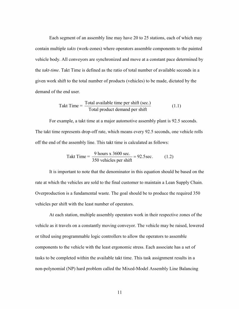
Each segment of an assembly line may have 20 to 25 stations, each of which may

contain multiple takts (work-zones) where operators assemble components to the painted

vehicle body. All conveyors are synchronized and move at a constant pace determined by

the takt-time. Takt Time is defined as the ratio of total number of available seconds in a

given work shift to the total number of products (vehicles) to be made, dictated by the

demand of the end user.

Total available time per shift (sec.)Takt Time =

Total product demand per shift (1.1)

For example, a takt time at a major automotive assembly plant is 92.5 seconds.

The takt time represents drop-off rate, which means every 92.5 seconds, one vehicle rolls

off the end of the assembly line. This takt time is calculated as follows:

9 hours x 3600 sec.Takt Time = 92.5sec.

350 vehicles per shift (1.2)

It is important to note that the denominator in this equation should be based on the

rate at which the vehicles are sold to the final customer to maintain a Lean Supply Chain.

Overproduction is a fundamental waste. The goal should be to produce the required 350

vehicles per shift with the least number of operators.

At each station, multiple assembly operators work in their respective zones of the

vehicle as it travels on a constantly moving conveyor. The vehicle may be raised, lowered

or tilted using programmable logic controllers to allow the operators to assemble

components to the vehicle with the least ergonomic stress. Each associate has a set of

tasks to be completed within the available takt time. This task assignment results in a

non-polynomial (NP) hard problem called the Mixed-Model Assembly Line Balancing

12

Problem which will be addressed separately in the Key Enabling Systems section of this

document. At the end of the assembly segment, there may be a quality check station that

focuses on critical assembly characteristics associated with the tasks completed in that

segment. At the end of the assembly segment, the vehicles get transferred across the

logistics aisle to the next segment to continue the assembly process. This process

continues along a serpentine sequence of conveyors until the entire assembly is complete.

After the assembly is complete, the vehicle is driven using its own power to the testing

area. All vehicles get driven into a booth that has a Dynamometer. The vehicle gets

accelerated to its maximum rated speed and a series of tests are done on the

Dynamometer. Finally the vehicle goes through a Road Test which includes driving it on

a specially developed surface prior to certifying the vehicle for final delivery.

2.1.5. Real-World Example of MMFA

The following data shows a typical range of values for key parameters that will

give readers feasible ranges of performance for a real-world Mixed-Model Automotive

Assembly (MMFA) line:

a. Takt time: 60 to 125 seconds

b. Assembly takts (multiple per station): 355 to 450

c. Labor per vehicle (Joining, Paining, Assembly) = 25 to 30 hours

d. In-process dedicated quality-check takts = 8 to 10

e. Available labor hours per shift = 8 to 10 hours

f. Vehicle built per shift (9 hours) = 260 @ 60 s. and 540 @ 125 s.

g. Takt time utilization = 92% - 96%

13

h. Number of mixed base models assembled on a line = 2 to 3

i. Number of variants of each base model assembled = 20 to 25

j. Number of optional sub-assemblies per variant = 300

Note: Takt time utilization for a given takt is the ratio of the sum of task times assigned to

the takt to the total available takt time. The range of the % utilization shown above is an

average utilization percentage across a typical automotive assembly plant. This metric

will be explained in greater detail in the Assembly Line Balancing section of this

document.

Multiple base models may be assembled on the same assembly line. For example,

a base model can be a small 5-seater Sports Utility Vehicle (SUV) and it can be

assembled alongside another base model which can be a 7-seater large SUV. Each of

these base models can have multiple variants such as Left-Hand Drive / Right-Hand

Drive, choice of 2.5 liter gasoline engine / 3.0 liter larger gasoline engine or a turbo-

charged diesel engine, or it can be a market specific variant that meets regulations of a

certain country where the vehicle will be shipped, and many others. We have observed

approximately 20 to 25 different variants per base model in a modern automotive

assembly plant.

Option content refers to the possible option choices that customers have when

they configure the vehicle. For example, a customer may be able to choose from up to 7

different roof-rails for a vehicle, depending on the selected variant.

The multiple base models, their variants, and the associated option content make

Mixed-Model Final Assembly a challenging multi-disciplinary problem.

14

2.1.6. Key Enabling Systems

Mixed-Model Final Assembly is feasible because the following key enabling

systems function seamlessly in the background:

Just-In-Time (JIT) Component Deliveries

The goal of Just-In-Time deliveries is to have the required components at the

required time in the required quantities in order to prevent accumulation. One of the

fundamental pillars of the Toyota Production System is Waste Elimination. Although

inspection, transportation, and storage of inventory are required elements of a

manufacturing process, only the actual processing is value added. JIT aims at eliminating

one of the primary waste sources which is storage of raw material and finished goods.

Mixed-Model Final Assembly reduces or practically eliminates finished goods

accumulation because the vehicles are produced just-in-time, directly based on the

customer orders and the same strategy is applied to the raw material receiving side.

Most automotive assembly plants that have implemented JIT deliveries have to

place a tremendous focus on schedule and capacity. Some companies allow customers to

place a completely customized vehicle order through a web-based configurator. These

orders are then sequenced in the form of a production plan and broadcast to the respective

vendors. On the other hand, some assembly plants operate on a sales forecast but divide

their schedule into several layers. The top level master schedule is based on extensive

market survey to estimate a relatively approximate demand for each model type. This

high level planning is used to plan capacities in the plant and raw material suppliers. This

estimate is given to the plants and vendors between 60 to 90 days in advance and firmed

15

up usually 30 days before the planned production date. The firm numbers are used for the

second level (weekly) and third level (daily) planning. A final leveled schedule is sent to

the final assembly line which drives the demand using the kanban system. Kanban is a

system of “pulling” components throughout the supply chain based on demand. Just-In-

Time (JIT) deliveries prevent inventory accumulation and thereby reduce the working

capital invested in inventory.

Instead of the long final assembly lines (Figure 2.6), the newer plants have a layout

like the fingers of a hand (Figure 2.7). Just like airport layout planners would like to

maximize the number of available gates, this floor layout allows the assembly plant to

have a significant number of dock doors all along the various fingers for JIT deliveries of

sub-assemblies and components directly at the point-of-use on the assembly line. This

minimizes the need to move racks over long distances from the dock doors to the point-

of-use, using forklifts.

16

Figure 2.7: "Finger-Layout” with more dock doors for JIT part supply

Single Minute Exchange of Dies (SMED)

In order to support a Mixed-Model Final Assembly line, the Just-In-Time

suppliers have to produce components in the same sequence as the final assembly line if

they wish to operate in a lean manner. This would require the ability to produce parts in

the same lot size (ideally one) as the Mixed-Model Final Assembly line. Another way to

support the final assembly line would be to maintain high stock levels of each variety of

supplied component and sequence it just before the components leave the supplier’s

dock. The latter alternative would be very expensive for the supplier due to very high

inventory holding costs and potential quality issues associated with stored components.

Most suppliers run a lean operation on the principles of Single Minute Exchange of Dies

(SMED), developed by Shigeo Shingo [4]. Following are some key definitions:

17

a) Changeover: A changeover or setup is a set of tasks that must be undertaken to

prepare the equipment to produce the next lot with a different part than the one

already produced. It also includes the tuning time that is required to adjust the

equipment to produce parts that meet the product specification.

b) Changeover Time: The total changeover time is defined as the time taken from the

last good part of component A to the first good part of component B that follows

component A in the production plan.

c) Single Minute Exchange of Dies (SMED): SMED is a theory and set of techniques

that make it possible to perform equipment setup and changeover operations in under

10 minutes.

This technique was first applied by Toyota to reduce the changeover time of

conventional press dies, hence the acronym SMED has the word “Dies”. Since then, the

basic principles have been applied to quick changeover across various processes beyond

conventional press dies but the original term SMED has continued to be applied. Also,

the term single refers to single digit time unit (less than 10 minutes).

Fundamentally, SMED is based on waste elimination and careful separation of

each and every changeover activity into two basic categories:

a) Internal Setup: Changeover activities that can be done only when the machine has

stopped producing parts and is shut down (e.g. the physical removal of the tooling

from the equipment).

b) External Setup: Changeover activities that can be done before the machine has

stopped producing parts, in preparation for the changeover (e.g. having all the tooling

18

available at the machine within the operator’s reach, rather than looking for it once

the machine stops producing parts).

The SMED activities can be divided into three major areas:

a) Distinguish Internal and External Setup Activities: This step includes a detailed

recording of every step of the changeover and careful evaluation of each step to

determine whether it is internal or external. An efficient way to carefully evaluate the

steps is to record the entire operation using a video camera. Then the analyst and the

experienced operator can review each step and note down the task, time required,

tools required, and whether it was internal or external. The advantage of recording the

entire changeover or setup is the ability to rewind and review the process as many

times as required to understand the operation clearly.

b) Convert Internal Activities to External: Once the difficult part of the process of

distinguishing between internal and external activities is complete, the most value

added process of converting internal to external activities begins. A checklist which is

very similar to a Bill of Material should be used to list every single tool, process

setting, and part specification to be maintained in the process. This checklist will

allow the operator to stage all the required components within arm’s reach from the

equipment to be changed over. An ideal technique to store these tools is by using a

Shadow Board ( Figure 2.8). It is a board that has a specific location for each tool

and an outline of the tool is drawn for each tool. That ensures that every tool has a

fixed place and every tool is in its place. If there is a “shadow / tool outline” that is

19

visible, it signifies a missing tool which helps the operator locate it before the

equipment is shut down for changeover.

Figure 2.8: Example of a Shadow Board

Another important part of converting the steps to external type is by staging the die

sets or tool that has to be physically changed over inside the equipment. Any time lost

in transportation after the machine has stopped producing parts would be categorized

as internal setup and accounts for lost time. An ideal staging technique in relatively

small machines is to have the tooling on a turn-table or turret so that it can simply be

turned by say 180 degrees and can be locked in place for operation. This will convert

all transportation time from internal to external. One final component of this process

is to simplify the adjustment required after the new tooling / die-set is installed in the

machine. Analysis of changeovers from a steel machining plant and a winder set

operation for a motor manufacturing plant shows that approximately 40% - 50% of

the total changeover time is attributed to adjustments that need to be made before the

first good part that meets specifications is produced. This is a significant contributor

to the internal setup which occurs after the machine has stopped producing parts.

20

Every second of adjustment time costs money and cannot be directly converted to

external setup like the transportation of dies or shadow boards for tool availability.

The only real way to reduce or eliminate this waste is by developing standardized

locating devices such as dowel pins and mistake proofing devices which allow only

one way to locate the parts. This eliminates the alternatives offered to the setup

technician and makes it simple. Use of limit switches and proximity sensors can also

be made wisely so that the technician gets a clear confirmation when the die-set or

tooling has been located in its correct position. The input from such devices can be

tied into the programmable logic circuit of the machine to prevent the machine from

cycling unless the tooling has been secured in the correct position. Such use of

mistake-proofing systems reduces the changeover time and it also reduces or

potentially eliminates scrap that is generated every time a new batch is run.

c) Standardize the Setup / Changeover operation: When tooling or components

related to a changeover are different, the operator has to make all those changes,

usually with the machine completely shut down. This would be considered a waste of

time as it is an internal set up and parts are not being produced. Those features that

are directly interacting with the fixture in which the die set gets located, should be

standardized. This also includes a set of standard shims that can be used to allow two

or more different die sets to work with the same clamp height and shut height.

21

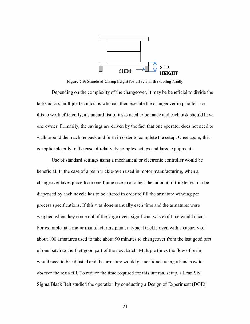
Figure 2.9: Standard Clamp height for all sets in the tooling family

Depending on the complexity of the changeover, it may be beneficial to divide the

tasks across multiple technicians who can then execute the changeover in parallel. For

this to work efficiently, a standard list of tasks need to be made and each task should have

one owner. Primarily, the savings are driven by the fact that one operator does not need to

walk around the machine back and forth in order to complete the setup. Once again, this

is applicable only in the case of relatively complex setups and large equipment.

Use of standard settings using a mechanical or electronic controller would be

beneficial. In the case of a resin trickle-oven used in motor manufacturing, when a

changeover takes place from one frame size to another, the amount of trickle resin to be

dispensed by each nozzle has to be altered in order to fill the armature winding per

process specifications. If this was done manually each time and the armatures were

weighed when they come out of the large oven, significant waste of time would occur.

For example, at a motor manufacturing plant, a typical trickle oven with a capacity of

about 100 armatures used to take about 90 minutes to changeover from the last good part

of one batch to the first good part of the next batch. Multiple times the flow of resin

would need to be adjusted and the armature would get sectioned using a band saw to

observe the resin fill. To reduce the time required for this internal setup, a Lean Six

Sigma Black Belt studied the operation by conducting a Design of Experiment (DOE)

22

and suggested the use of flow control valves with specific settings that were controlled

using programmable logic circuits. Several confirmation runs were conducted to study

the expected variation from batch to batch and once the process was confirmed to be

capable, the settings were recorded in the process control documents. After the changes

were implemented, a complete changeover could take place within 8 minutes and the new

batch would be loaded in the oven with only one empty collet between the two lots

signifying a changeover. This also eliminated the scrap associated with trial & error

based adjustments that were required prior to standardizing the resin quantities and the

flow control system.

In summary, Single Minute Exchange of Dies is a very effective technique to

reduce the actual down time of the machine during changeovers and setups. It includes a

systematic analysis of every step of the changeover, conversion of internal activities to

external activities, and finally standardization of the improved processes in order to

sustain the improvement long term. An overview of SMED has been included in this

section because several simple changeovers are part of the operator’s routine work as part

of the task. Such changeovers impact “Operator Choice Complexity” [5] which is based

on the probability of choosing the correct tooling and components. We capture this input

variable under human-factors in the generalized complexity model in Chapter 4.

2.2. Assembly Line Balancing

2.2.1. Introduction to Assembly Line Balancing (ALB)

The distribution of tasks among the work stations such that the precedence

constraints and possibly other restrictions are fulfilled, is called Assembly Line Balancing

23

(ALB). The high practical relevance of mixed-model assembly is also reflected by the

vast amount of academic research in this field. With only a few exceptions, the majority

of the numerous mixed-model assembly related research papers treat either one of the

following two planning problems:

1) The assembly line balancing problem constitutes a long-term to mid-term

planning problem, which seeks to group the total number of assembly

operations and assign them along with the required resources to the stations of

the assembly line.

2) The short-term sequencing problem of mixed-model assembly lines assigns all

jobs of the given production plan (model-mix) to the production cycles in the

planning horizon.

The balancing and the sequencing problem are heavily interdependent. While the

line balance decides on the assignment of tasks to stations and thus determines the work

content per station and model, the production sequence of a given model mix is arranged

on this basis with regard to minimum overloads. The amount of overload by itself is a

measure of efficiency for the achieved line balance. That is why some authors have

proposed a simultaneous consideration of both planning problems [6]. A simultaneous

approach is, however, only viable under special conditions as both planning problems

have completely different time frames, as explained above. Detailed forecasting of future

model sales are often bound to inaccuracies, especially if the assembled products are in

an early phase of their life cycle. It, thus, seems more meaningful to generally anticipate

24

the sequencing decision at the higher balancing level within a hierarchical planning

approach.

An assembly system performs a set of distinct minimum rational work elements

for the assembly of products and it consists of a set of work locations linked together by a

material handling mechanism and a detailed specification of how the assembly of the

product flows from one station to another. Following are definitions of basic terms and

the respective notation associated with Assembly Lines:

1) Task is a smallest indivisible work element n. Set 1,...,V n .

2) Station is a location along the flow line where the tasks are processed and it

consists of operators and/or equipment. Set 1,...,k m .

3) Performing a task j takes a task time tj and requires certain equipment and/or

operators.

4) The total workload necessary for assembling a work-piece is measured by the sum

of task times tsum.

5) The tasks cannot be assigned to stations arbitrarily because of technological

sequencing requirements, known as precedence relations. The processing of a

task may not start until certain tasks, i.e. its immediate predecessors have been

processed. The precedence relations are represented schematically by an acyclic

digraph called a precedence network/diagram whose nodes correspond to tasks

and if a task i is an immediate predecessor of task j (i.e., if the processing of task j

cannot start until after the completion of task i), this relation is represented by a

25

directed arc (i,j) in the precedence network/diagram, joining node i to node j. The

set of precedence relations is simply a partial ordering of the tasks.

6) The set Sk of tasks assigned to a station k constitutes its station load or work

content.

7) The cumulative task time ( )k

k jj St S t

is called station time.

8) A certain set of operations is performed repeatedly on a workpiece which enters

the station. The time span between two entries is referred to as cycle time. In a

paced line, the cycle time of all stations is equal to the same value c.

9) The series of stations and the material handling mechanism, usually a conveyor, is

referred to as the Assembly Line.

The decision problem of optimally partitioning (balancing) the assembly work

among the stations with respect to some objective is known as the assembly line

balancing problem (ALBP) [7].The first mathematical formalization of ALB was done by

Salveson [1]. When a fixed common cycle time c is given, a line balance is feasible only

if the station time of neither station exceeds c. In case of t (Sk) < c, the station k has an

idle time of c - t (Sk) time units in each cycle. In order to ensure high productivity, any

good balance should cause as few idle times as possible.

The basic ALBP can be distinguished into four types:

1) Type 1: For a given cycle time, minimizing the sum of station idle times is

equal to minimizing the number of opened stations.

2) Type 2: Conversely, if the number of stations is given, the minimizing the

cycle time guarantees minimum idle times.

26

3) Type 3: If both, number of stations and the cycle time, can be altered, the line

efficiency E is used to determine the quality of a balance. The line efficiency

corresponds to the productive fraction of the line’s total operating time tsum

and is typically defined as E = tsum/(m.c). As the total idle time is equal to tsum

- (m.c), a maximization of E also minimizes idle times.

4) Type 4: Finally, the problem of finding a feasible balance for a given number

of stations and a given cycle time falls under this category.

Figure 2.10 shows a precedence graph with n = 9 tasks having task times between

and 9 (time units).

Figure 2.10: Precedence Graph

The precedence constraints in Task 5 for example express that its processing

requires the tasks 1 and 4 (direct predecessors) and 3 (indirect predecessor) be completed.

The other way round, task 5 must be completed before its (direct and indirect) successors

6, 8, 9, and 10 can be started. Any type of ALBP consists in finding a feasible line

balance, i.e., an assignment of each task to a station such that the precedence constraints

and further restrictions are fulfilled. For the example in Figure 2.10, a feasible line

balance with cycle time c = 11 and m = 5 stations is given by the station loads S1 = {1,3},

27

S2 = {2,4}, S3 = {5,6}, S4 = {7,8}, S5 = {9}. While no idle time occurs in station load 2,

station loads 1, 3, 4, and 5 show idle times of 1, 2, 5, and 2 respectively.

Assembly Line Balancing involves task assignments to various takts in order to

maximize an objective such as Labor Utilization. Sequencing of tasks and Utilization are

both input variables in the generalized complexity model that we will review in Chapter

4. Our research shows that these have an impact on process driven complexity and can be

valuable input variables that can contribute in predicting product quality.

2.2.2. Manual Assembly Line Balancing

The study related to this research project was conducted at a major automotive

assembly plant on a pilot line where the electrical harnesses, floor insulation, and curtain

head airbags get assembled into the vehicle [8]. Typically, on a monthly basis, depending

on the change in model mix, the assembly team reviews the work distribution and

changes task assignment as needed, in order to maximize the labor utilization. The

current manual process of reviewing the various operations and rearranging the tasks to

improve the average utilization of the operators is labor intensive. To baseline the current

line balancing process, we (the author and his research team) participated in two line

balancing workshops. These workshops included the following steps:

Generate a visual display of all takts in the assembly line,

Analyze tasks that will exceed the cycle / takt time based on projected volume of

vehicles,

Re-balance each takt while ensuring that tooling / station / work zone constraints

are not violated,

28

Calculate the line utilization metrics,

Conduct trial runs to verify feasibility, and

Finalize the proposed line balance.

In each workshop, a cross-functional team was comprised of 5 experienced individuals

from assembly, Industrial Engineering, training, and quality departments. Distribution of

the average labor hours taken for this exercise is shown in Figure 2.11.

Figure 2.11: Distribution of Manual Line Balancing tasks (15 stations)

During the course of such a line balancing workshop that is typically done two

times per year, for each assembly line, each participant focuses 100% on the work

content evaluation and line balancing process. Tasks are manually arranged until the team

reaches consensus on the organization and then line trials are conducted. Similarly, on a

monthly basis, line gets re-balanced to account for the volume changes that have been

forecast for the following month. This exercise is usually done on a smaller scale than the

workshop described above, and includes 2 experienced associates who conduct the

planning and analysis in one day followed by line trials for two shifts. Although it seems

29

quite streamlined, this process relies heavily on the knowledge of the participants and

during the workshops it was evident that several constraints that should have been taken

into account were not easy to remember while making decisions manually, thereby

requiring multiple iterations to correct the issues that were found.

2.2.3. Constraints definition

Besides balancing a new assembly line, a running one has to be re-balanced

periodically or after changes in the production process or the production program have

taken place. Balancing means assigning the tasks to the stations (workplaces) based on,

among others, the precedence graph. In the automotive industry, typical information and

planning system contains the description of tasks including their deterministic task times

(derived by, for example a motion-time measurement MTM approach), the current

assignment of tasks to takts and the execution sequences of tasks within each takt.

However, almost no precedence relations are documented, not to mention an entire

precedence graph. The huge manual input and the multitude of tasks (up to several

hundreds or even thousands) prevent manufacturers from collecting and maintaining

precedence relations [9].

This absence of documented information on precedence relations is the main

obstacle in applying well explored theoretical assembly line balancing methods in

practice. In practice, planning, balancing and controlling assembly lines are based on

subdividing the production processes and, hence, the assembly lines into segments. Each

segment is managed by a dedicated human planner, who becomes an expert for this part

of the system. Though some software systems provide a component for automatic line

30

balancing, the planners mostly balance their segments of the line by manually shifting

tasks from one station to another, because precedence data is not available or existent

data is not reliable. This is a very time-consuming and fault-prone job, which is solely

driven by the experience and knowledge of planners. By appending the plans of

succeeding line segments, the entire production plan is developed.

This author along with his research group performed a pilot manual precedence

mapping exercise on an assembly trim (segment) comprised of 15 assembly stations at a

major automotive assembly plant where the roof rails, electrical harnesses, sub-woofer,

floor insulation, and curtain head airbags etc. get assembled into the vehicle [8]. The

primary purpose of this exercise was to understand the various constraints that would

need to be captured for the decision support system that would be the primary data source

for the optimization algorithm / construction heuristic. It was during this manual

constraints mapping exercise that the author observed that product quality could have an

impact based on the way tasks are arranged and therefore motivated the author to pursue

research related to manufacturing complexity, which includes several assembly line

related variables as key inputs.

In order to understand the process instructions and the actual work content, the

individuals who conducted this study underwent hands-on training on each assembly

station involved on the pilot line. The key advantages of conducting this training were as

follows:

1) Visualization of Process Instructions.

2) Understand precedence relationships.

31

3) Understand undocumented supporting tasks.

4) Gain basic understanding of additional complexity due to high option content.

5) Learn the effect of a work overload situation on operational metrics.

6) Awareness of the constraints that must be incorporated into the optimization

model.

7) Experience the ergonomic impact of repetitive tasks.

8) Understand the human behavior to adapt the required task to make it less

strenuous and more effective.

9) Gain input from assembly line associates based on their work experience.

After a thorough understanding of the tasks and the complexity, the

precedence mapping was manually undertaken in the following manner:

1) Stage 1: Each takt was evaluated to determine precedence relationships between

tasks within each takt.

2) Cross audit was conducted by multiple process experts to verify the precedence

relationships

3) Stage 2: Scope of the mapping exercise was expanded to the entire assembly line

and relationships were mapped across takts. In several cases, entire groups of

tasks were found to be predecessors of another group of tasks in a downstream

takt.

4) Data verification was done to ensure that cyclic relationships did not exist. A

cycle refers to a relationship that points from task i to j and another points in the

reverse direction, making j a predecessor for task i.

32

In addition to the basic task level precedence relationships, the following

constraints were identified and recorded during Stage 1 precedence mapping:

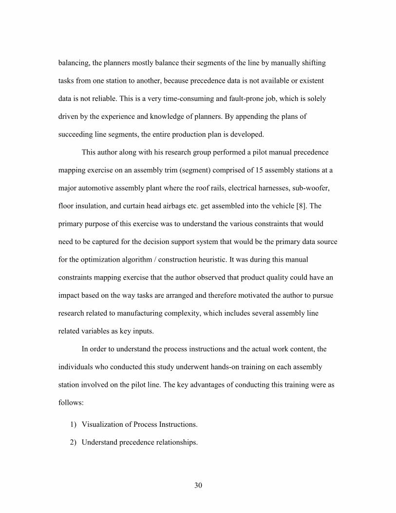
1. Product State constraint: The “Product State” can be defined as the physical

state in which the product gets presented at a certain assembly station (Figure

2.12).

Figure 2.12: Product orientation for ergonomics [8]

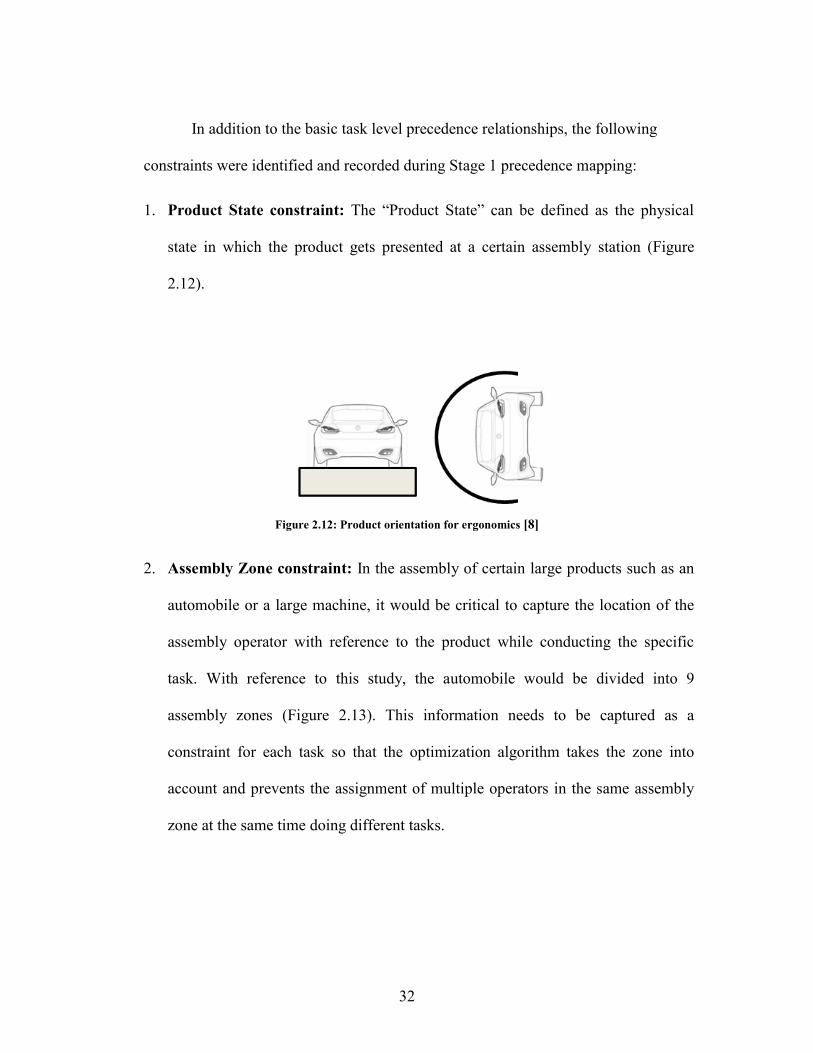
2. Assembly Zone constraint: In the assembly of certain large products such as an

automobile or a large machine, it would be critical to capture the location of the

assembly operator with reference to the product while conducting the specific

task. With reference to this study, the automobile would be divided into 9

assembly zones (Figure 2.13). This information needs to be captured as a

constraint for each task so that the optimization algorithm takes the zone into

account and prevents the assignment of multiple operators in the same assembly

zone at the same time doing different tasks.

33

Figure 2.13: Top view of product showing 9 assembly zones [8]

3. Ergonomic constraint: Every assembly task is assigned an ergonomic rating.

When tasks are not designed appropriately in systems that depend on human

operators, the system is particularly vulnerable to problems associated with

worker health, production, quality, and increased training costs. It is important to

capture this information as a constraint for the task distribution algorithm to be

able to set an objective to maintain the average ergonomic rating for a specific

assembly station below a pre-determined target.

4. Tooling constraint: During the precedence & constraint mapping exercise, it is

important to identify and record the specific tooling needed to execute a given

task (e.g., overhead lift assist systems). Moving such capital equipment is

expensive, so it should be kept at a certain station and included in the

optimization algorithm as a constraint.

The basic precedence mapping exercise required us to identify enabling

predecessors (tasks that need to be done before commencing the successor tasks). In

principle, as long as each one of those preceding tasks was completed, the dependent

task could be done, as shown in the battery installation example in Figure 2.14.

Figure 2: Top View showing 9 work zones(Source: www.wikicars.org)

34

Figure 2.14: Successor is independent of Predecessor Task Sequence [8]

However, in reality there are tasks that need to happen immediately after a

preceding task has taken place. For example, the windshield would needs to be

assembled immediately after the adhesive is applied. This presents a challenge in

terms of capturing the input data for the construction heuristic which is used for task

distribution, as the intent is not to treat the preceding tasks as independent tasks. If

treated independently, the task distribution process could potentially add several other

tasks between the adhesive application and the windshield assembly operation in

order to reduce idle time at each takt. From a process requirement standpoint, this

would be unacceptable. A possible solution would be to group such tasks to ensure

that they get executed in a sequence which would be pre-determined based on the

design or process requirements (Figure 2.15). Such grouping is considered as an

Adjacency Set. Another solution is to include time relations between tasks, such that

minimum and maximum separation between tasks can be enforced.

Figure 2.15: Task Grouping [8]

35

In summary, all these constraints were mapped for each takt during Stage 1 of

precedence & constraint mapping. Once the precedence relationships and constraints for

each takt were documented in Stage 1, the second stage included mapping the precedence

relationships between tasks, across takts. It was important to review process sheets that

had a detailed listing of every single task and the task time. The hands-on training was

very beneficial to visualize the tasks and identify predecessors from stations that were not

on adjacent stations.

The comprehensive precedence map which included Stage 1 and Stage 2 data was

then created using Microsoft® Visio software to review the precedence relationships in a

visual form. The visual representation was beneficial in highlighting circular references

or “floating” processes that did not have any predecessors. In some cases, a large cluster

of closely linked processes were found. This can occur when several small tasks such as

individual wire connections are done at a specific station. As long as they are part of a

sub-assembly (example, audio system), there was no additional advantage in trying to

split each small task and set the precedence relationships to the upper level task which

would in this case be the installation of the audio system. Instead it was found to be

beneficial to link each of these tasks as an adjacency set and link the very first one to the

preceding upper level task such as the audio system installation. This ensured that the

small tasks did not get fragmented during the task distribution process.

Although generating a line balance based on precedence relationships and the

above stated constraints could generate a potentially feasible sequence, an area not

36

explored by researchers is the impact of task sequencing and takt utilization on product

quality. A negative impact on product quality would certainly require the experts to

reverse the changes and re-balance the tasks. Therefore, in order to understand the impact

of Assembly Line Balancing on product quality, we include task sequence and takt

utilization as input variables in the complexity model, along with other variables that will

be explained in the following sections.

2.3. Complexity

2.3.1. Definition and previous work

Several scholars have attempted to define complexity at a manufacturing system

level with limited success. This is primarily because there are a large number of

contributors that prevent the functional objective from being achieved and depending on

the application; authors have focused on limited number of variables and defined them as

complexity drivers. A general definition of complexity is that a complex system is one

which has a large number of elements, whose relationships are not simple [10]. Whereas

static complexity describes the system structure at a defined point in time, dynamic

complexity represents the change in system configuration in the course of time [11]. In

order to understand how factors such as product variety, changing quality requirements or

varying customer demand regarding packaging, or delivery service complicate

manufacturing processes and in turn impact the performance of production systems, some

research work has been conducted mainly in the investigation of the static manufacturing

system complexity. Deshmukh et al. [12] derived an information-theoretic entropy

measure of complexity for a given combination and ratio of part types to be produced in a

37

manufacturing system. ElMaraghy et al. [13] proposed a code-based structural

complexity index to capture the amount of information in the manufacturing systems as

well as another complexity measure to represent the probability of a manufacturing

systems success in delivering the desired production capacity. Suh [14] defined

complexity in the context of manufacturing system design ‘as the measure of uncertainty

in achieving the functional requirements owing to a poor design or to the lack of

understanding and knowledge about the system’. Suh introduced the Axiomatic Design

(AD)-based complexity theory as a comprehensive approach to describe the mechanisms

of a manufacturing system’s static and dynamic complexity and illustrated the concept of

functional periodicity in a scheduling problem of a machine cluster to control the

system’s time-dependent combinatorial complexity.

The variety of products offered in mixed-model assembly lines has increased

dramatically over the past decade. For example, in a typical automobile assembly plant,

the number of different vehicles being assembled can reach tens of thousands in terms of

the possible build combinations of options. In fact, BMW claims that, “Every vehicle that

rolls off the belt is unique” and the number of possible automobile variations in the

BMW 7 Series alone could reach 1017

[5]. Such an astronomical number of build

combinations undoubtedly presents enormous difficulties in the design and operation of

the assembly systems. In the case of automotive assembly, it has been shown by both

empirical and simulation results [15, 16] that increased vehicle product variety has a

significant negative impact on the performance of the mixed-model assembly process, for

example, on quality and productivity. Such impact can result from assembly system

38

design as well as people performance under high variety. The effect from the latter

persists since only limited automation can be implemented in the automobile final

assembly [17, 18]. Thus, researchers have focused on this problem in two parts: how

variety impacts people and system performance, and how to design assembly systems and

organize production to allow high product variety without sacrificing quality and

productivity. One of the possible approaches to assessing the impact of product variety on

manufacturing system performance is to investigate how product variety complicates the

mixed-model assembly process. However, only limited research has been done on

defining manufacturing system complexity. For example, MacDuffie et al. [16]

established an empirical relationship between complexity and manufacturing system

performance. They defined product mix complexity by looking at product variety

(product mix and its structure) in assembly plants. According to the differences in the

levels of product variety, three types of product mix complexity were defined in terms of

empirical scores: model mix complexity, part complexity, and option complexity. The

result was based on the data from 70 assembly plants worldwide that participated in the

International Motor Vehicle Program at MIT [16]. Besides empirical studies, attempts

have also been made to analytically define complexity in manufacturing. For instance,

complexity has once been associated with the amount of effort needed to make a part.

The effort was quantified by a logarithmic function of the probability of achieving a

certain geometric precision and surface quality in machining [19].The function is widely

known as Shannon’s information entropy [20]. Similarly, Fujimoto and Ahmed [21]

defined a complexity index for assembling. The index takes the form of entropy to

39

evaluate the assemblability of a product. The assemblability was defined as the

uncertainty of gripping, positioning, and inserting parts in an assembly process. Also,

complexity has been extended as a measure of uncertainty in achieving the specified

functional requirements in an axiomatic design [22]. Recently, complexity has been

defined in an analytical form for manufacturing systems as a measure of how product

variety complicates the process. Fujimoto et al. [23] introduced a complexity measure

based on product structure using information entropy in different assembly process

planning stages. By reducing the complexity, they claimed that the impact of product

variety on manufacturing systems could be reduced. However, the complexity measure

does not incorporate the manufacturing system characteristics into the analysis.

2.3.2. Introduction to Axiomatic Design Principles [14]

Complexity theory based on Axiomatic Design (AD) was developed by Dr. Nam

P. Suh. Therefore, it is important to provide a brief background on Axiomatic Design.

AD theory is based on two fundamental axioms that eliminate the possibility of making

mistakes when products – both hardware and software, are developed. The theory helps

to overcome the shortcomings of the recursive product development process

(design/build/test), which requires continuing modifications as issues are found through

testing. There are several key concepts that are fundamental to AD. They are the

existence of domains, mapping, axioms, decomposition by zigzagging between the

domains, theorems and corollaries.

a. The concept of domains: The world of design is made up of four domains –

the customer domain, the functional domain, the physical domain, and the

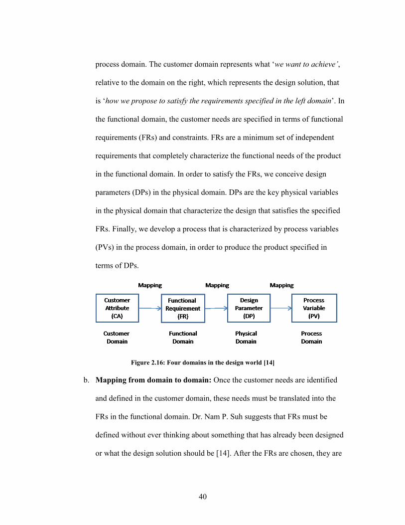
40

process domain. The customer domain represents what ‘we want to achieve’,

relative to the domain on the right, which represents the design solution, that

is ‘how we propose to satisfy the requirements specified in the left domain’. In

the functional domain, the customer needs are specified in terms of functional

requirements (FRs) and constraints. FRs are a minimum set of independent

requirements that completely characterize the functional needs of the product

in the functional domain. In order to satisfy the FRs, we conceive design

parameters (DPs) in the physical domain. DPs are the key physical variables

in the physical domain that characterize the design that satisfies the specified

FRs. Finally, we develop a process that is characterized by process variables

(PVs) in the process domain, in order to produce the product specified in

terms of DPs.

Figure 2.16: Four domains in the design world [14]

b. Mapping from domain to domain: Once the customer needs are identified

and defined in the customer domain, these needs must be translated into the

FRs in the functional domain. Dr. Nam P. Suh suggests that FRs must be

defined without ever thinking about something that has already been designed

or what the design solution should be [14]. After the FRs are chosen, they are

41

mapped into the physical domain to conceive a design with specific DPs that

can satisfy the FRs. For a given FR, there can be many possible DPs. The

right DP should then be chosen while making sure that other FRs are not

affected by the chosen DP and that the FR can be satisfied within its design

range.

Axioms: Dr. Nam P. Suh defines axioms as truths that cannot be derived but for

which there are no counter-examples or exceptions [14]. The basic postulate of AD

theory is that there are fundamental axioms that define acceptable designs. The two

axioms are: the Independence Axiom and the Information Axiom.

a. Independence Axiom: This axiom states that the FRs should be independent

of each other. When there are several FRs, the design must be such that FR

can be satisfied without affecting any of the other FRs. The relationship

between FRs is decided by the choice of DPs. It should be noted that FRs are

independent from each other by definition. Therefore, we have to choose a

correct set of DPs to be able to satisfy the FRs and maintain their

independence. After the FRs are established, the next step involves

conceptualization of the design solutions. This is a mapping process from

‘what’ in the functional domain to ‘how’ in the physical domain. When there

are many FRs, the design task may become difficult since the Independence

Axiom may be violated. The mapping process between the design domains

can be expressed mathematically in terms of two characteristic vectors as

follows:

42

FR DPA (1.3)

where A is called the Design Matrix that relates FRs to DPs and

characterizes the product design. Equation (1.3) is a design equation for the

design of a product. For a design that has three FRs and three DPs, the design

matrix is of the following form:

11 12 13

21 22 23

31 32 33

A A A

A A A A

A A A

(1.4)

Equation (1.3) may be written in a differential form as:

dFR dDPA (1.5)

where the elements of the design matrix are given by:

FR

DP

iij

j

A

(1.6)

For a linear design, As are constants; for a non-linear design, As are functions

of the DPs. There are two special cases of this design matrix:

1) The diagonal matrix, where all Aij = 0 except those where i = j.

11

22

33

0 0

0 0

0 0

A

A A

A

(1.7)

2) The triangular matrix as shown below:

11

21 22

31 32 33

0 0

0

A

A A A

A A A

(1.8)

43

For the design of processes involving mapping from the {DP} vector in the

physical domain to the {PV} vector in the process domain, the design

equation may be written as:

DP PVB (1.9)

where [B] is the design matrix that defines the characteristics of the process

design and is similar in form to [A]. To satisfy the Independence Axiom, the

design matrix must be either diagonal or triangular. When the matrix is

diagonal, each of the FRs can be satisfied independently and such a design is

called uncoupled design. When the matrix is triangular, the independence of

FRs can be guaranteed if and only if the DPs are determined in a proper

sequence. Such a design is called a decoupled design. Any other form of the

design matrix is called a full matrix and results in a coupled design. Coupled

designs are complex and cannot be decomposed readily because of the

complicated relationships among the FRs. Therefore, when several FRs must

be satisfied, designs must be developed in such a way that a diagonal or

triangular design matrix can be created.

b. The Information Axiom: This axiom states that the design with the

minimum information content is the best design. There may be many designs

that satisfy the Independence Axiom and the Information Axiom can be useful

in selecting the best among those designs.

44

The information content Ii for a given FRi is defined in terms of the

probability Pi of satisfying FRi:

2 2

1log logi i

i

I PP

(1.10)

The information content is expressed in bits of information. The logarithmic

function is chosen so that the information content will be additive, which is

useful when many FRs must be satisfied simultaneously.

In the general case of m FRs, the information content for the entire system Isys

is:

2logsys m

I P (1.11)

where P{m} is the joint probability that all m FRs are satisfied.

When all FRs are statistically independent, as is the case for an uncoupled

design,

1

m

imi

P P

(1.12)

then Isys may be expressed as:

2

1 1

logm m

sys i i

i i

I I P

(1.13)

When all FRs are not statistically independent, as is the case for a decoupled

design,

{ }1

for { }={1,..., -1}m

i ji

P m P j i

(1.14)

45

Where Pi|{j} is the conditional probability of satisfying FRi given that all other

relevant (correlated) {FRj}j=1,…,i-1 are also satisfied. In this case, Isys may be

expressed as:

2 |{ }

1

log for { }={1,..., -1}m

sys i j

i

I P j i

(1.15)

The Information Axiom states that the design with the smallest I is the best

design, since it requires the least amount of information to achieve the design

goals. When all probabilities are equal to 1, the information content is zero

and, conversely, the information content requires is infinite when one or more

probabilities are equal to zero. That is, if the probability is small, we must

supply more information to satisfy the FRs. Dr. Nam P. Suh’s Information

Axiom states that the FR must be satisfied within a specified range, which we

define as the design range [14]. The probability of success is governed by the

intersection of the design range defined by the designer to satisfy the FRs and

the ability of the system to produce the part within the specified range. The

probability of success can be computed by specifying the design range for the

FR and by determining the system range that the proposed design can provide

to satisfy the FR. To achieve a robust design, the system range should lie

inside the design range, thus reducing the information content to zero.

2.3.3. Complexity Theory based on Axiomatic Design [14]

One of the major goals of engineering is to reduce complexity of engineered

systems. Suh’s complexity theory based on AD provides a theoretical framework for

46

understanding and designing complicated systems. The theory gives guidelines for what

is possible and desirable in these systems.

Complexity is defined as a measure of uncertainty in achieving the specified FRs.

The complexity is measured in the functional domain rather than in the physical domain.

Complexity can be a function of time or can be independent of time. Therefore, it is

classified into two primary groups – Time-dependent complexity or time-independent

complexity.

Time-independent complexity consists of two different types: real complexity and

imaginary complexity. The information content defined by the Information Axiom is a

measure of real complexity. It measures how well the design satisfied FR, i.e. the overlap

between the design range and the system range. On the other hand, Imaginary complexity

is not real complexity but appears complex due to the lack of knowledge about the

design.

For a system range that changes as a function of time, there are two types of time-

dependent complexity: time-dependent combinatorial and time-dependent periodic

complexity. Combinatorial kind can lead to a chaotic situation if the number of

combinations continues to grow as a function of time. On the other hand, time-dependent

periodic complexity reduces the number of combinations to a finite set in a functional

period and may reduce the complexity problem to a deterministic one.

The introduction of functional periodicity into a system that has time-dependent

combinatorial complexity may substantially reduce the uncertainty of satisfying the FR.

Whenever a system with time-dependent combinatorial complexity is converted to a

47

system with time-dependent periodic complexity, uncertainty is reduced and the design is

simplified.

An example of time-dependent complexity is airline scheduling. If there is a

snowstorm at a hub airport that prevents airplanes from landing and taking off, other

airports will be affected. While the storm continues, the problem will get worse as time

passes. If the storm clears, the problem can be solved by reinitializing the system. It is

worth noting that as the airline schedule is periodic each day, all of the uncertainties

introduced during the course of a stormy day end after a 24-hour cycle. Such a time-

dependent complexity falls under the periodic complexity category.

2.3.4. Reduction of Complexity in Manufacturing Systems [14]

To make a system robust and reliable by satisfying the FRs and constraints

throughout the system’s life cycle, the complexity of the system should be reduced

starting from the design stage. Following are three primary ways of reducing complexity:

Elimination of time-independent real complexity by making the design robust

Elimination of time-independent imaginary complexity by writing the design

equation.

Transform time-dependent combinatorial complexity into a time-dependent

periodic complexity by introducing a functional periodicity.

The first step in introducing a functional periodicity is to decouple a coupled

system to make sure that the FRs can be satisfied independently and the system obeys the

Independence Axiom. For example, in the case of cellular manufacturing system,

processes are grouped according to the sequence and operations needed to make a

48

product [24]. The cell is designed in a U-shape so that the workers can move from

machine to machine, loading and unloading parts (Figure 2.17). The cell has one worker

who can make a walking loop around the cell in 110 seconds. The machines in the cell

have the capability to complete the desired processes untended, turning themselves off

when the machining cycle is complete. The cell usually includes all the processing

needed for a complete part or sub-assembly. If the machining time (MT) for a certain

operation is greater than the necessary cycle time (CT), that process needs to be

duplicated to ensure that MT < CT. By using multi-skilled operators, the need to balance

the line is eliminated as these operators are capable of operating multiple operations and

are motivated to provide support to every process in the cell that may need help. It is

important to note that between such processes, several different types of decouplers may

be placed. A decoupler may be designed to inspect the part before it gets picked up by the

next process and feed the information back to the previous machining step if any

corrective action is required. A decoupler may also help cool a heat-treated part before it

gets picked up by the operator for the next process step. Thus, a manufacturing cell

allows production of just enough parts to meet the production requirements without

generating additional inventory. Based on the principles of axiomatic design and

complexity reduction, functional periodicity is controlled in these cells by the removal of

the product from the last machine of a manufacturing cell. This is in contrast to having a

job shop type of a manufacturing system, where parts are pushed into the manufacturing

system as soon as a machine becomes available. In such a system, the parts are moved to

the next available machine. The number of combinations and permutations of processing

49

the parts through a set of processes in a job shop increases with time, thus constituting a

combinatorial complexity problem.

Figure 2.17: U-shaped cell with decouplers, [24]

2.3.5. Operator Choice Complexity

Variety has been shown to be a particularly important factor in error frequency.

Gatchell [25] observed that operators with a choice of 10 parts made 46 percent more

50

errors and needed 13 percent more decision time than operators who could choose from

only 4 parts. In Zhu et al. [5] the variety induced manufacturing complexity in manual

mixed-model assembly lines is considered where operators have to make choices for

various assembly activities. The authors propose a complexity measure called ‘operator

choice complexity’ to quantify human performance in making choices. Operator choice

complexity is defined as the average uncertainty or randomness in a choice process,

which can be described by a function H in the following form (2.1):

1 2

1

( ) ( , ,..., ) logM

m m m

m

H X H p p p C p p

(2.1)

Where, C is a constant depending on the base of the logarithm function chosen. If log2 is

selected, C=1 and the unit of complexity is bit.

There is a close similarity and connection between the theoretical properties of the

complexity measure and the experimental results found in human cognitive studies. The

experiments were conducted to assess human performance when making choices.

Coincidentally, information entropy was found to be one of the effective measures. The

performance of human choice-making activities was investigated by measuring average

reaction times (RTs), i.e., how quickly a person can make a choice in response to a

stimulus. One of the earliest studies was done by Merkei in 1885, described by

Woodworth [26]. In the experiment, digits 1–5 were assigned to the fingers of the right

hand and the Roman numbers I–V were assigned to the fingers of the left hand. On any

given set of trials, the subject knew which of the set of stimuli would be possible (e.g., if

there were three possible stimuli, they might be 3, 5, and V). Merkel studied the

51

relationship between the number of possible stimuli and the choice RT. His basic findings

are presented in Figure 2.18, where the relationship between choice RT and the number

of alternatives was not linear. This relationship in Figure 2.18 has been further studied by

a number of researchers since Merkel’s original observations.

Figure 2.18: Mean choice RT vs. stimulus-response alternatives [26]

Among them, the most widely known one was Hick [27]. He discovered that the choice

RT is linearly proportional to the logarithm of the number of stimulus alternatives if all

the alternatives are equal (Figure 2.19), i.e.,

2Mean choice [log ]RT a b n (2.2)

52

Where, n is the number of stimulus-response alternatives, and a and b are constants,

which can be determined empirically by fitting a line to the measured data. This relation

came to be known as Hick’s law, which was regarded as one major milestone in the

area of cognitive ergonomics.

Figure 2.19: Mean choice RT as a function of log of the # of alternatives [27]

Coincidentally, the term (log2 n) is exactly the information entropy calculated in (2.1) if

all the pm’s are equal, which follows from the experiment setting that the choice process

is iid (independent and identically distributed) and all the alternatives likely occur

equally. The above analogy was first discovered by Hyman [28], where he concluded that

“the reaction time seems to behave, under certain conditions, in a manner analogous to

the definition of information.” Hyman also realized that, according to Shannon’s

definition of information entropy, he could change information content in the experiment

53

by other means. Thus, in addition to varying the number of stimuli and letting each one of

them occur in Hick’s [27] experiment, he altered stimulus information content simply by:

Changing the probability of occurrence of particular choices

Introducing sequential dependencies between successive choices of alternatives

(Figure 2.20).

Figure 2.20: Choice RT vs. stimulus information H [27]

Thus, we can use H to replace the (log2 n) term; (2.2) becomes:

Mean choice RT a bH (2.3)

Because of the significance of this generalization, Hick’s law is also referred to as the

Hick–Hyman law. The H term in the above equation is one of the variants of Shannon’s

information entropy [20] in the communication systems study. Thus, a fundamental

assumption behind this analog is that the mental process of a human being is modeled as

an information transmission process. Liu [29] suggested that at a level of mean RTs, a

continuous-transmission fork-join network demonstrates the same logarithmic behavior

54

as that of experimental results in the Hick-Hyman law. Hence, the legitimacy of applying

this equation is limited to situations where individuals are asked to respond promptly to a

stimulus, and the decision to be made is very simple, requiring little conscious thought. In

mixed-model assembly process, we observe a very similar situation that the line

associates are asked to handle variety in a very tight cycle time without time for

deliberating over the decisions.

2.3.6. Cognitive Load Theory

Cognitive Load is closely linked to the Operator Choice Complexity described

above. The objective of cognitive load theory (CLT) is to predict learning outcomes by

taking into consideration the capabilities and limitations of the human cognitive

architecture [30]. The theory can be applied to a broad range of learning environments

because it links the design characteristics of learning materials to principles of human

information processing. CLT is guided by the idea that the design of effective learning

scenarios has to be based on our knowledge about how the human mind works. Starting

from this premise, different processes of knowledge acquisition and understanding are

described in terms of their demands on the human cognitive system, which is seen as an

active, limited-capacity information processing system. Taking into account the demands

on cognitive resources induced by the complexity of the information to be learned, the

way in which the instruction is presented to the learner, and the learner’s prior experience

and knowledge, CLT aims to predict what makes learning successful and how learning

can be effectively supported by teaching and instruction. A growing body of empirical

research has become available in recent years that describes the relationships among

55

human cognitive architecture, the design of educational materials, and successful

learning. Moreover, the research conducted in past years has led to a more detailed

description of the theoretical components of CLT, including processes of schema

acquisition, capacity limitations, and different causes for load, namely, intrinsic load

(generated by the difficulty of the materials), extraneous load (generated by the design of

the instruction and materials), and germane load (the amount of invested mental effort).

In mixed-model automotive assembly lines, instruction about the option content

to be assembled in a specific vehicle is relayed to the operator in multiple different ways:

56

Bar-coded broadcast sheet placed on the vehicle body (Figure 2.21).

Visual display screen triggered by the radio frequency (RF) device on the

vehicle (Figure 2.22).

Audio device coupled with the visual display to reduce the need for the

operator to look at the screen to determine the option to be chosen.

Figure 2.21: Broadcast sheet on vehicle (BMW, Leipzig)

57

Figure 2.22: Visual display of options to be installed in a specific vehicle

In summary, several researchers have attempted to define complexity at a

manufacturing system level. We now turn our attention to Automotive Assembly Quality

before focusing on the correlation between Manufacturing Complexity and Quality.

2.4. Introduction to Automotive Assembly Quality

Buzzell et al [31] proclaimed that “Quality is King”, affirming its dominant role

in market share and Return on Investment (ROI). The principle measure of Conformance

Quality for products, as described by Garvin [32] is product yield in terms of defects

generated by the manufacturing process. In the Automotive industry, quality has become

increasingly important as customers have several alternatives to choose from the

marketplace. Market research firms such as J. D. Power routinely measure number of

defects per 100 vehicles and publish the results. This survey is constructed to reflect only

those defects that an assembly plant can affect, i.e. omitting defects related to the

58

powertrain, while emphasizing defects related to the fit and finish of body panels, paint

quality, and the integrity of electrical connections. On the other hand, Consumer Reports

publishes reliability ratings for vehicles so that customers can evaluate the long term

reliability of sub-systems inside the vehicle. Such readily available information has made

vehicle manufacturers step up their internal quality measures and tie those metrics to

ensure that the customer is delighted when he/she receives the delivery of a brand new

car and more importantly to ensure that the customer stays loyal by enjoying the

performance of the vehicle along with robust reliability. Several concepts and methods

have evolved with the goal of improving conformance quality. Following is a brief

review of the conventional quality control methodologies that are being used for the last

several years and their respective limitations:

2.4.1. Statistical Process Control (SPC)

In virtually all manufacturing processes, the dimensions and quality of individual

parts needs to be known and controlled to meet design specifications. If such dimensions

are not controlled, costly delays and failures may result. Inspection strategy can fall into

one of the three following categories:

a. 100% inspection: Each and every part can be measured, manually or by some

automated method

b. Sampling: Some portion of the output can be measured by taking a sample lot of

parts at a certain frequency

c. No inspection: Under the assumption that everything that is manufactured meets

required specifications, none of the parts get inspected

59

Usually, manufacturers choose one of the first two categories depending on the risk

associated with a defective part. Sampling strategy involves looking at a certain

percentage of the entire population of parts using statistical techniques. This is known as

Statistical Process Control (SPC). The basic SPC techniques are the histogram and

control charts. The x-axis would represent various ranges of a dimension (e.g. a shaft

length) and the y-axis would represent the frequency at which these measurements were

found. The natural process limits of the measured distribution can be compared with the

engineering specifications to determine if the process is centered at the nominal value or

requires an adjustment. The location of the tails of the histogram with reference to the

design specification limits for a given dimension would show whether the parts being

produced are within specification or a small population does not meet the requirements.

Control charts for variables are used to monitor the output of a process by sampling, by

measuring selected quality characteristics, by plotting the sample data on the chart, and

then by making decisions about the performance of the process. Three common types of

charts that are used in typical manufacturing processes are:

1) X-bar chart: This chart tracks the aim / target (accuracy) of the process

2) R chart: The range chart tracks the precision or variability of the process

3) σ chart: The σ chart is used in place of R chart if the sample size is large

It is important to know that sampling errors can occur. Two kinds of decision errors are

always possible:

1) Type I error: If the process is running well but the sample data indicates that an

adjustment is required

60

2) Type II error: Contrary to the Type I error, in this type the sample data fails to

indicate that something is wrong with the process, when indeed an adjustment is

required

Many manufacturing companies determine the size of the errors they are willing to accept

according to the financial loss associated with making the error plus the cost of

inspection.

This conventional quality control method has two major shortcomings:

1. This method is reactive by nature. When the point of detection is downstream

from the defect source, the delay in responding to a process variation can

result in a significant number of defects.

2. SPC focuses on the manufacturing process and does not take product design

into consideration. Although manufacturing process control plays a big role,

several defects are caused due to a product design issue and this method does

not take focus on the design.

2.4.2. Taguchi’s Robust Design

In contrast with the reactive SPC technique, Taguchi’s Robust Design considers

defect issues relative to the product design as well as the manufacturing process. Quality

Engineer – Genechi Taguchi must be credited with much of today’s interest in the use of

factorial and fractional factorial designs on the part of the automotive and assembly

industries [33]. Within these industrial environments, experiments are run to identify the

settings of both product design parameters and process variables that will simultaneously

provide a manufactured item whose response is robust to process variability while

61

meeting the customer’s product expectations and possible environmental challenges. The

adaptation of statistical experimental design to these objectives has its origins in

Taguchi’s early work in the communications industries in Japan in the 1950s. The

strategy is called “parameter design” or “robust design”. The word “design” takes

different connotations: product design, process design, and statistical design.

A product’s response y is considered to be a function of “controllable” factors x

and the “noise” factors z. The objective is to choose settings of x that will make the

product’s response y insensitive to variability associated with both x and z and still meet

target specifications with least variability.

2.4.3. Six Sigma and Process Capability

Six Sigma methodology seeks to reduce or eliminate defects caused by variation

by assuring that design requirements have been established correctly in the design phase

and that the manufacturing process capability meets these requirements. An important

measure used in the Six Sigma methodology is the Process Capability index (Cp). For

bilateral tolerances, this index is defined as:

| | Tolerance width

6 Process capabilityp

USL LSLC

(2.4)

Where,

USL = Upper Specification Limit

LSL = Lower Specification Limit

Standard Deviation of the production process

62

The process capability index can be used to predict how frequently the outcome of a

process will exceed specification limits. This is a useful tool but focuses only on the

design tolerances and ability of the process to manufacture parts consistently within those

specifications. One of the drawbacks of analysis using these tools is that most quality

engineers focus on the primary distribution followed by the data. For example, the data

for a process could be normally distributed. In most cases, the tails of the distribution are

not part of the consideration except for the defect rate estimation in Parts per Million

(PPM). Understanding the nature of rare events and the limitations of statistical methods

is particularly important when the goal is to achieve near-zero defect levels.

2.4.4. Self and Source Inspection

Shigeo Shingo has introduced several quality concepts that overcome some of the

limitations of other methods. Self-inspection and source inspection have the goal of

detecting and eliminating defects at their production source [34]. Self-inspection has the

objective of detecting defects as close to the point of origination as possible or to reduce

delays in feedback. By gauging tools, materials and activities upstream of the process, it

is possible to eliminate any defects before they are created, using source inspection.

However, like SPC, these methods are manufacturing focused and do not address design

issues.

2.4.5. Pokayoke and 100 % Inspection

Shigeo Shingo makes an important distinction between human error and product

defects. While errors are inevitable, defects are not. He has stated [34]:

63

“We should recognize that people are, after all, only human and as such, they will, on

rare occasions, inadvertently forget things. It is more effective to incorporate a checklist,

i.e. a pokayoke device into the operation so that if a worker forgets something, the device

will signal that fact, thereby preventing defects from occurring. This, I think, is the

quickest road leading to attainment of zero defects.”

Similarly, Rasmussen [35] concluded that the frequency of error derived from

defect reports is dependent on the opportunity for people to detect and correct the errors

immediately. No amount of vigilance or training will assure that unintentional errors will

be recognized. Use of pokayoke is required to catch every single error and result in a

defect free output. Using pokayoke devices, defect probabilities will be less than error

probabilities. Consequently, defects are more likely to be related to the level of quality

control than to the frequency of errors. Therefore, centering attention on error prevention

and intervention is more productive than prediction of error rates for manufacturing

problems.

In some cases, pokayoke has been incorporated in the design process, thereby

preventing incorrect assembly [36]. However, pokayoke devices are generally used on

the assembly line to prevent assembly defects rather than an available technique that can

be incorporated into the product design.

2.5. Correlating Complexity and Quality

Efforts associated with manual precedence graph generation at a major

automotive manufacturer have highlighted a potential relationship between

manufacturing complexity (driven by product design, assembly process, and human

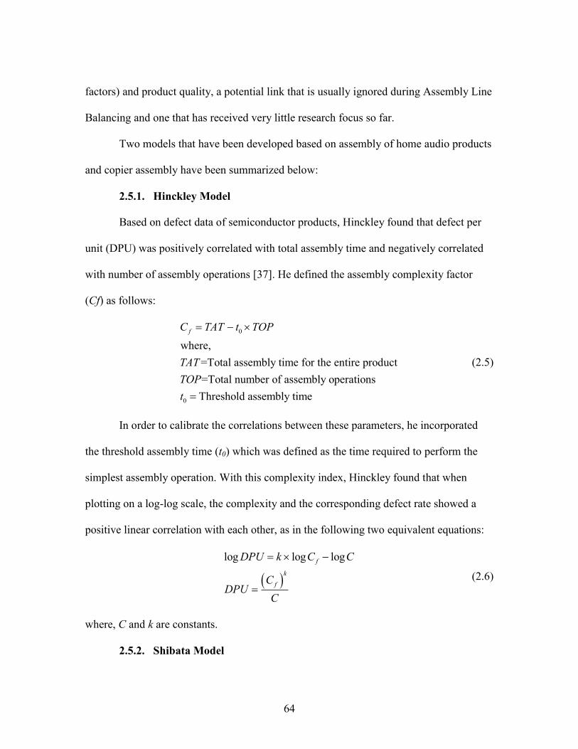
64

factors) and product quality, a potential link that is usually ignored during Assembly Line

Balancing and one that has received very little research focus so far.

Two models that have been developed based on assembly of home audio products

and copier assembly have been summarized below:

2.5.1. Hinckley Model

Based on defect data of semiconductor products, Hinckley found that defect per

unit (DPU) was positively correlated with total assembly time and negatively correlated

with number of assembly operations [37]. He defined the assembly complexity factor

(Cf) as follows:

0

0

where,

=Total assembly time for the entire product

=Total number of assembly operations

Threshold assembly time

fC TAT t TOP

TAT

TOP

t

(2.5)

In order to calibrate the correlations between these parameters, he incorporated

the threshold assembly time (t0) which was defined as the time required to perform the

simplest assembly operation. With this complexity index, Hinckley found that when

plotting on a log-log scale, the complexity and the corresponding defect rate showed a

positive linear correlation with each other, as in the following two equivalent equations:

log log logf

k

f

DPU k C C

CDPU

C

(2.6)

where, C and k are constants.

2.5.2. Shibata Model

65

Shibata [38] remarked that the Hinckley model did not take the assembly design

factors into consideration and could not evaluate the defect rate for a specific

workstation. Therefore, Shibata proposed a prediction model for a workstation based on

two assembly complexity factors: the process-based complexity factor and the design-

based complexity factor. Assembly time was determined by Sony standard time, a

commonly used time estimation tool for electronic products. Shibata used home audio

products, a combination of CD player and a MiniDisc recorder/player as assembly cases.

These had approximately 300 job elements and the total time was approximately 10

minutes.

The process-based complexity factor of workstation i is defined as:

0

1

0

.

where,

=number of job elements in workstation ;

time spent on job element in workstation ;

threshold assembly time

aiN

Pi ij ai

j

ai

ij

Cf SST t N

N i

SST j i

t

(2.7)

Shibata used Sony standard time (SST), a commonly used time estimation tool,

which is based on field studies and statistics. Home audio equipment served as a good

vehicle for Shibata’s analysis because its assembly process contained almost every type

of basic assembly operation that is present in consumer electronic products.

Similar to the Hinckley Model, Shibata derived the following correlation between

the process-based assembly complexity factor and DPU:

logDPU .log logi PiK Cf C (2.8)

66

DPU

K

Pi

i

Cf

C (2.9)

where C and K are constants.

In addition to the process-based complexity, Shibata defined the design-based assembly

complexity factor as:

DDi

i

KCf

D (2.10)

where, KD is an arbitrary coefficient for calibration with process-based

complexity; Di is called the ease of assembly of workstation i, evaluates based on the

method of design for assembly/disassembly cost-effectiveness (DAC) developed in Sony

Corporation.

Shibata found that the correlation between the design-based complexity and DPU

can be expressed as follows:

DPU .

log(DPU ) .log( ) log

b

i Di

i Di

a Cf

b Cf a

(2.11)

where, a and b are constants.

In response to the above model, Mendenhall and Sincich suggested that more

independent variables can improve the accuracy and stability of the regression function.

Shibata derived a bivariate prediction model by combining (2.8) and (2.11):

1 2log DPU . log .logi Pi Dik Cf k Cf C (2.12)

Su et al. [37] used the Shibata model to predict quality defects in a copier

assembly operation and found the value of R-square in the regression model to be 0.257

67

versus a value of 0.7 reported by Shibata for the home audio products. This proved that

the Shibata model was not appropriate for electromechanical products like copiers. One

of the primary reasons was the fact that Sony standard time had a threshold assembly

time of 2 seconds vs. 0.6 seconds in the case of the copier assembly.

Following is a brief description of additional work that has been done by

researchers to correlate certain elements of a manufacturing system with quality:

2.5.3. Relationship between Ergonomics and Quality

Knowledge from research or practical evidence, of the relationship between

ergonomics and quality is limited [39]. The literature contains a large number of studies

showing clear relationships between poor lighting, noise, unfavorable climatic conditions

and the effects on people’s work in terms of increased error frequency. It has been

observed that systematic quality work, as in quality circles for example, is also a method

that can solve working environment problems [40]. Eklund [41] conducted a

comprehensive study in a Swedish car assembly plant. The most physically demanding

tasks, the tasks with the most difficult parts to assemble, and the most psychologically

demanding tasks, were identified by interviews with experienced assembly workers.

Designs involving difficult assembly accounted for the largest proportion of quality

deficiencies, and psychologically demanding tasks showed the smallest proportion. The

results showed that the quality deficiencies were three times as common for the work

tasks with ergonomic problems, compared with other tasks. A quantifiable relationship

using standardized ergonomics metrics and product quality has not been published.

2.5.4. Associate Training

68

Associate training plays an important role in the complexity model. Hancock et al

[42] did not correlate training with resulting quality but demonstrated that the cycle time

per task decreases as experience, measured by the number of repeated cycles (x),

increases. They described this phenomenon as the “Learning Curve” which has the form:

L

x

KY

x (2.13)

where,

=cycle time per task for the cycle

K=the time for the first cycle, and

a constant determined by the learning rate (usually 0.80)

th

x

L

Y x

2.5.5. Human Error

Although some authors have touched the topic of human error and variation, this

distinction has not been accurately described in the literature. This is probably due to the

fact that it is virtually impossible to accurately assess rare events using sampling

methods. There are many types of error that can occur in an operation. While each of

these are individually rare occurrences, collectively they can have a significant impact on

conformance quality. Harris [43] concluded that 80 percent of the defects in complex

systems could be attributed to human error. In an examination of 23,000 assembly

defects, Rook [44] found that 82 percent of the defects were caused by human errors.

Voegtlen [45] reported that 60 percent of product failures could be traced to

workmanship defects. A recent study of automotive headlamps also showed that more

than 70 percent of 6,600 observed defects were caused by assembly or handling errors.

These studies point to human error as a significant contributor to the total defects.

69

2.5.6. Component & Assembly Quality

The National Research Council [46] study presented a combinatorial model of

defects. This method of combining the probability of many independent events is the

basis for all modern reliability evaluations and essential element of a sound defect model.

Two useful defect categories are: part defects and assembly defects.

A part may contain material defects, or may not meet functional requirements due

to variation or errors in processing or material handling. Variation can be due to process,

gage response, tool wear, operator error, and multiple such factors. Hinckley [47] defined

the probability of a part defect in the simplest terms consistent with the NRC model as:

{ part is defective}=

0 1

th

i

i

P i d

d (2.14)

Errors such as omitting a part, installing a wrong part, or placing the part in an

incorrect orientation will result in defects. Several studies have shown that there is a

correlation between an increased probability of an error and difficulty / time required to

execute a task [48, 49].

Given that assembly operation involves the addition of a part, the part could

contain a defect, the assembly operation could cause a defect, or both the part and

assembly operation could result in defects. Thus, there are three separate ways of

introducing one or two defects into a product when assembling a part. By contrast, there

is only one way of having a defect free assembly – the part must be defect free and the

assembly operation must not result in a defect. As a result, calculating the probability that

an operation does not introduce a defect is much easier than calculating the probability

70

that it will cause a defect. Thus yield would basically be a combination of the two

probabilities: the probability that the part is defect free and that the assembly operation

did not result in a defect.

2.5.7. Task (Assembly) Time and Quality

In late 1990, Brannan [50] at Motorola published the data shown in Figure 2.23,

which demonstrated that the number of defects per million parts decreased dramatically

for increases in the manual assembly efficiency, an arbitrary measure used in the

Boothroyd Dewhurst® [51] Design for Assembly (DFA) method.

Figure 2.23: Observed DPMO vs. the Manual Assembly Efficiency [50]

In general, as the assembly efficiency increases the number of assembly

operations and the average time required to perform each operation decreases. Assuming

a constant probability of human error per unit time, the defect rate should increase as the

assembly time per operation or complexity increases. Thus, the relationship between

defects and assembly efficiency observed by Motorola is intuitively sound, but was not

explained at the time. The data provided by Motorola suggested that there may be a

quantifiable link between a criterion describing assembly complexity and product defects.

71

Such a theory could be used to evaluate the product quality of product concepts even

before tolerance studies are initiated.

The Boothroyd and Dewhurst evaluation centers on establishing the cost of

handling and inserting component parts [52]. Regardless of the assembly system, parts of

the assembly are evaluated in terms of, ease of handling, ease of insertion and a decision

as to the necessity of the part in question. From this, time and cost is generated for the

assembly of that part. Each part is entered into the worksheet. The first stage analysis is

an attempt at part reduction. Each part is examined with respect to the following

questions:

1) During operation of the product, does the part move relative to all other parts

already assembled? Only gross motion should be considered; small motions

that can be accommodated by elastic hinges, for example, are not sufficient

for a positive answer.

2) Must the part be of a different material in order to be isolated from all other

parts already assembled? Only fundamental reasons concerned with material

properties are acceptable.

3) Must the part be separate from all those already assembled because otherwise

necessary assembly or disassembly of other separate parts would be

impossible?

The Design for Assembly (DFA) methodologies have been used by Barkan et al.

[53] to predict assembly complexity using assembly time as a standard. They have shown

that the predicted times are superior to the simplistic measures such as number of

72

components to be assembled and number of assembly operations. In general, for every

factor that increases the difficulty of the action or the complexity of the assembly

interface, there is an increase in the predicted time for execution. This approach is an

evolution of Time and Motion studies that substantiate the general trend of increased

execution time for increases in the difficulty and complexity of the assembly task. The

DFA methods are better than the Predetermined Motion Time Systems (PMTS) for

assessing assembly complexity because they are more directly related to product

characteristics than production planning. Additionally, the DFA analysis can be done

using drawings, without having to physically disassemble products or define each

assembly motion. The databases and rules of use encourage a more consistent

interpretation than can be achieved in a conventional tear-down analysis suggested by

Womack [54].

2.6. Summary of Background Work

In this chapter we provided a brief overview of the automotive manufacturing

processes and mixed-model final assembly along with an introduction to key-enabling

systems for MMFA. We also reviewed the Assembly Line Balancing Problem,

constraints definition and a method of manually gathering that information to solve the

problem. This manual exercise highlighted a potential link between manufacturing

complexity and product quality. We then provided a literature review on Complexity,

Axiomatic Design principles, Operator Choice Complexity, and Cognitive Load Theory.

This section was followed by a brief overview of the common methods to control quality

in manufacturing plants. Finally, the last section in the chapter focused on previous work

73

related to correlating Complexity and Quality. Researchers, Hinckley and Shibata

focused on developing a global model for assembly complexity and product quality based

on analysis of semiconductors and home audio appliances.

In the following chapters, gaps in the currently published research work will be

highlighted, followed by definition & development of a general complexity model and

finally it will be applied to a controlled fastening process in a real-world mixed-model

automotive assembly plant.

74

CHAPTER THREE

3. GAPS IN CURRENT WORK AND RESEARCH PLAN

3.1. Research Objective

The objective of this research is to test the hypothesis that manufacturing

complexity can reliably predict product quality in mixed-model automotive assembly.

3.2. Research Gaps

Several scholars have attempted to define complexity at a manufacturing system

level with limited success. This is primarily because there are a large number of

contributors that prevent the functional objective from being achieved and depending on

the application; authors have focused on limited number of variables and defined them as

complexity drivers. In order to reliably predict quality based on manufacturing

complexity, we need to take into account an array of input variables that have the ability

to statistically account for the variation in the resultant variable (product quality).

Focusing on a few individual variables and prove that they have some impact on product

quality would not be adequate in achieving the objective of this research.

Seminal work in this area has been done by Hinckley [47], Shibata [38], and Su

et. al. [37].

The research gaps in the work done by these researchers are summarized as

follows:

1) Hinckley’s Model [47]: The mathematical model is as follows:

0Cf TAT t TOP (2.15)

75

0

where,

Assembly Complexity factor

Total assembly time for entire product

Threshold assembly time

Total number of assembly operations

Cf

TAT

t

TOP

log DPU = .log log

( )DPU =

K

k Cf C

Cf

C

(2.16)

where,

DPU = Defects per unit

& = ConstantsC K

Though this model enables us to grasp schematically the relative level of quality

control among globally distributed manufacturing sites, a major shortcoming of

the model is that it only reveals the product quality at an overall plant level. The

model does not take the assembly design factors into consideration and could not

evaluate the defect rate for a specific station. It does not assess process level

complexity and its impact on quality. In order to reduce complexity, designers

would need to know which part design produced increased levels of assembly

complexity resulting in assembly defects. Also, Hinckley’s model takes into

account average assembly time and the threshold assembly time but does not take

into account variation in assembly times, an important input for the complexity

model that we found based on our study. We discuss this in chapters 4 and 5.

In order to validate the model in the automotive assembly environment for

total DPU, we used a simple example as shown below:

76

Table 3.1: Application of Hinckley Model to Vehicle Assembly

Although the total assembly time is higher in the case of Model A, and the

threshold time is 4 seconds, the complexity factor Cfpi is inversely proportional to

the total assembly time and DPU (Figure 3.1). This contradicts the finding that

Hinckley had when they applied it to semiconductor manufacturing which was

perhaps a lot more repetitive in tasks as compared to automobile assembly tasks.

Figure 3.1: Hinckley Model validation

2) Shibata’s Model [38]: In contrast to a model based on global manufacturing

plants that provides a high level overview of a correlation between complexity

77

and product quality, Shibata considered process and design contribution in the

research. Following is the mathematical formulation of the Shibata Model:

0

1

.aiN

Pi ij ai

j

Cf SST t N

(2.17)

0

where,

Process based complexity factor

# of job elements in workstation

Time on job element in workstation

Threshold assembly time

pi

ai

ij

Cf

N i

SST Sony j i

t

DDi

i

KCf

D (2.18)

where,

Design based complexity factor

Coeff. for calibration with

Ease of assembly cost-effectiveness ( )

Di

D pi

i

Cf

K Cf

D Sony

1 2log DPU = .log .logi pi Dik Cf k Cf C (2.19)

1 2

where,

DPU = Defects per unit

, ,k = Constants

i

C k

Shibata characterized complexity for electronic products and divided

complexity into design driven complexity and process driven complexity. Shibata

limited his work to electronic products/processes and used Sony Standard Time

(SST) as the assembly time estimation database. To validate the Shibata Model,

we applied the method and the mathematical model to mechanical fastening

process used in automotive assembly. We applied it to 18 different fastening

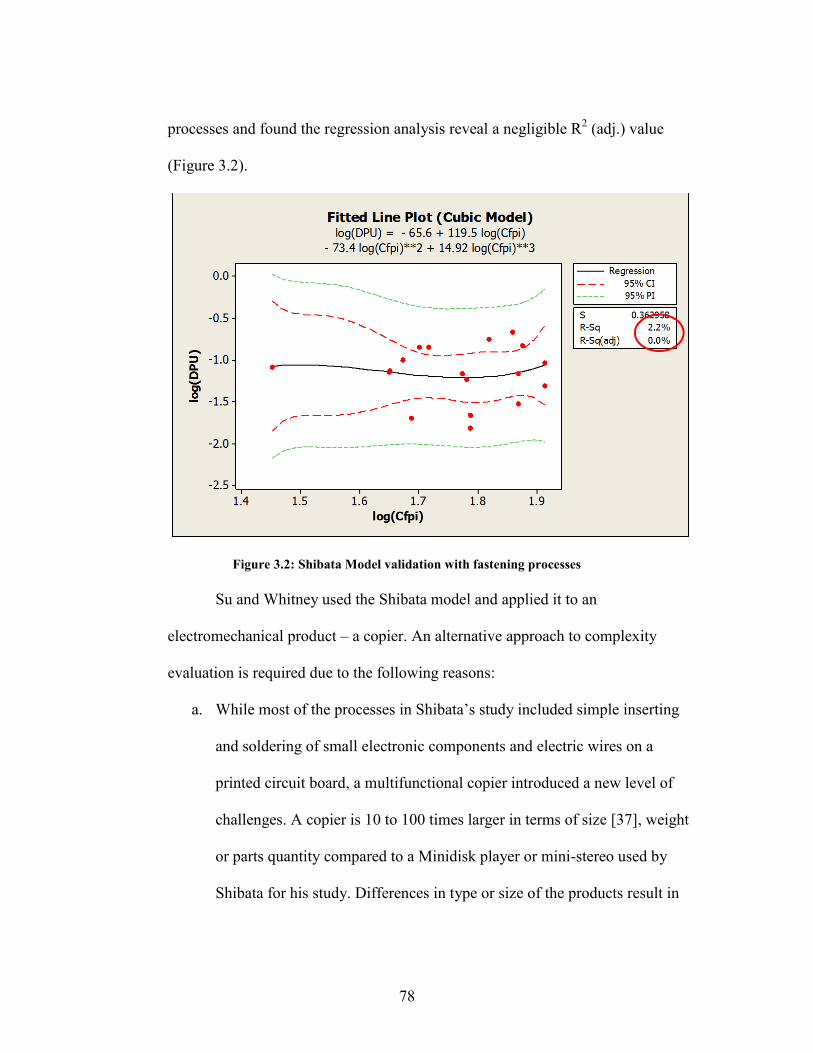
78

processes and found the regression analysis reveal a negligible R2 (adj.) value

(Figure 3.2).

Figure 3.2: Shibata Model validation with fastening processes

Su and Whitney used the Shibata model and applied it to an

electromechanical product – a copier. An alternative approach to complexity

evaluation is required due to the following reasons:

a. While most of the processes in Shibata’s study included simple inserting

and soldering of small electronic components and electric wires on a

printed circuit board, a multifunctional copier introduced a new level of

challenges. A copier is 10 to 100 times larger in terms of size [37], weight

or parts quantity compared to a Minidisk player or mini-stereo used by

Shibata for his study. Differences in type or size of the products result in

79

significant differences in parts, materials, and mating methods of

components.

b. The Shibata model used a factor Di (ease of assembly of workstation i),

evaluated based on the method of design for assembly / disassembly cost-

effectiveness (DAC) developed specifically by Sony Corporation. This

was not applicable to a generalized model or specifically to the case of the

copier studied by Su et al. because the criteria used in this method to

evaluate ease of assembly were developed specifically based on electronic

products and not on mechanical or electromechanical products like

copiers.

c. Shibata used Sony standard time (SST), a commonly used time estimation

tool designed specifically for electronic component assembly, based on

field studies and statistics. This time database is also not based on standard

MTM analysis and hence prevents the model from being generalized. For

instance, in SST, the threshold assembly time t0 is 2 seconds. However, in

the case of copier assembly, the shortest adjustment action can be

completed in 0.6 seconds according to standard time studies conducted at

Fuji Xerox by Su et. al.

3) Su and Whitney Model [37]: The research conducted by Su and Whitney

focused on understanding operator induced assembly defects for a copier based on

assembly complexity factors. They attempted to overcome some of the

shortcomings of the Shibata and Hinckley models (listed above). The researchers

80

used Fuji Xerox standard time instead of Sony standard time (SST) to evaluate the

process-based assembly complexity factor in order to make it more suitable for

copier production. Secondly, as the DAC based approach used by Shibata was

developed by Sony Corporation based on small electronic products, it was found

to be inapplicable in the case of the copier. Su & Whitney used Ben-Arieh’s [55]

fuzzy expert system approach for analyzing difficulty of assembly operations

instead of using the DAC based design-complexity evaluation method used by

Shibata. The researchers selected 11 parameters as the criteria for evaluating the

design-based assembly complexity (part shape, force required, length of

components, etc.). In order to obtain an integrated index, the weights of 11 criteria

were allocated using the analytic hierarchy process (AHP) [56]. This approach is

not suitable for a generalized complexity model for the following reasons:

a. AHP has the advantage of permitting a hierarchical structure of the

criteria, which provides users with a method to prioritize them based on

assigned weights. One of the known issues with AHP is that a different

structure may lead to a different ranking. Several authors [57, 58] have

observed that criteria with a large number of sub-criteria tend to receive

more weight than when they are less details.

b. Second reason is that this model also uses a specific time standard – Fuji

standard time. It would be beneficial to develop a model based on standard

Methods-Time Measurement (MTM) analysis in order to make its

applicability across several product types.

81

c. Based on the proposed model, for example, if a fixture is implemented to

resolve an issue that is repetitive in nature, it could potentially add a few

steps to the task. Additional steps would increase the process-complexity

factor, which would result in a higher predicted failure rate. On the

contrary, in reality, such fixtures reduce variation by improving

repeatability of part location along with the stability of the component

during the assembly process and generally reduce the defect rate. This

shows that calculating process-complexity simply based on the number of

tasks and task time is not adequate. Time variation should also be

considered in complexity calculation.

3.2.1. Summary

In summary, in order to analyze the impact of manufacturing complexity on

product quality in mixed-model assembly systems, a comprehensive approach needs to be

taken to characterize and measure manufacturing complexity. To do so, one has to take

into consideration product design characteristics, process characteristics, and finally

human factors such as task ergonomics, operator training, and experience. Detailed

analysis of assembly defects at a major automotive assembly plant has revealed that

fastening of critical components using threaded fasteners is the number one driver of

assembly defects and the top 28% of all in-process assembly defects can be attributed to a

single type of controlled fastening process. Therefore, in order to study Manufacturing

Complexity and its effect on Product Quality, first we define complexity, then develop a

generalized model, use the controlled fastening process as a pilot process to validate the

82

model, and finally we show four case studies from real-world mixed-model automotive

assembly.

3.3. Research Questions (RQ)

In order to validate the hypothesis that manufacturing complexity can reliably

predict product quality in mixed-model automotive assembly, the following research

questions need to be answered:

3.3.1. Research Question 1

How is manufacturing complexity defined in the general context of assembly

operations (Figure 3.3)?

Task 1-A:

Approach: Conduct literature review specifically focused on complexity across

various domains and identify the sources of complexity applicable to assembly

operations in mixed-model assembly system. Conduct a Process Failure Modes and

Effects Analysis (PFMEA) to determine various sources of defects for a generalized

assembly process.

Outputs: Ontology of manufacturing complexity related to the general assembly

process and the corresponding ways to measure each source.

Task 1-B:

Approach: Apply the Hinckley, Shibata, and Su & Whitney Models to the controlled

fastening process to verify the validity of existing models and learn from the gaps

observed.

83

Outputs: Data driven understanding of the gaps in currently published research and a

need to determine a new approach to defining and modeling manufacturing

complexity, to ensure applicability across a wider array of general assembly

operations.

Task 1-C:

Approach: Develop a generalized model for assembly complexity based on the key

inputs identified in Task 1-A. Apply the model to controlled fastening processes in

real-world automotive assembly plant and determine whether the generalized model

captures key variables observed in the fastening process.

Output: Applicability of comprehensive generalized manufacturing complexity

modeling approach based on literature review and hands-on understanding of the

assembly variables to the mixed-model assembly domain.

84

Figure 3.3: Flow of research tasks (RQ 1)

3.3.2. Research Question 2

How is product quality defined for assembly of components in mixed-model

automotive assembly? What is the effect of manufacturing complexity on product

quality (Figure 3.4)?

Task 2-A:

Approach: Define important aspects of quality affected by complexity. Identify

metrics to measure the effect on quality.

Output: Process Failure Mode and Effects Analysis (PFMEA) for controlled

fastening process. Comparison with generalized PFMEA & complexity model to

85

identify any additional inputs related to the fastening process that were not captured

by the generalized model.

Task 2-B:

Approach: Collect and organize the defects data for the last 12 months for four

mixed-model assembly lines. Using the historical quality data, identify the processes

that had the greatest impact and lowest impact on quality for the four assembly lines,

and collect input data to compute complexity metric.

Output: Controlled fastening processes and takts with the best and worst quality will

be highlighted for detailed analysis of each complexity driving input.

Task 2-C:

Approach: Using this information, conduct regression analysis with each source of

manufacturing complexity as input and product quality as output to determine the

effect of manufacturing complexity on product quality for 12 months of historical

data from one automotive assembly plant.

Output: A comprehensive model based on regression analysis that shows the

relationship between manufacturing complexity and product quality for a controlled

fastening process used in automotive assembly. Propose rules, constraints, and

guidelines for product design, process selection and ergonomics that would reduce or

eliminate the quality defects for the takts that were analyzed.

Assessment: Apply the model to predict the quality of 20 processes in an

independent automotive assembly plant. Compare the predicted values with actual

results that were documented from historical data. Within limitations of technical

86

feasibility and plant approval, some of the proposed changes may be tried out on the

assembly line for a limited period to evaluate the improvement in quality or identify

the shortfalls of the predictive model.

Figure 3.4: Flow of research tasks (RQ 1 and 2)

3.3.3. Research Question 3

Several quality defect prevention methods are usually employed in practice.

How can these classes of defect prevention methods be incorporated to lower

complexity and minimize DPMO (Figure 3.5)?

Task 3-A:

Approach: Based on literature review, classify error-proofing systems generally used

in large automotive assembly plants.

Output: A comprehensive understanding of the classes of mistake-proofing devices

actually used in the automotive industry.

Task 3-B:

87

Approach: Incorporate mistake-proofing devices in the complexity model to enable

prediction of Defects Per Million Opportunities (DPMO) based on the application of

those devices.

Output: An enhanced model of manufacturing complexity and product quality that

includes quality defect prevention classes as inputs (e.g. active / passive information

systems). A data driven understanding of the defect prevention methods and their

impact on product quality.

Task 3-C:

Approach: Use the revised model to predict the effect of using these classes of

mistake-proofing or assembly aid devices on specific processes, historically known to

exhibit a higher defect rate. Practically implement these defect prevention methods

and monitor the actual change in defect rate and compare it with that predicted by the

model to assess the ability of the model to predict product quality as a function of

manufacturing complexity.

Output: A case-study based data driven assessment of the validity of the predictive

model and an assessment of the ability of classes of mistake-proofing devices to

lower complexity and DPMO.

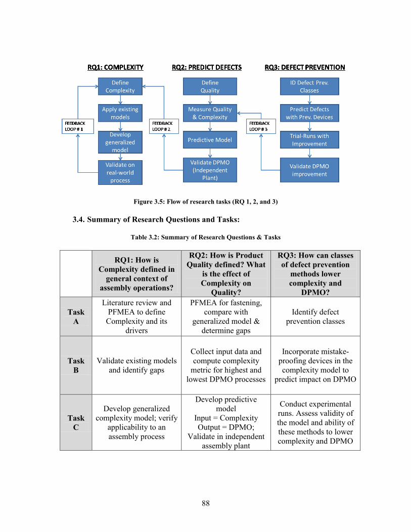
88

Figure 3.5: Flow of research tasks (RQ 1, 2, and 3)

3.4. Summary of Research Questions and Tasks:

Table 3.2: Summary of Research Questions & Tasks

RQ1: How is

Complexity defined in

general context of

assembly operations?

RQ2: How is Product

Quality defined? What

is the effect of

Complexity on

Quality?

RQ3: How can classes

of defect prevention

methods lower

complexity and

DPMO?

Task

A

Literature review and

PFMEA to define

Complexity and its

drivers

PFMEA for fastening,

compare with

generalized model &

determine gaps

Identify defect

prevention classes

Task

B

Validate existing models

and identify gaps

Collect input data and

compute complexity

metric for highest and

lowest DPMO processes

Incorporate mistake-

proofing devices in the

complexity model to

predict impact on DPMO

Task

C

Develop generalized

complexity model; verify

applicability to an

assembly process

Develop predictive

model

Input = Complexity

Output = DPMO;

Validate in independent

assembly plant

Conduct experimental

runs. Assess validity of

the model and ability of

these methods to lower

complexity and DPMO

89

CHAPTER 4

4. GENERALIZED COMPLEXITY MODEL FOR MANUFACTURING

4.1. Complexity Measurement

Based on extensive literature review and the gaps in currently published work, a

comprehensive generalized complexity model has been proposed in this research. The

sources of complexity are determined based on the following:

a) Literature review

i. Design factors [50-52, 59, 60]

ii. Process factors [5, 24, 37, 38, 47, 60-64]

iii. Human-factors [25, 37, 39, 43, 44, 60, 65-68]

b) Lessons learned from the our involvement in constraints mapping related to

assembly line balancing at a major US assembly plant [8, 69]

c) Technical input from fastening process experts at the automotive assembly

plant where this study was carried out [62]

d) Heuristic input from operators who work in mixed-model automotive

assembly

All sources of complexity are then tested for statistical significance to quantify the

ability of each input parameter (and its interaction) to account for the variation in the

resultant variable (details in Chapter 5).

Figure 4.1 shows an overview of the Product Realization Process. The scope of

this research work is limited to Product Design and Manufacturing elements of this entire

process.

90

Figure 4.1: Product Realization Process

Based on the literature review on Design for Manufacturing (DFM), process

factors, human-factors engineering (references noted in section 4.1), and complexity [5,

14-16, 38, 47], we take a holistic view in defining complexity. We re-define

manufacturing complexity as a measure of variability introduced by design factors,

process factors, and human factors that can impact functional requirements. In our

research, the functional requirements have been limited to product quality.

Figure 4.2: Key drivers of Manufacturing Complexity

4.1.1. Design Factors

Product Design is an important input variable that can impact manufacturing

complexity in a product. Using Design for Manufacturing (DFM) principles [51, 70], we

determine the input variables that can introduce manufacturing complexity. Design for

Manufacturing / Manufacturability (DFM) is a philosophy and a mind-set in which

91

manufacturing input is used at the earliest stages of design in order to design parts and

products that can be produced more easily and more economically. Tooling costs,

processing costs, assembly time, ergonomics, resulting product quality, and worker safety

are examples of some of the objectives that are considered during the DFM driven design

process [70].

The DFM process includes the following steps:

a. Determine the product characteristics

i. Functional requirements and expected life

b. Conduct Product Function Analysis

i. Design quality into the product (mistake-proofing)

ii. Reduce the number of parts

c. Design for manufacturability and usability

i. Determine materials and methods based on life expectancy

ii. Define locating surfaces and eliminate need for special fixtures

d. Define assembly process using Design for Assembly methodology

Design for Assembly (DFA) found its beginnings in the late 1970s. Manufacturers

realized that their designs were not suitable for automated assembly, and even very

difficult for manual assembly. This became an important point as volumes and variety

began increasing. Following is an example that lists a series of steps that show the

manufacturing process and the impact of DFA:

1) Purchase raw-material

2) Incoming inspection

92

3) Place material in an inventory holding location

4) Present parts to the operator or automated equipment for assembly

5) An operator picks up the part, orients it, guides it into place into a fixture

6) An operator picks up a fastener, orients it, and assembles it to the part

7) An operator picks up a tool, orients the tool, and drives the fastener

8) Final part is inspected for cross-threaded fastener, alignment etc.

Integrating assembly features into the design of the components can help eliminate

fastening components or minimize the number required. This approach would eliminate

steps 6 and 7. Perhaps, step 8 could also be eliminated or greatly simplified. This is the

basic principle of Design for Assembly (DFA). A design that is easier to assemble, is

cheaper to assemble and should encounter fewer defects. Simplifying the design is

therefore the core principle of DFA.

While using the Boothroyd and Dewhurst process [51], the following questions

have to be asked:

1) Does the part move relative to all the other parts in the assembly? Only large motions

need to be considered valid. Small movements, deflections etc. can be ignored.

2) Must this part be made of a different material from other parts in the assembly? Must

this part be isolated from other parts in the assembly? Only fundamental reasons

concerned with material properties are acceptable.

3) Must this part be separate from other parts of the assembly in order to make

assembly, disassembly or maintenance possible?

93

If the answer to any of these is No, then the part in question is a good candidate for

elimination or combination. In our research, we consider number of components being

assembled as a design complexity driver.

Figure 4.3: Design for assembly (Press fit vs. Integral shaft)

In Figure 4.3, there is a wheel pressed onto a shaft and an alternative design that

has an integral shaft. There may be cost considerations in such a design decision but it

shows how an assembly step can be completely eliminated. It is well known that threaded

fasteners are penalizing in terms of assembly. They require more time than most other

types of parts in assembly. Generally, designers recommend using snap fits for molded

plastic parts and bend-over tabs in sheet metal parts instead of threaded fasteners

wherever the functional requirements permit it. Wherever threaded fasteners must be

used, it is recommended to integrate as many other joint accessories to be integrated in

the interest of time (e.g. bolt, nut, washer, lock washer etc.). In several cases, designers

use self-locking features in the fastener to eliminate the lock washer.

Based on literature review (section 4.1), technical input from process experts in

mixed-model automotive assembly, findings from research project at an automotive

assembly plant [8, 69], and heuristic input from experienced operators, we categorize the

94

design driven complexity factors into four major categories of input variables. These can

be used to define a design-driven complexity factor (Cd). Each category will be explained

below and specific examples will be given to help the readers understand the context of

the application and give them the ability to adapt this general model to their respective

end-product / assembly being studied.

1) Feature Design (Dfd): The process of design changes the state of information

that exists about a designed object. Features are characteristics that define the

geometry, function, and aesthetics of a component [70]. A complete design

also includes the relationships among these features in terms of physical

connection, arrangement, and configuration to make up a whole part. In the

generalized complexity model, this input category includes geometric and

functional features. Aesthetic features can be added if they have any

interaction with other features or an impact on functional requirements of the

part and final assembly in which the part is used. All the features of a

component that are available should be collected in the first iteration of the

all-inclusive model. Using statistical analysis and test for significance, if the

impact of a specific feature (variable) on the resultant functional requirement

is negligible, then it can be eliminated from further analysis. The input can be

qualitative or quantitative. We will cover a brief explanation on methods to

convert qualitative information to quantitative for mathematical analysis, in

the following section. Following is an example of a feature design that could

impact functional requirements such as number of hours of continuous work

95

possible using a powertool. The handle may have a textured soft-grip material

to aid ergonomics or it may have a solid handle without the soft-grip (Figure

4.4).

Figure 4.4: DeWalt Tools without (L) & with (R) black soft-grip handle

2) Assembly Design (Dad): The assembly process generally consists of two

distinct operations: handling followed by insertion. Both these processes can

be done either manually or automatically. In order to make the assembly

process easier (which translates to reduced cost), Boothroyd [51] suggests

three key guidelines – reduce the part count, reduce the manual handling time,

and facilitate automatic handling of components. Assembly design impacts all

three of these goals and therefore impacts manufacturing complexity. Part

count can be reduced directly by achieving functional requirements with

innovative designs and thereby eliminating components or by integrating

multiple components into a larger single part by design. Manual handling time

can be reduced by avoiding nesting of components (springs) because tangled

components are difficult to grasp and manipulate with one hand. To facilitate

ease of handling, parts should be designed with symmetry in mind. Parts that

96

do not require end-to-end orientation prior to insertion are easier to handle.

Similarly, parts that have rotational symmetry take less time to orient than

ones that have a flat feature (D-shape) because the latter would require

alignment with another mating surface. Such end-to-end symmetry and

rotational symmetry can also facilitate handling in an automated handling

(bowl style component feeder). In our generalized complexity model, the

input variables under this category can be a quantitative or qualitative that

have been converted to a quantitative variable for mathematical modeling. For

example, joint design variables such as clamp load or percentage visibility of

a fastener would fall under the Assembly Design category.

3) Component Accessibility (Dac): This input variable helps us capture the

complexity introduced due to lack of direct access to the assembly area or

components being assembled. We have included this variable in the study

based on heuristic input from several experienced operators. Qualitative

(subjective) measure of accessibility should be converted into a quantitative

one based on the clear understanding of the components and the primary

reason for lack of accessibility. In the case of the fastening case study, if

multiple layers of components are between the feature to be accessed by the

associate’s hand-tool or an assembly device, then the number of layers of

components can represent a quantifiable measure for component accessibility

(Figure 4.5).

97

Figure 4.5: Layers of interference between tool and component

4) Material characteristics (Dmc): When selecting a material, the primary

concern of engineers is to ensure that the material properties are consistent

with the operating conditions of the component. The various requirements of

each component including life expectations and operating environment are

first estimated or determined. These may include mechanical characteristics

(strength, resistance to fracture, rigidity, or the ability to withstand vibrations),

physical characteristics (weight, electrical conductivity, or appearance), and

service requirements (ability operate under extreme temperature or resist

corrosion). The selection of the appropriate engineering material is often

based on the tabulated or recorded results of standardized tests [24]. A certain

property that may be required due to the function of the part can introduce

complexity in the assembly process due to other inherent properties. In

automobiles, light weight material is used wherever possible without

compromising on strength to achieve higher fuel efficiency. In the case of

fastening processes, aluminum brackets used to assemble larger parts to the

98

vehicle, introduce complexity because aluminum bends easily due to its

ductility. The dynamic change in joint gap during the fastening process can

introduce defects. Therefore, on one hand, while a certain material property is

required, it can introduce complexity in assembly that can impact an output of

interest (product quality). In the generalized complexity model, we include

quantitative material properties as input variables.

4.1.2. Mathematical formulation

In summary, four key input variables have been highlighted as contributors to

Design Complexity. If there are additional variables within each of these categories or a

new category is required for a unique process that does not fit this general model,

additional variables can be defined using the same principle. Design Complexity Factor

Cd can be mathematically expressed as follows:

1 2 3 4d fd ad ac mcC D D D D (2.20)

1..

where,

Design complexity factor

Empirical constants

Feature design variable

Assembly design variable

Component accesibility variable

Material characteristics variable

d

n

fd

ad

ac

mc

C

D

D

D

D

Figure 4.6 shows a block diagram of the four key input variables that contribute to design

complexity.

99

Figure 4.6: Input variables for design driven complexity

4.1.3. Process Factors

The goal of a process engineer is to design, develop, and implement a process that

can manufacture components that meet design specifications consistently in a cost-

effective manner. All manufacturing process display some level of variability, referred to

as inherent capability. The variability may have assignable causes such as operator errors,

defective materials, or progressive wear in the tools during machining. That variability to

which no cause can be assigned and which cannot be eliminated is inherent in the

process. Sources of inherent variability include variation in material properties, vibration

or chatter caused by tool wear, and operator variability. Therefore, process factors play a

very important role in the manufacturing complexity model. In this research, we define

five major categories of input variables that can be used to define a process-driven

complexity factor (Cp). Each category will be explained below and specific examples will

be given to help the readers understand the context of the application and give them the

100

ability to adapt this general model to their respective end-product / assembly being

studied:

1) Tooling / Fixture design (Ptf): The process engineer designs tooling and

fixtures to hold the workpiece securely and present the workpiece to the

machining tool or to the operator to enable processing in an efficient manner

while meeting dimensional specification and cycle (takt) time. The design of

the fixture can introduce dimensional variation if there is vibration, chatter or

movement in the workpiece in a way that is not part of the planned process.

This category of input variables is used to capture specific features of the

tooling or fixture design used to assemble a set of components together.

Tooling / fixture design is important especially in mass production as the

repeatability of locating and securing the components to be assembled is

critical. The tooling and fixture have to be designed in such a way that they

can tolerate the allowable component variation and the resulting tolerance

stack-up when multiple components are assembled together. This variable is

usually quantitative in nature. Examples in the context of assembly include

tool extension length, tool tip play, and process parameters.

2) Assembly Sequence (Pas): This variable is binary and reflects whether a

sequence in which components should be assembled is prescribed by the

assembly planning team or not. Set the value of the variable equal to 1 if a

sequence has been defined and set it equal to 0, if it has been left up to the

operator to decide the sequence of assembly. In general, an assembly

101

sequence is defined in cases where there may be a locating reference

associated with the first component or fastener that will be used by the

subsequent components in the assembly process. For example, there are three

bolt locations on the torsional cross-member of a Sports Utility Vehicle. One

out of three holes is the locating hole and is round in shape. The other two

holes are larger than the round hole and are usually oblong in shape to allow

for tolerance stack up of multiple components in the assembly. Hole on the

right is the locating hole (round) and the one on the left is the non-locating

hole (oblong in shape). As a first step, a fastener would have to be assembled

in the locating hole. This will help align the component with the base part.

Once aligned, fasteners can be assembled in the remaining non-locating holes.

Such requirements introduce manufacturing complexity in the assembly

operation because the process requires the operator to follow a specific

sequence of operations, without which the functional requirement of the

assembly would not be achieved. Therefore, we include it in the generalized

process model as a binary input variable.

Figure 4.7: Assembly sequence driven by locating hole

102

3) Number of tasks in the takt (Pnt): This variable captures the number of

individual tasks that have been assigned to the takt in which the assembly of

interest is being carried out. Both the Hinckley Model and Shibata Model

have shown a negative correlation between total number of assembly

operations and manufacturing complexity, when applied to semiconductor

manufacturing. A task is defined as the simplest element of work that can be

done during assembly of components. Some examples of simple tasks are as

follows:

a. Pick component from rack

b. Install component on primary sub-assembly

c. Install plug (Note: If there are several such plugs to be assembled in a

component, the installation of each plug would be considered as a

task)

4) Assembly Takt utilization (Ptu): Labor utilization is a metric that

manufacturing plants use to monitor and maximize utilization of the available

labor in each takt. The mathematical formulation of labor utilization or

assembly takt utilization is as follows:

Labor Utilization (%) =

where,

Task that belongs to a set of tasks S

=Time required per task

Number of stations ( 1,..., )

Takt time

k

j

j s

k

j

t

m c

j

t j

m k m

c

(2.21)

103

Although the objective of the production management team would be to

maximize labor utilization, manufacturing plants usually strive to achieve

between 92% - 96% average value. Especially in manufacturing systems that

are mixed-model in nature like most automotive final assembly lines, there is

a vast variety of option content (variety of different components to choose

from). Utilization value is a result of an assembly line balancing activity as

explained earlier in the background section. As the takt utilization %

increases, the process becomes less forgiving because there is little to no time

left for the operator to deviate from the tightly controlled routine. Any

deviation would introduce delay and there is no room to recover the lost time

as the assembly line operates continuously and the next product has to be

assembled in the given takt time. Therefore, we include takt utilization % as a

process input variable in the generalized complexity model.

5) Assembly Time Variation (Pvt): Variability reflects lack of repeatability in

completing a given task. If the same task is to be done over and over again, an

operator gains experience over time and slowly improves the speed at which

the same task gets done. In a mixed-model automotive assembly line, an

operator deals with a variety of tasks, one after another. The time study

analysis that helps determine how long a task takes is based on an average

value. However, often the variation in time is not taken into consideration. In

the generalized complexity model, this variable captures the time variation in

the assembly process. The variance is calculated based on a statistically

104

significant data set of actual time taken to perform the assembly or

manufacturing activity. In Shibata and Hinckley Models, work stations with

the largest number of operations or the largest time duration per task were

captured but this important input was not. From the current research, time

variation has been observed to be a statistically significant contributor and

therefore it is included in this proposed general complexity model.

4.1.4. Mathematical formulation

In summary, five key input variables have been highlighted as contributors to

process driven Complexity. Although, every effort has been made to capture the sources

of complexity in the general model, if there are additional variables within each of these

categories or a new variable is required for a unique process that does not fit this general

model, additional variables can be defined using the same principle. Process Complexity

Factor Cp can be mathematically expressed as follows:

1 2 3 4 5p tf as nt tu vtC P P P P P (2.22)

1..

where,

Process complexity factor

Empirical constants

Tooling / Fixture design variable

Assembly sequence variable

Number of tasks in takt variable

Assembly takt utilization variabl

p

n

tf

as

nt

tu

C

P

P

P

P

e

Assembly time variation variablevtP

Figure 4.8 shows a block diagram of the six key input variables that contribute to process

driven complexity.

105

Figure 4.8: Block diagram showing input variables for process driven complexity

4.1.5. Human-Factors

In cases where humans interact with systems, human-factors involves the study of

factors and development of tools that facilitate improved performance, safety, and user

satisfaction. It is important to note that some inputs may have tradeoffs. Results from

Eklund’s work at a Swedish vehicle assembly plant shows that the quality deficiencies

were three times as common for the work tasks with ergonomic problems, as compared

with other tasks [41]. This work has motivated us to determine the factors that increase

the ergonomic stress and thereby increase manufacturing complexity.

In this research, we define five major categories of input variables that can be

used to define a human-factors driven complexity factor (Ch). Each category will be

explained below and specific examples will be given wherever necessary to help the

readers understand the context of the application and give them the ability to adapt this

general model to their respective end-product / assembly being studied:

106

1) Ergonomics (Her): Ergonomics examines the interaction between the worker and

the work environment including such factors as machinery, the workstation, and

climate [71]. If the match between worker and the work environment is poor, the

worker’s ability to perform the job will be severely compromised. Over a short

period of time, this poor match may lead to fatigue and worker discomfort. If

conditions persist, physical injury, and disability may result. Ergonomics as an

input variable can be represented by a percentage value. The value reflects the

percentage of the total task time when the stress level on a certain part of the body

exceeds a threshold value. For example, if an object has to be gripped by an

operator in a given task. If the stress on the lower arms and wrists is less than 125

N for up to 30% of the total task time, then it is considered acceptable. On the

other hand, if the stress is between 190 and 285 N even for less than 5% of the

total task time, actions need to be taken to reduce that stress. Stress is classified

into multiple categories as shown in Figure 4.9.

Figure 4.9: Stress on lower arms/wrists during gripping

Similarly, there are several different ergonomic input variables that need

to be taken into consideration as individual input variables using the methodology

107

used above. Given the scope of this research, we do not focus on the scoring

methodology used in the ergonomic rating and rely on standards established at the

Original Equipment Manufacturer (OEM) where this study was conducted.

Potential users of this generalized model are advised to review the ergonomic

standards related to their respective process and use them in the model. Following

is a list of input variables tracked by the automotive assembly facility where the

current research was conducted:

a. Work height

b. Stress on neck muscles

c. Work above shoulder height

d. Mobility of trunk

e. Mobility of arms

f. Stress on arms / shoulders

g. Stress on wrists

h. Stress on fingers

i. Mobility of knee joints

j. Standing, walking, sitting

k. Handling of tools

2) Training / Experience (Htr): Argote et al. showed that large increases in

productivity are typically realized as organizations gain experience in production

[72]. These learning curves have been found in many organizations. However, the

rates at which organizations learn are different and therefore the impact on

108

productivity or quality can differ from organization to organization. Motivated by

this finding, in our research, we include training / experience in the generalized

complexity model. For an assembly process, training can be provided to operators

in various ways. A new operator can be given basic exposure to the process by

showing an audio-visual presentation that includes step by step breakdown of the

process to be followed by the operator. After an initial introduction, the operator

is typically allowed to train on an off-line training station to implement the key

points learned by observing the process in the presentation. This step is followed

by on-the-job training under expert supervision. In our generalized complexity

model, this input category can consist of a quantitative term that refers to the

physical number of hours an operator has worked on the type of process being

studied. It is important to note that the user of this generalized model should make

a data driven determination whether training / experience gained on other

“similar” processes can be taken into consideration due to the process

characteristics or not. An appropriate measure of experience should be used, such

as number of hours, number of quarters (usually 4 per shift), or number of shifts.

3) Cognitive Load (Hcl): The basic mechanisms by which humans perceive, think,

and remember are generally grouped under the label of cognition. The human

information-processing system is conveniently represented by the following three

stages at which information gets transformed:

a. Perception of information about the environment

b. Central processing or transforming that information

109

c. Responding to that information

The first and the second stages stated above are highlighted as the processes

involved in cognition and most typically represented in the study of applied

cognitive psychology [73].

In a mixed-model assembly line, one of the variants from every feature is

selected and assembled sequentially along the flow of the assembly line. For

example, say a product has two features (Fi); each feature has several variants

(e.g. Vij is the jth

variant of Fi). As depicted in Figure 4.10, V12 is chosen for F1

and V22 is chosen for F2.

Figure 4.10: Product Family Architecture and Mixed Model Assembly

Operators at every station must make correct choices from a number of

alternatives. The choices include choosing the right part, tool, fixture, and

assembly procedure for the variant. To characterize the operator performance in

110

making choices, the term operator choice complexity is defined as follows:

Choice complexity is the average uncertainty or randomness in a choice process,

which can be described by a function H in the following form:

1, 2,...,

1

( ) ( ) logM

M m m

m

H X H p p p C p p

(2.23)

Where C is a constant depending on the base of the logarithm function chosen. If

log2 is selected, C=1 and the unit of complexity is bit. The properties of the

function H are described in Ref. [20] and are suitable as a measure of choice

complexity.

In this generalized model, we simplify operator choice complexity as a

probability value. If the operator has to choose one object from a set of five

variants, the probability of picking up the correct one out of the five variants

would be 20%.

4) Work environment (Hwe): Factors such as lighting, noise, motion, thermal

conditions, and air quality contribute to the general category of Work

Environment as a variable that can impact manufacturing complexity.

a. Lighting: The amount of light energy that actually strikes the surface of

the object being seen such as a component being assembled in a factory is

described as illuminance and measured in units of lux or foot candles.

How much illuminance an object receives depends on the distance of the

object from the light source. As Figure 4.11 shows, the illuminance

declines with the square of the distance from the source. This can be

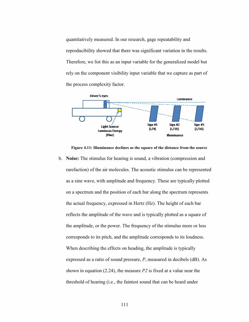
111

quantitatively measured. In our research, gage repeatability and

reproducibility showed that there was significant variation in the results.

Therefore, we list this as an input variable for the generalized model but

rely on the component visibility input variable that we capture as part of

the process complexity factor.

Figure 4.11: Illuminance declines as the square of the distance from the source

b. Noise: The stimulus for hearing is sound, a vibration (compression and

rarefaction) of the air molecules. The acoustic stimulus can be represented

as a sine wave, with amplitude and frequency. These are typically plotted

on a spectrum and the position of each bar along the spectrum represents

the actual frequency, expressed in Hertz (Hz). The height of each bar

reflects the amplitude of the wave and is typically plotted as a square of

the amplitude, or the power. The frequency of the stimulus more or less

corresponds to its pitch, and the amplitude corresponds to its loudness.

When describing the effects on heading, the amplitude is typically

expressed as a ratio of sound pressure, P, measured in decibels (dB). As

shown in equation (2.24), the measure P2 is fixed at a value near the

threshold of hearing (i.e., the faintest sound that can be heard under

112

optimal conditions). This is a pure tone of 1000 Hz at 20 micro

Newtons/square meter [68]. In this context, decibels represent the ratio of

a given sound to the threshold of hearing.

1

Sound intensity (dB) = 20log2

P

P

(2.24)

c. Motion: Stress effects of motion can result from either sustained motion

or cyclic motion. Cyclic motion is also termed as vibration in the world of

Human Factors. High frequency vibration may lead to performance

decrements or repetitive motion disorders, and low-frequency vibration is

usually a cause of motion sickness. The aversive long-term health

consequences of the high-frequency vibration are well documented in the

literature. Standard “dosage” allowances for exposure to different levels of

vibration have also been established. Health consequences of full-body

vibration have not been well documented [74]. However, such vibration

has clear and noticeable effects on many aspects of human performance

[66].

d. Thermal stress: Both excessive heat and excessive cold can produce

performance degradation and health problems. A good context for

understanding their effects can be appreciated by the representation of a

comfort zone, which defines a region in the space of temperature and

humidity and is one in which most work appears to be most productive

[75]. The temperature range is 73 deg. F to 79 deg. F in the summer and

113

68 deg. F to 75 deg. F in the winter. The zone is skewed such that less

humidity is allowed (60 percent) at the upper temperature limit of 79 deg.

F than at the lower limit of 68 deg. F (85 percent humidity allowed).

e. Air Quality: Poor air quality is often a consequence of poor ventilation in

closed working spaces like mines or ship tanks but also in environments

polluted by smog or carbon monoxide. Any of these reductions in air

quality can have relatively pronounced negative influences on perceptual,

motor, and cognitive performance of an operator [76]. This variable has

been highlighted in the generalized model for users that deal with

environments that present conditions that may compromise air quality.

Methods of quantifying this as a variable would need to be investigated

and have not been considered within the scope of the current research.

4.1.6. Mathematical formulation

In summary, four key input variables have been highlighted as contributors to

human-factors driven Complexity. Although, every effort has been made to capture the

sources of complexity in the general model, if there are additional variables within each

of these categories or a new variable is required for a unique process that does not fit this

general model, additional variables can be defined using the same principle. Human

Factors driven Complexity Factor Ch can be mathematically expressed as follows:

1 2 3 4h ef tr cl weC H H H H (2.25)

114

1..

where,

Human-factors based complexity factor

Empirical constants

Ergonomics variable

Training / Experience variable

Cognitive Load variable (Probability of choosing correct part)

h

n

ef

tr

cl

we

C

H

H

H

H

Work Environment variable

Figure 4.12: Input variables for human-factors driven complexity

4.2. Generalized Complexity Model

The generalized complexity model consists of three primary categories:

a. Design driven complexity

b. Process driven complexity

c. Human Factors driven complexity

This research aims to validate the hypothesis that manufacturing complexity

(defined by product design, assembly process, and human factors) can be represented by

a complexity metric that can be used to predict the contribution of these variables on

product quality. The generalized model correlating Product Quality (Defects per Million

115

Opportunities - DPMO) and manufacturing complexity drivers can be mathematically

described as follows:

1

0 2

3

DPMO .d p h

k

k C C C k

k

(2.26)

0

1,2,3

where,

DPMO Defects per million opportunities

Empirical process constant

Coefficient of design complexity

Coefficient of process complexity

Coefficient of human factors complexity

Empiric

d

p

h

k

C

C

C

k

al constants

In conclusion, this chapter addresses the first research question related to defining

complexity in the general context of assembly processes. In the following chapter, we use

this generalized model and apply it to a specific process that is widely used in the

automotive industry. We will then share multiple case studies related to the application of

this model to various processes in mixed-model automotive assembly and the results

achieved in each case.

116

CHAPTER FIVE

5. APPLICATION OF MODEL TO CONTROLLED FASTENING PROCESS

To validate the generalized complexity model and correlate it with product

quality, we analyzed various automotive assembly processes. Our analysis was based on

quality data gathered from one year worth of production. This eliminates any outliers

(caused by unique assignable causes) that may have contributed to a localized increase in

defect rate. Specific annual quantity is not disclosed due to confidentiality reasons. As

shown in Figure 5.1, mechanical fastening process is the largest contributor to the defect

rate of vehicles based on our study at a major OEM. Based on the data, we chose

mechanical fastening process as the pilot process to validate the generalized

manufacturing complexity model and the hypothesis that complexity can be used to

reliably predict the defect rate observed in a real-world assembly line.

Figure 5.1: Breakdown of quality defects by root cause

5.1. Overview of mechanical fastening process

117

The automotive assembly processes rely on mechanical fastening and joining to a

large extent to mount various components to the painted body. A major advantage of the

mechanical joining process is the ability to remove and mount a new component when

repair or replacement is required. Mechanical joining can also achieve an indirect way of

joining dissimilar metals, hence avoiding the galvanic corrosion effects.

A fastener is used to apply a clamp load to two or more components and maintain

it during the designed life expectancy of the assembly. The primary goal is to maintain

adequate joint clamp load that meets the design specification. The means to achieve this

goal is by tightening the fastener to a specific torque value.

Figure 5.2: Cross sectional view of a mechanical joint

The tightening process is governed by a torque-tension relationship. The

torque/tension relationship is shown in the Torque-Tension Curve [61].

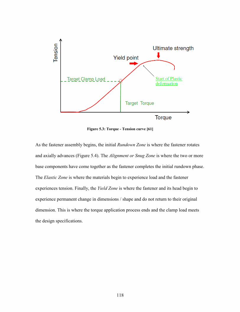
118

Figure 5.3: Torque - Tension curve [61]

As the fastener assembly begins, the initial Rundown Zone is where the fastener rotates

and axially advances (Figure 5.4). The Alignment or Snug Zone is where the two or more

base components have come together as the fastener completes the initial rundown phase.

The Elastic Zone is where the materials begin to experience load and the fastener

experiences tension. Finally, the Yield Zone is where the fastener and its head begin to

experience permanent change in dimensions / shape and do not return to their original

dimension. This is where the torque application process ends and the clamp load meets

the design specifications.

119

Figure 5.4: Tightening Zones

5.2. Thread Nomenclature

Common types of fasteners that are used in automotive applications are:

1. Bolt

2. Stud

3. Cap screw

4. Machine screw

5. Set screw

6. Nut

Basic fastening terminology is defined below [59]:

1. Major Diameter: Major diameter refers to the distance between crest to crest

for an external thread and root to root for an internal thread.

120

2. Minor Diameter: This is the diameter of an imaginary cylinder that touches

the roots of an external thread, or crests of an internal thread.

3. Internal Thread: A screw thread that is formed inside an internal diameter,

such as the hole in a nut.

4. External Thread: A screw thread that is formed on an external cylinder, such

as bolts, screws etc.

5. Pitch: The nominal distance between two adjacent thread roots or crests.

6. Thread Crest: The top part of the thread is called the Crest. For external

threads, the crest is the region of the thread that is on its outer diameter. For

internal threads, it is the region which forms the inner diameter.

7. Thread Flank: The flank is the straight side that joins the thread roots to the

crest.

8. Thread Runout: The thread root is the bottom of the thread, on external

threads the roots are usually rounded so that fatigue performance is improved.

9. Thread Length: The portion of the fastener with threads is referred to as

Threaded Length.

10. Thread Lead: The thread lead is the axial movement of the screw once

rotated one revolution.

11. Thread Root: The thread root is the bottom of the thread. On external threads

the roots are usually round so that the fatigue performance is improved.

12. Shank: The portion of a bolt that is between the head and the threaded

portion.

121

13. Bearing Stress: The surface pressure acting on a joint face directly as a result

of the force applied by the fastener.

Basic screw thread nomenclature is shown in Figure 5.5.

Figure 5.5: Thread Nomenclature [59]

ISO metric standards define the threads starting with the letter M, followed by the

nominal diameter and the thread pitch, for example, an M8 x 1.5 is an ISO thread with

diameter of 8 mm and a pitch of 1.5 mm.

An important parameter in the fastening process is the load-bearing surface area.

This controls the fastener performance during the service life of the assembly. Typically,

the average area can be defined based on an average diameter from the minor to the pitch

diameters. It is numerically shown by the following relationship (2.27):

( )16

avg p rA d d

(2.27)

122

Minor diameters (dr) and pitch diameter (dp) for ISO threads are defined in the following

equations. The nominal diameter is represented by d in the following equations:

0.6495pd d p (2.28)

1.2268rd d p (2.29)

0.6495

pd dN

(2.30)

1.299

rd dN

(2.31)

The required preload for non-permanent mechanical joints is given by:

0.75pre avg pF A (2.32)

Here, p is defined as the proof strength of the bolt and can be estimated as 85% of the

bold material yield strength. For the permanent joints, the 75% factor can be simply

changed to 90% to obtain the preload needed. And finally, the most important practical

parameter for this process is the Torque value. This equation utilizes a constant K that is

dependent on the bolt material and its size (range: 0.16 to 0.3):

preT K F d (2.33)

Where,

T = Torque

Fpre=Preload

d = nominal diameter

5.3. Controlled Mechanical Fastening

123

In the automotive industry, several safety critical and quality critical components

are assembled using electric assembly tools with intelligent controllers and associated

monitoring devices. These tools offer operator guidance in the form of clear result

feedback via on-board LEDs or audio signals. The monitoring system for each tool is part

of a larger network that associates the torque and angle information for each fastener with

the Vehicle Identification Number (VIN). This association can prove to be useful

internally to verify that all the defects on a given vehicle have been corrected before it

gets an “all-clear” to ship out from the assembly plant. These records can also prove to be

useful in the long term if a defect is found in the field by an end-user and the

manufacturing plant needs to verify that a certain component (e.g. airbag) was fastened

correctly per the engineering specifications for a certain Vehicle Identification Number.

5.3.1. Overview of equipment

The primary components in a controlled mechanical fastening system are as

follows:

a. Tool (e.g. nutrunner or screwdriver): A nutrunner or a screwdriver

is an electrical device that has a drive motor, internal bus connection

for intelligent accessories such as a barcode reader, configurable LEDs

and an optional integrated speaker for indicating via audio signals for

operator feedback. It is also designed with an ergonomic sleeve to

improve grip and comfort for the operator. Cordless drivers are also

available and they have a battery as a power source and an on-board

wireless device to communicate with the controller (Figure 5.6).

124

Figure 5.6: Atlas Copco Tools (Above: Corded, Below: Battery driven)

b. Controller & Software: With the help of onboard software, this

device provides monitoring and control of tightening operations. The

software enables a user to communicate easily with the tool controller

using a user interface. The controller also collects data continuously

throughout the tightening process.

Figure 5.7: Atlas Copco Controller unit

125

c. Display unit: The display unit shows multiple pieces of information to

aid the operator, namely, torque value, angle through which the

fastener turns beyond threshold torque, number of fasteners remaining

to complete for a given vehicle, remaining task time, and most

importantly a red or a green signal to provide a visual confirmation of

incomplete or complete assembly to the operator.

d. Electrical cords: In the case of corded electrical units, the electrical

cord is connected to the tool on one end and the controller on the

other. The cordset conducts electricity as a source of power for the tool

and it also has a network cable that allows the tool to communicate

with the controller.

Figure 5.8: Electrical cord connects the tool with the controller

e. Bits, Sockets, and Extensions: Sockets / Drivers are based on the

type of fastener being assembled (bolt, nut, hexagonal head, internal

torx-drive, external torx-drive etc.). Primary goal of the extension is to

adapt the drive type from the tool to the socket (3/8”, ½” etc.) and to

126

allow the tool to access certain assembly areas depending on the

component design. The extension also helps improve operator safety

by avoiding the tool from being too close to the workpiece which may

introduce a risk of pinching the operator’s finger between the tool and

the workpiece.

Figure 5.9: Apex Socket, Torx Drive Bit, and Extension

5.3.2. Types of fasteners

This section contains an overview of the types of fasteners and a brief overview of

the manufacturing methods for each. Following are the primary types of fasteners and

some of their variants:

i) Bolts and Screws: Even though individual bolts and screws may be

interchangeable, a bolt is intended to be used with a nut. A screw, on the other

hand, mates with preexisting threads, or in some configurations such as self-

tapping screws, a screw can make its own threads in a component. Screws and

bolts are both externally threaded fasteners that come in a variety of

head/shoulder/shank/thread combinations, and are used to join separate

127

elements, or to fasten something into place. Bolt heads are generally made

using either forging or machining. Due to economies of scale and grain flow

properties resulting from forging, it is the preferred method. Cold or hot

forging may be used depending on the formability of the fastener material.

Machining is used for very large diameters (> 1.5”) or small production runs

[63]. The disadvantage of machining is that the process cuts the grain flow,

thus resulting in planes of weakness at the critical sections such as the fillet

area. This can result in reduced tension performance resulting from fracture

planes. A generous radius should be provided under the head in order to

minimize the notch effect, without losing too much load bearing area under

the head.

ii) Bolt forms: Hexagon head bolts are available in two basic configurations:

standard hex bolts, and heavy hex bolts. Heavy hex bolts have head

dimensions that are approximately 1/8” wider than standard hex bolts

throughout the range, thereby usefully increasing the bearing surface area. The

material specification for both types is ASTM A307.

iii) Nuts: The most common shapes for nuts are square and hex. Square nuts are

more liberal in their tolerances compared to hex nuts and therefore they are

restricted to lighter-duty applications. Hex nuts come in many configurations,

in standard and heavy versions, and in thinner sizes known as jam nuts. Jam

nuts are used as locking nuts. During our research conducted at an automotive

OEM, we have come across only hex nuts and therefore those are within the

128

scope of our pilot application. For moderate temperatures and pressures,

ASTM 194 Grade 2 nuts are recommended [63].

iv) Common screws, machine screw head and thread configurations:

Hexagon head cap screws are the most commonly used screws. There are

many standardized head configurations for machine screws. There are also

many drive systems (Phillips head, slotted head, Torx, etc.). With the

exception of the hex head screws, all machine screws have round heads when

viewed from the top. Several types of head designs are available, such as,

Binding Head, Cheese Head, Flat Countersunk Head, Hex Head, Hex Washer

Head, Oval Countersunk Head, Pan Head, Round Head, Truss Head etc. In

our research study, we have come across Cheese Head screws used for lighter

duty curtain airbag assembly. For all these types, generally machine screws

are available with UNC and UNF Class 2A threads, or UNRC and UNRF

series threads.

v) Self-tapping and thread cutting screws: As the name suggests, these screws

have the ability to tap the threads in the component that they get assembled in.

Type AB point and type B point are the ones that are commonly used. Type B

thread forming tapping screw is used for sheet metal, nonferrous castings,

plywood and plastics. It is essentially a flat end Type AB screw, and the

metric version is covered by DIN 7940 and ISO 1478.

vi) Socket screws: This type of screws was developed for applications with

limited space. Their cylindrical head and internal wrenching features allow

129

their use in locations where externally wrenched fasteners would be

impractical. The two most pertinent classes, for socket head screws, are 10.9

and 12.9. The numerals used in Property Class designations refer to the

nominal ultimate tensile strength and nominal percent yield strength. For

example, a Property Class 10.9 fastener has 1000 MPa nominal strength, and a

yield of 90% of ultimate. ASTM A574M provides additional information

regarding metric, alloy steel socket head cap screws [63].

vii) Retained nuts and speed nuts: These are “clip on” internally threaded

fasteners that offer several advantages for assembly operations. Since they are,

essentially, floating nuts, they do not require drilling in the fixture being

attached, and they do not require drilling or tapping. This system of floating

alignment does not require special tools either. Retained nuts actually use a

threaded square nut mounted on a retaining clip, while speed nuts provide a

hole that accommodates a tapping nut.

5.3.3. Fastening Process Input Variables

Based on the generalized complexity model, we conducted detailed analysis of the

controlled fastening process. In addition to a review of published literature [8, 59, 63, 69,

77], we consulted with fastening experts and technicians at the automotive assembly

plant and gained hands-on assembly experience in order to identify and understand the

input variables that can impact manufacturing complexity. Following section provides the

description of each input variable.

5.3.4. Design factors driven Complexity (Cd)

130

As described in the generalized complexity model, Feature Design, Assembly

Design, Component Accessibility, and Material Characteristics are the primary categories

of input variables that impact design driven complexity. Figure 5.10 shows the input

variables for design driven complexity related to the mechanical fastening process.

Figure 5.10: Input variables - Design based mfg. complexity in Fastening

Following is a brief description of each input variable:

131

a) Fastener type: In this study we categorize fasteners into two types – Nut

and Bolt / Screw. In automotive fastening, there may be a stud that is

welded to the body and the nut is the driven component. On the other

hand, there may be a nut that is welded to the body or a component and

the bolt / screw is driven into the welded nut.

b) Fastener Head Design: In our study, we encountered four different head

designs – Hexagonal (1), Internal Torx (2), and External Torx (3). The

numbers in the parenthesis are what we use to numerically identify the

type of head design in the complexity model. The head design dictates the

type of bit or socket to be used and also has a direct effect on the tool bit /

socket slipping off during torque application, which would result in a

defect, requiring a second attempt or rework. This was added to the study

to understand whether the head design has an effect on the complexity

because hex nuts, hex bolts, and external torx are driven by a socket that

encapsulates the head completely during the torque application. On the

other hand, in the case of a fastener that does not have a hexagonal head

allows the driving bit to slip off, thereby leading to a defect.

c) Angle of Fastener: Angle of the fastener refers to the angle of the primary

axis of the fastener as viewed from the direction of torque application,

with reference to the vehicle floor.

132

Figure 5.11: Angle of fastener with ref. to the vehicle floor

d) Coating: Fastener coatings usually protect against corrosion, can improve

lubrication properties, and in some cases may be applied for appearance

reasons to match with other parts being assembled. Electroplating and

electro coating processes are used for coat application. Electrocoated

fasteners offer good uniformity of coat application but are usually

available in black. In contrast, electroplating offers good uniformity and

multiple colors using various dyes and a top coat. From the corrosion

standpoint, coated fasteners also reduce potential for galvanic corrosion in

bimetallic assemblies. In Figure 5.12, five different B-7 Stud Bolts are

shown after 2,000 hours of salt spray testing per ASTM B117, done by

MetCoat the company that produces FluoroKote. Case A is coated with

133

FluoroKote, Case B with Zinc Plating, Case C with Cadmium plating,

Case D was hot dip galvanized, and Case E was uncoated during this test.

Figure 5.12: Effect of various coatings (Source: Metcoat)

In our study, the only coating we have come across is Black Oxide.

Therefore, to convert this attribute information to the variable form, we

use 0 for no coating and 1 if coating exists.

e) Lubricant: Thread galling is a common in applications where the joint is

subjected to heavy load. During the tightening process, pressure builds up

between the contacting thread surfaces and the protective coating can get

broken down. Due to the absence of the oxide coating, the high points of

the threads are exposed, which increases friction. This can lead to enough

heat generation to fuse the nut and bolt together. Also, during tightening

process, if the torque application is continued beyond the point of galling,

the fastener head may get sheared off or the threads may get stripped.

Galling can be minimized by thread lubrication. In several applications, a

wax based coating is pre-applied to the fastener on the threads. This helps

134

reduce friction but it can dissipate over time due to heat. In our study, we

came across 25% processes that had a lubricant involved. Therefore, to

convert this attribute information to the variable form, we use 0 for no

lubricant and 1 if a lubricant exists.

f) Locking Features: Locking features are either designs in the fastener or

are added in the form of an adhesive on the threaded region. Depending on

the function of the joint and the assembly, locking features may or may

not be required. If the assembly is going to be exposed to vibration in

regular service, then locking features may be recommended to prevent the

fastener from losing clamping load.

g) Thread diameter: Major diameter refers to the distance between crest to

crest for an external thread and root to root for an internal thread. In our

research, we measured this variable for each fastener with a micrometer.

The unit of measurement was micrometer.

h) Fastener Engagement Length: As the name suggests, this refers to the

actual length along which the screw and nut are engaged and can bear the

load of the assembled joint. In our research, we measured this variable for

each fastener with a pair of vernier calipers. The unit of measurement was

micrometer.

i) Torque: Torque is the product of the magnitude of force and the

perpendicular distance from the force to the axis of rotation (i.e. the pivot

point). The SI unit of torque is Newton-meter (Nm). This value is

135

specified for every joint and was recorded in our study as a numerical

value in Newton-meter.

j) Tolerance Range: The tolerance range shows the total allowable range

that the torque can vary across. This value is also specified by the joint

designers and was recorded in our study as a numerical value in Newton-

meter.

k) Fastener Visibility: If a fastener is not clearly visible to an operator, then

it adds to the complexity of the operation and the operator would rely on

experience to guide him/her due to the lack of visibility. This situation can

occur either due to the way the joint is designed or due to poor

illumination of the workspace. In this category under the design-driven

complexity, we focus on the % visibility due to the way the joint is

designed. The value is recorded in the form of percentage and can range

from 0% in case of a completely obscured joint and 100% in the case of a

completely visible fastener, as viewed by the operator during assembly. In

our study, each joint was studied by 6 operators and an average value was

recorded as the % visibility for a given joint. The operators were trained

prior to the study to ensure that adequate repeatability and reproducibility

existed statistically in their findings.

l) Number of components assembled: This variable captures the number of

components assembled by a single fastener. As the number of components

136

to be assembled by a single fastener increases, variability associated with

the thickness of each component also increases.

m) Layers of Interference: We included this variable based on observation

of the processes. This refers to the number of surfaces related to other

components that the operator must pass the tool through in order to access

the fastener to be assembled. It is a numerical value based on CAD data

and manual observation done during the study. We have observed as many

as 2 layers of interference in our study.

n) Tensile Strength: It is the maximum tension-applied load that the fastener

can support prior to fracture. The tensile load that a fastener can withstand

is determined as follows:

2

where,

=Tensile load (N)

Tensile strength (MPa)

Tensile stress area of the fastener (mm )

t s

t

s

P S A

P

S

A

(2.34)

Tensile strength can be found for a particular bolt by referring to

Mechanical Properties table, typically provided by the fastener

manufacturer. The guide may also provide tensile stress area directly in

the form of charts. It is important to give significant consideration to the

definition of tensile stress area, As. When a standard threaded fastener fails

in pure tension, the threaded portion is usually the one that fractures as it

has the smallest cross sectional area. Therefore, usually this area is

137

calculated through an empirical formula involving the nominal diameter of

the fastener and the thread pitch. Due to confidentiality reasons associated

with the OEM where the study was conducted, we were unable to gain

access to design documents that describe the material used to manufacture

fasteners. Therefore, we do not consider Tensile Strength, Shear Strength,

and Hardness in the complexity model at this point in time. We believe

that these are important inputs and should be used in future work where

the generalized model is applied to the fastening process or other

processes; therefore we include a brief description here.

o) Shear Strength: It is defined as the maximum load that can be supported

prior to fracture, when load is applied perpendicular to the axis of the

fastener. Load occurring in one transverse plane is known as single shear.

Double shear is a condition when load is applied in two planes and the

fastener could get sheared into three pieces. When no shear strength is

given, for common carbon steels with hardness up to 40 HRC, 60% of the

ultimate tensile strength of the bolt is typically used as acceptable shear

strength.

p) Hardness: Hardness is a measure of the material’s ability to resist

abrasion and indentation. For carbon steels, Brinell and Rockwell hardness

testing can be used to estimate the tensile strength properties of the

fastener.

5.3.5. Process factors driven Complexity (Cp)

138

As shown in the generalized complexity model, Tooling & Fixture Design,

Assembly Sequence, Number of tasks in takt, Assembly Takt Utilization, and Assembly

Time Variation are the primary categories of process factors driven complexity. Figure

5.13 shows the input variables for process driven complexity related to the mechanical

fastening process.

Figure 5.13: Input variables - Process based mfg. complexity in Fastening

Following is a brief description of each input variable:

a. Tool Extension length: Primary goal of an extension is to adapt the drive

type from the tool to the socket (3/8”, ½” etc.) and to allow the tool to access

certain assembly areas depending on the component design. The extension

also helps improve operator safety by avoiding the tool from being too close

139

to the workpiece which may introduce a risk of pinching the operator’s finger

between the tool and the workpiece. The tool extension length is defined as

the total distance from the end of the output shaft of the tool to the other end

that touches the fastener. During our study, we have observed tool extensions

that range from 0.5 inches to 24 inches in length. A longer extension can

introduce a significant amount of wobble at the tip, therefore this information

is recorded in the complexity model.

Figure 5.14: Extension and Socket

b. Total Tip Play: Every tool extension introduces multiple sources of play in

the fastening system. There is some play due to the clearance between the

output side of the tool and the driven side of the extension. Similarly, there is

additional play due to the clearance between the output side of the extension

and the driven side of the socket. At both these locations, there is a pin or a

ball joint that secures the components. Longer the tool, the effective play

increases at the tip, thereby introducing a potential wobble when the fastener

is being driven.

140

Figure 5.15: Tool extension - Total Tip Play

c. Angle of extension w.r.t. fastener axis: This variable refers to the effective

angle of the extension with ref. to the axis of the fastener due to the play and

angle at which the fastener is located with reference to the vehicle.

Figure 5.16: Effective angle of extension w.r.t. fastener axis

141

A schematic view of the angle of the extension with reference to the

fastener axis is shown in Figure 5.17. This angle can be computed as

follows:

max

1 2tane

p

l

(2.35)

max

where,

Effective angle of extension w.r.t. fastener axis

Total tip play (both sides of axis)

Length of extension

e

p

l

Figure 5.17: Schematic diagram showing effective extension angle

d. Tool Trigger type: This variable helps us capture the type of tool trigger

mechanism. There are two types of mechanisms that we have observed: A

trigger that needs pulled with one finger and another one that is larger paddle

type trigger that allows the operator to pull it with four fingers. When the

operator uses this several hundred times in a given shift, that can be a variable

142

that impacts the number of trigger slip-offs. We capture this information

numerically by using the digit 1 for one finger type activation and 2 for

multiple finger paddle type activation.

Figure 5.18: Tool activation trigger: 1 finger vs. Multi-finger

e. Hand / Tool Start: This variable captures whether a fastener is hand-started

or tool-started with a low torque tool before applying higher torque with a

conventional tool, or not. Starting the fastener with a low torque (by hand or

low speed, low torque tool) significantly reduces the probability of cross-

threading the fastener when torque is applied with a conventional tool. We

capture this as a binary input – 0 for no hand-start and 1 for hand-start.

Figure 5.19: Hand-starting a fastener to prevent cross-threading

143

f. Tool Speeds (Initial and Final stages): Typically in a controlled torque

application, the tool is programmed to complete the torque application in two

stages. The tool runs at a faster initial speed (e.g. 300 RPM) during the run-

down stage (Figure 5.20) and once a designed threshold torque is achieved

(e.g. 25 Nm), the speed is dropped (e.g. 100 RPM) until the fastener reaches

the designed torque specification (e.g. 45 Nm). In our study both these speeds

have been recorded for each joining process in Rotations per Minute (RPM).

Figure 5.20: Torque-Tension evolution with time in a mechanical joint

g. Fastening Sequence: For certain component assemblies, a fastening sequence

is required or recommended. This is usually because there is a locating hole in

a component which needs to be aligned first using a fastener and then

remaining fasteners can follow. In figure, a cross member of a Sports Utility

Vehicle is shown. The hole on the far right (marked with the digit 1) is a

round hole which locates the component with reference to the body and the

remaining three holes (2a, 2b, and 2c) are oblong and these are designed to

144

allow for variation associated with tolerances of multiple components. In our

study, we capture this information as a binary variable as well. The digit 0 for

no recommended sequence and the digit 1 for joints where a specific sequence

has been recommended by process engineers.

Figure 5.21: Example showing recommended sequence of fastening

h. Number of tasks in takt: As assembly line is a flow oriented production

system where parts are assembled together to form an end product at work

stations situated along the line. A station is a location on the assembly line

where work is performed on the product. Each station may contain multiple

takts defined by some criteria (e.g. 9 work zones on a station for car

assembly). A task is the smallest, indivisible, and rational work element of the

total work content. There can be multiple tasks assigned to an operator who

works in a given takt. The process engineer’s goal is to assign as many tasks

as possible to a given takt (Figure 5.22), while ensuring that various

145

constraints such as task precedence, tooling availability, available takt time

etc. are satisfied. In this study we capture the total number of tasks that an

operator is assigned, in addition to the controlled fastening operation in a

given takt. This information was captured for each takt where the fastening

operations that were studied, took place.

Figure 5.22: Assembly line showing stations, takts, and tasks

i. Max. # of fasteners to assemble in same task: This variable captures the

total number of fasteners of the same type to be assembled by an operator to

assemble a given component. During our study, we have observed

components where up to 7 fasteners are assembled by an associate. This

repetitive task impacts manufacturing complexity and product quality in an

interestingly counter-intuitive way. The details will be discussed in the

following sections along with regression analysis.

j. Takt utilization %: Takt utilization refers to a labor utilization metric that is

generally followed by manufacturing plants to maximize the use of available

takt time (cycle time) in each takt. Mathematically, labor utilization can be

calculated as follows:

146

Labor Utilization =

where,

Task that belongs to a set of tasks

Time required per task

Number of stations (1,..., )

Takt time or Cycle time

k

j

j S

k

j

t

m c

j S

t j

m k m

c

(2.36)

In our research, we have recorded takt utilization as a % value for each takt in

which the fastening operations were carried out.

k. Avg. time per fastener (non-defective): This metric shows the average time

actually taken by operators to complete assembly of one fastener per the

required process specifications. The controlled fastening process captures the

exact duration of the process by tracking the exact time when the trigger first

gets pulled to the time when the torque and angle specifications reach their

specified target values. The average values were computed from several

thousand data points that represented processes carried out over several shifts

by various operators, and utilized a large population of components, including

fasteners. Data is captured in the form of a numerical value for each process in

milliseconds.

l. Assembly time variance: This is an important variable that has not been used

by researchers in modeling complexity, to the best of our knowledge.

Although task time has been used by several researchers as a primary driver,

we have observed that the variation in the time taken to complete the fastening

process is a significant input variable in the complexity model. Similar to the

147

method we used to capture average time per fastener, we used the same data

set, although the only difference being the inclusion of all data points

(defective and non-defective fastening cycles). Capturing those data points

that reflect the struggle that the operator had in order to meet specification, is

very important. Time variance is captured as the square of standard deviation

calculated from the large population of data points for each process.

5.3.6. Human factors driven Complexity (Ch)

As shown in the generalized complexity model, Ergonomics, Training /

Experience, Cognitive Load, and Work Environment are the primary categories of input

variables that impact human-factors driven complexity. Figure 5.23 shows the input

variables for human-factors driven complexity related to the mechanical fastening

process.

Figure 5.23: Input variables - Human-factors based mfg. complexity in Fastening

148

For this analysis, we used the ergonomic inputs that were recorded by the OEM

for each fastening task based on standard OSHA regulations that apply to the automotive

industry. Following is a brief description of each input variable and the acceptance

criteria for each variable that the OEM follows. We have used this information to

compare and contrast various fastening processes and have not considered challenging

their validity to be within the scope of this research.

a. Work height: It is defined as the height at which the operator assembles the

part with reference to the surface on which he/she is standing. This

information is recorded in terms of linear height in centimeters.

Ergonomically, work height between 85 cm and 120 cm is considered to be

acceptable. Anything below or above would need improvement (Figure 5.24).

Figure 5.24: Work Height - Acceptance criteria

b. Stress on neck: Static stress and extensive deflection is recorded as a

percentage of total time when the operator experiences it. Below 5% of total

task time is considered acceptable. Between 5% to 30% is considered as an

149

opportunity for improvement and above 30% of the total task time is

considered unacceptable.

Figure 5.25: Stress on Neck Muscles - Acceptance criteria

c. Work above shoulder height: Working above shoulder height during

fastening (e.g. working on sunroof or curtain airbag assembly from inside the

passenger cabin in a car) can be difficult for the operator and can cause

fatigue. It is important to note that the effort (load) also has to be considered

along with the % of task time that the operator conducts work above shoulder

height. For loads less than 10N, task time below 5% of total is considered

acceptable. Between 5% to 30% is considered as an opportunity for

improvement and above 30% of the total task time is considered unacceptable.

Working in a lasting static posture is unacceptable above 5% of the time.

Figure 5.26: Work above shoulder height

150

d. Mobility of trunk: Fastening tasks that involve mobility of trunk are recorded

using the following conditions:

1. Turning < 15 and/or bending 15 to < 30: Acceptable upto 30% of

total task time

2. Turning ≥ 15 and/or bending ≥ 30 to < 90: Acceptable upto 5% of

total task time

3. Bending ≥ 90 and or turning in difficult conditions: Considered

unacceptable

Figure 5.27: Mobility of trunk

e. Mobility of arms: This ergonomic variable helps us identify if the arm

movement including shoulder joint exceeds 60 cm radius during the fastening

151

operation. Less than 5% of the total task time is acceptable. If it is between

6% to 30%, it needs to be improved and greater than 30% is unacceptable.

Figure 5.28: Mobility of the arms

f. Stress on lower arms and wrists: Gripping a component or tool while

fastening can cause stress on the lower arms and wrists. If the stress on the

lower arms/wrists is less than 125 N for up to 30% of the total task time, then

it is considered acceptable. On the other hand, if the stress is between 190 and

285 N even for less than 5% of the total task time, actions need to be taken to

reduce that stress. Stress is classified into multiple categories as shown in

Figure 5.29.

Figure 5.29: Stress on lower arms / wrists - Acceptance criteria

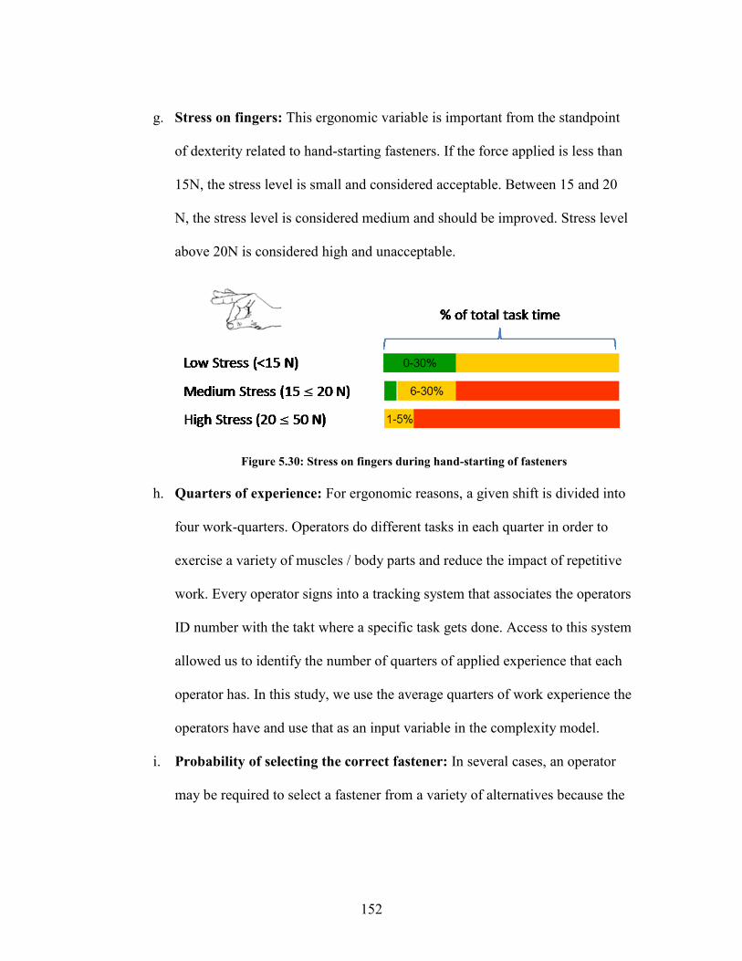
152

g. Stress on fingers: This ergonomic variable is important from the standpoint

of dexterity related to hand-starting fasteners. If the force applied is less than

15N, the stress level is small and considered acceptable. Between 15 and 20

N, the stress level is considered medium and should be improved. Stress level

above 20N is considered high and unacceptable.

Figure 5.30: Stress on fingers during hand-starting of fasteners

h. Quarters of experience: For ergonomic reasons, a given shift is divided into

four work-quarters. Operators do different tasks in each quarter in order to

exercise a variety of muscles / body parts and reduce the impact of repetitive

work. Every operator signs into a tracking system that associates the operators

ID number with the takt where a specific task gets done. Access to this system

allowed us to identify the number of quarters of applied experience that each

operator has. In this study, we use the average quarters of work experience the

operators have and use that as an input variable in the complexity model.

i. Probability of selecting the correct fastener: In several cases, an operator

may be required to select a fastener from a variety of alternatives because the

153

remaining fasteners are used at that takt for some other fastening operation.

Mathematically, this probability can be expressed as follows:

1

where,

Probability of selecting the correct fastener

Number of available alternative fasteners are the same takt

f

f

f

f

pn

p

n

(2.37)

j. Work environment: Under this category, we consider Noise, Lighting,

Humidity, and Temperature. As noise, humidity, and temperature were quite

similar in the manufacturing facility where the processes were studied, we do

not consider them in the complexity model specifically for this pilot study.

We consider lighting and as explained in Chapter 4, the term illumination

characterizes the lighting quality of a given working environment. How much

illuminance an object receives depends on the distance of the object from the

light source. An alternative method is based on analysis of photographs to get

a relatively subjective input from the operators and convert it to a numerical

value on a relative scale. Pictures of the assembly process to be studied can be

taken consistently with the same camera while maintaining the same average

distance between the assembly and the operator’s eyes. These photographs

can be studied by various operators who are trained to work on similar

assemblies and a score can be assigned on a pre-determined scale to compare

the level of illumination for each assembly process being studied.

5.4. Application of proposed model to pilot process

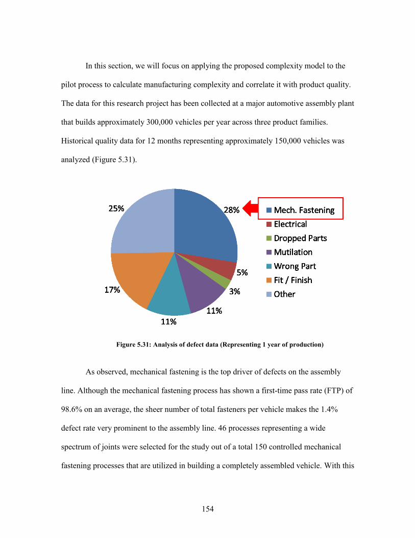
154

In this section, we will focus on applying the proposed complexity model to the

pilot process to calculate manufacturing complexity and correlate it with product quality.

The data for this research project has been collected at a major automotive assembly plant

that builds approximately 300,000 vehicles per year across three product families.

Historical quality data for 12 months representing approximately 150,000 vehicles was

analyzed (Figure 5.31).

Figure 5.31: Analysis of defect data (Representing 1 year of production)

As observed, mechanical fastening is the top driver of defects on the assembly

line. Although the mechanical fastening process has shown a first-time pass rate (FTP) of

98.6% on an average, the sheer number of total fasteners per vehicle makes the 1.4%

defect rate very prominent to the assembly line. 46 processes representing a wide

spectrum of joints were selected for the study out of a total 150 controlled mechanical

fastening processes that are utilized in building a completely assembled vehicle. With this

155

data, we develop a regression based predictive model to predict defects and validate the

model in an independent automotive assembly plant.

5.4.1. Quality Measurement

There are four key fastening process control strategies to the best of our

knowledge. Table 5.1 shows the key characteristics and the potential variation that can be

expected from each strategy.

Table 5.1: Fastening Process Control Strategies

In the processes we studied, Torque and Angle Control strategies were being

used. The closed loop control and monitoring process provides immediate feedback to the

associate whether or not the fastener (joint) has met specified torque and angle

requirements through LEDs that are mounted on the tool and also on another visual

display that is connected to the tool and controller. The controller also records torque and

angle values dynamically for each fastener and stores it for offline analysis. Figure 5.32

shows a plot with torque (N.m.) along the Y-axis and angle (deg.) along the X-axis. The

156

red line shows the dynamic torque and angle values as the fastening operation progresses.

The black dot at the intersection of 4 N.m. and a few degrees past 1,000 along the X-axis

refers to a threshold torque. This is set up by the process engineer and the tool starts

monitoring angle beyond that point until the final torque and angle specifications are

reached. The secondary X-axis shown in red font reflects the angle value starting at 0

degrees, once the threshold value is reached.

Figure 5.32: An example of a defective fastening operation (torque-angle plot)

The green box shows the allowable tolerance window for torque and angle. In this

case, the torque value crossed 4 N.m. but the fastener was unable to gain more torque and

eventually dropped off as shown by the red line. This is typically associated with a large

joint gap that the fastener is unable to close during the operation. Such a fastening

process would be considered as defective. The tool would register it and that defect stays

associated with the vehicle until it gets cleared manually by a re-worker on the assembly

line. The vehicle cannot get shipped unless all defects are cleared from the system. The

157

primary goal of process and quality engineers is to understand the root cause of such

failures and systematically implement mistake-proofing systems to prevent them from

recurring.

The quality defect rate can be computed as follows:

6# of defectsDPMO = 10

# of opportunities

where,

DPMO = Defects per million opportunities

(2.38)

In this equation, the number of opportunities is defined as the total number of attempts

(successful and unsuccessful) to assemble the fastener. For example, if on a given vehicle

to be assembled, an associate has to assemble 9 fasteners. If the operator comes across

one failure and has to make an extra attempt to complete the 9 assemblies, the total

number of opportunities that the operator had = 9 + 1 = 10.

61DPMO = 10 100,000

(9+1)

where,

DPMO = Defects per million opportunities

(2.39)

In a similar manner, 12-months of historical data was collected for all the processes that

were studied.

5.4.2. Identification of significant input factors

A total of 36 input variables were recorded for 40 fastening process along with the

respective Defects Per Million Opportunities (DPMO) for each process. Statistical

analysis was conducted using Minitab. For regression analysis, the response variable in

158

our study is DPMO and predictor variables are the 36 input variables that represent

design, process and human factors driven complexity.

Analysis of variance (ANOVA) gives p-values for each input variable (Figure

5.33). P-value determines the appropriateness of rejecting the null hypothesis in a

hypothesis test. The p-value is the probability of obtaining a test statistic that is at least as

extreme as the calculated value if the null hypothesis is true. In our study, we use the

standard alpha level of 0.05. If the p-value of a test statistic is less than the alpha, we

reject the null hypothesis. The null hypothesis in this regression study is that the input

variable does not have a significant effect on the response variable (DPMO), which

means the coefficient for that variable will equal zero in the regression equation. If the p-

value is less than 0.05, we can statistically conclude that the variable has a significant

effect on the response variable and the coefficient is significantly different from zero.

159

403020100

0.8

0.7

0.6

0.5

0.4

0.3

0.2

0.1

0.0

Input Variables (Sorted in ascending order of p-value)

p-v

alu

e

0.05

Scatter plot showing distribution of p-values of Input Variables

Figure 5.33: P-value distribution for 36 input variables (Alpha value 0.05)

Following table shows the reference number used in the plot, complexity factor of each

input variable, names of input variables, and the corresponding p-value.

Table 5.2: Input variables and the corresponding p-value (ascending order)

160

Following is a brief explanation and plots showing relationships of those individual input

variables that have shown a R2 (adj.) value of greater than 5% with Defects Per Million

Opportunities (DPMO) as a resultant variable:

Order Factor Input Variable p-value

1 C d No. of components to be assembled 0.000

2 C d Thread diameter (OD) 0.000

3 C h Probability of choosing correct fastener 0.000

4 C p Max. # of fasteners in same task 0.000

5 C d Fastener head design 0.000

6 C h Stress on neck 0.000

7 C d Locking features 0.000

8 C p Assembly Time Variance 0.000

9 C p Tool speed (final stage) 0.000

10 C d Fastener engagement length 0.001

11 C d Fastener type 0.001

12 C p Takt utilization 0.002

13 C d Lubricant 0.002

14 C h Work above shoulder height 0.003

15 C d Fastener visibility 0.006

16 C p Tool speed (initial stage) 0.010

17 C h Stresses on fingers 0.012

18 C p Avg. assly. time per fastener 0.039

19 C p Hand / Tool start 0.052

20 C h Stresses on lower arms 0.091

21 C p Fastening sequence 0.120

22 C p Effective Tip Play 0.167

23 C d Coating 0.181

24 C h Mobility of arms 0.206

25 C p Tool trigger type 0.207

26 C d Layers of interference 0.208

27 C d Tolerance range 0.264

28 C d Angle of fastener 0.284

29 C p Angle of extension w.r.t. fastener 0.285

30 C h Work height 0.286

31 C p No. of tasks in takt 0.319

32 C p Total tip play 0.393

33 C d Torque 0.458

34 C h Mobility of trunk 0.722

35 C h Stresses on arms 0.750

36 C p Tool extension length 0.759

161

a) Probability of choosing the correct fastener: A fitted line plot (Figure 5.34)

shows that as the probability of choosing the correct fastener increases, the

potential for defects goes down, as intuitively expected. R2 (adj.) value was

11.5%. In the data set, we encountered two processes with the least probability of

correct choice (33.3%), where the associate had three fasteners with

interchangeable thread size and design. An incorrect choice would result in a

torque defect because the process specifications would fall outside specifications.

Several more processes had a 50% probability as shown in the plot and most

stations had only one choice of fastener which resulted in 100% probability.

10090807060504030

100000

80000

60000

40000

20000

0

Prob. of choosing correct fast.

Actu

al

DP

MO

S 18526.8

R-Sq 13.1%

R-Sq(adj) 11.5%

Regression

95% CI

95% PI

Fitted Line PlotActual DPMO = 59289 - 341.3 Prob. of choosing correct fast.

Figure 5.34: Probability of choosing the correct fastener vs. DPMO

b) Assembly time variance: Assembly time variance is an input variable that has

not been highlighted before by Shibata [38] and Hinckley [47], who developed

162

complexity models based on task time and number of operations. In our research,

we calculated the standard deviation of time taken to assemble a fastener that

meets specifications. In this calculation, we have excluded the data points for

those fasteners that were linked to defects because clearly the processes that have

more defects would have shown a correlation of the time variance vs. DPMO.

From the analysis, we found that a quadratic fitted line plot shows a low R2 (adj.)

value but still significant compared to the < 1.6% R2 (adj.) value that we observed

with time and number of operations (Figure 5.35).

180016001400120010008006004002000

125000

100000

75000

50000

25000

0

Assly. Time (SD)

Actu

al

DP

MO

S 19046.4

R-Sq 9.9%

R-Sq(adj) 6.5%

Regression

95% CI

95% PI

Fitted Line PlotActual DPMO = 41968 - 54.33 Assly. Time (SD)

+ 0.04383 Assly. Time (SD)**2

Figure 5.35: Assembly time Std. Deviation vs. DPMO (Quadratic)

c) Fastener engagement length: A linear fitted line plot (Figure 5.36) shows that as

the engagement length increases, the potential for defects is higher. We came

across a higher concentration of joints that had less than 10 mm total engagement

163

length but there were several others with higher torque specifications that ranged

between 15 to 40 mm. We found one process where several threaded components

were stacked together and the total engagement length was 66 mm. The linear

fitted line plot shows an R2 (adj.) value of 15% and a quadratic fitted line plot

shows a R2 (adj.) value of 16.2% (Figure 5.37). As the benefit of using a quadratic

model is very small in this case, we choose to use the linear relationship in the

final regression model.

706050403020100

100000

75000

50000

25000

0

Fastener engagement length

Actu

al

DP

MO

S 18157.4

R-Sq 16.5%

R-Sq(adj) 15.0%

Regression

95% CI

95% PI

Fitted Line PlotActual DPMO = 17762 + 614.9 (Fastener engagement length)

Figure 5.36: Fastener engagement length vs. DPMO (Linear)

164

706050403020100

125000

100000

75000

50000

25000

0

Fastener Engagement Length

Actu

al

DP

MO

S 18021.5

R-Sq 19.3%

R-Sq(adj) 16.2%

Regression

95% CI

95% PI

Fitted Line PlotActual DPMO = 22352 + 6.9 (Fast. Eng. Length)

+ 12.61 (Fast. Eng. Length)**2

Figure 5.37: Fastener engagement length vs. DPMO (Quadratic)

d) Takt Utilization: As highlighted in the research motivation section, when our

research group was working on an Assembly Line Balancing project at a mixed-

model assembly plant, we observed the potential need to understand

manufacturing complexity and product quality because the way tasks are arranged

on an assembly line may bear an effect on product quality. Labor utilization is one

of the primary objectives of Assembly Line Balancing. Fitted line plots of linear,

quadratic, and cubic models show R2 (adj.) values of 6.9%, 9.3%, 11.2%

respectively (Figure 5.38). As utilization drops below 80%, the corresponding

DPMO is higher. This may be due to interaction with other variables.

165

120.0%110.0%100.0%90.0%80.0%70.0%60.0%

120000

100000

80000

60000

40000

20000

0

-20000

-40000

Utilization

Actu

al

DP

MO

S 18561.4

R-Sq 16.0%

R-Sq(adj) 11.2%

Regression

95% CI

95% PI

Fitted Line PlotActual DPMO = 1424092 - 4275515 Utilization

+ 4327086 Utilization**2 - 1449062 Utilization**3

Figure 5.38: Takt utilization vs. DPMO (Cubic model)

e) Work above shoulder height (% of task time): Our study included a wide

spectrum of mechanical fastening processes across the entire automotive

assembly plant. We intentionally looked for processes that would give us a wide

range of input variables such as work above shoulder height. In our data, we came

across only 4 processes in which operators worked for 65% of their respective

task times, above shoulder height. As shown in the fitted line plot for a linear

model, the R2 (adj.) value was found to be 10.0% (Figure 5.39). A quadratic

model marginally increases it to 11.2%. However, there was a strong

concentration of processes in which the work content above shoulder height was

limited to 20% of the task time. Therefore, the decreasing trend of DPMO as the

% of time increases may be limited to this data set alone and may not be valid

166

across the entire range of processes. Also, there may be an interaction with

another variable that explains why the DPMO drops with higher percentage of

work above shoulder height.

706050403020100

80000

60000

40000

20000

0

-20000

-40000

Work abv. Shldr. Ht. (% time)

Actu

al

DP

MO

S 18680.3

R-Sq 11.7%

R-Sq(adj) 10.0%

Regression

95% CI

95% PI

Fitted Line PlotActual DPMO = 32432 - 281.1 Work abv. Shldr. Ht. (% time)

Figure 5.39: Work above shoulder height (% of task time) vs. DPMO (Linear)

f) Tool speed (initial stage): The torque application process is divided into two

parts. The rotational speed of the tool is higher in the first part and once the

threshold torque is reached, the speed drops to a lower value. This variable tracks

the initial tool speed. As shown in the fitted line plot (Figure 5.40) using a

quadratic model, the R2 value is 8.3% and except for 4 processes on the low end

below 225 RPM, the general tendency is for the DPMO to be lower as the speed

increases.

167

450400350300250200150100

100000

75000

50000

25000

0

-25000

-50000

Tool speed (Initial)

Actu

al

DP

MO

S 18860.8

R-Sq 11.6%

R-Sq(adj) 8.3%

Regression

95% CI

95% PI

Fitted Line PlotActual DPMO = - 41268 + 520.9 Tool speed (Initial)

- 0.9141 Tool speed (Initial)**2

Figure 5.40: Tool Speed (Initial phase) vs. DPMO (Quadratic)

g) Average assembly time per fastener: Average assembly time is an input

variable that was highlighted by Shibata [38] and Hinckley [47], who developed

complexity models based on task time and number of operations. The general

tendency is for defect rate to drop as the time taken to assemble a fastener is

longer. This trend contradicts what was found in previous research associated

with semi-conductor assembly and audio-players. In our study, average time per

fastener was based on approximately 18,000 to 42,000 data points (fasteners) per

process. The number of data points (fasteners) varied based on the quantity used

per assembled vehicle. Using a quadratic model (Figure 5.41), the R2 value was

found to be 7.1%.

168

70006000500040003000200010000

100000

80000

60000

40000

20000

0

-20000

Time per Fastener

Actu

al

DP

MO

S 18979.9

R-Sq 10.5%

R-Sq(adj) 7.1%

Regression

95% CI

95% PI

Fitted Line PlotActual DPMO = 51720 - 12.54 Time per Fastener

+ 0.001333 Time per Fastener**2

Figure 5.41: Average time per fastener assembly vs. DPMO (Quadratic)

h) Work height: In our study, most of the processes were conducted by operators

between 100 cm to 140 cm. There were 4 processes that were conducted at 160

cm. with reference to the level at which the operators were standing. Although the

quadratic fitted line plot shows the tendency for the DPMO to drop as work height

increases beyond 140 cm, the available data may not be statistically sufficient to

draw that conclusion. This should be noted as the framework of this model is

applied to other processes in future. The R2 (adj.) value was found to be 7.5%

using a quadratic model (Figure 5.42).

169

160150140130120110100

80000

60000

40000

20000

0

-20000

-40000

Work Height

Actu

al

DP

MO

S 18943.2

R-Sq 10.8%

R-Sq(adj) 7.5%

Regression

95% CI

95% PI

Fitted Line PlotActual DPMO = - 258072 + 4712 Work Height

- 18.90 Work Height**2

Figure 5.42: Work height vs. DPMO (Quadratic)

i) Tool extension length: In our study, we were able to capture a very wide range of

tool extension lengths (5mm to > 400 mm). The general tendency of the process is

to have higher level of defects as the length increases because of the increased tip

play (wobble) associated with the inherent vibration of the output spindle that is

multiplied by the length of the extension. This causes slip-offs, a condition where

the tool jumps off the fastener head and causes an intermittent drop in torque

value or a complete shutdown of the process. The fitted line plot shows a R2 (adj.)

value of 5.3% using a quadratic model (Figure 5.43). The linear model and cubic

model generate a R2 (adj.) value of 2.3% and 6.8% respectively.

170

4003002001000

80000

60000

40000

20000

0

-20000

-40000

Ext. Length

Actu

al

DP

MO

S 19159.4

R-Sq 8.8%

R-Sq(adj) 5.3%

Regression

95% CI

95% PI

Fitted Line PlotActual DPMO = 13116 + 192.3 Ext. Length

- 0.4056 Ext. Length**2

Figure 5.43: Tool extension length vs. DPMO (Quadratic)

In summary, these individual fitted line plots show some interesting correlation

between these individual variables and product quality (DPMO). We gain a better

understanding of the process using this information and develop a predictive model,

details of which are shared in the next section.

5.4.3. Development of predictive model

Based on the statistical analysis, we know the factors that have a significant

impact on product quality measured as DPMO. We conduct regression analysis to

investigate the model the relationship between the response variable (DPMO) and the

predictors (input variables). We perform Ordinary Least Squares (OLS) regression [78].

In OLS regression, the estimated equation is calculated by determining the equation that

minimizes the sum of the squared distances between the sample’s data points and the

171

values predicted by the equation. OLS regression will provide precise, unbiased estimates

only when the following assumptions are met:

1) The regression model is linear in the coefficients. Least squares can model

curvature by transforming the variables (rather than the coefficients).

Functional form of the equation needs to be specified in order to model the

curvature. In our data, linear model was sufficient.

2) Residuals have a mean of zero. Inclusion of a constant in the model will force

the mean to equal zero.

3) All predictors are uncorrelated with the residuals.

4) Residuals are not correlated with each other (serial correlation).

5) Residuals will have a constant variance.

6) No predictor variable is perfectly correlated with another predictor variable.

7) Residuals are normally distributed.

Because OLS regression will provide the best estimates only when these

assumptions are met, it is important to test them. Common methods include examining

residual plots and using lack of fit tests.

In regression analysis, R2 (R-sq) is the coefficient of determination. It indicates

how much variation in the response variable is explained by the model. The higher the R2

value, the better the model fits the data set of predictor variables.

2

2

2

ˆSS Error1 1

SS Total

i i

i

y yR

y y

(2.40)

172

where,

observed response value

mean response

ˆ fitted response

th

i

th

i

y i

y

y i

Best Subsets regression is a method that is used to identify the subset models that

produce the highest R2 values from a full set of predictor variables [79]. It offers an

efficient way to identify models that achieve the goals with as few predictors as possible.

Minitab examines all possible subsets of the predictors, beginning with all models

containing one predictor, and then all models containing two predictors, and so on. The

two best models for each number of predictors are displayed. It also displays a Mallows’

Cp value for each predictor set. Mallows Cp is a measure of goodness-of-prediction. The

formula is as follows:

SSE

Mallows' ( 2 )MSE

p

p

m

C n p

(2.41)

where,

SSE Sum of squares error for the model

MSE Mean square error for the model with all predictors

number of observations

number of terms in the model, incl. constant

p

m

n

p

For analysis, we want to look for models where the Mallow’s Cp is small and

close to the number of predictor variables. A small Cp indicates that the model is

relatively precise (has less variance) in estimating the true regression coefficients and

predicting future responses. Models with poor predictive ability and bias have values of

Cp larger than the number of predictors.

173

Three different cases of regression based predictive models are described below.

5.4.4. Regression Model – Iteration 1 (6 variables)

We conducted analysis of statistical-significance (p-value) and regression analysis

with all the variables. Although the p-value for Work Height, Total Tip Play, Torque,

Tool Extension Length, and Fastening Sequence was greater than the 0.05 threshold

(Table 5.2), we observed an impact on the net R2 (adj.) value, therefore we included them

in the best-subsets analysis.

Table 5.3 shows a summary of top two subsets for each number of predictor

variables. A total of 16 factors have the ability to account for 77% of the variation in

DPMO. For ease of explanation, we have limited the best-subsets table to 77% (or 16

variables). Increasing the total number of variables to 24 increases the R2 (adj.) value to

93% but we will cover this in iteration # 3. In this iteration, we select the subset with 6

variables that can account for 53.1% of the DPMO variation. Although the Mallows’ Cp

is significantly higher than the number of predictor variables, we select it as a baseline

iteration that explains 50% of the DPMO variation (R2-adj. value).

174

Table 5.3: Best-Subsets Analysis

# o

f V

ariable

s

R-S

q

R-S

q(a

dj)

Ma

llow

s' C

p

S

Work

heig

ht

Str

ess o

n n

eck (

% o

f tim

e)

Work

above s

hld

r. h

t. (

% o

f tim

e)

Fa

ste

ne

r he

ad

desig

n

To

tal tip

pla

y

Fa

ste

ne

r ty

pe

Ma

x.

# o

f fa

ste

ne

rs in

ta

kt

Lockin

g

Sequence

Co

mp

on

en

t Q

ty.

Th

rea

d O

D

To

ol sp

eed

(F

ina

l)

Pro

b. of corr

ect choic

e

Assly

. T

ime (

Std

. D

ev.)

Fa

ste

ne

r en

ga

ge

men

t le

ng

th

Utiliz

atio

n

1 16.5 15.0 150.3 18,157 X

1 13.1 11.5 158.7 18,527 X

2 25.6 22.8 130.3 17,299 X X

2 24.1 21.2 134.0 17,478 X X

3 35.7 32.0 107.8 16,234 X X X

3 30.4 26.3 120.8 16,902 X X X

4 44.3 39.9 89.0 15,261 X X X X

4 41.2 36.6 96.4 15,675 X X X X

5 50.6 45.7 75.7 14,515 X X X X X

5 46.6 41.2 85.5 15,095 X X X X X

6 58.2 53.1 59.4 13,493 X X X X X X

6 56.0 50.7 64.5 13,832 X X X X X X

7 61.8 56.3 52.5 13,022 X X X X X X X

7 61.0 55.3 54.5 13,164 X X X X X X X

8 65.8 60.0 44.9 12,455 X X X X X X X X

8 64.2 58.1 48.8 12,751 X X X X X X X X

9 69.5 63.5 38.0 11,900 X X X X X X X X X

9 68.6 62.5 40.1 12,061 X X X X X X X X X

10 73.7 67.8 29.8 11,169 X X X X X X X X X X

10 71.5 65.1 35.2 11,632 X X X X X X X X X X

11 76.6 70.8 24.6 10,640 X X X X X X X X X X X

11 74.8 68.6 29.0 11,043 X X X X X X X X X X X

12 78.5 72.5 22.2 10,331 X X X X X X X X X X X X

12 77.5 71.2 24.6 10,566 X X X X X X X X X X X X

13 80.1 73.9 20.3 10,056 X X X X X X X X X X X X X

13 79.5 73.1 21.7 10,204 X X X X X X X X X X X X X

14 82.5 76.6 16.4 9,535 X X X X X X X X X X X X X X

14 81.6 75.3 18.6 9,784 X X X X X X X X X X X X X X

15 83.6 77.5 15.6 9,338 X X X X X X X X X X X X X X X

15 82.8 76.3 17.8 9,584 X X X X X X X X X X X X X X X

16 83.9 77.3 17.0 9,380 X X X X X X X X X X X X X X X X

175

Using these predictor variables, we construct a regression model. Following are

the equations for each complexity factor:

1) Design driven complexity factor (Cd):

_ _ _

_

5499.4 12197.8 1352.72

27671.7

d fd OD fd hed fd len

fd typ

C D D D

D

(2.42)

_

_

_

_

where,

Feature design - Thread Diameter (mm)

Feature design - Fastener head design (number)

Feature design - Thread engagement length (mm)

Feature design - Fastener type (nu

fd OD

fd hed

fd len

fd typ

D

D

D

D

mber)

2) Process driven complexity factor (Cp):

_

_

467.8

where,

Tooling & fixture design - Total tip play (mm)

p tf tip

tf tip

C P

P

(2.43)

3) Human-factors driven complexity factor (Ch):

_

_

362.46

where,

Cognitive load - Probability of correct choice (%)

h cl pro

cl pro

C H

H

(2.44)

4) Correlating Complexity to DPMO:

DPMO = 56600.2 + d p hC C C (2.45)

where,

DPMO = Defects per million opportunities

Design driven complexity factor

Process driven complexity factor

Human factors driven complexity factor

d

p

h

C

C

C

176

The following plots show the residual analysis based on the regression model with

6 input variables, applied to the 39 fastening processes. The normality plot shows that the

p-value is significantly smaller than the threshold alpha value of 0.05 which shows that

the residuals (Figure 5.44) are not normally distributed. Similarly, the histogram (Figure

5.45) shows a different view of the same data and shows the outlier with a large residual

value of 36,000. Clearly, this shows that although we have a model that can account for

50% of the variability in the resultant DPMO, the model needs to be improved.

400003000020000100000-10000-20000-30000

99

95

90

80

70

60

50

40

30

20

10

5

1

Residual values

Pe

rce

nt

Mean -1267

StDev 11759

N 39

AD 1.080

P-Value 0.007

Probability Plot of Residuals

Figure 5.44: Normality plot of residual values (Iteration 1)

177

32000160000-16000

16

14

12

10

8

6

4

2

0

Residuals

Fre

qu

en

cy

Histogram of Residuals

Figure 5.45: Histogram of Residuals (Iteration 1)

5.4.5. Regression Model – Iteration # 2 (16 variables)

Based on the best subsets analysis (Table 5.3), in this iteration we choose the

subset with 16 variables. The estimated R2 (adj.) value is 77% and the corresponding

Mallows Cp value is 17, which is very close to the total number of predictor variables in

this model.

Using these predictor variables, we construct a regression model. Following are

the equations for each complexity factor:

1) Design driven complexity factor (Cd):

_ _ _

_ _ _

6602.17 7808.1 14264.5

12259.4 1223.2 34466.2

d ad qty fd OD fd hed

fd loc fd len fd typ

C D D D

D D D

(2.46)

178

_

_

_

_

where,

Assembly design - Assly. Component qty. (number)

Feature design - Thread Diameter (mm)

Feature design - Fastener head design (number)

Feature design - Locking (binary

ad qty

fd OD

fd hed

fd loc

D

D

D

D

_

_

)

Feature design - Thread engagement length (mm)

Feature design - Fastener type (number)

fd len

fd typ

D

D

2) Process driven complexity factor (Cp):

_ _ _

_ _ _ 2

648.8 21047 12764.6

9.6 4335 92.14

p tf tip as seq tu utl

vt sd nt qty ad sp

C P P P

P P D

(2.47)

_

_

_

_

_

where,

Tooling & fixture design - Total tip play (mm)

Tooling & fixture design - Sequence (binary)

Assly. Takt utilization (%)

Assly. Time - Standard Deviation (ms)

N

tf tip

as seq

tu utl

vt sd

nt qty

P

P

P

P

P

_ 2

umber of fasteners in takt (number)

Tooling & fixture design - Tool speed final (RPM)tf spP

3) Human-factors driven complexity factor (Ch):

_ _ _

_

276.6 233.4 349.4

361.1

h er wkh er nec er sho

cl pro

C H H H

H

(2.48)

_

_

_

_

where,

Ergonomics - Work height (cm)

Ergonomics - Stress on neck (% of task time x 100)

Ergonomics - Work above shoulder height (% of task time x 100)

Cognitive load - Prob

er wkh

er nec

er sho

cl pro

H

H

H

H

ability of correct choice (%)

4) Correlating Complexity to DPMO:

179

DPMO = 33381.1 + d p hC C C (2.49)

where,

DPMO = Defects per million opportunities

Design driven complexity factor

Process driven complexity factor

Human factors driven complexity factor

d

p

h

C

C

C

20000100000-10000-20000

99

95

90

80

70

60

50

40

30

20

10

5

1

Residuals

Pe

rce

nt

Mean -616.8

StDev 7926

N 39

AD 0.367

P-Value 0.416

Probability Plot of ResidualsNormal

Figure 5.46: Normality plot of Residuals (Iteration 2)

180

12000800040000-4000-8000-12000-16000

9

8

7

6

5

4

3

2

1

0

Residuals

Fre

qu

en

cy

Histogram of Residuals

Figure 5.47: Histogram of Residuals (Iteration 2)

5.4.6. Regression Model - Iteration # 3 (24 variables)

Based on the analysis of statistical significance (p-value) and multiple regression

analysis iterations, it was found that the following input variables consistently have a

strong impact on the resultant variable (DPMO):

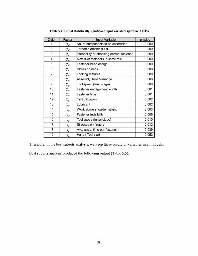
181

Table 5.4: List of statistically significant input variables (p-value < 0.05)

Therefore, in the best subsets analysis, we keep these predictor variables in all models.

Best subsets analysis produced the following output (Table 5.5):

Order Factor Input Variable p-value

1 C d No. of components to be assembled 0.000

2 C d Thread diameter (OD) 0.000

3 C h Probability of choosing correct fastener 0.000

4 C p Max. # of fasteners in same task 0.000

5 C d Fastener head design 0.000

6 C h Stress on neck 0.000

7 C d Locking features 0.000

8 C p Assembly Time Variance 0.000

9 C p Tool speed (final stage) 0.000

10 C d Fastener engagement length 0.001

11 C d Fastener type 0.001

12 C p Takt utilization 0.002

13 C d Lubricant 0.002

14 C h Work above shoulder height 0.003

15 C d Fastener invisibility 0.006

16 C p Tool speed (initial stage) 0.010

17 C h Stresses on fingers 0.012

18 C p Avg. assly. time per fastener 0.039

19 C p Hand / Tool start 0.052

182

Table 5.5: Results of Best Subsets analysis (preferred subset in red)

As explained above, we choose the subset with 5 variables because it produced

the highest R2 (adj) value and the difference between the number of predictors (5) and the

Mallows’ Cp is the least. R2 indicates how much variation in the response variable is

explained by the model. If a relatively lower value is acceptable to get an estimated

prediction with a higher level of uncertainty, less number of variables can be chosen.

However, in the subset with 2 variables, the difference between the number of variables

and Mallows’ Cp is very high which means the model would not be very precise.

Using these predictor variables, we construct a regression model. Following are

the equations for each complexity factor:

a) Design driven complexity factor (Cd):

# o

f V

aria

ble

s

R-S

q

R-S

q(a

dj)

Ma

llow

s' C

p

S

Fa

ste

nin

g s

eq

ue

nce

To

rqu

e

To

ol e

xte

nsio

n le

ng

th

To

tal tip

pla

y

To

lera

nce

ra

ng

e

Str

ess o

n lo

we

r a

rms

Wo

rk h

eig

ht

Str

ess o

n a

rms

1 84.8 76.1 59.6 9,623 X

1 82.8 72.9 69.5 10,250 X

2 89.3 82.7 39.7 8,185 X X

2 89.3 82.6 40.1 8,209 X X

3 92.2 87.1 27.6 7,083 X X X

3 92.1 86.8 28.4 7,158 X X X

4 93.1 88.2 25.4 6,777 X X X X

4 93.0 88.0 25.7 6,809 X X X X

5 94.0 89.3 23.2 6,443 X X X X X

5 93.7 88.8 24.5 6,578 X X X X X

6 94.2 89.4 24.0 6,414 X X X X X X

6 94.0 88.9 25.2 6,548 X X X X X X

7 94.2 89.0 26.0 6,521 X X X X X X X

7 94.2 89.0 26.0 6,521 X X X X X X X

8 94.2 88.6 28.0 6,635 X X X X X X X X

183

_ _ _

_ _ _

_ _ _ _

19498 17318.9 11940

43885.3 974.5 19441.6

15693.8 421.6 1144.7 472.8

d ad qty fd OD fd hed

fd loc fd len fd typ

fd luc ad vis ad rng ad tor

C D D D

D D D

D D D D

(2.50)

_

_

_

_

where,

Assembly design - Assly. Component qty. (number)

Feature design - Thread Diameter (mm)

Feature design - Fastener head design (number)

Feature design - Locking (binary

ad qty

fd OD

fd hed

fd loc

D

D

D

D

_

_

_

_

)

Feature design - Thread engagement length (mm)

Feature design - Fastener type (number)

Feature design - Lubricant (binary)

Assembly design - Lack of fastener visibility (

fd len

fd typ

fd luc

ad vis

D

D

D

D

_

_

_ 1

_ 2

%)

Assembly design - Tolerance range (Nm)

Assembly design - Torque (Nm)

Assembly design - Tool speed initial (RPM)

Assembly design - Tool speed final (RPM)

ad rng

ad tor

ad sp

ad sp

D

D

D

D

b) Human-Factors driven complexity factor (Ch):

_ _ _

_ _

254.6 216.7 324.4

241.1 666.7

h er nec er sho er fin

er low cl pro

C H H H

H H

(2.51)

_

_

_

_

where,

Ergonomics - Stress on neck (% of task time x 100)

Ergonomics - Work above shoulder height (% of task time x 100)

Ergonomics - Stress on fingers (% of task time x 100)

er nec

er sho

er fin

er l

H

H

H

H

_

Ergonomics - Stress on lower arms (% of task time x 100)

Cognitive load - Probability of correct choice (%)

ow

cl proH

c) Process driven complexity factor (Cp):

184

_ _ 1 _ 2 _

_ _ _

_ _ _

1.5 82.2 92.1 690.1

8767.7 10441.3 5355.4

47512 6.2 41.7

p tf len tf sp tf sp tf tip

tf han as seq nt qty

tu utl vt avg vt sd

C P P P P

P P P

P P P

(2.52)

_

_ 1

_ 2

_

where,

Tooling & fixture design - Extension length (mm)

Tooling & fixture design - Tool speed initial (RPM)

Tooling & fixture design - Tool speed final (RPM)

Tooling & fixt

tf len

tf sp

tf sp

tf tip

P

P

P

P

_

_

_

_

ure design - Total tip play (mm)

Tooling & fixture design - Hand start (binary)

Tooling & fixture design - Sequence (binary)

Number of fasteners in takt (number)

Assly. Tak

tf han

as seq

nt qty

tu utl

P

P

P

P

_

_

t utilization (%)

Assly. Time variation - Avg. time per fastener (ms)

Assly. Time - Standard Deviation (ms)

vt avg

tf len

P

P

d) Complete complexity model:

DPMO = 135822 + d p hC C C (2.53)

where,

DPMO = Defects per million opportunities

Design driven complexity factor

Process driven complexity factor

Human factors driven complexity factor

d

p

h

C

C

C

5.4.7. Residual Analysis

Results of regression analysis show that the R2 value was 91.7% and R

2 (adj.) was

91.5%, using a linear model. The linear model accounts for 91.5% of the variation in the

resultant variable (DPMO). Confidence and predictor intervals are shown by red and

green dashed lines, respectively in Figure 5.48. Histogram of residuals shows a normally

185

distributed data set and no outliers, in Figure 5.49. We conduct a normality test for

residual values and it shows a p-value of 0.389 which shows that the data is normally

distributed (Figure 5.50).

Figure 5.48: Fitted line plot based on 39 fastening processes (Linear)

186

1000050000-5000-10000

12

10

8

6

4

2

0

Residuals

Fre

qu

en

cy

Histogram of Residuals

Figure 5.49: Histogram of residuals (Iteration 3)

1000050000-5000-10000-15000

99

95

90

80

70

60

50

40

30

20

10

5

1

Residuals

Pe

rce

nt

Mean -358.3

StDev 5080

N 39

AD 0.379

P-Value 0.389

Normality Plot (Residuals)Normal

Figure 5.50: Normal probability plot of residual values (Iteration 3)

187

Plot of residual vs. predicted DPMO shows a random pattern, which suggests that

the residuals have constant variance. The scatter plot of residuals (Figure 5.51) and the

residuals vs. order plot do not show a pattern which means there is no time-related effect

or non-random error in the data (Figure 5.52).

700006000050000400003000020000100000

10000

5000

0

-5000

-10000

Predicted DPMO

Re

sid

ua

ls

0

Scatterplot of Residuals vs Predicted DPMO

Figure 5.51: Scatter plot of residuals vs. Predicted DPMO (Iteration 3)

188

3632282420161284

10000

5000

0

-5000

-10000

Observation order

Re

sid

ua

ls

0

Residuals vs. Observation order

Figure 5.52: Residuals vs. Observation order (Iteration 3)

In summary, the predictive model based on regression analysis is statistically

acceptable and can be used to predict defect rate. The next section covers the validation

process of this predictive model.

5.4.8. Model validation using independent data set

In order to validate the model, we conducted analysis of similar mechanical

fastening processes at an independent automotive assembly plant. Based on the

experience gained in the source plant, we chose 18 processes that were representative of a

larger population of processes across the automotive assembly plant.

We collected the input data for all the factors that were found statistically

significant in the original analysis of 39 fastening processes at the source plant where the

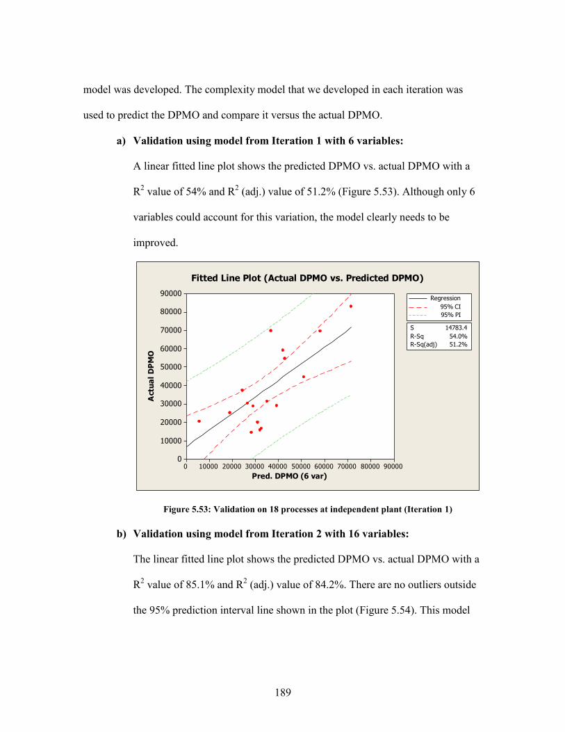
189

model was developed. The complexity model that we developed in each iteration was

used to predict the DPMO and compare it versus the actual DPMO.

a) Validation using model from Iteration 1 with 6 variables:

A linear fitted line plot shows the predicted DPMO vs. actual DPMO with a

R2 value of 54% and R

2 (adj.) value of 51.2% (Figure 5.53). Although only 6

variables could account for this variation, the model clearly needs to be

improved.

9000080000700006000050000400003000020000100000

90000

80000

70000

60000

50000

40000

30000

20000

10000

0

Pred. DPMO (6 var)

Actu

al

DP

MO

S 14783.4

R-Sq 54.0%

R-Sq(adj) 51.2%

Regression

95% CI

95% PI

Fitted Line Plot (Actual DPMO vs. Predicted DPMO)

Figure 5.53: Validation on 18 processes at independent plant (Iteration 1)

b) Validation using model from Iteration 2 with 16 variables:

The linear fitted line plot shows the predicted DPMO vs. actual DPMO with a

R2 value of 85.1% and R

2 (adj.) value of 84.2%. There are no outliers outside

the 95% prediction interval line shown in the plot (Figure 5.54). This model

190

with 16 variables shows a significant improvement as compared to the model

in iteration 1 with 6 variables.

9000080000700006000050000400003000020000100000

90000

80000

70000

60000

50000

40000

30000

20000

10000

0

Predicted DPMO (=33381 + Cd + Cp + Ch)

Actu

al

DP

MO

S 8419.66

R-Sq 85.1%

R-Sq(adj) 84.2%

Regression

95% CI

95% PI

Fitted Line Plot (Iteration 2: Total 16 variables)

Figure 5.54: Validation on 18 processes at independent plant (Iteration 2)

c) Validation using model from Iteration 3 with 24 variables:

The fitted line plot shows the predicted DPMO vs. actual DPMO with a R2

value of 93.7% and R2 (adj.) value of 93.3%. There is one outlier outside the

green 95% prediction interval line shown in the plot (Figure 5.55).

191

9000080000700006000050000400003000020000100000

90000

80000

70000

60000

50000

40000

30000

20000

10000

0

Predicted DPMO (=135,822 + Cd + Cp + Ch)

Actu

al

DP

MO

S 5488.70

R-Sq 93.7%

R-Sq(adj) 93.3%

Regression

95% CI

95% PI

Fitted Line Plot (Iteration 3: Total 24 variables)

Figure 5.55: Validation on 18 processes at independent plant (Iteration 3)

The histogram shows one potential outlier in the data (Figure 5.56). The

normal probability plot shows a linear pattern, consistent with a normal

distribution, again with the same outlier highlighted above (Figure 5.57). The

plot of residual versus fitted values shows a random pattern, which suggests

that the residuals have constant variance (Figure 5.58). Also, the residual

versus order plot shows the order in which the data was collected. It does not

display a pattern which means there is no evidence of non-random error

(Figure 5.59).

192

150001000050000-5000

4

3

2

1

0

Residuals

Fre

qu

en

cy

Histogram of Residuals

Figure 5.56: Histogram of residuals (Source: 18 fastening processes)

150001000050000-5000-10000

99

95

90

80

70

60

50

40

30

20

10

5

1

Residuals

Pe

rce

nt

Mean 1638

StDev 5377

N 18

AD 0.320

P-Value 0.506

Normality Plot (Residuals)Normal

Figure 5.57: Normal probability plot of residual values (p-value = 0.506)

193

9000080000700006000050000400003000020000100000

15000

10000

5000

0

-5000

-10000

-15000

Predicted DPMO

Re

sid

ua

ls

0

Scatterplot of Residuals vs Predicted DPMO

Figure 5.58: Scatter plot of residuals vs. predictor DPMO

18161412108642

15000

10000

5000

0

-5000

-10000

-15000

Observation order

Re

sid

ua

ls

0

Residuals vs. Observation Order

Figure 5.59: Residuals vs. Observation Order plot

194

In summary, the model with 16 variables generated a R2 value of 84.2% (iteration

2) and the model with 24 variables generated a slightly higher R2 value of 93.3%

(iteration 3). Both models were validated successfully at an independent plant that used

mechanical fastening processes for mixed-model automotive assembly.

5.5. Limitations in application of the Hinckley Model to the pilot process

Based on defect data of semiconductor products, Hinckley found that defect per

unit (DPU) was positively correlated with total assembly time and negatively correlated

with number of assembly operations [37]. He defined the assembly complexity factor (Cf)

as follows:

0

0

where,

=Total assembly time for the entire product

=Total number of assembly operations

Threshold assembly time

fC TAT t TOP

TAT

TOP

t

(2.54)

In order to calibrate the correlations between these parameters, Hinckley

incorporated the threshold assembly time (t0) which was defined as the time required to

perform the simplest assembly operation. With this complexity index, Hinckley found

that when plotting on a log-log scale, the complexity and the corresponding defect rate

showed a positive linear correlation with each other, as in the following two equivalent

equations:

log log logf

k

f

DPU k C C

CDPU

C

(2.55)

where, C and k are constants.

195

One of the drawbacks of the Hinckley model is that the predicted quality is for an

entire product. This would enable comparison of complexity and product quality across

multiple entire products. A hypothetical application of the Hinckley Model to two

different vehicles with different total assembly times has been shown in Table 5.6. Model

A requires 26.2 hours for complete assembly and model B requires 24.1 hours for

complete assembly. In Table 5.6, TOP refers to Total number of operations, TAT is the

total assembly time in hours and in seconds, t0 is the threshold time, and Cfpi is the

complexity factor.

Table 5.6: Application of the Hinckley Model to automotive assembly

An example of the complexity calculation has been shown below for Model A:

(93,600) (4 10,000)

53,600

fpi o

fpi

fpi

C TAT t TOP

C

C

(2.56)

According to Hinckley, there is a linear correlation between log(Cfpi) and log(DPU),

where DPU stands for Defects per Unit. However, as shown in Table 5.6, actual DPU for

Model B is 0.7 and that for Model A is 1.2. That is inversely proportional to the

complexity factor that has been calculated for these two models. A modified version of

this model can be applied at a process level, where the time is associated with a certain

process instead of the entire product assembly and the defect rate is associated with the

Ref. TOP

(#)

Takt

Time

(s)

TAT

(hr)

TAT

(s)

t 0

(s)

C fpi

(#)log (C fpi)

Actual

DPUlog (DPU)

Model A 13,920 100 26.2 94,320 4 38,640 4.59 1.2 0.079

Model B 11,620 120 24.1 86,760 4 40,280 4.61 0.7 -0.155

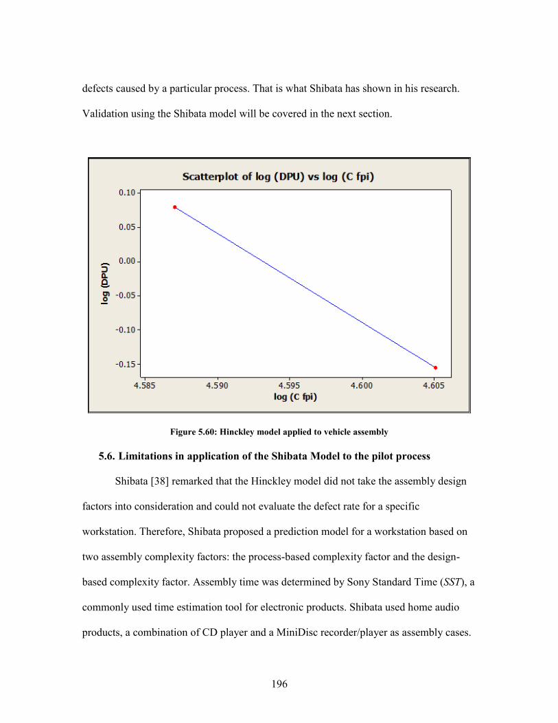
196

defects caused by a particular process. That is what Shibata has shown in his research.

Validation using the Shibata model will be covered in the next section.

Figure 5.60: Hinckley model applied to vehicle assembly

5.6. Limitations in application of the Shibata Model to the pilot process

Shibata [38] remarked that the Hinckley model did not take the assembly design

factors into consideration and could not evaluate the defect rate for a specific

workstation. Therefore, Shibata proposed a prediction model for a workstation based on

two assembly complexity factors: the process-based complexity factor and the design-

based complexity factor. Assembly time was determined by Sony Standard Time (SST), a

commonly used time estimation tool for electronic products. Shibata used home audio

products, a combination of CD player and a MiniDisc recorder/player as assembly cases.

197

These had approximately 300 job elements and the total time was approximately 10

minutes.

The process-based complexity factor of workstation i is defined as:

0

1

0

.

where,

=number of job elements in workstation ;

time spent on job element in workstation ;

threshold assembly time

aiN

Pi ij ai

j

ai

ij

Cf SST t N

N i

SST j i

t

(2.57)

Home audio equipment served as a good vehicle for Shibata’s analysis because its

assembly process contained almost every type of basic assembly operation that is present

in consumer electronic products.

Similar to the Hinckley Model, Shibata derived the following correlation between

the process-based assembly complexity factor and DPU:

logDPU .log logi PiK Cf C (2.58)

DPU

K

Pi

i

Cf

C (2.59)

where C and K are constants.

We apply the Shibata model to the mechanical fastening process to understand the

applicability and gaps, if any. Data for 18 processes from the independent validation

plant is used for this experiment.

198

Table 5.7: Application of Shibata model to mechanical fastening processes

The complexity factor was calculated per the Shibata model. For example, Cfpi for

process number 1 is calculated as follows:

0

1

.

(113.9) (3 16)

65.9

aiN

fpi ij ai

j

fpi

fpi

C SST t N

C

C

(2.60)

As shown in Figure 5.61, the linear model is unable to explain the variation in the

resulting variable (DPMO). Figure 5.62, shows a cubic relationship and that model has a

negligible R2 value as well. Similarly, a quadratic relationship also produced a negligible

R2

value. This shows that although the Shibata model was developed based on data from

several factories where Sony products were built, the model seems to have limited

application to small electronic products such as a MiniDisk Player [37, 38]. The

Ref.No of tasks

in takt (N ai)

Takt

Utilization

%

Opport

unities

per car

Actual

DPMO

Actual

DPU

Takt

Time

(s)

Sum of

time

spent in

takt (s)

t 0

(s)C fpi log (C fpi)

log

(Actual

DPU)

1 16 94.9% 4 44,380 0.18 120 113.9 3 65.9 1.82 -0.75

2 17 66.1% 1 82,799 0.08 120 79.3 3 28.3 1.45 -1.08

3 17 93.6% 1 15,459 0.02 120 112.3 3 61.3 1.79 -1.81

4 17 93.6% 1 22,007 0.02 120 112.3 3 61.3 1.79 -1.66

5 11 87.7% 4 54,350 0.22 120 105.2 3 72.2 1.86 -0.66

6 19 86.7% 5 19,831 0.10 120 104.1 3 47.1 1.67 -1.00

7 25 99.9% 3 24,947 0.07 120 119.8 3 44.8 1.65 -1.13

8 11 95.9% 3 16,465 0.05 120 115.0 3 82.0 1.91 -1.31

9 11 95.9% 3 31,045 0.09 120 115.0 3 82.0 1.91 -1.03

10 17 92.9% 1 58,953 0.06 120 111.4 3 60.4 1.78 -1.23

11 17 92.0% 1 69,390 0.07 120 110.4 3 59.4 1.77 -1.16

12 21 89.7% 5 14,175 0.07 120 107.7 3 44.7 1.65 -1.15

13 18 86.9% 5 28,430 0.14 120 104.3 3 50.3 1.70 -0.85

14 21 95.9% 5 28,834 0.14 120 115.1 3 52.1 1.72 -0.84

15 16 80.6% 1 20,190 0.02 120 96.7 3 48.7 1.69 -1.69

16 15 99.2% 1 30,009 0.03 120 119.0 3 74.0 1.87 -1.52

17 15 99.2% 1 69,314 0.07 120 119.0 3 74.0 1.87 -1.16

18 10 87.7% 4 37,002 0.15 120 105.3 3 75.3 1.88 -0.83

SHIBATA MODEL

199

electronics assembly processes are by no means considered low on the complexity scale

but perhaps the repeatable tasks such as soldering components on printed circuit boards

present a unique set of processes to which this model can be applied and quality can be

reliably predicted.

1.91.81.71.61.51.4

-0.5

-1.0

-1.5

-2.0

log(Cfpi)

log

(DP

U)

S 0.343394

R-Sq 0.0%

R-Sq(adj) 0.0%

Regression

95% CI

95% PI

Fitted Line Plot (Shibata Model - Linear)

Figure 5.61: Fitted Line Plot – Shibata Model (linear)

200

1.91.81.71.61.51.4

0.0

-0.5

-1.0

-1.5

-2.0

-2.5

log(Cfpi)

log

(DP

U)

S 0.362958

R-Sq 2.2%

R-Sq(adj) 0.0%

Regression

95% CI

95% PI

Fitted Line Plot (Shibata Model - Cubic)log(DPU) = - 65.6 + 119.5 log(Cfpi)

- 73.4 log(Cfpi)**2 + 14.92 log(Cfpi)**3

Figure 5.62: Fitted Line Plot - Shibata Model (Cubic)

In published literature [37], we also found a case-study in which Su, Liu, and Whitney

applied the Shibata model to a Fuji photocopier and found R2 values ranging from 0.153

to 0.169 (15.3% to 16.9%). It was found that the Sony Standard Time (SST) database was

not suitable for analyzing the copier production. For instance, the threshold time t0 is 2

seconds in SST while the shortest adjustment action can be completed in 0.6 seconds in

the case of the copier assembly. They also concluded that, “the evaluation method of the

assembly complexity factors should be redesigned to better match the characteristics of a

copier.”

In our study, we also came across an interesting situation that contradicts the

findings from Shibata model. We added a fixture to a fastening operation. Using the new

201

fixture increased the total time. The takt utilization in case 5 [Table 5.7], went up from

87.7% to 93.3%. This increased the Cfpi value from 72.2 to 79. This should have

increased the defect rate. However, the fixture improved the repeatability of the process

and thus reduced the assembly time variation. This finding prompted us to include

Assembly Time Variation as one of the input variables in our complexity model.

5.7. Comparison with proposed Complexity Model

Based on literature review and the gap analysis based on application of existing

models, we defined complexity from a broader view point and included design variables,

process variables, and human-factors. Details of each input variable and the final model

have been described in section 5.4.8. Comparison of the proposed complexity model

(current research) with the complexity factors calculated using the Shibata Model is

shown in Table 5.9.

Linear, quadratic, and cubic regression models were applied to the data and

following R2 values were obtained:

Table 5.8: Summary of R-Sq. values using various regression models

Based on this data, we choose the linear regression model. The fitted line plot is

shown in Figure 5.63.

Regression Model R2

R2 (adj)

Linear 91.9% 91.4%

Quadratic 92.0% 90.9%

Cubic 92.0% 90.3%

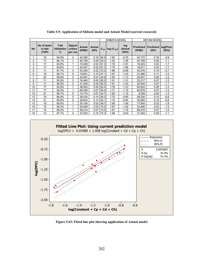
202

Table 5.9: Application of Shibata model and Antani Model (current research)

-0.6-0.8-1.0-1.2-1.4-1.6-1.8

-0.50

-0.75

-1.00

-1.25

-1.50

-1.75

-2.00

log(Constant + Cp + Cd + Ch)

log

(DP

U)

S 0.0975607

R-Sq 91.9%

R-Sq(adj) 91.4%

Regression

95% CI

95% PI

Fitted Line Plot: Using current prediction modellog(DPU) = 0.03480 + 1.008 log(Constant + Cd + Cp + Ch)

Figure 5.63: Fitted line plot showing application of Antani model

No

No of tasks

in takt

(TOP)

Takt

Utilization

%

Opport

unities

per car

Actual

DPMO

Actual

DPUC fpi log (C fpi)

log

(Actual

DPU)

Predicted

DPMO

Predicted

DPU

log(Pred.

DPU)

1 16 94.9% 4 44,380 0.18 65.9 1.82 -0.75 44,172 0.18 -0.8

2 17 66.1% 1 82,799 0.08 28.3 1.45 -1.08 83,789 0.08 -1.1

3 17 93.6% 1 15,459 0.02 61.3 1.79 -1.81 19,525 0.02 -1.7

4 17 93.6% 1 22,007 0.02 61.3 1.79 -1.66 18,611 0.02 -1.7

5 11 87.7% 4 54,350 0.22 72.2 1.86 -0.66 45,276 0.18 -0.7

6 19 86.7% 5 19,831 0.10 47.1 1.67 -1.00 21,686 0.11 -1.0

7 25 99.9% 3 24,947 0.07 44.8 1.65 -1.13 20,561 0.06 -1.2

8 11 95.9% 3 16,465 0.05 82.0 1.91 -1.31 23,317 0.07 -1.2

9 11 95.9% 3 31,045 0.09 82.0 1.91 -1.03 24,045 0.07 -1.1

10 17 92.9% 1 58,953 0.06 60.4 1.78 -1.23 60,624 0.06 -1.2

11 17 92.0% 1 69,390 0.07 59.4 1.77 -1.16 65,678 0.07 -1.2

12 21 89.7% 5 14,175 0.07 44.7 1.65 -1.15 9,208 0.05 -1.3

13 18 86.9% 5 28,430 0.14 50.3 1.70 -0.85 28,326 0.14 -0.8

14 21 95.9% 5 28,834 0.14 52.1 1.72 -0.84 30,650 0.15 -0.8

15 16 80.6% 1 20,190 0.02 48.7 1.69 -1.69 17,654 0.02 -1.8

16 15 99.2% 1 30,009 0.03 74.0 1.87 -1.52 34,488 0.03 -1.5

17 15 99.2% 1 69,314 0.07 74.0 1.87 -1.16 68,916 0.07 -1.2

18 10 87.7% 4 37,002 0.15 75.3 1.88 -0.83 21,558 0.09 -1.1

SHIBATA MODEL ANTANI MODEL

203

In summary, we tested the hypothesis that manufacturing complexity can predict product

quality in mixed-model automotive assembly. The generalized model can be applied to

other processes by identifying the relevant input variables under each of the categories

listed under design complexity, process complexity, and human-factors driven

complexity.

5.8. Error-proofing the process

An important element of process planning is the concept of designing the product

and/or process to be error-free by using Poka-Yoke devices. Poka-Yoke is a Japanese

word that means mistake-proofing and is a key element of the Toyota Production System.

An error-proofing system is economical if it can do the following:

a) Prevent defects that human beings (operators) would otherwise make due

to lack of knowledge, understanding or inadvertence.

b) Provide a solution that would otherwise require significant re-training of

many operators.

c) Bypass complex analysis for causes by finding a solution even though the

cause of the defects remains a mystery [64].

5.8.1. Methods of error-proofing

Some of the usual forms of error-proofing systems / devices are summarized below:

a) Fail-Safe Devices: These devices consist of the one of the following or a

combination of the following mechanisms / systems:

a. Interlocking sequences: Mechanical or electrical logic that ensures that

operation A is performed and subsequent operation B occurs only if

204

operation A has been completed. For example, operation B locates based

on a hole machined in operation A.

b. Alarms and cutoffs: Mechanical or electrical devices that monitor a

certain variable and produce an audible alarm when the monitored variable

falls outside the specification limits or physically stops a process if

programmed as a cutoff device or signal. The alarm would be considered

passive as it still requires intervention to stop the process that can

potentially cause a defect. A cutoff device or signal would be an active

system that can stop the process without additional intervention.

c. All-clear signal: A signal of this nature monitors one or more variables

and provides an audible, visual, or an electrical signal that allows the next

step or process from taking place.

d. Mistake-proof fixtures: These are mechanical devices that may or may

not be integrated with additional sensors (electronic, hydraulic, pneumatic)

that monitor variables such as part features or quality from preceding

operations and allow the next steps of the process to continue only if the

monitored variables meet the specifications. Fixtures may also have

features that prevent the release of a part unless the monitored variable

meets the specifications in the process that was carried out in that specific

process. Manual intervention would be required to release the part, thereby

forcing the operator to recognize that an error has occurred.

205

e. Limiting mechanisms: These devices prevent a monitored variable from

exceeding the predetermined specifications. For example, a slipping-

torque wrench that prevents over-tightening.

b) Magnification of senses: Unlike the fail-safe devices listed above, these types of

devices improve or extend the ability of a human operator to respond before an

error occurs. For example, remote-control monitoring of a closed chamber to

permit viewing despite distance, process temperature, or fumes. Another device in

this category would be one that give multiple signals to improve likelihood of

recognition and response. An example of such an audiovisual signal would be

simultaneous ringing of bells and flashing of lights.

c) Redundancy: This consists of additional work performed purely as a quality

safeguard. “Layered checks” fall under this category in the automotive assembly

industry. Multiple checks are conducted as the vehicle progresses down the

assembly line to catch the same problem if it exists.

d) Audible countdown: Countdowns are arranged by structuring sensing and

information procedures to parallel the operating procedures so that the operational

steps are checked against the sensing and informational needs [64]. For example,

in a manual welding process that requires 18 spot welds, the tool would provide

an audible countdown so that the operator knows clearly when all 18 spot welds

are completed.

5.8.2. Error-Proofing Principles

206

In a classic study, Nakajo and Kume [80] discuss five principles of error-proofing

developed from an analysis of about 1000 examples collected from assembly lines. The

principles, objective, and an example of each are shown in Table 5.10.

Table 5.10: Error-proofing principles

5.8.3. Error-Proofing methods in automotive assembly

Various error-proofing methods are used in automotive assembly based on the

five principles highlighted above. The most common ones are explained below:

1) Visual Display: These are visual monitors that are synchronized with the

database that consists of information about option content and the sequence of

vehicles on the mixed-model assembly line. When the operator has to select a

particular part from a part family of several options, these monitor help the

operator see a number that refers to the part that needs to be assembled in the

vehicle that is at the operator’s station. The monitor can also include a picture

Figure 5.64, color coded logo or any other visual identifier that would help the

operator distinguish the part to be installed from the others on the storage

rack.

Principle Objective Example

Elimination Eliminate possibility of error Redesign process / product

Replacement Substitute current process with a reliable process Robotics in welding

Facilitation Simplify the work Color coded parts

Detection Detect error before further processing Closed loop monitoring and part release

Mitigation Minimize the effect of error Utilize fuses for overloaded circuits

207

Figure 5.64: Visual display to aid component selection

2) Audio Device: An audio device plays a similar role as a visual display by

announcing the component name or code of the part that needs to be installed

in the vehicle that is at the operator’s station. It is also linked to the vehicle

sequencing and option content database. In some cases, quality engineers pair

the audio device along with the visual display and provide an audio-visual

alert to the operator if one of the two is not sufficient to prevent errors.

3) Pick-to-Light system: These systems are typically installed on part racks to

aid selection of the correct part from a set of bins (part containers). The

system is connected to the option content and sequencing database like the

audio-visual systems. A light flashes on top of the bins from where the

components need to be picked up. A sensor is installed on top of every bin to

208

sense the operators hand going into the bin. When a part gets picked up, the

light stops flashing. When all the lights on the rack stop flashing the operator

knows that all the components that needed to be picked up have been removed

from the respective bins Figure 5.65. There are several different variants of

this basic system.

Figure 5.65: Pick-to-light error-proofing system

4) Error-proofing fixtures: As described in the earlier section, fixtures are

generally custom built to develop the error-proofing functionality depending

on the type of error that needs to be prevented. In this research, we designed

and implemented a fixture that reduces tool extension tip play (wobble),

thereby reducing variability in the assembly process. A case-study

highlighting its application will be described in the next chapter.

209

5) Closed-Loop Monitoring: Specifically in the case of controlled mechanical

fastening processes, as described in section 5.3.1, various process parameters

are tracked. Variables such as number of fasteners assembled, torque, angle,

Vehicle Identification Number (VIN), and time stamp are captured by the

monitoring system. When the torque and angle are within specifications,

confirmation LEDs on the tool and the visual display screen turn green, in

order to provide a clear confirmation to the operator about the status of the

assembled fastener. If an error occurs, the operator can attempt the process

one more time. If it fails again, the error code stays associated with the vehicle

and is displayed at the end of every assembly line, all the way to the end of the

final assembly process. Once the fastener is re-worked by the offline operator,

the error needs to be cleared manually from the system to allow final shipment

of the car from the assembly plant.

5.8.4. Incorporating error-proofing systems into predictive model

Process and Quality Engineers in automotive assembly plants focus on processes

that are key drivers of the DPMO metric. Their primary goal is to implement error-

proofing devices to eliminate or significantly reduce the potential for error in those

processes. In our research, we studied various error-proofing devices and their impact on

the predictive model. If the error-proofing device completely eliminates a type of error,

then the input variables associated with that error would basically be reduced to zero. We

conducted various experiments on real-world processes using the predictive model.

210

Highlights of these experiments have been covered in the form of case-studies in the

following chapter.

In conclusion, this chapter addressed research questions two and three. We

developed a generalized model to predict quality based on complexity and applied it to a

specific controlled fastening process. We also determined classes of defect prevention

devices used in automotive assembly and used the model to lower complexity and

improve quality.

211

CHAPTER SIX

6. CASE STUDIES

6.1. Experimental Setup

In order to truly validate the complexity model, we conducted several experiments

to reduce manufacturing complexity. Experiments were done by varying or eliminating

the impact of complexity driving input variables offline on a new test and training station.

This test and training station was developed specifically for this research project with all

the standard equipment used on an assembly line for mechanical fastening.

Figure 6.1: Test Set-up for experimentation and Off-line Training Station

212

Two case-studies have been shown here to highlight the quality improvements

that were made by taking specific steps to reduce complexity driven by design, process,

and human-factors. The results shown here have been sustained for over 6 months since

the time they were first implemented as a trial run on the final assembly line. A third

case-study shows how the model applies to a fully-automated mechanical fastening

process where the human-factors do not play a role.

6.2. Case Study 1: Seat Adapter Assembly Process

6.2.1. Overview of the Seat Adapter assembly process

Seat Adapter is a light weight, hard Styrofoam component that is assembled to the

body inside the passenger cabin. The leather or cloth seat that passengers physically use

gets mounted on top of the Seat Adapter. The tool extension has to be long because it is

used to apply torque to multiple fasteners, including ones that are in the middle of the

seat and are located in deep sockets inside the Styrofoam Seat Adapter (Figure 6.2).

Figure 6.2: Seat Adapter assembly process

213

6.2.2. Problem Description

By nature of the mechanism inside the fastening tool, the output shaft of the tool

vibrates. This vibration is propagated along the length of the extension and results in a

significant amount of play (wobble) at the end of the extension that physically contacts

the torx profile of the fastener. This tip play prevents the operator from aligning the tool

into the head of the fastener promptly and more importantly, results in tool slip-off. This

is a condition in which the tool momentarily loses alignment with the fastener and

thereby drops torque instantaneously (Figure 6.3).

Figure 6.3: Defect caused due to tool slip-off

A diagram showing the total tip play (Pmax) is representative of the fastening process for

the Seat Adapter Figure 6.4.

214

Figure 6.4: Seat Adapter - Tool Tip Play (Pmax)

6.2.3. Complexity and Quality measurement

Total Tip Play is an input variable under the Tooling and Fixture Design category

which falls under the process driven complexity. In the complexity model, Total Tip Play

is captured in millimeters (mm). The coefficient of Total Tip Play in the equation is

690.1.

Values of key parameters before improvement were as follows:

a. DPMO = 76,320

b. Length of extension and driving bit = 241.3 mm

c. Total Tip Play (Pmax)= 51 mm

d. Contribution of Total Tip Play to DPMO = 690.1(51) = 35,195

6.2.4. Implementation of revised process and results

In order to reduce Total Tip Play (wobble), we designed a supporting sleeve with

a needle bearing. This sleeve had a threaded end that would directly fit the threaded end

of the tool where the output shaft is located. The other end of the sleeve had a needle

215

bearing that would support the extension. After three iterations, we developed a sleeve in

the local machine shop that resulted in a Total Tip Play of 2 mm (a reduction of 49 mm).

The operators on the assembly line noticed the difference right away during the trial runs.

We validated the new sleeve offline on the training station and then implemented it on

the assembly line for 2 working shifts (approximately 650 vehicles x 3 fasteners each).

Values of key parameters after improvement were as follows:

a. Length of extension and driving bit = 241.3 mm (un-changed)

b. Total Tip Play = 2 mm

c. Reduction in Total Tip Play = 51 – 2 = 49 mm

d. Predicted DPMO reduction = 690.1 (49) = 33,815

e. Predicted DPMO = 76,230 – 33,815 = 42,415

f. Actual DPMO = 39,280

Figure 6.5: Before and After Process Improvement

6.2.5. Summary

216

This case-study represented a practical implementation of process driven

complexity reduction. The resulting reduction of 48% in DPMO was predicted well by

the complexity model. The improvement was monitored over a period of 6 months and

was successfully sustained.

6.3. Case Study 2: Roof-Rail Assembly Process

6.3.1. Overview of Roof-Rail Assembly Process

Roof-Rails are assembled on top of the roof of a vehicle to hold luggage racks or

other specially designed containers (Figure 6.6).

Figure 6.6: Roof-Rail assembly

In our study, each roof-rail was assembled using three fasteners. The roof-rail

sub-assembly would arrive from the supplier to the final mixed-model vehicle assembly

plant with integrated fasteners. The painted vehicle body has holes in which the roof-rail

is placed. One hole near the A-pillar (hole # 1) of the car is the locating hole, therefore it

is round in shape. There is another hole past the B-pillar (hole # 2) and the third one is

between the C-pillar and the D-pillar (hole # 3). The roof-rail is placed from the top of

the roof by an operator in those three holes. Another operator assembles a nut to each

217

fastener from below the roof and secures the roof-rail to the body, using a mechanical

fastening process.

6.3.2. Problem definition

In the case of the fastener that is closest to the back of the vehicle (# 3), the

fastener visibility is negligible. This is due to the distance between the end of the fastener

and point where the fastening nut has to be installed by the operator from under the roof.

The inner body panel curves away from the roof line which causes the increased distance

resulting in negligible visibility. An actual view of the access hole with a fastener is

shown in Figure 6.7.

Figure 6.7: Actual view of blind hole

The operator uses a tool with a long extension that has a magnetic socket on

which the nut is placed. As the bolt attached to the roof-rail is not visible at all, the

operator uses the long extension to estimate the location of the bolt and drive the nut.

This increases the potential for cross-threading because the nut may not be aligned with

the threads on the bolt. The end result is a torque and angle value that is outside the

specification, causing a defect.

218

6.3.3. Complexity and Quality measurement

Values of key parameters before improvement were as follows:

a. Actual DPMO = 26,210

b. % of fastener invisibility = 100 % (completely blind)

c. Coefficient of fastener visibility variable = 421.6

d. Contribution of lack of fastener visibility to DPMO = 421.6(100) =

42,160

6.3.4. Implementation of revised process and results

In this case the complexity was clearly driven by design factors. Due to limited

access in that area of the vehicle, improving lighting would not improve the ability of the

operator to improve fastener alignment. Therefore, we pursued this as a fastener design

change. In collaboration with the design engineering team, we extended the unthreaded

length of the fastener to provide a guidance path for the tool and nut (Figure 6.8).

Figure 6.8: Fastener design - Before and After Improvement

219

We conducted trial runs with longer fasteners and found that the location ability

and repeatability significantly increased. Therefore, based on feedback from the

operators, we requested the design change.

Values of key parameters after improvement were as follows (Figure 6.9):

a. % of fastener invisibility = 50 % (reduced from 100%)

b. Coefficient of fastener visibility variable = 421.6 (unchanged)

c. Predicted DPMO reduction = 421.6(50) = 21,080

d. Predicted DPMO = 26,210 – 21,080 = 5,130

e. Actual DPMO reduction = 26,210 – 6,570 = 19,640

Figure 6.9: Before and After design improvement

6.3.5. Summary

This case-study represented a practical implementation of design driven

complexity reduction. The resulting reduction of 74% in DPMO was predicted well by

220

the complexity model. The improvement was monitored over a period of 11 months and

was successfully sustained.

6.4. Case Study 3: Fully automated mechanical fastening process

The complexity model in our research is based on design, process, and human-

factors. In a fully automated mechanical fastening process executed by a robot, there

would not be any human intervention unless there is a maintenance issue. This case-study

highlights how the current model applies to a fully automated process if we eliminate the

ergonomic factors which clearly do not apply.

6.4.1. Overview of automated mechanical fastening process

In the automotive assembly world, process of assembling the powertrain and

chassis to the body is called “marriage.” The powertrain and axles are placed on a special

conveying device which has locators to align it to the body. The body is gradually

lowered on the powertrain and the conical locators help align the critical points to ensure

alignment per the required specifications.

Figure 6.10: Fully automated mechanical fastening (powertrain & body)

Once aligned, automated tools assemble 10 critical fasteners on the new assembly

to secure it before allowing it to move to the next station. For our analysis, we choose one

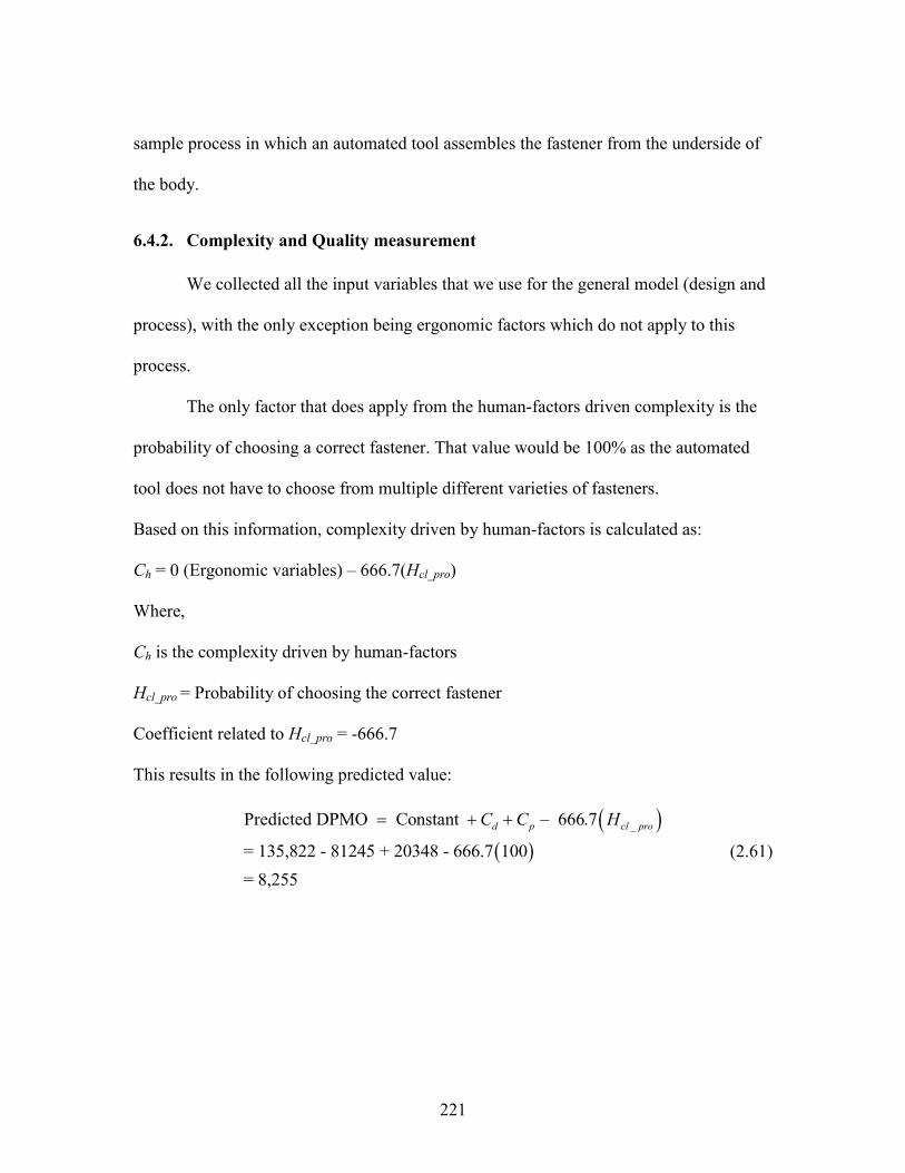
221

sample process in which an automated tool assembles the fastener from the underside of

the body.

6.4.2. Complexity and Quality measurement

We collected all the input variables that we use for the general model (design and

process), with the only exception being ergonomic factors which do not apply to this

process.

The only factor that does apply from the human-factors driven complexity is the

probability of choosing a correct fastener. That value would be 100% as the automated

tool does not have to choose from multiple different varieties of fasteners.

Based on this information, complexity driven by human-factors is calculated as:

Ch = 0 (Ergonomic variables) – 666.7(Hcl_pro)

Where,

Ch is the complexity driven by human-factors

Hcl_pro = Probability of choosing the correct fastener

Coefficient related to Hcl_pro = -666.7

This results in the following predicted value:

_Predicted DPMO Constant – 666.7

= 135,822 - 81245 + 20348 - 666.7 100

= 8,255

d p cl proC C H

(2.61)

222

Figure 6.11: Actual vs. Predicted DPMO (Fully Automated Process)

6.4.3. Summary

This case-study represented a practical application of the complexity model to a

process that was different than the other mechanical fastening processes that were

studied. This process was fully automated; therefore the ergonomic factors did not apply

to prediction of DPMO using the complexity model. The predicted DPMO value was

8,255 versus an actual historical average DPMO value of 9,217. The difference is

statistically negligible and therefore it validates the robustness of the complexity model

from the application standpoint.

223

CHAPTER SEVEN

7. CONCLUSIONS AND FUTURE WORK

7.1. Summary and Conclusions

In this research we successfully tested the hypothesis that manufacturing

complexity can reliably predict product quality in mixed-model automotive assembly.

We proposed a measure of manufacturing complexity that incorporates variables driven

by design, process, and human-factors. In this research, we used controlled mechanical

fastening as a pilot process to demonstrate that manufacturing complexity can reliably

predict product quality in a real-world automotive assembly plant and validated the

mathematical model in an independent assembly plant.

7.1.1. Intellectual Merit

To the best of our knowledge, based on extensive literature review, this is the first

attempt at defining manufacturing complexity using variables driven by design, process,

and human-factors as one comprehensive measure and correlating it to product quality in

a real-world mixed-model assembly system.

The significance of this research includes:

a) Mathematical models that reveal the mechanisms that contribute to

manufacturing complexity in mixed-model assembly systems

b) Assembly time variance as a new measure of complexity versus previous attempts

of considering assembly time and number of assembly operations in a product as

key indicators of product quality

224

c) Application to a real-world process in mixed-model assembly and a research

framework to apply it to another process efficiently

d) Identified a new set of quality driven precedence constraints that will enable

robust assembly line balancing

e) Framework for managing complexity during the design phase for new products as

well as continuous improvement phase in the case of mature products

7.1.2. Broader Impact

The predictive model has the potential to be utilized by design and process

engineers to evaluate the effect of product, process, and human factors on product quality

before implementing the process in a real-world assembly environment. The

methodology used in this research can potentially help develop a new set of constraints

for an optimization model that can be used to minimize manufacturing complexity or

maximize product quality, while satisfying the precedence constraints.

7.2. Future Research

Future research opportunities include the following:

a) Validation of the complexity model and predictive ability by applying this

framework to electrical defects in mixed-model assembly. Electrical defects are

second in line after mechanical fastening based on historical analysis of defects

over one year of production at an assembly plant based in the United States.

b) Although we have shown successful application of this model to fully-automated

mechanical fastening in case-study # 3 (Section 6.4), validating this model across

225

a statistically large sample of fully-automated processes could lead to interesting

outcomes.

c) Test the hypothesis that Assembly Line Balancing with manufacturing complexity

reduction as an objective function results in improved product quality

d) Application of axiomatic design principles to minimize complexity in mixed-

model automotive assembly

7.3. Tools Developed as Part of Research Project

The following tools were developed / built as part of this research work:

a) Mechanical Tools:

i. Training station with closed-loop Atlas Copco torque and angle

monitoring system.

ii. Fixture for the training station to test repeatability of a proposed process

change before implementing it on the assembly line

iii. Sleeve with needle bearing to reduce tip play of the tool extension as

shown in case-study # 1 (section 6.2)

b) Software Tools:

i. VBA based tool to efficiently pre-process defect data for individual

processes from 12 months of historical data

ii. VBA based tool to link defect time stamp with operator / station sign-in

data to identify operator experience level

The mechanical tools that were developed as part of this research are currently being

used by the sponsoring automotive assembly plant where this research was conducted.

226

The software tools will be converted to include a user-friendly user interface and

transferred to the IT department at the sponsoring assembly plant for future use.

7.4. List of Publications

i. Book Chapters:

– Antani, K., “Advances in Mixed-Model Assembly,” in Lean Engineering,

Black, J T., Phillips, D., (Ed.), (ISBN: 978-1621373438) (2013)

ii. Journal Publications:

– Antani, K., Mears, L., Funk, K., Kurz, M., Mayorga, M., 2013, “Manual

Precedence Mapping and Application of a Novel Precedence Relationship

Learning Technique to Real-World Automotive Assembly Line

Balancing,” (J. Manuf. Sci. Eng. – Submitted)

iii. Peer Reviewed Conference Proceedings:

– Antani, K., Pearce, B., Mears, L., K., Kurz, M., Schulte, J., 2014,

“Application of System Learning for Precedence Graph Generation for

Assembly Line Balancing,” Proceedings of the ASME 2014 Intl. Mfg.

Science and Eng. Conference, Detroit, Michigan, 2014-3906 (accepted)

– Antani, K., Mears, L., Funk, K., Kurz, M., Mayorga, M., 2013, “Manual

Precedence Mapping and Application of a Novel Precedence Relationship

Learning Technique to Real-World Automotive Assembly Line

Balancing,” Proceedings of the ASME 2013 Intl. Mfg. Science and Eng.

Conference, Wisconsin, 2013-1235

227

– Antani, K., Mears, L., Funk, K., Kurz, M., Mayorga, M., 2012, “Robust

Work Planning and Development of a Decision Support System for Work

Distribution on a Mixed-Model Automotive Assembly Line,” Proceedings

of the ASME 2012 Intl. Mfg. Science and Eng. Conference, Indiana,

2012-7350

– Antani, K., Black J T., 1999, “Machinability of Gray and Ductile Irons (An

Orthogonal Approach of Experimentation),” SAE Technical Paper, 1999-

01-3378

– Antani, K., Black J T., 1999, “Cellular Manufacturing Insights in Lean

Production Systems,” SAE Technical Paper, 1999-01-3380

iv. Planned Journal Publications (2014-15):

– Antani, K., Mears, L., Kurfess, T., Kurz, M., Mayorga, M., Schulte, J.,

2014, “Effect of manufacturing complexity on product quality in mixed-

model automotive assembly,” (J. Manuf. Sci. Eng.- Submission target

May, 2014)

– Antani, K., Mears, L., Salandro, W., Schulte, J., 2014, “Complexity based

predictive model for assembly of electrical components in powertrain

assembly,” (SAE Intl. J. of Matl. and Mfg.- Submission target Dec, 2014)

– Antani, K., Pearce, B., Mears, L., Kurz, M., Schulte, J., 2014, “Assembly

line balancing to minimize manufacturing complexity and maximize

product quality,” (J. Manuf. Sci. Eng. – Submission target Dec, 2014)

228

– Antani, K., Mears, L., Brooks, J., Schulte, J., 2015, “Human-factors driven

process improvements in high-option powertrain assembly,” (SAE J. of

Matl. and Mfg. – Submission target Mar, 2015)

– Antani, K., Mears, L., Schulte, J., 2014, “Application of axiomatic design

principles to minimize complexity in mixed-model automotive assembly,”

(J. Manuf. Sci. Eng. – Submission target Jul, 2015)

229

REFERENCES

[1] Salveson, M. E., 1955, "The Assembly Line Balancing Problem," The Journal of

Industrial Engineering, pp. 18-25.

[2] Shingo, S., 1989, "A Study of the Toyota Production System from an Industrial

Engineering viewpoint," Productivity Press, Cambridge, MA, pp. 257.

[3] Boysen, N., Fliedner, M., and Scholl, A., 2007, "A Classification of Assembly Line

Balancing Problems," European Journal of Operational Research, 183(2) pp. 674-693.

[4] Shingo, S., 1985, "A Revolution in Manufacturing: The SMED System,"

Productivity Inc., Portland, OR, .

[5] Zhu, X., Hu, S. J., and Marin, S. P., 2008, "Modeling of Manufacturing Complexity

in Mixed-Model Assembly Lines," Journal of Manufacturing Science and Engineering,

130(5) pp. 051013.

[6] Boysen, N., Fliedner, M., and Scholl, A., 2009, "Production Planning of Mixed-

Model Assembly Lines: Overview and Extensions," Production Planning & Control,

20(5) pp. 455-471.

[7] Becker, C., and Scholl, A., 2006, "A Survey on Problems and Methods in

Generalized Assembly Line Balancing," European Journal of Operational Research,

168(3) pp. 694-715.

[8] Antani, K., Kurz, M., Mears, L., 2013, "Manual Precedence Mapping and

Application of a novel precedence relationship learning technique to real-world

230

automotive assembly line balancing." Submitted - Proceedings of the ASME 2013

International Manufacturing Science and Engineering Conference, Madison, Wisconsin.

Anonymous pp. In press.

[9] Ammer, E. D., 1985, "Rechnerunterstützte Planung Von Montageablaufstrukturen

Für Erzeugnisse Der Serienfertigung." IPA-IAO Forschung Und Praxis, 81.

[10] Simon, H. A., 1962, "The Architecture of Complexity," Proceedings of the

American Philosophical Society, 106(6) pp. 467-482.

[11] Blecker, T., 2005, "Information and management systems for product

customization," Springer Science+Business Media, pp. 269.

[12] Deshmukh, A. V., Talavage, J. J., and Barash, M. M., 1998, "Complexity in

Manufacturing Systems, Part 1: Analysis of Static Complexity," IIE Transactions, 30(7)

pp. 645-655.

[13] ElMaraghy, H., 2006, "A complexity code for manufacturing systems," Anonymous

ASME International Conference on Manufacturing Science & Engineeirng (MSEC),

Symposium on Advances in Process & System Planning, Ypsilanti, MI, .

[14] Suh, N.P., 2005, "Complexity: Theory and Applications," Oxford University Press,

New York, NY, .

231

[15] Fisher, M. L., and Ittner, C. D., 1999, "The Impact of Product Variety on

Automobile Assembly Operations: Empirical Evidence and Simulation Analysis,"

Management Science, 45(6) pp. 771-786.

[16] MacDuffie, J. P., Sethuraman, K., and Fisher, M. L., 1996, "Product Variety and

Manufacturing Performance: Evidence from the International Automotive Assembly

Plant Study," Management Science, 42(3) pp. 350-369.

[17] Shimokawa, K., Jurgens, U., and Fujimoto, T., 1997, "Transforming Automobile

Assembly: Experience in Automation and Work Organization," Springer, Berlin, .

[18] Benders, J., and Morita, M., 2004, "Changes in Toyota Motors’ Operations

Management," International Journal of Production Research, 42(3) pp. 433-444.

[19] Nakazawa, H., and Suh, N. P., 1984, "Process Planning Based on Information

Concept," Rob. Computer Integrated Manufacturing, pp. 115-123.

[20] Shannon, C. E., 1948, "A Mathematical Theory of Communication," Bell Systems

Technical Journal, 27pp. 379-423.

[21] Fujimoto, H., and Ahmed, A., 2001, "Entropic Evaluation of Assemblability in

concurrent approach to assembly planning," Proceedings of the IEEE International

Symposium on Assembly and Task Planning, Anonymous Proceedings of the IEEE

International Symposium on Assembly and Task Planning, pp. 306-311.

[22] Suh, N.P., 1990, "The Principles of Design," Oxford University, New York, NY, .

232

[23] Fujimoto, H., Ahmed, A., Iida, Y., 2003, "Assembly Process Design for Managing

Manufacturing Complexities because of Product Varieties," International Journal of

Flexible Manufacturing Systems, 15(4) pp. 283-307.

[24] DeGarmo, E., Black, J., and Kohser, R., 1997, "Materials and Processes in

Manufacturing," Prentice Hall, Upper Saddle River, NJ, pp. 1129-1133.

[25] Gatchell, S. M., 1979, "The Effect of Part Proliferation on Assembly Line

Operators' Decision Making Capabilities," Anonymous Proceedings of the Human

Factors Society, 23rd Annual Meeting, .

[26] Woodworth, R.S., 1938, "Experimental Psychology," Holt, New York, .

[27] Hick, W., 1952, "On the Rate of Gain of Information. ," Quarterly Journal of

Experimental Psychology, 4pp. 11-26.

[28] Hyman, R., 1953, "Stimulus Information as a Determinant of Reaction Time,"

Journal of Experimental Psychology, 45(3) pp. 188-196.

[29] Liu, Y., 1996, "Queuing Network Modeling of Elementary Mental Processes,"

Psychology Rev., 103(1) pp. 116-136.

[30] Plass, J.L., 2010, "Cognitive Load Theory," Cambridge University Press Textbooks,

.

233

[31] Buzzell, R.D., and Gale, B.T., 1987, "The PIMS (Profit Impact of Market Strategy)

Principles-Linking Strategy to Performance," pp. 103-131.

[32] Garvin, D. A., 1987, "Competing for Minimal Maintenance Expense - the Practical

Application of Reliability and Maintainability," Harvard Business Review, pp. 101-109.

[33] Taguchi, G., 1978, "Off-line and on-line quality control systems," Proceedings of

International Conference on Quality, Tokyo, Anonymous .

[34] Shingo, S., 1986, "Zero Quality Control: Source Inspection and Poka-yoke System,"

Productivity Press, Cambridge, MA, .

[35] Rasmussen, J., 1985, "Trends in Human Reliability Analysis," Ergonomics, 28(8)

pp. 1185-1195.

[36] Tsuda, Y., 1993, "Quality through Engineering Design," Elsevier, pp. 79-95.

[37] Qiang Su, Lei Liu, and Whitney, D. E., 2010, "A Systematic Study of the Prediction

Model for Operator-Induced Assembly Defects Based on Assembly Complexity Factors,"

Systems, Man and Cybernetics, Part A: Systems and Humans, IEEE Transactions On,

40(1) pp. 107-120.

[38] Shibata, H., 2002, "Global Assembly Quality Methodology: A New Method for

Evaluating Assembly Complexities in Globally Distributed Manufacturing," ProQuest

Dissertations and Theses, .

234

[39] McCormick, E.J., and Sanders, M.S., 1982, "Human Factors in Engineering and

Design," McGraw-Hill, New York, .

[40] Lewis, H. B., Imada, A. S., and Robertson, M. M., 1988, "Leadership through

quality: merging human factors and safety through employee participation." Human

Factors Society 32nd Annual Meeting, Anonymous Anaheim, CA, pp. 756-759.

[41] Eklund, J. A. E., 1995, "Relationships between Ergonomics and Quality in

Assembly Work," Applied Ergonomics, 26(1) pp. 15-20.

[42] Hancock, W.M., and Bayha, F.H., 1971, ""The Learning Curve", Chapter 4.3,

Handbook of Industrial Engineering," .

[43] Harris, D.H., and Chaney, F.B., 1969, "Human Factors in Quality Assurance,"

Wiley, New York, pp. 9.

[44] Rook, L. W., 1962, "Reduction of Human Error in Production," Sandia National

Laboratories, SC-TM 93-62(14) .

[45] Voegtlen, H., 1988, "Juran's Quality Control Handbook," McGraw-Hill, New York,

pp. 31.1-31.24.

[46] National, R.C., 1991, "Improving Engineering Design-Designing for Competitive

Advantage," National Academy Press, Washington.

235

[47] Hinckley, C. M., 1994, "A Global Conformance Quality Model: A New Strategic

Tool for Minimizing Defects Caused by Variation, Error, and Complexity," ProQuest

Dissertations and Theses, .

[48] Stalk, G., and Hout, T., 1990, "Competing Against Time," Research-Technology

Management, 33pp. 19-24.

[49] Park, K.S., 1987, "Human Reliability - Analysis, Prediction, and Prevention of

Human Errors," Elsevier, Amsterdam, pp. 197.

[50] Brannan, B., 1991, "Six Sigma Quality and DFA-DFMA Case Study/Motorola Inc."

Boothroyd & Dewhurst DFM Insight, 2pp. 1-3.

[51] Boothroyd, G., and Dewhurst, P., 1985, "Product Design for Assembly," Boothroyd

Dewhurst Inc., .

[52] Boothroyd, G., and Knight, W., 1993, "Design for Assembly," Spectrum, IEEE,

30(9) pp. 53-55.

[53] Barkan, P., and Hinckley, C. M., 1993, "Benefits and Limitations of Structured

Methodologies in Product Design," 6(3) pp. 211-219.

[54] Womack, J.P., Daniel, T.J., and Daniel, R., 1990, "The Machine that Changed the

World," Rawson Associates, New York, .

236

[55] Ben-Arieh, D., 1994, "A Methodology for Analysis of Assembly Operations'

Difficulty," International Journal of Production Research, 32(8) pp. 1879.

[56] Wei, C., Chien, C., and Wang, M. J., 2005, "An AHP-Based Approach to ERP

System Selection," International Journal of Production Economics, 96(1) pp. 47-62.

[57] Stillwell, W., von Winterfeldt, D., and John, R. S., 1987, "Comparing Hierarchical

and Non-Hierarchical Weighting Methods for Eliciting Multiattribute Value Models,"

Management Science, 33(2) pp. 442-450.

[58] Webber, S., Apostolou, B., and Hassell, J. M., 1996, "The Sensitivity of the

Analytic Hierarchy Process to Alternative Scale and Cue Presentations<br />," European

Journal of Operational Research, 96(2) pp. 351-362.

[59] Parmley, R.O., 1997, "Standard handbook of fastening and joining," McGraw-Hill,

New York, .

[60] Macduffie, J. P., 1995, "Human Resource Bundles and Manufacturing Performance:

Organizational Logic and Flexible Production Systems in the World Auto Industry,"

Industrial and Labor Relations Review, 48(2) pp. 197-221.

[61] Omar, M.A., 2011, "The Automotive Body Manufacturing Systems and

Processes,"John Wiley & Sons, Ltd, pp. 227-248.

237

[62] Mears, L., Omar, M., and Kurfess, T., 2011, "Automotive Engineering Curriculum

Development: Case Study for Clemson University," Journal of Intelligent Manufacturing,

22(5) pp. 693-708.

[63] Chapman, W., 2004, "Guide to Threads, Threading, and Threaded Fasteners,"

Hanser Gardner, Cincinnati, OH, pp. 596.

[64] Juran, J.M., 1988, "Quality Control Handbook," McGraw-Hill, New York, .

[65] Falck, A., 2010, "The Influence of Poor Assembly Ergonomics on Product Quality:

A Cost-Benefit Analysis in Car Manufacturing," Human Factors and Ergonomics in

Manufacturing & Service Industries, .

[66] Griffin, M., 1997, "Handbook of human vibration," Academic Press, New York, .

[67] Lin, L., 2002, "A Methodology for Incorporating Ergonomics into Manufacturing

Systems Design," Proceedings of the Human Factors and Ergonomics Society Annual

Meeting, 46(13) pp. 1022-1022.

[68] Wickens, C.D., Lee, J.D., Liu, Y., 2004, "An Introduction to Human Factors

Engineering," Pearson Prentice Hall, Upper Saddle River, NJ, pp. 2-3.

[69] Antani, K., Kurz, M., Mears, L., 2012, "Robust Work Planning and Development of

a Decision Support System for Work Distribution on a Mixed-Model Automotive

Assembly Line," Proceedings of the ASME 2012 International Manufacturing Science

and Engineering Conference, Notre Dame, Indiana. Anonymous pp. In press.

238

[70] Poli, C., 2001, "Design for Manufacturing - A Structured Approach," Elsevier, .

[71] Joseph, B. S., and Jimmerson, G., 2012, "Development and Implementation of an

Ergonomics Process in the Automotive Industry ," Occupational Ergonomics, (March)

pp. 571-589.

[72] Argote, L., and Epple, D., 1990, "Learning Curves in Manufacturing," Science,

247pp. 920-924.

[73] Durso, F., 1999, "Handbook of applied cognition," Wiley, New York, .

[74] Wasserman, D.E., 1987, "Handbook of human factors," Wiley, New York, pp. 650-

669.

[75] Fanger, P., 1977, "Thermal Comfort," McGraw Hill, New York, .

[76] Kramer, A. F., Coyne, J. T., and Strayer, D. L., 1993, "Cognitive Function at High

Altitude," Human Factors, 35(2) pp. 329-344.

[77] Boysen, N., Fliedner, M., and Scholl, A., 2009, "Assembly Line Balancing: Joint

Precedence Graphs Under High Product Variety. ," IIE Transactions, 41(3) pp. 183-193.

[78] Weisberg, S., 1980, "Applied Linear Regression," John Wiley & Sons, Inc., .

[79] Neter, J., Kutner, M., Nachtsheim, C., 1990, "Applied Linear Statistical Models,"

Irwin, Chicago, USA, pp. 1408.

239

[80] Nakajo, T., and Kume, H., 1985, "The Principles of Foolproofing and their

Application in Manufacturing," Reports of Statistical Application Research, 32(2) pp. 10-

29.