
A study of reciprocating compressor valve dynamics
104
UNIVERSITY OF WEST BOHEMIA FACULTY OF MECHANICAL ENGINEERING Study Program: N2301 Mechanical Engineering Field of Study: Design of Power Machines and Equipment MASTER THESIS A study of reciprocating compressor valve dynamics Author: Bc. Michal VOLF Supervisor: Doc. Ing. Petr ERET, Ph.D. Academic year 2016/2017
Transcript of A study of reciprocating compressor valve dynamics
UNIVERSITY OF WEST BOHEMIA
FACULTY OF MECHANICAL ENGINEERING
Study Program: N2301 Mechanical Engineering
Field of Study: Design of Power Machines and Equipment
MASTER THESIS A study of reciprocating compressor valve dynamics
Author: Bc. Michal VOLF
Supervisor: Doc. Ing. Petr ERET, Ph.D.
Academic year 2016/2017

University of West Bohemia, Faculty of Mechanical Engineering Master thesis, 2016/2017
Department of Power System Engineering Bc. Michal Volf

University of West Bohemia, Faculty of Mechanical Engineering Master thesis, 2016/2017
Department of Power System Engineering Bc. Michal Volf
Declaration
I hereby declare that this master thesis is entirely my own work and that I only used the
cited sources.
Pilsen, June 2, 2017
___________________________

University of West Bohemia, Faculty of Mechanical Engineering Master thesis, 2016/2017
Department of Power System Engineering Bc. Michal Volf
Acknowledgement
I would like to express my very profound gratitude to my supervisor, Petr Eret for the
useful comments, remarks and engagement from the beginning to the very end of my
master thesis. I truly appreciate his helpful advice and generous help.
Furthermore, my deepest and sincere gratitude goes to my family for their unflagging and
unparalleled love, help and support throughout my life and my studies.
Finally, I would like to thank Richard Pisinger for correcting the English language of
this thesis.

University of West Bohemia, Faculty of Mechanical Engineering Master thesis, 2016/2017
Department of Power System Engineering Bc. Michal Volf
ANOTAČNÍ LIST DIPLOMOVÉ PRÁCE
AUTOR Příjmení
Bc. Volf
Jméno
Michal
STUDIJNÍ OBOR N2301 Strojní inženýrství
VEDOUCÍ PRÁCE Příjmení
Doc. Ing. Eret, Ph.D.
Jméno
Petr
PRACOVIŠTĚ ZČU – FST – KKE
DRUH PRÁCE DIPLOMOVÁ BAKALÁŘSKÁ Nehodící se
škrtněte
NÁZEV PRÁCE Studie dynamiky ventilu u pístového kompresoru
FAKULTA strojní KATEDRA KKE ROK ODEVZDÁNÍ 2017
POČET STRAN (A4 a ekvivalentů A4)
CELKEM 103 TEXTOVÁ ČÁST 82 GRAFICKÁ ČÁST 0
STRUČNÝ POPIS
Diplomová práce se zaměřuje na jednodimenzionální studium
dynamického chování ventilu pístového kompresoru. Za tímto
účelem byl vytvořen program, pomocí nějž jsou kvalitativně
hodnoceny jednotlivé projevy dynamického chování a jejich
vzájemný vliv. Matematický model, jenž je v tomto programu
implementován, je v práci rovněž detailně popsán.
KLÍČOVÁ SLOVA pístový kompresor, dynamika ventilu, interakce těleso-tekutina,
proudění vzduchu, jednodimenzionální model

University of West Bohemia, Faculty of Mechanical Engineering Master thesis, 2016/2017
Department of Power System Engineering Bc. Michal Volf
SUMMARY OF DIPLOMA SHEET
AUTHOR Surname
Bc. Volf
Name
Michal
FIELD OF STUDY N2301 Mechanical Engineering
SUPERVISOR Surname
Doc. Ing. Eret, Ph.D.
Name
Petr
INSTITUTION ZČU - FST - KKE
TYPE OF WORK DIPLOMA BACHELOR Delete when not
applicable
TITLE OF THE WORK A study of reciprocating compressor valve dynamics
FACULTY Mechanical
Engineering DEPARTMENT KKE SUBMITTED IN 2017
NUMBER OF PAGES (A4 and eq. A4)
TOTALLY 103 TEXT PART 82 GRAPHICAL PART 0
BRIEF DESCRIPTION
This master thesis is focused on one-dimensional study of
reciprocating compressor valve dynamics. For this purpose, a
tool was developed, which is used to qualitatively evaluate the
individual aspects of valve dynamics as well as their interaction.
A mathematical model, which is implemented in the tool, is
described in detail in this thesis.
KEY WORDS reciprocating compressor, valve dynamics, flow-structure
interaction, gas flow, one-dimensional model

University of West Bohemia, Faculty of Mechanical Engineering Master thesis, 2016/2017
Department of Power System Engineering Bc. Michal Volf
Table of Contents
Introduction ..................................................................................................................................... 1
1 Research Outline .................................................................................................................... 2
1.1 Motivation of Research ................................................................................................... 2
1.2 Survey of Literature ........................................................................................................ 5
1.3 Purpose of Research ........................................................................................................ 7
2 Compressor Valves ................................................................................................................ 9
2.1 Self-acting and Mechanically Operated Valves .......................................................... 9
2.2 Automatic Valve Types ................................................................................................ 10
2.2.1 Poppet Valve .......................................................................................................... 10
2.2.2 Ring Valve .............................................................................................................. 11
2.2.3 Plate Valve .............................................................................................................. 11
2.3 Valve Design Terminology .......................................................................................... 12
3 The Model .............................................................................................................................. 14
3.1 Overview of the Model ................................................................................................. 14
3.1.1 Processes and Effects to be Simulated ................................................................ 14
3.1.2 The Model Structure ............................................................................................. 15
3.1.3 Simplifying Assumptions ..................................................................................... 17
3.2 Crank Mechanism ......................................................................................................... 18
3.3 Cylinder .......................................................................................................................... 20
3.3.1 Simplifying assumptions ...................................................................................... 20
3.3.2 General Governing Equations ............................................................................. 21
3.3.3 Suction Phase ......................................................................................................... 22
3.3.4 Discharge Phase ..................................................................................................... 24
3.3.5 Expansion and Compression ............................................................................... 24
3.4 Suction and Discharge Valve ....................................................................................... 25
3.4.1 Simplifying assumptions ...................................................................................... 25
3.4.2 Valve Flow Modeling ............................................................................................ 26
3.4.3 Valve Dynamics ..................................................................................................... 28
3.4.3.1 The Mass of the System .................................................................................... 29
3.4.3.2 Spring Force ....................................................................................................... 30
3.4.3.3 Valve Plate Impacts ........................................................................................... 30
3.4.3.4 Friction Force ..................................................................................................... 31
3.4.3.5 Adhesion ............................................................................................................. 31
3.4.3.6 Fluid-Structure Interaction ............................................................................... 33
3.5 Piping System ................................................................................................................ 34
3.6 Periodical Quantities ..................................................................................................... 37
3.6.1 Indicated Work ...................................................................................................... 37
3.6.2 Indicated Valve Work ........................................................................................... 37
3.6.3 Volumetric Efficiency ............................................................................................ 38

University of West Bohemia, Faculty of Mechanical Engineering Master thesis, 2016/2017
Department of Power System Engineering Bc. Michal Volf
3.7 Summary of the Mathematical Model ........................................................................ 38
3.7.1 Suction Phase ......................................................................................................... 38
3.7.2 Discharge Phase ..................................................................................................... 40
3.7.3 Valves Closed ......................................................................................................... 41
3.7.4 Conditions for Transition ..................................................................................... 41
3.7.5 Input Parameters ................................................................................................... 42
4 Developing the Simulation Tool ....................................................................................... 43
4.1 General Remarks ........................................................................................................... 43
4.1.1 Simulation Tool Requirements ............................................................................ 43
4.1.2 Object-Oriented Programming ............................................................................ 44
4.1.3 Structure of the Tool ............................................................................................. 45
4.2 Class Structure ............................................................................................................... 45
4.2.1 Class Properties ..................................................................................................... 45
4.2.2 Class Methods ........................................................................................................ 46
4.2.2.1 Class Constructor .............................................................................................. 47
4.2.2.2 Get-access Methods ........................................................................................... 47
4.3 Solving the Compressor Cycle and Valve Dynamics ............................................... 49
4.3.1 Switching Between Compressor Phases............................................................. 51
4.3.2 Integration of ODEs .............................................................................................. 55
4.3.2.1 Numerical Method of Integration ................................................................... 55
4.3.2.2 Defining Unknown Variables and Equations................................................ 57
4.3.2.3 Initial Conditions ............................................................................................... 57
4.4 Running the Simulation Tool ....................................................................................... 58
4.4.1 Command Line ...................................................................................................... 58
4.4.2 Graphical User Interface ....................................................................................... 59
5 Results of the Simulation ................................................................................................... 61
5.1 Reference Compressor Configuration ........................................................................ 61
5.1.1 Variables as a Function of the Crank Angle ...................................................... 61
5.1.2 Indicator Diagram ................................................................................................. 63
5.1.3 Comparison of the Results ................................................................................... 64
5.1.4 Accuracy of the Results ........................................................................................ 66
5.2 Modified Compressor Parameters .............................................................................. 68
5.2.1 Sensitivity Analysis ............................................................................................... 68
5.2.2 Individual Phenomena Effect .............................................................................. 72
5.2.3 Varying Design Parameters ................................................................................. 76
Conclusion ..................................................................................................................................... 82
A Default Compressor Setup ............................................................................................... A-1
B Content of the DVD ........................................................................................................... B-1

University of West Bohemia, Faculty of Mechanical Engineering Master thesis, 2016/2017
Department of Power System Engineering Bc. Michal Volf
Table of Figures
Figure 1 Sketch of a single-acting reciprocating compressor [41] ........................................ 2
Figure 2 Causes of unscheduled compressor shutdowns [3] ............................................... 3
Figure 3 Impact failure of valve plate caused by stiction [5] ................................................ 4
Figure 4 Spring failure due to abrasive wear [5] .................................................................... 4
Figure 5 Valve ring subject to heavy wear due to the deposition of coke particles [42] ... 4
Figure 6 Timeline of evolution of valve design methods ...................................................... 5
Figure 7 The influence of pressure ratio on compressor cycle ............................................. 9
Figure 8 Poppet valve [40] ....................................................................................................... 11
Figure 9 Ring valve [40] ........................................................................................................... 11
Figure 10 Plate valve [40] ....................................................................................................... 12
Figure 11 Generic model of a valve assembly .................................................................... 12
Figure 12 Ideal and real valve plate lift ............................................................................... 14
Figure 13 Compressor model ................................................................................................ 16
Figure 14 Schematic drawing of the crank mechanism ..................................................... 18
Figure 15 Control volume for compressor cylinder – suction phase ............................... 22
Figure 16 Control volume for compressor cylinder - discharge phase ........................... 24
Figure 17 LES simulation of gas flow through the compressor reed valve [43] ............ 26
Figure 18 Diagram of a generic valve and its replacement by a nozzle .......................... 26
Figure 19 Force balance on valve plate ................................................................................ 28
Figure 20 Effective spring mass ............................................................................................ 29
Figure 21 Linear spring characteristic .................................................................................. 30
Figure 22 Stiction..................................................................................................................... 32
Figure 23 Generic piping system .......................................................................................... 34
Figure 24 Helmholtz resonator concept ............................................................................... 35
Figure 25 Suction plenum chamber ...................................................................................... 36
Figure 26 Discharge plenum chamber ................................................................................. 36
Figure 27 Structure of the compressor class ........................................................................ 46
Figure 28 Class constructor (function syntax) .................................................................... 47
Figure 29 Get-access method for cylinder volume ............................................................. 48
Figure 30 Get-access method for piston displacement ...................................................... 48
Figure 31 Resulting equation for cylinder volume ............................................................ 48
Figure 32 Get-access method for friction force (suction valve) ........................................ 48
Figure 33 Get-access method for condition to move onto the suction phase ................. 49
Figure 34 Functional diagram of solving cycle & valve dynamics .................................. 50
Figure 35 Continuous & numerical solution ....................................................................... 52
Figure 36 Process of integration of ODEs ............................................................................ 55
Figure 37 Function syntax of ode45 ...................................................................................... 55
Figure 38 Schematic process of integration ......................................................................... 56
Figure 39 Variable structure array replacement by a vector............................................. 57

University of West Bohemia, Faculty of Mechanical Engineering Master thesis, 2016/2017
Department of Power System Engineering Bc. Michal Volf
Figure 40 Example of starting the application through set of commands ...................... 58
Figure 41 Home page of the application ............................................................................. 59
Figure 42 Valve dynamics page of the application ............................................................ 60
Figure 43 Settings tab of the application ............................................................................. 60
Figure 44 Results of the simulation for a default compressor setup ............................... 62
Figure 45 Indicator diagram for the default compressor setup ........................................ 64
Figure 46 Comparison of the experimental and theoretical results ................................. 65
Figure 47 Output of valve behavior simulator - Dott. Ing. Mario Cozzani Srl [44] ....... 66
Figure 48 Output from the developed simulation tool ..................................................... 66
Figure 49 Comparison of the solution from different ode solvers ................................... 67
Figure 50 Compressor cycles prior to convergent solution .............................................. 68
Figure 51 Sensitivity analysis for the gas coefficient 𝑐𝑔 ..................................................... 71
Figure 52 Influence of adhesion ............................................................................................ 72
Figure 53 Influence of friction ............................................................................................... 72
Figure 54 Influence of rebound ............................................................................................. 73
Figure 55 Influence of piping systems ................................................................................. 74
Figure 56 Pressure pulsations in case of half-volume plenum chambers ....................... 75
Figure 57 Recording of pressure pulsations by Jaspers [38] ............................................. 75
Figure 58 Recordings of pressure pulsations by Bráblík [32] ........................................... 75
Figure 59 Influence on the periodical results ...................................................................... 76
Figure 60 p-V diagrams - various discharge pressures ..................................................... 77
Figure 61 Valve lift - various discharge pressures ............................................................. 77
Figure 62 Impact velocities - various discharge pressures................................................ 77
Figure 63 Periodical quantities - various discharge pressures ......................................... 78
Figure 64 Valve movement under various compressor speeds ....................................... 78
Figure 65 Impact velocities - various compressor speeds ................................................. 79
Figure 66 Periodical quantities - various compressor speeds........................................... 79
Figure 67 Valve movement under various maximum discharge valve lifts .................. 81
Figure 68 Pressure in the cylinder under various maximum discharge valve lifts ....... 81

University of West Bohemia, Faculty of Mechanical Engineering Master thesis, 2016/2017
Department of Power System Engineering Bc. Michal Volf
Table of Tables
Table 1 Operating conditions for different valve types [18] ............................................. 10
Table 2 System of ODEs - suction phase .............................................................................. 39
Table 3 Time-dependent variables - suction phase ............................................................ 39
Table 4 System of ODEs - discharge phase.......................................................................... 40
Table 5 Time-dependent variables - discharge phase ........................................................ 40
Table 6 System of ODEs – closed valves .............................................................................. 41
Table 7 Conditions for transition .......................................................................................... 41
Table 8 Input parameters ....................................................................................................... 42
Table 9 Numerical representation of compressor phase ................................................... 51
Table 10 Condition for transitions - property names & equations ..................................... 52
Table 11 Modified conditions for transition .......................................................................... 53
Table 12 Conditions for rebound ............................................................................................ 54
Table 13 Comparison of periodical quantities - different ode solvers ............................... 67

University of West Bohemia, Faculty of Mechanical Engineering Master thesis, 2016/2017
Department of Power System Engineering Bc. Michal Volf
List of Abbreviations
Acronym Definition
BDC bottom dead center
CFD computational fluid dynamics
CV control volume
LES large eddy simulation
ODE ordinary differential equation
OOP object-oriented programming
TDC top dead center

University of West Bohemia, Faculty of Mechanical Engineering Master thesis, 2016/2017
Department of Power System Engineering Bc. Michal Volf
List of Frequently Used Symbols
Symbol Unit Property
𝛼 [−] flow coefficient
𝛽 [°] meniscus contact angle
𝛾𝐿𝐺 [𝑁𝑚−1] surface tension
𝜖 [−] expansion coefficient
Θ𝑐𝑑 [𝑘𝑔 𝑠−1] mass flow in discharge valve
Θ𝑐𝑠 [𝑘𝑔 𝑠−1] mass flow in suction valve
Θ𝑑 [𝑘𝑔 𝑠−1] mass flow in discharge pipe
Θ𝑠 [𝑘𝑔 𝑠−1] mass flow in suction pipe
𝜅 [−] heat capacity ratio (Poisson constant)
𝜉 [−] loss coefficient in pipe
𝜌𝑐 [𝑘𝑔 𝑚−3] density of gas inside cylinder
𝜌𝑑 [𝑘𝑔 𝑚−3] density of gas inside discharge chamber
𝜌𝑠 [𝑘𝑔 𝑚−3] density of gas inside suction chamber
𝜙 [°] crank angle
𝜔 [𝑟𝑎𝑑 𝑠−1] angular velocity of crankshaft
𝐴𝑐 [𝑚2] cross-sectional area of cylinder
𝐴𝑜 [𝑚2] flow area
𝐴𝑝 [𝑚2] valve port cross-sectional area
𝐴𝑣 [𝑚2] valve plate area
𝑐𝑓 [𝑁𝑠𝑚−1] friction coefficient
𝑐𝑝 [𝐽𝑘𝑔−1𝐾−1] heat capacity at constant pressure
𝑐𝑟 [−] coefficient of restitution
𝑐𝑣 [𝐽𝑘𝑔−1𝐾−1] heat capacity at constant volume
𝐷𝑐 [𝑚] cylinder diameter
𝐷𝑝 [𝑚] valve port diameter
𝐷𝑣 [𝑚] valve plate diameter
𝐸𝐶𝑉 [𝐽] energy of fluid inside control volume
𝐹𝑎𝑑ℎ [𝑁] adhesion force
𝐹𝑓 [𝑁] fluid friction force
𝐹𝑔 [𝑁] gas force

University of West Bohemia, Faculty of Mechanical Engineering Master thesis, 2016/2017
Department of Power System Engineering Bc. Michal Volf
𝐹𝑠 [𝑁] spring force
ℎ [𝑚] maximum valve plate lift
ℎ𝑓𝑖𝑙𝑚 [𝑚] oil film thickness
𝑘 [𝑁𝑚−1] spring stiffness
𝐿 [𝑚] connecting rod length
𝑚 [𝑘𝑔] mass of valve plate with equivalent mass of spring
𝑚𝑐 [𝑘𝑔] mass of gas inside cylinder
𝑚𝑝𝑙𝑎𝑡𝑒 [𝑘𝑔] valve plate mass
𝑚𝑠𝑝𝑟𝑖𝑛𝑔 [𝑘𝑔] spring mass
𝑝𝑐 [𝑃𝑎] pressure in cylinder
𝑝𝑑 [𝑃𝑎] pressure in discharge chamber
𝑝𝑠 [𝑃𝑎] pressure in suction chamber
�̇� [𝑊] rate of total heat transfer
𝑟 [𝐽𝑘𝑔−1𝐾−1] specific ideal gas constant
𝑅 [𝑚] radius of crankshaft
𝑅𝑒 [−] Reynolds number
𝑡 [𝑠] time
𝑇𝑐 [𝐾] temperature of gas in cylinder
𝑇𝑑 [𝐾] temperature of gas in discharge chamber
𝑇𝑠 [𝐾] temperature of gas in suction chamber
𝑢 [𝐽𝑘𝑔−1] specific internal energy
𝑣𝑐 [𝑚3𝑘𝑔−1] specific volume of gas inside cylinder
𝑣𝑑 [𝑚3𝑘𝑔−1] specific volume of gas inside discharge chamber
𝑣𝑠 [𝑚3𝑘𝑔−1] specific volume of gas inside suction chamber
𝑊 [𝐽] work
𝑤𝑧 [𝑚𝑠−1] piston velocity
𝑥 [𝑚] valve plate lift
𝑥0 [𝑚] spring preload deflection
𝑧 [𝑚] piston displacement
𝑧0 [𝑚] smallest distance between cylinder and piston (derived
from clearance volume)

University of West Bohemia, Faculty of Mechanical Engineering Master thesis, 2016/2017
Department of Power System Engineering Bc. Michal Volf
1
Introduction
Reciprocating compressors are among the most used types of compressors. They can be
found in highly diverse fields of application, such as in the oil and gas industry or chemical
industry, where these compressors are used mainly for their ability to deliver high-pressure
gas. Basically, piston compressors are vital part in any process they are employed in;
therefore their reliability has garnered widespread interest.
As the limiting elements in the design of the reciprocating compressor, the compressor
valves can be considered. They are often described as the heart of the compressor, due to
the fact that should they fail, it would lead to the shutdown of the compressor and to costly
downtimes. A compressor running at even moderate speeds such as 700 rpm requires for
each valve to open and close over one million times a day. It follows that valve design must
bear in mind that it needs to be highly reliable and operate efficiently even in adverse
conditions, such as in applications where there are liquids and debris in the gas stream.
The fundamental challenge in the design of a compressor valve lies in the opening and
closing phase of the valve, where an effort is made to allow for the most desirable dynamic
behavior as possible. For instance, lowering the pressure loss across the valve by increasing
the flow area leads to a higher possibility of unsuitable dynamic behavior and thus
decreases its lifetime.
This thesis is devoted to a theoretical study of reciprocating compressor valve dynamics.
For this purpose, a tool for the prediction of valve plate motion is developed. The main
reason in developing this tool is to qualitatively assess the factors influencing the dynamic
behavior. To validate the precision of this tool, the results are compared to freely accessible
experimental data found in literature. However, the main goal of this study is not aimed at
a quantitative estimation, since an experiment would be inevitable for the precise
evaluation of the theoretical results.
This thesis consists of five parts. The first part deals with the motivation and the purpose
of this research, whereas the second part is meant to provide the general overview of
compressor valves used today. The third part describes the physical model of the
reciprocating compressor and its valves. Based on this, simplifications are introduced and
a mathematical model is proposed. The fourth part is concerned with the implementation
of the mathematical model in the proprietary software MATLAB. In the fifth part, the
results of the developed tool are discussed. The analysis of the influence of the valve
parameters on its dynamic behavior is also present in this chapter.

University of West Bohemia, Faculty of Mechanical Engineering Master thesis, 2016/2017
Department of Power System Engineering Bc. Michal Volf
2
1 Research Outline
1.1 Motivation of Research
A reciprocating or piston compressor (Figure 1) is a compressor that is piston-driven by a
crankshaft in order to deliver high-pressure gas. The compressor captures a volume of gas
from a suction port and transfers it into a cylinder, where it is trapped and compressed by
a piston that reduces its volume. Thereafter, the compressed gas is discharged through the
exhaust port into the discharge pipe. The flow of the gas through the cylinder is controlled
by valves.
Piston compressors are widely employed in several industry and transportation branches
as well as for domestic purposes. Even though they are not able to deliver the compressed
gas continuously, which can be considered as one of their main drawbacks, since it leads to
pressure pulsations in the suction and discharge pipes, their main advantage is the ability
to achieve high pressure ratios (up to 2 500 [1]) and can therefore deliver gases at very high
pressures. According to Ninković [2], an example of such an application involves
compressing ethylene to pressures over 300 MPa to produce LDPE (low-density-
polyethylene). Other typical applications include the compression of gases contaminated
with particles, or gases with very low suction temperatures (down to -150 °C) in the field
of liquefied gas transport and storage.
From the above, it can be freely stated that some of the applications would hardly be
possible without this type of compressor. We can consider the compressor to be the heart
of an installation, as its reliability determines the safety and availability of the entire plant.
Despite there being a requirement of trouble-free operations for several years of operation,
Figure 1 Sketch of a single-acting reciprocating compressor [41]

University of West Bohemia, Faculty of Mechanical Engineering Master thesis, 2016/2017
Department of Power System Engineering Bc. Michal Volf
3
compressors are very complex machines, a consequence of which is that unscheduled costly
shutdowns can happen. An industrial investigation to identify and evaluate the factors of
these shutdowns was conducted by the company Dresser-Rand [3]. The summary of these
results is shown in Figure 2.
Figure 2 Causes of unscheduled compressor shutdowns [3]
Even though the investigation only shows the reliability of an operating piston compressor
and does not take into account a human error, the results clearly identify compressor valves
as the main cause of unscheduled shutdowns, with a relative rate of 36%.
As Ninković [2] points out, in view of the fact that the second-major cause of compressor
failure, the piston rod packing, is only present in compound and crosshead machines, one
may surmise that valves are responsible for an even larger percentage of failure in small
compressors. This underscores the idea outlined in the introduction that valves really are
the heart of the compressor and proper care in their design is not only desired, but it is
decidedly obligatory.
Dresser-Rand [3] states that among the most common causes of valve failures are high
impact velocities, wear, corrosion, and application conditions. Below, we will proceed to
outline how valve dynamics is involved in these causes of failure.
The moving element of the valve is limited in its motion by a seat and a guard. Every time
the valve opens or closes, the moving element strikes the seat or guard. A rebound may
occur if the velocity at the moment of impact is sufficiently high. This behavior is
undesirable, for it leads to a higher dynamic stress of valve parts, resulting in chipping and
cracks on the outer edge of the moving element as well as on the seat and guard (an example
is given in Figure 3).
36.0%
17.8%
8.8%7.1% 6.8% 6.8%
5.1% 5.1%3.4%
1.3% 0.7% 0.4% 0.3% 0.2% 0.2%0%
5%
10%
15%
20%
25%
30%
35%
40%
Per
cen
tage
[%
]

University of West Bohemia, Faculty of Mechanical Engineering Master thesis, 2016/2017
Department of Power System Engineering Bc. Michal Volf
4
Since moving parts of the valve impact and slide against one another, a certain amount of
wear is inevitable (examples are given in Figure 4 and Figure 5). Nevertheless, the wear rate
does not solely depend on proper maintenance e.g. lubrication, but it also depends on the
dynamic behavior of the valves. Moreover, there are pressure pulsations in the suction and
discharge chambers as well as the flutter of the moving element, which can increase the
wear rate and therefore decrease the time until failure.
If the corrosive elements are present in the compressed gas, they might bring about the
corrosion of the valve parts. This is especially dangerous to the springs as they can fail
prematurely due to the corrosion-related fatigue. However, if the gas composition is known
during the design process, suitable corrosive resistant materials can be chosen and therefore
the effects of the corrosion can be limited.
The application conditions refer mostly to the quality of the compressed gas. The presence
of dirt or debris will accelerate wear, can limit opening and closing of the valve, and in
extreme conditions, the valves can become blocked.
In view of the foregoing, it is obvious that rebound, stiction and other effects of valve
dynamics play a vital role in the manner of their failure that can lead to the costly downtime
of the entire plant. The study and deeper understanding of valve dynamics is necessary so
as to further improve the design of the valve and thus the reliability of the compressor.
Figure 4 Spring failure due to abrasive wear [5] Figure 3 Impact failure of valve plate caused by stiction [5]
Figure 5 Valve ring subject to heavy wear due to the deposition of coke particles at the valve seats [42]
University of West Bohemia, Faculty of Mechanical Engineering Master thesis, 2016/2017
Department of Power System Engineering Bc. Michal Volf
5
It should be also emphasized that the economic effect of valve design improvement can be
very significant. According to Howes [4], a comparison of two valves with different valve
lifts shows that for the lower lift version, the revenue1 is higher, while operations and
maintenance costs are slightly lower. Under the given circumstances of the calculation, he
concluded that by optimizing the valve, the net profit could be increased by over half a
million dollars per year.
1.2 Survey of Literature
Despite the long history of piston compressors dating back to 1777, when James Watt
constructed a steam-driven air compressor, valve design was hardly mentioned in
literature until the very beginning of the 20th century. However, the first attempts to
describe valve behavior were purely empirical, even though experimental methods for
recording the valve behavior, e.g. measuring its lift as a function of time, hardly existed.
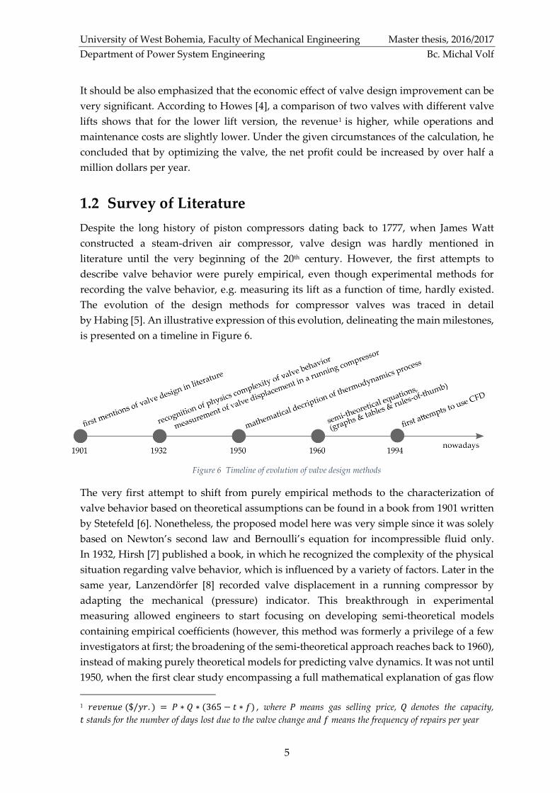
The evolution of the design methods for compressor valves was traced in detail
by Habing [5]. An illustrative expression of this evolution, delineating the main milestones,
is presented on a timeline in Figure 6.
The very first attempt to shift from purely empirical methods to the characterization of
valve behavior based on theoretical assumptions can be found in a book from 1901 written
by Stetefeld [6]. Nonetheless, the proposed model here was very simple since it was solely
based on Newton’s second law and Bernoulli’s equation for incompressible fluid only.
In 1932, Hirsh [7] published a book, in which he recognized the complexity of the physical
situation regarding valve behavior, which is influenced by a variety of factors. Later in the
same year, Lanzendörfer [8] recorded valve displacement in a running compressor by
adapting the mechanical (pressure) indicator. This breakthrough in experimental
measuring allowed engineers to start focusing on developing semi-theoretical models
containing empirical coefficients (however, this method was formerly a privilege of a few
investigators at first; the broadening of the semi-theoretical approach reaches back to 1960),
instead of making purely theoretical models for predicting valve dynamics. It was not until
1950, when the first clear study encompassing a full mathematical explanation of gas flow
1 𝑟𝑒𝑣𝑒𝑛𝑢𝑒 ($/𝑦𝑟. ) = 𝑃 ∗ 𝑄 ∗ (365 − 𝑡 ∗ 𝑓) , where 𝑃 means gas selling price, 𝑄 denotes the capacity,
𝑡 stands for the number of days lost due to the valve change and 𝑓 means the frequency of repairs per year
Figure 6 Timeline of evolution of valve design methods

University of West Bohemia, Faculty of Mechanical Engineering Master thesis, 2016/2017
Department of Power System Engineering Bc. Michal Volf
6
through the valves and of the thermodynamic process in a compressor cylinder appeared
in a book by Costagliola [9]. Since 1994, computational fluid dynamics (CFD) has been used
as a valuable tool for the analysis of compressor valves.
Our research of the recent literature on valve design shows that there is a rapidly growing
number of literature these days, but mainly in the form of conference proceedings, namely
from:
• International Compressor Engineering Conference at Purdue University
• International Conference on Compressors and their Systems of IMechE and City
University in London
• European Forum for Reciprocating compressors
Somewhat surprising is the fact that, despite the compressor manufacturers’ financial
sponsorship of these conferences, much of the proceedings come from scientific researchers
in universities. Furthermore, in view of the fact that only a few of these proceedings clearly
state that the research was made in cooperation with a compressor manufacturer, one can
conclude that compressor manufacturers likely follow the public progress in valve design,
while keeping their own research results as valuable know-how. We mention this so as to
emphasize the difficulty of comparing theoretical research results with commercial valves
unless an experiment is carried out.
Regarding the specialization of conference proceedings, in most cases they analyze in great
detail just one phenomenon, such as a report by Pereira [10] discussing the numerical
analysis of heat transfer inside the cylinder of a reciprocating compressor, or a report
by Lin [11] discussing the effective flow area of a compressor plate valve. Unfortunately, to
the best of our knowledge, there are not many books that emphasize the fluid dynamical
aspects, instead of treating the valve simply as a mechanical device. Moreover, just a few
of them take into account the influence on the whole compression cycle on valve behavior,
from the suction to the discharge.
Specifically, recent books about extensive valve dynamics can be referenced; a book by
Touber [12], by Habing [5] and by Böswirth [13]. Touber presents a clear overview of valve
dynamics and valve design. Besides the theoretical approach, he built a test stand to
examine valve dynamics experimentally. However, the pitfall of his theoretical prediction
of valve lift proved to be the use of an analog and hybrid computer. Habing, in his book,
treats valve dynamics theoretically in two dimensions with computational fluid dynamics
and then presents measurements to verify the results. Böswirth has been one of the most
prolific authors recently. His books address, both theoretically and experimentally, the
issues of unsteady gas flow in valves, valve flutter, etc.
University of West Bohemia, Faculty of Mechanical Engineering Master thesis, 2016/2017
Department of Power System Engineering Bc. Michal Volf
7
1.3 Purpose of Research
As can be concluded from the aforementioned, when we strive for an improvement of a
piston compressor, our efforts should in first order be directed to the valves. Besides
justifying the necessity of compressor valves and their dynamic behavior, which was the
first task of this thesis, in the preceding paragraphs we also discussed the evolution of the
literature concerning this topic, its strengths as well as its weak points. In this subchapter,
the main purpose of this thesis and its application are formulated.
This thesis is devoted to the study of the valve dynamics of the reciprocating compressor.
To achieve this, we first introduce a one-dimensional mathematical model of the valve,
including the fluid-structure interaction as well as the influence of the whole compression
cycle, i.e. the process in the cylinder, suction chamber, and discharge chamber, etc. This
specific kind of mathematical model is known as a complete model in relevant literature.
Our approach to this mathematical model, notwithstanding the fact that we will be
applying a complete model, which is still rarely found in literature, will differ also in its
versatility as well as easy customizability. More on this can be found in chapter 3.
After a mathematical model is proposed, it will be implemented into a tool in the
commercially available software MATLAB (version 2016b). For the purposes of examining
the valve dynamics, the tool shall be written in compliance with the universality and
complexity of the mathematical model. For this purpose, object-oriented programming will
be utilized, instead of unstructured programming, the use of which could lead, in our belief,
to a so-called “spaghetti code”. More on this can be found in chapter 4.
Afterwards, the developed tool will be used to examine the individual phenomena of valve
dynamics and the parameters which influence them, which is the last task of this thesis. It
shall be emphasized that we are focused on the qualitative assessment of the factors
influencing the dynamic behavior of the valve.
We are aware that this thesis may be limited in its scope in two ways. The first is the
restriction of the valve model to one-dimension. This forbids us from examining the
phenomena that might occur in a real valve, e.g. non-parallel collisions of the valve plate.
However, a reader who is interested can be referred to a recent study by Habing [5],
utilizing computational fluid dynamics for the purpose of examining these relatively
insignificant behaviors of the valve. As a second drawback, one might consider the lack of
experimental validation of the results obtained from the developed tool, which is not,
however, the subject of this thesis. To mitigate this limitation, we will draw a comparison
of our results with experimental data available in literature.
Regarding the practical use of this thesis, let us first focus on the process of designing a
compressor valve. As Tuhovcak [14] suggests, there are basically three different approaches
employed in the development process; an experiment, computational fluid dynamics and
University of West Bohemia, Faculty of Mechanical Engineering Master thesis, 2016/2017
Department of Power System Engineering Bc. Michal Volf
8
a simplified (analytical) model. The expensive and time-consuming nature of experiments
limits their use to the final stages of valve development only.
Utilizing CFD to analyze the turbulent flow through the valves, the thermodynamic
processes in the cylinder, etc. can provide us with rather accurate results even in
three-dimensions; however, not even this approach in studying valve behavior can be
satisfactorily utilized in the very early stages of development. This is mainly due to the
rather lengthy process of preparation, i.e. geometry preparation and its discretization,
before running the simulation itself. Although, this process is only done once for a given
geometry of the valve and thus it can be utilized for simulation with different operating
conditions, even for two-dimensional models the computational processing time needed to
achieve a convergent solution is excessive for design purposes, as Howes [15] states.
Naturally, it is necessary that the detailed valve geometry is already worked out, which
usually presents a problem at the beginning of the design process and thus it further
intensifies the need for a fast but extensive tool.
In those initial stages, it is very useful to have a tool that can help predict the influence of
general parameters, such as valve mass, spring type, maximum valve lift, the area through
the gas flows, etc. on valve behavior. We believe that in these cases, our developed tool has
the potential to be employed thanks to its key features such as low computational time,
user-friendliness, or simple and fast modifiability, which permits the user to implement a
different mathematical model, if needed.
As Howes [15] points out, another benefit of the simulation lies in its help to overcome
issues resulting from the fact that some quantities such as impact velocities are very difficult
to measure in an operating compressor. Moreover, it is often impossible to measure results
over the wide range of operating conditions. It follows that the utilization of such a tool for
simulating valve behavior is kindly welcomed.

University of West Bohemia, Faculty of Mechanical Engineering Master thesis, 2016/2017
Department of Power System Engineering Bc. Michal Volf
9
2 Compressor Valves
In this chapter, we will clarify the significance of automatic valves, which are the subject of
this study. Hereafter, we will briefly describe the commonly used valves in present-day
reciprocating compressors, and at the end of this chapter, we will discuss the valve design
terminology that will be used in the rest of this thesis.
2.1 Self-acting and Mechanically Operated Valves
Depending on the principle of compressor valves, two main types can be distinguished,
either automatic (self-acting) or mechanically operated valves. Automatic valves are
actuated by the pressure difference in front of and behind the valve, whereas the motion of
the latter is linked to the motion of the piston. This substantial difference gives rise to the
automatic valves being more beneficial in comparison to the mechanically operated ones.
Assuming an ideal compression cycle (Figure 7) with a suction pressure 𝑝𝑠 and a discharge
pressure 𝑝𝑑1, when the pressure in the cylinder during compression reaches the discharge
pressure 𝑝𝑑1, the discharge valve opens. Likewise, if the pressure in the cylinder during
expansion decreases so that it is equal to the suction pressure 𝑝𝑠, the suction valve opens.
A certain piston position corresponds to the points of both the opening (𝑆1, 𝐷1) and the
closing (𝑆2, 𝐷2) of the valves. If we now reduce the discharge pressure to the value of 𝑝𝑑2
so that 𝑝𝑑2 < 𝑝𝑑1, the points of the opening (𝑆1′ , 𝐷1
′ ) will change and will thus correspond to
the new position of the piston.
These changes to the moment, when the valve is either opening or closing, are influenced
by a variable pressure ratio and do not pose problems for automatic valves since they can
adapt to them. For mechanically operated valves, this does not apply due to their fixed
points of opening and closing. In addition to the external pressure ratio, these fixed points
Figure 7 The influence of pressure ratio on compressor cycle

University of West Bohemia, Faculty of Mechanical Engineering Master thesis, 2016/2017
Department of Power System Engineering Bc. Michal Volf
10
of operation give rise to another pressure ratio, which is known as “built-in compression
ratio”. Bloch [16] considers this to be the main disadvantage of mechanically controlled
valves because every time the external pressure ratio changes such so that it is not equal to
the built-in ratio, the energy conversion by the compressor will not be optimal.
As an advantage of mechanically controlled valves, one can consider the independence of
their motion on forces originating from a gas flow, which ensures a full valve opening
under any operating conditions. Nevertheless, their use these days is very limited due to
the prevailing drawbacks, such as higher weight, which limits the speed at which a
compressor can operate or the necessity of an actuating mechanism, which increases
acquisition costs. Therefore, the vast majority of compressors nowadays are fitted with
automatic valves, the common design of which is discussed in the next subchapter.
2.2 Automatic Valve Types
Conceptually, an automatic valve consists of a movable sealing element, a means for
limiting the lift of the movable element for when the valve is fully open, a means to generate
a force acting on the movable element to close it and then to press it against the seat, for
when the valve is closed.
Even though there are a variety of valve designs available, only a few main types are
predominant. Tierean [17] states that among the widespread and most used valve
configurations these days are poppet valves, plate valves and ring valves. The choice of
which valve type to select is made with special emphasis on work conditions (see Table 1).
Differential Pressure Discharge Pressure Revolutions
Poppet Valve 𝑢𝑝 𝑡𝑜 15 𝑀𝑃𝑎 𝑢𝑝 𝑡𝑜 30 𝑀𝑃𝑎 600 𝑟𝑝𝑚
Plate Valve 𝑢𝑝 𝑡𝑜 20 𝑀𝑃𝑎 𝑢𝑝 𝑡𝑜 40 𝑀𝑃𝑎 1800 𝑟𝑝𝑚
Ring Valve 𝑢𝑝 𝑡𝑜 30 𝑀𝑃𝑎 𝑢𝑝 𝑡𝑜 60 𝑀𝑃𝑎 600 𝑟𝑝𝑚
Table 1 Operating conditions for different valve types [18]
2.2.1 Poppet Valve
The characterizing feature of the poppet valve (Figure 8) is the variety of same-sized ports
through which the gas flows. Each port has its own sealing element, called the poppet. One
of the main advantages of this valve is its high efficiency due to the streamlined shape of
the poppets and their high lift2. According to Bloch [16], this makes for an ideal valve for
applications with low compression ratios, or applications where high-density gas is
compressed, because in the latter case, valve losses are very important. Another advantage
of the poppet valve is its simplicity in maintenance as it can be done on-the-spot and
without specially-trained people [19].
2 According to Bloch [16], values of .250” (approximately 6.3 mm) or higher are common

University of West Bohemia, Faculty of Mechanical Engineering Master thesis, 2016/2017
Department of Power System Engineering Bc. Michal Volf
11
2.2.2 Ring Valve
The movable elements in the ring valve (Figure 9) are concentrically arranged narrow rings
around the center axis of the valve. The independent rings make maintaining uniform flow
control somewhat difficult, but they do have the advantage of low-stress levels due to the
lack of stress concentration points [18]. The latter permits the use of these valves for the
highest discharge and differential pressures, as seen in Table 1.
2.2.3 Plate Valve
The plate valve design (Figure 10) is similar to the previous one, except that the rings are
joined into a single movable element. This design adjustment of the sealing element permits
the installation of a second, non-sealing, dampening disc.
Figure 8 Poppet valve [40]
Valve seat
Valve guard
Poppets
Spring support
Center bolt
Valve seat
Valve guard Rings
Springs
Figure 9 Ring valve [40]

University of West Bohemia, Faculty of Mechanical Engineering Master thesis, 2016/2017
Department of Power System Engineering Bc. Michal Volf
12
The dampening disc is designed to be lightly spring-loaded between the valve body and
the main movable disc. Its function is to decelerate the sealing element en route towards
the valve guard and thus to mitigate the brunt of the impact.
Since a dampening plate is normally not installed in either valves with a non-metallic
sealing element, or in valves with a metallic sealing plate for small air compressors, the
discussion from now on shall be limited to valves without the addition of a dampening
plate.
2.3 Valve Design Terminology
As previously mentioned in the topic concerning the design of automatic valves, one can
conclude that the valves may differ considerably in construction details from one other.
However, in principle, all valve types, except for the ones with a dampening plate, can be
simplified to a model with a single sealing element, as depicted in Figure 11. To avoid
misunderstandings, this subchapter will henceforth clarify the reference words for the
valve elements used in the thesis.
Figure 10 Plate valve [40]
Valve seat
Sealing plate
Dampening plate
Spring
Valve guard
Figure 11 Generic model of a valve assembly

University of West Bohemia, Faculty of Mechanical Engineering Master thesis, 2016/2017
Department of Power System Engineering Bc. Michal Volf
13
The channel through which the gas flows and which shall be opened and closed
periodically, is called a valve port. The movable sealing element, which opens and closes
the valve port, is called a valve plate. When the valve is closed, the valve plate is pressed
against the valve seat by a spring. In the generic model, the spring is used as the means of
generating the force acting on the valve plate. When the valve is in the process of opening,
the valve plate lifts but is limited in its motion by a limiter or a valve guard, which the
valve plate touches in a fully-open state. As a whole, these elements form a valve assembly,
which is often simply abbreviated to a valve. For completeness, it shall be added that the
expression “valving system” will be used when referring to all valve assemblies fitted in
the piston compressor.
University of West Bohemia, Faculty of Mechanical Engineering Master thesis, 2016/2017
Department of Power System Engineering Bc. Michal Volf
14
3 The Model
In order to theoretically examine the behavior of the valve, it is crucial to draft a model, in
which real-life events can be reproduced with the goal of obtaining information about them.
In this chapter, we will first discuss in short order to clarify the meaning of valve dynamics
that shall be simulated in the compressor model; the structure of such a model and its
general simplifying assumptions. Then we will go into each part of this model so as to
analyze the physical process, then simplify it based on the assumptions and afterwards
derive the mathematical description of this process. At the end of the chapter, we will
present a tabular summary of the equations describing the entire compressor model.
3.1 Overview of the Model
3.1.1 Processes and Effects to be Simulated
Before we proceed to the layout of the compressor model, in which the valve dynamics is
examined, let us briefly discuss what is meant by valve dynamics and what parts of the
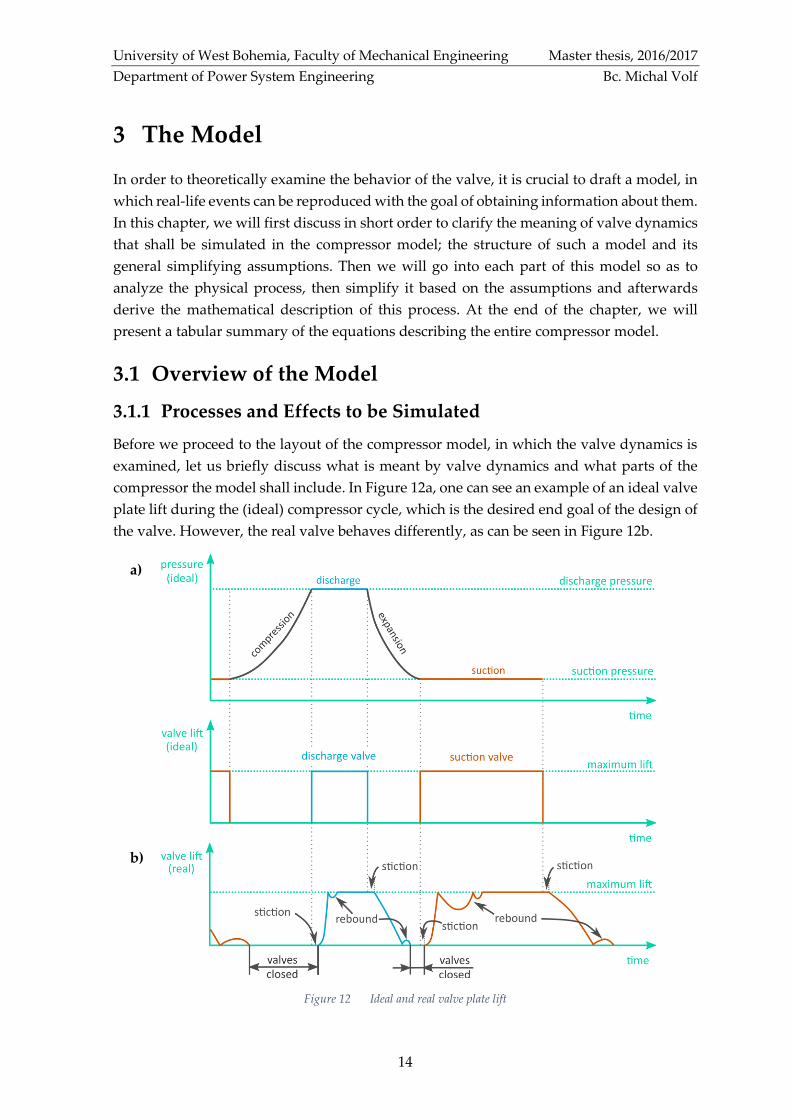
compressor the model shall include. In Figure 12a, one can see an example of an ideal valve
plate lift during the (ideal) compressor cycle, which is the desired end goal of the design of
the valve. However, the real valve behaves differently, as can be seen in Figure 12b.
Figure 12 Ideal and real valve plate lift
a)
b)

University of West Bohemia, Faculty of Mechanical Engineering Master thesis, 2016/2017
Department of Power System Engineering Bc. Michal Volf
15
From the comparison of the two figures above one can clearly observe a significant
difference lying in the valve plate lift over a period of time, which can be attributed to a
variety of effects of valve dynamics such as rebound or stiction, the former of which occurs
when the valve plate strikes against the guard or the limiter, the latter case is the cause of
delayed valve opening or closing. Among the most notable phenomena one should include
the pressure pulsations in the piping system as well as the change in pressure in the
cylinder. Since this thesis is devoted to automatic compressor valves, the latter two can
significantly influence the valve plate lift.
When one is to go about studying valve dynamics, i.e. the motion of the valve plate under
the action of external forces, these effects need to be considered in order to arrive at a valve
design with ideal behavior. It follows that the valve plate lift is the essential quantity when
evaluating valve dynamics.
Regarding the desired output quantities, we can distinguish time-dependent quantities and
so called “periodical” quantities, which contain information about the whole compression
cycle. Included in the former are the valve plate lift, its velocity, pressure in the cylinder,
etc. It is important to note that these variables are strictly required from the perspective of
valve designer [17]. Regarding the latter, i.e. the periodical quantities, examples are
volumetric efficiency, indicated work etc., however, these quantities are not granted much
attention in this thesis, as in addition to the effects of valve dynamics, processes such as
heat transfer through the cylinder wall etc. can also influence them. Since these processes,
discussed individually in relevant chapters, do not considerably influence valve dynamics,
they are not covered in the compressor model and so the accuracy of the periodical results
would be subject to debate.
3.1.2 The Model Structure
In view of the fact that the reciprocating compressor is composed of distinct components,
e.g. a cylinder, a crank mechanism, a suction or discharge system etc., there is no reason to
treat the developed model in a different way. Thus, the drafted model (Figure 13) consists
of several components interacting with each other. The first essential element is a cylinder,
within which the piston moves in a repetitive back-and-forth linear motion. The piston is
driven by a crank mechanism and that as a whole constitutes the second element of the
model. The third and fourth components respectively are formed by the suction and
discharge spring loaded valve, the model of which has already been drafted in chapter 2.3.
The last two elements of the model, are the suction and discharge system of similar
structure.
This model configuration, in which the valve dynamics is examined, is known as the
complete model and it allows for the extensive analysis of the aspects influencing valve
motion since it includes all the components that a real-life reciprocating compressor is
composed of.

University of West Bohemia, Faculty of Mechanical Engineering Master thesis, 2016/2017
Department of Power System Engineering Bc. Michal Volf
16
According to the part of the compressor that is neglected in the model, one can distinguish
three other compressor models; the pipeless model, the valveless model and the
pipe-and-valveless model. The former model, as its name suggests, assumes that the
influence of the suction and discharge piping systems on valve behavior is insignificant and
thus they can be omitted. This model is extensively utilized in literature concerning the
valve dynamics. However, it was found from the experiments carried out by Maclaren [20]
that such a simplification can be considered as invalid since the influence of the piping
system on the valve dynamics can be considerable.
It is evident that the latter two models cannot be used for examining the valve dynamics
since the valves are completely omitted in these models. The valveless model is used
primarily for the investigation of pressure pulsations in the piping system connected to the
piston compressor. Although the pipe-and-valveless model is significantly simplified since
it does not take either the valves or the piping system into account, it finds its use in the
prediction of forces acting on the piston and thus the load of the whole crank mechanism.
The approach to the modular structure of the proposed model and its subsequent
implementation, also allows us to fulfill one of the goals stated in the Purpose of Research,
particularly the one that stated to build a versatile model that can be further adjusted and
easily broadened by others, for instance when the heat transfer through the cylinder wall is
not to be omitted (heat transfer will be neglected in this thesis) etc. This can be simply done
by modifying the mathematical description of one or more of the modules, of which the
compressor model is composed of.
Figure 13 Compressor model
University of West Bohemia, Faculty of Mechanical Engineering Master thesis, 2016/2017
Department of Power System Engineering Bc. Michal Volf
17
3.1.3 Simplifying Assumptions
In the previous section, the workings of the valve dynamics were explained, the general
requirements of the compressor model were discussed and its overall structure was drafted.
In the upcoming subchapters, the processes and effects will be described mathematically
and it would be prudent to introduce some simplifying assumptions for this purpose. Based
on these assumptions, a mathematical model can be derived from the physical one.
Although according to literature pertaining to this topic these two models are commonly
divided into two separate chapters, due to the drafted modular structure of the compressor
model, we believe that this approach would be antithetical to the clarity and readability of
this thesis. Instead, we will discuss each part of the model individually with its physical
processes and subsequent simplifications. In this subchapter, we will elucidate the most
significant simplifying assumptions as well as, wherever possible, their influence on the
accuracy of the results, namely in cases where we have:
• A compressor with one single-acting cylinder
• Rigid bodies
• An ideal gas as the working fluid
• Spring-loaded valves with one degree of freedom
• 1D, quasi-steady subsonic flow
• No reverse flow
The compressor model drafted above, is based on a single stage reciprocating compressor
with one single-acting cylinder. Each part of the compressor, i.e. the cylinder, the piston,
the connecting rod etc. is assumed to be a rigid body and thus the deformations of
compressor elements are not considered. This simplification is made strictly for
completeness; however, its influence on the results can be reckoned as truly negligible.
The working fluid is assumed to be an ideal gas with a constant specific heat capacity. This
simplification was made because it allows us to eliminate in an analytical way several
time-dependent variables, e.g. enthalpy, internal energy etc., which would have required,
had we had a case of a real gas as the working fluid, the use of numerical (iterative)
methods. It follows that this assumption gives us the possibility to substantially simplify
the relevant thermodynamic equations; however, for high pressures real gases do not
strictly follow the ideal gas law and thus this simplification can affect the accuracy of the
results. To illustrate how high the deviation from ideal behavior can be, we make use of a
compressibility factor, which is defined in literature [21]. Assuming piston compressor
parameters, the discharge pressure being up to 150 𝑏𝑎𝑟 and the temperature between
250 − 500 𝐾, the corresponding compressibility factor ranges from 0.94 to 1.065 [22] and
thus the systematic error produced by this simplifying assumption lies within the range of
±6.5 %. Even though, this error is not negligible, it mainly influences the periodic results,
namely the indicated work. Regarding strictly the valve dynamics, Costagliola [9] suggests

University of West Bohemia, Faculty of Mechanical Engineering Master thesis, 2016/2017
Department of Power System Engineering Bc. Michal Volf
18
that there could be some influence in particular to the points of the valve opening or closing,
however, these effects are subtle.
The valves in the compressor model are assumed to be spring-loaded with one degree of
freedom. Although this assumption is not directly linked to the error in the results, it does
not allow us to study the marginal but still somewhat interesting behavior of the valve
plate, e.g. nonparallel collisions etc., which can occur under specific operating
conditions [5].
The penultimate simplification is related to the fluid flow through the valve ports, which
is, in the real compressor, unsteady at least with respect to time. One should bear in mind
that in this thesis, the flow is treated as quasi-steady, i.e. being steady at a given time step
and changing without delay to a new value in the following time-step. This approach is
justified for valves with short channels since in this case delays in valve dynamics, due to
the inertia of the gas resident in the valve channel, will presumably be insignificant [5]. For
the sake of completeness, it is expected that the flow will remain subsonic, i.e. the Mach
number will remain below 1.
Last but not least, if a valve closes late, there can be (for a certain small period of time) a
situation, when the fluid flows in the opposite direction to its regular state, e.g. it is common
that gas flows from the suction chamber into the cylinder; however, there can be a situation,
where the pressure in the cylinder would have to surpass the pressure in the suction
chamber so that the suction valve plate can seal up the valve port - and this is the moment,
when reverse flow can occur. In this thesis, this problem is not discussed since there is
evidence (see [12]) suggesting that it affects the periodical quantities rather than the valve
dynamics.
3.2 Crank Mechanism
The crank mechanism, which is schematically depicted in Figure 14, comprises of a piston,
which is connected via a connecting rod to the crankshaft. Since the piston forms the
movable wall of the cylinder, it is necessary to know its position in calculating the cylinder
volume and thus to determine the thermodynamic process inside. The derivation of this
equation is later presented in this chapter.
Figure 14 Schematic drawing of the crank mechanism
University of West Bohemia, Faculty of Mechanical Engineering Master thesis, 2016/2017
Department of Power System Engineering Bc. Michal Volf
19
To formulate the equation of the instantaneous piston position, assume a set of generalized
coordinates, as follows:
�⃗� = [𝑧, 𝜓, 𝜙]𝑇 (3.2.1)
These coordinates define the position of each moving body with respect to a nonmoving
Cartesian coordinate system, in which the y-axis is identified with the steady front wall of
the cylinder. The positive senses of these coordinates are defined by Figure 14.
Since the crank mechanism has one degree of freedom, only one of these coordinates can
be independent. Let the 𝜙 coordinate be the independent one and then the remaining two
coordinates can be expressed as a function of 𝜙 . For this purpose, two loop equations
relating the three coordinates can be written as:
𝑧 = 𝑧0 + 𝐿 + 𝑅 − 𝐿 cos 𝜓 − 𝑅 cos 𝜙 (3.2.2)
𝐿 sin 𝜓 = 𝑅 sin 𝜙 (3.2.3)
where 𝐿 stands for the connecting rod length, 𝑅 denotes the crank radius and 𝑧0 identifies
the smallest distance between the cylinder and the piston, which is derived from the
clearance volume.
Making use of the Pythagorean identity for the angle 𝜓 , it follows that
Eq. 3.2.3 can be rewritten as:
cos 𝜓 =1
𝐿√𝐿2 − 𝑅2 sin2 𝜙 (3.2.4)
Substituting Eq. 3.2.4 into 3.2.2, we get the piston displacement 𝑧 as a function of the crank
angle 𝜙:
𝑧 = 𝑧0 + 𝐿 + 𝑅 − √𝐿2 − 𝑅2 sin2 𝜙 − 𝑅 cos 𝜙 (3.2.5)
By substituting the crank angle 𝜙 with the following equation
𝜙 = 𝜔𝑡 (3.2.6)
where 𝜔 is the angular velocity of the crankshaft, into the Eq. 3.2.5, we obtain the piston
displacement as only a function of time, since 𝜔 is assumed to be constant:
𝑧 = 𝑧0 + 𝐿 + 𝑅 − √𝐿2 − 𝑅2 sin2(𝜔𝑡) − 𝑅 cos(𝜔𝑡) (3.2.7)
By the differentiation in time of Eq. 3.2.7, one can get the piston velocity 𝑤𝑧 as follows:
𝑤𝑧 = 𝑅 𝜔 sin(𝜔𝑡) (1 +𝑅 cos(𝜔𝑡)
√𝐿2 − 𝑅2 sin2(𝜔𝑡)) (3.2.8)

University of West Bohemia, Faculty of Mechanical Engineering Master thesis, 2016/2017
Department of Power System Engineering Bc. Michal Volf
20
3.3 Cylinder
The physical idea of the process, which takes place inside the cylinder, is rather
straightforward. During the suction phase, when the suction valve is opened, the gas flows
into the cylinder, where it is trapped after both valves are closed and thus the compression
phase takes place. During this process, the pressure of the gas inside the cylinder, as well
as its temperature, rises due to the reduction of the cylinder volume. Moreover, heat
transfer through the cylinder walls and the piston is also present. Initially, when the
temperature of the gas is lower than the temperature of the walls, the temperature of the
gas will rise; however, should its temperature increase such, so that it is higher than that of
the wall’s, the heat transfer will take place the other way around and thus the gas will start
to be cooled. If the pressure in the cylinder reaches sufficiently high values, the discharge
valve plate will be pushed away and the compressed gas will be forced out of cylinder.
Finally, when both of the valves are closed again, the pressure inside the cylinder decreases
due to the expansion of the remaining compressed gas in the clearance volume.
3.3.1 Simplifying assumptions
To arrive at a mathematical description of the process outlined above, lets discuss the
assumptions which are taken into consideration here:
• No gas leakage
• The kinetic and potential energy of the gas is neglected
• Homogenous system
• Adiabatic control volume
If either the valve plates or piston rod packings, are subject to a certain degree of wear, the
gas inside the cylinder can leak. Nevertheless, in the derivations of the mathematical
equations in the following sections, these leaks are not considered and thus it is assumed
that the change of mass inside the cylinder is only caused by the gas flow through the valves
during either the suction or the discharge phase.
The second simplification, i.e. neglecting both the kinetic and potential energy, is valid for
the gas inside the cylinder and the suction/discharge chambers as well as for the gas
entering or leaving it. Although the reason to neglect the potential energy is obvious since
there are not any appreciable height differences, neglecting the kinetic energy requires
careful deliberation. Regarding the gas flowing through the valves, it can be freely stated
that despite the rather high velocity of the gas in a valve port, the kinetic energy is irrelevant
if the control volume is chosen in such a way that its boundaries are out of the valve port.
To vindicate the neglecting of kinetic energy of the gas in the cylinder or suction/discharge
chamber, assume an adiabatic compression (pressure ratio equal to three) of air (20 °C). The
compression work would be approximately 75000 J/kg. This is far more than the kinetic
energy, because even in cases where the air would be accelerated from at rest to a velocity
of 20 m/s, the kinetic energy would be only about 200 J/kg.

University of West Bohemia, Faculty of Mechanical Engineering Master thesis, 2016/2017
Department of Power System Engineering Bc. Michal Volf
21
The cylinder volume is considered as a homogenous thermodynamic system, in which the
physical properties are the same in all parts of the system. Despite there being evidence of
changes in properties from one point to another [23], this assumption is requisite so that the
energy distribution in the system is known and thus it is feasible to theoretically
calculate it.
Despite the fact that the last simplification, i.e. not taking into account the heat transfer
through both the cylinder walls and the piston, does influence the predicted compressor
performance, e.g. its efficiency and indicated work, it does not significantly influence the
valve dynamics [12] and thus it will be assumed.
3.3.2 General Governing Equations
In this subchapter, we present the derivation of the equation, which describes the change
of the state of the gas inside the cylinder. For this purpose, we utilize the conservation of
energy principle, which in its most general form states that the time rate change of energy
inside the control volume is equal to the rate of net energy transfer. According to
literature [24], this can be expressed as:
𝑑𝐸𝐶𝑉
𝑑𝑡= lim
𝑑𝑡→0(
𝛿𝐸𝑖𝑛
𝑑𝑡) − lim
𝑑𝑡→0(
𝛿𝐸𝑜𝑢𝑡
𝑑𝑡) = �̇�𝑖𝑛 − �̇�𝑜𝑢𝑡 (3.3.1)
where 𝐸𝐶𝑉 identifies the energy of gas inside the control volume, �̇�𝑖𝑛,𝑜𝑢𝑡 is the rate of energy
flowing into or out of the control volume.
According to Gramoll [25], the energy can be transferred by heat, work and mass only, and
thus the energy balance can then be rewritten as:
𝑑𝐸𝐶𝑉
𝑑𝑡= �̇� − �̇� + ∑ �̇�𝑖𝑛𝑒𝑖𝑛 − ∑ �̇�𝑜𝑢𝑡𝑒𝑜𝑢𝑡 (3.3.2)
where �̇� stands for the rate of total heat transfer to the system, �̇� is the rate of total work
done by the system and 𝑒𝑖𝑛,𝑜𝑢𝑡 represents the total energy carried by a unit of mass as it
enters or leaves the control volume (see Eq. 3.3.3).
𝑒 =𝑤2
2+ 𝑔𝑦 + 𝑢 + 𝑝𝑣 =
𝑤2
2+ 𝑔𝑦 + ℎ (3.3.3)
where 𝑤2
2 is the kinetic energy, 𝑔𝑦 represents the potential energy,
𝑢 stands for the internal energy and 𝑝𝑣 denotes the flow work. It is important to note that
all of the terms are specific (i.e. per mass unit). Together the latter two terms form the
specific enthalpy ℎ. It shall be emphasized that the specific energy of gas inside the control
volume can also be calculated as per Eq. 3.3.3, however, omitting the additional energy in
the form of flow work.
University of West Bohemia, Faculty of Mechanical Engineering Master thesis, 2016/2017
Department of Power System Engineering Bc. Michal Volf
22
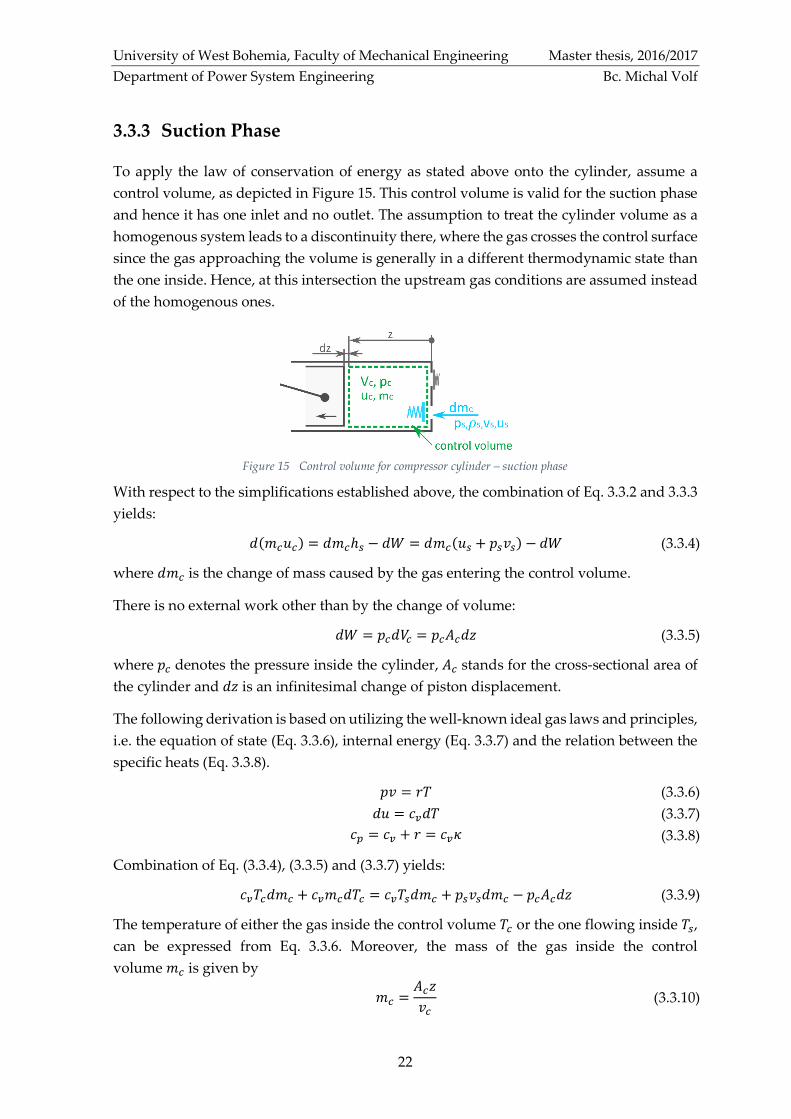
3.3.3 Suction Phase
To apply the law of conservation of energy as stated above onto the cylinder, assume a
control volume, as depicted in Figure 15. This control volume is valid for the suction phase
and hence it has one inlet and no outlet. The assumption to treat the cylinder volume as a
homogenous system leads to a discontinuity there, where the gas crosses the control surface
since the gas approaching the volume is generally in a different thermodynamic state than
the one inside. Hence, at this intersection the upstream gas conditions are assumed instead
of the homogenous ones.
With respect to the simplifications established above, the combination of Eq. 3.3.2 and 3.3.3
yields:
𝑑(𝑚𝑐𝑢𝑐) = 𝑑𝑚𝑐ℎ𝑠 − 𝑑𝑊 = 𝑑𝑚𝑐(𝑢𝑠 + 𝑝𝑠𝑣𝑠) − 𝑑𝑊 (3.3.4)
where 𝑑𝑚𝑐 is the change of mass caused by the gas entering the control volume.
There is no external work other than by the change of volume:
𝑑𝑊 = 𝑝𝑐𝑑𝑉𝑐 = 𝑝𝑐𝐴𝑐𝑑𝑧 (3.3.5)
where 𝑝𝑐 denotes the pressure inside the cylinder, 𝐴𝑐 stands for the cross-sectional area of
the cylinder and 𝑑𝑧 is an infinitesimal change of piston displacement.
The following derivation is based on utilizing the well-known ideal gas laws and principles,
i.e. the equation of state (Eq. 3.3.6), internal energy (Eq. 3.3.7) and the relation between the
specific heats (Eq. 3.3.8).
𝑝𝑣 = 𝑟𝑇 (3.3.6)
𝑑𝑢 = 𝑐𝑣𝑑𝑇 (3.3.7)
𝑐𝑝 = 𝑐𝑣 + 𝑟 = 𝑐𝑣𝜅 (3.3.8)
Combination of Eq. (3.3.4), (3.3.5) and (3.3.7) yields:
𝑐𝑣𝑇𝑐𝑑𝑚𝑐 + 𝑐𝑣𝑚𝑐𝑑𝑇𝑐 = 𝑐𝑣𝑇𝑠𝑑𝑚𝑐 + 𝑝𝑠𝑣𝑠𝑑𝑚𝑐 − 𝑝𝑐𝐴𝑐𝑑𝑧 (3.3.9)
The temperature of either the gas inside the control volume 𝑇𝑐 or the one flowing inside 𝑇𝑠,
can be expressed from Eq. 3.3.6. Moreover, the mass of the gas inside the control
volume 𝑚𝑐 is given by
𝑚𝑐 =𝐴𝑐𝑧
𝑣𝑐 (3.3.10)
Figure 15 Control volume for compressor cylinder – suction phase
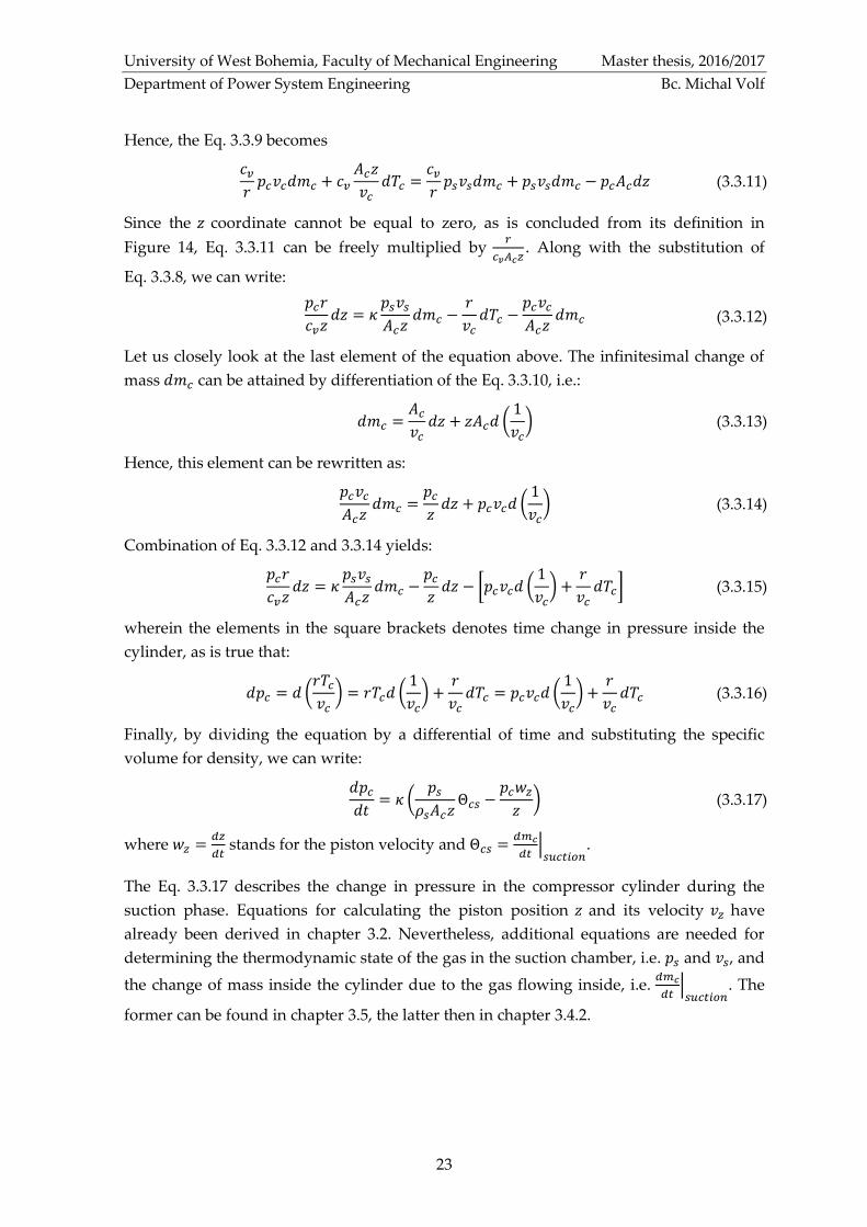
University of West Bohemia, Faculty of Mechanical Engineering Master thesis, 2016/2017
Department of Power System Engineering Bc. Michal Volf
23
Hence, the Eq. 3.3.9 becomes
𝑐𝑣
𝑟𝑝𝑐𝑣𝑐𝑑𝑚𝑐 + 𝑐𝑣
𝐴𝑐𝑧
𝑣𝑐𝑑𝑇𝑐 =
𝑐𝑣
𝑟𝑝𝑠𝑣𝑠𝑑𝑚𝑐 + 𝑝𝑠𝑣𝑠𝑑𝑚𝑐 − 𝑝𝑐𝐴𝑐𝑑𝑧 (3.3.11)
Since the 𝑧 coordinate cannot be equal to zero, as is concluded from its definition in
Figure 14, Eq. 3.3.11 can be freely multiplied by 𝑟
𝑐𝑣𝐴𝑐𝑧. Along with the substitution of
Eq. 3.3.8, we can write:
𝑝𝑐𝑟
𝑐𝑣𝑧𝑑𝑧 = 𝜅
𝑝𝑠𝑣𝑠
𝐴𝑐𝑧𝑑𝑚𝑐 −
𝑟
𝑣𝑐𝑑𝑇𝑐 −
𝑝𝑐𝑣𝑐
𝐴𝑐𝑧𝑑𝑚𝑐 (3.3.12)
Let us closely look at the last element of the equation above. The infinitesimal change of
mass 𝑑𝑚𝑐 can be attained by differentiation of the Eq. 3.3.10, i.e.:
𝑑𝑚𝑐 =𝐴𝑐
𝑣𝑐𝑑𝑧 + 𝑧𝐴𝑐𝑑 (
1
𝑣𝑐) (3.3.13)
Hence, this element can be rewritten as:
𝑝𝑐𝑣𝑐
𝐴𝑐𝑧𝑑𝑚𝑐 =
𝑝𝑐
𝑧𝑑𝑧 + 𝑝𝑐𝑣𝑐𝑑 (
1
𝑣𝑐) (3.3.14)
Combination of Eq. 3.3.12 and 3.3.14 yields:
𝑝𝑐𝑟
𝑐𝑣𝑧𝑑𝑧 = 𝜅
𝑝𝑠𝑣𝑠
𝐴𝑐𝑧𝑑𝑚𝑐 −
𝑝𝑐
𝑧𝑑𝑧 − [𝑝𝑐𝑣𝑐𝑑 (
1
𝑣𝑐) +
𝑟
𝑣𝑐𝑑𝑇𝑐] (3.3.15)
wherein the elements in the square brackets denotes time change in pressure inside the
cylinder, as is true that:
𝑑𝑝𝑐 = 𝑑 (𝑟𝑇𝑐
𝑣𝑐) = 𝑟𝑇𝑐𝑑 (
1
𝑣𝑐) +
𝑟
𝑣𝑐𝑑𝑇𝑐 = 𝑝𝑐𝑣𝑐𝑑 (
1
𝑣𝑐) +
𝑟
𝑣𝑐𝑑𝑇𝑐 (3.3.16)
Finally, by dividing the equation by a differential of time and substituting the specific
volume for density, we can write:
𝑑𝑝𝑐
𝑑𝑡= 𝜅 (
𝑝𝑠
𝜌𝑠𝐴𝑐𝑧Θ𝑐𝑠 −
𝑝𝑐𝑤𝑧
𝑧) (3.3.17)
where 𝑤𝑧 =𝑑𝑧
𝑑𝑡 stands for the piston velocity and Θ𝑐𝑠 =
𝑑𝑚𝑐
𝑑𝑡|
𝑠𝑢𝑐𝑡𝑖𝑜𝑛.
The Eq. 3.3.17 describes the change in pressure in the compressor cylinder during the
suction phase. Equations for calculating the piston position 𝑧 and its velocity 𝑣𝑧 have
already been derived in chapter 3.2. Nevertheless, additional equations are needed for
determining the thermodynamic state of the gas in the suction chamber, i.e. 𝑝𝑠 and 𝑣𝑠, and
the change of mass inside the cylinder due to the gas flowing inside, i.e. 𝑑𝑚𝑐
𝑑𝑡|
𝑠𝑢𝑐𝑡𝑖𝑜𝑛. The
former can be found in chapter 3.5, the latter then in chapter 3.4.2.
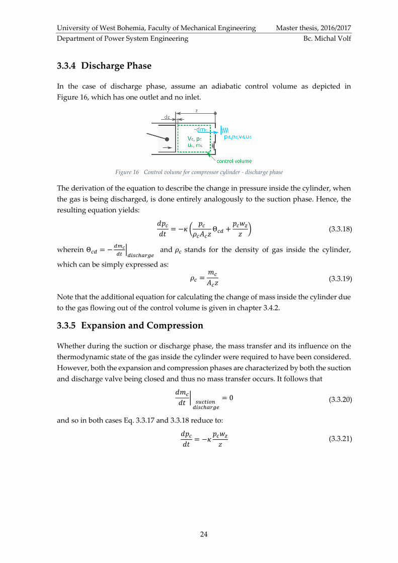
University of West Bohemia, Faculty of Mechanical Engineering Master thesis, 2016/2017
Department of Power System Engineering Bc. Michal Volf
24
3.3.4 Discharge Phase
In the case of discharge phase, assume an adiabatic control volume as depicted in
Figure 16, which has one outlet and no inlet.
The derivation of the equation to describe the change in pressure inside the cylinder, when
the gas is being discharged, is done entirely analogously to the suction phase. Hence, the
resulting equation yields:
𝑑𝑝𝑐
𝑑𝑡= −𝜅 (
𝑝𝑐
𝜌𝑐𝐴𝑐𝑧Θ𝑐𝑑 +
𝑝𝑐𝑤𝑧
𝑧) (3.3.18)
wherein Θ𝑐𝑑 = −𝑑𝑚𝑐
𝑑𝑡|𝑑𝑖𝑠𝑐ℎ𝑎𝑟𝑔𝑒
and 𝜌𝑐 stands for the density of gas inside the cylinder,
which can be simply expressed as:
𝜌𝑐 =𝑚𝑐
𝐴𝑐𝑧 (3.3.19)
Note that the additional equation for calculating the change of mass inside the cylinder due
to the gas flowing out of the control volume is given in chapter 3.4.2.
3.3.5 Expansion and Compression
Whether during the suction or discharge phase, the mass transfer and its influence on the
thermodynamic state of the gas inside the cylinder were required to have been considered.
However, both the expansion and compression phases are characterized by both the suction
and discharge valve being closed and thus no mass transfer occurs. It follows that
𝑑𝑚𝑐
𝑑𝑡|
𝑠𝑢𝑐𝑡𝑖𝑜𝑛 𝑑𝑖𝑠𝑐ℎ𝑎𝑟𝑔𝑒
= 0 (3.3.20)
and so in both cases Eq. 3.3.17 and 3.3.18 reduce to:
𝑑𝑝𝑐
𝑑𝑡= −𝜅
𝑝𝑐𝑤𝑧
𝑧 (3.3.21)
Figure 16 Control volume for compressor cylinder - discharge phase

University of West Bohemia, Faculty of Mechanical Engineering Master thesis, 2016/2017
Department of Power System Engineering Bc. Michal Volf
25
3.4 Suction and Discharge Valve
In this chapter, we intend to present the mathematical description of the valve behavior.
First, we present the equation describing the gas flow through the valve as a function of
time or rather of the valve plate lift, which is truly the sine qua non-of linking the
thermodynamic state of gas in the cylinder to the one present in suction or discharge
chamber. Second, the force balance on valve plate lift is drawn up in order to predict the
valve plate motion.
One should bear in mind that since the mathematical description is fundamentally the same
for both the suction and discharge valve, this section refers to both simultaneously. Hence,
some changes in the pressure notation are made:
• Pressure 𝑝𝑢 denotes the pressure in front of the valve (in respect to the normal gas
flow), i.e. for the suction valve it corresponds to the pressure in the suction
chamber 𝑝𝑠 , whereas for the discharge valve it refers to the pressure in
the cylinder 𝑝𝑐
• Pressure 𝑝𝑑 stands for the pressure behind the valve, i.e. for the suction valve it
refers to the pressure in the cylinder 𝑝𝑐, for the discharge valve it corresponds to the
pressure in the discharge chamber 𝑝𝑑
3.4.1 Simplifying assumptions
Regarding the simplifying assumptions that take place in terms of valve modeling, most of
them has already been discussed, namely:
• Spring-loaded rigid body with one degree of freedom (valve plate can only move in
the direction perpendicular to the plane of the seat)
• Quasi-steady flow
• Ideal gas
• No reverse flow
Moreover, another remark is needed particularly in relation to the transition of the real
compressor valve to the model one. Up to now, it has been tacitly assumed that the
reciprocating compressor or rather the model of it, in which the valve dynamics is
examined, has solely one suction and one discharge valve; a design that there is only one
valve port in each valve through which the gas flows. However, in real-life compressor
valves (discussed in chapter 2.2) there are usually many ports. Moreover, the compressor
can be equipped with more than one suction and discharge valve. Customarily in these
cases [12], the valve model may be based either on the concept of one larger replacement
valve or many small valves, however with the same properties. In this thesis, it is assumed
that the former approach is utilized.
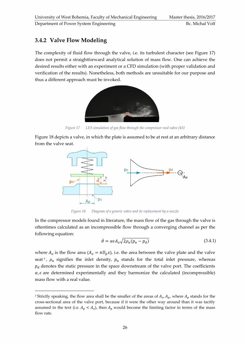
University of West Bohemia, Faculty of Mechanical Engineering Master thesis, 2016/2017
Department of Power System Engineering Bc. Michal Volf
26
3.4.2 Valve Flow Modeling
The complexity of fluid flow through the valve, i.e. its turbulent character (see Figure 17)
does not permit a straightforward analytical solution of mass flow. One can achieve the
desired results either with an experiment or a CFD simulation (with proper validation and
verification of the results). Nonetheless, both methods are unsuitable for our purpose and
thus a different approach must be invoked.
Figure 18 depicts a valve, in which the plate is assumed to be at rest at an arbitrary distance
from the valve seat.
In the compressor models found in literature, the mass flow of the gas through the valve is
oftentimes calculated as an incompressible flow through a converging channel as per the
following equation:
�̇� = 𝛼𝜖𝐴𝑜√2𝜌𝑢(𝑝𝑢 − 𝑝𝑑) (3.4.1)
where 𝐴𝑜 is the flow area (𝐴𝑜 = 𝜋𝐷𝑝𝑥), i.e. the area between the valve plate and the valve
seat 3 , 𝜌𝑢 signifies the inlet density, 𝑝𝑢 stands for the total inlet pressure, whereas
𝑝𝑑 denotes the static pressure in the space downstream of the valve port. The coefficients
𝛼, 𝜖 are determined experimentally and they harmonize the calculated (incompressible)
mass flow with a real value.
3 Strictly speaking, the flow area shall be the smaller of the areas of 𝐴𝑜, 𝐴𝑝, where 𝐴𝑝 stands for the
cross-sectional area of the valve port, because if it were the other way around than it was tacitly
assumed in the text (i.e. 𝐴𝑝 < 𝐴𝑜), then 𝐴𝑝 would become the limiting factor in terms of the mass
flow rate.
Figure 17 LES simulation of gas flow through the compressor reed valve [43]
Figure 18 Diagram of a generic valve and its replacement by a nozzle

University of West Bohemia, Faculty of Mechanical Engineering Master thesis, 2016/2017
Department of Power System Engineering Bc. Michal Volf
27
According to corresponding literature [5] it is stated that the former, so-called flow coefficient
𝛼, accounts for the influence of viscosity, the vena contracta after flow separation and the
non-uniform state of gas in the cross-sections perpendicular to the flow direction. Since
from completed experiments [12] it can be seen that the values of the flow coefficient are
below 1, i.e. the predicted mass flow rate is higher than the real one, we feel that it could be
questionable if the lower mass flow rate was purely due to the above stated reasons or
rather due to the irreversibility in throttling flow (i.e. generating entropy). Moreover, the
experiments showed that the value of the coefficient almost entirely depends on the
geometrical shape of the flow passage (and thus of the valve plate lift) instead of either
operating conditions or the size of the valve.
The second coefficient, i.e. the so-called expansion coefficient 𝜖, allows for the compressibility
of the gas. However, in this case, experiments [12] proved that its value is not a function of
purely pressure ratio across the valve, but also of the valve geometry, its size as well as the
properties of the gas.
In this thesis, we will avoid utilizing the expansion coefficient due to the variety of factors
influencing it, by modeling the fluid flow as the outflow of gas from a pressurized vessel
through a convergent nozzle by assuming isentropic expansion between the upstream and
downstream conditions. In cases with ideal gas, it can be calculated by invoking the
well-known Saint-Venant-Wantzel equation:
�̇� = 𝛼𝐴𝑜√2𝜅
𝜅 − 1𝑝𝑢𝜌𝑢 ((
𝑝𝑑
𝑝𝑢)
2𝜅
− (𝑝𝑑
𝑝𝑢)
𝜅+1𝜅
) (3.4.2)
wherein the flow coefficient is used to account for the irreversibility of the process. One
should bear in mind that if the pressure ratio in Eq. 3.4.2 is equal to the critical pressure
ratio
𝑝𝑑
𝑝𝑢= (
2
𝜅 + 1)
𝜅𝜅−1
= 0.528|𝜅=1.4 (3.4.3)
the valve will become choked and thus Eq. 3.4.2 cannot be used as a mass flow rate model.
However, Ninković [2], based on Böswirth’s findings, states that compressor valves do not
become choked in accordance to Eq. 3.4.3, yet they do at much higher-pressure ratios;
hence, beyond the critical pressure ratio, the necessitation of undergoing an experiment or
a CFD simulation is inevitable in order to arrive at a mass flow rate.
By substituting the flow area into Eq. 3.4.2, we get:
Θ̇ = 𝛼𝜋𝐷𝑝𝑥√2𝜅
𝜅 − 1𝑝𝑢𝜌𝑢 ((
𝑝𝑑
𝑝𝑢)
2𝜅
− (𝑝𝑑
𝑝𝑢)
𝜅+1𝜅
) (3.4.4)

University of West Bohemia, Faculty of Mechanical Engineering Master thesis, 2016/2017
Department of Power System Engineering Bc. Michal Volf
28
By noticing that by comparing Eqs. 3.4.1 and 3.4.2, one can arrive at a means, by which the
expansion coefficient can be theoretically determined as follows:
𝜖 = √𝜅
𝜅 − 1
𝑝𝑢
𝑝𝑢 − 𝑝𝑑 ((
𝑝𝑑
𝑝𝑢)
2𝜅
− (𝑝𝑑
𝑝𝑢)
𝜅+1𝜅
) (3.4.5)
This can be considered a basic approach to determine the expansion coefficient, since one
can find other more sophisticated ways to theoretically determine 𝜖 in literature [26], which
found its use, for instance, in those cases where strong contractions take place etc.
3.4.3 Valve Dynamics
As already stated, the movable valve plate is considered to be a mass-spring system with a
single degree of freedom (Figure 19). Hence, the equation of motion is based on Newton’s
second law:
𝑚𝑑2𝑥
𝑑𝑡2+ 𝐹𝑓 + 𝐹𝑠 = 𝐹𝑔 (3.4.6)
where 𝑚 is the mass in motion, 𝑥 stands for the distance of the valve plate from the seat,
𝐹𝑔 stands for the gas force, 𝐹𝑓 denotes the fluid friction force and 𝐹𝑠 indicates the spring
force. If the valve plate reaches an obstacle (a seat or limiter), a rebound can occur.
Afterwards, the plate comes into direct contact with the obstacle, accompanied with the
appearance of an adhesion force 𝐹𝑎𝑑ℎ.
Before proceeding to the analysis of these quantities individually, let us look at the force
balances for the valve plate, when it is at rest, i.e. when it is in contact with the limiter or
the seat, and what conditions must be fulfilled so that its movement is enforced again.
Valve in Closed State
If the valve is closed, then the following inequation is fulfilled:
𝑝𝑢𝐴𝑝 − 𝑝𝑑𝐴𝑣 ≤ 𝐹𝑠 + 𝐹𝑎𝑑ℎ (3.4.7)
When this inequality condition reverses, the valve plate will lift, i.e.:
𝑝𝑢𝐴𝑝 − 𝑝𝑑𝐴𝑣 > 𝐹𝑠 + 𝐹𝑎𝑑ℎ (3.4.8)
Figure 19 Force balance on valve plate

University of West Bohemia, Faculty of Mechanical Engineering Master thesis, 2016/2017
Department of Power System Engineering Bc. Michal Volf
29
Valve in Fully Open State
If the sum of the forces pushing the valve plate towards the limiter is higher than the spring
force acting in the opposite direction, then the valve plate will remain in a fully open state,
i.e.:
𝐹𝑠 ≤ 𝐹𝑔 + 𝐹𝑎𝑑ℎ (3.4.9)
Analogously to the previous event, when the inequality is not fulfilled anymore, i.e. the
following is true:
𝐹𝑠 > 𝐹𝑔 + 𝐹𝑎𝑑ℎ (3.4.10)
the valve plate will then start to move back towards the valve seat.
3.4.3.1 The Mass of the System
The mass 𝑚 in Eq. 3.4.6 does not refer solely to the mass of the valve plate, but since the
spring generally has a non-negligible mass, it needs to also be included in the term of 𝑚.
Moreover, as the valve plate moves through the fluid, some of the volume of the
surrounding fluid needs to be deflected. This effect can be covered by the so-called added
mass, which can be determined by means of potential flow theory. However, since the
working fluid in the compressor is assumed to be air, its density is much lower in
comparison with the material of the plate and thus the added mass would be considerably
lower than the mass of the plate. It follows that this effect can be neglected.
Regarding the mass of the spring, it cannot be simply added to the mass of the plate, since
the velocity, with which the spring elements move, is proportional to the length of the
spring, i.e. 𝜁
𝑙
𝑑𝑥
𝑑𝑡. Instead, an effective mass needs to be determined. This can be done
theoretically based on the kinetic energy of the spring.
If the kinetic energy 𝑑𝐸𝑘,𝑠𝑝𝑟𝑖𝑛𝑔 of a spring element (with mass 𝑑𝜁
𝑙𝑚𝑠𝑝𝑟𝑖𝑛𝑔 ) is equal to
1
2
𝑑𝜁
𝑙𝑚𝑠𝑝𝑟𝑖𝑛𝑔 (
𝜁
𝑙
𝑑𝑥
𝑑𝑡)
2, the kinetic energy of the whole spring is then:
𝐸𝑘,𝑠𝑝𝑟𝑖𝑛𝑔 = ∫ 𝑑𝐸𝑘,𝑠𝑝𝑟𝑖𝑛𝑔
𝜁=𝑙
𝜁=0
=1
2
𝑚𝑠𝑝𝑟𝑖𝑛𝑔
3(
𝑑𝑥
𝑑𝑡)
2
(3.4.11)
It follows that the inertial effect of the spring can be accounted for by adding one third of
the spring mass to the mass of the valve plate, i.e.:
𝑚 = 𝑚𝑝𝑙𝑎𝑡𝑒 +1
3𝑚𝑠𝑝𝑟𝑖𝑛𝑔 (3.4.12)
Figure 20 Effective spring mass

University of West Bohemia, Faculty of Mechanical Engineering Master thesis, 2016/2017
Department of Power System Engineering Bc. Michal Volf
30
3.4.3.2 Spring Force
The majority of compressor valve springs can be modeled as springs with linear
characteristics (see Figure 21) [9].
In this case, the spring force is given simply by:
𝐹𝑠 = 𝑘(𝑥0 + 𝑥) (3.4.13)
where 𝑘 is the spring stiffness (𝑘 = tan 𝛼) and 𝑥0 stands for the preload deflection.
3.4.3.3 Valve Plate Impacts
As already mentioned, the valve plate is limited in its motion by the valve limiter and the
valve seat. The former limits the motion when the valve plate is lifting, whereas the latter
comes into action when the valve is about to close. When the moving plate strikes against
these fixed obstacles, it will rebound with a velocity that is fundamentally lower than the
one at the moment of impact. In order to avoid the rebound of the valve plate, the kinetic
energy would have to be entirely dissipated (absorbed).
The valve plate impacts are modeled based on Newton’s experimental law, which presents
us with the following equation [27]:
𝑑𝑥
𝑑𝑡|
𝑡+= −𝑐𝑟
𝑑𝑥
𝑑𝑡|
𝑡− (3.4.14)
Where 𝑐𝑟 is the restitution coefficient, 𝑑𝑥
𝑑𝑡|𝑡−
denotes the (relative) velocity just before the
impact, whereas 𝑑𝑥
𝑑𝑡|
𝑡+ stands for the (relative) velocity immediately after the impact.
Obviously, if the restitution coefficient equals zero, no rebound occurs and thus the impact
is referred to as inelastic. On the other hand, should the coefficient be equal to 1, then the
valve plate rebounds with the same velocity as it had at the moment of impact. This kind
of impact is called fully elastic. These are essentially extreme cases, since in reality the
restitution coefficient will typically range from zero to one and thus the impact will be
semi-elastic. Since the impacts give rise to stress concentration, which leads to impact
fatigue, it is evident that a value of zero is desired for the restitution coefficient.
The drawback here is that the knowledge of valve parts’ materials and their elastic
properties is insufficient for a theoretical prediction of the restitution coefficient [5], because
of many more factors involved in. For instance, the classical impact between two solid
bodies is not likely to occur here, since as the valve approaches an obstacle, it has to displace
the gas and the oil in the space between the obstacle and the plate.
Figure 21 Linear spring characteristic

University of West Bohemia, Faculty of Mechanical Engineering Master thesis, 2016/2017
Department of Power System Engineering Bc. Michal Volf
31
Lastly it should be remarked that the influence of valve plate impacts in the mathematical
model is accounted for by the initial conditions needed to solve the system of ODEs. In
other words, the system of ODEs is being solved until the valve plate strikes against a seat
or guard when the system of ODEs will be solved anew; however, the initial velocity of the
valve plate there will be in conformity with Eq. 3.4.14.
3.4.3.4 Friction Force
Assuming the valve plate is in an arbitrary position between the valve seat and the limiter,
but is not touching either of them, then the motion of the valve plate is damped by the fluid
friction opposing the motion of the valve plate. As Ninković [2] points out, this friction force
acting on the moving plate can be assumed to be proportional to the velocity of the
plate, i.e.:
𝐹𝑓 = 𝑐𝑓
𝑑𝑥
𝑑𝑡 (3.4.15)
where 𝑐𝑓 denotes the friction coefficient.
From the experiments done by Touber [12] one can see that the friction coefficient is
basically independent of gas density and thus the same value can be used for both the
suction and discharge valves, if they are of the same design and dimensions. Moreover, but
somewhat surprisingly, his experiments showed a weak dependence of the friction
coefficient on the oil droplets in the gas stream. However, we feel that more experiments
might be desirable to further verify this statement, since the author only states the
percentage of oil in the gas stream, but does not discuss for instance the size of the oil
droplets etc., which could likely influence the results.
3.4.3.5 Adhesion
When the valve is in contact with the limiter or the seat, an adhesion (or sometimes referred
to as stiction) appears. It negatively influences the valve behavior, since the valve will not
start moving immediately after the upstream pressure 𝑝𝑢 exceeds the downstream
pressure 𝑝𝑑 . Nevertheless, a sufficient pressure difference is needed to overcome the
stiction effect. Hence the valve plate starts moving much later than in absence of adhesion.
Strictly speaking, adhesion is present in both lubricated and non-lubricated machines.
However, in the former, the effect is far more noticeable and the situation is much more
complicated, since it is mainly caused by the deformation of a lubricating oil film in the gap
between the valve plate and the obstacle [2]. It follows that the amount of oil, its viscosity
varying with its temperature etc., influences this effect. Many of the compressor models
presented in literature (for example [5] [28]) tacitly assume the latter case and as a
consequence of which they completely omit the stiction effect. In this thesis, the former case
is modeled, i.e. the stiction in the case of a lubricated machine.
The complex nature of the physical background of adhesion in a lubricated machine, which
is beyond the scope of this thesis, gives rise to many models trying to simulate this effect.
However, most of them are semi-empirical. Recently, a study by Pizarro-Recabarren,

University of West Bohemia, Faculty of Mechanical Engineering Master thesis, 2016/2017
Department of Power System Engineering Bc. Michal Volf
32
Barbosa and Deschamps [29] was published, regarding the stiction effect in automatic
compressor valves. They proposed a very extensive model for the prediction of stiction,
departing from the Reynolds equation for hydrodynamic lubrication, in which they
consider effects like oil film rupture etc. However, as they state, experimental work is
needed to validate their model.
In this thesis, we will utilize a different theoretical model proposed by Khalifa and Liu [30],
in which it is assumed that the entire space between the plate and the obstacle (delimited
by 𝐷𝑝 and 𝐷𝑣) is always occupied by oil. Moreover, the change in cross-section of the oil
film preceding its rupture is not considered here. The outcome of this model encompasses
the fact that the rupture of the oil film cannot be predicted and that the effect of stiction can
only be considered when the valve plate is stationary, even though in real-life the adhesion
force ceases to exist at the moment the oil film starts to disrupt, not the moment in which
the valve plate is set in motion.
The oil film stiction force can be expressed as a sum of the force component due to the
viscous effects 𝐹𝑣𝑖𝑠𝑐, the capillary force 𝐹𝑐𝑎𝑝 and the interfacial tension force 𝐹𝑡𝑒𝑛 [29], i.e.:
𝐹𝑎𝑑ℎ = 𝐹𝑣𝑖𝑠𝑐 + 𝐹𝑐𝑎𝑝 + 𝐹𝑡𝑒𝑛 (3.4.16)
In the Khalifa and Liu model [30], no account is made for the liquid-gas interfacial tension,
i.e. 𝐹𝑡𝑒𝑛 = 0. Since the valve plate is stationary, the viscous force (which is proportional to
the velocity of the plate) also vanishes and thus one can get:
𝐹𝑎𝑑ℎ ≡ 𝐹𝑐𝑎𝑝 =𝜋𝛾𝐿𝐺𝐷𝑝
2 cos 𝛽
2ℎ𝑓𝑖𝑙𝑚((
𝐷𝑣
𝐷𝑝)
2
− 1) (3.4.17)
wherein 𝛾𝐿𝐺 stands for surface tension, 𝛽 denotes a meniscus contact angle and ℎ𝑓𝑖𝑙𝑚 refers
to oil film thickness (see Figure 22).
Strictly speaking, Eq. 3.4.17 applies to the contact area between the valve plate and the seat
and thus different areas should be used to arrive at the equation for the adhesion force
between the valve plate and the guard. However, in this thesis Eq. 3.4.17 will be used for
the latter case as well, since we are not in possession of the dimensions of the valve limiter.
Moreover, the stiction effect is accounted for only in cases where the valve plate is pressed
against the obstacle for a finite time. This is in compliance with the fact, that short moments
Figure 22 Stiction
University of West Bohemia, Faculty of Mechanical Engineering Master thesis, 2016/2017
Department of Power System Engineering Bc. Michal Volf
33
of contact, such when the valve plate strikes against the obstacle and rebounds
immediately, do not give rise to a noticeable adhesion effect [30].
3.4.3.6 Fluid-Structure Interaction
In view of the fact that our interest in this thesis is focused on automatic compressor valves;
the essence of predicting the motion of the valve plate lies in the interaction of the fluid
flow with the plate. However, the physical complexity of this interaction, caused by both
the flow and the plate, incurs difficulties if one wants to predict it instead of purely
foreseeing it.
It is reasonable to expect the flow (in a real-life valve) to be turbulent, three-dimensional,
compressible, unsteady, and likely to be a multi-phase flow containing oil particles. The
valve plate can generally be classified as a sharp-edged bluff body immersed in a fluid flow
field, which it resists. Hence, the fluid flow exerts the force acting on the body, which
originates from the uneven pressure distribution around the valve plate. If the pressure
distribution was known, this force could be easily calculated as a surface integral of the
pressure around the valve plate. Unfortunately, this is not happening here.
As Habing [5] states, even in cases with incompressible flow, the force acting on the body
immersed in a fluid flow field could generally be expressed in only two exceptional cases;
either for a steady viscous creeping flow (𝑅𝑒 ≪ 1) or for an irrotational inviscid unsteady
flow. However, the same author also concludes that neither of these two approaches is
applicable for compressor valves.
Hence, the gas force exerted on the valve plate will be modeled as the force acting on the
plate in quasi-steady flow, i.e.:
𝐹𝑔 = 𝑐𝑔𝐴𝑣(𝑝𝑢 − 𝑝𝑑) (3.4.18)
whereby 𝐴𝑣 denotes the valve plate area and 𝑐𝑔 stands for the gas force coefficient4, which
is a function of the valve plate lift, i.e. 𝑐𝑔(𝑥) . This method of calculating gas force is
customarily employed in corresponding literature (for instance see [5] [12] [2] [31]), since it
is widely recognized as a workable definition.
The values of the gas coefficient are subject to the experiment, which requires the use of a
dynamometer attached to the valve plate. Experimental data for various valve designs can
be found in a book by Touber [12]. He obtained the coefficients under steady conditions,
i.e. during the measurement the valve plate was retained in a definite position between the
seat and the limiter. Due to the rather complicated measurement, he demonstrated a
method on how to obtain this coefficient without explicitly measuring it.
4 In the literature, the gas coefficient is also referred to as a drag coefficient and then the gas force is
called the drag force.
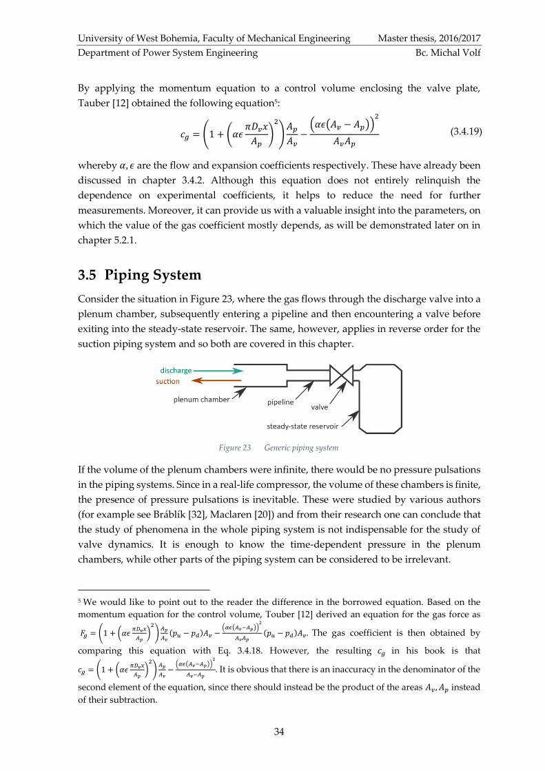
University of West Bohemia, Faculty of Mechanical Engineering Master thesis, 2016/2017
Department of Power System Engineering Bc. Michal Volf
34
By applying the momentum equation to a control volume enclosing the valve plate,
Tauber [12] obtained the following equation5:
𝑐𝑔 = (1 + (𝛼𝜖𝜋𝐷𝑣𝑥
𝐴𝑝)
2
)𝐴𝑝
𝐴𝑣−
(𝛼𝜖(𝐴𝑣 − 𝐴𝑝))2
𝐴𝑣𝐴𝑝 (3.4.19)
whereby 𝛼, 𝜖 are the flow and expansion coefficients respectively. These have already been
discussed in chapter 3.4.2. Although this equation does not entirely relinquish the
dependence on experimental coefficients, it helps to reduce the need for further
measurements. Moreover, it can provide us with a valuable insight into the parameters, on
which the value of the gas coefficient mostly depends, as will be demonstrated later on in
chapter 5.2.1.
3.5 Piping System
Consider the situation in Figure 23, where the gas flows through the discharge valve into a
plenum chamber, subsequently entering a pipeline and then encountering a valve before
exiting into the steady-state reservoir. The same, however, applies in reverse order for the
suction piping system and so both are covered in this chapter.
If the volume of the plenum chambers were infinite, there would be no pressure pulsations
in the piping systems. Since in a real-life compressor, the volume of these chambers is finite,
the presence of pressure pulsations is inevitable. These were studied by various authors
(for example see Bráblík [32], Maclaren [20]) and from their research one can conclude that
the study of phenomena in the whole piping system is not indispensable for the study of
valve dynamics. It is enough to know the time-dependent pressure in the plenum
chambers, while other parts of the piping system can be considered to be irrelevant.
5 We would like to point out to the reader the difference in the borrowed equation. Based on the
momentum equation for the control volume, Touber [12] derived an equation for the gas force as
𝐹𝑔 = (1 + (𝛼𝜖𝜋𝐷𝑣𝑥
𝐴𝑝)
2
)𝐴𝑝
𝐴𝑣
(𝑝𝑢 − 𝑝𝑑)𝐴𝑣 −(𝛼𝜖(𝐴𝑣−𝐴𝑝))
2
𝐴𝑣𝐴𝑝
(𝑝𝑢 − 𝑝𝑑)𝐴𝑣. The gas coefficient is then obtained by
comparing this equation with Eq. 3.4.18. However, the resulting 𝑐𝑔 in his book is that
𝑐𝑔 = (1 + (𝛼𝜖𝜋𝐷𝑣𝑥
𝐴𝑝)
2
)𝐴𝑝
𝐴𝑣−
(𝛼𝜖(𝐴𝑣−𝐴𝑝))2
𝐴𝑣−𝐴𝑝. It is obvious that there is an inaccuracy in the denominator of the
second element of the equation, since there should instead be the product of the areas 𝐴𝑣 , 𝐴𝑝 instead
of their subtraction.
Figure 23 Generic piping system

University of West Bohemia, Faculty of Mechanical Engineering Master thesis, 2016/2017
Department of Power System Engineering Bc. Michal Volf
35
Hence, it is justifiable to replace the entire piping system with a much simpler, but still
satisfactory, replacement - the single degree of freedom oscillator, in which the gas in the
plenum chamber acts as a spring, whereupon it is considered to be compressible, and the
fluid in the pipeline acts as a mass, after which it is assumed to be incompressible,
see Figure 24.
This method of accounting for the influence of pressure pulsations is extensively discussed,
including an experimental comparison, in a book by Touber [12] and thus only the main
idea of the model and the equations involved in it are summarized here.
Pipeline
The pipe is modelled as a straight one of length 𝐿𝑝𝑖𝑝𝑒 with a constant cross-sectional area
𝐴𝑝𝑖𝑝𝑒. It is assumed to be one-dimensional incompressible flow inside, the motion of which
(as a gas column) is governed by Newton’s second law:
𝑚𝑑𝑢
𝑑𝑡= ∑ 𝐹 (3.5.1)
where 𝑚 stands for the mass of the gas, 𝑢 means its velocity and ∑ 𝐹 denotes the sum of
forces acting on the gas column. Since 𝐴𝑝𝑖𝑝𝑒 is constant, one can divide with it Eq. 3.5.1 and
so the following can be obtained:
𝑚
𝐴𝑝𝑖𝑝𝑒2
𝑑(𝑢𝐴𝑝𝑖𝑝𝑒)
𝑑𝑡= ∑ 𝑝 = 𝑝1 − 𝑝2 − Δ𝑝𝑑𝑟𝑜𝑝 (3.5.2)
wherein 𝑚
𝐴𝑝𝑖𝑝𝑒2 = 𝑚𝑎 is referred to as acoustical mass, pressures 𝑝1, 𝑝2 are stagnation pressures
in the spaces connected by the pipeline, Δ𝑝𝑑𝑟𝑜𝑝 stands for the pressure drop in
the pipe (see Eq. 3.5.3).
Δ𝑝𝑑𝑟𝑜𝑝 = 𝜉1
2𝜌𝑢2 = (𝜆
𝐿𝑝𝑖𝑝𝑒
𝐷𝑝𝑖𝑝𝑒+ ∑ 𝐾)
1
2𝜌𝑢2 (3.5.3)
where the first element in the parenthesis stands for major losses due to friction, the other
one in the parenthesis for minor losses resulting from a local resistance.
By combining Eq. 3.5.2 with Eq. 3.5.3, one can obtain the flow equation in its general form:
𝑑Θ
𝑑𝑡=
𝐴𝑝𝑖𝑝𝑒
𝐿𝑝𝑖𝑝𝑒
(𝑝1 − 𝑝2) −𝜉
2𝜌𝐿𝑝𝑖𝑝𝑒𝐴𝑝𝑖𝑝𝑒Θ2 (3.5.4)
The drawback resulting from the simplification is that, since the value of 𝜌 is constant
throughout the length of the pipe, this generally leads to discontinuities at both ends of the
pipe. This can be solved with a further assumption that 𝜌 equals to an upstream value of
Figure 24 Helmholtz resonator concept

University of West Bohemia, Faculty of Mechanical Engineering Master thesis, 2016/2017
Department of Power System Engineering Bc. Michal Volf
36
𝜌1, a downstream value of 𝜌2 or to an average of 𝜌1 and 𝜌2. Based on experiments, the cited
author suggests utilizing the former approach.
Plenum Chambers
Fundamentally, the thermodynamic process inside the plenum chambers is entirely
analogous (even with the simplifications) to the one inside the compressor cylinder
discussed in chapter 3.3. Moreover, the volume of the plenum chambers is constant in time.
Regarding the suction plenum chamber and suction phase (Figure 25), the following equations
can be derived:
𝑑𝑝𝑠
𝑑𝑡=
𝜅
𝑉𝑠(
𝑝𝑠0
𝜌𝑠0Θ𝑠 −
𝑝𝑠
𝜌𝑠Θ𝑐𝑠) (3.5.5)
wherein 𝑉𝑠 is the volume of the suction plenum chamber, Θs =𝑑𝑚𝑖𝑛
𝑑𝑡 and Θ𝑐𝑠 =
𝑑𝑚𝑐
𝑑𝑡|
𝑠𝑢𝑐𝑡𝑖𝑜𝑛 .
The mass flow going in and out of the plenum chamber is linked to the mass of the gas
inside the plenum chamber, which is governed by the law of conservation of mass, i.e.:
𝑑𝜌𝑠
𝑑𝑡=
1
𝑉𝑠
(Θ𝑠 − Θ𝑐𝑠) (3.5.6)
It shall be pointed out, that Eqs. 3.5.5 and 3.5.6, which are explicitly intended for suction
phase, reduce for other phases since if the suction valve is closed, then Θ𝑐𝑠 equals zero.
Analogously to the preceding suction chamber, in case of the discharge plenum chamber and
discharge phase (Figure 26), the following equations can be written as:
𝑑𝑝𝑑
𝑑𝑡= −
𝜅
𝑉𝑑(
𝑝𝑑
𝜌𝑑Θ𝑑 −
𝑝𝑐
𝜌𝑐Θ𝑐𝑑) (3.5.7)
𝑑𝜌𝑑
𝑑𝑡= −
1
𝑉𝑑
(Θ𝑑 − Θ𝑐𝑑) (3.5.8)
where 𝑉𝑑 is the volume of the discharge plenum chamber, Θd =𝑑𝑚𝑜𝑢𝑡
𝑑𝑡 and
Θ𝑐𝑑 = −𝑑𝑚𝑐
𝑑𝑡|
𝑑𝑖𝑠𝑐ℎ𝑎𝑟𝑔𝑒 . Moreover, if the discharge valve is closed the Eqs. 3.5.7 and 3.5.8
reduce since Θ𝑐𝑑 equals zero.
Correction of the Model
It is necessary to say that this means of replacing the suction and discharge piping system
with a one-degree of freedom oscillator, will not agree in every detail with the real-life case.
However, one should bear in mind that this is not required either. It is quite enough if the
Figure 25 Suction plenum chamber Figure 26 Discharge plenum chamber

University of West Bohemia, Faculty of Mechanical Engineering Master thesis, 2016/2017
Department of Power System Engineering Bc. Michal Volf
37
deviation from the real case is low enough so as to permit the prediction of influencing the
valve plate behavior. To mitigate this deviation, the cited author proposes (on a theoretical
basis) a means of converting the dimensions of the real piping system to the ones used in
the equations above, i.e. 𝐿𝑝𝑖𝑝𝑒, 𝐴𝑝𝑖𝑝𝑒 and thus the interested reader is referred to the
source [12].
3.6 Periodical Quantities
In light of what was written in chapter 3.1.1 above anent not granting attention to the
periodical quantities (i.e. the quantities, the value of which is related to the entire
compressor cycle), we may perhaps be forgiven for calling attention here to some of them
since they will later on help us to follow the trends of the concepts and models discussed
previously. Specifically, a brief overview of three periodical quantities is presented here –
indicated work, indicated valve work and volumetric efficiency.
3.6.1 Indicated Work
The work, which is transmitted by the piston to the gas in the cylinder over the entire
compressor cycle, is given by the commonly-known equation:
𝑊𝑖 = ∮ 𝑝𝑐𝑑𝑉𝑐 = 𝐴𝑐 ∮ 𝑝𝑐𝑑𝑧 (3.6.1)
Considering the form, in which other equations were derived, it will be more convenient to
use the differential form of Eq. 3.6.1, i.e.:
𝑑𝑊𝑖
𝑑𝑡= 𝐴𝑐𝑝𝑐
𝑑𝑧
𝑑𝑡= 𝐴𝑐𝑝𝑐𝑤𝑧 (3.6.2)
3.6.2 Indicated Valve Work
The indicated valve work, i.e. the part of the indicated work connected with the pressure
drop across the valves, can be expressed analogously to the previous; however, it is
necessary to differentiate between the suction and discharge phases. Hence, the resulting
equations in differential form are respectively:
𝑑𝑊𝑖𝑣
𝑑𝑡|
𝑠𝑢𝑐𝑡𝑖𝑜𝑛= (𝑝𝑠 − 𝑝𝑐)𝐴𝑐|𝑤𝑧| (3.6.3)
𝑑𝑊𝑖𝑣
𝑑𝑡|
𝑑𝑖𝑠𝑐ℎ𝑎𝑟𝑔𝑒= (𝑝𝑐 − 𝑝𝑑)𝐴𝑐|𝑤𝑧| (3.6.4)
wherein the absolute value of the piston velocity 𝑤𝑧 is used so that the late valve closing is
not reflected in the indicated valve work. These equations will be integrated solely during
the suction (Eq. 3.6.3) or discharge (Eq. 3.6.4) phases of the compressor cycle.
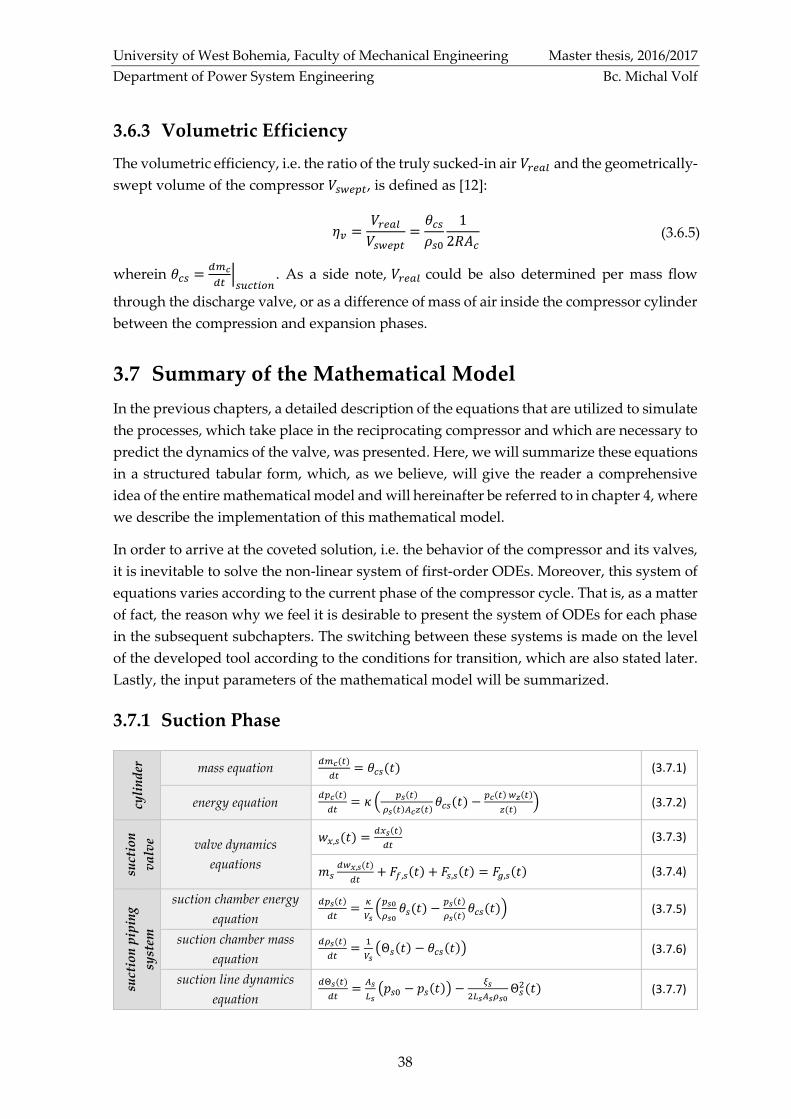
University of West Bohemia, Faculty of Mechanical Engineering Master thesis, 2016/2017
Department of Power System Engineering Bc. Michal Volf
38
3.6.3 Volumetric Efficiency
The volumetric efficiency, i.e. the ratio of the truly sucked-in air 𝑉𝑟𝑒𝑎𝑙 and the geometrically-
swept volume of the compressor 𝑉𝑠𝑤𝑒𝑝𝑡, is defined as [12]:
𝜂𝑣 =𝑉𝑟𝑒𝑎𝑙
𝑉𝑠𝑤𝑒𝑝𝑡=
𝜃𝑐𝑠
𝜌𝑠0
1
2𝑅𝐴𝑐 (3.6.5)
wherein 𝜃𝑐𝑠 =𝑑𝑚𝑐
𝑑𝑡|
𝑠𝑢𝑐𝑡𝑖𝑜𝑛. As a side note, 𝑉𝑟𝑒𝑎𝑙 could be also determined per mass flow
through the discharge valve, or as a difference of mass of air inside the compressor cylinder
between the compression and expansion phases.
3.7 Summary of the Mathematical Model
In the previous chapters, a detailed description of the equations that are utilized to simulate
the processes, which take place in the reciprocating compressor and which are necessary to
predict the dynamics of the valve, was presented. Here, we will summarize these equations
in a structured tabular form, which, as we believe, will give the reader a comprehensive
idea of the entire mathematical model and will hereinafter be referred to in chapter 4, where
we describe the implementation of this mathematical model.
In order to arrive at the coveted solution, i.e. the behavior of the compressor and its valves,
it is inevitable to solve the non-linear system of first-order ODEs. Moreover, this system of
equations varies according to the current phase of the compressor cycle. That is, as a matter
of fact, the reason why we feel it is desirable to present the system of ODEs for each phase
in the subsequent subchapters. The switching between these systems is made on the level
of the developed tool according to the conditions for transition, which are also stated later.
Lastly, the input parameters of the mathematical model will be summarized.
3.7.1 Suction Phase
cyli
nd
er
mass equation 𝑑𝑚𝑐(𝑡)
𝑑𝑡= 𝜃𝑐𝑠(𝑡) (3.7.1)
energy equation 𝑑𝑝𝑐(𝑡)
𝑑𝑡= 𝜅 (
𝑝𝑠(𝑡)
𝜌𝑠(𝑡)𝐴𝑐𝑧(𝑡)𝜃𝑐𝑠(𝑡) −
𝑝𝑐(𝑡) 𝑤𝑧(𝑡)
𝑧(𝑡)) (3.7.2)
suct
ion
va
lve valve dynamics
equations
𝑤𝑥,𝑠(𝑡) =𝑑𝑥𝑠(𝑡)
𝑑𝑡 (3.7.3)
𝑚𝑠𝑑𝑤𝑥,𝑠(𝑡)
𝑑𝑡+ 𝐹𝑓,𝑠(𝑡) + 𝐹𝑠,𝑠(𝑡) = 𝐹𝑔,𝑠(𝑡) (3.7.4)
suct
ion
pip
ing
syst
em
suction chamber energy
equation
𝑑𝑝𝑠(𝑡)
𝑑𝑡=
𝜅
𝑉𝑠(
𝑝𝑠0
𝜌𝑠0𝜃𝑠(𝑡) −
𝑝𝑠(𝑡)
𝜌𝑠(𝑡)𝜃𝑐𝑠(𝑡)) (3.7.5)
suction chamber mass
equation
𝑑𝜌𝑠(𝑡)
𝑑𝑡=
1
𝑉𝑠(Θ𝑠(𝑡) − 𝜃𝑐𝑠(𝑡)) (3.7.6)
suction line dynamics
equation
𝑑Θ𝑠(𝑡)
𝑑𝑡=
𝐴𝑠
𝐿𝑠(𝑝𝑠0 − 𝑝𝑠(𝑡)) −
𝜉𝑠
2𝐿𝑠𝐴𝑠𝜌𝑠0Θ𝑠
2(𝑡) (3.7.7)
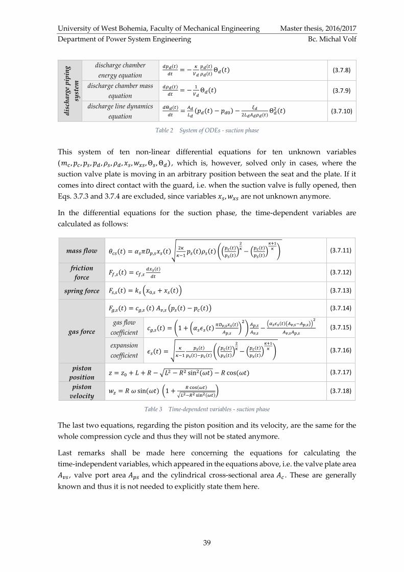
University of West Bohemia, Faculty of Mechanical Engineering Master thesis, 2016/2017
Department of Power System Engineering Bc. Michal Volf
39
dis
cha
rge
pip
ing
syst
em
discharge chamber
energy equation
𝑑𝑝𝑑(𝑡)
𝑑𝑡= −
𝜅
𝑉𝑑
𝑝𝑑(𝑡)
𝜌𝑑(𝑡)Θ𝑑(𝑡) (3.7.8)
discharge chamber mass
equation
𝑑𝜌𝑑(𝑡)
𝑑𝑡= −
1
𝑉𝑑Θ𝑑(𝑡) (3.7.9)
discharge line dynamics
equation
𝑑Θ𝑑(𝑡)
𝑑𝑡=
𝐴𝑑
𝐿𝑑(𝑝𝑑(𝑡) − 𝑝𝑑0) −
𝜉𝑑
2𝐿𝑑𝐴𝑑𝜌𝑑(𝑡)Θ𝑑
2 (𝑡) (3.7.10)
Table 2 System of ODEs - suction phase
This system of ten non-linear differential equations for ten unknown variables
(𝑚𝑐 , 𝑝𝑐 , 𝑝𝑠, 𝑝𝑑 , 𝜌𝑠, 𝜌𝑑 , 𝑥𝑠 , 𝑤𝑥𝑠, Θ𝑠, Θ𝑑) , which is, however, solved only in cases, where the
suction valve plate is moving in an arbitrary position between the seat and the plate. If it
comes into direct contact with the guard, i.e. when the suction valve is fully opened, then
Eqs. 3.7.3 and 3.7.4 are excluded, since variables 𝑥𝑠, 𝑤𝑥𝑠 are not unknown anymore.
In the differential equations for the suction phase, the time-dependent variables are
calculated as follows:
mass flow 𝜃𝑐𝑠(𝑡) = 𝛼𝑠𝜋𝐷𝑝,𝑠𝑥𝑠(𝑡)√2𝜅
𝜅−1𝑝𝑠(𝑡)𝜌𝑠(𝑡) ((
𝑝𝑐(𝑡)
𝑝𝑠(𝑡))
2
𝜅− (
𝑝𝑐(𝑡)
𝑝𝑠(𝑡))
𝜅+1
𝜅) (3.7.11)
friction
force 𝐹𝑓,𝑠(𝑡) = 𝑐𝑓,𝑠
𝑑𝑥𝑠(𝑡)
𝑑𝑡 (3.7.12)
spring force 𝐹𝑠,𝑠(𝑡) = 𝑘𝑠 (𝑥0,𝑠 + 𝑥𝑠(𝑡)) (3.7.13)
gas force
𝐹𝑔,𝑠(𝑡) = 𝑐𝑔,𝑠 (𝑡) 𝐴𝑣,𝑠 (𝑝𝑠(𝑡) − 𝑝𝑐(𝑡)) (3.7.14)
gas flow
coefficient 𝑐𝑔,𝑠(𝑡) = (1 + (𝛼𝑠𝜖𝑠(𝑡)
𝜋𝐷𝑣,𝑠𝑥𝑠(𝑡)
𝐴𝑝,𝑠)
2
)𝐴𝑝,𝑠
𝐴𝑣,𝑠−
(𝛼𝑠𝜖𝑠(𝑡)(𝐴𝑣,𝑠−𝐴𝑝,𝑠))2
𝐴𝑣,𝑠𝐴𝑝,𝑠 (3.7.15)
expansion
coefficient 𝜖𝑠(𝑡) = √
𝜅
𝜅−1
𝑝𝑠(𝑡)
𝑝𝑠(𝑡)−𝑝𝑐(𝑡)((
𝑝𝑐(𝑡)
𝑝𝑠(𝑡))
2
𝜅− (
𝑝𝑐(𝑡)
𝑝𝑠(𝑡))
𝜅+1
𝜅) (3.7.16)
piston
position 𝑧 = 𝑧0 + 𝐿 + 𝑅 − √𝐿2 − 𝑅2 sin2(𝜔𝑡) − 𝑅 cos(𝜔𝑡) (3.7.17)
piston
velocity 𝑤𝑧 = 𝑅 𝜔 sin(𝜔𝑡) (1 +
𝑅 cos(𝜔𝑡)
√𝐿2−𝑅2 sin2(𝜔𝑡)) (3.7.18)
Table 3 Time-dependent variables - suction phase
The last two equations, regarding the piston position and its velocity, are the same for the
whole compression cycle and thus they will not be stated anymore.
Last remarks shall be made here concerning the equations for calculating the
time-independent variables, which appeared in the equations above, i.e. the valve plate area
𝐴𝑣𝑠 , valve port area 𝐴𝑝𝑠 and the cylindrical cross-sectional area 𝐴𝑐 . These are generally
known and thus it is not needed to explicitly state them here.

University of West Bohemia, Faculty of Mechanical Engineering Master thesis, 2016/2017
Department of Power System Engineering Bc. Michal Volf
40
3.7.2 Discharge Phase cy
lin
der
mass equation 𝑑𝑚𝑐(𝑡)
𝑑𝑡= −𝜃𝑐𝑑(𝑡) (3.7.19)
energy equation 𝑑𝑝𝑐(𝑡)
𝑑𝑡= −𝜅 (
𝑝𝑐(𝑡)
𝜌𝑐(𝑡)𝐴𝑐𝑧(𝑡)𝜃𝑐𝑑 +
𝑝𝑐(𝑡) 𝑤𝑧(𝑡)
𝑧(𝑡)) (3.7.20)
dis
cha
rge
va
lve valve dynamics
equations
𝑤𝑥,𝑑(𝑡) =𝑑𝑥𝑑(𝑡)
𝑑𝑡 (3.7.21)
𝑚𝑑𝑑𝑤𝑥,𝑑(𝑡)
𝑑𝑡+ 𝐹𝑓,𝑑(𝑡) + 𝐹𝑠,𝑑(𝑡) = 𝐹𝑔,𝑑(𝑡) (3.7.22)
suct
ion
pip
ing
syst
em
suction chamber energy
equation
𝑑𝑝𝑠(𝑡)
𝑑𝑡=
𝜅
𝑉𝑠
𝑝𝑠0
𝜌𝑠0 𝜃𝑠(𝑡) (3.7.23)
suction chamber mass
equation
𝑑𝜌𝑠(𝑡)
𝑑𝑡=
1
𝑉𝑠Θ𝑠(𝑡) (3.7.24)
suction line dynamics
equation
𝑑Θ𝑠(𝑡)
𝑑𝑡=
𝐴𝑠
𝐿𝑠(𝑝𝑠0 − 𝑝𝑠(𝑡)) −
𝜉𝑠
2𝐿𝑠𝐴𝑠𝜌𝑠0Θ𝑠
2(𝑡) (3.7.25)
dis
cha
rge
pip
ing
syst
em
discharge chamber
energy equation
𝑑𝑝𝑑(𝑡)
𝑑𝑡= −
𝜅
𝑉𝑑 (
𝑝𝑑(𝑡)
𝜌𝑑(𝑡)Θ𝑑(𝑡) −
𝑝𝑐(𝑡)
𝜌𝑐(𝑡)Θ𝑐𝑑(𝑡)) (3.7.26)
discharge chamber mass
equation
𝑑𝜌𝑑(𝑡)
𝑑𝑡= −
1
𝑉𝑑(Θ𝑑(𝑡) − Θ𝑐𝑑(𝑡)) (3.7.27)
discharge line dynamics
equation
𝑑Θ𝑑(𝑡)
𝑑𝑡=
𝐴𝑑
𝐿𝑑(𝑝𝑑(𝑡) − 𝑝𝑑0) −
𝜉𝑑
2𝐿𝑑𝐴𝑑𝜌𝑑(𝑡)Θ𝑑
2 (𝑡) (3.7.28)
Table 4 System of ODEs - discharge phase
Similarly to the preceding phase, these ten ODEs form a non-linear system with ten
unknown variables, which are, however, in cases where the discharge phase takes place,
slightly different; namely 𝑚𝑐 , 𝑝𝑐 , 𝑝𝑠, 𝑝𝑑 , 𝜌𝑠, 𝜌𝑑 , 𝑥𝑑 , 𝑤𝑥𝑑, Θ𝑠, Θ𝑑.
The time-dependent variables in these differential equations are calculated as follows:
mass flow 𝜃𝑐𝑑(𝑡) = 𝛼𝑑𝜋𝐷𝑝,𝑑𝑥𝑑(𝑡)√2𝜅
𝜅−1𝑝𝑐(𝑡)𝜌𝑐(𝑡) ((
𝑝𝑑(𝑡)
𝑝𝑐(𝑡))
2
𝜅− (
𝑝𝑑(𝑡)
𝑝𝑐(𝑡))
𝜅+1
𝜅) (3.7.29)
friction
force 𝐹𝑓,𝑑(𝑡) = 𝑐𝑓,𝑑
𝑑𝑥𝑑(𝑡)
𝑑𝑡 (3.7.30)
spring force 𝐹𝑠,𝑑(𝑡) = 𝑘𝑑 (𝑥0,𝑑 + 𝑥𝑑(𝑡)) (3.7.31)
gas force
𝐹𝑔,𝑑(𝑡) = 𝑐𝑔,𝑑(𝑡) 𝐴𝑣,𝑑 (𝑝𝑐(𝑡) − 𝑝𝑑(𝑡)) (3.7.32)
gas flow
coefficient 𝑐𝑔,𝑑(𝑡) = (1 + (𝛼𝑑𝜖𝑑(𝑡)
𝜋𝐷𝑣,𝑑𝑥𝑑(𝑡)
𝐴𝑝,𝑑)
2
)𝐴𝑝,𝑑
𝐴𝑣,𝑑−
(𝛼𝑑𝜖𝑑(𝑡)(𝐴𝑣,𝑑−𝐴𝑝,𝑑))2
𝐴𝑣,𝑑𝐴𝑝,𝑑 (3.7.33)
expansion
coefficient 𝜖𝑑(𝑡) = √
𝜅
𝜅−1
𝑝𝑐(𝑡)
𝑝𝑐(𝑡)−𝑝𝑑(𝑡)((
𝑝𝑑(𝑡)
𝑝𝑐(𝑡))
2
𝜅− (
𝑝𝑑(𝑡)
𝑝𝑐(𝑡))
𝜅+1
𝜅) (3.7.34)
Table 5 Time-dependent variables - discharge phase
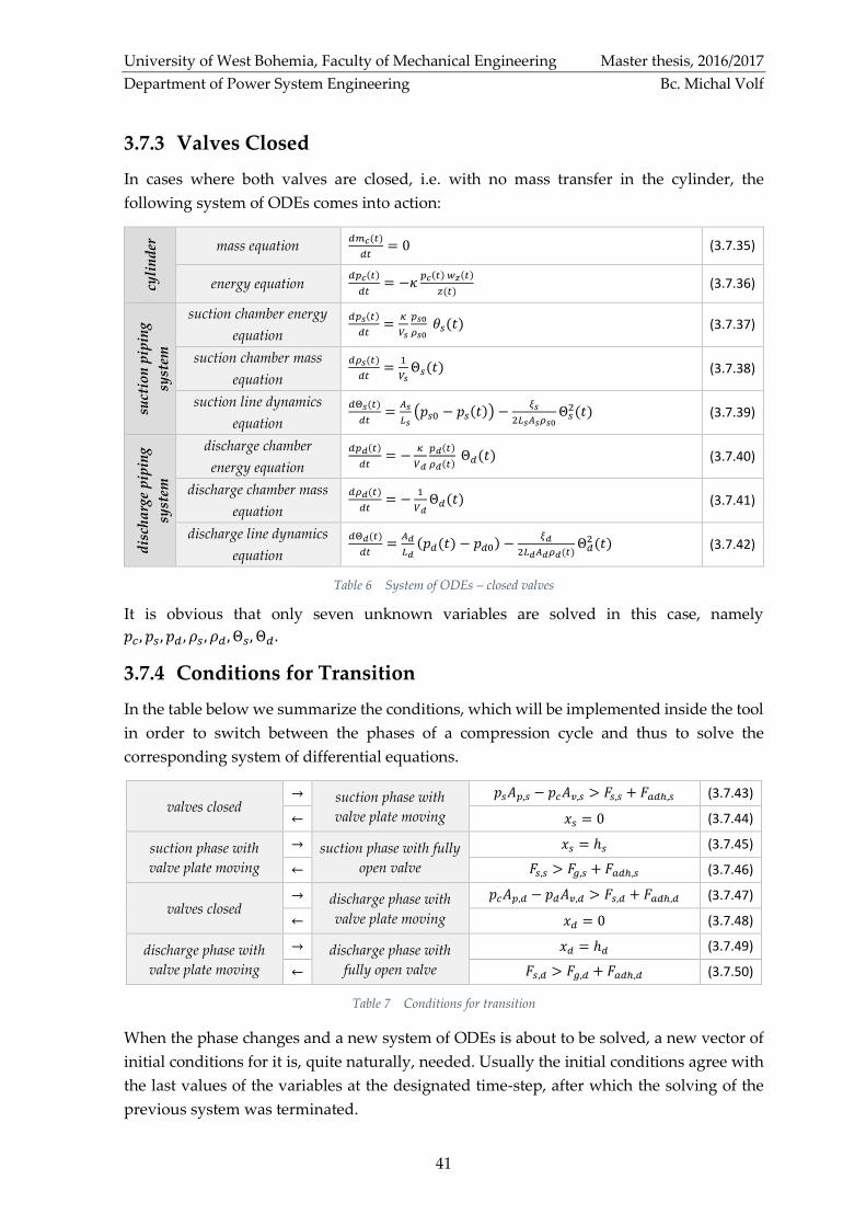
University of West Bohemia, Faculty of Mechanical Engineering Master thesis, 2016/2017
Department of Power System Engineering Bc. Michal Volf
41
3.7.3 Valves Closed
In cases where both valves are closed, i.e. with no mass transfer in the cylinder, the
following system of ODEs comes into action:
cyli
nd
er
mass equation 𝑑𝑚𝑐(𝑡)
𝑑𝑡= 0 (3.7.35)
energy equation 𝑑𝑝𝑐(𝑡)
𝑑𝑡= −𝜅
𝑝𝑐(𝑡) 𝑤𝑧(𝑡)
𝑧(𝑡) (3.7.36)
suct
ion
pip
ing
syst
em
suction chamber energy
equation
𝑑𝑝𝑠(𝑡)
𝑑𝑡=
𝜅
𝑉𝑠
𝑝𝑠0
𝜌𝑠0 𝜃𝑠(𝑡) (3.7.37)
suction chamber mass
equation
𝑑𝜌𝑠(𝑡)
𝑑𝑡=
1
𝑉𝑠Θ𝑠(𝑡) (3.7.38)
suction line dynamics
equation
𝑑Θ𝑠(𝑡)
𝑑𝑡=
𝐴𝑠
𝐿𝑠(𝑝𝑠0 − 𝑝𝑠(𝑡)) −
𝜉𝑠
2𝐿𝑠𝐴𝑠𝜌𝑠0Θ𝑠
2(𝑡) (3.7.39)
dis
cha
rge
pip
ing
syst
em
discharge chamber
energy equation
𝑑𝑝𝑑(𝑡)
𝑑𝑡= −
𝜅
𝑉𝑑
𝑝𝑑(𝑡)
𝜌𝑑(𝑡) Θ𝑑(𝑡) (3.7.40)
discharge chamber mass
equation
𝑑𝜌𝑑(𝑡)
𝑑𝑡= −
1
𝑉𝑑Θ𝑑(𝑡) (3.7.41)
discharge line dynamics
equation
𝑑Θ𝑑(𝑡)
𝑑𝑡=
𝐴𝑑
𝐿𝑑(𝑝𝑑(𝑡) − 𝑝𝑑0) −
𝜉𝑑
2𝐿𝑑𝐴𝑑𝜌𝑑(𝑡)Θ𝑑
2 (𝑡) (3.7.42)
Table 6 System of ODEs – closed valves
It is obvious that only seven unknown variables are solved in this case, namely
𝑝𝑐 , 𝑝𝑠, 𝑝𝑑 , 𝜌𝑠, 𝜌𝑑 , Θ𝑠, Θ𝑑 .
3.7.4 Conditions for Transition
In the table below we summarize the conditions, which will be implemented inside the tool
in order to switch between the phases of a compression cycle and thus to solve the
corresponding system of differential equations.
valves closed → suction phase with
valve plate moving
𝑝𝑠𝐴𝑝,𝑠 − 𝑝𝑐𝐴𝑣,𝑠 > 𝐹𝑠,𝑠 + 𝐹𝑎𝑑ℎ,𝑠 (3.7.43)
← 𝑥𝑠 = 0 (3.7.44)
suction phase with
valve plate moving
→ suction phase with fully
open valve
𝑥𝑠 = ℎ𝑠 (3.7.45)
← 𝐹𝑠,𝑠 > 𝐹𝑔,𝑠 + 𝐹𝑎𝑑ℎ,𝑠 (3.7.46)
valves closed → discharge phase with
valve plate moving
𝑝𝑐𝐴𝑝,𝑑 − 𝑝𝑑𝐴𝑣,𝑑 > 𝐹𝑠,𝑑 + 𝐹𝑎𝑑ℎ,𝑑 (3.7.47)
← 𝑥𝑑 = 0 (3.7.48)
discharge phase with
valve plate moving
→ discharge phase with
fully open valve
𝑥𝑑 = ℎ𝑑 (3.7.49)
← 𝐹𝑠,𝑑 > 𝐹𝑔,𝑑 + 𝐹𝑎𝑑ℎ,𝑑 (3.7.50)
Table 7 Conditions for transition
When the phase changes and a new system of ODEs is about to be solved, a new vector of
initial conditions for it is, quite naturally, needed. Usually the initial conditions agree with
the last values of the variables at the designated time-step, after which the solving of the
previous system was terminated.

University of West Bohemia, Faculty of Mechanical Engineering Master thesis, 2016/2017
Department of Power System Engineering Bc. Michal Volf
42
An exception lies in the case where a phase transition will be made based on Eqs. 3.7.44,
3.7.45, 3.7.48 or 3.7.49, where one must deal with a rebound before the transition can
proceed. This means that when a valve plate touches an obstacle (seat or guard), the phase
will not change immediately and instead the same system of differential equations will be
solved anew, however, with the initial conditions, in which the initial velocity of the plate
will be calculated as −𝑐𝑟𝑤𝑙𝑎𝑠𝑡, wherein 𝑐𝑟 stands for the coefficient of restitution and 𝑤𝑙𝑎𝑠𝑡
denotes the velocity in the moment of impact. This is repeated until the initial velocity is
very low, then the phase transition will proceed. For the actual implementation, see
chapter 4.3.1.
3.7.5 Input Parameters
Finally, lets summarize the variables, which are considered to be input parameters in the
mathematical model, i.e. the value of all these forty parameters has to be given. Bear in
mind that all of them are required to be in basic SI units in the developed simulation tool.
Ideal gas Discharge valve
heat capacity ratio 𝜅 spring preload deflection 𝑥0,𝑑
ideal gas constant 𝑟 maximum valve plate lift ℎ𝑑
Crank mechanism spring stiffness 𝑘𝑑
connecting rod length 𝐿 mass (plate with equivalent of spring) 𝑚𝑑
cylinder diameter 𝐷𝑐 valve plate diameter 𝐷𝑣,𝑑
clearance length 𝑧0 valve port diameter 𝐷𝑝,𝑑
angular velocity of the crankshaft 𝜔 coefficient of restitution 𝑐𝑟,𝑑
radius of the crankshaft 𝑅 friction coefficient 𝑐𝑓,𝑑
Suction valve flow coefficient 𝛼𝑑
spring preload deflection 𝑥0,𝑠 Suction piping system
maximum valve plate lift ℎ𝑠 static pressure in steady-state reservoir 𝑝𝑠0
spring stiffness 𝑘𝑠 static temperature in the reservoir 𝑇𝑠0
mass (plate with equivalent of spring) 𝑚𝑠 volume of the suction chamber 𝑉𝑠
valve plate diameter 𝐷𝑣,𝑠 effective length of the suction pipe 𝐿𝑠
valve port diameter 𝐷𝑝,𝑠 effective cross-sectional area of the pipe 𝐴𝑠
coefficient of restitution 𝑐𝑟,𝑠 loss coefficient in the suction pipe 𝜉𝑠
friction coefficient 𝑐𝑓,𝑠 Discharge piping system
flow coefficient 𝛼𝑠 static pressure in steady-state reservoir 𝑝𝑑0
Adhesion static temperature in the reservoir 𝑇𝑑0
surface tension 𝛾𝐿𝐺 volume of the discharge chamber 𝑉𝑑
meniscus contact angle 𝛽 effective length of the discharge pipe 𝐿𝑑
oil film thickness ℎ𝑓𝑖𝑙𝑚 effective cross-sectional area of the pipe 𝐴𝑑
loss coefficient in the discharge pipe 𝜉𝑑
Table 8 Input parameters

University of West Bohemia, Faculty of Mechanical Engineering Master thesis, 2016/2017
Department of Power System Engineering Bc. Michal Volf
43
4 Developing the Simulation Tool
This chapter is devoted to the process of building the tool, in which the valve behavior is
predicted based on the given parameters of the compressor, the undertaking of which is the
third task of this thesis. Moreover, one can consider this section to be an elaboration of the
mathematical model, since in this chapter we bring the model to life.
Firstly, we discuss the structure of the program as well as the reasons why object-oriented
programming (OOP) is used; we then look at the way how the equations are handled and
the system into which it is integrated. Finally, the methods one can utilize to run the
simulator are presented.
One should bear in mind however, that the whole simulation tool is composed of more than
three thousand lines of code in total and thus it is impractical to describe the meaning of
every line in this text. However, this is not required anyway, because the code itself is
thoroughly and conscientiously annotated, so that one can easily figure out its functions.
Hence, only the main principles and ideas are discussed in the following subchapters, so
that the reader can grasp the concept of the tool and can not only use it properly but is also
able to further modify it, if the need arises.
Last but not least, the tool is built in the commercially available software MATLAB in
version 2016b, for which we own the student license. Be aware that the faultless functioning
of the tool in older versions of MATLAB cannot be guaranteed.
4.1 General Remarks
4.1.1 Simulation Tool Requirements
In the section regarding the Purpose of Research, it was stated that the mathematical model
should be implemented, while keeping its properties, i.e. its versatility and customizability.
The essential question is however, what do we mean by this? Regarding the latter, consider
the mathematical model as it was first proposed, i.e. that it includes various phenomena
(e.g. rebound, pressure pulsations in the piping etc.) while omitting others (e.g. heat
transfer through the cylinder etc.). If all of the equations describing these processes were to
be merged together - providing us with a system of ODEs to solve without other additional
ancillary equations - the model could very easily be implemented. But such an attitude
would result in a complete waste of customizability, since additional changes in the
equations would be, simply put, impractical. One could ask however, what about its
versatility? Recall the types of compressor models (chapter 3.1.2), in which the valve
dynamics can be studied. The model proposed in this thesis is a complete one, i.e. besides
other things it includes the influence of the piping system on valve dynamics. On the other
hand, the fly in the ointment here lies in the fact that in order to evaluate the influence rate,

University of West Bohemia, Faculty of Mechanical Engineering Master thesis, 2016/2017
Department of Power System Engineering Bc. Michal Volf
44
it is also indispensable to simulate the valve dynamics without the pressure pulsations. It
goes without saying that this holds true for other phenomena as well.
Among the phenomena, which influence valve behavior and are implemented in such a
way, that they can be excluded from the simulation, are the following:
• rebound
• friction
• adhesion
• pressure pulsations in piping systems
4.1.2 Object-Oriented Programming
To fulfill the requirements, it is basically essential to keep the equations separated and to
figure out a way how to combine them with ease in order to arrive at a system of equations
that can be eventually solved. Basically, two approaches seem to make sense; either
utilizing symbolic variables and expressions, or the use of function handles.
In the former method, the equations and variables would be defined as symbolic ones, then
they could automatically be merged together and thus a system of symbolic equations
would arise. However, since the system of ODEs, which is striven to be solved, is
non-linear, the solution generally cannot be found explicitly and one must rely on
numerical methods. Hence, the symbolic system must be converted to a non-symbolic one,
which can be solved numerically later on. This is actually the pitfall of this approach, since
according to our tests, the elapsed time needed to arrive at a solution is unsuitable, i.e. more
than 25x higher in comparison with the latter approach.6
The latter approach, which is applied in this thesis, works on the presumption that the
equations could be merged through function handles and thus evading the need for
symbolic expressions. Simply put, instead of using substitution from one equation to
another, function handles are used as input arguments for other functions; a detailed
example is given in section 4.2.2.2. The merit of this method lies in the fact that one can
avoid the conversion between symbolic and non-symbolic notation and thus rapidly reduce
the computational time, but the drawback is that the code could very easily become
unreadable and tangled, if not implemented properly.
The decision to utilize the programming paradigm based on the concept of objects seems
now rather straightforward since it provides us with an elegant way to maintain the desired
characteristics of the tool while keeping the code well-structured and thus easily readable.
As a matter of fact, the OOP could help us achieve much more (such as data protection,
general pattern creation and so on.), if we pursued things like encapsulation, inheritance,
6 Bear in mind that the elapsed time for solving the equations (for one compressor cycle) in the last
version of the tool is about three minutes (measured on a PC with 8 GB of RAM, Intel Core
i7-3720QM) and thus with the symbolic approach, the elapsed time could easily exceed one hour.

University of West Bohemia, Faculty of Mechanical Engineering Master thesis, 2016/2017
Department of Power System Engineering Bc. Michal Volf
45
or polymorphism. However, it would be, on the one hand, far beyond the scope of this
thesis, and on the other hand, there would be no benefit for the purpose of study of valve
behavior.
4.1.3 Structure of the Tool
The file structure of the tool comprises four files, namely
• ReciprocatingCompressor_app.mlapp
• runTool.m
• ReciprocatingCompressor_class.m
• defaultParameters.m
Either one of the former two files can be used to run the tool; these are discussed later in
corresponding chapter 4.4. In the meantime, we will go through the penultimate file, i.e.
ReciprocatingCompressor_class.m, which contains all the crucial parts of the simulation tool,
i.e. from the assignment of equations, going through their solution and then on to the post-
processing. The lastly-named file represents an auxiliary function solely for defining
numerical values of input parameters and thus no special chapter is needed there.
4.2 Class Structure
The entire compressor model is implemented into a class (ReciprocatingCompressor_class.m),
which is derived from the generic handle class. The compressor class encapsulates the
properties and methods, i.e. the operations performed on the properties. The general
structure of this class is outlined in Figure 27.
4.2.1 Class Properties
Regarding the class properties, they are divided, mainly for the purpose of clarity, into two
categories and those in turn into subcategories. The first category, called the Mathematical
model stores data regarding the mathematical model. For example, in the first subcategory
called Constants, there are defined variables which are used later on to store the values of
the input data, i.e. the quantities already defined in Table 8. The constant quantities, which
are calculated from these input parameters, i.e. they do not change with time, are defined
in the second subcategory Constant Calculated Parameters. Then, there is a subcategory
labeled Type of Compressor, in which the variables, through which one can turn the effects
influencing valve dynamics on or off, are defined. These groups of properties discussed up
to now, are non-dependent properties, i.e. they store data. However, the last subcategory
marked as Time-dependent parameters & Equations unites dependent properties, i.e. their
value depends on some other value, such as time or the value of a non-dependent property.

University of West Bohemia, Faculty of Mechanical Engineering Master thesis, 2016/2017
Department of Power System Engineering Bc. Michal Volf
46
classdef ReciprocatingCompressor_class < handle
%% MATHEMATICAL MODEL
properties (Access = public) % Constants (Input data)
properties (Access = public) % Constant Calculated Parameters
properties (Access = public) % Type of Compressor
properties (Dependent = true) % Time-dependent parameters & Equations
%% TOOL PARAMETERS
properties (Access = public) % Constant Tool Parameters
properties (Dependent = true) % Time-dependent Tool Parameters
%% METHODS
methods
%% CLASS CONSTRUCTOR
function obj = ReciprocatingCompressor_developer(varargin)
%% GET-ACCESS METHODS FOR DEPENDENT PROPERTIES
%% Time-dependent Properties
%% Differential Equations
%% Conditions For Transition
%% SOLVING CYCLE & VALVE DYNAMICS
%% POST-PROCESSING
end
end
Figure 27 Structure of the compressor class
The second category, i.e. Tool Parameters is used to store data necessary for the flawless
function of the tool. It consists of two subcategories, where the first one unites the
non-dependent properties, e.g. the current phase of the compressor cycle etc., whereas the
second one stores the dependent properties, e.g. the number of completed compressor
cycles etc.
Bear in mind that our class properties merely define the name of variables, not their value.
Values are assigned later on either in a class constructor (for non-dependent properties) or
by get-access methods (for dependent properties).
4.2.2 Class Methods
The methods in the class are divided into four categories according to their purpose. Firstly,
there is a class constructer method needed to create instances of the class. Then, there is a
group of get-access methods, which are necessary to retrieve the value of the dependent
properties. The insight into these two types of methods is given later in this subchapter.
The third group unites the functions, which are requisite for handling either the transition
between the phases of the compression cycle (and thus the system of ODEs), or from the
perspective of the integration of the ODEs as such. Since the essence of the entire simulation

University of West Bohemia, Faculty of Mechanical Engineering Master thesis, 2016/2017
Department of Power System Engineering Bc. Michal Volf
47
tool lies in this part of the code, the detailed description of the process going on there is
given in a separate chapter 4.3.
Finally, there is a group in which are joined together methods for the post-processing of the
results, e.g. plotting the 𝑝 − 𝑉 diagram of the cycle, plotting the lift of valves as a function
of time, etc. Since these methods are very comprehensible, they are not described
further in-depth in the text of this thesis.
4.2.2.1 Class Constructor
In simple terms, a class provides a definition for objects of its type, i.e. it specifies certain
characteristics that all instances of that class share. To create an instance of a class with
initialized values of all the non-dependent properties, a special function, generally known
as the class constructor, is implicitly required. The name of this method must correspond to
the name of the class; hence, in our case its name is ReciprocatingCompressor_class.
The constructor accepts one input argument (Figure 28), thereby a structure array of values
of given input data. This structure array is created simultaneously with a function, which
can be found inside the file called defaultParameters.m. This way helps us to evade the
necessity to fill all the forty parameters into a class constructor syntax, which would be, at
least in our opinion, inconvenient.
newCompressor = ReciprocatingCompressor_class(parameters);
Figure 28 Class constructor (function syntax)
Barring the direct assignment of property values from the structure array, all the equations
for the calculation of values of the non-dependent quantities, such as valve port area, valve
plate area, etc., which are to be calculated only once during the initialization of the class
instance, are all found further inside this method.
4.2.2.2 Get-access Methods
Since dependent properties do not store data, for each one of them a get-access method needs
to be defined. Its function is to determine a value for the property when the property is
queried. However, by this value we do not strictly mean a numerical value, but rather the
equation according to which the numerical value of that property will be calculated later
on, during the moment when the system of ODEs is being solved. For this purpose, the
get-access methods in our class returns a function handle in most cases.
Get-access Methods for Equations
For a deeper understanding of linking the equations between each other, let us look at, for
example, a value for the dependent 𝑉𝑐 property (i.e. the cylinder volume), which depends
on the value of another dependent property 𝑧 (i.e. the piston displacement). The get-access
methods for both dependent properties are to be found below respectively.

University of West Bohemia, Faculty of Mechanical Engineering Master thesis, 2016/2017
Department of Power System Engineering Bc. Michal Volf
48
function value = get.V_c(obj) % Cylinder volume
value = @(vars) obj.A_c * obj.z(vars);
end
Figure 29 Get-access method for cylinder volume
function value = get.z(obj) % Piston dispacement
value = @(vars) obj.z_0 + obj.L + obj.R - ...
sqrt(obj.L^2-obj.R^2*(sin(obj.omega*vars.t)).^2) - ...
obj.R*cos(obj.omega*vars.t);
end
Figure 30 Get-access method for piston displacement
When the 𝑉𝑐 property is queried, the get.V_c method queries the 𝑧 property before
retrieving the 𝑉𝑐 property, i.e. result would eventually be following:
value = @(vars) obj.A_c * (obj.z_0 + obj.L + obj.R - ...
sqrt(obj.L^2-obj.R^2*(sin(obj.omega*vars.t)).^2) - ...
obj.R*cos(obj.omega*vars.t));
Figure 31 Resulting equation for cylinder volume
This example nicely shows the reader, how by calling the class properties representing the
equations between themselves, one can in a polished way link the equations together
without losing any of their potential customizability. For instance, if one wanted to simulate
the valve behavior in a compressor, in which the crank mechanism does not drive the piston
movement, he would basically only modify the equation concerning the 𝑧 property.
Furthermore, the get-access methods effortlessly allow us to handle the turning effects
influencing the valve behavior on or off. The illustration of this can be demonstrated on a
property, which stands for the friction force, see Figure 32.
function value = get.F_fs(obj) % Friction force – suction valve
if obj.dynamics_friction
value = @(vars) obj.c_fs*vars.v_xs;
else
value = @(vars) 0;
end
end
Figure 32 Get-access method for friction force (suction valve)
In this example the value, which the get-access method returns, depends on the logical value
of the property called dynamics_friction. If this value is false, then the get-access method
returns a zero value of the friction force, and thus this kind of force is not taken into account
at all.
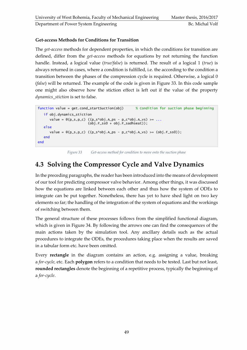
University of West Bohemia, Faculty of Mechanical Engineering Master thesis, 2016/2017
Department of Power System Engineering Bc. Michal Volf
49
Get-access Methods for Conditions for Transition
The get-access methods for dependent properties, in which the conditions for transition are
defined, differ from the get-access methods for equations by not returning the function
handle. Instead, a logical value (true/false) is returned. The result of a logical 1 (true) is
always returned in cases, where a condition is fulfilled, i.e. the according to the condition a
transition between the phases of the compression cycle is required. Otherwise, a logical 0
(false) will be returned. The example of the code is given in Figure 33. In this code sample
one might also observe how the stiction effect is left out if the value of the property
dynamics_stiction is set to false.
function value = get.cond_startSuction(obj) % Condition for suction phase beginning
if obj.dynamics_stiction
value = @(p_s,p_c) ((p_s*obj.A_ps - p_c*obj.A_vs) >= ... (obj.F_ss0 + obj.F_sadhseat)); else
value = @(p_s,p_c) ((p_s*obj.A_ps - p_c*obj.A_vs) >= (obj.F_ss0));
end
end
Figure 33 Get-access method for condition to move onto the suction phase
4.3 Solving the Compressor Cycle and Valve Dynamics
In the preceding paragraphs, the reader has been introduced into the means of development
of our tool for predicting compressor valve behavior. Among other things, it was discussed
how the equations are linked between each other and thus how the system of ODEs to
integrate can be put together. Nonetheless, there has yet to have shed light on two key
elements so far; the handling of the integration of the system of equations and the workings
of switching between them.
The general structure of these processes follows from the simplified functional diagram,
which is given in Figure 34. By following the arrows one can find the consequences of the
main actions taken by the simulation tool. Any ancillary details such as the actual
procedures to integrate the ODEs, the procedures taking place when the results are saved
in a tabular form etc. have been omitted.
Every rectangle in the diagram contains an action, e.g. assigning a value, breaking
a for-cycle, etc. Each polygon refers to a condition that needs to be tested. Last but not least,
rounded rectangles denote the beginning of a repetitive process, typically the beginning of
a for-cycle.

University of West Bohemia, Faculty of Mechanical Engineering Master thesis, 2016/2017
Department of Power System Engineering Bc. Michal Volf
50
Figure 34 Functional diagram of solving cycle & valve dynamics

University of West Bohemia, Faculty of Mechanical Engineering Master thesis, 2016/2017
Department of Power System Engineering Bc. Michal Volf
51
4.3.1 Switching Between Compressor Phases
From the mathematical model one can see that in order to obtain the valve behavior of the
entire compressor cycle, it is necessary to distinguish between the processes, from which
the cycle is composed of, i.e. suction, discharge, expansion and compression. Moreover, in
cases where either a suction or discharge phase takes place, one must also distinguish
whether the valve plate is in direct contact with the limiter or not. Furthermore, the
transition to the former cannot be done immediately, because initially a rebound must be
considered.
A certain simplification can be made regarding the expansion and compression, since the
mathematical description for these is the same. Hence, they can be generalized into a single
phase, which is henceforth labeled as valves closed. Furthermore, if we embrace a
prerequisite that the compressor cycle starts and ends at a point, when both valves are being
closed, then the suction/discharge phase with a fully open valve can be included as a
limiting case in the suction/discharge phase with the valve plate in motion. Hence, the
entire compressor cycle can be composed of three main phases; suction, discharge and valves
closed - as can be seen from the functional diagram. In the simulation tool, a property called
phase is defined, in which the ongoing phase of the compressor cycle is stored as a numerical
value. The relation between the compressor phase and to its corresponding numerical value
is listed in the following table.
suction phase with valve plate in motion 1
suction phase with fully open valve 1.5
discharge phase with valve plate in motion 2
discharge phase with fully open valve 2.5
valves closed 3
Table 9 Numerical representation of compressor phase
Naturally, several logic operations need to be carried out in order to determine the phase
transitions and so as to compose the corresponding system of ODEs that can be eventually
integrated. In the functional diagram, the conditions for transition are depicted in yellow
polygons within a for-cycle. Table 10 links their string representation (i.e. class property
name) to the actual equation from chapter 3.7.4. It is felt that it might be beneficial to not
include solely the reference number, but also the equation as such in that table, since it will
be needed shortly.

University of West Bohemia, Faculty of Mechanical Engineering Master thesis, 2016/2017
Department of Power System Engineering Bc. Michal Volf
52
Name of Condition Phase Transition Equation su
ctio
n suctionTerminate 1 → 3 (3.7.44) 𝑥𝑠 = 0
suctionFullyOpen 1 → 1.5 (3.7.45) 𝑥𝑠 = ℎ𝑠
suctionReleased 1.5 → 1 (3.7.46) 𝐹𝑠,𝑠 > 𝐹𝑔,𝑠 + 𝐹𝑎𝑑ℎ,𝑠
dis
cha
rge dischargeTerminate 2 → 3 (3.7.48) 𝑥𝑑 = 0
dischargeFullyOpen 2 → 2.5 (3.7.49) 𝑥𝑑 = ℎ𝑑
dischargeeReleased 2.5 → 2 (3.7.50) 𝐹𝑠,𝑑 > 𝐹𝑔,𝑑 + 𝐹𝑎𝑑ℎ,𝑑
va
lves
clo
sed
startSuction 3 → 1 (3.7.43) 𝑝𝑠𝐴𝑝,𝑠 − 𝑝𝑐𝐴𝑣,𝑠 > 𝐹𝑠,𝑠 + 𝐹𝑎𝑑ℎ,𝑠
startDischarge 3 → 2 (3.7.47) 𝑝𝑐𝐴𝑝,𝑑 − 𝑝𝑑𝐴𝑣,𝑑 > 𝐹𝑠,𝑑 + 𝐹𝑎𝑑ℎ,𝑑
Table 10 Condition for transitions - property names & equations
As mentioned before, in order to solve a non-linear system of differential equations, one
must typically rely on a numerical scheme to accurately approximate the solution.
Regardless of the numerical method, a solution will be obtained as a set of discrete points
instead of being continuous. This brings about a severe difficulty in the implementation of
the conditions for the transition, specifically the ones with the equal sign.
Consider the suction valve plate to be moving towards the seat, leaving aside a rebound for
a while. According to the conditions for the transition, in order to proceed from the suction
phase to the phase with closed valves, the valve plate lift must equal zero. However, the
resulting lift is in a form of discrete points (Figure 35) and thus, it would be irrational to
expect that the solution will be received at such a time point, when the valve plate lift equals
exactly zero. An analogous situation comes when the valve plate moves towards the limiter.
It follows that the conditions for the transition with the equal sign need to be modified, but
with regard to their meaning as well as to their physical admissibility. The altered
conditions for the transition are to be found in Table 11 and the explanation of the
implementation comes promptly afterwards.
Figure 35 Continuous & numerical solution

University of West Bohemia, Faculty of Mechanical Engineering Master thesis, 2016/2017
Department of Power System Engineering Bc. Michal Volf
53
Name of Condition Phase Transition Modified Equation
suction suctionTerminate 1 → 3 𝑥𝑠 ≤ 0
suctionFullyOpen 1 → 1.5 𝑥𝑠 ≥ ℎ𝑠
discharge dischargeTerminate 2 → 3 𝑥𝑑 ≤ 0
dischargeFullyOpen 2 → 2.5 𝑥𝑑 ≥ ℎ𝑑
Table 11 Modified conditions for transition
It goes without saying that such a modification allows us to implement with ease the
conditions for the transition; however, should no further action be carried out, the physical
admissibility will be lost, since the conditions will be, by a large majority, fulfilled thanks
to the inequality sign. It would mean, for example, that a condition is fulfilled when the
valve plate lift is negative, which is not possible from the physical point of view. To avoid
such dubious situations, an ingenious trick is used that one can figure out from the
functional diagram (Figure 34).
Basically, in every time-step it is tested whether the solution fulfills a condition for
transition related to the current compressor phase; if it does not then this solution is saved
into the results. However, should it fulfill a condition for transition, then the phase
transition proceeds but without saving the solution, since it is in all likelihood an
unphysical solution. The last-saved solution will be used for the composition of initial
conditions for the successive compressor phase; however, quantities such as valve plate lift
or its velocity will be adjusted so that they correspond to the exact value it was aimed at.
Apropos of this manual adjustment, there is virtually no influence over the results since
this is rather a cosmetic alteration of the results. For example, it was observed that in the
default compressor setup the difference between the last physical numerical solution of the
valve plate lift and its aimed value is less than one-ten-thousandth of the lift.
Rebound
In the subsequent paragraphs, we will shed light on the way how the rebound effect is
handled by the conditions for the transition. It is needless to say that in cases, where no
rebound applies, the phase transitions based on conditions suctionFullyOpen,
suctionTerminate, dischargeFullyOpen or dischargeTerminate will proceed instantly. However,
should rebound be considered, these aforesaid phase transitions need to be postponed until
the effect of rebound is over.
The rebound is to be taken into account through initial conditions indispensable for the
time-dependent system of ODEs, specifically the initial velocity, which is calculated per
Eq. 3.4.14 stated in chapter 3.4.3.3. This equation can be worded as follows: the initial valve
plate velocity for the succeeding phase is equal to its velocity prior to the impact multiplied
by the coefficient of restitution.

University of West Bohemia, Faculty of Mechanical Engineering Master thesis, 2016/2017
Department of Power System Engineering Bc. Michal Volf
54
Technically speaking, the valve plate will bounce unless the impact velocity equals zero. It
stands to reason that in real-life the bouncing effect is influenced and attenuated by other
factors such as oil film etc. and thus, should the rebound velocity be sufficiently small, one
can consider the bouncing effect to be overcome. In the same manner, the handling of the
rebound effect is implemented in the simulation tool. Hence, the meaning of the conditions
depicted in the functional diagram (Figure 34) in the light green polygons within a for-cycle
are stated in the following table:
Name of Condition Condition Allows phase transition
suctionRebound |𝑑𝑥𝑠
𝑑𝑡|
𝑡+| < 𝜖𝑠
1 → 1.5
1 → 3
dischargeRebound |𝑑𝑥𝑑
𝑑𝑡|
𝑡+| < 𝜖𝑑
2 → 2.5
2 → 3
Table 12 Conditions for rebound
Naturally, the magnitude of the tolerances 𝜖𝑠 and 𝜖𝑑 is the backbone of the decision
whether the phase transition can be carried out or not. The potential failure of the transition
towards a phase with a fully open valve does not bring about any issues, whereas the failure
of the transition towards the valves closed phase does. If this phase transition fails to carry
out, the simulator tool cannot terminate the solving of compressor cycle due to the
presumption that the compressor cycle starts and ends at a point, when both valves are
being closed. Based on our tests with the simulator, it was found out that unless the value
of 𝜖 is lower than one thousandth of maximum valve plate lift7, no failure occurs. Since the
valve plate lift is customarily in units of millimeters, the tolerance can be considered to be
sufficiently small to influence the results.
Additional Remarks
The implementation of the mathematical model presented in this thesis represents an
innovative alternative to the implementation of similar mathematical models pertaining to
valve dynamics, since in our model the proceeding of phase transitions from one phase to
another solely depends on the immediate position of the valve plate, which is solely driven
by the instantaneous thermodynamic states of gas in the cylinder and the plenum
chambers. This is first and foremost in capturing the proper and arbitrary automatic valve
behavior and it has been accomplished by the proposed logic operations in the functional
diagram, the implementation of which was facilitated by utilizing the OOP.
For instance, in the model by Touber [12], the simulation of valve behavior is dependent on
reference pressures and checkpoints. The former controls when the discharge or suction
phase should occur, whereas the latter controls the sequence of events (e.g. bouncing valve
7 Evidently, the smaller the time step is, the smaller the magnitude of the tolerance that can be chosen.
The stated one-thousandth is valid for the default settings of the ODE solver, discussed later on in
chapter 4.3.2.1.

University of West Bohemia, Faculty of Mechanical Engineering Master thesis, 2016/2017
Department of Power System Engineering Bc. Michal Volf
55
plate, touching limiter etc.) The shortcomings of such an approach lie in the fact that the
success of the simulation is dependent on the right choice of reference pressures, and
moreover, the predefined (expected) sequence of events does not permit the simulation of
arbitrary cases (such as the one, where the valve plate does not reach the limiter due to the
chosen high maximum lift).
4.3.2 Integration of ODEs
In the preceding paragraphs, it was stated that in order to solve a non-linear system of
differential equations, one must typically rely on a numerical scheme to accurately
approximate the solution. The reader can also grasp the idea of the kind of difficulties that
are brought about by this in terms of conditions for transition.
Further on inside this chapter, let us give an insight into the process of the integration as
such, which begins with the definition of unknown variables, continues with defining the
system of ODEs and its initial conditions to finish with the process of integration itself.
4.3.2.1 Numerical Method of Integration
For solving the initial value problem, it was decided to utilize, presumably by far the most
popular and powerful general-purpose numerical method, the Runge-Kutta Method. The
mathematical description of this method exceeds the scope of this thesis and thus the
interested reader is referred to corresponding literature [33].
The six-stage, fifth-order accurate Runge-Kutta method based on an algorithm of Dormand
and Prince is integrated into MATLAB as a function called ode45 [34] [35]; its syntax is the
following:
[T,Y] = ode45(@(t,y)eqns,timeSpan,init,options);
Figure 37 Function syntax of ode45
This function integrates the system of ODEs - eqns - with the initial conditions init over a
given time range timeSpan, i.e. from 𝑡1 to 𝑡2, returning results Y at time-points T within this
time range. It shall be pointed out that the time-points are not equally distributed, i.e. with
an equal time-step, but a variable one is used instead.
The magnitude of the time-step can be considered to be a crucial parameter in view of the
computational time consumption. The larger it is, the lower the computational time.
However, it might be at the expense of the accuracy of the results. Generally speaking,
larger time-steps are permissible, when the rate of change of the unknown variable is small;
but should it be high, a smaller time-step is required.
define variables
define equations
define initial conditions
integrate equations
Figure 36 Process of integration of ODEs

University of West Bohemia, Faculty of Mechanical Engineering Master thesis, 2016/2017
Department of Power System Engineering Bc. Michal Volf
56
It follows that utilizing a variable time-step is rather economical; however, it can also
introduce some difficulties. Here we are about to get to the crux of the matter regarding the
incorporation of the for-cycle into the functional diagram (Figure 34). If the time-step were
fixed, its magnitude could be set (through the options parameter in the function syntax of
ode45) to match the magnitude of the time range. In other words, the integration of ODEs
could be carried out step-by-step and in each the conditions for the transition could be
tested and thus to eliminate the unknowing of the moment when the integration process
should be halted, i.e. time 𝑡2, which defines the end of the time range.
However, the time-step in ode45 is variable, meaning that its magnitude is not firmly preset
and thus the solution is returned in a beforehand unknown number of time-steps within
the time range, which needs to be defined in advance. But how can one provide time 𝑡2 if it
is not known? The explanation is to be found in Figure 38.
Assume a fixed predefined magnitude of the time range interval, in which the ODEs are
integrated. Since the beginning of the time range 𝑡1 is known, then 𝑡2 is known as well. The
solution is returned in several points within this time range. Using the for-cycle it is checked
time-point by time-point whether the phase transition should occur. If so, then the for-cycle
is halted and the rest of the time-points are dropped. Obviously, in cases, where a phase
transition does not occur in any of the time-points, then the same system of ODEs is to be
solved anew.
During the development of the simulator, we modified the ode45 function such that the
variable time-step was removed and instead used the fixed one as described above, i.e.
omitting the need of a for-cycle. Although it did work, it was a rather intense modification
of a crucial function, which is neither officially documented nor recommended by
MathWorks and thus we have rather decided for the approach with a for-cycle instead.
However, it allowed us to compare the computational time of these two approaches. It was
found out that, should the predefined magnitude of the time range be reasonably small (in
our simulator it is used 1/100000 of the angular velocity of the crankshaft), then the
influence of the computational time, which is caused by the fact that some solution might
be unused, is truly negligible since it is being counterbalanced by the economical aspect of
the variable-time step.
Figure 38 Schematic process of integration

University of West Bohemia, Faculty of Mechanical Engineering Master thesis, 2016/2017
Department of Power System Engineering Bc. Michal Volf
57
4.3.2.2 Defining Unknown Variables and Equations
As one of the hardest parts, one can consider the actual definition of the system of ODEs so
that MATLAB understands it. There is a very specific way to define differential equations
in MATLAB, as a function that takes one vector of variables (i.e. 𝑦 in function syntax
in Figure 37) in the differential equations, plus a time vector (i.e. 𝑡 in Figure 37) as an
argument. The ode-solver calls these vectors by default.
Here it comes to the vars input parameter in the function syntax of the dependent
properties, such as with the z property in Figure 30, which was not purposely heeded thus
far. This parameter refers to a structure array, in which the field names denote the unknown
variables in the system of ODEs. Although this might seem marginal at first, in this,
basically, resides the gimmick of omitting the need for either a symbolic approach or
putting the equations together by hand, since the vars structure array will eventually be
replaced by a vector, which is required from an ODE solver.
The reason why we do not evade this somewhat complicated procedure by working with
that vector from the very beginning lies, for the sake of brevity, in maintaining the
versatility of the tool. For a deeper understanding, assume once again that the influence of
the piping systems is neglected. Then the number of ODEs will reduce, since the
thermodynamic state of the gas in the plenum chambers will be considered to be
independent of time and thus will be assumed to be known. As the number of ODEs is
reduced, the number of unknown variables reduces. Owing to the fact, that the unknown
variables are defined as fields in a structure array - which can be modified - it is very simple
to replace them with a constant value instead of a reference to the vector field in 𝑦. For a
graphic illustration, see Figure 39.
If the unknown variables were, from the very beginning, defined as vector elements of 𝑦
instead of a field in a structure array vars, then it would not be possible to replace those
unknown variables with a constant value, since this vector is called by the ODE solver and
cannot be modified from outside.
4.3.2.3 Initial Conditions
To start with the integration process, it is prudent to assume values for each of the unknown
variables at a time-point in the cycle. Between phase transitions, this does not introduce any
difficulties, since the values at the end of the current integration process are used (with
ۏێێێێێۍ
𝑣𝑎𝑟𝑠. 𝑝𝑐𝑣𝑎𝑟𝑠. 𝑚𝑐𝑣𝑎𝑟𝑠. 𝑥𝑠
𝑣𝑎𝑟𝑠. 𝑤𝑥𝑠𝑣𝑎𝑟𝑠. 𝑝𝑠
…𝑣𝑎𝑟𝑠. 𝑝𝑑… ے
ۑۑۑۑۑې
=
ۏێێێێۍ𝑦1𝑦2𝑦3𝑦4
𝑦5…𝑦8… ے
ۑۑۑۑې
vars structure array y vector
ۏێێێێێۍ
𝑣𝑎𝑟𝑠. 𝑝𝑐
𝑣𝑎𝑟𝑠. 𝑚𝑐𝑣𝑎𝑟𝑠. 𝑥𝑠
𝑣𝑎𝑟. 𝑤𝑥𝑠𝑝𝑠0…𝑝𝑑0
… ےۑۑۑۑۑې
=
ۏێێێێێۍ𝑦1
𝑦2𝑦3
𝑦4𝑦5…𝑦8
… ےۑۑۑۑۑې
vars structure array y vector
omit pressure
pulsations
Figure 39 Variable structure array replacement by a vector

University of West Bohemia, Faculty of Mechanical Engineering Master thesis, 2016/2017
Department of Power System Engineering Bc. Michal Volf
58
modifications in cases of rebound) as the initial conditions for the subsequent one.
However, in the very beginning, i.e. typically the zero-time point, prior data is generally
not known.
If one were to solve the compressor model without a piping system, this would not present
a severe difficulty since a convenient time-point could be chosen, typically the one when
the piston is in a dead center and one can assume the valves to be closed. This would give
us a good estimate on the initial conditions; however, if the same approach is to be applied
in cases with a complete cycle, in which the estimation of the initial conditions is not as
straightforward, it is necessary to let the simulator pass through several cycles to obtain a
convergent solution. According to our tests with the simulator, at least four cycles should
be completed before the results converge sufficiently.
4.4 Running the Simulation Tool
There are two possibilities to run the developed tool, either with a command line or a GUI.
The latter can work solely in a version of MATLAB 2016b and later, since it is built in the
App Designer environment. The former approach does not require the App Designer
environment so it can be possible to run the app through this method in an older version
of MATLAB.
However, be aware that both methods were thoroughly tested in the 2016b version.
Although the command line method will work in older versions of MATLAB, it cannot be
guaranteed that the tool itself will not run into troubles in these older versions, since with
each version of the software, MathWorks implements changes into built-in functions, adding
new ones while dropping support for others, which can ultimately result in
incompatibilities.
4.4.1 Command Line
The commands, through which the simulator can be started and controlled, are found in
the figure below, or with more examples and details in file runTool.m.
% Define values for input parameters
inputParameters = defaultParameters;
% Create a new instance of compressor
Compressor = ReciprocatingCompressor_class(inputParameters);
% Solve compressor cycle & Valve dynamics
Compressor.solve_cycleDynamics;
% Plot results (by calling methods on the class)
Compressor.plotResults('time');
Figure 40 Example of starting the application through set of commands
Firstly, a structure containing the values of input parameters is created; afterwards it is
passed to the class constructor as an input parameter. The constructor creates a new
instance of the compressor class and thus the methods can be called on that instance. To

University of West Bohemia, Faculty of Mechanical Engineering Master thesis, 2016/2017
Department of Power System Engineering Bc. Michal Volf
59
solve the entire compressor cycle including the valve dynamics, the method
solve_cycleDynamics is called. Lastly, the results are plotted by method plotResults.
4.4.2 Graphical User Interface
To eliminate typing the commands in a command window and moreover, to help ensure a
certain level of user-friendliness, a GUI was created. It provides point-and-click control of
all the options built inside the tool.
The GUI consists of six tabs, between which the user can switch via the title (top) bar of the
application. In the bottom part, there is a status bar, which shows the current state of
the application and thus provides the user with feedback. For example, if the application is
busy, i.e. it is solving the compressor cycle and the valve dynamics, the background of this
bar will turn amber; otherwise, it is green.
The tab called Compressor Parameters (Figure 41) is intended to be the home page of the
application. Here, the user can define the compressor parameters, e.g. its dimensions,
suction and discharge pressure, the phenomena of valve dynamics, etc. Naturally it is
possible to create multiple compressors with different parameters and then compare their
results.
Figure 41 Home page of the application
The second tab - Compressor Cycle - depicts the p-V diagram of the entire compressor cycle,
whereas in the third tab - Valve Dynamics (Figure 42) - one can find the significant quantities
(valve plate lift, mass flow, pressure in the cylinder, etc.) as functions of time. A detailed
summary of all the quantities recorded during the process of solving can be found in the
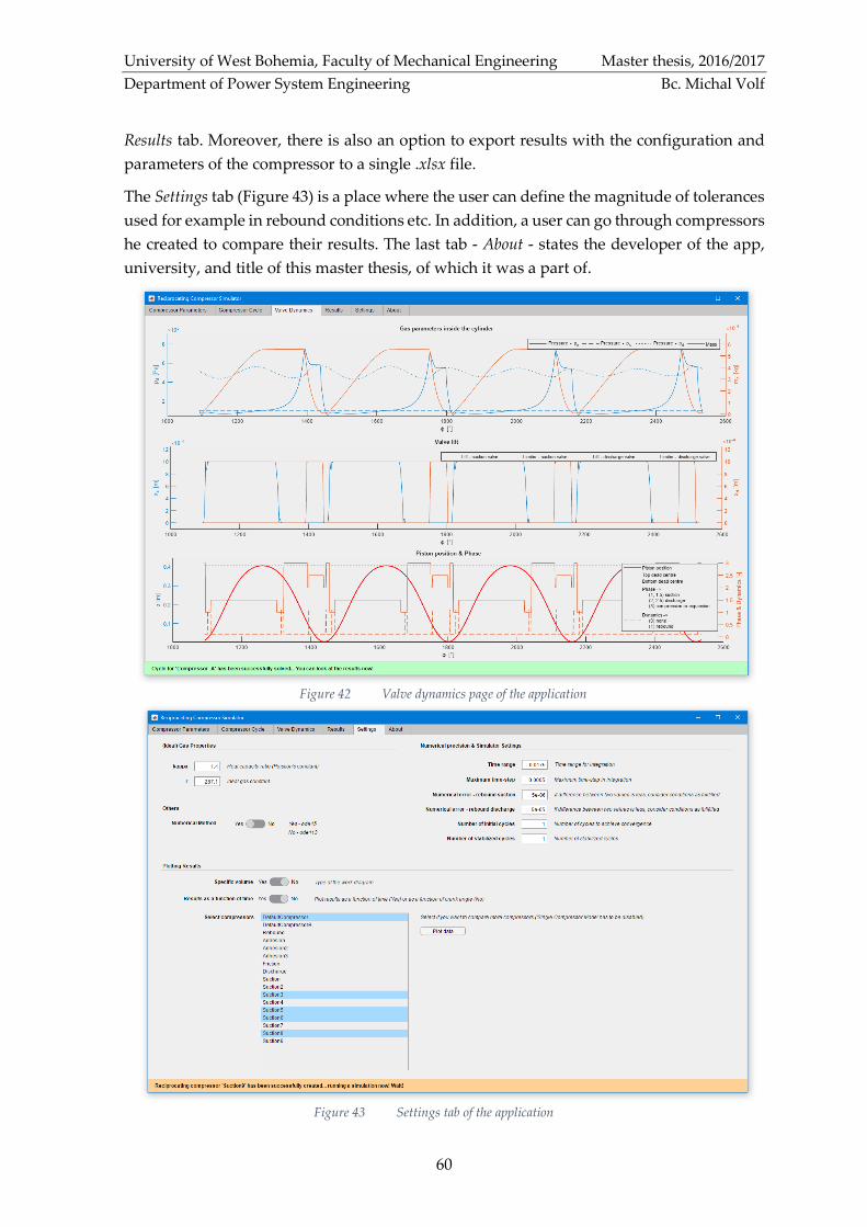
University of West Bohemia, Faculty of Mechanical Engineering Master thesis, 2016/2017
Department of Power System Engineering Bc. Michal Volf
60
Results tab. Moreover, there is also an option to export results with the configuration and
parameters of the compressor to a single .xlsx file.
The Settings tab (Figure 43) is a place where the user can define the magnitude of tolerances
used for example in rebound conditions etc. In addition, a user can go through compressors
he created to compare their results. The last tab - About - states the developer of the app,
university, and title of this master thesis, of which it was a part of.
Figure 42 Valve dynamics page of the application
Figure 43 Settings tab of the application
University of West Bohemia, Faculty of Mechanical Engineering Master thesis, 2016/2017
Department of Power System Engineering Bc. Michal Volf
61
5 Results of the Simulation This chapter presents the results that were obtained with the developed simulation tool
based on the proposed and extensively discussed mathematical model in the previous
chapters of this thesis. At the outset, the results for the predefined valves and the
compressor design will be pursued. Albeit it might segue from the current discourse it
would not be altogether irrelevant to adduce here the deeper insight into the mathematical
model and its dependencies on experimentally-obtained coefficients. Last but definitely not
the least, the different valve parameters are taken into consideration in the final analysis to
perform a study about their influence on valve behavior, while focusing on the individual
valve dynamic effects and their mutual influence on the valve behavior as such.
5.1 Reference Compressor Configuration
The simulation tool offers an overview of compressor valve behavior by evaluating its
dynamics under various working conditions or different valve geometries. In this section,
the results obtained by the simulation tool for a default compressor setup are presented.
This compressor comprises of a cylinder with a diameter of 120 mm with a stroke length of
90 mm. It compresses a gas from 1 bar to 3 bars, the suction valve plate diameter is 36 mm,
whereas the discharge one is 38 mm. The valve port diameters are 34 and 36 mm
respectively. The compressor speed is assumed to be modest with 300 rpm. For other
parameters, see attachment A.
5.1.1 Variables as a Function of the Crank Angle
In the process of the simulation, there are thirty-four parameters, which are constantly
being tracked and recorded. We do not aim to present each of them in the text of this thesis;
however, the interested reader is referred to the enclosed DVD, where he can find the raw
data extracted from the simulation. Among the parameters, which we have chosen to
closely examine here and which are depicted in Figure 44 as a function of the crank angle,
are:
• Valve plate lifts 𝑥𝑠, 𝑥𝑑
• Valve plate velocities 𝑤𝑥𝑠, 𝑤𝑥𝑑
• Cylinder pressure 𝑝𝑐
• Suction chamber pressure 𝑝𝑠
• Discharge chamber pressure 𝑝𝑑
• Piston displacement 𝑧
It should be pointed out, that in each of these plots, there is a crank angle on the x axis. The
initial value is not zero due to the cycles passed prior to achieving a convergent solution
(these are not depicted). Since in automatic valves, the beginning and the end of a
compressor cycle is determined by the force balances on the valve plates, not the piston
position itself, the cycle does not finish or start at the very moment, when the piston reaches
a dead center.

University of West Bohemia, Faculty of Mechanical Engineering Master thesis, 2016/2017
Department of Power System Engineering Bc. Michal Volf
62
Figure 44 Results of the simulation for a default compressor setup

University of West Bohemia, Faculty of Mechanical Engineering Master thesis, 2016/2017
Department of Power System Engineering Bc. Michal Volf
63
Turning our attention to the course of the pressure in the cylinder during the entire
compressor cycle, it can be observed that, at first, as the piston moves towards the bottom
dead center, thus increasing the volume of the cylinder, the pressure decreases until the
pressure difference in front of and behind the valve plate balances the spring and the
adhesion forces and thus allows for the suction valve plate to lift. The gas flowing into the
cylinder causes the pressure inside to slowly, but steadily, rise. Once both the adhesion and
the gas force are overbalanced by the spring force, the suction valve plate returns towards
the seat, letting the compression phase progress. The course of the pressure inside of the
cylinder during both the discharge and the expansion phases can be interpreted in a similar
manner. However, it is worth noticing that due to different valve characteristics chosen in
the simulation, the decrease in cylinder pressure (approx. 0.2 bar lower than 𝑝𝑠0) during
the suction process is not as significant as the increase in cylinder pressure for the discharge
phase (approx. 0.45 bar higher than 𝑝𝑑0 ). Moreover, during the discharge phase, there
seems to be a relatively strong influence of pressure 𝑝𝑐 by the pressure waves in the
discharge plenum chamber, as one can observe that during this phase in question, the
pressure 𝑝𝑐 tends to slide over the 𝑝𝑑. This further supports the importance of a complete
model, rather than a simplified pipe-less one.
Regarding the valves, one can find from the results that the duration of suction phase, i.e.
the period, during which the suction valve plate is not in direct contact with a seat, is
approx. twice as long as the duration of discharge phase. Moreover, one can see the rebound
effect at the moment, when a valve plate strikes against an obstacle, i.e. a seat or a guard.
In the velocity chart, one can observe the jump change of velocity in these moments, as was
previously discussed in chapter 3.4.3.3 regarding valve plate impacts.
The last diagram depicts the piston displacement and its corresponding compressor cycle
phase. Hence, one can observe that the closing of both the suction and the discharge valves,
i.e. the transition to the expansion or compression phases, does not occur at the very
moment of piston movement reversal (as would occur in mechanically operated valves).
This delay is approx. 20° for the suction valve, whereas only 4° for the discharge one. Last
but not least, this chart also provides the information about the beginning and the end of
the bouncing effect (i.e. Impact dynamics).
5.1.2 Indicator Diagram
The indicator diagram of the compressor cycle, i.e. the variation of pressure and volume
within the cylinder, is depicted in Figure 45. Moreover, here the fluctuating pressures in
the adjacent plenum chambers are also shown. It should be emphasized that the areas
below the suction pressure and above the discharge pressure refer to the contributions to
the indicated work resulting from the pressure drops across each of the valves, i.e. these
areas refer to the loss of energy (expressed in the form of indicated suction/discharge valve
work) due to the deviation of real-life valve behavior from that of an idealistic one, as was
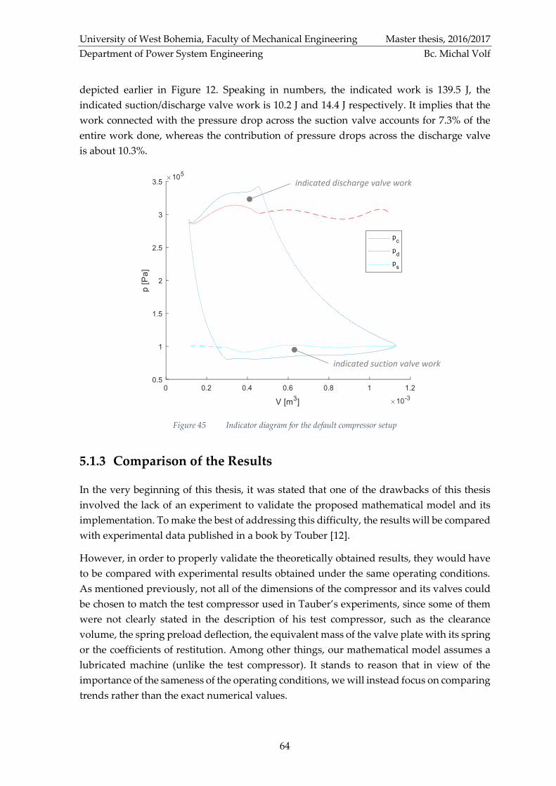
University of West Bohemia, Faculty of Mechanical Engineering Master thesis, 2016/2017
Department of Power System Engineering Bc. Michal Volf
64
depicted earlier in Figure 12. Speaking in numbers, the indicated work is 139.5 J, the
indicated suction/discharge valve work is 10.2 J and 14.4 J respectively. It implies that the
work connected with the pressure drop across the suction valve accounts for 7.3% of the
entire work done, whereas the contribution of pressure drops across the discharge valve
is about 10.3%.
5.1.3 Comparison of the Results
In the very beginning of this thesis, it was stated that one of the drawbacks of this thesis
involved the lack of an experiment to validate the proposed mathematical model and its
implementation. To make the best of addressing this difficulty, the results will be compared
with experimental data published in a book by Touber [12].
However, in order to properly validate the theoretically obtained results, they would have
to be compared with experimental results obtained under the same operating conditions.
As mentioned previously, not all of the dimensions of the compressor and its valves could
be chosen to match the test compressor used in Tauber’s experiments, since some of them
were not clearly stated in the description of his test compressor, such as the clearance
volume, the spring preload deflection, the equivalent mass of the valve plate with its spring
or the coefficients of restitution. Among other things, our mathematical model assumes a
lubricated machine (unlike the test compressor). It stands to reason that in view of the
importance of the sameness of the operating conditions, we will instead focus on comparing
trends rather than the exact numerical values.
indicated discharge valve work
indicated suction valve work
Figure 45 Indicator diagram for the default compressor setup

University of West Bohemia, Faculty of Mechanical Engineering Master thesis, 2016/2017
Department of Power System Engineering Bc. Michal Volf
65
In Figure 46a, one can see the experimental data of cylinder pressure 𝑝𝑐, the suction plenum
chamber 𝑝𝑠 , the discharge plenum chamber 𝑝𝑑 , the suction valve plate lift 𝑥𝑠 and the
discharge valve plate lift 𝑥𝑑. In Figure 46b, one can observe the same quantities extracted
from our simulator tool. As can be seen, there are no noticeable differences in terms of
pressure waveform, however, one can clearly discern the moments when a valve plate
strikes either the guard or seat, and when the valve plate is moving towards the seat. These
inconsistencies presumably result from the differences in parameters regarding the valves
as discussed in the paragraph above. Nonetheless, it can be concluded, based on this
comparison, that the trends are correct.
A related and interesting point to consider here would be the comparison of our results
with other simulators, particularly commercial ones, since it was stated that such a
simulation tool is necessary in the initial stages of valve development. For this purpose, we
obtained an output from a proprietary software used by Dott. Ing. Mario Cozzani Srl
(Figure 47), a company that has been designing and producing valves for reciprocating
compressors since 1946.
In Figure 48, one can see, for comparison purposes, the output from the developed
simulation tool. Bear in mind however, that the used input parameters are the same as with
our previous results, however, in this case the influence of the piping system is omitted as
was done with the output from the commercially developed simulator. Evidently, our
open-source simulator gives very comparable results, at least in terms of trends.
a) b)
Figure 46 Comparison of the experimental and theoretical results

University of West Bohemia, Faculty of Mechanical Engineering Master thesis, 2016/2017
Department of Power System Engineering Bc. Michal Volf
66
5.1.4 Accuracy of the Results
In the previous subchapter, it was concluded that the trends of the valve behavior predicted
by the simulation tool are correct. Regardless of the fact that the only certainty is that the
uncertainties are truly uncertain, let us summarize here the influences on the accuracy of
the output from the simulator tool, which can be divided, based on their origin, as follows:
• Errors resulting from the simplifying assumptions
• Errors present in the input parameters
• Errors resulting from the numerical method used to solve ODEs
The former group, which contains errors resulting from the transition from the physical
model to the mathematical one, was extensively discussed in chapter 3. The second group
refers to errors that can be present in the input parameters, particularly the experimental
coefficients. To examine the dependency of the proposed mathematical model on these
parameters (and thus their accuracy), it is desirable to perform a sensitivity analysis (later
in chapter 5.2.1). Without further discussion, it is reasonable to expect that these errors in
question are the most serious ones, albeit their quantification without a proper experiment
is intractable.
The latter group unites errors that relate to the method of solving the initial condition
problem, i.e. both the numerical method and initial conditions. But how can one decide
whether the method is giving inaccurate results, since the true solution is not known?
Figure 47 Output of valve behavior simulator - Dott. Ing. Mario Cozzani Srl [44]
Figure 48 Output from the developed simulation tool

University of West Bohemia, Faculty of Mechanical Engineering Master thesis, 2016/2017
Department of Power System Engineering Bc. Michal Volf
67
According to Olver [33], a useful and practically employed idea is to integrate the
differential equations using two numerical schemes (of varying orders of accuracy) and
then compare the results. Therefore, in addition to the fourth-order Runge-Kutta method, we
tried the Adams-Bashforth-Moulton predictor-correctors method [36] (of order 1 to 13,
implemented as ode113 in MATLAB). In Figure 49, one can see the p-V diagrams, whereas
in Table 13, there is a comparison of the periodical quantities.
𝑊𝑖[𝐽] 𝑊𝑖𝑣𝑠[𝐽] 𝑊𝑖𝑣𝑑[𝐽] 𝜂𝑣 [%]
Runge-Kutta (ode45) 139.5513 10.2400 14.3785 81.78
Adams-Bashforth-Moulton (ode113) 139.5505 10.2371 14.3651 81.71
Table 13 Comparison of periodical quantities - different ode solvers
It follows that the deviation of the periodical quantities is reasonably small, the variation
being in the hundredths. Furthermore, there are no noticeable deviations in terms of the
trends in p-V diagram and thus it can be concluded that the two solutions are reasonably
close. Hence, it is safe to assume that both methods are giving accurate results.
A slightly different situation arises in terms of the choice of initial conditions at the very
beginning of the integration process, as discussed in chapter 4.3.2.3. Figure 50 depicts the
completed compressor cycles prior to the moment, when the solution is considered to be
convergent. This decision is made on the basis of difference of two successive cycles; if the
difference in pressure in the cylinder does not exceed one thousandth of the discharge
pressure, it is assumed that convergence was achieved.
It can be observed, that more initial cycles are needed in cases, where the influence of the
piping systems is considered (Figure 50a) relative to the second one (Figure 50b), where this
influence is neglected. This concurs well with the statement made earlier that only a rough
estimation of initial conditions is available in the former case.
Figure 49 Comparison of the solution from different ode solvers

University of West Bohemia, Faculty of Mechanical Engineering Master thesis, 2016/2017
Department of Power System Engineering Bc. Michal Volf
68
5.2 Modified Compressor Parameters
5.2.1 Sensitivity Analysis
As the mainstay of the mathematical model in terms of valve behavior, one can consider
the fluid-structure interaction. Recall that the gas force acting on the valve plate is
calculated per a gas coefficient. This coefficient can be obtained experimentally; however,
since we strive for a theoretical approach, we calculate it via an expansion coefficient and a
flow coefficient. The former can be determined theoretically; however, the latter must be
obtained experimentally and so one might consider this substitution of the gas coefficient
to be unbeneficial at first since the gas force does not entirely enough to relinquish the
dependence on experimental coefficients. However, it should be emphasized that the flow
coefficient is required anyway to calculate the mass flow through the valve and so this
substitution helps to reduce the need for further measurements. Moreover, it can provide
us with a valuable insight into the parameters, on which the value of the gas coefficient
mostly depends. For this purpose, we will perform the sensitivity analysis of 𝑐𝑔, which, as
we believe, can help to increase our understanding and intuition of the system.
𝑐𝑔 = (1 + (𝛼𝜖𝜋𝐷𝑣𝑥
𝐴𝑝)
2
)𝐴𝑝
𝐴𝑣−
(𝛼𝜖(𝐴𝑣 − 𝐴𝑝))2
𝐴𝑣𝐴𝑝 (5.2.1)
Figure 50 Compressor cycles prior to convergent solution
a)
b)
convergence
convergence

University of West Bohemia, Faculty of Mechanical Engineering Master thesis, 2016/2017
Department of Power System Engineering Bc. Michal Volf
69
First lets adjust Eq. 5.2.1 by substituting for the areas 𝐴𝑣 =𝜋𝐷𝑣
4
4 and 𝐴𝑝 =
𝜋𝐷𝑝2
4, i.e.:
𝑐𝑔 = (1 + (𝛼𝜖4𝐷𝑣𝑥
𝐷𝑝2 )
2
) (𝐷𝑝
𝐷𝑣)
2
−(𝛼𝜖(𝐷𝑣
2 − 𝐷𝑝2))
2
𝐷𝑣2𝐷𝑝
2 (5.2.2)
Suppose that the function above models the output of a process, where 𝑥 (the valve plate
lift) is the input and 𝐷𝑝, 𝐷𝑣, 𝛼, 𝜖 are models of the system parameters. For the purposes of
analysis, let the normal operating point (NOP) be:
𝑥0 = 1.5, 𝐷𝑝0 = 10, 𝐷𝑣0 = 12, 𝛼0 = 0.6, 𝜖0 = 0.9, (5.2.3)
which produces 𝑐𝑔 ≅ 0.76.
Now let us ask ourselves what is the easiest way to change the value of 𝑐𝑔, i.e. a slight
variation in which parameter will have the biggest impact on the resulting value of 𝑐𝑔? This
sounds a lot like a natural problem for a relative-sensitivity analysis of function 𝑐𝑔 . The
relative-sensitivity functions (the following equations) are formed by multiplying the
partial derivative by the normal value of the parameter and dividing it by the normal value
of the function [37].
𝑆̅𝐷𝑝
𝑐𝑔 =𝜕𝑐𝑔
𝜕𝐷𝑝|
𝑁𝑂𝑃
𝐷𝑝0
𝑐𝑔0= (
2𝐷𝑝0
𝐷𝑣02 −
32(𝑥0𝛼0𝜖0)2
𝐷𝑝03 − (𝛼0𝜖0)2 (
2𝐷𝑝0
𝐷𝑣02 −
2𝐷𝑣02
𝐷𝑝03 ))
𝐷𝑝0
𝑐𝑔0 ≅ 2.12 (5.2.4)
𝑆̅𝐷𝑣
𝑐𝑔 =𝜕𝑐𝑔
𝜕𝐷𝑣|𝑁𝑂𝑃
𝐷𝑣0
𝑐𝑔0= (−
2𝐷𝑝02
𝐷𝑣03 − (𝛼0𝜖0)2 (
2𝐷𝑣0
𝐷𝑝02 −
2𝐷𝑝02
𝐷𝑣03 ))
𝐷𝑣0
𝑐𝑔0≅ −2.40 (5.2.5)
𝑆�̅�
𝑐𝑔 =𝜕𝑐𝑔
𝜕𝛼|
𝑁𝑂𝑃
𝛼0
𝑐𝑔0= (
32𝛼0𝜖02𝑥0
2
𝐷𝑝02 − 2𝛼0𝜖0
2 (𝐷𝑣0
2
𝐷𝑝02 +
𝐷𝑝02
𝐷𝑣02 − 2))
𝛼0
𝑐𝑔0≅ 0.17 (5.2.6)
𝑆�̅�
𝑐𝑔 =𝜕𝑐𝑔
𝜕𝜖|
𝑁𝑂𝑃
𝜖0
𝑐𝑔0= (
32𝜖0𝛼02𝑥0
2
𝐷𝑝02 − 2𝜖0𝛼0
2 (𝐷𝑣0
2
𝐷𝑝02 +
𝐷𝑝02
𝐷𝑣02 − 2))
𝜖0
𝑐𝑔0≅ 0.17 (5.2.7)
𝑆�̅�
𝑐𝑔 =𝜕𝑐𝑔
𝜕𝑥|
𝑁𝑂𝑃
𝑥0
𝑐𝑔0= (
32𝑥0𝛼02𝜖0
2
𝐷𝑝02 )
𝑥0
𝑐𝑔0≅ 0.28 (5.2.8)
These equations give us insight into the behavior of the system only in the case where one
of the parameters is being changed. However, what about the interactions, i.e. how the
system behaves when changing two parameters at the same time? These interaction terms
are obtained by, for instance, the partial derivative of 𝑐𝑔 with respect to 𝑥 containing 𝐷𝑝.
Below are only the non-zero relative-sensitivity functions.
𝑆̅𝑥−𝐷𝑝
𝑐𝑔 =𝜕2𝑐𝑔
𝜕𝑥𝜕𝐷𝑝|
𝑁𝑂𝑃
𝑥0𝐷𝑝0
𝑐𝑔02 = (−
64𝑥0𝛼02𝜖0
2
𝐷𝑝03 )
𝑥0𝐷𝑝0
𝑐𝑔02 ≅ −0.73 (5.2.9)
𝑆�̅�−𝛼
𝑐𝑔 =𝜕2𝑐𝑔
𝜕𝑥𝜕𝛼|𝑁𝑂𝑃
𝑥0𝛼0
𝑐𝑔02 = (
64𝑥0𝛼0𝜖02
𝐷𝑝02 )
𝑥0𝛼0
𝑐𝑔02 ≅ 0.73 (5.2.10)
𝑆�̅�−𝜖
𝑐𝑔 =𝜕2𝑐𝑔
𝜕𝑥𝜕𝜖|
𝑁𝑂𝑃
𝑥0𝜖0
𝑐𝑔02 = (
64𝑥0𝜖0𝛼02
𝐷𝑝02 )
𝑥0𝜖0
𝑐𝑔02 ≅ 0.73 (5.2.11)
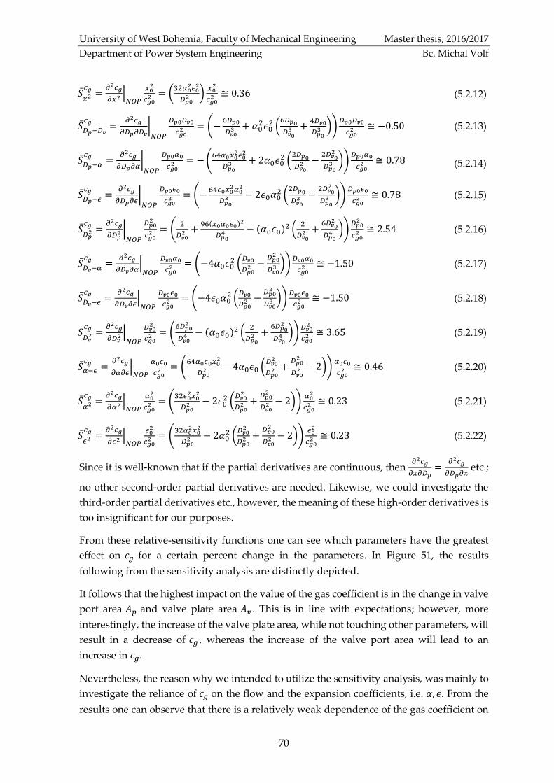
University of West Bohemia, Faculty of Mechanical Engineering Master thesis, 2016/2017
Department of Power System Engineering Bc. Michal Volf
70
𝑆̅𝑥2
𝑐𝑔 =𝜕2𝑐𝑔
𝜕𝑥2 |𝑁𝑂𝑃
𝑥02
𝑐𝑔02 = (
32𝛼02𝜖0
2
𝐷𝑝02 )
𝑥02
𝑐𝑔02 ≅ 0.36 (5.2.12)
𝑆̅𝐷𝑝−𝐷𝑣
𝑐𝑔 =𝜕2𝑐𝑔
𝜕𝐷𝑝𝜕𝐷𝑣|
𝑁𝑂𝑃
𝐷𝑝0𝐷𝑣0
𝑐𝑔02 = (−
6𝐷𝑝0
𝐷𝑣03 + 𝛼0
2𝜖02 (
6𝐷𝑝0
𝐷𝑣03 +
4𝐷𝑣0
𝐷𝑝03 ))
𝐷𝑝0𝐷𝑣0
𝑐𝑔02 ≅ −0.50 (5.2.13)
𝑆̅𝐷𝑝−𝛼
𝑐𝑔 =𝜕2𝑐𝑔
𝜕𝐷𝑝𝜕𝛼|𝑁𝑂𝑃
𝐷𝑝0𝛼0
𝑐𝑔02 = − (
64𝛼0𝑥02𝜖0
2
𝐷𝑝03 + 2𝛼0𝜖0
2 (2𝐷𝑝0
𝐷𝑣02 −
2𝐷𝑣02
𝐷𝑝03 ))
𝐷𝑝0𝛼0
𝑐𝑔02 ≅ 0.78 (5.2.14)
𝑆̅𝐷𝑝−𝜖
𝑐𝑔 =𝜕2𝑐𝑔
𝜕𝐷𝑝𝜕𝜖|
𝑁𝑂𝑃
𝐷𝑝0𝜖0
𝑐𝑔02 = (−
64𝜖0𝑥02𝛼0
2
𝐷𝑝03 − 2𝜖0𝛼0
2 (2𝐷𝑝0
𝐷𝑣02 −
2𝐷𝑣02
𝐷𝑝03 ))
𝐷𝑝0𝜖0
𝑐𝑔02 ≅ 0.78 (5.2.15)
𝑆̅𝐷𝑝
2
𝑐𝑔 =𝜕2𝑐𝑔
𝜕𝐷𝑝2 |
𝑁𝑂𝑃
𝐷𝑝02
𝑐𝑔02 = (
2
𝐷𝑣02 +
96(𝑥0𝛼0𝜖0)2
𝐷𝑝04 − (𝛼0𝜖0)2 (
2
𝐷𝑣02 +
6𝐷𝑣02
𝐷𝑝04 ))
𝐷𝑝02
𝑐𝑔02 ≅ 2.54 (5.2.16)
𝑆̅𝐷𝑣−𝛼
𝑐𝑔 =𝜕2𝑐𝑔
𝜕𝐷𝑣𝜕𝛼|𝑁𝑂𝑃
𝐷𝑣0𝛼0
𝑐𝑔02 = (−4𝛼0𝜖0
2 (𝐷𝑣0
𝐷𝑝02 −
𝐷𝑝02
𝐷𝑣03 ))
𝐷𝑣0𝛼0
𝑐𝑔02 ≅ −1.50 (5.2.17)
𝑆̅𝐷𝑣−𝜖
𝑐𝑔 =𝜕2𝑐𝑔
𝜕𝐷𝑣𝜕𝜖|
𝑁𝑂𝑃
𝐷𝑣0𝜖0
𝑐𝑔02 = (−4𝜖0𝛼0
2 (𝐷𝑣0
𝐷𝑝02 −
𝐷𝑝02
𝐷𝑣03 ))
𝐷𝑣0𝜖0
𝑐𝑔02 ≅ −1.50 (5.2.18)
𝑆̅𝐷𝑣
2
𝑐𝑔 =𝜕2𝑐𝑔
𝜕𝐷𝑣2 |
𝑁𝑂𝑃
𝐷𝑣02
𝑐𝑔02 = (
6𝐷𝑝02
𝐷𝑣04 − (𝛼0𝜖0)2 (
2
𝐷𝑝02 +
6𝐷𝑝02
𝐷𝑣04 ))
𝐷𝑣02
𝑐𝑔02 ≅ 3.65 (5.2.19)
𝑆�̅�−𝜖
𝑐𝑔 =𝜕2𝑐𝑔
𝜕𝛼𝜕𝜖|
𝑁𝑂𝑃
𝛼0𝜖0
𝑐𝑔02 = (
64𝛼0𝜖0𝑥02
𝐷𝑝02 − 4𝛼0𝜖0 (
𝐷𝑣02
𝐷𝑝02 +
𝐷𝑝02
𝐷𝑣02 − 2))
𝛼0𝜖0
𝑐𝑔02 ≅ 0.46 (5.2.20)
𝑆̅𝛼2
𝑐𝑔 =𝜕2𝑐𝑔
𝜕𝛼2 |𝑁𝑂𝑃
𝛼02
𝑐𝑔02 = (
32𝜖02𝑥0
2
𝐷𝑝02 − 2𝜖0
2 (𝐷𝑣0
2
𝐷𝑝02 +
𝐷𝑝02
𝐷𝑣02 − 2))
𝛼02
𝑐𝑔02 ≅ 0.23 (5.2.21)
𝑆̅𝜖2
𝑐𝑔 =𝜕2𝑐𝑔
𝜕𝜖2 |𝑁𝑂𝑃
𝜖02
𝑐𝑔02 = (
32𝛼02𝑥0
2
𝐷𝑝02 − 2𝛼0
2 (𝐷𝑣0
2
𝐷𝑝02 +
𝐷𝑝02
𝐷𝑣02 − 2))
𝜖02
𝑐𝑔02 ≅ 0.23 (5.2.22)
Since it is well-known that if the partial derivatives are continuous, then 𝜕2𝑐𝑔
𝜕𝑥𝜕𝐷𝑝=
𝜕2𝑐𝑔
𝜕𝐷𝑝𝜕𝑥 etc.;
no other second-order partial derivatives are needed. Likewise, we could investigate the
third-order partial derivatives etc., however, the meaning of these high-order derivatives is
too insignificant for our purposes.
From these relative-sensitivity functions one can see which parameters have the greatest
effect on 𝑐𝑔 for a certain percent change in the parameters. In Figure 51, the results
following from the sensitivity analysis are distinctly depicted.
It follows that the highest impact on the value of the gas coefficient is in the change in valve
port area 𝐴𝑝 and valve plate area 𝐴𝑣 . This is in line with expectations; however, more
interestingly, the increase of the valve plate area, while not touching other parameters, will
result in a decrease of 𝑐𝑔 , whereas the increase of the valve port area will lead to an
increase in 𝑐𝑔.
Nevertheless, the reason why we intended to utilize the sensitivity analysis, was mainly to
investigate the reliance of 𝑐𝑔 on the flow and the expansion coefficients, i.e. 𝛼, 𝜖. From the
results one can observe that there is a relatively weak dependence of the gas coefficient on

University of West Bohemia, Faculty of Mechanical Engineering Master thesis, 2016/2017
Department of Power System Engineering Bc. Michal Volf
71
2.12
-2.40
0.17
0.17
0.28
-0.73
0.73
0.73
0.36
-0.50
0.78
0.78
2.54
-1.50
-1.50
3.65
0.46
0.23
0.23𝑆̅𝜖2
𝑐𝑔→
𝑆̅𝛼2
𝑐𝑔→
𝑆�̅�−𝜖
𝑐𝑔→
← 𝑆ത𝐷𝑣−𝜖
𝑐𝑔
← 𝑆ത𝐷𝑣−𝛼
𝑐𝑔
𝑆ത𝐷𝑝
2
𝑐𝑔→
𝑆ത𝐷𝑣
2
𝑐𝑔→
𝑆ത𝐷𝑝−𝜖
𝑐𝑔→
𝑆ത𝐷𝑝−𝛼
𝑐𝑔→
𝑆ത𝑥2
𝑐𝑔→
𝑆ത𝑥−𝜖𝑐𝑔 →
𝑆ത𝑥−𝛼𝑐𝑔 →
𝑆ത𝑥𝑐𝑔 →
𝑆ത𝜖𝑐𝑔 →
𝑆ത𝛼𝑐𝑔 →
← 𝑆ത𝐷𝑣
𝑐𝑔
𝑆ത𝐷𝑝
𝑐𝑔→
← 𝑆ത𝑥−𝐷𝑝
𝑐𝑔
← 𝑆ത𝐷𝑝−𝐷𝑣
𝑐𝑔
𝛼, 𝜖 in comparison to other parameters. This is rather important because, as discussed in
chapter 3.4.2, the expansion coefficient can be determined theoretically and thus the whole
matter of mass flow and fluid-structure interaction as such can be built solely on the flow
coefficient, which, however, is not the parameter influencing the valve behavior the most.
Moreover, recall that this coefficient depends on the geometrical shape of the valve, while
being almost entirely independent of its size. This suggests that regardless of the
semi-empirical approach in modeling the gas force, it does not restrict the applicability of
the model as such.
Figure 51 Sensitivity analysis for the gas coefficient 𝑐𝑔

University of West Bohemia, Faculty of Mechanical Engineering Master thesis, 2016/2017
Department of Power System Engineering Bc. Michal Volf
72
5.2.2 Individual Phenomena Effect
Lets now examine, how the individual phenomena of valve dynamics influence ideal 8
behavior of the valve. For this purpose, each of the charts below depicts an ideal valve plate
movement with its movement influenced by the phenomena in question. The compressor
parameters, in other aspects, correspond to the default ones.
Adhesion
Starting with the adhesion effect (Figure 52), the results correspond to the statement made
earlier, that adhesion delays the valve opening and closing. Speaking in numbers, suction
valve opening is delayed by 2.8°, whereas its closing is delayed only by 0.8°. Regarding the
discharge valve, it can be stated that the delay, due to the stiction, is not as significant in
terms of crank angle, 1.2° or 0.6° for opening and closing respectively.
Friction
As shown in Figure 53, the fluid friction influences the slope of the curve indicating the
stroke of the plate lift during its motion towards either the seat or the limiter, not the
moment, when the valve plate is set in motion as in the previous case. Due to this effect, the
period of opening and closing is lengthened by 3.2° or 4.1° respectively for the suction valve
and 1.4° or 2.1° respectively for the discharge valve.
8 Bear in mind, that by ideal behavior (or movement) it is meant to neglect friction, adhesion, rebound
and pressure pulsations, i.e. the valve plate still moves with a finite velocity, not infinite as it would
in cases of truly idealistic behavior.
Figure 52 Influence of adhesion
Figure 53 Influence of friction

University of West Bohemia, Faculty of Mechanical Engineering Master thesis, 2016/2017
Department of Power System Engineering Bc. Michal Volf
73
Rebound
In Figure 54, one can notice the bouncing effect in the moment when a valve plate strikes
against a limiter or a guard. This collision is modeled as semi-elastic, i.e. it is assumed that
there is some sort of kinetic energy recovery during the collision. The velocity charts show
that the opening of both the suction and discharge valves passes off faster relatively to their
closing, presumably due to the interaction between the valve and its environment (𝑑
𝑑𝑡Δ𝑝).
It is plausible that the nature of the proposed mathematical model could have influenced
the rebound effect, since flow separation at the edges of the valve plate result in turbulent
free jets, in which the energy is dissipated, is not modeled; i.e. it is not postulated that the
potential rebound could be stifled by the resulting low pressure in the air cushion when the
valve tries to move away from the obstacle, especially the guard.
Figure 54 Influence of rebound
A
B
C
D
A B C D

University of West Bohemia, Faculty of Mechanical Engineering Master thesis, 2016/2017
Department of Power System Engineering Bc. Michal Volf
74
Plenum Chambers
It is beyond doubt that one of the reasons of good trend agreement of theoretical results
with experimental ones (chapter 5.1.3) is the presence of pressure pulsations in both the
suction and discharge plenum chambers, despite utilizing the relatively simple
replacement model (i.e. the Helmholtz resonator concept). The comparison of results for
when the pressure pulsations are modeled or not can be observed in Figure 55.
Regarding a deeper breakdown of the concept used to account for pressure pulsations; the
single degree of freedom oscillator consists of a purely inert (mass-like) and purely
compliant (spring-like) element. Therefore, when a piping system is isolated, i.e. a
compressor valve is closed, the gas inside performs free damped oscillations (with a
frequency equal to the natural frequency of the system); however, should the valve be
opened, the oscillations will become forced, since they will be excited by the flowing gas.
The free oscillations are not harmonic, since the governing equations used to describe the
piping systems are not linear. Moreover, from the governing equations one can also
conclude that the frequency of pulsations can be considered to be inversely proportional to
the volume of the plenum chamber; the lower the volume, the higher the frequency (see
Figure 56, where the pressure pulsations in cases with half of the volume of both of the
plenum chambers are depicted).
Figure 55 Influence of piping systems
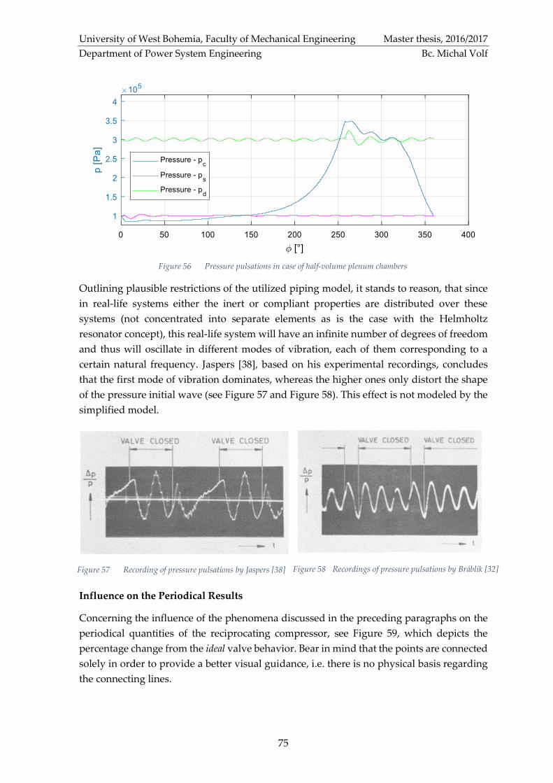
University of West Bohemia, Faculty of Mechanical Engineering Master thesis, 2016/2017
Department of Power System Engineering Bc. Michal Volf
75
Outlining plausible restrictions of the utilized piping model, it stands to reason, that since
in real-life systems either the inert or compliant properties are distributed over these
systems (not concentrated into separate elements as is the case with the Helmholtz
resonator concept), this real-life system will have an infinite number of degrees of freedom
and thus will oscillate in different modes of vibration, each of them corresponding to a
certain natural frequency. Jaspers [38], based on his experimental recordings, concludes
that the first mode of vibration dominates, whereas the higher ones only distort the shape
of the pressure initial wave (see Figure 57 and Figure 58). This effect is not modeled by the
simplified model.
Influence on the Periodical Results
Concerning the influence of the phenomena discussed in the preceding paragraphs on the
periodical quantities of the reciprocating compressor, see Figure 59, which depicts the
percentage change from the ideal valve behavior. Bear in mind that the points are connected
solely in order to provide a better visual guidance, i.e. there is no physical basis regarding
the connecting lines.
Figure 56 Pressure pulsations in case of half-volume plenum chambers
Figure 57 Recording of pressure pulsations by Jaspers [38] Figure 58 Recordings of pressure pulsations by Bráblík [32]
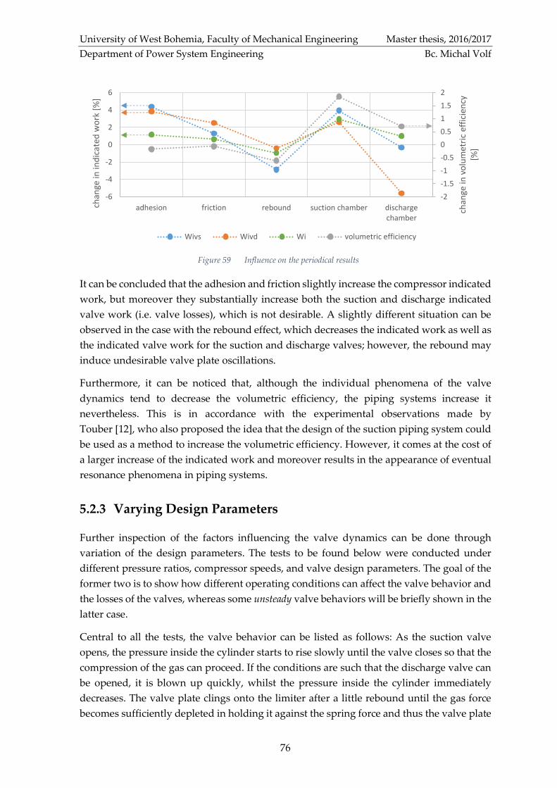
University of West Bohemia, Faculty of Mechanical Engineering Master thesis, 2016/2017
Department of Power System Engineering Bc. Michal Volf
76
It can be concluded that the adhesion and friction slightly increase the compressor indicated
work, but moreover they substantially increase both the suction and discharge indicated
valve work (i.e. valve losses), which is not desirable. A slightly different situation can be
observed in the case with the rebound effect, which decreases the indicated work as well as
the indicated valve work for the suction and discharge valves; however, the rebound may
induce undesirable valve plate oscillations.
Furthermore, it can be noticed that, although the individual phenomena of the valve
dynamics tend to decrease the volumetric efficiency, the piping systems increase it
nevertheless. This is in accordance with the experimental observations made by
Touber [12], who also proposed the idea that the design of the suction piping system could
be used as a method to increase the volumetric efficiency. However, it comes at the cost of
a larger increase of the indicated work and moreover results in the appearance of eventual
resonance phenomena in piping systems.
5.2.3 Varying Design Parameters
Further inspection of the factors influencing the valve dynamics can be done through
variation of the design parameters. The tests to be found below were conducted under
different pressure ratios, compressor speeds, and valve design parameters. The goal of the
former two is to show how different operating conditions can affect the valve behavior and
the losses of the valves, whereas some unsteady valve behaviors will be briefly shown in the
latter case.
Central to all the tests, the valve behavior can be listed as follows: As the suction valve
opens, the pressure inside the cylinder starts to rise slowly until the valve closes so that the
compression of the gas can proceed. If the conditions are such that the discharge valve can
be opened, it is blown up quickly, whilst the pressure inside the cylinder immediately
decreases. The valve plate clings onto the limiter after a little rebound until the gas force
becomes sufficiently depleted in holding it against the spring force and thus the valve plate
Figure 59 Influence on the periodical results
-2
-1.5
-1
-0.5
0
0.5
1
1.5
2
-6
-4
-2
0
2
4
6
adhesion friction rebound suction chamber dischargechamber
chan
ge in
vo
lum
etri
c ef
fici
ency
[%
]
chan
ge in
ind
icat
ed w
ork
[%
]
Wivs Wivd Wi volumetric efficiency

University of West Bohemia, Faculty of Mechanical Engineering Master thesis, 2016/2017
Department of Power System Engineering Bc. Michal Volf
77
will return to the seat. Although the trends of the valve plate movement are basically the
same for all the tests, some details can be noticed.
Valve Movement under Different Discharge Pressures
Suction pressure is kept constantly at 1 bar, while discharge pressure is adjusted
from 3 bars up to 7 bars. Figure 60 depicts p-V diagrams, whereas Figure 61 shows the valve
lift as a function of the crank angle.
One can see from both of the above diagrams that the increasing discharge pressure
shortens the magnitude of the suction and discharge phases, while at the same time it
lengthens both the compression and expansion phases. Careful examination of the valve
movement indicates the higher the discharge pressure is, the higher the impact velocities
for the discharge valve are, whereas in the case of the suction valve the impact velocities
are uninfluenced by the varying discharge pressure (see Figure 62). Moreover, the rebound
process tells us that the discharge valve is blown higher by the higher discharge pressure
-2
-1
0
1
2
3
4
2.5 3 3.5 4 4.5 5 5.5 6 6.5 7 7.5
imp
act
velo
city
[m
/s]
discharge pressure [bar]
suction valve - limiter suction valve - seat discharge valve - limiter discharge valve - seat
Figure 62 Impact velocities - various discharge pressures
detail
detail
Figure 61 Valve lift - various discharge pressures Figure 60 p-V diagrams - various discharge pressures

University of West Bohemia, Faculty of Mechanical Engineering Master thesis, 2016/2017
Department of Power System Engineering Bc. Michal Volf
78
(see Figure 61). In order to be thorough, the lines in the charts below are best-fit linear
trendlines, i.e. they are obtained by utilizing the regression analysis method of least squares.
In Figure 63, the courses of periodical quantities for the various tested discharge pressures
are depicted. It is needless to say that the indicated work rises as the compression ratio rises.
Moreover, it can be observed that the indicated valve work for both the suction and the
discharge valves becomes smaller as the corresponding phase proceeds faster, i.e. as the
discharge pressure increases; however, it is at the cost of a substantial decrease in the
volumetric efficiency.
Valve Movement under Different Compressor Speeds
Through adjusting the frequency of the current, the revolutions are gradually increased
from 300 rpm up to 550 rpm. As shown in Figure 64, the discharging period decreases after
increasing the compressor speed. Also, the impact velocities rise, as can be observed in
Figure 65. Regarding the periodical quantities, see Figure 66.
60%
65%
70%
75%
80%
85%
volu
met
ric
effi
cien
cy [
%]
0
20
40
60
80
100
120
140
160
180
200
0
2
4
6
8
10
12
2.5 3.5 4.5 5.5 6.5 7.5
ind
icat
ed w
ork
[J]
ind
icat
ed v
alve
wo
rk [
J]
discharge pressure [bar]
Wivs Wivd Wivolumetric efficiency
Figure 63 Periodical quantities - various discharge pressures
Figure 64 Valve movement under various compressor speeds

University of West Bohemia, Faculty of Mechanical Engineering Master thesis, 2016/2017
Department of Power System Engineering Bc. Michal Volf
79
Figure 65 Impact velocities - various compressor speeds
Valve Movement for Different Valve Parameters
Since the valve is modeled as a mass-spring system, it goes without saying that such a
system is also potentially an oscillating system, in which the excitation necessary to give
rise to the oscillating behavior of the sealing element is provided by the interaction of the
system with the flow. This phenomenon, known in the corresponding literature as flutter,
is truly undesired behavior since it is a widely-held view that it can result in premature
valve failures [2].
Flutter has been investigated by several researchers, both theoretically and experimentally.
Hence, the interested reader can be referred to the recent literature of Böswirth [13], where
a theoretical model of valve flutter, verified experimentally, is formulated. Even though
that our interest in this thesis is not concerned with an elaboration of unsteady valve
behaviors, it is felt that it would be beneficial to show that the proposed mathematical
-2
-1
0
1
2
3
250 300 350 400 450 500 550 600
imp
act
velo
city
[m
/s]
revolutions [rpm]
suction valve - limiter suction valve - seat discharge valve - limiter discharge valve - seat
70%
73%
76%
79%
82%
85%
88%
volu
met
ric
effi
cien
cy [
%]
0
20
40
60
80
100
120
140
160
180
0
5
10
15
20
25
30
300 350 400 450 500 550
ind
icat
ed w
ork
[J]
ind
icat
ed v
alve
wo
rk [
J]
revolutions [rpm]
Wivs Wivd Wivolumetric efficiency
Figure 66 Periodical quantities - various compressor speeds
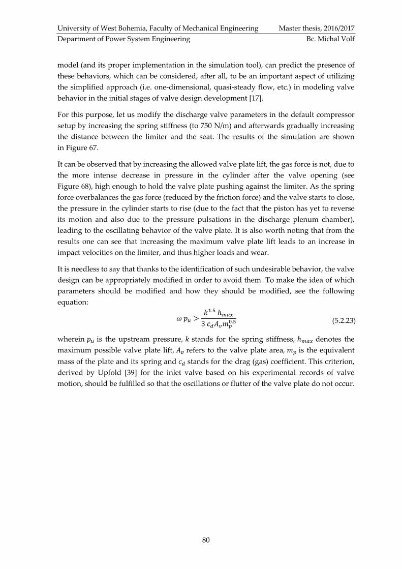
University of West Bohemia, Faculty of Mechanical Engineering Master thesis, 2016/2017
Department of Power System Engineering Bc. Michal Volf
80
model (and its proper implementation in the simulation tool), can predict the presence of
these behaviors, which can be considered, after all, to be an important aspect of utilizing
the simplified approach (i.e. one-dimensional, quasi-steady flow, etc.) in modeling valve
behavior in the initial stages of valve design development [17].
For this purpose, let us modify the discharge valve parameters in the default compressor
setup by increasing the spring stiffness (to 750 N/m) and afterwards gradually increasing
the distance between the limiter and the seat. The results of the simulation are shown
in Figure 67.
It can be observed that by increasing the allowed valve plate lift, the gas force is not, due to
the more intense decrease in pressure in the cylinder after the valve opening (see
Figure 68), high enough to hold the valve plate pushing against the limiter. As the spring
force overbalances the gas force (reduced by the friction force) and the valve starts to close,
the pressure in the cylinder starts to rise (due to the fact that the piston has yet to reverse
its motion and also due to the pressure pulsations in the discharge plenum chamber),
leading to the oscillating behavior of the valve plate. It is also worth noting that from the
results one can see that increasing the maximum valve plate lift leads to an increase in
impact velocities on the limiter, and thus higher loads and wear.
It is needless to say that thanks to the identification of such undesirable behavior, the valve
design can be appropriately modified in order to avoid them. To make the idea of which
parameters should be modified and how they should be modified, see the following
equation:
𝜔 𝑝𝑢 >𝑘1.5 ℎ𝑚𝑎𝑥
3 𝑐𝑑𝐴𝑣𝑚𝑝0.5 (5.2.23)
wherein 𝑝𝑢 is the upstream pressure, 𝑘 stands for the spring stiffness, ℎ𝑚𝑎𝑥 denotes the
maximum possible valve plate lift, 𝐴𝑣 refers to the valve plate area, 𝑚𝑝 is the equivalent
mass of the plate and its spring and 𝑐𝑑 stands for the drag (gas) coefficient. This criterion,
derived by Upfold [39] for the inlet valve based on his experimental records of valve
motion, should be fulfilled so that the oscillations or flutter of the valve plate do not occur.

University of West Bohemia, Faculty of Mechanical Engineering Master thesis, 2016/2017
Department of Power System Engineering Bc. Michal Volf
81
Figure 68 Pressure in the cylinder under various maximum discharge valve lifts – discharge phase
Figure 67 Valve movement under various maximum discharge valve lifts
University of West Bohemia, Faculty of Mechanical Engineering Master thesis, 2016/2017
Department of Power System Engineering Bc. Michal Volf
82
Conclusion
Considering the valves of the reciprocating compressor as a key component highly
influencing the reliability as well as the efficiency of this type of compressor, and
furthermore given the irreplaceability of these machines in applications throughout various
industrial branches, it is imperative that the design of the valves and their behavior is
pursued seriously. First and foremost, this thesis has been devoted to providing an
elaboration of the phenomena by which the valve dynamics is constituted and the
parameters which influence them, whilst the emphasis has been put on their qualitative
assessment.
For the purpose of fulfilling the stated goals, a mathematical model describing the motion
of compressor valves has been proposed. The introduced simplifying assumptions have
been extensively discussed, factoring into their impact on the accuracy of results. This
model has been afterwards implemented into a tool in the commercially available software
known as MATLAB, utilizing the programming paradigm based on objects to maintain the
versatility and customizability of the model. In the final analysis, besides the discussion of
valve behavior under various design parameters, a deeper insight has been gained into the
dependency of the mathematical model on experimentally-obtained coefficients.
Despite the fact that there are some limitations, mainly due to the restriction of the sealing
element dynamics to one-dimension, the assumption of quasi-steady flow, etc. used
heretofore, which do not permit, in the aftermath, the study of effects like unparalleled
collisions or an extensive study of nonstationary behaviors, the model has the potential to
be widely utilized; either in the very early stages of valve design development, or as a
valuable tool to predict quantities, which are hard to measure such as impact velocities etc.
This is also supported by the satisfactory agreement of the trends of valve plate motion with
experimental data borrowed from the cited sources.
The modeling of valve dynamics is still a research subject and thus there are areas, in which
further improvement would be welcomed. As an important matter for further study one
can consider an alternative to the calculation of mass flow through valves on the basis of a
flow coefficient, establishing the variation of the gas force with the flow or by considering
unsteady effects at small valve openings.
University of West Bohemia, Faculty of Mechanical Engineering Master thesis, 2016/2017
Department of Power System Engineering Bc. Michal Volf
References
1. Kompresory. [Online] 2012. [Citace: 12. 11 2016.]
http://kke.zcu.cz/export/sites/kke/about/projekty/enazp/projekty/01_Stavba-a-provoz-
stroju_1-3/1_IUT/002_Kompresory---Kolarcik-a-kol---P3.pdf.
2. Ninković, Dobrivoje and Taranović, Dragan and Pešić, Radivoje. Modelling Valve
Dynamics and Flow in Reciprocating Compressors. [Online] 2013. [Cited: 11 15, 2016.]
http://oaji.net/articles/2014/766-1398015561.pdf.
3. Compressor Valves and Unloaders for Reciprocating Compressors. [Online] 2002. [Cited:
11 12, 2016.] http://d-rco.com/techpapers/tp015.pdf.
4. Howes, Brian and Long, Bryan. Using Simulation of Reciprocating Compressor Valve
Dynamics to Improve Economic Performance. [Online] [Cited: 2 5, 2017.]
http://www.betamachinery.com/assets/pdfs/Technical_Articles/Using_Simulation_of_Reci
procating_Compressor_Valve_Dynamics_to_Improve_Economic_Performance.pdf.
5. Habing, R. A. Flow and Plate Motion in Compressor Valves. [Online] 2005. [Cited: 10 4,
2016.] http://doc.utwente.nl/50744/1/thesis_Habing.pdf. ISBN 90-365-2179-3.
6. Stetefeld, R. Els- und Kalteerzeugungsmaschinen. Stuttgart : s.n., 1901.
7. Hirsch, M. Die Kaltemaschine. Berlin : Springer, 1932.
8. Lanzendörfer, E. Strömungsvorgange und Bewegungsverhaltnisse bei Druckventilen
schnell-laufender Kompressoren. s.l. : Z. VDI 76, 1932.
9. Costagliola, M. The theory of spring-Loaded Valve for Reciprocating Compressor. s.l. :
Journal of Applied Mechanics 17 415-20, 1950.
10. Pereira, Evandro L. L. and Dechamps, Cesar J. and Ribas, Fernando A. Numerical
Analysis of Heat Transfer inside the Cylinder of Reciprocating Compressors in the Presence
of Suction and Discharge Processes. [Online] 2010. [Cited: 10 5, 2016.]
http://docs.lib.purdue.edu/cgi/viewcontent.cgi?article=2994&context=icec.
11. Study of the Effective Flow Area of Compressor Plate Valve . [Online] 1994. [Cited: 11
5, 2016.] http://docs.lib.purdue.edu/cgi/viewcontent.cgi?article=1976&context=icec.
12. Touber, Simon. A Contribution to the Improvement of Compressor Valve Design.
[Online] 1976. [Cited: 9 2016, 10.] http://repository.tudelft.nl/islandora/object/
uuid:4c12fa64-32c6-4fd5-9ebc-e733621c96ac/datastream/OBJ/view.
13. Böswirth, L. Flow Forces and the Tilting of Spring Loaded Valve Plates - Part I.
[Online] 1980. [Cited: 11 8, 2016.] http://docs.lib.purdue.edu/cgi/viewcontent.cgi?
article=1329&context=icec.
14. Tuhovcak, Jan and Hejčík, Jiří and Jícha, Miroslav. Modelling fluid flow in a
reciprocating compressor . [Online] 2015. [Cited: 12 5, 2016.] http://www.epj-
conferences.org/articles/epjconf/pdf/2015/11/epjconf_efm2014_02100.pdf.

University of West Bohemia, Faculty of Mechanical Engineering Master thesis, 2016/2017
Department of Power System Engineering Bc. Michal Volf
15. Experiences with Simulation of Reciprocating Compressor Valve Dynamics. Howes,
Brian and Lin, Leonard and Zacharias, Val. Calgary, Canada : International Pipeline
Conference — Volume 2, ASME1996, 1996. IPC1996-1904.
16. Bloch, Heinz P. and Hoefner, John J. Reciprocating Compressors: Operation &
Maintenance. Houston : Gulf Professional Publishing, 1996. ISBN-0080515940,
9780080515946.
17. Tierean, Mircea Horia and Baltes, Liana Sanda. Design of Valves Used in Reciprocating
Compressors . [Online] [Cited: 11 12, 2016.] ISBN: 978-960-474-140-3.
18. Mechanical Engineering Site. Reciprocating Compressor basic parts. [Online] [Cited:
11 15, 2016.] http://www.mechanicalengineeringsite.com/reciprocating-compressor-basic-
parts/.
19. Burckhardt Poppet Valve™. [Online] Burckhardt Compression AG. [Cited: 2 12, 2017.]
http://www.burckhardtcompression.com/service/components/compressor-valves/poppet/
20. Maclaren, J.F. T. and Kerr, S.V. and Tramschek, A. B. and Sanjines, A. A Model of a
Single Stage Reciprocating Gas Compressor Accounting for Flow Pulsations. [Online]
[Cited:12,7,2016] http://docs.lib.purdue.edu/cgi/viewcontent.cgi?article=1111&context=icec
21. Deviations from Ideal Gas Law Behavior. [Online] Bodner Research Web. [Cited: 2 1,
2017.] http://chemed.chem.purdue.edu/genchem/topicreview/bp/ch4/deviation.php.
22. Ideal Gas Law . [Online] The Engineering ToolBox. [Cited: 2 1, 2017.]
http://www.engineeringtoolbox.com/ideal-gas-law-d_157.html.
23. Tuhovcák, Ján and Hejčík, Jiří and Jícha, Miroslav. Heat Transfer Analysis in the
Cylinder of Reciprocating Compressor. [Online] 2016. [Cited: 12 28, 2016.]
http://docs.lib.purdue.edu/cgi/viewcontent.cgi?article=3408&context=icec.
24. Thermodynamics and Propulsion. Control volume form of the conservation laws .
[Online] Massachusetts Institute of Technology. [Cited: 10 3, 2016.]
http://web.mit.edu/16.unified/www/FALL/thermodynamics/notes/node19.html.
25. Mass and Energy Balance of Unsteady-flow Processes. [Online] [Cited: 10 25, 2016.]
https://ecourses.ou.edu/cgi-bin/ebook.cgi?doc=&topic=th&chap_sec=04.5&page=theory.
26. Anon. Simulation of a reciprocating compressor, Application study (PACE analog
computer). Long Beach, N.J., U.S.A. : Electronic Associates Inc., 1963. 11-4-la.
27. Mechanics Lecture Notes. Notes for lecture 9 and 10: Momentum and Impulse. [Online]
[Cited: 2 8, 2017.] http://www.damtp.cam.ac.uk/user/stcs/courses/mechanics/lecturenotes/
L9_L10.pdf.
28. Müllner, Thomas. Flow Patterns and Valve Dynamics in Multi-Valve Reciprocating
Compressors. [Online] 2015. [Cited: 3 2, 2017.] https://publik.tuwien.ac.at/
files/PubDat_244144.pdf.
University of West Bohemia, Faculty of Mechanical Engineering Master thesis, 2016/2017
Department of Power System Engineering Bc. Michal Volf
29. Pizarro-Recabarren, Rodrigo Adrian and Barbosa, Jader Jr. and Deschamps, Cesar J.
Modeling the Stiction Effect in Automatic Compressor Valves. [Online] 7 16, 2012. [Cited:
12 5, 2016.] http://docs.lib.purdue.edu/cgi/viewcontent.cgi?article=3043&context=icec.
30. Khalifa, H. E. and Liu, X. Analysis of Stiction Effect on the Dynamics of Compressor
Suction Valve. [Online] 1998. [Cited: 12 28, 2016.] http://docs.lib.purdue.edu/cgi/
viewcontent.cgi?article=2220&context=icec.
31. Fleming, J.S. and Tramschek, A.B. and Abdul-Husain, J.M.H. Comparison of Flow
and Pressure Distribution in Simple Valves Using Different Computational Methods.
[Online] 1988. [Cited: 11 28, 2016.] http://docs.lib.purdue.edu/cgi/viewcontent.cgi?
article=1606&context=icec.
32. Bráblík, J. Gas pulsations as a factor affecting operation of automatic valves in
reciprocating compressors. s.l. : International Compressor Conference, Purdue, 1972. p. 188.
33. Olver, J. Nonlinear Ordinary Differential Equations. [Online] 2012. [Cited: 1 10, 2017.]
http://www-users.math.umn.edu/~olver/am_/odz.pdf.
34. ode45. [Online] [Cited: 12 20, 2016.] https://www.mathworks.com/help/matlab/
ref/ode45.html#outputarg_y.
35. Ordinary Differential Equation Solvers ODE23 and ODE45. [Online] [Cited: 4 15, 2017.]
https://blogs.mathworks.com/cleve/2014/05/26/ordinary-differential-equation-solvers-
ode23-and-ode45/#a495083d-5d4a-4fac-afbc-768444430751.
36. Ashino, Ryuichi and Nagase, Michihiro and Vaillancourt, Rémi. Behind and Beyond
the MATLAB ODE Suite. [Online] Division of Mathematical Sciences, Osaka Kyoiku
University, Kashiwara, 1 2000. [Cited: 4 15, 2017.] https://www.wire.tu-
bs.de/docs/lehre/veranstaltungen/uebungen/ode1_ws05/MatlabODESuite.pdf.
37. Smith, Eric D. and Szidarovszky, Ferenc and Karnavas, William J. and Bahill, A.
Terry. Sensitivity Analysis, a Powerful System Validation Technique. [Online] [Cited: 12
27, 2016.] http://citeseerx.ist.psu.edu/viewdoc/download?doi=10.1.1.149.4781&rep=rep1&
type=pdf
38. Special suction lines influencing the volumetric efficiency of reciprocating compressors.
Jaspers, H. A. Madrid : s.n., 1967. Proc. XII Int. Congr. Refrig. Madrid, paper 3.54.
39. Upfold, R.W. Designing Compressor Valves to Avoid Flutter. [Online] 1972. [Cited: 4
20, 2017.] pp. 400-406..
40. Compressor Valves. [Online] CPI. [Cited: 11 5, 2016.] http://c-p-i.com/en/compressor-
valves/.
41. Guerra, Christopher J. and Kolodziej, Jason R. A Data-Driven Approach for Condition
Monitoring of Reciprocating Compressor Valves . [Online] [Cited: 10 5, 2016.]
http://gasturbinespower.asmedigitalcollection.asme.org/article.aspx?articleid=1770088.

University of West Bohemia, Faculty of Mechanical Engineering Master thesis, 2016/2017
Department of Power System Engineering Bc. Michal Volf
42. Affonzo, Luis Octavio Amaral. Machinery Failure Analysis Handbook: Sustain Your
Operations and Maximize Uptime. s.l. : Elsevier, 2013. ISBN-9780127999821.
43. Heat and Mass Transfer Technological Center . Fluid Structure interaction . [Online]
Universitat Politècnica de Catalunya, Barcelona. [Cited: 4 2, 2017.]
http://www.cttc.upc.edu/research/node/77.
44. Reciprocating Compressor Valves: Design. [Online] Dott. Ing. Mario Cozzani Srl.
[Cited: 4 14, 2017.] http://www.cozzani.com/capabilities/design/.

University of West Bohemia, Faculty of Mechanical Engineering Master thesis, 2016/2017
Department of Power System Engineering Bc. Michal Volf
A-1
A Default Compressor Setup
Here we state the default input parameters, with which the simulation tool was tested and
which were used in the qualitative comparison of our results with others. Since we did not
find the exact parameters needed for our simulator in any of the cited conference
proceedings, from which we used the experimental results, we employed data from various
other sources to arrive at admissible values.
Ideal gas
heat capacity ratio 𝜅 1.4 [−]
ideal gas constant 𝑟 287.1 [𝐽𝑘𝑔−1𝐾−1]
Crank mechanism
connecting rod length 𝐿 0.18 [𝑚]
cylinder diameter 𝐷𝑐 0.12 [𝑚]
clearance length 𝑧0 0.01 [𝑚]
angular velocity of the crankshaft 𝜔 31.4 [𝑟𝑎𝑑 𝑠−1]
radius of the crankshaft 𝑅 0.045 [𝑚]
Suction valve
spring preload deflection 𝑥0,𝑠 0.01 [𝑚]
maximum valve plate lift ℎ𝑠 0.00125 [𝑚]
spring stiffness 𝑘𝑠 13 [𝑁𝑚−1]
mass (plate with equivalent of spring) 𝑚𝑠 0.015 [𝑘𝑔]
valve plate diameter 𝐷𝑣,𝑠 0.036 [𝑚]
valve port diameter 𝐷𝑝,𝑠 0.034 [𝑚]
coefficient of restitution 𝑐𝑟,𝑠 0.5 [−]
friction coefficient 𝑐𝑓,𝑠 3.2 [𝑁𝑠𝑚−1]
flow coefficient 𝛼𝑠 0.65 [−]
Discharge valve
spring preload deflection 𝑥0,𝑑 0.005 [𝑚]
maximum valve plate lift ℎ𝑑 0.00125 [𝑚]
spring stiffness 𝑘𝑑 125 [𝑁𝑚−1]
mass (plate with equivalent of spring) 𝑚𝑑 0.018 [𝑘𝑔]
valve plate diameter 𝐷𝑣,𝑑 0.038 [𝑚]
valve port diameter 𝐷𝑝,𝑑 0.036 [𝑚]
coefficient of restitution 𝑐𝑟,𝑑 0.4 [−]
friction coefficient 𝑐𝑓,𝑑 2.8 [𝑁𝑠𝑚−1]
flow coefficient 𝛼𝑑 0.7 [−]

University of West Bohemia, Faculty of Mechanical Engineering Master thesis, 2016/2017
Department of Power System Engineering Bc. Michal Volf
A-2
Suction piping system
static pressure in steady-state reservoir 𝑝𝑠0 100000 [𝑃𝑎]
static temperature in the reservoir 𝑇𝑠0 293.15 [𝐾]
volume of the suction chamber 𝑉𝑠 0.0008 [𝑚3]
effective length of the suction pipe 𝐿𝑠 1 [𝑚]
effective cross-sectional area of the pipe 𝐴𝑠 0.0003 [𝑚2]
loss coefficient in the suction pipe 𝜉𝑠 1 [−]
Discharge piping system
static pressure in steady-state reservoir 𝑝𝑑0 300000 [𝑃𝑎]
static temperature in the reservoir 𝑇𝑑0 350 [𝐾]
volume of the discharge chamber 𝑉𝑑 0.002 [𝑚3]
effective length of the discharge pipe 𝐿𝑑 1 [𝑚]
effective cross-sectional area of the pipe 𝐴𝑑 0.00035 [𝑚2]
loss coefficient in the discharge pipe 𝜉𝑑 1 [−]
Adhesion
surface tension 𝛾𝐿𝐺 0.012 [𝑁𝑚−1]
meniscus contact angle 𝛽 7.5 [°]
oil film thickness ℎ𝑓𝑖𝑙𝑚 5 ∙ 10−7 [𝑚]
The values of the variables pertaining to the suction and discharge piping systems are
chosen from the source [12]. The variables relating to adhesion are chosen in accordance
with [29]. Regarding the variables, which refer to the crank mechanism and valves, they are
mainly chosen according to the source [12]. The clearance length is derived from the
source [14]. Among the values, for which we decided to use estimated ones and for which
we could not find in any cited source are the preload deflection for the spring and loss
coefficients in the pipes.
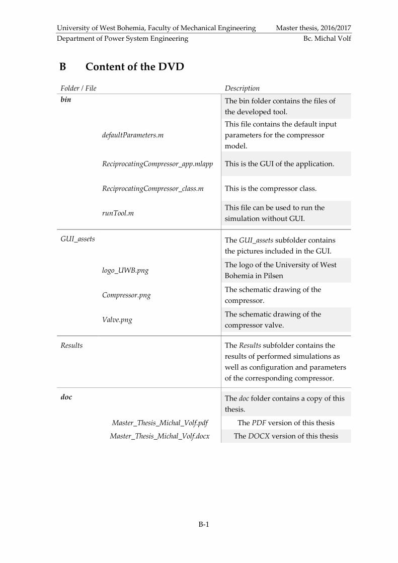
University of West Bohemia, Faculty of Mechanical Engineering Master thesis, 2016/2017
Department of Power System Engineering Bc. Michal Volf
B-1
B Content of the DVD
Folder / File Description
bin The bin folder contains the files of
the developed tool.
defaultParameters.m
This file contains the default input
parameters for the compressor
model.
ReciprocatingCompressor_app.mlapp This is the GUI of the application.
ReciprocatingCompressor_class.m This is the compressor class.
runTool.m This file can be used to run the
simulation without GUI.
GUI_assets
The GUI_assets subfolder contains
the pictures included in the GUI.
logo_UWB.png The logo of the University of West
Bohemia in Pilsen
Compressor.png The schematic drawing of the
compressor.
Valve.png The schematic drawing of the
compressor valve.
Results
The Results subfolder contains the
results of performed simulations as
well as configuration and parameters
of the corresponding compressor.
doc The doc folder contains a copy of this
thesis.
Master_Thesis_Michal_Volf.pdf The PDF version of this thesis
Master_Thesis_Michal_Volf.docx The DOCX version of this thesis