A steady-state analysis of the 'microbial loop' in stratified ... apNA. Phytoplankton and...

Vol. 59: 1-17, 1990 1 MARINE ECOLOGY PROGRESS SERIES Mar. Ecol. Prog. Ser.

Published January 11

A steady-state analysis of the 'microbial loop' in stratified systems

Arnold H. Taylor, Ian Joint

Plymouth Marine Laboratory, Prospect Place, West Hoe, Plymouth PLl 3DH, United Kingdom

ABSTRACT. Steady state solutions are presented for a simple model of the surface mixed layer, which contains the components of the 'microbial loop', namely phytoplankton, picophytoplankton, bacterioplankton, microzooplankton, dissolved organic carbon, detritus, nitrate and ammonia. This system is assumed to be in equilibrium with the larger grazers present at any time, which are represented as an external mortality function. The model also allows for dissolved organic nitrogen consumption by bacteria, and self-grazing and mixotrophy of the microzooplankton. The model steady states are always stable. The solution shows a number of general properties; for example, biomass of each individual component depends only on total nitrogen concentration below the mixed layer, not whether the nitrogen is in the form of nitrate or ammonia. Standing stocks and production rates from the model are compared with summer observations from the Celtic Sea and Porcupine Sea Bight. The agreement is good and suggests that the system is often not far from equilibrium. A sensitivity analysis of the model is included. The effect of varying the mixing across the pycnocline is investigated; more intense mixing results in the large phytoplankton population increasing at the expense of picophytoplankton, microzooplankton and DOC. The change from phytoplankton to picophytoplankton dominance at low mixing occurs even though the same physiological parameters are used for both size fractions. The F-ratio falls abruptly at low mixing rates. Estimates of microbial food web efficiency made with this model show that bacteria are not important, a result confirmed by excluding bacteria from the system. The model therefore does not support the 'microbial loop' hypothesis. The model solutions and parameter values are presented in full in 3 appendices.

INTRODUCTION

Our perception of the functioning of the pelagic food web has changed dramatically in the last 15 yr. In the 'classical' view, such as that modelled by Steele (1974), bacteria were considered only as decomposers of faecal material In the benthos. However, with the introduction of new techniques it is now clear that the biomass and activity of all microbes is much greater than was previously assumed. Picophytoplankton are recognised to be important primary producers in many regions of the world's ocean (Joint 1986, Waterbury et al. 1986); heterotrophic bacteria are postulated to utilize more than 50 % of primary production (Hagstrom et al. 1988); and the role of protozoa is being increasingly examined (Fenchel 1986). This current interest in the role of autotrophic and heterotrophic microbes in the sea has lead to suggestions that there is a separate flow of energy through the microbial components of the food web; Azam et al. (1983) hypothesized that a 'microbial loop' existed within pelagic systems, in which organic

O Inter-Research/Printed in F. R. Germany

matter derived from phytoplankton was utilized by heterotrophic bacteria, which were then grazed by protozoa. The purpose of this paper is to examine interactions within the 'microbial loop' by means of a steady state model.

There have been several recent models which have included microbial components of the food web (Pace et al. 1984, Bratbak & Thingstad 1985, Fasham 1985, Frost 1987). The approach taken in this paper differs from these in that it concentrates on analysis of steady- states. The assumption of an approximate state of equilibrium is frequently made when network analysis techniques are used (Wulf et al. 1987), with an additional condition of linearity often being applied (Michaels & Silver 1988, Ducklow in press); analysis of the kind presented here can provide criteria by which the validity of these assunlptions can be observation- ally assessed. When the system is in the general vicinity of equilibrium, the analysis may give insight into how sensitivity to individual parameters arises, and, in so far as the system is trying to attain an equilibrium

2 Mar. Ecol. Prog. Ser. 59: 1-17, 1990

configuration, may indicate aspects of the time-dependent dynamics. In a fully time-dependent model the requirement for detailed initial conditions, which are difficult to obtain experimentally, can only be avoided by constructing a n ecosystem that is sufficiently general to simulate all seasons of the year (and a wide geographical region if advection is important). Steady- state models are a n alternative tool which may some- times circumvent this complexity. They give algebraic solutions which can be used to estimate values for poorly known parameters from observational data.

The purpose of this paper is to examine the differences in functioning of picophytoplankton and other phytoplankton within the pelagic ecosystem. The model is described in the next section and the properties of its steady-states in that following. Three appendices contain the details of these calculations and of the parameter values used. The ecological significance of the model output is then discussed. In particular, we look at the importance of the microbial loop and the significance of detritus in nutrient regeneration.

THE MODEL

The model (Fig. 1) to be used consists of a surface mixed layer with the following state variables: phytoplankton (P), picophytoplankton (p), free bacteria (B), microzooplankton (z), metabolisable dissolved organic

Fig. l. The model. Single arrows indicate the flows of carbon and nitrogen in the model ecosystem. Double arrows show the exchanges through the bottom of the mixed layer. Phyto. is phytoplankton > l pm, picophyto. is phytoplankton 1 pm. microzoo, is microzooplankton and DOC/N is metabolisable

dissolved organic carbodnitrogen

carbon 'DOC' (D), nitrate (N) , ammonia (A), and detritus (DT). Phytoplankton are considered to be all photosynthetic organisms greater than l Ctm and picophytoplankton are those smaller than 1 pm. The term microzooplankton is used to describe the grazers of picophytoplankton and bacteria; we therefore exclude from this group juvenile stages of macrozooplankton and large protozoa which are not capable of feeding on bacterial-size particles. The bacterial component is assumed to be free-living organisms utilising only dissolved organic carbon. The detritus fraction excludes large particles which sink quickly out of the system.

In formulating and analysing this system 3 assumptions are used:

(1) The system is assumed to be approximately in a steady-state balance with the larger grazers (copepods, etc.) that are present at any time. These grazers can therefore be parameterised as an externally imposed mortality.

(2) A summer situation is assumed; the 2 species of phytoplankton are nitrogen-limited and the bacteria are limited by DOC.

(3) The 2 phytoplankton species have the same half- saturation constants for the uptake of nitrogen. Given the lack of data on nutrient uptake by different size phytoplankton cells in natural assemblages this is a reasonable first assumption which considerably simplifies the mathematical calculations. This assumption is applied to the basic model; however, additional calculations without this restriction will also be described (Tables 1 and 2).

The 8 equations describing the temporal variation of the state variables are:

Taylor & Joint: Analysis of the microbial loop 3

Each coefficient a, describes a rate of transfer between state variables. Thus, a,,, is the constant representing the rate of ammonia (A) production resulting from microzooplankton (z) grazing in picophytoplankton (p). The subscript T is used to represent detritus. In a similar way each coefficient m, (e.g. mDp) is a transfer or loss associated with externally imposed mortality representing natural mortality and grazing by macrograzers. Each parameter v, (e.g. vp) is the loss rate from the mixed layer due to sinking, and is therefore equal to the appropnate sinking speed divided by the depth of the mixed layer. The constant k is the rate of turbulent exchange through the bottom of the surface layer and has dimensions of [TIME]-'. The equations assume that the phytoplankton, picophytoplankton, microzooplankton and detritus are all absent below the mixed layer while nitrate, ammonia, DOC and detritus have the constant concentrations No, A,, D, and DTo, respectively.

The main processes encompassed by these equations are described below.

The phytoplankton equations, Eqs. (1.1, 1.2). These consider phytoplankton growth, and losses due to grazing, sinking and turbulence. Light limitation in the lower part of the mixed layer is incorporated into a p ~ * and apNA. Phytoplankton and picophytoplankton can utilise ammonia and nitrate. Nitrogen limitation is represented by:

with Q, = (N/NH)/(l + N/NH + A/AH) and Q, = (MAH)/ (1 + N/NH + A/AH), NH and AH being half-saturation constants for nitrate and ammonia, respectively [for a discussion of how alternative nutrient sources should be combined see Harris (1974) and Legovic (in press)].

apNA and are defined in the same way. The bacterial equation, Eq. (1.3). Thls describes bac-

terial growth, and losses due to grazing, sinking and turbulent mixing out of the surface layer. DOC limitation is represented by:

where DH is a half-saturation constant. The microzooplankton equation, Eq. (1.4). The

growth rate of microzooplankton is assumed to be pro- portional to the concentrations of the 4 food sources: picophytoplankton, bacteria, detritus and microzooplankton. Losses occur due to grazing, sinking, turbulent mlxing and cannibalism. In the self-grazing term, a, is the difference between the growth rate arising from grazing of microzooplankton, aZg, and the rate of consun~ption of microzooplankton, a,,.

The DOC equation, Eq. (1.5). The first 2 terms describe leakage of DOC during phytoplankton growth and the third term the uptake of DOC by bacterial

growth. The remaining terms treat production of DOC during grazing ('sloppy feeding'), DOC production by breakdown of detritus, and the turbulent transport of DOC.

The nitrate equation, Eq. (1.6). Nitrate uptake by the 2 classes of phytoplankton and by the bacteria, and the transport of nitrate from depth, are the processes considered.

The ammonia equation, Eq. (1.7). Uptake of ammonia by the 2 classes of phytoplankton and by the bacteria, and mixing through the bottom of the mixed layer, are treated as in the nitrate equation. The remaining terms all treat the excretion of ammonia by both kinds of grazers feeding on each phytoplankton species, bacteria, detritus and microzooplankton.

The detritus equation, Eq. (1.8). Detritus (faecal pel- lets) is produced in the course of all grazing (i.e. grazing by microzooplankton and external grazers). It is lost by means of the processes in the first set of brackets; that is, sinking, mixing, grazing by microzooplankton and larger grazers, and breakdown by attached bacteria. The constant mT encapsulates both the effects of larger grazers and of attached bacteria.

The solutions which follow are steady-states for whlch:

dP/dt = dp/dt = dB/dt = dz/dt = dD/dt = dN/dt = dA/dt = dDT/dt = 0

SOLUTIONS

The steady-state solution to (1.1) is:

and so the extent of nitrogen limitation is entirely independent of the behavior of the other species in the system. Eq. (1.2) determines the n~icrozooplankton abundance:

z increases with @,NA. When the picophytoplankton have the same half-saturation constants for nitrogen, so

that @ ~ N A = QNA:

If the growth rate of the picophytoplankton in the absence of nitrogen limitation (apNA) is greater than that of the phytoplankton (aPNA), the abundance of microzooplankton will increase linearly with the mixing coefficient (k). If this is not the case a positive value for z will only be possible if k is not too large. For changes that do not affect the parameters in the picophytoplankton equation the microzooplankton abundance increases with the concentration of dissolved inorganic nitrogen.

4 Mar Ecol. Prog. Ser 59: 1-17, 1990

Eq. (1.3) determines the concentration of DOC:

Decreasing the half-saturation constants for nitrogen of the picophytoplankton increases QD and the concentration of DOC. When @pNa = @NA.

If aBZ(apNA/apNA + l ) /apz - 1 > 0 then will increase linearly with k (as will D when D DH), otherwise @D

will decrease with k. For changes that do not influence the bacterial equation the concentration of DOC increases with the abundance of microzooplankton.

Eq. (1.4) provides a relationship between p, B and DT:

Thus, if by changing any of the parameters in Eqs. (1.1) to (1.3) or (1.5) to (1.8) that do not affect those in (2.4), i.e. that do not change the efficiencies with which grazed carbon is converted to microzooplankton carbon, a change is caused in any of p, B or DT, there must be a compensatory change in the remainder of these variables; e.g. if B and DT go up then p will reduce. In the absence of any 2 of these variables, the third will increase linearly with k and will be independent of the nutrient recycling processes. It follows from (2.4) that consumption of detritus by microzooplankton results in a reduction of the standing stocks of picophytoplankton and bacteria. Eq. (2.4) provides an upper limit for the variables p, B and DT that is independent of all parameters that are not present in this equation. Thus, for example,

With the parameter values in Appendix C, and values of the mixing coefficient, k , of 0.01 to 0.1 m d-l , this upper limit is frequently 10 to 20 mg C m-3 and always less than 100 mg C m-3. Increasing the mixing coefficient raises this limit by about 50 Yo. Because the phytoplankton are not constrained to reach a common equi- libnum with their grazers but are only controlled by nutrient supply, they are not limited and dominate the autotrophs at high mixing rates.

The relationships (2.1) to (2.4) do not depend on how much of the primary production, or of the material that is grazed, is converted into nutrients or detritus. They are also independent of the concentrations of the nutrients below the mixed layer (i.e. No, A, and D,).

Eqs. (2.1) to (2.4) will also apply if the mortalities mp, m, and m ~ , or the sinking rates v, and v,, or the turbulent mixing rate k change with time; providing the parameter values in these equations are considered

to be time averages over a sufficiently long time interval. Levins (1979) and Puccia & Levins (1985) show that, if a variable x(t) is bounded and non-zero over a time interval r, the expectations of dx/dt and (l/x)dx/dt over this interval tend to zero as r becomes large; the expectation of any function f(x) being defined by:

Calculating the expectations of (l/P)dP/dt, (l/p)dp/dt, (l/B)dB/dt and (l/z)dz/dt using (1.1) to (1.4) than leads to Eqs. (2.1) to (2.4) but with mp, m,, mB, vp, vp, vs and k replaced by their expectations.

The complete steady-state solution of (1.1) to (1.8) is given in Appendix A. A property of the solution is that the abundances of the phytoplankton, the picophytoplankton, the bacteria and the detritus all depend linearly on the deep nutrient and detntus concentrations No, A,, D, and DTo. Providing the nitrogen concentrations in the mixed layer are much less than No+ A,, the solutions for P, p, B and DT are independent of the half-saturation constants for nitrate and ammonia uptake and depend only on the total concentration of dissolved nitrogen below the mixed layer, not on whether it is in the form of nitrate or ammonia. Further, nitrogen uptake of bacteria always appears in the solutions as the sum of the bacterial consumption of nitrogen and ammonia, i.e. a A D B + a N ~ ~ , so that the values of P, p , B and DT are unaffected by whether the bacteria take up nitrate or ammonia preferentially.

The solutions in Appendix A can only be applied easily if QpNa and QtNu can be directly calculated from @NA. For most of the calculations to be described it will be assumed that the half-saturation constants for nitrate and ammonia uptake are the same for all the autotrophs, so that QpNA = QzNA =

When the 2 half-saturation constants of the picophytoplankton are each a certain fraction B of those for the phytoplankton and the limitations of nitrate and ammonia are combined as described for Eqs. 1.1 and 1.2, QpNH and QNA are related by:

Whenever the equation is used it is assumed that QzNA = that is, the microzooplankton and picophytoplankton have the same half-saturation constants for nitrogen uptake.

A significant property of the solutions is that the standing stocks and production rates are independent of the incident irradiance and of the extinction coefficient of the water unless the 2 species of phytoplankton have different physiological responses to light or nutrients. This occurs because Eq. (2.1) ensures that aPNA$NA, and hence ap~ , \QNA, will not depend on the irradiance (providing a p N ~ = ~ P N A X a constant that is independent of the incident light); that is the concen-


tration of dissolved nitrogen is adjusted to compensate for any change in production due to a change in the light regime. The solution also contains the terms ~ N A P Q N A , ~ N A ~ @ N A , ~ D P @ N A and ~ D ~ Q N A in which the effects of irradiance might appear but these will each be equal to aPNAQNA multiplied by an expression that does not contain the light intensity. The insensitivity to light of a l-layer system is the reason that a 2-layer response occurs when the thermocline is added to the system (Taylor et al. 1986, Taylor 1988). Of course, it is likely that the 2 phytoplankton groups will differ in their response to irradiance and nutrients, but then the effects of changing light intensity on the standing stocks will be determined by these differences and it wd1 be necessary to have a good estimate of what these differences are.

A similar result could apply between bacteria and DOC as Eq. (2.3) constrains aBD@D to be a constant. Thus, if a B ~ were to change (e.g. in response to changing temperature) the DOC concentration will adjust to compensate for this change and the standing stocks will not alter. However, it is to be expected that temperature will have a wider influence than just on the growth of bacteria.

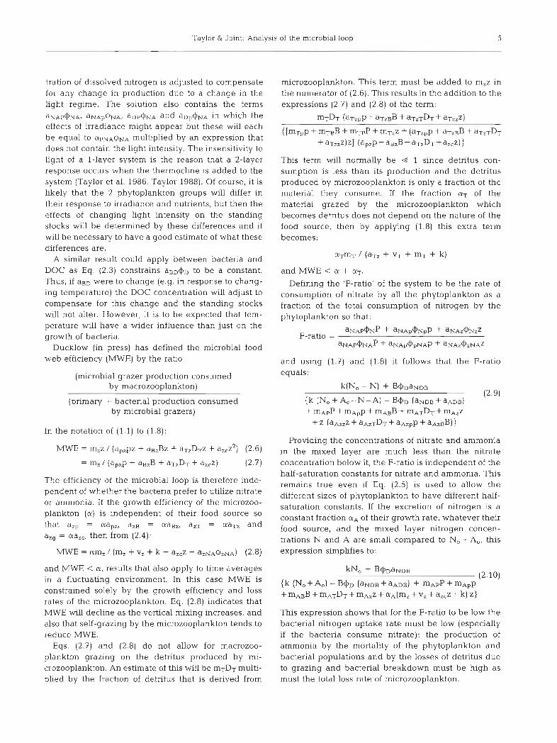
Ducklow (in press) has defined the microbial food web efficiency (MWE) by the ratio

(microbial grazer production consumed by macrozooplankton)

(primary t bacterial production consumed by microbial grazers)

In the notation of (1.1) to (1.8):

The efficiency of the microbial loop is therefore independent of whether the bacteria prefer to utilize nitrate or ammonia. If the growth efficiency of the microzooplankton (a) is independent of their food source so that a,, = &apz, azB = &agZ, a z ~ = aaTz and a,, = aa,,, then from (2.4):

and MWE < a, results that also apply to time averages in a fluctuating environment. In this case MWE is constrained solely by the growth efficiency and loss rates of the microzooplankton. Eq. (2.8) indicates that MWE will decline as the vertical mixing increases, and also that self-grazing by the microzooplankton tends to reduce MWE.

Eqs. (2.7) and (2.8) do not allow for macrozooplankton grazing on the detritus produced by microzooplankton. An estimate of this will be mTDT multiplied by the fraction of detritus that is derived from

microzooplankton. This term must be added to m,z in the numerator of (2.6). This results in the addition to the expressions (2.7) and (2.8) of the term:

~ T D T ( ~ T Z D P + ~ T Z B B + ~ T Z T D T + ~ T Z Z Z )

This term will normally be 4 1 since detritus consumption is less than its production and the detritus produced by microzooplankton is only a fraction of the material they consume. If the fraction &T of the material grazed by the microzooplankton which becomes detritus does not depend on the nature of the food source, then by applying (1.8) this extra term becomes:

and MWE < LY + aT.

Defining the 'F-ratio' of the system to be the rate of consumption of nitrate by all the phytoplankton as a fraction of the total consumption of nitrogen by the phytoplankton so that:

and using (1.7) and (1.8) it follows that the F-ratio equals:

k(N0 - N) + W D ~ N D B {k (No + Ao-N-A) - B@D ( ~ N D B + ~ A D B )

(2.9)

f mApP + m ~ , p + mABB f mATDT + ~ A , Z

+ Z ( ~ A ~ Z Z + ~ A Z T D T + ~ A Z ~ P f ~ A Z B B ) )

Providing the concentrations of nitrate and ammonia in the mixed layer are much less than the nitrate concentration below it, the F-ratio is independent of the half-saturation constants for nitrate and ammonia. This remains true even if Eq. (2.5) is used to allow the different sizes of phytoplankton to have different half- saturation constants. If the excretion of nitrogen is a constant fraction cuA of their growth rate, whatever their food source, and the mixed layer nitrogen concentrations N and A are small compared to No + A,, this expression simplifies to:

This expression shows that for the F-ratio to b e low the bacterial nitrogen uptake rate must be low (especially if the bacteria consume nitrate): the production of ammonia by the mortality of the phytoplankton and bacterial populations and by the losses of detritus due to grazing and bacterial breakdown must be high as must the total loss rate of microzooplankton.

6 Mar Ecol. Prog. Ser 59: 1-17, 1990

MODEL RESULTS

Appendix A describes the solutions of the model which were evaluated using the parameter values listed in Appendix C; the methods used to assign them are summarised in Appendix B. Unless indi- cated, all the calculations assume that the half-saturation constants for nitrogen uptake by the picophytoplankton and the microzooplankton (if used) are the same as those of the phytoplankton.

Fig. 2 shows the magnitudes of the state variables obtained when different values were employed for the coefficient (k) describing the turbulent mixing at the bottom of the mixed-layer Calculations using even larger values of the mixing coefficient lead to nitrate concentrations that are too large for the phytoplankton to be nitrogen-limited and are not consistent with model assumptions. As the stratification gets weaker and there is more mixing across the bottom of the mlxed-layer, there is an increased abundance of phytoplankton, bacteria, detritus and nitrate, together with some decrease in the picophytoplankton. Thus picophytoplankton dominate at low mixing rates, as is frequently observed in oceanic regions (Joint 1986); this result from the model is obtained without impos- ing differences in physiological parameters for the 2 size fractions.

Over most of the range of the mixing coefficient the ammonia concentration stays roughly constant while that of the nitrate increases linearly. This behaviour is fundamental to the system and occurs even if the model includes only phytoplankton, nitrate and ammonia. When the distribution of the carbon pool between its components is examined by

comparing high and low values of the mixing coefficient (Fig. 3) it is seen that, as the proportion of phytoplankton is raised by increasing the mixing, the shares of all the constituents except for bacteria and detritus are substantially reduced (by a factor of 3 or 4 ) . Similarly, the stock of nitrogen (Fig. 4 ) in the phytoplankton grows at the expense of those in the picophytoplankton, microzooplankton, ammonia and DON (estimated by dividing the DOC concentration by the carbonhitrogen ratio for phytoplankton), while those in the bacteria and detritus remain much more constant.

Vertically integrated production rates can be calculated from the model by multiplying the production rate per unit volume by the depth of the mixed-layer. The integrated production rates (Fig. 5) show variations with turbulent mixing that are similar to those of the standing stocks (Fig. 2). For the parameter values that have been employed the production rates for DOC and detritus tend to be numerically equal. The proportion of inorganic nitrogen consumed as nitrate (F-ratio) shows a particularly non-linear response to changes in the vertical mixing coefficient; reductions of the mixing are accompanied by a steadily increasing proportion of the nitrogen consumed as ammonia but at the lowest mixing rates the switch-over from nitrate to ammonia is quite sharp. This curve is the result of a n abrupt replacement of nitrate by ammonla as the mixlng rate is reduced.

Calculations of Ducklow's microbial food web efficiency (MWE, Eqs. 2.6, 2.7) using the standard model parameters (i.e. Fig. 2) give values of 5 to 10°/i, depending on the rate of mixing which suggests that the microbial loop has little influence on higher

Mixing coefficient (/day)

E - Bacteria -- Micmzoo

Mixing coefficient (/day) Mixing coefficient (/day)

A------ I Ammonia

o ! I I I l 0 -' 0.0 ', 1 I I I

0.00 0.02 0.04 0.06 0.08 0.10 0.00 0.02 0.04 0.06 0.08 0.10 0.00 0.02 0.04 0.06 0.08 0.10 Mixing coefficient (/day) Mixing coeffic~ent (/day) Mixing coefficient (/day)

Fig 2. Variation of the equilibrium values of the state-variables with the rate of vertical mixlng


Fig. 3. Percentage of total standing stock of carbon that is in different compartments with low vertical mixing (k = 0.01 d l ) and with high vertical mixing (k = 0.11 d ) . Total standing stock of carbon is given for each

mixing rate

% C (low mixing) 7o C (high mixing)

Detritus

Total carbon = 53.8 (mgC/m3) Total carbon = 219.1 (mgC/m3)

ZN ( low mixing) %N (high mixing)

Fig. 4. Percentage of total standing stock of nitrogen that is in different compartments with low vertical mixing ( k = 0.01 d- ') and with high vertical mixing ( k = 0.11 d- ' ) . Total standing stock of nitrogen is given for each

mixing rate Total nitrogen = 0.9 (mmol/m3) Total nitrogen = 4.1 (mmol/m3)

- Phyto production -- Picophyto production -- 0.00 0.02 0.04 0.06 0.08 0.10


8 Fig. 5. Effect of variation of the verti- 2- cal mixing coefficient on the rate of production of carbon in different com-

-DOC production partments and on the F-ratio (the -- Detritol production

fraction of inorganic nitrogen taken up by all sizes of the phytoplankton as

0 ! , 0.00 0.02 0.04 0.06 0.08 0.10

nitrate) Mixing coefficient (/day)

E 60- /---- - Bocteriol production 20 - - Microzoo production

0- 0.00 0.02 0.04 0.06 0.08 0.10


0.0 0.00 0.02 0.04 0.06 0.08 0.10


8 Mar Ecol. Prog. Ser. 59: 1-17. 1990

Phytoplanktan Nitrate Detritus

E 3 1 0 0 -

P -with bacteria 0.2 - -with bacteria -with bacteria --no bacteria --no bacteria --no bacteria

0 I I I I 0.0 I I I l I 0 I I

0.00 0.02 0.04 0.06 0.08 0.10 0.00 0.02 0.04 0.06 0.08 0.10 0.00 0.02 0.04 0.06 0.08 0.10 Mixing coefficient (/day) Mixing coefficient (/day) Mixing coefficient (/day)

Picophytoplankton Ammonia F-Ratio

0 I 0.0 ' 0.0 I 0.00 0.02 0.04 0.06 0.08 0.10 0.00 0.02 0.04 0.06 0.08 0.10 0.00 0.02 0.04 0.06 0.08 0.10

Mixing coefficient (/day) Mixing coefficient (/day) Mixing coefficient (/day)

------ 12 - -C----

- ------------

E 4 - E l,. 0.2 -

Fig. 6. Effect of variation of the vertical mixing coefficient on the equilibrium values of the state variables and on the F-ratio, when there are no bacteria in the system (broken line). For comparison, the results of Fig. 2 are also shotvn (solid line)

2 -

Phyioplankton Nitrate Bacteria

P 2 - / -with detritus 0.2 - l - / -with detritus -- no detritus -- no detritus -- no detritus

-with bacteria --no bacteria

0 1 7 I l I I I I

0.00 0.02 0.04 0.06 0.08 0.10 0 . 0 4 OJ-

0.00 0.02 0.04 0.06 0.08 0.10 0.00 0.02 0.04 0.06 0.08 0.10 Mixing coefficient (/day) M~xing coefficient (/day) M~x~ng coeffic~ent (/day)

Picophytoplankton Ammonia F-Ratio

-with bacteria --no bacteria

-with bacteria -- no bacteria

Fig. 7 Effect of variation of the vertical mixing coefficient on the equilibrium values of the state variables and on the F-ratio, when detritus is not retained m the system (broken line). For comparison, the results of Fig. 2 are also shown (solid line)

trophic levels. The importance of the microbial loop in the system is further examined by comparing the solutions shown in Fig. 2 with those obtained when bacteria are not present in the system (DOC produced is assumed to disappear from the system) Because the microzooplankton are forced to shift some of their grazing from bacteria to the picophytoplankton, these are especially sensitive to the absence of bacteria; a larger stock of picophytoplankton is needed to sustain

$::::F- -with detritus --no detritus

I l I 1

12 - 10 -

E m

a; \

p 4 -

2 - 0 ,

the microzooplarlkton population. The larger numbers of picophytoplankton are associated with smaller stocks of the phytoplankton (about 20%) and less detritus. Even though the bacteria have been assumed to consume only ammonia and DON, and no nitrate, thelr presence still leads to an Increase in ammonia at the expense of nitrate. This is a consequence of the bacterial production of ammonia from DON. Fig. 6 indicates that the impact of the microbial loop on the

0.00 0.02 0.04 0.06 0.08 0.10 0.00 0.02 0.04 0.06 0.08 0.10 0.00 0.02 0.04 0.06 0.08 0.10 Mixing coefficient (/day) Mixrng coefficient (/day) Mixing coefficient (/day)

-------------Cc

, e 0 . ? - E E 1 / L

0.2 - -with detritus --no detritus

I I l I 0.0

-with detritus -- no detritus

I I , l I 0.0

Taylor & Joint: Analys~s of the microbial loop 9

Phytoplankton + Plcophytoplankton * Bac te r i a

O t +o

*-+--+ - - - - 4- "

I I I I I I I I I

2 8 2 9 3 0 1 2 3 4 5 6 June July

B Phytoplankton + Picophytoplankton 9 Bac te r i a

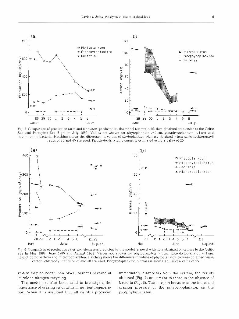
Fig. 8. Comparison of production rates and biomasses predicted by the model (arrows) with data obtained on a cruise to the Celtic Sea and Porcupine Sea Bight in July 1985. Values are shown for phytoplankton > 1 pm, picophytoplankton < 1 Km and heterotrophic bacteria. Hatching shows the difference in values of phytoplankton biornass obtained when carbon: chlorophyll

ratios of 25 and 40 are used. Picophytoplankton biornass is estimated using a value of 25

0

f, P h y t o p l a n k t o n + P i c o p h y t o p l a n k t o n * B a c t e r i a

Mic rozoop lank ton

f + - -A*+ - o - ~ f - ~ ~ ~ * - +- * e o

I I I I I I I I I

M ~ Y June ~ u g u s t May J u n e ~ u g u s t

2 8 2 9 3 0 1 2 3 4 5 6 June Ju ly

Fig 9 Comparison of production rates and biomasses predicted by the model (arrows) with data obtained on cruises to the Celtic Sea in May 1984, June 1986 and August 1982. Values are shown for phytoplankton > l pm, picophytoplankton < l pm, heterotrophic bacteria and microzooplankton. Hatching shows the difference in values of phytoplankton biomass obtained when

carbon: chlorophyll ratios of 25 and 40 are used. Picophytoplankton biomass is estimated using a value of 25

system may be larger than MWE, perhaps because of immediately disappears from the system, the results its role in nitrogen recycling. obtained (Fig. 7) are similar to those in the absence of

The model has also been used to investigate the bacteria (Fig. 6). This is again because of the increased importance of grazing on detritus in nutrient regenera- grazing pressure of the microzooplankton on the tion. When it is assumed that all detritus produced picophytoplankton.

10 Mar. Ecol. Prog. Ser. 59: 1-17, 1990

Table 1. Percentage changes in the values of state variables ~nduced by separately changing each of the parameters listed to the values given. The numbering and units of the parameters arc as in Appendix C. The last column is the change in rate of decay ( d - l ) of the slo~vest decaying mode ( t v e slower decay rate, -ve faster). The first row gives values of the state variables for the control run (mg C m-' but mmol N m ' for A and N). k is 0.01 d- ' Control (1) is the standard parameter set; Control (2) is the same

set but with reduced half-saturation constants for nitrogen uptake by the picophytoplankton

Mode P P B z D N A DT decay

rate

Control (1) (1) Surface irradiance = 300 (5) Light extinction coeff. = 0.20

(22) mp = 0.3 (23, 35) m,, = m~ = 0.3 (30) Max. growth rate of bact. = 2.2 (32) Bacteria take only organic N (32) Bacteria use no organic N (33) Bacteria use NO3 instead of NH, (39, 40 , 41) Grazing rate of microzoo. = 0.025 (41) Grazing rate of microzoo. on detritus = 0.001 (48) m, = 0.3 (49) m ~ . = 0 2 (51) Fraction of microzoo. photosynthesising = 0.2 (53) D T ~ = 2

Half-saturation constants for p and z = 0.3 X those of P l (52) Control (2) -5 33 -3 42 43 - - -5 -

" (l , 52) Surface irradiance = 300 7 -17 2 -20 -21 - 4 - a (22, 52) mp = 0.3 -25 10 4 14 16 - 6 - a (32, 52) Bact. use only org N 46 -5 16 0 0 - 19 -

(51, 52) Fraction of microzoo. phytosynthesising = 0.2 16 -48 -17 0 0 - - -12 -

I Percentage changes from Control (2) I

Comparison with data from the Celtic Sea

The steady states from the model have been compared with observations from a number of cruises in the Celtlc Sea and Porcup~ne Sea Bight obtained during the years 1982 to 1986 by Joint & Pomroy (1983, 1986, 1987) and Joint et al. (1986). In this comparison phytoplankton are considered to be the size-fractions > 1 pm and picophytoplankton as the fraction < 1 Ltm. Pico- phytoplankton is grazed on by the same organisms that graze on bacteria. The appropriate values for the vertical mixing coefficient, k, are not known; this parameter is dependent on the strength of the density stratification and also on the depth of the mixed layer There- fore, the procedure that has been adopted is to use values of this parameter for which the calculated production rates of the phytoplankton match those of the observations. These k values were then used to predict the production rates of the picophytoplankton and ba.c- teria, and the standing stocks of the phytoplankton, picophytoplankton and the bacteria; Fig. 8 shows data on production and biomass for July 1985 and Fig. 9 for cruises in May 1984, June 1986 and August 1982. The predict abundance of the rnicrozoopla.nkton was also

compared (Fig. 9b) with the total abundance of hetero- flagellates and ciliates estimated by Joint & Williams (1985). All the predicted values agree wlth those observed to within a factor of 2 apart from the bacterial production rates and phytoplankton biornass which tend to be higher than observed values. Phytoplankton populations were derived from the chlorophyll a meas- urements using a carbon:chlorophyll ratio of 25.

In August 1983 the F-ratios of the 0.1-0.8 pm fraction and the 5 pm fractions were estimated to be 31 '10 and 22 % respectively (N. J . P. Owens pers. comm.). The corresponding F-ratio from the model calculations was 42 %, the same for each size of phytoplankton.

Sensitivity analysis

The extent to which uncertainties in the values of parameters influence the equilibrium values of the state-variables and fluxes IS summarised in Table 1 (state-variables) and Table 2 (rates of production). The model has over 50 parameters and so the tables only consider those of particular importance. The criteria used in selecting this subset of the parameters were: (1) those parameters

Taylor & Joi.nt: Analysis of the microbial loop 11

Table 2. Percentage changes in the values of vertically integrated production rates induced by separately changing each of the parameters tested to the values given. The numbering and units of the parameters are as in Appendix C. The last column is the pctrcentage change in the F-ratio. The first row gives the values of the production rates for the control run (mg C m-' dC1, but mm01 N m-' d-l for A). k is 0.01 dC1 Control (1) is the standard parameter set; Control (2) is the same set but with reduced half-

saturation constants for nitrogen uptake by the picophytoplankton

P P B z D A DT F-ratio

C:ontrol (1) 153 139 30.4 40.3 2.69 3.69 2.86 0.34 (1) Surface irradiance = 300 -1 1 2 -5 0 -6 -4 -6 1 (5) Light extinction coeff = 0.20 -7 1 -3 0 -3 -2 -4 1

(22) ]mp = 0.3 - 2 99 37 98 3 0 4 3 27 -24 (23, 35) m, = ~n~ = 0.3 -7 -28 -16 -55 -16 -22 -13 18 (30) Max. growth rate of bact. = 2 16 0 0 - 1 0 0 0 0 0 (32) Bacteria use only organic N 33 -7 16 0 16 13 18 -15 (32) Bacteria use no organic N - 25 5 -12 0 -12 -10 -14 15 (33) Bacteria use N o 3 instead of NH, 0 0 0 0 0 0 0 -16 (39, 40, 41) Grazing rate of microzoo. = 0.025 -70 373 122 300 118 156 93 5 1 (41) Grazing rate of microzoo. on detritus = 0.001 - 11 9 29 0 4 -2 5 3 (48) m, = 0.3 -8 53 20 60 18 24 14 -14 (49) m~ = 0.2 - 1 2 0 0 1 0 0 0 (51) Fraction of microzoo. photosynthesising = 0.2 9 -69 -12 -52 -15 -12 -8 9 (53) DTo = 2 0 0 0 0 0 0 0 0

Half-saturation constants for p and z nitrogen 0.3 X those of P

(52) Control (2) -5 87 37 86 30 - 26 -20 " ( l , 52) Surface irradiance = 300 7 -33 -17 -33 -15 - -13 9 " (22, 52) n ~ p = 0.3 23 26 19 2 8 17 - 19 -19 " (32, 52) Bact. use only org. N 46 - 5 16 0 16 - 19 -21 " (51, 52) Fraction of microzoo. phytosynthesising = 0.2 16 -52 -17 -53 -21 - -12 6

Percentage changes from Control (2)

illustrating theoretically predicted behaviour, (2) those for which there is particular uncertainty, (3) those to which the system is especially sensitive, and (4) those indicating the role of processes that have previously been conjectured to be significant. Each parameter was varied across the probable range of its uncertainty.

The main body of each table shows the relative sensitivity of different components of the system to these parameters. Thus, the standing stocks of particulate carbon are almost independent of the surface irradiance, the extinction coefficient, the maxin~um bacterial growth rate or the fraction of inorganic nitro- yen that the bacteria take up as nitrate; results that were all derived from the model solutions. The origin of the slight dependences is discussed in Appendix A (following Eq. A14). The system is only moderately sensitive: to whether the bacteria predominantly use organic or inorganic nitrogen (the response to this parameter being almost linear); to whether the microzooplankton are mixotrophic (the picophytoplankton are the most affected by this); to the externally imposed loss rate of detritus; or to the concentration of detritus below the mixed layer (e.g. Smith et al. 1989).

The system is most sensitive: to the grazing rate of the microzooplankton; to the externally imposed mortality of

the phytoplankton; and, to a lesser extent, to the externally imposed mortalities of the bacteria, picophytoplankton and microzooplankton. These are all parameters whose values are particularly uncertain. Very large values for the externally imposed mortality of the phytoplankton were not used because high values tend tolead to non-limiting ammonia concentrations. Grazing by microzooplankton on detritus was also considered separately; a lower grazing rate than in the standard model may be appropriate because a large fraction of the detritus is unavailable to the microzooplankton. Detritus concentration is the only variable affected appreciably.

An important question to be considered in any steady-state model is 'Will the equilibrium ever be reached?'. This has been examined for the present system by using eigenvalue analysis to determine whether small departures from equilibrium grow or decay (they may be oscillating at the same time). Such perturbations decay for all the model calculations presented here. Therefore the ecosystem will drift towards the equilibrium configuration if it is in its vicinity. Table 1 gives the decay rate of the slowest decaying mode of the system, which has a typical time-scale of 8 d, and uses this to show how variations in different parameters affect stability.

12 Mar. Ecol. Prog. Ser. 59: 1-17, 1990

The lower parts of Tables 1 and 2 show the effects of relaxing the assumption that the different sizes of phytoplankton have the same half-saturation constants for nitrogen. The percentage changes introduced by drop- ping this assumption (using Eq. 2.5), the row 'Control (2) ' in the tables, show that the model is quite sensitive to how little nitrogen the picophytoplankton can take up. The production rates are especially sensitive; those of the picophytoplankton and the bacteria increase to values (249 and 42 mg C d-', respectively) that are inconsistent wlth the observations of Figs. 8 and 9. Agreement could be restored by substantially adjusting some of the other parameters, e .g. lowering the surface irradiance, but this is not attempted here.

The lines following the new control run, 'Control (2)' , show the deviations from these states resulting from varying some of the parameters as previously. The results are generally very similar to those obtained when the different sizes of phytoplankton were given the same Michaelis-Menten constants for nitrogen. However, an exception to this is that the system now shows a response to changes in either light or the extinction coefficient.

The microbial food web efficiency (2.7) was between 5 and 15 % in all the model calculations that have been discussed. It was larger when mixotrophy was occur- ring and smaller when lower half-saturation constants for nitrogen uptake by picophytoplankton were used.

DISCUSSION

In this paper, we have argued that a steady state model is a useful method to study some pelagic processes; but it is important to establish the time scale over which we can assume a quasi-steady state and the dynamics of the biological processes that are modelled. We have confined considerations to the microbial components of the food web. We argue that, although these organisms have short generation times and can respond rapidly to changes in nutrient supply or grazing, these are the very features which are required for the steady state. It is easy to establish a steady state culture of a mlcrobe, or of an assemblage of microbes, but it is very much harder to have steady state growth of a n invertebrate, which may have several life stages with different growth rates. Therefore, it appears entirely appropriate to examine the microbial components of the pelagic food web with a steady state model.

There are other advantages. Steady-state calculations can often be carried out very rapidly lvhich allows a thorough exploration of the parameter space. For instance, the calculations reproduced here are based on several hundred model states. The solutions also

have the potential of being directly applied to observational data. This may not be readily apparent for the solutions given here because they have been made as general as possible, but by leaving out processes considered to be less important simpler equations can be obtained. However, the usefulness of equilibrium states still depends on whether they are likely to occur and on how well they fit the observations.

Determining the growth or decay of small departures from the steady-states showed that the states are almost always stable. Further, subsequent experiments with a time-dependent version of the model have shown that the equilibria frequently are still reached even when the initial states are remote. This stability is surprising at first sight; in general, the more complex a n ecosystem model becomes, the greater is the likeli- hood of one or more non-decaying modes (May 1974). However, Berryman & Millstein (1989) have pointed out that when steady-state analyses are performed on mathematical models based on real data, almost invari- ably stable steady-state behaviour of the modelled systems is observed, suggesting that In real ecosystems there is a preponderance of negative rather than positive feedback processes. The present model would seem to support this.

We have demonstrated that this model gives realistic simulations for most of the microbial components of the pelagic ecosystem: comparisons have been made with experimental data, not only for biomass (Fig. 9) but also for productivity of the microbial system (Fig. 8). We consider such comparisons to be a crucial test of any model. As can be seen from Flgs. 8 and 9, model output is very close to experimental data for all components, except for heterotrophic bacterial production. These experimental data were published by Joint & Pomroy (1983, 1987) and were based on incorporation rates of 3H thymidine. As discussed by Joint & Pomroy (1987), there is a large degree of uncertainty in the factors used to convert bacterial biovolume to biomass, and to relate thymidine uptake to biomass production. Other attempts to model the same data set (Vezina & Platt 1988) have also commented that good agreement of model and field data can only be achieved by using larger conversion factors to estimate productivity than those adopted by Joint & Pomroy (1987). Similarly, conversion of bacterial cell numbers to bacterial carbon would require larger values of the carbon: biomass ratio; but as discussed by Jolnt & Pomroy (1987), this can soon result in conversion factors which produce cells with impossibly high specific gravity. There appears to be too much uncertainty in the estimation of both bacterial biomass and productivity for a critical comparison of model output with field data. Similar uncertainty exists over the most appropriate carbon chlorophyll conversion factor for phytoplankton. We

Taylor & Joint: Analys~s of the microb~al loop 13

have taken a conservative value of 25 : 1 for the carbon. chlorophyll ratio; this gives good agreement between field and model data for picoplankton, but agreement for the larger phytoplankton is improved if this ratio 1s increased. This suggests that picoplankton may have a lower carbon: chlorophyll ratio than other phytoplankton; we have no data to test this prediction.

Another suggestive result from the model is con- stancy of the percentage of the total carbon pool in bacterial biomass and detritus; this contrasts w ~ t h larger variations in the percentages in microzooplankton, picoplankton and DOC. Similar results are also found for the nitrogen pool. This is a prediction of the model that might be testable with data from different regions.

Finally, this study has implications for the 'microbial loop' hypothesis (Azam et al. 1983). which suggests transfer of carbon from bacteria and protozoa to higher trophic levels. The results of this model show that, although rates of carbon assimilation and respiration are high within the 'microbial loop', only a small fraction of the carbon is transferred to higher trophic levevls and the loop does not have a large influence on the recycling of nitrogen. Ducklow et al. (1986), in a study of microbial processes in a mesocosm, found no evidence that carbon assimilated by bacteria could be a significant food source for larger organisms. The results of this model also fail to support the 'microbial loop' hypothesis. The estimates of microbial food web efficiency made with this model show that bacteria are not important; this result is confirmed by model manipula- tion experiments which remove bacteria from the model (Fig. 6). The model supports the conclusion of Ducklow et al. (1986) that heterotrophic bacteria appear to act as a sink for carbon in pelagic food webs; if bacteria are not responsible for the transfer of energy to higher trophic levels, we must examine again the basic premise of the 'microbial loop' hypothesis.

Acknowledgements. This work forms part of Laboratory Research Project 2 of the Plymouth Marine Laboratory, a component of the UK Natural Environment Research Council. We thank John Stephens for very able assistance with com- puting.

APPENDIX A: MODEL SOLUTIONS

Steady-state solutions for @NA, Z , and I$, have been given In Eqs. (2.1) to (2.3). The detritus equation (1.8) expresses DT ln terms of P, p and B

in which hT is the net specific loss rate for detritus, i.e.

Each term in (Al ) is positive and so AT must also be positive or DT will be negative. I f (A l ) is divided throughout by DT it can

be seen that (P/DT) > 1 can only occur if mTp < h, That is, the abundance of the phytoplankton can only be greater than that of the detntus ]fits specific rate of conversion to detritus is less than the net speclfic loss rate of the detritus. The converse is also true so that if mTp > AT then (P/DT) < 1. Similar results hold for (B/DT) and (zaTZR+ mTB)/)LT, and for @/DT) and (zaTzp + ~ T , ) ~ T -

When (Al ) is substituted into (2.4) an equation relating B, P and p results:

hT, is the product of the net spec~fic loss rate for detntus and the total specific loss rate of the microzooplankton:

PB and y, are given by: BB = az~(aTzBz + ~ T B ) + h a z u

By substituting in the DOC Eq. (1.5) using (A1 to A3) a linear equation in the unknowns P and p is obtained. A second linear equation in P and p can be obtained by adding the nitrate equation to that of ammonia, substituting QNA = QN + @ A and then using (A1 to A3). Solving this pair of simultaneous equations gives solutions for P and p.

Cp, CC and jp are constants obtained from the DOC equation:

and tp, Ep and 5, are constants derived from the nitrate and ammonia equations:

These equations also contain the unknown nitrate and ammonia concentrations N and A. However, as these are each much less than the total source concentration (No+ A,) they

Mar. Ecol. Prog. Ser. 59: 1-17, 1990

can be set to zero as a first approximation (the errors are about 10% for the cases shown here). The calculated values of N and A can be used to improve the estimates, a procedure that has been adopted in all the model calculations. If N o t A, is much larger than the half-saturation concentration for nitrogen uptake the additional dependences introduced Into the solutions because of these extra terms will be small. When P and p have been calculated using (A7) and (A8), the bacterial abundance can be obtained from (A3) and DT from (Al).

Providing the different sizes of autotrophs have the same values of NH and AH, the dissolved nitrate concentration N can be derived by substituting 4 1 ~ = (N/NH)/(l + N/NH + A/AH) in the nitrate equatlon (1.6) and C$, = (A/AH)/(l + N/NH + MAH) in the ammonia equation (1.7). When A is eliminated between the resulting equations, a cubic equation in N is obtained which can be solved numerically. The ammonia concentration can then be obtained from:

When bacteria and DOC are not included in the system the solutions can also be obtained from the above set of equations, setting B = 0 where necessary. However, (A9) to (A14) are replaced by:

<C = - {[(a, - ~ T Z T + a ~ d z + m~ + vz + mz - a,D, - @zNAazh4 + V T ] ~ - [(VZ + - + ~ N A ~ ~ N A ) ( ~ T ~ T - a ~ z ) - v ~ a , - m ~ a ~ + a Z ~ m ~ , J z - [(~TZT - a ~ ~ ) a , + ~ , T ~ T ~ ~ I Z ~

f (V, + mz - $ ' ~ N A ~ ~ N A ) ~ T + v ~ V z + V~ - V ~ @ z ~ ~ a r ~ ~ + k2)

APPENDIX B: TRANSFER COEFFICIENTS

Phytoplankton production (Pr) is assumed to be related to light intensity (I) by:

Pr = Pro (I/Ik) / [ l + ( I&)]

in which Ik is the half-saturation light intensity and Pro is the maximum production. If 1 declines with depth (X) according to:

then the average production rate (Tpr) through the surface layer of thickness h is:

h

Tpr = ( l / h ) l Pr dx 0

= Pro log, {(l + Io/Ik) / [ l + Ioexp(-eh)/I,] ) / (eh)

where I , is the surface irradiance. apN, and apNA are each set equal to T,,, substituting the

appropnate values for Ik and the appropriate maximum specific growth rates for Pro.

aDp = a p ~ ~ X fract~on of phytoplan.kton carbon production leaked as DOC

aDP = aPNA X fraction of picophytoplankton carbon production leaked as DOC

aNAp = apNA X 0.071393 / C : N ratio for phytoplankton

aNAP = apNA X 0.071393 / C : N ratio for picophytoplankton

r n p is the externally imposed mortality rate for phytoplankton

m, is the externally imposed mortality rate for picophytoplankton

m ~ p = m, X fraction of phytoplankton externally ~mposed mortality that becomes DOC

mDP = m, X fraction of all picophytoplankton mortality (natural and from grazing) that becomes DOC

mAp = rnp X 0.071393 X fraction of dead phytoplankton nitrogen that becomes ammonia / C : N ratio for phytoplankton

mAp = m, X 0.071393 X fraction of dead picophytoplankton nitrogen that becomes ammonia / C : N ratio for picophytoplankton

m ~ p = mp X fraction of phytoplankton externally imposed mortality becoming detritus

m ~ , = m, X fraction of all picophytoplankton mortality (natural and from grazing) becoming detritus

a B ~ is the maximum specific growth rate of bacteria

a~~ = as,, X DOC consumed per unit of bacterial carbon produced

~ N D B = a ~ , X 0.071393 X fraction of bacterial N obtained from inorganic N X fraction of inorganic N consumed that is nitrate/ C : N ratio for bacteria aAos = aeo X 0.071393 X UBN / C : N ratio for bacteria

UBN is the net uptake rate of bacteria which is:

UBN = (fraction of bacterial N obtained from inorganic N X

fraction of inorganic N consumed that is ammonia) - (fraction of bacterial N obtained from organic N X fraction of DON consumed by bacteria that is excreted)

mB 1s the externally imposed mortality rate for bacteria

moB = me X fraction externally imposed bacterial mortality becoming DOC

mAs = mB X 0.071393 X fraction of dead bacterial nitrogen becoming ammonia / C : N rati.0 for bacteri.a

mw = mB X fraction of externally imposed bacterial mortality becoming detritus

a,, is the fraction of picophytoplankton biomass grazed per unlt time by one unit of microzooplankton

a ~ , is the fraction of bacterial biomass grazed per unlt time by one unit of microzooplankton

a ~ , is the fraction of detrital biornass grazed per unit time by one unit of microzooplankton

a,? = a,, X efficiency of conversion of phytoplankton carbon to m~crozooplankton carbon

a , ~ = aB, X efficiency of conversion of bacterial carbon to microzooplankton carbon

aZT = a ~ , X efficiency of conversion of detrital carbon to microzooplankton carbon

aZNA = apNA X fraction of microzooplankton that are autotrophic

aD, = a , ~ , X fraction of p~cophytoplankton carbon leaked as DOC

~ N A , = a , ~ , x 0.071393 / C : N ratio for picoph.ytoplankton

a,,, = a,, X fraction of all picophytoplankton mortality (natural and from grazing) that becomes DOC

a h n = a ~ , x fraction of all picophytoplankton mortality (natural and from grazing] that becomes DOC

~ D , T = a ~ , X fraction of grazed detritus that becomes DOC

Tavlor & Joint: Analysis of the microbial loop 15

a*.,, = a,, X 0.071393 X fraction of dead picophytoplankton nitrogen that becomes ammonia / C : N ratio for picophytoplankton a A z ~ = a,-, X 0.071393 X fraction of consumed detritus nitrogen that becomes ammonia / C : N rat10 for detritus

a-,, = a,,, X fraction of all picophytoplankton mortality (natural and from grazing) becoming detritus

a.,.,, = a,, X fraction of all bacterial mortality (natural and from grazing) becoming detritus

~ T , T = a ~ , X fraction of grazed detritus becoming detritus m, is the externally imposed mortality rate for microzooplankton m,, = m, X 0.071393 x fraction of all microzooplankton mortality (natural and from grazing) becoming ammonia / C : N ratio for microzooplankton

m ~ , = m, X fraction of microzooplankton mortality (natural and from grazing) becomlng detritus

a,, = a,, X ratio of the rate of m~crozooplankton grazlng microzooplankton : rate of microzooplankton grazing bacteria

a,, = aZs X ratio of the rate of microzooplankton grazing microzooplankton . rate of microzooplankton grazing bacteria

a, = a,, - a,,, a.\,, = a , , ~ X ratio of the rate of microzooplankton grazlng niicrozooplankton . rate of microzooplankton grazing bacteria

aTz, = aT,, X ratio of the rate of microzooplankton grazing microzooplankton : rate of microzooplankton grazing bacteria

m~ is the rate of detntus consumption by the macrograzers and by attached bacteria m ~ , = m, X fraction of detritus loss breaking down to DOC

mnr = mT X 0.071393 x fraction of consumed detritus nitrogen that becomes ammonia / C : N ratio for detritus

APPENDIX C: PARAMETER VALUES

The parameter values used in the standard run of the model are given below. The model was also used to examine the effect of changing some parameter values; In these cases, the alternative values are shown in brackets. The numbering of parameters corresponds to that in Tables 1 and 2.

(1) Mean surface irradiance (I,) 700 (300) btE m-' S- '

(2) Half saturation for llght limited growth ( I k ) 4 5 b ~ ~ m - 2 s ' (Jolnt & Pomroy 1986)

(3) Half saturation constant for phytoplankton growth on nitrate 0.2 umol I - ' (Carpenter & Guillard 1971)

(4) Half saturation constant for phytoplankton growth on ammonia 0. l lcmol l - l (Koike et a1 1983)

(5) Light extinction coefficient ( E )

0.15 (0.20) m (Jordan &Joint 1983) (6) Depth of mixed layer (h)

30 m (Joint & Pomroy 1983) (7) Coeff. of mixing between mixed and bottom layers

0.10 to 0.11 m d-l (8) Nlti-ate concentration below mixed layer (No)

6.0 ~tmol I-' (Joint & Pomroy 1983) (9) Ammonia concentration below mixed layer (A,)

0 pm01 l-' (This is an assumption) (10) DOC concentration below mixed layer

0 mg C m-'

(This is assumed to be 0 since DOC is considered only as DOC produced a s a consequence of the model and does not include a large pool of refractory DOC) Maximum specific growth rate of phytoplankton 0.70 d-l (Banse 1982) blaximum speclfic growth rate of picophytoplankton 1 74 d - ' (Banse 1982) Slnking rate of phytoplankton (vl>) 1.5 d - ' (Bienfang 1980) Sinking rate of picophytoplankton (v 0 m d- '

p! (Takahashi & Bienfang 1983)

Sinking rate of microzooplankton ( v , ) 0 m d-l (Takahashi & Bienfang 1983) Mean sinking rate of detritus (vT) 1 m d-' (Bienfang 1980) Fraction of phytoplankton carbon production leaked as DOC 0.1 (Sharp 1977) Fraction of picophytoplankton carbon production leaked as DOC 0.1 (Sharp 1977) C : N ratio of phytoplankton Assuming that the Redfield ratio applies 5.6 (wt : wt) (Redfleld 1934) C : N ratio of picophytoplankton Assuming that the Redfield ratio applies 5.6 (wt: wt) (Redfield 1934) C : N ratio of heterotrophic bacteria 4.5 (wt: wt) (Goldman et al. 1987) Externally ~mposed mortal~ty rate for phytoplankton (mp)

0.2 (0.3) d - ' (This is an assumed value) Externally imposed mortality rate for picophytoplankton (m,) 0.1 (0.3) d-' (Johnson et al. 1982) Fraction of externally imposed mortality of phytoplankton which becomes DOC 0.1 (This is an assumed value) Fraction of picophytoplankton mortality (natural and from grazing) that becomes DOC 0.1 (This is an assumed value) Fraction of dead phytoplankton nitrogen that becomes ammonia 0.5 (Corner & Davies 197 1) Fraction of dead picophytoplankton nitrogen that becomes ammonia 0 5 (Assumed to be same as for phytoplankton) Fraction of externally imposed mortality on phytoplankton which becomes detritus 0.25 (This is a n assumed value) Fraction of externally imposed mortality in picophytoplankton which becomes detritus 0 25 (This is an assumed value) Maximum specific growth rate of heterotrophc bacteria 4.18 (2.181 d ' (Smits & Riemann 1988) DOC consumed per unit of bacterial carbon produced 2.5 mg C (mg bacterial C)- ' d-' (Newell e t al. 1981) Fraction of bacterial nitrogen obtained from inorganic nitrogen 0.5 (0.0 and 1.0) (This is an assumed value) Fraction of bacterial inorganic nitrogen demand which is nitrate 0 (1.0) (Assuming that dissimilatory utilization of nitrate does not occur in pelagic systems and that ammonia, rather than nitrate, is utilized by heterotrophic growth)

Mar. Ecol. Prog. Ser. 59. 1-17, 1990

Fraction of DON consumed by bacteria that is excreted as ammonia 0.4 (Goldman et al. 1987) Externally Imposed mortality rate for heterotrophic bacteria (mB) 0.1 (0.3) d- ' (Johnson et al. 1982) Fraction of externally Imposed bacterial mortality that becomes DOC 0.1 (This is an assumed value) Fraction of dead bacterial nitrogen becoming ammonia 0.5 (Goldman et al. 1987) Fraction of externally ~mposed mortality on bacteria which becomes detritus 0.25 (This is an assumed value) Fraction of picophytoplankton biomass grazed per unit time by one unit of microzooplankton 0.1 (0.025) d-' (Calculated from data in Fenchel 1982) Fraction of bacterial biomass grazed per unit time by one unit of microzooplankton 0.1 (0.025) d-' (Calculated from data in Fenchel 1982) Fraction of detritus grazed per unit time by one unit of microzooplankton 0.1 (0.025) d - ' (Calculated from data in Fenchel 1982) Efficiency of conversion of picophytoplankton carbon to microzoopla.nkton carbon 0.3 (Calculated from data in Fenchel 1982) Efficiency of conversion of bacterial carbon to microzooplankton carbon 0.3 (Calculated from data in Fenchel 1982) Efficiency of conversion of detrital carbon to microzooplankton carbon 0.1 (Copping & Lorenzen 1980) Fraction of detritus loss breaking down to become DOC 0.1 (This is an assumed value) Fraction of consumed detritus nitrogen that becomes ammonia 0.4 (Goldman et al. 1987) Fraction of picophytoplankton and bacterial mortality (natural and from graz~ng) becoming detr~tus 0.4 (Corner & Cowey 1965) Externally imposed mortality rate for microzooplankton (m,) 0.15 (0.3) d-' (This is an assumed value) Rate of detritus consumption by the macrograzers and by attached bacteria (mT] 0 1 (0.2) d-' (Ogura 1975) Half saturation constant for DOC limited growth by heterotrophic bacteria 1 2 m g C r f 3 (Martinussen & Thingstad 1987) Fraction of microzooplankton photosynthesising 0 (0.2) Ratio of the half-saturation constants for nltrogen of the picophytoplankton to those of the phytoplankton 1 (0.3) Concentration of detr~tus below the mixed layer (DT..) 0 (2.0) (mg C m-3)

LITERATURE CITED

Azam, F.. Fenchel, T., Field, J . G., Gray, J. S., Meyer-Reil, L. A., Thingstad, F (1983). The ecological role of water- column microbes In the sea. Mar. Ecol. Prog. Ser 10. 257-263

Banse, K. (1982). Cell voiumes, maxlmal growth rates of unicellular algae and ciliates, and the role of ciliates in the marine pelagial. Limnol. Oceanogr. 27: 1059-1071

Berryman, A. A., Millstein, J . A. (1989) Are ecological systems chaotic - and ~f not. why not? Trends Ecol. Evol. 4 : 26-29

Bienfang, P. K. (1980). Phytoplankton s~nking rates in oligotrophic water off Hawaii, U.S.A. Mar. Biol. 61. 69-77

Bratbak, G., Thingstad, T. F. (1985). Phytoplankton-bacteria interactions: an apparent paradox? Analysis of a model system with both competition and commensalism. Mar. Ecol. Prog. Ser. 25: 23-30

Carpenter, E. J . , Guillard, R . R L. (1.971). Intraspecific differences In nitrate half-saturation constants for three species of marine phytoplankton. Ecology 52: 183-185

Copping, A. E., Lorenzen, C. J . (1980). Carbon budget of a marine phytoplankton-herbivore system with carbon-14 as tracer. Limnol. Oceanogr. 25: 873-882

Corner, E. D. S., Cowey, C. B. (1965). On the nutrition and metabolism of zooplankton. 111 Nitrogen excretion by Calanus. J . mar. biol. Ass. U.K. 45 429442

Corner, E. D. S., Davies, A. G. (1971). Plankton as a factor in the nitrogen and phosphorus cycles in the sea. Adv. mar Biol. 9 101-204

Ducklow. H. W. (in press). The passage of carbon through microbial foodwebs: results from flow network models. In: Reid, P. C., Turley, C., Burkill, P. (eds.) Protozoa and their role in marine processes. Springer-Verlag, Berlin

Ducklow, H. W , Purdie, D. A , Williams, P J. LeB , Davies, J . M. (1986). Bacterioplankton: a sink for carbon in a coastal marine plankton community. Science 232: 865-867

Fasham, M. J . R. (1985). Flow analysis of materials in the marine euphotic zone. In: Ulanowicz, R. E., Platt, T (ed.) Ecosystem theory for biological oceanography. Can. Bull. Fish. Aquat. Sci. 213: 139-162

Fenchel, T (1982). Ecology of heterotrophic microflagellates. 11. Bioenergetics and growth. Mar. Ecol. Prog. Ser 8: 225-23 1

Fenchel, T. (1986). Protozoan filter feeding. Prog. Protistol. 1. 65-1 13

Frost, B. W. (1987). Grazing control of phytoplankton stock in the open subarctic Pacific Ocean: a model assessing the role of mesozooplankton, particularly the large calanoid copepods Neocalanus spp. Mar. Ecol. Prog. Ser. 39: 49-68

Goldman, J. C., Caron, D. A., Dennett, M. R. (1987). Regula- tion of gross growth efficiency and ammonium regeneration in bacteria by substrate C : N ratio. Limnol. Oceanogr 32: 1239-1252

Hagstrom, A., Azam. F., Andersen, A., Wikner. J., Rassoul- zadegan, F. (1988). Microbial loop in an oligotrophic pelagic manne ecosystem: posslble roles of cyanobacteria and nanoflagellates in the organic fluxes. Mar Ecol. Prog. Ser. 49: 171-178

Harris, J. R. \,V (1974). The kinetics of polyphagy. In: Usher, M. B.. M'illiamson, M. H. (eds.) Ecological stability. Chap- man and Hall Ltd, London, p. 123-139

Johnson, P. W., Xu, H.-S., Sieburth, J. McN. (1982). The utilization of chroococcoid cyanobacteria by marine pro- tozooplankters but not by calanoid copepods. Ann. Inst oceanogr. Paris 58 (S): 297-308

Joint, I . R . (1986). Physiological ecology of picoplankton In various oceanographic provinces. In: Platt, T., Li, W. K. W. (eds.) Photosynthetic picoplankton. Can. Bull. Fish. Aquat. Sci. 214: 287-309

Joint, I. R., Owens, N. J. P., Pomroy, A. J. (1986). Seasonal production of photosynthetic picoplankton and nanoplankton in the Celtic Sea. Mar Ecol. Prog. Ser. 28: 251-258

Joint, I . R., Pomroy, A J . (1983). Production ol picoplankton and small nanoplankton In the Ce l t~c Sea. Mar. Biol. 77. 19-27

Tavlor & Joint: Analysis of the rnicroblal loop 17

Joint, I. R., Pomroy, A. J . (1986). Photosynthetic characteristics of nanoplankton and picoplankton from the surface mixed layer. Mar Biol 92: 465474

Joint, 1. R., Pomroy, A J (1987). Activ~ty of heterotrophic bacteria in the euphotic zone of the Celtic Sea. Mar. Ecol. Prog. Ser 41 155-165

Joint, I . R., Williams, R. (1985). Demands of the herbivore community on phytoplankton production in the Celtic Sea in August. Mar Biol. 87: 297-306

Jordan, M. B., Joint, I. R. (1983). Studies on phytoplankton distribution and primary production in the western English Channel in 1980 and 1981 Cont. Shelf Res. 3: 25-34

Koike, l . , Redalje, D. G., Ammerman, J. W. , Holm-Hansen, 0. (1983). High affinity uptake of an ammonium analogue by two marine microflagellates from the oligotrophic Pacific. Mar Biol. 74: 161-168

Legovic, T (in press). Predation in food webs. Ecol. Model. Levins, R. (1979). Coexistence in a variable environment. Am.

Nat. 114: 765-783 Martinussen, I., Thingstad, T F. (1987). Utilization of N, P and

organic-C by heterotrophic bacteria 11. Comparison of experiments and a mathematical model Mar. Ecol. Prog. Ser. 37: 285-293

May, R . M. (1974). Stab~llty and complexity in model ecosystems. Princeton University Press, Princeton, NJ

Michaels, A. F., Silver. M. W (1988). Primary production, sinking fluxes and the microbial food-web. Deep Sea Res. 35: 473-490

Newell, R. C., Lucas, M. I., Linley, E. A. S. (1981). Rate of degradation and efficiency of conversion of phytoplankton debris by marine n~icroorganisms. Mar. Ecol. Prog. Ser. 6: 123-136

Ogura, N. (1975) Further studies on decomposition of dissolved organic matter in coastal seawater Mar Biol. 31. 101-111

Pace, M. L., Glasser, J . E., Pomeroy, L. R. (1984). A simulation analysis of continental shelf food webs. Mar. Biol. 82: 47-63

Puccia, C. J., Levins, R. (1985). Qualitative modelling of complex systems. Harvard University Press, Cambridge, Mass.

Redfield, A. C. (1934) On the proportions of organic derivatives in sea water and their relation to the composi- tion of plankton. In: Daniel, R. J . (ed . ) James Johnson Memorial Volume. Un~versity Press, Liverpool, p. 176-192

Sharp, J . H. (1977). Excretion of organic matter by marine phytoplankton. Do healthy cells do it? Limnol. Oceanogr. 22: 381-399

Smith, K. L. Jr , Williams, P. M,, Druffel, E. R. M. (1989). Upward fluxes of particulate organic matter in the deep North Pacific. Nature, Lond 337: 724-726

Smits, J D., h e m a n n , B. (1988) Calculation of cell production from I3H] Thymidine incorporation with freshwater bacteria. Appl. environ. Microbial. 54: 2213-2219

Steele, J . H. (1974). The structure of marine ecosystems. Blackwell, Oxford

Takahashi, M., Bienfang, P. K. (1983). Size structure of phytoplankton biomass and photosynthesis in subtropical Hawaiian waters. Mar. Biol. 76: 203-211

Taylor, A. H. (1988). Characteristic properties of models for the vertical distribution of phytoplankton under stratifica- bon. Ecol. Model. 40. 175-199

Taylor, A. H. , Harris, J . R. W , Aiken, J. (1986). The interaction of physical and biological processes in a model of the vertical distribution of phytoplankton under stratification. In: Nihoul, J. C. J. (ed.) Marine interfaces ecohydro- dynamics. Elsevier Oceanography Series 42: 313-330

Vezina, A. F., Platt, T (1988). Food web dynamics in the ocean. I. Best-estimates of flow networks using inverse methods. Mar Ecol Prog Ser. 42: 269-287

Waterbury, J . B., Watson, S W., Valois, F. W., Franks, D. G. (1986). Biological and ecological characterisation of the marlne, unicellular cyanobacterium Synechococcus. In: Platt. T . , Li, W. K. W. (eds.) Photosynthetic picoplankton. Can Bull. Fish. Aquat. Sci. 214: 71-120

Wulf. F., Field, J. G., Mann. K. H. (eds.) (1987). Network analysis in marine ecology. Lecture Notes on Coastal and Estuarine Studies, Vol XX. Springer-Verlag, New York

This article was submitted to the editor Manuscript first received. May 25, 1989 Revised version accepted: September 14, 1989

A steady-state analysis of the 'microbial loop' in stratified ... apNA. Phytoplankton and...

Documents

Transcript of A steady-state analysis of the 'microbial loop' in stratified ... apNA. Phytoplankton and...