© 2011 Royal Statistical Society 0964–1998/11/174213

J. R. Statist. Soc. A (2011)174, Part 1, pp. 213–226

A statistician plays darts

Ryan J. Tibshirani, Andrew Price and Jonathan Taylor

Stanford University, USA

[Received June 2009. Revised April 2010]

Summary. Darts is enjoyed both as a pub game and as a professional competitive activity.Yetmost players aim for the highest scoring region of the board, regardless of their level of skill. Bymodelling a dart throw as a two-dimensional Gaussian random variable, we show that this is notalways the optimal strategy.We develop a method, using the EM algorithm, for a player to obtaina personalized heat map, where the bright regions correspond to the aiming locations with high(expected) pay-offs. This method does not depend in any way on our Gaussian assumption,and we discuss alternative models as well.

Keywords: EM algorithm; Importance sampling; Monte Carlo methods; Statistics of games

1. Introduction

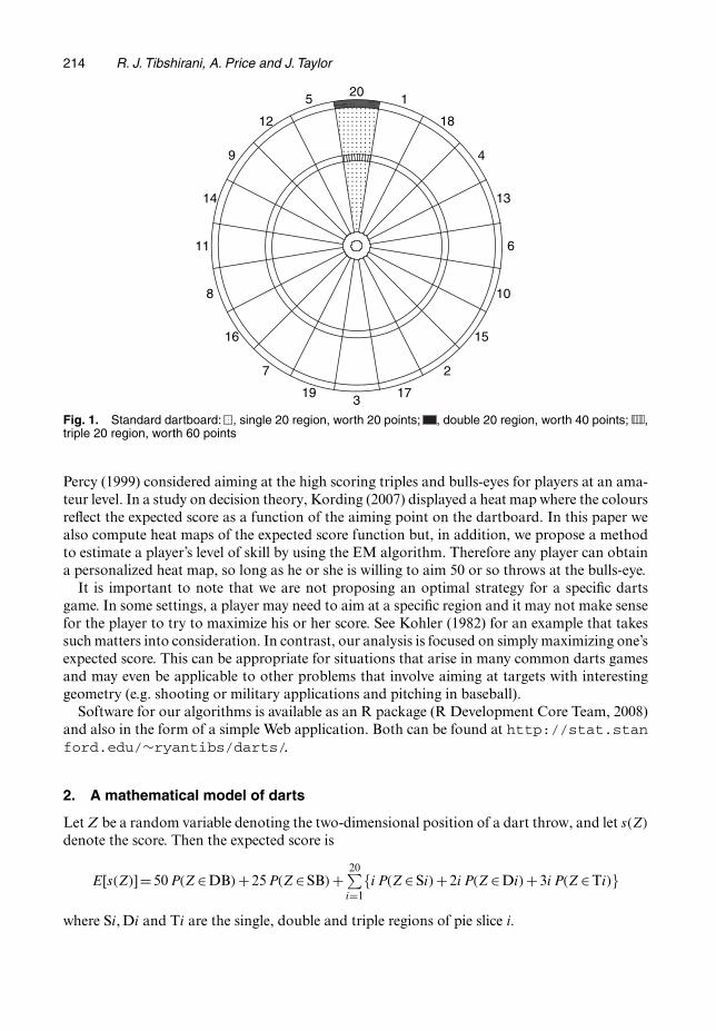
Familiar to most, the game of darts is played by throwing small metal missiles (darts) at a cir-cular target (dartboard). Fig. 1 shows a standard dartboard. A player receives a different scorefor landing a dart in different sections of the board. In most common dart games, the board’ssmall concentric circle, called the ‘double bulls-eye’ (DB) or just ‘bulls-eye’, is worth 50 points.The surrounding ring, called the ‘single bulls-eye’ (SB), is worth 25. The rest of the board isdivided into 20 pie-sliced sections, each having a different point value from 1 to 20. There is a‘doubles’ ring and a ‘triples’ ring spanning these pie slices, which multiply the score by a factorof 2 or 3 respectively.

Not being expert dart players, but statisticians, we were curious whether there is some way tooptimize our score. In Section 2, under a simple Gaussian model for dart throws, we describean efficient method to try to optimize your score by choosing an optimal location at which toaim. If you can throw relatively accurately (as measured by the variance in a Gaussian model),there are some surprising places that you might consider aiming the dart.

The optimal aiming spot changes depending on the variance. Hence we describe an algorithmby which you can estimate your variance based on the scores of as few as 50 throws aimed at theDB. The algorithm is a straightforward implementation of the EM algorithm (Dempster et al.,1977), and the simple model that we consider allows a closed form solution. In Sections 3 and 4we consider more realistic models, Gaussian with general covariance and skew Gaussian, andwe turn to importance sampling (Liu, 2008) to approximate the expectations in the E-steps. TheM-steps, however, remain analogous to the maximum likelihood calculations; therefore we feelthat these provide nice teaching examples to introduce the EM algorithm in conjunction withMonte Carlo methods.

Not surprisingly, we are not the first to consider optimal scoring for darts: Stern (1997) com-pared aiming at the triple 19 and triple 20 for players with an advanced level of accuracy, and

Address for correspondence: Ryan J. Tibshirani, Department of Statistics, Stanford University, 390 Serra Mall,Stanford, CA 94306, USA.E-mail: ryantibs@stanford.edu

214 R. J. Tibshirani, A. Price and J. Taylor

201

18

4

13

6

10

15

2

17319

7

16

8

11

14

9

12

5

Fig. 1. Standard dartboard: , single 20 region, worth 20 points; , double 20 region, worth 40 points; ,triple 20 region, worth 60 points

Percy (1999) considered aiming at the high scoring triples and bulls-eyes for players at an ama-teur level. In a study on decision theory, Kording (2007) displayed a heat map where the coloursreflect the expected score as a function of the aiming point on the dartboard. In this paper wealso compute heat maps of the expected score function but, in addition, we propose a methodto estimate a player’s level of skill by using the EM algorithm. Therefore any player can obtaina personalized heat map, so long as he or she is willing to aim 50 or so throws at the bulls-eye.

It is important to note that we are not proposing an optimal strategy for a specific dartsgame. In some settings, a player may need to aim at a specific region and it may not make sensefor the player to try to maximize his or her score. See Kohler (1982) for an example that takessuch matters into consideration. In contrast, our analysis is focused on simply maximizing one’sexpected score. This can be appropriate for situations that arise in many common darts gamesand may even be applicable to other problems that involve aiming at targets with interestinggeometry (e.g. shooting or military applications and pitching in baseball).

Software for our algorithms is available as an R package (R Development Core Team, 2008)and also in the form of a simple Web application. Both can be found at http://stat.stanford.edu/∼ryantibs/darts/.

2. A mathematical model of darts

Let Z be a random variable denoting the two-dimensional position of a dart throw, and let s.Z/

denote the score. Then the expected score is

E[s.Z/]=50P.Z ∈DB/+25P.Z ∈SB/+20∑

i=1{iP.Z ∈Si/+2iP.Z ∈Di/+3iP.Z ∈Ti/}

where Si, Di and Ti are the single, double and triple regions of pie slice i.

Darts 215

Perhaps the simplest model is to suppose that Z is uniformly distributed on the board B, i.e.for any region S

P.Z ∈S/= area.S ∩B/

area.B/:

Using the board measurements given in Appendix A.1, we can compute the appropriate prob-abilities (areas) to obtain

E[s.Z/]= 370619:807528900

≈12:82:

Surprisingly, this is a higher average than is achieved by many beginning players. (The firstauthor scored an average of 11.65 over 100 throws, and he was trying his best!) How can thisbe? First, a beginner will occasionally miss the board entirely, which corresponds to a score of0. But, more importantly, most beginners aim at the 20 region; since this is adjacent to the 5and 1 regions, it may not be advantageous for a sufficiently inaccurate player to aim here.

A follow-up question is: where is the best place to aim? As the uniform model is not a veryrealistic model for dart throws, we turn to the Gaussian model as a natural extension. Later, inSection 3, we consider a Gaussian model with a general covariance matrix. Here we consider asimpler spherical model. Let the origin .0, 0/ correspond to the centre of the board, and considerthe model

Z =μ+ ", "∼N .0, σ2I/

where I is the 2×2 identity matrix. The point μ= .μx, μy/ represents the location at which theplayer is aiming, and σ2 controls the size of the error ". (Smaller σ2 means a more accurateplayer.) Given this set-up, our question becomes: what choice of μ produces the largest value ofEμ,σ2 [s.Z/]?

2.1. Choosing where to aimFor a given σ2, consider choosing μ to maximize

Eμ,σ2 [s.Z/]=∫∫

12πσ2 exp

{− ‖.x, y/−μ‖2

2σ2

}s.x, y/dx dy: .1/

Although this is too difficult to approach analytically, we note that this quantity is simply

.fσ2Ås/.μ/

where ‘Å’ represents a convolution, in this case, the convolution of the bivariate N .0, σ2I/ densityfσ2 with the score s. In fact, by the convolution theorem

fσ2Ås=F−1{F.fσ2/F.s/}where F and F−1 denote the Fourier transform and inverse Fourier transform respectively. Thuswe can make two two-dimensional arrays of the Gaussian density and the score function eval-uated, say, on a millimetre scale across the dartboard, and rapidly compute their convolutionby using two fast Fourier transforms and one inverse fast Fourier transform.

Once we have computed this convolution, we have the expected score (1) evaluated at everyμ on a fine grid. It is interesting to note that this simple convolution idea was not noted in theprevious work on statistical modelling of darts (Stern, 1997; Percy, 1999), with the authors usinginstead naive Monte Carlo methods to approximate the above expectations. This convolution

216 R. J. Tibshirani, A. Price and J. Taylor

approach is especially useful for creating a heat map of the expected score, which would beinfeasible to compute using Monte Carlo methods.

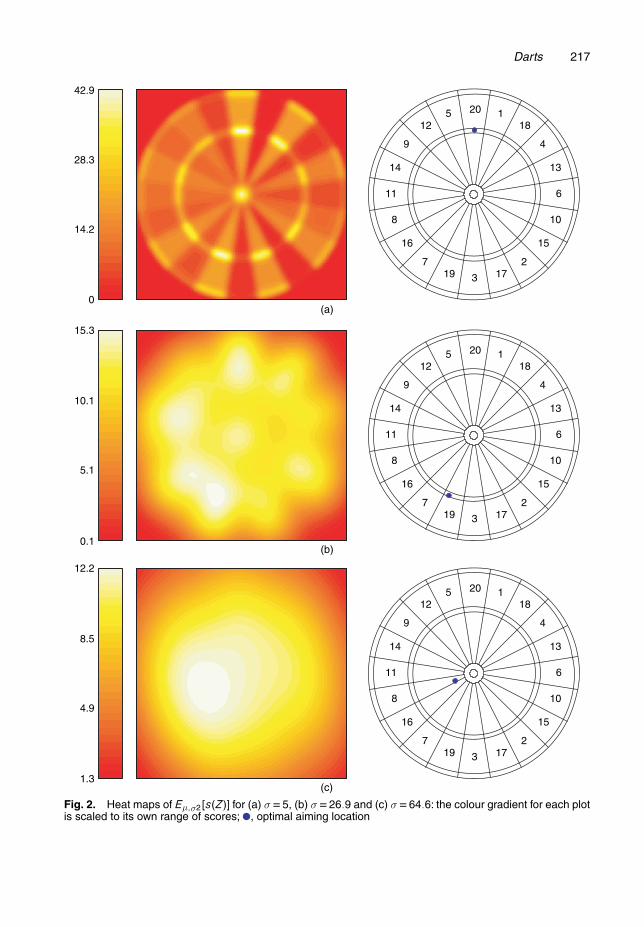
Some heat maps are shown in Fig. 2, for σ = 5, 26:9, 64:6. The last two values were chosenbecause, as we shall see shortly, these are estimates of σ that correspond to author 2 and author1 respectively. Here σ is given in millimetres; for reference, the board has a radius of 170 mm,and recall the rest of the measurements in Appendix A.1.

The bright colours (from yellow to white) correspond to the high expected scores. It is impor-tant to note that the heat maps change considerably as we vary σ. For σ =0 (perfect accuracy),the optimal μ lies in the triple 20 area, which is the highest scoring region of the board. Whenσ = 5, the best place to aim is still (the centre of) the triple 20 area. But, for σ = 26:9, it turnsout that the best place to aim is in the triple 19 region, close to the border that it shares with the7. For σ =64:6, one can achieve essentially the same (maximum) expected score by aiming in alarge spot around the centre, and the optimal spot is to the lower left of the bulls-eye.

2.2. Estimating the accuracy of a playerSince the optimal location μÅ.σ/ depends strongly on σ, we consider a method for estimating aplayer’s σ2 so that he or she can implement the optimal strategy. Suppose that a player throws nindependent darts, aiming each time at the centre of the board. If we knew the board positionsZ1, . . . , Zn, the standard sample variance calculation would provide an estimate of σ2. However,having a player record the position of each throw would be too time consuming and prone tomeasurement error. Also, few players would want to do this for a large number of throws; it ismuch easier instead just to record the score of each dart throw.

In what follows, we use just the scores to arrive at an estimate of σ2. This may seem surprisingat first, because there seems relatively little information to estimate σ2 just knowing the score,which for most numbers (e.g. 13) restricts the position to lie in a relatively large region (pie slice)of the board. This ambiguity is resolved by scores uniquely corresponding to the bulls-eyes,double rings and triple rings, and so it is helpful to record many scores. Unlike recording thepositions, it seems a reasonable task to record at least n=50 scores.

Since we observe incomplete data, this problem is well suited to an application of the EMalgorithm (Dempster et al., 1977). This algorithm, which is used widely in applied statistics, wasintroduced for problems in which maximization of a likelihood based on complete (but unob-served) data Z is simple, and the distribution of the unobserved Z based on the observationsX is somewhat tractable or at least easy to simulate from. In our setting, the observed data arethe scores X= .X1, . . . , Xn/ for a player aiming n darts at the centre μ=0, and the unobserveddata are the positions Z = .Z1, . . . , Zn/ where the darts actually landed.

Let l.σ2; X, Z/ denote the complete-data log-likelihood. The EM algorithm (in this case esti-mating only one parameter, σ2) begins with an initial estimate σ2

0, and then repeats the followingtwo steps until convergence:

(a) E-step—compute Q.σ2/=Eσ2t[l.σ2; X, Z/|X];

(b) M-step—let σ2t+1 =arg maxσ2{Q.σ2/}.

With μ=0, the complete-data log-likelihood is (up to a constant)

l.σ2; X, Z/={

−n log.σ2/− .1=2σ2/Σni=1 .Z2

i,x +Z2i,y/ if Xi = s.Zi/ ∀i,

−∞ otherwise.

Therefore the expectation in the E-step is

Eσ20[l.σ2; X, Z/|X]=−n log.σ2/− 1

2σ2

n∑i=1

Eσ20[Z2

i,x +Z2i,y|Xi]:

Darts 217

20 118

4

13

6

10

15

217319

7

16

8

11

14

9

125

20 118

4

13

6

10

15

217319

7

16

8

11

14

9

125

20 118

4

13

6

10

15

217319

7

16

8

11

14

9

125

42.9

0

14.2

28.3

15.3

0.1

5.1

10.1

12.2

1.3

4.9

8.5

(a)

(b)

(c)

Fig. 2. Heat maps of Eμ;σ2 [s.Z/] for (a) σ D5, (b) σ D26:9 and (c) σ D64:6: the colour gradient for each plotis scaled to its own range of scores; , optimal aiming location

218 R. J. Tibshirani, A. Price and J. Taylor

020

4060

8010

0

0 20 40 60 80 100True σ

Est

imat

ed σ

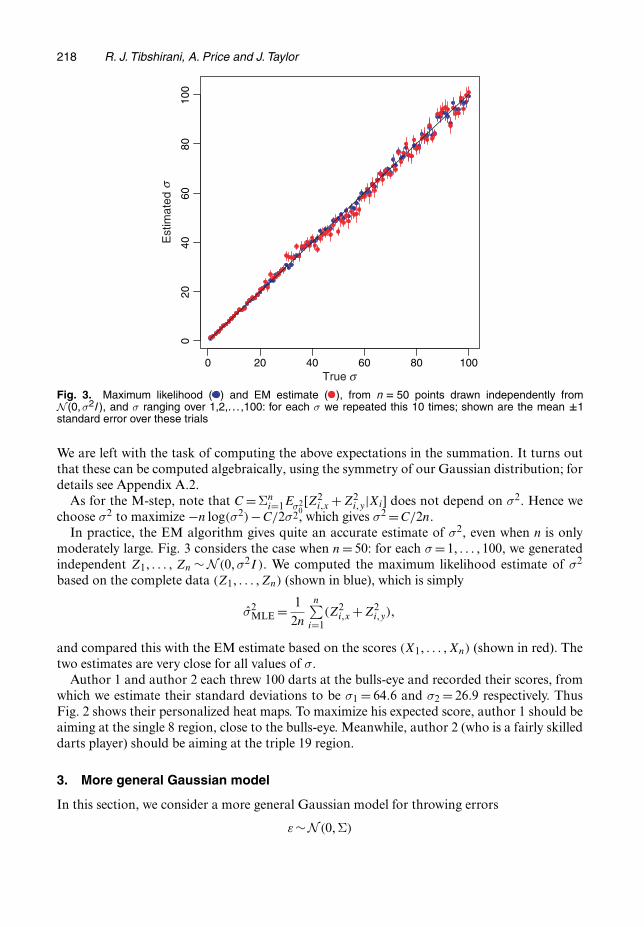
Fig. 3. Maximum likelihood ( ) and EM estimate ( ), from n D 50 points drawn independently fromN .0,σ2I /, and σ ranging over 1,2,. . . ,100: for each σ we repeated this 10 times; shown are the mean ˙1standard error over these trials

We are left with the task of computing the above expectations in the summation. It turns outthat these can be computed algebraically, using the symmetry of our Gaussian distribution; fordetails see Appendix A.2.

As for the M-step, note that C =Σni=1Eσ2

0[Z2

i,x + Z2i,y|Xi] does not depend on σ2. Hence we

choose σ2 to maximize −n log.σ2/−C=2σ2, which gives σ2 =C=2n.In practice, the EM algorithm gives quite an accurate estimate of σ2, even when n is only

moderately large. Fig. 3 considers the case when n= 50: for each σ = 1, . . . , 100, we generatedindependent Z1, . . . , Zn ∼ N .0, σ2I /. We computed the maximum likelihood estimate of σ2

based on the complete data .Z1, . . . , Zn/ (shown in blue), which is simply

σ̂2MLE = 1

2n

n∑i=1

.Z2i,x +Z2

i,y/,

and compared this with the EM estimate based on the scores .X1, . . . , Xn/ (shown in red). Thetwo estimates are very close for all values of σ.

Author 1 and author 2 each threw 100 darts at the bulls-eye and recorded their scores, fromwhich we estimate their standard deviations to be σ1 = 64:6 and σ2 = 26:9 respectively. ThusFig. 2 shows their personalized heat maps. To maximize his expected score, author 1 should beaiming at the single 8 region, close to the bulls-eye. Meanwhile, author 2 (who is a fairly skilleddarts player) should be aiming at the triple 19 region.

3. More general Gaussian model

In this section, we consider a more general Gaussian model for throwing errors

"∼N .0, Σ/

Darts 219

which allows for an arbitrary covariance matrix Σ. This flexibility is important, as a player’sdistribution of throwing errors may not be circularly symmetric. For example, it is common formost players to have a smaller variance in the horizontal direction than in the vertical direc-tion, since the throwing motion is up and down with no (intentional) lateral component. Also, aright-handed player may have a different ‘tilt’ to his or her error distribution (defined by the signof the correlation) than a left-handed player. In this new setting, we follow the same approachas before: first we estimate model parameters by using the EM algorithm; then we compute aheat map of the expected score function.

3.1. Estimating the covarianceWe can estimate Σ by using a similar EM strategy to that before, having observed the scoresX1, . . . , Xn of throws aimed at the board’s centre, but not the positions Z1, . . . , Zn. As μ=0, thecomplete-data log-likelihood is

l.Σ; X, Z/=−n

2log |Σ|− 1

2

n∑i=1

ZTi Σ−1Zi

with Xi = s.Zi/ for all i. It is convenient to simplify

n∑i=1

ZTi Σ−1Zi = tr

(Σ−1

n∑i=1

ZiZTi

)

using the fact that the trace is linear and invariant under commutation. Thus we must compute

EΣ0 [l.Σ; X, Z/|X]=−n

2log |Σ|− 1

2tr(

Σ−1n∑

i=1EΣ0 [ZiZ

Ti |Xi]

):

Maximization over Σ is a problem which is identical to that of maximum likelihood for a multi-variate Gaussian distribution with unknown covariance. Hence the usual maximum likelihoodcalculations (see Mardia et al. (1979)) give

Σ= 1n

n∑i=1

EΣ0 [ZiZTi |Xi]:

The expectations above can no longer be done in closed form as in the simple Gaussiancase. Hence we use importance sampling (Liu, 2008), which is a popular and useful MonteCarlo technique to approximate expectations that may be otherwise difficult to compute. Forexample, consider the term

EΣ0 [Z2i,x|Xi] =

∫∫x2p.x, y/dxdy,

where p is the density of Zi|Xi (Gaussian conditional on being in the region of the board definedby the score Xi). In practice, it is difficult to draw samples from this distribution, and hence it isdifficult to estimate the expectation by simple Monte Carlo simulation. The idea of importancesampling is to replace samples from p with samples from some q that is ‘close’ to p but easier todraw from. As long as p=0 whenever q=0, we can write∫∫

x2 p.x, y/dxdy =∫∫

x2 w.x, y/q.x, y/dxdy

where w =p=q. Drawing samples z1, . . . , zm from q, we estimate this quantity by

220 R. J. Tibshirani, A. Price and J. Taylor

1m

m∑j=1

z2i,x w.zi,x, zi,y/

or, if the density is known only up to some constant,

1m

m∑j=1

z2i,x w.zi,x, zi,y/

/1m

m∑j=1

w.zi,x, zi,y/:

There are many choices for q, and the optimal q, measured in terms of the variance of theestimate, is proportional to x2 p.x, y/ (Liu, 2008). In our case, we choose q to be the uniformdistribution over the region of the board that is defined by the score Xi, because these distribu-tions are easy to draw from. The weights in this case are easily seen to be just w.x, y/=fΣ0.x, y/,which is the bivariate Gaussian density with covariance Σ0.

3.2. Computing the heat mapHaving estimated a player’s covariance Σ, a personalized heat map can be constructed just asbefore. The expected score if the player tries to aim at a location μ is

.fΣÅs/.μ/:

Again we approximate this by evaluating fΣ and s over a grid and taking the convolution ofthese two two-dimensional arrays, which can be quickly computed by using two fast Fouriertransforms and one inverse fast Fourier transform.

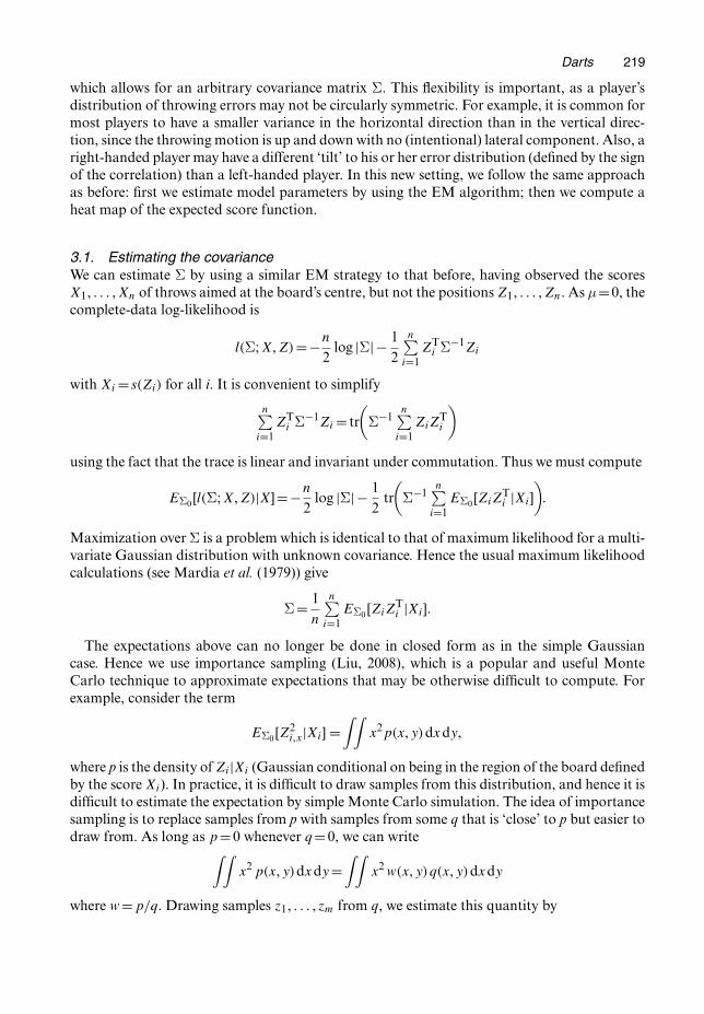
From their same set of n = 100 scores (as before), we estimate the covariances for author 1and author 2 to be

Σ1 =(

1820:6 −471:1−471:1 4702:2

),

Σ2 =(

320:5 −154:2−154:2 1530:9

)

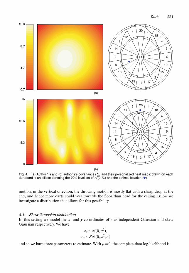
respectively. See Fig. 4 for their personalized heat maps.The flexibility in this new model leads to some interesting results. For example, consider

the case of author 2: from the scores of his 100 throws aimed at the bulls-eye, recall that weestimate his marginal standard deviation to be σ=26:9 according to the simple Gaussian model.The corresponding heat map instructs him to aim at the triple 19 region. However, under themore general Gaussian model, we estimate his x and y standard deviations to be σx =17:9 andσy =39:1, and the new heat map tells him to aim slightly above the triple 20 region. This changeoccurs because the general model can adapt to the fact that author 2 has substantially betteraccuracy in the x-direction. Intuitively, he should be aiming at the 20 area since his darts willoften remain in this (vertical) pie slice, and he will not hit the 5 or 1 areas (horizontal errors)sufficiently often for it to be worthwhile aiming elsewhere.

4. Model extensions and considerations

The Gaussian distribution is a natural model in the EM context because of its simplicity and itsubiquity in statistics. Additionally, there are many studies from cognitive science indicating that,in motor control, movement errors are indeed Gaussian (see Trommershauser et al. (2005), forexample). In the context of dart throwing, however, it may be that the errors in the y-directionare skewed downwards. An argument for this comes from an analysis of a player’s dart throwing

Darts 221

20 118

4

13

6

10

15

217319

7

16

8

11

14

9

125

(a)

(b)

201

18

4

13

6

10

15

217319

7

16

8

11

14

912

5

12.8

0.7

4.7

8.7

16

0

5.3

10.6

Fig. 4. (a) Author 1’s and (b) author 2’s covariances Σi and their personalized heat maps: drawn on eachdartboard is an ellipse denoting the 70% level set of N .0,Σi / and the optimal location ( )

motion: in the vertical direction, the throwing motion is mostly flat with a sharp drop at theend, and hence more darts could veer towards the floor than head for the ceiling. Below weinvestigate a distribution that allows for this possibility.

4.1. Skew Gaussian distributionIn this setting we model the x- and y-co-ordinates of " as independent Gaussian and skewGaussian respectively. We have

"x ∼N .0, σ2/,

"y ∼SN .0, ω2, α/

and so we have three parameters to estimate. With μ=0, the complete-data log-likelihood is

222 R. J. Tibshirani, A. Price and J. Taylor

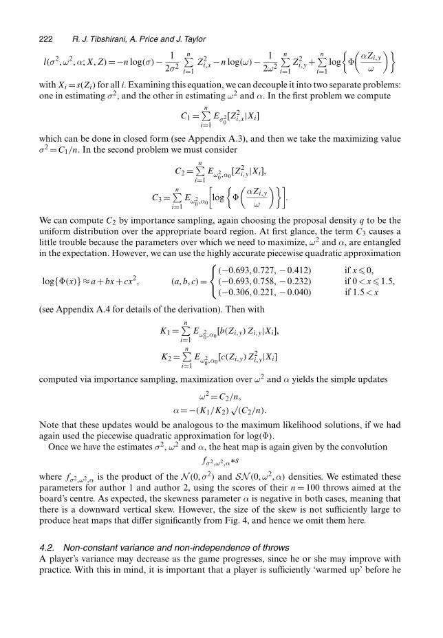
l.σ2, ω2, α; X, Z/=−n log.σ/− 12σ2

n∑i=1

Z2i,x −n log.ω/− 1

2ω2

n∑i=1

Z2i,y +

n∑i=1

log{

Φ(

αZi,y

ω

)}

with Xi = s.Zi/ for all i. Examining this equation, we can decouple it into two separate problems:one in estimating σ2, and the other in estimating ω2 and α. In the first problem we compute

C1 =n∑

i=1Eσ2

0[Z2

i,x|Xi]

which can be done in closed form (see Appendix A.3), and then we take the maximizing valueσ2 =C1=n. In the second problem we must consider

C2 =n∑

i=1Eω2

0 ,α0[Z2

i,y|Xi],

C3 =n∑

i=1Eω2

0 ,α0

[log

{Φ

(αZi,y

ω

)}]:

We can compute C2 by importance sampling, again choosing the proposal density q to be theuniform distribution over the appropriate board region. At first glance, the term C3 causes alittle trouble because the parameters over which we need to maximize, ω2 and α, are entangledin the expectation. However, we can use the highly accurate piecewise quadratic approximation

log{Φ.x/}≈a+bx+ cx2, .a, b, c/={

.−0:693, 0:727, −0:412/ if x�0,

.−0:693, 0:758, −0:232/ if 0 <x�1:5,

.−0:306, 0:221, −0:040/ if 1:5 <x

(see Appendix A.4 for details of the derivation). Then with

K1 =n∑

i=1Eω2

0 ,α0[b.Zi,y/Zi,y|Xi],

K2 =n∑

i=1Eω2

0 ,α0[c.Zi,y/Z2

i,y|Xi]

computed via importance sampling, maximization over ω2 and α yields the simple updates

ω2 =C2=n,

α=−.K1=K2/√

.C2=n/:

Note that these updates would be analogous to the maximum likelihood solutions, if we hadagain used the piecewise quadratic approximation for log.Φ/.

Once we have the estimates σ2, ω2 and α, the heat map is again given by the convolutionfσ2,ω2,αÅs

where fσ2,ω2,α is the product of the N .0, σ2/ and SN .0, ω2, α/ densities. We estimated theseparameters for author 1 and author 2, using the scores of their n = 100 throws aimed at theboard’s centre. As expected, the skewness parameter α is negative in both cases, meaning thatthere is a downward vertical skew. However, the size of the skew is not sufficiently large toproduce heat maps that differ significantly from Fig. 4, and hence we omit them here.

4.2. Non-constant variance and non-independence of throwsA player’s variance may decrease as the game progresses, since he or she may improve withpractice. With this in mind, it is important that a player is sufficiently ‘warmed up’ before he

Darts 223

20 1

18

4

13

6

10

15

2

17319

7

16

8

11

14

9

12

5

σ = 16.4

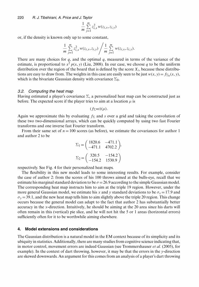
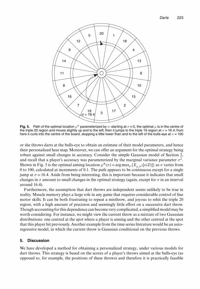
Fig. 5. Path of the optimal location μÅ parameterized by σ: starting at σ D0, the optimal μ is in the centre ofthe triple 20 region and moves slightly up and to the left; then it jumps to the triple 19 region at σ D16:4; fromhere it curls into the centre of the board, stopping a little lower than and to the left of the bulls-eye at σ D100

or she throws darts at the bulls-eye to obtain an estimate of their model parameters, and hencetheir personalized heat map. Moreover, we can offer an argument for the optimal strategy beingrobust against small changes in accuracy. Consider the simple Gaussian model of Section 2,and recall that a player’s accuracy was parameterized by the marginal variance parameter σ2.Shown in Fig. 5 is the optimal aiming location μÅ.σ/=arg maxμ{Eμ,σ2 [s.Z/]} as σ varies from0 to 100, calculated at increments of 0.1. The path appears to be continuous except for a singlejump at σ =16:4. Aside from being interesting, this is important because it indicates that smallchanges in σ amount to small changes in the optimal strategy (again, except for σ in an intervalaround 16.4).

Furthermore, the assumption that dart throws are independent seems unlikely to be true inreality. Muscle memory plays a large role in any game that requires considerable control of finemotor skills. It can be both frustrating to repeat a misthrow, and joyous to rehit the triple 20region, with a high amount of precision and seemingly little effort on a successive dart throw.Though accounting for this dependence can become very complicated, a simplified model may beworth considering. For instance, we might view the current throw as a mixture of two Gaussiandistributions: one centred at the spot where a player is aiming and the other centred at the spotthat this player hit previously. Another example from the time series literature would be an auto-regressive model, in which the current throw is Gaussian conditional on the previous throws.

5. Discussion

We have developed a method for obtaining a personalized strategy, under various models fordart throws. This strategy is based on the scores of a player’s throws aimed at the bulls-eye (asopposed to, for example, the positions of these throws) and therefore it is practically feasible

224 R. J. Tibshirani, A. Price and J. Taylor

for a player to gather the data needed. Finally, the strategy is represented by a heat map of theexpected score as a function of the aiming point.

Recall the simple Gaussian model that was presented in Section 2: here we were mainlyconcerned with the optimal aiming location. Consider the optimal (expected) score itself: notsurprisingly, the optimal score decreases as the variance σ2 increases. In fact, this optimalscore curve is very steep, and it nearly achieves exponential decline. We might ask whethermuch thought was put into the design of the current dartboard’s arrangement of the numbers1, . . . , 20. In researching this question, we found that the person who is credited with devis-ing this arrangement is Brian Gamlin, a carpenter from Bury, Lancashire, in 1896 (Chaplin,2009). Gamlin boasted that his arrangement penalized drunkards for their inaccuracy, but stillit remained unclear how he chose the particular sequence of numbers.

Therefore we decided to develop a quantitative measure for the difficulty of an arbitraryarrangement. Since every arrangement yields a different optimal score curve, we simply chosethe integral under this curve (over some finite limits) as our measure of difficulty. Hence a lowervalue corresponds to a more challenging arrangement, and we sought the arrangement thatminimized this criterion. Using the Metropolis–Hastings algorithm (Liu, 2008) we managed tofind an arrangement that achieves lower value of this integral than the current board; in fact,its optimal score curve lies below that of the current arrangement for every σ2.

Interestingly, the arrangement that we found is simply a mirror image of an arrangement thatwas given by Curtis (2004), which was proposed because it maximizes the sum of absolute differ-ences between adjacent numbers. Though this seems to be inspired by mathematical elegancemore than reality, it turned out to be unbeatable by our Metropolis–Hastings search! Supple-mentary materials (including a longer discussion of our search for challenging arrangements)are available at http://stat.stanford.edu/∼ryantibs/darts/.

Acknowledgements

We thank Rob Tibshirani for stimulating discussions and his great input. We also thank PatrickChaplin for his eager help concerning the history of the dartboard’s arrangement. Finally wethank the Joint Editor and referees, whose comments led to significant improvements in thispaper.

Appendix A

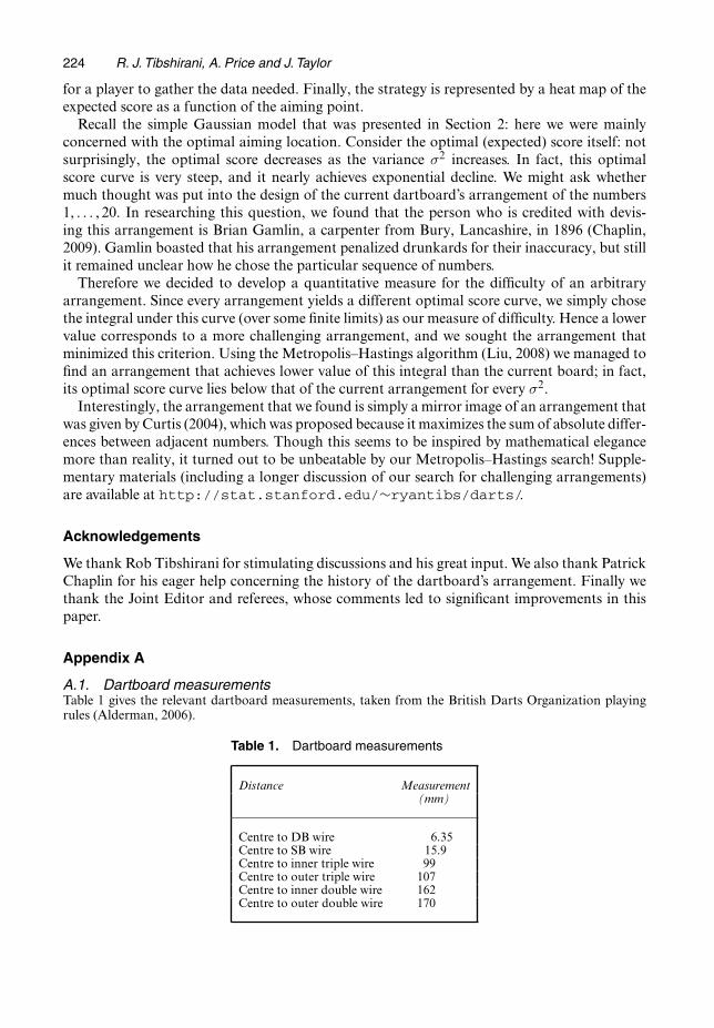
A.1. Dartboard measurementsTable 1 gives the relevant dartboard measurements, taken from the British Darts Organization playingrules (Alderman, 2006).

Table 1. Dartboard measurements

Distance Measurement(mm)

Centre to DB wire 6.35Centre to SB wire 15.9Centre to inner triple wire 99Centre to outer triple wire 107Centre to inner double wire 162Centre to outer double wire 170

Darts 225

A.2. Computing conditional expectations for the simple Gaussian EM algorithmRecall that we are in the setting Zi ∼N .0, σ2

0I/ and we are to compute the conditional expectation E[Z2i,x +

Z2i,y|Xi], where Xi denotes the score Xi = s.Zi/. In general, we can describe a score Xi as being achieved

by landing in ∪j Aj , where each region Aj can be expressed as [rj,1, rj,2]× [θj,1, θj,2] in polar co-ordinates.For example, the score Xi =20 can be achieved by landing in three such regions: the two single 20 chunksand the double 10 region. So

E[Z2i,x +Z2

i,y|Xi]=E[Z2i,x +Z2

i,y|Zi ∈∪jAj ]

=

∑j

∫ ∫Aj

.x2 +y2/ exp{−.x2 +y2/=2σ20}dx dy

∑j

∫ ∫Aj

exp{−.x2 +y2/=2σ20}dx dy

=

∑j

∫ rj, 2

rj, 1

∫ θj, 2

θj, 1

r3 exp.−r2=2σ20/ dθ dr

∑j

∫ rj, 2

rj, 1

∫ θj, 2

θj, 1

r exp.−r2=2σ20/ dθ dr

where we used a change of variables to polar co-ordinates in the last step. The integrals over θ will contributea common factor of

θj,2 −θj,1 ={

2π if Xi =25 or Xi =50,π=10 otherwise

to both the numerator and the denominator, and hence this will cancel. The integrals over r can becomputed exactly (by using integration by parts in the numerator), and therefore we are left with

E[Z2i,x +Z2

i,y|Xi]=

∑j

{.r2j,1 +2σ2

0/ exp.−rj,1=2σ20/− .r2

j,2 +2σ20/ exp.−rj,2=2σ2

0/}∑

j

{exp.−rj,1=2σ20/− exp.−rj,2=2σ2

0/} :

A.3. Computing conditional expectations for the skew Gaussian EM algorithmHere we have Zi,x ∼N .0, σ2

0/ (recall that it is the y-component Zi,y that is skewed), and we need to computethe conditional expectation E[Zi,x|Xi]. Following the same arguments as in Appendix A.2, we have

E[Z2i,x|Xi]=

∑j

∫ rj, 2

rj, 1

∫ θj, 2

θj, 1

r3 cos2.θ/ exp.−r2=2σ20/ dθ dr

∑j

∫ rj, 2

rj, 1

∫ θj, 2

θj, 1

r exp.−r2=2σ20/dθ dr

:

This is only slightly more complicated, since the integrals over θ no longer cancel. We compute∫ θj, 2

θj, 1

cos2.θ/ dθ =Δθj=2+{sin.2θj,2/− sin.2θj,1/}=4

where Δθj =θj,2 −θj,1, and the integrals over r are the same as before, giving

E[Z2i,x|Xi]=

∑j

{.r2j,1 +2σ2

0/ exp.−rj,1=2σ20/− .r2

j,2 +2σ20/ exp.−rj,2=2σ2

0/}{2Δθj + sin.2θj,2/− sin.2θj,1/}∑

j

{exp.−rj,1=2σ20/− exp.−rj,2=2σ2

0/}×4Δθj

:

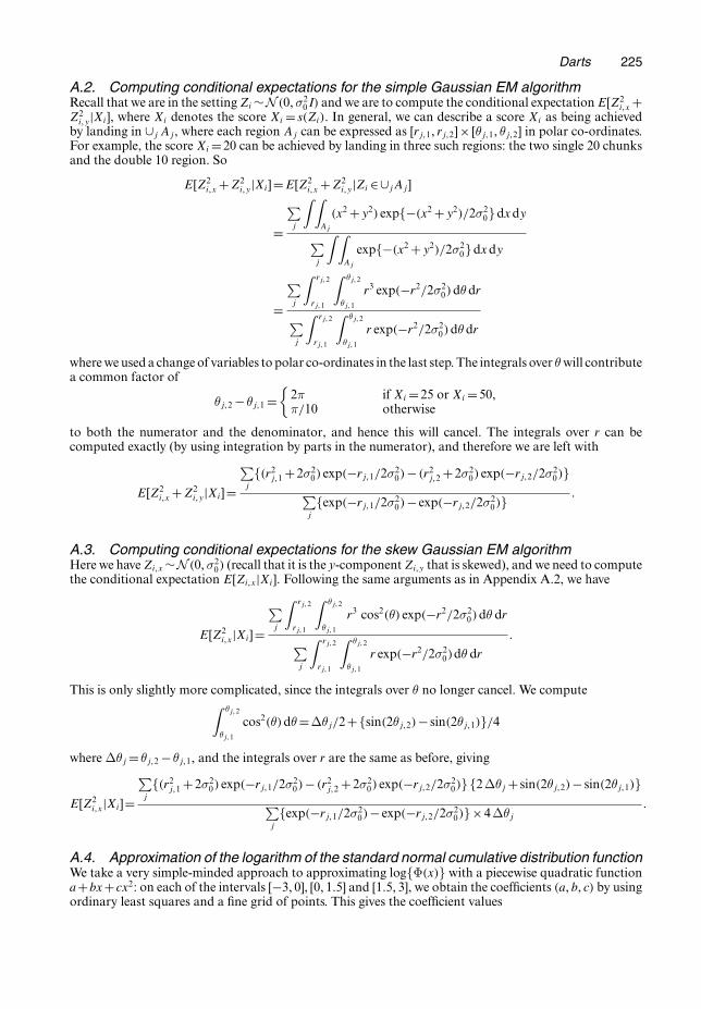
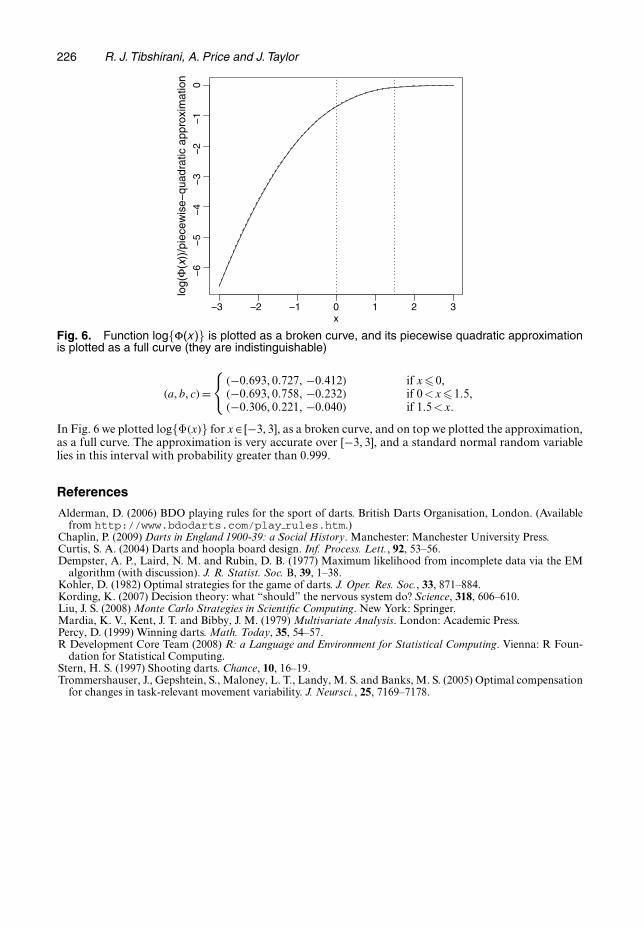
A.4. Approximation of the logarithm of the standard normal cumulative distribution functionWe take a very simple-minded approach to approximating log{Φ.x/} with a piecewise quadratic functiona+bx+cx2: on each of the intervals [−3, 0], [0, 1:5] and [1:5, 3], we obtain the coefficients .a, b, c/ by usingordinary least squares and a fine grid of points. This gives the coefficient values

226 R. J. Tibshirani, A. Price and J. Taylor

−3 −2 −1 0 1 2 3

−6

−5

−4

−3

−2

−1

0

x

log(

Φ(x

))/p

iece

wis

e−qu

adra

tic a

ppro

xim

atio

n

Fig. 6. Function log{F.x/} is plotted as a broken curve, and its piecewise quadratic approximationis plotted as a full curve (they are indistinguishable)

.a, b, c/={

.−0:693, 0:727, −0:412/ if x�0,

.−0:693, 0:758, −0:232/ if 0 <x�1:5,

.−0:306, 0:221, −0:040/ if 1:5 <x:

In Fig. 6 we plotted log{Φ.x/} for x∈ [−3, 3], as a broken curve, and on top we plotted the approximation,as a full curve. The approximation is very accurate over [−3, 3], and a standard normal random variablelies in this interval with probability greater than 0.999.

References

Alderman, D. (2006) BDO playing rules for the sport of darts. British Darts Organisation, London. (Availablefrom http://www.bdodarts.com/play rules.htm.)

Chaplin, P. (2009) Darts in England 1900-39: a Social History. Manchester: Manchester University Press.Curtis, S. A. (2004) Darts and hoopla board design. Inf. Process. Lett., 92, 53–56.Dempster, A. P., Laird, N. M. and Rubin, D. B. (1977) Maximum likelihood from incomplete data via the EM

algorithm (with discussion). J. R. Statist. Soc. B, 39, 1–38.Kohler, D. (1982) Optimal strategies for the game of darts. J. Oper. Res. Soc., 33, 871–884.Kording, K. (2007) Decision theory: what “should” the nervous system do? Science, 318, 606–610.Liu, J. S. (2008) Monte Carlo Strategies in Scientific Computing. New York: Springer.Mardia, K. V., Kent, J. T. and Bibby, J. M. (1979) Multivariate Analysis. London: Academic Press.Percy, D. (1999) Winning darts. Math. Today, 35, 54–57.R Development Core Team (2008) R: a Language and Environment for Statistical Computing. Vienna: R Foun-

dation for Statistical Computing.Stern, H. S. (1997) Shooting darts. Chance, 10, 16–19.Trommershauser, J., Gepshtein, S., Maloney, L. T., Landy, M. S. and Banks, M. S. (2005) Optimal compensation

for changes in task-relevant movement variability. J. Neursci., 25, 7169–7178.