A Statistical Approach to Modeling Wheel-Rail Contact Dynamics

A Statistical Approach to Modeling Wheel-Rail Contact

Dynamics

SayedMohammad Hosseini

Thesis submitted to the faculty of the

Virginia Polytechnic Institute and State University

in partial fulfillment of the requirements for the degree of

Master of Science

In

Mechanical Engineering

Mehdi Ahmadian, Chair

Robert B. Gramacy

Steve C. Southward

Reza Mirzaiefar

December 4, 2020

Blacksburg, Virginia

Keywords: Statistical modeling, wheel-rail contact, roller rig, experimental data,

longitudinal force, lateral force, creepage, angel of attack, wheel load, parametric

regression, support vector regression, distribution of predictions


Dynamics


(ABSTRACT)

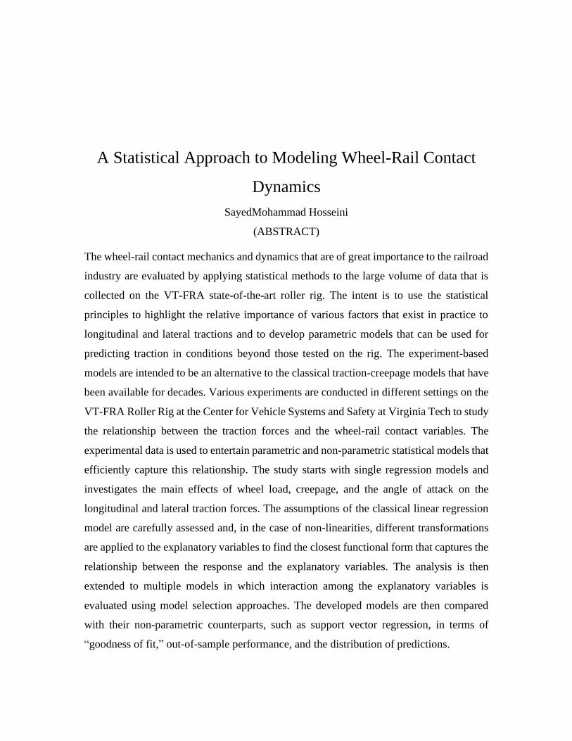
The wheel-rail contact mechanics and dynamics that are of great importance to the railroad

industry are evaluated by applying statistical methods to the large volume of data that is

collected on the VT-FRA state-of-the-art roller rig. The intent is to use the statistical

principles to highlight the relative importance of various factors that exist in practice to

longitudinal and lateral tractions and to develop parametric models that can be used for

predicting traction in conditions beyond those tested on the rig. The experiment-based

models are intended to be an alternative to the classical traction-creepage models that have

been available for decades. Various experiments are conducted in different settings on the

VT-FRA Roller Rig at the Center for Vehicle Systems and Safety at Virginia Tech to study

the relationship between the traction forces and the wheel-rail contact variables. The

experimental data is used to entertain parametric and non-parametric statistical models that

efficiently capture this relationship. The study starts with single regression models and

investigates the main effects of wheel load, creepage, and the angle of attack on the

longitudinal and lateral traction forces. The assumptions of the classical linear regression

model are carefully assessed and, in the case of non-linearities, different transformations

are applied to the explanatory variables to find the closest functional form that captures the

relationship between the response and the explanatory variables. The analysis is then

extended to multiple models in which interaction among the explanatory variables is

evaluated using model selection approaches. The developed models are then compared

with their non-parametric counterparts, such as support vector regression, in terms of

“goodness of fit,” out-of-sample performance, and the distribution of predictions.


Dynamics


(GENERAL AUDIENCE ABSTRACT)

The interaction between the wheel and rail plays an important role in the dynamic behavior

of railway vehicles. The wheel-rail contact has been extensively studied through analytical

models, and measuring the contact forces is among the most important outcomes of such

models. However, these models typically fall short when it comes to addressing the

practical problems at hand. With the development of a high-precision test rig—called the

VT-FRA Roller Rig, at the Center for Vehicle Systems and Safety (CVeSS)—there is an

increased opportunity to tackle the same problems from an entirely different perspective,

i.e. through statistical modeling of experimental data.

Various experiments are conducted in different settings that represent railroad operating

conditions on the VT-FRA Roller Rig, in order to study the relationship between wheel-

rail traction and the variables affecting such forces. The experimental data is used to

develop parametric and non-parametric statistical models that efficiently capture this

relationship. The study starts with single regression models and investigates the main

effects of wheel load, creepage, and the angle of attack on the longitudinal and lateral

traction forces. The analysis is then extended to multiple models, and the existence of

interactions among the explanatory variables is examined using model selection

approaches. The developed models are then compared with their non-parametric

counterparts, such as support vector regression, in terms of “goodness of fit,” out-of-sample

performance, and the distribution of the predictions.

The study develops regression models that are able to accurately explain the relationship

between traction forces, wheel load, creepage, and the angle of attack.

iv

Dedication

To GMCKS and my parents.

v

Acknowledgments

My sincere appreciation goes to my advisor Prof. Mehdi Ahmadian for his guidance,

encouragement, and patience. Without his dedicated support, the goal of this research project

would not have been realized.

I would like to thank other members of my committee for their time and advice, especially Dr.

Robert B. Gramacy whose insight and knowledge of the subject matter were illuminating

throughout the process.

Special thanks to my colleagues at CVeSS, especially my close friends Dr. Arash H. Ahangarnejad

and Dr. Ahmad Radmehr, for their kind support and their input to my work.

Last but not least, I am extremely grateful to GMCKS, and to my family for their unconditional

love and unceasing support throughout my life.

vi

Table of Contents

1 Introduction ........................................................................................................................ 1

1.1 Motivation .......................................................................................................1

1.2 Objectives ........................................................................................................2

1.3 Approach .........................................................................................................2

1.4 Contributions ...................................................................................................3

1.5 Outline .............................................................................................................4

2 Background ........................................................................................................................ 5

2.1 Wheel-rail Contact Mechanics, Contact Forces, and Influential Variables ....5

2.2 Test Rigs ..........................................................................................................7

2.2.1 Full-scale Rigs; the Course of Development ...........................................7

2.2.2 Scaled Rigs...............................................................................................8

2.3 Virginia Tech-Federal Railroad Administration Roller Rig .........................10

2.4 Predictive Models Based on Experimental Data Generated by Roller Rigs .11

3 Statistical Methods ........................................................................................................... 13

3.1 Linear Regression Model and Underlying Assumptions ..............................13

3.2 Best Subset Selection ....................................................................................15

3.3 Stepwise Model Selection Via BIC ...............................................................16

3.4 Least Absolute Shrinkage and Selection Operator (LASSO) .......................17

3.5 Principle Component Analysis ......................................................................17

3.6 Natural Cubic Splines....................................................................................18

3.7 Regression Trees and Random Forests .........................................................19

3.8 Support Vector Regression............................................................................20

3.9 Residual Bootstrap ........................................................................................22

3.10 Kolmogorov-Smirnov Test ...........................................................................22

3.10.1 Two-sample Kolmogorov–Smirnov Test ..............................................23

vii

4 Data Collection & Data Sets ............................................................................................ 25

5 Single Regression Models and Inference on the Main Effects of Explanatory Variables30

5.1 Regressing Longitudinal Force on Angle of Attack (AoA) ..........................30

5.1.1 Polynomial Regression Model ...............................................................30

5.1.2 Analysis of Residuals .............................................................................31

5.1.3 Non-parametric Models and Comparison ..............................................34

5.2 Regressing Lateral Force on Angle of Attack (AoA) ...................................36



5.2.3 Linear Model and Assumptions Check ..................................................39

5.2.4 Non-parametric Models and Comparison ..............................................40

5.3 Regressing Longitudinal Force on Creepage ................................................42



5.3.3 Comparison with Non-parametric Models.............................................46

5.3.4 Polynomial Regression Model Trained on Incremental Measurement ..48

5.4 Regressing Lateral Force on Creepage..........................................................50

5.4.1 Linear Regression Model and Assumptions Check ...............................50

5.5 Regressing Longitudinal Force on Wheel Load ............................................51


5.6 Regressing Lateral Force on Wheel Load .....................................................53


6 Multiple Regression Models ............................................................................................ 56

6.1 Multiple Regression Model for Lateral Force ...............................................57

6.1.1 Superposition of Main Effects ...............................................................57

6.1.2 Stepwise Model Selection via BIC ........................................................59

6.1.3 Best Subset Selection & LASSO ...........................................................61

6.1.4 Principal Component Analysis and the Importance of Variables ..........64

6.1.5 Selected Model.......................................................................................68

viii

6.2 Distribution of Predictions for Multiple Regression Model of Lateral Force71

6.3 Multiple Regression Model for Longitudinal Force .....................................76

6.3.1 Superposition of Main Effects and Importance of Variables .................76

6.3.2 Stepwise Model Selection via BIC ........................................................78

6.3.3 LASSO & Best Subset Selection ...........................................................80

6.3.4 Selected Model.......................................................................................81

6.4 Distribution of Predictions for Multiple Regression Model of Longitudinal Force

82

7 Conclusions and Recommendations ................................................................................ 88

7.1 Conclusions ...................................................................................................88

7.2 Recommendations for Future Studies ...........................................................90

Bibliography ............................................................................................................................ 92

ix

List of Figures

Figure 1: Wheelset and contact frames (excerpt from [7]) ............................................................. 5

Figure 2: VT-FRA Roller Rig with the adjustable degrees of freedom ........................................ 10

Figure 3: An example of normal Q–Q plots comparing independent standard normal data on the

Y-axis to a theoretical standard normal on the X-axis (excerpt from [54]) .................................. 15

Figure 4: Piecewise constant and linear functions fitted to some artificial data (excerpt from [55])

....................................................................................................................................................... 18

Figure 5: An example of a regression tree along with the partitions of two-dimensional feature

space and final decision tree (excerpt from [49]) ......................................................................... 20

Figure 6: Support vectors and corresponding weights in an SVR model (excerpt from [58]) ..... 21

Figure 7: Two-sample Kolmogorov–Smirnov statistic, where the red and blue lines are empirical

distribution functions, and the black arrow is the two-sample KS statistic (excerpt from [59]) .. 23

Figure 8: Longitudinal and lateral forces versus AoA at 2% creepage and the wheel load of 9600

N .................................................................................................................................................... 25

Figure 9: Continuous measurement of longitudinal and lateral forces at 0 degrees AoA and 9600

N wheel load while sweeping the creepage from 0 to 2% ............................................................ 26

Figure 10: Measured longitudinal force at various increments of creepage at 0 degrees AoA and

the wheel load of 9600 N .............................................................................................................. 27

Figure 11: Measurements of longitudinal and lateral forces at 0 degrees AoA and 2% creepage

while incrementally increasing the wheel load ............................................................................. 28

Figure 12: Measurements of longitudinal and lateral forces while changing AoA and creepage

continuously at various wheel load increments ............................................................................ 29

Figure 13: Regressing longitudinal force on AoA using a quadratic polynomial, (upper left panel)

longitudinal force versus AoA and the fitted regression line (upper right panel) studentized

residuals vs. fitted values (lower left panel), and normal Q-Q plot of residuals (lower right)

histogram of residuals ................................................................................................................... 32

x

Figure 14: Regressing longitudinal force on AoA using only the quadratic term ........................ 34

Figure 15: Natural cubic spline model for regressing longitudinal force on AoA, vertical lines show

the 1st, median, and the 3rd quantiles of AoA respectively ........................................................... 35

Figure 16: Out-of-sample performance of the models for regressing longitudinal force on AoA 35

Figure 17: Regression line and residual plots for regressing the lateral force on creepage using a

cubic polynomial ........................................................................................................................... 37

Figure 18: Transformations applied to AoA and lateral force to address heteroscedasticity ....... 38

Figure 19: Regression line and residual plots for regressing the lateral force on AoA ................ 40

Figure 20: Support vector regression model for regressing lateral force on AoA ........................ 41

Figure 21: Out-of-sample performance of the models for regressing lateral force on AoA......... 41

Figure 22: Regression line and residual plots for regressing the longitudinal force on creepage

using a quadratic polynomial ........................................................................................................ 43

Figure 23: Non-linear functions used to regress longitudinal force on creepage ......................... 44

Figure 24: Transformations applied to creepage and longitudinal force to fix heteroscedasticity 45

Figure 25: Natural cubic spline and residual plots for regressing longitudinal force on creepage47

Figure 26: Out-of-sample performance of the models for regressing longitudinal force on creepage

....................................................................................................................................................... 47

Figure 27: Regression line and the residuals plots for regressing the longitudinal force on creepage

using discrete measurement data .................................................................................................. 48

Figure 28: Regression line and residual plots for regressing the lateral force on creepage .......... 51

Figure 29: Regression line and residual plots for regressing the longitudinal force on wheel load

....................................................................................................................................................... 53

Figure 30: Regression line and residual plots for regressing the lateral force on wheel load ...... 54

Figure 31: Regression line and residual plots for regressing the lateral force on wheel load using a

smaller data set .............................................................................................................................. 55

Figure 32: Best subset selection criteria for choosing among the lateral force models ................ 62

Figure 33: Best subset selection criteria for choosing among the lateral force models (AoA linearly

varying with lateral force) ............................................................................................................. 63

xi

Figure 34: Percentage of variance explained by the main effects and their pairwise interactions,

excluding the AoA3 and its interactions across the principal components ................................... 65

Figure 35: Contribution of main effects and their pairwise interactions to the first principal

component (excluding AoA3 and its interactions) ........................................................................ 66

Figure 36: Contribution of main effects and their pairwise interactions to the second principal

component (excluding AoA3 and its interactions) ........................................................................ 66

Figure 37: Polar plot for the contribution of the main effects and their pairwise interactions to the

first and second principal component ........................................................................................... 67

Figure 38: Importance of variables in the random forest model of lateral force based on the average

decrease in node impurity ............................................................................................................. 68

Figure 39: Multiple regression model for lateral force, predictions and 95% confidence interval of

predictions ..................................................................................................................................... 72

Figure 40: SVR model for lateral force, predictions and 95% confidence interval of predictions73

Figure 41: Empirical CDF and density plot of the lower bounds of the 95% confidence interval of

predictions from the multiple regression model and the SVR model ........................................... 74

Figure 42: Empirical CDF and density plot of the upper bounds of the 95% confidence interval of

predictions from the multiple regression model and the SVR model ........................................... 75

Figure 43: Importance of variables in the random forest model of longitudinal force based on the

average decrease in node impurity ................................................................................................ 78

Figure 44: Best subset selection criteria for choosing among the longitudinal force models ...... 80

Figure 45: Multiple regression model for longitudinal force, predictions and 95% confidence

interval of predictions ................................................................................................................... 83

Figure 46: SVR model for longitudinal force, predictions and 95% confidence interval of

predictions ..................................................................................................................................... 84

Figure 47: CDF (upper panel) and density plot (lower panel) of the lower bounds of the 95%

confidence interval of predictions from the multiple regression model of longitudinal force and the

SVR model .................................................................................................................................... 85

xii

Figure 48: CDF (upper pane) and density plot (lower pane) of the upper bounds of the 95%

confidence interval of predictions from the multiple regression model of longitudinal force and the

SVR model .................................................................................................................................... 86

xiii

List of Tables

Table 1: VT-FRA Roller Rig measurement accuracy................................................................... 11

Table 2: Regression summary for regressing longitudinal force on AoA using a quadratic

polynomial .................................................................................................................................... 31

Table 3: Regression summary for regressing longitudinal force on AoA-squared ...................... 33

Table 4: Regression summary for regressing lateral force on AoA using a cubic polynomial .... 36

Table 5: Regression summary for regressing lateral force on AoA.............................................. 39

Table 6: Regression summary for regressing longitudinal force on creepage .............................. 42

Table 7: Regression summary for regressing longitudinal force on creepage using discrete data 49

Table 8: Regression summary for regressing lateral force on creepage ....................................... 50

Table 9: Regression summary for regressing longitudinal force on wheel load........................... 52

Table 10: Regression summary for regressing lateral force on wheel load .................................. 54

Table 11: Pairwise correlation of explanatory variables ............................................................... 56

Table 12: Regression summary for regressing lateral force on the main effects of explanatory

variables ........................................................................................................................................ 58

Table 13: Regression summary for regressing lateral force on the main effects of explanatory

variables (AoA linearly varying with lateral force) ...................................................................... 58

Table 14: Regression summary for the result of stepwise model selection via BIC for lateral force

....................................................................................................................................................... 59


(AoA linearly varying with lateral force) ..................................................................................... 60

Table 16: LASSO coefficient estimates for the lateral force model including AoA3 and its

interactions .................................................................................................................................... 63

Table 17: LASSO coefficient estimates for the lateral force model excluding AoA3 and its

interactions .................................................................................................................................... 64

xiv

Table 18: Adjusted R2 for the models incorporating the interaction of creepage and the wheel load

....................................................................................................................................................... 69

Table 19: Regression summary for the first alternative for modeling lateral force ...................... 69

Table 20: Regression summary for the second alternative for modeling lateral force ................. 70

Table 21: The Kolmogorov–Smirnov test for the lower bounds of the 95% confidence interval of

predictions from the multiple regression model of lateral force and the SVR model .................. 76

Table 22: The Kolmogorov–Smirnov test for the upper bounds of the 95% confidence interval of

predictions from the multiple regression model of lateral force and the SVR model .................. 76

Table 23: Regression summary for regressing longitudinal force on the main effects of explanatory

variables ........................................................................................................................................ 77

Table 24: Regression summary for the result of stepwise model selection via BIC for longitudinal

force .............................................................................................................................................. 79

Table 25: LASSO coefficient estimates for the longitudinal force model including all interactions

....................................................................................................................................................... 80

Table 26: Regression summary for the final model of longitudinal force .................................... 82


predictions from the multiple regression model of longitudinal force and the SVR model ......... 87


predictions from the multiple regression model of longitudinal force and the SVR model ......... 87

1

1 Introduction

1.1 Motivation

Data generated by test rigs under controlled conditions have been used for decades to study the

wheel-rail contact mechanics and dynamics and the factors affecting them. Traction and the factors

affecting it, as well as the influence of AoA and its role in derailment, have been extensively

studied by various researchers [1]–[6]. Most of these studies incorporate well-known contact

theories and use experimental data to validate established analytical models or to estimate the

parameters in such models.

The Virginia Tech-Federal Railroad Administration (VT-FRA) roller rig provides an excellent

opportunity for furthering some of the past studies because of its added precision in controlling

and measuring the factors that influence traction. The VT-FRA roller rig is also designed such that

it minimizes the contact patch distortion that is common to roller rigs. Through appropriate relative

sizing of the wheel to the roller, the contact patch distortion is kept to less than 10%. The same is

not true of many roller rigs that have been or are being used for traction studies in other research.

There is an immense opportunity to evaluate the fundamentals of wheel-rail contact mechanics

and dynamics from a more precise perspective. The VT-FRA Roller Rig is one of the most accurate

among the rigs currently in operation. It was designed and built for the specific goal of evaluating

the wheel-rail contact mechanics and dynamics with a high degree of precision. Its design allows

varying parameters such as % creepage, wheel load, cant angle, angle of attack, and lateral wheel-

rail position within a large range, hence allowing for evaluation of the extremes that could happen

in practice.

The high-precision data generated by the VT-FRA roller rig provides a great opportunity for

developing statistical models that would complement well-established analytical models. Such

models are being increasingly adopted by the industry due to the ever-increasing scope and

magnitude of field data that is gathered by the railroads and their suppliers. This study intends to

2

augment and improve the traction models that have been developed in the past through the

following objectives.

1.2 Objectives

This research aims to statistically model the dynamics of wheel and rail contact using the

experimental data generated by the VT-FRA Roller Rig. The objectives include:

1. Developing parametric and non-parametric single regression models for the traction

forces and the variables affecting them, including

a. The angle of attack (AoA)

b. Creepage, and

c. Wheel load;

2. Developing parametric and non-parametric multiple regression models for traction forces

by investigating the existence of interactions among the variables in addition to the

superposition of their main effects; and

3. Quantifying the uncertainty of predictions by the models through a comparison with

testing data.

1.3 Approach

The general approach to accomplishing the set goals is as follows:

1. Breaking the problem into two subproblems:

a. Predicting longitudinal forces

b. Predicting lateral forces

2. Studying the main effects of explanatory variables in isolation by single regression models

and using independent experiments:

a. Checking the assumptions of the classical linear regression model through the

analysis of residuals,

3

b. Applying transformations to capture any non-linearities, and

c. Comparison with non-parametric counterparts, e.g., natural splines, trees, and

random forests, and support vector regression in terms of:

i. In-sample performance

ii. Out-of-sample performance

3. Developing multiple regression models by combining the single models using model

selection methods such as stepwise model selection,

4. Developing non-parametric multiple regression models, and generating the distribution of

the prediction via empirical methods

5. Comparing parametric multiple regression models with the non-parametric models in terms

of distribution of predictions, including testing the equality of distributions using statistical

tests

1.4 Contributions

This research contributes to the advancement of railroad engineering both in theory and practice.

The major contributions of this research are:

• Addressing the wheel-rail contact modeling from an entirely new perspective, i.e.,

developing statistical models as opposed to the well-known analytical approaches,

• Providing a convenient means for predicting traction forces based on test data, without

requiring advanced algorithms and canned software

• Bridging the gap between the classical contact models and heuristic models that are based

on test data, and

• Creating an approach that allows adopting new machine/deep learning techniques for

predicting important effects, such as wheel and rail wear, based on controlled

measurements in the lab or field measurements from track inspection.

4

1.5 Outline

This document is organized as follows.

Chapter 2 reviews the contemporary literature in this field and introduces the specifications and

working principles of the VT-FRA Roller Rig. Chapter 3 gives a brief overview of the statistical

methods used for the analysis. The contents in this chapter progress logically starting from the

classical linear regression framework and evolving more advanced methods.

Chapter 4 deals with five data sets used in this research and the corresponding experiments, as well

as the testing conditions. Chapter 5 introduces the single regression models for the longitudinal

and lateral forces, along with an in-depth analysis of the residuals and the assumptions of the linear

regression model.

Chapter 6 summarizes the developed multiple regression models based on the single regression

models. This chapter is divided into two major sections: the multiple regression model of lateral

force, and the multiple regression model of longitudinal force. In either case, an ensemble of

various methods is used to provide compelling reasons for the conclusions drawn during the model

selection process. Finally, the confidence intervals of the predictions from the developed models

are compared with the empirical distribution of the predictions from the multiple support vector

regression models.

5

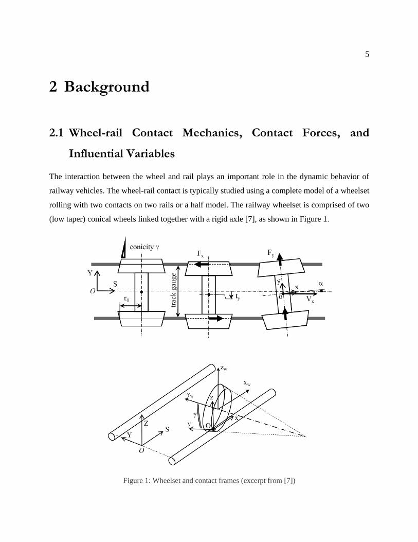
2 Background

2.1 Wheel-rail Contact Mechanics, Contact Forces, and

Influential Variables

The interaction between the wheel and rail plays an important role in the dynamic behavior of

railway vehicles. The wheel-rail contact is typically studied using a complete model of a wheelset

rolling with two contacts on two rails or a half model. The railway wheelset is comprised of two

(low taper) conical wheels linked together with a rigid axle [7], as shown in Figure 1.

Figure 1: Wheelset and contact frames (excerpt from [7])

6

Measuring the contact forces is among the most important outcomes of wheel-rail contact models,

and the angle of attack (AoA), creepage, and wheel load are considered to be the most important

variables that affect these forces. The theories that model the contact forces and address the

problem could be divided into two general categories:

• Normal contact models, either Hertzian or non-Hertzian

• Tangential contact models including, Kalker’s linear theory, FASTSIM, CONTACT, etc.

[8]

Each of these categories could also be subdivided into different classes. For instance, tangential

contact models are classified by Vollebregt [9] as:

• Fast and approximate approaches, e.g. FASTSIM2, Polach's method [10], and table-

lookup scheme

• Half-space-based approaches (physics-based theories), e.g. CONTACT [10], [11]

• Finite-element approaches

Various research studies have investigated the traction and traction forces at the wheel-rail contact.

Beak et al. [1] investigated the transient traction characteristics of two rollers' contact under dry

and lubricated conditions, and Spiryagin et al. [12] modeled creep force for rail traction vehicles

by modifying Kalker’s algorithm. Creep forces at the contact patch of the wheels and their

influence on the risk of railway vehicle derailments were also theoretically studied by Santamaria

et al. [13], while Jin et al. [14] studied how the elastic deformations of wheelset and track affect

the creep forces in rolling contact.

The influence of AoA and its role in derailment were investigated in [4]–[6]. The common attribute

of most of these studies is that they are either theoretical or use experimental data to quantify the

characteristics and parameters in standard theories and analytical models.

On the contrary, Alonso et al. [15] took an experimental approach towards characterizing the

wheel-rail contact problem and calculating contact forces by building a test-bench. This is an

example of various test rigs that were designed and built to perform repeatable tests.

7

2.2 Test Rigs

Various types of test rigs were developed to complement theoretical studies by generating

experimental data under various conditions as well as to improve railway vehicle performance in

a variety of applications [16]. The test rigs that simulate the wheel-rail contact fall into two major

categories:

1. Full-scale rigs that observe the actual sizes of the wheel and the rail(s)

2. Scaled rigs

In the following, well-known full-scale and scaled rigs and the objectives for their development

are enumerated.

2.2.1 Full-scale Rigs; the Course of Development

The two-axle roller rig at the Railway Technical Research Institute in Japan is one of the earliest

examples of full-scale rigs that was built in 1957 to simulate track irregularities, hunting,

derailment, etc. [7], [16], [17].

The German Federal Ministery of Research and Technology built a four-axle roller rig in 1977 to

study stability, ride comfort, and failure analysis [16]. The following year (1987), the

Transportation Technology Center, Inc. (TTCI) in the USA developed a four-axle roller rig to

study locomotive traction efforts, vehicle dynamics of passenger cars, and non-powered vehicles

[7]. The two-axle roller rig at the National Research Council in Canada was also developed in the

1980s to optimize bogie design and wear tests [18]–[20].

In 1992, a four-axle roller was built at the Ansaldo Transport Research Center in Naples, Italy to

investigate the traction effort of locomotives during transient states, and in 1995, the Sate Key

Laboratory of Traction Power in the Southwest Jiaotong University of China built a four-axle roller

rig for basic research on hunting stability, braking, traction, and derailment mechanisms [7]. The

latest full-scale rig was the single-wheel roller rig at the Voestalpine Schienen GmbH in Austria

that was built in 2000 to study rail wear, and rolling contact fatigue (RCF) [21].

8

2.2.2 Scaled Rigs

Scaled rigs followed the course of their development in parallel with their full-scale counterparts.

These rigs observe a ratio between the roller and the wheel. In the following, well-known scaled

rigs are chronologically enumerated.

• 1950s: The 1/5th- and 1/10th-scale rigs were developed at the Railway Research Institute in

Japan to improve the rail vehicle suspensions [14], [17], [22].

• 1980s:

o The single-axle 1/8th-scale roller rig was developed at the National Research

Council in Canada to study wheel-rail wear [16], [23].

o 1/4th-scale bogie on 13-m diameter rollers was developed at the Institut National de

Recherche sur les Transports et leur Securite to perform various tests, including

Kalker’s coefficients [24].

• 1984: The two-axle 1/5th-scale roller rig was developed on the dual disc-on-disc concept at

the German Oberpfaffenhofen to improve bogie and wheel designs, software models, and

limit cycle behaviors [25].

• 1992: The two-axle 1/5th-scale rig was developed at the Manchester Metropolitan

University to optimize suspension designs and study wheel-rail wear [26], [27].

• 1990s: The two-axle 2/7th-scale roller rig was developed at the Czech Technical University

in the Czech Republic to measure contact forces, and test active steering mechanisms [28]–

[30].

• 1995: The single-wheel roller at Sheffield University in England was developed to

experimentally study fatigue, wear, and third-body layer [31], [32].

• 2000s:

o The two-axle 1/5th-scale roller rig at Politecnico di Torino in Italy was developed

to study wheel-rail wear and dynamics of railcars [33]–[35].

o The single-axis 1/5th-roller rig at the National Traffic Safety & Environment

Laboratory in Japan was developed to study creep forces between the wheel and

roller [36].

9

o The two-axle 1/4th-scale roller rig at Jiaotong University in China was developed

to study wheel-rail wear, fatigue, and corrugation [37], [38].

• 2003: The two-axle 1/4th-scale roller rig at the Research Centre of Firenze Osmannoro in

Italy was developed to conduct hardware-in-the-loop operations and to test onboard safety

systems [39], [40].

• 2011: The two-axle 1/5th-scale roller rig at the Seoul National University of Science and

Technology in Korea was developed to study derailment [41], [42].

A careful review by Meymand et al. [43] showed that even though the experimental data generated

by these rigs resulted in major contributions to this field, there was still room for improvement,

both in terms of accuracy and versatility [16], [43]. With the advent of new technologies, a new

generation of high-precision scaled rigs were developed that could conduct a wider range of tests

in a consistent, repeatable manner [14]. The Virginia Tech-Federal Railroad Administration (VT-

FRA) Roller Rig is considered the next generation of high-precision rigs that became operational

in 2016. The capabilities and measurement accuracy of the VT-FRA Roller Rig are presented in

the following section.

10

2.3 Virginia Tech-Federal Railroad Administration Roller Rig

Figure 2: VT-FRA Roller Rig with the adjustable degrees of freedom

The Virginia Tech-Federal Railroad Administration (VT-FRA) Roller Rig is a novel system that

was designed and built with the specific goal of evaluating the wheel-rail contact mechanics and

dynamics with a high degree of precision. The rig consists of two rotating bodies in a vertical

configuration, a wheel that is 1/4th the scale of a 36-inch railcar, and a roller that is approximately

five times larger than a 44-inch locomotive wheel. The wheel and roller are driven by two

independent AC servo motors that can precisely control the rotating speed of each using motion

control techniques [16].

The rig is equipped with six linear electromagnetic actuators for accurately positioning the wheel

relative to the roller adjusting the simulated load. The rig is capable of actively controlling:

• Wheel load

Cant Angle

Lateral Displacement

Vertical Displacement

Angle of Attack

11

• The angle of attack (AoA)

• Lateral displacement

• Cant angle

The rig’s eight triaxial load cells can measure the three perpendicular components of quasi-static

forces in any direction and collect data while sweeping the range of other variables, such as the

Angle of Attack (AoA) and creepage [16]. The range of variables and their precision is such that

the rig can be used for a wide range of studies and repeated experiments indicated excellent

repeatability of results [44]. Table 1 shows the accuracy of measurements on the VT-FRA Roller

Rig.

Table 1: VT-FRA Roller Rig measurement accuracy

Scale 1:4

Angle of attack (deg.) ± 6 0.1 increments

Cant angle (deg.) ± 6 0.1 increments

Lateral displacement (inch) ± 1 4/1000 increments

Max. velocity (km/h/mph) 16 / 10 (scaled) 16 / 10 (full)

Max. Creep Rate (%) 10

Max. Contact Forces (per wheel-rail pair)

Normal Load (kN/KIPS) 12 / 2.7 (scaled) 192 / 43 (full)

Longitudinal Force (kN/KIPS) 16 / 3.6 (scaled) 256 / 57 (full)

Lateral Force (kN/KIPS) 16 / 3.6 (scaled) 57 (full)

2.4 Predictive Models Based on Experimental Data Generated

by Roller Rigs

The reach data generated by modern rigs have provided the opportunity to develop models that

could improve the economy, safety, and maintenance of railway vehicles by predicting important

variables using advanced statistical and AI methods. The use of machine learning techniques and

12

advanced predictive models, such as artificial neural networks, dates back to the 1980s and 1990s

and was primarily utilized for addressing scheduling problems [45], [46]. Parkinson and Iwnicki

[47] used these techniques to predict wheel and rail forces and to optimize railway suspension

systems [48] in the late 1990s and early 2000s. This trend has continued and become more

prevalent during the past few years. In 2018, Shebani and Iwnicki [45] developed an artificial

neural network to predict wheel-rail wear, and their research showed that the neural network can

be efficiently employed for this purpose. This new line of research takes an interdisciplinary

approach towards solving core engineering problems and aims at maximizing efficiency and

improving prediction accuracy by using advanced statistical/machine techniques.

13

3 Statistical Methods

This section gives an overview of the statistical method that will be used in the following chapters.

The main objective here is to lay the foundation for the statistical analysis carried out throughout

the study. We start with the classical linear regression model and the underlying assumptions. Then

we cover the selection methods, the best subset selection, and stepwise model selection in

particular. The principal component analysis is discussed next, followed by non-parametric models

e.g., natural splines, regression trees, and random forests, and support vector regression. The

chapter concludes with the residual bootstrap method and the Kolmogorov-Smirnov Test.

3.1 Linear Regression Model and Underlying Assumptions

Simple linear regression is a linear model for predicting a response 𝑌 from a single predictor

variable 𝑋 (or regressing 𝑌 on 𝑋), assuming that the relationship is approximately linear [49].

Mathematically,

𝑌 ≈ 𝛽0 + 𝛽1𝑋 + 𝜀

where 𝜀 is the random error (idiosyncratic noise) centered at zero. The coefficients are estimated

by minimizing the residual sum of squares

𝑅𝑆𝑆 = 𝑒12 + 𝑒2

2 + . . . + 𝑒𝑛2

𝑒𝑖 = 𝑦𝑖 − �̂�𝑖

where 𝑦𝑖 is the 𝑖𝑡ℎ value of response 𝑌, and �̂�𝑖 is the corresponding prediction based on the above

simple linear regression equation [49].

The coefficient of determination or R2 is defined as the proportion of variance explained by the

model. Mathematically,

𝑅2 = 𝑇𝑆𝑆 − 𝑅𝑆𝑆

𝑇𝑆𝑆= 1 −

𝑅𝑆𝑆

𝑇𝑆𝑆

14

where 𝑇𝑆𝑆 = ∑(𝑦𝑖 − �̅�𝑖)2 is called the total sum of squares [49], [50].

The simple regression model could be extended to more than one predictor. For 𝑝 distinct

predictors, the multiple linear regression model could be defined as follows:

𝑌 = 𝛽0 + 𝛽1𝑋1 + 𝛽2𝑋2+. . . + 𝛽𝑝𝑋𝑝 + 𝜀

𝑅𝑆𝑆 = ∑(𝑦𝑖 − �̂�𝑖)2

𝑛

𝑖=1

where 𝑦𝑖 is the 𝑖𝑡ℎ value of response 𝑌, and �̂�𝑖 is the corresponding prediction based on the multiple

regression equation and where the values of 𝛽𝑖’s that minimize it are the multiple least squares

regression coefficient estimates [49].

In order for the estimates of the multiple regression model and their variance to be valid, the

following assumptions must hold [51]:

1) Residuals are independent and identically distributed normals centered at zero with

constant variance, 𝜀𝑖~𝒩(0, 𝜎2) or more specifically:

o 𝔼[𝜀𝑖] = 0

o 𝕍𝑎𝑟(𝜀𝑖) = 𝔼[𝜀𝑖2] = 𝜎2

2) Regressors are uncorrelated with idiosyncratic noise (no endogeneity)

3) Regressors are identifiable, 𝕍𝑎𝑟(𝑋𝑖) > 0

The first assumption is of great importance since the predictions will be valid even if this

assumption does not hold (since the expectation, 𝔼[ ], is a linear operator), but the standard error

of the coefficient estimates (�̂�𝑖’s) and subsequently, the prediction intervals, will not be valid [51].

We will be using the scatter plot of studentized residuals versus fitted values to detect

heteroscedasticity or non-constant variance, and the normal Q-Q plot along with the histogram of

the residuals to check the normality assumption [52]. “The normal Q-Q plot is a graphical method

for comparing two probability distributions by plotting their quantiles against each other” [53]. It

compares the quantiles of a theoretical normal distribution with the quantiles of the sample.

15

Figure 3: An example of normal Q–Q plots comparing independent standard normal data on the Y-axis to

a theoretical standard normal on the X-axis (excerpt from [54])

It should be noted that a studentized version of the residuals will be used in analysis since the

population variance is estimated by sample variance, hence the residuals follow Student’s t-

distribution1. However, this is not necessary since t-distribution converges to a normal distribution

when the sample size is large enough.

3.2 Best Subset Selection

This approach selects a subset of the 𝑝 predictors that are believed to be highly related to the

response and solves the model of this subset using least squares. More specifically, the algorithm

fits a (least squares) regression to each possible combination2 (not limited to pairs of two) of the 𝑝

predictors and selects one based on the following criteria [49]:

• Cross-validated prediction error

1 t-distribution with k degrees of freedom is generated by dividing a normal by Chai-squared with k degrees of freedom

2 All the 2p subsets of a set of size p

16

• Cp (AIC3)

• BIC

• Adjusted R2 (R2 adjusted for the number of predictors)

Bayes Information Criterion or BIC is a criterion widely used for model selection and generally

discussed in information theory. Mathematically, BIC is defined as

𝐵𝐼𝐶 = −2 𝑙(�̂�, �̂�2) + 𝑝 𝑙𝑜𝑔 (𝑛)

where 𝑙 is the log-likelihood, (�̂�, �̂�2) is the Maximum Likelihood Estimator (MLE), 𝑝 is the

number of parameters, and 𝑛 is the number of observations [52].

An in-depth discussion of all the above criteria requires defining other statistical and mathematical

concepts and is beyond the scope of this thesis. Additional information is included in references

[49], [52], and [55].

3.3 Stepwise Model Selection Via BIC

Stepwise model selection is another approach toward selecting the best model describing the data.

“Forward stepwise selection starts with a model that contains no predictors and then adds more

predictors until the model contains all the predictors” [49]. At each step, the variable that improves

the fit to the greatest extent is added to the model [49]. More specifically, the greatest additional

improvement (while using BIC) translates into the model with the lowest BIC since the log-

likelihood is inherently negative. Using the BIC as the selection criterion balances the trade-off

between model complexity and lowest error [52]. Backward and forward-backward stepwise

model selection approaches follow the same procedure with minor differences in the direction of

building models.

3 Akaike Information Criterion

17

3.4 Least Absolute Shrinkage and Selection Operator

(LASSO)

The least absolute shrinkage and selection operator is a form of regularized regression. It takes the

“L1 norm” of the regression coefficient as the penalty function. Mathematically, it minimizes the

RSS plus a penalization term

�̂�𝜆𝐿𝐴𝑆𝑆𝑂 = 𝑎𝑟𝑔𝑚𝑖𝑛𝛽 ||𝑦 − 𝑋𝛽||2

2 + 𝜆 ∑ |𝛽𝑗|

𝑑

𝑗

This form of regularized regression is used for model selection purposes since the “L1 norm”

penalty function encourages sparse solutions resulting in automatic variable selection [49], [52].

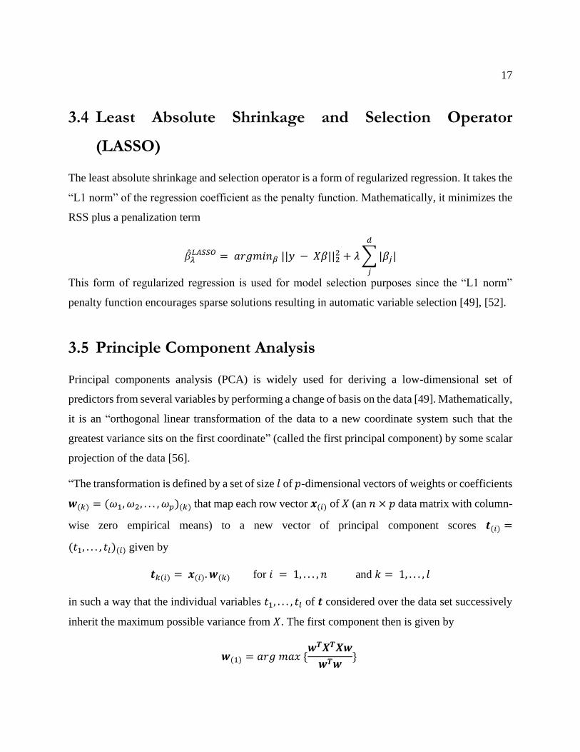
3.5 Principle Component Analysis

Principal components analysis (PCA) is widely used for deriving a low-dimensional set of

predictors from several variables by performing a change of basis on the data [49]. Mathematically,

it is an “orthogonal linear transformation of the data to a new coordinate system such that the

greatest variance sits on the first coordinate” (called the first principal component) by some scalar

projection of the data [56].

“The transformation is defined by a set of size 𝑙 of 𝑝-dimensional vectors of weights or coefficients

𝒘(𝑘) = (𝜔1, 𝜔2, . . . , 𝜔𝑝)(𝑘) that map each row vector 𝒙(𝑖) of 𝑋 (an 𝑛 × 𝑝 data matrix with column-

wise zero empirical means) to a new vector of principal component scores 𝒕(𝑖) =

(𝑡1, . . . , 𝑡𝑙)(𝑖) given by

𝒕𝑘(𝑖) = 𝒙(𝑖). 𝒘(𝑘) for 𝑖 = 1, . . . , 𝑛 and 𝑘 = 1, . . . , 𝑙

in such a way that the individual variables 𝑡1, . . . , 𝑡𝑙 of 𝒕 considered over the data set successively

inherit the maximum possible variance from 𝑋. The first component then is given by

𝒘(1) = 𝑎𝑟𝑔 𝑚𝑎𝑥 {𝒘𝑻𝑿𝑻𝑿𝒘

𝒘𝑻𝒘}

18

On this basis, the 𝑘𝑡ℎ-component can be found by subtracting the first 𝑘 − 1 principal components

from 𝑋:

�̂�𝑘 = 𝑋 − ∑ 𝑋𝒘(𝑠)𝒘(𝑘)𝑇

𝑘−1

𝑠=1

[57].”

The principal components are the eigenvectors of the covariance matrix. More specifically, the

principal axes are given by eigenvectors. and the variance along those axes are given by the square

of the corresponding eigenvalues [52].

3.6 Natural Cubic Splines

Piecewise splines are obtained by dividing the domain of 𝑋 into contiguous intervals and fitting

polynomials of different orders to each interval. Continuity and smoothness in piecewise splines

are attained by imposing restrictions on the first and second derivatives at knots [55].

Figure 4: Piecewise constant and linear functions fitted to some artificial data (excerpt from [55])

Generally speaking, splines suffer from erratic behavior in the first and last intervals. Natural cubic

splines fit piecewise linear functions to the first and last intervals, cubic polynomials to the rest,

and have continuous first and second derivatives at the knots. The degrees of freedom in natural

cubic splines equals the number of knots, and this leads to some nice mathematical properties for

19

their smoother matrices [55] which makes them one of the good choices for fitting regression lines

to the data with complex non-linear patterns.

This short introduction was provided to give an intuition about the concept; however, further

discussion of mathematical concepts, such as smoother matrices for natural cubic splines requires

defining other statistical and mathematical concepts that are beyond the scope of this thesis. For

more information, please refer to [49], [53].

3.7 Regression Trees and Random Forests

Regression Trees are presumably one of the simplest approaches to regression. They divide the

predictor space into non-overlapping regions (high-dimensional rectangles) by making a binary

split at each step that minimizes a criterion such as regression deviance and then fitting a simple

model (a constant) in each element of the partition [49], [52].

𝑅𝑒𝑔𝑟𝑒𝑠𝑠𝑖𝑜𝑛 𝐷𝑒𝑣𝑖𝑎𝑛𝑐𝑒 = ∑(𝑦𝑖 − �̂�𝑖)2

𝑛

𝑖=1

where �̂�𝑖 = �̅�𝑙𝑒𝑎𝑓 𝑡ℎ𝑎𝑡 𝑥𝑖 𝑏𝑒𝑙𝑜𝑛𝑔𝑠 𝑡𝑜

Predictions are made by returning the value of the fitted model or (the constant) for every

observation that falls into that region [49], [52]. An intuitive illustration of the process and the

outcome is shown in Figure 5.

Random forests are based on trees and are fitted to the data by bootstrapping or re-sampling with

replacement from both the rows and columns of feature matrix 𝑋 to learn a collection of trees.

Predictions depend on the leaf model and are made by taking the average prediction from fitted

trees:

𝐸[𝑌 | 𝑥] = 1

𝐵∑ 𝑇𝑏(𝑥)

𝐵

𝑏=1

where 𝑇𝑏 is the tree model and 𝐵 is the number of bootstrap samples (fitted trees) [49], [52].

20

Figure 5: An example of a regression tree along with the partitions of two-dimensional feature space and

final decision tree (excerpt from [49])

3.8 Support Vector Regression

Support vector regression employs the principles behind support vector machines to fit a regression

line to the data. Mathematically, this approach approximates the regression function in terms of a

set of basis functions, ℎ𝑚(𝑥), 𝑚 = 1, 2, … , 𝑀 [55]:

𝑓(𝑥) = ∑ 𝛽𝑚 ℎ𝑚(𝑥) + 𝛽0

𝑀

𝑚=1

21

This set of basis functions ℎ𝑚(𝑥) is transformed to a radial basis kernel, 𝑘(𝑥𝑖, 𝑥), and linear

coefficients or the Lagrange multipliers, (𝛼𝑖∗ − 𝛼𝑖), for each constraint in the feature space and

using the same optimization process used in support vector machines [58].

𝑓(𝑥) = ∑ (𝛼𝑖∗ − 𝛼𝑖) 𝑘(𝑥𝑖, 𝑥) + 𝛽0

𝑀

𝑖=1

Intuitively, this approach models the observations outside a specific margin around the regression

line (called support vector) with a univariate Gaussian centered at the observation and finds the

regression line by solving the constraint optimization problem to weigh the support vectors. Figure

6 shows this process figuratively.

Figure 6: Support vectors and corresponding weights in an SVR model (excerpt from [58])

The Lagrange multipliers define the importance of each Gaussian function.

Kernel places a Gaussian function on each support vector.

22

3.9 Residual Bootstrap

As opposed to the standard bagging approach or bootstrapping over the model, in this approach,

we bootstrap over the vector of residuals. We start with computing the residuals by subtracting the

predictions made by the regression model from the mean of the prediction or 𝑋�̂�, then we sample

from the residuals with replacement to construct a new 𝑌∗(𝑏) vector in each iteration by sampling

with replacement from the vector of residuals we have already computed. Mathematically, from

the regression model we have:

𝑌𝑖 = 𝑋𝑖�̂� + 𝜀𝑖

𝜀𝑖 = 𝑌𝑖 − 𝑋𝑖�̂�

Resampling with replacement from the vector of the residuals B times generates B bootstrap

samples via:

𝑌𝑖∗ = 𝑋𝑖�̂� + 𝜀𝑖

∗

(𝑋1∗(1), 𝑌1

∗(1)) . . . (𝑋𝑛∗(1), 𝑌𝑛

∗(1))

⋮ ⋮

(𝑋1∗(𝐵), 𝑌1

∗(𝐵)) . . . (𝑋𝑛∗(𝐵), 𝑌𝑛

∗(𝐵))

where 𝑋𝑖∗ = 𝑋𝑖 since 𝑋𝑖 did not change during resampling.

Having run the bootstrap loop for B iterations, we obtain B prediction vectors, 𝑌𝑖∗, using the design

matrix 𝑋 and the �̂� vector coming from the regression model fitted to the training set [55]. In the

end, we obtain a prediction vector of length B for each observation in the testing set, and using

these vectors we can obtain the empirical distribution of the predictions.

3.10 Kolmogorov-Smirnov Test

“The Kolmogorov–Smirnov test is a non-parametric test of the equality of continuous one-

dimensional probability distributions that can be used to compare a sample with a reference

23

probability distribution (one-sample K–S test), or to compare two samples (two-sample K–S test).

The empirical distribution function for 𝐹𝑛 independent and identically distributed (i.i.d.) ordered

observations 𝑋𝑖 is defined as

𝐹𝑛(𝑥) =1

𝑛∑ 𝐼[−∞,𝑥](𝑋𝑖)

𝑛

𝑖=1

The Kolmogorov–Smirnov statistic for a given cumulative distribution function 𝐹(𝑥) is

𝐷𝑛 = 𝑠𝑢𝑝𝑥|𝐹𝑛(𝑥) − 𝐹(𝑥)|

where 𝑠𝑢𝑝𝑥 is the supremum of the set of distances [59].”

3.10.1 Two-sample Kolmogorov–Smirnov Test

Figure 7: Two-sample Kolmogorov–Smirnov statistic, where the red and blue lines are empirical

distribution functions, and the black arrow is the two-sample KS statistic (excerpt from [59])

“The Kolmogorov–Smirnov test may also be used to test if two one-dimensional probability

distributions differ. In this case, the Kolmogorov–Smirnov statistic is

𝐷𝑛,𝑚 = 𝑠𝑢𝑝𝑥|𝐹1,𝑛(𝑥) − 𝐹2,𝑚(𝑥)|

where 𝐹1,𝑛(𝑥) and 𝐹2,𝑚(𝑥) are the empirical distribution functions of the first and the second

samples, respectively [59].” For large samples, the rejection area at level 𝛼 for the null hypothesis

is defined as

24

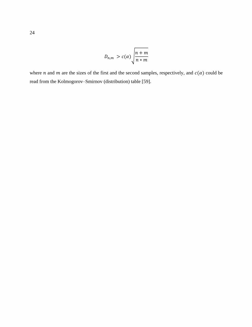
𝐷𝑛,𝑚 > 𝑐(𝛼)√𝑛 + 𝑚

𝑛 ∗ 𝑚

where 𝑛 and 𝑚 are the sizes of the first and the second samples, respectively, and 𝑐(𝛼) could be

read from the Kolmogorov–Smirnov (distribution) table [59].

25

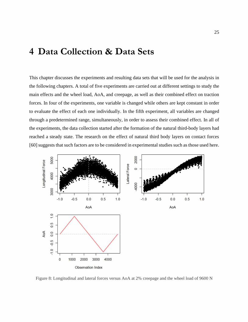
4 Data Collection & Data Sets

This chapter discusses the experiments and resulting data sets that will be used for the analysis in

the following chapters. A total of five experiments are carried out at different settings to study the

main effects and the wheel load, AoA, and creepage, as well as their combined effect on traction

forces. In four of the experiments, one variable is changed while others are kept constant in order

to evaluate the effect of each one individually. In the fifth experiment, all variables are changed

through a predetermined range, simultaneously, in order to assess their combined effect. In all of

the experiments, the data collection started after the formation of the natural third-body layers had

reached a steady state. The research on the effect of natural third body layers on contact forces

[60] suggests that such factors are to be considered in experimental studies such as those used here.

Figure 8: Longitudinal and lateral forces versus AoA at 2% creepage and the wheel load of 9600 N

26

The first data set pertains to the experiment where the longitudinal and lateral forces were

measured continuously at 2% creepage and the wheel load of 9800 N, while sweeping the range

of the AoA from -1 to 1 degrees. The red curve in Figure 8 shows the AoA starting from zero,

linearly increasing to one, linearly going down to -1, and going back to 0 degrees, thereby

completing one positive cycle and one negative cycle. We observe that the longitudinal force varies

non-linearly with the AoA and is symmetric about zero like a quadratic polynomial, whereas the

lateral force slopes upward, resembling a cubic polynomial with a turning point in the middle

where the curvature changes its direction.

Figure 9: Continuous measurement of longitudinal and lateral forces at 0 degrees AoA and 9600 N wheel

load while sweeping the creepage from 0 to 2%

The second data set corresponds to the continuous measurement of the longitudinal and lateral

forces while changing the creepage, as shown in Figure 9. The wheel load in this experiment was

set at 9800 N and the AoA at 0 degrees. The creepage in the second experiment varies linearly in

one and a quarter cycles, as illustrated in the green curve of Figure 9. We note that the longitudinal

27

force slopes up steeply and then flattens out as the creepage gets closer to 2%, while the lateral

force slopes upward linearly and not so steeply. There is also a sharp difference between the range

of the traction forces. The longitudinal force varies between 0 to above 5000 N, whereas the lateral

force does not exceed 1000 N.

The third experiment measures only the longitudinal force but by changing the creepage

incrementally at the following values:

• 0.12%

• 0.25%

• 0.50%

• 1.00%

• 2.00%

Figure 10 shows the measured longitudinal force at various increments of creepage at 0 degrees

AoA and the wheel load of 9600 N. We can see that the discrete measurement of the longitudinal

force progresses following a trend very similar to that of the continuous measurement.

Figure 10: Measured longitudinal force at various increments of creepage at

0 degrees AoA and the wheel load of 9600 N

The fourth data set belongs to measurements of the traction forces at four different wheel loads:

1500 N, 2700 N, 4500 N, and 9800 N, as shown in Figure 11. This figure shows a nice linear

relationship between the longitudinal force and the wheel load. In contrast, the lateral force appears

to progress along a fat line as the wheel load increases.

28

Figure 11: Measurements of longitudinal and lateral forces at 0 degrees AoA and 2% creepage while

incrementally increasing the wheel load

Finally, the last data set measures the traction forces while changing the AoA, creepage, and wheel

load simultaneously. In this data set, the AoA and creepage vary continuously while the wheel

load varies incrementally. The rows of Figure 12 show the measurement of the longitudinal and

lateral forces versus the AoA, creepage, and wheel load, respectively. This experiment was carried

out specifically for the purpose of developing multiple regression models. Creating variation in

the explanatory variables, at least a bigger proportion of them, accommodates the necessary

condition for collecting data that is beyond the simple superposition of the main effects or isolated

data sets and could be used to develop multiple regression models.

The data sets are divided into training and testing sets. The training set will be used to learn

regression models, and the testing sets are used to evaluate the out-of-sample performance of the

trained models. The next chapter employs the first four data sets (and the corresponding training

and testing sets) to study the main effects of the AoA, creepage, and wheel load in isolation and to

develop single regression models.

29

Figure 12: Measurements of longitudinal and lateral forces while changing AoA and creepage

continuously at various wheel load increments

30

5 Single Regression Models and Inference on

the Main Effects of Explanatory Variables

This chapter evaluates the relationship between longitudinal and lateral traction and the wheel-rail

factors that affect the contact forces, namely the angle of attack (AoA), creepage, and the wheel

load. To develop a multiple regression model that involves these variables, one needs to first study

the main effect of each on traction, independent of the others, and find the functional form that

best describes the relationship between them. The extracted features are then combined into a

multiple regression model, and any pairwise interaction between the variables are examined via

model selection methods. The single models are dealt with in this chapter, and multiple models

will be introduced in the following chapter. The analyses in this chapter are conducted within the

classical linear regression framework and using the training data sets. The statistical programming

and computations throughout this thesis are done using R, an open-source programming language

and environment commonly used for statistical computing [61], and its supporting libraries.

5.1 Regressing Longitudinal Force on Angle of Attack (AoA)

This section studies the main effect of the angle of attack on the longitudinal force. The

experimental data pertaining to measuring the longitudinal force while sweeping the range of AoA

from – 1 to 1 degree at 2% creepage and the wheel load of 9600 N was used for this analysis.

5.1.1 Polynomial Regression Model

As shown in Figure 8 of Chapter 4, the longitudinal force varies non-linearly with AoA. The

longitudinal force seems to be symmetrical around zero and slopes downward as the AoA moves

in either direction. Subsequently, the longitudinal force was regressed on AoA using a quadratic

polynomial. The summary of the regression model is shown in Table 2.

31

𝐿𝑜𝑛𝑔𝑖𝑡𝑢𝑑𝑖𝑛𝑎𝑙 𝐹𝑜𝑟𝑐𝑒𝑖 = 𝛽0 + 𝛽1𝐴𝑜𝐴𝑖 + 𝛽2𝐴𝑜𝐴𝑖2 + 𝜀𝑖 𝑤ℎ𝑒𝑟𝑒 𝜀𝑖~𝒩(0, 𝕀2𝜎2)

Table 2: Regression summary for regressing longitudinal force on AoA using a quadratic polynomial

Longitudinal Force

Predictors Estimates CI p

(Intercept) 4529.93 4518.90 – 4540.96 <0.001

AoA 69.34 56.59 – 82.08 <0.001

AoA2 -1093.61 -1118.24 – -1068.98 <0.001

Observations 3360

R2 / R2 adjusted 0.696 / 0.696

5.1.2 Analysis of Residuals

The studentized residuals versus the fitted values are plotted to determine whether the assumptions

of the classical linear regression model hold. More specifically, we determine whether the residuals

of the model are centered around zero, and also whether the homoscedasticity assumption holds

or is violated. It should be noted that the residuals are studentized since we don’t have the true

variance and we are estimating it using the sample. In a similar vein, the histogram and the normal

Q-Q plot are used to determine whether the normality of idiosyncratic noise, as assumed in the

classical linear regression model, is satisfied. These three plots, along with the regression line

plotted on top of the original data, are arranged in a group of four panels in a single figure, and

this scheme will be maintained throughout this document to analyze the residuals of different

regression models. Figure 13 shows these plots for the proposed polynomial regression model.

32

Figure 13: Regressing longitudinal force on AoA using a quadratic polynomial, (upper left panel)

longitudinal force versus AoA and the fitted regression line (upper right panel) studentized residuals vs.

fitted values (lower left panel), and normal Q-Q plot of residuals (lower right) histogram of residuals

As illustrated in the upper right panel of Figure 13, the residuals are centered around zero, and

even though the cloud of the points is denser on the right side, the variance could be considered to

be constant. Taking a closer look, we observe that the fitted curve peaks at zero so a second model

with only a quadratic term was fitted to the data to determine if it makes any significant difference

to the variability captured by the model. Table 3 shows the summary of the second regression

model.

33

𝐿𝑜𝑛𝑔𝑖𝑡𝑢𝑑𝑖𝑛𝑎𝑙 𝐹𝑜𝑟𝑐𝑒𝑖 = 𝛽0 + 𝛽1𝐴𝑜𝐴𝑖2 + 𝜀𝑖 𝑤ℎ𝑒𝑟𝑒 𝜀𝑖~𝒩(0, 𝜎2)

Table 3: Regression summary for regressing longitudinal force on AoA-squared

Longitudinal Force


(Intercept) 4529.31 4518.09 – 4540.52 <0.001

AoA2 -1093.06 -1118.10 – -1068.02 <0.001

Observations 3360

R2 / R2 adjusted 0.686 / 0.686

The coefficient of determination or R2 of the models are very close, and the linear term doesn’t

seem to influence the goodness of fit even though it is statistically significant in the first model.

Nevertheless, the confidence interval in the latter model is tighter compared to the former. It should

be noted that the variability captured by the models would have been higher if there was less

inherent variability in the data and the observations were more concentrated around the fitted line.

The behavior of the residuals provides a better means to compare the models. The residuals in the

scatter plot of Figure 14 are more evenly distributed compared to that of Figure 13, and by

removing the linear term, the behavior of the tails in the normal Q-Q plot (lower left panel of

Figure 14) improves and follows a normal distribution almost perfectly.

Overall, the second model conforms to the assumptions of the classical linear regression model to

a higher degree, is simpler, and captures almost as much of the variability in the data as the first

model; thus, it is a better choice for explaining the relationship between the AoA and the

longitudinal force.

34

Figure 14: Regressing longitudinal force on AoA using only the quadratic term

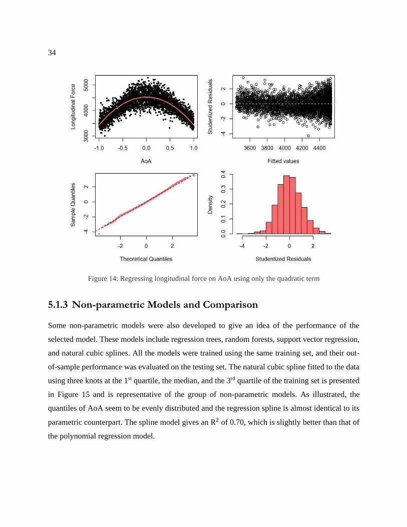
5.1.3 Non-parametric Models and Comparison

Some non-parametric models were also developed to give an idea of the performance of the

selected model. These models include regression trees, random forests, support vector regression,

and natural cubic splines. All the models were trained using the same training set, and their out-

of-sample performance was evaluated on the testing set. The natural cubic spline fitted to the data

using three knots at the 1st quartile, the median, and the 3rd quartile of the training set is presented

in Figure 15 and is representative of the group of non-parametric models. As illustrated, the

quantiles of AoA seem to be evenly distributed and the regression spline is almost identical to its

parametric counterpart. The spline model gives an R2 of 0.70, which is slightly better than that of

the polynomial regression model.

35

Figure 15: Natural cubic spline model for regressing longitudinal force on AoA, vertical lines show the

1st, median, and the 3rd quantiles of AoA respectively

Figure 16 shows the root-mean-squared-error (RMSE) of the predictions on the testing set for all

models. The support vector regression model and the spline model outperform the others;

nonetheless, the magnitude of difference in RMSE across models is very small as to be almost

negligible, approximately 10 N.

Figure 16: Out-of-sample performance of the models for regressing longitudinal force on AoA

36

By and large, it could be concluded that the quadratic polynomial model performs almost as well

as its non-parametric counterparts, both in-sample and out-of-sample.

5.2 Regressing Lateral Force on Angle of Attack (AoA)

This section investigates the main effect of the angle of attack on the lateral force using the same

data sets as the previous section.


We saw in Chapter 4 that the lateral force varies non-linearly with the AoA. The pattern in the data

resembles a cubic polynomial, so different versions of cubic polynomials were compared in a

manner similar to the analysis presented in the previous section. The results showed (not presented

here to avoid redundancy) that the quadratic term in the polynomial does not have much influence

on the performance of the model. The best model based on the comparison is as follows:

𝐿𝑎𝑡𝑒𝑟𝑎𝑙 𝐹𝑜𝑟𝑐𝑒𝑖 = 𝛽0 + 𝛽1𝐴𝑜𝐴𝑖 + 𝛽2𝐴𝑜𝐴𝑖3 + 𝜀𝑖 𝑤ℎ𝑒𝑟𝑒 𝜀𝑖~𝒩(0, 𝕀2𝜎2)

Table 4: Regression summary for regressing lateral force on AoA using a cubic polynomial

Lateral Force


(Intercept) -897.81 -911.13 – -884.50 <0.001

AoA 4717.93 4660.28 – 4775.59 <0.001

AoA3 -1468.62 -1557.04 – -1380.20 <0.001

Observations 3360

R2 / R2 adjusted 0.969 / 0.969

Table 4 shows the regression summary for the proposed model. The model captures as much as

97% of the variability in the data and the coefficient estimates are significant at less than 1% level.

37

Therefore, the next step is to check whether the assumptions of the classical linear regression

model hold.


The scatterplot and normal Q-Q plots in Figure 17 show that we have issues with non-constant

variance and the normality of noise assumptions. The distribution of the residuals has heavier tails

than that of the normal distribution, with the right tail being heavier than the left. We try to resolve

the issues using different transformations.

Figure 17: Regression line and residual plots for regressing the lateral force on creepage using a cubic

polynomial

Figure 18 demonstrates the results of applying various transformations to the response and

explanatory variables. As illustrated, none of the transformations managed to work out the issue

with heteroscedasticity. In other words, the issue couldn’t be rectified using the transformations,

and this leaves us with no other choice but to try to find the closest proxy model.

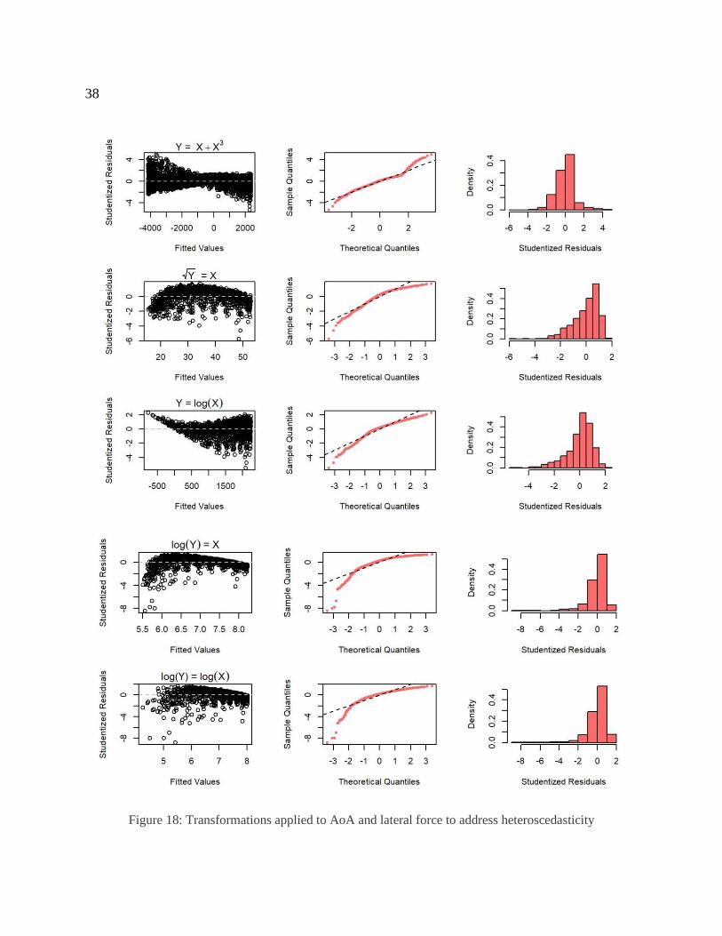
38

Figure 18: Transformations applied to AoA and lateral force to address heteroscedasticity

39

It might also be helpful to entertain a simple linear model and determine how well it performs in

terms of meeting the assumptions, and also to compare the linear and polynomial regression

models with non-parametric models. The results are presented in the following sections.

5.2.3 Linear Model and Assumptions Check

The regression summary and the residual plots for the following linear model are presented in

Table 5 and Figure 19, respectively.

𝐿𝑎𝑡𝑒𝑟𝑎𝑙 𝐹𝑜𝑟𝑐𝑒𝑖 = 𝛽0 + 𝛽1𝐴𝑜𝐴𝑖 + 𝜀𝑖 𝑤ℎ𝑒𝑟𝑒 𝜀𝑖~𝒩(0, 𝜎2)

Table 5: Regression summary for regressing lateral force on AoA

Lateral Force


(Intercept) -893.83 -909.10 – -878.56 <0.001

AoA 3842.11 3815.36 – 3868.86 <0.001

Observations 3360

R2 / R2 adjusted 0.959 / 0.959

The model captures almost as much of the variability in the data as the cubic polynomial, and the

behavior of the tails slightly improves and gets closer to the theoretical normal distribution;

however, a pattern shows up in the scatterplot and the issue with the heteroscedasticity remains

the same.

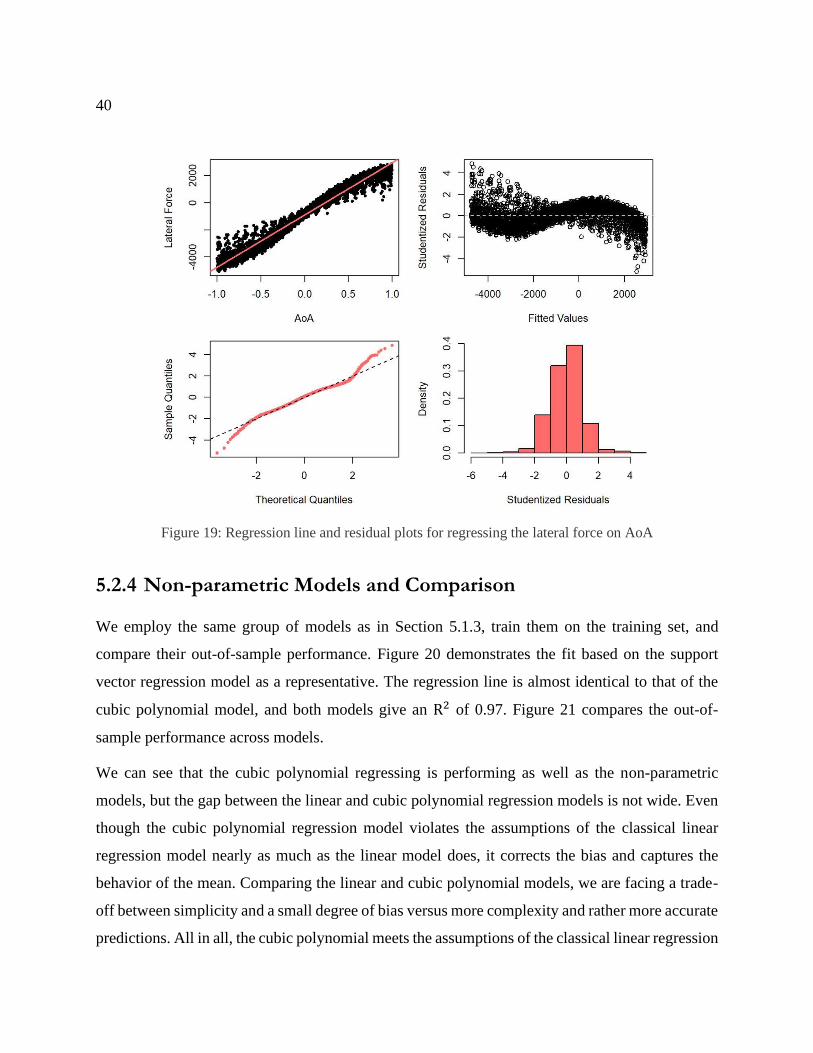
40

Figure 19: Regression line and residual plots for regressing the lateral force on AoA

5.2.4 Non-parametric Models and Comparison

We employ the same group of models as in Section 5.1.3, train them on the training set, and

compare their out-of-sample performance. Figure 20 demonstrates the fit based on the support

vector regression model as a representative. The regression line is almost identical to that of the

cubic polynomial model, and both models give an R2 of 0.97. Figure 21 compares the out-of-

sample performance across models.

We can see that the cubic polynomial regressing is performing as well as the non-parametric

models, but the gap between the linear and cubic polynomial regression models is not wide. Even

though the cubic polynomial regression model violates the assumptions of the classical linear

regression model nearly as much as the linear model does, it corrects the bias and captures the

behavior of the mean. Comparing the linear and cubic polynomial models, we are facing a trade-

off between simplicity and a small degree of bias versus more complexity and rather more accurate

predictions. All in all, the cubic polynomial meets the assumptions of the classical linear regression

41

model to a greater extent and does not suffer from bias, thus, it is a better choice compared to the

linear model.

Figure 20: Support vector regression model for regressing lateral force on AoA

Figure 21: Out-of-sample performance of the models for regressing lateral force on AoA

42

5.3 Regressing Longitudinal Force on Creepage

The analysis in this section is conducted based on the continuous measurement of the longitudinal

force sweeping the range of the creepage from 0 to 2% at the wheel load of 9600 N and the AoA

of 0 degrees.


We have seen in Chapter 4 that there is a non-linear pattern in the data when plotting the

longitudinal force versus creepage, and a quadratic polynomial appears to be the first natural

choice considering the upward sloping trend that flattens out as the creepage increases. The

regression equation and the regression summary table for a quadratic polynomial regression are

presented in the following.

𝐿𝑜𝑛𝑔𝑖𝑡𝑢𝑑𝑖𝑛𝑎𝑙 𝐹𝑜𝑟𝑐𝑒𝑖 = 𝛽0 + 𝛽1𝐶𝑟𝑒𝑒𝑝𝑎𝑔𝑒𝑖 + 𝛽2𝐶𝑟𝑒𝑒𝑝𝑎𝑔𝑒𝑖2 + 𝜀𝑖 𝑤ℎ𝑒𝑟𝑒 𝜀𝑖~𝒩(0, 𝕀2𝜎2)

Table 6: Regression summary for regressing longitudinal force on creepage

Longitudinal Force


(Intercept) 328.86 305.08 – 352.64 <0.001

Creepage 6207.62 6150.21 – 6265.04 <0.001

Creepage2 -2068.99 -2097.37 – -2040.61 <0.001

Observations 4200

R2 / R2 adjusted 0.961 / 0.961

The model explains 96% percent of the variance in the data, and all the estimates for the

coefficients are significant at less than a 1% level. However, before making conclusions about the

goodness of fit, we need to ensure that the assumptions of the classical linear regression model

hold and this may be determined by looking at the residuals.

43


As illustrated in Figure 22, the model suffers from the non-constant variance and there is a non-

linear pattern in the residuals. Nonetheless, there is no major issue with the normality assumption

even though the right tail of the distribution is slightly heavier than that of the theoretical normal

distribution.

To address the non-linearity remaining in the residual, we try other functional forms in our

regression model. Figure 23 compares several such functions, as well as a locally-linear function

(the cut-off was chosen by clustering via GMM4) with the quadratic polynomial introduced earlier.

Figure 22: Regression line and residual plots for regressing the longitudinal force on creepage using a

quadratic polynomial

4 Gaussian Mixture Model

44

As evident, none of the functions could resolve the issue with the non-linearity. Several other

functions were also applied (results not presented here), but none were able to capture the non-

linear pattern completely. Overall, the quadratic polynomial does a better job than other functional

forms in terms of capturing the non-linear pattern in the residuals.

Figure 23: Non-linear functions used to regress longitudinal force on creepage

45

Figure 24: Transformations applied to creepage and longitudinal force to fix heteroscedasticity

46

To fix the heteroscedasticity, we apply transformations to the explanatory variables and the

response. Log transformation is typically used on such occasions and the results of applying it to

our data set are presented in Figure 24. We observe that taking the logarithm of the response, in

our case, the longitudinal force, resolves the non-constant variance; however, it heavily skews the

distribution of the residuals and makes the non-linear pattern stronger.

Comparing the log-transformation and the quadratic polynomial, the latter appears to be a more

plausible model since the normality assumption is met and the non-linearity in the residuals is not

as strong as in the log-transformed model. Here, we don’t have a strong model satisfying all the

assumptions of the linear regression, as was the case with the longitudinal and the AoA, but we

can consider the polynomial (quadratic) regression model as a decent proxy. In the next section,

we explore non-parametric methods and attempt to make a comparison with our proxy model.

5.3.3 Comparison with Non-parametric Models

Figure 25 shows the fitted natural cubic spline to the data along with the plots for the residuals.

Here again, the 1st quartile, the median, and the 3rd quartile were chosen as knots. The spline gives

an R2 of 0.98 and we observe that the spline captures all the non-linearity in the residuals, but the

variance increases as we move along the fitted values, and the residuals have heavier tails than that

of a theoretical normal distribution. This suggests that even though the quadric polynomial model

is slightly biased (does not follow the mean perfectly), which leaves some degree of non-linearity

in the residuals, the residuals follow the theoretical normal distribution more closely than an

unbiased model, i.e., a natural cubic spline. The results from the support vector regression that

models the data points as univariate normal are almost identical to that of the spline, so the results

are not presented separately.

47

Figure 25: Natural cubic spline and residual plots for regressing longitudinal force on creepage

Figure 26: Out-of-sample performance of the models for regressing longitudinal force on creepage

Figure 26 shows the root-mean-squared-error (RMSE) of the predictions on the testing set for the

non-parametric models including regression trees, random forests, support vector regression, and

48

natural cubic splines. All these models outperform the polynomial regression model in terms of

out-of-sample prediction accuracy, and the difference in RMSE on the testing set is roughly 70 N

or about 35 percentage points greater than the non-parametric models.

5.3.4 Polynomial Regression Model Trained on Incremental

Measurement

As discussed in Chapter 4, one of the restrictions in running the experiments and in the data

collection stage was the fact that not all of the dependent variables could be measured continuously

at the same time. In other words, the rig allows for the measurement of creepage, and the angle of

attack (AoA) could vary continuously in high precision measurement mode only when the wheel

load varies discretely. This creates a discrepancy in the modes of data collection, specifically for

studying the main effects of wheel load on the longitudinal force.

Figure 27: Regression line and the residuals plots for regressing the longitudinal force on creepage using

discrete measurement data

49

To determine whether if the discrete measurements could act as a good proxy for continuous

measurements, the discrete measurements of the creepage are used to train the same polynomial

regression model for regressing the longitudinal force on the creepage. The discrete data was split

into training and testing sets, and the training set was used to estimate the regression coefficients.

The results are presented in Table 7.

Table 7: Regression summary for regressing longitudinal force on creepage using discrete data

Longitudinal Force


(Intercept) 441.70 426.63 – 456.78 <0.001

Creepage 4798.86 4758.54 – 4839.18 <0.001

Creepage2 -1357.29 -1375.51 – -1339.07 <0.001

Observations 6272

R2 / R2 adjusted 0.964 / 0.964

The coefficient estimates are significant at less than a 1% level and the standard errors are small,

thus making the confidence intervals tight. The point estimates are different from that of the

continuous data set, which stems from the experiment conditions being different during discrete

measurement. At this stage, our emphasis is on choosing the closest functional form that captures

the relationship between the dependent and independent variables, so we are not very concerned

with the point estimates; we are more focused on the predictive power of the model or its out-of-

sample performance. In other words, training the model using different data sets should provide

approximately the same level of accuracy of the predictions if the functional form is close to the

true underlying relationship.

The model trained on the continuous data set returned an RMSE of 270.3 N on the testing set.

Training the same model on the discrete set gives an R2 of 0.96, and making predictions on the

discrete testing set gives an RMSE of 272.89 N. We observe that the performance of the model on

50

the discrete and continuous datasets is nearly the same. This provides another piece of evidence in

support of the proposed polynomial model.

5.4 Regressing Lateral Force on Creepage

This section investigates the main effect of creepage on the lateral force using the same data sets

as used in the previous section. In this case, we should consider the fact that creepage has more to

do with the longitudinal force, while its relation to the lateral force stems from the geometry of the

wheel. More specifically, only a tapered wheel, which was used in our experiments, could create

such an interaction.

5.4.1 Linear Regression Model and Assumptions Check

The following equation formulates a linear relationship between the lateral force and the creepage.

The regression summary and residuals plots for the proposed linear model are presented in Table

8 and Figure 8, respectively.

𝐿𝑎𝑡𝑒𝑟𝑎𝑙 𝐹𝑜𝑟𝑐𝑒𝑖 = 𝛽0 + 𝛽1𝐶𝑟𝑒𝑒𝑝𝑎𝑔𝑒𝑖 + 𝜀𝑖 𝑤ℎ𝑒𝑟𝑒 𝜀𝑖~𝒩(0, 𝜎2)

Table 8: Regression summary for regressing lateral force on creepage

Lateral Force


(Intercept) 458.44 452.68 – 464.21 <0.001

Creepage 124.97 119.54 – 130.40 <0.001

Observations 4200

R2 / R2 adjusted 0.327 / 0.327

The low value of the coefficient of determination, R2, is due to the inherent dispersion in the data.

In other words, the cloud of data points forms a wide band around the regression line that adversely

51

affects the variability captured by the model, and it has nothing to do with the trend that the band

follows.

Figure 28: Regression line and residual plots for regressing the lateral force on creepage

From the scatterplot, we observe that the variance remains constant as we move along the fitted

values, and from the normal Q-Q plot, we see that the distribution of the residuals is very close to

the theoretical normal distribution, except for the left tail which is slightly heavier. Overall, the

assumptions of the classical linear regression model hold to a high degree and we may conclude

that the relationship between the lateral force and creepage could be modeled linearly.

5.5 Regressing Longitudinal Force on Wheel Load

A side conclusion from the results presented in Section 5.3.4 could be that varying the wheel load

incrementally could also act as a good proxy for continuous measurement, and that is the fact that

we will be employing for regressing the longitudinal force on the wheel load. In the corresponding

52

data set, the longitudinal force was measured at four points covering the entire range of the wheel

load, with the AoA being 0 degrees and at 2% creepage. The analysis is presented in the following

sections.


Based on the discussions in the previous chapter, it makes a plausible case to assume that the

longitudinal force varies linearly with the wheel load, so we start with a linear regression model.

Table 9 shows the regression summary and Figure 29 shows the residual plots for the proposed

model:

𝐿𝑜𝑛𝑔𝑖𝑡𝑢𝑑𝑖𝑛𝑎𝑙 𝐹𝑜𝑟𝑐𝑒𝑖 = 𝛽0 + 𝛽1𝐿𝑜𝑎𝑑𝑖 + 𝜀𝑖 𝑤ℎ𝑒𝑟𝑒 𝜀𝑖~𝒩(0, 𝜎2)

Table 9: Regression summary for regressing longitudinal force on wheel load

Longitudinal Force


(Intercept) -185.93 -231.04 – -140.82 <0.001

Load 0.53 0.52 – 0.53 <0.001

Observations 700

R2 / R2 adjusted 0.957 / 0.957

We observe that the estimates are significant, and from the scatter plot we can see that the

homoscedasticity is not violated. Although the distribution of the residuals is slightly left-skewed,

the slight deviation from the normal distribution that we observe in the lower panels of Figure 29

could be attributed to discrete measurement. Comparison with non-parametric methods wouldn’t

be helpful for the main effect of wheel load since such methods model the gap between the discrete

measurements with non-linearity and hence tend to overfit.

53

Figure 29: Regression line and residual plots for regressing the longitudinal force on wheel load

5.6 Regressing Lateral Force on Wheel Load

We take the same approach as the longitudinal force in modeling the lateral force. It is particularly

helpful to consider the mechanics involved in experiments when analyzing the lateral force. We

don’t expect the wheel load to influence the lateral force in a typical wheel-rail contact, specifically

when the wheel is cylindrical. However, a tapered wheel was used in the experiments to create

such an interaction between the two.


Following the line of reasoning in Section 5.6, we expect to see a significant but very small

correlation between the lateral force and the wheel load in the following model. Table 10 shows

the regression summary for the model.

54

𝐿𝑎𝑡𝑒𝑟𝑎𝑙 𝐹𝑜𝑟𝑐𝑒𝑖 = 𝛽0 + 𝛽1𝐿𝑜𝑎𝑑𝑖 + 𝜀𝑖 𝑤ℎ𝑒𝑟𝑒 𝜀𝑖~𝒩(0, 𝜎2)

Table 10: Regression summary for regressing lateral force on wheel load

Lateral Force


(Intercept) 54.17 49.10 – 59.24 <0.001

Load 0.01 0.01 – 0.01 <0.001

Observations 7000

R2 / R2 adjusted 0.047 / 0.047

The estimate for 𝛽1 is 0.01 and it is statistically significant. Nonetheless, the model explains only

4.7% of the variability in the data. These results corroborate our initial intuition about the

relationship between the lateral force and the wheel load.

Figure 30: Regression line and residual plots for regressing the lateral force on wheel load

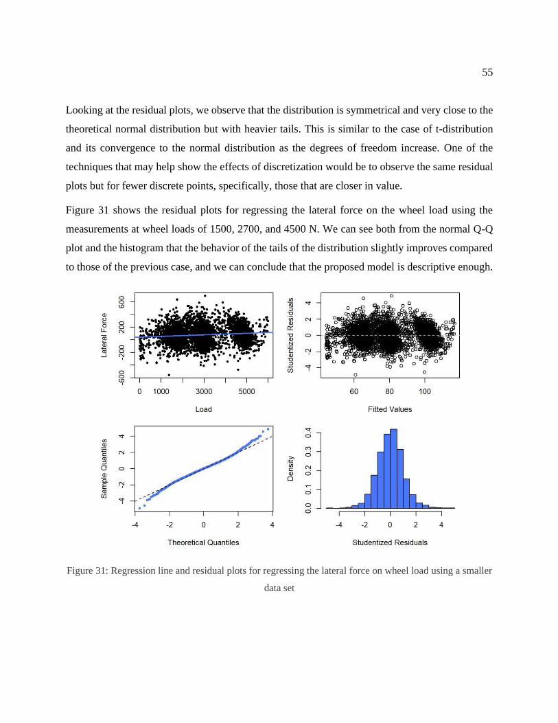
55

Looking at the residual plots, we observe that the distribution is symmetrical and very close to the

theoretical normal distribution but with heavier tails. This is similar to the case of t-distribution

and its convergence to the normal distribution as the degrees of freedom increase. One of the

techniques that may help show the effects of discretization would be to observe the same residual

plots but for fewer discrete points, specifically, those that are closer in value.

Figure 31 shows the residual plots for regressing the lateral force on the wheel load using the

measurements at wheel loads of 1500, 2700, and 4500 N. We can see both from the normal Q-Q

plot and the histogram that the behavior of the tails of the distribution slightly improves compared

to those of the previous case, and we can conclude that the proposed model is descriptive enough.

Figure 31: Regression line and residual plots for regressing the lateral force on wheel load using a smaller

data set

56

6 Multiple Regression Models

This chapter extends the results of the previous chapter from single- to multiple-regression. The

models developed in this chapter not only account for the main effects of wheel load, % creepage,

and AOA, but also the interactions between them. The data set pertaining to the measurement of

traction force while continuously changing the AoA and creepage and incrementally increasing

the wheel load is used throughout the analysis.

There are a number of (implicit) guidelines that would help with extending the single-regression

models to multiple-regression. The first is checking for multicollinearity among the explanatory

variables. Second, the sign of the main effects in the multiple regression model must match the

corresponding single regression model. The latter ensures that the main effect of each explanatory

variable acts in the direction of its true influence on the response, while the former ensures that

none of the columns of (the matrix of) explanatory variables is a linear combination of other

columns. One must note that the key term here is linear. In other words, the correlation matrix

does not reveal anything about the non-linear relationship between any two columns.

Table 11 shows the correlation matrix for the explanatory variables in the data set. We observe

that there are no strong pairwise correlations between the explanatory variables, therefore, there

are no issues in this respect. Match or mismatch of the sign of the main effects in the multiple

regression model may be checked during the model selection process.

Table 11: Pairwise correlation of explanatory variables

Load AoA Creepage

Load 1.00 -0.057 0.002

AoA -0.057 1.00 0.00

Creepage 0.002 0.00 1.00

57

6.1 Multiple Regression Model for Lateral Force

In Chapter 5, we concluded that lateral forces have a small direct linear relationship with the wheel

load and creepage, and a cubic relationship with AoA. We also discussed that the aforementioned

linear relationships make intuitive sense since it is through the AoA that lateral forces are possible.

The wheel load influences the lateral force only through the taper of the wheel. In the following

sections, we attempt to develop a multiple regression model for the lateral force using different

methods.

6.1.1 Superposition of Main Effects

Probably the simplest way of approaching the problem is to take the superimposition of the main

effects as the multiple regression model and determine how it performs in terms of capturing the

variability in the data. This model could also serve as the basis for comparison with more

complicated models. The following equation represents the proposed model.

𝐿𝑎𝑡𝑒𝑟𝑎𝑙 𝐹𝑜𝑟𝑐𝑒𝑖 = 𝛽0 + 𝛽1𝐿𝑜𝑎𝑑𝑖 + 𝛽2𝐶𝑟𝑒𝑒𝑝𝑎𝑔𝑒𝑖 + 𝛽3𝐴𝑜𝐴𝑖 + 𝛽4𝐴𝑜𝐴3𝑖 + 𝜀𝑖

𝑤ℎ𝑒𝑟𝑒 𝜀𝑖~𝒩(0, 𝕀4𝜎2)

Here we are modeling the variation in the data with a multivariate normally-distributed variable

centered at zero and a constant (and equal) variance in all four dimensions of dependent variables.

As discussed in Chapter 3, the assumptions for the multiple regression model remain the same as

for the classical linear regression model, except for their dimensionality. Table 12 presents the

regression summary for the above model. The model gives an R2of 69% with all the coefficients

being statistically significant at less than a 1% level. This suggests that the relation between the

lateral force and the explanatory variables is probably beyond the simple superposition of main

effects, and there possibly exist some interactions among them. We will investigate this using

model selection methods. First, however, it might be helpful to compare how the model would

perform if we incorporated the linear model for the main effect of the AoA on the lateral force.

The regression summary for this model is presented in Table 13.

58

Table 12: Regression summary for regressing lateral force on the main effects of explanatory variables

Lateral Force


(Intercept) 34.19 30.35 – 38.03 <0.001

Load 0.12 0.12 – 0.12 <0.001

AoA 3604.17 3597.45 – 3610.89 <0.001

AoA3 -2221.50 -2231.75 – -2211.24 <0.001

Creepage -35.70 -38.39 – -33.01 <0.001

Observations 1344000

R2 / R2 adjusted 0.695 / 0.695

Table 13: Regression summary for regressing lateral force on the main effects of explanatory variables

(AoA linearly varying with lateral force)

Lateral Force


(Intercept) 40.72 36.63 – 44.80 <0.001

Load 0.12 0.11 – 0.12 <0.001

AoA 2270.89 2268.03 – 2273.76 <0.001

Creepage -35.22 -38.08 – -32.36 <0.001


R2 / R2 adjusted 0.654 / 0.654

We observe that the cubic term accounts for approximately 4% of the variability in the data. In

other words, the cubic term does not appear to be remarkably influential. This observation is

59

compatible with what we saw in Chapter 5 on the low curvature of the fitted line regressing the

lateral force on the AoA using a cubic polynomial.

6.1.2 Stepwise Model Selection via BIC

In terms of the interactions, there are six5 possible combinations of pairwise interactions among

the explanatory variables in our model: wheel load, creepage, AoA, and AoA3. We discussed in

Chapter 3 that the forward stepwise model selection starts from the base model or simply the mean

of the response, adds one term to the model, either main effect or pair-wise interaction at each step,

and continues adding terms until it reaches the model containing all possible interactions. In the

end, it chooses the model with the lowest BIC. Table 14 presents the regression summary for the

model selected using this method.


Lateral Force


(Intercept) -116.18 -117.69 – -114.67 <0.001

AoA 678.31 673.71 – 682.90 <0.001

Load 0.16 0.16 – 0.17 <0.001

AoA3 -511.29 -522.63 – -499.94 <0.001

Creepage -67.55 -68.91 – -66.19 <0.001

AoA * Load 0.72 0.72 – 0.72 <0.001

Load * AoA3 -0.43 -0.43 – -0.43 <0.001

AoA * AoA3 478.81 477.02 – 480.60 <0.001

5 Selection of k items from a collection of size n: (𝑛 = 4𝑘 = 2

) = 6

60

AoA * Creepage -911.84 -916.07 – -907.61 <0.001

AoA3 * Creepage 939.46 933.32 – 945.60 <0.001

Load * Creepage -0.02 -0.02 – -0.02 <0.001


R2 / R2 adjusted 0.977 / 0.977

We can see that the selected model explains almost all the variance (97.7%) in the data, and that

all the coefficient estimates are significant; however, this approach introduces all the possible

pairwise interactions among the explanatory variables to our base model (superposition of main

effects). In other words, this is the most complex model (taking only pairwise interactions into

account) that we could have entertained!

It would be beneficial to bear in mind that BIC is a criterion based on the MLE6 of �̂� and �̂�2 plus

a penalizing factor for the number of variables. This means that the selected model is not

necessarily interpretable. While this method is one of the most widely used methods for model

selection, in our case, it does not help simplify.

We repeat the process for the case of a linear relationship between the lateral force and the AoA

to determine how the model selected under this condition will perform. The regression summary

for the selected model under this condition is presented in Table 15.



Lateral Force


(Intercept) -83.36 -85.54 – -81.18 <0.001

AoA 1231.36 1228.55 – 1234.16 <0.001

6 Maximum Likelihood Estimator

61

Load 0.15 0.15 – 0.15 <0.001

Creepage 3.06 1.18 – 4.95 0.001

AoA * Load 0.46 0.46 – 0.46 <0.001

AoA * Creepage -988.69 -990.54 – -986.85 <0.001

Load * Creepage -0.01 -0.01 – -0.01 <0.001


R2 / R2 adjusted 0.952 / 0.952

Interestingly, the selected model is comprised of six terms and explains almost as much of the

variability in the data as the previously selected model. This paves the way for excluding the cubic

term from the multiple regression models, but before drawing any conclusions, we may cross-

check this result with a similar stepwise selection approach that employs various criteria for

selecting among models.

6.1.3 Best Subset Selection & LASSO

As discussed earlier, the best subset selection chooses a subset of predictors that yields the best

results based on some selection criteria. Figure 32 shows the progression of these criteria during

the selection process. The following are the first four models consecutively:

1. 𝐿𝑎𝑡𝑒𝑟𝑎𝑙 𝐹𝑜𝑟𝑐𝑒𝑖 = 𝛽0 + 𝛽1𝑳𝒐𝒂𝒅𝒊 ∗ 𝑨𝒐𝑨𝒊 + 𝜀𝑖

2. 𝐿𝑎𝑡𝑒𝑟𝑎𝑙 𝐹𝑜𝑟𝑐𝑒𝑖 = 𝛽0 + 𝛽1𝑳𝒐𝒂𝒅𝒊 + 𝛽2𝑳𝒐𝒂𝒅𝒊 ∗ 𝑨𝒐𝑨𝒊 + 𝜀𝑖

3. 𝐿𝑎𝑡𝑒𝑟𝑎𝑙 𝐹𝑜𝑟𝑐𝑒𝑖 = 𝛽0 + 𝛽1𝑳𝒐𝒂𝒅𝒊 + 𝛽2𝑳𝒐𝒂𝒅𝒊 ∗ 𝑨𝒐𝑨𝒊 + 𝛽3𝑳𝒐𝒂𝒅𝒊 ∗ 𝑨𝒐𝑨𝟑𝒊 + 𝜀𝑖

4. 𝐿𝑎𝑡𝑒𝑟𝑎𝑙 𝐹𝑜𝑟𝑐𝑒𝑖 =

𝛽0 + 𝛽1𝑳𝒐𝒂𝒅𝒊 + 𝛽2𝑳𝒐𝒂𝒅𝒊 ∗ 𝑨𝒐𝑨𝒊 + 𝛽3𝑳𝒐𝒂𝒅𝒊 ∗ 𝑨𝒐𝑨𝟑𝒊 + 𝛽4𝑨𝒐𝑨𝒊 ∗ 𝑨𝒐𝑨𝟑

𝒊 + 𝜀𝑖

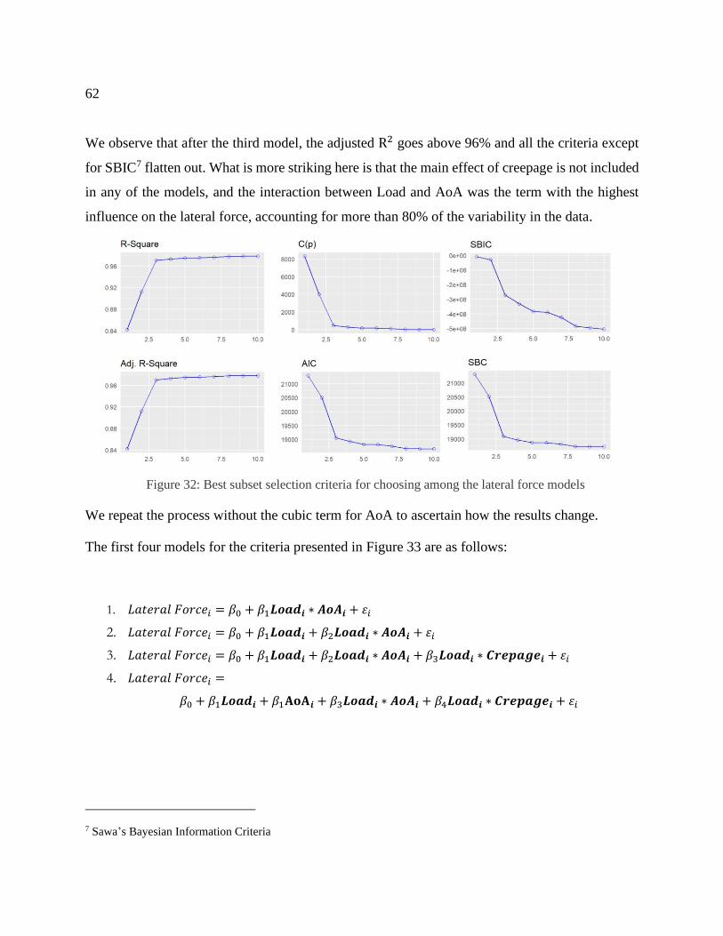
62

We observe that after the third model, the adjusted R2 goes above 96% and all the criteria except

for SBIC7 flatten out. What is more striking here is that the main effect of creepage is not included

in any of the models, and the interaction between Load and AoA was the term with the highest

influence on the lateral force, accounting for more than 80% of the variability in the data.

We repeat the process without the cubic term for AoA to ascertain how the results change.

The first four models for the criteria presented in Figure 33 are as follows:

1. 𝐿𝑎𝑡𝑒𝑟𝑎𝑙 𝐹𝑜𝑟𝑐𝑒𝑖 = 𝛽0 + 𝛽1𝑳𝒐𝒂𝒅𝒊 ∗ 𝑨𝒐𝑨𝒊 + 𝜀𝑖

2. 𝐿𝑎𝑡𝑒𝑟𝑎𝑙 𝐹𝑜𝑟𝑐𝑒𝑖 = 𝛽0 + 𝛽1𝑳𝒐𝒂𝒅𝒊 + 𝛽2𝑳𝒐𝒂𝒅𝒊 ∗ 𝑨𝒐𝑨𝒊 + 𝜀𝑖

3. 𝐿𝑎𝑡𝑒𝑟𝑎𝑙 𝐹𝑜𝑟𝑐𝑒𝑖 = 𝛽0 + 𝛽1𝑳𝒐𝒂𝒅𝒊 + 𝛽2𝑳𝒐𝒂𝒅𝒊 ∗ 𝑨𝒐𝑨𝒊 + 𝛽3𝑳𝒐𝒂𝒅𝒊 ∗ 𝑪𝒓𝒆𝒑𝒂𝒈𝒆𝒊 + 𝜀𝑖

4. 𝐿𝑎𝑡𝑒𝑟𝑎𝑙 𝐹𝑜𝑟𝑐𝑒𝑖 =

𝛽0 + 𝛽1𝑳𝒐𝒂𝒅𝒊 + 𝛽1𝐀𝐨𝐀𝒊 + 𝛽3𝑳𝒐𝒂𝒅𝒊 ∗ 𝑨𝒐𝑨𝒊 + 𝛽4𝑳𝒐𝒂𝒅𝒊 ∗ 𝑪𝒓𝒆𝒑𝒂𝒈𝒆𝒊 + 𝜀𝑖

7 Sawa’s Bayesian Information Criteria

Figure 32: Best subset selection criteria for choosing among the lateral force models

63

The first two models are the same; however, the creepage shows up in interaction terms instead of

AoA3 in the third and the fourth models. Another fact that is consistent across all panels in Figure

33 is that all the criteria completely flatten out after the fourth model. These results suggest that

AoA3 and creepage do not explain much variability in the data, so they could be excluded from our

model. Before dropping these variables, we may check the least important variable(s) using

shrinkage methods, e.g., the Least Absolute Shrinkage and Selection Operator (LASSO).

Here, we are feeding the model with all pairwise interactions to the algorithm to determine which

explanatory variables will be left out during the shrinkage process. Table 16 and

Table 17 shows the coefficients estimated by LASSO for the model, including AoA3 in main effects

and all possible interaction terms and without AoA3, respectively.

Table 16: LASSO coefficient estimates for the lateral force model including AoA3 and its interactions

Variable Load AoA Creepage 𝐀𝐨𝐀𝟑 AoA*Load AoA*Creepage Creepage*Load 𝐀𝐨𝐀𝟑*Load 𝐀𝐨𝐀𝟑*Creepage

Estimate 0.29 0.11 0.00 0.00 1.42 -0.16 -0.018 -0.55 0.076

Figure 33: Best subset selection criteria for choosing among the lateral force models


64

Table 17: LASSO coefficient estimates for the lateral force model excluding AoA3 and its interactions

Variable Load AoA Creepage AoA*Load AoA*Creepage Creepage*Load

Estimate 0.26 0.33 0.00 0.91 -0.34 0.00

In Table 16, the coefficient estimates for creepage and AoA3 are zero and we have the same

situation with the creepage and its interactions with the wheel load in

Table 17. These results are in line with those from that of subset selection; hence, we can conclude

that the AoA3 and the main effect of creepage could be excluded from the multiple regression model

for the lateral force.

Despite model selection via BIC, the best subset selection approach helped simplify the model to

some extent while maintaining the in-sample performance of the model roughly on the same level

as the more complicated models. Nevertheless, we cannot make any confident conclusions about

the best model based on these results. One way to bridge this gap is to take a multi-faceted

approach and attempt to compare the results from various methods. On this basis, principle

component analysis could be a good complement to the results that we already have obtained.

6.1.4 Principal Component Analysis and the Importance of Variables

The principal component analysis is typically used for dimensionality reduction and choosing the

dimensions that explain the highest proportions of variance. Figure 34 shows the percentage of

variance explained by the main effects and their pairwise interactions, excluding the AoA3 and its

interactions across the principal components (or dimensions).

We observe that more than 90% of the variance is explained by the first three components. This

proportion is compatible with what we have seen in subset selection. The important factor at this

stage is the contribution of the explanatory variables to each component. In other words, we are

interested in the explanatory variables with the highest contributions to the first few principal

components.

65

Figure 34: Percentage of variance explained by the main effects and their pairwise interactions, excluding

the AoA3 and its interactions across the principal components

Figure 35 and Figure 36 illustrate the contribution of the main effects and their pairwise

interactions (excluding AoA3 and its interactions) to the first and the second principal components,

respectively.

AoA and its interaction with the wheel load and creepage make up the first component, while the

second component is comprised of the interaction of creepage and wheel load, wheel load, and

creepage in the order of their contributions. It may be helpful to review the direction and magnitude

of the contribution of these variables to the first two components, as shown in Figure 37. The AoA

and its interactions are perfectly aligned with the first component, but this is not the case with the

variables contributing to the second component. The interaction of creepage and the wheel load is

perfectly aligned with the second dimension, but there is a degree of misalignment for the wheel

and creepage.

66

Figure 35: Contribution of main effects and their pairwise interactions to the first principal component

(excluding AoA3 and its interactions)

Figure 36: Contribution of main effects and their pairwise interactions to the second principal component

(excluding AoA3 and its interactions)

67

Based on Figure 36, one can draw inference about the variables of interest entirely based on

analysis and without having any intuition about the underlying process. In other words, we can

argue that the AoA is the most important variable in determining the lateral force from a purely

mathematical point of view. On the other hand, wearing our mechanical engineering hat, we know

that this makes perfect sense since it is through the AoA that steering is possible.

Figure 37: Polar plot for the contribution of the main effects and their pairwise interactions to the first and

second principal component

Figure 38 shows the relative importance of explanatory variables in a random forest model based

on a measure, namely node impurity. “In each tree in the forest, whenever we select a variable and

perform a split, the impurity is decreased. Therefore, one way to measure the importance of a

variable is to average the reduction in impurity, taken over all the times that variable is selected

for splitting in all of the trees in the forest” [55]. Here, we are not concerned with the details of

developing a non-parametric model, such as a random forest, but rather we use it as a

complementary measure to help us draw inferences. We can see that the order of importance makes

68

intuitive sense, with the AoA being the most important and creepage the least important, and is

consistent with the contribution of the variables to the first principle component.

Figure 38: Importance of variables in the random forest model of lateral force based on the average

decrease in node impurity

Continuing with this line of reasoning, we can argue that creepage is the least important variable

as far as the first two principal components are concerned. This is also consistent with the results

from LASSO (creepage was estimated to be 0.00) and subset selection. Summing up, we are left

with the following explanatory variables for our multiple regression model:

• AoA

• AoA*Load

• AoA*Creepage

• Load*Creepage

• Load

6.1.5 Selected Model

Of the remaining variables, the interaction of creepage and the wheel load is the most arguable

since it was dropped by LASSO, whereas it had the highest contribution to the second component

in the PCA and also showed up in the third and the fourth models in the subset selection. The high

69

contribution of this term to the second principal component could be due to either the significance

of creepage, which is doubtful, or simply the intensified effect of wheel load when multiplied by

the creepage. Either way, evaluating the models containing this term will clarify the matter. Table

18 presents the adjusted R2 for the models containing the interaction of creepage and the wheel

load.

Table 18: Adjusted R2 for the models incorporating the interaction of creepage and the wheel load

Lateral Force Model Adjusted 𝐑𝟐

Load + AoA 65.8 %

Load + AoA + Creepage*Load 65.8 %

Load + AoA + Creepage*Load + AoA*Creepage 69.5 %

Load + AoA + AoA*Load 91.3 %

We observe that the model containing this term is no different than for the main effects of the

wheel load and AoA, thus corroborating the results of LASSO.

Eventually, we are left with two rational choices for the multiple regression model of the lateral

force. These choices along with their respective regression summaries are presented in Table 19

and Table 20, respectively.

𝐿𝑎𝑡𝑒𝑟𝑎𝑙 𝐹𝑜𝑟𝑐𝑒𝑖 = 𝛽0 + 𝛽1𝐿𝑜𝑎𝑑𝑖 + 𝛽2𝐴𝑜𝐴𝑖 + 𝛽3𝐿𝑜𝑎𝑑𝑖 ∗ 𝐴𝑜𝐴𝑖 + 𝜀𝑖


Table 19: Regression summary for the first alternative for modeling lateral force

Lateral Force


(Intercept) -80.66 -127.84 – -33.48 0.001

Load 0.14 0.13 – 0.15 <0.001

AoA 84.10 3.32 – 164.87 0.041

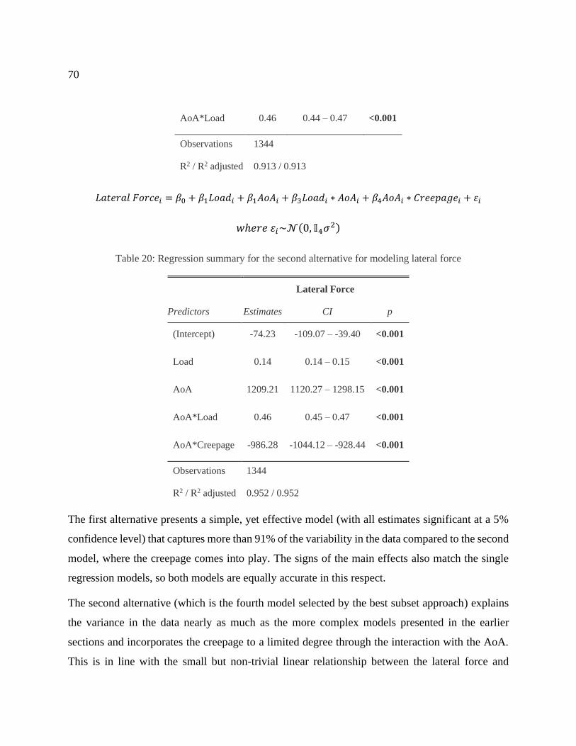
70

AoA*Load 0.46 0.44 – 0.47 <0.001

Observations 1344

R2 / R2 adjusted 0.913 / 0.913

𝐿𝑎𝑡𝑒𝑟𝑎𝑙 𝐹𝑜𝑟𝑐𝑒𝑖 = 𝛽0 + 𝛽1𝐿𝑜𝑎𝑑𝑖 + 𝛽1𝐴𝑜𝐴𝑖 + 𝛽3𝐿𝑜𝑎𝑑𝑖 ∗ 𝐴𝑜𝐴𝑖 + 𝛽4𝐴𝑜𝐴𝑖 ∗ 𝐶𝑟𝑒𝑒𝑝𝑎𝑔𝑒𝑖 + 𝜀𝑖


Table 20: Regression summary for the second alternative for modeling lateral force

Lateral Force


(Intercept) -74.23 -109.07 – -39.40 <0.001

Load 0.14 0.14 – 0.15 <0.001

AoA 1209.21 1120.27 – 1298.15 <0.001

AoA*Load 0.46 0.45 – 0.47 <0.001

AoA*Creepage -986.28 -1044.12 – -928.44 <0.001

Observations 1344

R2 / R2 adjusted 0.952 / 0.952

The first alternative presents a simple, yet effective model (with all estimates significant at a 5%

confidence level) that captures more than 91% of the variability in the data compared to the second

model, where the creepage comes into play. The signs of the main effects also match the single

regression models, so both models are equally accurate in this respect.

The second alternative (which is the fourth model selected by the best subset approach) explains

the variance in the data nearly as much as the more complex models presented in the earlier

sections and incorporates the creepage to a limited degree through the interaction with the AoA.

This is in line with the small but non-trivial linear relationship between the lateral force and

71

creepage in the single regression model for the main effect of the creepage on the lateral force. In

addition, the coefficient estimates are significant at less than a 1% confidence level. These factors

make the second alternative the strongest candidate for modeling the lateral force.

In summary, the selected multiple regression model suggests that the relationship among the

variables is beyond the superposition of main effects.

6.2 Distribution of Predictions for Multiple Regression Model

of Lateral Force

In Chapter 5, we dealt with the main effects of explanatory variables. Some of these models

satisfied the assumptions of the classical linear regression model while others did not. Failing to

meet the assumptions in all single models is important since it affects how the uncertainty of

predictions is quantified. More specifically, the point estimates or predictions made by such a

multiple regression model are valid since a linear operator was expected, regardless of the variance

of the variable. This, however, is not the case with the confidence and prediction intervals

especially when the variance is not constant in the single models.

Figure 39 shows the predictions made by the multiple regression model on the testing set versus

the true values, along with the 95% confidence interval of predictions. The mean closely (but not

perfectly) follows the true values, and the confidence interval of predictions is very tight. The

multiple regression model exhibits very low bias and only at some points across the range of

predictions. However, we have no idea how reliable the confidence interval of predictions is since

not all the assumptions of the linear regression model were met by the single models. To address

this issue, we attempt to develop an unbiased (as much as possible) non-parametric model and

empirically obtain the distribution of the predictions by bootstrapping over the residuals. This

approach allows us to compare the distribution of predictions from this model with that of the

multiple regression model to determine the extent of the difference between the two.

72

Figure 39: Multiple regression model for lateral force, predictions and 95% confidence interval of

predictions

Figure 40 shows the mean and the 95% prediction interval of the predictions made by the

developed support vector multiple regression model. The model was trained on the training set and

predictions were made on the testing set. We can see that the prediction mean almost perfectly

follows the true values, and the confidence interval of predictions is very tight, as was the case

with the multiple regression model. There are different ways to compare two distributions, but for

simplicity, we only compare the upper and the lower bounds of the 95% confidence interval of

predictions from both models.

-

73

Figure 40: SVR model for lateral force, predictions and 95% confidence interval of predictions

Figure 41 and Figure 42 illustrate the CDF8 and the density plots for the upper and the lower

bounds of the 95% confidence interval of the prediction on the testing set for both models. We

observe that for both cases, the distributions are very close, as none of the models have first-order

stochastic dominance over the others. We could also statistically check the equality of the two

distributions using the Kolmogorov-Smirnov Test.

8 Cumulative Density Function

-

74

Figure 41: Empirical CDF and density plot of the lower bounds of the 95% confidence interval of

predictions from the multiple regression model and the SVR model

Den

sity

Lateral Force

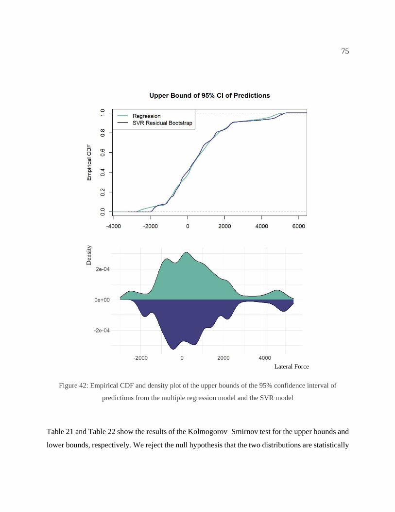
75

Figure 42: Empirical CDF and density plot of the upper bounds of the 95% confidence interval of

predictions from the multiple regression model and the SVR model

Table 21 and Table 22 show the results of the Kolmogorov–Smirnov test for the upper bounds and

lower bounds, respectively. We reject the null hypothesis that the two distributions are statistically

Den

sity

Lateral Force

76

identical at a 1% confidence level for both cases. However, even though the tests show that neither

the upper bounds nor the lower bounds of the confidence intervals of the predictions are

statistically equal, from the test statistic, we can see that the difference between them is not

substantial. On this basis, we can argue that even though the assumptions of the classical linear

regression model do not completely hold, the multiple regression model does a decent job, and the

results are accurate enough to serve as a proxy for the true underlying model.


predictions from the multiple regression model of lateral force and the SVR model

Two-sample Kolmogorov-Smirnov Test

D = 0.053819, p-value = 1.136e-07

Alternative hypothesis: two-sided


predictions from the multiple regression model of lateral force and the SVR model


D = 0.046007, p-value = 1.014e-05


6.3 Multiple Regression Model for Longitudinal Force

In Chapter 5, we concluded that the longitudinal force has a linear relationship with the wheel load

and quadratic relationships with the creepage and AoA. In the following sections, we will try to

develop a multiple regression model for the longitudinal force.

6.3.1 Superposition of Main Effects and Importance of Variables

77

We start with the simplest case, which is the superposition of the main effects of explanatory

variables on the longitudinal force. The model and the regression summary are presented in the

following:

𝐿𝑜𝑛𝑔𝑖𝑡𝑢𝑑𝑖𝑛𝑎𝑙 𝐹𝑜𝑟𝑐𝑒𝑖 = 𝛽0 + 𝛽1𝐿𝑜𝑎𝑑𝑖 + 𝛽2𝐶𝑟𝑒𝑒𝑝𝑎𝑔𝑒𝑖 + 𝛽3𝐴𝑜𝐴2𝑖 + 𝛽4𝐶𝑟𝑒𝑒𝑝𝑎𝑔𝑒2

𝑖+ 𝜀𝑖


Table 23: Regression summary for regressing longitudinal force on the main effects of explanatory

variables

Longitudinal Force


(Intercept) -1251.67 -1254.65 – -1248.69 <0.001

Load 0.33 0.33 – 0.33 <0.001

AoA2 -712.63 -715.62 – -709.64 <0.001

Creepage 2034.47 2028.49 – 2040.45 <0.001

Creepage2 -511.07 -513.98 – -508.17 <0.001


R2 / R2 adjusted 0.852 / 0.852

We observe that the model explains 85% of the variability in the data, the signs match with the

single models, and all the coefficient estimates are statistically significant at less than a 1% level

of confidence. This suggests that longitudinal force is mainly influenced by the explanatory

variables themselves and to a limited extent, if any, by the interactions among the explanatory

variables. Before moving on to the model selection, it is helpful to discuss which is the most

influential variable among the explanatory variables. We take the same approach that we did for

the lateral force which is to examine the importance of variables in a random forest model. Figure

43 shows the relative importance in the random forest model of longitudinal force based on the

78

average decrease in node impurity. Note that AoA2, along with the wheel load and creepage, were

used to train the random forest model because the negative values of AoA would have influenced

the results, whereas in our multiple regression model, the values of AoA (in the form of AoA2) are

all positive. This is not the case with Creepage2 since the linear term is present in the model and

its values are all positive.

Figure 43: Importance of variables in the random forest model of longitudinal force based on the average

decrease in node impurity

We can see that the wheel load and then creepage have the highest influence on the longitudinal

force. This fact makes intuitive sense since traction is greatly influenced by the wheel load and

creepage is closely related to traction.

6.3.2 Stepwise Model Selection via BIC

The model selected by the step function with BIC as the selection criteria is presented in Table 24.

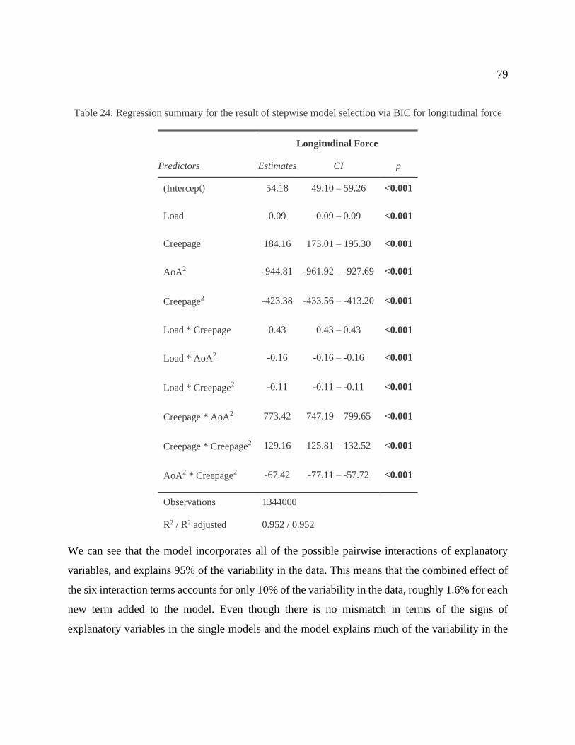
79

Table 24: Regression summary for the result of stepwise model selection via BIC for longitudinal force

Longitudinal Force


(Intercept) 54.18 49.10 – 59.26 <0.001

Load 0.09 0.09 – 0.09 <0.001

Creepage 184.16 173.01 – 195.30 <0.001

AoA2 -944.81 -961.92 – -927.69 <0.001

Creepage2 -423.38 -433.56 – -413.20 <0.001

Load * Creepage 0.43 0.43 – 0.43 <0.001

Load * AoA2 -0.16 -0.16 – -0.16 <0.001

Load * Creepage2 -0.11 -0.11 – -0.11 <0.001

Creepage * AoA2 773.42 747.19 – 799.65 <0.001

Creepage * Creepage2 129.16 125.81 – 132.52 <0.001

AoA2 * Creepage2 -67.42 -77.11 – -57.72 <0.001


R2 / R2 adjusted 0.952 / 0.952

We can see that the model incorporates all of the possible pairwise interactions of explanatory

variables, and explains 95% of the variability in the data. This means that the combined effect of

the six interaction terms accounts for only 10% of the variability in the data, roughly 1.6% for each

new term added to the model. Even though there is no mismatch in terms of the signs of

explanatory variables in the single models and the model explains much of the variability in the

80

data, this model is the most complicated model as far as the pairwise interactions are concerned,

and there probably exists some simpler model that performs as well.

6.3.3 LASSO & Best Subset Selection

In this section, we take the reverse approach and try to eliminate the least important interaction

term from the model from the previous section. Table 25 shows the coefficients estimated by

LASSO for the model, including the main effects and all possible interaction terms except for

𝐶𝑟𝑒𝑒𝑝𝑎𝑔𝑒 ∗ Creepage2.

Table 25: LASSO coefficient estimates for the longitudinal force model including all interactions

Variable Load Creepage AoA2 Creepage2 Load*Creepage Load*AoA2 Load*Creeoage2 Creepage*AoA2 Creepage2*AoA2

Estimate 0.32 0.037 -0.07 -0.061 1.14 -0.21 -0.36 0.00 0.081

We observe that the signs match with these single models and the effect of AoA2 ∗ Creepage2 was

estimated to be zero by the penalized regression model. We combine this result from that of the

best subset selection to determine if the combined results could help us select a simple and

descriptive model. Figure 44 shows the progression of these criteria during the selection process.

Figure 44: Best subset selection criteria for choosing among the longitudinal force models

81

The curves for R2 and AIC flatten out after the fourth step, and this scheme is consistent across the

panels in Figure 44. As mentioned earlier, each point on the curves corresponds to a model during

the progression of the step function. The following are the first four models, respectively:

1. 𝐿𝑜𝑛𝑔𝑖𝑡𝑢𝑑𝑖𝑛𝑎𝑙 𝐹𝑜𝑟𝑐𝑒𝑖 = 𝛽0 + 𝛽1𝑳𝒐𝒂𝒅𝒊 ∗ 𝑪𝒓𝒆𝒆𝒑𝒂𝒈𝒆𝒊 + 𝜀𝑖

2. 𝐿𝑜𝑛𝑔𝑖𝑡𝑢𝑑𝑖𝑛𝑎𝑙 𝐹𝑜𝑟𝑐𝑒𝑖 = 𝛽0 + 𝛽1𝑳𝒐𝒂𝒅𝒊 ∗ 𝑪𝒓𝒆𝒆𝒑𝒂𝒈𝒆𝒊 + 𝛽2𝑳𝒐𝒂𝒅𝒊 ∗ 𝑪𝒓𝒆𝒆𝒑𝒂𝒈𝒆𝟐𝒊

+ 𝜀𝑖

3. 𝐿𝑜𝑛𝑔𝑖𝑡𝑢𝑑𝑖𝑛𝑎𝑙 𝐹𝑜𝑟𝑐𝑒𝑖 = 𝛽0 + 𝛽1𝑳𝒐𝒂𝒅𝒊 + 𝛽2𝑳𝒐𝒂𝒅𝒊 ∗ 𝑪𝒓𝒆𝒆𝒑𝒂𝒈𝒆𝒊 + 𝛽3𝑳𝒐𝒂𝒅𝒊 ∗ 𝑨𝒐𝑨𝟐𝒊 + 𝜀𝑖

4. 𝐿𝑜𝑛𝑔𝑖𝑡𝑢𝑑𝑖𝑛𝑎𝑙 𝐹𝑜𝑟𝑐𝑒𝑖 =

𝛽0 + 𝛽1𝑳𝒐𝒂𝒅𝒊 + 𝛽2𝑳𝒐𝒂𝒅𝒊 ∗ 𝑪𝒓𝒆𝒆𝒑𝒂𝒈𝒆𝒊 + 𝛽3𝑳𝒐𝒂𝒅𝒊 ∗ 𝑨𝒐𝑨𝟐𝒊 + 𝛽4𝑳𝒐𝒂𝒅𝒊 ∗ 𝑪𝒓𝒆𝒆𝒑𝒂𝒈𝒆𝟐

𝒊+ 𝜀𝑖

The selection process starts with the interaction of the wheel load and creepage in the first model,

and then the interactions of wheel load with Creepage2 and R2 are added in the second and third

models. Finally, in the fourth model, the main effect of the wheel load is added to the three

interaction terms. This is consistent with the results of the random forest model and LASSO. We

saw that the wheel load and creepage were the most important variables, with the wheel load far

ahead of creepage. This translated into the first model and the fourth model exhibiting the

prevalence of the effect of the wheel load by incorporating the main effect and all the pairwise

interactions of the wheel load. This makes the fourth model in the subset selection process one of

the strongest candidates for modeling the longitudinal force.

6.3.4 Selected Model

To review, we are left with the main effects of the explanatory variables plus four interaction terms

(Load ∗ AoA2, Load ∗ Creepage, Load ∗ Creepage2, AoA2 ∗ Creepage2) and a maximum effect of

explaining 10 percent of the variability in the data. Different combinations of interaction terms and

the main effects were tested in order to choose the simplest model that explains the data as much

as possible. Many of these models had one of the following issues9:

a) The sign of main effects match with that of the single regression model

b) The coefficient estimates were not significant at a 10% or higher confidence level

9 To avoid redundancy, results are not presented here.

82

c) The model explained no more than the superposition of main effects (R2 < 90%)

These results, in tandem with the previous section, suggest that the following model, which is the

fourth model of the best subset selection, is the simplest and most interpretable model for the

longitudinal force. Table 26 presents the regression summary for the selected model.

𝐿𝑜𝑛𝑔𝑖𝑡𝑢𝑑𝑖𝑛𝑎𝑙 𝐹𝑜𝑟𝑐𝑒𝑖 = 𝛽0 + 𝛽1𝐿𝑜𝑎𝑑𝑖 + 𝛽2𝐿𝑜𝑎𝑑𝑖 ∗ 𝐶𝑟𝑒𝑒𝑝𝑎𝑔𝑒𝑖 + 𝛽3𝐿𝑜𝑎𝑑𝑖 ∗ 𝐴𝑜𝐴2𝑖

+

𝛽4𝐿𝑜𝑎𝑑𝑖 ∗ 𝐶𝑟𝑒𝑒𝑝𝑎𝑔𝑒2𝑖

+ 𝜀𝑖 𝑤ℎ𝑒𝑟𝑒 𝜀𝑖~𝒩(0, 𝕀4𝜎2)

Table 26: Regression summary for the final model of longitudinal force

Longitudinal Force


(Intercept) -132.92 -160.61 – -105.23 <0.001

Load 0.11 0.10 – 0.12 <0.001

Load*Creepage 0.38 0.36 – 0.40 <0.001

Load*AoA2 -0.14 -0.15 – -0.14 <0.001

Load*Creepage2 -0.08 -0.09 – -0.07 <0.001

Observations 1344

R2 / R2 adjusted 0.947 / 0.947

6.4 Distribution of Predictions for Multiple Regression Model

of Longitudinal Force

With the developed model in hand, the only task left is to quantify the uncertainty around the

predictions made by the model. The multiple regression model for the longitudinal force performs

better in terms of meeting the assumptions of the classical linear regression model compared to

the multiple regression model for the lateral force since there were no issues (in terms of meeting

83

the assumptions) with the single models of wheel load and AoA, and the creepage appears only in

the interaction terms. Figure 45 and Figure 46 show the predictions made by the multiple

regression model and the support vector multiple regression model on the testing set versus the

true values, along with the 95% confidence interval of predictions, respectively.

Figure 45: Multiple regression model for longitudinal force, predictions and 95% confidence interval of

predictions

We observe that the predictions of the multiple (parametric) regression model closely follow the

true values (the testing set) and that the 95% confidence interval of predictions is very tight. The

predictions deviate from the true value to a very limited extent when the magnitude of the

longitudinal force is very small or very large. Not all the assumptions of the classical linear

regression model were met by the single models, so we take the same approach as for the lateral

force model and try to compare the results with the distribution of the predictions of an unbiased

(as much as possible) non-parametric model. As mentioned in Section 6.2, we obtain the

distribution of the predictions for the non-parametric model empirically and by bootstrapping over

the residuals.

-

84

Figure 46: SVR model for longitudinal force, predictions and 95% confidence interval of predictions

Figure 46 shows the mean and the 95% prediction interval of the predictions made by a support

vector multiple regression model. The model was trained on the training set and predictions were

made on the testing set. We can see that the predictions almost perfectly follow the true values and

are very tightly distributed around their mean, as was the case with the multiple (parametric)

regression model. In order to compare distributions of the predictions, we only compare the upper

and the lower bounds of the 95% confidence interval of the predictions from both models. The

CDF and density plots of the lower and upper bounds of the 95% confidence interval of predictions

from the multiple (parametric) regression model and the SVR model are presented in Figure 47

and Figure 48, respectively.

-

85

Figure 47: CDF (upper panel) and density plot (lower panel) of the lower bounds of the 95% confidence

interval of predictions from the multiple regression model of longitudinal force and the SVR model

We can see that in both models, the distribution of the upper bounds and the lower bounds of the

confidence intervals are similarly distributed. The Kolmogorov-Smirnov Test results for the

equality of the distributions of the lower bounds and upper bounds of the 95% confidence interval

of the predictions for both models are presented in Table 27 and Table 28, respectively.

Den

sity

Longitudinal Force

86

Figure 48: CDF (upper pane) and density plot (lower pane) of the upper bounds of the 95% confidence

interval of predictions from the multiple regression model of longitudinal force and the SVR model

For both cases, we fail to reject the null hypothesis that the two distributions are statistically

identical at a 1% confidence level. In other words, we can say that the distributions of the upper

bounds and the lower bounds from both models are identically distributed. This piece of evidence

is pretty remarkable since we can argue that the model is accurate enough to serve as a proxy for

Den

sity

Longitudinal Force

87

the true underlying model even though the assumptions of the classical linear regression model do

not completely hold for the parametric regression model.


predictions from the multiple regression model of longitudinal force and the SVR model


D = 0.028993, p-value = 0.01579



predictions from the multiple regression model of longitudinal force and the SVR model


D = 0.025521, p-value = 0.04696


88

7 Conclusions and Recommendations

This chapter summarizes the results presented in the preceding chapters and intends to give a

broader view of the conducted research. This summary is followed by recommendations for

diving deeper into this field and possibilities for future studies.

7.1 Conclusions

From a bird’s eye point of view, this study attempted to bridge the gap between the well-

established analytical models for the wheel-rail contact dynamics and the state-of-the-art

machine/deep learning methods used for parameter estimation and predictions by statistically

modeling the contact dynamics using experimental data. The contribution from this research

becomes more obvious if we take a closer look at the opposite ends of the spectrum.

On one end, we have longitudinal and lateral traction models that take a purely Hertzian

approach, which starts from theory and the assumptions that it entails, and finds its way to

practice via numerical algorithms and software. On the other end of the spectrum, we have

deep neural networks and non-parametric methods that start from experimental data, are not

concerned with the mathematical functional forms in any way, and mostly focus on out-of-

sample performance and the accuracy of predictions in practice. Test rigs play a crucial role

in between and serve both approaches by providing experimental data under controlled

conditions.

The rich data generated by the test rigs, however, remains far from its potential by being treated

as raw input into these two approaches. Statistical models borrow the strengths of both

approaches by letting the data speak for itself. They employ the mathematical functions to

define the relationship among the explanatory variables but make conclusions based on the

performance of the model in practice. Unlike the other two approaches, they provide a margin

for the certainty of predictions in addition to the point estimates. One can see how rich and

practical such models and this new perspective would be.

89

Two groups of statistical models were developed in this research:

1. Single model to study the main effects of AoA, creepage, and wheel load on traction.

2. Multiple models to define the relationship between these variables.

The results presented in Chapter 5 indicate that AoA varies non-linearly with longitudinal and

lateral forces. For the former, the relationship forms a parabolic shape that is modeled by a

quadratic polynomial without a linear term (a single squared term) and perfectly meets all the

assumptions of the classical linear regression model. The cubic polynomial regression model

of lateral forces, however, shows some degree of heteroscedasticity in the residuals.

Creepage shows a linear relationship with the lateral forces but a non-linear relationship with

the longitudinal forces that can be modeled with a quadratic polynomial. As discussed in the

earlier chapters, there is some degree of non-linearity and non-constant variance left in the

residuals of this model, but neither the transformations nor other functional forms could

improve the results.

Wheel load shows a linear relationship with the longitudinal and lateral forces, and the

assumptions of the classical linear regression model are satisfied by these linear models.

All in all, single regression models introduced new dimensions to the features space by

bringing the quadratic terms for AoA and creepage, and a cubic term for AoA, into play.

Comparing the performance of these parametric regression models with their non-parametric

counterparts shows that these models have good predictive power.

On the other hand, multiple regression models show that not all of the newly-introduced

features are significantly influential for the longitudinal and lateral forces when all the

variables are considered.

The multiple regression model for the longitudinal forces pivots on the wheel load and its

interaction with the variables incorporated in the single models of the longitudinal forces. This

makes intuitive sense as it nicely reflects the influence of the wheel load on longitudinal forces

known to railroad researchers. The multiple regression model for the lateral force, however,

indicates that the cubic term for AoA is not necessary in order to make accurate predictions

90

thus its effect is not incorporated into the model. The multiple regression model also accurately

captures the effect of the AoA on lateral forces.

The uncertainties around the predictions by the multiple parametric regression models are very

close and, in the case of longitudinal forces, perfectly match those of the (unbiased) support

vector regression models. This proves that even though not all the assumptions of the classical

linear regression model are met by the single regression models, the prediction intervals and

the uncertainties around the predictions coming from the multiple parametric regression

models are accurate and reliable. This is a significant result and could be considered a step

forward in modeling the contact dynamics from a novel, data-driven perspective. These

models greatly simplify the calculation of traction and are anticipated to be of great use in

practice.

7.2 Recommendations for Future Studies

The statistical models and presented results open up new opportunities for research in this

field. In general, two major lines of research are recommended for future studies:

1. Improving the developed statistical models by:

a. Introducing new variables e.g., investigating the effects of cant angle on the

longitudinal and lateral forces and redefining the multiple regression models,

b. Developing two-stage regression models by defining intermediary variables of

interest and incorporating these new variables in the multiple regression

models,

c. Quantifying the upper and lower bounds for the accuracy of the developed

models,

d. Developing regression models for simultaneous prediction of longitudinal and

lateral forces, and

e. Developing Bayesian models or estimators by incorporating the appropriate

range of explanatory variables as priors.

91

2. Moving towards the state-of-the-art prediction methods tailored for the capabilities of

the VT-FRA Roller Rig by:

i. Developing deep neural networks for predicting:

a. Longitudinal and lateral forces and quantifying the uncertainty

of the predictions by bootstrapping over the final hidden layers,

b. Wheel wear by incorporating the 3D laser scanner data as input,

ii. Developing deep neural networks for predicting multiple responses, and

iii. Developing ensemble methods (multiple learning algorithms) to

maximize predictive performance

Although limited time did not allow for the exploration of these topics, the author hopes that

they will kindle the interest of future researchers at the Center for Vehicle Systems and Safety

and elsewhere.

92

Bibliography

[1] K. S. Baek, K. Kyogoku, and T. Nakahara, “An experimental investigation of transient

traction characteristics in rolling-sliding wheel/rail contacts under dry-wet conditions,”

Wear, vol. 263, no. 1-6 SPEC. ISS., pp. 169–179, 2007, doi: 10.1016/j.wear.2007.01.067.

[2] S. R. Lewis, R. Lewis, and U. Olofsson, “An alternative method for the assessment of

railhead traction,” Wear, vol. 271, no. 1–2, pp. 62–70, 2011, doi:

10.1016/j.wear.2010.10.035.

[3] Y. Zhu, U. Olofsson, and K. Persson, “Investigation of factors influencing wheel-rail

adhesion using a mini-traction machine,” Wear, vol. 292–293, pp. 218–231, 2012, doi:

10.1016/j.wear.2012.05.006.

[4] Q. Guan, J. Zeng, and X. Jin, “An angle of attack-based derailment criterion for wheel

flange climbing,” Proc. Inst. Mech. Eng. Part F J. Rail Rapid Transit, vol. 228, no. 7, pp.

719–729, 2014, doi: 10.1177/0954409713490149.

[5] B. Marquis and R. Greif, “Application of nadal limit in the prediction of wheel climb

derailment,” 2011 Jt. Rail Conf. JRC 2011, pp. 273–280, 2011, doi: 10.1115/JRC2011-

56064.

[6] J. J. O’Shea and A. A. Shabana, “Analytical and numerical investigation of wheel climb at

large angle of attack,” Nonlinear Dyn., vol. 83, no. 1–2, pp. 555–577, 2016, doi:

10.1007/s11071-015-2347-z.

[7] S. Iwnicki, M. Spiryagin, C. Cole, and T. McSweeney, Eds., Handbook of Railway Vehicle

Dynamics, Second. Taylor & Francis, 2006.

[8] S. Z. Meymand, A. Keylin, and M. Ahmadian, “A survey of wheel-rail contact models for

rail vehicles,” Veh. Syst. Dyn., vol. 54, no. 3, pp. 386–428, 2016, doi:

10.1080/00423114.2015.1137956.

[9] E. A. H. Vollebregt, “Numerical modeling of measured railway creep versus creep-force

curves with CONTACT,” Wear, vol. 314, no. 1–2, pp. 87–95, 2014, doi:

10.1016/j.wear.2013.11.030.

[10] O. Polach, “Creep forces in simulations of traction vehicles running on adhesion limit,”

Wear, vol. 258, no. 7–8, pp. 992–1000, 2005, doi: 10.1016/j.wear.2004.03.046.

[11] J. J. Kalker and K. L. Johnson, “Three-Dimensional Elastic Bodies in Rolling Contact,” J.

93

Appl. Mech., vol. 60, no. 1, pp. 255–255, 1993, doi: 10.1115/1.2900773.

[12] M. Spiryagin, O. Polach, and C. Cole, “Creep force modelling for rail traction vehicles

based on the Fastsim algorithm,” Veh. Syst. Dyn., vol. 51, no. 11, pp. 1765–1783, 2013, doi:

10.1080/00423114.2013.826370.

[13] J. Santamaria, E. G. Vadillo, and J. Gomez, “Influence of creep forces on the risk of

derailment of railway vehicles,” Veh. Syst. Dyn., vol. 47, no. 6, pp. 721–752, 2009, doi:

10.1080/00423110802368817.

[14] X. Jin, P. Wu, and Z. Wen, “Effects of structure elastic deformations of wheelset and track

on creep forces of wheel/rail in rolling contact,” Wear, vol. 253, no. 1–2, pp. 247–256, 2002,

doi: 10.1016/S0043-1648(02)00108-4.

[15] A. Alonso, A. Guiral, L. Baeza, and S. Iwnicki, “Wheel-rail contact: Experimental study of

the creep forces-creepage relationships,” Veh. Syst. Dyn., vol. 52, no. SUPPL. 1, pp. 469–

487, 2014, doi: 10.1080/00423114.2014.907923.

[16] M. Hosseinipour, “Electromechanical Design and Development of the Virginia Tech Roller

Rig Testing Facility for Wheel-Rail Contact Mechanics and Dynamics,” 2016.

[17] K. Matsudaira, T., Matsui, N., Arai, S., and Yokose, “Problems on Hunting of Railway

Vehicle on Test Stand,” ASME J. Eng. Ind., 91, pp. 879–885, 1969.

[18] R. V. Dukkipati, “Lateral stability analysis of a railway truck on roller rig,” Mech. Mach.

Theory, vol. 36, no. 2, pp. 189–204, 2001, doi: 10.1016/S0094-114X(00)00017-3.

[19] R. V. Dukkipati, “Lateral stability simulation of a rail truck on roller rig,” JSME

International Journal, Series C: Mechanical Systems, Machine Elements and

Manufacturing, vol. 45, no. 1. pp. 168–175, 2002, doi: 10.1299/jsmec.45.168.

[20] R. V. Dukkipati, “Modelling and simulation of the hunting of a three-piece railway truck

on NRC curved track simulator,” Veh. Syst. Dyn., vol. 23, no. sup1, pp. 105–115, 1994, doi:

10.1080/00423119308969508.

[21] R. Stock, D. T. Eadie, D. Elvidge, and K. Oldknow, “Influencing rolling contact fatigue

through top of rail friction modifier application - A full scale wheel-rail test rig study,”

Wear, vol. 271, no. 1–2, pp. 134–142, 2011, doi: 10.1016/j.wear.2010.10.006.

[22] A. Jaschinski, H. Chollet, S. Iwnicki, A. Wickens, and J. Von Würzen, “The application of

roller rigs to railway vehicle dynamics,” Veh. Syst. Dyn., vol. 31, no. 5–6, pp. 345–392,

1999, doi: 10.1076/vesd.31.5.345.8360.

[23] Wheel-Rail Interface Handbook. Elsevier, 2009.

[24] H. Chollet, “Etude en similitude mécanique des efforts tangents au contact roue-rail,” 1991.

94

[25] M. Jochim, “Analyse der Dynamik eines Schienenfahrzeuges,” 1987.

[26] S. Iwnicki and Z. Shen, “Collaborative railway roller rig project,” in SEFI World Conf. Eng.

Educ., Portsmouth, 1992.

[27] S. D. Iwnicki and A. H. Wickens, “Validation of a MATLAB railway vehicle simulation

using a scale roller rig,” Veh. Syst. Dyn., vol. 30, no. 3–4, pp. 257–270, 1998, doi:

10.1080/00423119808969451.

[28] M. Gretzschel and A. Jaschinski, “Design of an active wheelset on a scaled roller rig,” Veh.

Syst. Dyn., vol. 41, no. 5, pp. 365–381, 2004, doi: 10.1080/00423110412331300336.

[29] J. Kalivoda and P. Bauer, “Roller Rig Implementation of Active Wheelset Steering,” in

Proceedings of the First International Conference on Railway, 2012.

[30] J. Kalivoda and P. Bauer, “Scaled roller rig experiments with a mechatronic bogie,” in

Proceedings of the Second International Conference on Railway, 2014.

[31] A. Rovira, A. Roda, R. Lewis, and M. B. Marshall, “Application of Fastsim with variable

coefficient of friction using twin disc experimental measurements,” Wear, vol. 274–275,

pp. 109–126, 2012, doi: 10.1016/j.wear.2011.08.019.

[32] A. Rovira, A. Roda, M. B. Marshall, H. Brunskill, and R. Lewis, “Experimental and

numerical modelling of wheel-rail contact and wear,” Wear, vol. 271, no. 5–6, pp. 911–924,

2011, doi: 10.1016/j.wear.2011.03.024.

[33] N. Bosso, A. Gugliotta, and A. Somà, “Dynamic identification of a 1:5 scaled railway bogie

on roller rig,” in WIT Transactions on the Built Environment, 2006, vol. 88, pp. 829–838,

doi: 10.2495/CR060811.

[34] N. Bosso and N. Zampieri, “Real-time implementation of a traction control algorithm on a

scaled roller rig,” Veh. Syst. Dyn., vol. 51, no. 4, pp. 517–541, Apr. 2013, doi:

10.1080/00423114.2012.750001.

[35] N. Bosso and N. Zampieri, “Experimental and Numerical Simulation of Wheel-Rail

Adhesion and Wear Using a Scaled Roller Rig and a Real-Time Contact Code,” Shock Vib.,

vol. 2014, pp. 1–14, 2014, doi: 10.1155/2014/385018.

[36] A. Matsumoto et al., “Creep force characteristics between rail and wheel on scaled model,”

Wear, vol. 253, no. 1–2, pp. 199–203, Jul. 2002, doi: 10.1016/S0043-1648(02)00100-X.

[37] A. Matsumoto, Y. Sato, H. Ono, M. Tanimoto, Y. Oka, and E. Miyauchi, “Formation

mechanism and countermeasures of rail corrugation on curved track,” Wear, vol. 253, no.

1–2, pp. 178–184, Jul. 2002, doi: 10.1016/S0043-1648(02)00097-2.

[38] Q. Y. Liu, B. Zhang, and Z. R. Zhou, “An experimental study of rail corrugation,” Wear,

95

vol. 255, no. 7–12, pp. 1121–1126, Aug. 2003, doi: 10.1016/S0043-1648(03)00213-8.

[39] E. Meli and A. Ridolfi, “An innovative wheel–rail contact model for railway vehicles under

degraded adhesion conditions,” Multibody Syst. Dyn., vol. 33, no. 3, pp. 285–313, Dec.

2013, doi: 10.1007/s11044-013-9405-4.

[40] B. Allotta, E. Meli, A. Ridolfi, and A. Rindi, “Development of an innovative wheel–rail

contact model for the analysis of degraded adhesion in railway systems,” Tribol. Int., vol.

69, pp. 128–140, Jan. 2014, doi: 10.1016/j.triboint.2013.09.013.

[41] B.-G. Eom, B.-B. Kang, and H.-S. Lee, “A Running Stability Test of 1/5 Scaled Bogie using

Small-Scaled Derailment Simulator,” J. Korean Soc. Railw., vol. 15, no. 1, pp. 9–16, Feb.

2012, doi: 10.7782/JKSR.2012.15.1.009.

[42] B.-G. Eom, B.-B. Kang, and H. S. Lee, “A study on running stability assessment methods

for 1/5 small scaled bogie of saemaul using small-scaled derailment simulator,” Int. J.

Precis. Eng. Manuf., vol. 14, no. 4, pp. 589–598, Apr. 2013, doi: 10.1007/s12541-013-0079-

x.

[43] S. Z. Meymand, M. J. Craft, and M. Ahmadian, “On the application of roller rigs for

studying rail vehicle systems,” in American Society of Mechanical Engineers, Rail

Transportation Division (Publication) RTD, 2013, pp. 1–10, doi: 10.1115/rtdf2013-4724.

[44] A. Radmehr, A. Tajaddini, B. Marquis, and M. Ahmadian, “Virginia Tech-Federal Railroad

Administration Roller Rig Measurement Capabilities and Baseline Measurements,” in

Proceedings of the 2019 ASME Joint Rail Conference JRC2019.

[45] A. Shebani and S. Iwnicki, “Prediction of wheel and rail wear under different contact

conditions using artificial neural networks,” Wear, vol. 406–407, no. March 2017, pp. 173–

184, 2018, doi: 10.1016/j.wear.2018.01.007.

[46] K. Nachtigall and S. Voget, “A genetic algorithm approach to periodic railway

synchronization,” Comput. Oper. Res., vol. 23, no. 5, pp. 453–463, 1996, doi:

10.1016/0305-0548(95)00032-1.

[47] H. Parkinson and S. Iwnicki, “An Intelligent Track Monitoring System.”

[48] I. Persson and S. D. Iwnicki, “Optimisation of railway wheel profiles using a genetic

algorithm,” Veh. Syst. Dyn., vol. 41, no. SUPPL., pp. 517–526, 2004.

[49] G. James, D. Witten, T. Hastie, and R. Tibshirani, An Introduction to Statistical Learning

with Applications in R. 2019.

[50] “Coefficient of determination - Wikipedia.” [Online]. Available:

https://en.wikipedia.org/wiki/Coefficient_of_determination.

96

[51] S. Fisher Ellison, “Data Analysis for Social Scientists Course Notes, Department of

Economics at MIT.” Boston, MA, 2019.

[52] R. B. Gramacy, “Data Analytics I Course Notes, Department of Statistics at Virginia Tech.”

Blacksburg, VA, 2019.

[53] M. B. Wilk and R. Gnanadesikan, “Probability plotting methods for the analysis of data.,”

Biometrika, vol. 55, no. 1, pp. 1–17, 1968, doi: 10.1093/biomet/55.1.1.

[54] “Q–Q plot - Wikipedia.” [Online]. Available: https://en.wikipedia.org/wiki/Q–Q_plot.

[55] T. Hastie, R. Tibshirani, and J. Friedman, The Elements of Statistical Learning: Data

Mining, Inference, and Prediction, Second Edition. 2017.

[56] H. Hotelling, “Relations Between Two Sets of Variates,” Biometrika, vol. 28, no. 3, pp.

321–377, 1936.

[57] “Principal component analysis - Wikipedia.” [Online]. Available:

https://en.wikipedia.org/wiki/Principal_component_analysis.

[58] “Kernel Methods for Regression: Support Vector Regression, Gaussian Mixture

Regression, Gaussian Process (EPFL Machine Learning, Course Notes).” EPFL.

[59] “Kolmogorov–Smirnov test - Wikipedia.” [Online]. Available:

https://en.wikipedia.org/wiki/Kolmogorov–Smirnov_test.

[60] A. Radmehr, K. Kothari, and M. Ahmadian, “Evaluating the Effect of Natural Third Body

Layers on Friction Using the Virginia Tech Roller Rig,” Proc. 2019 ASME Jt. Rail Conf.

JRC2019 April 10-12, 2019, Snowbird, UT, USA, 2019.

[61] R-Core-Team, “R: A language and environment for statistical computing.” R Foundation

for Statistical Computing, Vienna, Austria, 2020.

A Statistical Approach to Modeling Wheel-Rail Contact Dynamics

Documents

Transcript of A Statistical Approach to Modeling Wheel-Rail Contact Dynamics