A Stable Algorithm for Non-Negative Invariant

Numerical Solution of Reaction-Diffusion Systems on

Complicated Domains

Insoon Yang

Electrical Engineering and Computer SciencesUniversity of California at Berkeley

Technical Report No. UCB/EECS-2012-77

http://www.eecs.berkeley.edu/Pubs/TechRpts/2012/EECS-2012-77.html

May 10, 2012

Copyright © 2012, by the author(s).All rights reserved.

Permission to make digital or hard copies of all or part of this work forpersonal or classroom use is granted without fee provided that copies arenot made or distributed for profit or commercial advantage and that copiesbear this notice and the full citation on the first page. To copy otherwise, torepublish, to post on servers or to redistribute to lists, requires prior specificpermission.

Acknowledgement

First of all, I owe my deepest gratitude to my advisor, Professor ClaireTomlin, who has extended her valuable support and encouragementthroughout this work. I thank her for inspiring me during our discussions totake various perspectives on my work.I am also thankful to Professors Phillip Colella and L. Craig Evans. I willnever forget Prof. Colella’s advice that a good algorithm for numericalsolution of a partial differential equation (PDE) should be based on a solidunderstanding of its analytic solution. Prof. Evans provided wonderful PDEcourses, in which I learned modern PDE theory. I also appreciate hiswillingness to answer my questions on reaction-diffusion systems.

A Stable Algorithm for Non-Negative Invariant Numerical Solution ofReaction-Diffusion Systems on Complicated Domains

by

Insoon Yang

B.S. (Seoul National University) 2009

A thesis submitted in partial satisfactionof the requirements for the degree of

Master of Science

in

Engineering - Electrical Engineering and Computer Sciences

in the

GRADUATE DIVISION

of the

UNIVERSITY OF CALIFORNIA, BERKELEY

Committee in charge:

Professor Claire J. Tomlin, ChairProfessor Phillip Colella

Spring 2012

The thesis of Insoon Yang is approved.

Chair Date

Date

University of California, Berkeley

Spring 2012

A Stable Algorithm for Non-Negative Invariant Numerical Solution of

Reaction-Diffusion Systems on Complicated Domains

Copyright c© 2012

by

Insoon Yang

Abstract

A Stable Algorithm for Non-Negative Invariant Numerical Solution of

Reaction-Diffusion Systems on Complicated Domains

by

Insoon Yang

Master of Science in Engineering - Electrical Engineering and Computer Sciences

University of California, Berkeley

Professor Claire J. Tomlin, Chair

We present a Cartesian grid finite difference numerical method for solving a system of

reaction-diffusion initial boundary value problems with Neumann type boundary conditions.

The method utilizes adaptive time-stepping, which guarantees stability and non-negativity

of the solutions. The latter property is critical for models in biology where solutions rep-

resent physical measurements such as concentration. The level set representation of the

boundary enables us to handle domains with complicated geometry with ease. We pro-

vide numerical validation of our method on synthetic and biological examples. Empirical

tests demonstrate second order convergence rate in the L1- and L2-norms, as well as in the

L∞-norm for many cases.

Professor Claire J. TomlinThesis Committee Chair

1

Contents

Contents i

List of Figures iii

List of Tables iv

Acknowledgements v

1 Introduction 1

1.1 Related work . . . . . . . . . . . . . . . . . . . . . . . . . . . . . . . . . . . 3

1.2 Outline of the thesis . . . . . . . . . . . . . . . . . . . . . . . . . . . . . . . 4

2 Spatial discretization 6

2.1 Notation and setup . . . . . . . . . . . . . . . . . . . . . . . . . . . . . . . . 6

2.2 Regular and Irregular grid points . . . . . . . . . . . . . . . . . . . . . . . . 7

2.3 Computing the outward normal directions . . . . . . . . . . . . . . . . . . . 9

2.4 Extending the normal line into Ω . . . . . . . . . . . . . . . . . . . . . . . . 11

2.5 Approximating u on the extension points . . . . . . . . . . . . . . . . . . . 13

2.6 Approximating u on the boundary . . . . . . . . . . . . . . . . . . . . . . . 14

3 Non-negative invariance and stability 16

3.1 Temporal discretization . . . . . . . . . . . . . . . . . . . . . . . . . . . . . 16

3.2 Non-negative invariance . . . . . . . . . . . . . . . . . . . . . . . . . . . . . 17

3.3 Stability . . . . . . . . . . . . . . . . . . . . . . . . . . . . . . . . . . . . . . 18

4 Complete algorithm and convergence rate analysis 21

4.1 Convergence rate analysis . . . . . . . . . . . . . . . . . . . . . . . . . . . . 23

i

5 Numerical results 24

5.1 Convergence test on a circular domain . . . . . . . . . . . . . . . . . . . . . 24

5.2 Convergence test on an annulus . . . . . . . . . . . . . . . . . . . . . . . . . 27

5.3 Convergence test of a two-species system . . . . . . . . . . . . . . . . . . . . 28

5.4 A multi-species system in a star-shaped cell . . . . . . . . . . . . . . . . . . 30

5.5 EphA2/Ephrin-A1 signaling . . . . . . . . . . . . . . . . . . . . . . . . . . . 33

6 Conclusion 37

Bibliography 38

References . . . . . . . . . . . . . . . . . . . . . . . . . . . . . . . . . . . . . . . . 38

ii

List of Figures

2.1 (i, j) is an irregular point whose right and bottom arms are intersected by the boundary

of the domain. . . . . . . . . . . . . . . . . . . . . . . . . . . . . . . . . . . . 8

2.2 The rule for choosing N xy or N y

x for approximating the slope of normal vector: if the

boundary intersects a horizontal grid line we approximate φx/φy by N xy (Circles); if the

boundary intersects a vertical grid line we approximate φy/φx by N yx (Triangles). . . . 10

2.3 Normal lines extended inwardly (blue) and their intersections (extension points) with inner

and outer boxes of the boundary point of interest, R. . . . . . . . . . . . . . . . . . 12

2.4 Normal lines extended inwardly (blue) and their intersections (extension points) with inner

and outer boxes of the boundary point of interest, B. . . . . . . . . . . . . . . . . . 12

2.5 Approximation of the solution at the boundary point R interpolating the extension points P

and Q. Note that, for approximating uP , we consider the four square points and eventually

use (i, j), (i, j + 1) and (i, j + 2) for the approximation because (i, j − 1) is outside of the

domain. To approximate uQ, we first detect the four diamond points and then utilize

(i− 1, j), (i− 1, j + 1) and (i− 1, j + 2) for the approximation since the distance between

(i− 1, j) and Q is shorter than the distance between (i− 1, j + 3) and Q. . . . . . . . 13

5.1 The solution u1 at T = 1 on a 100× 100 grid. . . . . . . . . . . . . . . . . . . . . 25

5.2 The absolute error |u1 − uA1 | at T = 0.01 on a 100× 100 grid. . . . . . . . . . . . . . 26

5.3 The solution u1 on a 100× 100 grid. . . . . . . . . . . . . . . . . . . . . . . . . . 27

5.4 The numerical solution of u1 on a 100× 100 grid. . . . . . . . . . . . . . . . . . . . 31

5.5 The numerical solution of u2 on a 100× 100 grid. . . . . . . . . . . . . . . . . . . . 31

5.6 The numerical solution of u3 on a 100× 100 grid. . . . . . . . . . . . . . . . . . . . 32

5.7 An EphA2/Ephrin-A1 downstream signaling mechanism and the crosstalk between RhoA,

Rac1 and Cdc42. . . . . . . . . . . . . . . . . . . . . . . . . . . . . . . . . . . 33

5.8 The first column shows the experimental data of Ephrin-A1 (courtesy of Jay T. Groves).

The second and third columns are numerical solutions of pRac1 and pCdc42, respectively

on a 200 × 200 grid. Rows represent the results at T = 2.5, T = 5, T = 7.5 and T = 10

from top to bottom. . . . . . . . . . . . . . . . . . . . . . . . . . . . . . . . . . 36

iii

List of Tables

5.1 Errors and convergence rates of the example simulated in a circular domainfor T = 1. . . . . . . . . . . . . . . . . . . . . . . . . . . . . . . . . . . . . 25

5.2 Errors and convergence rates of the example simulated in a circular domainfor T = 0.01. . . . . . . . . . . . . . . . . . . . . . . . . . . . . . . . . . . . 26

5.3 Errors and convergence rates of the example simulated in a circular domainwith a hole. . . . . . . . . . . . . . . . . . . . . . . . . . . . . . . . . . . . 28

5.4 Errors and convergence rates of the example with multiple species simulatedin a circular domain, when D = (0.1, 0.05). . . . . . . . . . . . . . . . . . . 29

5.5 Errors and convergence rates of the example with multiple species simulatedin a circular domain, when D = (0.1, 0.001). . . . . . . . . . . . . . . . . . 29

5.6 Errors and convergence rates of the example simulated in a star-shaped do-main. . . . . . . . . . . . . . . . . . . . . . . . . . . . . . . . . . . . . . . . 32

iv

Acknowledgements

First of all, I owe my deepest gratitude to my advisor, Professor Claire Tomlin, who has

extended her valuable support and encouragement throughout this work. I thank her for

inspiring me during our discussions to take various perspectives on my work.

I am also thankful to Professors Phillip Colella and L. Craig Evans. I will never forget

Prof. Colella’s advice that a good algorithm for numerical solution of a partial differential

equation (PDE) should be based on a solid understanding of its analytic solution. Prof.

Evans provided wonderful PDE courses, in which I learned modern PDE theory. I also

appreciate his willingness to answer my questions on reaction-diffusion systems.

Finally, I would like to thank Professors Ronald Fedkiw, Frederic Gibou, Stanley Osher

and Richard Tsai for feedback on previous versions of the thesis, and Professor Jay Groves

and his lab for providing image data of Ephrin-A1 intracellular distribution.

v

vi

Chapter 1

Introduction

Consider the following reaction-diffusion system for a vector valued function u =

(u1, u2, . . . , uM ) with Neumann boundary conditions:

∂um∂t

= Dm∆um + fm(x, y, t, u) in Ω× (0, T ) (1.1a)

∂um∂ν

= 0 on ∂Ω× (0, T ) (1.1b)

um(x, 0) = u0m(x) on Ω× t = 0, (1.1c)

for m = 1, · · · ,M . The domain Ω is an open, bounded and connected subset of R2, whose

boundary is ∂Ω. The vector ν denotes the outward unit normal vector to the domain andDm

denotes the diffusion rate for each m = 1, · · · ,M . Similar to u, we write u0 := (u01, · · · , u0M ),

f := (f1, · · · , fM ). Here we assume that f is continuously differentiable. The system (1.1)

has been widely used as a fundamental model for describing biological pattern formation

[17], [42], spatio-temporal biological signaling [1], [15], population dynamics [5], [26] and

chemical reactions [16], [18]. Although we shall mainly focus on the Neumann boundary

conditions (1.1b), the method presented in this thesis is also applicable to general Robin

boundary conditions.

While the structure of reaction-diffusion system (1.1) is quite similar to the heat equa-

tion, their behaviors are generally very different due to the nonlinear forcing term f . For

example, blowing up in L∞ in a finite time occurs for some f , i.e, the solution u of the reac-

1

tion diffusion system (1.1) when f are not in L∞(Ω× [0, T ]) [32]. In addition, the solution

to reaction-diffusion systems often represents physical, chemical, and biological components

such as the concentration level of chemicals and morphogens, which are non-negative by

definition. Thus, analytical conditions for non-negative invariance of the solution is crucial

in modeling these applications. To guarantee the global existence and the non-negative in-

variance of the classical solution we apply the result of invariant sets of the reaction-diffusion

systems [20]–[22] to [0,+∞)M : assume for all m = 1, · · · ,M , and for all (x, t) ∈ Ω× (0, T ),

(A1) fm(x, t, u1, · · · , um−1, 0, um+1, · · · , uM ) ≥ 0 for each u ∈ [0,+∞)M , and

(A2) there exist constants c and d, such that fm(x, t, u) ≤ cum + d for each u ∈ [0,+∞)M .

Condition (A1) is called the quasi-positivity of f , which ensures that [0,+∞)M is an invari-

ant set of the reaction-diffusion system [20]. Condition (A2) uniformly bounds fm by an

affine function of um to prevent the solution from blowing-up in finite time. Note that the

conditions are more strict than the conditions given in [31] for global existence of a classical

solution to reaction-diffusion systems.

In this thesis, we develop a novel algorithm for solving (1.1) that numerically realizes

the constraints (A1) and (A2). We employ a level set representation of ∂Ω; Neumann

boundary conditions are enforced at the boundaries using the normal direction extracted

from the level set representation. While level set representation of the domain boundary

has been used prior to our work, the extraction of the outward normal directions using a

third order accurate gradient of the level set function is novel. The main advantages of our

approach are:

1. The scheme is provably stable and guarantees the solution to be non-negative invari-

ant.

2. The level set representation allows us to handle arbitrarily complicated domain ge-

ometry and the Neumann boundary condition with ease.

3. The method is provably second order in the L1-norm.

2

The importance of stability is clear. Furthermore, the non-negative invariance is necessary

in modeling a physical phenomena, such as chemical concentration, in a meaningful way.

The ease of handling arbitrarily complicated domains is useful, for example, when modeling

the temporal evolution of the distribution of chemical species in a biological cell. Also,

the robustness of the level set method to moving interfaces or sets may complement our

approach to problems of solving (1.1) in moving domains. While we can prove a second order

convergence in the L1-norm, empirical tests have demonstrated a second order convergence

in many cases in L2-norm and the L∞-norm.

1.1 Related work

Numerical methods for solving reaction-diffusion systems on irregular domains have

been developed in the context of the heat equation and the reaction-diffusion equation. We

list several related methods below:

• The finite element method using unstructured meshes has been widely used for solving

partial differential equations in a domain with complex geometry [14]. However, the

mesh generation over an irregular domain is often a complicated process and compu-

tationally expensive, which makes the implementation of the finite element method

not as simple as those of the finite difference and finite volume methods utilizing

Cartesian grids.

• The immersed interface method [19] was originally developed for solving the elliptic

equations with coefficients and forcing terms that are discontinuous across the inter-

face on Cartesian grids. It uses a local coordinate transformation, which results in

a system of linear equations to approximate the solution value at a point near the

boundary. Although the original version of the algorithm requires appropriate jump

conditions on the solution and its normal derivative, which are not generally available

in practice, it has been modified in [6] to solve the heat equations with the Neumann

boundary condition without requiring the jump conditions. However, the six-point

3

stencil selecting method in [6] near the interface is not trivial, and furthermore, it is

not clear that the modified method has a consistent convergence rate.

• The ghost fluid method [4] is applicable to solving parabolic equations with second-

order and fourth-order accuracy [7], [8]. Its advantage is its simplicity of handling

irregular domains by construction of a ghost solution on each side of the interface,

which is easily generalized in the three dimensional case. However, it requires jump

conditions at the boundary to utilize the information from the both sides of the

interface.

• The conceptual idea suggested by Morton and Myers using interpolation along the

normal is similar to the way we handle the domain with complex geometry, but it lacks

of the discussion of stability and the detailed methods for computing normals [25].

• The Cartesian grid embedded boundary methods (or the cut-cell methods) are finite

volume methods for approximating fluxes between volumes using interpolation; it

naturally resolves the problem of mesh generation of irregular domains [13], [23],

[40]. This method is also extended to the three-dimensional and surface diffusion

problems [35], [36]. An important variant of the cut-cell type method is [29], which

yields a symmetric discretization when a domain is divided by an interface. These

methods are implicit, which suggest good stability properties; however, no proof has

been shown for stability.

• The moving boundary node method is another finite volume method that projects the

grid points near the boundary onto the boundary. This method is easily applicable

to the three dimensional case [43]. However, as with the previous work, no proof has

been shown for stability.

1.2 Outline of the thesis

In Section 2, we propose a novel spatial discretization method for the Laplacian or

diffusion operator on a domain with complex geometry. Then in Section 3 we discuss

4

conditions on time steps for guaranteeing the non-negative invariance of the solution and

the stability. We also prove that the adaptive time stepping is uniformly-bounded from

below, followed by proposing a complete algorithm in Section 4. Numerical tests for the

convergence rate of the method are examined and verified with examples in Sections 4.1

and 5, respectively.

5

Chapter 2

Spatial discretization

2.1 Notation and setup

Without loss of generality we can assume that Ω is contained in a rectangular region

[xmin, xmax] × [ymin, ymax] since Ω is bounded. Let us discretize the box into a uniform

Cartesian grid of size N ×N so that xi = xmin + (i − 1) · h and yi = ymin + (i − 1) · h for

i = 1, · · · , N . Here h = (N − 1)/(xmax − xmin) = (N − 1)/(ymax − ymin) is the grid spacing

in the x and y directions. We denote by unm,i,j the numerical approximation of um(xi, yj , tn)

for each m = 1, · · · ,M .

Let φ : R2 → R be a signed-distance (level set) function, whose zero sub-level set

corresponds to Ω:

φ(x, y) =

dist

((x, y),Ω

)if (x, y) ∈ Ωc,

−dist((x, y),Ωc

)if (x, y) ∈ Ω,

(2.1)

where dist(·, ·) is the geodesic distance between two sets in R2. In this thesis, we assume an

exact φ is given for the pre-defined domain Ω. In practice, for arbitrarily shaped Ω, highly

accurate numerical techniques for constructing signed-distance functions are available [2],

[41].

6

2.2 Regular and Irregular grid points

Our first goal is approximating ∆u = uxx + uyy on the right hand side of (1.1a). For

notational convenience we suppress the vector index m and the time index n, in unm,i,j and

um. We begin by categorizing the grid points inside the domain as follows: a grid point

is called regular if its four neighboring grid points are inside the domain; otherwise, it is

called irregular. For a regular grid point at the location (i, j) we use the standard five point

stencil finite difference scheme for approximating the operator:

∆u(xi, xj , tn) ≈ ui+1,j − 2ui,j + ui−1,jh2

+ui,j+1 − 2ui,j + ui,j−1

h2. (2.2)

We discretize (1.1) in time using the forward Euler scheme in which case the local truncation

error is second-order in space. If (i, j) is irregular, however, the standard finite difference

method is not applicable since at least one of ui−1,j , ui+1,j , ui,j−1 and ui,j+1 is not defined.

We further assume that at least one of (i − 1, j) and (i + 1, j) lies inside the domain, and

at least one of (i, j − 1) and (i, j + 1) lies inside the domain. Without loss of generality, we

suppose that (i− 1, j) and (i, j + 1) are inside the domain, and (i+ 1, j) and (i, j − 1) are

outside the domain. We note the case in which only one neighboring point is outside the

domain is naturally included. As shown in Figure 2.1, the right and bottom arms of (i, j)

have intersections with the boundary. Let us refer to these intersection points as R and B

with coordinates (i + ai+1,j , j) and (i, j − ai,j−1), respectively, where ai+1,j , ai,j−1 ∈ [0, 1).

In addition, we let UR and UB denote the analytic solutions at R and B. If we have a third

order accurate approximation uR and uB of UR and UB, respectively, the following scheme

with the forward Euler time integration has the first-order local truncation error in space:

∆u(xi, xj , tn) ≈(uR − ui,jai+1,jh

− ui,j − ui−1,jh

)2

(ai+1,j + 1)h

+

(ui,j+1 − ui,j

h− ui,j − uB

ai,j−1h

)2

(ai,j−1 + 1)h.

(2.3)

Definition 1. Denote ∆hui,j as the discretization (2.2) if (i, j) is a regular point and (2.3)

if (i, j) is a irregular point.

Our first main contribution is a method for obtaining third order accurate approxima-

7

(i, j)

(i, j + 1)

(i 1, j)

B

R

ai+1,jh

ai,j1h

Figure 2.1. (i, j) is an irregular point whose right and bottom arms are intersected by the boundary of

the domain.

tions of the solution at the boundary points UR and UB with Neumann boundary conditions.

We outline the procedure below:

Step 1: Compute the outward normal directions, i.e. slope of ν, on the boundary points

with third-order accuracy. This is achieved by computing a third order approximation

of the gradient of the level set function φ.

Step 2: Extend the normal inward to the domain and choose two points that intersect

the grid lines.

Step 3: Approximate the solution at these intersecting points using the second-order

interpolation of three neighboring points.

Step 4: Approximate the solution at the boundary points R and B by extrapolating

the two solution values with the information of the normal derivative at the boundary.

Now we examine each step in detail and justify the third-order accuracy.

Remark 2. We note that problems with Dirichlet boundary conditions can also be handled

by our method because the values of uR and uB are given as boundary conditions. Therefore

8

we can handle the problems with Robin boundary conditions, p∂u/∂ν + qu = b, without

significant additional effort.

2.3 Computing the outward normal directions

Approximation of φx and φy at (i, j) with third-order accuracy is achieved by

φx(xi, yj) ≈1

3

(2φi+1,j − φi−1,j

h− φi+2,j − φi−2,j

4h

)=: φnumx,i,j , (2.4)

φy(xi, yj) ≈1

3

(2φi,j+1 − φi,j−1

h− φi,j+2 − φi,j−2

4h

)=: φnumy,i,j . (2.5)

Furthermore, we show that the discretizations (2.4) and (2.5) are sufficient to approximate

the slopes φx/φy or φy/φx to third order accuracy.

Proposition 2.3.1. Suppose that φnumx,i,j and φnumy,i,j are defined as in (2.4) and (2.5). Then

we have the following estimates:

φx(xi, yj)

φy(xi, yj)−φnumx,i,j

φnumy,i,j

= O(h3), if φy 6= 0, (2.6)

φy(xi, yj)

φx(xi, yj)−φnumyi,j

φnumx,i,j

= O(h3), if φx 6= 0. (2.7)

Proof. We shall only prove (2.6); (2.7) follows via a similar argument. First, suppress i, j,

xi, yj in the expression for notational convenience, and note that

φnumx

φnumy

=φx +O(h3)

φy +O(h3)

=φxφy

+(φy − φx)

(φy +O(h3))φyO(h3).

Note that (φy −φx)/((φy +O(h3))φy) is bounded by a constant as h→ 0 since φy 6= 0.

Interpolating this approximation of slopes at grid points near the boundary, we now ap-

proximate the slopes at the points on the boundary with third-order accuracy. Note that,

points on the boundary with very large absolute value of curvature would have abrupt

changes in the numerical values of the slopes. Therefore, the interpolation should be

9

(i, j)

(i, j + 1)

(i 1, j)

B

RN x

y (ai+1,j)

N yx (ai,j1)

Figure 2.2. The rule for choosing N xy or N y

x for approximating the slope of normal vector: if the boundary

intersects a horizontal grid line we approximate φx/φy by N xy (Circles); if the boundary intersects a vertical

grid line we approximate φy/φx by N yx (Triangles).

designed to robustly treat the possibility of a numerical discontinuity. Essentially non-

oscillatory (ENO) interpolation [38], [39] is well-suited for interpolating such functions.

In particular, to approximate the slope with third-order accuracy, it suffices to use the

second-order ENO interpolation.

Recall R, the point (i+ ai+1,j , j) between (i, j) and (i+ 1, j) where the horizontal grid

line y = yj intersects the boundary of Ω. Let φx,R be the exact value of φx at R, and

similarly for φy,R. We approximate the slope of the gradient φx,R/φy,R by a quadratic ENO

polynomial

φx,Rφy,R

≈ φx,i,jφy,i,j

+

(φx,i+1,j

φy,i+1,j− φx,i,jφy,i,j

)ai+1,j +Hxai+1,j(ai+1,j − 1)h2

=: N xy (ai+1,j),

(2.8)

which is third order accurate. Here, Hx is chosen as the coefficient corresponding to less

oscillatory polynomial interpolation, i.e., let

Hx =

H+x if |H+

x | < |H−x |,

H−x otherwise,

10

where

H+x =

1

2h2

(φx,i+2,j

φy,i+2,j− 2

φx,i+1,j

φy,i+1,j+φx,i,jφy,i,j

),

H−x =1

2h2

(φx,i+1,j

φy,i+1,j− 2

φx,i,jφy,i,j

+φx,i−1,jφy,i−1,j

).

Similarly, for a boundary point B = (i, j − ai,j−1) on the vertical grid line x = xi

between (i, j) and (i, j − 1), we approximate the slope as

φy,Bφx,B

≈ φy,i,jφx,i,j

+

(φy,i,j−1φx,i,j−1

− φy,i,jφx,i,j

)ai,j−1 +Hyai,j−1(ai,j−1 − 1)h2

=: N yx (ai,j−1)

(2.9)

Since all intermediate procedures are third-order accurate in space, we can conclude that

the approximations (2.8) and (2.9) are third-order accurate in space, i.e.,

φx,Rφy,R

−N xy (ai+1,j) = O(h3),

φy,Bφx,B

−N yx (ai,j−1) = O(h3).

(2.10)

2.4 Extending the normal line into Ω

Next, we extend the normal line inward from the boundary and find two intersecting

points with the grid lines: we refer to these as extension points. As shown in Figures 2.3,

for example, P and Q are two extension points with respect to the boundary point R.

We employ the following two-stage rule for selecting extension points:

1. Depending on the inward normal direction from R on ∂Ω, determine the inner box

and outer box corresponding to R; see Figure 2.3 for an example in the case of a

boundary point on a horizontal grid line.

2. Extend normal line from R inward, and let P and Q be the intersections of this line

with the edges of the outer and inner boxes, respectively.

The case of a boundary point on a vertical grid line, B, is shown in Figure 2.4. This

rule obeys the following considerations for the extension points: first, they should lie on

11

grid lines; second, we should space them as equally as possible. The significance of the

former is that the solution can be approximated with a one dimensional interpolation using

nearby grid values; this will be presented in Section 2.5. The latter prevents P and Q from

being too close to each other, which would deteriorate the accuracy in the extrapolation in

approximating the value at R. Note how the rule guarantees that the distance between P

and Q is at least one grid spacing. Also, the positions of the extensions are approximated

with the same order of accuracy as N xy to the true normal as per (2.10).

P

Q

R

P

Q

R

(i, j)(i 1, j)

B

Figure 2.3. Normal lines extended inwardly (blue) and their intersections (extension points) with inner

and outer boxes of the boundary point of interest, R.

P

Q

B

P

Q

B

Figure 2.4. Normal lines extended inwardly (blue) and their intersections (extension points) with inner

and outer boxes of the boundary point of interest, B.

12

2.5 Approximating u on the extension points

To explain Step 3 in detail, let us consider the case of Figure 2.5. Our aim is to compute

the approximated solution uP and uQ at two extension points P and Q of R, respectively.

To approximate uP , we first choose the adjacent grid points ui,j and ui,j+1. If (i, j − 1)

(resp. (i, j+ 2)) is outside the domain, we pick (i, j+ 2) (resp. (i, j− 1)) for the third point

that is used for the interpolation. If both are inside the domain, we choose the one closer

to P . If the three points are (i, j), (i, j + 1), (i, j + 2), for example, we use the standard

second-order interpolation to obtain uP :

uP = ui,j + (ui,j+1 − ui,j)θ +1

2(ui,j+2 − 2ui,j+1 + ui,j)θ(θ − 1),

where θ := dist(P, (xi, yj))/h ∈ [0, 1]. The solution at the point Q can be approximated

with the same interpolation method. Since the interpolation we proposed is second-order,

the approximated solutions are third-order accurate in space.

(i, j)

(i, j + 1)

(i, j + 2)

(i, j 1)

(i 1, j)

(i 1, j + 1)

(i 1, j + 2)

(i 1, j + 3)

Q

R

P

Figure 2.5. Approximation of the solution at the boundary point R interpolating the extension points

P and Q. Note that, for approximating uP , we consider the four square points and eventually use (i, j),

(i, j + 1) and (i, j + 2) for the approximation because (i, j − 1) is outside of the domain. To approximate

uQ, we first detect the four diamond points and then utilize (i− 1, j), (i− 1, j + 1) and (i− 1, j + 2) for the

approximation since the distance between (i− 1, j) and Q is shorter than the distance between (i− 1, j + 3)

and Q.

13

2.6 Approximating u on the boundary

Step 4 is the core part of the algorithm. It allows us to construct a solution on the

boundary with third-order accuracy despite the Neumann boundary condition. Let us

choose the boundary point R as shown in Figure 3. Suppose the solutions at the extensions

P and Q are approximated as uP and uQ, respectively, as per Step 3. Let UP and UQ

denote analytic solutions at P and Q. If we also let αh be the distance between P and R,

and βh be the distance between Q and R, the following Taylor expansions are obtained:

UP = UR − (αh)∂

∂νUR +

1

2(αh)2D2

νUR +O(h3), (2.11)

UQ = UR − (βh)∂

∂νUR +

1

2(βh)2D2

νUR +O(h3). (2.12)

Here D2νu = νT (Hu) ν, where Hu is the Hessian of u. Due to the Neumann boundary

condition given in our problem, we have ∂UR/∂ν = 0. Multiplying α2 in (2.11) and β2 in

(2.12), and subtracting one from another, we get

UR =α2UQ − β2UP

α2 − β2 +O(h3).

Since UP = uP +O(h3) and UQ = uQ +O(h3), the formula

uR =α2uQ − β2uPα2 − β2

is a third order accurate approximation of UR.

To retain a non-negative solution on the boundary, we use a thresholding for the ap-

proximated solution as follows:

uR = max

(0,α2uQ − β2uPα2 − β2

). (2.13)

Under the conditions (A1), (A2) and the continuity of the solution, the activation of the

above thresholding implies that uP and uQ are close to zero. Thus, the effect of thresholding

is not significant for the accuracy of the scheme; indeed, the numerical tests in a later section

demonstrate that the thresholding (2.13) does not affect the convergence rate of our method.

14

Remark 3. The algorithm can, in theory, be generalized to three dimensional domains. The

only significant difficulty is extending the normal inward and choosing the two extension

points, i.e. the three dimensional analogue to Section 2.4. This step is achieved by defining

the inner and outer cubes of the boundary point of interest, and choosing the extension

points as the intersections between the normal line and the surfaces of the inner and outer

cubes.

15

Chapter 3

Non-negative invariance and

stability

3.1 Temporal discretization

We discretize the time derivative by the forward Euler method

∂u(tn)

∂t=un+1 − un

k,

where k is the time step of the discretization. While this explicit method suffers from a

restrictive stability criterion, k = O(h2), not seen in implicit methods [3], [30], as we shall

see, it is better suited for designing schemes with the non-negative invariance property.

As a shorthand, we write fnm,i,j in place of fm(xi, yj , tn, unm,i,j). Then, the update formula

for solving (1.1a) is:

un+1m,i,j = unm,i,j + k(Dm∆hu

nm,i,j + fnm,i,j), (3.1)

for m = 1, 2, . . . ,M .

16

3.2 Non-negative invariance

If f is quasi-positive, as we assumed in (A1), the solution to the reaction-diffusion system

(1) with non-negative initial conditions remains non-negative for all positive time. When

the reaction-diffusion system is discretized, however, the quasi-positivity is not enough to

guarantee the non-negativity of the numerical solution. Thus, we introduce a notion of ε-

thresholding, and prove that the numerical solution starting from non-negative initial values,

with an appropriately constructed scheme, is non-negative.

Definition 4. Denote uε,nm,i,j as the ε-thresholded solution of unm,i,j defined as

uε,nm,i,j =

0 if 0 ≤ unm,i,j ≤ ε/2,

ε if ε/2 < unm,i,j ≤ ε,

unm,i,j otherwise.

(3.2)

The following proposition gives a condition on the time step k to guarantee the non-

negativity of the solution.

Proposition 3.2.1. Suppose uε,nm,i,j ≥ 0 for all m and (i, j). Then each uε,n+1m,i,j computed by

the formulas (3.1) and (3.2) is non-negative provided

k ≤uε,nm,i,j

|Dm∆huε,nm,i,j + fnm,i,j |

whenever Dm∆huε,nm,i,j + fnm,i,j < 0, (3.3)

for all m and (i, j).

Proof. The update formula (3.1) gives

un+1m,i,j = uε,nm,i,j + k(Dm∆hu

ε,nm,i,j + fnm,i,j) ≥ 0.

Applying ε-thresholding (3.2) on un+1m,i,j , we have uε,n+1

m,i,j ≥ 0 as claimed.

Note how the time step k is adaptive due to its dependence on ∆huε,nm,i,j and uε,nm,i,j . In

addition, the Euler method allows us to obtain these conditions for each time step since the

solution at time n + 1 is explicitly predictable based on the information given at time n.

In the algorithm, at each time step, we choose the largest k that satisfies the criterion in

Proposition 3.2.1 at all grid points (i, j).

17

It can be shown that the local truncation error upon invoking the ε-thresholding (3.2)

is

τi,j =

O(h2) +O(k) +O(ε/h2) if (i, j) is regular,

O(h) +O(k) +O(ε/h2) if (i, j) is irregular.

We choose ε = O(h4) thereby maintaining the second order in space rate of convergence.

At first glance, it may appear that the time step k may rapidly decrease for increasing

n, such that the algorithm gets “stuck” at some time prior to the final time T . We shall

later prove that this never happens, in Proposition 4.0.2, when we present the complete

algorithm.

3.3 Stability

Next, we derive a condition which guarantees the stability of the scheme, in the sense

that there exists a constant K independent of k and n such that

‖uε,nm ‖∞ := maxi,j|uε,nm,i,j | ≤ K

for all 0 ≤ nk ≤ T and m = 1, 2, . . . ,M . Let us assume that the solution is non-negative,

which is guaranteed by the conditions given in Proposition 3.1, so that the constraint (A2)

on reaction term f holds. Since we want to find a stability condition that yields the second-

order convergence rate for the algorithm, we assume that k = Sh2 for some constant S.

The notion that k = O(h2) is consistent with the standard stability criteria for time explicit

methods for parabolic PDEs.

The following proposition suggests an estimate of this constant S.

Proposition 3.3.1. The scheme (3.1) is stable if

k ≤ h2

4 maxmDmmini,j

ai,j . (3.4)

Proof. Throughout this proof we drop ε from uε,nm for notational convenience. 1. Assume

18

first that (i, j) is a regular point. We first bound un+1m,i,j by an affine function of ‖unm‖∞:

un+1m,i,j = (1− 4νm)unm,i,j + νm(um,i−1,j + um,i+1,j + um,i,j−1 + um,i,j+1) + kfnm,i,j +O(ε)

≤ (1− 4νm)‖unm‖∞ + 4νm‖unm‖∞ + k(c‖unm‖∞ + d)+ +O(ε)

≤ (1 + kc)‖unm‖∞ + kd+ +O(ε)

where νm = kDm/h2, g+ = max0, g. The first inequality holds since mini,j ai,j ≤ 1 and

thus νm ≤ 1/4 from (3.4). Thus ‖un+1m ‖∞ ≤ (1+kc)‖unm‖∞+kd++O(ε) ≤ (1+kc)‖unm‖∞+

kΓ for some constant Γ since ε = O(k2). Note that this holds for all n,

‖unm‖∞ ≤ (1 + kc)n‖u0m‖∞ +

n−1∑l=0

(1 + kc)lkΓ

= (1 + kc)n‖u0m‖∞ +(1 + kc)n − 1

kckΓ

≤ exp(ckn)‖u0m‖∞ +exp(ckn)− 1

cΓ.

Let K = exp(cT )‖u0m‖∞ + (exp(cT ) − 1)Γ/c. Then for all k and n such that 0 ≤ nk ≤ T ,

we have ‖unm‖∞ ≤ K as desired.

2. Next suppose (i, j) is irregular. Without loss of generality we consider the case of

Figure 2.1. Note that UP = UR + O(h2) by applying the Neumann boundary condition

to (2.11). Thus we have uP = uR + O(h2) since uP and uR are third-order accurate

approximations of uP and uR, respectively. That is, there exists a constant C0 such that

um,R = um,P + C0h2.

Also note that um,P ≤ ‖um‖∞, since um,P is obtained by a standard second-order interpo-

lation of the numerical solutions. Then, under the assumption (3.4),

un+1m,i,j =

(1− νm

(2

ai+1,j+

2

ai,j−1

))unm,i,j +

2νm(ai+1,j + 1)

(unm,Rai+1,j

+ unm,i−1,j

)+

2νm(ai,j−1 + 1)

(unm,i,j+1 +

unm,Bai,j−1

)+ kfnm,i,j +O(ε)

≤(

1− νm(

2

ai+1,j+

2

ai,j−1

))‖unm‖∞ +

2νmai+1,j

‖unm‖∞ +2νmai,j−1

‖unm‖∞

+ C1h2 + k(c‖unm‖∞ + d)+ +O(ε)

≤ (1 + kc)‖unm‖∞ + C2k,

19

In the last inequality, the terms C1h2 and O(ε) were absorbed into C2k via the assumption

that k = Sh2 and ε = Wh4. Using the same argument as in the case of regular points, we

conclude the stability of the method.

Remark 5. When mini,j ai,j is very small, the time step restriction (3.4) makes the scheme

computationally expensive. In practice, however, we have found that convergence is attained

even with larger time step k = C∗h2/(4 maxmDm) for some constant C∗ > mini,j ai,j . The

constant C∗ should be chosen less than 1 due to the stability condition for regular points.

In our numerical example, presented in later sections, an appropriate choice of C∗ depends

on the geometry of the domain. We used C∗ ranging from 10−2 to 10−1.

20

Chapter 4

Complete algorithm and

convergence rate analysis

The discretization of the reaction-diffusion system (1), and the way to choose time

steps for maintaining the solution to be non-negative invariant and the method to be stable

can be summarized in Algorithm 1. The iteration from line 9 to line 14 is a numerical

implementation of Proposition 3.1. Note that kn, the n-th time step, is chosen to be the

largest number satisfying both the non-negativity (3.3) and stability (3.4) conditions; See

line 16. In the following proposition, we show that the adaptive time steps will not become

prohibitively small so as to make the algorithm stuck at some premature time.

Proposition 4.0.2. Given a final time 0 < T <∞, Algorithm 1 converges in finitely many

steps.

Proof. It suffices to prove that the right hand sides of (3.4) and (3.3) are bounded from

below by a positive constant, when they are invoked. The former bound is constant so it is

clearly bounded from below.

For the latter, assume for the moment that uε,nm,i,j is positive. Then, by the ε-

thresholding, we have uε,nm,i,j ≥ ε. Furthermore, |Dm∆huε,nm,i,j + fnm,i,j | is bounded from

21

above since u does not blow up in T . Therefore, the right hand side of (3.3) is bounded

from below, as desired.

Finally, if uε,nm,i,j = 0, we argue that ∆huε,nm,i,j+fnm,i,j ≥ 0; This implies that the condition

(3.3) will not be invoked. To see this, first note that ∆huε,nm,i,j ≥ 0 since all the neighboring

grid points have non-negative values. Furthermore, the quasi-positivity of f implies that

fnm,i,j ≥ 0. Thus we have ∆huε,nm,i,j + fnm,i,j ≥ 0, as desired.

Algorithm 1: Pseudocode for solving (1.1) on an irregular domain.

1 Initialization:

2 Choose ε > 0, the thresholding parameter of u, see (3.2);

3 φ signed distance function to Ω, see (2.1);

4 u0 (non-negative) initial condition;

5 foreach n = 1, 2, 3, . . . do

6 Compute un’s on the points where grid lines intersect with the boundary using

(2.13);

7 Compute ∆hun using (2.2) and (2.3);

8 foreach Grid node (i, j) do

9 Set km,i,j =∞;

10 Compute thresholded solution uε,nm,i,j using (3.2);

11 Set unm,i,j ← uε,nm,i,j ;

12 if Dm∆hunm,i,j + fnm,i,j < 0 then

13 km,i,j ← unm,i,j/|Dm∆hunm,i,j + fnm,i,j |;

14 end

15 end

16 kn ← minminm,i,j km,i,j , (h2 mini,j aij)/(4 maxmDm);

17 un+1m,i,j ← unm,i,j + kn(Dm∆hu

nm,i,j + fnm,i,j);

18 end

22

To avoid having a regular point lie on the zero level set of φ, in practice, we perturb φ

as follows [24]: for all (i, j)

φκi,j =

κ if 0 ≤ φi,j ≤ κ

−κ if −κ ≤ φi,j < 0

φi,j otherwise.

This perturbation guarantees that each aij is strictly greater than 0, which results in the

algorithm for computing the discrete Laplace operator ∆hui,j in (2.3) being well-defined.

4.1 Convergence rate analysis

To examine the convergence rate of the method, we recall the local truncation error is

O(h2) if (i, j) is regular, and O(h) if (i, j) is irregular, since the algorithm employs k = O(h2)

and ε = O(h4). Thus the absolute error between the numerical solution and the analytic

solution at (i, j) is

Ei,j =

O(h2) if (i, j) is regular,

O(h) if (i, j) is irregular.

Let us consider the Lp-norm of the error E for 1 ≤ p = ∞. Since the number of irregular

grid points is O(1/h) and the number of regular grid points is O(1/h2), we have the following

estimate of the error:

‖E‖p =

∑(i,j) regular

Epi,jh2 +

∑(i,j) irregular

Epi,jh2

1/p

(4.1)

=

(O

(1

h2

)O(h2)ph2 +O

(1

h

)O(h)ph2

)1/p

(4.2)

= O(h2 + h1+1/p). (4.3)

Thus the algorithm has the second order convergence rate in the L1-norm and the first

order convergence rate in the L∞-norm. In the numerical tests to be presented in the next

section, the convergence rates in L1- and L2-norms are second-order. Even in the L∞-norm,

the method shows second order convergence rate for many cases.

23

Chapter 5

Numerical results

5.1 Convergence test on a circular domain

We consider a single-species (M = 1) example of (1.1) in a circular domain Ω =

(x, y)|x2 + y2 < R2 with

f1(x, y, t, u1) = −au1 + exp(−at)(4b2D1(x2 + y2) cos θ + 4bD1 sin θ),

u01(x, y) = cos θ,

where θ = θ(x, y) = b(x2 + y2 − R2) and a, b are constants. Then (1.1) has the analytic

solution, uA1 (x, t) = exp(−at) cos(b(x2 + y2 −R2)).

In the simulations, we chose the time step k = D/h2×10−2, which is much less restrictive

than the stability condition (3.4) but appears to be stable in practice, see Remark 5. We

used the parameter values R = 0.3, D1 = 0.1, a = 0.1, b = 4π and final time T = 1. A

box [−0.5, 0.5]2 containing the circular domain Ω, was discretized by N × N grids, for

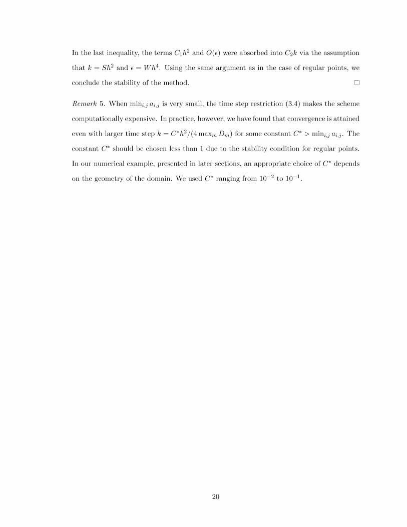
N = 50, 100, 200, 400. Figures 5.1 shows the simulation result of u1 for N = 100.

The convergence rate, r, can be computed as follows:

r =log(E1/E2)

log(h1/h2),

where E1 and E2 are errors between the numerical and the analytic solutions in norms

computed with grid size h1 and h2. The errors and convergence rates are presented in

24

0.5

0

0.5

0.5

0

0.50.2

0.4

0.6

0.8

1

xy

u

Figure 5.1. The solution u1 at T = 1 on a 100× 100 grid.

Table 5.1. Errors and convergence rates of the example simulated in a circular domain forT = 1.

Grid size ‖u− uA‖1 r ‖u− uA‖2 r ‖u− uA‖∞ r

50× 50 1.198× 10−2 − 2.271× 10−2 − 4.733× 10−2 −100× 100 2.859× 10−3 2.07 5.400× 10−3 2.07 1.132× 10−2 2.06

200× 200 7.089× 10−4 2.01 1.337× 10−3 2.01 2.880× 10−3 1.97

400× 400 1.593× 10−4 2.15 3.000× 10−4 2.16 6.398× 10−4 2.17

Table 5.1. As shown in Table 5.1, second-order convergence rates both in L1-, L2- and

L∞-norms are achieved.

We also perform the convergence test for a small time step, T = 0.01. The convergence

rates are summarized in Table 5.2. Note that the convergence rate in the L1-norm is second

order, as predicted by theory.

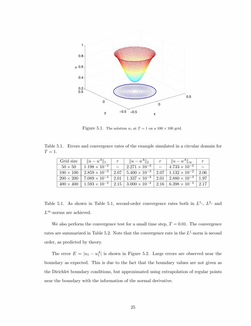
The error E = |u1 − uA1 | is shown in Figure 5.2. Large errors are observed near the

boundary as expected. This is due to the fact that the boundary values are not given as

the Dirichlet boundary conditions, but approximated using extrapolation of regular points

near the boundary with the information of the normal derivative.

25

0.5

0

0.5

0.5

0

0.54

2

0

2

4

6

8x 10 4

x

|uexact unum|

y

|uex

act

unu

m|

Figure 5.2. The absolute error |u1 − uA1 | at T = 0.01 on a 100× 100 grid.

Table 5.2. Errors and convergence rates of the example simulated in a circular domain forT = 0.01.

Grid size ‖u− uA‖1 r ‖u− uA‖2 r ‖u− uA‖∞ r

50× 50 1.330× 10−4 − 3.778× 10−4 − 2.358× 10−3 −100× 100 3.132× 10−5 2.09 8.945× 10−5 2.08 6.613× 10−4 1.83

200× 200 7.777× 10−6 2.01 2.286× 10−5 1.97 2.148× 10−4 1.62

400× 400 1.757× 10−6 2.15 5.026× 10−6 2.19 4.357× 10−5 2.30

26

5.2 Convergence test on an annulus

Next, we consider the reaction-diffusion system on an annulus. This type of domain

may be useful in modeling biochemical signaling in a cell membrane. Note our method

is applicable for domains with arbitrary topology via the level set representation. In this

example, Ω = (x, y)|r21 < x2 + y2 < r22, M = 1 and

f1(x, y, t, u1) = −au1 + exp(−at)(4b2D1(x2 + y2) cos θ + 4bD1 sin θ),

u01(x, y) = 0.2(1 + cos θ),

where θ = θ(x, y) = b(x2 + y2 − r21) and b = π/(r22 − r21). Then uA1 (x, t) = 0.2 exp(−at)(1 +

cos(b(x2 + y2 − r21))) is the analytic solution to (1.1). Also note that the solution satisfies

the Neumann boundary conditions (1.1b) on inner and outer boundaries. The parameter

values are chosen as r1 = 0.2, r2 = 0.4, D1 = 0.1 and a = 0.1. We solve the problem on

a N × N grid until T = 0.01, for N = 50, 100, 200, and 400. The result with N = 100 is

shown in Figure 5.3.

0.5

0

0.5

0.5

0

0.50.2

0.1

0

0.1

0.2

0.3

0.4

xy

u

Figure 5.3. The solution u1 on a 100× 100 grid.

As in the previous example, we performed the convergence rate analysis by calculating

the absolute errors in L1-, L2- and L∞-norms. The method solves the problem with second

order convergence rate in all norms as shown in Table 5.3.

27

Table 5.3. Errors and convergence rates of the example simulated in a circular domainwith a hole.

Grid size ‖u− uA‖1 r ‖u− uA‖2 r ‖u− uA‖∞ r

50× 50 3.467× 10−4 − 7.647× 10−4 − 4.421× 10−3 −100× 100 6.770× 10−5 2.36 1.421× 10−4 2.43 9.167× 10−4 2.27

200× 200 1.595× 10−5 2.09 3.298× 10−5 2.11 2.236× 10−4 2.04

400× 400 3.653× 10−6 2.13 7.581× 10−6 2.12 5.154× 10−5 2.12

5.3 Convergence test of a two-species system

To see how a multi-species system affects the convergence rate of our method, we con-

sider an example of (1.1) in a circular domain Ω = (x, y)|x2 + y2 < R2 with M = 2

and

f1(x, y, t, u1, u2) = −au2 + exp(−at)(4b2D1(x2 + y2) cos θ + 4bD1 sin θ),

f2(x, y, t, u1, u2) = −au1 + exp(−at)(4b2D2(x2 + y2) cos θ + 4bD2 sin θ),

u01(x, y) = cos θ,

u02(x, y) = cos θ,

where θ = θ(x, y) = b(x2 + y2 − R2) and a, b are constants. Then (1.1) has the analytic

solution, uA1 (x, t) = exp(−at) cos(b(x2 + y2 −R2)) and uA2 (x, t) = exp(−at) cos(b(x2 + y2 −

R2)).

In the test, we chose the parameter values R = 0.3, D1 = 0.1, D2 = 0.05, a = 0.1, b = 4π

and final time T = 0.01. The test result in Table 5.4 shows the second order convergence

rate in L1 and L2 as in the single species example.

In order to test whether our method is robust when two diffusion rates are in different

orders of magnitude, we simulated the system with D1 = 0.1 and D2 = 0.001. As shown in

Table 5.5, the convergence rate in L1-norm is maintained to be second order despite a drop

of the convergence rate of u2 in L∞-norm.

28

Table 5.4. Errors and convergence rates of the example with multiple species simulated ina circular domain, when D = (0.1, 0.05).

Grid size ‖u1 − uA1 ‖1 r ‖u1 − uA1 ‖2 r ‖u1 − uA1 ‖∞ r

50× 50 1.330× 10−4 − 3.779× 10−4 − 2.358× 10−3 −100× 100 3.133× 10−5 2.09 8.947× 10−5 2.08 6.614× 10−4 1.83

200× 200 7.779× 10−6 2.01 2.287× 10−5 1.97 2.148× 10−4 1.62

400× 400 1.758× 10−6 2.15 5.027× 10−6 2.19 4.358× 10−5 2.30

Grid size ‖u2 − uA2 ‖1 r ‖u2 − uA2 ‖2 r ‖u2 − uA2 ‖∞ r

50× 50 6.775× 10−5 − 2.188× 10−4 − 1.602× 10−3 −100× 100 1.566× 10−5 2.11 5.130× 10−5 2.09 4.610× 10−4 1.80

200× 200 3.879× 10−6 2.01 1.312× 10−5 1.97 1.518× 10−4 1.60

400× 400 8.777× 10−7 2.14 2.873× 10−6 2.19 3.045× 10−5 2.32

Table 5.5. Errors and convergence rates of the example with multiple species simulated ina circular domain, when D = (0.1, 0.001).

Grid size ‖u1 − uA1 ‖1 r ‖u1 − uA1 ‖2 r ‖u1 − uA1 ‖∞ r

50× 50 1.331× 10−4 − 3.780× 10−4 − 2.359× 10−3 −100× 100 3.133× 10−5 2.09 8.949× 10−5 2.08 6.615× 10−4 1.83

200× 200 7.781× 10−6 2.01 2.287× 10−5 1.97 2.149× 10−4 1.62

400× 400 1.758× 10−6 2.15 5.029× 10−6 2.19 4.358× 10−5 2.30

Grid size ‖u2 − uA2 ‖1 r ‖u2 − uA2 ‖2 r ‖u2 − uA2 ‖∞ r

50× 50 1.745× 10−6 − 9.745× 10−6 − 9.683× 10−5 −100× 100 3.747× 10−7 2.22 2.659× 10−6 1.87 3.759× 10−5 1.37

200× 200 8.475× 10−8 2.14 7.183× 10−7 1.89 1.697× 10−5 1.15

400× 400 1.779× 10−8 2.25 1.487× 10−8 2.27 3.935× 10−6 2.11

29

5.4 A multi-species system in a star-shaped cell

Biochemical reaction between species A and B that creates species C can be described

by the following chemical equation:

A + Bk1k2

C. (5.1)

Here k1 and k2 represent the forward and backward reaction rates, respectively. The above

equation explains many biological processes including receptor-ligand binding [33], protein

complex formation [1] and gene expression [11]. Let u1, u2 and u3 denote the concentration

levels of A,B and C, respectively. To model (5.1) in a diffusive and bounded environment

such as cell and cell membrane, we use the reaction-diffusion system (1) with M = 3 and

f(u) = (f1(u), f2(u), f3(u)) = (k2u3 − k1u1u2, k2u3 − k1u1u2, k1u1u2 − k2u3).

Suppose that the system is defined in the domain Ω enclosed by a curve (x(θ), y(θ))

parametrized by angle in radians:

x(θ) =1

15(5 + sin 5θ) cos θ, y(θ) =

1

15(5 + sin 5θ) sin θ.

The reaction rates and diffusion rates are (D1, D2, D3) = (0.1, 0.001, 0.05) and (k1, k2) =

(10, 0.1). The initial conditions are,

u01 = 1 + cos(3.125π(x2 + y2 − (0.4)2)),

u02 = 1− cos(3.125π(x2 + y2 − (0.4)2)),

u03 = 0.1(1 + cos(3.125π(x2 + y2 − (0.4)2))).

The problem is solved on a N × N grid until T = 0.01, for N = 50, 100, 200, and 400. In

Figures 5.4, 5.5 and 5.6 we show the results for N = 100.

Since the analytical solution is not known for this example, we estimate the convergence

rate by comparing numerical solutions using different grid sizes:

r = log2

(‖uh − uh/2‖‖u2h − uh‖

),

where uh/2, uh and u2h are numerical solutions with grid sizes h/2, h and 2h, respectively.

The result are presented in Table 5.6, which shows the second-order convergence of the

method in the L1- and L2-norms.

30

0.5

0

0.5

0.5

0

0.5

0.5

1

1.5

2

xy

u 1

Figure 5.4. The numerical solution of u1 on a 100× 100 grid.

0.5

0

0.5

0.5

0

0.5

0

0.5

1

xy

u 2

Figure 5.5. The numerical solution of u2 on a 100× 100 grid.

31

0.5

0

0.5

0.5

0

0.50.1

0.12

0.14

0.16

0.18

0.2

0.22

xy

u 3

Figure 5.6. The numerical solution of u3 on a 100× 100 grid.

Table 5.6. Errors and convergence rates of the example simulated in a star-shaped domain.

Grid size ‖uh1 − uh/21 ‖1 r ‖uh1 − u

h/21 ‖2 r ‖uh1 − u

h/21 ‖∞ r

100× 100 8.099× 10−4 − 2.488× 10−3 − 1.914× 10−2 −200× 200 1.764× 10−4 2.20 5.563× 10−4 2.16 4.360× 10−3 2.13

400× 400 4.529× 10−5 1.96 1.447× 10−4 1.94 1.228× 10−3 1.83

Grid size ‖uh2 − uh/22 ‖1 r ‖uh2 − u

h/22 ‖2 r ‖uh2 − u

h/22 ‖∞ r

100× 100 1.318× 10−3 − 7.793× 10−3 − 8.292× 10−2 −200× 200 2.364× 10−4 2.48 2.009× 10−3 1.96 2.940× 10−2 1.50

400× 400 4.868× 10−5 2.28 4.998× 10−4 2.01 1.095× 10−2 2.45

Grid size ‖uh3 − uh/23 ‖1 r ‖uh3 − u

h/23 ‖2 r ‖uh3 − u

h/23 ‖∞ r

100× 100 7.453× 10−5 − 3.046× 10−4 − 3.380× 10−3 −200× 200 1.361× 10−5 2.45 5.460× 10−5 2.48 6.192× 10−4 1.43

400× 400 3.160× 10−6 2.11 1.371× 10−5 1.99 1.882× 10−4 1.72

32

5.5 EphA2/Ephrin-A1 signaling

The temporal evolution of geometric distribution of EphA2 receptors is known to be

important because their lateral transport, which is observed in many cell lines, is signif-

icantly correlated with the tissue invasion potential. The lateral transport of EphA2 is

activated by formulating a complex with Ephrin-A1 ligands. Effects of the spatial distri-

bution of EphA2/Ephrin-A1 complexes to their downstream signaling can be found in [34].

An interesting observation is that the reorganization of actin cytoskeleton may regulate the

geometric distribution of EphA2/Ephrin-A1 complexes. In turn, the downstream signaling

pathways of EphA2/Ephrin-A1 involving the Rho family of GTPases such as RhoA, Rac1

and Cdc42 control the organization of the actin cytoskeleton [10]. Among several proposed

crosstalk schemes of Rho GTPases, the interaction mechanism in Figure 5.7, which we will

be using for modeling, is consistent with the bistability of RhoA, Rac1 and Cdc42 [9], [12].

Cdc42 Rac1 RhoA

EphA2/Ephrin-A1

ActivationInhibition

Figure 5.7. An EphA2/Ephrin-A1 downstream signaling mechanism and the crosstalk between RhoA,

Rac1 and Cdc42.

33

The following biochemical equations describe the signaling mechanism in Figure 5.7:

Ephrin-A1 + EphA2k1k2pEphA2/Ephrin-A1

pEphA2/Ephrin-A1 + RhoAk3k4pEphA2/Ephrin-A1/RhoA

pEphA2/Ephrin-A1/RhoAk5k6pEphA2/Ephrin-A1 + pRhoA

pEphA2/Ephrin-A1 + Rac1k7k8pEphA2/Ephrin-A1/Rac1

pEphA2/Ephrin-A1/Rac1k9k10

pEphA2/Ephrin-A1 + pRac1

pCdc42 + Rac1k11k12

pCdc42/Rac1

pCdc42/Rac1k13k14

pCdc42 + pRac1

pRac1 + RhoAk15k16

pRac1/RhoA

pRac1/RhoAk17k18

pRac1 + pRhoA

pCdc42 + pRhoAk19k20

pCdc42/pRhoA

pCdc42/pRhoAk21k22

Cdc42 + RhoA

Let u1 = [EphA2], u2 = [RhoA], u3 = [pRhoA], u4 = [Rac1], u5 = [pRac1], u6 =

[Cdc42], u7 = [pCdc42], u8 = [pEphA2/Ephrin-A1], u9 = [pRac1/RhoA], u10 =

[pCdc42/Rac1], u11 = [pCdc42/pRhoA], u12 = [pEphA2/Ephrin-A1/RhoA], u13 =

[pEphA2/Ephrin-A1/Rac1] and v = [Ephrin-A1], where [A] denotes the concentration

level of the chemical species A. Given the experimental data of v = [Ephrin-A1], the

reaction-diffusion system (1.1) with M = 13 and the reaction terms:

f1(u) = −k1vu1 + k2u8

f2(u) = −k3u8u2 + k4u12 − k15u5u2 + k16u9 + k21u11 − k22u6u2

f3(u) = k5u12 − k6u8u3 + k17u9 − k18u5u3 − k19u7u3 + k20u11

f4(u) = −k7u8u4 + k8u13 − k11u7u4 + k12u10

f5(u) = k9u13 − k10u8u5 + k13u10 − k14u7u5 − k15u5u2 + k16u9 + k17u9 − k18u5u3

f6(u) = k21u11 − k22u6u2

f7(u) = −k11u7u4 + k12u10 + k13u10 − k14u7u5 − k19u7u3 + k20u11

34

f8(u) = k1vu1 − k2u8 − k3u8u2 + k4u12 + k5u12 − k6u8u3 − k7u8u4 + k8u13

+ k9u13 − k10u8u5

f9(u) = k15u5u2 − k16u9 − k17u9 + k18u5u3

f10(u) = k11u7u4 − k12u10 − k13u10 + k14u7u5

f11(u) = k19u7u3 − k20u11 − k21u11 + k22u6u2

f12(u) = k3u8u2 − k4u12 − k5u12 + k6u8u3

f13(u) = k7u8u4 − k8u13 − k9u13 + k10u8u5

models the spatio-temporal dynamics of the signaling in Figure 5.7. Here we choose

the diffusion rate D = (D1, . . . , D13) with D1, · · · , D7 to be 10−4 and D8, · · · , D13 to

be 5 × 10−5. Reaction rates are given as k = (k1, · · · , k22), where k1, k5, k9, k21 are 1,

k3, k7, k11, k13, k15, k17, k19 are 10−1, and k2n’s are 10−5 for n = 1, · · · , 11. We solved the

reaction-diffusion system in a circular domain Ω = (x, y)|x2 + y2 < (1/3)2 until T = 10,

with initial values u0(x) = (u01(x), · · · , u013(x)) = (10, 5, 0.1, 5, 0.1, 5, 0.1, 0.1, 1, 1, 1, 1, 1) for

all x ∈ Ω. Note that the concentration level of Ephrin-A1, v, which is given as data, works as

an input for the reaction-diffusion system. As the spatial distribution of v evolves over time,

the high concentration regions of pRac1, activated by pEphA2/Ephrin-A1, are collocated

with those of Ephrin-A1 as shown in Figure 5.8. Due to the clustering behavior of Ephrin-

A1, the high concentration regions of pRac1 are centralized despite the diffusion effect. On

the other hand the concentration level of Cdc42 near the center of the cell decreases over

time since RhoA, activated by pEphA2/Ephrin-A1, inhibits Cdc42. These demonstrate the

effects of the spatio-temporal dynamics of Ephrin-A1 to that of its downstream signaling

molecules.

35

Figure 5.8. The first column shows the experimental data of Ephrin-A1 (courtesy of Jay T. Groves). The

second and third columns are numerical solutions of pRac1 and pCdc42, respectively on a 200 × 200 grid.

Rows represent the results at T = 2.5, T = 5, T = 7.5 and T = 10 from top to bottom.

36

Chapter 6

Conclusion

We have proposed a stable second-order accurate method that preserves the non-

negativity of the solution with the Neumann boundary conditions on irregular domains. In

the spatial discretization, the slopes of normal vectors allow us to extrapolate the solutions

inside the domain to approximate the solution on the boundary with third order accuracy.

The algorithm employs adaptive time steps, and is well-posed due to the quasi-positivity

(A1), to enforce the numerical solution of (1.1) to remain in [0,+∞)M . In addition, we

proved that the method is stable. Numerical examples demonstrates that the method has

second-order convergence rate in the L1-norm, and is robust to domain geometry and to

different scales of diffusion rates.

The test involving the EphA2/Ephrin-A1 signaling in a tumor cell, for instance, suggests

that our method may serve as a useful simulation tool for testing biological and physical

hypotheses in biochemical network in cells.

Our spatial discretization may be applicable to the moving domain problem. In the

future, we plan to embed our algorithm within a moving interface using the level set

method [27], [28], [37]. The three-dimensional problem and the surface diffusion prob-

lem are interesting topics to pursue further, applying our stable and non-negative invariant

algorithm.

37

References

[1] K. Amonlirdviman, N. A. Khare, D. R. P. Tree, W.-S. Chen, J. D. Axelrod, and C. J. Tomlin, “Math-

ematical modeling of planar cell polarity to understand domineering nonautonomy,” Science, vol. 307,

pp. 423–426, January 2005.

[2] L.-T. Cheng and Y.-H. R. Tsai, “Redistancing by flow of time dependent Eikonal equation,” J. Comput.

Phys., vol. 227, no. 8, pp. 4002–4017, 2008.

[3] J. Crank and P. Nicolson, “A practical method for numerical evaluation of solutions of partial differential

equations of the heat conduction type,” P. Camb. Philol. Soc., vol. 43, pp. 50–67, 1947.

[4] R. P. Fedkiw, T. Aslam, B. Merriman, and S. Osher, “A non-oscilatory Eulerian approach to interfaces

in multimaterial flows (the Ghost Fluid Method),” J. Comput. Phys., vol. 152, pp. 457–492, 1999.

[5] R. A. Fisher, “The wave of advance of advantageous genes,” Ann. Eugenic., vol. 7, pp. 355–369, 1937.

[6] A. L. Fogelson and J. P. Keener, “Immersed interface methods for Neumann and related problems in

two and three dimensions,” SIAM J. Sci. Comput., vol. 22, no. 5, pp. 1630–1654, 2000.

[7] F. Gibou and R. P. Fedkiw, “A fourth order accurate discretization for the laplace and heat equations on

arbitrary domains, with applications to the Stefan problem,” J. Comput. Phys., vol. 202, pp. 577–601,

2005.

[8] F. Gibou, R. P. Fedkiw, L.-T. Cheng, and M. Kang, “A second-order-accurate symmetric discretization

of the Poisson equation on irregular domains,” J. Comput. Phys., vol. 176, pp. 205–227, 2002.

[9] E. Giniger, “How do Rho family GTPases direct axon growth and guidance? a proposal relating

signaling pathways to growth cone mechanics,” Differentiation, vol. 70, pp. 385–396, 2002.

[10] A. Hall, “Rho GTPases and the actin cytoskeleton,” Science, vol. 279, pp. 509–514, 1998.

[11] J. Hasty, J. Pradines, M. Dolnik, and J. J. Collins, “Noise-based switches and amplifiers for gene

expression,” Proc. Natl. Acad. Sci. USA, vol. 97, no. 5, pp. 2075–2080, 2000.

[12] A. Jilkine, A. F. M. Maree, and L. Edelsetin-Keshet, “Mathematical model for spatial segregation of

the Rho-family GTPases based on inhibitory crosstalk,” B. Math. Biol., vol. 69, pp. 1943–1978, 2007.

[13] H. Johansen and P. Colella, “A Cartesian grid embedded boundary method for Poisson’s equation on

irregular domains,” J. Comput. Phys., vol. 147, pp. 60–85, 1998.

[14] C. Johnson, Numerical Solution of Partial Differential Equations by the Finite Element Method. Cam-

bridge University Press, New York, 1987.

[15] B. N. Kholodenko, “Cell-signalling dynamics in time and space,” Nat. Rev. Mol. Cell Biol., vol. 7, pp.

165–176, 2006.

[16] R. Klajn, M. Fialkowski, I. T. Bensemann, A. Bitner, C. J. Campbell, K. Bishop, S. Smoukov, and

B. A. Grzybowski, “Multicolour micropatterning of thin films of dry gels,” Nat. Mater., vol. 3, pp.

729–735, 2004.

38

[17] A. J. Koch and H. Meinhardt, “Biological pattern formation: from basic mechanisms to complex

structures,” Rev. Mod. Phys., vol. 66, no. 4, pp. 1481–1507, October 1994.

[18] K.-J. Lee, W. D. McCormick, J. E. Pearson, and H. L. Swinney, “Experimental observation of self-

replicating spots in a reaction-diffusion system,” Nature, vol. 369, pp. 215–218, 1994.

[19] R. J. Leveque and Z. Li, “The immersed interface method for Elliptic equation with discontinuous

constants and singular sources,” SIAM J. Numer. Anal., vol. 31, no. 4, pp. 1019–1044, 1994.

[20] J. H. Lightboune, III and R. H. Martin, Jr., “Relatively continuous nonlinear perturbations of analytic

semigroups,” Nonlinear Anal.-Theor., vol. 1, no. 3, pp. 277–292, 1977.

[21] R. H. Martin, Jr., “Nonlinear perturbations of linear evolution systems,” J. Math. Soc. Jpn., vol. 29,

no. 2, pp. 233–252, 1977.

[22] ——, “Abstract functional differential equations and reaction-diffusion systems,” T. Am. Math. Soc.,

vol. 321, no. 1, pp. 1–44, 1990.

[23] P. McCorquodale, P. Colella, and H. Johansen, “A Cartesian grid embedded boundary method for the

heat equation on irregular domains,” J. Comput. Phys., vol. 173, pp. 620–635, 2001.

[24] C. Min and F. Gibou, “Geometric integration over irregular domains with application to level-set

methods,” J. Comput. Phys., vol. 226, pp. 1432–1443, 2007.

[25] K. W. Morton and D. F. Mayers, Numerical Solution of Partial Differential Equations. Cambridge

University Press, New York, 1995.

[26] J. D. Murray, Mathematical Biology II: Spatial Models and Biomedical Applications, 3rd ed. Springer,

New York, 2003.

[27] S. Osher and J. A. Sethian, “Fronts propagating with curvature-dependent speed: algorithms based on

Hamilton-Jacobi formulations,” J. Comput. Phys., vol. 79, pp. 12–49, 1988.

[28] S. J. Osher and R. P. Fedkiw, Level Set Methods and Dynamic Implicit Surfaces, 1st ed. Springer,

New York, 2002.

[29] J. Papac, F. Gibou, and C. Ratsch, “Efficient symmetric discretization for the Poisson, heat and Stefan-

type problems with Robin boundary conditions,” J. Comput. Phys., vol. 229, pp. 875–889, 2010.

[30] D. W. Peaceman and H. H. Rachford Jr., “The numerical solution of parabolic and elliptic differential

equations,” J. Soc. Ind. Appl. Math., vol. 3, no. 1, pp. 28–41, 1955.

[31] M. Pierre, “Global existence in reaction-diffusion systems with control of mass: a survey,” Milan J.

Math., vol. 78, pp. 417–455, 2010.

[32] M. Pierre and D. Schmitt, “Blowup in reaction-diffusion systems with dissipation of mass,” SIAM Rev.,

vol. 42, no. 1, pp. 93–106, 2000.

[33] S. Y. Qi, J. T. Groves, and A. K. Chakraborty, “Synaptic pattern formation during cellular recognition,”

Proc. Natl. Acad. Sci. USA, vol. 98, no. 12, pp. 6548–6553, 2001.

39

[34] K. Salaita, P. M. Nair, R. S. Petit, R. M. Neve, D. Das, J. W. Gray, and J. T. Groves, “Restriction

of receptor movement alters cellular response: physical force sensing by EphA2,” Science, vol. 327, pp.

1380–1385, 2010.

[35] P. Schwartz, D. Adalsteinsson, P. Colella, A. P. Arkin, and M. Onsum, “Numerical computation of

diffusion on a surface,” Proc. Natl. Acad. Sci. USA, vol. 102, no. 32, pp. 11 151–11 156, August 2005.

[36] P. Schwartz, M. Barad, P. Colella, and T. Ligocki, “A Cartesian grid embedded boundary method for

the heat equation and Poisson’s equation in three dimensions,” J. Comput. Phys., vol. 211, pp. 531–550,

2006.

[37] J. A. Sethian, Level Set Methods and Fast Marching Methods: Evolving Interfaces in Computational

Geometry, Fluid Mechanics, Computer Vision, and Materials Science, 2nd ed. Cambridge University

Press, New York, 1999.

[38] C.-W. Shu and S. Osher, “Efficient implementation of essentially non-oscillatory shock-capturing

schemes,” J. Comput. Phys., vol. 77, pp. 439–471, 1988.

[39] ——, “Efficient implementation of essentially non-oscillatory shock-capturing schemes, II,” J. Comput.

Phys., vol. 83, pp. 32–78, 1989.

[40] W. Strychalski, D. Adalsteinsson, and T. Elston, “A cut-cell method for simulating spatial models of

biochemical reaction networks in arbitrary geometries,” Comm. App. Math. Comp. Sci., vol. 5, no. 1,

pp. 31–53, 2010.

[41] Y.-H. R. Tsai, “Rapid and accurate computation of the distance function using grids,” J. Comput.

Phys., vol. 178, pp. 175–195, 2002.

[42] A. M. Turing, “The chemical basis of morphogenesis,” Philos. T. Roy. Soc. B, vol. 237, pp. 37–72, 1952.

[43] C. W. Wolgemuth and M. Zajac, “The moving boundary node method: a level set-based, finite volume

algorithm with applications to cell motility,” J. Comput. Phys., vol. 229, pp. 7287–7308, 2010.

40