A Scalable and Cost Effective Architecture for High

Gain Beamforming Antennas

Omar Bakr

Electrical Engineering and Computer SciencesUniversity of California at Berkeley

Technical Report No. UCB/EECS-2010-178

http://www.eecs.berkeley.edu/Pubs/TechRpts/2010/EECS-2010-178.html

December 23, 2010

Copyright © 2010, by the author(s).All rights reserved.

Permission to make digital or hard copies of all or part of this work forpersonal or classroom use is granted without fee provided that copies arenot made or distributed for profit or commercial advantage and that copiesbear this notice and the full citation on the first page. To copy otherwise, torepublish, to post on servers or to redistribute to lists, requires prior specificpermission.

A Scalable and Cost Effective Architecture for High Gain BeamformingAntennas

by

Omar Mohammed Bakr

A dissertation submitted in partial satisfaction of the

requirements for the degree of

Doctor of Philosophy

in

Computer Science

in the

Graduate Division

of the

University of California, Berkeley

Committee in charge:

Professor Ali M. Niknejad, ChairProfessor Eric A. BrewerProfessor Paul K. Wright

Fall 2010

A Scalable and Cost Effective Architecture for High Gain BeamformingAntennas

Copyright 2010by

Omar Mohammed Bakr

1

Abstract

A Scalable and Cost Effective Architecture for High Gain Beamforming Antennas

by

Omar Mohammed Bakr

Doctor of Philosophy in Computer Science

University of California, Berkeley

Professor Ali M. Niknejad, Chair

Many state-of-the-art wireless systems, such as long distance networks (point-to-point,point-to-multipoint, and mesh) and high bandwidth networks using mm-wave frequencies,require high gain antennas to overcome adverse channel conditions. These networks couldbe greatly aided by adaptive beamforming antenna arrays, which can significantly simplifythe installation and maintenance costs (e.g., by enabling automatic beam alignment), andimprove the capacity of these networks. Such networks typically require gains ranging from20-30dBi with wide scanning range in both dimensions. To achieve this, arrays with hundredsor even thousands of antennas are required, which cannot be done with existing techniquesthat do not scale very well beyond 10-20 antennas.

In this dissertation, we examine and address the main challenges presented by large ar-rays, starting from electromagnetic/antenna and radio circuit design and proceeding to thesignal processing and algorithms domain. We propose 3-dimensional antenna array structuresthat realize large gains and scan angles at a much reduced size and form factor compared withconventional planar antennas. At the circuit level, we propose a hybrid RF/digital beam-forming radio architecture that takes advantage of low cost silicon integration to reduce theoverall component count and power consumption levels of the system without limiting thecapacity. We consider different techniques for implementing compact beamformers reliablyat high radio frequencies, and present signal processing techniques based on adaptive filteringmethods for optimizing those beamformers. The performance implications of low precisionanalog beamformers and implementation errors are also analyzed and quantified, and com-putationally efficient vector quantization techniques that take advantage of the size and scaleof the arrays to compensate for low precision are proposed. We validate our approach withmathematical proofs and computer simulations.

i

To my mentor and friend.

ii

Contents

List of Figures v

List of Tables ix

1 Introduction 11.1 The wireless revolution . . . . . . . . . . . . . . . . . . . . . . . . . . . . . . 11.2 Rural connectivity and the digital divide . . . . . . . . . . . . . . . . . . . . 11.3 Challenges for growing and expanding the reach of wireless networks . . . . . 21.4 Wireless networks today . . . . . . . . . . . . . . . . . . . . . . . . . . . . . 41.5 Adaptive beamforming systems . . . . . . . . . . . . . . . . . . . . . . . . . 51.6 High gain beamforming systems . . . . . . . . . . . . . . . . . . . . . . . . . 91.7 Research goals and contributions . . . . . . . . . . . . . . . . . . . . . . . . 91.8 Organization of the Dissertation . . . . . . . . . . . . . . . . . . . . . . . . . 10

2 Background 112.1 Antenna basics . . . . . . . . . . . . . . . . . . . . . . . . . . . . . . . . . . 11

2.1.1 Antenna radiation patterns . . . . . . . . . . . . . . . . . . . . . . . 112.1.2 Directivity . . . . . . . . . . . . . . . . . . . . . . . . . . . . . . . . . 122.1.3 Antenna effciency . . . . . . . . . . . . . . . . . . . . . . . . . . . . . 162.1.4 Antenna bandwidth . . . . . . . . . . . . . . . . . . . . . . . . . . . . 172.1.5 Polarization . . . . . . . . . . . . . . . . . . . . . . . . . . . . . . . . 172.1.6 Free space propagation . . . . . . . . . . . . . . . . . . . . . . . . . . 18

2.2 Static versus steerable antennas . . . . . . . . . . . . . . . . . . . . . . . . . 202.2.1 Other types of antenna arrays . . . . . . . . . . . . . . . . . . . . . . 252.2.2 Scanning versus adaptive arrays . . . . . . . . . . . . . . . . . . . . . 25

2.3 The wireless channel . . . . . . . . . . . . . . . . . . . . . . . . . . . . . . . 262.3.1 Channel fading . . . . . . . . . . . . . . . . . . . . . . . . . . . . . . 272.3.2 Channel diversity . . . . . . . . . . . . . . . . . . . . . . . . . . . . . 322.3.3 Frequency selective channels . . . . . . . . . . . . . . . . . . . . . . . 332.3.4 Spatial multiplexing . . . . . . . . . . . . . . . . . . . . . . . . . . . 34

3 Radio architectures 363.1 Comparison of Architecture . . . . . . . . . . . . . . . . . . . . . . . . . . . 36

3.1.1 Hybrid arrays . . . . . . . . . . . . . . . . . . . . . . . . . . . . . . . 393.2 RF beamformer design . . . . . . . . . . . . . . . . . . . . . . . . . . . . . . 41

iii

3.2.1 A multi-input/multi-output RF beamforming module . . . . . . . . . 413.2.2 Signal combining/splitting . . . . . . . . . . . . . . . . . . . . . . . . 463.2.3 RF phase shifting and complex multiplication techniques . . . . . . . 473.2.4 Vector combining complex multiplier implementation . . . . . . . . . 55

3.3 Conslusion . . . . . . . . . . . . . . . . . . . . . . . . . . . . . . . . . . . . . 59

4 Antenna designs 624.1 Array factor and radiation pattern calculations . . . . . . . . . . . . . . . . . 63

4.1.1 Impact of antenna spacing . . . . . . . . . . . . . . . . . . . . . . . . 634.1.2 Impact of array geometry . . . . . . . . . . . . . . . . . . . . . . . . 644.1.3 Planar arrays . . . . . . . . . . . . . . . . . . . . . . . . . . . . . . . 664.1.4 Side lobes . . . . . . . . . . . . . . . . . . . . . . . . . . . . . . . . . 724.1.5 Antenna coupling . . . . . . . . . . . . . . . . . . . . . . . . . . . . . 73

4.2 3-dimensional arrays . . . . . . . . . . . . . . . . . . . . . . . . . . . . . . . 754.2.1 Lobe cancellation . . . . . . . . . . . . . . . . . . . . . . . . . . . . . 77

5 Adaptive beamforming and channel estimation 825.1 Adaptive filter techniques . . . . . . . . . . . . . . . . . . . . . . . . . . . . 83

5.1.1 Gradient descent . . . . . . . . . . . . . . . . . . . . . . . . . . . . . 855.1.2 Other adaptive filtering techniques . . . . . . . . . . . . . . . . . . . 87

5.2 Channel Estimation via Adaptive Filtering . . . . . . . . . . . . . . . . . . . 875.2.1 Performance evaluation . . . . . . . . . . . . . . . . . . . . . . . . . . 89

5.3 Null-steering . . . . . . . . . . . . . . . . . . . . . . . . . . . . . . . . . . . . 935.4 Adaptive filtering with interference cancellation . . . . . . . . . . . . . . . . 995.5 Frequency synchronization . . . . . . . . . . . . . . . . . . . . . . . . . . . . 1035.6 Multi-beam (multi-receiver) arrays . . . . . . . . . . . . . . . . . . . . . . . 1055.7 Transmit beamforming . . . . . . . . . . . . . . . . . . . . . . . . . . . . . . 1075.8 Conclusion . . . . . . . . . . . . . . . . . . . . . . . . . . . . . . . . . . . . . 109

6 Beamforming performance with weight errors 1106.1 Beamforming . . . . . . . . . . . . . . . . . . . . . . . . . . . . . . . . . . . 111

6.1.1 Analysis of Imperfect Phase Shifts . . . . . . . . . . . . . . . . . . . . 1126.1.2 Simulation Results . . . . . . . . . . . . . . . . . . . . . . . . . . . . 1136.1.3 Worst case performance analysis . . . . . . . . . . . . . . . . . . . . . 116

6.2 Beam-nulling . . . . . . . . . . . . . . . . . . . . . . . . . . . . . . . . . . . 1216.2.1 Analysis of Errors in Weights . . . . . . . . . . . . . . . . . . . . . . 1226.2.2 Simulation Results . . . . . . . . . . . . . . . . . . . . . . . . . . . . 125

6.3 Conclusion . . . . . . . . . . . . . . . . . . . . . . . . . . . . . . . . . . . . . 125

7 Error mitigation with vector quantization 1327.1 Quantization problem statement . . . . . . . . . . . . . . . . . . . . . . . . . 1337.2 Scalar quantization of beamforming weights . . . . . . . . . . . . . . . . . . 134

7.2.1 Spatial matched filter . . . . . . . . . . . . . . . . . . . . . . . . . . . 1357.2.2 Zero-Forcing beamformer . . . . . . . . . . . . . . . . . . . . . . . . . 137

7.3 Vector quantization of antenna weights . . . . . . . . . . . . . . . . . . . . . 156

iv

7.3.1 An approximate lower bound on achievable SIR . . . . . . . . . . . . 1567.3.2 Constructive algorithms for improving interference suppression . . . . 1757.3.3 Improving the beamforming gain using vector quantization . . . . . . 201

7.4 Conclusion . . . . . . . . . . . . . . . . . . . . . . . . . . . . . . . . . . . . . 205

8 Conclusion and future work 209

Bibliography 211

v

List of Figures

1.1 Long distance wireless networks for rural connectivity . . . . . . . . . . . . . 31.2 Mobile data traffic . . . . . . . . . . . . . . . . . . . . . . . . . . . . . . . . 31.3 Antenna pattern options . . . . . . . . . . . . . . . . . . . . . . . . . . . . . 61.4 Network sectorization and cell splitting . . . . . . . . . . . . . . . . . . . . 71.5 Adaptive beamforming antennas . . . . . . . . . . . . . . . . . . . . . . . . . 8

2.1 3D antenna radiation pattern plots . . . . . . . . . . . . . . . . . . . . . . . 132.2 2D antenna radiation pattern plots . . . . . . . . . . . . . . . . . . . . . . . 142.3 Basic antennas patterns . . . . . . . . . . . . . . . . . . . . . . . . . . . . . 152.4 Free space path loss . . . . . . . . . . . . . . . . . . . . . . . . . . . . . . . . 182.5 Phase response of a uniform linear array . . . . . . . . . . . . . . . . . . . . 212.6 Linear array pattern . . . . . . . . . . . . . . . . . . . . . . . . . . . . . . . 232.7 Switched antenna array . . . . . . . . . . . . . . . . . . . . . . . . . . . . . . 262.8 2x2 MIMO scenario . . . . . . . . . . . . . . . . . . . . . . . . . . . . . . . . 34

3.1 Radio architectures for beamforming . . . . . . . . . . . . . . . . . . . . . . 373.2 Hybrid beamforming architectures . . . . . . . . . . . . . . . . . . . . . . . . 423.3 Multi-input/multi-output RF frontend . . . . . . . . . . . . . . . . . . . . . 433.4 Hybrid RF beamforming chip on a PCB . . . . . . . . . . . . . . . . . . . . 433.5 Transmit/Receive building blocks . . . . . . . . . . . . . . . . . . . . . . . . 453.6 Multi-input/Multi-output RF complex multiplier block . . . . . . . . . . . . 453.7 Power combining structures . . . . . . . . . . . . . . . . . . . . . . . . . . . 483.8 Wilkinson power combiner measurements (Part 1) . . . . . . . . . . . . . . . 493.9 Wilkinson power combiner measurements . . . . . . . . . . . . . . . . . . . . 503.10 Reflective-type phase shifters . . . . . . . . . . . . . . . . . . . . . . . . . . . 513.11 Switched transmission line phase shifter . . . . . . . . . . . . . . . . . . . . . 533.12 Vector combining based phase rotator . . . . . . . . . . . . . . . . . . . . . . 543.13 Polyphase filter networks . . . . . . . . . . . . . . . . . . . . . . . . . . . . . 573.14 Wideband 4-stage polyphase network . . . . . . . . . . . . . . . . . . . . . . 583.15 Gain control (digital implementation) . . . . . . . . . . . . . . . . . . . . . . 593.16 Programable gain block (unit cell architecture) . . . . . . . . . . . . . . . . . 60

4.1 Impact of number of antennas/antenna spacing on the array pattern . . . . . 654.2 Broadside/endfire configurations of a linear array . . . . . . . . . . . . . . . 664.3 Impact of array geometry on beamwidth and pattern shape . . . . . . . . . . 67

vi

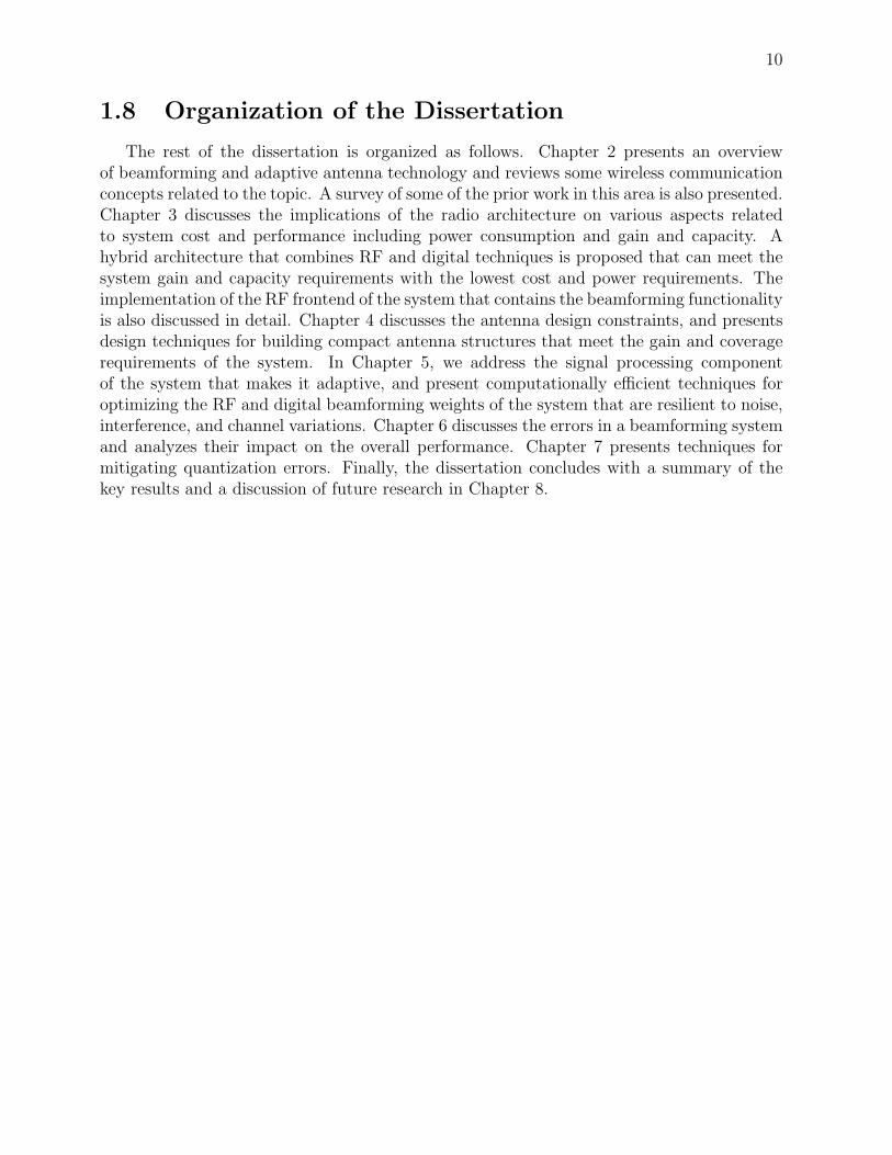
4.4 Broadside versus endfire azimuth beamwidth . . . . . . . . . . . . . . . . . . 684.5 Beam pattern of a linear array for different steering vectors . . . . . . . . . . 694.6 Array response versus frequency . . . . . . . . . . . . . . . . . . . . . . . . . 714.7 Azimuth endfire pattern of rectangular arrays . . . . . . . . . . . . . . . . . 724.8 Side lobe level versus array geometry . . . . . . . . . . . . . . . . . . . . . . 734.9 Dipole radiation pattern (polar plot) . . . . . . . . . . . . . . . . . . . . . . 744.10 3-dimensional rectangular array of monopoles . . . . . . . . . . . . . . . . . 784.11 3-dimensional cylindrical array of monopoles . . . . . . . . . . . . . . . . . . 794.12 Patch arrays . . . . . . . . . . . . . . . . . . . . . . . . . . . . . . . . . . . . 804.13 3D array layout with λ/4 shifting . . . . . . . . . . . . . . . . . . . . . . . . 804.14 Lobe cancellation using λ/4 spacing . . . . . . . . . . . . . . . . . . . . . . . 81

5.1 Block diagram for a generic adaptive filter . . . . . . . . . . . . . . . . . . . 865.2 System identification via adaptive filtering . . . . . . . . . . . . . . . . . . . 885.3 Channel estimation through adaptive filtering (receive beamforming) . . . . 905.4 Adaptive filter beamforming performance without noise . . . . . . . . . . . . 925.5 Adaptive filter beamforming performance with noise (NLMS) . . . . . . . . . 945.6 Adaptive filter beamforming performance with noise (sign-LMS) . . . . . . . 955.7 Adaptive filter beamforming performance with channel variation . . . . . . . 965.8 Interference cancellation scenario . . . . . . . . . . . . . . . . . . . . . . . . 975.9 Beam-nulling using the LMS algorithm . . . . . . . . . . . . . . . . . . . . . 1005.10 Beam-nulling using the LMS algorithm with time-varying channels . . . . . . 1015.11 Channel estimation through adaptive filtering with known interferers . . . . 1035.12 Iterative beam-nulling using the LMS algorithm . . . . . . . . . . . . . . . . 1045.13 DMMSE vs LMS in the presence of frequency offsets . . . . . . . . . . . . . 1065.14 Computation of digital beamforming weights . . . . . . . . . . . . . . . . . . 1085.15 Channel estimation through adaptive filtering (transmit beamforming) . . . 109

6.1 LOS beamforming scenario . . . . . . . . . . . . . . . . . . . . . . . . . . . . 1116.2 Beamforming gain as a function of phase errors . . . . . . . . . . . . . . . . 1146.3 Simulated beamforming gain for different phase errors distributions . . . . . 1156.4 Array patterns with quantization (Part 1) . . . . . . . . . . . . . . . . . . . 1176.5 Array patterns with quantization (Part 2) . . . . . . . . . . . . . . . . . . . 1186.6 Array patterns with quantization (Part 3) . . . . . . . . . . . . . . . . . . . 1196.7 Spatial domain wireless channel representation . . . . . . . . . . . . . . . . . 1236.8 Mean square error angle σ2

θ versus weight errors . . . . . . . . . . . . . . . . 1266.9 Average interferer power in the presence of errors . . . . . . . . . . . . . . . 1276.10 Average desired power (beamforming gain) in the presence of errors . . . . . 1286.11 Cosine angle approximation for the beamforming gain . . . . . . . . . . . . . 1296.12 Cosine angle approximation for the beamforming gain . . . . . . . . . . . . . 130

7.1 SIR under QMF (Rayleigh channel, Part 1) . . . . . . . . . . . . . . . . . . 1387.2 SIR under QMF (Rayleigh channel, Part 2) . . . . . . . . . . . . . . . . . . 1397.3 Desired signal under QMF (Rayleigh channel, Part 1) . . . . . . . . . . . . . 1407.4 Desired signal under QMF (Rayleigh channel, Part 2) . . . . . . . . . . . . . 141

vii

7.5 Interferer power under QMF (Rayleigh channel, Part 1) . . . . . . . . . . . . 1427.6 Interferer power under QMF (Rayleigh channel, Part 2) . . . . . . . . . . . . 1437.7 SIR under QMF (LOS channel/uniform linear array, Part 1) . . . . . . . . . 1447.8 SIR under QMF (LOS channel/uniform linear array, Part 2) . . . . . . . . . 1457.9 Desired signal under QMF (LOS channel/uniform linear array, Part 1) . . . 1467.10 Desired signal under QMF (LOS channel/uniform linear array, Part 2) . . . 1477.11 Interferer power under QMF (LOS channel/uniform linear array, Part 1) . . 1487.12 Interferer power under QMF (LOS channel/uniform linear array, Part 2) . . 1497.13 SIR under QMF (LOS channel/uniform square array, Part 1) . . . . . . . . . 1507.14 SIR under QMF (LOS channel/uniform square array, Part 2) . . . . . . . . . 1517.15 Desired signal under QMF (LOS channel/uniform square array, Part 1) . . . 1527.16 Desired signal under QMF (LOS channel/uniform square array, Part 2) . . . 1537.17 Interferer power under QMF (LOS channel/uniform square array, Part 1) . . 1547.18 Interferer power under QMF (LOS channel/uniform square array, Part 2) . . 1557.19 SIR under QZF (Rayleigh channel, Part 1) . . . . . . . . . . . . . . . . . . . 1577.20 SIR under QZF (Rayleigh channel, Part 2) . . . . . . . . . . . . . . . . . . . 1587.21 Desired signal under QZF (Rayleigh channel, Part 1) . . . . . . . . . . . . . 1597.22 Desired signal under QZF (Rayleigh channel, Part 2) . . . . . . . . . . . . . 1607.23 Interferer power under QZF (Rayleigh channel, Part 1) . . . . . . . . . . . . 1617.24 Interferer power under QZF (Rayleigh channel, Part 2) . . . . . . . . . . . . 1627.25 SIR under QZF (LOS channel/uniform linear array, Part 1) . . . . . . . . . 1637.26 SIR under QZF (LOS channel/uniform linear array, Part 2) . . . . . . . . . 1647.27 Desired signal under QZF (LOS channel/uniform linear array, Part 1) . . . . 1657.28 Desired signal under QZF (LOS channel/uniform linear array, Part 2) . . . . 1667.29 Interferer power under QZF (LOS channel/uniform linear array, Part 1) . . . 1677.30 Interferer power under QZF (LOS channel/uniform linear array, Part 2) . . . 1687.31 SIR under QZF (LOS channel/uniform square array, Part 1) . . . . . . . . . 1697.32 SIR under QZF (LOS channel/uniform square array, Part 2) . . . . . . . . . 1707.33 Desired signal under QZF (LOS channel/uniform square array, Part 1) . . . 1717.34 Desired signal under QZF (LOS channel/uniform square array, Part 2) . . . 1727.35 Interferer power under QZF (LOS channel/square linear array, Part 1) . . . 1737.36 Interferer power under QZF (LOS channel/square linear array, Part 2) . . . 1747.37 Average SIR under the GCD algorithm (Rayleigh, Part 1) . . . . . . . . . . 1777.38 Average SIR under the GCD algorithm (Rayleigh, Part 2) . . . . . . . . . . 1787.39 Average desired signal under the GCD algorithm (Rayleigh, Part 1) . . . . . 1797.40 Average desired signal under the GCD algorithm (Rayleigh, Part 2) . . . . . 1807.41 Average interferer power under the GCD algorithm (Rayleigh, Part 1) . . . . 1817.42 Average interferer power under the GCD algorithm (Rayleigh, Part 2) . . . . 1827.43 Average SIR under the iGCD algorithm (Rayleigh, Part 1) . . . . . . . . . . 1847.44 Average SIR under the iGCD algorithm (Rayleigh, Part 2) . . . . . . . . . . 1857.45 Average desired signal under the iGCD algorithm (Rayleigh, Part 1) . . . . . 1867.46 Average desired signal under the iGCD algorithm (Rayleigh, Part 2) . . . . . 1877.47 Average interferer power under the iGCD algorithm (Rayleigh, Part 1) . . . 1887.48 Average interferer power under the iGCD algorithm (Rayleigh, Part 2) . . . 1897.49 Average SIR under the LSB-GCD algorithm (Rayleigh, Part 1) . . . . . . . . 191

viii

7.50 Average SIR under the LSB-GCD algorithm (Rayleigh, Part 2) . . . . . . . . 1927.51 Average desired signal under the LSB-GCD algorithm (Rayleigh, Part 1) . . 1937.52 Average desired signal under the LSB-GCD algorithm (Rayleigh, Part 2) . . 1947.53 Average interferer power under the LSB-GCD algorithm (Rayleigh, Part 1) . 1957.54 Average interferer power under the LSB-GCD algorithm (Rayleigh, Part 2) . 1967.55 Comparison of vector quantization algorithms . . . . . . . . . . . . . . . . . 1977.56 iGCD under different channel models . . . . . . . . . . . . . . . . . . . . . . 1987.57 GCD performance with different initializations . . . . . . . . . . . . . . . . . 1997.58 SIR under exhaustive search . . . . . . . . . . . . . . . . . . . . . . . . . . . 2007.59 SIR under GCD for switched antenna arrays . . . . . . . . . . . . . . . . . . 2027.60 Interference power under GCD for switched antenna arrays . . . . . . . . . . 2037.61 Desired signal power under GCD algorithm for switched antenna arrays . . . 2047.62 Beamforming gain (GCD versus scalar quantization) . . . . . . . . . . . . . 2067.63 Beamforming gain (GCD versus exhaustive search) . . . . . . . . . . . . . . 2077.64 Beamforming gain under the GCD algorithm with different initializations . . 208

ix

List of Tables

4.1 Simulated azimuth beamwidths of broadside and endfire linear arrays . . . . 694.2 Simulated array gain versus the spacing between antennas . . . . . . . . . . 75

x

Acknowledgments

“Dear Rich,It has been over four years since we last spoke. I still remember that conversation as if it

had happened yesterday. There was a lot more I wanted to say, but did not realize that thisconversation was going to be our last. So I will try to do my best to express my thoughts ina few words.

The last seven years are by far the most special. Meeting you and working with youwas THE highlight of it all. I learned a lot from you in a very short period of time. Mostimportantly, you taught me how to think big, how science and engineering can be a greatinstrument for changing the world to the better, and how I can do it all while having thetime of my life. Thank you for giving me this opportunity. Thank you for your patienceand confidence in me. It helped a lot every time I faced a new challenge knowing that youbelieved I can take it on.

I cannot express enough my feelings of gratitude. However, there is another reason whyI am writing this to you. I have no doubt that you remember (you never forget) that whenwe last talked, I asked you “Rich, what can I do?” Your answer was “You can finish yourdissertation!”. That was your last request. Well here it is. It took a little longer than youwould have liked, but we finally made it, and I say “we” because your advice and guidancewere key in making it this far.

Although Rich I feel relieved that this is over, the real journey has only begun. It’s ajourney to give back, a journey to make a difference in the lives of others like you made adifference in mine, a journey that I had never thought I would embark on without you, butlife is a full of surprises. I have seen you accomplish a lot in so little time. I would have beenmore than content with a fraction of that, but now I know that you expect nothing less.

Rest in peace my friend, and Go Bears!”

Well, it was a great journey, probably the most exciting and stimulating of my life. I amvery fortunate that I did not have to travel alone. By the grace of God, I was always blessedwith great companions throughout the journey, and would like to express my gratitude toeach and every one of them.

I cannot imagine making it this far in life without the unconditional love and support Ireceived from my parents. Every morning I wake up, I feel very confident knowing I couldalways count on their prayers and knowing that they are always behind me. They always putmy happiness and well being before everything. From the moment I opened my eyes, theirlives revolved around mine (that may have changed a little bit after their first grandchildwas born). Most importantly, they gave me a great brother and two great sisters. Together,we make a great team.

I was very fortunate to have the Blue & Gold blood run in my family before coming toBerkeley. When you have relatives like Khalid Alireza and his son Raaid, it’s only a matterof time before you start drinking the Berkeley Cool-Aid, and I am so glad I did. Lucky forme, they’re not the kind of people who would convince you to do something and leave youon your own. They were there for me from the beginning till the end. For that I will be evergrateful. I also won’t forget the memorable summers I spent with my uncles Hisham andYousuf Alireza.

xi

UC Berkeley was a great research and learning environment. Being in that environmentfor so many years gave me the opportunity to interact and work with many great minds,both faculty and students and staff. It would be very difficult for me to single out everyperson who has had a positive impact on my experience in all these years (that would be adissertation topic of its own). Therefore, I apologize to those whom I forgot to mention.

I would like to first thank my dissertation advisors, Professors Ali Niknejad and EricBrewer and Paul Wright, for their strong support especially following Rich Newton’s passing.The moral support they provided during that period meant a lot more to me than anythingelse.

With my research spanning multiple areas, I was very fortunate to be a member ofseveral multidisciplinary research groups. Most importantly, the Technology Infrastructurefor Emerging Regions (TIER) group founded by Professor Eric Brewer, and the BerkeleyWireless Research Center (BWRC) started by Professors Bob Brodersen and Jan Rabaey.Without exception, every member in these groups was always generous with their assistancewhenever I needed them. The discussions I had with folks like RJ Honicky, Rabin Patra,Sergiu Nedevschi, Sonesh Surana, Michael Rosenblum, and Melissa Ho (TIER), and SayfAlalusi, Ben Wild, Amin Arbabian, Ehsan Adabi, and Vinayak Nagpal from the BWRChelped enrich my PhD years. Folks like Wei-hung Chen, Debo Chowdhury, Michael Markand David Sobel were happy and patient to share their research ideas and technical expertise.

RJ Honicky deserves a special mention since we worked closely together in the earlieryears of my PhD. He was very helpful in many class projects and with my qualifying exampreparation. I will never forget our trip to Ghana, which was made possible by the effortsof Dr. Kristi Raube and Professor Anrew Issacs (the entertainment during that trip wascourtesy of Samir Mehta and Ronnie Chatterji).

One of my lucky coincidences in the past several years was meeting Kevin Jones. Prior tomeeting Kevin, I was looking for someone to collaborate with me on the project by buildingthe array hardware. I could not have found anyone better than Kevin, whose hard workand dedication helped me focus on other aspects in the project and finish my dissertationin time. In the last couple of years, I received extra support from him and Rabin Patra andSergiu Nedevschi in building and testing the equipment we built.

Another luxury students enjoy at UC Berkeley is the ability to walk into the office of anyprofessor during their office hours. I took full advantage of this and paid several professorsin the department multiple visits. These visits helped shape and refine some of the researchideas I developed during these years. If I remember correctly, the professors that I buggedmost were Kannan Ramchandran, David Tse, and Ken Gustafson. I thank them for theirpatience and the insights they provided.

I also recently co-authored several papers with Mark Johnson, Raghu Mudumbai, andProfessor Upamanyu Madhow of Santa Barbara. It was a great pleasure working with them.I would also like to thank Raghu for reviewing my dissertation and providing feedback.

I cannot forget the support I received from members of the staff at UC Berkeley, especiallyTom Boot, Brian Richards, Kevin Zimmerman (BWRC), Ruth Gjerde, La Shana Porlaris(EECS), and Bill Oman (College of Engineering). I have never seen a staff member sodedicated to a lab like Tom Boot was to the BWRC.

Living near Silicon Valley for all these years, I could not resist the urge of starting acompany. So a little over two years ago, along with Kevin Jones, Rabin Patra, and Sergiu

xii

Nedevschi, I started Tarana Wireless, to take the ideas we developed at Berkeley and ventureinto the real world. We were later joined by Dale Branlund, who brought a vast amountof industrial knowledge and experience to the team. It has been a great adventure andlearning experience working with these folks. However, starting a company while writing adissertation was no piece of cake (take it from me) , but I was very fortunate to be workingwith these guys who did most of the heavy lifting and took a huge burden off my shoulder,which allowed me to focus on finishing my research. For that, I am ever grateful.

Throughout my life, I have been to many places, and in most cases, I was not only blessedwith new friends, but with new family as well. Berkeley was no exception.

My old friend from the MIT days, and now my brother Lik Mui was there for me themoment I stepped into SFO Airport. He waited patiently for 5 hours as I got throughImmigration and Customs. He and his parents would never let go until they made sure Iwas fully settled and my apartment was fully furnished. Their home was my home, and theytreated me as one of their own. You can never meet a better person or a better family. Iwas so honored that he chose me to be one of the groomsmen at his wedding.

Judy Olson welcomed a complete stranger to her home and treated him like her own son.He was always welcome to drop in any time he desired, and she and her husband Mamadewould cook for him and take care of him.

One of the many beautiful outcomes of my friendship with Rich was meeting Steve Beckand Candice Eggerss. These two are among the kindest individuals I have met. Steve is avery unique individual that approaches science with an artistic mind, and art with a scientificmind. Over the past four years, I have enjoyed I lot of stimulating discussions with Steve.We would discuss a variety of topics, including art, science, religion and world affairs. I wishhim all the best with his beautiful NOOR project, and of course I will not forget the specialBBQ chicken dinners I had with him and his beautiful wife Candice.

Throughout my stay in Berkeley, I did not develop a friendship that is closer than theone I developed with Mohamed Muqtar (or the mayor of Berkeley as some like to call him).He took care of me when I was still a stranger in Berkeley. Almost half the people I know inBerkeley, I got to know through him. He got me interested in Cal athletics, and thanks tohim I now know half of the athletic department. I have always appreciated his support andcandid advice.

Of course I cannot forget my old friends Mamdouh Salama, Bob Randolph, and TomGreene, who continue to keep an eye on me from very far away.

Also, during most of my stay at Berkeley, I almost made my home at Raza’s Kitchenand EZ Deli, where I dined almost every day, and where the staff always gave me a specialtreatment.

Finally, I would like to acknowledge King Abdullah University for Science and Technology(KAUST) and the Saudi Ministry of Higher Education for funding my research in the last 7years.

1

Chapter 1

Introduction

1.1 The wireless revolution

In the past decades, we have seen a constant penetration of wireless technology in ev-eryday life. Today, wireless is replacing wires as the dominant medium for communication,and is rapidly changing the way people interact and do business. Earlier this decade, thenumber of landline phone subscriptions started to decline rapidly. Instead, people are relyingmore heavily on cell phones and the Internet for voice calls. With the rapid proliferation ofwireless local area network (WLAN) technology (e.g. 802.11/WiFi), people can access the In-ternet anywhere at home and in the office without necessarily needing to be close to a wiredconnection. In fact, even the connectivity between computers and devices (e.g. printers,scanners, mice, keyboards, digital cameras) in close proximity is increasingly becoming wire-less through technologies like WiFi, Bluetooth and ultrawideband (UWB). These networksare sometimes referred to as wireless personal area networks or WPANs. More recently, withthe introduction of the third and fourth generation cellular networks that have been designedand optimized for fast data delivery, many people have started replacing their wired Internetservices (e.g. cable and DSL) with wireless [48]. Therefore, it is becoming increasingly com-mon for people to maintain full Internet connectivity most of the time, continuously movingfrom one network to another to maintain coverage1.

In addition to traditional web surfing, the main applications that are driving innovations(e.g. latency, bandwidth and coverage) in wireless technology today include gaming, voiceof IP or VoIP, and video. These applications usually have very tight latency requirementsor high bandwidth requirements or both.

1.2 Rural connectivity and the digital divide

Despite the proliferation of wireless technologies in the last several decades, its impacthas been mostly limited to urban and suburban areas especially in developed regions. Rural

1For example, at home or in the office, the Internet connection will usually be through a WLAN, thenprobably switch to the cellular network when the device moves out of the range of the home network. Inrare situations when the cellular coverage is spotty, the device might switch to a satellite connection, andthus maintaining connectivity all the time.

2

areas on the other hand are still left behind in the Internet revolution and digital divide iswidening [35]. Solving the rural problem is essential for the geopolitical future of any countrybecause if it persists, pressure will continue to mount on urban areas. The main challenge inrural areas is a combination of low population densities and limited purchasing power whichoften make wired infrastructure solutions economically unsustainable. Most these areas areusually scattered and separated by large empty spaces, and any wired infrastructure will haveto be maintained over these empty areas. Wireless on the other hand, can skip over theseempty areas and only serve the area(s) of interest, which dramatically changes the economicsof these areas. This has been recently demonstrated with long distance point-to-point andpoint-to-multipoint links that connect rural areas with nearby urban centers [44, 39, 55].Figure 1.1 shows a fixed wireless point-to-point and point-to-multipoint network connectingrural villages to urban centers with long distance links.

This dissertation presents a study of one of the key components in enabling wirelesssystems to meet future capacity demands and expanding their reach beyond the traditionalurban/suburban domain, namely the design of the antenna subsystem. We propose a solutionbased on adaptive beamforming technology. We present an architecture that combines bothRF and digital techniques to achieve high gain and capacity at much lower the cost andcomplexity compared with existing techniques. In this architecture we consider the challengesin building the antennas and radio circuits as well as implementing the adaptive signalprocessing algorithms.

In the rest of the chapter, we discuss the main challenges for deploying present andfuture wireless networks. We also discuss the limitations of existing techniques used intoday’s networks which rely on static antennas. We then propose adaptive beamformingsystems as a potential solution for addressing those challenges. Finally, we conclude thechapter with main goals and contributions of this research and the organization of the restof the dissertation.

1.3 Challenges for growing and expanding the reach of

wireless networks

In spite of recent advances in wireless technology, today’s wireless networks face manychallenges in both urban and rural areas. In urban areas, the growing demand for datatraffic is putting a lot of strain on existing infrastructure. This growth is spurred by theincreased use of small data hungry devices such as smart phones and netbooks. Both thenumber of devices as well as the demands from each individual device are growing. Figure1.2 shows the expected data traffic increasing by almost a factor of 40 in the next 5 years.With spectrum being a finite and scarce resource, the options for coping with this growth indata demand are limited to increasing the network density through better spatial reuse ormoving to less crowded frequency bands with usually poor propagation characteristics (e.g.mm-wave frequencies). Therefore, a technology that enables more efficient spatial reuse andovercomes poor propagation at high frequencies would takes us a long way in solving thecapacity problem.

In rural areas, the main challenges for deploying wireless networks are the distance,

3

Figure 1.1: Long distance wireless point-to-point and point-to-multipoint links for connectingrural villages to urban centers.

Figure 1.2: Projected mobile traffic. Source: CISCO VNI Project [2].

4

shortage of skilled labor, and shortage of reliable energy sources and frequent power outages.The long distance makes it very hard to achieve a line of sight (LOS) without big towers.Even when LOS is available (e.g. a building or a hill), very high gain antennas are requiredto cover the distance, which can be as high as 50-100 miles. These high gain antennas havevery narrow beams that are difficult to align at both ends of the link at long distances [44]2.To make things worse, the alignment has to take place near the top of the tower. Therefore,these tower have to be very stable and climbable, which makes them significantly moreexpensive. In fact, the towers usually represent the bulk of the capital cost of these networks[35]. Also, the antenna alignment is not a one-time process, but needs to be repeated whenthe antennas get misaligned, which can happen for a variety of reasons including wind,temperature and air density variations. The shortage of skilled labor in these areas makesit harder to maintain the network without frequent truck-rolls. These truck-rolls are slowand increase the downtime and make up the bulk of the operating cost. The lack of reliableenergy sources and access to the power grid means that unless the network equipment canoperate off of portable energy sources (e.g. solar cells) and backup batteries, the network willexperience a lot of downtime. Finally, the current architecture of these networks makes itdifficult to expand the network by adding new and redundant links to increase the reliabilityand reduce the downtime. Therefore, to address these problems, we need a technology thatis power efficient and can self-align and thus eliminate the need for heavy and expensivetowers and significantly reduce the required maintenance.

1.4 Wireless networks today

Traditionally, most wireless systems, both fixed and mobile, have been deployed us-ing either omni-directional antennas or fixed-beam directional antennas. Such architecturepresents several challenges to achieving high capacity and good coverage at low cost. Omni-directional antennas transmit and receive equally in every direction, which results in verygood coverage. However, this coverage comes at the expense of the range and capacity. Sincethe antenna radiates equally in all directions, a lot of the energy gets wasted in directionsthat do not contain any desired receivers. This will significantly degrade the range of thesystem. Furthermore, since the energy propagates equally in all directions, it might causeunnecessary interference to neighboring networks and thus reduce the achievable capacity ofthe overall system. The same thing happens on the receive side where the antenna will havea difficult time distinguishing desired signals from interferers since it receives equally fromall directions.

Directional antennas on the other hand, have very narrow and focused beams. Therefore,they have a much better range and are more energy efficient the omni-directional anten-nas. The improved energy efficiency comes at the expense of a larger aperture and narrowcoverage area, thus, rendering these antennas unsuitable for mobile and dynamic systems.Furthermore, even for fixed systems, directional antennas require very accurate alignment.

There have been several approaches to address the capacity/coverage problem. Cellularnetworks have taken a two step approach. In the first step, each cell, which used to be

2Studies have shown that antennas typically need to be aligned within 30% of their half-power-beamwidth(HPBW) in order to be effectively used [62].

5

covered by a single base station with omni-directional antennas is sectorized (typically 3sectors are used as shown in Figure 1.4a)3. This process effectively scales the capacity of thesystem by the number of sectors since each sector now handles only a small fraction of theusers handled by the original base station. However, this increase in capacity is no wherenear what is required to meet future data demands4. In the second step towards achievingthe target capacity, cells are split into smaller cells as shown in Figure 1.4b. Each of thesmaller cells (sometimes refered to as micro or pico cells) have the same capacity as thelarger cells (also known as macro cells). The resulting capacity increase is proportional tothe increase in the total number of cells (base stations). However, this migration is still veryexpensive. Although, micro and pico are much cheaper than macro cells since they havesmaller footprint and much lower transmit powers, the overhead of adding new cells is veryhigh, even higher than the cells themselves5. Therefore, a solution that increases capacitywith the minimal number of cells can significantly reduce cost6.

Signal propagation in dense urban environments also presents a challenge to antennaswith static patterns, both directional and omni-directional. In these environments, bothshadowing and fading are difficult to overcome and reduce the quality of the signal.

1.5 Adaptive beamforming systems

It is clear from the discussion above that the solution to the capacity and range challengesof today and tomorrow’s networks would have to combine the key features of omni-directional(wide coverage) and directional systems (high range, energy and spectral efficiency throughspatial reuse). A solution that satisfies these requirements can be implemented with adaptiveor dynamic beamforming (beam-steering). Beamforming refers to the technique that, unlikestatic antennas, can dynamically shape the beam pattern and focus the beam at wide rangeof directions. Shaping and reshaping the beam can be accomplished without any movingparts using an array of antennas. With this capability, beamforming can achieve the requiredcoverage area since the beam can be steered in any direction. At the same time, it can ex-tend the range of the system since the beam is focused at a very narrow angle at any giventime (Figure 1.3 compares the beam pattern of a beam-steering system with directional andomni-directional antennas). Using these features, beamforming technology can address therural and urban deployments as follows. For rural networks, since the beams can by electri-cally steered in any direction without any moving parts, no antennas need to be manuallyaligned and no towers need to be climbed. Therefore, both the capital and operating costsare significantly reduced. Also, since the beamforming antennas can cover wide angles, thenetwork can now easily support point-to-multipoint and mesh links and achieve better redun-

3Sectorization is the process of dividing a cell into multiple sectors with narrower coverage. Each sectoris effectively a separate base station and uses a directional antenna. Collectively, the sectors achieve fullcoverage.

4In practice, different neighboring sectors still interfere with one another, which degrades the capacity.Also, a sectorized cell has a much higher footprint than a non-sectorized cell, which increases the overalldeployment costs.

5These cost include site rental and backhaul costs.6Another disadvantage of a static cell layout is that the user density is usually dynamic, and thus, the

load will in general not be balanced.

6

Figure 1.3: Beam patterns for the three different antenna types: omni-directional, direc-tional, and beamforming (beam-steering).

dancy. For urban networks, beamforming can increase the capacity in different ways. First,nodes equipped with beamforming capability can communicate by pointing beams towardsone another instead of simply broadcasting. That means that interference with nodes in thenetwork is reduced, and another pair of nodes in the network can also be communicating atthe same time without causing interference, and thus, the capacity of the overall networkincreases by increasing the number of pairs that can communicate simultaneously in a givengeographic area7. Second, in addition to pointing the beam, adaptive beamforming systemshave the capability to shape the radiation pattern such that radiation is minimized in thedirection of interferers (also known as null-steering and beam-nulling) as shown in Figure1.5. While studies have shown that simple beam pointing can significantly increase the sys-tem capacity [30], directing beam nulls or zeros in the direction(s) of interferers can increasethe capacity even further. The ability to null-steer enables beamforming systems equippedwith multiple baseband radios to form multiple simultaneous beams (each beam carrying anindependent data stream) to multiple users as long as each beam has nulls in the direction ofother beams as demonstrated in Figure 1.5. This technique for increasing capacity is calledspatial multiplexing8. Using this approach, a cellular base station can increase its capac-ity by the number of simultaneous beams. That means a single base station can achievethe capacity of multiple base stations, and thus reducing the network cost and overhead

7This technique is sometimes referred to as spatial reuse.8The multiple simultaneous beams can also be directed at the same radio provided that it is also equipped

with a multi-baseband beamforming system. This technique is called multi-input/multi-output or MIMOand usually requires an environment with a lot of reflections and scattering [59].

7

(a)

(b)

Figure 1.4: (a) Improving system capacity with sectoring (3 sectors per cell)(b) Improvingsystem capacity by increasing network density using smaller cells.

8

by reducing the total number of base stations. Compared with a sectorized base station,a multi-beam beamforming system can do a better job at reducing the cross-talk betweendifferent beams and thus ensuring more reliable performance. Furthermore, a beamformingsystem has a much smaller footprint than a sectorized system since all the beams share thesame antenna frontend.

Another advantage of beamforming is in applications and systems that operate in highfrequency bands (e.g. mm-wave). Since most of the frequency spectrum that is suitable fordense urban cellular communication (e.g. below 5GHz) is mostly licensed. The only oppor-tunity to expand the data rate in the frequency domain is to leverage the unused frequencybands near the mm-wave range (e.g. 60GHz and above). The main advantage of these fre-quency bands is the high bandwidth availability. However, the propagation characteristicsof these bands is very poor even for short distances9. To overcome these conditions, it isnecessary to use highly directive antennas. Fortunately, high antenna gain can be achievedat a considerably smaller antenna size due to the high carrier frequency. That means thesedirectional antennas can be used with mobile units as well. However, a fixed narrow beamsystem is not suitable for mobile applications as mentioned above. That makes beamformingthe only viable solution for these applications.

Beamforming antennas also perform much better than static beam antennas in presenceof heavy shadowing and fading. When the line of sight is obstructed, the beamforming systemcan explore alternative paths through reflections and focus the radiation in those directions.Also, in the presence of fading, since the beamforming system has a wide variety of beampatterns to choose from, the probability of being in deep fade is reduced significantly10.

Figure 1.5: An adaptive antenna system with multiple basebands forming multiple simulta-neous (spatially orthogonal) beams and canceling interference from other sources by steeringnulls in their directions.

9Several factors contribute to poor propagation in addition to the free space path loss. These includeoxygen absorption and low antenna efficiency [4]. These will be discussed in more detail in Chapter 2.

10This property is also known as antenna or spatial diversity [59].

9

1.6 High gain beamforming systems

As pointed out in Section 1.3, the data demand in dense urban areas is expected toincrease by a factor of 40 over the next 5 years (Figure 1.2). In order to keep up with thisdemand, the spatial reuse or capacity density of the networks will have to increase by similarfactor, which means that the size and complexity of beamforming systems must increaseby a similar amount. Similarly, for rural networks, beamforming systems have to providethe same gain as the directional antennas they replace (usually of the order of 20-30dBi).Beamforming systems delivering these orders of magnitude of gain are very expensive tobuild and have traditionally been reserved for high budget military and defense applications,and unfortunately, beamforming systems that are used commercially today in WiFi andcellular networks do not scale very well to meet future demands. Developing techniques forbuilding inexpensive high gain beamforming systems is the focus of this dissertation.

1.7 Research goals and contributions

The goal of this dissertation is to investigate the challenges for building beamformingsystems with high gain (20-30dB) and wide scanning range (180 − 360). Such a studyrequires a close examination of the system at different levels starting from the antennaand circuit design levels, and proceeding all the way to the signal processing level. Thereare several key observations. First, design choices made at one level usually have a lotimplications on other levels as well. For example, the choice of adaptive signal processingalgorithms is highly dependent on the design of the beamforming circuit. Therefore, thesedesign choices are not separable, but must be jointly made. Second, the optimal designneeds to combine both analog and digital techniques. The scope of this research covers theinterdependence between the different components of the system (e.g. antenna, circuit, signalprocessing) as well as the optimal partitioning of functionality between these components.In particular, the research contributions include:

1) A hybrid RF/digital radio architecture for beamforming, including the design of amulti-input/multi-output beamforming module in RF, to combine the scalability andpower efficiency of RF beamforming with flexibility and speed of digital beamforming.

2) 3-dimensional antenna array structures with wide scanning range to reduce the size ofthe antenna and improve beam-shaping.

3) Signal processing techniques based on adaptive filtering for dynamically estimatingand optimizing both RF and digital beamforming weights. The proposed frameworkprovides resiliency against noise, interference, synchronization errors and channel vari-ation.

4) A comprehensive analysis and simulation of the impact of errors in the beamformingweights on the performance of adaptive array systems.

5) Vector quantization techniques for improving interference suppression capabilities oflarge arrays in the presence of quantization errors.

10

1.8 Organization of the Dissertation

The rest of the dissertation is organized as follows. Chapter 2 presents an overviewof beamforming and adaptive antenna technology and reviews some wireless communicationconcepts related to the topic. A survey of some of the prior work in this area is also presented.Chapter 3 discusses the implications of the radio architecture on various aspects relatedto system cost and performance including power consumption and gain and capacity. Ahybrid architecture that combines RF and digital techniques is proposed that can meet thesystem gain and capacity requirements with the lowest cost and power requirements. Theimplementation of the RF frontend of the system that contains the beamforming functionalityis also discussed in detail. Chapter 4 discusses the antenna design constraints, and presentsdesign techniques for building compact antenna structures that meet the gain and coveragerequirements of the system. In Chapter 5, we address the signal processing componentof the system that makes it adaptive, and present computationally efficient techniques foroptimizing the RF and digital beamforming weights of the system that are resilient to noise,interference, and channel variations. Chapter 6 discusses the errors in a beamforming systemand analyzes their impact on the overall performance. Chapter 7 presents techniques formitigating quantization errors. Finally, the dissertation concludes with a summary of thekey results and a discussion of future research in Chapter 8.

11

Chapter 2

Background

The concept of electronic beam-steering or beamforming has been used since World War IIfor a variety of applications that extend beyond communications, both military and civilian.These applications include radar, radio astronomy, oil exploration, and medical imaging.This chapter provides an overview of beamforming techniques and covers some basic conceptsrelated to beamforming. It starts with a brief overview of antenna technology and theory,then introduces the concept of electrical beam-steering and describes some of the commonimplementation techniques. The chapter concludes with a discussion on modeling the wirelesschannel. Although most of the concepts described in this chapter are very general, thereis a little more emphasis on terrestrial wireless communication since it is the focus of thedissertation.

2.1 Antenna basics

The antenna is the component of the radio system that converts a guided wave on atransmission line to an electromagnetic wave propagating in an unbounded medium (usuallyair or free space) and vice versa in the receive case1. An antenna is usually characterized byits radiation patterns, directivity, radiation efficiency, bandwidth, and polarization. Theseproperties depend on the size and shape and the material of the antenna, as well as it’ssurrounding. Since antennas are passive elements, they exhibit the same behavior in bothtransmit and receive modes (also known as reciprocity). In this section, we provide anoverview of each these basic antenna properties2.

2.1.1 Antenna radiation patterns

The radiation pattern of an antenna describes the relative field intensity (or power den-sity) at different points on a sphere in the far-field. The radius of the sphere is irrelevant

1A more comprehensive discussion and analysis of antennas and antenna related topics can be found in[12] and [54] and [60]

2In this chapter and the rest of the dissertation, we shall focus on the far-field properties of the antenna.Far-field refers to points in space at a distance from the antenna that is much larger than the dimensions ofthe antenna.

12

since we are only concerned with the relative values (usually relative to the point (direc-tion) of maximum intensity). The radiation pattern is usually described in terms of thenormalized radiation intensity F (θ, φ), which is defined as the ratio of power density in thedirection (θ, φ) to the maximum power density3. Therefore, F (θ, φ) is dimensionless andhas a maximum value 1 or 0dB [60]. The radiation pattern is usually plotted in polar (2D)or spherical (3D) coordinates in both linear and dB scales. In polar plots, either θ or φ isconstant. Rectangular plots are also used, but they are less common. Figures 2.1/2.2 showexamples of these plots, both polar and rectangular.

There are many types of radiation patterns, three of them are of practical interest. Thefirst is the isotropic beam pattern. An isotropic pattern has equal power density at all pointson the sphere (i.e. the 3D plot is a perfect sphere and the polar plots are perfect circles).Therefore, the antenna pattern is unbiased. Although an antenna with isotropic radiationis not realizable in practice4, it is used as the standard or yard-stick against which all otherantennas are measured as described in Section 2.1.2. The second basic pattern of interestis the omni-directional pattern, which is the closest that can be achieved in practice to anisotropic pattern. An omni-directional pattern radiates equally in a plane and is directionalin the planes perpendicular to it. For example, a half-wave dipole (shown in Figure 4.9)radiates equally in the plane that perpendicular to its axis. The 3D radiation pattern of thedipole is donut shaped (Figure 2.1)5. Finally, there is directional pattern which is usuallybiased towards certain direction(s) in both the azimuth and elevation planes. Plots of thethree basic patterns are shown in Figure 2.3.

2.1.2 Directivity

Directivity D of an antenna is defined as the inverse of the average normalized radiationintensity Fav [12]:

D =1

Fav

, Fav =1

4π

∫ 2π

0

∫ π

0

F (θ, φ) sin θdθdφ (2.1)

The average normalized radiation intensity is the integral of F (θ, φ) over a unit sphere. Thedirectivity is a measure of how “focused” the beam is. Antennas with low directivity willspread the radiated energy in many directions (a wide angle), whereas antennas with highdirectivities focus the beam in very narrow angles. By definition, the directivity cannotbe less that 1. The isotropic antenna has the minimum directitvity Diso = 1 = 0dBi.The directivity of any other antenna is specified relative to the isotropic antenna in thedimensionless unit dBi6. The directivity of an antenna is porportional to its effective area

3θ is the angle with respect to the positive z-axis (0 < θ < π), and φ is the angle on the xy plane withrespect to the positive x-axis (counter clockwise). Sometimes, φ is referred to as the azimuth (horizontal)angle, and θ as the elevation angle. Together, they specify a unique direction in the 3-dimensional space.

4The only antenna that can achieve an isotropic pattern is a point source, which is not possible in practicesince a real antenna must have physical dimensions. In fact, the smallest realizable antennas like the shortdipole or the half-wave dipole are biased towards some directions compared to others [60].

5In practice, the radiation pattern of a short dipole will not be perfectly omni-directional since the feednetwork breaks some of the symmetry.

6The directivity is assumed to be in the direction of maximum intensity. However, to compute thedirectivity in an arbitrary direction (θd, φd), we simply multiply D by F (θd, φd).

13

(a) (b)

(c) (d)

Figure 2.1: Different representations of an antenna pattern in three dimensions: (a) 3D plotin spherical coordinates (dB scale). (b) 3D plot in spherical coordinates (linear scale). (c)3D plot in rectangular coordinates (dB scale). (d) 3D plot in rectangular coordinates (linearscale).

14

1

0.5

0

0.5

1

1 0.5 0 0.5 1

(a) (b)

-80

-70

-60

-50

-40

-30

-20

-10

0

0 50 100 150 200 250 300 350 0

0.2

0.4

0.6

0.8

1

0 50 100 150 200 250 300 350

(c) (d)

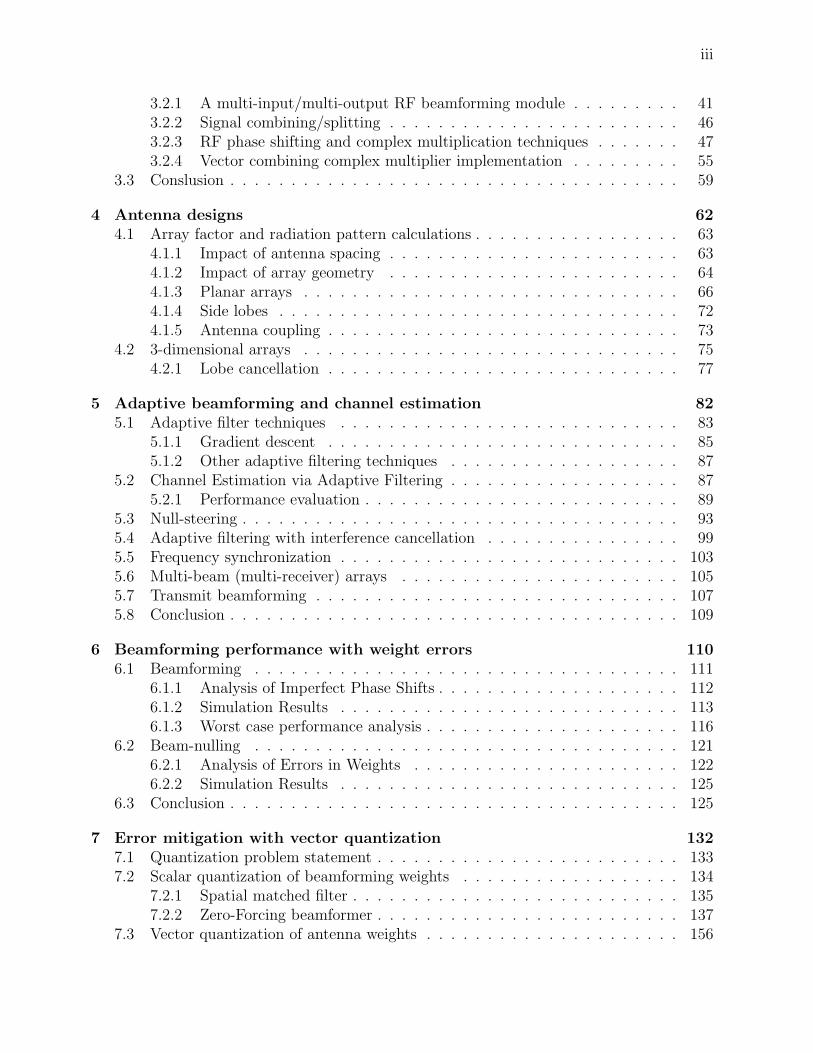
Figure 2.2: Different representations of an antenna pattern in two dimensions: (a) 2D plotin polar coordinates (dB scale) with either θ or φ fixed. (b) 2D plot in polar coordinates(linear scale) with either θ or φ fixed. (c) 2D plot in Cartesian coordinates (dB scale) witheither θ or φ fixed. (d) 2D plot in Cartesian coordinates (linear scale) with either θ or φfixed.

15

1

0.5

0

0.5

1

1 0.5 0 0.5 1 1

0.5

0

0.5

1

1 0.5 0 0.5 1

(a) (b)

1

0.5

0

0.5

1

1 0.5 0 0.5 1 1

0.5

0

0.5

1

1 0.5 0 0.5 1

(c) (d)

1

0.5

0

0.5

1

1 0.5 0 0.5 1 1

0.5

0

0.5

1

1 0.5 0 0.5 1

(e) (f)

Figure 2.3: Three basic patterns (isotropic, omni-directional, directional) in polar coordi-nates (linear scale). (a) Isotropic pattern (azimuth). (b) Isotropic pattern (elevation). (c)Omni-directional pattern (azimuth). (d) Omni-directional pattern (elevation). (e) Direc-tional pattern (azimuth). (f) Directional pattern (elevation). Note that the patterns of theomni-directional and directional antennas depend on the antenna orientation. Here, we as-sume that the omni-directional antenna is oriented such that the radiation is uniform in thexy-plane, and the directional antenna is oriented such that the beam is focused along thex-axis.

16

[54]. In fact, we can write the relationship between the directivity D and the effective areaAe as [60]:

Ae =λ2D

4π(2.2)

where λ is the carrier wavelength. Therefore, for a fixed area, the directivity increases withfrequency.

Beamwidth

Another measure of the directivity is the beamwidth measured near the point(s) on thesphere of peak radiation intensity. There is no fixed definition of the beamwidth. However,the most popular is the half power beamwidth (HPBW), which is the measure of the angleover which the radiation intensity of the antenna is at least one-half the value of its maximumvalue. The directivity is inversely proportional to the beamwidth:

D ∝1

HPBW(2.3)

The constant of proportionality depends on many factors including the size and numberof lobes in the pattern. Also, depending on the context, the HPBW may sometimes referto the solid angle that covers the contiguous area on the unit circle around the peak inwhich the intensity is at least one-half the value of its maximum value. Solid HPBW ispropotional to the product of the azimuth and elevation HPBWs [60]. Other measures ofthe beamwidth include the null to null beamwidth (Bnn) which is a measure of the smallestangle between the peak and the first null (or between two nulls), and the 10dB beamwidth,which measures the angle from the peak up to the point where the intensity drops by morethan 10dB. Equation 2.3 exemplifies the tradeoff of high directivity antennas. Whereas, theenergy efficiency improves with directivity, the coverage area get smaller as well.

2.1.3 Antenna effciency

In all practical cases, antennas are not perfect lossless radiators. In fact, not all the poweraccepted by antenna is actually radiated. The ratio of the radiated power Prad to the poweraccepted or transmitted Pt is radiation efficiency ξ of the antenna. From a transmissionline’s prespective, an antenna is mereley an impedance. The real part of this impedance canbe divided into two components: a radiation resistance Rrad and a loss resistance Rloss. ξcan be expressed in terms of Rrad and Rloss [60]:

ξ =Rrad

Rrad + Rloss

(2.4)

The gain G of the antenna is defined as product of the directivity D and the efficiencyξ. Like the directivity, the gain of an antenna is specified in dBi, which is the ratio of thegain of the antenna to the gain of a lossless isotropic antenna (in dB). Note that the gainof the antenna can be less than 1 even though the directivity is always greater than 1 ifthe efficiency of the antenna bad. The efficiency usually drops at very high frequencies (e.g.mm-wave) where the material loss is high.

17

2.1.4 Antenna bandwidth

From a transmission line’s prospective, an antenna is just an impedance. If not wellmatched, a significant fraction of the transmit/receive power will not be transferred to/fromthe antenna. The bandwidth of the antenna is defined as the size of the frequency bandover which the square magnitude of the reflection coefficient |Γ|2 is smalled than a giventhreshold7. Therefore, in order to ensure maximum power radiation, we need antennas withhigh radiation efficiency and are well matched8.

We note, however, that a lot of the antenna properties like the impedance and radiationpattern can change depending on the medium and the surroundings (especially nearby metalobjects). An antenna that is measured in isolation will usually exhibit slightly differentbehavior when used with an entire system.

2.1.5 Polarization

An electromagnetic (EM) wave cannot be fully described by frequency, phase, and am-plitude since these are scalar quantities. To complete the picture, we also include the polar-ization of the wave, which fully captures its vector nature. In general, radiated EM wavespropagate in spheres. As these spheres become larger, they can be approximated by planewaves over small observation regions. If we fix one of these planes in space, then the figurethat is traced by the electric field vector on this plane with time define the polarization ofthe wave [54]. In general, this figure will be an ellipse, which means that the polarizationcan be fully specified by the orientation of the ellipse and the ratio of the major axis to theminor axis (that ratio is sometimes referred to as the axial ratio or AR). There are, however,some special cases that often occur in practice. When |AR| = ∞, the ellipse becomes a line,and results in linear polarization. On the other hand, when |AR| = 1, the ellipse becomesa circle, and results in either right-hand circular polarization (RHCP) or left-hand circularpolarization (LHCP) depending on the direction of the rotation.

The polarization of an antenna is defined as the polarization of the wave it radiates9. Forexample, dipole and monopole antennas produce linearly polarized waves10. Helix antennasproduce circularly polarized waves (the direction of rotation follows the windings of thehelix). Patch antennas are interesting since their polarization can be controlled by changingthe feed network, so they can be designed to produce any type of polarization [12].

The polarization of an antenna is important in the context of wireless communication fortwo reasons. First, antennas only accept (receive) waves (or components of waves) that havethe same polarization. For example, if an antenna is linearly polarized with a polarizationvector along the x-axis (horizontally polarized), then it will only receive the component(s) ofincoming waves that are polarized along the x-axis. If the incoming wave is linearly polarized

7The threshold is application dependent, but for many applications, an impedance match of -10dB orbetter is considered sufficient.

8For some applications, a narrow band impedance match is desirable to minimize out of band radiation.9The definition is a bit ambiguous since the radiated waves may have different polarizations in different

directions. However, the polarization of the antenna usually refers to the polarization along the main beam[54].

10If the dipole is oriented vertically, then the waves are vertically polarized, and if it is oriented horizontally,then the waves will be horizontally polarized, and so on.

18

with the polarization vector pointing at a direction that is 45 from the x-axis, then onlyhalf the power will be received. Similarly, if the polarization vector is 90 from the x-axis(vertically polarized), then the entire wave will not be received. Using this property, twowireless systems can operate simultaneously on the same frequency band if they each useantennas with orthogonal polarization vectors, which means that in theory we can doublethe capacity by doubling the spectral efficiency by using different polarizations. Therefore,antenna polarization adds an additional degree of freedom to the system. A vertically po-larized antenna is orthogonal to a horizontally polarized antenna, and RHCP antenna isorthogonal to LHCP antenna. Second, in many practical scenarios, the polarization of thewave will impact its propagation through the atmosphere and the reflection coefficients ofdifferent materials. The exact relationship will also be frequency dependent.

In addition to the properties discussed in this section, antenna design is also affected byother factors such as cost and packaging. Some antennas are easier to manufacture thatothers. For example, dipoles and microstrip antennas are easier to print on circuit boardsthan helix or horn antennas.

2.1.6 Free space propagation

Figure 2.4: A transmit antenna Tx and a receive antenna Rx separated by a distance r metersin free space.

Consider a simple example of a transmit antenna Tx and a receive antenna Rx that areseparated by a distance r meters in free space11 as shown in Figure 2.4. If we assume thatthe main beams of both antennas are along the line connecting both antennas, then PRx ,the power received by Rx, is related to PTx , the power radiated by Tx, by the Friis equation[60]:

PRx

PTx

=GTxGRxλ

2

(4πr)2(2.5)

The ratio L = PRx/PTx is called the path loss (the free space path loss in this case). Bydefinition, L ≤ 1. GTx and GRx are the antenna gains of Tx and Rx respectively, and λ isthe carrier wavelength.

11We assume that r is much larger than the dimensions of both antennas.

19

The inverse relationship between the path loss L and the distance r in Equation 2.5 canbe intuitively derived as follows. Since the radiated waves propagate in spheres, at a distancer, the transmit power will be spread over an area that is proportional to a sphere of radiusr. Since the receive antenna has a fixed capture area, the fraction of power captured by thereceive antenna is inversely proportional to the area of the radius r sphere or 1/r2. Equation2.5 can also be written in terms of antenna directivity:

L =PRx

PTx

=ξTxξRxDTxDRxλ

2

(4πr)2(2.6)

The relationship in Equations 2.5 and 2.6 seem to suggest that the free space path loss getsworse as the carrier frequency increases. However, in both equations, we assumed that thedirectivities of both antennas are fixed. If instead, we fix the effective area of each antenna,and rewrite Equation 2.6 in terms of the effective area:

L =PRx

PTx

=ξTxξRxATxARx

(λr)2(2.7)

then the path loss seems to improve as we increase the frequency. There is no contradictionsince we now assume a fixed area instead of a fixed directivity. When the effective area isconstant, then we can get more directivity by increasing the frequency12.

In Equation 2.5, we assumed that the main beams of both Tx and Rx are along the lineconnecting the two antennas, which is not always the case in practice. In order to account forthe misalignment, we multiply the radiation intensities of both Tx and Rx at their respectivepointing angles:

L =GTxGRxFTx(θTx , φTx)FRx(θRx , φRx)λ

2

(4πr)2(2.8)

where (θTx , φTx) represents the direction of the receive antenna with respect to the transmitantenna, and (θRx , φRx) represents the direction of the transmit antenna with respect to thereceive antenna.

Note that the figure of interest is the signal to noise ratio at the receiver or SNR. Thesignal component of SNR (the numerator) is computed from the Friis equation. The noisecomponent (the denomenator) is usually dominated by the thermal noise, which is propor-tional to the absolute temperature T (usually measured in Kelvin) and the signal bandwidthB (usually measured in Hertz). The expression for the noise power (variance) N0 at thereceiver [47]13:

N0 ∼ kTB (2.9)

12In practice, the propagation medium will not be free space, and the loss from medium is usually higherat high frequencies although the relationship is neither linear nor strictly increasing [45]. For example, somebands like 60GHz are very sensitive to oxygen absorption. Thus, the medium loss at 60GHz is going belarger than 80-100GHz even though the frequency is lower. The loss is also affected by other parameters likepolarization.

13Noise is a random process that is modeled as a complex white stationary Gaussian process[47]. Theconstant of proportionality in Equation 2.9 depends on many factors, but most importantly on the receivernoise figure [28]. The constant k in Equation 2.9 is the Boltzmann constant (k = 1.3806503× 10−23m2 · kg ·s−2 · K−1).

20

⇒ SNR ∼ PRx

N0

The capacity C of a link refers to maximum theoretical data rate that can be achieved overthat link, and is bounded by the Shannon limit which is a function of the SNR [47]:

C = B log(1 + SNR) (2.10)

The units for C is bits/sec. C increases linearly with the bandwidth and logarithmicallywith the SNR14. The quantity C/B is known as the spectral efficiency and has units ofbits/sec/Hz.

Equation 2.10 holds for both wired and wireless channels alike as long as the noise iswhite, additive and Gaussian. Channels that have this property are called additive whiteGaussian noise or AWGN channels. For wireless channels however, there is another factorthat needs to be accounted for, which is interference from other sources. In high interferenceenvironments, the quantity of interest is the signal to interference plus noise ratio (SINR).Even though the statistics of interference are usually different from noise, they are oftenassumed to be white and are treated like noise for simplicity15.

2.2 Static versus steerable antennas

The antennas we have discussed so far in this chapter are passive antennas, whose radi-ation characteristics are determined solely by their mechanical structure. Examples includehelix antennas, reflector antennas, and waveguide antennas. The only way to redirect thebeam pattern is by physically moving or rotating the antenna. However, there exists an-other class of active antennas whose properties depend on their electrical characteristics (e.g.impedance, signal excitations) which can be changed to produce different properties withoutaltering the mechanical structure. This class of antennas is sometimes referred to as electri-cally steerable antennas or beamforming antennas or adaptive antennas and is the focus ofthis dissertation.

Electrical beam-steering can be accmplished by means of an antenna array. The simplestexample is a uniform N-element linear array shown in Figure 2.5. The array is uniform inthe sense that all the antennas have the same radiation pattern (typically omni-directional),and the inter-element spacing is the same throughout the array. Suppose for simplicity thatthe array elements lie on the x-axis, and the spacing between two consecutive antennas inmeters is d. Therefore, the total length of the array is Nd. Furthermore, assume that thereis an incoming signal s(t) from an angle θ off the x-axis and a distance r from the firstantenna in the array or (Ant0) as shown is Figure 2.5. We assume for simplicity that s(t)is a very narrow band or single tone signal at frequency f0 corresponding to wavelength λ0

(i.e. s(t) = ej2πf0t = ej2πvst/λ0)16. We also assume that the source of this signal is in thefar field of the antenna array (i.e. r ≫ Nd), so that the received signal at each antenna in

14Note that the SNR itself is a function of the signal bandwidth.15For wireless channels, there is also another statistical factor that impacts the capacity. This factor is

a result of the multipath nature of the channel, and is called fading. Fading is discussed in more detail inSection 2.3.

16vs is the velocity of light in the medium.

21

Figure 2.5: N-element linear antenna array.

the array will have roughly the same amplitude, which we normalize to 1. The same signalarrives at different elements of the array with different delays. Those delays can easily becomputed from the geometry of the array and the angle of arrival and the speed of light inthe medium. Figure 2.5 shows those delays for a uniform linear array as a function of theangle of arrival θ. At a given frequency, these delays translate into phase shifts. If we rotatethe phase of the incoming signal at each antenna Anti by iϑ ∀0≤i<N , then we can derive theexpression of the gain of the array (the aggregated signal from all antennas) as a function ofthe angle of arrival θ and the progressive phase shift ϑ as follows:

relative delay at Antenna i: τi =id cos θ

vs

= iτ ∀0≤i<N

relative phase shift at Antenna i: ϕi = 2πf0τi = 2πi(cos θ)d

λ0

= iϕ ∀0≤i<N

E-field at Antenna i: Ei(t) = ej2πf0(t−τi)+iϑ = ej2πf0teji(ϑ−ϕ)

where τ = d cos(θ)/vs and ϕ = 2πf0τ . We also normalized the delays and the phases suchthat τ0 = ϕ0 = 0. From these expressions, we can calculate the E-field at the output of thearray:

Earray(t) =N−1∑

i=0

Ei(t) = ej2πf0t

N−1∑

i=0

eji(ϑ−ϕ)

∆ , ϑ − ϕ

⇒ Earray(t) = ej2πf0t

N−1∑

i=0

eji∆ = ej2πf0t sin(N ∆2)

sin(∆2)

22

⇒ |Earray(t)|2 =

∣∣∣∣∣sin(N ∆

2)

sin(∆2)

∣∣∣∣∣

2

The term |Earray(t)|2 denotes the increase in the power of the received signal at the output ofthe array relative to power of the received signal at an individual antenna element. However,we also have to account for the noise the output array as well. Since we are adding noisefrom N independent sources17, the noise power at the output of the array scales by a factorof N relative to the noise at a single antenna. Therefore, the boost in SNR at the output ofthe array relative to a single antenna:

SNRout

SNRin

=SNRarray

SNRantenna

=1

N

∣∣∣∣∣sin(N ∆

2)

sin(∆2)

∣∣∣∣∣

2

(2.11)

The ratio of the SNR at the output of the array to SNR at the input of the array (outputof a single antenna) is called the array gain or array factor (AF), which describes how thepower of the radiation pattern varies based on the angle of arrival θ (or angle of departurein the transmit case). The same derivation also applies to a transmit array18. We can seefrom Equation 2.11, the AF is maxmized when ∆ = 0, and the maximum value AFmax = N .That means that the maximum array gain is proportional to the number of antenna elementsand occurs when the signals from each antenna element are all added in-phase19. Figure 2.6shows the normalized array factor of a 20-element uniform linear array with λ/2 inter-elementspacing, with an angle of observation θ = π/6 = 30 from the axis of the array, and ∆ = 0.

Several aspects of the array factor plot, shown in Figure 2.6b, are of interest in a wirelesscommunication system. First and the most obvious is the direction where the beam peaks,usually referred to as the main lobe. The direction of the main lobe is steered towards thedesired target by controlling the phase excitation ϑ. The width of the main lobe is inverselyproportional to the array gain and can be decreased by increasing the effective area of array(by adding more elements without changing the spacing). Second, the other mini-peaks orlocal maximas are called sidelobes. While they may not impact the beam towards the desiredsignal, they can contribute to the overall interference in the system. The level of these sidelobes can be lowered by controlling the relative amplitudes of the signals at the antennas.While the phase is used to steer the direction, the amplitude adds more leverage in shapingthe pattern. In Figure 2.6b, the amplitude is uniform, which results in highest size lobelevels [46]. This is equivalent to multiplying the antenna weights with a rectangular window.However, by “tapering” the window (e.g. using a triangular window), the side lobe levelscan be reduced significantly20. Many techniques used for time-domain filter design apply in

17we assume that the noise is independent across both time and space.18In the receive case, the factor 1/N in AF is a result of adding N independent noise sources. In the

transmit case, the 1/N factor comes from the fact that the transmit power from each antenna is scaled downby N such that the total power transmitted from all antennas is normalized to 1, which is equal to a singleantenna case.

19Since ∆ = 0 is only true for a single frequency, the maximum value of the array factor AFmax = N isonly attained at that frequency. In order to get a wideband response, using a true programmable time delayis necessary.

20Tapering has the effect of reducing the effective area of the array, since using weights that less than the

23

1

0.5

0

0.5

1

1 0.5 0 0.5 1

(a)

-80

-70

-60

-50

-40

-30

-20

-10

0

0 50 100 150 200 250 300 350

(b)

Figure 2.6: Beam pattern of a 20-element linear array with θ = π/6 = 30 and ∆ = 0 (a)2D linear polar plot. (b) 2D rectangular plot. For both plots the elevation angle is fixed atπ/2 (i.e. xy-plane).

24

this context as well [42]21. A more comprehensive discussion on window design, tapering,and side lobe suppression can be found in [12, 46]. Third, the location of minimas or zeros,also called beam nulls, also impact the interference in the system. Beam nulls are usuallysteered towards big jammers. Like the side lobes, null-steering requires controlling both therelative phase and amplitude of the signal at each antenna. Null-steering is discussed inmore detail in Chapters 5, 6, and 7. Finally, notice that the signal also peaks in a directionother than the desired direction θ = 30. This other peak occurs at θ′ = −30, and is calleda grating lobe. The presence of a grating lobe means that signals coming from the directionof the grating lobe have the same relative phase responses at the antennas as the desiredsignal, and are thus indistinguishable. As a result, these grating lobes, which result from thesymmetry in the array geometry, are not desirable22. The grating lobes can be reduced bydesigning the array geometry to break the symmetry. This will be discussed in Chapter 4.

If the antenna elements of the array were all isotropic, then the radiation pattern willbe exactly the array factor. However, the individual antenna elements are not going to beisotropic since such antennas are not realizable in practice. In this case, the overall radiationpattern is the product of the array factor with the pattern of the individual antenna (alsoknown as the element factor or EF) [54]:

F (θ, φ) = AF (θ, φ)EF (θ, φ) (2.12)

where F (θ, φ) is normalized radiation pattern of the array. In practice, mutual couplingbetween neighboring antennas and edge effects make it difficult to have a uniform patternfor all the antenna elements even if those elements were identical. In this case, Equation2.12 will not yield accurate results. However, for large arrays, the edge effects and patterndistortions can be smoothed, in which case, the overall radiation pattern can be approximatedby the product of the array factor with the “average” element factor [54]:

F (θ, φ) = AF (θ, φ)EFav(θ, φ) (2.13)

Although we used a simple example of a uniform linear array to illustrate the basicproperties of phased array antennas, the same concepts and techniques can be used to derivethe properties and radiation patterns of arrays with arbitrary geometries. Some of thesegeometries will be explored in more depth in Chapter 4.

Another advantage of phased array antennas is spatial power combining. On the transmitside, in addition to the increased directivity, the power transmitted by the individual poweramplifiers attached to each antenna are also combined in space. Thus, the signal power atthe receiver is enhanced by a factor of N2 (a factor of N comes from the array gain and

peak weight means that some of the antennas are only partially on. That means that the price of lower sidelobe levels will be a wider main lobe and reduced gain [46]. The shape and level of the side lobes can alsobe changed by changing the geometry of the array.

21The set of complex weights the multiply the signals at each antenna can be viewed as a filter in thespatial domain (similar to the time domain). The corresponding beam pattern can be viewed as the angulardomain representation of the filter (similar to the frequency domain). The relationship between the spatialdomain and angular domain is very similar to the relationship between time domain and the frequencydomain.

22The number of grating lobes also increases when we increase the spacing between the antenna elements,especially when the spacing exceeds λ.

25

another factor of N comes from the spatial power combining). This also means that a singlelarge power amplifier can be replaced by an array of smaller amplifiers that can potentiallybe implemented more efficiently using a low cost silicon technology like CMOS.

The implementation of signal amplitude change and phase rotation as well as signalcombining and splitting is covered in more depth in Chapter 3.

2.2.1 Other types of antenna arrays

Phased array antennas are by far the most popular method for producing a electricallysteerable beam. However, there are other ways of utilizing antenna arrays to steer the beamwithout changing the phase of the signal. These methods include switched array antennasand switched parasitic antennas. Here is a brief overview of each of these methods.

• Switched array antennas

This implementation of beam-steering uses an array of directional antennas (e.g. parabolicdishes) [12]. These antennas can be arranged in a circle for example, with each of thempointing in in a different angle or covering a different sector (the main lobes of the dif-ferent antennas usually have some overlap to ensure continuity of coverage as shownin Figure 2.7). The beam-steering is implemented by turning on the antenna or groupof antennas pointing in the desired direction and turning off the rest of the antennas.The main advantage of switched arrays is simplicity. However, they do not providethe same level/granularity of control over the shape of the beam pattern as do phasedarrays. Furthermore, whereas all antennas in a phased array simultaneously work to-gether to form a beam, only one or a few of the antennas in a switched array effectivelycapture a signal from a given direction. Therefore, in order to provide the same levelof directivity, each antenna in the switched array will have to be as large as the entirephased array. Also, since only a few antennas are used at any given time, the arraydoes not take advantage of spatial power combining to increase the transmit power.

• Switched parasitic antennas

In a switched parasitic antenna, only one of the antennas in the array is excited bya signal; the rest of the antennas around that driven element are parasitic elements[57, 32]. These parasitic elements act like scatterers. The radiation pattern is shapedby changing the electrical characteristics of these scatterers.

Most of the discussion in this dissertation is focused on adaptive antennas based on phasedarrays for the clear advantages they provide. However, many of the ideas and techniquesthat are discussed apply to other beam-steering implementations as well.

2.2.2 Scanning versus adaptive arrays

Beamforming systems can be classified based on their beam shaping capability. For ex-ample, one class of beamforming systems is scanning arrays. As the name suggests, scanningarrays can scan the direction of the beam across a wide range of angles, but do not have theability to create more sophisticated beam patterns with different lobe sizes. However, this ca-pability is sufficient for many applications including radar and line of sight communications.

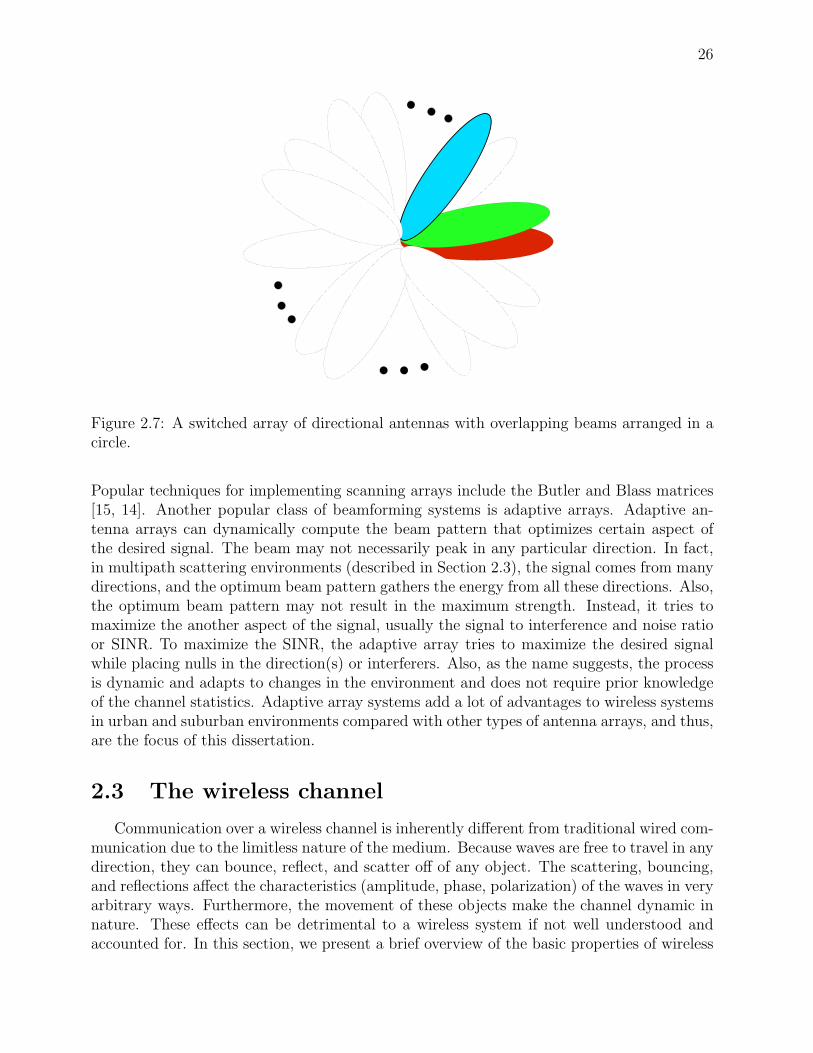
26

Figure 2.7: A switched array of directional antennas with overlapping beams arranged in acircle.

Popular techniques for implementing scanning arrays include the Butler and Blass matrices[15, 14]. Another popular class of beamforming systems is adaptive arrays. Adaptive an-tenna arrays can dynamically compute the beam pattern that optimizes certain aspect ofthe desired signal. The beam may not necessarily peak in any particular direction. In fact,in multipath scattering environments (described in Section 2.3), the signal comes from manydirections, and the optimum beam pattern gathers the energy from all these directions. Also,the optimum beam pattern may not result in the maximum strength. Instead, it tries tomaximize the another aspect of the signal, usually the signal to interference and noise ratioor SINR. To maximize the SINR, the adaptive array tries to maximize the desired signalwhile placing nulls in the direction(s) or interferers. Also, as the name suggests, the processis dynamic and adapts to changes in the environment and does not require prior knowledgeof the channel statistics. Adaptive array systems add a lot of advantages to wireless systemsin urban and suburban environments compared with other types of antenna arrays, and thus,are the focus of this dissertation.

2.3 The wireless channel

Communication over a wireless channel is inherently different from traditional wired com-munication due to the limitless nature of the medium. Because waves are free to travel in anydirection, they can bounce, reflect, and scatter off of any object. The scattering, bouncing,and reflections affect the characteristics (amplitude, phase, polarization) of the waves in veryarbitrary ways. Furthermore, the movement of these objects make the channel dynamic innature. These effects can be detrimental to a wireless system if not well understood andaccounted for. In this section, we present a brief overview of the basic properties of wireless

27

channels and their implications for system design, especially adaptive array systems23.

2.3.1 Channel fading

One of the main consequences of waves bouncing and scattering off of objects is that thesignal usually arrives at the destination from multiple paths. These paths usually have dif-ferent lengths (delays), arrive from different directions (angles), and have different strengths.The statistics of these quantities depend on the environment (e.g. the number and location ofscatterers). In the absence of multipath, the variation in the wireless channel occurs mainlydue to the change in distance between the transmitter and the receiver as these radios movearound. The signal “fades” as the distance between the two radios grows. However, the timescale required for a significant change in the signal amplitude is usually large, and this changewill be largely frequency independent24. On the other hand, when there are multiple paths,the signal can still fade even when the transmitter and receiver are close to each other. Inthis case, fading occurs when the signals from different paths are out of phase at the receiver,which creates a destructive interference. This type of fading has several characteristics thatdistinguish it from the traditional “slow” fading25:

• While the delay from each path is only a function of the length of that path and isindependent of frequency, the phase of the signal is frequency dependent. Therefore,when the signals from different paths are added at the receiver, the magnitude of thesum will also be frequency dependent. Therefore, the fading will be a function offrequency.

• Since any change in the path length that is of the order of the carrier wavelength canrapidly change the phase, any change in the position of the radios or the scatterers thatis of the order of the carrier wavelength can lead to rapid variations in the amplitude ofthe received signal. This is why this type fading is referred to as “small-scale fading”[59].

Therefore, small-scale fading is a function of both frequency and space26. For the rest ofthe dissertation, we shall use the term fading to refer to small-scale fading. A multipathenvironment is usually referred to as a fading environment. Using ray tracing, we canrepresent a wireless channel between two radios in a multipath fading environment in thetime domain with a linear time varying system[59]:

h(τ, t) =∑

i

ai(t)δ(τ − τi(t)) (2.14)

where ai(t) is the amplitude response of path i as a function of time, and τi(t) is the delayof path i (also a function of time). Equation 2.14 describes the wireless channel from the

23The material presented in this section is covered in more detail in [59].24With the exception of the fact that atmospheric attenuation is frequency dependent [45].25In addition to distance, slow or large-scale fading also occurs due to shadowing by large objects like

buildings and hills in non-line of sight environments [59].26Fading can also be a function of time when the some of the radios and/or reflectors are mobile. However,

the temporal variation is a consequence of the spatial variation.

28

transmit antenna to the receive antenna or the wireless channel in RF (passband) domain.However, since most of the processing happens in the baseband, a transfer function thatdescribes the channel from the transmit baseband to the receive baseband would provide alot more insight into the channel characteristics. Recall that the passband signal is an “up-converted” version of the baseband signal (i.e. the passband is obtained by multiplying thebaseband signal by a complex exponential ej2πf0t) [47]. Therefore, in order to convert backto the baseband, we multiply by the complex conjugate (e−j2πf0t), where f0 is the carrierfrequency:

hb(τ, t) =∑

i

ai(t)ej2πf0τi(t)δ(τ − τi(t)) =

∑

i

abi(t)δ(τ − τi(t)) (2.15)

Therefore, the carrier frequency gets canceled. What remains is a phase term ej2πf0τi(t) thatresults from the delay of path i. Equation 2.15 is called the baseband equivalent model [59],and hb(τ, t) is the channel response at the baseband (abi

(t) is the complex response of eachpath at the baseband). Notice that when a path length changes by a quarter wavelength,the phase response rotates by π/2. At 1GHz, a quarter wavelength is a little bit less than8cm. Therefore, the phase response of each path can change rapidly for mobile nodes (onthe order of a few milliseconds).

Most of the wireless systems of interest are digital and have finite resolution limited bythe signal bandwidth Bs (symbol interval Ts ≈ 1/Bs). The relationship between the digital(discrete-time) and analog (continuous-time) signal is:

xb(t) =∑

n

x[n]p(t − nTs) (2.16)

where p(t) is a pulse signal that is band-limited to Bs (e.g. a square pulse or a sinc pulse).When x[n] is replaced by the unit sample δ[n], the discrete-time channel response is obtainedby convolving hb(τ, t) with p(t) and sampling the output at multiples of Ts:

hb(τ, t) ∗ p(t) =∑

i

abip(τ − τi(t))

If we sample at t = mTs, then the lth tap (delay) of the discrete-time channel response is(l = m − n is the discrete-time equivalent of τ):

hl[m] =∑

i

abi(mTs)p(lTs − τ(mTs)) (2.17)

Based on Equation 2.17, if p(t) = Π(t/Ts) (i.e. a square pulse with width Ts), then the firstchannel tap is the sum of paths that arrive in the interval [0, Ts], and the second tap is thesum of paths that arrive in the interval [Ts, 2Ts], and so on (i.e. the lth tap is the sum ofpaths that arrive in the interval [(l − 1)Ts, lTs]).

There are several key parameters (quantities) that are used to capture the basic charac-teristics of a fading environment27. These quantities are statistical in nature, and are usuallyspecified by their root mean square (rms) values. These key parameters are [59]:

27These parameters come in pairs. With each pair describing a certain aspect of the environment incomplementary domains (e.g. time/frequency and spatial/angular domains).

29

• Delay spread: the delay spread Td is the difference in the time of arrival between theshortest path and the longest path [59]28:

Td , maxi,j

|τi(t) − τj(t)| (2.18)

Two factors contribute to high delay spreads: long distance and rich scattering. If theenvironment has a lot of the scattering but short distances (e.g. an indoor environ-ment), then the delay spread will be low (e.g. of the order of tens of nanoseconds).Similarly, if the transmitter and the receiver are far apart, but without any scattering(e.g. line of sight), then the delay spread will also be very low (almost zero). On theother hand, urban and suburban outdoor environments are both long distance and richscattering. In these environments, the delay spread can be of the order of microseconds(sometimes tens of microseconds).

• Coherence bandwidth: the coherence bandwidth Wc is the frequency domain comple-ment to the delay spread and is defined as the size of the frequency band over whichthe channel statistics remain relatively consistent. That means that when part of theband is in deep fade, then with high probability the entire band will also be in deepfade. Two frequencies that are more than a coherence bandwidth apart are assumedto have independent statistics. The coherence bandwidth is the inverse of the delayspread:

Wc ∼1

Td

(2.19)

When the signal bandwidth Bs is smaller than the coherence bandwidth, the channelresponse will be almost flat over the entire signal bandwidth, a situation usually referredto as flat fading [59]. In the time domain, the delay spread will be smaller than thesymbol time Ts, and thus, most significant paths will fall into a single tap (the Fouriertransform of a single tap channel is constant over all frequencies.). On the other hand,when Bs ≫ Wc, the fading will be frequency-selective. In the time domain, Ts ≪ Td,and the channel response will be represented by multiple taps. In our analysis, wefocus on flat fading without loss of generality, since a frequency selective channel canbe transformed into a set of parallel narrow sub-channels, each of them is flat fadingand can be processed independently (see Section 2.3.3).

• Coherence distance: the coherence distance rc is defined as the minimum distance be-tween a constructive interference (channel peak) and destructive interference (channelminimum) [59]. In other words, rc is the minimum distance between two points in spacewhere the channel statistic are independent. The coherence distance not only dependson the environment, but also on the carrier wavelength λ0. This dependence is a resultof the phase (and its rate of change) of each path being a function of the wavelength.Also, depending on the environment, the coherence distance is different in differentdirections. The coherence distance is independent of the delay spread. However, itdepends on another quantity “the angular spread”, which is described next.

28Paths with very low energies are generally neglected.

30

• Angular spread: The angular spread θd is defined as the maximum angle betweentwo paths with significant energy29. Unlike the delay spread, the angular spread doesnot depend on the relative lengths of the different paths, but instead on their angles ofarrival. The angular spread depends on the location of the scatterers/reflectors relativeto the radio. If the radio is located near the scatterers, then the angular spread will belarge, and it will be low when the radio is far away from the scatterers. For example,in an indoor environment, the angular spread is usually high. In an urban outdoorenvironment (a cellular network for example), the angular spread will be high at themobile stations (located near the ground), and low for the base stations (usually ata higher elevation). The angular spread is inversely proportional to the coherencedistance:

rc ∼1

θd

(2.20)

These parameters, together with mobility related parameters, discussed in Section 2.3.1,capture the key features of the propagation environment that help the designers of wirelesssystems improve the overall system design.

Channel variation

The channel variation at fast time scales is mainly due to mobility of the transmitterand/or the receiver as well as, but to a lesser extent, the mobility of the reflectors30. Thecombined effect of the velocity of the radios and the multipath nature of the environmenton the wireless channel can be captured with two complementary parameters:

• Coherence time: the coherence time Tc of a time varying channel refers to the minimumtime required for the statistics of the channel to change. Effectively, the statistics ofchannel change when the wireless node moves a coherence distance away from theoriginal location. That means that the coherence time depends on both the coherencedistance and the velocity of the node(s)31:

Tc ∼vt

rc

(2.21)

where vt is the velocity of the node along the direction of the coherence distance.The coherence time is low in high mobility environments. This situation is usuallyreferred to as fast fading. On the other hand, fixed wireless networks are slow fadingenvironments. Tc is usually of the order of a few milliseconds for fast fading channels.

• Doppler spread: the mobility of a wireless node slightly changes the frequency of thesignal by an amount that is proportional to the ratio of velocity vt of the node to thespeed of the light c:

f ′ = f(1 ± vt/c)

29The angular spread must also specify the direction or the plane of the angle.30Changes in atmospheric conditions (e.g. temperature, air density, rain) also lead channel variations, but

these happen at a much slower scale.31The coherence time depends on the velocity of both the transmitter and the receiver as well as the

reflectors.

31

where the sign depends on the direction in which the node is moving. The changein frequency (∆f = fvt/c) is called a Doppler shift. Since the velocity is going tobe different along different paths (velocity is a vector quantity that is also a functionof direction), the Doppler shift will be different for different paths. Let f ′(i) be thefrequency (Doppler shift) of path i. The the Doppler spread Ds is defined as themaximum in difference in Doppler shift between any pair of paths:

Ds , maxi,j

|f ′(i) − f ′(j)| (2.22)

The Doppler spread is also inversely proportional to the coherence time:

Ds ∼1

Tc

(2.23)

Channel models

We can classify the wireless channel based on the propagation environment into threebroad categories:

• Line of sight

The line of sight or LOS is the simplest model and assumes a single direct path betweenthe transmitter and the receiver. In terrestrial communications, there will be usuallyat least one reflection (e.g. from the ground). Therefore, a perfect LOS channel isunattainable in practice. None the less, LOS is a good approximation to many realchannels. In an LOS channel, fading can be approximated with the Friis equation withan additional exponential factor that captures the loss from the medium32:

L(r, f) =GTxGRxλ

2e−α(f)r

(4πr)2(2.24)

where f is the carrier frequency. The LOS channel is sometimes referred to as theAWGN channel. The delay, angular, and Doppler spreads are zero for an LOS channel.

• Rayleigh fading channel

The Rayleigh channel model is on the opposite extreme of the LOS model. Whereas theLOS model is completely deterministic, the Rayleigh model is completely probabilistic.The Rayleigh model is based on the assumption that each channel tap is sum of theresponses from a large number of independent paths with different lengths [59]. Sincethe lengths of the paths are much larger than the carrier wavelength, it is reasonableto assume that the phase response of each path is uniformly distributed between 0and 2π and is statistically independent across paths. Since there is a large numberof paths, the sum of their complex responses can be approximated with a complex

32The loss exponent is usually dependent on both the medium and the frequency. When the medium isair, the exponential factor in Equation 2.24 is negligible at low frequencies. It becomes significant at highfrequencies. In fact, at frequencies around 60GHz for example, oxygen absorption is a major factor, and theexponential term dominates in long distances [45].

32

Gausssian random variable (using the Central Limit Theorem) [59]. Therefore, thediscrete complex baseband channel taps are modeled as independent complex Gaussianrandom variables. The square magnitude (power) of each of these taps is exponentiallydistributed [59].

The key difference between the Rayleigh fading model and the AWGN model is thatin a Rayleigh model, the channel SNR also becomes statistical. The main consequence

of that the bit error probability (BER) improves as 1/SNR instead of e−SNR as isthe case in AWGN channels [59]. This is one of the major hurdles faced by wirelesssystems.

The Rayleigh channel model is usually adopted for its simplicity. In Chapters 5, 6,and 7, we rely on the Rayleigh channel assumption to simplify the analysis.

• Rician fading channel

In practice, the channel in neither completely deterministic nor completely random.The Rician channel model is used to model channels that lie somewhere between thesetwo extremes (i.e. channels that have a deterministic component and a random compo-nent). The Rician model is effectively a linear combination of the LOS model and theRayleigh. The relative contributions of the deterministic (LOS) and random (Rayleigh)components to the overall channel model is determined by a parameter called the K-factor. A larger K-factor means the channel is more deterministic, and a smallerK-factor means the channel is more random. The K-factor itself is a random variable.The distribution of the magnitude of this random variable is Rician [59].

2.3.2 Channel diversity

The wireless channel response varies in both frequency and space. As we mentionedearlier in this section, the channels become almost statistically independent at locationsthat are more than a coherence distance apart, and frequencies that more than a coherencebandwidth apart. There are different ways for exploiting this property of the channel inorder to improve the channel reliability (i.e. achieve a BER better than 1/SNR):

• By placing multiple receivers (i.e. antennas) or transmitters at multiple locations thatare more than a coherence distance apart, the probability of the channel in all thelocations being in deep fade is reduced considerably. This technique is called spatialdiversity [59]. When implemented at the receiver, it’s called receive diversity, andtransmit diversity when implemented at the transmitter. There are several ways ofcombining the signals from different antennas to obtain diversity. The simplest wayis to choose the strongest channel, and discard all others. This is called diversitycombining. The second method, called maximum ratio combining or MRC33, is littlemore sophisticated, and involves combining all the channels in phase in order to obtainthe power gain in addition to the diversity gain.

Incidentally, spatial diversity is one of the biggest advantages of using antenna arrays.We can also consider this diversity method in the angular domain. The idea is that

33In the signal processing literature, MRC is usually referred to as the matched filter.

33

if the array contains two or more antennas that are more than a coherence distanceapart, in the angular domain, this means that the array has an angular resolution thatis finer than the angular spread of the channel, which means that the array has theability to resolve some paths and significantly attenuate others in order to reduce theprobability of deep fade.

• By communicating over a bandwidth that is larger than the coherence bandwidth,we can reduce the probability of the entire band being in deep fade. This method iscalled frequency diversity [59]. The time domain interpretation of this phenomenonis as follows. When the channel bandwidth is larger than the coherence bandwidth,the symbol time will be smaller than the delay spread. Therefore, the channel willbe composed of multiple taps. Since the statistics of these taps are independent, theprobability of all of them simultaneously being in deep fade is also reduced.

The total diversity in the system will be the product of all these diversity methods.That means if the receiver has NRx antennas that are more than a coherence distance apartfrom each other, and the transmitter has NTx that are at least a coherence distance apartfrom each other34, and the channel has P effective taps in the time domain, then overalldiversity rank of the channel L = NRxNTxP . Diveristy improves the BER from ∼ 1/SNR to∼ 1/SNRL. In the limit as L → ∞, the channel approaches an AWGN channel.

There are other methods for achieving diversity. Time diversity is used in mobile andcellular networks. The idea is that the statistics of the channels change after a coherencetime. So diversity can be achieved by coding and interleaving (spreading) codewords overmultiple coherence times [59]. Time diversity is a product of spatial diversity (radios movingto different points in space). Another method is polarization diversity. With polarizationdiversity, two antennas with opposite polarizations can have independent channel statisticseven when they are less than a coherence distance apart. The reason this is the case is thatwave propagation and reflection are affected by polarization. However, the diversity rankthat can be achieved from polarization is limited since there can only be two orthogonalpolarization states at any given time.

2.3.3 Frequency selective channels

Frequency selective channels improve the system performance by adding more diversity.However, one of the challenges for communicating at the maximum rate over a frequencyselective channel is that since the channel has multiple taps in the time domain, the currentsymbol will interfered with by the delayed versions of previous symbols. This situation isreferred to as inter-symbol interference or ISI [59]. There are several approaches for dealingwith ISI. We describe two of these approaches that are relevant to this dissertation:

• Linear equalization: a linear equalizer is a time domain filter that is chosen such thatwhen convolved with the multitap channel response, the output will be approximatelysingle tap. This method is called equalization because it tries to make the channelresponse equal at all frequencies across the signal bandwidth. The order of the filter

34The coherence distance at the transmitter and the receiver need not be the same. In fact, they areusually different because the angular spreads are different.

34

has to be larger than the channel response in order to get satisfactory results. Whilelinear equalization is not optimal, it provides a good balance between performance andcomplexity.

• Orthogonal Frequency Division Multiplexing (OFDM): this technique transforms asingle wide band channel into a group of narrow band channels, called subcarriers. Thedata are encoded on the subcarriers in the frequency domain, and then converted to thetime domain (using the Inverse Discrete Fourier Transform (IDFT)) to be transmitted.Since each subcarrier is a narrow band signal, the channel response will be flat for singlesubcarrier, but different for different the subcarriers. On the receive side, the receiverconverts the incoming signal back into the frequency domain (using the Discrete FourierTransform) to extract the data off of the subcarriers [59].

Other methods include spread spectrum and optimal maximum likelihood detection usingthe Viterbi algorithm [59].

For beamforming arrays, a frequency selective or ISI means that the single complex weight(amplitude + phase) used at each antenna is no longer optimal. The optimal beamformerwill have to be a complex multitap filter at each antenna. The process of computing theoptimal time domain weights for the filters at each antenna is called space/time adaptiveprocessing or STAP.

2.3.4 Spatial multiplexing

Figure 2.8: A two antenna transmitter antenna Tx communicating with a two antennareceiver in a Rayleigh fading channel.

Consider the scenario shown in Figure 2.8, where a two antenna transmitter is commu-nicating with a two antenna receiver in a Rayleigh channel. Also, assume that the antennason both the transmitter and the receiver are spaced more than a coherence distance apart

35

so that the complex coefficients of the channel matrix H =

[h11 h21

h12 h22

]are statistically

independent (we also assume that the channels are flat fading without loss of generality). Ifthe transmitter transmits data stream x1[n] from the first antenna and x2[n] from the secondantenna, then the received signals y1[n] and y2[n] at the first and second antennas of thereceiver respectively are:

[y1[n]y2[n]

]=

[h11 h21

h12 h22

] [x1[n]x2[n]

]+

[v1[n]v2[n]

]

Or in more compact vector form:

y[n] = Hx[n] + v[n]

where vi[n] is an additive white Gaussian noise signal at antenna i at the receiver. If thereceiver multiplies the input signal y[n] by H−1:

y[n] = H−1y[n] = x[n] + H−1v[n]

then both data steams x1[n] and x2[n] can be recovered at the receiver. This technique iscalled multiple-input/multiple output (MIMO) or spatial multiplexing35, and it is a conse-quence of the Rayleigh fading channel [59]. A prerequisite for spatial multiplexing is thatthe spatial channel matrix H be invertible. In general, the transmitter will have NTx an-tennas and the receiver will have NRx antennas. In this case, the channel matrix H will beNTx ×NRx . The maximum number of independent data streams that can be communicatedsimultaneously over the channel is equal to the rank of H. When the matrix is not square,then the individual streams can be recovered by doing a singular value decomposition on H.The number of “significant” non-zero singular values of H will be approximately the effectiverank of H. If N ′

Tx< NTx is the maximum number of antennas on the transmitter that are

more than a coherence distance apart from each other, and N ′Rx

< NRx is the maximumnumber of antennas on the receiver that are more than a coherence distance apart from eachother, then the effective rank of the channel matrix H is approximately min(N ′

Tx, N ′

Rx).

MIMO and spatial multiplexing are key advantages provided by adaptive arrays for in-creasing system capacity with better spatial reuse. Another easier and more intuitive way tovisualize this problem is through the angular domain. From the angular domain prospective,we can think of the transmitter as encoding different data streams on different paths. If thebeamwidth of the receiver is narrower than the angle separating the paths at the receiver(angular spread), then the receiver array can resolve each path independently. The narrowerthe beams at both the transmitter and the receiver relative to the angular spreads, the moreindependent streams can be transmitter. In general, there is a one-to-one correspondencebetween the spatial and angular domains.

35The antennas do not necessarily have to be attached to the same node.

36

Chapter 3

Radio architectures

The practical implementation of phased-array systems has been greatly aided by recentadvances in silicon technology (especially CMOS), which have made possible the integrationof a large number of radios on a single die. Integrating the components of a multi-antennaradio on a single chip can significantly reduce the overall cost and power consumption of aphased array. However, there are several possible architectures, which each present a differentcombination of benefits and obstacles. The fundamental difference lies in how the signalsfrom the various antennas are combined. In this chapter, we present an overview of threebeamforming architectures (digital, LO, RF), and discuss their advantages and drawbacks.Although we focus on receive side of the system, the same ideas apply to transmit as well.We propose a hybrid RF/digital architecture that combines the benefits of both the RFand digital beamforming architectures in order to meet the overall system capacity and gainrequirements at a much lower cost and power requirement than each of the RF and digitalarchitectures used individually. The chapter is organized as follows. In Section 3.1, weprovide an overview of the three basic architectures, and discuss the pros and cons of each,and describe our proposed RF/digital hybrid architecture. In Section 3.2, we discuss the RFbeamformer implementation.

3.1 Comparison of Architecture

An antenna array must perform two basic operations to dynamically adapt its beampattern: change the phase and amplitude of a signal (i.e. multiplying by a complex numberor providing a programmable complex gain), and add multiple signals from different paths1.This core functionality can be implemented at any stage in the radio transceiver chain (e.g.RF, IF, local oscillator (LO), analog baseband, digital baseband), as shown in Figure 3.1.The different array architectures provide different trade offs among cost, complexity, powerconsumption, and performance. Here, we analyze three of the most popular architectures.

The work presented in this chapter was done in collaboration with Ehsan Adabi and Ali Niknejad[9].

1In the context of transmit beamforming, signal combining is replaced by signal splitting.

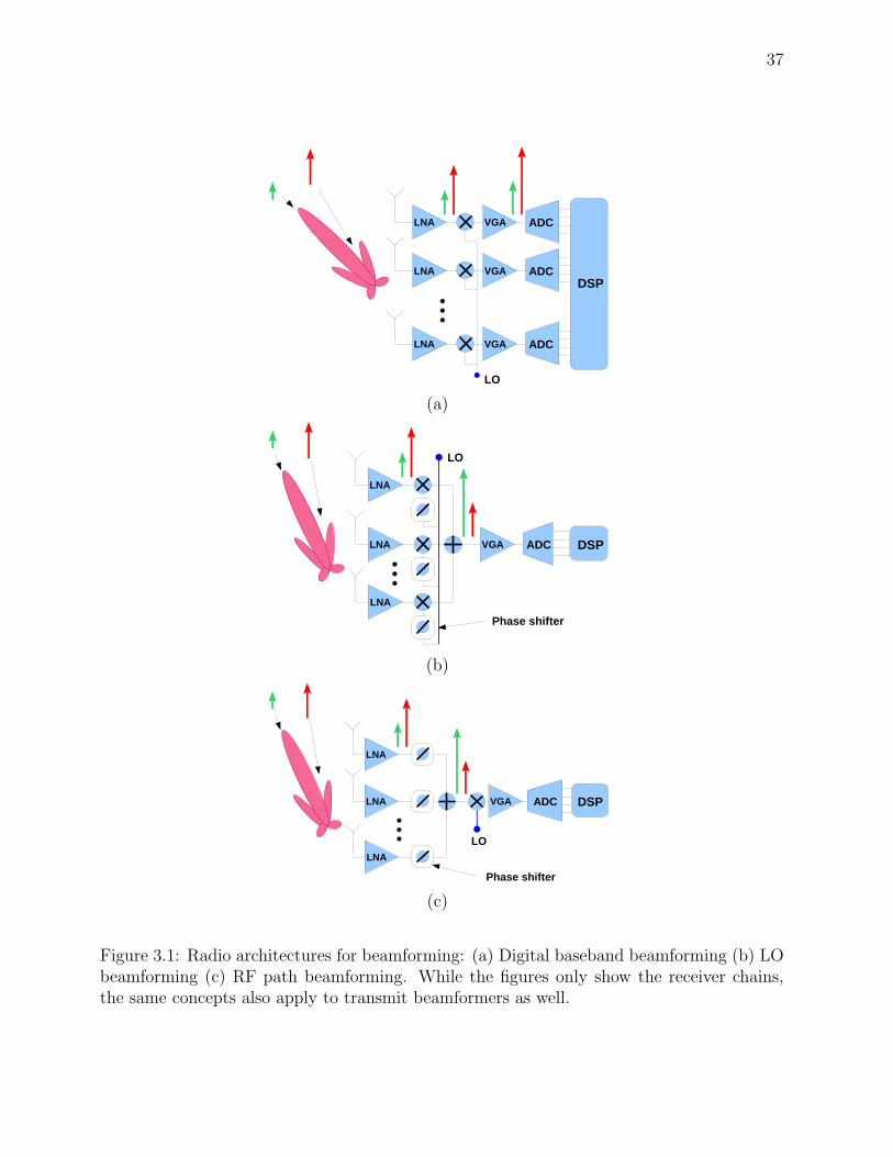
37

(a)

(b)

(c)

Figure 3.1: Radio architectures for beamforming: (a) Digital baseband beamforming (b) LObeamforming (c) RF path beamforming. While the figures only show the receiver chains,the same concepts also apply to transmit beamformers as well.

38

a) Digital baseband beamforming (Figure 3.1a): In this architecture, the core functional-ity is implemented in the digital signal processing domain, after the ADC. Performingthe beamforming functions in the digital domain provides the best performance, sincethe system can exploit high-speed DSPs and implement complex, high-resolution algo-rithms in digital domain. It also makes the system highly flexible, as it is relatively easyto subsequently reprogram the beamforming algorithm. The reconfigurability of thisarchitecture makes it easier to implement wideband, multitap true time delay filters,and thus enables support for multiple data streams in both the spatial and frequencydomains. A technique known as space-time adaptive processing (STAP).

However, there is a price to be paid for this flexibility. First, a digital beamformerrequires a complete transceiver chain per antenna (degree of freedom). This will resultin a significant increase in cost and power consumption, which will in turn limit thescalability (in the number of antennas) of this architecture. The complexity of thedigital baseband processor will also increase in terms of processing power and numberof input/output (I/O) ports. For example, a 20-antenna digital beamformer operatingon a 40MHz signal (sampled at twice Nyquist rate) needs to process 1.6Gsample/sec.If each sample is quantized to 8 bits by the ADC, then this translates to 12.8Gbps tobe processed and at least 20 I/O lines that are 640Mbps each! Second, each of thesetransceivers will have to be tightly synchronized in both time and frequency. Syn-chronization errors especially in frequency can significantly degrade the performance.This tight synchronization is harder to achieve at higher frequencies (e.g. mm-wavebands). At those frequencies, even if all local oscillators (LOs) are to locked to thesame reference clock, the phase noise and jitter can still be significant. Finally, sincethe spatial filtering and interference nulling does not occur until the signal reachesthe digital baseband, all the blocks at the receiver prior to the DSP will have to dealwith the interferers and jammers. Therefore, they should have sufficient linearity anddynamic range to cope with the large blocker levels. This will increase the complexityand power requirements of these blocks. Furthermore, the linearity of the transceiveris not only affected by in band jammers, but also out of band jammers. These, how-ever, can be dealt with using time domain filters with sharp cutoff either at RF or IFand analog baseband. These filters, however, will require a lot of area and sometimesexpensive material (especially if implemented at RF) and thus increase the overall costsince they are replicated for each transceiver.

Multi-input/Multi-output systems, which have become popular in the latest IEEE802.11 and 802.16 standards, are examples of popular systems that are based on digitalbeamforming. However, most practical systems can only support a small number ofantennas or degrees of freedom (typically 4-8).

b) LO frequency beamforming (Figure 3.1b): In this architecture, phase shifting is per-formed in the LO and clock distribution network, while signal combining is performedin IF or analog baseband (depending on the LO frequency). This has the advantage ofreducing the number of ADCs and baseband circuitry, and relaxing the dynamic rangerequirement on them due to spatial filtering after the signal combining. However, thesystem needs a highly symmetric distribution network, to provide the exact desired

39

phase shift, and it also requires significant power consumption in the buffer stages thatare needed to provide a strong LO signal at each of the mixers. In addition, the LO ar-chitecture, like the digital baseband architecture, requires that different signal paths befrequency synchronized. Errors in synchronization can lead to significant performancedegradation. A further limitation is that in general LO phase shifting provides nocontrol over signal amplitudes2. Examples of this architecture can be found in [25, 38]

c) RF path beamforming (Figure 3.1c): In this architecture, both complex multiplicationand signal addition are performed directly in the RF path. The advantages of thisarchitecture are that it provides the lowest component count and power consumption,which yields the lowest cost and best scalability. It also avoids the synchronizationproblem of LO and digital beamforming. However, one drawback is that the designof RF phase shifting components is much more challenging than digital beamformingalgorithms. In addition, the performance is lower than the other architectures, sincepractical phase shifters have non-ideal characteristics (e.g., loss, noise, nonlinearity),which are now directly in the RF path. These problems become even more pronouncedas the frequency increases. Despite the challenges of implementing the beamformingfunctions in the RF domain, this architecture is the best candidate for meeting ourscalability requirements. The implementation of this architecture using integratedcircuit (IC) and printed circuit board (PCB) technology will be discussed in moredetail in Section 3.2.

We also note that while the beamforming is performed in the RF domain under thisarchitecture, the signal processing and parameter optimization can be and is moreefficiently performed in the digital domain. However, the same signal processing tech-niques used under the digital beamforming architecture cannot be reused in this contextsince there is a fundamental difference: the RF beamformer presents the signal pro-cessing unit with only a single input, which is the aggregate signal. The implicationsof this limitation are discussed in more detail in Chapter 5.

3.1.1 Hybrid arrays

We showed in this section that different architectures have their advantages and limita-tions. While it may not possible to meet the system requirements of a particular application(e.g. gain, capacity, cost, power consumption) with one of these architectures, a combinationor hybrid architecture is more likely to achieve those desired features since it will combine thedesired features of multiple architectures. For example, a well designed hybrid RF/digital canachieve high gain and scalability at low cost and power (RF beamforming), and at the sametime achieve high capacity (digital beamforming). Although exact digital/RF breakdown isapplication dependent, here are some general guidelines:

1) The total capacity of the system is proportional to product of the signal bandwidth andthe number of simultaneous spatial streams. The number of simultaneous spatial data

2This can be remedied by using programmable gain blocks in IF or analog baseband prior to combiningthe signals at the receiver, which imposes additional cost and complexity.

40

streams depends on the number of digital I/Os or transceivers3. The bandwidth of theindividual signal also places some limitations of maximum size of an RF subarray. Thesize of the RF subarray has to be such that the maximum difference in time of travelor delay (in any direction between any two elements of the subarray) is small relativeto the symbol duration (inverse of bandwidth). If this condition does not hold, thennot only will the phase shift approximation breakdown, but it may also be difficult toimplement programmable delay blocks at RF that can support these levels of delay.

2) The required rate of adaptation also determines the number of digital I/Os. Since theRF beamformer only has access to the aggregate signal, the RF beamforming weightsare generally slower to adapt than the digital weights. Chapter 5 contains a moredetailed discussion on this topic.

3) The total number of antennas in the array depend on the required gain and steeringrange. If the steering (scanning) range is narrow, then a small number of high gaindirectional antennas can be used. However, when the required scanning angle is wide,then a large number of small antennas need to be used. The number of antennas can beincreased by either increasing the number of RF subarrays or the size of each subarray.The latter option is more cost effective, since it adds more antennas in the RF domainwithout increasing the digital processing and I/Os.

Although the main system requirement that drives the need for more antenna gain isdistance or range, gain is also strongly related to both the capacity and power require-ments of the system since higher gains result in narrower beams that reduce transmitpower requirements and improve the isolation between different spatial streams and arebetter at canceling external interference. Furthermore, the higher gain and improvedisolation increase the reliability of the channel which reduce the probability of errorand enable higher signal constellations that result in better spectral efficiency.

4) The total power consumed is usually dominated by two factors: the RF power amplifiersand the digital baseband processing unit.

Examples of such a hybrid or hierarchical architecture are shown in Figure 3.2. In Figure3.2a, the total area is divided into reticles of subarrays. Within each subarray, beamformingis achieved by RF phase shifting. Then the subarrays are connected and synchronized via thelower clock frequency, and programmed digitally. The beams of each subarray can be uniqueor can be combined with neighboring arrays to create a stronger beam. Multiple targettracking at different directions and different frequency bands will be controlled by the high-speed DSPs that program the subarrays. While this hybrid architecture enables multiplesimultaneous beams, each beam only uses one subarray. Figure 3.2b shows an alternativemultibeam hybdrid architecture that enables each beam to use the entire array. In thisarchitecture, the analog (RF) beamforming architecture is extended to support multiplebeams without significantly increasing the complexity. In order to support K beams, weneed K sets of complex weights. Therefore, the total number of phase shifters or complex

3In theory, the number of digital I/Os has to be at least the number of spatial streams, but is usually alot more in practice.

41

multipliers will increase by a factor of K. The original N × 1 beamformer (where N is thetotal number of antennas) is transformed into an N × K beamformer by replicating thecomplex multipliers and signal adders. If N ≫ K, then we are not significantly increasingthe complexity, because most of the RF components (e.g. PAs, LNAs) are still shared. Underthis architecture, each stream uses the full array.

3.2 RF beamformer design

In Section 3.1, we evaluated multiple architectures for beamforming transceivers. Of thesearchitectures, the one based on RF beamforming is of interest both as a standalone and as afrontend in a Hybrid RF/digital architecture due to its scalability in both power and area.The main challenge of the RF beamformer is implementing the core beamforming function-ality (signal combining/splitting and phase/amplitude correction) in the RF domain. In thissection, we consider the implementation of these blocks in more detail. Before we get intothe circuit details, we first present a high level design of a multi-input/multi-output beam-forming module in RF, and discuss the main requirements that this module needs to satisfyin order to meet the overall system specs. We then present different implementation optionsfor the basic beamforming building blocks and evaluate them in light of those requirements.We note, however, that many of these requirements cannot be perfectly satisfied, and theextent to which they are met is application and frequency dependent4.

3.2.1 A multi-input/multi-output RF beamforming module

Like any conventional antenna, the size of an adaptive array system is also proportionalto the gain and the wavelength. Therefore, silicon integration is not an option for theantennas except at extremely high frequencies (≥ 100GHz). However, the antennas can stillbe printed or mounted on a printed circuit board (PCB) at very low cost. In this case, alarge portion of the cost will be the number of components mounted on the board. Thiscan be reduced by integrating RF blocks from multiple channels (antennas) into a singleIC as shown in Figure 3.3. Figure 3.3 shows a high level block that takes several inputs atRF (from multiple antennas) and outputs multiple linear combinations of these signal (alsoat RF). The linear combinations are programmed through a digital control channel. Figure3.4 shows a chip that supports 16 RF channels mounted on a PCB and feeding monopoleantennas on a ground plane with microstrip lines.

For phased array systems that require antenna gains of 20dBi or more , the number ofantennas can easily be of the order of hundreds. It is almost impossible to support such alarge number in a single silicon chip. However, even it were possible, it is still not a good ideato put that many RF channels on a single chip. First, the traces between the antennas andthe chip will get too long and loss will increase. The advantage of using a small chip is that it

4In this chapter we use the term low frequency to refer to frequency bands with wavelengths that aremuch larger than the size of the module itself. For example, the wavelength at 5GHz is about 6cm, whereas,the area of the entire module may not exceed a few square millimeters. On the other hand, the wavelengthat 60GHz is only a few millimeters and is comparable with size of the chip. However, there really is not anexact cutoff frequency separating the two groups.

42

(a)

(b)

Figure 3.2: Two different architectures for a hybrid (hierarchical) RF/digital beamforming:(a) Large array divided into smaller subarrays connected digitally. Each subarray imple-mented in the RF domain. (b) A single array with multiple parallel RF beamformers. Theoutputs of the RF beamformers are connected and processed digitally.

43

Figure 3.3: Multi-input/multi-output RF frontend.

Figure 3.4: RF beamforming chip with 16 RF I/Os connected to monopole antennas withmicrostrip lines on a PCB.

44

is going to be close to the antennas as shown in Figure 3.4. Second, the cost of the IC dropsin high volumes. If an IC supports 200 channels, it is unlikely to see wide adoption sinceit is very application specific (only applications that require around 200 hundred antennas).However, the advantage of the RFin/RFout chip architecture is that it can be cascaded.We can take advantage of this feature to support antenna arrays of virtually any size. Forexample, suppose we have an IC that supports 16 antennas and outputs 4 different linearcombinations, and we want to build a 64 antenna array. Then we can use 4 of these ICsto connect to 64 antennas, and the output of these ICs is fed to a 5th IC. The four outputsof the 5th IC are then fed to 4 transceivers that convert them into digital basedband to beprocessed by a DSP unit (the reverse is true for transmit).

The multichannel RF IC would integrate the conventional RF blocks (e.g. PAs, LNAs,VGAs, switches) as well as the new beamforming related blocks (e.g. complex multipliersand adders). These components are shown in Figure 3.5a for the receiver and Figure 3.5bfor the transmitter. While both figures show a 4x4 complex vector multiplier block, thenumbers of inputs M = 4 and outputs N = 4 do not have to be restricted (with M ≥ N)5.Figure 3.6 shows these M × N complex modulators as black boxes that take the M input(complex) signals at RF si1, . . . , siM and produce N programmable linear combinations ofthese inputs:

sok =M∑

j=1

cjksij ∀1≤k≤N

where cjk are programmable complex coefficients (gains). The equations can also be writtenmore compactly in matrix form: So = CSi.

The design of these blocks impacts system level performance such as interference rejection.Therefore, there are certain requirements for these blocks in order to meet the system levelspecs. These requirements are:

1) Independent phase and amplitude control must be provided at each signal path. Thisis necessary to give the beamformer tight control over the beam nulls and side lobesto suppress interference.

2) Coupling (cross talk) between different paths must be minimized. That means thatamplitude and phase control on one path should not affect signals on other paths.Coupling impacts the accuracy of beam nulls.

3) The resolution of the phase and amplitude control must be as high as possible, andshould be robust to process and temperature variations.

4) Since all these blocks are in the signal path, the distortion of these blocks must beminimized.

5) The mismatch between transmit and receive paths must be minimized in order tomaintain channel reciprocity.

6) Power consumption and area requirements should be as little as possible.

5The numbers of inputs and outputs are usually chosen as powers of 2 for simplicity.

45

(a)

(b)

Figure 3.5: Building blocks for RF beamforming fronends: (a) Receiver. (b) Transmitter.

Figure 3.6: Multi-input/Multi-output RF complex multiplier block.

46

If we can meet these requirements with a passive implementation, then it is always moredesirable to an active implementation for several reasons. First, a passive implementationdraws a lot less DC power, and is usually a lot more linear. Second and more importantly,passive networks tend to be symmetric (i.e. input/output are interchangeable). That meansthat the same components can be shared among both the transmit and receive chains. Thisnot only reduces the area requirements, but also reduces the possibility of mismatch betweenthe transmit and receive beamformers. However, as will see, it is not always possible to meetall these requirements with passive circuits.

The rest of the chapter covers the implementation of the basic components of the complexmultiplier block in RF: signal combining/splitting and phase amplitude control.

3.2.2 Signal combining/splitting

There are several circuit techniques that can be used for signal combining and splittingat RF. Different choices are appropriate for different frequency bands. For low frequenciessignal combining/splitting is more efficiently done in the current domain [25]. When thisis not possible, power domain combining and splitting is the only option. Popular circuittechniques for power combining use transformers and transmission lines:

1) Transformer-based power combiners: a transformer-based power combiner is shownin Figure 3.7a. It has two desirable characteristics: low loss and compact structure,which makes it appropriate for integrated circuit implementations and a wide rangefor frequency bands. The main disadvantage of the transformer is that it is narrowband. Examples of this type of combiner can be found in [20, 24, 43].

2) Wilkinson power combiners: the Wilkinson is a popular microwave structure for build-ing multi-way power combiners and dividers. A two-way/equal-split Wilkinson divideris shown in Figure 3.7b. The Wilkinson uses quarter-wave transmission line impedancetransformers, and provides three desired properties:

– Simultaneous impedance match at all ports.

– High isolation between combined ports.

– Lossless when all output ports are matched.

Figure 3.11 shows a 2-way/equal-split Wilkinson divider (designed for 2.4GHz) in mi-crostrip printed on an FR4 board. The measurements from this divider are shownin Figures 3.8/3.9. Figure 3.8a shows an insertion loss of about .5dB resulting fromnon-ideal transmission lines. Figures 3.9ab show a low input return loss from all ports.Figure 3.8b, shows a high isolation between the divided ports near the frequency ofinterest. The the isolation and input return loss are wideband when all the ports arematched.

The main disadvantage of the Wilkinson is its size. Since it is proportional to thewavelength, it is more appropriate for high frequencies (e.g. mm-wave or higher),especially for integrated solutions. Furthermore, the insertion loss of the Wilkinson isusually higher than the transformer in practice. Also, it is difficult to implement the

47

Wilkinson network differentially. A more comprehensive analysis of the Wilkinson andother microwave-based power combiners can be found in [45]

Other power combining/splitting networks that combine both transmission lines andtransformer have also been proposed [40].

3.2.3 RF phase shifting and complex multiplication techniques

Several methods have been used to implement a programmable complex gain at radiofrequencies. Here are some examples of these techniques:

1) Extended-resonance/path-sharing phase shifters6: the underlying concept behind thistechnique is a ladder network that evenly distributes the signal across multiple pathswhile at the same time shifting the phase by progressive steps, and thus combiningthe signal splitting and phase shifting functionality into a single network [23]7. Theprogressive phase-shift is usually accomplished by adding a varactor at each stage ofthe ladder to control the shunt impedence. The voltage across the varactor controls theresonance and phase response (the same varactors and the same voltage are used in allstages of the ladder). In addition to combining the signal splitting and phase shiftingfunctionality into a single network, the other advantage of this architecture is that thephases across the elements of the array are controlled by a single parameter (voltage).The network is also passive, which means it can used for both transmit and receivein a time-division duplexing (TDD) system. However, the price of this simplicity isthat the progressive phase distribution is only appropriate for uniform linear arrays.For arrays of arbitrary geometry, the phase-shifts across the different elements will ingeneral not be progressing. Even for linear arrays in a rich scattering environment, thechannel phase responses are unlikely to be progressive. Furthermore, since the arrayrequires a single control parameter, this parameter is required to be high resolution.The required resolution increases logarithmically with the number of antennas in thearray8. Also, a variable control block is required for amplitude tapering if side-lobesuppression is desired9.

2) Reflective-type phase shifters: a reflective-type phase shifter consists of a hybrid 90

coupler, which can be implemented with lumped circuit elements as shown in Figure

6The path-sharing structure can be used with other types of phase-shifters as well. However, extended-resonance has a more compact structure

7The concept of a progressive phase shift is discussed in Section 2.2 in the context of linear arrays.8In Chapters 6 and 7, we analyze the impact of phase and amplitude errors resulting from quantization

and other error sources on the performance of the array. However, in those chapters, we assume that thebeamforming weights are independently chosen for each antenna, and thus the errors can also be assumed tobe independent. This assumption does not hold for this phase-shifting technique since the errors propagate.A more comprehensive analysis of this technique and similar techniques can be found in [41].

9A path-sharing based phase shifting approach is more appropriate in an LO based beamforming archi-tecture. The signal distribution network progressively splits the signal at every junction. At each split, anamplifier is used to compensate for the loss. Unlike, the RF signal, the LO signal is a lot less sensitive tothe gain mismatch at each split especially since it does not require very high linearity.

48

(a)

(b)

(c)

Figure 3.7: Power combining and delay structures: (a) Transformer-based power combiner.(b) Wilkinson power combiner. (c) Discrete programmable delay line implemented withswitched transmission lines.

49

-6.5

-6

-5.5

-5

-4.5

-4

-3.5

-3

-2.5

-2

-1.5

1e+09 1.5e+09 2e+09 2.5e+09 3e+09 3.5e+09

20lo

g|S

12|

frequency (Hz)

Insertion loss S12 of a 2.4GHz 2-way Wilkinson vs frequency

Port 3 matchedPort 3 openPort 3 short

(a)

-25

-20

-15

-10

-5

0

1e+09 1.5e+09 2e+09 2.5e+09 3e+09 3.5e+09

20lo

g|S

23|

frequency (Hz)

Isolation S23 in 2.4GHz 2-way Wilkinson vs frequency

Port 1 matchedPort 1 openPort 1 short

(b)

Figure 3.8: Measured performance of a 2-way Wilkinson power combiner/splitter (printedon an FR4 PCB and designed for 2.4GHz): (a) Insertion loss (S12 = S21) in dB (the idealloss is 3dB resulting from a 2-way power division). (b) Isolation (S23 = S32) in dB betweenthe split ports (the ideal isolation is −∞). In both graphs, the third port was terminatedwith 50Ω.

50

-21

-20

-19

-18

-17

-16

-15

-14

-13

-12

1e+09 1.5e+09 2e+09 2.5e+09 3e+09 3.5e+09

20lo

g|S

11|

frequency (Hz)

Impedance match S11 at combined port of a 2.4GHz 2-way Wilkinson vs frequency

Port 3 matchedPort 3 openPort 3 short

(a)

-16

-14

-12

-10

-8

-6

-4

-2

1e+09 1.5e+09 2e+09 2.5e+09 3e+09 3.5e+09

20lo

g|S

22|

frequency (Hz)

Impedance match S22 at split port of a 2.4GHz 2-way Wilkinson vs frequency

Port 3 matchedPort 3 openPort 3 short

(b)

Figure 3.9: Measured performance of a 2-way Wilkinson power combiner/splitter (printedon an FR4 PCB and designed for 2.4GHz): (a) Input return loss S11 (impedance match) atPort1 (combined port). (b) Input return loss S22 = S33 (impedance match) at Port2/Port3

(split port).

51

3.10 or with tranmission lines, and two reflective loads10. The reflective loads areusually resonant circuits consisting of inductors and varactors. The amount of phaseshift at the output depends on the reflection coefficient ρ = (ZL − Z0)/(ZL + Z0).The phase response is controlled by changing the load impedance. By controlling thevoltage across the varactor, the load impedance can be changed from capacitive toinductive. The range of the phase-shift depends on the range of the varactor. Sincethe load impedance is purely imaginary, the theoretical magnitude of the reflection isalways |ρ| = 1. Therefore, the amplitude response remains constant, regardless of thephase response. Also, since the phase shifter is composed of only passive componentsits both highly linear and symmetric11.

Integrated circuit implementations of this phase-shifter have been demonstrated at ISMbands [63]. However, even a lumped implementation occupies a significant area (usuallydominated by inductors), which is a disadvantage compared to a vector combiningphase rotator described below. Also, a variable gain block after the phase shifter isrequired for tighter control over the shape beam pattern.

Figure 3.10: Reflective-type phase shifter using a hybrid 90 coupler implemented withlumped circuit elements.

3) Programmable delay lines: in wideband applications, the phase-shift approximationno longer holds and a true time delay is required. A simple and straight forward wayto implement a programmable delay is using switched transmission lines as shown inFigure 3.7. Under this structure, the length of the signal path is controlled through theRF switches. If the transmission lines are low loss, then the gain variation across thedifferent delay settings is very small. Since the transmission lines are passive, they canbe used for both transmit and receive12. A discrete 2-bit switched transmission line

10The lumped circuit implementation is more compact than the transmission line implementation, andthus more appropriate for lower frequency bands. The values of the lumped circuit elements depend on thecenter frequency fc and the characteristic impedance Z0 [63].

11The varactor is usually an active component and thus exhibits some non-linearity.12This is true even if the system uses frequency division duplexing or FDD as long as the wireless channel

is a line of sight, since the broadband delay covers both transmit and receive frequency bands.

52

delay implementation on an FR4 PCB for 2.4GHz is shown in Figure 3.11. The maindisadvantage of this technique is that it is very difficult to integrate except at very highfrequencies (e.g. mm-wave frequencies and above). Even for a discrete implementation,every additional control bit requires a pair of RF switches in addition to a transmissionline section. This increases both the cost and the footprint.

A synthesized transmission line is a more compact implementation of a broadbandprogrammable delay and is more suitable for integration [3]. Unlike switched trans-mission lines that use distributed components, synthesized transmission lines can beimplemented with lumped circuit elements that are a lot easier to integrate at lowfrequencies. We note, however, that when the array gets very large, the relative de-lays between array elements on opposite sides of the array are usually much largerthan the maximum delays provided by the programmable delay lines whether they areimplemented with switched or synthesized transmission lines13. In this case, the onlysolution is to divide the array into smaller subarrays such that the maximum delaywithin each subarray is small relative to the symbol duration. Larger delays are betterhandled in the digital domain. Also, this class of controlled delays or phase-shiftersprovide no amplitude control. Amplitude control will require adding a variable gainblock (Section 3.2.4).

4) Vector combining: a fundamentally different technique from the ones listed above inthat it enables simultaneous (in-direct) control of both the signal phase and amplitudeby independently controlling the amplitudes of the real and imaginary components ofthe signal. The basic idea behind this approach is that if we can split the signal intotwo orthogonal components that are 90 apart in phase (e.g. sine and cosine), thenwe can generate any amplitude/phase combination by controlling the amplitudes ofthese two components. The underlying mathematical equations relating the differentquantities:

A cos(ωt) + B sin(ωt) ≡ C cos(ωt + ϕ)

A = C cos(ϕ), B = C sin(ϕ), C =√

A2 + B2, ϕ = arctanB

A

The equations show how the amplitude C and phase ϕ are generated as a function ofthe real Cartesian coefficients A and B. Figure 3.12 shows the general structure of avector combining based complex multiplier. The figure highlights two basic functionsrequired by this architecture, which will be discussed in detail in Section 3.2.4: I/Qsplitting to obtain two orthogonal components (e.g. real and imaginary) of the RFsignal, and amplitude control achieved by a variable (programmable) gain block ateach path in addition to the digital/analog control circuits for programming the gain.Vector combining has several advantages that make it the most appropriate choice foran integrated solution for a wide range of frequency bands. First, it provides reason-ably accurate control over the phase and amplitude of the signal. Second, it can beimplemented with active circuit elements (e.g. transistors) that use very little areacompared to transmission lines or lumped circuit elements like inductors and trans-formers. This feature is very useful for a multichannel implementation that requires

13These delays can span multiple symbol intervals and thus result in intersymbol interference (ISI).

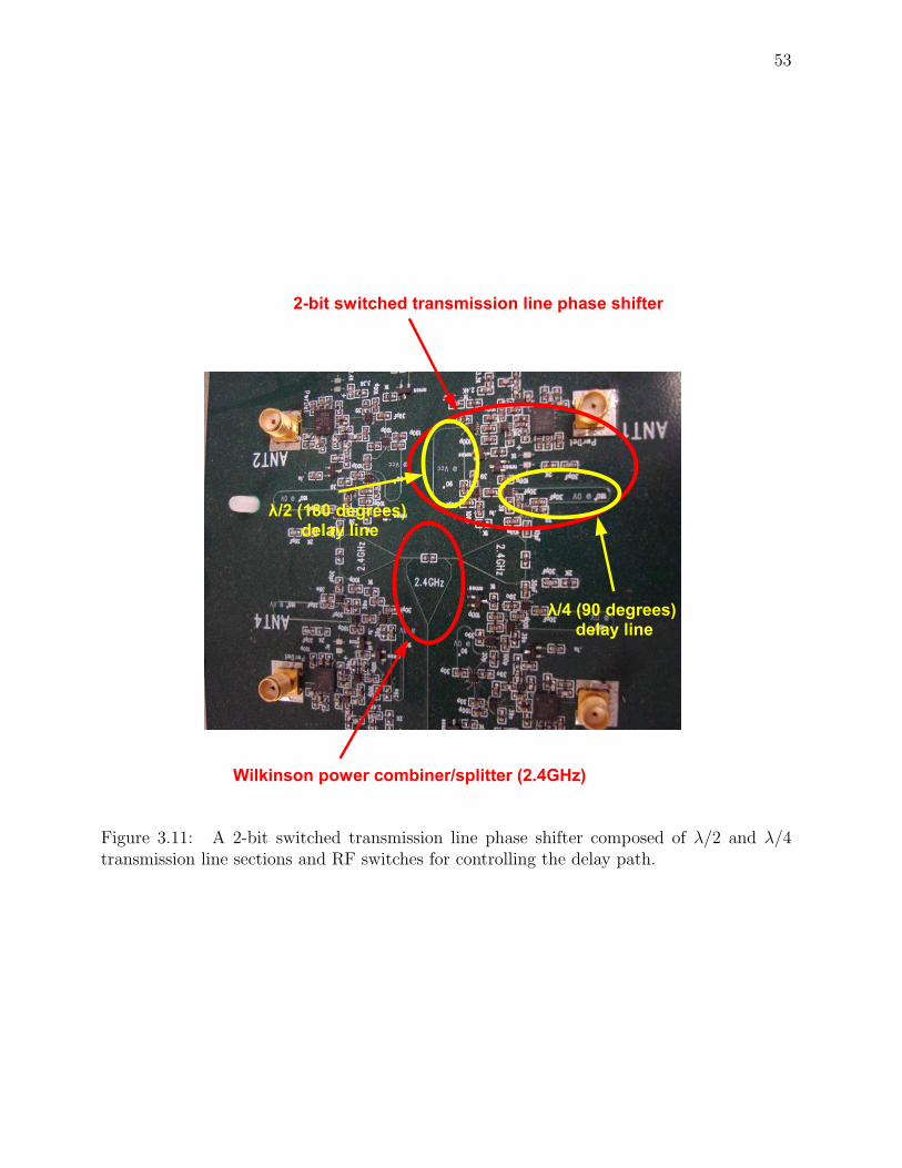
53

Figure 3.11: A 2-bit switched transmission line phase shifter composed of λ/2 and λ/4transmission line sections and RF switches for controlling the delay path.

54

a large number of complex multipliers (Figure 3.2b). Finally, an active/differentialimplementation of the vector combiner can significantly reduce coupling and improvereverse isolation and enable the signals to combined and split in the current domain.

Integrated circuit implementations in CMOS of this scheme have been demonstratedat both lower bands and mm-wave frequencies [43, 5]. While an active implemen-tation is good for reducing area and improving isolation, the price is paid in higherpower consumption, lower linearity, and reduced transmit/receive symmetry (one setof programmable complex gains is required for the transmitter and another for thereceiver)14.

(a)

(b)

Figure 3.12: (a) A digitally controlled complex multiplier (programmable complex gain) inthe RF domain. (b) A 2 × 2 complex multiplier matrix in the RF domain.

14The MOS transistors can be used in triode mode, in which case they behave like passive resistors. Thisimproves linearity, symmetry and power consumption. However, isolation will be a challenge.

55

3.2.4 Vector combining complex multiplier implementation

In this section, we discuss the two main components of a vector combining architecture,namely the I/Q signal generation and the variable gain block.

I/Q signal generation

A Cartesian vector combining based phase rotator requires the signal be split into twoorthogonal components that are 90 degrees apart in phase, usually referred to as the in-phase(I) and quadrature (Q) (or real and imaginary) components of the signal15. There are severalways of obtaining the I/Q components in the RF domain:

1) Polyphase filters: a polyphase filter is a popular technique for splitting an RF signalinto two orthogonal components that are 90 degrees apart in phase. Originally de-signed for image reject mixers, a polyphase filter is a differential passive network ofresistors and capacitors16 shown in Figure 3.13. The outputs at the I and Q portsare 90 degrees apart at all frequencies17. However, the bigger challenge is to get theoutput amplitudes matched since the I path has low-pass characteristic, while theQ path is high-pass. Therefore, the amplitude match occurs at a single frequencyfc = (2πRC)−1. There are several ways to achieve a wideband amplitude match.First, we can cascade multiple stages of the polyphase filter. If resister/capacitor val-ues R1/C1, . . . , RK/CK for K stages are such that their geometric mean is the desiredcenter frequency (fc = ΠK

i=1(2πRiCi)−1/K), then a wideband response can be achieved.

In general, each stage provides an approximately constant gain (within .2dB) within10% of fc. The amplitude response of a 4-stage polyphase filter is shown in Figure3.14. Second, if the system needs to support a narrow band signal over a wide rangeof frequencies, then the gain mismatch can be compensated for using a variable gainblock (described in the next section) or by using variable components in the polyphasefilter itself. For example, if the resistors (or the capacitors) in Figure 3.13 are re-placed by variable resistors (or capacitors)18, then the center frequency can be variedby adjusting the value of these resistors.

The RC polyphase network has several other advantages:

– It’s very compact since it does not contain any inductors, transformers, or dis-tributed elements. Furthermore, the same polyphase network can be sharedamong multiple channels19.

15Orthogonality is not a necessary condition. As long as the components are linearly independent, thenany phase between 0 and 2π can be synthesized in theory by choosing the appropriate coefficients. However,the more orthogonal the components, the more accurate the results are in practice.

16A single ended implementation also exists.17While the actual phase for both I and Q channels varies over frequency, the phase difference is always

90 degrees.18This can be implemented with transistors in triode mode.19The order of the I/Q block and the variable gain block in Figure 3.12 can be interchanged without

affecting the output. Thus, the variable gain block from different paths can be combined before the polyphasefilter

56

– Since the polyphase network is passive, it has a very high linearity and burnsno DC power and is bidirectional. That means that the same network can beshared between the transmitter and the receiver, reducing the transmit/receivemismatch.

– Both the inputs and outputs are in the RF domain. Therefore, it can be used ina cascadable architecture to build larger arrays.

The polyphase network has some disadvantages as well. First, it is very lossy (everystage results in roughly a 6dB loss). Second, it requires a very careful layout toinsure symmetry and minimize the mismatch resulting from parasitics and componentvariation due to temperature and process.

A more comprehensive treatment of polyphase networks can be found in [28, 13].

2) Mixers: another way to produce the I/Q components of the signal is at the output of themixer stage. The advantage of this method is that I/Q components are produced at theLO stage. Although this I/Q generation technique still requires a polyphase filter, a lotthe drawbacks of the polyphase such as loss and amplitude mismatch are avoided sincethey only occur at the LO path20. Therefore, there is little or no amplitude mismatchbetween the I and Q channels at the output of the mixer (except for possible mismatchin the mixer circuit itself as a result of process variation). This scheme, however, hasseveral disadvantages. First, since signal combining occurs post mixing, the mixersmust have high linearity21. Second, the output (combined) signal is no longer in RFdomain. That means that the blocks cannot be cascaded to assemble a larger array22.Finally, this approach is only appropriate in a heterodyne radio architecture [43].

Variable gain blocks

The design of variable gain blocks23 for beamformers and phase-rotating slightly differsfrom conventional VGA design used in automatic gain control circuits (AGCs) in severalways:

1) The phase response of the variable gain block has to be independent of the gain settingespecially at the frequencies of interest.

2) Both the input and output impedances of the variable gain block must also be indepen-dent of the gain setting. A change in the input and output impedances usually impactsthe isolation between different channels and results in phase variation. A simple andstraight forward way to isolate the input and output impedances is by adding buffer

20Since the LO is very narrow band, a single polyphase stage is sufficient. Any amplitude mismatch caneasily be corrected with amplifiers without linearity being an issue since the LO is a “single tone” signal.

21A passive mixer with very high linearity can be used. However, passive mixers a very lossy and thusnegating some of the advantages of this approach.

22An intermediate block or chipset can be designed to take the output signals from each outer RF chip atan intermediate frequency (IF) and add them in the IF domain. However, using this technique requires thatthe LOs feeding the mixers in each of these RF chips to be tightly synchronized.

23We use the term variable gain block to refer to both amplifiers and attenuators. Attenuators maybemore desirable in some applications due to their high linearity and low power consumption [22].

57

(a)

(b)

Figure 3.13: Two equivalent ways of drawing a polyphase filter.

58

Figure 3.14: A wideband 4-stage polyphase network with very good amplitude match.

stages at the input and the output. However, reducing the number of buffer stages isusually more desirable since they affect both the power consumption and the linearity.

3) The gain steps must be uniform and precise.

4) Linearity of the variable gain block is critical since most in-band and out of bandjammers will not be filtered except after the variable gain stage. Furthermore, bet-ter linearity will also improve the accuracy of the gain steps since they will be lessdependent on the amplitude of the input signal.

5) The design of the variable gain block should be robust to temperature and processvariations. Unlike a single antenna system, mismatch between the different channelscan degrade the performance. Therefore, these these variations need to be minimizedor dynamically calibrated. In general, variation and mismatch can be reduced with agood layout, and can be calibrated with a combination of analog and digital techniques.

The linearity and precision are usually improved by using amplifiers with discrete (as opposedto continuous) control steps. For example, many variable gain amplifiers use transistors witha variable (continuous) bias voltage. In this case, the linearity will be very sensitive to thegain setting, and the gain steps are going to be more sensitive to temperature and processvariations. A discrete implementation replaces a single variable-bias transistor with bank ofof switch/fixed-bias transistors as shown in Figure 3.15. Each of the transistors in the bankis hard switched (i.e either set to a fixed bias voltage Vbias or turned off completely). Thegain is controlled by changing the effective size of the virtual transistor represented by thebank (by turning on the right number of transistors). The gain steps will depend on therelative sizes of these small transistors. In order to achieve uniform gain steps and reducethe variation, this concept can be further extended by designing a single unit-gain cell and

59

replicating it as shown in Figure 3.16(a). In this figure, each gain block contains twice thenumber of unit-gain cells as the preceding block. Each block is differential and is controlledby a single bit, which controls the sign of the output. The overall gain is controlled bycontrolling the signs of the sub-blocks. There have been several reported implementationsthat take advantage of this concept [61, 34]. The unit cell in these architectures, shown inFigure 3.16(b), is composed of two differential pairs that are identical except for a sign flip.Only one of these pairs is on at any given time, and the circuit is controlled by differentiallogic. When control bit B = 1, then the current source M1 is turned on (i.e. set to thecorrect bias voltage), and M2 is turned off. In this case, the differential pair M3 and M4 isturned on, and M5 and M6 are off, and vice versa when B = 0. This architecture has severaladvantages. First, the bias current remains constant and independent of the gain setting.This helps reduce the variation of the circuit properties as a function of control signal.Second, the input and output impedances of the variable gain block are also independent ofthe gain configuration. That means better isolation between channels and little or no phasevariation. This also allows the signal splitting and combining to occur in a single stage in thecurrent domain without requiring additional input and output buffers. Since the architectureuses a unit-gain cell, mismatch is also reduced.

In many respects, the design and layout of variable gain blocks for phase shifting are verysimilar to the design of digital to analog converters (DACs).

Figure 3.15: Replacing a single variable-bias transistor with a bank of digitally controlledtransistors. Each of the transistors in the bank are either On or Off (hard switched). Byturning different transistors On and Off, the effective size of the transistor is varied.

3.3 Conslusion

In this chapter, we considered different beamforming architectures and examined theirimpact on the cost, complexity and power requirements of an adaptive array system. Weproposed a hybrid (hierarchical) RF/digital architecture that combines the scalability andpower efficiency of RF beamforming with the speed and flexibility of digital beamforming.The relative sizes of the RF and digital components of the system are determined by thecapacity and gain requirements. We also proposed a multi-input/multi-output RF IC archi-tecture that integrates multiple channels on a single chip and can be cascaded to support largearray with more channels. We examined different techniques and circuits for implementing

60

(a)

(b)

Figure 3.16: (a) A programmable gain block using a unit-gain cell architecture. (b) Unit celltopology.

61

phase shifting and signal combining/splitting. We considered a programmable complex gainblock implementation using a vector combining technique with digitally-controlled variablegain blocks. We showed that this can be a promising architecture for meeting the desiredrequirements of low footprint and accurate phase and amplitude control. Using this tech-nique, signal combining and splitting can be implemented efficiently in the current domainin a single stage. The adaptive signal processing (beamforming) techniques for estimatingand optimizing both the RF and digital beamforming weights are presented in Chapter 5.

62

Chapter 4

Antenna designs

Antenna design is very critical for beamforming systems. Key performance metrics of abeamforming system like range, coverage, and capacity depend very strongly on the antennaproperties discussed in Chapter 2. For example, the range can be extended with higherantenna array directivity, and the coverage (scan angle) can be extended by using arrayswith elements that have wide beams. Capacity is influenced by the antenna in two differentways. First, narrower beams reduce interference and result in better spatial reuse. Second,if the array has polarization diversity (i.e. contains antennas with orthogonal polarizationstates), then this property can also be used to scale capacity even further (by transmittingdifferent data streams on different polarizations) [21]1. Ideally, we would like these quantitiesto be as large as possible. However, the price usually paid is a bigger aperture with a largenumber of elements. The size and form factor are major contributors to the overall cost ofthe system. In Chapter 3, we discussed techniques for designing the radio circuit componentof the beamforming system that can reduce the cost and power consumption of the maincircuit blocks by taking advantage of low cost silicon integration. This chapter focuses onantenna design, with the goal of developing new antenna array design techniques that meetthe system requirements (gain, capacity, coverage) with compact form factors that are easyto build and manufacture at low costs.

The chapter consists of two parts. In the first part, we examine the impact of differentdesign choices (e.g. the structure of the individual antennas and their arrangement withinthe array) on the properties and performance of the array (e.g. gain and radiation patterns).In the second part, we introduce new 3-dimensional array structures and geometries thatachieve the desired results in practice with smaller and more compact form factors compared

The work presented in this chapter was done in collaboration with Ehsan Adabi, Kevin Jones,Jundong Park and Ali Niknejad [9].

1Using polarization for diversity or multiplexing is most beneficial in environments that have little orno spatial diversity (i.e. environments with little scattering like pure line of sight). In environments withrich scattering, there is usually enough spatial diversity to enable independent streams to be transmittedon different antennas with the same polarization. In fact, having different polarizations in a rich scatteringenvironment may not add a significant advantage since the scattering and reflections usually transform thepolarization randomly.

63

with conventional planar antennas. We also present examples that are easy to build andmanufacture using low cost printed circuit board (PCB) technology. In general, reducingthe size of the antenna is more challenging than reducing the size of the radio circuit because,unlike the radio subsystem, the size of the antenna is limited by the laws of electromagneticsand is largely unaffected by technology.

4.1 Array factor and radiation pattern calculations

As discussed in Section 2.1.2, the gain (or directivity) of an antenna is inversely propor-tional to the beamwidth measured in solid angle units2. This gain is also proportional tothe effective area of the antenna. This rule applied to antenna arrays as well.

In Chapter 2, we considered a simple example of a uniform linear array. In this chapter,we generalize the analysis to arrays of arbitrary geometries. To simplify the analysis, wefactor the overall radiation pattern into two components: the array factor and the elementfactor. The array factor (AF) is the pattern of the array when all the antennas are replacedwith isotropic antennas 3. The element factor (EF) is the radiation pattern of a singleantenna element in the array4.

The overall theoretical gain and beam pattern of an array of isotropic antennas dependson three factors: the number of antennas, the spacing between the antennas, and the ar-rangement of the antennas. In this section, we examine the impact of each of these factorson the properties of the beam pattern such as beamwidth, side lobes and grating lobes. Al-though, these different factors are interrelated and it is difficult to quantify each individually,we can still provide some general guidelines on how to take advantage of them in designingthe array.

4.1.1 Impact of antenna spacing

Let N be the number of antennas that are arranged in a linear array (along the y-axis)with equal spacing d between the antennas as shown in Figure 4.2. Let’s also assume thatthe observation angle is along the x-axis (i.e. the array is configured to maximize receptionfrom this angle). When the spacing between the antennas is fixed, then the overall gain ofthe array will be proportional to the number of antennas N (the width of the main lobe willbe inversely proportional to N). On the other hand, if the spacing between the antennas dis increased while number of antennas is fixed, then the gain increases with d up to a point,and remains flat beyond that point. The break point is approximately d ≈ λ/2 (λ is carrierwavelength) [12]. The beamwidth of the main lobe will always be inversely proportional to

2This is often approximated with the 3dB beamwidth (Ω3dB) or 10dB beamwidth (Ω10dB) or the null-to-null beamwidth (ΩNN ). The unit used for solid angles is often called steradians [60].

3Recall from Section 2.1.1 that isotropic antennas have beam patterns that are shaped like spheres (i.e.radiate equally in all directions (azimuth and elevation)) and are represented by dimensionless point sources.An isotropic antenna is an abstract concept and is not realizable in practice.

4We assume for simplicity that the antenna elements of the array are identical. However, this does notguarantee that the beam patterns will be identical. As discussed in Section 2.1.4, the properties of theantenna not only depend on the structure of the antenna itself, but also on the surroundings, especiallythose that are nearby. In Section 4.1.5, we show some simulation results that confirm this observation.

64

d. However, when d > λ/2, grating lobes start to appear. The grating lobes keep the overalldirectivity constant by compensating for the narrowing of the main lobe. These results aredemonstrated in Figure 4.1. In Figure 4.1a, we simulated three uniform linear arrays withdifferent number of antennas (N = 4, 8, 16 respectively) and fixed spacing (d = λ/2) alongthe y-axis with an angle of observation along the x-axis (φ = 0). The figure shows that thewidth of the main lobe being reduced by a factor of 2 for every factor of 2 increase in thenumber of antennas. In Figure 4.1b, we simulated three uniform linear arrays with differentinter-element spacing (d = λ/2, λ, 2λ) and a fixed number of antennas along the y-axis withan angle of observation along the x-axis (φ = 0). The figure shows that the width of the mainlobe being reduced by a factor of 2 for every factor of 2 increase in d. However, the numberof peaks (grating lobes) doubles as well. We also included in Figure 4.1b the beam pattern ofan 8-element linear array with λ/4 spacing in order to illustrate that an increase in spacingcan improve the directivity especially when spacing is small to begin with (i.e. d < λ/2).Figure 4.1b, shows that the 8-element/λ/4-spaced and 4-element/λ/2-spaced linear arrayshave almost identical beam patterns.

4.1.2 Impact of array geometry

A linear array is not a symmetric structure in the sense that it looks different fromdifferent angles of observations. For example, on the one hand, when the array is observedfrom an angle that is orthogonal to the axis of the array, the array appears as a line (i.e.the entire array is observed). On the other hand, when the array is observed from the samedirection as the axis of the array, the array appears as a single point (i.e. only the firstelement is observed). The direction orthogonal to the axis of the array is known as thearray broadside, and the direction along the axis of the array is known as the array endfire(see Figure 4.2). Therefore, it is natural to expect the radiation pattern to be different fordifferent observation angles. For example, consider the two extreme cases (broadside/endfire)plotted in Figure 4.3. Figure 4.3a, shows the azimuth beamwidth much narrower in thebroadside direction than the endfire direction, which may suggest that there is more gain inthe broadside than the endfire. However, gain of the array cannot be based on the azimuthpattern alone; we have to factor in the elevation pattern as well5. Just by looking at thesymmetry of the structure of a linear array, it is easy to see that it provides no elevationgain (i.e. no beam resolution) in the broadside direction6. Similarly, in the endfire direction,the elevation pattern will look identical to the azimuth pattern. Figure 4.3b shows theelevation patterns for both broadside and endfire. Since the overall solid beamwidth canbe approximated with product of the azimuth beamwidth and the elevation beamwidth (i.e.Ω3dB ≈ φ3dBθ3dB), then in order for the gain to be linear in the number of antennas N (inboth cases), we must have the following:

• φ3dB ∝ 1/N for broadside.

• φ3dB ∝ 1/√

N for endfire.

5Recall that the gain is based on the solid angle beamwidth Ω.6The array cannot distinguish signals arriving from different elevation angles in the broadside direction

since they all arrive at the antenna elements with zero relative delay. In fact, the broadside pattern of alinear array is omni-directional (see Section 2.1.1).

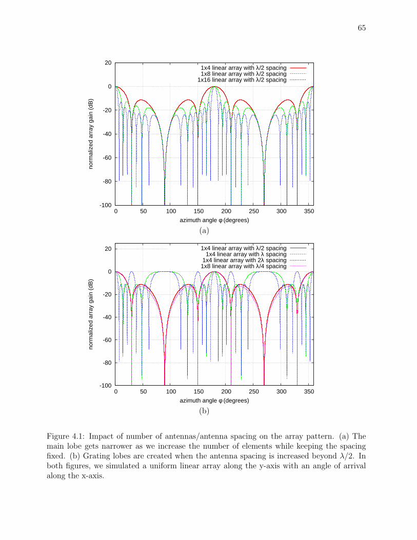
65

-100

-80

-60

-40

-20

0

20

0 50 100 150 200 250 300 350

norm

aliz

ed a

rray

gai

n (d

B)

azimuth angle φ (degrees)

1x4 linear array with λ/2 spacing1x8 linear array with λ/2 spacing

1x16 linear array with λ/2 spacing

(a)

-100

-80

-60

-40

-20

0

20

0 50 100 150 200 250 300 350

norm

aliz

ed a

rray

gai

n (d

B)

azimuth angle φ (degrees)

1x4 linear array with λ/2 spacing1x4 linear array with λ spacing

1x4 linear array with 2λ spacing1x8 linear array with λ/4 spacing

(b)

Figure 4.1: Impact of number of antennas/antenna spacing on the array pattern. (a) Themain lobe gets narrower as we increase the number of elements while keeping the spacingfixed. (b) Grating lobes are created when the antenna spacing is increased beyond λ/2. Inboth figures, we simulated a uniform linear array along the y-axis with an angle of arrivalalong the x-axis.

66

Figure 4.2: Broadside/endfire configurations of a linear array.

In order to verify this, we simulated the endfire and broadside azimuth patterns forN = 10, 100, 1000 in Figures 4.4a (endfire) and 4.4b (broadside) and Table 4.1.2. Theresults clearly show that φ3dB ∝ 1/N for broadside and φ3dB ∝ 1/

√N for endfire. Both

Figures 4.4ab show a 100-element endfire array and a 10-element broadside array havingvery similar beamwidths. In general, angles of arrival that fall in between these two extremecases will behave somewhere in the middle. The azimuth beam pattern of a linear array fordifferent steering vectors (observation angles) is shown in Figure 4.5.

4.1.3 Planar arrays

One of the main disadvantages of linear arrays is their inability to scan the beam in morethan one dimension. For this reason, most practical applications that utilize large phased

67

-120

-100

-80

-60

-40

-20

0

20

0 50 100 150 200 250 300 350

norm

aliz

ed a

rray

gai

n (d

B)

azimuth angle φ (degrees)

64x1 λ/2 spacing (linear array endfire)1x64 λ/2 spacing (linear array broadside)

(a)

-120

-100

-80

-60

-40

-20

0

20

0 50 100 150 200 250 300 350

norm

aliz

ed a

rray

gai

n (d

B)

elevation angle θ (degrees)

64x1 λ/2 spacing (linear array endfire)1x64 λ/2 spacing (linear array broadside)

(b)

Figure 4.3: (c) Impact of the array geometry on the azimuth beamwidth (array steeredtowards φ = 0 (azimuth) and θ = 90 (elevation)). (b) Impact of the array geometry onthe elevation beamwidth (array steered towards φ = 0 (azimuth) and θ = 90 (elevation)).

68

-120

-100

-80

-60

-40

-20

0

20

0 50 100 150 200 250 300 350

norm

aliz

ed a

rray

gai

n (d

B)

azimuth angle φ (degrees)

10x1 λ/2 spacing (linear array endfire)100x1 λ/2 spacing (linear array endfire)

1000x1 λ/2 spacing (linear array endfire)1x10 λ/2 spacing (linear array broadside)

(a)

-120

-100

-80

-60

-40

-20

0

20

0 50 100 150 200 250 300 350

norm

aliz

ed a

rray

gai

n (d

B)

azimuth angle φ (degrees)

1x10 λ/2 spacing (linear array broadside)1x100 λ/2 spacing (linear array broadside)

1x1000 λ/2 spacing (linear array broadside)100x1 λ/2 spacing (linear array endifre)

(b)

Figure 4.4: (a) Azimuth radiation pattern for linear endfire arrays with different number ofantennas. (b) Azimuth radiation pattern for linear broadside arrays with different numberof antennas. In both figures, the arrays are uniform with λ/2 spacing.

69

uniform broadside (λ/2) uniform endfire (λ/2)geometry 1 × 10 1 × 100 1 × 1000 10 × 1 100 × 1 1000 × 1φ3dB 10.02 1 0.1 48.62 15.24 4.8

φ10dB 17.02 1.7 .17 63.2 19.7 6.24

φNN 23.06 2.3 .22 73.8 22.94 7.24

Table 4.1: Simulated azimuth beamwidths of uniform broadside and endfire linear arrays(λ/2 spacing).

-120

-100

-80

-60

-40

-20

0

20

0 50 100 150 200 250 300 350

norm

aliz

ed a

rray

gai

n (d

B)

azimuth angle φ (degrees)

1x16 λ/2 spaced uniform linear array along the y-axis

φmax = 0 degreesφmax = 90 degreesφmax = 45 degreesφmax = 70 degrees

Figure 4.5: Beam pattern of a linear array for different steering vectors.

70

array antennas use arrays with planar geometries. In addition to the ability to scan in everydirection in space, planar arrays have several other advantages7. They have more compactform factors since they pack antennas in two dimensions instead of just one. This allows moreflexibility in choosing the geometry of the array in order to achieve certain beam properties.The compact form factor also improves the bandwidth of phased array systems. Recall thatthe incoming (or outgoing) signal arrives at the elements of the array with different delays.For narrow band (long symbol interval) signals, these delays can be approximated with phaseshifts. However, when these delays become large, this approximation starts to break down.The delays become larger when the array becomes larger (especially between elements atopposite sides of the array). In planar arrays, the maximum amount time required to travelfrom one end of the array to another is going to be much smaller than a linear array ofcomparable gain. Figure 4.6 plots the array factor for different deviations from the centerfrequency for both a 4096-element linear array (Figure 4.6a) and a 4096-element square array(Figure 4.6b). The Figure shows that for the linear array, the gain drops well below 30dBoff the peak when the frequency drifts by 2% from the center frequency. On the other hand,for the square array, the gain is still within 10dB of the peak when the frequency drifts by2%.

Planar arrays do have a drawback, however. Unlike linear arrays, where the array factoris proportional to number of antennas for all observation angles, the array factor of a planararray is not uniform. In general, the gain of a planar array is larger in the broadside direction(direction orthogonal to the plane of the array) than in endfire directions (directions on thesame plane as the array elements)8. In order to demonstrate this, we simulate the endfireazimuth pattern of an M ×N rectangular array on the xy-plane (M is the dimension alongthe x-axis or the depth of the array, and N is the dimension along the y-axis) with an angleof arrival along the x-axis (i.e. φ = 0, θ = π/2). We fixed N = 10 and varied the depth of thearray M from 1−400 to see the impact on the azimuth beam pattern. The plots are shown inFigure 4.7. The figure shows little improvement in the width of the main lobe as we increasethe depth of the array from 1 to 400. In fact, the main lobe starts decreasing only whenM > 100. The planar array is behaving like a linear endfire array of linear broadside arrays.Since the azimuth endfire beamwidth is proportional to 1/

√M and broadside beamwidth

is proportional to 1/N , the broadside pattern dominates when N >√

M , and the endfirepattern dominates when M <

√M . Therefore, the azimuth endfire beamwidth φ3dB of a

rectangular array is proportional to min(1/N, 1/√

M) instead of 1/(N√

M)9.

7In a real system, the scanning range will be limited by the antenna elements. However, in this sectionour focus in on the array factor.

8Recall that the gain (or directivity) of an antenna is proportional to its effective area. The effective areaof a planar array is larger in the broadside direction than in the endfire direction.

9That means that total gain in the endfire direction will be proportional to N√

M (or M√

N dependingon the direction of arrival). The extra factor of

√M comes from the elevation gain. On the other hand, the

overall broadside gain of a planar array is NM (N is the azimuth gain and M is the elevation gain) [12].Therefore, the different between the broadside and endfire gains is a factor of

√N or

√M . Although the

plots in Figure 4.7 show that the side lobe levels decrease significantly as the depth of the array increases,the gain from side lobe reduction diminishes very quickly and cannot make up for the

√M lost gain.

71

-80

-70

-60

-50

-40

-30

-20

-10

0

10

20

30

40

54 54.5 55 55.5 56

norm

aliz

ed a

rray

gai

n (d

B)

azimuth angle φ (degrees)

4096x1 uniform linear array with λ/2 spacing

∆f = 0∆f = 0.02fc∆f = 0.04fc∆f = 0.06fc∆f = 0.08fc

∆f = 0.1fc

(a)

-80

-70

-60

-50

-40

-30

-20

-10

0

10

20

30

40

50 52 54 56 58 60

norm

aliz

ed a

rray

gai

n (d

B)

azimuth angle φ (degrees)

64x64 uniform square array with λ/2 spacing

∆f = 0∆f = 0.02fc∆f = 0.04fc∆f = 0.06fc∆f = 0.08fc

∆f = 0.1fc

(b)

Figure 4.6: (a) Array factor of a 4096-element uniform linear array with λ/2 spacing fordifferent deviations from the center frequency (fc). (b) Array factor of a 4096-elementuniform square array with λ/2 spacing for different deviations from the center frequency(fc).

72

-120

-100

-80

-60

-40

-20

0

20

0 50 100 150 200 250 300 350

norm

aliz

ed a

rray

gai

n (d

B)

azimuth angle φ (degrees)

1x10 λ/210x10 λ/2

100x10 λ/2200x10 λ/2400x10 λ/2

Figure 4.7: Azimuth endfire pattern of rectangular arrays. Different curves corresponds todifferent array depths M .

4.1.4 Side lobes

Any radiation outside the main lobe of the beam is usually undesirable because is createsunnecessary interference. In a well designed antenna, most of the radiation outside themain lobe comes from side lobes that are weaker than the main lobe10. However, for someapplications, even the side lobe radiation levels are unacceptable. So far in our analysis, wehave assumed that the antennas are excited with equal amplitudes. This will lead to thehighest directivity because the entire array aperture is fully utilized [12]. Unfortunately, thispattern of excitation also leads to the higher side lobe levels. If we look back at patternplots for linear arrays and planar arrays (e.g. Figures 4.3 and 4.4), we see that althoughthe width of the first side lobe becomes narrower as we increase the size of the array, itsamplitude relative to the main lobe remains constant (approximate -13dB below the mainlobe) [12]. There are two ways to control the side lobes levels. The first way is by controllingthe amplitude of the signal excitation. As we mentioned in Section 2.2, whereas controllingthe relative phases of the signal excitations helps steer (direct) the beam, controlling therelative amplitudes of the signal excitations helps shape the beam. For a uniform lineararray, choosing the relative amplitudes to reduce the side lobe levels is very similar to thewell known problem of designing a digital/time domain finite impulse response (FIR) filter,and lot of the techniques for designing time domain filters apply to spatial domain filters

10As we have seen earlier, radiation can also come from grating lobes which are comparable to the mainlobe. However, grating lobes are a lot easier to avoid than side lobes as will be shown in Section 4.2. Gratinglobes can also be filtered out by the element pattern.

73

as well [42, 12]. The second way to reduce the side lobe levels, which is less obvious, is byproperly designing the geometry of the array11. To get an idea how the side lobe levels areaffected by the array geometry, consider the pattern plots of a square array shown in Figure4.8. The figure shows the pattern of a 10 × 10 square array antenna for two observationangle φ = 0, 45. The figure clearly shows that when the beam is steered towards a 45

azimuth angle, then the side lobe levels are lower than when it is steered towards the x-axis. The reason is that the shape of the array looks different from a 45 angle. Section 4.2discusses some techniques for designing the array geometry to minimize side lobes. Note thatregardless of the technique used (e.g. controlling amplitude and/or geometry), the reductionin side lobe levels usually comes at the price of reduced directivity [12].

-120

-100

-80

-60

-40

-20

0

20

0 50 100 150 200 250 300 350

norm

aliz

ed a

rray

gai

n (d

B)

azimuth angle φ (degrees)

10x10 λ/2 spaced uniform square array

φmax = 0 degreesφmax = 45 degrees

Figure 4.8: Side lobe level for different angles of arrival.

4.1.5 Antenna coupling

In the preceding sections, we focused our analysis on the array factor. In this section, weconsider the impact of the array geometry on the element factor. The design and properties ofthe antenna element are critical because they determine the coverage and polarization stateof the system. In Section 4.1.1, we showed that the minimum spacing d between antennas inthe array required to achieve the maximum theoretical array gain is dmin = λ/2. In practice,however, the required dmin maybe larger than λ/2. Real antenna elements have physicaldimensions and are not dimensionless point sources, and thus, the presence of neighboring

11This mostly applies to planar arrays.

74

Figure 4.9: (a) 3-dimensional radiation pattern of an isolated dipole. (b) 3-dimensionalradiation pattern of a diplole in a circular array with λ/2 spacing.

antennas creates coupling that distorts the radiation pattern (usually results in a net loss),and alters the impedance of the antenna (affects the bandwidth). Naturally, the couplinggoes down as the spacing between the antenna elements increases.

Figure 4.9a shows the radiation pattern of an isolated dipole, and Figure 4.9b, shows thedistortion in the pattern after placing the dipole in a circular array with λ/2 spacing. As aresult, the realized beamforming gain is usually less than what is predicted by theory (the losscan be as large as 2-3dB). The loss will also depend on the angle of arrival since the distortionis not uniform. The distortion will also depend on the type and polarization of the antennasbeing used (e.g. patches, monopoles, dipoles), since different types will be affected differentlyby different array geometries [12]. In some cases, the distortion in the beam pattern mightresult in some antennas having increased gain in some directions relative to others. Sincethese directions are usually different for different antennas in the array (different antennassee different surroundings), these non-idealities in the beam patterns might average out in alarge array and the total gain will be comparable to the case of a uniform array. However, inthis case, we do not get the full benefit of spatial power combining since a significant portionof the array might not be radiating efficiently in a given direction.

In order to show the impact of antenna spacing on coupling and pattern distortion, wesimulated the peak beamforming gain (accounts for both the element factor and the arrayfactor) of different uniform square arrays (with different antenna spacings) of monopoleantennas with finite ground plane in HFSS [1]12. The results are shown in Table 4.2. Whenwe increase the size of the array from 3 × 3 to 5 × 5, the expected theoretical gain wouldbe 10 log(25/9) ≈ 4.4dB. However, the simulation results show that increasing the numberof antennas from 3 × 3 to 5 × 5 by reducing the spacing from λ to λ/2 yields only 1.8dBadditional gain. While increasing the number of antennas by reducing the spacing from2λ to λ yields 4.3dB additional gain (almost the entire predicted gain). This means that

12The finite ground plane also contributes to the loss in symmetry of antenna patterns.

75

spacing λ/2 λ 2λgeometry3 × 3 – 10.2dB 10.3dB5 × 5 12dB 14.5dB –

Table 4.2: Simulated array gain versus the spacing between antennas.

increasing the spacing from λ to 2λ does not improve the coupling situation by much, whichmeans that in this case λ spacing provides a good trade off between gain and coupling13.

Although the increase in spacing necessary to avoid coupling might give rise to gratinglobes, in practice, several of these lobes will be filtered (attenuated) by the beam patternof individual antennas. For those that are not, we present an array topology in Section 4.2for canceling or significantly attenuating them. We note, however, that even though λ/2spacing may not yield the expected (theoretical) beamforming gain, there are other benefitsto having more antennas such as increased diversity and transmit power (by having moreradiating elements).

4.2 3-dimensional arrays

In Section 4.1, we looked at how different design choices (number of antennas, spacing,array geometry) influence the radiation pattern and gain of the array. In this section, wepropose a new class of array structures that utilize all 3-dimensions, and analyze them inlight of the constraints discussed in Section 4.1. As we mentioned earlier, the goal is toachieve as much directivity, coverage (in both azimuth and elevation), and diversity (in bothspace and polarization) as possible. In this context, using 3-dimensional arrays may seem likean obvious choice given that they use space a lot more efficiently. However, the advantagesof using a 3-dimensional array structure are a little more subtle than that. Recall that thedirectivity of an antenna array (or any antenna) is proportional to the surface area. weshowed in Figure 4.7 that increasing the depth on array does not to lead narrower beams.Also, 3-dimensional structures are generally more difficult to build and manufacture. Thismight lead us to conclude that using 3D array adds little or no value to the system. However,the advantages of using 3D arrays become clear after further examination:

• We showed in Section 4.1.3 that the array factor of a planar area is not uniform in alldirections since the effective area is larger in some directions (broadside) than others.On the other hand, when all three dimensions are used (e.g. a cubic array), the arraygeometry and the gain become more uniform in all directions.

• Although increasing the depth of the array does not improve the width of the mainlobe, it can reduce the side lobe levels significantly. Also, as we will demonstrate laterin this section, the depth of the array can be exploited to cancel grating lobes that

13The optimal spacing will depend on the geometry and radiation patterns of the individual antennas.

76

arise from large spacing between elements of the array. This property can significantlyimprove the beam shaping capability of the array.

• Since more antennas can be packed in a three dimensional structure than a planarstructure, the aggregate transmit power (spatial power combining) can be increasedwithout increasing the transmit power of individual power amplifiers. Furthermore,having more antennas, while not necessarily contributing to the overall directivity ofarray, provides better redundancy and reliability. If one antennas fails, then there areseveral backups.

• A larger number of antennas also leads to better noise averaging. Although the direc-tivity of an array is proportional to the number of antennas on the surface N2, whereN is the number of antennas (length) in each dimension, there is a total of N3 receivingantennas. The background noise picked up by those antennas will not be completelyuncorrelated14, and thus, the signal to background noise ratio at the output of the arraywill not improve beyond N2. However, the thermal noise generated by the receiverswill be independent across different elements, and thus, the component of the noise atthe output of the array that is due to thermal noise can be reduced by N3 relative tothe desired signal. In most systems, the thermal noise dominates over the backgroundnoise15. Therefore, a 3-dimensional array receiver can improve the overall noise figureof the system16.

• Since we can pack a larger number of antennas in the same amount of space, and notevery antenna contributes equally to the gain, we can design different antennas withdifferent properties in order to achieve pattern and polarization diversity. Since it isdifficult to achieve all desired properties (e.g. coverage, polarization) with a single typeof antenna elements, using a mixture of different types is the only viable solution inpractice.

Figures 4.10 and 4.11 show examples of 3-dimensional arrays. Figure 4.10 shows a cubicarray composed of multiple stacked planar arrays (sheets). Each sheet is a square array ofmonopole antennas. Figure 4.11 shows a similar array with a cylindrical shape. In additionto having a more compact form factor than planar arrays and conventional static directionalantennas, the arrays shown in Figures 4.10 and 4.11 have other advantages as well:

• In these array designs, our choice for an antenna element was a monopole antennawith a ground plane. We chose monopoles because they are easy to manufactureand assemble, and have an omni-direction pattern, which enables beam steering in

14Antennas pickup noise from the environment. The noise temperature of the background noise dependson the angle of arrival [45]. The correlation of the background noise picked up by different antennas in thearray depend on many factors including directivity.

15The contribution of the thermal noise to the overall noise at the output of a receiver is captured by thenoise figure (NF). The noise figure is defined as the ratio of the SNR at the input of the radio to the SNRat the output of the radio [28].

16Depending on the number of antennas, this property can be utilized in different ways. For example, ifwe relax the noise figure requirements of a receiver, we might be able to design the amplifiers with less poweror better linearity. However, this is still an open problem that requires further investigation.

77

any direction in the azimuth plane17. Furthermore, since monopoles do not radiatevertically, the presence of a ground plane (a wavelength away) from above has little orno effect on their beam patterns.

• Each sheet can be realized with a printed circuit board (PCB), and the presence of ametal ground plane simplifies the process of mounting the digital and analog electroniccomponents. The feedlines for the antennas can be implemented using microstrip lineson the PCB, which significantly reduces the cost of manufacturing and assembly. Theloss from microstrip lines is not an issue since the amplifiers (e.g. PAs and LNAs) canbe placed very close to the antennas.

• The different sheets (PCBs) can be connected with one another by mounting them onanother PCB.

• Compared with array structure shown in Figure 4.12 (a sectorized array of patchantennas), which also provides the desired 360 coverage and can be configured tohave polarization diversity, the 3D arrays in Figures 4.10 and 4.11 can be built toimprove on the transmit power and noise figures of the system18.

4.2.1 Lobe cancellation

Increasing the antenna spacings beyond λ/2 has other undesirable effects beyond theincrease in size. The most important one is the creation of multiple main lobes, also knownas grating lobes, most of which will point towards undesired directions [12]. These gratinglobes appear in the theoretical array factor of the antenna. In fact, even a linear array withλ/2 spacing exhibit grating (back) lobes in both the broadside and the endfire directionsbecause of the symmetry, with the number of grating lobes increasing as we increase thespacing. One way to break the symmetry and eliminate or reduce the size of grating lobes intheory is to reduce the spacing between the antennas to λ/4. Figure 4.1 shows the theoreticalarray patterns of two uniform square arrays with the same area but different spacings: λ/2and λ/4. In Figure 4.14a, with both array patterns configured to point towards 90o, we seethat the λ/2 spacing has a back lobe pointing towards 270o that gets reduced by almost25dB when the spacing is λ/4. In Figure 4.14b, we see that when both arrays are pointingtowards 45o, the back lobes for both spacings are at a significantly lower power level thanthe main lobe. The reason for this is that looking through the diagonal of the array, thespacing between the antennas is no longer λ/2, but

√2

2λ instead, which automatically breaks

the symmetry since√

22

λ ≈ 34λ. However, in both figures we notice the level of side lobes

17Ideally, we would like to be able steer the beam in any direction in space. Unfortunately, isotropicantennas are not realizable in practice. However, if complete coverage is required, it can be achieved with amixture of antennas in the array such that their “aggregate” pattern covers the entire space. For example,we can put patch antennas on the top and bottom sheets in Figures 4.10, 4.11 in order to cover the verticaldirections. Also, we can utilize other types of antenna that are easy to print on a PCB and provide adifferent polarization from the monopole. Another way of achieving different polarizations is by changingthe orientation of some sheets relative to others.

18In the patch array, since only a few sectors are pointing at the desired direction at any given time, thetransmit power from other sectors is not fully utilized.

78

Figure 4.10: 3-dimensional rectangular array of monopoles.

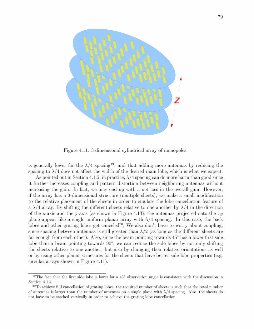
79

Figure 4.11: 3-dimensional cylindrical array of monopoles.

is generally lower for the λ/4 spacing19, and that adding more antennas by reducing thespacing to λ/4 does not affect the width of the desired main lobe, which is what we expect.

As pointed out in Section 4.1.5, in practice, λ/4 spacing can do more harm than good sinceit further increases coupling and pattern distortion between neighboring antennas withoutincreasing the gain. In fact, we may end up with a net loss in the overall gain. However,if the array has a 3-dimensional structure (multiple sheets), we make a small modificationto the relative placement of the sheets in order to emulate the lobe cancellation feature ofa λ/4 array. By shifting the different sheets relative to one another by λ/4 in the directionof the x-axis and the y-axis (as shown in Figure 4.13), the antennas projected onto the xyplane appear like a single uniform planar array with λ/4 spacing. In this case, the backlobes and other grating lobes get canceled20, We also don’t have to worry about coupling,since spacing between antennas is still greater than λ/2 (as long as the different sheets arefar enough from each other). Also, since the beam pointing towards 45 has a lower first sidelobe than a beam pointing towards 90, we can reduce the side lobes by not only shiftingthe sheets relative to one another, but also by changing their relative orientations as wellor by using other planar structures for the sheets that have better side lobe properties (e.g.circular arrays shown in Figure 4.11).

19The fact that the first side lobe is lower for a 45 observation angle is consistent with the discussion inSection 4.1.4

20To achieve full cancellation of grating lobes, the required number of sheets is such that the total numberof antennas is larger than the number of antennas on a single plane with λ/4 spacing. Also, the sheets donot have to be stacked vertically in order to achieve the grating lobe cancellation.

80

Figure 4.12: Planar and sectorized patch arrays (8 sectors).

Figure 4.13: A multi-sheet/3-dimensional rectangular array of monopoles with λ/4 shifting.

81

-100

-80

-60

-40

-20

0

0 50 100 150 200 250 300 350

norm

aliz

ed a

rray

gai

n (d

B)

angle (degrees)

15x15 λ/4 spacing8x8 λ/2 spacing

(a)

-100

-80

-60

-40

-20

0

0 50 100 150 200 250 300 350

norm

aliz

ed a

rray

gai

n (d

B)

angle (degrees)

15x15 λ/4 spacing8x8 λ/2 spacing

(b)

Figure 4.14: Comparing the theoretical array patterns (in the azimuth (xy) plane) of twouniform square arrays with same area, but different spacings (λ/2 and λ/4). (a) Both arrayssteered to towards 90. (b) Both arrays steered to towards 45.

82

Chapter 5

Adaptive beamforming and channelestimation

At a high level, a multi-antenna receiver maximizes the SNR by steering its main beamtoward the desired signal and nulling out any interfering signals. If the receiver knows thechannels responses of the various transmitters, then the problem becomes trivial. In practice,though, the channels from the various transmitters are unknown a priori, and will vary intime. Thus, the system must be able to adaptively estimate the channels and compute theoptimum beamforming weights. Designing optimal methods1 to accomplish this task, alsoknown as adaptive array processing techniques, is heavily influenced by the radio architectureof the array and its hardware capabilities. Most of the previous work in this area has focusedon the digital beamforming architecture, while the RF beamforming architecture has receivedvery little attention.

The fundamental difference between the digital baseband and RF architectures that im-pacts beamforming is that the digital architecture offers access to the input signals fromeach individual antenna element in the array (prior to combining), whereas the RF architec-ture only offers access to the aggregated signal(s)2. Thus, in a pure digital architecture, thesignals from each antenna are digitized and stored. This capability enables the signals tomanipulated and combined in multiple ways. That means that the optimum beamformingweight vector(s) can be computed and updated while data is being received. Furthermore,multiple spatial data streams can be extracted simultaneously. On the other hand, the RFarchitecture enables only a single way to aggregate the signals at any given time. This meansthat amount of time and training samples required to estimate the optimum beamformingweights is much larger than the digital architecture, which creates an additional overhead

The work presented in this chapter was done in collaboration with Mark Johnson, RaghuramanMudumbai, Kannan Ramchandran and Ben Wild [11, 10, 8, 9].

1The performance criteria will vary from system to system system. These include speed, accuracy, andcomplexity. There is usually a trade off between these factors, and the optimal combination will depend onthe system requirements.

2Multi-beam and hybrid RF/digital architectures discussed in Chapter 3 can have M > 1 differentaggregated outputs. In general, however, M ≪ N , where N is the number of antennas.

83

since it is difficult update the weights while data is received3. This makes most beamformingtechniques developed for the digital architecture unsuitable for the RF beamforming archi-tecture. Therefore, new beamforming techniques need to be designed that are tailored forthe RF architecture, which is the focus of this chapter.

Most of the previous work on beamforming schemes that rely only the aggregate signalat the output of the array were based on greedy energy maximization [36, 37]. In [36], ascalable algorithm that utilized a single bit feedback was proposed. The algorithm proceedsby adding small random perturbations to the beamforming weights at each step. If the newweights result in a higher SNR at the output of the array, then the new weights are retained.Otherwise, they are discarded. It was shown that if the magnitude of the perturbationsis small enough, then the algorithm is guaranteed to converge, and the number of stepsrequired grows linearly with the number of antennas N . However, the main disadvantage ofthis class of algorithms is that they are slow to converge and are very sensitive to noise andinterference4. Also, while the convergence time scales linearly with the number of antennas,the constant factor is usually too large for most practical systems.

In this chapter, we present a more flexible and robust framework for computing thecomplex beamforming weights based on adaptive adaptive filtering. The chapter is organizedas follows. In Section 5.1, we present a brief overview of popular adaptive filter techniques.In Section 5.2, we show how to use these techniques to estimate the optimum beamformingweights. The problem of null-steering and the null-steering performance are discussed inSection 5.3. In Section 5.4, we consider the problem of beamforming in the presence ofinterference. In Section 5.5, we discuss the problem of frequency synchronization and fastfading channels and show how the adaptive filter framework can be modified to handlefast changing channels and large frequency offsets. We discuss multichannel and hybridRF/digital architectures in Section 5.6. Finally in Section 5.7, we conclude with a briefdiscussion on transmit beamforming.

5.1 Adaptive filter techniques

Statistical channel estimation and filter design and optimization occur in a wide varietyof applications. Although different applications have different requirements, a lot of theseproblems share a common structure and can be written as:

wHx[n] = d[n]

x[n] = [x[n], x[n − 1], . . . , x[n − K + 1]]⊤

where x[n] is a complex column vector (sequence) of order K of data at time n, d[n] is acomplex scalar denoting the desired (training) signal at time n, and w denotes a discretetime complex order K linear filter5. The interpretation of the data and the desired signal are

3The size of this overhead depends on the rate of channel variation as well as the system requirements.4It is difficult to reliably detect energy levels even in moderate SNR regimes.5In this chapter, we denote scalars in lower case, vectors in bold lower case, and matrices in bold upper

case.

84

application dependent6. However, the goal is to find the linear combination7 of data samplesthat best approximates the desired signal at time n. In practice, the “best” or optimumsolution is defined in terms of the minimum mean square error (MMSE) criterion:

e[n] = d[n] − wHx[n]

wMMSE = argminwE[‖e[n]‖2]

This solution is obtained by solving the Normal Equations (sometime refered to as theWeiner-Hopf equations) [50]:

wMMSE = R−1xx rdx (5.1)

Rxx = E[x[n]x[n]H ], rdx = E[d[n]Hx[n]]

Rxx is the K × K autocorrelation matrix of x[n], and rdx is K × 1 cross-correlation vectorof the desired signal d[n] and x[n] (the data vector)8. The solution in Equation 5.1 isalso referred to as the Weiner or least squares solution. This solution is derived from theorthogonality principle, which states that the power of the error signal is minimized whenthe error signal is orthogonal (uncorrelated) with the data9:

E[e[n]x[m]] = E[(d[n] − wHMMSEx[n])x[m]] = 0 ∀n,m

⇒ E[d[n]x[m]] − E[wHMMSEx[n]x[m]] = 0 ⇒ rdx[n − m] = wHrxx[n − m]

⇒ rdx[k] = wHrxx[k]

where rxx is the kth column of Rxx. To solve for the K coefficients of wMMSE we need Kequations (i.e. k = 0, . . . , K−1), which is equivalent to Equation 5.1. In general, the secondorder statistics Rxx and rdx are not known a priori, and are usually estimated from sampleaverages (Rxx and rdx are used instead of Rxx and rdx). In practice, however, the normalequations are not usually solved by directly inverting the Rxx (or Rxx) for several reasons:

1) The data sequence x[n] is not available all at once, but instead is received over time.Therefore, waiting for the entire sequence to be available may introduce unnecessarydelay.

2) The data set x[n] maybe too large that computing and inverting Rxx maybe com-putationally unfeasible.

3) The statistics of the signal x[n] are usually not known a priori and frequently varywith time, and thus using the entire data set to compute the optimum weights vector(filter) may lead to inaccurate results.

6In communication systems, the desired signal is usually a known pilot signal defined by the system apriori.

7In this chapter, we focus on finite impulse response filters (FIR). We will also assume that all signalshave zero means (i.e. E[x[n]] = E[d[n]] = 0).

8We assume that these second order statistics are stationary. Otherwise, we need to include the timeindex (e.g. Rxx[n], rdx[n]).

9The results are simplified by assuming that x[n] and d[n] are wide sense stationary and jointly widesense stationary signal, which means that their first and second order statistics are independent of time [47].

85

This motivated the design of a class of filters, known as adaptive filters, that addressesthese issues. Adaptive filters have the following properties:

1) The computation of the beamforming weights proceeds on a sample by sample basis.That is the filter taps are incrementally updated when a new sample (or a group ofsamples) is received, as opposed waiting for the entire sequence. This is sometimesreferred to as online versus batch mode computation. This property addresses thelatency problem.

2) The computational complexity of updating the filter taps when new samples are re-ceived is far less than direct matrix inversion. This addresses the complexity problem.

3) The algorithms do not assume any prior knowledge of the signal statistics.

4) More recent samples have stronger influence on the values of the filter taps than oldersamples. This, together with Properties (1) and (3), gives the algorithm the ability totrack changes in the signal statistics, and is what makes those filters truly adaptive.

Figure 5.1 shows the basic structure and building blocks that most adaptive filters havein common. Adaptive filters are closed loop systems. The error signal (or a function of it)in the feedback loop is used to update the filter taps. Different adaptive filters have differentupdate equations, which in turn depend on the error criterion and other factors.

5.1.1 Gradient descent

One of the most popular classes of adaptive filters are based on the concept of Gradientdescent. Gradient descent defines how the filter taps get updated in order to minimize someerror criterion ξ. The filter taps update proceeds as follows:

gn+1 = gn − µ∇gnξn (5.2)

where gn is the vector of filter taps at time (iteration) n, ∇gnξn is the gradient of the error

criterion ξn with respect to the filter taps gn, and µ is the step size (a scalar that determinesthe rate of adaptation and convergence). Since the gradient defines the direction of themaximum rate of change, the error is minimized by moving in the opposite direction of thegradient (and hence the name gradient descent). One of the most popular error criteria isthe mean square error (MSE). The generic minimum mean square error gradient descentproblem is shown in Figure 5.1. The goal is to select the filter taps such that the outputof the filter, when the input is the random sequence w[n], is as close as possible to thedesired sequence d[n] in the mean square sense. The MSE is defined as follows:

ξn = E[|e[n]|2] where e[n] = d[n] − gTnwn (5.3)

⇒ ∇gnξn = ∇gn

E[e[n]e∗[n]]

= ∇gnE[(d[n] − gT

nwn)(d∗[n] − gH

nw∗

n)] = −E[e[n]w∗

n]

86

Figure 5.1: The standard MMSE adaptive filtering problem.

⇒ gn+1 = gn − µ∇gnξn = gn + µE[e[n]w∗

n] (5.4)

The difficulty in applying gradient descent directly lies in the fact that computing theexpectation in Equation 5.4 requires prior knowledge of the first and second order statisticsof the signals, which defeats the purpose of using a “blind” algorithm. Therefore, in mostimplementations, expected values are replaced by sample averages. By far the simplest andmost popular implementation is the LMS, which replaces the expected values of randomvariables with their instantaneous values 10, and works well in practice. The LMS updateequations are as follows:

desired sequence: d[n], input sequence: w[n]

l-tap FIR filter: gn = [gn[0], gn[1], . . . , gn[l − 1]]T

wn = [w[n], w[n + 1], . . . , w[n + l − 1]]T , error sequence: e[n] = d[n] − gTnwn

Filter update: gn+1 ← gn + µe[n]w∗

n(5.5)

The following condition is sufficient to guarantee that the filter taps converge (in the meansquare sense):

µ ≤ 1

trRww[n]where Rww[n] =E[wnwH

n] is the autocorrelation matrix (of order l ) of the random sequence

w[n] (which can potentially be time varying). In general, a smaller value of µ leads tobetter convergence, while a larger value leads to faster adaptation and better tracking, butcan make the algorithm less stabe11. The convergence time τ of the LMS algorithm isroughly:

τ ∼ 1

µ

λmax

λmin

(5.6)

10This is why it is sometimes referred to as the “stochastic” gradient descent algorithm.11The value of µ doesn’t have to be fixed, and can be varied as a function of time (µn) to achieve a better

compromise between convergence and adaptation.

87

where λmax and λmin are the largest and smallest eigenvalue of Rww respectively. Theadaptive filter can be initialized to any random value (usually the filter taps are set to 0)without affecting the asymptotic convergence time of the algorithm.

The LMS algorithm works very well in practice and is very widely used in communicationsystems for channel estimation and equalization. One of the reasons the LMS is very popularis its low computational complexity. The number of operations required to update the filtertaps is proportional to the number of taps (i.e. O(l)). There are several variants of theLMS algorithm that optimize some aspect of the performance like stability (e.g. NormalizedLMS) or computational efficiency (e.g. sign-LMS)12.

5.1.2 Other adaptive filtering techniques

There are other adaptive filters that are widely used that are not based on gradientdescent. The most popular example is recursive least squares (RLS). RLS usually leads tomuch faster and more accurate convergence than LMS, and does not depend on the eigenvaluespread as is the case with LMS. However, this improvement in speed comes at the price ofextra compuational complexity (the number of operations required for each update step isquadratic in the number of filter taps ( O(l2))).

Even though both LMS and RLS do not require any prior knowledge of the signal statis-tics, they both require a reference (training) signal (e.g. d[n]) that is known a priori13.There is another class of adaptive algorithms that do not rely on a known reference signal,but instead adapt based on some property of the data signal (e.g. constant modulus). Suchalgorithms are usually much slower to converge, and are not always guaranteed to convergeto the correct result.

A more comprehensive treatment of adaptive filters can be found in [50, 27, 26].

5.2 Channel Estimation via Adaptive Filtering

System identification is one of the classical applications or formulations of the adaptivefilter problem. The general system identification problem is illustrated in Figure 5.2. Thealgorithm generates a random (usually white) sequence w[n] that is fed into the system withunknown impulse response h or transfer function H(z) (H(z) is the z-transform of h)14. aswell as to an adaptive filter gn (transfer function Gn(z))15. that is used to approximate the

12In the standard LMS algorithm, the size of the update to the vector gn in Equation 5.5 will be directlyproportional to the magnitude of the data (regression) vector x∗[n]. This can have some undesired effects onthe performance of LMS. Normalized LMS avoids this problem by dividing the step size µ by |x[n]|2 at eachstep. Sign-LMS or sign-error LMS on the other hand, simplifies the required computation in the update stepby quantizing the real and imaginary parts of the error signal e[n] to a single bit (the sign bit). However,the saving in computation comes at the expense of slower convergence [50].

13The reference signal can sometimes be predicted from the data itself. For example, in a communicationsystem, after a signal is decoded, the output of the decoder can used to train the adaptive filter. Such atechnique is called decision-based or decision-directed adaptive filtering. However, even in such cases, theLMS or RLS algorithm still needs to be initialized (boot-strapped) using a reference (pilot) signal that isknown a priori. This pilot needs to be injected at regular intervals in order to avoid instability.

14We assume that the unknown system is linear.15Sometimes we denote a filter with a subscript n (e.g. gn) when the filter taps are time varying.

88

Figure 5.2: Identifying the impulse response of an unknown system using adaptive filtering

unknown system. The output from the unknown system is used as the desired signal d[n]:

d[n] = (h ∗ w)[n]

e[n] = d[n] + ν[n] − (gn ∗ w)[n]

(h ∗ w)[n] ,

∞∑

k=−∞h[k]w[n − k]

where ν[n] is noise signal (usually white) that models the noise in the system, and (∗) denotesthe discrete convolution operator. It is clear from the equations above that the variance ofthe error signal is minimized when g → h as n → ∞ (e[n] is reduced to white noise sequence).

The unknown system response does not necessarily have to be a time-domain filter. Infact, in the case of beamforming, the unknown system to be identified is a spatial filter.The algorithm proceeds in a similar manner. For example, a receiver Rx estimating thecomplex channel response at each antenna from a remote transmitter Tx using the systemidentification framework would follow these steps16:

0) Rx locally generates a random sequence w[n] (making the samples of w[n] i.i.dusually results in faster convergence)17.

1) Tx sends a known pilot x[n]. The choice of x[n] does not matter much since the samesignal is received at the different antennas at the receiver. Furthermore, we assumethat if the transmitter has multiple antennas, the transmit beamforming weight vectorremains fixed throughout this process.

16Without loss of generality, we assume that the channels are narrow band or single tap (flat fading)channels. A large delay spread (frequency selective) channel can be converted into a group of smaller narrowband subchannels (e.g. OFDM), where the complex channel response is flat fading.

17w[n] can be sampled from any distribution (e.g. Gaussian, Bernoulli, etc.). The choice will dependon several factors such the set of available beamforming weights, which determines both resolution and thedynamic range. For example, when the beamformers have low resolution, a Bernoulli distribution maybepreferable since it takes only two values (e.g. 1, -1). However, as we show in Section 5.4, using thisadaptive filtering based framework in the presence of interference will require much higher resolution for thebeamforming weights. We note, however, that the accuracy of channel estimation does not depend on theresolution of the beamforming weights, but instead depends on the resolution of the A/D component.

89

2) Rx sets the antenna weights (beamforming weight vector) to a block of length N(number of antennas) of the random sequence w[n].

3) At each time step n, the block of w[n] assigned to the antenna weights is shifted tothe right by one sample. Thus the output of the array at the receiver y[n] mimics thetime domain covolution of the sequence w[n] with an N tap filter (channel responseh)18.

4) The received signal at the output of the array y[n] = wH [n]h[n]x[n] + ν[n] is usedby the adaptive filter as the desired signal (y[n] is the output from the A/D afteraggregation). The error signal e[n] is used to update the N tap filter gn.

These steps are summarized in Figure 5.3. The figure shows how the channel vector froma transmitter to a multi-antenna receiver can be estimated by posing the problem in thesystem identification framework. The complex vector h is the unknown channel responsefrom the transmitter to each antenna in the array19. The adaptive filter can be implementedby one of the standard algorithms (e.g. LMS or RLS). When the step size in the filter ischosen appropriately, the filter coefficients g[n] will approximate h, the unknown channel20.Observe that while the beamforming weights may be applied in the RF or analog domains,the computation of those weights occurs in the digital domain.

5.2.1 Performance evaluation

In this Section, we analyze the performance (both speed and accuracy) of the adaptivefiltering based beamformer. We also consider the impact of noise and channel variation. Forsimplicity, we will focus on the Normalized LMS (NLMS) algorithm. However, the resultsextend to a generic adaptive filter.

Let us begin by deriving the expression for the running time under NLMS. Recall fromEquation 5.6 in Section 5.1.1, the convergence time of the LMS algorithm τ :

τ =1

µ

λmax

λmin

Since the elements of the sequence w[n] are chosen i.i.d:

Rww ∼ Rww = σ2wIN

⇒ λmax

λmin

≈ 1

18It is not strictly necessary for a spatial filter to simulate a time domain filter. For example, new setsof N weights can be generated independently at each time step n and the subsequent algorithm will stillrobustly estimate the channel. In fact, we show in Section 5.4 that in order to cancel a known interferer,emulating a time domain convolution may no longer be an option.

19In a rich-scattering multipath environment, the channel responses usually follow a Rayleigh distribu-tion (i.e. the channel coefficients are i.i.d. complex Gaussian random variables). In a clear line of sightenvironment, the channel coefficients are functions of the array geometry and the direction of arrival.

20because y[n] is a noisy version of the true desired signal d[n] (due to the presence of the white (thermal)noise signal ν[n]), gn will be a close, not an exact, estimate of h

90

Figure 5.3: The transmitter sends a known signal, and the multi-antenna receiver employsan adaptive filter to estimate the optimal beamforming weights.

91

where σ2w = E[w[n]∗w[n]] (for simplicity we choose σ2

w = 1), and IN is the identity matrix ofsize N . The step size µ under NLMS is chosen as:

µNLMS =µ

′

ǫ + ‖w[n]‖2

where µ′

is a constant (usually µ′

< 1) that is independent of the regression data w[n], w[n]is a vector of size N of the regression data at time n, ǫ is a positive number to avoid divisionby zero or by a small number when ‖w[n]‖2 is close to zero21. Since E[‖w[n]‖2] = σ2

wN = N :

µNLMS ∼ 1

N

⇒ τNLMS ∼ 1

µNLMS

= O(N)

Therefore, the number of steps required for convergence is proportional to the number ofantennas N . This result is not surprising. Another more intuitive way to think about this isthat since we are solving for the N coefficients of unknown spatial filter, we require at leastN unique equations (samples) to solve for these unknown coefficients22. Therefore, the linearrunning time is fundamental to this architecture, and not specific to a particular algorithm,since we can only capture one sample at a time. However, different adaptive algorithms candiffer by a constant factor as well as their performance in the presence of noise, channelvariation, finite resolution, and other factors.

Figure 5.4a shows the fraction of the maximum beamforming power achieved by the LMSalgorithm as a function of the number of iterations (normalized by the number of antennasN) for different values of N . The fraction of maximum power is a metric of the alignmentbetween the channel estimate and the actual channel. The graph shows that LMS achievesat least 90% of the maximum power after approximately 3N iterations, independent of thevalue of N . Figure 5.4b shows the same results for RLS. While also linear in N , it achieves90% of the maximum power much faster than LMS (after approximately N iterations) atthe expense higher computational complexity.

The impact of noise

The signal to noise ratio (SNR) at each individual antenna is not boosted by the beam-forming (signal combining) gain. Therefore, it is critical for beamforming systems that theadaptive algorithm performs well under low SNRs. In Figure 5.5a, we add noise to the sys-tem to analyze the performance degradation as a function of the SNR. The graph shows thateven when the signal is below the noise level prior to beamforming, the LMS estimate stillachieves a significant fraction of the maximum beamforming gain. The performance in thepresence of noise can be further improved by decreasing the step size of the LMS algorithm,which leads to better noise averaging and more accurate convergence23. Figure 5.5b, shows

21This why the algorithm is sometimes referred to as ǫ-NLMS.22More than N equations are usually required in practice since the samples are noisy.23 A small step size will also lead to slower response to channel variations and slower convergence. Thus,

there is an inherent trade off in the choice of the step size.

92

0

0.1

0.2

0.3

0.4

0.5

0.6

0.7

0.8

0.9

1

0 1 2 3 4 5 6 7 8

frac

tion

of m

axim

um p

ower

normalized step

NLMS, µ=1, Rayleigh channel

N=10N=50

N=100N=200N=500

(a)

0

0.1

0.2

0.3

0.4

0.5

0.6

0.7

0.8

0.9

1

0 1 2 3 4

frac

tion

of m

axim

um p

ower

normalized step

RLS, λ=.99, Rayleigh channel

N=10N=50

N=100N=200N=500

(b)

0

0.1

0.2

0.3

0.4

0.5

0.6

0.7

0.8

0.9

1

0 1 2 3 4 5 6 7 8

frac

tion

of m

axim

um p

ower

normalized step

sign-LMS, µ=3, Rayleigh channel

N=10N=50

N=100N=200N=500

(c)

Figure 5.4: (a) NLMS convergence speed for different values of N. (b) RLS convergencespeed for different values of N. (c) sing-LMS convergence speed for different values of N. Thex-axis on the plots is the number of iterations normalized by the number of antennas N , andon the y-axis is fraction of the maximum beamforming gain.

93

that almost 70% of the beamforming can be achieved at -5dB SNR when the step size isdecreased from µ = 1 to µ = .1. Compared to Figure 5.4, we see that the overall impact ofnoise is slower convergence24.

The impact of channel variation

Time-varying channels is another factor that often degrades the performance of adaptivealgorithms. Channel variation can occur due to the mobility of either or both nodes in awireless link or due to the mobility of the reflectors and scatterers25. In a rich multipathenvironment (a Rayleigh channel), the variation is independent across the different channelcoefficients and is known as the Doppler rate or Doppler spread [59]. In a line of sight (LOS)environment, the channel variation results from a change in the angle of arrival (AOA). Inthis case, the channel coefficients are functions of the angle of arrival. Figure 5.7a shows theperformance of LMS in a Rayleigh channel with nonzero Doppler spreads. The figure showsthat the LMS still converges even when the channel variation rate (the Doppler spread) isas large as 1% of the symbol rate (filter update rate). However, adapting to fast channelvariations requires a relatively large step size µ, which in the presence of low SNRs leads topoor performance. This problem can be addressed with the differential MMSE frameworkdiscussed in Section 5.5.

Quantization

While the performance of the LMS algorithm does not depend on the resolution of thebeamforming weights, it does depend on the resolution of the aggregate signal (A/D con-verter). Low resolution A/D converters are popular due to their low complexity. However,they add more quantization noise that usually slows down the adaptive filter. There arevariants of LMS for dealing with quantization. By far, the most popular is sign-LMS; sign-LMS is the simplest of all since it quantizes the output to a single bit (the sign bit). It’spopular due to its relatively low computational complexity. Our simulation results show thatsign-LMS exhibits similar performance to NLMS (linear in the number of antennas) with aslight performance hit due to the quantization noise. The results for sign-LMS are repeatedin Figures 5.4c, 5.6ab, and 5.7b.

5.3 Null-steering

Conventional digital beamforming architectures with multiple inputs enables computingthe optimum beamforming weights, which also implicitly place nulls towards interferers whenthey are present. This, however, is not possible with a single input architecture (e.g. RFbased). Under these architectures, each channel response vector has to be estimated sepa-rately (this can only to happen sequentially) before the optimum beamforming weights can be

24In addition to reducing the step size, we can also reduce the LMS update rate, and thus each samplewill involve more noise averaging.

25Sometimes channels can vary due to temperature and other atmospheric changes that cause variationsin the air density. However, this type of variation is usually very slow compared to ones caused by mobility.

94

0

0.1

0.2

0.3

0.4

0.5

0.6

0.7

0.8

0.9

1

0 1 2 3 4 5 6 7 8 9

frac

tion

of m

axim

um p

ower

normalized step

NLMS, N=100, µ=1, Rayleigh channel

SNR=50dBSNR=10dBSNR=5dBSNR=0dB

SNR=-5dBSNR=-10dB

(a)

0

0.1

0.2

0.3

0.4

0.5

0.6

0.7

0.8

0.9

1

0 1 2 3 4 5 6 7 8 9

frac

tion

of m

axim

um p

ower

normalized step

NLMS, N=100, µ=.1, Rayleigh channel

SNR=50dBSNR=10dBSNR=5dBSNR=0dB

SNR=-5dBSNR=-10dB

(b)

Figure 5.5: (a) NLMS convergence for different SNRs, with a step size µ = 1. (b) NLMSconvergence for different SNRs, with a step size µ = .1.

95

0

0.1

0.2

0.3

0.4

0.5

0.6

0.7

0.8

0.9

1

0 1 2 3 4 5 6 7 8 9

frac

tion

of m

axim

um p

ower

normalized step

sign-LMS, N=100, µ=3, Rayleigh channel

SNR=50dBSNR=10dB

SNR=5dBSNR=0dB

SNR=-5dBSNR=-10dB

(a)

0

0.1

0.2

0.3

0.4

0.5

0.6

0.7

0.8

0.9

1

0 1 2 3 4 5 6 7 8 9

frac

tion

of m

axim

um p

ower

normalized step

sign-LMS, N=100, µ=.1, Rayleigh channel

SNR=50dBSNR=10dBSNR=5dBSNR=0dB

SNR=-5dBSNR=-10dB

(b)

Figure 5.6: (a) sign-LMS convergence for different SNRs, with a step size µ = 3. (b)sign-LMS convergence for different SNRs, with a step size µ = .1.

96

0

0.2

0.4

0.6

0.8

1

0 5 10 15 20

frac

tion

of m

axim

um p

ower

normalized step

Effect of channel variations on 100 tap LMS without noise

Ds=0.0002Ds=0.001Ds=0.002

Ds=0.01Ds=0.02

(a)

0

0.2

0.4

0.6

0.8

1

0 5 10 15 20

frac

tion

of m

axim

um p

ower

normalized step

Effect of channel variations on 100 tap sign-LMS without noise

Ds=0.0002Ds=0.001Ds=0.002

Ds=0.01Ds=0.02

(b)

Figure 5.7: (a) NLMS convergence for different Doppler rates (as fractions of the symbolrate). (b) sign-LMS convergence for different Doppler rates (as fractions of the symbol rate).

97

Figure 5.8: An adaptive array receiver must independently estimate the channels from allthe transmitters before forming nulls in directions of interfering signals.

98

computed. When the estimates of all the channel response vectors are available, the beam-forming weights can be optimized for different criteria depending on the application (e.g.communication, locationing). In this chapter we focus on maximizing the signal to noiseand interference ratio (SINR). The Minimum Variance Distortionless Response (MVDR)beamformer is a popular technique for achieving the maximum SINR [33]. MVDR works asfollows:

1) The received signal at the output of the adaptive array is a composed of the signalfrom the desired transmitter as well as the signal from the interferers (see Figure 5.8):

y[n] = cH(hdxd[n] +K∑

i=1

hixi[n] + v[n])

where y[n] is the received sequence, c is the complex beamforming weight vector of sizeN (‖c‖ = 1), hd is the complex spatial channel response from the desired transmitter(a vector of size N), xd[n] is the signal from the desired transmitter, hi is the complexspatial channel response from the ith interferer (a vector of size N), xi[n] is the signalfrom the ith interferer, K < N is the number of interferers, and v[n] is a vector ofwhite signals (with variance σν) that models the noise at each antenna at the receiver.

2) The receiver selects the beamforming weight vector c to maximize the SINR at theoutput of the array defined as follows:

SINR(c) =|cHhd|2∑K

i=1 |cHhi|2 + E[|cHv[n]|2]

⇒ copt = argmaxc SINR(c) s.t. ‖c‖ = 1

The solution to this optimization problem is the Minimum Variance DistortionlessResponse and takes the following form:

copt =R−1

I+Nhd

‖R−1I+Nhd‖

, RI+N ,

K∑

i=1

hihHi + σ2

νIN (5.7)

RI+N is the spatial interference plus noise correlation matrix (IN is an identity matrixof dimension N).

The MVDR beamformer maximizes the SINR. However, in practice, the beamformerwill not have access to the exact values of hd and h1, . . . ,hK . Instead, it has access only tonoisy estimates of these quantities hd and h1, . . . , hK produced by the LMS algorithm. Theresulting SINR will degrade because of the mismatch between the actual channel responsesand the estimates26. However, the simulation results in Section 5.2.1 show the channelestimates improving with SNR. That means that the nulls placed in the directions of largeinterferers will be deeper than those in the direction of small interferers, which is critical

26In Chapter 6, we show that the resulting SINR is more sensitive to mismatches in the interfering channelresponses h1, . . . ,hK than the desired channel response hd.

99

since larger interferers have more impact on the SINR. In fact, using this method, theamount of interference rejection is directly proportional to the input SNR (i.e. SNR prior tobeamforming)27. The simulation results in Figure 5.9 confirm this observation, which will beproven more rigorously in Chapter 6. In Figure 5.9a, we simulated the interference rejectionof 4 interfering signals whose channels were estimated using the LMS algorithm. On thex-axis, we vary the input SNR of one of the interferers (the SNR at which the adaptive filteroperates while estimating the channel), and on the y-axis, we plot the output SNR of thatinterferer after beam-nulling (The different curves represent different number of antennas).First, we see that the interference rejection does not depend on the number of antennas aslong as N > K. Second, the curves are relatively flat versus the input SNR. This meansthat the interference rejection is directly proportional to the input SNR. In Figure 5.9b, werepeated the same experiment with quantization noise added to the beamforming weights.The Figure shows that quantization noise becomes the limiting factor at high input SNRs28.

The interference rejection or null depth can be improved by reducing the step size µin the LMS algorithm (i.e. averaging the results for longer periods). We note, however,that since the channels are estimated one at a time, the process is relatively slow, whichmeans it can tolerate very little channel variations. We showed in Figure 5.7 that a largefraction of the signal power (beamforming gain) can be captured by the LMS algorithmin the presence of fast fading. However, beam-nulling and interference rejection are moresensitive to errors than beamforming as demonstrated in Chapter 6. Figure 5.10 shows theinterference rejection for different channel variation (Doppler) rates. The x-axis denotes“time” or the progression of the LMS algorithm. For clarity, we only plot the data afterthe algorithm reaches a stable state. The results show that even moderate Doppler ratescan have a severe impact on interference rejection. The requirements are even more strictfor higher data-rates that require higher average SINRs. As result, this architecture is moresuitable for fixed wireless systems than for mobile systems. In Section 5.6, we discuss sometechniques that utilize hybrid and multibeam architectures to enhance the performance.

5.4 Adaptive filtering with interference cancellation

In most practical circumstances, there will be other radios that are transmitting at thesame time and in the same frequency band. It is usually hard to coordinate the transmissionof the different radios especially if the bands are unlicensed. These other radios thus generateinterference at the adaptive array, which impedes its ability to estimate the desired channelresponse(s). One way to deal with these interfering signals is to treat them like noise, andaverage over longer periods. This, however, can introduce unacceptable delays. Furthermore,unlike noise, the interfering signals at each antenna are spatially correlated. We can takeadvantage of this to minimize the effects of interference without introducing unnecessarydelays (assuming we can estimate the interfering channels prior to the desired channel) bymodifying the original algorithm as follows:

0) Let hd be the channel response vector to be estimated, and let h1, . . . ,hK for K < N

27The SNR referred to here is the interfering signal to noise ratio.28In Chapter 7, we introduce algorithms for mitigating quantization noise.

100

-30

-20

-10

0

10

20

30

-5 0 5 10 15 20 25 30

SN

R(d

B)

afte

r be

amfo

rmin

g

SNR(dB) before beamforming

N=6N=8

N=10N=12

(a)

-30

-20

-10

0

10

20

30

-5 0 5 10 15 20 25 30

SN

R(d

B)

afte

r be

amfo

rmin

g

SNR(dB) before beamforming

N=6N=8

N=10N=12

(b)

Figure 5.9: (a) The SNR of the interferer at the output of array (post-beamforming) as afunction of the SNR of the interferer at the input of the array (pre-beamforming), for a time-invariant channel and a total of K = 4 interferers. The curves represent different numbersof antennas at the receiver. (b) An identical experiment with quantization noise added tothe beamforming weights.

101

-10

0

10

20

30

40

200 220 240 260 280 300 320 340 360 380

SN

R(d

B)

afte

r be

amfo

rmin

g

iteration number

Doppler=0%Doppler=1%Doppler=5%

Doppler=10%

Figure 5.10: The interferer SNR after bean-nulling as a function of time, for a time-varyingchannel. The SNR before beamforming is 30dB. The curves represent different Doppler ratesas a percentage of the LMS update rate. Quantization noise is also added to the beamformingweights.

102

be the channel response vectors from K different interfering radios that the adaptivearray receiver Rx has already estimated.

1) At each step n, Rx generates a random vector w[n] of length N as described in Section5.2.

2) Instead of applying w[n] directly to the antenna weights, w[n] is decomposed intotwo orthogonal components29, one that is parallel and one orthogonal to the subspacespanned by h1, . . . ,hK :

w[n] = w⊥[n] + w‖[n]

w⊥[n]Hw‖[n] = w⊥[n]Hh1 = . . . = w⊥[n]HhK = 0

3) The adaptive filter framework in Section 5.2 is used with the new input sequencew⊥[n].

Since the training weight vectors are chosen orthogonal to the subspace spanned by theinterfering vectors hi, . . . ,hK , the interference disappears at the output of the array andits impact on the channel estimation process becomes negligible. However, even though themodified version of the adaptive filtering algorithm (with interference cancellation) has a verysimilar performance to the conventional algorithm described Section 5.2, the algorithm doesnot converge to the desired channel response hd, but instead converges to h⊥

d (the componentof hd that is orthogonal to the subspace spanned by h1, . . . ,hK). This is not surprising since

h‖d (the component of hd that is parallel to the subspace spanned by h1, . . . ,hK) also gets

canceled. Simulation results plotted in Figure 5.11 also confirm this observation30.If this scheme is used to estimate the interference channels h1, . . . ,hK (for K < N) one

at a time as described in Section 5.3. At each time, we estimate the orthogonal componentof each channel vector. The resulting estimates h1, . . . , hK will approximately form anorthogonal basis of the set of channel vectors h1, . . . ,hK . The process is very similar tocomputing the Gram-Schmidt basis. Since the estimated vectors span the same subspace asthe actual interfering vectors, they contain the necessary and sufficient information to formnulls and suppress the interference. In Figure 5.12, we repeated the same simulation in Figure5.9 using channel estimation with interference cancellation. The interference suppressionlevels achieved are very similar in both cases.

29These components can be computed via projection.30The interference cancellation feature imposes additional restrictions on the choice of the training weights.

In the absence of interference, the training weights can be as simple as a sequence of independent Bernoullirandom variables (i.e. −1, 1N or 0, 1N ). This property was important because it meant that the channelestimation algorithm is not impacted by the resolution of the beamforming weights. However, when thetraining sequence is projected onto the subspace orthogonal to the interference subspace, the set of newweights take on a range of values that is continuous. In this case, the resolution of the beamforming weightsbegin to matter; finite resolution will result in interference leaking into the system, which raises the noisefloor and degrades the performance. A full analysis as well as techniques for improving the performance willbe presented in Chapters 6 and 7.

103

0

0.1

0.2

0.3

0.4

0.5

0.6

0.7

0.8

0.9

1

0 1 2 3 4 5 6 7 8 9 10 11 12 13 14 15 16 17 18 19 20

frac

tion

of m

axim

um p

ower

normalized step

N=100, Rayleigh channel

Least SquaresNLMS

Figure 5.11: The LMS algorithm converges to the component of the channel response thatis orthogonal to the interference.

5.5 Frequency synchronization

We showed in Section 5.2 that our adaptive filtering framework is robust to noise and slowfading. However, most standard adaptive filters (e.g. LMS, RLS) require that both endsof the link be locked in frequency to guarantee convergence. Even small synchronizationerrors or frequency offsets can cause the filter to oscillate. In practice, this requirementwould be a significant limitation, since it is difficult to frequency lock prior to beamforming,when the SNR is much lower than after beamforming. To address this problem, we use thedifferential minimum mean square error (DMMSE) adaptive filtering framework [31]. TheDMMSE framework tracks the ratio between two consecutive symbols instead of the theirabsolute values. The intuition behind this is that even in the presence of fast fading andfrequency offsets, the channel is static over two consecutive symbols, and thus their ratioremains constant. Therefore, the algorithm need not explicitly track the channel variations.

One approach for dealing with time-variation and frequency offsets is to change theoptimization criterion for the adaptive filter. The new criterion, known as the differentialMMSE or DMMSE criterion, is a variation of the MMSE and was first introduced in [31]and is defined as:

cDMMSE , arg minc

∣∣(cHx[n − 1])d[n] − (cHx[n])d[n − 1]∣∣2, s.t. E[|cHx[n]|2] = 1 (5.8)

The intuition behind this criterion is that even the most rapidly varying channels can beassumed to be fairly constant over two consecutive symbols. Therefore, by minimizing the

104

-30

-20

-10

0

10

20

30

-5 0 5 10 15 20 25 30

SN

R(d

B)

afte

r be

amfo

rmin

g

SNR(dB) before beamforming

I1I2I3I4

(a)

-30

-20

-10

0

10

20

30

-5 0 5 10 15 20 25 30

SN

R(d

B)

afte

r be

amfo

rmin

g

SNR(dB) before beamforming

I1I2I3I4

(b)

Figure 5.12: (a) The SNR of 4 different interferers, when the Gram-Schmidt method isused to iteratively estimate the channels, as a function of the input SNR. (b) An identicalexperiment with quantization noise added to the beamforming weights.

105

error in tracking the ratio of two consecutive symbols, the algorithm is spared the task ofexplicitly tracking the channel variations. Using this definition, the derivation of Equation5.8 is straight forward. We start by rewriting the error signal eDMMSE[n] as the differencebetween ratios:

eDMMSE[n] =d[n]

d[n − 1]− cHx[n]

cHx[n − 1](5.9)

Since we want to avoid the trivial solution c = 0, we restrict the amplitude of c such that|cHx[n − 1]|2 = 1. Also, in order to avoid dividing by 0 or a small number, we can rewrite5.9 as

⇒ eDMMSE[n] =1

cHx[n − 1](d[n](cHx[n − 1])

d[n − 1]− cHx[n])

=1

d[n − 1]cHx[n − 1](d[n](cHx[n − 1]) − d[n − 1](cHx[n]))

⇒ eDMMSE[n] = d[n](cHx[n − 1]) − d[n − 1](cHx[n])

Since both d[n] and cHx[n − 1] are fixed, they will not affect optimization, and thus can beignored. Therefore, the differential mean square error criterion becomes:

ξDMMSE[n] = |eDMMSE[n]|2 s.t. |cHx[n − 1]|2 = 1

which is similar to Equation 5.8. The standard adaptive filters (e.g. LMS and RLS) can beeasily modified for this criterion. The update equations can be derived similar to Section5.1.1 by taking the gradient of ξDMMSE[n]. DMMSE based adaptive filters are shown toconverge to the scaled version of the optimum MMSE solution [31].

We can implement both LMS and RLS differentially, in order to improve their perfor-mance in the presence of frequency offsets and fast channel variations. Figure 5.13 comparesthe performance of DMMSE-based algorithms and conventional MMSE-based algorithms fordifferent frequency offsets. The graph shows that the DMMSE can achieve more than 60%of the maximum beamforming gain with offsets as large as 15% of the symbol rate. On theother hand, LMS starts oscillating when the offset is more than 1% of the symbol rate.

5.6 Multi-beam (multi-receiver) arrays

Receivers that are equipped with multiple digital baseband signal paths, as described inSection 3.1.1, offer a variety of means to enhance performance. First, the basebands can beused to increase the number of training samples for the adaptive algorithm by processingmultiple random beamforming vectors simultaneously. Second, a fraction of the basebandprocessors can be dedicated to channel estimation, while others can be used to receive data.This scheme allows the array to continue refining the channel estimates after the pilot phase(by using the decoded data as a reference signal). Finally, having multiple basebands enablesthe beamformer to take advantage of conventional digital beamforming algorithms, whichare usually more robust and accurate, to provide better isolation between different beams ina multibeam system and more accurate null-steering. The reason this can be accomplishedis that the beamforming weights can be applied with a much higher resolution in the digital

106

0

0.2

0.4

0.6

0.8

1

0 100 200 300 400 500 600 700 800 900

frac

tion

of m

axim

um p

ower

number of iterations

30-tap DMMSE vs LMS filter for different frequency offsets

DMMSE/1% offsetDMMSE/5% offsetDMMSE/9% offset

DMMSE/15% offsetLMS/1% offset

Figure 5.13: DMMSE vs LMS in the presence of frequency offsets (as fractions of the symbolrate).

domain than the analog domain. The use of digital beamforming techniques takes thefollowing general form:

1) Let M be the number of digital inputs (ADCs) at the adaptive array receiver (M < N),and y[n] be a complex vector of size M denoting the received (digitized) signal at eachof these inputs:

y[n] = fdd[n] +K∑

i=1

fidi[n] + v[n]

where v[n] is additive white noise, fd, f1, . . . , fK represent the combined channel re-sponses of the desired transmitter (Tx) and interferers at each digital input at thereceiver respectively (K is the number of interferers)31, d[n] is the received signal fromthe desired transmitter32 and d1[n], . . . , dK [n] are the interfering signals.

2) The digital beamforming weight vector u is chosen to maximize the output SINR givenby (assuming ‖u‖ = 1):

SINR(u) =|uHfd|2∑K

i=1 |uHfi|2 + σ2ν

31 fi represents the combined gain of the channel hi and the analog beamforming weight vectors w1, . . . ,wM

(a set of analog beamforming weights per digital input). We assume that w1, . . . ,wM are estimated asdescribed in Section 5.2, and remain fixed when the digital beamoforming algorithm is running.

32d[n] can be a known training signal or obtained in a decision directed manner

107

3) The adaptive filter implicitly computes SINR maximizing weights using only knowledgeof the desired signal d[n].

The optimum beamforming vector can be computed using the MMSE criterion or DMMSE ifchannels vary quickly and/or frequency offsets are large [8]. We simulated the performance ofboth the LMS and DMMSE digital beamforming algorithms. In both cases, we simulated aadaptive array receiver with M = 8 digital inputs and K = 5 interfering signals. The desiredpilot signal power is 20dB below each interferer (thus 27dB below the total interferencepower, given that there are 5 interferers) and 10dB above the noise floor. Therefore, the pre-beamforming SINR is -27dB, and the maximum post-beamforming SINR, achieved when allinterferers are perfectly canceled, is about 19dB. Figure 5.14a shows the post beamformingSINR under the DMMSE algorithm gets very close to the maximum achievable SINR whenthe channel is time-invariant. Figure 5.14b shows that the interference suppression underDMMSE is a lot more robust that NLMS in the presence of time-varying channels andfrequency offsets. In the figure, the SINR under DMMSE is higher than NLMS even thoughDMMSE was simulated under channels with more than 10 times the Doppler spread and afrequency offset that is 20% of the symbol rate33.

5.7 Transmit beamforming

In practice, the optimum array weights for transmit beamforming can be directly com-puted from the optimum receive weights if there is channel reciprocity. Channel reciprocityholds when the uplink (transmit) and the downlink (receive) are on the same frequency band,or if the environment is line of sight. In other cases, the two channel responses must be es-timated independently. In order to estimate the optimum transmit beamforming weights,the same adaptive framework can be used. However, in this case, the array transmits thepilot weights on the “uplink” and receives the feedback from the remote receiver on the“downlink” [8]. This scenario is shown in Figure 5.15. Note that the remote receiver doesnot need to know the random sequence used by the transmitter array. It simply quantizesthe received signal and sends it back on the downlink.

In general, receive beamforming is usually more desirable because it does not requireexplicit feedback from the target node, which incurs additional latency and overhead34.On the other hand, taking advantage of channel reciprocity requires very careful calibrationbetween the transmitters and receivers on the array. Any mismatch between the transmit andreceive circuits can significantly degrade the transmit beamforming performance, especiallynull-steering 35. In practice, this is implemented with an external circuit that injects (andextracts) the same signal into each transmit and receive pair in order to synchronize theirphase and amplitude responses. This process is repeated periodically in order to track

33The frequency accuracy of most crystal oscillators found in commodity radios is of the order of tens ofparts per million (ppm). This results in an average frequency offset of the order of tens of KHz when thecarrier frequency is of the order of 1GHz. If the symbol rate is 1MHz, then the frequency offset will beseveral percent as a fraction of the symbol rate.

34The extra latency can be very costly when the channels are time varying.35Chapter 6 provides a more rigorous analysis on the impact of phase and amplitude mismatch.

108

-40

-30

-20

-10

0

10

20

30

0 500 1000 1500 2000

SIN

R (

dB)

number of iterations

no quantization8-bit quantization

(a)

-40

-30

-20

-10

0

10

20

30

0 10000 20000 30000 40000 50000

SIN

R (

dB)

number of iterations

NLMS,Doppler=0.03%,offset=0%DMMSE,Doppler=0.2%,offset=20%

(b)

Figure 5.14: (a) SINR as a function of time for a time-invariant channel, with the DMMSEalgorithm used at the receiver. (b) The SINR as a function of time for time varying channels.For the DMMSE algorithm, the Doppler spread is 0.2% of the symbol rate and the frequencyoffset is 20%. For the NLMS algorithm the Doppler spread is 0.03% of the symbol rate withno frequency offset. In both Figures, the number of digital inputs at the receiver is M = 8,the number of interferers K = 5, and the average desired pilot signal power at the input is10dB above the noise level while each interfering signal is 30dB above the noise level.

109

thermal variations36.

5.8 Conclusion

In this chapter, we considered the problem of beamforming for RF and hybrid multichan-nel radio architectures. We proposed a framework based on both conventional and advancedadaptive filtering techniques for robust adaptation in adverse conditions. We showed thatusing a system identification formulation of adaptive filtering, we can efficiently estimate thebeamforming weights even in noisy environments. The estimation of beamforming weightscan also occur in the presence of known interferers by appropriately choosing the trainingweights. We also showed that by adopting the differential MMSE criterion, the beamform-ing framework can significantly increase its resiliency towards synchronization errors and fastfading channels. The RF beamforming framework can be further augmented with digitalbeamforming (for hybrid architectures) to further enhance the performance (especially forinterference cancellation).

Figure 5.15: Transmit beamforming scenario: 1) A multi-antenna transmitter sends a knownsignal on the uplink. 2) The receiver sends back a channel estimate on the downlink. 3) Thetransmitter uses the estimate as input to an adaptive filter.

36Thermal variations are usually very slow, and thus, calibration does not need to be performed very often.

110

Chapter 6

Beamforming performance withweight errors

Adaptive array systems improve the reliability of a wireless communication link by steer-ing the beam in the direction of the desired signal (beamforming) and away from interferingsignals by placing nulls in their directions (beam-nulling or null-steering), and thus maxi-mizing the signal to noise and interference ratio (SINR). In order to achieve the maximumSINR, however, very precise control over the complex weights (both phases and amplitudes)applied to the signals at each element in the array is required. However, various factors suchas finite resolution, noise, mismatch in circuit elements, and channel uncertainty limit theprecision that can be achieved in practice. Many of these error sources are random, andcannot be compensated for using pre-calibration or adaptive signal processing techniques.These errors will degrade the maximum achievable SINR by degrading the strength of thedesired signal and the interference rejection. In this chapter, we examine the impact of phaseand amplitude errors on the array performance. Section 6.1 analyzes the beamforming gain(desired signal power) as a function of phase errors. In this section, we derive expressions forthe expected (average) degradation in the array gain and establish lower bounds for the worstcase scenario. We show that the beamforming gain is robust to errors in the beamformingweight vector, and the average and worst case loss are both independent of the number ofantennas. Section 6.2 introduces amplitude errors and focuses on interference rejection. Likethe degradation in the array gain, the degradation in interference rejection depends only onthe magnitude of errors in the beamforming weights and is independent of the number ofantennas. However, unlike the array gain, the interference rejection is a lot more sensitive toerrors in the beamforming weight vector. In both sections, we provide both mathematicalproofs and simulation results that characterize the array performance as a function of errorsin the beamforming weight vector.

The work presented in this chapter was done in collaboration with Mark Johnson, RaghuramanMudumbai, and Upamanyu Madhow [6, 7].

111

6.1 Beamforming

Figure 6.1: A communication system with an N-antenna phased array receiver and a singleantenna transmitter, which transmits a narrowband signal s[n]. s[n] arrives at antenna i atthe receiver with a phase-shift ψi. The receiver applies a phase shift of φi at each antennaand sums the signals.

Consider the N -antenna beamforming receiver shown in Figure 6.1. A single antennatransmitter transmits a narrowband signal s[n]. The transmitted signal arrives at differentantenna elements with different delays, which for narrowband signals can be approximatedwith phase shifts [58]. Let ejψi be the normalized channel response at antenna i, whichrepresents the phase delay1. Antenna i will then apply a phase-shift φi to the incomingsignal. Therefore, the overall complex (baseband) channel response H at the output of thearray is given by:

H =N∑

i=1

ej(ψi−φi)

The maximum gain |Hmax|2| = N2 is realized by choosing φopti = ψi.

1for simplicity, we assume that signal arrives at the different receivers in the array with the same am-plitude. This assumption is true for an array of antennas with uniform beam patterns in a line of sightenvironment. In practice, however, the signal will arrive at different antennas with different amplitudesdue to channel fading and non-uniform antenna patterns. In Section 6.2, we extend the analysis to includeamplitude variation as well.

112

6.1.1 Analysis of Imperfect Phase Shifts

Phase errors are usually difficult to predict and can be time varying and are best modeledas random variables:

φi = φopti + δi

We will assume that δi ∼ U [−δmax, δmax], where 0 ≤ δmax ≤ π is an upper bound on theamplitude of phase deviation2. Furthermore, we assume that the errors are i.i.d acrossdifferent antennas. In this case the channel response at the output of the array becomes:

Hmax =N∑

i=1

ejδi =N∑

i=1

cos(δi) + j

N∑

i=1

sin(δi)

Our goal is to characterize the effect of the phase errors on the square magnitude of thechannel response E[|Hmax|2]. To simplify the analysis, let Xi = cos(δi) and Yi = sin(δi):

µX = E[Xi] = E[cos(δi)] =1

2δmax

∫ δmax

−δmax

cos(x)dx =1

δmax

∫ δmax

0

cos(x)dx =sin(δmax)

δmax

µX2 = E[X2i ] =

1

2δmax

∫ δmax

−δmax

cos2(x)dx =1

δmax

∫ δmax

0

cos2(x)dx

=1

2δmax

∫ δmax

0

(1 + cos(2x))dx =1

2+

sin(2δmax)

4δmax

µY = E[Yi] = E [sin(δi)] = 0 (by symmetry)

µY 2 = E[Y 2i ] =

1

2δmax

∫ δmax

−δmax

sin2(x)dx =1

δmax

∫ δmax

0

sin2(x)dx

=1

2δmax

∫ δmax

0

(1 − cos(2x))dx =1

2− sin(2δmax)

4δmax

Now, we can rewrite the expression for the channel response as:

Hmax =N∑

i=1

Xi + j

N∑

i=1

Yi

⇒ |Hmax|2 =

(N∑

i=1

Xi

)2

+

(N∑

i=1

Yi

)2

=N∑

k=1

N∑

l=1

(XkXl + YkYl)

⇒ E[|Hmax|2] =N∑

k=1

N∑

l=1

(E[XkXl] + E[YkYl])

E[XkXl] =

E[Xk]E[Xl] = µ2

X when k 6= l (using independence)E[X2

k ] = µX2 when k = l

2We assume a uniform distribution to simplify the calculations. Note that no assumptions were maderegarding the geometry of the array or the direction of arrival, so the result holds for an arbitrary array.

113

E[YkYl] =

E[Yk]E[Yl] = µ2

Y when k 6= l (using independence)E[Y 2

k ] = µY 2 when k = l

⇒ E[|Hmax|2] = (N2 − N)(µ2X + µ2

Y ) + N(µX2 + µY 2)

= (N2 − N)

(sin2(δmax)

δ2max

)+ N = (N2)

(sin2(δmax)

δ2max

)+ N

(1 − sin2(δmax)

δ2max

)

If we normalize E[|Hmax|2] by dividing by the maximum value |Hmax|2 = N2, we obtain:

ΦN(δmax) =E[|Hmax|2]

N2=

sin2(δmax)

δ2max

+1

N

(1 − sin2(δmax)

δ2max

)

⇒ Φ(δmax) = limN→∞

ΦN(δmax) =sin2(δmax)

δ2max

Thus, the loss in gain due to errors in the phase shifts is bounded by a quantity that dependsonly on the distribution of the errors, and not on the number of antennas.

A second method of proving a lower bound on the array gain is by using the mean of therandom variable, which is often easier to compute, instead of the mean of the square of therandom variable. By Jensen’s inequality, the square of the mean of a random variable is lessthan or equal to the mean of its square:

E[X]2 ≤ E[X2]

for any random variable X. More generally:

f(E[X]) ≤ E[f(X)] when f(·) is a convex function.

Using this fact, and the expected value of the channel response, we see that:

E[Hmax] = E

[N∑

i=1

Xi + j

N∑

i=1

Yi

]= NµX = N

sin(δmax)

δmax

⇒ E[|Hmax|2] ≥ E[Hmax]2 = N2

(sin(δmax)

δmax

)2

ΦN(δmax) =E[|Hmax|2]

N2≥

(sin(δmax)

δmax

)2

= Φ(δmax)

6.1.2 Simulation Results

Figure 6.2(a) shows a plot of Φ(δmax) for 0 ≤ δmax ≤ π. Figure 6.2(b) shows the samefunction in dB scale. Figure 6.2(b) also shows that the calculated array gain closely matchessimulation results. Figure 6.3 shows that the actual distribution of the phase errors haslittle impact on the loss in array gain. Notice that using a single bit of phase resolutioncorresponds to δmax = 90 = π

2, and Φ(π

2) = ( 2

π)2 ≈ .4 ≈ −3.9dB. We expect the bound

to become tighter as N increases, due to the law of large numbers. The graphs in Figures6.4/6.5 show the loss in array gain as a result of quantizing the phase to one and two bits

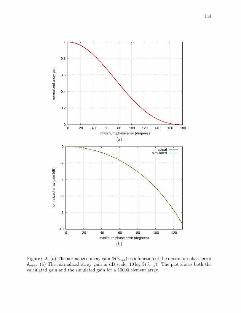
114

0

0.2

0.4

0.6

0.8

1

0 20 40 60 80 100 120 140 160 180

norm

aliz

ed a

rray

gai

n

maximum phase error (degrees)

(a)

-10

-8

-6

-4

-2

0

0 20 40 60 80 100 120

norm

aliz

ed a

rray

gai

n (d

B)

maximum phase error (degrees)

actualsimulated

(b)

Figure 6.2: (a) The normalized array gain Φ(δmax) as a function of the maximum phase errorδmax. (b) The normalized array gain in dB scale, 10 log Φ(δmax). The plot shows both thecalculated gain and the simulated gain for a 10000 element array.

115

-10

-8

-6

-4

-2

0

0 10 20 30 40 50 60 70

norm

aliz

ed a

rray

gai

n (d

B)

standard deviation (degrees)

UniformNormal

Bernoulli

Figure 6.3: Simulated normalized array gain (dB) for a 10000 element array for differentphase error distributions (Uniform, Gaussian, and Bernoulli). For a uniform distribution,the standard deviation is σδ = δmax/

√3.

116

for different array sizes. Figures 6.6ab show that quantization does not increase the widthof the main lobe. Also, notice that when δmax = 180 = π, which corresponds to completelyrandomizing the phase of each antenna, the normalized array response ΦN(π) = 1

N, which

reduces the array gain to that of an omni-directional antenna. So a simple way of creatingan omni-like beam pattern without reducing the radiated power is to choose the phasesrandomly.

6.1.3 Worst case performance analysis

In Sections 6.1.1 and 6.1.2 we analyzed the average (expected) array gain in the presenceof phase errors. In this section, we establish a lower bound on the absolute worst casescenario. Unlike the average case scenario, the worst scenario is a lot more difficult toanalyze especially if the errors are random and cannot be predicted or controlled by thesystem. In this case, the gain can take on any value regardless of how unlikely the eventmight be. For example, if the phase error, or more generally, the weight error can takeon any arbitrary value (e.g. a Gaussian distribution), then the gain be arbitrarily smallwith a nonzero probability. Therefore, to simplify the analysis, we will assume bounded andcontrolled phase errors, which is the case for quantization errors. In the extreme case, wherethe beamforming weights can take only a single value (e.g. 1), the worst case gain can be aslow as zero (occurs when the channel response vector [ejψ1 , . . . , ejψN ]⊤ is orthogonal to the[1, 1, . . . , 1]⊤). We will show that as long as the beamforming weights can take at least twodistinct values, then the array gain in the worst case will still be a constant fraction of themaximum gain independent of the number of antennas.

Let a0 and a1 6= a0 be the two possible complex values for the beamforming weights.We want to show that the ratio of the lower bound minimum gain to the maximum gain isproportional to |a1−a0|2. In order to do that, let us first consider two special cases. In Case1, we can only turn antennas on or off (i.e. the possible beamforming weights are 1 or 0). InCase 2, we assume that the antennas are always on and the possible beamforming weightsare a0 = 1 and a1 = −1.

Let Ψ = ψ1, . . . , ψN be the set of phase responses at the N antennas such that 0 ≤φi < 2π ∀1≤i≤N . If we divide the interval [0, 2π] into 8 equal and contiguous sub-intervals oflength π/4, then we know that one of these intervals will contain at least N/8 of the phaseresponses3. Let Ψmax=π/4 ⊂ Ψ be the subset of phase responses (or antennas) that fall inthat interval. If we choose a beamforming vector w such that wi = 1 if ψi ∈ Ψmax=π/4 andwi = 0 otherwise (Case 1), then the power at the output of the array:

E[|H|2] =

∣∣∣∣∣∣

∑

ψ∈Ψmax=π/4

ejψ

∣∣∣∣∣∣

2

=

∣∣∣∣∣∣

∑

ψ∈Ψmax=π/4

cos(ψ)

∣∣∣∣∣∣

2

+

∣∣∣∣∣∣

∑

ψ∈Ψmax=π/4

sin(ψ)

∣∣∣∣∣∣

2

≥

∣∣∣∣∣∣

∑

ψ∈Ψmax=π/4

cos(ψ)

∣∣∣∣∣∣

2

≥ (N/8)2 cos(π/4)2 = N2/128

3The worst case scenario occurs when the phases are uniformly distributed, in which case each intervalwill contain either ⌊N/8⌋ or ⌈N/8⌉. This is sometimes referred to as the Pigeonhole Principle [49].

117

(a)

-10

-8

-6

-4

-2

0

0 50 100 150 200 250 300 350

quan

tizat

ion

loss

(dB

)

angle (degrees)

10x10 array with wavelength spacing

1-bit2-bit

(b)

-10

-8

-6

-4

-2

0

0 50 100 150 200 250 300 350

quan

tizat

ion

loss

(dB

)

angle (degrees)

10x10 array with half wavelength spacing

1-bit2-bit

(c)

-10

-8

-6

-4

-2

0

0 50 100 150 200 250 300 350

quan

tizat

ion

loss

(dB

)

angle (degrees)

10x10 array with quarter wavelength spacing

1-bit2-bit

Figure 6.4: (a)-(f) Array loss as a result of phase error (quantization) for uniform 10 × 10square array with different inter-element spacings.

118

(a)

-10

-8

-6

-4

-2

0

0 50 100 150 200 250 300 350

quan

tizat

ion

loss

(dB

)

angle (degrees)

100x100 array with wavelength spacing

1-bit2-bit

(b)

-10

-8

-6

-4

-2

0

0 50 100 150 200 250 300 350

quan

tizat

ion

loss

(dB

)

angle (degrees)

100x100 array with half wavelength spacing

1-bit2-bit

(c)

-10

-8

-6

-4

-2

0

0 50 100 150 200 250 300 350

quan

tizat

ion

loss

(dB

)

angle (degrees)

100x100 array with quarter wavelength spacing

1-bit2-bit

Figure 6.5: (a)-(f) Array loss as a result of phase error (quantization) for uniform 100× 100square array with different inter-element spacings.

119

-80

-70

-60

-50

-40

-30

-20

-10

0

0 50 100 150 200 250 300 350

arra

y ga

in (

dB)

angle (degrees)

1-bit2-bit5-bit

(a)

-100

-80

-60

-40

-20

0

50 52 54 56 58 60

arra

y ga

in (

dB)

angle (degrees)

1-bit2-bit3-bit4-bit5-bit

(b)

Figure 6.6: (a)-(b) 2-dimensional horizontal beampattern of a 100x100 array with λ/2 spacing(steered towards 55 degrees) for different phase resolutions.

120

⇒ E[|H|2]/Gmax ≥ 1/128

Therefore, the ratio between the minimum and the maximum gain can be bounded frombelow by a constant that is independent of the number of antennas N . Therefore, thearray gain will continue to grow linearly with N independent of the phase resolution. Theargument can be extended to the second case (1 and -1 complex weights) by making thefollowing observation. When we have two complex signals with phase difference (in absolutevalue) that is π/2 or less, then the magnitude of the sum will be at least as large as themagnitude of the largest of the two. Let cmax=π/4 be the sum of signals in the set Ψmax=π/4

(i.e.∑

ψ∈Ψmax=π/4

ejψ).

Since we can shift the phase of each signal by π (using a1 = −1), we can guarantee thatevery complex signal, before being added, will have a phase difference no larger than π/2with cmax=π/4. Therefore, the minimum gain will grow linearly with N .

Now we can consider the general case where a0 and a1 are arbitrary numbers. Let usdefine the following variables:

∆ = |a0 − a1|, X =∑

ψ∈Ψmax=π/4

ejψ = αN, Y =∑

ψ/∈Ψmax=π/4

ejψ = −βN

Where α and β are complex constants. We showed that |α|2 can be lower bounded by apositive constant that is independent of N . We will also assume without loss of generalitythat a0 = 1, |a1| ≤ 1, and |α| ≥ |β|4. Therefore, the total gain can be expressed in terms ofthese variables5:

G = E[|H|2] = |aiX + ajY |2 = |aiα − ajβ|2N2 =

|α|2|ai − ajβ

α|2N2 = |α|2|ai − ajγ|2N2, where γ = β

α, and 0 ≤ i, j ≤ 1

We want to show that we can choose ai and aj such that we can always guarantee that theterm |α|2|ai−ajγ|2 cannot fall below a constant number gmin = α2∆2/4. This will prove thatthe gain, in the worst case, can be bounded from below by a constant that is independentof the number of antennas N . We have two cases. In the first case, |1 − γ| ≥ ∆/2. In thiscase, choosing ai = aj = a0 = 1 is sufficient to guarantee that the gain does not fall belowthe desired lower bound gmin. In the second case, |1 − γ| < ∆/2. If we choose ai = a0 = 1and aj = a1, then:

α(1 − a1γ) = α(1 − a1 + a1 − a1γ) = α(1 − a1 + a1(1 − γ))

⇒ |α(1 − a1γ)| ≥ |α|(||1 − a1| − |a1||1 − γ||) using the Triangle Inequality

⇒ |α(1 − a1γ)| ≥ |α|(∆ − ∆

2) = |α|∆

2

⇒ |α(1 − a1γ)|2 = |α|2|1 − a1γ)|2 ≥ α2 ∆2

4= gmin

This completes the proof. Notice that gmin → 0 as ∆ → 0 (or a1 → a0), which is what wewould expect.

4We can always reassign the variables to ensure that these conditions hold.5To simplify the proof, we will assume that all complex signals that make up the variable X will be scaled

by the same complex beamforming weight ai, and all complex signals that make up the variable Y will bescaled by the same complex beamforming weight aj . ai and aj need not be equal.

121

6.2 Beam-nulling

In Section 6.1, we analyzed the impact of phase errors on the beamforming gain, andshowed that the gain is very robust in the presence of errors. In this section, we analyze howthe errors impact the interference power, the other component in the SINR6.

In general, adaptive array systems minimize interference by placing beam nulls in thedirections of interfering signals. Controlling the locations of the nulls in the beampatternwill usually require modifying both the phases and amplitudes of the complex beamformingweights, whether the wireless channel is Rayleigh or LOS. In this case, we need to accountfor both phase and amplitude errors. Analyzing the combined effect of phase and amplitudeerrors is easier when we consider the problem in the spatial domain where the optimalcomplex beamforming weights and channel responses can be represented as complex vectorsin the N -dimensional Euclidean space, where N is the number of antennas in the array. Letus assume that we have K +1 complex spatial channel response vectors: a desired vector hd

corresponding to the direction of the desired signal7, and K interferering vectors hi ∀1≤i≤K

corresponding to the directions of K interfering signals.

hd = [α1dejβ1d , . . . , αNde

jβNd ]⊤

hi = [α1iejβ1i , . . . , αNie

jβNi ]⊤ ∀1≤i≤K

The incoming signal at the input of the array y[n] is the sum of the desired signal andinterference and noise:

y[n] = hdd[n] +K∑

i=1

hidi[n] + v[n]

where d[n] is the desired signal, di[n] is interfering signal i, and v[n] is the white noise vectorat the receiver (the variance of each component of v[n] is σ2

v). For simplicity, we shall assumethat the desired and interfering signals have the same power. Using beamforming weightsw (without loss of generality, we can restrict |w| = 1), the signal at the output of the arraywill be wHy[n]. The output SINR is given by:

SINRout =|wHhd|2

|∑Ki=1 wHhi|2 + σ2

v

where (·)H denotes the complex conjugate transpose. Let HI = [h1, . . . ,hK ] be the matrixwhose columns are the interference vectors. Our goal is to achieve maximum interferencerejection while retaining most of the desired signal. This can be achieved by choosing abeamforming weight vector w that is the projection of the desired vector hd onto the subspaceorthogonal to the column space of HI (or the null-space of H⊤

I , which is also known as theleft nullspace of HI), as described in [53]:

wopt = wprojection = hd − HI(HHI HI)

−1HHI hd

6We will assume that the system is interference limited (i.e. the interference power is much larger thanthe noise power).

7In this chapter, we denote scalars in lower case, vectors in bold lower case, and matrices in bold uppercase.

122

The projection-based beamformer is sometimes referred to as the zero-forcing (ZF) beam-former since it completely rejects all the interference (along with any component of thedesired signal that lies in the interference subspace). We can see that rejecting all the in-terfering signals is only possible when the left nullspace is non-empty, which is guaranteedwhen K < N . The projection-based beamformer maximizes the signal to interference ratio(SIR), but not necessarily the SINR since it does not account for noise8. Optimizing theoutput SINR leads to the Minimum Variance Distortionless Response (MVDR) beamformer[33]. If we define the noise+interference correlation matrix RN+I as:

RN+I =K∑

i=1

hihHi + σ2

νIN

where IN is the N ×N identity matrix, then the output SINR can be maximized by choosingwopt:

wopt = wMVDR =R−1

N+Ihd

hHd R−1

N+Ihd

The denominator is a normalizing factor. When the interference power is much larger thanthe noise power, both projection and MVDR yield virtually identical results.

6.2.1 Analysis of Errors in Weights

In this chapter, we focus on interference limited systems (i.e. when interference poweris much larger than the noise floor), in which case both projection and MVDR yield similarresults. Therefore, without loss of generality, we will assume that an optimum beamformerwopt is computed using projection, and wopt takes into account both phase and amplitudeerrors:

wopt = [α1wejβ1w , . . . , αNwejβNw ]⊤

wopt = [α1w(1 + ǫ1)ej(β1w+δ1), . . . , αNw(1 + ǫN)ej(βNw+δN )]⊤

where ǫi ∀1≤i≤N are i.i.d zero mean real random variables with variance E[ǫ2i ] = σ2

ǫ , andδi ∀1≤i≤N are i.i.d zero mean real random variables with variance E[δ2

i ] = σ2δ . We also

assume that the phase and amplitude errors are independent of each other. Furthermore,we scale the weights so that wopt has unit norm (i.e.

∑Ni=1 α2

iw = 1).The phase and amplitude errors result in wopt deviating from wopt by an angle θ. Note

that θ is an angle in N -dimensional space, and does not correspond to a physical direction.This deviation will result in a reduction in the signal strength in the desired direction aswell as an increase in the interference power, since wopt will no longer be orthogonal theinterference subspace. The desired power is proportional to cos(θ), and the increase ininterference (leakage) is proportional to sin(θ) (see Figure 6.7). For small angles θ, we canuse the standard approximations9 sin(θ) ≈ θ and cos(θ) ≈ 1. Thus, we can characterize

8When interference power is near or below the noise floor, complete interference rejection may not result inthe maximum SINR since it might also unnecessarily reduce the power of the desired signal (The componentthat lies in the interference subspace).

9This explains why nulls are more sensitive than peaks to phase and amplitude errors, since sin(θ) changesmore rapidly than cos(θ) when θ is small.

123

the effect of phase and amplitude errors on beam nulls by considering how the mean squareangle σ2

θ(σδ, σǫ, N) = E[θ2] behaves as a function of σδ, σǫ, and N .

Figure 6.7: The optimum beamforming vector wopt can be viewed as a projection of thedesired signal onto the subspace orthogonal to the interference subspace. The distortedbeamforming vector wopt can decomposed into two orthogonal components: wopt = w⊥

opt +

w‖opt. w

‖opt, which is parallel to wopt, represents the potential loss in beamforming gain, and

is proportional to cos(θ). w⊥opt, which is orthogonal to wopt, represents the potential leakage

into the interference subspace, and is proportional to sin(θ).

If we assume that the phase and amplitude variations are small, and given that wopt isunit norm, then we can approximate the error angle θ with the length of the error vector:

∆w = wopt − wopt = [α1wejβ1w(1 − (1 + ǫ1)ejδ1), . . . , αNwejβNw(1 − (1 + ǫN)ejδN )]⊤

We can further simplify the above expression using the approximations cos(δi) ≈ 1, sin(δi) ≈δi, and δiǫi ≈ 0.

∆w = [α1wejβ1w(1 − 1 − ǫ1 − jδ1), . . . , αNwejβNw(1 − 1 − ǫN − jδN)]⊤

= [−α1wejβ1w(ǫ1 + jδ1), . . . ,−αNwejβNw(ǫN + jδN)]⊤

⇒ ‖∆w‖2 = (∆w)H (∆w) =N∑

i=1

α2iw(ǫ2

i + δ2i )

124

By taking the expectation of this expression:

σ2θ ≈ E[‖∆w‖2] = E

[N∑

i=1

α2iw(ǫ2

i + δ2i )

]=

N∑

i=1

α2iw(E[ǫ2

i ] + E[δ2i ])

σ2θ ≈

N∑

i=1

α2iw(σ2

ǫ + σ2δ ) = (σ2

ǫ + σ2δ )

N∑

i=1

α2iw = σ2

ǫ + σ2δ (6.1)

As we can see, the mean square error angle σ2θ is equal to the sum of the mean square

phase error σ2δ and the mean square amplitude error σ2

ǫ . The key conclusion that we drawfrom this result is that the angle error is independent of N , the number of antennas10.

In many phased and adaptive array systems, phase and amplitude control is achieved byindependently modifying the real (in-phase) and imaginary (quadrature) components of thesignal. The results are similar if we consider the error in the real and imaginary parts of thecomponents of the beamforming vector. The proof would proceed in a similar fashion:

wopt = [I1w + jQ1w, . . . , INw + jQNw]⊤, ‖wopt‖2 =N∑

i=1

(I2iw + Q2

iw) = 1

wopt = [I1w(1 + ǫI1) + jQ1w(1 + ǫQ1), . . . , I1w(1 + ǫIN

) + jQ1w(1 + ǫQN)]⊤

where ǫIi∀1≤i≤N are i.i.d zero mean real random variables with variance E[ǫ2

Ii] = σ2

ǫI, and

ǫQi∀1≤i≤N are i.i.d zero mean real random variables with variance E[ǫ2

Qi] = σ2

ǫQ. We assume

that the errors in the real parts and the imaginary parts are independent of each other. Itis also reasonable to assume that σ2

ǫI= σ2

ǫQ, which is very common in practice.

∆w = wopt − wopt =

[I1w(1 − (1 + ǫI1)) + jQ1w(1 − (1 + ǫQ1)), . . . , INw(1 − (1 + ǫIN

)) + jQNw(1 − (1 + ǫQN))]⊤

= [I1wǫI1 + jQ1wǫQ1, . . . , INwǫIN

+ jQNwǫQN]⊤

⇒ ‖∆w‖2 = ∆wH∆w =N∑

i=1

(I2iwǫ2

Ii+ Q2

iwǫ2Qi

)

⇒ σ2θ ≈ E[‖∆w‖2] = E[

N∑

i=1

(I2iwǫ2

Ii+ Q2

iwǫ2Qi

)] =N∑

i=1

(E[I2iw]E[ǫ2

Ii] + E[Q2

iw]E[ǫ2Qi

]) =

N∑

i=1

(E[Iiw]2σ2ǫI

+ E[Q2iw]σ2

ǫQ)

We assume without loss of generality that∑N

i=1 E[I2iw] =

∑Ni=1 E[Q2

iw] = 12

⇒ σ2θ ≈

N∑

i=1

(I2iwσ2

ǫI+ Q2

iwσ2ǫQ

) = σ2ǫI

N∑

i=1

E[I2iw] + σ2

ǫQ

N∑

i=1

E[Q2iw] =

σ2ǫI

+ σ2ǫQ

2(6.2)

The result is very similar to the expression in Equation 6.1.

10The power leakage into the interference subspace is independent of the number of antennas. However,increasing the number of antennas can still increase the output SINR (peak to null ratio) by increasingthe power gain of the desired signal. Increasing the number of antennas also increases the degrees freedomnecessary to null more interferers.

125

6.2.2 Simulation Results

The simulation results shown in Figure 6.8 verify the results in Equations 6.1 and 6.2.The variance of the weights errors E[‖∆w‖2] is shown on the x-axis in Figures 6.8(a)-(d). The variance of the error angle σ2

θ = E[θ2] is shown on the y-axis. We have injectedrandom noise into different components of the complex weight (real, imaginary, phase, andamplitude) separately, represented by the different curves. The different curves show almostexactly the same linear relationship between σ2

θ and the real (in-phase) error (σ2I ), imaginary

(quadrature) error (σ2Q), phase error (σ2

δ ), and amplitude error (σ2ǫ ) as predicted in Equations

6.1 and 6.2. Furthermore, the constant of proportionality is approximately 1 (consistent withthe equations). We repeated the simulations for different values of N (Figures 6.8(b)-(d)),and the results are the same. This shows that the mean square error angle only dependson the magnitude of the errors in the beamforming weight vector and not the number ofantennas, and that the different quantities σ2

δ , σ2ǫ , σ2

I/2 and σ2Q/2 contribute equally to the

overall error angle11.We repeated the same simulations in Figure 6.9 with the interference rejection or leakage

(average interferer power after applying the beamforming weights in the presence of errors)on the y-axis. The results are virtually identical to Figure 6.8. This shows that the averageinterference rejection can be accurately represented by the error angle θ for small values ofθ. This means that the depth of beam nulls is limited by the accuracy of the beamformingweights, and is independent of the size of the array N and the number of interferers K, aslong as N > K12.

For completeness, we also simulated the impact of general errors on the desired signal(beamforming) gain (Figures 6.10, 6.11, and 6.12). These figures show that similar to null-steering, the loss in beamforming depends on the errors in the weight vector, regardless ofwhether the errors are injected directly into the real and imaginary components (Cartesianrepresentation) or phases and amplitudes (polar representation), and is independent of thenumber of antennas N . The figures also show that for a small error angle θ, the normalizedbeamforming gain can be approximated by cos(θ)2.

6.3 Conclusion

In this chapter, we analyzed the array performance loss due to errors in the beamformingweights. We began by considering a beamforming system, which maximizes the gain in adesired direction. We derived an expression for the loss in gain due to uniform phase errors,and provided simulations that validate this result. We showed that beamforming is robustto phase errors. We also derived a lower bound on worst case scenario, and showed thatit is independent of the number of antennas. Then, we considered a beam-nulling system,which rejects interfering signals. We analyzed the effect of uniform amplitude and phaseerrors, and again provided numerical simulations. We showed that the interference rejectionis directly proportional to the magnitude of the errors in the weights, and is independent

11 We have assumed that the different errors (real, imaginary) and (phase, amplitude) and independentof each other and independent across antennas.

12Even though the depth of the null is independent of N , the desired signal power (beamforming gain)grows linearly with N , and thus, the peak to null (signal to interference) ratio grows linearly with N .

126

0

0.02

0.04

0.06

0.08

0.1

0.12

0.14

0.16

0.18

0.2

0 0.02 0.04 0.06 0.08 0.1 0.12 0.14 0.16 0.18 0.2

mea

n sq

uare

err

or a

ngle

σθ2 =

E[θ

2 ]

variance of weight errors

N=50

vs. σδ2

vs. σε2

vs. σδ2+σε

2

vs. σI2/2

vs. σQ2/2

vs. (σI2+σQ

2)/2 0

0.02

0.04

0.06

0.08

0.1

0.12

0.14

0.16

0.18

0.2

0 0.02 0.04 0.06 0.08 0.1 0.12 0.14 0.16 0.18 0.2

mea

n sq

uare

err

or a

ngle

σθ2 =

E[θ

2 ]

variance of weight errors

N=200

vs. σδ2

vs. σε2

vs. σδ2+σε

2

vs. σI2/2

vs. σQ2/2

vs. (σI2+σQ

2)/2

(a) (b)

0

0.02

0.04

0.06

0.08

0.1

0.12

0.14

0.16

0.18

0.2

0 0.02 0.04 0.06 0.08 0.1 0.12 0.14 0.16 0.18 0.2

mea

n sq

uare

err

or a

ngle

σθ2 =

E[θ

2 ]

variance of weight errors

N=400

vs. σδ2

vs. σε2

vs. σδ2+σε

2

vs. σI2/2

vs. σQ2/2

vs. (σI2+σQ

2)/2 0

0.02

0.04

0.06

0.08

0.1

0.12

0.14

0.16

0.18

0.2

0 0.02 0.04 0.06 0.08 0.1 0.12 0.14 0.16 0.18 0.2

mea

n sq

uare

err

or a

ngle

σθ2 =

E[θ

2 ]

variance of weight errors

N=600

vs. σδ2

vs. σε2

vs. σδ2+σε

2

vs. σI2/2

vs. σQ2/2

vs. (σI2+σQ

2)/2

(c) (d)

Figure 6.8: Simulated relationship between weight errors (both phase (σ2δ ), amplitude (σ2

ǫ ),real (σ2

I ), and imaginary (σ2Q)) on the x-axis and the mean square error angle σ2

θ = E[θ2] on

the y-axis: (a) N=50. (b) N=200. (c) N=400. (d) N=600.

127

0

0.02

0.04

0.06

0.08

0.1

0.12

0.14

0.16

0.18

0 0.02 0.04 0.06 0.08 0.1 0.12 0.14 0.16 0.18 0.2

aver

age

inte

rfer

er p

ower

E[|∆

wH

h i|2 ]

variance of weight errors

N=50

vs. σδ2

vs. σε2

vs. σδ2+σε

2

vs. σI2/2

vs. σQ2/2

vs. (σI2+σQ

2)/2 0

0.02

0.04

0.06

0.08

0.1

0.12

0.14

0.16

0.18

0 0.02 0.04 0.06 0.08 0.1 0.12 0.14 0.16 0.18 0.2

aver

age

inte

rfer

er p

ower

E[|∆

wH

h i|2 ]

variance of weight errors

N=200

vs. σδ2

vs. σε2

vs. σδ2+σε

2

vs. σI2/2

vs. σQ2/2

vs. (σI2+σQ

2)/2

(a) (b)

0

0.02

0.04

0.06

0.08

0.1

0.12

0.14

0.16

0.18

0 0.02 0.04 0.06 0.08 0.1 0.12 0.14 0.16 0.18 0.2

aver

age

inte

rfer

er p

ower

E[|∆

wH

h i|2 ]

variance of weight errors

N=400

vs. σδ2

vs. σε2

vs. σδ2+σε

2

vs. σI2/2

vs. σQ2/2

vs. (σI2+σQ

2)/2 0

0.02

0.04

0.06

0.08

0.1

0.12

0.14

0.16

0.18

0 0.02 0.04 0.06 0.08 0.1 0.12 0.14 0.16 0.18 0.2

aver

age

inte

rfer

er p

ower

E[|∆

wH

h i|2 ]

variance of weight errors

N=600

vs. σδ2

vs. σε2

vs. σδ2+σε

2

vs. σI2/2

vs. σQ2/2

vs. (σI2+σQ

2)/2

(c) (d)

Figure 6.9: Simulated relationship between weight errors (both phase (σ2δ ), amplitude (σ2

ǫ ),real (σ2

I ), and imaginary (σ2Q)) on the x-axis and the average interference rejection or leakage

E[|∆Hhi|2] on the y-axis: (a) N=50. (b) 200. (c) N=400. (d) N=600.

128

0.82

0.84

0.86

0.88

0.9

0.92

0.94

0.96

0.98

1

0 0.02 0.04 0.06 0.08 0.1 0.12 0.14 0.16 0.18 0.2

desi

red

sign

al p

ower

(no

rmal

ized

bea

mfo

rmin

g ga

in)

variance of weight errors

N=50

vs. σδ2

vs. σε2

vs. σδ2+σε

2

vs. σI2/2

vs. σQ2/2

vs. (σI2+σQ

2)/2

0.82

0.84

0.86

0.88

0.9

0.92

0.94

0.96

0.98

1

0 0.02 0.04 0.06 0.08 0.1 0.12 0.14 0.16 0.18 0.2

desi

red

sign

al p

ower

(no

rmal

ized

bea

mfo

rmin

g ga

in)

variance of weight errors

N=200

vs. σδ2

vs. σε2

vs. σδ2+σε

2

vs. σI2/2

vs. σQ2/2

vs. (σI2+σQ

2)/2

(a) (b)

0.82

0.84

0.86

0.88

0.9

0.92

0.94

0.96

0.98

1

0 0.02 0.04 0.06 0.08 0.1 0.12 0.14 0.16 0.18 0.2

desi

red

sign

al p

ower

(no

rmal

ized

bea

mfo

rmin

g ga

in)

variance of weight errors

N=400

vs. σδ2

vs. σε2

vs. σδ2+σε

2

vs. σI2/2

vs. σQ2/2

vs. (σI2+σQ

2)/2

0.82

0.84

0.86

0.88

0.9

0.92

0.94

0.96

0.98

1

0 0.02 0.04 0.06 0.08 0.1 0.12 0.14 0.16 0.18 0.2

desi

red

sign

al p

ower

(no

rmal

ized

bea

mfo

rmin

g ga

in)

variance of weight errors

N=600

vs. σδ2

vs. σε2

vs. σδ2+σε

2

vs. σI2/2

vs. σQ2/2

vs. (σI2+σQ

2)/2

(c) (d)

Figure 6.10: Simulated relationship between weight errors (both phase (σ2δ ), amplitude (σ2

ǫ ),real (σ2

I ), and imaginary (σ2Q)) on the x-axis and the average desired signal power (beam-

forming gain) on the y-axis: (a) N=50. (b) 200. (c) N=400. (d) N=600.

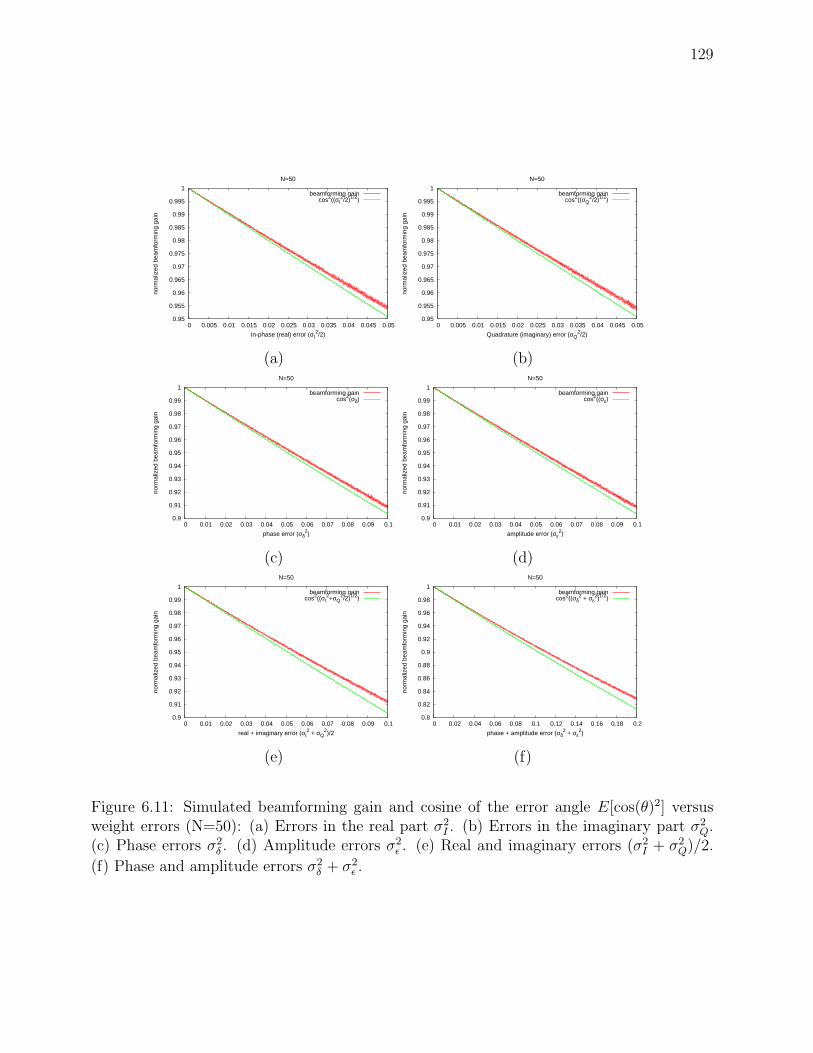
129

0.95

0.955

0.96

0.965

0.97

0.975

0.98

0.985

0.99

0.995

1

0 0.005 0.01 0.015 0.02 0.025 0.03 0.035 0.04 0.045 0.05

norm

aliz

ed b

eam

form

ing

gain

In-phase (real) error (σΙ2/2)

N=50

beamforming gaincos2((σI

2/2)1/2)

0.95

0.955

0.96

0.965

0.97

0.975

0.98

0.985

0.99

0.995

1

0 0.005 0.01 0.015 0.02 0.025 0.03 0.035 0.04 0.045 0.05

norm

aliz

ed b

eam

form

ing

gain

Quadrature (imaginary) error (σQ2/2)

N=50

beamforming gaincos2((σQ

2/2)1/2)

(a) (b)

0.9

0.91

0.92

0.93

0.94

0.95

0.96

0.97

0.98

0.99

1

0 0.01 0.02 0.03 0.04 0.05 0.06 0.07 0.08 0.09 0.1

norm

aliz

ed b

eam

form

ing

gain

phase error (σδ2)

N=50

beamforming gaincos2(σδ)

0.9

0.91

0.92

0.93

0.94

0.95

0.96

0.97

0.98

0.99

1

0 0.01 0.02 0.03 0.04 0.05 0.06 0.07 0.08 0.09 0.1

norm

aliz

ed b

eam

form

ing

gain

amplitude error (σε2)

N=50

beamforming gaincos2((σε)

(c) (d)

0.9

0.91

0.92

0.93

0.94

0.95

0.96

0.97

0.98

0.99

1

0 0.01 0.02 0.03 0.04 0.05 0.06 0.07 0.08 0.09 0.1

norm

aliz

ed b

eam

form

ing

gain

real + imaginary error (σI2 + σQ

2)/2

N=50

beamforming gaincos2((σI

2+σQ2/2)1/2)

0.8

0.82

0.84

0.86

0.88

0.9

0.92

0.94

0.96

0.98

1

0 0.02 0.04 0.06 0.08 0.1 0.12 0.14 0.16 0.18 0.2

norm

aliz

ed b

eam

form

ing

gain

phase + amplitude error (σδ2 + σε

2)

N=50

beamforming gaincos2((σδ

2 + σε2)1/2)

(e) (f)

Figure 6.11: Simulated beamforming gain and cosine of the error angle E[cos(θ)2] versusweight errors (N=50): (a) Errors in the real part σ2

I . (b) Errors in the imaginary part σ2Q.

(c) Phase errors σ2δ . (d) Amplitude errors σ2

ǫ . (e) Real and imaginary errors (σ2I + σ2

Q)/2.

(f) Phase and amplitude errors σ2δ + σ2

ǫ .

130

0.95

0.955

0.96

0.965

0.97

0.975

0.98

0.985

0.99

0.995

1

0 0.005 0.01 0.015 0.02 0.025 0.03 0.035 0.04 0.045 0.05

norm

aliz

ed b

eam

form

ing

gain

In-phase (real) error (σΙ2/2)

N=400

beamforming gaincos2((σI

2/2)1/2)

0.95

0.955

0.96

0.965

0.97

0.975

0.98

0.985

0.99

0.995

1

0 0.005 0.01 0.015 0.02 0.025 0.03 0.035 0.04 0.045 0.05

norm

aliz

ed b

eam

form

ing

gain

Quadrature (imaginary) error (σQ2/2)

N=400

beamforming gaincos2((σQ

2/2)1/2)

(a) (b)

0.9

0.91

0.92

0.93

0.94

0.95

0.96

0.97

0.98

0.99

1

0 0.01 0.02 0.03 0.04 0.05 0.06 0.07 0.08 0.09 0.1

norm

aliz

ed b

eam

form

ing

gain

phase error (σδ2)

N=400

beamforming gaincos2((σδ)

0.9

0.91

0.92

0.93

0.94

0.95

0.96

0.97

0.98

0.99

1

0 0.01 0.02 0.03 0.04 0.05 0.06 0.07 0.08 0.09 0.1

norm

aliz

ed b

eam

form

ing

gain

amplitude error (σε2)

N=400

beamforming gaincos2((σε)

(c) (d)

0.9

0.91

0.92

0.93

0.94

0.95

0.96

0.97

0.98

0.99

1

0 0.01 0.02 0.03 0.04 0.05 0.06 0.07 0.08 0.09 0.1

norm

aliz

ed b

eam

form

ing

gain

real + imaginary error (σI2 + σQ

2)/2

N=400

beamforming gaincos2((σI

2+σQ2/2)1/2)

0.8

0.82

0.84

0.86

0.88

0.9

0.92

0.94

0.96

0.98

1

0 0.02 0.04 0.06 0.08 0.1 0.12 0.14 0.16 0.18 0.2

norm

aliz

ed b

eam

form

ing

gain

phase + amplitude error (σδ2 + σε

2)

N=400

beamforming gaincos2((σδ

2 + σε2)1/2)

(e) (f)

Figure 6.12: Simulated beamforming gain and cosine of the error angle E[cos(θ)2] versusweight errors (N=400): (a) Errors in the real part σ2

I . (b) Errors in the imaginary part σ2Q.

(c) Phase errors σ2δ . (d) Amplitude errors σ2

ǫ . (e) Real and imaginary errors (σ2I + σ2

Q)/2.

(f) Phase and amplitude errors σ2δ + σ2

ǫ .

131

of the number of antennas, assuming that there are more antennas than interferers. A keyconclusion of this chapter is that interference rejection (null-steering) is a lot more sensitiveto errors than beamforming (peak-steering), and in both cases, the performance degradationis independent of the number of antennas.

132

Chapter 7

Error mitigation with vectorquantization

In Chapter 6, we examined how the errors in the beamforming weights affect the signalto noise and interference ratio (SINR) at the output of a beamformer. We showed that thedesired signal component of the SINR is largely insensitive to most phase and amplitudeerrors that occur in practice. However, the interference component is directly proportionalto the magnitude of phase and amplitude errors, and is independent of the number of anten-nas when those errors are uncorrelated. This high sensitivity of beam-nulling (interferencerejection) to errors in the beamforming system can be detrimental for wireless systems thatrely on spatial reuse to increase their capacity. In this chapter, we provide a more in-depthanalysis for one of these sources of error: those that arise from quantizing the beamformingweight vectors. We focus on quantization errors for two reasons. First, whereas most othersources of error (e.g. noise, jitter) are unpredictable, difficult to control and measure, time-varying and independent across antennas, quantization errors can be predicted and shapedby the beamformer. Second, quantization is usually the dominant source of errors in analogbeamforming architectures discussed in Chapter 3 where it is difficult to build high resolutionaccurate beamformers especially at high frequencies1.

The chapter is organized as follows. In Section 7.1, we describe the basic quantizationproblem. In Section 7.2, we present two popular beamforming schemes and analyze theirperformance under the naive scalar quantization approach. We show that in both cases,the signal to interference ratio (SIR) is proportional to the ratio of the antennas to theinterferers (N/K), while the average interferer power is independent of both N and K(consistent with the results derived in Chapter 6). In Section 7.3, we shift the focus tovector quantization techniques. We first derive a lower bound on the achievable SIR undervector quantization, and show that it is quadratic in the number of antennas N (as opposed tolinear in the case of scalar quantization). Next, we present several computationally efficient

The work presented in this chapter was done in collaboration with Mark Johnson, RaghuramanMudumbai, and Upamanyu Madhow [7, 9].

1The LO beamforming architecture presents a bigger challenge because it lacks control over the amplitudeof the signal.

133

vector quantization algorithms, based on greedy coordinate descent (GCD), that achievethis lower bound. We analyze their performance in terms of both achievable SIRs andcomputational complexity. We show that the achievable SIRs are proportional to (N/K)2

(compared to N/K for scalar quantization). These algorithms better exploit the availabledegrees of freedom to cancel interference without much sacrifice in computational efficiencyas we show. Finally, we examine the optimality of GCD based algorithms by comparing themwith the optimum method based on exhaustive search. Our simulation results show that theSIR under optimum quantization can grow exponentially in the number of antennas N . Thisindicates that although the vector quantization techniques proposed in this chapter resultin significant performance gains, they are still far from optimal, and that a computationallytractable algorithm that achieves the upper bound remains an open problem. The resultsin this chapter are based on a combination of mathematical proofs and simulation results.Even though we focus on the Rayleigh channel model because it is easier to analyze, wealso present simulation results based on the line of sight (LOS) channel model (the otherextreme), and show that the results are largely consistent.

7.1 Quantization problem statement

We begin by considering an N -antenna receive beamforming system with the goal ofmaximizing the array gain in the direction of a desired transmitter with respect to theinterfering signals2. For simplicity and without loss of generality, we assume that the desiredtransmitter and the interferers have single antennas. Let hd , [hd[1], hd[2], . . . , hd[N ]]⊤ bethe complex baseband channel response vector from the desired transmitter to the N -antennareceive array3. We similarly denote the channel gain from the lth interferer to the N -antennareceive array as hl , [hl[1], hl[2], . . . , hl[N ]]⊤ for 1 ≤ l ≤ K, where K is the number ofinterferers (K < N). We assume that the components of hd,h1, . . . ,hK are drawn fromzero-mean i.i.d. complex Gaussian distributions, i.e. Rayleigh fading [59]. We assume thatthe variance of the channel gains is unity (i.e. E[|hd[i]|2] = E[|h1[i]|2] = . . . = E[|hK [i]|2] =1 ∀1≤i≤N). This setup can be readily generalized to interferers with different power levelsand to Rician or Line-of-Sight (LOS) channels, and we will present simulation results toshow that the same ideas extend to more general setups4.

Let w = [w[1], . . . , w[N ]]⊤ be the N -element spatial filter (beamforming vector) used bythe receiver to combine the signals from all N antennas. In this case, the SINR at the outputof the receiver (beamformer):

SINR(w) =|wHhd|2∑K

i=1 |wHhi|2 + |wHv|2

2A similar analysis also applies to a transmit array that seeks to minimize its interference at givenlocations. We focus on the receive array for clarity.

3In this chapter, we denote scalars in lower case, vectors in bold lower case, and matrices in bold uppercase.

4Without loss of generality, we assume a narrow band system or a flat fading channel (i.e. a channelresponse that can be represented by a single tap). A frequency-selective (multi-tap) channel can alwaysbe transformed into a group of parallel narrow band subchannels, where each subchannel can be processedindependently (e.g. OFDM).

134

(·)H denotes the conjugate transpose operation, and v is an N -element vector denoting thecomplex white noise signal generated at each antenna element at the receiver (e.g. thermalnoise). We will assume that the system is interference limited (i.e. the interference compo-nent is much larger than the noise). In this case, we can ignore the noise and focus on thesignal to interference ratio (SIR):

SIR(w) =|wHhd|2∑Ki=1 |wHhi|2

Since the beamforming weight vector w appears in both the numerator and the denominator,the SIR does not depend on ‖w‖. Also, let B be the number of available quantization bits(i.e. the I (in-phase or real) and Q (quadrature or imaginary) components of each elementw[i], ∀1≤i≤N of the weight vector w are each quantized to 2B discrete levels). Therefore,there are Nw = 22BN total beamforming weight vectors available from which to choose5.Let W be the set of these discrete weight vectors. We can then formulate the problem ofcomputing the optimal weight as an SIR maximization problem:

wopt , arg maxw∈W

|wHhd|2∑Ki=1 |wHhi|2

Our goal in this chapter, is to compare different strategies for choosing w in terms of both theSIR performance and computational complexity. In order to do so, we need a good metricfor evaluating SIR performance. If one algorithm outperforms another for every possiblerealization of the desire and interference channels, then it is clearly better. However, such adefinition is too stringent to be useful, and in practice, we may have to settle for comparingsome averages. At first glance, it seems as if the natural choice would be to compare theaverage SIR, i.e. E

[SIR

]; however this measure suffers from some fundamental disadvantages.

First of all, it is rather unwieldy analytically. Secondly, the average can be dominated by asmall number of channel realizations where the SIR becomes very large. We therefore choosea different measure: the ratio of average signal power to average interference power:

SIR(w) =E[|wHhd|2]∑Ki=1 E[|wHhi|2]

7.2 Scalar quantization of beamforming weights

In this section, we analyze techniques based on scalar quantization. In scalar quantiza-tion, each component of a beamforming vector is quantized separately to the nearest discretelevel [47]. For simplicity, we assume that the quantization is uniform, and the quantization

5 Note that some of these weight vectors may be scaled versions of others. Therefore, Nw is actuallyan upper-bound on the number of distinct weight vectors available to choose from. Also, since the SIR isindependent of the magnitude of the beamforming weight vector, we can assume without loss of generalitythat the 2B discrete levels are the 2B equal and non-overlapping subintervals between [-1, 1] (i.e. uniformquantization).

135

intervals are obtained by dividing the interval [−1, 1] into 2B equal and contiguous subin-tervals6. The size of the intervals is not relevant to this problem since we can always scalethe beamforming vector without changing the SIR. As a result, scalar quantization can beimplemented by first diving the vector by its real or imaginary components with the largestabsolute value (to ensure that all components lie in the [−1, 1] interval), and then quan-tizing each component (real and imaginary) separately. We shall denote this operation bythe operator QB(·), and thus wq = QB(w) represents the B-bit quantized (and possiblynormalized) version of the vector w. We will also denote the quantization error vector by∆w = w − QB(w). In Chapter 5, we showed that the ability of the beamformer to esti-mate the channel responses does not depend on the accuracy of the beamforming weights.Therefore, we will assume that the beamformer has full knowledge of the channel responseshd,h1,h2, . . . ,hK . We will now consider two strategies for choosing w to improve the SIRand analyze how they are impacted by scalar quantization.

7.2.1 Spatial matched filter

A simple and straight forward choice for the beamforming weight vector is wmf = hd

‖hd‖ ,

also known as the spatial matched filter or maximum ratio combiner (MRC). The spatialmatched filter ensures the maximum attainable signal to noise ratio (SNR). The SIR underthe matched filter is

SIR(wmf) =|wH

mfhd|2∑K

i=1 |wH

mfhi|2

=|hH

d hd|2∑Ki=1 |hH

d hi|2

SIR(wmf) =E[|hH

d hd|2]∑Ki=1 E[|hH

d hi|2]

E[|hHd hd|2] = E[(

N∑

i=1

|hd[i]|2)2] = E[N∑

i=1

N∑

j=1

|hd[i]|2|hd[j]|2]

=N∑

i=1

N∑

j=1

E[|hd[i]|2|hd[j]|2] =N∑

i=1

N∑

j=1,j 6=i

E[|hd[i]|2]E[|hd[j]|2] +N∑

i=1

E[|hd[i]|4]

= N2 − N + 3N = N2 + 2N ∼ N2

E[|hHd hi|2] = E[|

N∑

j=1

h∗d[j]hi[j]|2]

= E[N∑

j=1

N∑

k=1

h∗d[j]hi[j]hd[k]h∗

i [k]]

=N∑

j=1

E[|hd[j]|2]E[|hi[j]|2] = N

6In general, the number and size of each interval will depend on the analog and digital beamformingcircuitry.

136

⇒ SIR(wmf) ∼N

K

Therefore, the average SIR is proportional to NK

. The linear growth with the number ofantennas is due to the beamforming gain which boosts the desired signal power by a factorN , but leaves the interference power almost unchanged because the beamforming weightvector is chosen independent of the channel responses of the interfering signals. Now let’slook at the impact of quantization on the matched filter beamformer. Let wqmf = QB(wmf)

be the matched filter quantized to B bits. The interference should not be affected by thequantization since the beamforming vector is still independent of the channel responses ofthe interfering vectors (i.e. E[|wH

qmfhi|2] = E[|wH

mfhi|2]). In Chapter 6, we showed that the

desired signal (beamforming) gain is robust to errors in the beamfoming weights (the gaindegradation is proportional to the cosine of the error angle). Therefore, even for B = 1, theloss in beamforming is small. Therefore, the quantized matched filter yields similar gain inthe SIR as the matched filter:

SIR(wqmf) ≃ SIR(wmf) ∼N

K(7.1)

In order to support the results derived in this section, we simulated the relationship be-tween the average SIR, as well as its subcomponents (desired signal and interference power),and the number of antennas N , the number of interferers K, and the number of quantiza-tion bits B under the spatial matched filter beamformer. Figure 7.1a shows that the averageSIR, when normalized by the number of antennas N , remains constant as a function of Nfor different quantization levels (B = 1 − 6). Figure 7.1b shows that the average SIR, whenmultiplied by the number of interferers K, remains constant as a function of K. Both theseresults are consistent with Equation 7.1. In Figure 7.2, we simulated the SIR while keepingthe ratio N/K constant. In all the Figures 7.1/7.2, however, we see that using more bitsof resolution slightly improves the SIR by a constant factor independent of both N and K.Figures 7.3/7.4 show that this gain in the SIR is a result of improved beamforming gain andnot interference cancellation (Figures 7.5/7.6). In Figures 7.3/7.4, the SIR is replaced by theaverage desired signal power on y-axis, and the results show a linear growth with N , a slightimprovement with B, and an independence of K. Figures 7.5/7.6 show a constant averageinterferer power independent of N ,K, and B. Therefore, the improvement in average SIRobtained from increasing N and B is due to the desired signal, while the degradation fromincrease in K is due to the interference.

The results in Figures 7.1/7.2, 7.3/7.4, and 7.5/7.6 were obtained using the Rayleighchannel model. We repeated the same simulations under the LOS channel. In Figures7.7/7.8, 7.9/7.10, and 7.11/7.12, we simulated a uniform linear array with λ/2 spacing, andrandomized the azimuth angle of arrival of each transmitter. In Figures 7.137.14, 7.15/7.16,and 7.17/7.18, we simulated a uniform square array with λ/2 spacing, and randomizedthe direction of arrival (in 3 dimensions) of each transmitter. These results show that theperformance of the quantized spatial matched filter is consistent with with Equation 7.1,and is not sensitive to the channel or the quantization resolution.

In addition to being robust to quantization, notice that the matched filter beamformerrequires only computing and quantizing the complex conjugate of the desired channel vector

137

hd and is independent of the interfering channel vectors, and hence it has a low computationalcomplexity O(N).

7.2.2 Zero-Forcing beamformer

In Chapter 6, we showed that complete interference cancellation (nulling) can be achievedby using a beamforming weight vector wzf that is the projection of hd onto the vector sub-space orthogonal to the subspace spanned by the interfering vectors h1, . . . ,hK , a techniquesometimes referred to as zero forcing (ZF) in the signal processing literature. We also showedthat in the presence of errors in the ZF beamformer will result in interference ”leakage” thatis directly proportional to the variance of the errors independent of the number of antennasN . Since quantization is only a special type of errors, the same derivation applies. Sincethe errors will be roughly uniform in the interval [−2−B, 2−B] (within a constant factor), thevariance of the quantization noise σw will be proportional to 2−2B, and the thus the powerof a single interferer will also be proportional to 22B. Therefore, the total interference powerwill be proportional to 2−2BK. Since the desired signal grows linearly with N (beamforminggain), the average SIR at the output of the quantized ZF beamformer wqzf = QB(wzf)

SIR(wqzf) =E[|wH

qzfhd|2]∑K

i=1 E[|wH

qzfhi|2]

∼ N

K22B (7.2)

This result is also supported by the simulation results we present in this section. Unlikethe spatial matched filter, the zero forcing beamformer is a function of both the desired signaland the interfering channel responses. While the SIR at the output of the beamformer growslinearly with the ratio N/K (Figure 7.20(a) shows a constant SIR when N/K is constant),the relationship with both N and K individually is a little more complicated. The reasonis that when hd is projected onto the subspace orthogonal to the interference subspace, welose the component of hd that lies in the interference subspace (h

‖d). When N ≫ K, ‖h‖

d‖will be negligible, and the SIR will be linear in N and 1/K. However, when the interferencesubspace is larger than the orthogonal subspace (K > N/2), there will be significant gainsin increasing N and reducing K. This is shown in Figures 7.19ab, and this is gain inSIR is a result of increasing the desired signal power (Figures 7.21ab). Also, unlike thespatial matched filter, the zero forcing beamformer gets approximately 6dB boost in SIRfor every additional quantization bit (Figures 7.19ab and 7.20ab). This gain in SIR comesmostly from interference rejection component of the SIR, and slightly from the desired signal(Figures 7.23ab, 7.24ab). While the average interferer power at the output of the beamformerdecreases exponentially with the number of quantization bits B, like the spatial matchedfilter, it is largely independent of both N and K. The zero forcing beamformer also differsfrom the spatial matched filter in the dependence of the desired signal on the number ofinterferers. However, the loss in the desired signal power is insignificant compared to thelarge gain obtained from interference nulling.

The results in Figures 7.19/7.20, 7.21/7.22, and 7.23/7.24 were obtained using the Rayleighchannel model. We repeated the same simulations under the LOS channel. In Figures7.25/7.26, 7.9/7.10, and 7.29/7.30, we simulated a uniform linear array with λ/2 spacing,

138

-25

-20

-15

-10

-5

50 100 150 200 250 300 350 400 450 500

10lo

g(E

[SIR

]/N)

number of antennas (N)

Scalar quantizer (matched filter), Rayleigh channel, K=15

B=1B=2B=3B=4B=5B=6

B>30

(a)

15

20

25

30

35

50 100 150 200 250 300 350 400 450

10lo

g(K

*E[S

IR])

number of interferers (K)

Scalar quantizer (matched filter), Rayleigh channel, N=500

B=1B=2B=3B=4B=5B=6

B>30

(b)

Figure 7.1: Simulated (averaged) SIR under the quantized spatial matched filter beamformer(QMF) in a Raleigh channel. (a) SIR (normalized by N in dB scale) as a function of thenumber of antennas N for different quantization levels B (K = 15). (b) SIR (multiplied byK in dB scale) as a function of the number of interferers K for different quantization levelsB (N = 150).

139

-4

-2

0

2

4

6

8

10

20 40 60 80 100 120 140

10lo

g(E

[SIR

])

number of interferers (K)

Scalar quantizer (matched filter), Rayleigh channel, N=3K

B=1B=2B=3B=4B=5B=6

B>30

Figure 7.2: Simulated (averaged) SIR under the quantized spatial matched filter beamformer(QMF) in a Raleigh channel. The SIR (in dB scale) is simulated as a function of the numberof interferers K for different quantization levels B when the ratio N/K = 3.

140

0

0.2

0.4

0.6

0.8

1

50 100 150 200 250 300 350 400 450 500aver

age

norm

aliz

ed d

esire

d si

gnal

pow

er E

[|wqm

fHh d

|2 ]/N

number of antennas (N)

Scalar quantizer (matched filter), Rayleigh channel, K=15

B=1B=2B=3B=4B=5B=6

B>30

(a)

0

0.2

0.4

0.6

0.8

1

50 100 150 200 250 300 350 400 450aver

age

norm

aliz

ed d

esire

d si

gnal

pow

er E

[|wqm

fHh d

|2 ]/N

number of interferers (K)

Scalar quantizer (matched filter), Rayleigh channel, N=500

B=1B=2B=3B=4B=5B=6

B>30

(b)

Figure 7.3: Simulated (averaged) desired signal under the quantized spatial matched filterbeamformer (QMF) in a Raleigh channel. (a) Desired signal (normalized by N) as a functionof the number of antennas N for different quantization levels B (K = 15). (b) Desired signal(normalized by N) as a function of the number of interferers K for different quantizationlevels B (N = 150).

141

0

0.2

0.4

0.6

0.8

1

20 40 60 80 100 120 140aver

age

norm

aliz

ed d

esire

d si

gnal

pow

er E

[|wqm

fHh d

|2 ]/N

number of interferers (K)

Scalar quantizer (matched filter), Rayleigh channel, N=3K

B=1B=2B=3B=4B=5B=6

B>30

Figure 7.4: Simulated (averaged) desired signal under the quantized spatial matched filterbeamformer (QMF) in a Raleigh channel. The desired signal (normalized by N) is simulatedas a function of the number of interferers K for different quantization levels B when the ratioN/K = 3.

142

-10

-5

0

5

10

50 100 150 200 250 300 350 400 450 500

aver

age

inte

rfer

er p

ower

10l

og(E

[|wqm

fHh i

|2 ])

number of antennas (N)

Scalar quantizer (matched filter), Rayleigh channel, K=15

B=1B=2B=3B=4B=5B=6

B>30

(a)

-10

-5

0

5

10

50 100 150 200 250 300 350 400 450

aver

age

inte

rfer

er p

ower

10l

og(E

[|wqm

fHh i

|2 ])

number of interferers (K)

Scalar quantizer (matched filter), Rayleigh channel, N=500

B=1B=2B=3B=4B=5B=6

B>30

(b)

Figure 7.5: Simulated (averaged) power of a single interferer under the quantized spatialmatched filter beamformer (QMF) in a Raleigh channel. (a) Interferer power (in dB scale)as a function of the number of antennas N for different quantization levels B (K = 15).(b) Interferer power (in dB scale) as a function of the number of interferers K for differentquantization levels B (N = 150).

143

-10

-5

0

5

10

20 40 60 80 100 120 140

aver

age

inte

rfer

er p

ower

10l

og(E

[|wqm

fHh i

|2 ])

number of interferers (K)

Scalar quantizer (matched filter), Rayleigh channel, N=3K

B=1B=2B=3B=4B=5B=6

B>30

Figure 7.6: Simulated (averaged) power of a single interferer under the quantized spatialmatched filter beamformer (QMF) in a Raleigh channel. The interferer power (in dB scale)is simulated as a function of the number of interferers K for different quantization levels Bwhen the ratio N/K = 3.

144

-25

-20

-15

-10

-5

0

50 100 150 200 250 300 350 400 450 500

10lo

g(E

[SIR

]/N)

number of antennas (N)

Scalar quantizer (matched filter), LOS (uniform linear array), K=15

B=1B=2B=3B=4B=5B=6

B>30

(a)

15

20

25

30

35

50 100 150 200 250 300 350 400 450

10lo

g(K

*E[S

IR])

number of interferers (K)

Scalar quantizer (matched filter), LOS (uniform linear array), N=500

B=1B=2B=3B=4B=5B=6

B>30

(b)

Figure 7.7: Simulated (averaged) SIR under the quantized spatial matched filter beamformer(QMF) in an LOS channel. In this model, we used a uniform linear array with λ/2 spacing,with all the antennas located on the xy-plane. Both the desired signal and the interferersare located on the xy-plane and their angle of arrival (azimuth) is chosen randomly at eachiteration. (a) SIR (normalized by N in dB scale) as a function of the number of antennasN for different quantization levels B (K = 15). (b) SIR (multiplied by K in dB scale) as afunction of the number of interferers K for different quantization levels B (N = 150).

145

-10

-5

0

5

10

20 40 60 80 100 120 140

10lo

g(E

[SIR

])

number of interferers (K)

Scalar quantizer (matched filter), LOS (uniform linear array), N=3K

B=1B=2B=3B=4B=5B=6

B>30

Figure 7.8: Simulated (averaged) SIR under the quantized spatial matched filter beamformer(QMF) in an LOS channel. In this model, we used a uniform linear array with λ/2 spacing,with all the antennas located on the xy-plane. Both the desired signal and the interferersare located on the xy-plane and their angle of arrival (azimuth) is chosen randomly at eachiteration. The SIR (in dB scale) is simulated as a function of the number of interferers Kfor different quantization levels B when the ratio N/K = 3.

146

0

0.2

0.4

0.6

0.8

1

50 100 150 200 250 300 350 400 450 500aver

age

norm

aliz

ed d

esire

d si

gnal

pow

er E

[|wqm

fHh d

|2 ]/N

number of antennas (N)

Scalar quantizer (matched filter), LOS (uniform linear array), K=15

B=1B=2B=3B=4B=5B=6

B>30

(a)

0

0.2

0.4

0.6

0.8

1

50 100 150 200 250 300 350 400 450aver

age

norm

aliz

ed d

esire

d si

gnal

pow

er E

[|wqm

fHh d

|2 ]/N

number of interferers (K)

Scalar quantizer (matched filter), LOS (uniform linear array), N=500

B=1B=2B=3B=4B=5B=6

B>30

(b)

Figure 7.9: Simulated (averaged) desired signal under the quantized spatial matched filterbeamformer (QMF) in an LOS channel. In this model, we used a uniform linear arraywith λ/2 spacing, with all the antennas located on the xy-plane. Both the desired signaland the interferers are located on the xy-plane and their angle of arrival (azimuth) is chosenrandomly at each iteration. (a) Desired signal (normalized by N) as a function of the numberof antennas N for different quantization levels B (K = 15). (b) Desired signal (normalized byN) as a function of the number of interferers K for different quantization levels B (N = 150).

147

0

0.2

0.4

0.6

0.8

1

20 40 60 80 100 120 140aver

age

norm

aliz

ed d

esire

d si

gnal

pow

er E

[|wqm

fHh d

|2 ]/N

number of interferers (K)

Scalar quantizer (matched filter), LOS (uniform linear array), N=3K

B=1B=2B=3B=4B=5B=6

B>30

Figure 7.10: Simulated (averaged) desired signal under the quantized spatial matched filterbeamformer (QMF) in an LOS channel. In this model, we used a uniform linear array withλ/2 spacing, with all the antennas located on the xy-plane. Both the desired signal andthe interferers are located on the xy-plane and their angle of arrival (azimuth) is chosenrandomly at each iteration. The desired signal (normalized by N) is simulated as a functionof the number of interferers K for different quantization levels B when the ratio N/K = 3.

148

-10

-5

0

5

10

15

50 100 150 200 250 300 350 400 450 500

aver

age

inte

rfer

er p

ower

10l

og(E

[|wqm

fHh i

|2 ])

number of antennas (N)

Scalar quantizer (matched filter), LOS (uniform linear array), K=15

B=1B=2B=3B=4B=5B=6

B>30

(a)

-10

-5

0

5

10

15

50 100 150 200 250 300 350 400 450

aver

age

inte

rfer

er p

ower

10l

og(E

[|wqm

fHh i

|2 ])

number of interferers (K)

Scalar quantizer (matched filter), LOS (uniform linear array), N=500

B=1B=2B=3B=4B=5B=6

B>30

(b)

Figure 7.11: Simulated (averaged) power of a single interferer under the quantized spatialmatched filter beamformer (QMF) in an LOS channel. In this model, we used a uniformlinear array with λ/2 spacing, with all the antennas located on the xy-plane. Both the desiredsignal and the interferers are located on the xy-plane and their angle of arrival (azimuth) ischosen randomly at each iteration. (a) Interferer power (in dB scale) as a function of thenumber of antennas N for different quantization levels B (K = 15). (b) Interferer power(in dB scale) as a function of the number of interferers K for different quantization levels B(N = 150).

149

-10

-5

0

5

10

15

20 40 60 80 100 120 140

aver

age

inte

rfer

er p

ower

10l

og(E

[|wqm

fHh i

|2 ])

number of interferers (K)

Scalar quantizer (matched filter), LOS (uniform linear array), N=3K

B=1B=2B=3B=4B=5B=6

B>30

Figure 7.12: Simulated (averaged) power of a single interferer under the quantized spatialmatched filter beamformer (QMF) in an LOS channel. In this model, we used a uniformlinear array with λ/2 spacing, with all the antennas located on the xy-plane. Both the desiredsignal and the interferers are located on the xy-plane and their angle of arrival (azimuth)is chosen randomly at each iteration. The interferer power (in dB scale) is simulated as afunction of the number of interferers K for different quantization levels B when the ratioN/K = 3.

150

-25

-20

-15

-10

-5

0

100 200 300 400 500

10lo

g(E

[SIR

]/N)

number of antennas (N)

Scalar quantizer (matched filter), LOS (uniform square array), K=15

B=1B=2B=3B=4B=5B=6

B>30

(a)

15

20

25

30

35

40

50 100 150 200 250 300 350 400 450

10lo

g(K

*E[S

IR])

number of interferers (K)

Scalar quantizer (matched filter), LOS (uniform square array), N=625

B=1B=2B=3B=4B=5B=6

B>30

(b)

Figure 7.13: Simulated (averaged) SIR under the quantized spatial matched filter beam-former (QMF) in an LOS channel. In this model, we used a uniform square array with λ/2spacing. Both the desired signal and the interferers are placed randomly on the surface of alarge sphere (in the far field of the array) centered around the origin at each iteration. (a)SIR (normalized by N in dB scale) as a function of the number of antennas N for differentquantization levels B (K = 15). (b) SIR (multiplied by K in dB scale) as a function of thenumber of interferers K for different quantization levels B (N = 150).

151

-10

-5

0

5

10

20 40 60 80 100 120 140

10lo

g(E

[SIR

])

number of interferers (K)

Scalar quantizer (matched filter), LOS (uniform square array), N=3K

B=1B=2B=3B=4B=5B=6

B>30

Figure 7.14: Simulated (averaged) SIR under the quantized spatial matched filter beam-former (QMF) in an LOS channel. In this model, we used a uniform square array with λ/2spacing. Both the desired signal and the interferers are placed randomly on the surface ofa large sphere (in the far field of the array) centered around the origin at each iteration.The SIR (in dB scale) is simulated as a function of the number of interferers K for differentquantization levels B when the ratio N/K = 3.

152

0

0.2

0.4

0.6

0.8

1

100 200 300 400 500 600aver

age

norm

aliz

ed d

esire

d si

gnal

pow

er E

[|wqm

fHh d

|2 ]/N

number of antennas (N)

Scalar quantizer (matched filter), LOS (uniform square array), K=15

B=1B=2B=3B=4B=5B=6

B>30

(a)

0

0.2

0.4

0.6

0.8

1

50 100 150 200 250 300 350 400 450aver

age

norm

aliz

ed d

esire

d si

gnal

pow

er E

[|wqm

fHh d

|2 ]/N

number of interferers (K)

Scalar quantizer (matched filter), LOS (uniform square array), N=625

B=1B=2B=3B=4B=5B=6

B>30

(b)

Figure 7.15: Simulated (averaged) desired signal under the quantized spatial matched filterbeamformer (QMF) in an LOS channel. In this model, we used a uniform square array withλ/2 spacing. Both the desired signal and the interferers are placed randomly on the surfaceof a large sphere (in the far field of the array) centered around the origin at each iteration.(a) Desired signal (normalized by N) as a function of the number of antennas N for differentquantization levels B (K = 15). (b) Desired signal (normalized by N) as a function of thenumber of interferers K for different quantization levels B (N = 150).

153

0

0.2

0.4

0.6

0.8

1

20 40 60 80 100 120 140aver

age

norm

aliz

ed d

esire

d si

gnal

pow

er E

[|wqm

fHh d

|2 ]/N

number of interferers (K)

Scalar quantizer (matched filter), LOS (uniform square array), N=3K

B=1B=2B=3B=4B=5B=6

B>30

Figure 7.16: Simulated (averaged) desired signal under the quantized spatial matched filterbeamformer (QMF) in an LOS channel. In this model, we used a uniform square array withλ/2 spacing. Both the desired signal and the interferers are placed randomly on the surfaceof a large sphere (in the far field of the array) centered around the origin at each iteration.The desired signal (normalized by N) is simulated as a function of the number of interferersK for different quantization levels B when the ratio N/K = 3.

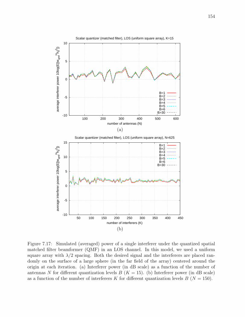
154

-10

-5

0

5

10

100 200 300 400 500 600

aver

age

inte

rfer

er p

ower

10l

og(E

[|wqm

fHh i

|2 ])

number of antennas (N)

Scalar quantizer (matched filter), LOS (uniform square array), K=15

B=1B=2B=3B=4B=5B=6

B>30

(a)

-10

-5

0

5

10

15

50 100 150 200 250 300 350 400 450

aver

age

inte

rfer

er p

ower

10l

og(E

[|wqm

fHh i

|2 ])

number of interferers (K)

Scalar quantizer (matched filter), LOS (uniform square array), N=625

B=1B=2B=3B=4B=5B=6

B>30

(b)

Figure 7.17: Simulated (averaged) power of a single interferer under the quantized spatialmatched filter beamformer (QMF) in an LOS channel. In this model, we used a uniformsquare array with λ/2 spacing. Both the desired signal and the interferers are placed ran-domly on the surface of a large sphere (in the far field of the array) centered around theorigin at each iteration. (a) Interferer power (in dB scale) as a function of the number ofantennas N for different quantization levels B (K = 15). (b) Interferer power (in dB scale)as a function of the number of interferers K for different quantization levels B (N = 150).

155

-10

-5

0

5

10

15

20 40 60 80 100 120 140

aver

age

inte

rfer

er p

ower

10l

og(E

[|wqm

fHh i

|2 ])

number of interferers (K)

Scalar quantizer (matched filter), LOS (uniform square array), N=3K

B=1B=2B=3B=4B=5B=6

B>30

Figure 7.18: Simulated (averaged) power of a single interferer under the quantized spatialmatched filter beamformer (QMF) in an LOS channel. In this model, we used a uniformsquare array with λ/2 spacing. Both the desired signal and the interferers are placed ran-domly on the surface of a large sphere (in the far field of the array) centered around theorigin at each iteration. The interferer power (in dB scale) is simulated as a function of thenumber of interferers K for different quantization levels B when the ratio N/K = 3.

156

and randomized the azimuth angle of arrival of each transmitter. In Figures 7.31/7.32,7.33/7.34, and 7.35/7.36, we simulated a uniform square array with λ/2 spacing, and ran-domized the direction of arrival (in 3 dimensions) of each transmitter. These results showthat the performance of the quantized spatial matched filter is consistent with with Equation7.2 independent of the channel model.

The quantized ZF beamformer improves the average SIR/interference rejection by a factorof 22B relative to the spatial matched filter. However, this improved SIR comes at theexpense of increased computational complexity. Since the quantized ZF beamformer requiressolving an N × K complex least squares problem, the overall computational complexity isO(NK2). In both cases, however, the interference leakage remains independent of the numberof antennas N .

7.3 Vector quantization of antenna weights

In Section 7.2, we showed that a naive strategy of coefficient-by-coefficient quantizationof the beamforming weights is not very efficient: the average SIR scales as N/K. That is,we obtain the combining gains for the desired signal, but increasing the number of degreesof freedom N does not lead to any improved scaling in the residual interference powerat the output of the beamformer. In this section, we explore more sophisticated vectorquantization strategies. In Section 7.3.1, we establish an analytical lower bound on theexpected SIR improvement using vector quantization techniques. In Section 7.3.2, we proposethree computationally efficient vector quantization schemes and analyze their performance,optimality, and complexity as a function of N , K, and B. Finally, in Section 7.3.3, weanalyze the beamforming gain using vector quantization techniques.

7.3.1 An approximate lower bound on achievable SIR

In [7], we showed that the SIR that can be achieved by intelligently choosing the quantizedweights has a lower bound that grows quadratically with the number of antennas N . Theproof idea is very simple and intuitive. We can think of the problem of choosing the optimalweight vector w as a problem of choosing the optimal error vector ∆w. Our goal is to showthat when the components of ∆w are chosen dependently of each other, the interferencepower can be made to decrease significantly with N (as opposed being independent of Nwhen the components are chosen independently).

For simplicity, we will assume a single interferer or K = 1 (The extension to the moregeneral case K > 1 is straight forward). Our goal is to minimize the term |∆wHh1|2,when the coefficients of h1 are independent zero-mean complex Gaussian random variableswith unit variance (i.e. Rayleigh channel coefficients). Let’s start by considering a simplerproblem. Suppose we simply wish to minimize |uHh1|2, where u takes all possible values inU = 1√

N−1, +1N (i.e. the elements of U are binary vectors normalized to unit norm). Let

T (u) , uHh1. Note that T (u) ∼ CN(0, 1) for any u ∈ U since the coefficients of h1 arealso assumed to be CN(0, 1). Therefore, T (u1), T (u2) are jointly complex Gaussian withcovariance equal to uH

1 u2. We now take a subset Uo ⊂ U which forms an orthonormal basisin N dimensions: the Walsh-Hadamard codes [29]. Then T (u) : u ∈ Uo are N independent

157

-15

-10

-5

0

5

10

15

20

50 100 150 200 250 300 350 400 450 500

10lo

g(E

[SIR

]/N)

number of antennas (N)

Scalar quantizer (zero forcing), Rayleigh channel, K=15

B=2B=3B=4B=5B=6

(a)

20

25

30

35

40

45

50

55

60

65

50 100 150 200 250 300 350 400 450

10lo

g(K

*E[S

IR])

number of interferers (K)

Scalar quantizer (zero forcing), Rayleigh channel, N=500

B=2B=3B=4B=5B=6

(b)

Figure 7.19: Simulated (averaged) SIR under the quantized zero-forcing beamformer (QZF)in a Raleigh channel. (a) SIR (normalized by N in dB scale) as a function of the numberof antennas N for different quantization levels B (K = 15). (b) SIR (multiplied by K indB scale) as a function of the number of interferers K for different quantization levels B(N = 150).

158

5

10

15

20

25

30

35

40

45

50

20 40 60 80 100 120 140

10lo

g(E

[SIR

])

number of interferers (K)

Scalar quantizer (zero forcing), Rayleigh channel, N=3K

B=2B=3B=4B=5B=6

(a)

0

5

10

15

20

25

30

35

2 2.5 3 3.5 4 4.5 5 5.5 6

10lo

g(E

[SIR

])

number of bits (B)

Scalar quantizer (zero forcing), Rayleigh channel, N=500, K=250

QZF6dB/bit

(b)

Figure 7.20: Simulated (averaged) SIR under the quantized zero-forcing beamformer (QZF)in a Raleigh channel. (a) SIR (in dB scale) as a function of the number of interferers K fordifferent quantization levels B when the ratio N/K = 3. (b) SIR (in dB scale) as a functionof the quantization level B for N=500 and K=250.

159

0

0.2

0.4

0.6

0.8

1

50 100 150 200 250 300 350 400 450 500aver

age

norm

aliz

ed d

esire

d si

gnal

pow

er E

[|wqz

fHh d

|2 ]/N

number of antennas (N)

Scalar quantizer (zero forcing), Rayleigh channel, K=15

B=2B=3B=4B=5B=6

(a)

0

0.2

0.4

0.6

0.8

1

50 100 150 200 250 300 350 400 450aver

age

norm

aliz

ed d

esire

d si

gnal

pow

er E

[|wqz

fHh d

|2 ]/N

number of interferers (K)

Scalar quantizer (zero forcing), Rayleigh channel, N=500

B=2B=3B=4B=5B=6

(b)

Figure 7.21: Simulated (averaged) desired signal under the quantized zero-forcing beam-former (QZF) in a Raleigh channel. (a) Desired signal (normalized by N) as a function ofthe number of antennas N for different quantization levels B (K = 15). (b) Desired signal(normalized by N) as a function of the number of interferers K for different quantizationlevels B (N = 150).

160

0

0.2

0.4

0.6

0.8

1

20 40 60 80 100 120 140aver

age

norm

aliz

ed d

esire

d si

gnal

pow

er E

[|wqz

fHh d

|2 ]/N

number of interferers (K)

Scalar quantizer (zero forcing), Rayleigh channel, N=3K

B=2B=3B=4B=5B=6

Figure 7.22: Simulated (averaged) desired signal under the quantized zero-forcing beam-former (QZF) in a Raleigh channel. The desired signal (normalized by N) is simulated asa function of the number of interferers K for different quantization levels B when the ratioN/K = 3.

161

-45

-40

-35

-30

-25

-20

-15

-10

-5

0

50 100 150 200 250 300 350 400 450 500

aver

age

inte

rfer

er p

ower

10l

og(E

[|wqz

fHh i

|2 ])

number of antennas (N)

Scalar quantizer (zero forcing), Rayleigh channel, K=15

B=2B=3B=4B=5B=6

(a)

-30

-25

-20

-15

-10

-5

0

5

50 100 150 200 250 300 350 400 450

aver

age

inte

rfer

er p

ower

10l

og(E

[|wqz

fHh i

|2 ])

number of interferers (K)

Scalar quantizer (zero forcing), Rayleigh channel, N=500

B=2B=3B=4B=5B=6

(b)

Figure 7.23: Simulated (averaged) power of a single interferer under the quantized zero-forcing beamformer (QZF) in a Raleigh channel. (a) Interferer power (in dB scale) as afunction of the number of antennas N for different quantization levels B (K = 15). (b)Interferer power (in dB scale) as a function of the number of interferers K for differentquantization levels B (N = 150).

162

-35

-30

-25

-20

-15

-10

-5

0

5

60 80 100 120 140

aver

age

inte

rfer

er p

ower

10l

og(E

[|wqz

fHh i

|2 ])

number of interferers (K)

Scalar quantizer (zero forcing), Rayleigh channel, N=3K

B=2B=3B=4B=5B=6

(a)

-35

-30

-25

-20

-15

-10

-5

2 2.5 3 3.5 4 4.5 5 5.5 6

aver

age

inte

rfer

er p

ower

10l

og(E

[|wqz

fHh i

|2 ])

number of bits (B)

Scalar quantizer (zero forcing), Rayleigh channel, N=500, K=250

QZF6dB/bit

(b)

Figure 7.24: Simulated (averaged) power of a single interferer under the quantized zero-forcing beamformer (QZF) in a Raleigh channel. (a) Interferer power (in dB scale) as afunction of the number of interferers K for different quantization levels B when the ratioN/K = 3. (b) Interferer power (in dB scale) as a function of the quantization level B forN=500 and K=250.

163

-15

-10

-5

0

5

10

15

20

25

30

50 100 150 200 250 300 350 400 450 500

10lo

g(E

[SIR

]/N)

number of antennas (N)

Scalar quantizer (zero forcing), LOS (uniform linear array), K=15

B=2B=3B=4B=5B=6

(a)

15

20

25

30

35

40

45

50

55

60

65

50 100 150 200 250 300 350 400 450

10lo

g(K

*E[S

IR])

number of interferers (K)

Scalar quantizer (zero forcing), LOS (uniform linear array), N=500

B=2B=3B=4B=5B=6

(b)

Figure 7.25: Simulated (averaged) SIR under the quantized zero-forcing beamformer (QZF)in an LOS channel. In this model, we used a uniform linear array with λ/2 spacing, with allthe antennas located on the xy-plane. Both the desired signal and the interferers are locatedon the xy-plane and their angle of arrival (azimuth) is chosen randomly at each iteration. (a)SIR (normalized by N in dB scale) as a function of the number of antennas N for differentquantization levels B (K = 15). (b) SIR (multiplied by K in dB scale) as a function of thenumber of interferers K for different quantization levels B (N = 150).

164

5

10

15

20

25

30

35

40

45

50

20 40 60 80 100 120 140

10lo

g(E

[SIR

])

number of interferers (K)

Scalar quantizer (zero forcing), LOS (uniform linear array), N=3K

B=2B=3B=4B=5B=6

(a)

0

5

10

15

20

25

30

2 2.5 3 3.5 4 4.5 5 5.5 6

10lo

g(E

[SIR

])

number of bits (B)

Scalar quantizer (zero forcing), LOS (uniform linear array), N=500, K=250

QZF6dB/bit

(b)

Figure 7.26: Simulated (averaged) SIR under the quantized zero-forcing beamformer (QZF)in an LOS channel. In this model, we used a uniform linear array with λ/2 spacing, with allthe antennas located on the xy-plane. Both the desired signal and the interferers are locatedon the xy-plane and their angle of arrival (azimuth) is chosen randomly at each iteration.(a) SIR (in dB scale) as a function of the number of interferers K for different quantizationlevels B when the ratio N/K = 3. (b) SIR (in dB scale) as a function of the quantizationlevel B for N=500 and K=250.

165

0

0.2

0.4

0.6

0.8

1

50 100 150 200 250 300 350 400 450 500aver

age

norm

aliz

ed d

esire

d si

gnal

pow

er E

[|wqz

fHh d

|2 ]/N

number of antennas (N)

Scalar quantizer (zero forcing), LOS (uniform linear array), K=15

B=2B=3B=4B=5B=6

(a)

0

0.2

0.4

0.6

0.8

1

50 100 150 200 250 300 350 400 450aver

age

norm

aliz

ed d

esire

d si

gnal

pow

er E

[|wqz

fHh d

|2 ]/N

number of interferers (K)

Scalar quantizer (zero forcing), LOS (uniform linear array), N=500

B=2B=3B=4B=5B=6

(b)

Figure 7.27: Simulated (averaged) desired signal under the quantized zero-forcing beam-former (QZF) in an LOS channel. In this model, we used a uniform linear array with λ/2spacing, with all the antennas located on the xy-plane. Both the desired signal and the inter-ferers are located on the xy-plane and their angle of arrival (azimuth) is chosen randomly ateach iteration. (a) Desired signal (normalized by N) as a function of the number of antennasN for different quantization levels B (K = 15). (b) Desired signal (normalized by N) as afunction of the number of interferers K for different quantization levels B (N = 150).

166

0

0.2

0.4

0.6

0.8

1

20 40 60 80 100 120 140aver

age

norm

aliz

ed d

esire

d si

gnal

pow

er E

[|wqz

fHh d

|2 ]/N

number of interferers (K)

Scalar quantizer (zero forcing), LOS (uniform linear array), N=3K

B=2B=3B=4B=5B=6

Figure 7.28: Simulated (averaged) desired signal under the quantized zero-forcing beam-former (QZF) in an LOS channel. In this model, we used a uniform linear array with λ/2spacing, with all the antennas located on the xy-plane. Both the desired signal and the in-terferers are located on the xy-plane and their angle of arrival (azimuth) is chosen randomlyat each iteration. The desired signal (normalized by N) is simulated as a function of thenumber of interferers K for different quantization levels B when the ratio N/K = 3.

167

-40

-35

-30

-25

-20

-15

-10

-5

0

5

50 100 150 200 250 300 350 400 450 500

aver

age

inte

rfer

er p

ower

10l

og(E

[|wqz

fHh i

|2 ])

number of antennas (N)

Scalar quantizer (zero forcing), LOS (uniform linear array), K=15

B=2B=3B=4B=5B=6

(a)

-40

-35

-30

-25

-20

-15

-10

-5

0

5

20 40 60 80 100 120 140

aver

age

inte

rfer

er p

ower

10l

og(E

[|wqz

fHh i

|2 ])

number of interferers (K)

Scalar quantizer (zero forcing), LOS (uniform linear array), N=500

B=2B=3B=4B=5B=6

(b)

Figure 7.29: Simulated (averaged) power of a single interferer under the quantized zero-forcing beamformer (QZF) in an LOS channel. In this model, we used a uniform linear arraywith λ/2 spacing, with all the antennas located on the xy-plane. Both the desired signaland the interferers are located on the xy-plane and their angle of arrival (azimuth) is chosenrandomly at each iteration. (a) Interferer power (in dB scale) as a function of the number ofantennas N for different quantization levels B (K = 15). (b) Interferer power (in dB scale)as a function of the number of interferers K for different quantization levels B (N = 150).

168

-35

-30

-25

-20

-15

-10

-5

0

5

20 40 60 80 100 120 140

aver

age

inte

rfer

er p

ower

10l

og(E

[|wqz

fHh i

|2 ])

number of interferers (K)

Scalar quantizer (zero forcing), LOS (uniform linear array), N=3K

B=2B=3B=4B=5B=6

(a)

-35

-30

-25

-20

-15

-10

-5

2 2.5 3 3.5 4 4.5 5 5.5 6

aver

age

inte

rfer

er p

ower

10l

og(E

[|wqz

fHh i

|2 ])

number of bits (B)

Scalar quantizer (zero forcing), LOS (uniform linear array), N=500, K=250

QZF6dB/bit

(b)

Figure 7.30: Simulated (averaged) power of a single interferer under the quantized zero-forcing beamformer (QZF) in an LOS channel. In this model, we used a uniform linear arraywith λ/2 spacing, with all the antennas located on the xy-plane. Both the desired signaland the interferers are located on the xy-plane and their angle of arrival (azimuth) is chosenrandomly at each iteration. (a) Interferer power (in dB scale) as a function of the numberof interferers K for different quantization levels B when the ratio N/K = 3. (b) Interfererpower (in dB scale) as a function of the quantization level B for N=500 and K=250.

169

-20

-15

-10

-5

0

5

10

15

20

25

100 200 300 400 500 600

10lo

g(E

[SIR

]/N)

number of antennas (N)

Scalar quantizer (zero forcing), LOS (uniform square array), K=15

B=2B=3B=4B=5B=6

(a)

20

25

30

35

40

45

50

55

60

65

50 100 150 200 250 300 350 400 450

10lo

g(K

*E[S

IR])

number of interferers (K)

Scalar quantizer (zero forcing), LOS (uniform square array), N=625

B=2B=3B=4B=5B=6

(b)

Figure 7.31: Simulated (averaged) SIR under the quantized zero-forcing beamformer (QZF)in an LOS channel. In this model, we used a uniform square array with λ/2 spacing. Boththe desired signal and the interferers are placed randomly on the surface of a large sphere (inthe far field of the array) centered around the origin at each iteration. (a) SIR (normalizedby N in dB scale) as a function of the number of antennas N for different quantization levelsB (K = 15). (b) SIR (multiplied by K in dB scale) as a function of the number of interferersK for different quantization levels B (N = 150).

170

5

10

15

20

25

30

35

40

45

50

20 40 60 80 100 120 140

10lo

g(E

[SIR

])

number of interferers (K)

Scalar quantizer (zero forcing), LOS (uniform square array), N=3K

B=2B=3B=4B=5B=6

(a)

0

5

10

15

20

25

30

2 2.5 3 3.5 4 4.5 5 5.5 6

10lo

g(E

[SIR

])

number of bits (B)

Scalar quantizer (zero forcing), LOS (uniform square array), N=625, K=310

QZF6dB/bit

(b)

Figure 7.32: Simulated (averaged) SIR under the quantized zero-forcing beamformer (QZF)in an LOS channel. In this model, we used a uniform square array with λ/2 spacing. Boththe desired signal and the interferers are placed randomly on the surface of a large sphere (inthe far field of the array) centered around the origin at each iteration. (a) SIR (in dB scale)as a function of the number of interferers K for different quantization levels B when theratio N/K = 3. (b) SIR (in dB scale) as a function of the quantization level B for N=500and K=250.

171

0

0.2

0.4

0.6

0.8

1

100 200 300 400 500 600aver

age

norm

aliz

ed d

esire

d si

gnal

pow

er E

[|wqz

fHh d

|2 ]/N

number of antennas (N)

Scalar quantizer (zero forcing), LOS (uniform square array), K=15

B=2B=3B=4B=5B=6

(a)

0

0.2

0.4

0.6

0.8

1

50 100 150 200 250 300 350 400 450aver

age

norm

aliz

ed d

esire

d si

gnal

pow

er E

[|wqz

fHh d

|2 ]/N

number of interferers (K)

Scalar quantizer (zero forcing), LOS (uniform square array), N=625

B=2B=3B=4B=5B=6

(b)

Figure 7.33: Simulated (averaged) desired signal under the quantized zero-forcing beam-former (QZF) in an LOS channel. In this model, we used a uniform square array with λ/2spacing. Both the desired signal and the interferers are placed randomly on the surface of alarge sphere (in the far field of the array) centered around the origin at each iteration. (a)Desired signal (normalized by N) as a function of the number of antennas N for differentquantization levels B (K = 15). (b) Desired signal (normalized by N) as a function of thenumber of interferers K for different quantization levels B (N = 150).

172

0

0.2

0.4

0.6

0.8

1

20 40 60 80 100 120 140aver

age

norm

aliz

ed d

esire

d si

gnal

pow

er E

[|wqz

fHh d

|2 ]/N

number of interferers (K)

Scalar quantizer (zero forcing), LOS (uniform square array), N=3K

B=2B=3B=4B=5B=6

Figure 7.34: Simulated (averaged) desired signal under the quantized zero-forcing beam-former (QZF) in an LOS channel. In this model, we used a uniform square array with λ/2spacing. Both the desired signal and the interferers are placed randomly on the surface of alarge sphere (in the far field of the array) centered around the origin at each iteration. Thedesired signal (normalized by N) is simulated as a function of the number of interferers Kfor different quantization levels B when the ratio N/K = 3.

173

-40

-35

-30

-25

-20

-15

-10

-5

100 200 300 400 500 600

aver

age

inte

rfer

er p

ower

10l

og(E

[|wqz

fHh i

|2 ])

number of antennas (N)

Scalar quantizer (zero forcing), LOS (uniform square array), K=15

B=2B=3B=4B=5B=6

(a)

-40

-35

-30

-25

-20

-15

-10

-5

0

5

50 100 150 200 250 300 350 400 450

aver

age

inte

rfer

er p

ower

10l

og(E

[|wqz

fHh i

|2 ])

number of interferers (K)

Scalar quantizer (zero forcing), LOS (uniform square array), N=625

B=2B=3B=4B=5B=6

(b)

Figure 7.35: Simulated (averaged) power of a single interferer under the quantized zero-forcing beamformer (QZF) in an LOS channel. In this model, we used a uniform squarearray with λ/2 spacing. Both the desired signal and the interferers are placed randomly onthe surface of a large sphere (in the far field of the array) centered around the origin at eachiteration. (a) Interferer power (in dB scale) as a function of the number of antennas N fordifferent quantization levels B (K = 15). (b) Interferer power (in dB scale) as a function ofthe number of interferers K for different quantization levels B (N = 150).

174

-35

-30

-25

-20

-15

-10

-5

0

5

60 80 100 120 140

aver

age

inte

rfer

er p

ower

10l

og(E

[|wqz

fHh i

|2 ])

number of interferers (K)

Scalar quantizer (zero forcing), LOS (uniform square array), N=3K

B=2B=3B=4B=5B=6

(a)

-35

-30

-25

-20

-15

-10

-5

2 2.5 3 3.5 4 4.5 5 5.5 6

aver

age

inte

rfer

er p

ower

10l

og(E

[|wqz

fHh i

|2 ])

number of bits (B)

Scalar quantizer (zero forcing), LOS (uniform square array), N=625, K=310

QZF6dB/bit

(b)

Figure 7.36: Simulated (averaged) power of a single interferer under the quantized zero-forcing beamformer (QZF) in an LOS channel. In this model, we used a uniform squarearray with λ/2 spacing. Both the desired signal and the interferers are placed randomly onthe surface of a large sphere (in the far field of the array) centered around the origin at eachiteration. (a) Interferer power (in dB scale) as a function of the number of interferers K fordifferent quantization levels B when the ratio N/K = 3. (b) Interferer power (in dB scale)as a function of the quantization level B for N=500 and K=250.

175

Gaussian random variables. Since the square magnitude of a Gaussian random variable isexponentially distributed [59] 7, the minimum interference power can be upper bounded as

Pmin = minu∈U

|T (u)|2 ≤ minu∈Uo

|T (u)|2 (7.3)

It is easy to show that taking the minimum of N i.i.d. exponential random variables reducesthe mean by a factor of N . Thus, for our simplified model, the interference power scalesdown at least as fast as 1/N .

The original problem T (∆w) ≡ ∆wHh1 is very similar. For each coefficient of ∆w,if we restrict ourselves to two options: either round both I and Q coefficients up or roundthem both down, then there will be a total of 2N choices for ∆w. There is a one-to-onecorrespondence between these choices and the binary vectors U = 1√

N−1, +1N . The main

difference is that the Walsh-Hadamard vectors no longer yield independent Gaussian randomvariables when we account for the distribution of the coefficients of ∆w. However, since Uis an N -dimensional vector space, it is always possible to find a set of basis vectors vi whichyield independent random variables T (vi) for which (7.3) holds. Therefore, we expect theminimum interference power to decrease by at least a factor of 1/N . This means that theSIR should increase at least quadratically with N .

7.3.2 Constructive algorithms for improving interference suppres-sion

While a naive approach based on scalar quantization does not achieve the optimum in-terference suppression, the space of all possible quantized vectors grows exponentially withNB, and thus a vector quantizer that exhaustively searches through the set of reconstructionlevels is impractical. Instead, in this section, we focus on a set of simple and computation-ally efficient algorithms based on greedy coordinate descent optimization. This approachsubstantially improves over the naive method, yet has computational cost that is linear inthe number of antennas. We will present a detailed analysis of three variants of this ap-proach: greedy coordinate descent (GCD), iterative greedy coordinate descent (iGCD), andleast-significant-bit greedy coordinate descent (LSB-GCD).

Greedy coordinate descent (GCD)

The greedy coordinate descent algorithm (GCD) quantizes the weight vector by search-ing through the set of discrete quantization levels for each element individually, instead ofjointly as in the exhaustive search algorithm, and chooses the value that maximizes the SIR.This process is repeated for each coefficient until algorithm converges. More precisely, thealgorithm, proceeds as follows. We first start by choosing a vector from the set of validreconstruction levels. Next, we search through all 22B valid reconstruction levels of the firstcoefficient8, while keeping the other N coefficients fixed. The value which maximizes theoutput SIR (SINR) is chosen as the quantized value of the first coefficient. We then proceed

7The mean of the exponential distribution is equal to the variance of the Gaussian random variable.8Recall that each coefficient is represented by 2B bits: B bits for the real part and B bits for the imaginary

part.

176

to quantize the second coefficient, keeping the first coefficient fixed at its quantized valueand coefficients 3 through N fixed at their initial values, by a similar search. This methodis applied to each of the N coefficients of the weight vector w. This process is repeated forseveral rounds until the weights stabilize (converge). Our simulation results indicate thatthe number of rounds required for convergence is constant and independent of N , K, and B.

We ran several simulations to evaluate the performance of GCD as a function of N , K,and B. The results are shown in Figures 7.37/7.38, 7.39/7.40, and 7.41/7.42. The plots inFigures 7.37/7.38 are for the average SIR under GCD.In Figure 7.37a, we fixed the numberof interferers K = 15 and plot the average SIR for different values of B as we vary thenumber of antennas N from 20-245 on the x-axis (on the y-axis is the SIR normalized by N2

in dB scale). The graph suggests that the increase in SIR versus N is quadratic (comparedwith a linear growth in the case of scalar quantization) since SIR/N2 remains relativelyflat as we increase N . In Figure 7.37b, we fix the number of antennas N while varyingthe number of interferers K on the x-axis (on the y-axis is the average SIR multiplied byK2 in dB scale). Since K2SIR remains relatively flat as we increase K, we can concludethat the average SIR decays as 1/K2. However, similar to the scalar quantized zero-forcingbeamformer, the functional dependence of the SIR under GCD on N and K individually isa little more complicated and depends on the ratio N/K. When N/K is large, then the SIRis approximately quadratic in N and 1/K. However, more generally, the SIR is quadraticin the ratio N/K. The functional dependence of the SIR on N and K through the ratioN/K is corroborated by Figure 7.38a, where vary the number of interferers K on the x-axiswhile keeping the ratio N/K = 3 fixed. The graph shows that the average SIR stays flat aswe increase K as long as the ratio N/K remains constant. The dependence of GCD on thenumber of quantization bits is shown in Figures 7.37ab/7.38a (different curves correspondto different number of quantization bits) and further corroborated by Figure 7.38b (numberof bits on the x-axis). Just as in scalar quantization, the average SIR grows exponentially inthe bit rate, with a gain of approximately 6dB per bit. Therefore, the functional dependenceof the SIR under GCD on N , K, and B is approximately:

SIR(wgcd) =E[|wH

gcdhd|2]∑K

i=1 E[|wH

gcdhi|2]

∼(

N

K

)2

22B (7.4)

We also analyzed the desired signal and interference components separately to see howeach contributes to the overall average SIR. The average desired signal power is shown inFigures 7.39/7.40. In Figure 7.39a, the x-axis is the number of antennas N (the number ofinterferers K = 15 is fixed), and the y-axis is the average desired signal power normalized byN (the different curves represent different quantization levels). In Figure 7.39b, the x-axisis the number of interferers K (the number of antennas N is fixed), and the y-axis is theaverage desired signal power (the different curves represent different quantization levels).Taken together, these two figures show an approximate linear growth of the desired signalpower with N , little dependence on B, and a small decay versus K. The slight non-linearincrease versus and the small decay versus K has to do with desired signal component lostin the interference subspace. However, when the ratio N/K is kept constant, the desiredsignal power grows linearly with N (Figure 7.40a). However, the desired signal power underGCD is slightly below the quantized matched filter and ZF beamformer (Figure 7.40b).

177

-20

-10

0

10

20

50 100 150 200

10lo

g(E

[SIR

]/N2 )

number of antennas (N)

GCD, K=15

B=2B=3B=4B=5B=6

(a)

45

50

55

60

65

70

75

80

20 40 60 80 100 120 140

10lo

g(K

2 E[S

IR])

number of interferers (K)

GCD, N=150

B=2B=3B=4B=5B=6

(b)

Figure 7.37: (a) Simulated (averaged) SIR (normalized by N2 in dB scale) under GCD asa function of the number of antennas N for different quantization levels B (K = 15). (b)Simulated (averaged) SIR (multiplied by K2 in dB scale) under GCD as a function of thenumber of interferers K for different quantization levels B (N = 150). The simulations inboth Figures were under the Rayleigh channel model.

178

15

20

25

30

35

40

45

50

55

5 10 15 20 25 30 35 40 45 50

10lo

g(E

[SIR

])

number of interferers (K)

GCD, N=3K

B=2B=3B=4B=5B=6

(a)

30

35

40

45

50

55

60

65

2 2.5 3 3.5 4 4.5 5 5.5 6

10lo

g(E

[SIR

])

number of quantization bits (B)

GCD, N=245, K=15

GCD6dB/bit

(b)

Figure 7.38: (a) Simulated (averaged) SIR (in dB scale) in under GCD as a function ofthe number of interferers K for different quantization levels B when the ratio N/K = 3.(b) Simulated (averaged) SIR (in dB scale) under GCD as a function of the number ofquantization bits B (N = 245, K = 10). The simulations in both Figures were under theRayleigh channel model.

179

0

0.2

0.4

0.6

0.8

1

50 100 150 200aver

age

(nor

mal

ized

) de

sire

d si

gnal

pow

er E

[|wgc

dHh d

|2 ]

number of antennas (N)

GCD, K=15

B=2B=3B=4B=5B=6

(a)

0

0.2

0.4

0.6

0.8

1

20 40 60 80 100 120 140aver

age

(nor

mal

ized

) de

sire

d si

gnal

pow

er E

[|wgc

dHh d

|2 ]

number of interferers (K)

GCD, N=150

B=2B=3B=4B=5B=6

(b)

Figure 7.39: (a) Simulated (averaged) desired signal power (normalized by N) under GCDas a function of the number of antennas N for different quantization levels B (K = 15). (b)Simulated (averaged) desired signal power (normalized by N) under GCD as a function ofthe number of interferers K for different quantization levels B (N = 150). The simulationsin both Figures were under the Rayleigh channel model.

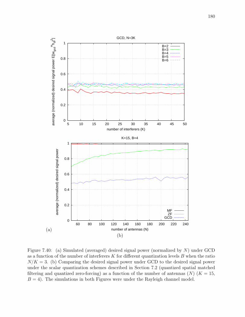
180

0

0.2

0.4

0.6

0.8

1

5 10 15 20 25 30 35 40 45 50aver

age

(nor

mal

ized

) de

sire

d si

gnal

pow

er E

[|wgc

dHh d

|2 ]

number of interferers (K)

GCD, N=3K

B=2B=3B=4B=5B=6

(a)

0

0.2

0.4

0.6

0.8

1

60 80 100 120 140 160 180 200 220 240

aver

age

(nor

mal

ized

) de

sire

d si

gnal

pow

er

number of antennas (N)

K=15, B=4

MFZF

GCD

(b)

Figure 7.40: (a) Simulated (averaged) desired signal power (normalized by N) under GCDas a function of the number of interferers K for different quantization levels B when the ratioN/K = 3. (b) Comparing the desired signal power under GCD to the desired signal powerunder the scalar quantization schemes described in Section 7.2 (quantized spatial matchedfiltering and quantized zero-forcing) as a function of the number of antennas (N) (K = 15,B = 4). The simulations in both Figures were under the Rayleigh channel model.

181

-30

-25

-20

-15

-10

-5

0

5

10

60 80 100 120 140 160 180 200 220 240

10lo

g(N

*(av

erag

e in

terf

erer

pow

er))

number of antennas (N)

GCD, K=15

B=2B=3B=4B=5B=6

(a)

-65

-60

-55

-50

-45

-40

-35

-30

-25

-20

10 20 30 40 50 60 70 80

10lo

g((a

vera

ge in

terf

erer

pow

er)/

K)

number of interferers (K)

GCD, N=150

B=2B=3B=4B=5B=6

(b)

Figure 7.41: (a) Simulated (averaged) power of a single interferer (multiplied by N in dBscale) under GCD as a function of the number of antennas N for different quantization levelsB (K = 15). (b) Simulated (averaged) power of a single interferer (divided by K in dB scale)under GCD as a function of the number of interferers K for different quantization levels B(N = 150). The simulations in both Figures were under the Rayleigh channel model.

182

-45

-40

-35

-30

-25

-20

-15

-10

-5

5 10 15 20 25 30 35 40 45 50

aver

age

inte

rfer

er p

ower

(dB

)

number of interferers (K)

GCD, N=3K

B=2B=3B=4B=5B=6

(a)

-55

-50

-45

-40

-35

-30

-25

2 2.5 3 3.5 4 4.5 5 5.5 6

aver

age

inte

rfer

er p

ower

(dB

)

number of quantization bits (B)

GCD, N=245, K=15

GCD6dB/bit

(b)

Figure 7.42: (a) Simulated (averaged) power of a single interferer (in dB scale) in underGCD as a function of the number of interferers K for different quantization levels B whenthe ratio N/K = 3. (b) Simulated (averaged) power of a single interferer (in dB scale)under GCD as a function of the number of quantization bits B (N = 245, K = 10). Thesimulations in both Figures were under the Rayleigh channel model.

183

However, the difference is a constant factor (compared with the factor of N in interferencereduction). Therefore, a factor of N in Equation 7.4 comes from the desired signal andthe rest (22BN/K2) comes from the interference rejection. This is validated by the resultsin Figures 7.41/7.42, which plots the average interferer power under GCD versus N , K,and B. Figure 7.41a shows that the average interferer power scales as 1/N when K isfixed, while Figure 7.41b shows that the average interferer power increases linearly withK when N is fixed. Therefore, the average interferer power scales with the ratio K/N(Figure 7.42a). Furthermore, the gap between the different curves corresponding to thedifferent quantization levels is approximately 6dB indicating an exponential dependence onthe number of quantization bits B. Therefore, the total interference power scales as K2

N2−2B

(recall that we have a total K interferers).

Iterative greedy coordinate descent (iGCD)

The GCD algorithm improves the overall SIR by an extra factor of N/K, and achieves thiswith a computational complexity that grows linearly with N (as opposed to exponentially inthe case of exhaustive search). However, GCD still searches through all valid reconstructionlevels for each coefficient, and thus the running time grows exponentially with 2B. In thisSection, we present a variant of the conventional greedy coordinate descent algorithm calledthe iterative greedy coordinate descent algorithm or iGCD that eliminates the exponentialdependence on B, while retaining the extra factor of N/K in SIR improvement. iGCDcomputes the bits of each antenna weight separately, instead of searching over all 22B possibleweights as in GCD. We start by running GCD on the most significant bit of each weight.After converging on a single bit solution, the next iteration runs a single bit GCD for the nextsignificant bit. In this iteration, the most significant is fixed at the optimal solution foundin the previous iteration, and the search is only performed over the values of the second bit.This process is repeated B times (for each bit, while it is being modified, all previous moresignificant bits are fixed). Therefore, the overall running time will be linear in B instead ofexponential as in GCD.

Figures 7.43/7.44, 7.45/7.46, and 7.47/7.48 show the same results as Figures 7.37/7.38,7.39/7.40 and 7.41/7.42 for iGCD. These plots show that the behavior of iGCD is almostidentical to that of GCD. In Figure 7.55a, we plot both GCD and iGCD on the same graph.This shows that we incur no penalty by optimizing the quantized beamforming vector onebit at a time instead of searching all reconstruction levels.

Least significant bit-greedy coordinate descent (LSB-GCD)

A straight forward algorithm that can be derived directly from the proof in Section7.3.1 is least significant bit-greedy coordinate descent or LSB-GCD. LSB-GCD, as the namesuggests, is a variant of the general coordinate descent algorithm that optimizes only the leastsignificant bit or bits. In other words, we start with the quantized least squares (ZF) solution,then we optimize the least significant bit using GCD. Figures 7.49/7.50, 7.51/7.52, and7.53/7.54 show the simulation results for LSB-GCD (similar to Figures 7.37/7.38, 7.39/7.40,and 7.41/ 7.42). The plots show that LSB-GCD exhibits similar behavior to that of GCDand iGCD. A direct comparison between the three algorithms in Figure 7.55a shows that

184

-20

-10

0

10

20

50 100 150 200

10lo

g(E

[SIR

]/N2 )

number of antennas (N)

iGCD, K=15

B=2B=3B=4B=5B=6

(a)

45

50

55

60

65

70

75

80

85

20 40 60 80 100 120 140

10lo

g(K

2 E[S

IR])

number of interferers (K)

iGCD, N=150

B=2B=3B=4B=5B=6

(b)

Figure 7.43: (a) Simulated (averaged) SIR (normalized by N2 in dB scale) under iGCD asa function of the number of antennas N for different quantization levels B (K = 15). (b)Simulated (averaged) SIR (multiplied by K2 in dB scale) under iGCD as a function of thenumber of interferers K for different quantization levels B (N = 150). The simulations inboth Figures were under the Rayleigh channel model.

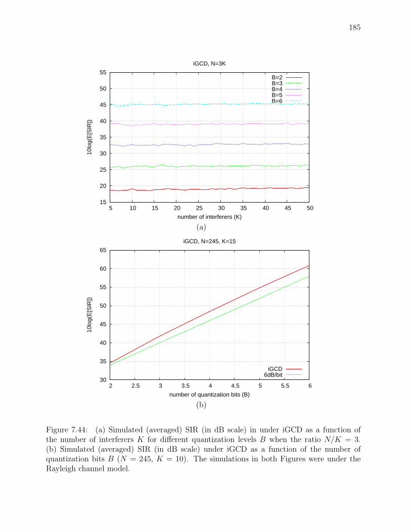
185

15

20

25

30

35

40

45

50

55

5 10 15 20 25 30 35 40 45 50

10lo

g(E

[SIR

])

number of interferers (K)

iGCD, N=3K

B=2B=3B=4B=5B=6

(a)

30

35

40

45

50

55

60

65

2 2.5 3 3.5 4 4.5 5 5.5 6

10lo

g(E

[SIR

])

number of quantization bits (B)

iGCD, N=245, K=15

iGCD6dB/bit

(b)

Figure 7.44: (a) Simulated (averaged) SIR (in dB scale) in under iGCD as a function ofthe number of interferers K for different quantization levels B when the ratio N/K = 3.(b) Simulated (averaged) SIR (in dB scale) under iGCD as a function of the number ofquantization bits B (N = 245, K = 10). The simulations in both Figures were under theRayleigh channel model.

186

0

0.2

0.4

0.6

0.8

1

50 100 150 200aver

age

(nor

mal

ized

) de

sire

d si

gnal

pow

er E

[|wig

cdH

h d|2 ]

number of antennas (N)

iGCD, K=15

B=2B=3B=4B=5B=6

(a)

0

0.2

0.4

0.6

0.8

1

20 40 60 80 100 120 140aver

age

(nor

mal

ized

) de

sire

d si

gnal

pow

er E

[|wig

cdH

h d|2 ]

number of interferers (K)

iGCD, N=150

B=2B=3B=4B=5B=6

(b)

Figure 7.45: (a) Simulated (averaged) desired signal power (normalized by N) under iGCDas a function of the number of antennas N for different quantization levels B (K = 15). (b)Simulated (averaged) desired signal power (normalized by N) under iGCD as a function ofthe number of interferers K for different quantization levels B (N = 150). The simulationsin both Figures were under the Rayleigh channel model.

187

0

0.2

0.4

0.6

0.8

1

5 10 15 20 25 30 35 40 45 50aver

age

(nor

mal

ized

) de

sire

d si

gnal

pow

er E

[|wig

cdH

h d|2 ]

number of interferers (K)

iGCD, N=3K

B=2B=3B=4B=5B=6

(a)

0

0.2

0.4

0.6

0.8

1

60 80 100 120 140 160 180 200 220 240

aver

age

(nor

mal

ized

) de

sire

d si

gnal

pow

er

number of antennas (N)

K=15, B=4

MFZF

iGCD

(b)

Figure 7.46: (a) Simulated (averaged) desired signal power (normalized by N) under iGCDas a function of the number of interferers K for different quantization levels B when the ratioN/K = 3. (b) Comparing the desired signal power under iGCD to the desired signal powerunder the scalar quantization schemes described in Section 7.2 (quantized spatial matchedfiltering and quantized zero-forcing) as a function of the number of antennas (N) (K = 15,B = 4). The simulations in both Figures were under the Rayleigh channel model.

188

-30

-25

-20

-15

-10

-5

0

5

10

60 80 100 120 140 160 180 200 220 240

10lo

g(N

*(av

erag

e in

terf

erer

pow

er))

number of antennas (N)

iGCD, K=15

B=2B=3B=4B=5B=6

(a)

-65

-60

-55

-50

-45

-40

-35

-30

-25

-20

10 20 30 40 50 60 70 80

10lo

g((a

vera

ge in

terf

erer

pow

er)/

K)

number of interferers (K)

iGCD, N=150

B=2B=3B=4B=5B=6

(b)

Figure 7.47: (a) Simulated (averaged) power of a single interferer (multiplied by N in dBscale) under iGCD as a function of the number of antennas N for different quantization levelsB (K = 15). (b) Simulated (averaged) power of a single interferer (divided by K in dB scale)under iGCD as a function of the number of interferers K for different quantization levels B(N = 150). The simulations in both Figures were under the Rayleigh channel model.

189

-50

-45

-40

-35

-30

-25

-20

-15

-10

-5

5 10 15 20 25 30 35 40 45 50

aver

age

inte

rfer

er p

ower

(dB

)

number of interferers (K)

iGCD, N=3K

B=2B=3B=4B=5B=6

(a)

-55

-50

-45

-40

-35

-30

-25

2 2.5 3 3.5 4 4.5 5 5.5 6

aver

age

inte

rfer

er p

ower

(dB

)

number of quantization bits (B)

iGCD, N=245, K=15

iGCD6dB/bit

(b)

Figure 7.48: (a) Simulated (averaged) power of a single interferer (in dB scale) in underiGCD as a function of the number of interferers K for different quantization levels B whenthe ratio N/K = 3. (b) Simulated (averaged) power of a single interferer (in dB scale)under iGCD as a function of the number of quantization bits B (N = 245, K = 10). Thesimulations in both Figures were under the Rayleigh channel model.

190

their performance is almost identical. While the desired signal power under LSB-GCD isslightly higher than both GCD and iGCD (Figure 7.55b), the interference power is alsoslightly higher (Figure 7.55c).

Impact of channel model

The proofs and simulation results presented in this section assumed a Rayleigh fadingmodel (i.e. the complex channel weights are i.i.d complex Gaussian random variables) forits simplicity. However, these results extend to other channel models as well. In Figure7.56, we compare the performance of iGCD under two extreme channel conditions: Rayleighfading and line of sight (LOS). For the LOS channel, we used both uniform linear and squarearrays with λ/2 spacing. For square arrays, we randomized the direction of arrival, whereasfor linear arrays, we only randomized the azimuth angle of arrival. In the figure, we plot theSIR (normalized by N2) on the y-axis versus the number of antennas N on the x-axis. Theresults show that the SIR maintains a quadratic growth as a function of N for both Rayleighand LOS channels.

Optimality of GCD based algorithms

Our simulations show that GCD-based algorithms converge after O(N) steps. However,a guaranteed convergence does not necessarily mean that it will converge to the optimumresult. In order to verify this, let us consider the impact of the initial state of the algorithmon the final output. If the algorithm is optimal, then it should converge to the same resultregardless of how the algorithm is initialized. In Sections 7.3.2 and 7.3.2, we did not tackle thequestion of initializing the GCD and iGCD algorithms, and assumed that both are initializedto the quantized matched filter. Here, we consider three different initializations: quantizedmatched filter, quantized ZF beamformer, and a random vector. Figure 7.57 shows theaverage SIR under iGCD for the three different initializations. To get a fair and accuratecomparison, we used the same values of hd,h1, . . . ,hK for each initialization. The plotsshow that even though the channel responses are the same, the average SIR changes whenwe change the initial state of the algorithm. These results suggest that these algorithmsconverge to local instead of global optima. However, this still does not tell us how far fromthe optimum is the GCD solution. To answer this question we simulated the average SIRusing a full exhaustive search of all possible quantized weight vectors. The results are shownin Figures 7.58ab. while it is difficult to draw conclusions from these graphs since we canonly simulate a full exhaustive search for small values of N and B, Figures 7.58ab suggestan exponential growth in average SIR as a function of N (K is fixed in Figure 7.58a) andan exponential decay as a function of K (N is fixed in Figure 7.58b). In [7], we derivedan upper bound on the achievable SIR and showed that it is indeed exponential, and theresults in Figure 7.58a would suggest that this bound is tight. Therefore, while GCD-basedalgorithms provide substantial improvements over scalar quantization, they are still far fromoptimum.

191

-20

-10

0

10

20

50 100 150 200

10lo

g(E

[SIR

]/N2 )

number of antennas (N)

LSB-GCD, K=15

B=2B=3B=4B=5B=6

(a)

45

50

55

60

65

70

75

80

20 40 60 80 100 120 140

10lo

g(K

2 E[S

IR])

number of interferers (K)

LSB-GCD, N=150

B=2B=3B=4B=5B=6

(b)

Figure 7.49: (a) Simulated (averaged) SIR (normalized by N2 in dB scale) under LSB-GCDas a function of the number of antennas N for different quantization levels B (K = 15). (b)Simulated (averaged) SIR (multiplied by K2 in dB scale) under LSB-GCD as a function ofthe number of interferers K for different quantization levels B (N = 150). The simulationsin both Figures were under the Rayleigh channel model.

192

15

20

25

30

35

40

45

50

55

5 10 15 20 25 30 35 40 45 50

10lo

g(E

[SIR

])

number of interferers (K)

LSB-GCD, N=3K

B=2B=3B=4B=5B=6

(a)

30

35

40

45

50

55

60

65

2 2.5 3 3.5 4 4.5 5 5.5 6

10lo

g(E

[SIR

])

number of quantization bits (B)

LSB-GCD, N=245, K=15

LSB-GCD6dB/bit

(b)

Figure 7.50: (a) Simulated (averaged) SIR (in dB scale) in under LSB-GCD as a functionof the number of interferers K for different quantization levels B when the ratio N/K = 3.(b) Simulated (averaged) SIR (in dB scale) under LSB-GCD as a function of the number ofquantization bits B (N = 245, K = 10). The simulations in both Figures were under theRayleigh channel model.

193

0

0.2

0.4

0.6

0.8

1

50 100 150 200

aver

age

(nor

mal

ized

) de

sire

d si

gnal

pow

er E

[|wls

b-gc

dHh d

|2 ]

number of antennas (N)

LSB-GCD, K=15

B=2B=3B=4B=5B=6

(a)

0

0.2

0.4

0.6

0.8

1

20 40 60 80 100 120 140

aver

age

(nor

mal

ized

) de

sire

d si

gnal

pow

er E

[|wls

b-gc

dHh d

|2 ]

number of interferers (K)

LSB-GCD, N=150

B=2B=3B=4B=5B=6

(b)

Figure 7.51: (a) Simulated (averaged) desired signal power (normalized by N) under LSB-GCD as a function of the number of antennas N for different quantization levels B (K = 15).(b) Simulated (averaged) desired signal power (normalized by N) under LSB-GCD as afunction of the number of interferers K for different quantization levels B (N = 150). Bothsimulations were under the Rayleigh channel model.

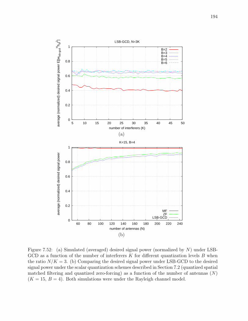
194

0

0.2

0.4

0.6

0.8

1

5 10 15 20 25 30 35 40 45 50

aver

age

(nor

mal

ized

) de

sire

d si

gnal

pow

er E

[|wls

b-gc

dHh d

|2 ]

number of interferers (K)

LSB-GCD, N=3K

B=2B=3B=4B=5B=6

(a)

0

0.2

0.4

0.6

0.8

1

60 80 100 120 140 160 180 200 220 240

aver

age

(nor

mal

ized

) de

sire

d si

gnal

pow

er

number of antennas (N)

K=15, B=4

MFZF

LSB-GCD

(b)

Figure 7.52: (a) Simulated (averaged) desired signal power (normalized by N) under LSB-GCD as a function of the number of interferers K for different quantization levels B whenthe ratio N/K = 3. (b) Comparing the desired signal power under LSB-GCD to the desiredsignal power under the scalar quantization schemes described in Section 7.2 (quantized spatialmatched filtering and quantized zero-forcing) as a function of the number of antennas (N)(K = 15, B = 4). Both simulations were under the Rayleigh channel model.

195

-30

-25

-20

-15

-10

-5

0

5

10

60 80 100 120 140 160 180 200 220 240

10lo

g(N

*(av

erag

e in

terf

erer

pow

er))

number of antennas (N)

LSB-GCD, K=15

B=2B=3B=4B=5B=6

(a)

-60

-55

-50

-45

-40

-35

-30

-25

-20

20 40 60 80 100 120 140

10lo

g((a

vera

ge in

terf

erer

pow

er)/

K)

number of interferers (K)

LSB-GCD, N=150

B=2B=3B=4B=5B=6

(b)

Figure 7.53: (a) Simulated (averaged) power of a single interferer (multiplied by N in dBscale) under LSB-GCD as a function of the number of antennas N for different quantizationlevels B (K = 15). (b) Simulated (averaged) power of a single interferer (divided by K in dBscale) under LSB-GCD as a function of the number of interferers K for different quantizationlevels B (N = 150). Both simulations were under the Rayleigh channel model.

196

-45

-40

-35

-30

-25

-20

-15

-10

-5

5 10 15 20 25 30 35 40 45 50

aver

age

inte

rfer

er p

ower

(dB

)

number of interferers (K)

LSB-GCD, N=3K

B=2B=3B=4B=5B=6

(a)

-50

-45

-40

-35

-30

-25

-20

2 2.5 3 3.5 4 4.5 5 5.5 6

aver

age

inte

rfer

er p

ower

(dB

)

number of quantization bits (B)

LSB-GCD, N=245, K=15

LSB-GCD6dB/bit

(b)

Figure 7.54: (a) Simulated (averaged) power of a single interferer (in dB scale) in underLSB-GCD as a function of the number of interferers K for different quantization levels Bwhen the ratio N/K = 3. (b) Simulated (averaged) power of a single interferer (in dB scale)under LSB-GCD as a function of the number of quantization bits B (N = 245, K = 10).Both simulations were under the Rayleigh channel model.

197

(a)

-10

-5

0

5

10

60 80 100 120 140 160 180 200 220 240

10lo

g(E

[SIR

]/N2 )

number of antennas (N)

K=15, B=4

GCDiGCD

LSB-GCD

(b)

0

0.2

0.4

0.6

0.8

1

60 80 100 120 140 160 180 200 220 240

aver

age

desi

red

sign

al p

ower

number of antennas (N)

K=15, B=4

GCDiGCD

LSB-GCD

(c)

-42

-40

-38

-36

-34

-32

-30

-28

60 80 100 120 140 160 180 200 220 240

aver

age

inte

rfer

er p

ower

(dB

)

number of antennas (N)

K=15, B=4

GCDiGCD

LSB-GCD

Figure 7.55: Comparing the performance of three vector quantization techniques (GCD,iGCD, LSB-GCD) versus the number of antennas (N) under a Rayleigh channel model(K = 15 and B = 4). (a) Average SIR normalized by N2 in dB scale. (b) Desired signalpower (normalized by N). (c) Average interferer power in dB scale.

198

-40

-30

-20

-10

0

10

50 100 150 200

10lo

g(E

[SIR

]/N2 )

number of antennas (N)

iGCD, K=15, B=3

square arraylinear array

Rayleigh

Figure 7.56: Performance of iGCD under different channel models (Rayleigh/LOS). On thex-axis, the number of antennas (N). On the y-axis, the average SIR (normalized by N2) indB scale. The number of interferers and bits are fixed at K = 15 and B = 3 respectively.

199

-6

-4

-2

0

2

4

6

60 80 100 120 140 160 180 200 220 240

10lo

g(E

[SIR

]/N2 )

number of antennas (N)

K=15, B=4

iGCD-MFiGCD-ZF

iGCD-random

Figure 7.57: Average SIR normalized by N2 under iGCD, for three different initializations(quantized matched filter, quantized zero-forcer, and random quantized vector), versus thenumber of antennas N (the x-axis), with a fixed number of interferers K = 15, and quanti-zation bits B = 4. The simulation was under the Rayleigh channel model.

200

10

15

20

25

30

35

40

5 6 7 8 9 10

SIR

(dB

)

number of antennas (N)

1-bit exhaustive search/LOS

(a)

10

20

30

40

50

60

70

80

90

1 2 3 4 5 6

SIR

(dB

)

number of interferers (K)

1-bit exhaustive search/LOS

(b)

Figure 7.58: (a) Average SIR under exhaustive (optimal) searching versus the numberof antennas N (the x-axis), with a fixed number of interferers K = 2, and quantizationbits B = 1. (b) Average SIR under exhaustive (optimal) searching versus the number ofinterferers K (the x-axis), with a fixed number of antennas N = 10, and quantization bitsB = 1. The simulation was under an LOS channel model with a uniform linear array withλ/2 spacing.

201

Computation complexity

Simulation results show that the number of steps (iterations) required for convergence isproportional N (for all three algorithms). At each step, the SIR needs to be re-evaluated.However, since we are only changing one coefficient at a time, the number of complex oper-ations (multiplications/additions) needed to compute (update) the new SIR is proportionalto K. Since both GCD and iGCD can be initialized using the scalar quantized matchedfilter (requires only O(N) operations), the total number operations required to computethe GCD and iGCD solutions is O(NK22B) and O(NKB) respectively9. Since LSB-GCDonly works with the least significant bit(s), it eliminates the dependence on B. However,LSB-GCD requires computing the least-squares (ZF) solution as a starting point. This re-quires O(NK2) operations. Therefore, the total running time of LSB-GCD is proportionalto O(NK2). Therefore, if K ≫ B, then the iGCD can even outperform the scalar quantizedZF beamformer from a computational complexity standpoint.

Switched antenna arrays

In Chapter 2, we listed several alternative architectures for implementing dynamic beam-forming in addition to phased antenna arrays, including switched antenna arrays and switchedparasitic antennas. While the underlying theory and physical properties behind these dif-ferent architectures may differ, they all share several key properties. First, they all requirean array of antennas10. Second, the overall gain (if well designed) is proportional to the sizeof the array. Finally, in all the architectures, some aspect (weight) of each antenna elementis dynamically controlled. Therefore, from a mathematical point view, all these differentantenna systems can be represented by a size N complex column vector of beamformingweights (channel responses). The universe from which these weights can be drawn will bedifferent for each architecture. For switched antenna arrays and switched parasitic anten-nas, this universe is usually 0, 1N (i.e. antennas are either turn on or off). This very lowresolution makes vector quantization algorithms like GCD a natural fit for these systems.

The performance is similar to GCD with conventional I/Q quantization. The SIR growsalmost quadratically with the ratio N/K (Figure 7.59a shows quadratic increase with Nwhile Figure 7.59b shows a fixed SIR when N/K is fixed). The desired signal grows linearlywith N and is largely independent of the number of interferers K (Figures 7.61ab), whilethe average interferer power shrinks with N/K (Figures 7.60ab).

7.3.3 Improving the beamforming gain using vector quantization

Our focus in this chapter has been almost exclusively on improving the interferencesuppression since the beam nulls tend to be a lot more sensitive to weight errors than peaks.However, even in the absence of interference, the signal to noise ratio (SNR) can still beimproved by using a vector quantization technique like GCD or iGCD although the extragain from using these techniques will be very small since the loss from scalar quantization is

9GCD is exponentially dependent on B while iGCD is only linearly dependent on B.10Not all these antennas are necessarily driven by a signal, and may act only as passive reflectors (e.g.

switched parasitics).

202

-32

-31

-30

-29

-28

-27

-26

-25

50 100 150 200 250 300 350 400 450 500

10lo

g(E

[SIR

]/N2 )

number of antennas (N)

Rayleigh channel, K=15

GCD/random initializationGCD/MF initialization

(a)

-4

-2

0

2

4

6

8

10

10 20 30 40 50 60 70 80 90 100

10lo

g(E

[SIR

])

number of interferers (K)

Rayleigh channel, N=3K

GCD/random initializationGCD/MF initialization

(b)

Figure 7.59: (a) Average SIR normalized by N2 under GCD with two quantization levels0, 1 versus the number of antennas N (the x-axis), with a fixed number of interferersK = 15. (b) Average SIR under GCD with two quantization levels 0, 1 versus the numberof interferers K (the x-axis), when the ratio N/K is fixed. The plots in this figure used theRayleigh channel model.

203

12

14

16

18

20

22

24

50 100 150 200 250 300 350 400 450 500

N*(

inte

rere

nce

pow

er)

(dB

)

number of antennas (N)

Rayleigh channel, K=15

GCD/random initializationGCD/MF initialization

(a)

-20

-15

-10

-5

0

10 20 30 40 50 60 70 80 90 100

(inte

rere

nce

pow

er)

(dB

)

number of interferers (K)

Rayleigh channel, N=3K

GCD/random initializationGCD/MF initialization

(b)

Figure 7.60: (a) Average interferer power multiplied by N (in dB scale) under GCD withtwo quantization levels 0, 1 versus the number of antennas N (the x-axis), with a fixednumber of interferers K = 15. (b) Average interferer power (in dB scale) under GCD withtwo quantization levels 0, 1 versus the number of interferers K (the x-axis), when the ratioN/K is fixed. The plots in this figure used the Rayleigh channel model.

204

0

0.2

0.4

0.6

0.8

1

50 100 150 200 250 300 350 400 450 500

norm

aliz

ed b

eam

form

ing

gain

number of antennas (N)

Rayleigh channel, K=15

GCD/random initializationGCD/MF initialization

(a)

0

0.2

0.4

0.6

0.8

1

10 20 30 40 50 60 70 80 90 100

norm

aliz

ed b

eam

form

ing

gain

number of interferers (K)

Rayleigh channel, N=3K

GCD/random initializationGCD/MF initialization

(b)

Figure 7.61: (a) Normalized desired signal gain under GCD with two quantization levels0, 1 versus the number of antennas N (the x-axis), with a fixed number of interferersK = 15. (b) Normalized desired signal gain under GCD with two quantization levels 0, 1versus the number of interferers K (the x-axis), when the ratio N/K is fixed. The plots inthis figure used the Rayleigh channel model.

205

already small to begin with as we showed in Chapter6. Figure 7.62a shows the normalizedbeamforming gain of the scalar quantized matched filter and the GCD quantizer for twoquantization levels: B = 1 and B = 1/2 (for a Rayleigh channel) 11. The graph shows thatGCD provides a slight improvement over a scalar quantizer and the gap gets smaller as weincrease N and B. Furthermore, GCD is still below the optimum though the gap is extremelysmall (Figure 7.63a shows that the normalized beamforming gain is slightly below optimumsolution obtained by exhaustive search). Figure 7.64a shows the normalized beamforminggain when GCD is initialized to two different values (the quantized matched filter and arandom vector). The graph shows that the final result is slightly different depending onhow we initialize the GCD algorithm, which shows that GCD does not converge to a globalminimum. However, the difference is almost negligible. Figures 7.62b, 7.63b, and 7.64b showthat the same results hold for an LOS channel (a uniform linear array (λ/2 spaced) with theazimuth angle chosen randomly and the elevation angle fixed at 90 from the z-axis) as well.

7.4 Conclusion

In this chapter, we have shown that coefficient quantization in digital receiver implemen-tations can have a profound effect on the performance of interference-limited multi-antennasystems. In particular, quantization of beamforming weights critically affects interferencesuppression performance, and must be performed carefully in order to exploit the degreesof freedom gains from using an increased number of antennas. We have analyzed the per-formance of both scalar and vector quantization techniques, and presented computationallyefficient greedy sequential quantization algorithms that provide substantial gains over naivescalar quantization. However, we have also shown that the interference rejection achieved bythose algorithms (polynomial in the number of antennas) is still far from optimum (exponen-tial in the number of antennas). Important open problems include refinement of the analysisto provide tight upper and lower bounds on SIR scaling, and devising efficient algorithmsfor finding the quantized weights that approach the performance of the optimal quantizedweights.

11B = 1 corresponds to four quantization levels: 1 + j, 1 − j,−1 + j,−1 − j. B = 1/2 corresponds totwo quantization levels: 1,−1

206

0

0.2

0.4

0.6

0.8

1

50 100 150 200 250 300 350 400 450 500

norm

aliz

ed s

igna

l gai

n

number of antennas (N)

scalar (B=1/2)GCD (B=1/2)scalar (B=1)GCD (B=1)

(a)

0

0.2

0.4

0.6

0.8

1

50 100 150 200 250 300 350 400 450 500

norm

aliz

ed s

igna

l gai

n

number of antennas (N)

scalar (B=1/2)GCD (B=1/2)scalar (B=1)GCD (B=1)

(b)

Figure 7.62: Normalized beamforming gain under GCD and scalar quantization (quantizedmatched filtering) versus the number of antennas N for two different quantization levels(B = 1, 1

2): (a) Rayleigh channel. (b) LOS channel (a uniform linear array with a λ/2

spacing).

207

0

0.2

0.4

0.6

0.8

1

2 3 4 5 6 7 8 9 10

norm

aliz

ed b

eam

form

ing

gain

number of antennas (N)

Rayleigh channel

GCD (B=1/2)Exhaustive Search (B=1/2)

GCD (B=1)Exaustive Search (B=1)

(a)

0

0.2

0.4

0.6

0.8

1

2 3 4 5 6 7 8 9 10

norm

aliz

ed b

eam

form

ing

gain

number of antennas (N)

LOS channel (linear array)

GCD (B=1/2)Exhaustive Search (B=1/2)

GCD (B=1)Exaustive Search (B=1)

(b)

Figure 7.63: Normalized beamforming gain under GCD and exhaustive search versus thenumber of antennas N for two different quantization levels (B = 1, 1

2): (a) Rayleigh channel.

(b) LOS channel (a uniform linear array with a λ/2 spacing).

208

0.33

0.332

0.334

0.336

0.338

0.34

0.342

0.344

0.346

0.348

0.35

50 100 150 200 250 300 350 400 450 500

norm

aliz

ed b

eam

form

ing

gain

number of antennas (N)

GCD, Rayleigh channel

B=1/2 (matched filter)B=1/2 (random)

(a)

0.44

0.445

0.45

0.455

0.46

0.465

0.47

0.475

0.48

50 100 150 200 250 300 350 400 450 500

norm

aliz

ed b

eam

form

ing

gain

number of antennas (N)

GCD, LOS channel (uniform linear array)

B=1/2 (matched filter)B=1/2 (random)

(b)

Figure 7.64: Normalized beamforming gain under GCD with two different initializations(quantized matched filter and a random initialization) versus the number of antennas Nfor two different quantization levels (B = 1, 1

2): (a) Rayleigh channel. (b) LOS channel (a

uniform linear array with a λ/2 spacing).

209

Chapter 8

Conclusion and future work

In this work, we have presented an architecture for building high gain adaptive an-tenna array systems for long range and high capacity systems. The hardware componentof the proposed architecture covers both the radio circuit design as well as the antennadesign. We found that a hybrid RF/digital beamforming radio architecture provides thebest trade off between performance (speed/precision/bandwidth) on the one hand, and cost(complexity/power consumption) on the other hand. We also found that we can utilize 3-dimensional array structures to improve the signal to noise ratio and the beam scan angle.These structures are more compact than traditional planar antennas. In both cases, weproposed different techniques for implementing the radio and antenna architecture with lowcost technologies like integrated circuits and printed circuit boards.

The software component of the framework is composed of signal processing and adap-tive algorithms for optimizing the performance of arrays that utilize our proposed hardwarearchitecture. We introduced signal processing techniques that improve the performance ofconventional adaptive filters used for beamforming in the presence of adverse channel condi-tions (e.g. noise, interference, fast fading and frequency offsets). We also proposed compu-tationally efficient vector quantization techniques for improving the interference suppressionunder low resolution and error prone RF and analog beamformers in large arrays.

Up to this point, we have validated our approach mostly with mathematical proofs andcomputer simulations. The next logical step would be to implement those techniques inhardware and test them in real world settings. Some of this work is already underway. Wehave already built several prototypes of phased array antennas with 16 and 32 elementsoperating at frequency bands in the 2.4GHz and 5GHz range (WiFi bands). The prototypeswere built with discrete circuit components mounted on PCBs. So far we have had successwith initial lab tests and some limited outdoor tests. However, more rigorous testing isrequired before these prototypes can be deployed in a large scale outdoor testbed.

The next major step in fulfilling our ultimate goal is the realization of a fully integratedbeamforming solution. Although our project has been mainly focused on frequencies nearcellular bands (e.g. ISM bands), There are ongoing parallel efforts at the Berkeley WirelessResearch Center for building and testing a fully integrated phased array system at 60GHz[4, 52, 34, 56]. As of now (December 2010), The project is at the stage where a fully integrated4-channel phased array transceiver has been built and successfully tested (in 65nm CMOSprocess) [56].

210

There also remains a lot of work to be done on the algorithms side. We showed that eventhough our proposed vector quantization algorithms improve the performance of the arrayby a factor proportional to the number of antennas compared with scalar techniques, thereis still a lot of room for improvement. The performance of the techniques we have proposedis quadratic in the number of antennas, whereas an exhaustive search of all reconstructionlevels can be exponential. Therefore, designing a tractable algorithm that approaches thisupper bound remains an open problem.

Another direction we would like to pursue in the future is to consider the impact ofincorporating beamforming and adaptive antenna techniques on the design of higher layersin the network stack. In this work, we have restricted our attention to the physical layer.However, existing higher layers in the protocol stack (e.g. MAC, network, transport) havenot taken into account recent advances in wireless technologies when originally designed.In fact, some of these protocols, like TCP, have not been designed with wireless networksin mind. Therefore, care must by taken when introducing new technologies to ensure thatthe performance of upper layer protocols is not adversely affected. At the same time, weneed to consider how to design future networking protocols in order to take full advantage ofstate of the art technologies in the wireless space, and how much improvement in the systemperformance can be achieved when the different components of the system are designedjointly compared when they are designed independently. There has already been some workin this area [51, 16, 17, 19, 18]. However, we believe we barely scratched the surface.

211

Bibliography

[1] www.ansoft.com.

[2] Cisco Visual Networking Index: Global Mobile Data Traffic Forecast Update, 2009-2014. http://www.cisco.com/en/US/solutions/collateral/ns341/ns525/ns537/ns705/ns827/white paper c11-520862.html.

[3] E. Adabi and A. Niknejad. Broadband variable passive delay elements based on aninductance multiplication technique. In Proc. of IEEE Radio Frequency Integrated Cir-cuits Symposium (RFIC), June 2008.

[4] S. Alalusi. A 60GHz Adaptive Antenna Array in CMOS. PhD thesis, University ofCalifornia at Berkeley, Berkeley, CA, USA, 2005.

[5] S. Alalusi and R. Broderson. A 60GHz Phased Array in CMOS. In Proc. of IEEECustom Integrated Circuits Conference, September 2006.

[6] O. Bakr and M. Johnson. Impact of phase and amplitude errors on array perfor-mance. Technical Report UCB/EECS-2009-1, EECS Department, University of Cal-ifornia, Berkeley, January 2009.

[7] O. Bakr, M. Johnson, R. Mudumbai, and U. Madhow. Interference suppression in thepresence of quantization errors. In Allerton Conference on Communication, Control,and Computing, September 2009.

[8] O. Bakr, M. Johnson, R. Mudumbai, and K. Ramchandran. Multi-antenna InterferenceCancellation Techniques for Cognitive Radio Applications. In Proc. of IEEE WirelessComunications and Networking Conference, April 2009.

[9] O. Bakr, M. Johnson, J. Park, E. Adabi, K. Jones, and A. Niknejad. A Scalable, LowCost Architecture for High Gain Beamforming Antennas. In Proc. of IEEE InternationalSymposium on Phased Array Systems and Technology, October 2010.

[10] O. Bakr, M. Johnson, B. Wild, and K. Ramchandran. A multi-antenna framework forspectrum reuse based on primary-secondary cooperation. In IEEE Symposium on NewFrontiers in Dynamic Spectrum Access Networks (DySPAN), October 2008.

[11] O. Bakr, M. Johnson, B. Wild, and K. Ramchandran. Performance analysis of a multi-antenna framework for spectrum reuse. Technical Report UCB/EECS-2008-101, EECSDepartment, University of California, Berkeley, August 2008.

212

[12] C. Balanis. Antenna Theory. John Wiley & Sons, 2005.

[13] F. Behbahani, Y. Kishigami, J. Leete, and A.A. Abidi. CMOS mixers and polyphasefilters for large image rejection. IEEE Journal of Solid-State Circuits, 36(6):873–887,June 2001.

[14] J. Blass. Multidirectional Antenna: A New Approach to Stacked Beams. IRE Interna-tional Conference Record, 8(1), 1960.

[15] J. Butler and R. Lowe. Beam-Forming Matrix Simplifies Design of ElectronicallyScanned Antennas. Electronic Design, pages 170–173, 1961.

[16] R. R. Choudhury and Nitin Vaida. Performance of Ad Hoc Routing using DirectionalAntennas. Elsevier Ad Hoc Networks Journal, November 2004.

[17] R. R. Choudhury and Nitin Vaida. On Designing MAC Protocols for Wireless Networksusing Beamforming Antennas. IEEE Transactions of Mobile Computing (TMC), May2006.

[18] R. R. Choudhury and N. Vaidya. Deafness: A MAC Problem in Ad Hoc Networks whenusing Directional Antennas. In IEEE ICNP, September 2004.

[19] R. R. Choudhury, X. Yang, R. Ramanathan, and N. Vaidya. Using Directional Antennasfor Medium Access Control in Ad Hoc Networks. In ACM MOBICOM, September 2002.

[20] D. Chowdhury, C. Hull, O. Degani, Y. Wang, and A. Niknejad. A Fully Integrated Dual-Mode Highly Linear 2.4 GHz CMOS Power Amplifier for 4G WiMax Applications. IEEEJournal of Solid-State Circuits, 44(12):3393–2402, December 2009.

[21] C. B. Dietrich. Adaptive Arrays and Diversity Antenna Configurations for HandheldWireless Communication Terminals. PhD thesis, Virginia Polytechnic Institute, Blacks-burg, VA, USA, 2000.

[22] H. Dogan, R. Meyer, and A. Niknejad. A DC-10GHz Linear-in-dB Attenuator in 0.13µmCMOS Technology. In Proc. of IEEE Custom Integrated Circuits Conference, November2004.

[23] D. Ehyaie and A. Mortazawi. A 24 GHz Modular Phased Array Based on ExtendedResonance Technique. In Proc. of IEEE International Symposium on Phased ArraySystems and Technology, October 2010.

[24] P. Haldi, D. Chowdhury, P. Reynaert, G. Liu, and A. Niknejad. A 5.8 GHz 1 V LinearPower Amplifier Using a Novel On-Chip Transmormer Power Combiner in Standard 90nm CMOS. IEEE Journal of Solid-State Circuits, 45(5):1054–1063, May 2008.

[25] H. Hashemi, X. Guan, A. Komijani, and A. Hajimiri. A 24-ghz sige phased-arrayreceiver-lo phase-shifting approach. IEEE Transactions on Microwave Theory and Tech-niques, 53(2):614–26, February 2005.

213

[26] M. Hayes. Statistical Digital Signal Processing and Modeling. Wiley, 1996.

[27] S. Haykin. Adaptive Filter Theory. Prentice Hall, 2002.

[28] T. Lee. The Desigh of CMOS Radio-Frequency Integrated Circuits. Cambridge Univer-sity Press, 2004.

[29] J. C. Liberti and T. Rappaport. Smart Antennas for Wireless Communications: IS-95and Third Generation CDMA Applications. Prentice Hall, 1999.

[30] X. Liu, A. Sheth, M. Kaminsky, K. Papagiannaki, S. Seshan, and P. Steenkiste. DIRC:increasing indoor wireless capacity using directional antennas. In ACM SIGCOMM,2009.

[31] U. Madhow, K. Bruvold, and L. J. Zhu. Differential MMSE: A framework for robustadaptive interference suppression for DS-CDMA over fading channels. IEEE Transac-tions on Communications, 53(8):1377–1390, Aug. 2005.

[32] A. Mainwaring, A. L. Umnov, V. A. Filimonov, I. S. Shishalov, and M. Shuralev. Theo-retical and Experimental Investigations of Adaptive Reactance Parasitic Antenna Array.In Mobile and Wireless Communications Summit, 2007.

[33] D. Manolakis, V. Ingle, and S. Kogon. Statistical and Adaptive Signal Processing: Spec-tral Estimation, Signal Modeling, Adaptive Filtering and Array Processing. McGraw-Hill, 2000.

[34] C. Marcu, D. Chowdhury, C. Thakkar, J. Park, L. Kong, M. Tabesh, Y. Wang, B. Af-shar, A. Gupta, A. Arbabian, S. Gambini, R. M. Zamani, E. Alon, and A. Niknejad.A 90nm cmos low-power 60 ghz transceiver with integrated baseband circuitry. IEEEJournal of Solid-State Circuits, 44(12), December 2009.

[35] S. M. Mishra, J. Hwang, D. Filippini, T. Du, R. Moazzami, and L. Subramanian.Economic Analysis of Networking Technologies for Rural Developing Regions. In WINE,December 2005.

[36] R. Mudumbai, J. Hespanha, and U. Madhow. Scalable feedback control for distributedbeamforming in sensor networks. In IEEE International Symposium on InformationTheory (ISIT), September 2005.

[37] R. Mudumbai, B. Wild, U. Madhow, and K. Ramchandran. Distributed beamformingusing 1 bit feedback: from concept to realization. In Allerton Conference on Commu-nication, Control, and Computing, September 2006.

[38] A. Natarajan, A. Komijani, and A. Hajimiri. A Fully Integrated 24-GHz Phased-ArrayTransmitter in CMOS. IEEE Journal of Solid-State Circuits, 40(12):2502–14, December2005.

[39] S. Nedevschi, R. Patra, S. Surana, S. Ratnasamy, L. Subramanian, and E. Brewer. AnAdaptive, High Performance MAC for Long-Distance Multihop Wireless Networks. InACM MOBICOM, 2008.

214

[40] A. Niknejad, M. Bohsali, E. Adabi, and B. Heydari. Integrated circuit transmission-line transformer power combiner for millimetre-wave applications. Electronic Letters,43(5):290–291, March 2007.

[41] A. Niknejad and H. Hashemi. mm-Wave Silicon Technology: 60 GHz and Beyond.Springer, 2008.

[42] A. Oppenheim and R. Schafer. Discrete-Time Signal Processing. Prentice Hall, 1999.

[43] J. Paramesh, R. Bishop, K. Soumyanath, and D.J. Allstot. A 1.4V 5GHz four-antennaCartesian-combining receiver in 90nm CMOS for beamforming and spatial diversityapplications. In Proc. of IEEE International Solid-State Circuits Conference, February2005.

[44] R. Patra. A Multi-Tier Network Architecture for Long Distance Rural WirelessNetworksin Developing Regions. PhD thesis, University of California at Berkeley, Berkeley, CA,USA, 2009.

[45] D. Pozar. Microwave Engineering. John Wiley & Sons, 2005.

[46] J. G. Proakis and D. G. Manolakis. Digital Signal Processing: Principles, Algorithms,and Applications. Prentice Hall, 1996.

[47] J. G. Proakis and M. Salehi. Communication Systems Engineering. Prentice Hall, 2002.

[48] RNCOS. Emerging Mobile Wireless Technologies – Road to a Wireless World, 2005.

[49] K. Rosen. Discrete Mathematics and its Applications. McGraw Hill, 2007.

[50] A. Sayed. Adaptive Filter. Wiley & Sons, 2008.

[51] S. Sen, X. Jie, R. Ghosh, and R. R. Choudhury. Link Layer Multicast using SmartAntennas: No Client Left Behind. In IEEE ICNP, 2008.

[52] D. Sobel. A Baseband Mixed-Signal Receiver Front-End for 1Gbps Wireless Communi-cations at 60GHz. PhD thesis, University of California at Berkeley, Berkeley, CA, USA,2008.

[53] G. Strang. Linear Algebra and Its Applications. Thomson Learning, 1988.

[54] W. Stutzman and G. Thiele. Antenna Theory and Design. John Wiley & Sons, 1998.

[55] S. Surana, R. Patra, S. Nedevschi, M. Ramos, L. Subramanian, Y. Ben-David, andE. Brewer. Beyond Pilots: Keeping Rural Wireless Networks Alive. In NSDI, 2008.

[56] M. Tabesh, J. Chen, C. Marcu, L. Kong, S. Kang, E. Alon, and A. Niknejad. A 65nmCMOS 4-Element Sub-34mW/Element 60GHz Phased-Array Transceiver. In Proc. ofIEEE International Solid-State Circuits Conference, To appear in February 2011.

[57] D. V. Thiel and S. Smith. Switched Paracitic Antennas for Cellular Communications.Artech House, 2002.

215

[58] H.L. Van Trees. Optimum Array Processing. Wiley-Interscience, 2002.

[59] D. Tse and P. Viswanath. Fundamentals of Wireless Communications. CambridgeUniversity Press, 2005.

[60] F. Ulaby. Fundamentals of Applied Electromagnetics. Prentice Hall, 2004.

[61] H. Wang and A. Hajimiri. A Wideband CMOS Linear Digital Phase Rotator. In Proc.of IEEE Custom Integrated Circuits Conference, September 2007.

[62] M. R. Williamson, G. E. Athanasiadou, and A. R. Nix. Investigating the effects ofantenna directivity on wireless indoor communication at 60GHz. In Proceedings of thePIMRC Conference, 1997.

[63] H. Zarei, C.T. Charles, and D.J. Allstot. Reflective-type phase shifters for multiple-antenna transceivers. IEEE Transactions on Circuits and Systems I: Fundamental The-ory and Applications, 54(8):1647–56, August 2007.